Download EViews 4.0 User's Guide

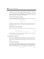
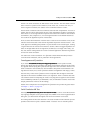
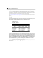
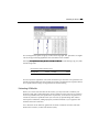
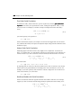
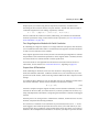
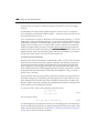
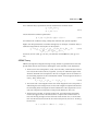
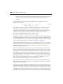
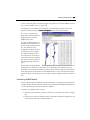
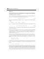
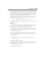
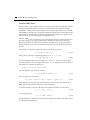
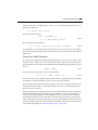
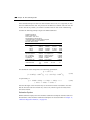
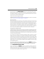
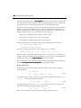
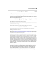
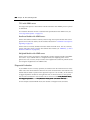
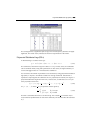
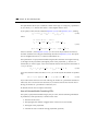
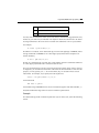
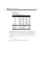
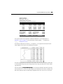
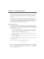
Chapter 13. Time Series Regression
In this section we discuss single equation regression techniques that are important for the
analysis of time series data: testing for serial correlation, estimation of ARMA models,
using polynomial distributed lags, and testing for unit roots in potentially nonstationary
time series.
The chapter focuses on the specification and estimation of time series models. A number
of related topics are discussed elsewhere: standard multiple regression techniques are discussed in Chapters 11 and 12, forecasting and inference are discussed extensively in
Chapters 14 and 15, vector autoregressions are discussed in Chapter 20, and state space
models and the Kalman filter are discussed in Chapter 22.
Serial Correlation Theory
A common finding in time series regressions is that the residuals are correlated with their
own lagged values. This serial correlation violates the standard assumption of regression
theory that disturbances are not correlated with other disturbances. The primary problems
associated with serial correlation are:
• OLS is no longer efficient among linear estimators. Furthermore, since prior residuals help to predict current residuals, we can take advantage of this information to
form a better prediction of the dependent variable.
• Standard errors computed using the textbook OLS formula are not correct, and are
generally understated.
• If there are lagged dependent variables on the right-hand side, OLS estimates are
biased and inconsistent.
EViews provides tools for detecting serial correlation and estimation methods that take
account of its presence.
In general, we will be concerned with specifications of the form:
y t = x t ′¯ + u t
u t = z t − 1 ′° + " t
(13.1)
where x t is a vector of explanatory variables observed at time t, z t − 1 is a vector of variables known in the previous period, b and g are vectors of parameters, u t is a disturbance
term, and " t is the innovation in the disturbance. The vector z t − 1 may contain lagged
values of u, lagged values of e, or both.
296—Chapter
13. Time Series Regression
296
The disturbance u t is termed the unconditional residual. It is the residual based on the
′
structural component ( x t ¯ ) but not using the information contained in z t − 1 . The innovation " t is also known as the one-period ahead forecast error or the prediction error. It is the
difference between the actual value of the dependent variable and a forecast made on the
basis of the independent variables and the past forecast errors.
The First-Order Autoregressive Model
The simplest and most widely used model of serial correlation is the first-order autoregressive, or AR(1), model. The AR(1) model is specified as
y t = x t ′¯ + u t
u t = ½u t − 1 + " t
(13.2)
The parameter r is the first-order serial correlation coefficient. In effect, the AR(1) model
incorporates the residual from the past observation into the regression model for the current observation.
Higher-Order Autoregressive Models
More generally, a regression with an autoregressive process of order p, AR(p) error is given
by
y t = x t ′¯ + u t
u t = ½ 1u t − 1 + ½2 u t − 2 + … + ½ p u t − p + " t
(13.3)
The autocorrelations of a stationary AR(p) process gradually die out to zero, while the partial autocorrelations for lags larger than p are zero.
Testing for Serial Correlation
Before you use an estimated equation for statistical inference (e.g. hypothesis tests and
forecasting), you should generally examine the residuals for evidence of serial correlation.
EViews provides several methods of testing a specification for the presence of serial correlation.
The Durbin-Watson Statistic
EViews reports the Durbin-Watson (DW) statistic as a part of the standard regression output. The Durbin-Watson statistic is a test for first-order serial correlation. More formally,
the DW statistic measures the linear association between adjacent residuals from a regression model. The Durbin-Watson is a test of the hypothesis r = 0 in the specification:
u t = ½u t − 1 + " t .
(13.4)
Testing for Serial Correlation—297
297
If there is no serial correlation, the DW statistic will be around 2. The DW statistic will fall
below 2 if there is positive serial correlation (in the worst case, it will be near zero). If
there is negative correlation, the statistic will lie somewhere between 2 and 4.
Positive serial correlation is the most commonly observed form of dependence. As a rule of
thumb, with 50 or more observations and only a few independent variables, a DW statistic
below about 1.5 is a strong indication of positive first order serial correlation. See Johnston
and DiNardo (1997, Chapter 6.6.1) for a thorough discussion on the Durbin-Watson test
and a table of the significance points of the statistic.
There are three main limitations of the DW test as a test for serial correlation. First, the distribution of the DW statistic under the null hypothesis depends on the data matrix x. The
usual approach to handling this problem is to place bounds on the critical region, creating
a region where the test results are inconclusive. Second, if there are lagged dependent variables on the right-hand side of the regression, the DW test is no longer valid. Lastly, you
may only test the null hypothesis of no serial correlation against the alternative hypothesis
of first-order serial correlation.
Two other tests of serial correlation—the Q-statistic and the Breusch-Godfrey LM test—
overcome these limitations, and are preferred in most applications.
Correlograms and Q-statistics
If you select View/Residual Tests/Correlogram-Q-statistics on the equation toolbar,
EViews will display the autocorrelation and partial autocorrelation functions of the residuals, together with the Ljung-Box Q-statistics for high-order serial correlation. If there is no
serial correlation in the residuals, the autocorrelations and partial autocorrelations at all
lags should be nearly zero, and all Q-statistics should be insignificant with large p-values.
Note that the p-values of the Q-statistics will be computed with the degrees of freedom
adjusted for the inclusion of ARMA terms in your regression. There is evidence that some
care should be taken in interpreting the results of a Ljung-Box test applied to the residuals
from an ARMAX specification (see Dezhbaksh, 1990, for simulation evidence on the finite
sample performance of the test in this setting).
Details on the computation of correlograms and Q-statistics are provided in greater detail
in Chapter 7, “Series”, on page 167.
Serial Correlation LM Test
Selecting View/Residual Tests/Serial Correlation LM Test… carries out the Breusch-Godfrey Lagrange multiplier test for general, high-order, ARMA errors. In the Lag Specification
dialog box, you should enter the highest order of serial correlation to be tested.
The null hypothesis of the test is that there is no serial correlation in the residuals up to the
specified order. EViews reports a statistic labeled “F-statistic” and an “Obs*R-squared”
298—Chapter
13. Time Series Regression
298
2
2
( N R —the number of observations times the R-square) statistic. The N R statistic has
2
an asymptotic  distribution under the null hypothesis. The distribution of the F-statistic
is not known, but is often used to conduct an informal test of the null.
See “Serial Correlation LM Test” on page 297 for further discussion of the serial correlation
LM test.
Example
As an example of the application of these testing procedures, consider the following results
from estimating a simple consumption function by ordinary least squares:
Dependent Variable: CS
Method: Least Squares
Date: 08/19/97 Time: 13:03
Sample: 1948:3 1988:4
Included observations: 162
Variable
Coefficient
Std. Error
t-Statistic
Prob.
C
GDP
CS(-1)
-9.227624
0.038732
0.952049
5.898177
0.017205
0.024484
-1.564487
2.251193
38.88516
0.1197
0.0257
0.0000
R-squared
Adjusted R-squared
S.E. of regression
Sum squared resid
Log likelihood
Durbin-Watson stat
0.999625
0.999621
13.53003
29106.82
-650.3497
1.672255
Mean dependent var
S.D. dependent var
Akaike info criterion
Schwarz criterion
F-statistic
Prob(F-statistic)
1781.675
694.5419
8.066045
8.123223
212047.1
0.000000
A quick glance at the results reveals that the coefficients are statistically significant and the
fit is very tight. However, if the error term is serially correlated, the estimated OLS standard
errors are invalid and the estimated coefficients will be biased and inconsistent due to the
presence of a lagged dependent variable on the right-hand side. The Durbin-Watson statistic is not appropriate as a test for serial correlation in this case, since there is a lagged
dependent variable on the right-hand side of the equation.
Selecting View/Residual Tests/Correlogram-Q-statistics from this equation produces the
following view:
Estimating AR Models—299
299
The correlogram has spikes at lags up to three and at lag eight. The Q-statistics are significant at all lags, indicating significant serial correlation in the residuals.
Selecting View/Residual Tests/Serial Correlation LM Test… and entering a lag of 4 yields
the following result:
Breusch-Godfrey Serial Correlation LM Test:
F-statistic
Obs*R-squared
3.654696
13.96215
Probability
Probability
0.007109
0.007417
The test rejects the hypothesis of no serial correlation up to order four. The Q-statistic and
the LM test both indicate that the residuals are serially correlated and the equation should
be re-specified before using it for hypothesis tests and forecasting.
Estimating AR Models
Before you use the tools described in this section, you may first wish to examine your
model for other signs of misspecification. Serial correlation in the errors may be evidence
of serious problems with your specification. In particular, you should be on guard for an
excessively restrictive specification that you arrived at by experimenting with ordinary
least squares. Sometimes, adding improperly excluded variables to your regression will
eliminate the serial correlation.
For a discussion of the efficiency gains from the serial correlation correction and some
Monte-Carlo evidence, see Rao and Griliches (l969).
300—Chapter
13. Time Series Regression
300
First-Order Serial Correlation
To estimate an AR(1) model in EViews, open an equation by selecting Quick/Estimate
Equation… and enter your specification as usual, adding the expression “AR(1)” to the
end of your list. For example, to estimate a simple consumption function with AR(1)
errors,
CS t = c 1 + c 2 GDP t + u t
u t = ½u t − 1 + " t
(13.5)
you should specify your equation as
cs c gdp ar(1)
EViews automatically adjusts your sample to account for the lagged data used in estimation, estimates the model, and reports the adjusted sample along with the remainder of the
estimation output.
Higher-Order Serial Correlation
Estimating higher order AR models is only slightly more complicated. To estimate an
AR(k), you should enter your specification, followed by expressions for each AR term you
wish to include. If you wish to estimate a model with autocorrelations from one to five:
CS t = c 1 + c 2 GDP t + u t
u t = ½1u t − 1 + ½ 2 u t − 2 + … + ½5u t − 5 + " t
(13.6)
you should enter
cs c gdp ar(1) ar(2) ar(3) ar(4) ar(5)
By requiring that you enter all of the autocorrelations you wish to include in your model,
EViews allows you great flexibility in restricting lower order correlations to be zero. For
example, if you have quarterly data and want to include a single term to account for seasonal autocorrelation, you could enter
cs c gdp ar(4)
Nonlinear Models with Serial Correlation
EViews can estimate nonlinear regression models with additive AR errors. For example,
suppose you wish to estimate the following nonlinear specification with an AR(2) error:
c
CS t = c 1 + GDP t 2 + u t
ut = c 3u t − 1 + c 4u t − 2 + " t
(13.7)
Estimating AR Models—301
301
Simply specify your model using EViews expressions, followed by an additive term
describing the AR correction enclosed in square brackets. The AR term should contain a
coefficient assignment for each AR lag, separated by commas:
cs = c(1) + gdp^c(2) + [ar(1)=c(3), ar(2)=c(4)]
EViews transforms this nonlinear model by differencing, and estimates the transformed
nonlinear specification using a Gauss-Newton iterative procedure (see “How EViews Estimates AR Models” on page 302).
Two-Stage Regression Models with Serial Correlation
By combining two-stage least squares or two-stage nonlinear least squares with AR terms,
you can estimate models where there is correlation between regressors and the innovations
as well as serial correlation in the residuals.
If the original regression model is linear, EViews uses the Marquardt algorithm to estimate
the parameters of the transformed specification. If the original model is nonlinear, EViews
uses Gauss-Newton to estimate the AR corrected specification.
For further details on the algorithms and related issues associated with the choice of
instruments, see the discussion in “TSLS with AR errors”, beginning on page 278.
Output from AR Estimation
When estimating an AR model, some care must be taken in interpreting your results.
While the estimated coefficients, coefficient standard errors, and t-statistics may be interpreted in the usual manner, results involving residuals differ from those computed in OLS
settings.
To understand these differences, keep in mind that there are two different residuals associated with an AR model. The first are the estimated unconditional residuals,
uˆ t = y t − x t ′b ,
(13.8)
which are computed using the original variables, and the estimated coefficients, b. These
residuals are the errors that you would observe if you made a prediction of the value of y t
using contemporaneous information, but ignoring the information contained in the lagged
residual.
Normally, there is no strong reason to examine these residuals, and EViews does not automatically compute them following estimation.
The second set of residuals are the estimated one-period ahead forecast errors, "ˆ . As the
name suggests, these residuals represent the forecast errors you would make if you computed forecasts using a prediction of the residuals based upon past values of your data, in
addition to the contemporaneous information. In essence, you improve upon the uncondi-
302—Chapter
13. Time Series Regression
302
tional forecasts and residuals by taking advantage of the predictive power of the lagged
residuals.
2
For AR models, the residual-based regression statistics—such as the R , the standard
error of regression, and the Durbin-Watson statistic— reported by EViews are based on the
one-period ahead forecast errors, "ˆ .
A set of statistics that is unique to AR models is the estimated AR parameters, ½ˆ i . For the
simple AR(1) model, the estimated parameter ½ˆ is the serial correlation coefficient of the
unconditional residuals. For a stationary AR(1) model, the true r lies between –1 (extreme
negative serial correlation) and +1 (extreme positive serial correlation). The stationarity
condition for general AR(p) processes is that the inverted roots of the lag polynomial lie
inside the unit circle. EViews reports these roots as Inverted AR Roots at the bottom of the
regression output. There is no particular problem if the roots are imaginary, but a stationary AR model should have all roots with modulus less than one.
How EViews Estimates AR Models
Textbooks often describe techniques for estimating AR models. The most widely discussed
approaches, the Cochrane-Orcutt, Prais-Winsten, Hatanaka, and Hildreth-Lu procedures,
are multi-step approaches designed so that estimation can be performed using standard
linear regression. All of these approaches suffer from important drawbacks which occur
when working with models containing lagged dependent variables as regressors, or models
using higher-order AR specifications; see Davidson and MacKinnon (1994, pp. 329–341),
Greene (1997, p. 600–607).
EViews estimates AR models using nonlinear regression techniques. This approach has the
advantage of being easy to understand, generally applicable, and easily extended to nonlinear specifications and models that contain endogenous right-hand side variables. Note
that the nonlinear least squares estimates are asymptotically equivalent to maximum likelihood estimates and are asymptotically efficient.
To estimate an AR(1) model, EViews transforms the linear model
y t = x t ′¯ + u t
u t = ½u t − 1 + " t
(13.9)
into the nonlinear model,
y t = ½y t − 1 + ( x t − ½x t − 1 )′¯ + " t ,
(13.10)
by substituting the second equation into the first, and rearranging terms. The coefficients r
and b are estimated simultaneously by applying a Marquardt nonlinear least squares algorithm to the transformed equation. See Appendix D, “Estimation Algorithms and Options”,
on page 645 for details on nonlinear estimation.
ARIMA Theory—303
303
For a nonlinear AR(1) specification, EViews transforms the nonlinear model
y t = f ( x t, ¯ ) + u t
u t = ½u t − 1 + " t
(13.11)
into the alternative nonlinear specification
y t = ½y t − 1 + f ( x t, ¯ ) − ½f ( x t − 1, ¯ ) + " t
(13.12)
and estimates the coefficients using a Marquardt nonlinear least squares algorithm.
Higher order AR specifications are handled analogously. For example, a nonlinear AR(3) is
estimated using nonlinear least squares on the equation
y t = ( ½ 1 y t − 1 + ½ 2 y t − 2 + ½ 3 y t − 3 ) + f ( x t, ¯ ) − ½ 1 f ( x t − 1, ¯ )
− ½ 2 f ( x t − 2, ¯ ) − ½ 3 f ( x t − 3, ¯ ) + " t
(13.13)
For details, see Fair (1984, pp. 210–214), and Davidson and MacKinnon (1996, pp. 331–
341).
ARIMA Theory
ARIMA (autoregressive integrated moving average) models are generalizations of the simple AR model that use three tools for modeling the serial correlation in the disturbance:
• The first tool is the autoregressive, or AR, term. The AR(1) model introduced above
uses only the first-order term but, in general, you may use additional, higher-order
AR terms. Each AR term corresponds to the use of a lagged value of the residual in
the forecasting equation for the unconditional residual. An autoregressive model of
order p, AR(p) has the form
u t = ½ 1u t − 1 + ½ 2 u t − 2 + … + ½ p u t − p + " t .
(13.14)
• The second tool is the integration order term. Each integration order corresponds to
differencing the series being forecast. A first-order integrated component means that
the forecasting model is designed for the first difference of the original series. A second-order component corresponds to using second differences, and so on.
• The third tool is the MA, or moving average term. A moving average forecasting
model uses lagged values of the forecast error to improve the current forecast. A
first-order moving average term uses the most recent forecast error, a second-order
term uses the forecast error from the two most recent periods, and so on. An MA(q)
has the form:
u t = " t + µ 1" t − 1 + µ 2 " t − 2 + … + µ q " t − q .
(13.15)
304—Chapter
13. Time Series Regression
304
Please be aware that some authors and software packages use the opposite sign convention for the q coefficients so that the signs of the MA coefficients may be
reversed.
The autoregressive and moving average specifications can be combined to form an
ARMA(p,q) specification
u t = ½1u t − 1 + ½ 2 u t − 2 + … + ½p u t − p + " t
+ µ1" t − 1 + µ2 " t − 2 + … + µq " t − q
(13.16)
Although econometricians typically use ARIMA models applied to the residuals from a
regression model, the specification can also be applied directly to a series. This latter
approach provides a univariate model, specifying the conditional mean of the series as a
constant, and measuring the residuals as differences of the series from its mean.
Principles of ARIMA Modeling (Box-Jenkins 1976)
In ARIMA forecasting, you assemble a complete forecasting model by using combinations
of the three building blocks described above. The first step in forming an ARIMA model for
a series of residuals is to look at its autocorrelation properties. You can use the correlogram
view of a series for this purpose, as outlined in “Correlogram” on page 165.
This phase of the ARIMA modeling procedure is called identification (not to be confused
with the same term used in the simultaneous equations literature). The nature of the correlation between current values of residuals and their past values provides guidance in
selecting an ARIMA specification.
The autocorrelations are easy to interpret—each one is the correlation coefficient of the
current value of the series with the series lagged a certain number of periods. The partial
autocorrelations are a bit more complicated; they measure the correlation of the current
and lagged series after taking into account the predictive power of all the values of the
series with smaller lags. The partial autocorrelation for lag 6, for example, measures the
added predictive power of u t − 6 when u 1, …, u t − 5 are already in the prediction model.
In fact, the partial autocorrelation is precisely the regression coefficient of u t − 6 in a
regression where the earlier lags are also used as predictors of u t .
If you suspect that there is a distributed lag relationship between your dependent (lefthand) variable and some other predictor, you may want to look at their cross correlations
before carrying out estimation.
The next step is to decide what kind of ARIMA model to use. If the autocorrelation function dies off smoothly at a geometric rate, and the partial autocorrelations were zero after
one lag, then a first-order autoregressive model is appropriate. Alternatively, if the autocorrelations were zero after one lag and the partial autocorrelations declined geometrically, a
first-order moving average process would seem appropriate. If the autocorrelations appear
Estimating ARIMA Models—305
305
to have a seasonal pattern, this would suggest the presence of a seasonal ARMA structure
(see “Seasonal ARMA Terms” on page 308).
For example, we can examine the correlogram of the DRI Basics housing series in the
HS.WF1 workfile by selecting View/Correlogram… from the HS series toolbar:
The “wavy” cyclical correlogram with a seasonal frequency
suggests fitting a seasonal
ARMA model to HS.
The goal of ARIMA analysis is a
parsimonious representation of
the process governing the residual. You should use only
enough AR and MA terms to fit
the properties of the residuals.
The Akaike information criterion and Schwarz criterion provided with each set of estimates
may also be used as a guide for
the appropriate lag order selection.
After fitting a candidate ARIMA
specification, you should verify that there are no remaining autocorrelations that your
model has not accounted for. Examine the autocorrelations and the partial autocorrelations
of the innovations (the residuals from the ARIMA model) to see if any important forecasting power has been overlooked. EViews provides views for diagnostic checks after estimation.
Estimating ARIMA Models
EViews estimates general ARIMA specifications that allow for right-hand side explanatory
variables. Despite the fact that these models are sometimes termed ARIMAX specifications,
we will refer to this general class of models as ARIMA.
To specify your ARIMA model, you will:
• Difference your dependent variable, if necessary, to account for the order of integration.
• Describe your structural regression model (dependent variables and regressors) and
add any AR or MA terms, as described above.
306—Chapter
13. Time Series Regression
306
Differencing
The d operator can be used to specify differences of series. To specify first differencing,
simply include the series name in parentheses after d. For example, d(gdp) specifies the
first difference of GDP, or GDP–GDP(–1).
More complicated forms of differencing may be specified with two optional parameters, n
and s. d(x,n) specifies the n-th order difference of the series X:
n
d ( x, n ) = ( 1 − L ) x ,
(13.17)
where L is the lag operator. For example, d(gdp,2) specifies the second order difference
of GDP:
d(gdp,2) = gdp – 2*gdp(–1) + gdp(–2)
d(x,n,s) specifies n-th order ordinary differencing of X with a seasonal difference at lag
s:
n
s
d ( x, n, s ) = ( 1 − L ) ( 1 − L )x .
(13.18)
For example, d(gdp,0,4) specifies zero ordinary differencing with a seasonal difference
at lag 4, or GDP–GDP(–4).
If you need to work in logs, you can also use the dlog operator, which returns differences
in the log values. For example, dlog(gdp) specifies the first difference of log(GDP) or
log(GDP)–log(GDP(–1)). You may also specify the n and s options as described for the
simple d operator, dlog(x,n,s).
There are two ways to estimate integrated models in EViews. First, you may generate a
new series containing the differenced data, and then estimate an ARMA model using the
new data. For example, to estimate a Box-Jenkins ARIMA(1, 1, 1) model for M1, you can
enter:
series dm1 = d(m1)
ls dm1 c ar(1) ma(1)
Alternatively, you may include the difference operator d directly in the estimation specification. For example, the same ARIMA(1,1,1) model can be estimated by the one-line command
ls d(m1) c ar(1) ma(1)
The latter method should generally be preferred for an important reason. If you define a
new variable, such as DM1 above, and use it in your estimation procedure, then when you
forecast from the estimated model, EViews will make forecasts of the dependent variable
DM1. That is, you will get a forecast of the differenced series. If you are really interested in
forecasts of the level variable, in this case M1, you will have to manually transform the
Estimating ARIMA Models—307
307
forecasted value and adjust the computed standard errors accordingly. Moreover, if any
other transformation or lags of M1 are included as regressors, EViews will not know that
they are related to DM1. If, however, you specify the model using the difference operator
expression for the dependent variable, d(m1), the forecasting procedure will provide you
with the option of forecasting the level variable, in this case M1.
The difference operator may also be used in specifying exogenous variables and can be
used in equations without ARMA terms. Simply include them in the list of regressors in
addition to the endogenous variables. For example,
d(cs,2) c d(gdp,2) d(gdp(-1),2) d(gdp(-2),2) time
is a valid specification that employs the difference operator on both the left-hand and righthand sides of the equation.
ARMA Terms
The AR and MA parts of your model will be specified using the keywords ar and ma as
part of the equation. We have already seen examples of this approach in our specification
of the AR terms above, and the concepts carry over directly to MA terms.
For example, to estimate a second-order autoregressive and first-order moving average
error process ARMA(2,1), you would include expressions for the AR(1), AR(2), and MA(1)
terms along with your other regressors:
c gov ar(1) ar(2) ma(1)
Once again, you need not use the AR and MA terms consecutively. For example, if you
want to fit a fourth-order autoregressive model to take account of seasonal movements,
you could use AR(4) by itself:
c gov ar(4)
You may also specify a pure moving average model by using only MA terms. Thus,
c gov ma(1) ma(2)
indicates an MA(2) model for the residuals.
The traditional Box-Jenkins or ARMA models do not have any right-hand side variables
except for the constant. In this case, your list of regressors would just contain a C in addition to the AR and MA terms. For example,
c ar(1) ar(2) ma(1) ma(2)
is a standard Box-Jenkins ARMA (2,2).
308—Chapter
13. Time Series Regression
308
Seasonal ARMA Terms
Box and Jenkins (1976) recommend the use of seasonal autoregressive (SAR) and seasonal
moving average (SMA) terms for monthly or quarterly data with systematic seasonal
movements. A SAR(p) term can be included in your equation specification for a seasonal
autoregressive term with lag p. The lag polynomial used in estimation is the product of the
one specified by the AR terms and the one specified by the SAR terms. The purpose of the
SAR is to allow you to form the product of lag polynomials.
Similarly, SMA(q) can be included in your specification to specify a seasonal moving average term with lag q. The lag polynomial used in estimation is the product of the one
defined by the MA terms and the one specified by the SMA terms. As with the SAR, the
SMA term allows you to build up a polynomial that is the product of underlying lag polynomials.
For example, a second-order AR process without seasonality is given by
ut = ½ 1ut − 1 + ½ 2ut − 2 + " t ,
(13.19)
n
which can be represented using the lag operator L, L x t = x t − n as
2
( 1 − ½ 1L − ½ 2 L )u t = " t .
(13.20)
You can estimate this process by including ar(1) and ar(2) terms in the list of regressors. With quarterly data, you might want to add a sar(4) expression to take account of
seasonality. If you specify the equation as
sales c inc ar(1) ar(2) sar(4)
then the estimated error structure would be:
2
4
( 1 − ½ 1L − ½ 2 L ) ( 1 − ÁL )u t = " t .
(13.21)
The error process is equivalent to:
u t = ½ 1 u t − 1 + ½ 2 u t − 2 + Áu t − 4 − Á½ 1 u t − 5 − Á½ 2 u t − 6 + " t .
(13.22)
The parameter f is associated with the seasonal part of the process. Note that this is an
AR(6) process with nonlinear restrictions on the coefficients.
As another example, a second-order MA process without seasonality may be written
u t = "t + µ 1"t − 1 + µ 2 "t − 2 ,
(13.23)
or using lag operators,
2
u t = ( 1 + µ 1 L + µ 2 L )" t .
(13.24)
You can estimate this second-order process by including both the MA(1) and MA(2) terms
in your equation specification.
Estimating ARIMA Models—309
309
With quarterly data, you might want to add sma(4) to take account of seasonality. If you
specify the equation as
cs c ad ma(1) ma(2) sma(4)
then the estimated model is:
CS t = ¯ 1 + ¯ 2 AD t + u t
2
4
u t = ( 1 + µ 1 L + µ 2 L ) ( 1 + !L )" t
(13.25)
The error process is equivalent to
u t = " t + µ 1 " t − 1 + µ 2 " t − 2 + !" t − 4 + !µ 1 " t − 5 + !µ 2 " t − 6 .
(13.26)
The parameter w is associated with the seasonal part of the process. This is just an MA(6)
process with nonlinear restrictions on the coefficients. You can also include both SAR and
SMA terms.
Output from ARIMA Estimation
The output from estimation with AR or MA specifications is the same as for ordinary least
squares, with the addition of a lower block that shows the reciprocal roots of the AR and
MA polynomials. If we write the general ARMA model using the lag polynomial r(L) and
q(L) as
½ ( L )u t = µ ( L )" t ,
(13.27)
then the reported roots are the roots of the polynomials
−1
½( x ) = 0
and
−1
µ( x ) = 0 .
(13.28)
The roots, which may be imaginary, should have modulus no greater than one. The output
will display a warning message if any of the roots violate this condition.
If r has a real root whose absolute value exceeds one or a pair of complex reciprocal roots
outside the unit circle (that is, with modulus greater than one), it means that the autoregressive process is explosive.
If q has reciprocal roots outside the unit circle, we say that the MA process is noninvertible,
which makes interpreting and using the MA results difficult. However, noninvertibility
poses no substantive problem, since as Hamilton (1994, p. 65) notes, there is always an
equivalent representation for the MA model where the reciprocal roots lie inside the unit
circle. Accordingly, you should re-estimate your model with different starting values until
you get a moving average process that satisfies invertibility. Alternatively, you may wish to
turn off MA backcasting (see “Backcasting MA terms” on page 312).
310—Chapter
13. Time Series Regression
310
If the estimated MA process has roots with modulus close to one, it is a sign that you may
have over-differenced the data. The process will be difficult to estimate and even more difficult to forecast. If possible, you should re-estimate with one less round of differencing.
Consider the following example output from ARMA estimation:
Dependent Variable: R
Method: Least Squares
Date: 08/14/97 Time: 16:53
Sample(adjusted): 1954:06 1993:07
Included observations: 470 after adjusting endpoints
Convergence achieved after 25 iterations
Backcast: 1954:01 1954:05
Variable
Coefficient
Std. Error
t-Statistic
Prob.
C
AR(1)
SAR(4)
MA(1)
SMA(4)
8.614804
0.983011
0.941898
0.513572
-0.960399
0.961559
0.009127
0.018788
0.040236
0.000601
8.959208
107.7077
50.13275
12.76402
-1598.423
0.0000
0.0000
0.0000
0.0000
0.0000
R-squared
Adjusted R-squared
S.E. of regression
Sum squared resid
Log likelihood
Durbin-Watson stat
Inverted AR Roots
Inverted MA Roots
0.991557
0.991484
0.269420
33.75296
-47.98992
2.099958
.99
.99
-.99
Mean dependent var
S.D. dependent var
Akaike info criterion
Schwarz criterion
F-statistic
Prob(F-statistic)
.98
-.00+.99i
-.00 -.99i
6.978830
2.919607
0.225489
0.269667
13652.76
0.000000
-.51
This estimation result corresponds to the following specification:
y t = 8.61 + u t
4
4
( 1 − 0.98L ) ( 1 − 0.94 L )u t = ( 1 + 0.51L ) ( 1 − 0.96L )" t
(13.29)
or equivalently, to
y t = 0.0088 + 0.98y t − 1 + 0.94 y t − 4 − 0.92 y t − 5 + " t
+ 0.51" t − 1 − 0.96" t − 4 − 0.49" t − 5
(13.30)
Note that the signs of the MA terms may be reversed from those in textbooks. Note also
that the inverted roots have moduli very close to one, which is typical for many macro
time series models.
Estimation Options
ARMA estimation employs the same nonlinear estimation techniques described earlier for
AR estimation. These nonlinear estimation techniques are discussed further in Chapter 12,
“Additional Regression Methods”, on page 283.
Estimating ARIMA Models—311
311
You may need to use the Estimation Options dialog box to control the iterative process.
EViews provides a number of options that allow you to control the iterative procedure of
the estimation algorithm. In general, you can rely on the EViews choices but on occasion
you may wish to override the default settings.
Iteration Limits and Convergence Criterion
Controlling the maximum number of iterations and convergence criterion are described in
detail in “Iteration and Convergence Options” on page 651.
Derivative Methods
EViews always computes the derivatives of AR coefficients analytically and the derivatives
of the MA coefficients using finite difference numeric derivative methods. For other coefficients in the model, EViews provides you with the option of computing analytic expressions for derivatives of the regression equation (if possible) or computing finite difference
numeric derivatives in cases where the derivative is not constant. Furthermore, you can
choose whether to favor speed of computation (fewer function evaluations) or whether to
favor accuracy (more function evaluations) in the numeric derivative computation.
Starting Values for ARMA Estimation
As discussed above, models with AR or MA terms are estimated by nonlinear least squares.
Nonlinear estimation techniques require starting values for all coefficient estimates. Normally, EViews determines its own starting values and for the most part this is an issue that
you need not be concerned about. However, there are a few times when you may want to
override the default starting values.
First, estimation will sometimes halt when the maximum number of iterations is reached,
despite the fact that convergence is not achieved. Resuming the estimation with starting
values from the previous step causes estimation to pick up where it left off instead of starting over. You may also want to try different starting values to ensure that the estimates are
a global rather than a local minimum of the squared errors. You might also want to supply
starting values if you have a good idea of what the answers should be, and want to speed
up the estimation process.
To control the starting values for ARMA estimation, click on the Options button in the
Equation Specification dialog. Among the options which EViews provides are several alternatives for setting starting values that you can see by accessing the drop-down menu
labeled Starting Coefficient Values for ARMA.
ARMA
EViews’ default approach is OLS/TSLS,
OLS/TSLS which runs a preliminary estimation without the
ARMA terms and then starts nonlinear estimation from those values. An alternative is to
use fractions of the OLS or TSLS coefficients as starting values. You can choose .8,
.8 .5,
.5 .3,
.3 or
you can start with all coefficient values set equal to zero.
312—Chapter
13. Time Series Regression
312
The final starting value option is User Supplied.
Supplied Under this option, EViews uses the coefficient values that are in the coefficient vector. To set the starting values, open a window for
the coefficient vector C by double clicking on the icon, and editing the values.
To properly set starting values, you will need a little more information about how EViews
assigns coefficients for the ARMA terms. As with other estimation methods, when you
specify your equation as a list of variables, EViews uses the built-in C coefficient vector. It
assigns coefficient numbers to the variables in the following order:
• First are the coefficients of the variables, in order of entry.
• Next come the AR terms in the order you typed them.
• The SAR, MA, and SMA coefficients follow, in that order.
Thus the following two specifications will have their coefficients in the same order:
y c x ma(2) ma(1) sma(4) ar(1)
y sma(4)c ar(1) ma(2) x ma(1)
You may also assign values in the C vector using the param command:
param c(1) 50 c(2) .8 c(3) .2 c(4) .6 c(5) .1 c(6) .5
The starting values will be 50 for the constant, 0.8 for X, 0.2 for AR(1), 0.6 for MA(2), 0.1
for MA(1) and 0.5 for SMA(4). Following estimation, you can always see the assignment of
coefficients by looking at the Representations view of your equation.
You can also fill the C vector from any estimated equation (without typing the numbers) by
choosing Procs/Update Coefs from Equation in the equation toolbar.
Backcasting MA terms
By default, EViews backcasts MA terms (Box and Jenkins, 1976). Consider an MA(q)
model of the form
y t = X t ′¯ + u t
u t = " t + µ 1" t − 1 + µ 2 " t − 2 + … + µ q " t − q
(13.31)
Given initial values, ¯ and Á , EViews first computes the unconditional residuals u t for
t = 1, 2, ¼,T, and uses the backward recursion:
" t = u t − Á 1 " t + 1 − … − Á q " t + q
(13.32)
to compute backcast values of e to " − ( q − 1) . To start this recursion, the q values for the
innovations beyond the estimation sample are set to zero:
" T + 1 = " T + 2 = … = " T + q = 0 .
Next, a forward recursion is used to estimate the values of the innovations
(13.33)
Estimating ARIMA Models—313
313
" t = u t − Á 1" t − 1 − … − Á q " t − q ,
(13.34)
using the backcasted values of the innovations (to initialize the recursion) and the actual
residuals. If your model also includes AR terms, EViews will r-difference the u t to eliminate the serial correlation prior to performing the backcast.
Lastly, the sum of squared residuals (SSR) is formed as a function of the b and f, using the
fitted values of the lagged innovations:
ssr ( ¯, Á ) =
T
§
t = p+1
2
( y t − X t ′¯ − Á 1 " t − 1 − … − Á q " t − q ) .
(13.35)
This expression is minimized with respect to b and f.
The backcast step, forward recursion, and minimization procedures, are repeated until the
estimates of b and f converge.
If backcasting is turned off, the values of the pre-sample e are set to zero:
" −( q − 1) = … = " 0 = 0 ,
(13.36)
and forward recursion is used to solve for the remaining values of the innovations.
Dealing with Estimation Problems
Since EViews uses nonlinear least squares algorithms to estimate ARMA models, all of the
discussion in Chapter 12, “Solving Estimation Problems” on page 289, is applicable, especially the advice to try alternative starting values.
There are a few other issues to consider that are specific to estimation of ARMA models.
First, MA models are notoriously difficult to estimate. In particular, you should avoid high
order MA terms unless absolutely required for your model as they are likely to cause estimation difficulties. For example, a single large spike at lag 57 in the correlogram does not
necessarily require you to include an MA(57) term in your model unless you know there is
something special happening every 57 periods. It is more likely that the spike in the correlogram is simply the product of one or more outliers in the series. By including many MA
terms in your model, you lose degrees of freedom, and may sacrifice stability and reliability of your estimates.
If the underlying roots of the MA process have modulus close to one, you may encounter
estimation difficulties, with EViews reporting that it cannot improve the sum-of-squares or
that it failed to converge in the maximum number of iterations. This behavior may be a
sign that you have over-differenced the data. You should check the correlogram of the
series to determine whether you can re-estimate with one less round of differencing.
Lastly, if you continue to have problems, you may wish to turn off MA backcasting.
314—Chapter
13. Time Series Regression
314
TSLS with ARIMA errors
Two-stage least squares or instrumental variable estimation with ARIMA poses no particular difficulties.
For a detailed discussion of how to estimate TSLS specifications with ARMA errors, see
“Two-stage Least Squares” on page 275.
Nonlinear Models with ARMA errors
EViews will estimate nonlinear ordinary and two-stage least squares models with autoregressive error terms. For details, see the extended discussion in “Nonlinear Least Squares”
beginning on page 282.
EViews does not currently estimate nonlinear models with MA errors. You can, however,
use the state space object to specify and estimate these models (see “ARMAX(2, 3) with a
Random Coefficient” on page 568).
Weighted Models with ARMA errors
EViews does not have procedures to automatically estimate weighted models with ARMA
error terms—if you add AR terms to a weighted model, the weighting series will be
ignored. You can, of course, always construct the weighted series and then perform estimation using the weighted data and ARMA terms.
Diagnostic Evaluation
If your ARMA model is correctly specified, the residuals from the model should be nearly
white noise. This means that there should be no serial correlation left in the residuals. The
Durbin-Watson statistic reported in the regression output is a test for AR(1) in the absence
of lagged dependent variables on the right-hand side. As discussed above, more general
tests for serial correlation in the residuals can be carried out with View/Residual Tests/
Correlogram-Q-statistic and View/Residual Tests/Serial Correlation LM Test….
Test…
For the example seasonal ARMA model, the residual correlogram looks as follows:
Polynomial Distributed Lags (PDLs)—315
315
The correlogram has a significant spike at lag 5 and all subsequent Q-statistics are highly
significant. This result clearly indicates the need for respecification of the model.
Polynomial Distributed Lags (PDLs)
A distributed lag is a relation of the type
y t = w t ± + ¯ 0 x t + ¯ 1 x t − 1 + … + ¯ kx t − k + " t
(13.37)
The coefficients b describe the lag in the effect of x on y. In many cases, the coefficients
can be estimated directly using this specification. In other cases, the high collinearity of
current and lagged values of x will defeat direct estimation.
You can reduce the number of parameters to be estimated by using polynomial distributed
lags (PDLs) to impose a smoothness condition on the lag coefficients. Smoothness is
expressed as requiring that the coefficients lie on a polynomial of relatively low degree. A
polynomial distributed lag model with order p restricts the b coefficients to lie on a p-th
order polynomial of the form
2
¯ j = ° 1 + ° 2 ( j − c ) + ° 3 ( j − c ) + … + ° p + 1( j − c )
p
(13.38)
for j = 1, 2, ¼, k, where c is a pre-specified constant given by

c =  (k ) ⁄ 2
 (k − 1 ) ⁄ 2
if p is even
if p is odd
(13.39)
The PDL is sometimes referred to as an Almon lag. The constant c is included only to
avoid numerical problems that can arise from collinearity and does not affect the estimates
of b.
316—Chapter
13. Time Series Regression
316
This specification allows you to estimate a model with k lags of x using only p parameters
(if you choose p > k, EViews will return a “Near Singular Matrix” error).
If you specify a PDL, EViews substitutes Equation (13.38) into Equation (13.37) yielding
yt = ® + ° 1z1 + ° 2 z2 + … + ° p + 1z p + 1 + "t
(13.40)
where
z1 = x t + x t − 1 + … + x t − k
z 2 = − cxt + ( 1 − c )x t − 1 + … + ( k − c )x t − k
" " …
p
p
(13.41)
p
zp + 1 = ( −c ) x t + ( 1 − c ) x t − 1 + … + ( k − c ) x t − k
Once we estimate g from Equation (13.40), we can recover the parameters of interest b,
and their standard errors using the relationship described in Equation (13.38). This procedure is straightforward since b is a linear transformation of g.
The specification of a polynomial distributed lag has three elements: the length of the lag
k, the degree of the polynomial (the highest power in the polynomial) p, and the constraints that you want to apply. A near end constraint restricts the one-period lead effect of
x on y to be zero:
p
¯ − 1 = ° 1 + ° 2 ( − 1 − c ) + … + ° p + 1( − 1 − c ) = 0 .
(13.42)
A far end constraint restricts the effect of x on y to die off beyond the number of specified
lags:
p
¯ k + 1 = ° 1 + ° 2 ( k + 1 − c ) + … + ° p + 1( k + 1 − c ) = 0 .
(13.43)
If you restrict either the near or far end of the lag, the number of g parameters estimated is
reduced by one to account for the restriction; if you restrict both the near and far end of
the lag, the number of g parameters is reduced by two.
By default, EViews does not impose constraints.
How to Estimate Models Containing PDLs
You specify a polynomial distributed lag by the pdl term, with the following information
in parentheses, each separated by a comma in this order:
• The name of the series.
• The lag length (the number of lagged values of the series to be included).
• The degree of the polynomial.
• A numerical code to constrain the lag polynomial (optional):
Polynomial Distributed Lags (PDLs)—317
317
1
constrain the near end of the lag to zero.
2
constrain the far end.
3
constrain both ends.
You may omit the constraint code if you do not want to constrain the lag polynomial. Any
number of pdl terms may be included in an equation. Each one tells EViews to fit distributed lag coefficients to the series and to constrain the coefficients to lie on a polynomial.
For example,
ls sales c pdl(orders,8,3)
fits SALES to a constant, and a distributed lag of current and eight lags of ORDERS, where
the lag coefficients of ORDERS lie on a third degree polynomial with no endpoint constraints. Similarly,
ls div c pdl(rev,12,4,2)
fits DIV to a distributed lag of current and 12 lags of REV, where the coefficients of REV lie
on a 4th degree polynomial with a constraint at the far end.
The pdl specification may also be used in two-stage least squares. If the series in the pdl
is exogenous, you should include the PDL of the series in the instruments as well. For this
purpose, you may specify pdl(*) as an instrument; all pdl variables will be used as
instruments. For example, if you specify the TSLS equation as
sales c inc pdl(orders(-1),12,4)
with instruments
fed fed(-1) pdl(*)
the distributed lag of ORDERS will be used as instruments together with FED and FED(–1).
Polynomial distributed lags cannot be used in nonlinear specifications.
Example
The distributed lag model of industrial production (IP) on money (M1) yields the following
results:
318—Chapter
13. Time Series Regression
318
Dependent Variable: IP
Method: Least Squares
Date: 08/15/97 Time: 17:09
Sample(adjusted): 1960:01 1989:12
Included observations: 360 after adjusting endpoints
Variable
Coefficient
Std. Error
t-Statistic
Prob.
C
M1
M1(-1)
M1(-2)
M1(-3)
M1(-4)
M1(-5)
M1(-6)
M1(-7)
M1(-8)
M1(-9)
M1(-10)
M1(-11)
M1(-12)
40.67568
0.129699
-0.045962
0.033183
0.010621
0.031425
-0.048847
0.053880
-0.015240
-0.024902
-0.028048
0.030806
0.018509
-0.057373
0.823866
0.214574
0.376907
0.397099
0.405861
0.418805
0.431728
0.440753
0.436123
0.423546
0.413540
0.407523
0.389133
0.228826
49.37171
0.604449
-0.121944
0.083563
0.026169
0.075035
-0.113143
0.122245
-0.034944
-0.058795
-0.067825
0.075593
0.047564
-0.250728
0.0000
0.5459
0.9030
0.9335
0.9791
0.9402
0.9100
0.9028
0.9721
0.9531
0.9460
0.9398
0.9621
0.8022
R-squared
Adjusted R-squared
S.E. of regression
Sum squared resid
Log likelihood
Durbin-Watson stat
0.852398
0.846852
7.643137
20212.47
-1235.849
0.008255
Mean dependent var
S.D. dependent var
Akaike info criterion
Schwarz criterion
F-statistic
Prob(F-statistic)
71.72679
19.53063
6.943606
7.094732
153.7030
0.000000
Taken individually, none of the coefficients on lagged M1 are statistically different from
2
zero. Yet the regression as a whole has a reasonable R with a very significant F-statistic
(though with a very low Durbin-Watson statistic). This is a typical symptom of high collinearity among the regressors and suggests fitting a polynomial distributed lag model.
To estimate a fifth-degree polynomial distributed lag model with no constraints, enter the
commands:
smpl 59.1 89.12
ls ip c pdl(m1,12,5)
The following result is reported at the top of the equation window:
Polynomial Distributed Lags (PDLs)—319
319
Dependent Variable: IP
Method: Least Squares
Date: 08/15/97 Time: 17:53
Sample(adjusted): 1960:01 1989:12
Included observations: 360 after adjusting endpoints
Variable
Coefficient
Std. Error
t-Statistic
Prob.
C
PDL01
PDL02
PDL03
PDL04
PDL05
PDL06
40.67311
-4.66E-05
-0.015625
-0.000160
0.001862
2.58E-05
-4.93E-05
0.815195
0.055566
0.062884
0.013909
0.007700
0.000408
0.000180
49.89374
-0.000839
-0.248479
-0.011485
0.241788
0.063211
-0.273611
0.0000
0.9993
0.8039
0.9908
0.8091
0.9496
0.7845
R-squared
Adjusted R-squared
S.E. of regression
Sum squared resid
Log likelihood
Durbin-Watson stat
0.852371
0.849862
7.567664
20216.15
-1235.882
0.008026
Mean dependent var
S.D. dependent var
Akaike info criterion
Schwarz criterion
F-statistic
Prob(F-statistic)
71.72679
19.53063
6.904899
6.980462
339.6882
0.000000
This portion of the view reports the estimated coefficients g of the polynomial in
Equation (13.38) on page 315. The terms PDL01, PDL02, PDL03, …, correspond to
z 1, z 2, … in Equation (13.40).
The implied coefficients of interest ¯ j in equation (1) are reported at the bottom of the
table, together with a plot of the estimated polynomial:
The Sum of Lags reported at the bottom of the table is the sum of the estimated coefficients
on the distributed lag and has the interpretation of the long run effect of M1 on IP, assuming stationarity.
Note that selecting View/Coefficient Tests for an equation estimated with PDL terms tests
the restrictions on g, not on b. In this example, the coefficients on the fourth- (PDL05) and
fifth-order (PDL06) terms are individually insignificant and very close to zero. To test the
320—Chapter
13. Time Series Regression
320
joint significance of these two terms, click View/Coefficient Tests/Wald-Coefficient
Restrictions… and type
c(6)=0, c(7)=0
in the Wald Test dialog box. (See Chapter 14 for an extensive discussion of Wald tests in
EViews.) EViews displays the result of the joint test:
Wald Test:
Equation: IP_PDL
Null Hypothesis:
F-statistic
Chi-square
C(6)=0
C(7)=0
0.039852
0.079704
Probability
Probability
0.960936
0.960932
There is no evidence to reject the null hypothesis, suggesting that you could have fit a
lower order polynomial to your lag structure.
Nonstationary Time Series
The theory behind ARMA estimation is based on stationary time series. A series is said to
be (weakly or covariance) stationary if the mean and autocovariances of the series do not
depend on time. Any series that is not stationary is said to be nonstationary.
A common example of a nonstationary series is the random walk:
y t = y t − 1 + "t ,
(13.44)
where e is a stationary random disturbance term. The series y has a constant forecast
value, conditional on t, and the variance is increasing over time. The random walk is a difference stationary series since the first difference of y is stationary:
y t − y t − 1 = ( 1 − L )y t = " t .
(13.45)
A difference stationary series is said to be integrated and is denoted as I( d) where d is the
order of integration. The order of integration is the number of unit roots contained in the
series, or the number of differencing operations it takes to make the series stationary. For
the random walk above, there is one unit root, so it is an I(1) series. Similarly, a stationary
series is I(0).
Standard inference procedures do not apply to regressions which contain an integrated
dependent variable or integrated regressors. Therefore, it is important to check whether a
series is stationary or not before using it in a regression. The formal method to test the stationarity of a series is the unit root test.