Download A user's guide to functional diversity indices

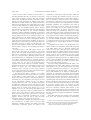
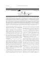
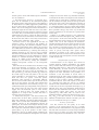
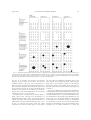
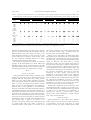
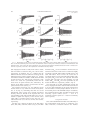
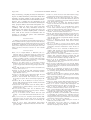
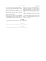
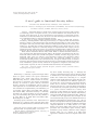
Ecological Monographs, 80(3), 2010, pp. 469–484
Ó 2010 by the Ecological Society of America
A user’s guide to functional diversity indices
D. SCHLEUTER,1 M. DAUFRESNE, F. MASSOL,
AND
C. ARGILLIER
L’Institut de Recherche en Sciences et Technologies pour l’Environnement (CEMAGREF), Unite´ de Recherche Hydrobiologie,
3275 Route de Ce´zanne, CS 40061, 13182 Aix en Provence, France
Abstract. Functional diversity is the diversity of species traits in ecosystems. This concept
is increasingly used in ecological research, yet its formal definition and measurements are
currently under discussion. As the overall behavior and consistency of functional diversity
indices have not been described so far, the novice user risks choosing an inaccurate index or a
set of redundant indices to represent functional diversity.
In our study we closely examine functional diversity indices to clarify their accuracy,
consistency, and independence. Following current theory, we categorize them into functional
richness, evenness, or divergence indices. We considered existing indices as well as new indices
developed in this study. The new indices aimed at remedying the weaknesses of currently used
indices (e.g., by taking into account intraspecific variability). Using virtual data sets, we test
(1) whether indices respond to community changes as expected from their category and (2)
whether the indices within each category are consistent and independent of indices from other
categories. We also test the accuracy of methods proposed for the use of categorical traits.
Most classical functional richness indices either failed to describe functional richness or
were correlated with functional divergence indices. We therefore recommend using the new
functional richness indices that consider intraspecific variability and thus empty space in the
functional niche space. In contrast, most functional evenness and divergence indices
performed well with respect to all proposed tests. For categorical variables, we do not
recommend blending discrete and real-valued traits (except for indices based on distance
measures) since functional evenness and divergence have no transposable meaning for discrete
traits. Nonetheless, species diversity indices can be applied to categorical traits (using trait
levels instead of species) in order to describe functional richness and equitability.
Key words: categorical variables; functional divergence; functional evenness; functional richness;
morphological traits; species richness.
INTRODUCTION
Biodiversity is commonly expressed through indices
based on species richness and species abundances
(Whittaker 1972, Lande 1996, Purvis and Hector
2000). Recently, however, studies focused on diversity
have begun to incorporate the concept of functional
diversity. In contrast to species diversity, functional
diversity measures the distribution and the range of
what organisms do in communities and ecosystems and
thus considers the complementarity and redundancy of
co-occurring species (Dı´ az and Cabido 2001, Petchey
and Gaston 2006). Functional diversity is commonly
assumed to be a better predictor of ecosystem productivity and vulnerability than species diversity (Tilman et
al. 1997, Hulot et al. 2000, Dı´ az and Cabido 2001,
Heemsbergen et al. 2004).
Including species’ functions in the measurement of
biodiversity is a relatively recent approach. Since 1990,
the number of publications based on functional diversity
Manuscript received 2 December 2008; revised and accepted
2 September 2009. Corresponding Editor: J. M. Levine.
1 Present address: Limnological Institute, University of
Konstanz, 78457 Konstanz, Germany.
E-mail: [email protected]
has been steadily increasing (Fig. 1). Although the
concept of functional diversity itself is relatively simple
to understand, its increasing importance in biodiversity
studies has revealed that measuring it is a complex
endeavor: while studies focused on species diversity only
need to count individuals from different species (i.e.,
sort them into several categories), functional diversity
studies have to describe a multidimensional cloud of
points in trait space (i.e., each coordinate corresponds to
a measured trait), each point representing an individual
or a species. Several methods have recently been
proposed to help identify the necessary measures of
functional diversity (reviewed in Ricotta 2005, Petchey
and Gaston 2006, Podani and Schmera 2007, Ville´ger et
al. 2008). Two main approaches have emerged: on the
one hand, functional groups can be defined based on few
behavioral/morphological characteristics (e.g., diet affinities, food acquisition methods, preferred habitat) and
the observed species are assigned to different functional
categories (Bremner et al. 2003, Stevens et al. 2003,
Petchey and Gaston 2006). These data can be further
processed with conventional species diversity indices
(functional group richness, Shannon index, Simpson
diversity index, etc.; e.g., Stevens et al. 2003). This
approach is suitable for macro-ecological studies since
469
470
Ecological Monographs
Vol. 80, No. 3
D. SCHLEUTER ET AL.
FIG. 1. Number of publications containing the term
‘‘functional diversity’’ in title, abstract, or key words. Source:
Scopus hhttp://www.scopus.com/scopus/search/form.urli to 31
December 2008.
information on species assignment to functional groups
is available for a broad range of species and generally
easy to obtain. Furthermore, such studies only need a
low level of detail in contrasting species traits. On the
other hand, functional diversity can be calculated based
on specific functional traits measured for each species.
This approach promises a finer resolution (Bremner et
al. 2003, Petchey and Gaston 2006), but trait values are
more difficult to obtain than information on functional
group memberships. For instance, it is easier to
categorize fish species by their general diet than to
obtain measurements on their size, gape width, stomach
length, etc. Functional traits can be morphological traits
that represent adaptations to different diets or habitats,
physiological traits (e.g., temperature tolerance), reproductive traits (e.g., number of eggs and egg diameter), or
behavioral traits (e.g., migratory behavior or parental
care) (Bremner et al. 2003, Dumay et al. 2004, Lepˇs et al.
2006). Because most of these measurements are realvalued (i.e., not discrete) and more than one trait is used
to describe the different functions, the indices commonly
used to measure species diversity cannot be applied (e.g.,
Simpson diversity index).
To make use of multiple trait measurements, Bremner
et al. (2003) compared functional trait compositions
between sites using principal components (PCA) or coinertia analyses. However, this approach is comparative
and not based on functional diversity per se and
therefore does not give absolute insight into the
distribution of traits within a specific site. Alternatively,
species diversity indices have now been transposed to
functional diversity measurements, and several new
indices have been proposed (e.g., Mason et al. 2005,
Ricotta 2005, Petchey and Gaston 2006, Ville´ger et al.
2008). These indices usually describe two broad aspects
of functional diversity: (1) how much of the functional
niche space is filled by the existing species (functional
richness) and (2) how this space is filled (functional
evenness, functional divergence/variance).
Using functional diversity indices, however, entails
several methodological problems. The first difficulty is
the selection and the treatment of the traits, e.g., how
many and which traits to use, how to weigh them, and
how to combine them (Lepˇs et al. 2006, Petchey and
Gaston 2006). Some solutions to these problems have
been discussed and proposed by Lepˇs et al. (2006). The
second set of problems is related to the indices
themselves, i.e., do the indices measure exactly what
the user wants to describe? Are the chosen indices
independent from one another? Will diversity be
measured for a single trait only or for a multivariate
trait data set? Does the data set contain categorical and
continuous variables? It is particularly important that
these problems are considered carefully because ecological theories are developed and confirmed based on these
results.
Some properties of selected indices were specified by
Petchey and Gaston (2006) and Ricotta (2005), but new
indices have been published since then (e.g., Cornwell et
al. 2006, Podani and Schmera 2007, Ville´ger et al. 2008),
and although the importance of intraspecific specialization and variability is clearly acknowledged (Bolnick et
al. 2003), it has rarely been considered in the formalization of functional diversity. Moreover, a direct comparison of the different indices and their correlations with
one another is still missing, and the user of functional
diversity still faces the problems described here when
selecting an index. The aims of this study were therefore:
(1) to describe the main properties of the different
functional diversity indices; (2) to propose new indices
that enhance and supplement existing ones (e.g.,
accounting for intraspecific variability); (3) to test and
compare the accuracy of all these indices in defined
scenarios; (4) to measure the correlations among all
these indices; (5) to summarize the results of 1–4 in a
table to facilitate the selection of an appropriate index
for the user.
METHODS
Functional diversity indices
The functional diversity of a community approached
through the measurements of traits is usually described
by three kinds of indices that can be combined to
calculate different facets of functional diversity (Mason
et al. 2005, Ville´ger et al. 2008; examples for application,
Mason et al. 2007, 2008): functional richness (FR),
functional evenness (FE), and functional divergence
(FD). The FR indices generally measure how much
niche space is filled, while FE and FD indices describe
how this space is filled. Defining functional diversity
indices, however, is not a simple task since there is no
natural way of describing richness, evenness, or divergence when individuals are not assigned to classes (i.e.,
species), but rather described by their traits. First, any
index should reflect the verbal definition of its properties. Second, FR, FE, and FD indices aim at measuring
different aspects of functional diversity and should
therefore be uncorrelated (independent) in a random
community.
August 2010
FUNCTIONAL DIVERSITY INDICES
There are nine indices available in the literature to
calculate functional diversity on the basis of measured
traits, which we describe and test in this study: three FR
indices (first described by Petchey and Gaston 2002,
Mason et al. 2005, Cornwell et al. 2006), two FE indices
(Mouillot et al. 2005, Ville´ger et al. 2008), and four FD
indices (first described by Rao 1982, Mason et al. 2003,
Lepˇs et al. 2006, Ville´ger et al. 2008). Each index group
contains one- and multidimensional indices. Despite
their multiplicity, these indices still miss some important
points, e.g., FR indices do not consider individual
variability. Indeed, individual variability in functional
diversity has been approached through the expansion of
existing indices for the use of individuals (Lepˇs et al.
2006, Cianciaruso et al. 2009). However, indices that
specifically account for the use of intraspecific variation
(using means and intraspecific variability as input, not
individual trait values) have only been proposed for two
FD indices (Lepˇs et al. 2006). To fill these gaps, we
propose three additional indices (two FR indices and
one FD index), which are also described and tested in
this study.
Functional richness.—The FR indices measure how
much of the niche space is occupied by the species
present. They are usually interpreted by ecologists as an
indicator for potentially used/unused niche space and
thus, e.g., for productivity, buffering against environmental fluctuations, or vulnerability to invasion (Mason
et al. 2005). Functional richness is naturally positively
correlated with the number of species present (the more
species there are, the larger the functional space
occupied when species traits are somewhat randomly
distributed). However, two communities with the same
number of species may have different FR when
functional traits of species are more closely clustered
in one community than in the other. Functional richness
is not weighted by species abundance.
1. One-dimensional indices.—Mason et al. (2005)
suggested using the functional range (FRR) as a measure
of FR (Table 1: index number [IN] 1.1). Functional
range is the relative range of a trait that is filled by a
community at a site compared to the range of the trait
for all communities together. In this way FRR is
restricted between 0 and 1 and becomes comparable
for differently scaled traits. Please note, however, that
the value for an individual site is not absolute but might
change when the overall range changes (e.g., by the
addition of a new site with species that differ in trait
values). The community’s range is calculated based on
species’ mean trait values by simply subtracting the
lowest from the highest mean trait value at a site. The
absolute range is calculated accordingly for all sites
together. If more than one trait is used, the mean
community range is then the mean of all traits.
Neither individual variability nor gaps in trait space
are accounted for by FRR. This is an issue when
individual variability between sites differs and when
functionally exceptional species are added to the
471
community or when species with trait values within the
range are missing. We therefore propose a new onedimensional functional richness index (FRIs) (Table 1:
IN 1.2). The FRIs is based on species’ trait variability:
instead of the community’s trait range, FRIs is based on
the union of the species’ trait ranges (and thus considers
individual variability). It is calculated as the union of
species’ trait ranges at one site, relative to the union of
species’ trait ranges for all sites together (see FRR).
When calculating FRIs the species’ trait range can be
calculated using two species/trait matrices as input
tables, containing the species’ minimum and maximum
trait values, respectively. With this method, however, the
range depends on the number of individuals measured.
We therefore suggest using more conservative values,
e.g., the 10th and 90th percentiles, confidence intervals,
or the mean species trait value 6 SD. For further details
see Appendix A. A script in R for this index is available
online.2
2. Multidimensional indices.—The multivariate counterpart of FRR is the functional volume FRV (Cornwell
et al. 2006; Table 1: IN 1.3). The FRV calculates the
volume of trait space with the convex hull volume,
which represents the smallest convex hull that encloses
all species. With a complex algorithm, the most extreme
points (vertices) can be determined and the volume
encompassed by these vertices is calculated (TraitHull
programmed in Python [Cornwell et al. 2006], available
online;3 and for R [Ville´ger et al. 2008], available online).4
To calculate this index, the number of species must
always exceed the number of traits.
A second existing multidimensional FR index is the
dendrogram-based index FRD (Petchey and Gaston
2002) (Table 1: IN 1.4). This index measures the extent
of species complementarity based on a trait distance
matrix (Petchey and Gaston 2002), a property equivalent to FR (Mouillot et al. 2005). A dendrogram is
computed by hierarchical clustering; the functional
richness is then the sum of the branch lengths of species
present. There has been discussion in the literature on
which distance measure and cluster method is best at
calculating this index (Podani and Schmera 2006, 2007,
Petchey and Gaston 2007, Mouchet et al. 2008). Here,
we used the method developed by Mouchet et al. (2008;
R program available online, see footnote 4) that
computes dendrograms based on two distance matrices
and seven clustering methods, which belong to the
family of hierarchical agglomerative classifications and
then selects the combination (including a consensus tree)
that best represents the species distribution in functional
trait space.
As for FRR, FRV does not consider gaps in functional
trait space. We therefore developed a multivariate
2 hhttp://www.cemagref.fr/le-cemagref/lorganisation/lescentres/aix-en-provence/ur-hyax/scripts/ecology_schleuter2010/i
3 hhttp://www.pricklysoft.org/software/traithull.htmli
4 hhttp://www.ecolag.univ-montp2.fr/softwarei
472
Ecological Monographs
Vol. 80, No. 3
D. SCHLEUTER ET AL.
TABLE 1. Index number (IN), index abbreviation (IA), name, formula, and references for the different functional diversity indices.
IN
IA
Name
Formula
Source
maxðXts Þ minðXts Þ
1.1 FRR
functional range
1.2 FRIs
functional richness
(one-dimensional)
s2Sc
s2Sc
Mason et al. (2005)
max ðXts Þ min ðXts Þ
s2[Sc
s2[Sc
Z
max½1st ðxÞ dx
s2Sc
Z
max ½1st ðxÞ dx
this study
s2[Sc
1.3 FRV
1.4 FRD
1.5 FRIm
2.1 FEs
where 1st(x) is 1 if x is between
min and max, else it is 0 for
categorical variables, Ltc/Lt
functional volume
the volume inside the minimum
convex hull that encloses all species
in functional space
functional dendrogram distance matrices: Euclidean, Gower;
clustering methods: single linkage,
complete linkage, UPGMA, WPGMA,
WPGMC, Ward’s method
Z UPGMC,
functional richness
max fs ðZÞ dZ
s2Sc
(multidimensional)
where fs(Z) ¼ exp[0.5(Z Xs)> R 1
s (Z Xs)]
2
functional evenness
(one-dimensional)
jSX
c j1
s¼1
Cornwell et al. (2006)
Petchey and Gaston (2002),
modified by Mouchet et al. (2008)
this study
3
7
6
6
jXtsþ1 Xts j=ðAtsþ1 þ Ats Þ
1 7
7 Mouillot et al. (2005)
min6
;
6jSX
jSc j 17
5
4 c j1
jXts 0 þ1 Xts0 j=ðAts 0 þ1 þ Ats 0 Þ
s 0 ¼1
where species subscripts, s, are ranked by
ascending order of trait value, t;
for categorical variables:
Lt
X
Al 1
;
min
A Lt
l¼1
3
2
X
6 distðeÞ=ðAe =AÞ
1 7
1
7
min6
4X distðe 0 Þ=ðA 0 =AÞ ; jSc j 15 jSc j 1
e
e2E
2.2 FEm
functional evenness
(multidimensional)
3.1 FDvar functional logarithmic
variance
3.2 FDr
functional variance
(FDvar modified)
3.3 FDcat
functional
unalikeability
3.4 FDs
functional divergence
(one-dimensional)
3.5 FDQ
Rao’s quadratic
entropy
e 0 2E
1
1
jSc j 1
Ville´ger et al. (2008)
"
!#
T X
2
2
1X
As arctan 5
ln Xts ln Xts
p
T t¼1 s2Sc A
Mason et al. (2003)
where ln Xts is the mean of ln Xts over all
species present
X As 2
Xts Xts
A
s2Sc
Lt 2
X
Al
FDcat ¼ 1 A
l¼1
Lepˇs et al. (2006)
Q1 ðYt Þ Q3 ðYt Þ
maxs2Sc ðXts Þ mins2Sc ðXts Þ
where Yt is a dummy variable that takes
values Xts with frequency As
X X As As 0
distðs; s 0 Þ
A2
s2Sc s 0 2Sc
Kader and Perry (2007)
this study
Rao (1982), Champely
and Chessel (2002)
August 2010
FUNCTIONAL DIVERSITY INDICES
473
TABLE 1. Continued.
IN
IA
Name
3.6
FDm
functional divergence
(multidimensional)
Formula
Dd þ dG
Djdj þ dG
where Dd ¼
Source
Ville´ger et al. (2008)
X As
s2Sc
A
ðdGs dGÞ,
Djd j ¼ Rs2 Sc(As/A)jdGs dGj; dGs is the distance between
species s and the gravity center of the convex hull
(coordinates Gt ¼ (1/jVj)Rs2 VXts) and dG is the
mean value of dGs over all present species
Notes: IN starting with 1, 2, or 3 and IA starting with FR, FE, or FD refer to functional richness, functional evenness, and
functional divergence index groups, respectively. Subscripts s and m of index acronyms refer to single (one-dimensional) or
multidimensional indices. Abbreviations: i, s, c, l, and t are individual, species, community, level of trait (for categorical variables),
and trait subscripts, respectively; As, abundance of species s; Ats, abundance of species s when species are sorted following trait t
ascending ranking; A, total abundance of all individuals; Al, abundance of trait level l; Is, set of individuals of species s; Ltc, number
of levels of categorical trait t covered by community c; Lt, total number of levels of trait t; L, total number of cross-trait levels; Sc,
set of species present in community c (jScj, number of species present in community c); T, number of traits studied; Vc, set of vertex
species from the convex hull in community c (jVcj, the corresponding number of vertices); xtsi, value of trait t in individual i from
species s; Xts, mean value of trait t in species s; Xs, mean value of all traits in species s arranged in a vector; Z, sample vector of all
traits, used for the purpose of computing integrals over trait space; R, variance/covariance matrix of traits; dist(s, s 0 ), distance
between species pairs based on mean trait values (for continuous variables, Euclidean distance is used; for discrete variables, the
Gower distance is used); E, set of edges connecting species pairs in the minimum spanning tree; e, subscript of an edge; dist(e),
distance between endpoint species of edge e; Ae, sum of the abundances of the endpoint species of edge e; Q1, lower quartile; Q3,
upper quartile; UPGMA, unweighted pair group method using arithmetic averages; WPGMA, weighted pair group method using
arithmetic averages; UPGMC, unweighted pair group centroid method; WPGMC, weighted pair group centroid method.
counterpart to FRIs: FRIm (Table 1: IN 1.5). The FRIm
index is specifically designed to account for individual
variability and for gaps in the multidimensional
functional trait space. The idea is to compute an
equivalent ‘‘range union’’ (as for FRIs) across species
present in a community. To do so, each species s is
assigned a function on trait space ( fs) that indicates
whether a particular point in trait space is (or is not)
occupied by species s (that is, whether species s trait
values encompass this point). Here, we chose a simple
form for fs functions that uses information on both
mean trait values and trait variance–covariance matrices
for each species. FRIm is then obtained as the integral of
the maximum of all fs functions (integrated over studied
trait space). For further details see Appendix B. A script
in Mathematica to calculate this index is available online
(see footnote 2).
Functional evenness.—Functional evenness indices
measure whether mean species traits are distributed
regularly within the occupied trait space, i.e., with equal
distances between nearest neighbors and equal abundances (a high FE index usually means a very regular
distribution; a low FE index indicates the existence of
separate clouds of species and/or abundances). Functional evenness indices are generally used to indicate
under- or overutilization of resources and thus again
productivity, reliability, and vulnerability to invasion
(Mason et al. 2005). This index group includes species’
abundances in its calculation.
1. One-dimensional index.—Based on Bulla’s index
for the measurement of species’ evenness (Bulla 1994),
the FEs index (Mouillot et al. 2005) measures for each
trait separately how evenly the trait values of all species
present are distributed (Table 1: IN 2.1). First, the
absolute, relative distances between the mean species
trait values, in order of increasing values, is calculated
and weighted by the sum of the relative species
abundances. Second, if the distance is greater than 1/
(S 1) (with S representing species richness), it is
replaced by 1/(S 1), the distance, which is obtained for
an optimal even distribution (Mouillot et al. 2005). FEs
is 1 if the distance between nearest neighbor species is
exactly 1/(S 1) and all species have the same
abundances. The more a community differs from the
optimal distribution in terms of abundance and trait
difference, the lower the FEs. When trait space is
multidimensional, the community’s evenness is the
average of the FEs calculated for each trait.
2. Multidimensional index.—The multivariate equivalent of FEs is FEm (Ville´ger et al. 2008; Table 1: IN 2.2).
Instead of using the absolute distances between the
species’ trait values for each trait separately, this index
uses the abundance-weighted distances between all
species pairs to calculate first the minimum spanning
tree (MST) that links all the species in a multidimensional trait space. The index then measures the
regularity of the MST branch lengths, according to
FEs (i.e., comparison with the optimal branch length
distribution).
Functional divergence.—The FD indices, finally, measure the variance of the species’ functions and the
position of their clusters in trait space (a high FD is
caused by the clustering of species and/or abundances at
the edges of the traits’ space). The FD indices find
application for indicating the degree of resource
differentiation and thus competition (Mason et al.
2005), but they can also indicate a predominance of
474
D. SCHLEUTER ET AL.
extreme species. As FE, FD includes species’ abundances in its calculation.
1. One-dimensional divergence.—Functional divergence can be calculated as the abundance-weighted
functional variance using mean species values (Mason et
al. 2003). Mason et al. (2003) suggested log transforming
the trait values before calculating the variance (FDvar;
Table 1: IN 3.1) and using species relative abundances as
abundance weight. If more than one trait is used, FDvar
is calculated for each trait separately and then averaged
over traits. They recommend then using an arctangent
transformation in order to restrict the index between 0
and 1. If species and/or abundances are clustered around
the mean trait value, FDvar is low; if they are clustered at
the edges of the community, FDvar is high.
The FDvar index is not applicable if the data set
contains 0 values. To account for this problem, we
propose using simply the abundance-weighted variance
without log transformation (FDr; Table 1: IN 3.2) (Lepˇs
et al. 2006). Since the variance is scale-dependent, traits
should be standardized (e.g., centering and scaling by
standard deviation) in case the trait space is multidimensional and the different traits have different scales.
Another possibility is to use the coefficients of variation
instead (i.e., standard deviations divided by means).
Lepˇs et al. (2006) suggest including intraspecific
variability in this index by adding the abundanceweighted intraspecific variance to the interspecific
variance.
Since FD can also be understood as the relative range
of the trait clustering, we propose a new one-dimensional index of functional divergence, FDs. The FDs
index calculates the range of the zth percentiles (e.g.,
25th percentile, Q1, and 75th percentile, Q3) relative to
the overall range of each trait (Table 1: IN 3.4). The
species abundance is accounted for by replicating the
mean trait value of a species i times the species’
abundance. This approach is conceptually different,
since it is based on the relative span of the trait cluster
and not on the variance. Low FDs values indicate that
half of the individuals in the community occupy a very
confined functional space, independent of the position of
that cluster along the trait axis; high values instead
suggest that the functional space is more densely
occupied at both its edges. For further details see
Appendix C. A script in R to calculate this index is
available online (see footnote 2).
2. Multivariate divergence.—The most common multivariate index of FD is Rao’s quadratic entropy FDQ
(Rao 1982, Champely and Chessel 2002, Ricotta 2005;
Table 1: IN 3.5). This index calculates the abundanceweighted variance of the dissimilarities between all
species pairs. It is based on the Simpson diversity index
(Simpson 1949) for the calculation of species diversity
and weighs the trait-based distances between pairs of
species [dist(s, s 0 )] by the product of their relative
abundances. Lepˇs et al. (2006) suggest calculating the
species’ pairwise dissimilarities through the sum of their
Ecological Monographs
Vol. 80, No. 3
overlaps for each trait. In this way, individual variability
is included in this index and categorical and continuous
variables can be mixed. Rao’s quadratic entropy can
also be calculated for single traits, the average of which
leads to the same result as the multivariate approach, if
the distance measure used is unchanged by averaging
(e.g., Euclidean distance; Lepˇs et al. 2006). Since Walker
et al.’s (1999) functional attribute diversity differs from
Rao’s quadratic entropy only in the way the distance
matrix is calculated, it was not tested as a separate index
in this study.
Ville´ger et al. (2008) proposed a new multivariate
measure for functional divergence (FDm). Based on the
vertex species V of the convex hull (see FRv), this index
first determines the center of gravity G of the convex hull
(Table 1: IN 3.6). It then computes the abundanceweighted deviances Dd of each species present from the
species’ mean distance to the center of gravity. In a last
step, the index is restricted between 0 and 1. The FDm
index is low when species/abundances are close to the
center of gravity and high when species and/or
abundances are higher at the vertices of the convex
hull. Since this index is based on the calculation of the
convex hull, the same assumptions as for the calculation
of FRV must be met.
Transformation of trait data
Transformations of the original data should be
avoided whenever possible. Nonetheless, one should
always consider that some indices are not applicable to
differently scaled traits (e.g., FDr). If at least one trait is
scaled differently, all traits should be transformed;
otherwise, this trait might have too little or too much
weight in the index calculation. One possibility is to
transform a trait that differs in several orders of
magnitudes from the others using an algebraic function
such as the logarithm (e.g., number of seeds in plants or
number of eggs in fishes). Another possibility is to
standardize the trait values with respect to the others,
e.g., centering and scaling the trait by its standard
deviation. This transformation has to be done for the
overall data set and not on potential subsamples (e.g., at
different study sites). The subsamples should then be
drawn from the transformed trait matrix. For indices
that calculate relative index values for each trait
separately (e.g., FRR, FRIs, FDs, etc.) and for onedimensional indices, which range between 0 and 1 (e.g.,
FEs, FDvar), the data need not to be transformed.
Different transformation methods and their pros and
cons are summarized in Lepˇs et al. (2006).
Accuracy of the indices
The first criterion for the quality of an index
(accuracy) is the match between the way it actually
behaves and the verbal definition of its properties (FR,
FE, FD). This was tested in our study using an artificial
data set (up to 25 species, two traits). We manipulated
species composition and abundances in five tests (T1–
August 2010
FUNCTIONAL DIVERSITY INDICES
475
FIG. 2. Illustration of the artificial scenarios used to test the behavior of the different indices. There are five different tests (T1–
T5) whereby an initial community is modified three times in different ways (scenarios a–c). Each square represents one community
with two trait axes; one dot within a square represents a species. The size of the dot indicates the abundance of the species (small
dots reflect one individual, and with increasing size, 2, 25, and 250 individuals).
T5; Fig. 2) to compare the observed and expected
changes of index values. Trait values were integer
numbers between 1 and 5 for trait 1 and between 1
and 8 for trait 2. We assumed a standard deviation of 0.2
and a maximum deviation from the mean equal to 0.4
for all species and traits. In all tests, the initial species
richness was 25, apart from T1, where it was 24. In T1
and T2 and, if not stated differently, in T3–T5, species
abundance was set to 1 for all species.
The main aim of T1 and T2 was to test the effect of
empty space in the trait space on the behavior of
functional richness indices. In T1, we tested the effect of
adding one species, with varying distance between the
added species and the existing community (Fig. 2, T1).
In T2, we removed nine species from the initial
community. We removed these species so that either
one trait value was eliminated completely, once at the
outer edge of the community and once within the trait
space (Fig. 2, T2 scenarios a and b), or the removed
species were chosen in the middle of the trait space so
that each trait value was present at least once (Fig. 2, T2
scenario c).
In T3–T5, the influence of varying species abundances
on functional evenness and divergence was tested. In T3,
we increased the abundance of one species stepwise from
1 (initial community) to 2, 25, and 250 individuals to test
for the influence of the change in the abundance of one
species (Fig. 2, T3). In T4, the influence of the position
in trait space of a dominating species (25 individuals)
was tested (Fig. 2, T4). In T5, we increased the distance
between two dominating species (25 individuals each),
starting from an initial community in which the
476
D. SCHLEUTER ET AL.
abundance of only one species was set to 50 individuals
to simulate two identical species.
All indices were calculated for the initial community
and for the different scenarios. The change in index
values of the scenarios compared to the initial community was evaluated semi-quantitatively. We used the
symbols ‘‘,’’ ‘‘þ,’’ and ‘‘¼’’ to indicate whether the
calculated value was higher, lower, or equal, respectively, compared to the initial community. The symbols
were replicated to give a raw quantitative view of the
changes (þþ, þþþ with þ,þþ,þþþ; , with
, ,).
Indices correlation
The correlations among the different indices were
tested using random communities. We computed 1000
randomizations for 14 different species richness levels
(as multiples of five from five to 70) and three different
numbers of traits (three, five, 10). The total number of
treatments was 42 (14 3 3). Trait values were generated
using uniform distributions between 0 and 1. The
intraspecific standard deviation was considered to be
10% of the randomized trait value. Species abundances
were randomized with a uniform distribution between 1
and 100 for each randomized trait matrix.
All indices described were calculated for each of the
42 000 random communities, apart from FRIm, which
was only calculated for the three-trait simulation.
Actually, its computation time was very long on the
computers used in this study, and it increased exponentially with the number of traits used.
To provide an overview of the relationships between
different community indices, we used ordination techniques (e.g., PCA), which are known to perform well
when summarizing complex data (Lebart et al. 2000).
Since we had to compare a set of 42 matrices of 1000
rows (randomized communities) and 12 columns (indices), a single matrix-based approach was not appropriate. As a consequence, for each of the three trait levels,
we used a multi-table ordination technique (e.g.,
Escofier and Pages 1994, Lavit et al. 1994, Chessel and
Hanafi 1996) to assess the common structure of the 14
species richness-specific matrices. We performed a
STATIS analysis (Lavit et al. 1994) to summarize the
link between the different indices while removing the
potential effect of species richness. This method is based
on the optimization of the average ordination of the
species richness-specific ordinations. The first step of
STATIS consisted of calculating a matrix of scalar
products between indices for each of the 14 levels of
species richness. In a second step, the 14 rows 3 14
columns matrix of the pairwise vectorial correlation
coefficients (RV coefficients) between the scalar products’ matrices was computed. The RV coefficient ranges
from 0 to 1 and evaluates the extent to which two
matrices share a common structure (Robert and
Escoufier 1976). Then the matrix of RV values was
diagonalized and the 14 coefficients of the first
Ecological Monographs
Vol. 80, No. 3
eigenvector were used to weight the 14 matrices of the
scalar product between indices. A mean table of
maximum inertia (called the reference structure) was
subsequently computed as the weighted sum of the
matrices of the scalar product between indices. By
weighting the sum, greater importance was given to
tables with similar structures, whereas lesser importance
was given to the other tables. Finally, a PCA was
performed on the reference structure. It provided the
graphical representation of the common structure of the
indices derived from the 14 species richness-specific
tables.
Two groups of statistics synthesized the relevance and
the efficiency of STATIS. The first statistics were the RV
coefficients between two species richness-specific tables.
The second statistical procedure used was the squared
cosines (cos2) of the angles between the first axis scores
of separate PCAs performed on each species richnessspecific table and the first axis scores of the reference
structure. This evaluates the match between the species
richness-specific tables and the reference structure by
using synthetic auxiliary variables.
Categorical variables
All the indices proposed so far (except those based on
a distance matrix) cannot be computed for categorical
variables. To address this problem, it is recommended in
the literature to transform the data set from categorical
to continuous variables via distance matrices and
ordination methods, which allow a mix of continuous
and categorical variables as inputs. Ville´ger et al. (2008)
proposed calculating the Gower distance and then
computing a principal coordinate analysis (PCoA).
The trait values thus transformed (principal coordinate
axis) can then be used to calculate the different
functional diversity indices. Next to using the Gower
distance with a PCoA, Hill and Smith’s method can also
be used (Hill and Smith 1976). This ordination
technique combines discrete and continuous variables
in a single analysis. If all variables are discrete, it is
reduced to a simple correspondence analysis.
Although it is not really correct to transform
categorical traits to continuous ones for the use of
indices designed for real-valued variables, we consider
these methods because they are commonly applied.
Since continuous trait-based indices cannot be calculated for categorical traits it is impossible to assess the true
effect of the transformation on the outputs (i.e., to
compare the outputs for transformed and untransformed trait values). As a consequence, we only
pseudo-tested the effects of these transformations using
continuous traits as input. In this way, the normally
calculated indices can serve as a reference value. As
described above, we computed 1000 randomizations for
six different species richness levels (in multiples of 10
from 10 to 60) with three traits. We then calculated all
indices (1) with the original data set, (2) with the data set
transformed via the Gower distance and PCoA (Podani
August 2010
FUNCTIONAL DIVERSITY INDICES
477
TABLE 2. Results for the five index tests, T1–T5 (as illustrated in Fig. 2): expected changes for the index categories (boldface) and
observed changes of index values for the different scenarios compared to the initial community and in relation to one another.
T1
Index
T2
T3
T4
T5
a
b
c
a
b
c
a
b
c
a
b
c
a
b
c
Richness
FRR
FRIs
FRV
FRD
FRIm
þ
¼
¼
¼
þþ
þ
þ
þ
þ
þ
þ
þ
þ
þþ
þ
þþ
þ
¼
¼
¼
¼
¼
¼
¼
¼
¼
¼
¼
¼
¼
¼
¼
¼
¼
¼
¼
¼
¼
¼
¼
¼
¼
¼
¼
¼
¼
¼
¼
¼
¼
¼
¼
¼
¼
¼
¼
¼
¼
¼
¼
¼
¼
¼
¼
¼
¼
¼
¼
¼
¼
¼
¼
¼
¼
¼
¼
Evenness
FEs
FEm
þ
¼
¼
þ
þ
þ
þ
þþ
¼
¼
¼
¼
¼
¼
¼
þ
¼
þþ
þ
¼
Divergence
FDvar
FDr
FDs
FDQ
FDm
¼
þ
þ
þ
þþ
þþ
þþ
þ
þ
þ
þ
þþ
þ
þ
þþ
þþ
þþ
þþþ
þþ
þþ
¼
þ
þ
þ
þ
þ
þ
þþ
þþ
þþ
þþ
þþ
þþ
þþþ
þþþ
þþþ
þþþ
þþþ
þþþ
þ
þ
þ
þ
þ
þ
þþ
þþ
þþ
þþ
þþ
þþ
þþþ
þþþ
þþþ
þþþ
þþþ
þþþ
Notes: Symbols are: , lower than initial community; þ, higher than initial community; ¼, no change. The number of þ and signs indicates the increase compared to the other scenarios. See Table 1 for explanations of indices.
and Schmera 2006, Ville´ger et al. 2008), and (3) with the
data set transformed using Hill and Smith’s method
(Hill and Smith 1976). The common structure of the
three calculation methods was then assessed for each
species richness level separately, using the RV values
(i.e., the correlation coefficient between two tables)
obtained from the method-specific tables.
All calculations and tests were carried out using the
program R (R Development Core Team 2008). The
STATIS analysis and the transformation via the Hill
and Smith method and PCoA were computed using the
ade4 package (Chessel et al. 2004, Dray et al. 2007).
RESULTS
Accuracy of the indices
Testing whether the indices behave according to the
properties of the index group to which they have been
assigned (FR, FE, FD) reveals that, among the FR
indices, only two of them (FRIs and FRIm) accurately
reflect the expected changes in functional richness (see
Table 2: T1 and T2), because these indices consider
empty space in the trait distribution of a community.
However, FRIs is only applicable to one-dimensional
situations, while FRIm well reflects functional richness in
a multidimensional space. The results from scenario T1 c
and scenarios T2 a and b show that when one trait value
is missing in the entire data set, both indices decrease.
However, in a multidimensional space, when none of the
trait values of the removed species are unique, but their
combination is, FRIm is the only index that reflects these
gaps properly (Fig. 2, Table 2: T1 scenario a, T2
scenario c). In contrast, indices such as functional range
or volume (FRR, FRV ) only reflect a decrease in
functional richness when species are removed at the
edge of the community. The dendrogram-based index
for functional richness, FRD, is furthest from the
expected results for functional richness.
Among the two FE indices, the multivariate index
FEm behaves more adequately than its one-dimensional
counterpart FEs and matches the expected results quite
well. Thus, FEm can be considered an appropriate index
(Table 2). However, this index fails to respond
adequately in some cases, for example when species in
the center of the community are added or subtracted (T1
scenario a and T2 scenario c). Species traits are then not
evenly distributed over the entire functional space, but
concentrated at the edges of the community, and thus
the evenness is theoretically lower than in the initial
community. Yet FEm remains equal because the
distribution of the branch lengths of the minimum
spanning tree (the distance to the nearest neighbors)
does not change. The one-dimensional index FEs does
not represent the distribution of species in a multidimensional trait space, but it reflects the evenness of the
distribution for a single trait well (results not shown)
and can be used if only one trait is considered.
All FD indices adequately match expectations. Even
one-dimensional indices, averaged over all traits, accurately reflect changes in a multidimensional space (Table
2). Only in T1 do FD indices react differently: as
expected, FDr and FDvar increase when a species
outside of the initial community is added, whereas
FDQ, FDm, and FDs decrease.
Indices correlation
Species richness has a clear effect on the different
indices, either in terms of variance or mean values (Fig.
3). Nevertheless, for all trait levels, there is a high
similarity between the species richness-specific tables
478
D. SCHLEUTER ET AL.
Ecological Monographs
Vol. 80, No. 3
FIG. 3. Relationship of each of the 12 functional diversity indices with species richness (SR; 14 levels from 5 to 70), here for a
data set with three different species traits. There are 1000 index values for each species richness level based on randomized trait and
abundance data. Trait values and species abundances were generated using uniform distributions between 0 and 1 and between 1
and 100, respectively. See Table 1 for explanations of functional diversity indices.
(RV ranging from 0.885 to 0.996, from 0.945 to 0.998,
and from 0.962 to 0.998 for three, five, and 10 traits,
respectively). In addition, the cos2 confirms that the
different reference structures reflect the structures of the
individual species richness-specific tables (cos2 ranging
from 0.905 to 0.944, from 0.920 to 0.940, and from 0.924
to 0.941 for three, five, and 10 traits, respectively). The
lowest cos2 values are systematically found for the
lowest levels of species richness (five, followed by 10)
because of the higher variance of most indices at these
species richness levels (see Fig. 3).
The reference structures over the different species
richness levels are very similar for all trait levels (three,
five, or 10; Fig. 4), confirming that there are several
independent index groups that describe functional
diversity. However, instead of the expected three axes
corresponding to FR, FE, and FD indices, five axes are
needed to explain the majority of the variance (74%)
when FRIm is included (three traits) and four axes
without this index (77% and 78% for five and 10 traits,
respectively).
The first axis is mainly correlated to the FD indices
(FDr, FDs, FDQ, and FDm; Table 3, Fig. 4). The fifth
FD index (FDvar) is also correlated to the first axis, but
with the second axis as well and it is overall more highly
correlated to the FR indices FRR and FRV than to the
other FD indices. Next to FDvar the second axis is
correlated mainly to some of the FR indices (FRR, FRV,
and partly FRIs). The third axis represent functional
evenness (FEs and FEm) and the remaining two FR
indices (FRIm and FRD) are best represented by the
fourth and fifth axes, respectively (Table 3, Fig. 4).
Note that FRV is not fully independent of FDQ and
FDs (r ranging from 0.09 to 0.59 for FDs and from 0.21
to 0.71 for FDQ depending on the species richness level
and the number of traits), despite distance in the F1 3
F2 factorial plane of the STATIS analysis. In addition,
the correlation between FRIs and FRIm decreases with
increasing species richness (from r ¼ 0.61 in a
community with five species to r ¼ 0.00 in a community
with 25 species).
Categorical variables
One- and multidimensional indices react differently to
the transformation from discrete to continuous variables. Therefore, correlations between the method-
August 2010
FUNCTIONAL DIVERSITY INDICES
479
FIG. 4. Reference structures over the different species richness-specific ordinations gained from the STATIS analysis (Lavit et
al. 1994). (a) Reference for three traits, first and second axes; axis 1 mainly correlates with FD indices, while axis 2 with FR indices.
(b) Reference for three traits, third and fourth axes; the third axis mainly correlates with the two FE indices, axis 4 represents FRIm.
(c) Reference for five traits, first and second axes; axis 1 mainly correlates with FD indices, while axis 2 correlates mainly with FR
indices. (d) Reference for 10 traits, first and second axes; axis 1 mainly correlates with FD indices, while axis 2 with FR indices. The
insets display the eigenvalues (here expressed as percentage of contribution for the explanation of the variance, y-axis) of each axis
(ordered from 1 to 12, x-axis). Shading of the bars refers to the importance of each axis, whereby white bars can be considered as
statistical noise. The d values give the scaling of the grid. See Table 1 for explanations of functional diversity indices.
specific tables (RV values) have been computed separately for these two index groups. For multidimensional
indices, we have found a high similarity between the
index tables calculated with the raw data and the
differently treated data sets. The transformation via the
Hill and Smith method performs slightly better (RV
range dependent on species richness between 0.897 and
0.956 for Gower distance and PCoA transformed data
and between 0.997 and 0.999 for data transformed with
the Hill and Smith method). That the results were worse
for the transformation via the Gower distance and
PCoA is mainly imputable to the calculation of FRV (r
with the index calculated with untransformed values
ranged from 0.13 to 0.60, depending on species richness)
and FDQ (r ; 0.5).
For the one-dimensional indices, neither of the
transformation methods performs well (RV ranging
between 0.605 and 0.894 for the transformation via
480
Ecological Monographs
Vol. 80, No. 3
D. SCHLEUTER ET AL.
TABLE 3. Axis coordinates of the different functional diversity indices for the first five axes of the
reference structure calculated with STATIS (Lavit et al. 1994) over the different species richness
levels (here for a data set with three traits).
Index
Axis 1
Axis 2
Axis 3
Axis 4
Axis 5
Richness
FRR
FRIs
FRV
FRD
FRIm
0.30
0.18
0.50
0.15
0.05
0.72
0.41
0.56
0.2
0.11
0.08
0.29
0.03
0.26
0.21
0.06
0.15
0.24
0.19
0.76
0.09
0.50
0.16
0.65
0.01
Evenness
FEs
FEm
0.04
0.05
0.05
0.00
0.71
0.64
0.21
0.26
0.17
0.19
Divergence
FDvar
FDr
FDs
FDQ
FDm
0.54
0.58
0.72
0.80
0.63
0.43
0.36
0.24
0.22
0.37
0.20
0.04
0.04
0.04
0.01
0.35
0.05
0.10
0.08
0.01
0.19
0.13
0.05
0.04
0.06
Note: Values lower than 0.4 or higher than 0.4 are boldface. For 1000 communities species
richness trait values and species abundances were generated using uniform distributions between 0
and 1 and between 1 and 100, respectively. See Table 1 for explanations of indices.
Gower distance and PCoA and between 0.688 and 0.897
for transformation via the Hill and Smith method).
DISCUSSION
Performance of the indices
The functional diversity indices described and tested
in this study performed quite differently. The quality of
the indices aimed at describing the same aspect of
functional diversity differed markedly, especially within
the group of the FR indices.
In our view, the main criterion for the selection of an
index is whether it accurately measures what it is
intended to describe. This was the case for all FD
indices, irrespective of whether they were one- or
multidimensional, as well as for the two FE indices.
However, while the multidimensional index FEm performed quite well in describing the evenness in the twodimensional space, its one-dimensional counterpart FEs
was only able to measure evenness when a single trait
was considered. In contrast, the FR indices differed
most strongly in their quality: the only indices that
reflected the expected changes in FR, when species were
removed within the functional trait space, were the two
indices that consider gaps in the functional trait space
(FRIs and FRIm). The FRR and FRV indices only partly
reflected what is considered functional richness (only if
there was a continuously filled trait space and species
were removed or added at the edges of the community),
while the results obtained from the index FRD did not
match the expected values. This index may work in some
cases (Petchey and Gaston 2006), but it failed to pass the
tests proposed here, perhaps due to the number of traits
and/or the number of species used. The behavior of this
index is thus difficult to understand, and we suggest
rethinking its interpretation.
These results were confirmed by the multi-table
ordination analysis (STATIS): instead of three principal
component axes, which were expected to correspond to
the three index groups FR, FE, and FD, we found that
five axes were needed to explain most of the variance:
three for FR and one for FD and FE. That three axes
were needed to explain the variance of FR indicates that
the existing FR indices describe independent aspects of
functional diversity: FRR and FRV form one group,
which describes the traits’ range/volume; FRIm measures
the occupation and span of trait space; FRD, which
represents the branch length of a dendrogram, is
independent of the other FR indices, but what it
actually measures is difficult to determine. The FRIs
index was not represented by a single axis, but was
partly correlated with FRR, FRV, and FRIm, because
FRIs accounts for gaps in trait space (as FRIm) but fails
to take into account the multidimensional nature of trait
space, so that gaps are severely underestimated when the
number of traits is high.
The second criterion for the selection of an adequate
index is that the chosen index is independent of indices
describing other aspects of functional diversity. This
criterion is met by the two FE indices, but not by all the
FR and FD indices: FRR and FRV both correlated with
FDvar and FRV also correlated with FDs and FDQ
(Table 4). This strongly suggests that FDvar, FRR, and
FRV rather measure a mixture of functional richness
and divergence.
Ricotta (2005) gave several other criteria for an index
of functional diversity, which are only applicable to FR
indices. For instance, an index should not decrease when
a species is added (the monotonicity criterion) or should
not increase when exactly the same species is added (the
twinning criterion). These two criteria were also tested in
August 2010
FUNCTIONAL DIVERSITY INDICES
481
TABLE 4. Indices of functional diversity tested in this study, their properties, correlation with other indices, and their
disadvantages.
Index
Source
Functional richness
FRR Mason et al.
(2005)
Description
Use
Cor. Cor. with indices
A with cat. with
from other
MD incl. variables SR
categories
functional range
no
no
yes
yes
FDvar
FRIs
this study
individual’s
functional
range
no
no
yes
yes
FRV
Ville´ger et al.
(2008)
functional
volume
yes
no
no
yes
FDvar, FDs,
FDQ
FRD
Petchey and
Gaston
(2002)
this study
sum of branch
length of
classification
functional
integral
yes
no
yes
yes
yes
no
no
yes
no
yes
yes
no
yes
yes
yes
no
no
yes
yes
no
FRR, FRV
no
yes
yes
no
no
yes
no
no
yes
yes
yes
no
yes
yes
no
FRIm
Functional evenness
Mouillot et al. evenness of trait
FEs
(2005)
values
FEm Ville´ger et al. evenness of mini(2008)
mum spanning
tree branch
lengths
Functional divergence
logarithmic varFDvar Mason et al.
(2003)
iance of traits
variance of traits
FDr Lepˇs et al.
(2006)
this study
relative range
FDs
of the distributional center
FDQ Rao (1982),
variance of
Champely
distances beand Chessel
tween species
(2002)
FDm Ville´ger et al. mean deviation
(2008)
of the distance
of the center
of gravity
Disadvantage
IN
no consideration
of gaps,
one-dimensional
one-dimensional,
intra-specific
trait variation
needed
no consideration
of gaps, SR has
to exceed
N traits
difficult to
interpret, long
computation time
long computation
time, intraspecific trait
variation needed
1.1, 1.2 (cat.)
one-dimensional
1.2., 1.2 (cat.)
1.3
1.4
1.5
2.1
2.2
no 0 values possible 3.1, 3.3 (cat.)
3.2, 3.3 (cat.)
FRV
3.4
FRV
3.5
SR has to exceed
N traits
(see FRV )
3.6
Notes: The table can be used to choose an index for the data set in question (dimensionality, type of variable, correlation with
indices of a different category). Abbreviations are: A, abundance; Adapt., adaptation; cat., categorical; Cor., correlated; IN, index
number; MD, multidimensional; N, number; SR, species richness. See Table 1 for explanations of indices.
the scenario test (Fig. 4, Table 2) and complied well with
nearly all FR indices except FRD.
In this study, we restricted our tests to classical
versions of the indices without specific patterns of data
distribution such as skewness. It would be of further
interest to include hypotheses on the data randomizations and test how variations of a certain index (e.g.,
selection of the distance measure used in FDQ ) react
under certain circumstances. However, we only expect
slight fine-tuning and not fundamental deviations from
the results presented here.
The use of categorical variables is problematic since
most tested indices can only be applied to continuous
variables. However, our pseudo-test with only continu-
ous variables already revealed that the two transformations proposed (Gower distance followed by a PCoA
and the Hill and Smith method) led to a loss of
information. When tested for multivariate traits, this
was especially true for the Gower distance transformation method followed by a PCoA; for one-dimensional
indices, both index matrices calculated on the basis of
transformed data correlated only weakly with the matrix
based on the untransformed traits. This effect might be
even worse when real discrete variables are included in
the data set. In this case, the transformation methods via
ordination techniques may not be the best choice for the
treatment of categorical variables. One way to overcome
this problem could be to use a multivariate index based
482
D. SCHLEUTER ET AL.
on a distance matrix (e.g., FDQ ) and to transform the
trait matrix only via the Gower distance (Podani and
Schmera 2006). Since the second transformation step
(the ordination technique) is missing in this approach,
we expect less loss of information. Another possibility is
the approach suggested by Lepˇs et al. (2006), who
recommend calculating dissimilarity between species
pairs via the sum of their overlaps for each trait
(continuous and categorical). In both approaches
(Gower distance and summed overlaps), continuous
and categorical variables share the same meaning and
indicate just to which extent two species are identical.
Otherwise, discrete variables cannot be transformed
to continuous variables and processed further with
indices designed for this type of variable since functional
evenness and divergence have no transposable meaning
for discrete traits (i.e., no spatial evenness and divergence of discrete variables, but evenness or variability of
trait-level distribution). Since categorical and realvalued variables are of completely different character,
it is difficult to find an index in which they can be mixed
up (for an exception see Material and methods:
Functional diversity indices: Functional divergence: Multivariate indices: FDQ ). A second approach would
therefore be to use indices aimed at measuring the
specific properties of categorical variables. At present,
we propose using the (one-dimensional) indices (as
follows) designed to calculate species diversity, using
trait levels instead of species.
The FR index (relative richness of trait levels).—
Corresponding to the relative species richness at a site,
we suggest using the number of trait levels present at a
site as a proportion of the number of trait levels for all
communities together (see FRIs; Table 1: IN 1.2).
The FE index (evenness of trait-level distribution).—
We suggest using Bulla’s index of species’ evenness
(Bulla 1994) based on the contribution of a trait level
(Al) to the overall sample size A (total number of
individuals) (see FEs; Table 1: IN 2.1).
The FD index (variability of trait-level distribution).—
We suggest using the ‘‘index of unalikeability’’ FDcat by
Kader and Perry (2007; Table 1: IN 3.3), which
corresponds actually to the Simpson index of species
diversity (Simpson 1949) but uses trait levels instead of
species. The FDcat represents the proportion of possible
comparisons, which are unalike, by calculating the
contribution of a factor level (Al) to the overall sample
size A and subtracts the sum of the squares from 1.
Note that for categorical variables, FE and FD
measure approximately the same thing, since both reflect
the equitability of distribution (Smith and Wilson 1996).
The proposed and other indices on species diversity have
been extensively tested (e.g., Washington 1984, Smith
and Wilson 1996, Beisel et al. 2003).
Recommendations for users
Based on the criteria discussed above and the tests
performed, we recommend using the multidimensional
Ecological Monographs
Vol. 80, No. 3
index FRIm to measure FR or FRIs if only a single trait
is considered. Both indices account for intraspecific
variability and consider the existence of empty space
within the functional trait space and therefore reflect the
true functional richness of the community better.
Besides, these indices are orthogonal to FE and FD
indices. If the user decides to compute FR through FRV,
the data set should not be transformed, even in the case
of differently scaled traits, since the convex hull
calculated with transformed data does not properly
represent the functional richness for geometrical reasons, but correlates negatively with the expected results
and the other indices for functional richness (results not
shown).
The FR indices are naturally correlated to species
richness. When indices of different communities are
compared with one another or when differences between
communities are explained with predictor variables, the
effect of species richness should therefore be removed
from the observed pattern, in order to describe patterns
of pure functional diversity. Since the observed relationships are not simply linear and differ between the
FR indices and because of unequal variances, we
recommend using null models to remove the effect of
species richness rather than using the residuals from a
constructed model (method, Gotelli and Graves 1996;
example for application, Mason et al. 2007, Prinzing et
al. 2008).
Both FEs and FEm can be used to calculate FE. The
use of FEs is, however, narrowly restricted to onedimensional data sets. Similarly, we cannot recommend
the use of a specific FD index because all indices reflect
the expected changes well, irrespective of whether they
are one- or multidimensional. However, it should be
remembered that not all FD indices are independent of
FR indices (Table 4), seemingly because FDvar and some
FR indices measure a mixture of FR and FD properties.
Further, it should be mentioned that indices based on a
distance matrix allow for the use of categorical and
continuous variables simultaneously, and they can
include intraspecific variability when calculated via the
pairwise trait overlap as suggested by Lepˇs et al. (2006).
Specific disadvantages of all indices are further summarized in Table 4.
Concerning categorical variables, we recommend at
present avoiding their use, if possible, or using indices
based on a distance matrix or the one-dimensional
indices of species diversity (Table 1: IN 1.2, 2.1, 3.3). In
this case, however, the user should keep in mind that the
indices designed for categorical variables (especially for
FE and FD) do not have the same meaning as their
continuous counterparts. The results for the different
traits should therefore be averaged over continuous and
categorical variables separately, rather than directly
averaged over all traits.
In real world measurements, the user comes to face
more problems apart from choosing the right index,
August 2010
FUNCTIONAL DIVERSITY INDICES
many of which (e.g., weighing of traits) are discussed in
Lepˇs et al. (2006) and Petchey and Gaston (2006). One
frequently occurring problem is that normally not all
trait values can be measured for each individual. This is,
however, not a problem for the calculation of the
indices, since the calculation of all indices (including the
newly proposed indices that include intraspecific variability) is based on mean trait values and their
variability. And how many individuals should be
measured for each species? In general the more, the
better. However, to restrict sampling effort, a reference
value could be the amount of individuals that are
necessary to describe the species’ trait distribution
(Cianciaruso et al. 2009).
ACKNOWLEDGMENTS
D. Schleuter was funded by the National Research Agency of
France (ANR) within the project Freshwater Fish Diversity
(ANR-06-BDIV-010). We thank Linda Northrup for correcting
the English, F. Guilhaumon, N. W. H. Mason, D. Mouillot, J.
Veslot, and S. Ville´ger for discussion and help with some of the
indices, and three anonymous reviewers for their valuable
comments.
LITERATURE CITED
Beisel, J. N., P. Usseglio-Polatera, V. Bachmann, and J. C.
Moreteau. 2003. A comparative analysis of evenness index
sensitivity. International Review of Hydrobiology 88:3–15.
Bolnick, D. I., R. Svanba¨ck, J. A. Fordyce, L. H. Yang, J. M.
Davis, C. D. Hulsey, and M. L. Forister. 2003. The ecology
of individuals: incidence and implications of individual
specialization. American Naturalist 161:1–28.
Bremner, J., S. I. Rogers, and C. L. J. Frid. 2003. Assessing
functional diversity in marine benthic ecosystems: a comparison of approaches. Marine Ecology Progress Series 254:
11–25.
Bulla, L. 1994. An index of evenness and its associated diversity
measure. Oikos 70:167–171.
Champely, S., and D. Chessel. 2002. Measuring biological
diversity using Euclidean metrics. Environmental and Ecological Statistics 9:167–177.
Chessel, D., A. B. Dufour, and J. Thioulouse. 2004. The ade4
package - I: one-table methods. R News 4:5–10.
Chessel, D., and M. Hanafi. 1996. Analyses de la co-inertie
de K nuages de points. Revue de Statistique Applique´e 44:
35–60.
Cianciaruso, M. V., M. A. Batalha, K. J. Gaston, and O. L.
Petchey. 2009. Including intraspecific variability in functional
diversity. Ecology 90:81–89.
Cornwell, W. K., D. W. Schwilk, and D. D. Ackerly. 2006. A
trait-based test for habitat filtering: convex hull volume.
Ecology 87:1465–1471.
Dı´ az, S., and M. Cabido. 2001. Vive la difference: plant
functional diversity matters to ecosystem processes. Trends in
Ecology and Evolution 16:646–655.
Dray, S., A. B. Dufour, and D. Chessel. 2007. The ade4
package — II: two-table and K-table methods. R News 7:47–
52.
Dumay, O., P. S. Tari, J. A. Tomasini, and D. Mouillot. 2004.
Functional groups of lagoon fish species in Languedoc
Roussillon, southern France. Journal of Fish Biology 64:
970–983.
Escofier, B., and J. Pages. 1994. Multiple factor-analysis
(afmult package). Computational Statistics and Data Analysis 18:121–140.
483
Gotelli, N. J., and G. R. Graves. 1996. Null models in ecology.
Smithsonian Institution Press, Washington, D.C., USA.
Heemsbergen, D. A., M. P. Berg, M. Loreau, J. R. Van Hal,
J. H. Faber, and H. A. Verhoef. 2004. Biodiversity effects on
soil processes explained by interspecific functional dissimilarity. Science 306:1019–1020.
Hill, M. O., and A. J. E. Smith. 1976. Principal component
analysis of taxonomic data with multi-state discrete characters. Taxon 25:249–255.
Hulot, F. D., G. Lacroix, F. O. Lescher-Moutoue, and M.
Loreau. 2000. Functional diversity governs ecosystem response to nutrient enrichment. Nature 405:340–344.
Kader, G. D., and M. Perry. 2007. Variability for categorical
variables. Journal of Statistics Education 15:2.
Lande, R. 1996. Statistics and partitioning of species diversity,
and similarity among multiple communities. Oikos 76:5–13.
Lavit, C., Y. Escoufier, R. Sabatier, and P. Traissac. 1994. The
ACT (STATIS method). Computational Statistics and Data
Analysis 18:97–119.
Lebart, L., A. Morineau, and M. Piron. 2000. Statistique
exploratoire multidimensionnelle. Third edition. Dunod,
Paris, France.
Lepˇs, J., F. de Bello, S. Lavorel, and S. Berman. 2006.
Quantifying and interpreting functional diversity of natural
communities: Practical considerations matter. Preslia 78:
481–501.
Mason, N. W. H., P. Irz, C. Lanoisele´e, D. Mouillot, and C.
Argillier. 2008. Evidence that niche specialization explains
species–energy relationships in lake fish communities. Journal of Animal Ecology 77:285–296.
Mason, N. W. H., C. Lanoisele´e, D. Mouillot, P. Irz, and C.
Argillier. 2007. Functional characters combined with null
models reveal inconsistency in mechanisms of species turnover
in lacustrine fish communities. Oecologia 153:441–452.
Mason, N. W. H., K. MacGillivray, J. B. Steel, and J. B.
Wilson. 2003. An index of functional diversity. Journal of
Vegetation Science 14:571–578.
Mason, N. W. H., D. Mouillot, W. G. Lee, and J. B. Wilson.
2005. Functional richness, functional evenness and functional
divergence: the primary components of functional diversity.
Oikos 111:112–118.
Mouchet, M., F. Guilhaumon, S. Villeger, N. W. H. Mason,
J. A. Tomasini, and D. Mouillot. 2008. Towards a consensus
for calculating dendrogram-based functional diversity indices. Oikos 117:794–800.
Mouillot, D., W. H. N. Mason, O. Dumay, and J. B. Wilson.
2005. Functional regularity: a neglected aspect of functional
diversity. Oecologia 142:353–359.
Petchey, O. L., and K. J. Gaston. 2002. Functional diversity
(FD), species richness and community composition. Ecology
Letters 5:402–411.
Petchey, O. L., and K. J. Gaston. 2006. Functional diversity: back
to basics and looking forward. Ecology Letters 9:741–758.
Petchey, O. L., and K. J. Gaston. 2007. Dendrograms and
measuring functional diversity. Oikos 116:1422–1426.
Podani, J., and D. Schmera. 2006. On dendrogram-based
measures of functional diversity. Oikos 115:179–185.
Podani, J., and D. Schmera. 2007. How should a dendrogrambased measure of functional diversity function? A rejoinder
to Petchey and Gaston. Oikos 116:1427–1430.
Prinzing, A., R. Reiffers, W. G. Braakhekke, S. M. Hennekens,
O. Tackenberg, W. A. Ozinga, J. H. J. Schamine´e, and J. M.
van Groenendael. 2008. Less lineages—more trait variation:
Phylogenetically clustered plant communities are functionally
more diverse. Ecology Letters 11:809–819.
Purvis, A., and A. Hector. 2000. Getting the measure of
biodiversity. Nature 405:212–219.
R Development Core Team. 2008. R: a language and
environment for statistical computing. R Foundation for
Statistical Computing, Vienna, Austria.
484
D. SCHLEUTER ET AL.
Rao, C. R. 1982. Diversity and dissimilarity coefficients: a
unified approach. Theoretical Population Biology 21:24–43.
Ricotta, C. 2005. A note on functional diversity measures. Basic
and Applied Ecology 6:479–486.
Robert, P., and Y. Escoufier. 1976. A unifying tool for linear
multivariate statistical methods: the RV coefficient. Applied
Statistics 25:257–265.
Simpson, E. H. 1949. Measurement of diversity. Nature 163:
688.
Smith, B., and J. B. Wilson. 1996. A consumer’s guide to
evenness indices. Oikos 76:70–82.
Stevens, R. D., S. B. Cox, R. E. Strauss, and M. R. Willig.
2003. Patterns of functional diversity across an extensive
environmental gradient: vertebrate consumers, hidden treatments and latitudinal trends. Ecology Letters 6:1099–1108.
Ecological Monographs
Vol. 80, No. 3
Tilman, D., J. Knops, D. Wedin, P. Reich, M. Ritchie, and E.
Siemann. 1997. The influence of functional diversity and
composition on ecosystem processes. Science 277:1300–1302.
Ville´ger, S., N. W. H. Mason, and D. Mouillot. 2008. New
multidimensional functional diversity indices for a multifaceted framework in functional ecology. Ecology 89:2290–
2301.
Walker, B., A. Kinzig, and J. Langridge. 1999. Plant attribute
diversity, resilience, and ecosystem function: the nature and
significance of dominant and minor species. Ecosystems 2:
95–113.
Washington, H. 1984. Diversity, biotic and similarity indices: a
review with special relevance to aquatic ecosystems. Water
Research 18:653–694.
Whittaker, R. H. 1972. Evolution and measurement of species
diversity. Taxon 21:213–251.
APPENDIX A
One-dimensional functional richness (FRIs) (Ecological Archives M080-016-A1).
APPENDIX B
Multidimensional functional richness (FRIm) (Ecological Archives M080-016-A2).
APPENDIX C
One-dimensional functional divergence (FDs) (Ecological Archives M080-016-A3).