Download User Guide for the SVM Toolbox da Rouen

User Guide for the SVM Toolbox da Rouen∗
Machine Learning Team da Rouen, LITIS - INSA Rouen†
May 25, 2009
Contents
1 Introduction
2
2 Installation procedure
2
3 Support Vector Classification
3.1 Principle . . . . . . . . . . . . . . . . . . . . . . . . . .
3.2 How to solve the classification task using the toolbox?
3.3 Extensions of binary support vector machine . . . . .
3.3.1 ν-SVM . . . . . . . . . . . . . . . . . . . . . .
3.3.2 Linear Programming SVM . . . . . . . . . . . .
3.3.3 Density level estimation using oneclass SVM .
3.3.4 svmclassnpa . . . . . . . . . . . . . . . . . . . .
3.3.5 Semiparametric SVM . . . . . . . . . . . . . .
3.3.6 Wavelet SVM . . . . . . . . . . . . . . . . . . .
3.3.7 Large Scale SVM . . . . . . . . . . . . . . . . .
3.3.8 svmclassL2LS . . . . . . . . . . . . . . . . . . .
3.3.9 Multi-class SVM . . . . . . . . . . . . . . . . .
.
.
.
.
.
.
.
.
.
.
.
.
.
.
.
.
.
.
.
.
.
.
.
.
.
.
.
.
.
.
.
.
.
.
.
.
.
.
.
.
.
.
.
.
.
.
.
.
.
.
.
.
.
.
.
.
.
.
.
.
.
.
.
.
.
.
.
.
.
.
.
.
.
.
.
.
.
.
.
.
.
.
.
.
.
.
.
.
.
.
.
.
.
.
.
.
3
3
4
5
5
8
9
11
12
13
16
16
17
4 Unsupervised Learning
4.1 Regularization Networks (RN) . . . . . . . . . . . .
4.1.1 Principle . . . . . . . . . . . . . . . . . . . .
4.1.2 Solving the RN problem using the toolbox . .
4.2 Kernel Principle Component Analysis (Kernel PCA)
4.2.1 Principle . . . . . . . . . . . . . . . . . . . .
4.2.2 Solving the problem using the toolbox . . . .
4.3 Linear Discriminant Analysis (LDA) . . . . . . . . .
4.3.1 Principle . . . . . . . . . . . . . . . . . . . .
4.4 Solving the LDA problems using the toolbox . . . .
4.5 Smallest sphere . . . . . . . . . . . . . . . . . . . . .
4.5.1 Princople . . . . . . . . . . . . . . . . . . . .
4.5.2 Sloving the problem using the toolbox . . . .
.
.
.
.
.
.
.
.
.
.
.
.
.
.
.
.
.
.
.
.
.
.
.
.
.
.
.
.
.
.
.
.
.
.
.
.
.
.
.
.
.
.
.
.
.
.
.
.
.
.
.
.
.
.
.
.
.
.
.
.
.
.
.
.
.
.
.
.
.
.
.
.
.
.
.
.
.
.
.
.
.
.
.
.
.
.
.
.
.
.
.
.
.
.
.
.
21
21
21
21
23
23
24
27
27
28
28
28
29
5 Regression Problem
5.1 Principle . . . . . . . . . . . . . . . . . . . . . . . . . . . . . . . . . .
5.2 Solving the regression problem using the toolbox . . . . . . . . . . .
5.3 Linear Programming Support Vector Regression . . . . . . . . . . .
30
30
31
33
∗ This
work has been partially funded by the ANR project KernSig
† http://sites.google.com/site/kernsig/sofware-de-kernsig
1
.
.
.
.
.
.
.
.
.
.
.
.
1
Introduction
Kernel methods are hot topics in machine learning communicity. Far from being
panaceas, they yet represent powerful techniques for general (nonlinear) classification and regression. The SVM-KM toolbox is a library of MATLAB routies for
support vector machine analysis. It is fully written in Matlab (even the QP solver).
It includes:
• SVM Classification (standard, nearest point algorithm)
• Multiclass SVM (one against all, one against one and M-SVM)
• Large scale SVM classification
• SVM epsilon and nu regression
• One-class SVM
• Regularization networks
• SVM bounds (Span estimate, radius/margin)
• Wavelet Kernel
• SVM Based Feature Selection
• Kernel PCA
• Kernel Discriminant Analysis
• SVM AUC Optimization and RankBoost
• Kernel Basis Pursuit and Least Angle Regression Algorithm
• Wavelet Kernel Regression with backfitting
• Interface with a version of libsvm
2
Installation procedure
Preparation
1. download the packages from:
http : //asi.insa − rouen.f r/enseignants/ arakotom/toolbox/index.html
2. to make all the functions available, download another toolbox - WAVELAB
from:
http : //www − stat.stanf ord.edu/ wavelab/W avelab8 50/download.html
Installation steps
1. Extract the .zip file into an appropriate directory ***.
2. Set path for the SVM-KM toolbox, you can finish it by ’File/Set Path/Add
Folder/***’, then click Save.
If you have a successful installation, when you type ’TestSaintyCheck’ in Command
Window, all the functions in the SVM-KM toolbox will be checked, and you will
see something like this at the end:
’Positive definite Sanity Check : OK’.
2
3
3.1
Support Vector Classification
Principle
Training set is denoted as (xi , yi )i=1,··· ,n , xi is a input vector, yi is the label of
it, and n is the number of training data, then a classification model of SVM in a
high-dimension feature space can be represented as follows:
f (x) = sgn (hw, φ(x)i + b)
(1)
where, w is a weight vector, b is a bias, φ(x) is a nonlinear mapping from the input
variables into a high dimension feature space <, > denotes the dot product.
The optimal classification hyperplane can be obtained by the following primal
formulation :
Pn
minw,b,ξ 21 kwk2 + C i=1 ξi
s.t.
yi (hw, φ(xi )i + b) ≥ 1 − ξi i = 1, · · · , n
(2)
ξi ≥ 0
i = 1, · · · , n
where 21 kwk2 controls the complexity of the model, ξi is a slack variable measuring
the error on xi , C is a regularization parameter, which determines the trade off
between the empirical error and the complexity of the model. A Lagrangian function
corresponding to (2) can be described as follows by introducing Lagrange multipliers
αi ≥ 0 and γi ≥ 0.
L=
n
n
n
X
X
X
1
kwk2 + C
ξi −
αi [yi (hw, φ(xi )i + b) − 1 + ξi ] −
γi ξi
2
i=1
i=1
i=1
(3)
Based on Karush-Kuhn-Tucker (KKT) optimality conditions:
∇w L = 0
∇b L = 0
∇ ξi L = 0
we can get the following relations:
w
=
n
X
αi yi φ(xi )
i=1
n
X
αi yi
=
0
i=1
and the box constraints
0 ≤ αi ≤ C,
∀i = 1, · · · , n.
Plugging the later equations in the Lagrangian, we derive the formulation of the
dual problem. Hence the SVM classification becomes a Quadratic Programming
(QP) problem:
Pn Pn
Pn
1
αi αj yi yj k(xi , xj ) − i=1 αi
(4)
min
i=1
j=1
2
αi ,i=1,··· ,n
Pn
s.t.
i=1 αi yi = 0
0 ≤ αi ≤ C,
3
∀i = 1, · · · , n.
(5)
From the solution of the dual, only the data that corresponding to non-zero values
of αi work, and they were called support vectors (SV). So (1) can be represented
as:
!
X
f (x) = sgn
αi yi κ(xi , x) + b
(6)
i∈SV
where κ(xi , x) =< φ(xi ), φ(x) > is the kernel function.
3.2
How to solve the classification task using the toolbox?
Mentioned above is a binary classification task, it can be solved by seeking solutions of a quadratic programming (QP) problem. In the SVM-KM toolbox, monqp
and monqpCinfty are QP solvers. They are internal functions which can be called
by external functions. The only thing you need to do is to provide conditioning
parameters for them.
svmclass is the corresponding function to solve the binary classification task.
For simplicity, you can launch the script m-file exclass to obtain a more detailed
information.
The «checkers» data used for this example are generated by the lines below. The
main tool is the function dataset which compiles a certain number of toy problems
(see xxrefxxtoxxfctxxdataset for more details).
nbapp =200;
nbtest =0;
sigma =2;
[ xapp , yapp ]= dataset ( ’ Checkers ’ , nbapp , nbtest , sigma ) ;
The decision function is learned via this segment of code lines:
c = inf ;
epsilon = .000001;
kerneloption = 1;
kernel = ’ gaussian ’;
verbose = 1;
tic
[ xsup ,w ,b , pos ]= svmclass ( xapp , yapp ,c , epsilon , kernel ,
kerneloption , verbose ) ;
The regularisation parameter C is set to 1000. A gaussian kernel with bandwidth
σ = 0.3 is used. By setting the parameter verbose, the successive iterations of the
dual resolution are monitored. To ensure the well conditioning of the linear system
(with bound constraints on αi ) induced by the QP problem, a ridge regularization
with parameter λ is used. Typical value of λ is 10−7 . The dual resolution is based
on the active constraints procedure ref xxx.
As a result we obtain the parameters vector w with wi = αi yi , the bias b of the
decision function f (x). The function yields also the index pos of the points which
are support vectors among the training data.
The evaluation of the decision function on testing data generated as a mesh grid
of the training data supsbapce is illustrated by the lines below.
% - - - - - - - - - - - - - - Testing Generalization performance
--------------[ xtesta1 , xtesta2 ]= meshgrid ([ -4:0.1:4] ,[ -4:0.1:4]) ;
[ na , nb ]= s i z e ( xtesta1 ) ;
4
01
1
0
1
−1
1
−1
−1
0
1
1
1
1
1
1
−1
−1
1
0
−10
1
0
−1
−1
0
1
−1
−2
0
−2
0
1 −1
0
0
−3
0
1
−1
−1
1
−1
0
1
−1
−1
−1
−1
0
1
0
0
1
0
−1
10
0
0
0
−1
1
1
0
1
1
−1
−1
1
10
0
1
0
1
0
−1
−1
0
−1
11
0
−1
1
0
0
−1
−1
1
−1
0
0
−1
0−1 1
1
0
−1
2
0
−1
1
2
1
3
0
3
−3
−2
−1
0
1
2
−3
3
−3
−2
−1
0
1
1
2
3
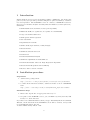
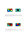
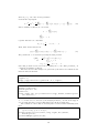
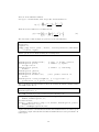
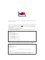
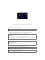
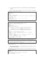
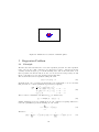
Figure 1: Illustration of the nonlinear Gaussian SVM using different kernel parameters: kerneloption = 0.3 (on the left) and kerneloption = 0.8 (on the right) on
’checkers’ data set. (other parameters: n = 500; sigma=1.4; lambda = 1e-7; C =
1000; kernel=’gaussian’)
xtest1 = reshape ( xtesta1 ,1 , na * nb ) ;
xtest2 = reshape ( xtesta2 ,1 , na * nb ) ;
xtest =[ xtest1 ; xtest2 ] ’;
Figure 1 shows results of nonlinear Gaussian SVM using different kernel parameters.
From the results, you can see: when kernel parameter is larger, the decision
function is more flater. Figure 2 shows results of a nonlinear SVM using different
kernel type to solve the classification task for a classical dataset ’Gaussian’ (with
two gaussianly distributed classes with similar variances but different means).
3.3
Extensions of binary support vector machine
3.3.1
ν-SVM
The ν-SVM has been derived so that the soft margin has to lie in the range of zero
and one.The parameter ν is not controlling the trade off between the training error
and the generalization error; instead it now has two roles:
1. an upper bound on the fraction of margin errors.
2. the lower bound on the fraction of support vectors.
The ν-SVM formulation is as follows:
Pn
min 21 kwk2 − νρ + n1 i=1 ξi
s.t. yi (hw, φ(xi )i + b) ≥ ρ − ξi i = 1, · · · , n
(7)
ξi ≥ 0
i = 1, · · · , n
ρ≥0
ν is a user chosen parameter between 0 and 1.
We consider the Lagrangian:
L=
n
n
n
X
X
1
1X
kwk2 − νρ +
ξi −
αi [yi (hw, φ(xi )i + b) − ρ + ξi ] −
βi ξi − δρ
2
n i=1
i=1
i=1
with
δ ≥ 0,
5
αi ≥ 0,
βi ≥ 0,
i = 1, · · · , n
3
2
2
1
1
0
3
0
1
1
1
0
1
0
−1
−1
−1
0
−1
1
0
−1
−1
−2
0
−1
−1
−1
−2
−3
−3
−2
−1
0
1
2
−3
3
−3
−2
−1
0
1
2
3
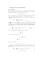
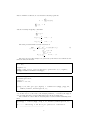
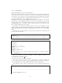
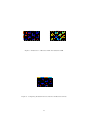
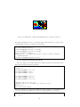
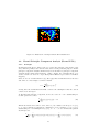
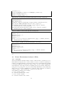
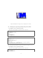
Figure 2: Comparing Gaussian and polynomial Kernels: on the left is final decision function using polynomial kernel(lambda = 1e-10; C = 1; kernel=’poly’;
kerneloption=1;): on the right is final decision function using Gaussian kernel(kernel=’gaussian’; kerneloption=0.25;)
SVM Classification w/o initialisation
SVM Classification with initialisation
2
2
−1
1
1
10
−1
1
0
01
−1
1
0
0
1
−1
1
10
0
−1
1
01
−1
0
0
1
−1
−1
1
0
−1
0
1
−1
−1 −10
0
−1
1
−1
0
1
−1
−1
0 0
−1
0
−1
−10
1
0
−1
1
−3
10
−2
0
−2
−10
1
1
−1 0
3
1
0 −
3
−3
−2
−1
0
1
2
−3
3
−3
−2
10
−1
0
1
2
3
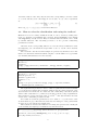
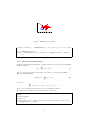
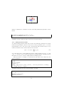
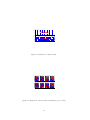
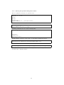
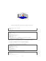
Figure 3: Comparing SVM learning with initialization of Lagrangian Multipliers
(on the right) and without initialization (on the left)
Figure 3 shows that with initialization of Lagrangian Multipliers you can obtain
more flatter decision function.
6
Based on KKT conditions, we obtained the following equations:
w
=
n
X
αi yi φ(xi )
i=1
n
X
αi yi
=
0
i=1
and the following inequality constraints
n
X
αi ≥ ν
i=1
1
,
n
1
0 ≤ βi ≤ ,
n
0 ≤ αi ≤
i = 1, · · · , n
i = 1, · · · , n
The dual problem which is solved is derived as:
Pn Pn
1
min
i=1
j=1 αi αj yi yj k(xi , xj )
2
αi ,i=1,··· ,n
Pn
s.t.
αi yi = 0
Pi=1
n
i=1 αi = ν
0 ≤ αi ≤
1
n,
(8)
∀i = 1, · · · , n.
The data used for this example are generated by the lines below which use the
function function dataset.
n = 100;
sigma =0.4;
[ Xapp , yapp , xtest , ytest ]= dataset ( ’ gaussian ’ ,n ,0 , sigma ) ;
[ Xapp ]= normalizemeanstd ( Xapp ) ;
The decision function is learned +via this segment of code lines:
kernel = ’ gaussian ’;
kerneloption =4;
nu =0.1;
lambda = 1e -12;
[ xsup ,w , w0 , rho , pos , tps , alpha ] = svmnuclass ( Xapp , yapp , nu ,
lambda , kernel , kerneloption ,1) ;
Here the ν parameter was set to 0.1. The function returns the paameters wi =
αi yi in the vector w, the bias b, the margin parameter ρ as well as the support
vectors xsup and their corresponding indexes pos in the training data.
The evaluation of the solution on testing data is achieved when launching these
lines
ypredapp = svmval ( Xapp , xsup ,w , w0 , kernel , kerneloption ,1) ;
% ------- Building a 2 D Grid for function evaluation
------------------------7
3
0
2
0
1
0
0
0
0
0
−1
−3
0
−2
−3
−2
−1
0
1
2
3
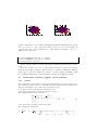
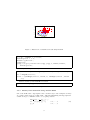
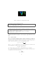
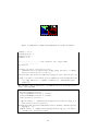
Figure 4: Illustration of ν-SVM
[ xtest1 xtest2 ] = meshgrid ([ -1:.05:1]*3.5 ,[ -1:0.05:1]*3)
;
nn = length ( xtest1 ) ;
Xtest = [ reshape ( xtest1 , nn * nn ,1) reshape ( xtest2 , nn * nn
,1) ];
Figure 4 shows results of ν-SVM to classify the ’Gaussian’ dataset.
3.3.2
Linear Programming SVM
Compared with standard SVM, the decision function in the linear programming
SVM is as follows:
n
X
f (x) =
αi κ(x, xi ) + b
(9)
i=1
where αi take on real values. The kernel κ need not be positive semi-definite.
We consider minimizing:
min L(α, ξ) =
n
X
(|αi | + Cξi )
(10)
i=1
Subject to:
n
X
αi κ(xj , xi ) + b ≥ (1 − ξi ), f orj = 1, · · · , n
i=1
where ξi are positive slack variables and C is a margin parameter.
The data for the example was generated by the codes below:
nbapp =100;
nn =20;
nbtest = nn * nn ;
sigma =0.5;
[ xapp , yapp , xtest , ytest , xtest1 , xtest2 ]= dataset ( ’ gaussian ’ ,
nbapp , nbtest , sigma ) ;
Learning parameters are obtained via the follows lines:
8
2
1.5
1
0.5
1
0
1
−1 0
0
−0.5
−1
−1
−1
0
−1.5
1
−2
−2
−1.5
−1
−0.5
0
0.5
1
1.5
2
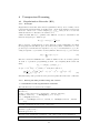
Figure 5: Illustration of Classification task using LPSVM
C = 20; lambda = 0.000001;
kerneloption = 0.5;
kernel = ’ gaussian ’;
verbose =1;
[ xsup ,w ,b , pos ]= LPsvmclass ( xapp , yapp ,C , lambda , kernel ,
kerneloption ) ;
Testing data are generated by:
[ xtest1 xtest2 ] = meshgrid ([ -1:.05:1]*3.5 ,[ -1:0.05:1]*3)
;
nn = length ( xtest1 ) ;
xtest = [ reshape ( xtest1 , nn * nn ,1) reshape ( xtest2 , nn * nn
,1) ];
Predicted value by this LPSVM is obtained:
ypred = reshape ( ypred , nn , nn ) ;
Figure 5 shows result of the example.
3.3.3
Density level estimation using oneclass SVM
One class SVM seeks a hypersphere that contains target class examples as many
as possible while keeps its radius small. Through minimizing this hypersphere’s
volume we hope to minimize chance of accepting outliers.
Pn
1
min 21 kwk2 + νn
i=1 ξi − ρ
s.t. hw, φ(xi )i ≥ ρ − ξi
i = 1, · · · , n
(11)
ξi ≥ 0
i = 1, · · · , n
9
where 0 ≤ ν ≤ 1 is a user chosen parameter.
Consider the Lagrangian:
L=
n
n
n
X
X
1
1 X
kwk2 +
ξi − ρ −
αi [hw, φ(xi )i − ρ − ξi ] −
γi ξi
2
νn i=1
i=1
i=1
(12)
Based on KKT conditions, we can obtain:
w
=
n
X
αi φ(xi )
i=1
n
X
αi
=
1
i=1
together with the box constraints
0 ≤ αi ≤
1
,
νn
∀ i = 1, · · · , n
Then, final decision function is:
f (x) =
n
X
αi hφ(xi ), φ(x)i − ρ =
i=1
n
X
αi k(xi , x) − ρ
(13)
i=1
The parameters αi are derived by solving the dual problem
Pn Pn
1
min
i=1
j=1 αi αj k(xi , xj )
2
α1 ,··· ,αn
Pn
s.t.
i=1 αi = 1
0 ≤ αi ≤
1
νn ,
∀ i = 1, · · · , n
Once this problem is solved for some ν yielding the αi , the offset parameter ρ is
computed from KKT conditions.
The data used for this example are generated by the lines below which use the
function function dataset.
n =100;
sigma =0.2;
[ xapp , yapp ]= dataset ( ’ gaussian ’ ,n ,0 , sigma ) ;
The decision function is learned +via this segment of code lines:
nu =0.1;
kernel = ’ gaussian ’;
kerneloption =0.33;
verbose =1;
[ xsup , alpha , rho , pos ]= svmoneclass ( xapp , kernel , kerneloption
, nu , verbose ) ;
Here the ν parameter was set to 0.1. The function returns the parameters
wi = αi in the vector w, the bias b, the margin parameter ρ as well as the support
vectors xsup and their corresponding indexes pos in the training data.
The evaluation of the solution on testing data is achieved when launching these
lines
[ xtest , xtest1 , xtest2 , nn ]= DataGrid2D
([ -3:0.2:3] ,[ -3:0.2:3]) ;
ypred = svmoneclassval ( xtest , xsup , alpha , rho , kernel ,
kerneloption ) ;
ypred = reshape ( ypred , nn , nn ) ;
10
3.3.4
svmclassnpa
Main ROUTINE For Nearest Point Algorithm.
The basic problem treated by svmclassnpa is one that does not allow classification
violations. The problem is converted to a problem of computing the nearest point
between two convex polytopes. For problems which require classification violations
to be allowed, the violations are quadratically penalized and they are converted into
problems in which there are no classification violations.
This function solve the SVM Classifier problem by transforming the soft-margin
problem into a hard margin problem. The problem is equivalent to look for the
nearest points of two convex hulls. This is solved by the point of minimum norm is
the Minkowski set (U − V ) where U is the class 1 set and V is the class 2 set. For
more detailed information, please find:
S. S. Keerthi, S. K. Shevade, C. Bhattacharyya, and K. R. K. Murthy. A Fast
Iterative Nearest Point Algorithm for Support Vector Machine Classifier Design,
IEEE TRANSACTIONS ON NEURAL NETWORKS, VOL. 11, NO. 1, JANUARY
2000
The data used for this example are generated by the lines below which use the
function function dataset.
N =50;
sigma =0.3;
[ xapp , yapp , xtest , ytest ]= dataset ( ’ gaussian ’ ,N ,N , sigma ) ;
The decision function is learned +via this segment of code lines:
c =1 e6 ;
% c1 =10000;
c2 =100;
c1 =10000;
epsilon = .000001;
gamma =[0.2 0.2 100];
gamma1 =0.4;
kernel = ’ gaussian ’;
verbose = 1;
[ xsup1 , w1 , b1 , pos1 ]= svmclassnpa ( xapp , yapp , c1 , kernel , gamma1
, verbose ) ;
Here the parameter c1 was set to 10000, it caused a slightly modification of
kernel using the following equation:
1
κ∗ (xk , xl ) = κ(xk , xl ) + c1
δkl
where δkl is one if k = l and zero otherwise.
Here the ν parameter was set to 0.1. The function returns the parameters
wi = αi in the vector w, the bias b, the margin parameter ρ as well as the support
vectors xsup and their corresponding indexes pos in the training data.
The evaluation of the solution on testing data is achieved when launching these
lines
ypred1 = svmval ( xtest , xsup1 , w1 , b1 , kernel , gamma1 ) ;
%
--------------------------------------------------------na = s q r t ( length ( xtest ) ) ;
11
NPA Classifier Algorithm Quadratic Penalization
2
1.5
1
1
1
0.5
1
0
−1
0
x2
0
1
1
−0.5
0
−1
−1
−1
0
0
−1.5
−2
−2
−1.5
−1
−0.5
0
x1
0.5
1
1.5
2
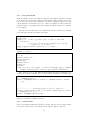
Figure 6: Illustration of SVM for Nearest Point Algorithm with Quadratic Penalization
ypredmat1 = reshape ( ypred1 , na , na ) ;
xtesta1 = reshape ( xtest (: ,1) ,na , na ) ;
Figure 6 shows results of SVM using Nearest Point Algorithm to classify the
’Gaussian’ dataset. The green line denotes the decision function.
3.3.5
Semiparametric SVM
A common semipqrametric method is to fit the data with the parametric model and
train the nonparametric add-on on the errors of the parametric part, i.e. fit the
nonparametric part to the errors. One can show that this is useful only in a very
restricted situation. The decision function is as follows:
f (x) = hw, φ(x)i +
m
X
βi φi (x)
(14)
i=1
Note that this is not so much different from the original setting if we set n = 1 and
φ1 (.) = 1. In the toolbox, if the span matrix for semiparametric learning is given,
the function svmclass can solve semiparametric SVM problem.
The data used for example are generated by the lines below which use the
function dataset.
nbapp =500;
nn =20;
nbtest = nn * nn ;
sigma =0.1;
[ xapp , yapp , xtest , ytest , xtest1 , xtest2 ]= dataset ( ’ CosExp ’ ,
nbapp , nbtest , sigma ) ;
Learning parameters are set by the following code lines:
lambda = 1e -7;
C = 100;
kernel = ’ gaussian ’;
kerneloption =1;
12
0
0
−1
−1
0
1
0.8
0.6
−1
1
1
0.4
0
0
−1
−1
−1
0
0.2
0
1
−1
1
−0.2
0
1
−0.4
0
−1
0
−0.6
1
−0.8
1
1
−1
0
0.5
1
1.5
2
2.5
3
3.5
4
4.5
5
Figure 7: Illustration of Semiparametric SVM
Span matrix is set when launching these lines:
phi = phispan ( xapp , ’ sin2D ’) ;
phitest = phispan ( xtest , ’ sin2D ’) ;
Here, we set the type of parametric functions as ’sin2D’.
Finally, the decision function and the evaluation of the method are achieved:
[ xsup ,w , w0 , tps , alpha ] = svmclass ( xapp , yapp ,C , lambda ,
kernel , kerneloption ,1 , phi ) ;
[ ypred , y1 , y2 ] = svmval ( xtest , xsup ,w , w0 , kernel ,
kerneloption , phitest ,1) ;
Figure 7 shows results of semiparatric SVM to classify the data set ’CosExp’ (established by the function sign(0.95 ∗ cos(0.5 ∗ (exp(x) − 1)))) which is not a easy
task.
3.3.6
Wavelet SVM
The goal of the Wavelet SVM is to find the optimal approximtion or classification
in the space spanned by multidimensional wavelets or wavelet kernels. The idea
behind the wavelet analysis is to express or approximate a signal or function by a
family of functions generated by h(x) called the mother wavelet:
x−c
−1/2
ha,c (x) = |a|
h
a
where x, a, c ∈ R. a is a dilation factor, and c is a translation factor. Therefore the
wavelet transform of a function f (x) can be written as:
Wa,c (f ) = hf (x), ha,c (x)i
For a mother kernel, it is necessary to satisfy mentioned above conditions.
For a common multidimensional wavelet function, we can write it as the product of
one-dimensional (1-D) wavelet functions:
h(x) =
N
Y
i=1
13
h(xi )
where N is the dimension number.
Let h(x) be a mother kernel, then dot-product wavelet kernels are:
!
0
0
N
Y
0
xi − ci
xi − ci
κ(x, x ) =
h
h
a
a
i=1
Then the decision function for classification is:


!
n
N
j
j
X
Y
x
−
x
i
f (x) = sgn 
αi yi
+ b
h
a
i
i=1
j=1
(15)
The data used for this example are generate by the following lines:
n = 160;
ntest =400;
sigma =1.2;
[ Xapp , yapp , xtest , ytest , xtest1 , xtest2 ]= dataset ( ’ Checkers
’ ,n , ntest , sigma ) ;
Kernel options are set when lanching the following lines:
kernel = ’ tensorwavkernel ’;
kerneloption . wname = ’ Haar ’;
% Type of mother wavelet
kerneloption . pow =8;
% number of dyadic
decomposition
kerneloption . par =4;
% number of vanishing
moments
kerneloption . jmax =2;
kerneloption . jmin = -2;
kerneloption . father = ’ on ’;
% use father wavelet in
kernel
kerneloption . coeffj =1/ s q r t (2) ; % coefficients of
ponderation of a given j scale
Here q 2D Tensor-Product Kernel are used. To evaluate the Wavelet SVM, a Gaussian SVM is introduced:
kernel2 = ’ gaussian ’;
kernel2option =0.5;
The SVM calculation process is achieved by the following code:
[ xsup ,w , w0 , tps , alpha ] = svmclass ( Xapp , yapp ,C , lambda ,
kernel , kerneloption ,1) ;
tpstensor = toc ;
ypred = svmval ( Xtest , xsup ,w , w0 , kernel , kerneloption ,[ ones (
length ( Xtest ) ,1) ]) ;
ypred = reshape ( ypred , nn , nn ) ;
Figure 8 shows that: both the Wavelet kernel and Gaussian kernel can achieve good
performance, figure 9 shows that the Wavelet SVM achieves better performance in
some region.
14
2
2D Tensor−Product Kernel
0
Gaussian Kernel
2
0
0
0
1.5
1.5
1
0
0
0
0
0
0
0
0
0
0
1
0.5
0
0.5
0
0
0
0
0
0
0
0
0
−0.5
0
−1
0
0
0
−0.5
0
0
−1
0
0
0
0
0
0
−1.5
−1.5
0
0
0
0
0
−2
−2
−1.5
−1
−0.5
0
0.5
1
1.5
−2
−2
2
−1.5
−1
−0.5
0
0.5
1
1.5
2
Figure 8: Illustration of Wavelet SVM and Gaussian SVM
Comparing Gaussian Kernel Solution and Haar Kernels
0
0
2
1.5
0
0
0
1
0
0
0.5
0
0
0
0
0
0
−0.5
−1
0
0
0
0
−2
−2
0
0
−1.5
−1.5
−1
−0.5
0
0.5
1
1.5
2
Figure 9: Comparing Gaussian kernel solutions and Wavelet kernels
15
3.3.7
Large Scale SVM
SVM algorithm for large scale using decomposition algorithm. The whole training
set is divided into many subset which is much smaller. When training, remove the
non support vectors from the working set and fill the chunk up with the data the
current estimator would make errors on to form new working set. Then retrain the
system and keep on iterating until after training the KKT-conditions are satisfied
for all samples.
The data used for this large scale classification task are generated by the lines
below which use the function function dataset.
n = 7000;
nbtest =1600;
sigma =0.3; % This problem needs around a thousand
iteration
% you can speed up the example by setting
sigma =0.3 for instance
[ Xapp , yapp ]= dataset ( ’ gaussian ’ ,n ,0 , sigma ) ;
Here the size of training set is 7000. The decision function is learned +via this
segment of code lines:
lambda = 1e -10;
C = 10;
kernel = ’ gaussian ’;
kerneloption =1;
qpsize =300;
chunksize =300;
verbose =1;
span =[];
[ xsup ,w , w0 , pos , tps , alpha ] = svmclassLS ( Xapp , yapp ,C , lambda
, kernel , kerneloption , verbose , span , qpsize , chunksize ) ;
The chunksize is set to 300, which is much smaller than that of working set. To
evaluate the solution on testing data is achieved when lanching the following lines.
[ xtest1 xtest2 ] = meshgrid ( l i n s p a c e ( -4 ,4 , s q r t ( nbtest ) ) ) ;
nn = length ( xtest1 ) ;
Xtest = [ reshape ( xtest1 , nn * nn ,1) reshape ( xtest2 , nn * nn
,1) ];
% - - - - - - - - - - - - - - Evaluating the decision function
ypred = svmval ( Xtest , xsup ,w , w0 , kernel , kerneloption ,[ ones (
length ( Xtest ) ,1) ]) ;
ypred = reshape ( ypred , nn , nn ) ;
Figure 10 shows results of SVM algorithm for large scale using decomposition
method to classify the ’Gaussian’ dataset.
3.3.8
svmclassL2LS
Large scale SVM algorithm with quadratic penalty. The data used for this example
are generated by the lines below which use the function function dataset.
16
4
3
0
1
2
1
0
0
1
−1
−1
0
1
1
−1
0
0
−1
−1
−2
−1
−3
−4
−4
−3
−2
−1
0
1
2
3
4
Figure 10: Illustration of SVM algorithm for large scale using decomposition method
n = 500;
sigma =0.3;
[ Xapp , yapp , xtest , ytest ]= dataset ( ’ gaussian ’ ,n ,0 , sigma ) ;
The decision function is learned +via this segment of code lines:
lambda = 1e -12;
C = 1;
kernel = ’ poly ’;
kerneloption =2;
qpsize =10;
verbose =1;
span =1;
[ xsup ,w , w0 , pos , tps , alpha ] = svmclassL2LS ( Xapp , yapp ,C ,
lambda , kernel , kerneloption , verbose , span , qpsize ) ;
[ xsup1 , w1 , w01 , pos1 , tps , alpha1 ] = svmclassL2 ( Xapp , yapp ,C ,
lambda , kernel , kerneloption , verbose , span ) ;
The following lines are introduced to evaluate the decision function:
ypred = svmval ( Xtest , xsup ,w , w0 , kernel , kerneloption ,[ ones (
length ( Xtest ) ,1) ]) ;
ypred = reshape ( ypred , nn , nn ) ;
ypred1 = svmval ( Xtest , xsup1 , w1 , w01 , kernel , kerneloption ,[
ones ( length ( Xtest ) ,1) ]) ;
ypred1 = reshape ( ypred1 , nn , nn ) ;
Figure fig:exsvmlsl2 shows results of SVM algorithm with quadratic penalization.
3.3.9
Multi-class SVM
One against All (OAA) algorithm and One Against One (OAO) are popular algorithms to solve multi-classification task. OAA SVM required unanimity among all
SVM: a data point would be classified under a certain class if and only if that class’s
SVM accepted it and all other classes’ SVMs rejected it, and OAO SVM approach
17
3
2
1
1
1
0
0
0
−1
1
−1
0
−1
1
−1
−2
−1
−3
−2
−1
0
1
2
0
−3
3
Figure 11: Illustration of SVM algorithm using decomposition method with
quadratic penalization
trains a binary SVM for anytwo classes of data and obtains a decision function.
decision functions. A voting strategy
Thus, for a k-class problem, there are k(k−1)
2
is used where the testing point is designated to be in a class with the maximum
number of votes.
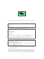
1. One Against All multi-class SVM
The data used for a multi-classification task are generated by the lines below which
use the function function dataset.
n =20;
sigma =1;
x1 = sigma *randn(1 , n ) -1.4;
x2 = sigma *randn(1 , n ) +0;
x3 = sigma *randn(1 , n ) +2;
y1 = sigma *randn(1 , n ) -1.4;
y2 = sigma *randn(1 , n ) +2;
y3 = sigma *randn(1 , n ) -1.4;
xapp =[ x1 x2 x3 ; y1 y2 y3 ] ’;
yapp =[1* ones (1 , n ) 2* ones (1 , n ) 3* ones (1 , n ) ] ’;
Here the training set contains three different classes and there are 20 samples in
each class. The decision function is learned +via this segment of code lines:
c = 1000;
lambda = 1e -7;
kerneloption = 2;
kernel = ’ gaussian ’;
verbose = 1;
% - - - - - - - - - - - - - - - - - - - - - One Against All algorithms
---------------nbclass =3;
[ xsup ,w ,b , nbsv ]= s v m m u l t i c l a s s o n e a g a i n s t a l l ( xapp , yapp ,
nbclass ,c , lambda , kernel , kerneloption , verbose ) ;
18
4
classe 1
classe 2
classe 3
Support Vector
3
2
1
0
−1
−2
−3
−4
−4
−3
−2
−1
0
1
2
3
4
Figure 12: Illustration of multi-class SVM using one against all method
The OAL algorithm is used to obtain the final decision function. Codes in the
following lines are used to evaluate its performence.
[ xtesta1 , xtesta2 ]= meshgrid ([ -4:0.1:4] ,[ -4:0.1:4]) ;
[ na , nb ]= s i z e ( xtesta1 ) ;
xtest1 = reshape ( xtesta1 ,1 , na * nb ) ;
xtest2 = reshape ( xtesta2 ,1 , na * nb ) ;
xtest =[ xtest1 ; xtest2 ] ’;
[ ypred , maxi ] = svmmultival ( xtest , xsup ,w ,b , nbsv , kernel ,
kerneloption ) ;
ypredmat = reshape ( ypred , na , nb ) ;
2. One Against One multi-class SVM
The data using for the multi-classification task are generated by the lines below
which use the function function dataset.
n =100;
sigma =0.5;
x1 = sigma *randn(1 , n ) -1.4;
x2 = sigma *randn(1 , n ) +0;
x3 = sigma *randn(1 , n ) +2;
y1 = sigma *randn(1 , n ) -1.4;
y2 = sigma *randn(1 , n ) +2;
y3 = sigma *randn(1 , n ) -1.4;
xapp =[ x1 x2 x3 ; y1 y2 y3 ] ’;
yapp =[1* ones (1 , n ) 2* ones (1 , n ) 3* ones (1 , n ) ] ’;
nbclass =3;
[ n1 , n2 ]= s i z e ( xapp ) ;
Here the training set contains three different classes and there are 100 samples in
each class. The decision function is learned +via this segment of code lines:
%
Learning and Learning Parameters
c = 1000;
19
4
classe 1
classe 2
classe 3
Support Vector
3
2
1
0
−1
−2
−3
−4
−4
−3
−2
−1
0
1
2
3
4
Figure 13: Illustration of multi-class SVM using one against one method
lambda = 1e -7;
kerneloption = 1;
kernel = ’ poly ’;
verbose = 0;
% - - - - - - - - - - - - - - - - - - - - - One Against One algorithms
---------------nbclass =3;
%
% [ xsup ,w ,b , nbsv , classifier , pos ]=
s v m m u l t i c l a s s o n e a g a i n s t o n e ( xapp , yapp , nbclass ,c , lambda ,
kernel , kerneloption , verbose ) ;
% kerneloptionm . matrix = svmkernel ( xapp , kernel , kerneloption )
;
[ xsup ,w ,b , nbsv , classifier , pos ]= s v m m u l t i c l a s s o n e a g a i n s t o n e
([] , yapp , nbclass ,c , lambda , ’ numerical ’ , kerneloptionm ,
verbose ) ;
The following codes are introduced to establish the test data and evaluate performance of the algorithm
[ xtesta1 , xtesta2 ]= meshgrid ([ -4:0.1:4] ,[ -4:0.1:4]) ;
[ na , nb ]= s i z e ( xtesta1 ) ;
xtest1 = reshape ( xtesta1 ,1 , na * nb ) ;
xtest2 = reshape ( xtesta2 ,1 , na * nb ) ;
xtest =[ xtest1 ; xtest2 ] ’;
% [ ypred , maxi ] = s v m m u l t i v a l o n e a g a i n s t o n e ( xtest , xsup ,w ,b ,
nbsv , kernel , kerneloption ) ;
kerneloptionm . matrix = svmkernel ( xtest , kernel , kerneloption ,
xapp ( pos ,:) ) ;
[ ypred , maxi ] = s v m m u l t i v a l o n e a g a i n s t o n e ([] ,[] , w ,b , nbsv , ’
numerical ’ , kerneloptionm ) ;
20
4
4.1
4.1.1
Unsupervised Learning
Regularization Networks (RN)
Principle
Regularization Networks derived from regularization theory. It is a family of feedforward neural networks with one hidden layer. ’Learn from examples’ is its typical
n
character. Given a set of data samples {(xi , yi )}i=1 Our goal is to recover the
unknown function or find the best estimate of it.
Unlike in SVM, RN try to optimize some different smoothness criterium for the
function in input space. Thus we get
Rreg [f ] := Remp [f ] +
λ
kP f k2
2
(16)
Here P denotes a regularization operator which is positive semidefinite It realizes
the mapping from the Hilbert space H of functions f under consideration to a dot
product space D such that the expression < P f.P g > is well defined for f, g ∈ H.
Using an expansio of f in terms of some symmetric function κ(xi , xj ), we achieves:
f (x) =
n
X
αi κ(xi , x) + b
(17)
i=1
Here the κ needs not fulfill Mercer’s condition. Similar to the one for SVs, equation
16 leads to a quadratic programming problem. By computing Wolfe’s dual and
using
Dij :=< (P k)(xi , .).(P k)(xj , .) >
we get α = D−1 K(β − β ∗ ) with β, β ∗ being the solution of
Pn
1
∗
T
−1
K(β ∗ − β) − (β ∗ − β)T y − i=1 (βi + βi∗ )
minP
2 (β − β) KD
n
s.t. i=1 (βi − βi∗ ) = 0
(18)
But this setting of the problem does not preserve sparsity in terms of the coefficients.
4.1.2
Solving the RN problem using the toolbox
1. Classification with regularization networks
The Checker Data are used for the example:
nbapp =600;
nbtest =0;
[ xapp , yapp ]= dataset ( ’ Checkers ’ , nbapp , nbtest ) ;
[ xtest1 xtest2 ] = meshgrid ([ -2:0.1:2]) ;
nn = length ( xtest1 ) ;
xtest = [ reshape ( xtest1 , nn * nn ,1) reshape ( xtest2 , nn * nn
,1) ];
Learning parameters are set by the codes below:
lambda = 1;
kernel = ’ gaussian ’;
kerneloption =0.2;
The line below returns the parameters c and d that equation 16 is minimized.
[c , d ]= rncalc ( xapp , yapp , kernel , kerneloption , lambda ) ;
21
Regularization Networks for CheckerBoard Classification
2
0
0
1.5
1
0
0
0
0
0
0.5
0
0
0
0
0
−0.5
0
0
0
0
−1
0
0
−1.5
−2
−2
−1.5
−1
−0.5
0
0.5
1
1.5
2
Figure 14: Illustration of RN for CheckerBoard Classifiation
Then we can obtain the output of RN:
ypred = rnval ( xapp , xtest , kernel , kerneloption ,c , d ) ;
Figure 14 shows results of Regulation Networks for CheckerBoard Classification.
2. Semiparametric classification with regularization networks
Training set and testing set are generated by the codes below:
nbapp =300;
nbtest =25;
[ xapp , yapp ]= dataset ( ’ CosExp ’ , nbapp , nbtest ) ;
[ xtest1 xtest2 ] = meshgrid ( l i n s p a c e (0 ,4 , nbtest ) , l i n s p a c e
( -1 ,1 , nbtest ) ) ;
Learning parameters are set via the following line:
lambda = 1;
kernel = ’ gaussian ’;
kerneloption =0.1;
T = phispan ( xapp , ’ sin2d ’) ;
For semiparametric learning, the span matrix Tij = φj (xi ) is given in form of T .
Then we get the parameters c and d through the line below:
[c , d ]= rncalc ( xapp , yapp , kernel , kerneloption , lambda , T ) ;
Finally, the predict value of RN is obtained:
ypred = rnval ( xapp , xtest , kernel , kerneloption ,c ,d , T ) ;
ypred = reshape ( ypred , nn , nn ) ;
Figure 15 shows results of semiparametric RN classification in CosExp dataset.
22
SemiParametric Regularization Networks Classification
0
1
0.8
0.6
0
0
0.4
0
0.2
0
0
0
−0.2
0
0
−0.4
−0.6
0
−0.8
0
−1
0
0.5
1
1.5
2
2.5
3
3.5
4
Figure 15: Illustration of Semiparametric RN Classification
4.2
4.2.1
Kernel Principle Component Analysis (Kernel PCA)
Principle
Standard PCA is used to find a new set of axes (the principle components of the
data) which hopefully better describes the data for some particular purpose. Kernel
principal component analysis (kernel PCA) is an extension of principal component
analysis (PCA) using kernel methods. Using a kernel, the originally linear operations of PCA are done in a reproducing kernel Hilbert space with a non-linear
mapping.
First, we choose a transformation φ(x), We apply these transformations to the data
and arrive at a new sample covariance matrix:
n
C=
1X
φ(xi )φ(xi )T
n i=1
(19)
Noting that the transformations must conserve the assumption that the data is
centered over the rigion.
To find the first principle component, we need to solve λν = CV . Substituting for
C, this equation becomes:
n
1X
(φ(xi )(φT (xi )ν) = λν
n i=1
(20)
This is the function we want to solve, Since λ 6= 0, ν must be in the spac
P of φ(xi ),
i.e. ν can be written by some linear combination of φ(xi ), namely, ν = i αi φ(xi ).
Substituting for ν and multiplied by φ(xk ), k = 1, · · · , n at both sides of equation
20, this give us:
n
n
X
1X X T
αj
(φ (xk )φ(xi ))(φT (xi )φ(xj )) = λ
αi φT (xk )φ(xi )
n j
i=1
i=1
23
(21)
Define the Gram Matrix
Kij = K(xi , xj ) = φT (xi )φ(xj )
Using the define of κ, we can rewrite the equation 20 as:
λκα =
1 2
K α
n
(22)
Then we have to solve an eigenvalue problem on the Gram matrix. Now to extract
a principle component we simply take
yi = ν t x
For all i, where ν is the eigenvector corresponding to that principle component,
noting that
X
X
yi =
αi (φT (xj )φ(xi )) =
αj K(xi , xj )
(23)
j
4.2.2
j
Solving the problem using the toolbox
We utilize 3 examples to make the description more detail.
1. Example of Kernel PCA on artificial data
We use the following lines to establish the training set and testing set for the
example:
x1 =0.2* randn (100 ,1) +0.5;
x2 = x1 +0.2* randn (100 ,1) +0.2;
x =[ x1 x2 ];
y1 =1* randn (100 ,1) +0.5;
y2 = - y1 .^2+0.05* randn (100 ,1) +0.2;
y =[ y1 y2 ];
xpca =[ x ; y ];
xpca =randn (100 ,2) *[0.2 0.001; 0.001 0.05];
vect =[ -1:0.05:1];
nv = length ( vect ) ;
[ auxx , auxy ]= meshgrid ( vect ) ;
xtest =[ reshape ( auxx , nv * nv ,1) reshape ( auxy , nv * nv ,1) ];
The eigenvalue and eigenvector are learned via this segment of code lines:
kernel = ’ poly ’;
kerneloption =1;
max_eigvec =8;
[ eigvect , eigval ]= kernelpca ( xpca , kernel , kerneloption ) ;
max_eigvec =min([ length ( eigval ) max_eigvec ]) ;
feature = kernelpcaproj ( xpca , xtest , eigvect , kernel ,
kerneloption ,1: max_eigvec ) ;
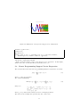
Figure 16 shows results of Kernel PCA: Data and IsoValues on the different eigenvectors.
24
−1
−1
−0.8
−0.6
−0.4
1 Eigenvalue=0.003
−7.5672
0.5
−5.05867
−2.55014
0
−0.0416113
2.46692
−0.5
4.97545
7.48398
−1
−1
−0.8
−0.6
−0.4
0.2
0.4
−7.5672
−5.05867
−2.55014
−0.0416113
2.46692
4.97545
7.48398
−0.2
0
7.59247
0
5.08394
−0.2
2.57541
0.0668822
−4.95018
−7.45871
0
−0.5
−2.44165
1 Eigenvalue=0.042
0.5
0.6
0.8
1
−7.5672
−5.05867
−2.55014
−0.0416113
2.46692
4.97545
7.48398
0.2
0.4
0.6
0.8
1
Figure 16: Illustration of Kernel PCA
1.5
Eigenvalue=0.251
Eigenvalue=0.233
Eigenvalue=0.052
Eigenvalue=0.044
1.5
1.5
1.5
1
1
1
1
0.5
0.5
0.5
0.5
0
0
−0.5
−1
1.5
0
1
−0.5
−1
0
0
1
−0.5
−1
0
0
1
−0.5
−1
0
1
Eigenvalue=0.037
Eigenvalue=0.033
Eigenvalue=0.031
Eigenvalue=0.025
1.5
1.5
1.5
1
1
1
1
0.5
0.5
0.5
0.5
0
−0.5
−1
0
0
1
−0.5
−1
0
0
1
−0.5
−1
0
0
1
−0.5
−1
0
1
Figure 17: Illustration of Kernel PCA and Kernelpcaproj routine
25
2. A toy example that make use of Kernel PCA and Kernelpcaproj
routine
The data set used in this example is composed of three clusters. Parameters
that used to generate the data set is set:
rbf_var = 0.1;
xnum = 4;
ynum = 2;
max_ev = xnum * ynum ;
% ( extract features from the first < max_ev > Eigenvectors )
x_test_num = 15;
y_test_num = 15;
cluster_pos = [ -0.5 -0.2; 0 0.6; 0.5 0];
cluster_size = 30;
The training set and testing set are generated via the codes below:
num_clusters = s i z e ( cluster_pos ,1) ;
train_num = num_clusters * cluster_size ;
patterns = z e r o s ( train_num , 2) ;
range = 1;
randn( ’ seed ’ , 0) ;
f o r i =1: num_clusters ,
patterns (( i -1) * cluster_size +1: i * cluster_size ,1) =
cluster_pos (i ,1) +0.1* randn( cluster_size ,1) ;
patterns (( i -1) * cluster_size +1: i * cluster_size ,2) =
cluster_pos (i ,2) +0.1* randn( cluster_size ,1) ;
end
test_num = x_test_num * y_test_num ;
x_range = - range :(2* range /( x_test_num - 1) ) : range ;
y_offset = 0.5;
y_range = - range + y_offset :(2* range /( y_test_num - 1) ) :
range + y_offset ;
[ xs , ys ] = meshgrid ( x_range , y_range ) ;
test_patterns (: , 1) = xs (:) ;
test_patterns (: , 2) = ys (:) ;
Then Kernel PCA and Kernelpcaroj are introduced to deal with the problem:
[ evecs , evals ]= kernelpca ( patterns , kernel , kerneloption ) ;
test_features = kernelpcaproj ( patterns , test_patterns , evecs ,
kernel , kerneloption ,1: max_ev ) ;
Figure 17 shows results of a toy example that make use of Kernel PCA and Kernelpcaproj routine.
3. Example of kernel PCA as prepocessing stage for a linear (or nonlinear) SVM classifier
This method is also called multilayers SVM. The data for this example are generated
by the following codes:
N =200;
sigma =1;
[ xapp yapp ]= dataset ( ’ clowns ’ ,N ,N , sigma ) ;
[x , y ]= meshgrid ( -4:0.1:4) ;
26
nx = s i z e (x ,1) ;
xtest =[ reshape (x , nx * nx ,1) reshape (y , nx * nx ,1) ];
indplus = f i n d ( yapp ==1) ;
indmoins = f i n d ( yapp == -1) ;
Then the data are pre-treated by Kernel PCA method via the codes below:
kernel = ’ gaussian ’;
kerneloption =1;
max_eigvec =500;
[ eigvect , eigval ]= kernelpca ( xapp , kernel , kerneloption ) ;
max_eigvec =min([ length ( eigval ) max_eigvec ]) ;
appfeature = kernelpcaproj ( xapp , xapp , eigvect , kernel ,
kerneloption ,1: max_eigvec ) ;
testfeature = kernelpcaproj ( xapp , xtest , eigvect , kernel ,
kerneloption ,1: max_eigvec ) ;
A linear classifier is achieved through the following lines:
c = 1000;
lambda =1 e -7;
kerneloption = 1;
kernel = ’ poly ’;
verbose = 0;
[ xsup ,w ,b , pos ]= svmclass ( appfeature , yapp ,c , lambda , kernel ,
kerneloption , verbose ) ;
And a nonlinear classifier is achieved through the codes below:
c = 1000;
lambda =1 e -7;
kerneloption = 1;
kernel = ’ gaussian ’;
verbose = 0;
[ xsup ,w ,b , pos ]= svmclass ( xapp , yapp ,c , lambda , kernel ,
kerneloption , verbose ) ;
Figure 18 shows results of the multilayers SVM when classifing the ’clowns’ data
set.
4.3
4.3.1
Linear Discriminant Analysis (LDA)
Principle
Linear Discriminant Analysis (LDA) is used to find the linear combination of features which best separate two or more classes of objects or events. It explicitly attempts to model the difference between the classes of data. LDA explicitly attempts
to model the difference between the classes of data. For two classes classification
task, LDA approaches the problem by assuming that the probability density func−
−
tions p(→
x |y = 1) and p(→
x |y = 0) are both normally distributed. It also makes the
simplifying
homoscedastic
assumption (i.e. that the class covariances are identical,
P
P
P
so y=0 = y=1 = ) and that the covariances have full rank.
Let’s assume m clusters and n samples:
C: total covariance matrix
G: convariance matrix of the centers
C: total covariance matrix
G: convariance matrix of the centers
27
4
KPCA + linear SVM solution
NonLinear SVM
3
2
1
0
−1
−2
−3
−4
−4
−3
−2
−1
0
1
2
3
4
Figure 18: Illustration of Kernel PCA and Kernelpcaproj routine
→
−
v i : ith discriminant axis (i = 1, · · · , m − 1)
LDA maximizes the variance ratio:
λi =
→
−
−
v Ti G→
vi
Interclass variance
→ λi = →
−
→
T
T otal variance
v i C−
vi
(24)
The solution is based on an eigen system:
−
−
λi →
v i = C −1 G→
vi
(25)
The eigen vectors are linear comhinations of the learning samples:
→
−
vi=
n
X
−
αij →
xj
(26)
i=1
4.4
Solving the LDA problems using the toolbox
4.5
Smallest sphere
4.5.1
Princople
How to find the smallest sphere that would include all data?
Training set is x1 , · · · , xn , seeking the smallest sphere that would include all points
lead to the QP problem:
Pn
Pn
max W (α) = i=1 αi κ(xi , xi ) − i,j=1 αi αj κ(xi , xi )
Pn
(27)
s.t. i=1 αi = 1
αi ≥ 0
i = 1, · · · , n
The radius of the smallest sphere is:
r∗ =
p
W (α∗ )
28
4.5.2
Sloving the problem using the toolbox
The two dimension data here are generated by:
N =2;
xapp =[1 1; 2 2];
N =100;
rho =4;
moy =[0 0];
xapp =randn(N ,2) + ones (N ,1) * moy ;
Then the outliers are abandoned:
mod2 =sum(( xapp - ones (N ,1) * moy ) .^2 ,2) ;
xapp ( f i n d ( mod2 > rho ) ,:) =[];
Learning parameters are set via the following lines:
kernel = ’ poly ’;
C =0.001;
verbose =1;
kerneloption =1;
In this example, we have to take C into account when changing the kernel:
K = svmkernel ( xapp , kernel , kerneloption ) ;
kerneloption . matrix = K +1/ C * eye ( s i z e ( xapp ,1) ) ;
Finally, we get the radius and the center of the sphere when launching the line:
[ beta , r2 , pos ]= r2smallestsphere ([] , kernel , kerneloption ) ;
Figure 19 shows the results of smallest sphere, and you can get the radius is
31.4717 in the command window.
29
8
6
4
2
0
−2
−4
−6
−8
−8
−6
−4
−2
0
2
4
6
8
Figure 19: Illustration of solution of smallest sphere
5
5.1
Regression Problem
Principle
We introduce the loss function to solve the regression problem. In -SV regression
task, out goal is to find a function f (x) that has at most deviation from the
actually obtained targets yi for all the training data, and at the same time, is as
flat as possible. In other words, we do not care about errors as long as they are less
than , but will not accept any deviation larger than this.
The decision function for regression taking the form:
f (x) = hw, φ(x)i + b
(28)
Flatness in the case of equation 28 means that one seeks small w. So we can write
this problem as a convex optimization problem by requiring:
Pn
min 21 kwk2 + C i=1 (ξi + ξi∗ )
s.t. yi − hw, φ(x)i − b ≤ + ξi i = 1, · · · , n
(29)
hw, φ(x)i + b − yi ≤ + ξi∗ i = 1, · · · , n
∗
ξi , ξi ≥ 0
i = 1, · · · , n
The so-called −insensitive loss function |ξi | is described by:
|ξ| := max(0, |yi − f (xi )| − )
(30)
Similar with Support vector classification, we can construct a Lagrange function to
solve the optimization problem. Finally, we can obtain:
w=
n
X
(αi − αi∗ )φ(xi )
(31)
i=1
Therefore:
f (x) =
n
X
(αi − αi∗ ) hφ(xi ), φ(x)i + b =
i=1
n
X
(αi − αi∗ )κ(xi , x) + b
i=1
30
(32)
Support Vector Machine Regression
1
0.8
0.6
0.4
y
0.2
0
−0.2
−0.4
−0.6
−0.8
−1
0
1
2
3
4
x
5
6
7
8
Figure 20: Illustration of Support Vector Regression for 1D data
5.2
Solving the regression problem using the toolbox
1. 1D Support vector regression problem
The data for this example are generated by the codes below:
n =200;
x = l i n s p a c e (0 ,8 , n ) ’;
xx = l i n s p a c e (0 ,8 , n ) ’;
xi = x ;
yi = cos (exp( x ) ) ;
y = cos (exp( xx ) ) ;
Learning parameters are set via the follwing lines:
C = 10; lambda = 0.000001;
epsilon = .1;
kerneloption = 0.01;
kernel = ’ gaussian ’;
verbose =1;
[ xsup , ysup ,w , w0 ] = svmreg ( xi , yi ,C , epsilon , kernel ,
kerneloption , lambda , verbose ) ;
Figure 20 shows results of Support Vector Regression for 1D data, the blue line
denotes the final decision function, and the red points denote support vectors.
2. 2D Support vector regression problem
The data for this example are generated by the codes below:
N =100;
x1 =2* randn(N ,1) ;
x2 =2* randn(N ,1) ;
31
Support Vector Machine Regression
1
0.8
0.6
0.4
0.2
0
4
2
4
2
0
0
−2
y
−2
−4
−4
x
Figure 21: Illustration of Support Vector Regression for 2D data
y =exp( -( x1 .^2+ x2 .^2) *2) ;
x =[ x1 x2 ];
Learning parameters are set via the follwing lines:
C = 1000;
lambda = 1e -7;
epsilon = .05;
kerneloption = 0.30;
kernel = ’ gaussian ’;
verbose =1;
[ xsup , ysup ,w , w0 ] = svmreg (x ,y ,C , epsilon , kernel ,
kerneloption , lambda , verbose ) ;
Figure 21 shows result of Gaussian Support vector regression for 2D data.
3. Large scale Support vector regression problem
The following codes return data for this example:
n =600;
x = l i n s p a c e (0 ,5 , n ) ’;
xx = l i n s p a c e (0 ,5 , n ) ’;
xi = x ;
yi = cos (exp( x ) ) ;
y = cos (exp( xx ) ) ;
Learning parameters are set via the lines below:
C = 10; lambda = 0.000001;
epsilon = .1;
kerneloption = 0.4;
32
Support Vector Machine Regression
1.5
1
y
0.5
0
−0.5
−1
−1.5
0
0.5
1
1.5
2
2.5
x
3
3.5
4
4.5
5
Figure 22: Illustration of Large Scale Support Vector Regression
kernel = ’ gaussian ’;
verbose =1;
qpsize =100;
[ xsup , ysup ,w , w0 ] = svmregls ( xi , yi ,C , epsilon , kernel ,
kerneloption , lambda , verbose , qpsize ) ;
Here the chunking method is adopted to solve the large scale regression problem,
and the size of QP method is 100.
Figure 22 shows results of large scale support vector regression. In this figure,
width of the tube around the final decision function is /2.
5.3
Linear Programming Support Vector Regression
The decision function in the linear programming SVM for regression is as follows:
f (x) =
n
X
αi κ(x, xi ) + b
(33)
i=1
where αi take on real values.
We consider minimizing:
min L(α, ξ) =
n
X
(αi +
i=1
Subject to:
αi∗ )
n
X
+C
(ξi + ξi∗ )
i=1
Pn
∗
i=1 (αi − αi )κ(xj , xi ) − b
∗
i=1 (αi − αi )κ(xj , xi ) + b − yi
αi , αi∗ , ξi , ξi∗ ≥ 0
yP
i−
n
≤ + ξi
≤ + ξi∗
where ξi are positive slack variables and C is a margin parameter.
The data for the example was generated by the codes below:
33
(34)
Linear Programming Support Vector Machine Regression
3.5
3
y
2.5
2
1.5
1
0.5
0
0.5
1
1.5
2
2.5
x
3
3.5
4
4.5
5
Figure 23: Illustration of Linear Programming Support Vector Regression
n =100;
x = l i n s p a c e (0 ,5 , n ) ’;
xx = l i n s p a c e (0 ,5 , n ) ’;
xi = x ;
yi = cos (exp( x ) ) +2;
y = cos (exp( xx ) ) +2;
Learning parameters are set via the lines below:
C = 10; lambda = 0.000001;
epsilon = .1;
kerneloption = 0.1;
kernel = ’ gaussian ’;
verbose =1;
[ xsup , ysup ,w , w0 ] = LPsvmreg ( xi , yi ,C , epsilon , lambda , kernel
, kerneloption , verbose ) ;
Figure 23 shows result of Linear Programming SVM for regression task.Compared
with standard SVM, it has less support vectors.
34