
1
Applied Data Science
Ian Langmore
Daniel Krasner
2
Contents
I
Programming Prerequisites
1 Unix
1.1 History and Culture . . . .
1.2 The Shell . . . . . . . . . .
1.3 Streams . . . . . . . . . . .
1.3.1 Standard streams . .
1.3.2 Pipes . . . . . . . .
1.4 Text . . . . . . . . . . . . .
1.5 Philosophy . . . . . . . . .
1.5.1 In a nutshell . . . .
1.5.2 More nuts and bolts
1.6 End Notes . . . . . . . . . .
1
.
.
.
.
.
.
.
.
.
.
.
.
.
.
.
.
.
.
.
.
.
.
.
.
.
.
.
.
.
.
.
.
.
.
.
.
.
.
.
.
.
.
.
.
.
.
.
.
.
.
.
.
.
.
.
.
.
.
.
.
.
.
.
.
.
.
.
.
.
.
.
.
.
.
.
.
.
.
.
.
2
2
3
5
6
7
9
10
10
10
11
2 Version Control with Git
2.1 Background . . . . . . . . . . . . . . . . . . . . .
2.2 What is Git . . . . . . . . . . . . . . . . . . . . .
2.3 Setting Up . . . . . . . . . . . . . . . . . . . . . .
2.4 Online Materials . . . . . . . . . . . . . . . . . .
2.5 Basic Git Concepts . . . . . . . . . . . . . . . . .
2.6 Common Git Workflows . . . . . . . . . . . . . .
2.6.1 Linear Move from Working to Remote . .
2.6.2 Discarding changes in your working copy
2.6.3 Erasing changes . . . . . . . . . . . . . .
2.6.4 Remotes . . . . . . . . . . . . . . . . . . .
2.6.5 Merge conflicts . . . . . . . . . . . . . . .
.
.
.
.
.
.
.
.
.
.
.
.
.
.
.
.
.
.
.
.
.
.
.
.
.
.
.
.
.
.
.
.
.
.
.
.
.
.
.
.
.
.
.
.
.
.
.
.
.
.
.
.
.
.
.
.
.
.
.
.
.
.
.
.
.
.
.
.
.
.
.
.
.
.
.
.
.
13
13
13
14
14
15
15
16
17
17
17
18
.
.
.
.
.
.
.
.
.
.
.
.
.
.
.
.
.
.
.
.
.
.
.
.
.
.
.
.
.
.
.
.
.
.
.
.
.
.
.
.
.
.
.
.
.
.
.
.
.
.
.
.
.
.
.
.
.
.
.
.
.
.
.
.
.
.
.
.
.
.
.
.
.
.
.
.
.
.
.
.
.
.
.
.
.
.
.
.
.
.
.
.
.
.
.
.
.
.
.
.
.
.
.
.
.
.
.
.
.
.
3 Building a Data Cleaning Pipeline with Python
19
3.1 Simple Shell Scripts . . . . . . . . . . . . . . . . . . . . . . . 19
3.2 Template for a Python CLI Utility . . . . . . . . . . . . . . . 21
i
ii
II
CONTENTS
The Classic Regression Models
23
4 Notation
24
4.1 Notation for Structured Data . . . . . . . . . . . . . . . . . . 24
5 Linear Regression
5.1 Introduction . . . . . . . . . . . . . . . . . . . . . . . . .
5.2 Coefficient Estimation: Bayesian Formulation . . . . . .
5.2.1 Generic setup . . . . . . . . . . . . . . . . . . . .
5.2.2 Ideal Gaussian World . . . . . . . . . . . . . . .
5.3 Coefficient Estimation: Optimization Formulation . . .
5.3.1 The least squares problem and the singular value
composition . . . . . . . . . . . . . . . . . . . . .
5.3.2 Overfitting examples . . . . . . . . . . . . . . . .
5.3.3 L2 regularization . . . . . . . . . . . . . . . . . .
5.3.4 Choosing the regularization parameter . . . . . .
5.3.5 Numerical techniques . . . . . . . . . . . . . . .
5.4 Variable Scaling and Transformations . . . . . . . . . .
5.4.1 Simple variable scaling . . . . . . . . . . . . . . .
5.4.2 Linear transformations of variables . . . . . . . .
5.4.3 Nonlinear transformations and segmentation . .
5.5 Error Metrics . . . . . . . . . . . . . . . . . . . . . . . .
5.6 End Notes . . . . . . . . . . . . . . . . . . . . . . . . . .
. . .
. . .
. . .
. . .
. . .
de. . .
. . .
. . .
. . .
. . .
. . .
. . .
. . .
. . .
. . .
. . .
6 Logistic Regression
6.1 Formulation . . . . . . . . . . . . . . . . .
6.1.1 Presenter’s viewpoint . . . . . . .
6.1.2 Classical viewpoint . . . . . . . . .
6.1.3 Data generating viewpoint . . . . .
6.2 Determining the regression coefficient w .
6.3 Multinomial logistic regression . . . . . .
6.4 Logistic regression for classification . . . .
6.5 L1 regularization . . . . . . . . . . . . . .
6.6 Numerical solution . . . . . . . . . . . . .
6.6.1 Gradient descent . . . . . . . . . .
6.6.2 Newton’s method . . . . . . . . . .
6.6.3 Solving the L1 regularized problem
6.6.4 Common numerical issues . . . . .
6.7 Model evaluation . . . . . . . . . . . . . .
6.8 End Notes . . . . . . . . . . . . . . . . . .
.
.
.
.
.
.
.
.
.
.
.
.
.
.
.
.
.
.
.
.
.
.
.
.
.
.
.
.
.
.
.
.
.
.
.
.
.
.
.
.
.
.
.
.
.
.
.
.
.
.
.
.
.
.
.
.
.
.
.
.
.
.
.
.
.
.
.
.
.
.
.
.
.
.
.
.
.
.
.
.
.
.
.
.
.
.
.
.
.
.
.
.
.
.
.
.
.
.
.
.
.
.
.
.
.
.
.
.
.
.
.
.
.
.
.
.
.
.
.
.
.
.
.
.
.
.
.
.
.
.
.
.
.
.
.
.
.
.
.
.
.
.
.
.
.
.
.
.
.
.
.
.
.
.
.
.
.
.
.
.
.
.
.
.
.
26
26
29
29
30
33
35
39
43
44
46
47
48
51
52
53
54
55
55
55
56
57
58
61
62
64
66
67
68
70
70
72
73
CONTENTS
iii
7 Models Behaving Well
74
7.1 End Notes . . . . . . . . . . . . . . . . . . . . . . . . . . . . . 75
III
Text Data
76
8 Processing Text
8.1 A Quick Introduction . . . . . . . . . . . . . . . . . .
8.2 Regular Expressions . . . . . . . . . . . . . . . . . . .
8.2.1 Basic Concepts . . . . . . . . . . . . . . . . . .
8.2.2 Unix Command line and regular expressions . .
8.2.3 Finite State Automata and PCRE . . . . . . .
8.2.4 Backreference . . . . . . . . . . . . . . . . . . .
8.3 Python RE Module . . . . . . . . . . . . . . . . . . . .
8.4 The Python NLTK Library . . . . . . . . . . . . . . .
8.4.1 The NLTK Corpus and Some Fun things to do
IV
.
.
.
.
.
.
.
.
.
.
.
.
.
.
.
.
.
.
Classification
9 Classification
9.1 A Quick Introduction . . . . . . . . .
9.2 Naive Bayes . . . . . . . . . . . . . . .
9.2.1 Smoothing . . . . . . . . . . .
9.3 Measuring Accuracy . . . . . . . . . .
9.3.1 Error metrics and ROC Curves
9.4 Other classifiers . . . . . . . . . . . . .
9.4.1 Decision Trees . . . . . . . . .
9.4.2 Random Forest . . . . . . . . .
9.4.3 Out-of-bag classification . . . .
9.4.4 Maximum Entropy . . . . . . .
V
.
.
.
.
.
.
.
.
.
.
.
.
.
.
.
.
.
.
77
77
78
78
79
82
83
84
87
87
89
.
.
.
.
.
.
.
.
.
.
.
.
.
.
.
.
.
.
.
.
.
.
.
.
.
.
.
.
.
.
.
.
.
.
.
.
.
.
.
.
.
.
.
.
.
.
.
.
.
.
.
.
.
.
.
.
.
.
.
.
.
.
.
.
.
.
.
.
.
.
.
.
.
.
.
.
.
.
.
.
.
.
.
.
.
.
.
.
.
.
.
.
.
.
.
.
.
.
.
.
.
.
.
.
.
.
.
.
.
.
.
.
.
.
.
.
.
.
.
.
Extras
10 High(er) performance Python
10.1 Memory hierarchy . . . . . . . . . . . .
10.2 Parallelism . . . . . . . . . . . . . . . .
10.3 Practical performance in Python . . . .
10.3.1 Profiling . . . . . . . . . . . . . .
10.3.2 Standard Python rules of thumb
90
. 90
. 90
. 93
. 94
. 94
. 99
. 99
. 101
. 102
. 103
105
.
.
.
.
.
.
.
.
.
.
.
.
.
.
.
.
.
.
.
.
.
.
.
.
.
.
.
.
.
.
.
.
.
.
.
.
.
.
.
.
.
.
.
.
.
.
.
.
.
.
.
.
.
.
.
106
. 107
. 110
. 114
. 114
. 117
iv
CONTENTS
10.3.3
10.3.4
10.3.5
10.3.6
10.3.7
For loops versus BLAS . . . . . .
Multiprocessing Pools . . . . . .
Multiprocessing example: Stream
Numba . . . . . . . . . . . . . .
Cython . . . . . . . . . . . . . .
. . . . . . . . .
. . . . . . . . .
processing text
. . . . . . . . .
. . . . . . . . .
. . .
. . .
files
. . .
. . .
122
123
124
129
129
CONTENTS
v
What is data science? With the major technological advances of the last
two decades, coupled in part with the internet explosion, a new breed of
analysist has emerged. The exact role, background, and skill-set, of a data
scientist are still in the process of being defined and it is likely that by the
time you read this some of what we say will seem archaic.
In very general terms, we view a data scientist as an individual who uses
current computational techniques to analyze data. Now you might make
the observation that there is nothing particularly novel in this, and subsequenty ask what has forced the definition.1 After all statisticians, physicists,
biologisitcs, finance quants, etc have been looking at data since their respective fields emerged. One short answer comes from the fact that the data
sphere has changed and, hence, a new set of skills is required to navigate it
effectively. The exponential increase in computational power has provided
new means to investigate the ever growing amount of data being collected
every second of the day. What this implies is the fact that any modern
data analyst will have to make the time investment to learn computational
techniques necessary to deal with the volumes and complexity of the data
of today. In addition to those of mathemics and statistics, these software
skills are domain transfereable and so it makes sense to create a job title
that is also transferable. We could also point to the “data hype” created in
industry as a culprit for the term data science with the science creating an
aura of validity and facilitating LinkedIn headhunting.
What skills are needed? One neat way we like to visualize the data
science skill set is with Drew Conway’s Venn Diagram[Con], see figure 1.
Math and statistics is what allows us to properly quantify a phenomenon
observed in data. For the sake of narrative lets take a complex deterministic
situation, such as whether or not someone will make a loan payment, and
attempt to answer this question with a limited number of variables and an
imperfect understanding of those variables influence on the event we wish to
predict. With the exception of your friendly real estate agent we generally
acknowldege our lack of soothseer ability and make statements about the
probability of this event. These statements take a mathematical form, for
example
P[makes-loan-payment] = eα+β·creditscore .
1
William S. Cleveland decide to coin the term data science and write Data Science:
An action plan for expanding the technical areas of the field of statistics [Cle]. His report
outlined six points for a university to follow in developing a data analyst curriculum.
vi
CONTENTS
Figure 1: Drew Conway’s Venn Diagram
where the above quantifies the risk associated with this event. Deciding on
the best coefficients α and β can be done quite easily by a host of software
packages. In fact anyone with decent hacking skills can do achieve the goal.
Of course, a simple model such as this would convince no one and would
call for substantive expertise (more commonly called domain knowledge) to
make real progress. In this case, a domain expert would note that additional
variables such as the loan to value ratio and housing price index are needed
as they have a huge effect on payment activity. These variables and many
others would allow us to arrive at a “better” model
P[makes-loan-payment] = eα+β·X .
(1)
Finally we have arrived at a model capable of fooling someone! We could
keep adding variables until the model will almost certainly fit the historic
risk quite well. BUT, how do we know that this will allow us to quantify
risk in the future? To make some sense of our uncertainty 2 about our model
we need to know eactly what (1) means. In particular, did we include too
many variables and overfit? Did our method of solving (1) arrive at a good
solution or just numerical noise? Most importantly, how appropriate is the
logistic regression model to begin with? Answering these questions is often
as much an art as a science, but in our experience, sufficient mathematical
understanding is necessary to avoid getting lost.
2
The distrinction between uncertainty and risk has been talked about quite extensively
by Nassim Taleb[Tal05, Tal10]
CONTENTS
vii
What is the motivation for, and focus of, this course? Just as common as the hacker with no domain knowledge, or the domain expert with
no statistical no-how is the traditional academic with meager computing
skills. Academia rewards papers containing original theory. For the most
part it does not reward the considerable effort needed to produce high quality, maintainable code that can be used by others and integrated into larger
frameworks. As a result, the type of code typically put forward by academics
is completely unuseable in industry or by anyone else for that matter. It
is often not the purpose or worth the effort to write production level code
in an academic environment. The importance of this cannot be overstated.
Consider a 20 person start-up that wishes to build a smart-phone app that
recommends restaurants to users. The data scientist hired for this job will
need to interact with the company database (they will likely not be handed
a neat csv file), deal with falsely entered or inconveniently formatted data,
and produce legible reports, as well as a working model for the rest of the
company to integrate into its production framework. The scientist may be
expected to do this work without much in the way of software support. Now,
considering how easy it is to blindly run most predictive software, our hypothetical company will be tempted to use a programmer with no statistical
knowledge to do this task. Of course, the programmer will fall into analytic
traps such as the ones mentioned above but that might not deter anyone
from being content with output. This anecdote seems construed, but in reality it is something we have seen time and time again. The current world of
data analysis calls for a myriad of skills, and clean programming, database
interaction and understand of architecture have all become the minimum to
succeed.
The purpose of this course is to take people with strong mathematical/statistical knowledge and teach them software development fundamentals3 .
This course will cover
• Design of small software packages
• Working in a Unix environment
• Designing software in teams
• Fundamental statistical algorithms such as linear and logistic regression
3
Our view of what constitutes the necessary fundamentals is strongly influenced by the
team at software carpentry[Wila]
viii
CONTENTS
• Overfitting and how to avoid it
• Working with text data (e.g. regular expressions)
• Time series
• And more. . .
Part I
Programming Prerequisites
1
Chapter 1
Unix
Simplicity is the key to brilliance
-Bruce Lee
1.1
History and Culture
The Unix operating system was developed in 1969 at AT&T’s Bell Labs.
Today Unix lives on through its open source offspring, Linux. This Operating system the dominant force in scientific computing, super computing,
and web servers. In addition, mac OSX (which is unix based) and a variety
of user friendly Linux operating systems represent a significant portion of
the personal computer market. To understand the reasons for this success,
some history is needed.
In the 1960s, MIT, AT&T Bell Labs, and General Electric developed a
time-sharing (meaning different users could share one system) operating
system called Multics. Multics was found to be too complicated. This
“failure” led researchers to develop a new operating system that focused
on simplicity. This operating system emphasized ease of communication
among many simple programs. Kernighan and Pike summarized this as
“the idea that the power of a system comes more from the relationships
among programs than from the programs themselves.”
The Unix community was integrated with the Internet and networked com2
1.2. THE SHELL
3
Figure 1.1: Ubuntu’s GUI and CLI
puting from the beginning. This, along with the solid fundamental design,
could have led to Unix becoming the dominant computing paradigm during
the 1980’s personal computer revolution. Unfortunately, infighting and poor
business decisions kept Unix out of the mainstream.
Unix found a second life, not so much through better business decisions, but
through the efforts of Richard Stallman and GNU Project. The goal was to
produce a Unix-like operating system that depended only on free software.
Free in this case meant, “users are free to run the software, share it, study
it, and modify it.” The GNU Project succeeded in creating a huge suite
of utilities for use with an operating system (e.g. a C compiler) but were
lacking the kernel (which handles communication between e.g. hardware and
software, or among processes). It just so happened that Linux Torvalds had
developed a kernel (the “Linux” kernel) in need of good utilities. Together
the Linux operating system was born.
1.2
The Shell
Modern Linux distributions, such as Ubuntu, come with a graphical user
interface (GUI) every bit as slick as Windows or Mac OSX. Software is easy
to install and with at most a tiny bit of work all non-proprietary applications
work fine. The real power of Unix is realized when you start using the shell.
Digression 1: Linux without tears
4
CHAPTER 1. UNIX
The easiest way to have access to the bash shell and a modern scientific computing environment is to buy hardware that is pre-loaded
with Linux. This way, the hardware vendor is takes responsibility for
maintaining the proper drivers. Use caution when reading blogs talking
about how “easy” it was to get some off-brand laptop computer working with Linux. . . this could work for you, or you could be left with a
giant headache. Currently there are a number of hardware vendors that
ship machines with Linux: System76, ZaReason, and Dell (with their
“Project Sputnik” campaign). Mac OSX is built on Unix, and also
qualifies as a linux machine of sorts. The disadvantage (of a mac) is
price, and the fact that the package management system (for installing
software) that comes with Ubuntu linux is the cleanest, easiest ever!
The shell allows you to control your computer using commands entered in a
keyboard. This sort of interaction is called a command line interface (CLI).
“The shell” in our case will refer to the Bourne again or bash shell. The
bash shell provides an interface to your computer’s OS along with a number
of utilties and minilanguages. We will introduce you to the shell during the
software carpentry bootcamp. For those unable to attend, we refer you to
Why learn the shell?
• The shell provides a number of utilities that allow you to perform tasks
such as interact with your OS or modify a text file.
• The shell provides a number minilanguages that allow you to automate
these tasks.
• Often programs must communicate with a user or another machine.
A CLI is a very simple way to do this. Trust me, you don’t want to
create a GUI for every script you write.
• Usually the only way to communicate with a remote computer/cluster
is using a shell.
Because of this, programs and workflows that only work in the shell are
common. For this reason alone, a modern scientist must learn to use the
shell.
Shell utilities have a common format that is almost always adhered to. This
format is: utilityname options arguments. The utilityname is the name
of the utility, such as cut, which picks out a column of a csv file. The options
modify the behavior of the program. In the case of cut this could mean
1.3. STREAMS
5
specifying how the file is delimited (tabs, spaces, commas, etc. . . ) and which
column to pick out. In general, options should in fact be optional in that
the utility will work without them (but may not give the desired behavior).
The arguments come last. These are not optional and can often be thought
of as the external input to the program. In the case of cut this is the file
from which to extract a column. Putting this together, if data.csv looks
like:
name,age,weight
ian,1,11
chang,2,22
Then
cut
|{z}
utilityname
-d, -f1
| {z }
options
data.csv
| {z }
(1.1)
arguments
produces (more specifically, prints on the terminal screen)
age
1
2
1.3
Streams
A stream is general term for a sequence of data elements made available over
time. This data is processed one element at a time. For example, consider
the data file (which we will call data.csv):
name,age,weight
ian,1,11
chang,2,22
daniel,3,33
This data may exist in one contiguous block in memory/disk or not. In either
case, to process this data as a stream, you should view it as a contiguous
block that looks like
name,age,weight\n ian,1,11\n chang,2,22\n daniel,3,33
The special character \n is called a newline character and represents the
start of a new line. The command cut -d, -f2 data.csv will pick out
the second column of data.csv, in other words, it returns
6
CHAPTER 1. UNIX
age
1
2
3
, or, thought of as a stream,
age\n 1\n 2\n 3
This could be accomplished by reading the file in sequence, starting to store
the characters in a buffer once the first comma is hit, then printing when
the second comma is hit. Since the newline is such a special character, many
languages provide some means for the user to process each line as a separate
item.
This is a very simple way to think about data processing. This simplicity is
advantageous and allows one to scale stream processing to massive scales.
Indeed, the popular Hadoop MapReduce implementation requires that all
small tasks operate on streams. Another advantage of stream processing is
that memory needs are reduced. Programs that are able to read from stdin
and write to stdout are known as filters.
1.3.1
Standard streams
While stream is a general term, there are three streaming input and output
channels available on (almost) every machine. These are standard input
(stdin), standard output (stdout), and standard error (stderr). Together,
these standard streams provide a means for a process to communicate with
other processes, or a computer to communicate with other machines (see
figure 1.3.1). Standard input is used to allow a process to read data from
another source. A Python programmer could read from standard in, then
print the same thing to standard out using
for line in sys.stdin:
sys.stdout.write(line)
If data is flowing into stdin, then this will result in the same data being
written to stdout. If you launch a terminal, then stdout is (by default)
connected to your terminal display. So if a program sends something to
stdout it is displayed on your terminal. By default stdin is connected to your
keyboard. Stderr operates sort of like stdout but all information carries the
1.3. STREAMS
7
Figure 1.2: Illustration of the standard streams
special tag, “this is an error message.” Stderr is therefore used for printing
error/debugging information.
1.3.2
Pipes
The standard streams aren’t any good if there isn’t any way to access them.
Unix provides a very simple means to connect the standard output of one
process to the standard input of another. This construct called a pipe and is
written with a vertical bar |. Utilities tied together with pipes form what
is known as a pipeline.
Consider the following pipeline
\$ cat infile.csv | cut -d, -f1 | sort | uniq -c
The above line reads in a text file and prints it to standard out with cat,
the pipe “|” redirects this standard out to the standard in of cut. cut in
turn extracts the first column and passes the result to sort, which sends
its result to uniq. uniq -c counts the number of unique occurrences of
each word.
Let’s decompose this step-by-step: First, print infile.csv to stdout (which
is, by default, the terminal) using cat.
\$ cat infile.csv
8
CHAPTER 1. UNIX
ian,1
daniel,2
chang,3
ian,11
Second, pipe this to cut, which will extract the first field (the -f option)
in this comma delimited (the -d, option) file.
\$ cat infile.csv | cut -d, -f1
ian
daniel
chang
ian
Third, pipe the output of cut to sort
\$ cat infile.csv | cut -d, -f1 | sort
chang
daniel
ian
ian
Third, redirect the output of sort to uniq.
\$ cat infile.csv | cut -d, -f1 | sort | uniq -c
1
1
2
chang
daniel
ian
It is important to note that uniq counts unique occurrences in consecutive
lines of text. If we did not sort the input to uniq, we would have
\$ cat infile.csv | cut -d, -f1 | uniq -c
1
1
1
1
ian
daniel
chang
ian
uniq processes text streams character-by-character and does not have the
ability to look ahead and see that “ian” will occur a second time.
1.4. TEXT
1.4
9
Text
One surprising thing to some Unix newcomers is the degree to which simple
plain text dominates. The preferred file format for most data files and
streams is just plain text.
Why not use a compressed binary format that would be quicker to read/write
using a special reader application? The reason is in the question: A special
reader application would be needed. As time goes on, many data formats
and reader applications come in, and then out of favor. Soon your special
format data file needs a hard to find application to read it1 . What about
for communication between processes on a machine? The same situation
arises: As soon as more than one binary format is used, it is possible for one
of them to become obsolete. Even if both are well supported, every process
needs to specify what format it is using. Another advantage of working with
text streams is the fact that humans can visually inspect them for debugging
purposes.
While binary formats live and die on a quick (computer) time-scale, change
in human languages changes on the scale of at least a generation. In fact,
one summary of the Unix philosophy goes, “This is the Unix philosophy:
Write programs that do one thing and do it well. Write programs to work
together. Write programs to handle text streams, because that is a universal
interface.”
This, in addition to the fact that programming in general requires manipulation of text files, means that you are required to master decent text
processing software. Here is a brief overview of some popular programs
• Vim is a powerful text editor designed to allow quick editing of files
and minimal hand movement.
• Emacs is another powerful text editor. Some people find that it requires users to contort their hands and leads to wrist problems.
• Gedit, sublime text are decent text editors available for Linux and
Mac. They are not as powerful as Vim/Emacs, but don’t require any
special skills to use.
• nano is a simple unix text editor available on any system. If nano
1
Any user of Microsoft Word documents from the 90’s should be familiar with the
headaches that can arise from this situation.
10
CHAPTER 1. UNIX
doesn’t work, try pico.
• sed is a text stream processing command line utility available in your
shell. It can do simple operations on one line of text at a time. It is
useful because of its speed, and the fact that it can handle arbitrarily
large files.
• awk is an old school minilanguage that allows more complex operations than sed. It is often acknowledged that awk syntax is too complex
and that learning to write simple Python scripts is a better game plan.
1.5
Philosophy
The Unix culture carries with it a philosophy about software design. The
Unix operating system (and its core utilities) can be seen as examples of this.
Let’s go over some key rules. With the exception of the rule of collaboration,
these appeared previously in [Ray04].
1.5.1
In a nutshell
Rule of Simplicity. Design for simplicity. Add complexity only when you
must.
Rule of Collaboration. Make programs that work together. Work together with people to make programs
1.5.2
More nuts and bolts
We can add more rules to the two main rules above, and provide hints as to
how they will guide our software development. Our programs will be small,
so (hopefully) few compromises will have to be made.
Rule of Simplicity. This is sometimes expressed as K.I.S.S, or “Keep It
Simple Stupid.” All other philosophical points presented here can be seen as
special cases of this. Complex programs are difficult to debug, implement,
maintain, or extend. We will keep things simple by, for example: (i) writing CLI utilities that do one thing well, (ii) avoiding objects unless using
1.6. END NOTES
11
them results in a simpler, more transparent design, and (iii) in our modules,
include only features that will be used right now.
Rule of Collaboration. We will make programs that work together by,
for example: (i) writing CLI utilities that work as filters, and (ii) choosing
common data structures (such as Numpy arrays, Pandas DataFrames). We
will work together with people to make programs by, for example: (i) employing Git as a version control system (using Github to host our code) and,
(ii) enforcing code readability standards such as PEP8.
Rule of Modularity. Write simple parts connected by clean interfaces.
Humans can hold only a limited amount of information in their head at
one time. Make your functions small (simple) enough so that they can be
explained in one sentence.
Rule of Clarity. Clarity is better than cleverness. Maintenance and debugging of code is very expensive. Take time to make sure your program
logic will be clear to someone reading your code some time in the future (this
person might be you). Comments are important. Better yet, code can often
be written to read like a story. . . and no comments are necessary.
for row in reader:
rowsum = sum_row(row)
row.append(rowsum)
writer.write(row)
Rule of Composition. Design programs to be connected to other programs. The Unix command line utilities are an example of this. They
(typically) can read from a file or stdin, and write to stdout. Thus, multiple
utilities can be tied together with pipes.
cat infile.csv | cut -f1 | sort | uniq -c
Rule of Least Surprise. Try to do the least surprising thing. We will
follow Unix or Python convention whenever possible. For example, our data
files will be in common formats such as csv, xml, json, etc. . .
1.6
End Notes
Revolution OS is a fun movie about the rise of Linux.
[Ray04] gives a comprehensive exposition of the history and philosophy of
12
CHAPTER 1. UNIX
Unix, and provides most of the material you see in our history and philosophy sections.
The quote by Kernighan and Pike can be found in “The Unix programming
environment.”[KP84]
Software Carpentry held a bootcamp for students in three courses at Columbia
University in 2013 [Wilb].
The impact of the inventions to come out of Bell Labs cannot be understated.
Also developed there were radio astronomy, the transistor, the laser, the
CCD, information theory, and the C/C++ programming languages.[Wik]
Chapter 2
Version Control with Git
Git! That’s the vcs that I have to look at Google to use.
- Josef Perktold
2.1
Background
The idea of version control is almost as old as writing itself. Authors writing
books and manuscripts all needed logical ways to keep track of the various
edits they made throughout the writing process. Version control systems
like Git, SVN, Mercurial, or CVS allow you to save different versions of
your files, and revert to those earlier versions when necessary. The most
modern of these four systems are Git and Mercurial. Each of these have
many features designed to facilitate working in large groups and keeping
track of many versions of files.
2.2
What is Git
Git is a distributed version control system (DVCS). This means that every
user has a complete copy of the repository on their machine. This is nice,
since you don’t need an internet connection to check out different versions
of your code, or save a new version. Multiple users still do need some way
to share files. In this class we will use Git along with the website GitHub.
13
14
CHAPTER 2. VERSION CONTROL WITH GIT
GitHub provides you with a clone of your local repository that is accessible
via the internet. Thus, when you change a file you will push those changes
to GitHub, and then your teammates will pull those changes down to their
local machines.
2.3
Setting Up
For macs, download from mac.github.com. For Linux, type sudo apt-get
install git. After installation, get an account at www.github.com. Then,
in your home directory create a file (or edit if it already exists) called
.gitconfig. It should have the lines:
[user]
name = Ian Langmore
email = [email protected]
[credential]
helper = cache --timeout=3600
[alias]
lol = log --graph --decorate --pretty=oneline --abbrev-commit
lola = log --graph --decorate --pretty=oneline --abbrev-commit --all
[color]
branch = auto
diff = auto
interactive = auto
status = auto
Now, when you’re in a repository, you can see the project structure by typing
git lola.
2.4
Online Materials
Lots of materials are available online. Here we list a few. Be advised that
these tutorials are usually written for experienced developers who are migrating from other systems to Git. For example, in this class you will not
have to use branches.
• http://git-scm.com/book has complete documentation with examples. I recommend reading section 1 before proceeding.
2.5. BASIC GIT CONCEPTS
15
• http://osteele.com/posts/2008/05/commit-policies is a visualization of how to transport data over the multiple layers of Git.
• http://marklodato.github.com/visual-git-guide/index-en.html
provides a more complete visual reference.
• http://learn.github.com has a number of video tutorials
• http://www.kernel.org/pub/software/scm/git/docs/user-manual.
html is a reference for commands
2.5
Basic Git Concepts
One difficulty that beginners have with Git is understanding that as you are
working on a file, there are at least four different versions of it.
1. The working-copy that is saved in your computer’s file system.
2. The saved version in Git’s index (a.k.a. staging area). This is where
Git keeps the files that will be committed.
3. The commit current at your HEAD. Once you commit a file, it (and
the other files committed with it) are saved forever. The commit can
be identified by a SHA1 hashtag. The last commit in the current
checked out branch is called HEAD.
4. The commit in your remote repository. Once you have pulled down
changes from the remote repository, and pushed your changes to it,
your repository is identical to the remote.
2.6
Common Git Workflows
Here we describe common workflows and the steps needed to execute them.
You can test out the steps here (except the remote steps) by creating a
temporary local repository:
cd /tmp
mkdir repo
cd repo
git init
16
CHAPTER 2. VERSION CONTROL WITH GIT
After that you will probably want to quickly create a file and add it to the
repo. Do this with
echo ’line1’ > file
git add file
Practice this (and subsequent subsections) on your own. Remember to type
git lola, git status, and git log frequently to see what is happening.
You can then add other lines with e.g. echo ’line2’ >> file. When you
are done, you can clean up with rm -rf repo.
To set up a remote repository on GitHub, follow the directions at: https:
//help.github.com/articles/creating-a-new-repository.
2.6.1
Linear Move from Working to Remote
To turn in homework, you have to move files from 1 to 4. The basic 1-to-4
workflow would be (note that I use <something> when you must fill in
some obvious replacement for the word “something.” If the “something” is
optional I write it in [square brackets]).
• working-copy → index git add <file>. To see the files that differ
in index and commit use git status. To see the differences between
working and index files, use git diff [<file>].
• index → HEAD git commit -m "<message>". To see the files
that differ in index and commit use git status. To see the differences between your working-copy and the commit, use git diff
HEAD [<file>].
• HEAD → remote-repo git push [origin master]. This means
“push the commits in your master branch to the remote repo named
origin.” Note that [origin master] is the default, so it isn’t necessary.
This actually pushes all commits to origin, but in particular it pushes
HEAD.
You can add and commit at once with git commit -am ’<message>’. This
will add files that have been previously added. It will not add untracked
files (you have to manually add them with git add <file>).
2.6. COMMON GIT WORKFLOWS
2.6.2
17
Discarding changes in your working copy
You can replace your working copy with the copy in your index using
git checkout <file>
You can replace your working copy with the copy in HEAD using
git checkout HEAD <file>
2.6.3
Erasing changes
If you committed something you shouldn’t have, and want to completely
wipe out the commit: git reset --hard HEAD∧ . This moves your commit
back in history and wipes out the most recent commit.
To move the index and HEAD back one commit, use git reset HEAD∧ .
To move the index to a certain commit (designated by a SHA1 hash), use
git reset <hash>.
If you then want to move changes into your working copy, use git checkout
<filename>.
To move contents of a particular commit into your working directory, use
git checkout <hash> [<filename>].
2.6.4
Remotes
To copy a remote repository, use one of the following
git clone <remote url>
git clone <remote url> -b <branchname>
git clone <remote url> -b <branchname> <destination>
To get changes from a remote repository and put them into your repo/index/working, use git pull. You will get an error if you have uncommitted
changes in your index or working, so first save your changes, then git add
<filename>, then git commit -m ’<message>’.
To send changes to a remote repository, use
18
CHAPTER 2. VERSION CONTROL WITH GIT
git add <file>
git commit ’<message>’
git push
2.6.5
Merge conflicts
A typical situation is as follows:
1. Your teammate modifies <file>
2. Your teammate pushes changes
3. You modify <file>
4. You pull with git pull
Git will recognize that you have two versions of the same file that are in
“conflict.” Git will tell you which files are in conflict. You can open these
files and see something like the following:
<<<<<<< HEAD:filename
<My work>
=======
<My teammate’s work>
>>>>>>> iss53:filename
The lines above the ======= are the version in the commit you most recently
made. The lines below are those in your teammate’s version. You can do a
few things:
• Edit the file, by hand, to get in in the state you want it in.
• Keep your version with git checkout --ours <filename>
• Keep their version with git checkout --theirs <filename>
Chapter 3
Building a Data Cleaning
Pipeline with Python
A quotation
One of the most useful things you can do with Python is to (quickly) build
CLI utilities that look and feel like standard Unix tools. These utilities can
be tied together, using pipes and a shell script, into a pipeline. These can be
used for many purposes. We will concentrate on the task of data cleaning
or data preparation.
3.1
Simple Shell Scripts
A pipeline that sorts and cleans data could be put into a shell script that
looks like:
#!/bin/bash
# Here is a comment
SRC=../src
DATA=../data
cat $DATA/inputfile.csv \
19
20CHAPTER 3. BUILDING A DATA CLEANING PIPELINE WITH PYTHON
| python $SRC/subsample.py -r 0.1 \
| python $SRC/cleandata.py \
> $DATA/outputfile.csv
Some points:
• The # !/bin/bash is called a she-bang and in this case tells your
machine to run this script using the command /bin/bash. In other
words, let bash run this script.
• All other lines starting with # are comments.
• The line SRC=../src sets a variable, SRC, to the string ../src. In
this case we are referring to a directory containing our source code.
To access the value stored in this variable, we use $ SRC.
• The lines that end with a backslash \, are in fact interpreted as one
long line with no newlines. This is done to improve readability.
• The first couple lines under cat start with pipes, and the last line is
a redirection.
• The command cat is used on the first line and the output is piped
to the first program. This is done rather than simply using (as the first
line) python $SRC/subsample.py -r 0.1 $DATA/inputfile.csv. What
advantage does this give? It allows one to easily substitute head for
cat and have a program that reads only the first 10 lines. This is
useful for debugging.
Why write shell scripts to run you programs?
• Shell scripts allow you to tie together any program that reads from
stdin and writes to stdout. This includes all the existing Unix utilities.
• You can (and should) add the shell scripts to your repository. This
keeps a record of how data was generated.
• Anyone who understands Unix will be able to understand how your
data was generated.
• If your script pipes together five programs, then all five can run at
once. This is a simple way to parallelize things.
• More complex scripts can be written that can automate this process
3.2. TEMPLATE FOR A PYTHON CLI UTILITY
3.2
21
Template for a Python CLI Utility
Python can be written to work as a filter. To demonstrate, we write a
program that would delete every nth line of a file.
from optparse import OptionParser
import sys
def main():
r"""
DESCRIPTION
----------Deletes every nth line of a file or stdin, starting with the
first line, print to stdout.
EXAMPLES
-------Delete every second line of a file
python deleter.py -n 2 infile.csv
"""
usage = "usage: %prog [options] dataset"
usage += ’\n’+main.__doc__
parser = OptionParser(usage=usage)
parser.add_option(
"-n", "--deletion_rate",
help="Delete every nth line [default: %default] ",
action="store", dest=’deletion_rate’, type=float, default=2)
(options, args) = parser.parse_args()
### Parse args
# Raise an exception if the length of args is greater than 1
assert len(args) <= 1
infilename = args[0] if args else None
## Get the infile
22CHAPTER 3. BUILDING A DATA CLEANING PIPELINE WITH PYTHON
if infilename:
infile = open(infilename, ’r’)
else:
infile = sys.stdin
## Call the function that does the real work
delete(infile, sys.stdout, options.deletion_rate)
## Close the infile iff not stdin
if infilename:
infile.close()
def delete(infile, outfile, deletion_rate):
"""
Write later, if module interface is needed.
"""
for linenumber, line in enumerate(infile):
if linenumber % deletion_rate != 0:
outfile.write(line)
if __name__==’__main__’:
main()
Note that:
• The interface to the external world is inside main() and the implementation is put in a separate function delete(). This separation is
useful because interfaces and implementations tend to change at different times. For example, suppose this code was to be placed inside
a larger module that no longer read from stdin?
• The OptionParser module provides lots of useful support for other
types of options or flags.
• Other, more useful utilities would do functions such as subsampling,
cutting certain columns out of the data, reformatting text, or filling
missing values. See the homework!
Part II
The Classic Regression
Models
23
Chapter 4
Notation
4.1
Notation for Structured Data
We establish notation here for structured two-dimensional data, that is, data
that could be displayed in a spreadsheet or placed in a matrix.
The most important and possibly confusing distinction in predictive modeling is that between the training set and a new input. We will use capital
letters such as X, Y to denote the vectors/matrices of training data, and
then lowercase to denote the new data or the model. For example, we would
have the model y = x · w. Then we could observe N x − y pairs. From this
we form the training data sets X, Y where the nth row of X is the nth set of
covariates, and the nth row of Y is the nth observed output. This training
data is used to find a “best fit” w, which, given a new input x, can be used
to predict an output using ŷ = x · w. The ˆ· indicates that ŷ is a prediction
and not the true output for that trial y. We use the capital letter E to
denote error values occurring in the training set e.g. Y = Xw + E, and the
Greek letter to denote a single instance of model error or a new error value
concurrent with a prediction, viz. y = x · w + .
24
4.1. NOTATION FOR STRUCTURED DATA
Suppose we have a data matrix
X11 · · ·
..
X := .
Xn1 · · ·
25
X1K
.. ,
.
XnK
The nth row of X is denoted by Xn: , and the k th column by X:k . The :
denoting “every element in this dimension.”
Notice that, in contrast to some statistics texts, we do not differentiate
between random variables and their realizations. We hope the meaning will
be clear from the context.
Chapter 5
Linear Regression
The best material model of a cat is another, or preferably
the same, cat.
- Norbert Wiener
5.1
Introduction
Linear regression is probably the most fundamental statistical model. Both
because of its simplicity, interpretability, range of applicability, and the fact
that more complex models can be studied in “linearized” forms where they
reduce to linear regression. Through understanding of mathematical details
we hope to convey the following message: The ability of your model to
facilitate prediction and/or inference is only as good as your model’s ability
to describe the real-world interactions.
Suppose we wish to model height as a function of age. A completely ridiculous model would be:
height = w0 + w1 · age.
The constants w0 and w1 are the same for every individual. This model is
unrealistic since it implies first that your age completely determines your
height, and second, because it implies this relationship is linear. Assuming
a deterministic universe, the real model could be written (with y denoting
26
5.1. INTRODUCTION
27
height and x denoting age) y = f (x, z) where z represents a (huge) set
of variables (e.g. sex, age, or every subatomic particle in the universe).
Assuming differentiability with respect to x this can be linearized around
some point (x̄, z̄) to produce
y = f (x̄, z̄) + (x − x̄)
∂f
(x̄, z̄) + R(x, z).
∂x
This relation is “almost linear” if the remainder R is small. This would be
the case e.g. if the effects of z were small and x was always close to x̄. In
any case, with no assumptions, we can write
y = w0 + w1 x + (f (x, z) − w0 − w1 x)
= w0 + w1 x + (x, z),
(5.1)
where the error (x, z) accounts for effects not given by the first two terms.
Notice that so far we have not introduced any probabilistic concepts. There
is a problem however in that we cannot possibly hope to write down the
function (x, z). To quantify this uncertainty, we model it as a random
variable. This is reasonable under the following viewpoint. Suppose we
select individuals from the population at large by some random sampling
process. Then, for each fixed age x, the probability that z ∈ A will be
given by the fraction of the total population with (x, z) = {x} × A. What is
more difficult is to select the distribution of . Once again, fixing x, we are
left with many random effects on height (the effects of the many variables
in z). If these effects are all small, then a central limit result allows us to
adequately approximate (z | x) ≈ N (µ(x), σ 2 (x)). A more likely scenario
would be that the sex of the individual has a huge effect and (z) would
exhibit (at least) two distinct modes. Suppose however that we fix sex at
Female (also fixing ethnicity, parents height, nutrition, and more. . . ), then
we will be left with a number of small effects that can likely be modeled
as normal, we then have (z | x) ≈ N (µ(x), σ 2 (x)). The dependence of the
noise on our covariate x is still impossible to remove, e.g. σ(x) should be
much larger for teenagers than adults. So what to do? There are methods
for dealing with non-normality and dependence of on x (e.g. generalized
linear models and models dealing with heteroscedasticity). What is most
commonly done (at least as a first hack) is to add more explicitly modeled
variables (e.g. nonlinear functions of x) and to segment the data (e.g. to
build a separate model for women and men). Our approach to teaching is to
show exactly how these problems show up numerically, and allow the reader
to decide what should be done.
28
CHAPTER 5. LINEAR REGRESSION
Digression: Inference and Prediction
Statistical inference is a general term for drawing conclusions from
data. This could be the (possibly rejecting) the hypothesis that some
set of variables (x, y) are independent, or more subtly, inferring a causal
relationship from x to y. Prediction is more specific and refers to
the ability to predict y, when given the information x. For example,
suppose we model
P[Cancer]
P[No-Cancer]
= w0 + w1 · Age + w2 · cardiovascular-health + w3 · is-smoker,
log
Since smoking is associated with a decrease in cardiovascular health, it
is possible that a number of different (w2 , w3 ) combinations could fit
the data equally well. A typical inference question would be “can we
reject the null hypothesis that smoking does not effect the probability
of getting cancer.” In this case, we should worry whether or not w3
truly captures the effect of smoking. In the case of prediction, any
combination of (w2 , w3 ) that predicts well is acceptable. In this sense,
the models used for prediction can often be more “blunt.”
In this text we phrase most of our examples as prediction problems since
this avoids adding the messy details of proper statistical interpretation.
If we observe the age of N individuals we can group the data and write this
as:
Y1
1 X12 E1
.. ..
w0
..
+ .
. = .
w1
YN
1 XN 2
EN
where X12 is the age of the first individual, and X22 the age of the second,
and so on.
More generally, we will model each response Yn as depending on a number
of covariates (Xn0 , · · · , XnK ), where, by convention we select Xn0 ≡ 1. This
gives the matrix equations of linear regression
Y = Xw + E.
(5.2)
5.2. COEFFICIENT ESTIMATION: BAYESIAN FORMULATION
5.2
29
Coefficient Estimation: Bayesian Formulation
Consider (5.2). The error term E is meant to represent un-modelable aspects of the x/y relationship. The part that we do model is determined by
w. It is w then that becomes the primary focus of our analysis (although we
emphasize that a decent error model is important). To quantify our uncertainty in w we can take the Bayesian viewpoint that w is a random variable.
This leads to insight about how uncertainty in w changes along with the
data and model.
5.2.1
Generic setup
Assume we have performed N experiments, where in each one we have taken
measurements of K covariates (Xn1 , · · · , XnK ). We then seek characterize
the posterior density1 function p(w | X, Y ). This is the probability density
function (pdf) of our unknown coefficients w, conditioned on (given that we
know) the measurements X, Y . We will always take the viewpoint that X
is a fixed set of deterministic measurements, and we therefore will no longer
explicitly condition on X. Due to Bayes rule this can be decomposed as:
p(w | Y ) =
p(w)p(Y | w)
.
p(Y )
(5.3)
This posterior will be used to quantify our uncertainty about the coefficients
after measuring our training data. Moreover, given a new input x, we can
characterize our uncertainty in the response y by
Z
Z
p(y | x, Y ) = p(y, w | x, Y ) dw = p(y | w, x)p(w | Y ) dw.
(5.4)
Above we used the fact that
p(y | w, x, Y ) = p(y | w, x),
since, once we know w and x, y is determined as y = x · w + .
For this text though we will usually content ourselves with the more tractable
prediction ỹ ≈ wmap · x̃, where wmap is the maximum a-posteriori estimate:
wmap : = arg max p(w | Y ).
w
1
For simplicity we always assume our distributions are absolutely continuous with
respect to Lebesgue measure, giving rise to density functions.
30
CHAPTER 5. LINEAR REGRESSION
In other words, we can estimate a “best guess” w, then feed this into (5.2)
(ignoring the error term).
The other characters in (5.3) are the likelihood p(Y | w), the prior p(w), and
the term p(Y ). The term p(Y ) does not depend on w, so it shall be treated
as a constant and is generally ignored. The likelihood is tractable since,
once w is known, we have Y = Xw + E, which implies
p(Y | w) = pE (Y − Xw),
where pE is the pdf of E. In any case, the likelihood can be maximized to
produce the maximum likelihood (ML) solution
wml : = arg max p(w | Y ).
w
The prior is chosen to reflect our uncertainty about w before measuring Y .
Given a choice of prior and error model, the prior does indeed become the
marginal density of w. However, there is usually no clear reason why this
should be the marginal density and it is better thought of as our prior guess.
Usually, a reasonable and mathematically convenient choice is made.
Exercise 5.4.1. The term p(Y ) is determined by an integral involving the
prior and likelihood. What is it?
5.2.2
Ideal Gaussian World
Suppose we are given a black box where we can shove input x into it and
measure the output y. An omnipotent house cat controls this box and tells
us that the output y = x · wtrue + , where wtrue is fixed and for each
experiment the cat picks a new i.i.d. ∼ N (0, σ2 ). Suppose further that,
while we don’t know wtrue , we do know that the cat randomly generates
2 I ) (here I ∈ RK is
w by drawing it from the normal distribution N (0, σw
K
the identity matrix). Furthermore, this variable wtrue is independent of the
noise . The cat challenges us to come up with a “best guess” for wtrue and
to predict new output y given some input x. If we do this poorly, he will
claw us to death.
In this case, prior to taking any measurements of y, our knowledge about w
2 I ). In other words, we think that w
is w ∼ N (0, σw
true is most likely to be
K
K
2
within a width σw ball around 0 ∈ R
We will see that each measurement
reduces our uncertainty.
2
Interestingly enough, as K → ∞ w is most likely to be within a shrinking shell around
the surface of this ball.
5.2. COEFFICIENT ESTIMATION: BAYESIAN FORMULATION
31
We decide haphazardly on N experimental inputs, which together form the
data matrix X,
X11 · · · X1K
X=
XN 1 · · · XN K
The first row is the first experimental input. Call this X1: . Later on we will
see how our choice of X affects our chances of not ending up as a furball.
We perform the first experiment and measure the output Y1 . We know that
if wtrue = w, the output will be
Y1 = X1: · w + E1 .
Given this w, Y ∼ N (X1: · w, σ2 ). Using the fact that the likelihood is
p(Y | w) = pE (Y − Xw), the likelihood after one experiment is
1
2
p(Y | w) ∝ exp − 2 |X1: · w − Y1 | .
2σ
There are a number of w that make kX1: · w − Y k = 0 (the problem is
underdetermined since we have K unknowns and only one equation). One
such w is wM L = (Y1 /|X1: |2 )X1: . Combining this with Y = X1: · wtrue + E1
we get
wM L =
(X1: · wtrue + E1 )X1:
.
|X1: |2
This is less than satisfactory: Suppose X1: pointed in a direction almost
orthogonal to wtrue , then our output would be entirely dominated by the
noise E1 . Our prior knowledge about w can then help us. We multiply the
prior and likelihood and form the posterior
|X1: · w − Y1 |2
kwk2
p(w | Y ) ∝ exp −
exp
−
,
2
2σ2
2σw
where kwk2 =
PK
2
k=1 wk
wmap
defines the `2 vector norm. Our MAP estimate is
|X1: · w − Y1 |2 kwk2
: = arg min
+
.
2
w
σ2
σw
Since the term involving kwk2 is a sum of K components, and the term
32
CHAPTER 5. LINEAR REGRESSION
Figure 5.1: The posterior is a compromise between the prior and the likelihood.
involving Y1 is a scalar equation, the kwk2 term will dominate the posterior
unless w is small. Therefore, the w that maximizes the posterior, wmap will
be small. In other words, our best guess will look like a likely draw from
the prior. In this way, the posterior is a compromise between the prior and
likelihood (see figure 5.1). Specifically:
• If our noise variance σ2 was huge, then our posterior would be dominated by the prior, and our best guess wmap would be close to zero.
• If a priori we were certain that wtrue was close to zero, then σw would
be small. As a result, the kwk2 term would be highly dominant and
wmap ≈ 0.
• The likelihood slightly perturbs wmap in a direction that fits the data.
• It is easy to show that the right hand side of the above minimization
problem is strictly convex, so one unique solution exists.
Once we include all N experiments, our posterior is
p(w | Y ) ∝ p(Y | w)p(w)
= pE (Y − Xw)p(w)
1
1
2
2
= exp − 2 kXw − Y k exp − 2 kwk .
2σ
2σw
5.3. COEFFICIENT ESTIMATION: OPTIMIZATION FORMULATION33
Since the product of two Gaussians is Gaussian, our posterior is Gaussian.
Our MAP solution becomes
kXw − Y k2 kwk2
(5.5)
wmap : = arg min
+ 2 .
w
σ2
σw
P
2
Now the term kXw − Y k2 = N
n=1 |Xn: · w − Yn | is a sum of N terms. If
N K (if we have much more data than unknowns), it will dominate and
wmap will be chosen to fit the data.
Exercise 5.5.1. Show that adding more covariates to w can only decrease
kXw − Y k. Does this mean that adding more covariates is always a good
idea?
Exercise 5.5.2. Derive (5.5).
Exercise 5.5.3. What happens to the MAP estimate as your prior uncertainty about w goes to infinity (e.g. σw → ∞)? Does this seem reasonable?
The omnipotent house cat was introduced to emphasize the fact that this
ideal world does not exist. In real life, our unmodeled response En depends
on Xn: and is certainly not Gaussian. Furthermore, what does w represent in
real life? Suppose we take the interpretation that w is a vector of derivatives
of the input/output response, then for what reason would our prior guess
2 I )? All however is not lost. If your model is not too
be w ∼ N (0, σw
K
far from reality, then your interpretation of w will have meaning, and your
predictions will be accurate. This is what mathematical modeling is. The
beauty of the Bayesian approach is that it makes these assumptions explicit.
In the next section, we will see how our inevitable misspecification of error
along with data quality issues will degrade our estimation/prediction, and
the prior will take on the role of preventing this degradation from getting
out of hand.
5.3
Coefficient Estimation: Optimization Formulation
As we saw in section 5.2, in the case of Gaussian prior and error, finding the
“best guess” coefficient wmap , is equivalent to solving the regularized least
squares optimization problem:
wmap : = arg min kXw − Y k2 + δkwk2 ,
w
(5.6)
34
CHAPTER 5. LINEAR REGRESSION
2 . In addition, solving the maximum likelihood problem
with δ = σ2 /σw
gives us the classic least squares problem of finding a w such that Xw best
approximates Y .
wlq : = arg min
w
kXw − Y k2 .
(5.7)
Exercise 5.7.1. Suppose X ∈ RN ×K and Y ∈ RN . In other words, suppose you take N measurements and use K covariates (possibly including a
constant).
1. What are the conditions on N and K and the rank of X that ensure
we have a unique solution to the unregularized least squares problem?
2. What are the conditions on N and K and the rank of X that ensure we
have an infinite number of solutions to the unregularized least squares
problem?
3. What are the conditions on N and K that prevent us from having any
solution to Xw = Y for every Y ?
Solving the least squares problem can be done explicitly by multiplying both
sides by X T , yielding the normal equations
X T Xwls = X T Y.
Assuming X T X is nonsingular, we can (in principle) invert it to find wls
(note that at this point we have not proved this actually finds the w that
minimizes (5.7)).
wls = (X T X)−1 X T Y,
assuming X T X is non-singular.
Plugging Y = Xwtrue + E into this we have
wls = (X T X)−1 X T Xwtrue + (X T X)−1 X T E
= wtrue + (X T X)−1 X T E,
assuming X T X is non-singular.
The second term is error that we hope is small. Roughly speaking, if X
“squashes” some signals, then (X T X)−1 will make some noise terms “blow
up.” The balance between how our variable selection picks out signals and
how our inversion blows up noise is a delicate interplay of a special basis
that we will study in the next section.
5.3. COEFFICIENT ESTIMATION: OPTIMIZATION FORMULATION35
5.3.1
The least squares problem and the singular value decomposition
Here we study the singular value decomposition. This decomposition is useful for analyzing and solving the least squares problem (5.6). It is also the
basis of methods such as Principle Component Analysis (PCA). To motivate the SVD consider the lucky situation where your covariate matrix was
diagonal, e.g.
2 0
X=
0 3
We then have
Xw = Y ⇔
2w1
3w2
=
Y1
,
Y2
from which it easily follows that w1 = Y1 /2, and w2 = Y2 /3. If X were not
diagonal but were symmetric, we could find a basis of eigenvectors (v1 , v2 )
such that Xvk = λk vk . We then write Y = (Y · v1 )v1 + (Y · v2 )v2 , and
w = w̃1 v1 + w̃2 v2 . We then have Xw = Y if and only if
λ1 w̃1 v1 + λ2 w̃2 v2 = (Y · v1 )v1 + (Y · v2 )v2 ,
which implies w̃1 = (Y · v1 )/λ1 and w̃2 = (Y · v2 )/λ2 .
Example 5.8. Consider the matrix
2 1
.
X=
1 2
• Show that v1 = 2−1/2 (1, 1) and 2−1/2 (−1, 1) are an orthonormal basis
for R2
• Show that v1 and v2 are eigenvectors of X
• Use that fact to find w such that Xw = (3, 4).
An eigenvalue decomposition such as in example 5.8 is possible for X only if
X T X = XX T . This is never the case for non-square matrices. Fortunately
a singular value decomposition is always possible.
Definition 5.9 (Singular Value Decomposition (SVD)). A singular value
decomposition of a matrix X is a set of left singular vectors {u1 , · · · , uN },
a set of right singular
vectors {v1 , · · · , vK }, and a set of singular values
λ21 , · · · , λ2N ∨K (N ∨ K is the maximum of N and K) such that
36
CHAPTER 5. LINEAR REGRESSION
• The vk form an orthonormal basis for RK
• The un form an orthonormal basis for RN
• Xvj = λj uj , and X T uj = λj vj for j = 1, · · · , N ∨ K
• λ1 ≥ λ2 ≥ · · · ≥ λN ∨K ≥ 0, and if K ≤ N , we have an r ≤ K such
that λr+1 = · · · = λN = 0.
This decomposition is also sometimes written
X = U ΣV T ,
(5.10)
where the columns of U are the uj , the columns of V are the vj , and Σ ∈
RN ×K has the λj on its diagonal (as far as its diagonal actually goes since
it is not necessarily square. . . ).
Exercise 5.10.1. Show that (5.10) follows from definition 5.9.
Exercise 5.10.2. Show that the right singular vectors (the vj ) are the
eigenvectors of the matrix X T X, and the singular values are the square
roots of the eigenvalues.
Digression 2: Simplifying Basis
The SVD of X is a choice of basis under which the operator X acts
in a simple manner: Xvk = λk uk . This “trick” is widely used in
mathematics. The most famous example is probably the Fourier series.
Here, one chooses a sinusoidal basis to transform functions:
f (x) =
∞
X
fk sin 2πkx.
k=1
The differential operator d2 / dx2 then takes the simple action
d2
sin 2πkx = −(πk)2 sin 2πkx.
dx2
This is useful algebraically but also intuitively because nature tends to
treat low and high frequencies differently (low frequency sounds travel
further in water for example). The same is true of all compact operators
(matrices being one example of this). For that reason, we often refer
to the “tail end” of the singular values (e.g. {vN −3 , vN −2 , vN −1 , vN })
as higher frequencies.
5.3. COEFFICIENT ESTIMATION: OPTIMIZATION FORMULATION37
Assuming one has an SVD of X (computing that will be saved for later), we
can solve the unregularized least squares problem. Start by using the fact
that the un form an orthonormal basis to write
Y =
N
X
(un · Y )un .
n=1
We now seek to find a solution w of the form
w=
K
X
w̃k vk .
k=1
The coefficients are written w̃k to emphasize that these are not the coefficients in the standard Euclidean basis. For simplicity, let’s assume a common
case that K ≤ N and inserting the expressions for Y and w into kXw −Y k2 .
This yields
K
2
N
X
X
kXw − Y k = X
w̃k vk −
(un · Y )un n=1
k=1
K
2
N
X
X
=
w̃k λk uk −
(un · Y )un n=1
k=1
r
2
N
X
X
= (w̃k λk − (uk · Y ))uk −
(un · Y )un 2
n=r+1
k=1
=
r
X
(w̃k λk − (uk · Y ))2 +
N
X
(un · Y )2 .
n=r+1
k=1
The fourth equality follows since the un are orthonormal.
Remark 5.11. We note a few things:
• If N > K, there is an exact solution to Xw = Y if and only if un ·Y = 0
for n > r.
• Solutions to the unregularized least squares problem (5.7) are given
by:
w̃k =
(uk · Y )/λk , 1 ≤ k ≤ r
anything, r + 1 ≤ k ≤ K.
38
CHAPTER 5. LINEAR REGRESSION
• Setting w̃k ≡ 0 for k > r gives us the so-called minimal norm solution.
arg min kŵk2 : ŵ is a solution to (5.7) .
• The (Moore-Penrose) pseudoinverse X † is defined by
X †Y =
r
X
uk · Y
k=1
λk
vk .
In other words, X † Y is the minimal norm solution to the least squares
problem. One could just as easily truncate this sum at m ≤ r, giving
rise to X †,m .
There exist a variety of numerical solvers for this problem. So long as the
number of covariates K is small, most will converge on (approximately) the
solution given above. The 1/λk factor however can cause a huge problem as
we will now explain. Recall that our original model was:
K
N
X
X
Y = Xwtrue + E =
(wtrue · vk )λk uk +
(E · un )un .
k=1
n=1
Inserting this into the expression w̃j = (uj · Y )/λj , we have
w̃j = wtrue · vj +
E · uj
λj (wtrue · vj ) + E · uj
[Xwtrue + E] · uj
=
=
.
λj
λj
λj
(5.12)
The term Xwtrue ·uj is our modeled output in direction uj . Similarly, E·uj is
a measure of the unmodeled output in direction uj . If our unmodeled output
in this direction is significant, our modeling coefficient w̃j will differ from
the “true” value. Moreover, as kXvj k = kλj uj k = λj , the singular value λj
can be seen as the magnitude of our covariates pointing in direction vj . If
our covariates did not have significant power in this direction, the error in
w̃j will be amplified. Thus, the goal for statistical inference of coefficients
is clear: Either avoid this “large error” scenario (by modeling better and
avoiding directions in which your data is sparse) or give up on modeling
these particular coefficients accurately. For prediction the situation isn’t so
5.3. COEFFICIENT ESTIMATION: OPTIMIZATION FORMULATION39
clear. Suppose we have a new input x. Our “best guess” output is
!
!
K
K X
X
[Xwtrue + E] · uk
ŷ = x · w̃ =
vk
(x · vk )vk ·
λk
k=1
k=1
K
X
[Xwtrue + E] · uk
=
.
(x · vk )
λk
(5.13)
k=1
Assume we are in the “large error” scenario as above. Then the term in
square brackets will be large. If however the new input x is similar to our
old input, then x · vj will be small (on the order of λj ) and the error in the
j th term of our prediction will be small. In other words, if your future input
looks like your training input, you will be ok.
Exercise 5.13.1. Assume we measure data but one variable is always exactly the same as the other. What does this imply about the rank of the
variable matrix X? Show that this means we will have at least one singular value λk = 0 for k ≤ K. Since singular values change continuously
with matrix coefficients, this means that if two columns are almost the same
then we will have a singular value λk 1. This is actually more dangerous
since if λk = 0 your solver will either raise an exception or not invert in
that direction, but if λk 1 most solvers will go ahead and find a (noisy)
solution.
Exercise 5.13.2. Using (5.12) show that if X and E are independent, then
E {w} = wtrue .
√
Note that since λj ∼ O(N ) and in the uncorrelated case E · uj ∼ O( N ),
one can show that if the errors are uncorrelated with the covariates then
w → wtrue as N → ∞.
5.3.2
Overfitting examples
The next exercise and example are instances of overfitting. Overfitting is a
general term describing the situation when the noise term in our training
data E has too big an influence on our model’s fit. In this case, our model
will often fit our training data well, but will not perform well on future data.
The reason is that we have little understanding of the noise term E and very
little understanding of what it will do in the future.
Example 5.14. The most classic example is that of polynomial fitting.
Suppose our actual data is generated by
y = x + x2 + x3 + (x),
x = 0, 0.1, · · · , 1.0.
(5.15)
40
CHAPTER 5. LINEAR REGRESSION
We fit this data by minimizing the mean square error of both three and six
degree polynomials (equivalently maximizing the obvious likelihood function). This can be done with the following Python code.
import scipy as sp
import matplotlib.pyplot as plt
x = sp.linspace(0, 1, 10)
x_long = sp.linspace(-0.1, 1.1, 100)
y = x + x**2 - x**3 + 0.1 * sp.randn(len(x))
z = sp.polyfit(x, y, 3)
p = sp.poly1d(z)
print "3-degree coefficients = %s" % z
z6 = sp.polyfit(x, y, 6)
p6 = sp.poly1d(z6)
print "6-degree coefficients = %s" % z6
plt.clf()
plt.plot(x, y, ’b.’, ms=18, label=’Y’)
plt.plot(x_long, p(x_long), ’r-’, lw=5, label=’3-degree poly’)
plt.plot(x_long, p6(x_long), ’g--’, lw=6, label=’6-degree poly’)
plt.xlabel(’X’)
plt.legend(loc=’best’)
plt.show()
See figure 5.14. The third degree polynomial fits well but not perfectly at
every point. The six degree polynomial fits the data better, but wiggles in a
“crazy” manner, and looks like it will “blow up” outside the range of [0, 1].
Furthermore, running this code multiple times shows that all coefficients in
the six degree polynomial are highly dependent on the error and the first
three terms are no where near the real terms. For statistical inference this
is a killer: How can you report these coefficients as “findings” when they
5.3. COEFFICIENT ESTIMATION: OPTIMIZATION FORMULATION41
Figure 5.2: Polynomial fitting and overfitting
so obviously depend on the unmodeled noise? For prediction the situation
is slightly more nuanced. If we believe future x values will fall outside the
interval [0, 1], then we are clearly in trouble. On the other hand, if future
values lie inside this interval then it can be seen that our polynomial, no
matter how crazy it is, will predict quite well. Beware however: In higher
dimensions it becomes difficult to determine the range of applicability of your
model. It is usually better to be safe and error on the side of underfitting.
Note that this is an example of the more general result of equation (5.13).
Exercise 5.15.1 (Misspecification of error correlations). Let’s model percentage stock returns among four different stocks (the relative percentage
change in stock price over one day). We will model the tomorrows returns
as depending on todays returns via the relation y = w1 x + w2 x2 + , where is uncorrelated for every stock (recall that ordinary least squares implicitly
makes this assumption). Let’s assume the real life model is y = x+0.05x2 +η,
where η for different stocks is sometimes uncorrelated and sometimes correlated. Since, on most days, returns are around ±1%, we have approximately
a 10 to 1 signal to noise ratio and think that we’re ok. Taking measurements
of the stock prices on one day we get our data matrix (first column is the
42
CHAPTER 5. LINEAR REGRESSION
returns, second column is the squared returns).
1
−1
X=
1
−1
1
1
.
1
1
(5.16)
1. Use exercise 5.10.2 to show that the right singular vectors are v1 =
(1, 0)T , and v2 = (0, 1)T , and the singular values are λ1 = λ2 = 2.
2. Use the fact that Xvj = λj uj to show that u1 = 0.5 · (1, −1, 1, −1)T ,
and u2 = 0.5 · (1, 1, 1, 1)T .
3. Suppose we measured returns the day after and got Y = (1.25, −1.15, 0.85, −0.75)T .
One could use y = x + 0.05x2 + η to explicitly calculate η and infer
that the noise was basically uncorrelated (all 4 η were not related).
Use remark 5.11 to show that our estimate for w is (1, 0.05), which is
the exact result in the uncorrelated model. Note: Since (v1 , v2 ) are
the standard basis, the coefficients for w estimated by 5.11 will be in
the standard basis as well.
4. Suppose instead that we measured Ỹ = (1.15, −0.85, 1.15, −0.85). So
the noise was correlated. Show that our estimate is w = (1, 0.15). The
coefficient for w2 was three times larger than before!
5. What will happen if we use the second coefficient to predict returns
during uncorrelated times? What about during times when the error
is negative and correlated? What about positive and correlated?
Note that if errors were always correlated, say with correlation matrix Σ,
one should solve the generalized least squares problem:
ŵ = arg min(Xw − Y )T Σ−1 (Xw − Y ).
w
This can be seen by reworking the example in section 5.2.2, starting with
the assumption E ∼ N (0, Σ).
One could also take the viewpoint that while we cannot hope to specify the
error model correctly, we do know a priori that the coefficient of x2 should
be smaller than that of x. In this case, we could use a prior proportional to
1 w12
w22
exp −
+
.
2 2λ2w
2 · 0.1 · λ2w
5.3. COEFFICIENT ESTIMATION: OPTIMIZATION FORMULATION43
Alternatively, we could fit our model to fake data that was perturbed by
different noise models. If the results show wild swings in the coefficients
then we should be cautious.
Example 5.17. Another example starts with the data matrix
1 1.01
X=
.
1
1
This matrix is almost singular because the two rows are almost the same.
This happened because, over our measured data set, the two covariates were
almost the same. If our model is good, we expect the two measured responses
Y1 , Y2 to be almost the same (either that or we have some pathological case
such as y = 1000(x1 −x2 )). One finds that the singular values are λ1 = 2.005,
λ2 = 0.005. The smaller singular value is a problem. It is associated with
the singular directions v2 = (0.71, −0.71), u2 = (−0.71, 0.71). This means
that
0.71(w1 − w2 ) = w̃2 = 200 · 0.71(Y2 − Y1 ).
In other words, our coefficient is extremely sensitive to Y1 − Y2 . Small
differences between the two will lead to a huge difference in w (note that
this will not lead to huge changes in w1 + w2 , only w1 − w2 ). The upshot
is that our predictive model will work fine so long as future x values have
x1 ≈ x2 (just like our training data), but if we stray outside the range of
our training data we are in for big problems.
5.3.3
L2 regularization
As was mentioned earlier, the Bayesian MAP problem reduces, in the Gaussian case, to the optimization problem
wδ : = arg min kXw − Y k2 + δkwk2 .
(5.18)
w
With “no math” whatsoever, one can see that the penalty term kwk2 acts to
prevent w from becoming too big. As with classical least squares, the SVD
provides insight into exactly what is happening.
Theorem 5.19. If δ > 0 then the solution to (5.18) exists, is unique, and
is given by the formula
T
−1
wδ = (X X + δI)
T
X Y =
K
X
k=1
λk
(Y · uk )vk
λ2k + δ
44
CHAPTER 5. LINEAR REGRESSION
Proof. The second equality follows from definition 5.9 and exercise 5.10.2.
To show the first equality let F (w) := kXw − Y k2 = δkwk2 . We then have,
for any vector z,
F (wδ + z) = F (wδ ) + 2z T (X T X + δI)wδ − X T Y + kXzk2 + δkzk2
= F (wδ ) + kXzk2 + δkzk2 .
Since the second term vanishes only when z = 0, we see that F (wδ + z) is
minimized when z = 0. Thus wδ minimizes F and we are done.
Remark 5.20. As δ → 0 it is easy to see that the regularized solution converges to the minimal norm solution. For δ > 0 the solution components
associated with the smaller singular values are attenuated more. This is
fortunate since these components can be quite troublesome as example 5.17
has shown.
5.3.4
Choosing the regularization parameter
Much has been written on techniques (Bayesian or otherwise) to choose
optimal regularization parameters. These (asymptotic) optimality results
usually rely on assumptions about the error model (i.e. that your error
model is correct or ever that the error is uncorrelated to the covariates). This
is unfortunate since this is usually not the case. There is also the method of
hierarchical Bayesian modeling. Here, the prior is left unspecified and the
data determines it. While accepting that these results do have their place
we prefer instead to show the simple method of cross validation.
A typical cross validation cycle would go as follows:
1. Choose a number of possible values for δ, call them (δ1 , · · · , δM ). For
every δm . . .
2. Segregate your observations into a training set X train , Y train and a
cross validation set X cv , Y cv . A common split would be 70-30.
3. For every δm , use the training data to solve the regularized least
squares problem (5.18) obtaining (wδ1 , · · · , wδM ).
4. For every m, measure the cross validation error (here it is a relative
root-mean-square error) kX cv wδm − Y cv k/kY cv k.
5. Choose δ to be the δm that minimizes that error.
5.3. COEFFICIENT ESTIMATION: OPTIMIZATION FORMULATION45
6. Train your model using the full data set and δ from above.
Step 1 chooses a bigger set of data for training than cross validation. This
is typical because you are training K different parameters, but (in this case)
only using cross validation to find one. Thus, we are not worried so much
about overfitting a small data set. The δm in step 2 are usually picked by
first guessing a few values of δ and seeing over what range of values the
training data misfit isn’t too horrible. In step 3 we solve the regularized
problem multiple times. Note that if we were to measure the training data
(unregularized) least squares error kX train wδm − Y train k/kY train k we would
see the training error get worse monotonically as δ increases. What we care
about (and measure in step 4) is the cross validation set error. The hope
is that the error cr will be such that problems associated with overfitting
show up here. Note that there is nothing canonical about the choice of error
in step 4. If for example you care more about large errors, a fourth order
error function could be used. In step 5 we choose δ as the minimizer of the
cross validation error. Again, different choices could be made. For example,
one may have generated the training and cross validation sets by sampling
people in 2010. It may or may not be reasonable to believe people in 2013
will act according to the same model. If they don’t the error function (x, z)
could be much different and this could cause your model to behave poorly
when fed with 2013 data.
Exercise 5.20.1. Use the SVD to show that the mean square training error
gets worse monotonically with increasing δ.
Unlike the training (mean square) error, the cross validation error does not
always change monotonically. If for example, the variable matrix X had
highly correlated columns, then the singular values will rapidly decrease.
This in turn causes an overfitting effect. In our idealized Y = Xw + E world
this means that ŵ will be far from wtrue . As a result, the cross validation
error will (on average) be convex (see figure 5.3.4 left). If on the other hand
your variables were uncorrelated, then there is no reason to believe that the
model will overfit to the noise, and it is possible that both training and
cross validation error will monotonically increase (see figure 5.3.4 right).
The reader is cautioned however that in the “real world” the data is not
generated by Y = Xw+E with uncorrelated E, and more complex behaviors
can emerge. In particular, the modeler may intend on using the model
on real-world inputs that behave differently than the training (or crossvalidation) input. For example, both the training and cross validation data
could be from pre 2008 (before the financial crisis) but you will use your
model in a post 2012 world. These out of time errors can be especially
46
CHAPTER 5. LINEAR REGRESSION
Figure 5.3: Cross validation and test errors. Left: The X matrix with
correlated columns, hence the unregularized solution was overfitting. Right:
The X matrix had uncorrelated columns and therefore the unregularized
solution was not overfitting.
problematic. In this case, the modeler can error on the side of caution
and use more regularization than the cross-validation cycle above suggests.
Another popular method is to reduce the number of variables to a smaller
set that is human interpretable (e.g., a human can check that the coefficient
in front of a particular variable is reasonable).
5.3.5
Numerical techniques
The conclusion of theorem 5.19 implies that one can find wδ by solving:
(X T X + δI)wδ = X T Y.
(5.21)
It is easy to show that the condition number of A := (X T X + δI) is at least
as large as δ. So when δ > 0 is large enough the problem is well-posed and
can be solved directly even for large N, K (e.g. N = K = 1000 gives little
trouble). If δ = 0 and columns of X are linearly dependent, you will not be
able to invert X T X. Even if X T X is invertible in theory, if δ is small then
numerical error can cause error (e.g. when the condition number is in the
millions).
Alternatively, one can compute the SVD of X and then use the pseudoinverse
X † . This has the advantage of not having to worry about linearly dependent
columns (sometimes however is is often nice to know that your columns are
5.4. VARIABLE SCALING AND TRANSFORMATIONS
47
dependent). Moreover, computing the SVD of X can be done in a stable
manner even for large matrices.
The “best” alternative for small or medium matrices is to factor the matrix into a simpler form. One example is the QR factorization. We write
X T X = QR with Q orthogonal and R upper triangular. The resultant normal equations (QRw = X T Y ) are then trivial to solve. First we multiply
by QT (which is Q−1 ), then solve the system of equations Rw = QT X T Y
(which is trivial since R is triangular). This has the advantage of being
numerically very stable and quicker than the SVD.
The methods described so far are not suited for larger problems because
they require the full matrix to exist in memory, and attempt to completely
solve the problem (which is difficult and unnecessary for large problems). In
this case, an iterative technique is used. Here we start with a guess w0 , and
iteratively improve it until we have reduced the residual kXw` − Y k to a
small enough value. These iterative techniques typically require evaluation
of Xu for various vectors u. This does not require storing X (you only need
to stream X in and out of memory, and multiply things while things are
in memory). For the case of a large sparse (most entries are zero) you can
store the nonzero values and use these to perform multiplication. Moreover,
rather than completely solving the problem, you can stop at any point and
obtain an approximate solution.
5.4
Variable Scaling and Transformations
To motivate this section, consider the linear model y = w1 +w2 x+, where y
is “wealth”, and x is a person’s height. If height is measured in millimeters,
then x will be around 1,500. If on the other hand height is measured in
meters, then x will be around 1.5. Intuition tells us that when height is
measured in millimeters (and thus x is very large), the optimal w1 will be
much smaller. This is a form of prior belief. This section will conclude:
1. Maximum likelihood estimation require no special attention to variable scale (except for possible numerical issues) to produce optimal
coefficients.
2. Bayesian estimates will be flawed unless the prior is adjusted in accordance with variable scale (or the variables all have the same scale).
3. In all cases, scaled variables are often easier to interpret.
48
5.4.1
CHAPTER 5. LINEAR REGRESSION
Simple variable scaling
Returning to our height example, suppose we use millimeters and find an
optimum wml using least squares. In other words,
wml = arg min
w
N
X
(w0 + w1 Xn1 − Yn )2 .
n=1
Suppose we change to meters. Then the heights, Xn1 , change to X̃n1 =
Xn1 /1000. We then seek to find w̃ml , the maximum likelihood solution in
these new variables. Rather than re-solving the problem, we can write the
above equation as
wml
2
N X
Xn1
− Yn
= arg min
w0 + w1 · 1000 ·
w
1000
= arg min
w
n=1
N X
w0 + w1 · 1000 · X̃n1 − Yn
2
.
n=1
Since wml = ((wml )0 , (wml )1 ) minimizes the above sum, we see that the
minimizing multiplier of heights (in meters) is w1 · 1000. Therefore, w̃ml =
((wml )0 , 1000 · (wml )1 ). In other words, when the variable x got 1000 times
smaller, its coefficient got 1000 times larger. In either case, solving a simple
least squares problem should produce the correct answer. In both cases, the
residual error kXwml − Y k2 will be the same.
Although we are in theory able to ignore variable scaling, practical matters
make us reconsider. Recalling our discussion in previous sections, we would
like to use huge variables as an common symptom of overfitting. Note however that in one case the second component of wml is 1000 times larger than
the other case. So we obviously cannot look at raw coefficient magnitude
as a symptom of overfitting. P
Moreover, the normal matrix X T X will have
2 , which could be huge if we are using
bottom right entry equal to n Xn1
millimeters. Many linear algebra packages would have trouble solving maximum likelihood problem. In other cases this sum could be so large or small
that our computer cannot store it. Suppose further that we used both height
and health as variables. Then, our choice of units to represent height/health
in would influence the absolute values of our coefficients. We would not be
able to say, “the coefficient of height is 10 times larger, and therefore height
is probably more important.” Although this is not the proper way to conclusively judge variable importance, it is a good way to get rough guesses
5.4. VARIABLE SCALING AND TRANSFORMATIONS
49
that can be used to find model issues (e.g. if the coefficient of health was
almost zero, we should be surprised).
The most common solution to this issue is to rescale columns of X by the
sample standard deviation of the columns. In other words, with
v
u
u
σk := t
N
1 X
µk : =
Xnk ,
N
n=1
N
1 X
(Xnk − µk )2 .
N −1
n=1
we replace the column X:k with X:k /σk . In addition to scaling by σk−1 , it is
common to subtract the mean, leading to
Definition 5.22 (Variable standardization). Assume we augment our data
matrix X with a constant zeroth column X:0 ≡ 1. Variable standardization
is the process of replacing X with X̂, where
X̂:0 = X:0 ≡ 1,
X̂:k = (X:k − µk )/σk ,
k = 1, · · · , K.
Solving the ML (maximum likelihood) problem with X̂ gives us the coefficients ŵ. They are related to the standard ML coefficients by
w0 = ŵ0 −
K
X
µk ŵk
k=1
σk
,
wk =
ŵk
,
σk
k = 1, · · · , K.
A typical workflow involves first standardizing the data (converting X to X̂),
then fitting the coefficients ŵ. Second, we inspect the coefficients ŵ, looking
for irregularities, and re-compute if necessary. If we intend on predicting a
new output y given a new input x, we could either standardize x (using the
exact same µk , σk as above), or we could translate ŵ into w and use the
un-standardized x with w.
Exercise 5.22.1. For the standardized coefficients of definition 5.22 show
that:
1. The constant coefficient ŵ0 is equal to the predicted output y when
the input vector x is equal to its mean.
2. The coefficient of X̂:k defined above does not change when the units
used to measure X:k change.
3. The translation ŵ 7→ w is as given above.
50
CHAPTER 5. LINEAR REGRESSION
Moving on to Bayesian MAP estimates, let’s revisit the “happiness as a
function of height” problem. Now we have
"N
#
X
(w0 + w1 Xn1 − Yn )2 + δ(w02 + w12 ) .
(5.23)
wδ = arg min
w
n=1
Suppose we measure height in meters and find wδ . In this case, Xn1 is around
1. Suppose we find that the ML w1 is approximately equal to one. If on the
other hand we use millimeters, then the ML w1 will be 1,000 times smaller,
and if we do not adjust δ the penalty term δw12 will have little influence on
the MAP solution. We could adjust δ (making it 1,000 times larger), but
then the other penalty term δw02 would be huge. As a result, if we change our
unit of measurement to millimeters then our model will have no constant!
The problem is that we have used the same prior in both cases. Recall that
(5.23) is the result of the prior wk ∼ N (0, 2/δ), for k = 0, 1. However, if
we are using millimeters, then we expect w1 to be 1,000 times smaller than
before, which means we should change δ 7→ δ/10002 .
Consider the more general MAP problem with a data matrix X (with a
constant column X:0 prepended).
wδ : = arg min kXw − Y k2 + δkwk2 .
w
As above, the optimal wδ will depend strongly on the unit of measurement
used for the columns of X. To correct for this, we could use a different
prior for each column. The prior variance should be inversely proportional
to the scale of the variable. One way to achieve this is to let δ be a vector
where δk ∝ 1/σk (for k = 1, · · · , K). Similar (but not identical) ends can
be obtained however by first standardizing X and then using the same δ for
all variables wk , k = 1, 2, · · · , K. Typically the constant is not regularized.
The resultant MAP problem is to find
"
#
K
X
ŵ(δ) : = arg min kX̂ ŵ − Y k2 + δ
ŵk2 .
(5.24)
ŵ
k=1
The Bayesian interpretation of (5.24) is that we believe a-priori that each
coefficient ŵ(δ)k , k = 1, · · · , K will have approximately the same magnitude,
and that the magnitude of w0 could be much bigger. The choice to not
regularize (or to weakly regularize) the constant can be justified by noting
that if the un-modeled output contained a constant term, then we would
likely be better off including this term in our model. Not regularizing the
5.4. VARIABLE SCALING AND TRANSFORMATIONS
51
constant allows the constant to vary as much as possible to fit capture the
constant part of the “noise.” The non-constant part of the noise will not
affect the coefficient w0 much at all since constants project strongly only on
the first few singular vectors (details are left to the reader).
5.4.2
Linear transformations of variables
In general, one can change basis in each sample Xn: to the columns of the
K × K invertible matrix A, giving AT Xn: . This leads to get a new variable
matrix (AT X T )T = XA. Let us set
wA (δ) = arg min kXAw − Y k2 + δkwk2 .
w
Theorem 5.19 shows that
wA (δ) = (AT X T XA + δI)−1 AT X T Y.
Setting δ to zero, we see that wA (0) = A−1 (X T X)−1 X T Y = A−1 wml .
Exercise 5.24.1. With v1 , · · · , vK and λ1 , · · · , λK the right singular vectors
and first K singular values of X, set A = V C where the columns of V are
the vk and
−1
0 ···
0
λ1
0 λ−1 · · ·
0
2
C= .
.
.
.
.
.
.
.
.
.
0
0
···
λ−1
K
1. Show that, the new variables X̃ := XA satisfy X̃ T X̃ = I. For this
reason, A is called a whitening matrix.
2. Show that
wA (0) = (Y · u1 , · · · , Y · uk ).
Since we are not dividing by λk it appears the problem is robust to
noise.
3. Use the relation wml = AwA (0) to show that
wml =
K
X
Y · uk
vk ,
λk
k=1
as always. So if we have small λk the problem is not robust to
noise??!?!?!?!?!
52
CHAPTER 5. LINEAR REGRESSION
Figure 5.4: Left: Fitting height vs. age with a linear function. Right:
Fitting with a segmented function. Fake data.
The above exercise shows that the robustness of your coefficients to noise
is highly dependent on the variable representation you choose. Some linear
combinations of coefficients will be robust, and others won’t. At the end
of the day however, your predictive model Xw is unchanged by a change
of basis in the ML formulation. The Bayesian MAP solution is a different
story. The best advice to give is to choose your prior wisely.
5.4.3
Nonlinear transformations and segmentation
Suppose we try to model height as function of age. From birth to 17 years
of age we would see fairly steady increase in mean height. After that, mean
height would level out until during old age it would decrease. If we try to use
height by itself, then it will have a hard time fitting this non-linear curve.
See figure 5.4.3 left. A better alternative would be to put a nonlinear transformation of height. Perhaps take the (sample) mean height as a function
of age. One more possibility is to segment your model into three groups:
People between zero and eighteen, people between eighteen and sixty, and
people older than sixty. Then, three different models could be built. Which
is best? If you are only using height, then using a mean curve would be better than segmenting, since, at best, the segments can only hope to achieve
the mean. When combined with other variables however, segmentation allows more room for the model to adjust since, e.g. the fit between eighteen
and sixty won’t effect the fit between zero and eighteen. Segmenting has
the disadvantage in that it requires splitting the data up into three smaller
5.5. ERROR METRICS
53
groups and keeping track of three models.
5.5
Error Metrics
To evaluate your model you need some metrics. In our case, linear regression
produces a point estimate ŵ. From this it is easy to obtain a prediction
Ŷ = X ŵ. These can be compared in a few different ways. Note that any
method can be performed on the training set or a test/cross-validation set.
The most popular metric seems to be the coefficient of determination, or R2
(spoken as R-squared ). This is defined as
1−
kX ŵ − Y k2
,
kȲ − Y k2
(5.25)
where Ȳ is the N × 1 vector with every entry equal to the mean of Y . R2
enjoys some nice properties, which we leave as an exercise.
Exercise 5.25.1. Show that. . .
1. a perfect model (X ŵ = Y ) will lead to R2 = 1.
2. if X, Y are the training set, and X contains a constant column, 0 ≤
R2 ≤ 1.
3. if X does not contain a constant column, R2 could in some cases be
less than zero.
4. if X and Y are not the training set, R2 could in some cases be less
than zero.
R2 has a few different interpretations.
(i) The denominator in the ratio in (5.25) can be thought of as the variability in the data. The numerator can be thought of as the variability
unexplained by the model. Subtracting the ratio from one we get R2 ,
the fraction of variability explained by the model.
(ii) R2 can also be thought of as the improvement from null model to the
fitted model. We will generalize this idea later in the chapter on logistic
regression.
(iii) For linear models, R2 is the square of the correlation between the
model’s predicted values and the actual values.
54
CHAPTER 5. LINEAR REGRESSION
Since squaring a number smaller than one makes it smaller, and squaring
a number larger than one makes it larger, R2 will tend to penalize larger
errors more. More generally, define the L-p norm as
kX ŵ − Y kp : =
N
X
!1/p
p
|Xn: · ŵ − Yn: |
,
n=1
and the L-infinity norm as
kX ŵ − Y k∞ : = max {|Xn: · ŵ − Yn: |} .
If p = 1 then we are computing (N times) the mean absolute error.
Exercise 5.25.2. Show that. . .
1. as p → ∞, kX ŵ − Y kp → kX ŵ − Y k∞ . In other words, as p increases
we are penalizing the larger deviations more and more
2. as p → 0, kX ŵ − Y kp tends to the number of elements of X ŵ and
Y that differ. In other words, decreasing p penalizes all deviations
equally.
Exercise 5.25.3. Suppose we fit two linear regression models using two
different datasets, (X, Y ) and (X 0 , Y 0 ). Both data sets are the same length.
We notice that the R − square error is bigger with (X, Y ) and the L − 2
error is bigger with (X 0 , Y 0 ). How can this be?
5.6
End Notes
An extensive introduction to similar material can be found in “The elements
of statistical learning” by Hastie, Tibshirani, and Friedman[HTF09]. The
“elements” book covers more of the classical statistical tests (e.g. p-values)
which are important to understand since you will be asked to produce them.
Our theoretical treatment is designed to compliment this classical approach,
and to prep you for the numerical problem.
For a more complete treatment of Bayesian prediction/inference, we refer the
reader to the statistical text by Gelman [Gel03], and the machine-learning
text by Bishop [Bis07].
A very theoretical treatment of regularization can be found in the book
“Regularization of Inverse Problems” [EHN00].
Chapter 6
Logistic Regression
The purpose of computing is insight, not numbers.
- Richard Hamming
6.1
Formulation
Logistic regression is probably familiar to many of you, so we will try to
formulate the problem from a few different angles.
6.1.1
Presenter’s viewpoint
Let’s consider the viewpoint of a data scientist explaining logistic regression
to a non-technical audience. One challenge is that the dependent variable
in the training data does not explicitly coincide with the model output. For
example, consider the data set training.csv,
age,dosage,recovers
33,100,1
22,90,0
15,90,1
23,85,0
The variable in the column recovers is one when the subject recovers
from cancer, and zero when they do not. dosage is the dosage of some
55
56
CHAPTER 6. LOGISTIC REGRESSION
hypothetical drug. A logistic regression could be used to take in age and
dosage, and output the probability that the subject recovers. In this case,
our model output could look like
age,dosage,prob_recovers
33,100,0.85
22,90,0.6
15,90,0.7
23,85,0.4
So our model output is a probability p ∈ [0, 1], which does not match up
with our dependent variable. This is in contrast to the use of logistic regression for classification. Here for example, a cutoff is chosen such that
if prob recovers > cutoff, then we classify the subject one that will
recover. If cutoff = 0.5, then out model output would be (1, 1, 1, 0), which
could be compared directly with the training data, as is the case with linear
regression.
6.1.2
Classical viewpoint
The classic formulation of logistic regression starts with assumptions about
the probability of y taking either 0 or 1, given the value of x. Let’s write
this as P[y = 0 | x] and P[y = 1 | x]. The assumption is
P[y = 1 | x]
log
= x · w.
(6.1)
1 − P[y = 1 | x]
This can be re-written using the logit function, defined by logitz := log[z/(1−
z)]. Solving for P[y = 1 | x] we arrive at
P[y = 1 | x] =
ex·w
.
1 + ex·w
(6.2)
This can also be re-written using the logistic sigmoid function σ(z) :=
exp(z)/(1 + exp(z)). In other words, our model assumes P[y = 1 | x] =
σ(x · w). This function has the nice property that it takes values in the
interval [0, 1], as a probability should. Moreover, it behaves nicely when
differentiated (see exercise 6.2.2).
Exercise 6.2.1. Show that (6.1) implies (6.2).
Exercise 6.2.2. Show that σ 0 (z) = σ(z)(1 − σ(z)), and σ(−z) = 1 − σ(z).
6.1. FORMULATION
57
Figure 6.1: Plot of the sigmoid function σ(z) from for z · w ∈ [−5, 5].
6.1.3
Data generating viewpoint
One can devise a data generating process that gives rise to the classical
viewpoint. Suppose we have a latent variable z such that our observed
variable y is given by y := 1z>0 . For example, y = 1 could indicate “patient
recovers from cancer”, and z is the health level of the patient. To tie this
to independent variables we consider the model
z = x · w + ,
where is a random variable with probability density σ 0 (z) = σ(z)(1 − σ(z))
(see exercise 6.2.2). This implies
Z ∞
Z x·w
0
P[y = 1] = P[z > 0] = P[ > −x · w] =
σ (η) dη =
σ 0 (η) dη
−x·w
−∞
= σ(x · w),
where the second to last equality is justified by verifying σ 0 (z) = σ 0 (−z). In
other words, y has probability mass function given by (6.2).
This formulation is useful because it allows one to explore questions of model
error. For example, suppose depends on x. This could arise if there is error
in some of the labels, and this error depends on x (suppose it is more difficult
to determine recovery in older patients). More generally, represents the
58
CHAPTER 6. LOGISTIC REGRESSION
deviation of the latent variable z from our modeled value x · w. Re-phrasing
our conversation at the beginning of chapter 5, there is no need to assume
that the world is fundamentally random. There exists some set of variables
(x, v) that tell us with certainty whether or not a person will recover (for
example, the position and state of every particle in the universe). It just
happens that in our data set we do not have access to all of them (we only
have x), or to the correct functional form of their relationship to the observed
variable 1z>0 . If there true form is z = f (x, v), we can write
z = x · w + ,
where
:= x · w − f (x, v).
(6.3)
In other words, represents the uncertainty in our model.
Exercise 6.3.1. Referring to the paragraph above (6.3), restate the issue
of mislabeled data as a problem of modeling error.
6.2
Determining the regression coefficient w
Before we proceed, we should define a couple things. A matrix A is said
to be positive definite if it is symmetric and all of its eigenvalues are positive. Rather than computing the eigenvalues, one can check that, for every
nonzero vector v, v T Av > 0. A function f (w) is strictly convex if, for all λ ∈
[0, 1], and points w1 , w2 ∈ RK , f (λw1 + (1 − λ)w2 ) < λf (w1 ) + (1 − λ)f (w2 ).
If f has two continuous derivatives, then, rather than checking the above
inequality, one can check that the hessian matrix ∇2 f (w) is positive definite
at every point w ∈ RK . If a function f : RK → R is strictly convex, then
any local minimum is also the global minimum. Note that it is possible for
the function to not have any minimum (e.g. it can keep getting smaller and
smaller as w → ∞). This is very important for optimization, since most
algorithms are able to find local minimums, but have a hard time verifying
that this is a global minimum.
The coefficient w in (6.1), (6.2) is usually determined by maximum likelihood, although a Bayesian approach may be used. In either case, we need
the likelihood. Recalling the notation of chapter 4, the likelihood is
p(Y | w) =
=
N
Y
n=1
N
Y
n=1
p(Yn | w) =
N
Y
P[y = 1 | x = Xn: , w]Yn P[y = 0 | x = Xn: , w]1−Yn
n=1
σ(Xn: · w)Yn (1 − σ(Xn: · w))1−Yn .
6.2. DETERMINING THE REGRESSION COEFFICIENT W
59
This can be checked by considering the cases Yn = 0 and Yn = 1 separately.
The maximum likelihood solution is the point wM L that maximizes this.
Instead we usually minimize the negative log likelihood, that is
wM L : = arg min L(w),
where,
w
L(w) : = −
N
X
(6.4)
[Yn log σ(Xn: · w) + (1 − Yn ) log(1 − σ(Xn: · w))] .
n=1
Note that L(w) will always be non-negative since σ ∈ (0, 1). Since σ 0 (z) =
σ(z)(1 − σ(z)), we find that
N
X
∂L
=
[σ(Xn: · w) − Yn ] Xnk ,
∂wk
n=1
N
X
∂2L
=
σ(Xn: · w)(1 − σ(Xn: · w))Xnk Xnj .
∂wk wj
n=1
Or, with ∇L and ∇2 L denoting the gradient and hessian matrix (the matrix
with kj entry equal to ∂ 2 L/∂wk ∂wj ),
∇L(w) =
2
∇ L(w) =
N
X
n=1
N
X
[σ(Xn: · w) − Yn ] Xn: ,
(6.5)
σ(Xn: · w)(1 − σ(Xn: ·
T
w))Xn:
Xn: .
n=1
One can check that for any vector v ∈ RK ,
v · ∇2 L(w)v =
N
X
(v · Xn: )2 σ(Xn: · w)(1 − σ(Xn: · w)),
n=1
which is greater than or equal to zero, and strictly greater than zero for
all vectors provided the matrix X has rank K. In other words, if the data
columns are linearly independent, then the hessian is positive definite for
every w, and hence the function L is strictly convex. This implies that any
local minimum of L is a global min, which can be shown to be wtrue in the
limit N → ∞ if the rows Xn: are statistically independent samples and the
data generating process is as described in section 6.1.3 with w = wtrue . To
make this last statement
P plausible, note that in this ideal case, the expected
value of ∇L(w) is n [σ(Xn: · w) − σ(Xn: · wtrue )], of which w = wtrue is
the minimizing value. Since ∇L(w) is a sum of random variables, we can
rescale it by 1/N and see that it should approach its expectation.
60
CHAPTER 6. LOGISTIC REGRESSION
Exercise 6.5.1. Show that for fixed w, ∇2 L(w) is positive definite for all
w if and only if X has rank K.
Digression: Don’t truncate linear regression!
Suppose we are told to determine the probability that a customer will
keep their membership with “Super Fitness Gym” for longer than one
year. We ask the general manager for data and she gives us height,
weight, age, and length of gym membership in months for 10,000 customers (ignore the fact that some customers have only been there less
than a year and have not had the chance to be there a full year).
Now we have membership information as a semi-continuous variable
membership-length= 1, 2, . . . , but we are asked to predict a binary outcome (either Yes or No). One approach would be to set Y = 1 if
membership length is greater than 12, and 0 if it is less. However, this
approach throws out information about how long someone has been at
the gym. For example, people who quit in 1 month are treated the
same as those who quit in 11. A better approach would probably be
to use a linear regression model where we try to predict the number of
months that the membership will last. To turn this into a probability,
we would use a Bayesian approach to determine p(y | x, Y ) as in section
5.2.1 equation (5.4). Since the data is discrete but ordered (1,2,3,. . . ) a
better approach would be so called ordinal regression. Since some people have not quit (hence we don’t know how long they will be there)
the best approach would be right-censored ordinal regression.
The Bayesian approach proceeds as in chapter 5. That is, we choose a prior
p(w) and form the posterior p(w | Y ) ∝ p(w)p(Y | w). Gaussian priors are
common.PAlso common is the Laplace prior p(w) ∝ exp {−αkwk1 }, where
kwk1 =
|wk | is the L1 norm of w. See section 6.5.
Exercise 6.5.2. Sometimes, otherwise well-meaning individuals, use linear
regression to solve a logistic regression problem. Consider the case of spam
filtering. Your independent variables are the num ber of times certain words
appear in the document. For example, the word “V1@Gra” is one of them,
and of course this world is almost always associated with spam. You are told
to produce a model that gives the probability that an email is spam. Your
colleague, Randolph Duke, tells you that since the dependent variable y is
a number (in this case 0 or 1), he will build a linear regression that takes in
x and tries to predict y. Of course the result won’t be in the interval [0, 1],
but, after training, he will truncate it, or re-scale it, so that it is. What is
6.3. MULTINOMIAL LOGISTIC REGRESSION
61
wrong with Mr. Duke’s approach?
Exercise 6.5.3 (Heteroscedastic probit models). A probit regression is just
like a logistic regression, but rather than the logistic sigmoid σ(x · w), we
use the Gaussian cumulative distribution function Φ(x · w).
1. Following the reasoning in section 6.1.3, show that if y = 1z>0 with
z = x · wtrue + with ∼ N (0, λ2 ) being i.i.d. , then P[y = 1 | x] =
Φ(x · wtrue /λ).
2. If we perform a probit regression, we will assume P[y = 1 | x] = Φ(x·w).
In other words, we will set λ = 1. From the standpoint of building
a model that takes in x and spits out P[y = 1 | x], why doesn’t the
assumption λ = 1 matter?
3. Suppose now that ∼ N (0, (x · vtrue )2 ). Show that our model should
be
x · w
P[y = 1 | x] = Φ
.
x·v
4. Using the notation
Φn : = Φ
Xn: · w
Xn: · v
,
write down the likelihood and negative log likelihood associated to the
independent variable matrix X and dependent variable vector Y .
Minimizing the negative log likelihood is obviously more difficult because it
involves a nonlinear combination of variables. For that reason, an iterative
technique is used, whereby v is fixed and the minimum over w is obtained,
then w is fixed and a minimum over v is obtained. This iterative procedure
is repeated until the negative log likelihood stops changing very much.
6.3
Multinomial logistic regression
Logistic regression can be generalized to the case where y takes on a number
of values. Call each of these classes Cm for m = 1, · · · , M . We can generalize
(6.1) to get
log
P[y = Ci | x]
= x · wi ,
P[y = CM | x]
i = 1, · · · , M − 1.
62
CHAPTER 6. LOGISTIC REGRESSION
The coefficients wi , for i = 1, · · · , M − 1, are each vectors in RK , viz.
i ). One can solve for the probabilities and arrive at a
wi = (w1i , · · · , wK
generalization of (6.2),
exp x · wi
P[y = Ci | x] =
.
(6.6)
P −1
m
1+ M
m=1 exp {x · w }
The coefficients are determined in a manner similar to two-class logistic
regression. That is, we write down a likelihood (or posterior) and maximize
it using information about the gradient and possibly the hessian.
Digression: Multinomial versus ordinal
Suppose we build a model for the number of goals scored in a soccer
game. Since this number is typically something like 1, 2, 3, or 4, it
does not make sense to use linear regression. One approach would
be to build a multinomial logistic model where the classes are defined
as follows. C1 represents “team scored 1 or less goals”, C2 , and C3
represent “team scored 2, or 3 goals”, and C4 represents “team scored
4 or more goals.” We could then train the model and recover coefficients
for each class, w1 , · · · , w4 . This however is not a good approach. The
main problem lies in the fact that the class probabilities (6.6), and
hence the coefficients wi , are not related in the proper way. They are
related in the sense that they sum to one (which is good), but this
problem is special. An increase in the qualities that allow a team to
score 2 points will likely result in them scoring 3 (or more) points. In
other words, the quality of a team appears on some sort of continuum.
An ordinal model captures this extra structure and allows us to build
a better model.
6.4
Logistic regression for classification
Logistic regression can be used for classification by choosing a cutoff δ ∈ [0, 1]
and classifying input Xn: as class 1 (e.g. y = 1) if σ(Xn: · w) > δ, and class
0 if σ(Xn: · w) ≤ δ. If δ = 0.5, then we are classifying Xn: as class 1
precisely when our model tells us that “the probability Yn = 1 is greater
than 0.5.” This is a good choice if we want to be correct most of the
time. However, other cutoffs can be used to balance considerations such as
true/false positives. See chapter 9.
6.4. LOGISTIC REGRESSION FOR CLASSIFICATION
63
Figure 6.2: The hyperplane normal to w separates space into two classes.
Whether or not this separation is correct is another story.
Logistic regression as a classifier uses a hyperplane to separate RK into two
regions, one of which we classify as “class 0”, and the other “class 1.” See
figure 6.4. This happens because
σ(x · w) > δ
⇔
x · w > log
δ
,
1−δ
and the set of points x for which x · w is greater/less than some constant c is
the two regions on either side of the hyperplane defined by x·w = c. This fact
is important because it is a fundamental limitation of logistic classification.
This sort of limitation is not present in other methods such as decision trees.
Note that the limitation may be a good thing if you know that the solution
structure is roughly approximated by space separated by a hyperplane. In a
sense, this is a form of regularization, and prevents logistic regression from
giving a “crazy” answer. Also note that you are free to choose nonlinear
combinations of variables, e.g. you can square some feature. Then, in the
original feature space, your separating hyperplane would be a curve.
64
6.5
CHAPTER 6. LOGISTIC REGRESSION
L1 regularization
As in section 5.2, we can choose a prior and form the posterior p(w | Y ) ∝
2 ))
p(w)p(Y | w). As with linear regression, a Gaussian prior (w ∼ exp −kwk2 /(2σw
is popular. In this section we explore the consequences of choosing a Laplacian prior. The Laplace distribution has density function
p(w) ∝ exp (−αkw − µk1 ) ,
kwk1 :=
K
X
|wk |.
k=1
As with Gaussian priors, we will usually choose not to regularize the constant, and choose µ = 0. In fact, we may wish to weight each term differently,
in which case we will use the prior
!
K
X
p(w) = exp −
αk |wk | ,
0 ≤ αk < ∞.
k=1
The MAP estimate is then
(
wM AP : = arg min L(w) +
w
K
X
)
αk |wk | .
(6.7)
k=1
Solving for wM AP is known as using a Laplace prior, Lasso, or L1 regularization, and is related to the field of compressed sensing.
Exercise 6.7.1. Show that the MAP estimate is given by (6.7).
P
As with the Gaussian MAP in linear regression, (5.18), the term k αk |wk |
penalizes large w. The effect is different in a number of ways though. First
of all, for large |wk |, the |wk | |wk |2 , so the penalty is smaller. This means
that the L1 regularized solution allows for larger wk than the L2 regularized
solution. Second, the optimization problem (6.7) is significantly more difficult than (5.18) because the terms |wk | are not differentiable. Third, and
most importantly, roughly speaking, L1 regularization results in insignificant coefficients being set exactly to zero. This is nice because it effectively
removes them from the model, which means that the effective model can be
significantly simpler than in L2 regularization. More precisely,
Theorem 6.8. With L(w) the negative log likelihood given by (6.4), suppose
that the columns of the data matrix X are linearly independent and that αk >
0 for all k. Then the solution w∗ to (6.7) exists and is unique. Moreover,
for every k, exactly one of the following holds:
6.5. L1 REGULARIZATION
65
(i)
∂L ∗ ∂wk (w ) = αk
and
wk∗ 6= 0
∂L ∗ ∂wk (w ) ≤ αk
and
wk∗ = 0.
(ii)
Remark 6.9. This means that αk sets a level at which the coefficient k th variable must effect the log likelihood in order for its coefficient to be nonzero.
This is contrasted with L2 regularization, which tends to result in lots of
small coefficients. This can be expected since, for small |wk |, the penalty
|wk | |wk |2 . In fact, one could use terms such as |wk |β , for 0 < β < 1 and
achieve even more sparsity. In practice this would lead to difficulty since
the problem would no longer be convex.
Proof. Since the likelihood is bounded (it is always less than one), L(w)
is always greater than zero. Let M = max {L(w) : |w| < 1} and αm :=
min {α1 , · · · , αK }. Then, for |w| > M/αm we will have
L(w) +
X
k
αk |wk | >
X
k
αk |wk | > αm
X
|wk | > αm |w| > M.
k
In other words, a local minimum must occur in the set {w : |w|
P≤ M/αm }.
Since L is strictly convex, and the penalty is convex, L(w) + k αk |wk | is
strictly convex and this is a global minimum and the unique solution to the
optimization problem.
The rest of the proof proceeds by linearizing L(w) around the optimal point
w∗ . The reader is encouraged to consider a one-dimensional problem (w ∈ R)
and replace L(w) with L(w∗ ) + (w − w∗ )L0 (w∗ ) and consider the consequences.
P
Continuing with the proof, define f (w) := L(w) + k αk |wk |. Suppose that
wk∗ 6= 0. Then the derivative ∂k f (w∗ ) exists, and since w∗ is a minimum it
must be equal to zero. This implies (i). To show that (ii) is a possibility,
consider the function L(w) = cw + w2 with 0 < c ≤ α for one-dimensional
w. One can verify that w∗ = 0, and |L0 (0)| = c, so both inequality and
equality are possible.
66
CHAPTER 6. LOGISTIC REGRESSION
It remains to show that no situation other than (i) or (ii) is possible. This
will follow from the fact that we can never have |∂k L(w∗ )| > α. To this
end, assume that 0 ≤ αk < c < ∂k L(w) (the case of negative derivative is
similar). We then have, (with ek the standard Euclidean basis vector),
∂L
(w) ± δα + o(δ)
∂wk
< f (w) − δ|c − α| + o(δ)
f (w + δek ) = f (w) + δ
< f (w)
for δ small enough.
For small enough δ, we must have f (w + δek ) < f (w), which means w is not
a minimum. This completes the proof.
It should be mentioned that the problem of finding the MAP estimate (6.7)
is equivalent to solving the constrained problem
w∗ : = arg min L(w),
w
K
X
subject to
αk |wk | ≤ C,
k=1
for some C that depends on both α and the function L. This dependence
cannot be known before solving at least one of the problems. However, the
set of values taken by the coefficients as C and α are swept from 0 to ∞
(a.k.a. the path) is the same. Since normal cross-validation practice involves
sweeping the coefficients and evaluating the models, the two methods can
often be used interchangeably.
6.6
Numerical solution
Unlike the linear regression problem of chapter 5, which reduced to solving a
linear system, logistic regression is a nonlinear optimization problem
because
P
the objective function (the function to be minimized) L(w) + k αk |wk | can
not be reduced to solving a linear system. In this chapter we explore iterative
methods for finding a solution. These methods give us a sequence of values
w0 , w1 , · · · converging to a local minimum w∗ of the objective function f (w).
Each wj is found by solving a local approximation to f . Note that convexity
is needed to assure us that this is a global minimum.
6.6. NUMERICAL SOLUTION
6.6.1
67
Gradient descent
Perhaps the simplest method for finding a minimum of a differentiable objective function L(w) is gradient descent. This method can be motivated
by observing that, locally, a function decreases most in the direction opposite to its gradient (which is the direction of greatest local increase). So,
in our iterative search for w∗ , we should move in the direction opposite the
gradient at our current point, see algorithm 6.6.1 and figure 6.6.1. The
Algorithm 1 Gradient descent
Initialize w0 to some point, set j = 0
Choose γ0 > 0
Choose a tolerance tol
while err > tol do
Compute ∇L(wj )
Set wj+1 ← wj − γj ∇L(wj )
Set err = |wj+1 − wj |
Choose γj+1 according to some criteria
Set j ← j + 1
end while
parameter γj in algorithm 6.6.1 can be chosen in a number of ways. To
prevent overshooting, it is sometimes shrunk according to some criteria.
Other times, we can choose it by minimizing the one dimensional function
g(γ) = L(wj −γ∇L(wj )). This search is a one-dimensional optimization, and
can be done using e.g. Newton’s method. Gradient descent has the advantage of being very simple, and only requiring computation of the gradient.
It has the disadvantage of the fact that although the negative gradient is
locally the direction of biggest decrease in L, it often is not the best global
direction. In some cases, a gradient descent method can zig-zag around,
missing the optimal solution, and take very long to converge. See figure
6.6.1. Gradient descent should never be used for linear problems, since far
superior methods exist here. Another disadvantage is that it does require
the gradient, which is not possible for some problems, e.g. L1 regularized
regression.
68
CHAPTER 6. LOGISTIC REGRESSION
Figure 6.3: Contours show the level curves of functions. Left: Typical
gradient descent path. Right: Pathological example where gradient descent
zig-zags all over the place.
6.6.2
Newton’s method
For smooth objective functions where the hessian is not too difficult to
compute, Newton’s method is a very attractive option. Newton’s method
finds zeros of functions (points where the function equals zero). We can use
Newton’s method to find a minimum of L, since if L is smooth, then at a
local minimum we will have ∇L(w∗ ) = 0. So to optimize, we search for a
zero of the gradient (and hence have to compute the hessian).
To motivate Newton’s method consider the problem of finding a zero of a
one-dimensional function g(w). Suppose we are at point wj and want to find
a new point wj+1 . Approximate g with the first term in its Taylor series,
g(w) ≈ g(wj ) + (w − wj )g 0 (wj ).
Set this equal to zero, and get
wj+1 = wj −
g(wj )
.
g 0 (wj )
This leads to algorithm 2 In other words, at each point wj , we form a linear
6.6. NUMERICAL SOLUTION
69
Algorithm 2 Newton’s method for root finding (1-D)
1: Choose a starting point w 0 , set j ← 0
2: Choose a tolerance tol
3: while err > tol do
4:
Compute g 0 (wj )
5:
Set
wj+1 ← wj −
g(wj )
.
g 0 (wj )
Set err = |wj+1 − wj |
7:
Set j ← j + 1
8: end while
6:
approximation to g(w), and use this to find the point at which this linear
approximation is zero.
In the context of optimization, we are looking for a point where L0 (w∗ ) = 0,
so replace g(w) with L0 (w) and you get the iteration step wj+1 = wj −
L0 (wj )/L00 (wj ). In multiple dimensions, this is algorithm 3.
Algorithm 3 Newton’s method for optimization
1: Choose a starting point w 0 , set j ← 0
2: Choose a tolerance tol
3: while err > tol do
4:
Compute ∇L(wj ), ∇2 L(wj )
5:
Set
wj+1 ← wj − (∇2 L(wj ))−1 ∇L(wj ).
Set err = |wj+1 − wj |
7:
Set j ← j + 1
8: end while
6:
If all is well and ∇2 L(w∗ ) is positive definite, then convergence to w∗ is
quadratic. In this case that means |wj+1 − w∗ | ≤ C|wj − w∗ |2 for some
constant C > 0. If ∇2 L(w∗ ) is not positive definite, then convergence can
be very slow. This, along with the need to compute and invert the hessian,
are the major drawbacks of Newton’s method for optimization.
70
CHAPTER 6. LOGISTIC REGRESSION
6.6.3
Solving the L1 regularized problem
While gradient descent and Newton’s method are available for maximum
likelihood estimation, the L1 regularized problem requires special care (since
it isn’t smooth). One technique (of many) is to transform the our MAP
problem (which is unconstrained, and nonsmooth in K unknowns)
(
)
K
X
∗
w : = arg min L(w) +
αk |wk |
(6.10)
w
k=1
to the equivalent constrained, smooth problem in 2K unknowns
)
(
K
X
αk uk ,
(w∗ , u∗ ) : = arg min L(w) +
k=1
subject to: − uk ≤ wk ≤ uk ,
(6.11)
k = 1, · · · , K.
Of course we don’t care about the “dummy” variables u∗ , and they can
be thrown away once the problem is done (they should equal |wk | at the
minimum).
Exercise 6.11.1. Show that if (w∗ , u∗ ) is a solution to (6.11), then w∗ is
also a solution to (6.10).
To solve (6.11), a variety of approaches can be taken. Since the objective
function has at least two continuous derivatives, it is possible to replace it
with a quadratic approximation (keep the first two terms in a Taylor series),
get a best guess, then iterate. This is the same goals as Newton’s method,
except here we have to deal with constraints. A discussion of how this is
done is beyond the scope of this text.
6.6.4
Common numerical issues
Here we discuss common numerical issues encountered when solving the
maximum likelihood problem (6.4).
Perfect separation occurs when some hyperplane perfectly separates RK into
one region where all training points have label 0, and another region where
training points have label 1. As an example, consider a one-dimensional
logistic regression where we have two training data points:
X
-1
1
Y
0
1
6.6. NUMERICAL SOLUTION
71
Before we write any equations, what do you think will happen? Remember
that this is not a Bayesian model, and it tries to fit the training data as well
as it can. From the model’s perspective, it thinks that if x = −1, then y
will always be zero! Moreover, if x = 1, the model thinks y will always be
1. What will our model say about the other points? As it turns out, the
maximum likelihood solution is w = ∞ (if you can call this a solution, since
no computer will ever reach this point), and the model will say that any
negative point x will correspond to y = 0 with 100% certainty, and that any
positive point x will correspond to y = 1 with 100% certainty.
Exercise 6.11.2. Consider a logistic regression problem with training data
as above. Note that we will not use a constant in this model.
1. Show that for any w ∈ R, L(w + 1) < L(w), and that as w → ∞, L(w)
decreases to 0. This means that the maximum likelihood “solution” is
wM L = ∞.
2. Show that this could not happen if you used L1 or L2 regularization.
3. Draw the function σ(x · w) for w = 10000000, and x ∈ [−3, 3].
4. What is a separating hyperplane for this problem?
When perfect separation occurs, the numerical solution cannot converge. A
good solver will detect that |w| → ∞ and will give you a warning. The
question for the modeler is, “what to do next?” It is possible that you
included too many variables, since, if you have as many variables as you
have data points (and all data points are unique), then you will always be
able to find a separating hyperplane. In this case, it makes sense to remove
variables or increase the number of data points.
The next issue is specific to Newton’s method. Recall the expression for the
hessian (6.5) and the discussion following it. This showed that if there is
linear dependency in the columns of X, then the hessian will be singular.
This will cause an error in Newton’s method. What to do? You could
regularize, which would eliminate this error. You could also switch to a
solver that did not require inversion of the hessian. Our viewpoint however
is that a singular hessian points to redundancy in the data, and that finding
and eliminating that redundancy should be the first priority. This can be
done by eliminating columns from X and checking if the rank of X does not
change. If it does not change, then that column was redundant.
72
6.7
CHAPTER 6. LOGISTIC REGRESSION
Model evaluation
Linear regression can be thought of as a classifier that produces a probability
of class inclusion. This is no different than a Naive Bayes estimator, and
the methods of section 9.3.1 are applicable. In particular, ROC curves are
commonly used.
The negative log likelihood is another candidate for measuring the goodness
of fit. The first difficulty arising with using the negative log likelihood is that
it will increase in magnitude at a rate proportional to N . This means we
cannot hope to compare L(w) for different size data sets. We can deal with
this by dividing by N , giving the normalized negative log likelihood N −1 L.
This is a good candidate to compare different models for the same problem.
In other words, we can add/subtract variables and see how it effects N −1 L.
We can also compare N −1 L in the training and test/cross-validation sets.
The normalized negative log likelihood N −1 L does however depend quite
a bit on the “difficulty” of the problem, and generally is not interpretable
from problem to problem. For this reason, it is usually not a meaningful
quantity to share with people. An alternative is the so-called (McFadden’s)
pseudo R-sqared,
ΨR2 : = 1 −
L(w∗ )
,
Lnull (w∗ )
where Lnull is the negative log likelihood obtained by using a model with
only a constant (the null model ). Inspection of the definition reveals that
ΨR2 measures how much our full model improves on the null model. Also,
like R squared, 0 ≤ ΨR2 ≤ 1. Moreover, just like in linear regression,
the ratio L/Lnull is the ratio of the negative log likelihoods. This means
that McFadden’s pseudo R-squared is a generalization of R2 from linear
regression. See bullet point (ii) below (5.25).
Exercise 6.11.3. Suppose your boss says, “just figure out the R-square of
your logistic regression model in the exact same way as you do for linear
regression.” Tell your boss why this is impossible.
Exercise 6.11.4. Assume our “full model” (the one giving rise to L) is
built with a constant and other variables. Show that the in-sample ΨR2 is
between zero and one, with both zero and one as possible values.
6.8. END NOTES
6.8
73
End Notes
A great introduction to convex optimization has been written by Boyd and
Vandenberghe. It focuses on problem formulation and is hence applicable
for users of the algorithms. [BV04].
Chapter 7
Models Behaving Well
All models are wrong, some are useful.
- George Box
Stories of modeling gone well and gone wrong.
Define:
• Training model, production model
Tell stories about:
• Newton’s model for planetary motion
• Interpretability is more important than precision (story of black Scholes)
• Simplicity is more important than precision (Netflix story)
• Those who don’t understand the math are doomed to use black boxes
• Your training model should be as close as possible to your production
model (MBS modeling)
General remarks on:
• Segregating data into training/cv/test sets
• Variable selection
74
7.1. END NOTES
75
• Transforming variables and why a linear-only model isn’t enough
7.1
End Notes
The chapter title is a play on Models.Behaving.Badly, by Emanuel Derman.
This book goes into much detail about the distinction between models and
theory.
Part III
Text Data
76
Chapter 8
Processing Text
8.1
A Quick Introduction
With the influx of information during the last decade came a vast, ever growing, volume of unstructured data. An accepted definition of unstructured
data is information that does not have a pre-defined data model or does not
fit well into relational tables (if you have not seen relational database or tables, think of collection of python pandas data frames or similar containers).
A large part of this category is taken up by text, which is what we will focus
on in this chapter.
From news publication, websites, emails, old document scans, social media
the data world today is filled with text and many times it is up to the
data scientist to extract useful information or usable signals. Much of this
work falls into the realm of data processing and uses a variety of techniques
from UNIX regular expressions to natural language processing. The
following three are common examples:
• Text Classification: lets say you start with a collection of newspaper
articles and the task is to properly place each into the appropriate
news category. The task would be to first extract useful features from
the text - these could be simply words, or nouns, or phrases - and then
use these features to build a model.
77
78
CHAPTER 8. PROCESSING TEXT
• Web scraping: your task it to write a program that will crawl a number
of websites, process the text and extract common themes, topics, or
sentiment levels.
• Social media trends: your task is to analyze the reaction of twitter
users to particular news events and to identifying those which are
currently “trending” or have the potential of going “viral.”
8.2
Regular Expressions
Regular expressions [WPR] are an incredibly power tool for patter matching
in text. They originated from automata and formal language theory of
the 1950’s and later, being integrated in Unix ed, grep and awk programs,
became an indispensable part of the Unix environment. The power of regular
expressions comes from their flexibility and syntactical compactness; they
form a language in their own right, which takes a bit of getting used to.
However, with a little practice you become attuned to the internal logic and
intelligent design.
Python incorporates the regular expressions toolbox in a standard library
called re. You can find most of the information you will need at
http://docs.python.org/2/library/re.html. The library allows for added functionality on top of returning search patterns, such as boolean match function,
replacement, etc
8.2.1
Basic Concepts
The easiest way to understand regular expressions is to begin using them, so
lets start with an example. We are going to take a simple string of characters
and extract some information from them. Hopefully you will have a terminal
open and can following along.
import re
myString = "<I am going to show 2 or maybe 10 examples
of using regular expressions.>"
re.findall(r"[a-zA-Z0-9]", mystring)
returns a list of every alphanumeric character that appears in the string
above, i.e. we get a list of 57 characters from ’I’ to s. As you can probably
guess the code inside the parentheses simply asks for any character that is
8.2. REGULAR EXPRESSIONS
79
either a letter (any case) or a number. If we would like to include the period
in this list, we can simply add it to the list of characters we are interested
in.
re.findall(r"[a-zA-Z0-9.]", s)
If we are interested in words, numbers included, and not just the individual
characters we can include a ”+” at the end of the expression, which is special
as it matches one or more characters in the preceding regular expression,
i.e.
re.findall(r"[a-zA-Z0-9]+", s)
returns the list l = [‘I’, ‘am’, ‘going’, ‘to’, ‘show’, ‘2’, ‘or’, ‘maybe’, ‘10’,
‘examples’, ‘of’, ‘using’, ‘regular’, ‘expressions’].
Of course, typing character ranges explicitly as we did above can become a
bit tedious, so there are special shorthand symbols to make life easier. For
example we could have returned the above list by evoking
re.findall(r"\w+", s)
so now we know that ‘[a-zA-Z0-9]’ = “\w” in RE. If we want all the symbols
include the angled parentheses at the beginning and end of the string, we
could call
re.findall(r".", s).
If are looking for all instances where a period appear, we could return that
by calling
re.findall(r"\.", s).
Hence, we have learned a few things about regular expression syntax: we
have ways of matching certain characters, or ranges of characters; there is
shorthand notation for common searches; there are special or ”wild-card”
characters, and ways of escaping those special characters (names by calling
”\”).
Now it’s time to look at things a bit more formally.
8.2.2
Unix Command line and regular expressions
We have already quite a bit about Unix command-line functions and utilities.
You can think of Unix in terms of grammatical language structure, where:
80
CHAPTER 8. PROCESSING TEXT
• commands like ls, ls, man are thought of as verbs
• the objects, files, data to operate on as nouns
• shell operators, such as — or ¿, as conjunctions
so what we are missing now are some adjectives, and we can think of regular
expressions as filling this gap. We’ve already seen some regular expressions
so lets look at a table of the core syntax.
.
ˆ
$
\d
\D
\w
[A-Z]
?
*
+
{n}
{m,n}
Match
Match
Match
Match
Match
Match
Match
Match
Match
Match
Match
Match
any character
the start of a string
the end of a string or just before the newline character
any decimal digit
any single non-digit character
any single alphanumeric character
any of uppercase A to Z.
zero or one occurrence of the preceding regular expression
zero or more occurrence of the preceding regular expression
one or more occurrences of the preceding regular expression.
exactly n occurrences of the preceding regular expression.
from m to n repetitions of the preceding regular expression
Lets look at some examples. Suppose you have a file people.txt which contains the names of all the people in the class. It looks like:
Kate Student
Jake Student
Ian Professor
Emily Student
Daniel Professor
Sam Student
Chang Professor
Paul Student
If you want something trivial such as retrieving all lines with professor names
you can type
grep Professor people.txt
or even
grep Pr people.txt
8.2. REGULAR EXPRESSIONS
81
both of which return
Ian Professor
Daniel Professor
Chang Professor
However, suppose you would like to do something slightly less trivial such
as finding all people in the class whose name starts with the letter ‘P.’ If
you try something like
grep P people.txt
this will return
Ian Professor
Daniel Professor
Chang Professor
Paul Student
i.e. every line with a capital ‘P’ in it. You can use regular expression to
help out; do so you on some systems you will need to invoke the ‘E’ flag
grep -E "^P" people.txt
which will return
Paul Student
as desired.
For another, perhaps more natural, example suppose you are a systems
administrator and you need to find all login related processes as well as all
processes corresponding to a certain user. You can type
ps -e | grep -E "login|daniel"
which will return the appropriate PID, time and command executed.
Lets look at a more interesting example. Suppose you have a big file and
you would like to extract all lines which constitute a valid date, where a
valid date is of the yyyy-mm-dd format, between 1900-01-01 and 2099-1231, with a choice of separators. Hence, we would accept character substrings
2000-01-15 and 2000/01/15, but not 2000/01-15. The regular expression
that would do this for you is
(19|20)\d\d[-/](0[1-9]|1[012])[-/](0[1-9]|[12][0-9]|3[01])
82
CHAPTER 8. PROCESSING TEXT
This is a bit convoluted so lets fo through it. The first thing to notice is
that there are three main groups defined by brackers (); these are:
(19|20)
(0[1-9]|1[012])
(0[1-9]|[12][0-9]|3[01])
The first part just makes sure that you are looking for a string that starts
with 19 or 20. The second group makes sure that you that the month starts
with either a 0 or 1 and contunes with the appropriate digit, and similiar
for the dates. In addition, we have a ’ˆ’ to signify that we are looking at
the start of a line, then dsignifies we are looking for a number between 0
and 9, the [−/.] which allows either a dash or a backslash.
Note, there are some issues with this particular regular expression since it
will match dates like 2003-02-31, but also it will match dates like 2004/04-12
which you wanted to exclude. We’ll see ways to get around this.
8.2.3
Finite State Automata and PCRE
There are a number of different implementation of regular expressions, resulting in varied flexibility and performance. The “original” framework is
modelled on finite state machines [WPF] making for a very fast and efficient
approach. The complexity of finite automata implementation, referred to as
re2, is O(n) where n is the size of the input, but it does have its limitation.
The main reason is that a finite state machine does not “remember” how it
arrived at a given state, which prevents from evaluating a latter piece of a
regular expression based on an earlier one.
For example, suppose we have the following simple regex:
"[ab]c+d"
The machine will first check to see if there is “a” or “d” in the string, then
whether it followed by one or more “c”’s and then a “d.” Now by the time
it makes to say “d” it doesn’t remember why it made it there, how many
“c”’s it encountered, or that this was preceded by an ”a.” You can visualize
the situation with the following diagram
This is precisely the limitation which prevented us from distinguishing between valid dates, i.e. those with either all ”-” or ”/” as separators, above.
One solutions is to extend the regular expression syntax to include backref-
8.2. REGULAR EXPRESSIONS
83
Figure 8.1: Regular Expression Implementation Time Comparison (see [?]
for more details)
erences. The PCRE, or Perl Compatible Regular Expressions, implementation, which is what python RE module was originally based on. However,
matching regular expressions with backreference is an NP-hard problem.
8.2.4
Backreference
To mitigate the limitation of standard regular expression as described above,
backreferences were introduced. You can find these in the python RE module
as well as when calling grep with the -E flag (for extended).
The basic syntax is quite simple, and is evoked by writing \N to refer to
the N’th group. If we refer back to the valid dates example from above we
would replace the second set of [-/]’s with a backreference to first, ensuring
a consistent match.
(19|20)\d\d([-/])(0[1-9]|1[012])\2(0[1-9]|[12][0-9]|3[01])
Note that we are calling \2, because the first group is (19—20).
Of course, even backreferences don’t solve all your problems, but they are
big help. If you were trying to match something a bit more flexible such
84
CHAPTER 8. PROCESSING TEXT
as balanced parentheses you would need a counter or just some additional
scripting.
Exercise 8.0.5. Use the python regular expression library to write a script
that matches all lines in a file with balanced parentheses.
8.3
Python RE Module
The python regex library is an amazing tool that combines the power of
regular expression, with backreference, and the flexibility of the python language. most of the syntax is inherited from unix, as above, but there are a
few additions.
There is also a large array of methods that come with the library, and a
selection of the more noted is the following:
• The findall function:
re.findall(pattern, myString)
which returns all non-overlapping patterns in a string. For example,
re.findall(r"\d+", "My number is 212-333-3333, and you can call 5-6pm")
will return
["212", "333", "3333", "5", "6"]
• The search function:
re.search(pattern, myString)
which scans through a string and returns a re.MatchObject, which always has a boolean value but also a number of methods. For example,
myString = "My number is 212-333-3333, and you can call 5-6pm")
s = re.search(r"\d+", myString)
if s:
print s.group(0)
will print the number 212, since it is the first pattern match in the
string. You can also do much more intelligent things with groups. For
example, suppose you wan to check for the existence of a phone number
and time and, if possible, return both. The following expression will
do exactly that.
8.3. PYTHON RE MODULE
85
myString = "My number is 212-333-3333, and you can call 5-6pm")
s = re.search(r"(\d{3}-\d{3}-\d{4}).+(\d{1}-\d{1})(am|pm)", myString)
if s:
print "this is the whole match:", s.group(0)
print "this is the number:", s.group(1)
print "this is the time:", s.group(2)
print "this is the meridiem:", s.group(3)
Note, you can do a lot niftier things with groups in python’s RE module, such as attributing keys. For example,
s = re.search(r"(?P\<number\>\d{3}-\d{3}-\d{4}).+(?P\<time\>\d{1}-\d{1})(?P\<ampm\>am
if s:
print "this is the number:", s.group("number")
print "this is the time:", s.group("time")
print "this is the meridiem:", s.group("ampm")
Digression: Difference between match and search
The only difference between re.match() and re.search() is the fact
that match looks for patterns at the beginning of a string and
search anywhere within. You can turn a search into a match
function by appending a ˆ to the beginning of the patter at hand.
• The sub and split function.
These substitute a given found regex pattern with a string, or split on
a given pattern. The basic syntax is
re.split(pattern, string)
re.sub(patter, stringSub, string)
86
CHAPTER 8. PROCESSING TEXT
Digression: Why the ”r?”
As you might have noticed there are two ways to enter a regular expression into a python RE method, either in quotes or with a ”r” appended
to the front. The r invokes python’s raw string notation and the reason
for is that the use of backslash in regex to as an ‘escape’ character, i.e.
to allow special/wild characters to be used for a literal match, collides
with python’s use or a backslash for the same purpose in string literals.
Hence, to match a backslash in a string using RE you would have to
write
re.findall("\\\\", myString),
i.e. two backslashes to escape the special meaning in regex and two
to escape it in python strings. If this were left so you can imagine a
complete rigmarole, but luckily we can invoke the raw string notation
and arrive at the same function with more sane syntax:
re.findall(r"\\", myString)
The python RE library is very rich and incredibly powerful. We invite
you to explore more on the module website http://docs.python.org/2/
library/re.html#re.MatchObject.
Digression: fnmatch
In case you are wondering if there is a way to run unix shell-style
wildcards from within python the answer is via the fnmatch module.
For example, if you would like to print all filenames in a given directory
with .txt extension, i.e. the equivalent of
ls *.txt
you can run
import fnmatch import os
for file in os.listdir(’.’):
if fnmatch.fnmatch(file, ’*.txt’):
print file
8.4. THE PYTHON NLTK LIBRARY
87
Or if you would like to convert *.txt to it’s regex equivalent
regex = fnmatch.translate(’*.txt’)
There are other modules that are great for handling paths and file
extensions, such as glob, but the above can be useful from time to
time.
8.4
8.4.1
The Python NLTK Library
The NLTK Corpus and Some Fun things to do
The NLTK library contains a large corpus, ranging from Moby Dick to a collection of presidential inaugural addresses, which can be used for exploration
of library, model development, etc/ You can see the work by typing
from nltk.book import *
texts()
and explore individuals nltk.text objects by their designated text number.
For example ”text1” is nltk.text object containing Moby Dick. Object
method can be explored as usual by typing ”text1. + tab” (if you are
using ipython or and IDLE with tab completion).
from nltk.book import *
text.name
returns ”Moby Dick by Herman Melville 1851” and
from nltk.book import *
text1.similar(‘whale’)
returns
”ship boat sea time captain deck man pequod world other whales air crew
head water line thing side way body”
which are not surprisingly the words that appear in a similar context to
”whale.”
The frequency distribution of words is common to consider when looking at
given text. This can lead to some interesting statistics which can be used for
analysis, classification or text comparison. The NLTK library provides an
88
CHAPTER 8. PROCESSING TEXT
instance for such exploration. The following commands will call FreqDist,
return the first 10 items (in decreasing count order), return the count for
”whale,” as well as its frequency.
freqDist = nltk.FreqDist(text1)
freqDist.items()[:10]
freqDist[‘whale’]
freqDist.freq(‘whale’)
There is an additional set of functionalities that come along with nltk.FreqDist,
such as max, plot, hapaxes ( words that appear only once), and many others
which are helpful for exploration.
Aside from the additions methods that come along with it, FreqDist is really a sort and count operation and as useful exercise we challenge you to
reproduce it with the python groupby function from the itertools library.
In addition, you can do some fun things like generate random text, based
on a trigram language model. For example,
from nltk.book import *
text1
text1.generate()
generates a random text (default length=100). If you want to generate text
based on your own input, which is say of type str, you first should coerce
input into an nltk.text.Text object, i.e.
import nltk
myNltkOText = nltk.text.Text(myStringText)
myNltkText.generate()
will do the trick.
some more stuff. . . .
Part IV
Classification
89
Chapter 9
Classification
...
9.1
A Quick Introduction
Classification is one of the fundamental problems of machine learning and
data science in general. Whether you are trying to create a ‘spam’ filter,
trying to figure out which patience are most likely to be hospitalized in the
coming year, or trying to see tell whether a particular image appears in a
photograph, it is all too likely that you will spend a significant percentage
of your time working on such problems. There are two basic types of classification: the binary (or two-class) and the multi-class problem. In this
chapter we will explore some of the basic solutions constructs and evaluations thereof.
9.2
Naive Bayes
The Naive Bayes classifier is probably the most fundamental and widely
used methods in industry today. It is simple, fast, easily updated and, despite it’s many theoretical and even technical pitfalls, quite effective in practice. Many a time will the real-life limitation of an industry solution lead
90
9.2. NAIVE BAYES
91
you to drop a more sophisticated approach where the accuracy gains do not
justify the time and resources for this relatively trivial approach.
Lets take a sample problem. Suppose you built a news aggregation site
which pulls in article publication data from a myriad of sources. In order to
organize this information you would like to be able to classify the incoming
articles automatically and place the corresponding links in the appropriate
section on your site. Say for simplicity, you have three classes of articles,
labelled leisure, sports and politics.
If you had no information at all about the articles themselves, you would
be temped to simply assign the most common label. For example, if on
an initial scan you realized you had 20% leisure, 30% sport and 50%
politics your best bet would be to assign politics to article and then
regularly redo the count. However, suppose you knew that the word ”sports”
appeared in 2% of the leisure, 95% sports and 3% politics articles
you’d likely want to shift the initial, or prior, distribution of labels by this
new information. With a few seconds of thoughts you’d probably write down
the following:
P (label|hasword(“sport”)) = P (hasword(“sport”)|label)P (label)
and
P (hasword(“sport”), label)
P (label)
count(hasword(“sport”), label)
=
count(label)
P (hasword(“sport”)|label) =
i.e. the new article would receive a classification score of .2∗.02 for leisure,
.3 ∗ .95 for sport and .5 ∗ .03 for politics, which is more sensible given
the new information. If you continued to explore the language, extract tags
and feature as in the text processing chapter you would assume to increase
the accuracy of your classifier.
With the intuition above we have practically arrived at the construction of
a naive Bayes classifier, so lets write down the details.
Given a set of labels L = {l1 , . . . , lN } and set a features F we can calculate
the probability that a given article has label li with
92
CHAPTER 9. CLASSIFICATION
P (li |F) ∝ P (F|li )P (li ).
This is, if course, just the max likelihood calculation coming from Bayes
theorem, but if add the assumption that the features are conditionally
independent we arrive at our classifier, i.e.
P (li |F) ∝ P (li )]
Y
P (f |li ),
f ∈F
f,li )
with each P (f |li )P (li ) = count(l
as above. The “naivety” comes from the
i)
fact that most feature are indeed dependent and sometime highly so.
Hence, the classifier will assign the label l where
l = arg max P (li |F)
li ∈L
to an item with a give feature set F.
An astute reader would immediately raise at least three objects to the above
setup:
• Over counting. Imagine that you have an extreme case, where two
variables are not just dependent but are actually the same feature
repeated. Then instead its contribution to the likelihood will for that
feature will be double what it should have been.
As another example, suppose in addition to the three labels above
you also consider individual sports. You have two features, one of
which detects whether or not the article contains number and the
other if the article contains the number 0, 15, 30, 40 (tennis point calls).
Whenever you will see an article with 0, 15, 30, 40 the posterior will be
boosted by not only the fact that these specific number are present but
also by the feature that detects number at all. This example might
seem pathological, but this is essentially what happens when you have
dependent features appearing in the n
aive bayes setup.
9.2. NAIVE BAYES
93
• If the training set is not fully representative this could lead to many
of the P (li |F) being equal to zero. Suppose you have arrive at a
situation where a new article, which should have some particular label
li , contains a feature f which never appears with li in the training set.
Then the corresponding probability count P (f |li ) = 0 which forces
P (li |F) = 0 no matter what the other counts are telling you. This can
lead to misclassification and, frequently, does since it is generally hard
to make sure that your training set is truly representative.
Consider the example in the situation above where you see an incoming
article with the phrase “boxing match.” This could refer to a sporting
event but can also simply be an simile describing the way the Russian
parliament behaves itself. If you have no example of articles labelled
politics containing this phrase, your classifier will make a mistake.
• If enough of the probabilities P (f |li )P (li ) are sufficiently small this
can lead to floating point underflow, causing P (li |F) to be zero
once again.
Floating point number don’t have infinite precision (open up your
python shell and type 1e-320 if you want to convince yourself) and,
hence, after a certain point these are rounded to zero. In general if you
have a large training set, as you should, you will have many instances
where the value of P (f |li )P (li )’s is small; multiplying these will result
in underflow, causing the posterior to be zero. There are ways to
handle ushc issues in the python decimal module, but we will look
at some others below.
9.2.1
Smoothing
Probably the most common solution to the latter two issues above is called
arithmetic smoothing. Here we simply add constant to each likelihood
above, i.e. replace with P (f |li )P (li ) with
P (f |li )P (li ) + α
If α = 1 this is referred to as one-smoothing, but generally a smaller value
such as .5 is chosen.
94
CHAPTER 9. CLASSIFICATION
Another solutions is to transform everything onto the logarithmic scale, i.e.
effectively replacing multiplication with addition. We can then write our
classifier as
l = arg max log[P (li )
li ∈L
9.3
9.3.1
Y
P (f |li )] = arg max[log P (li ) +
f ∈F
li ∈L
X
log P (f |li )]
f ∈F
Measuring Accuracy
Error metrics and ROC Curves
A classifier either gets something right or wrong. Although looking at various statistical error metrics such as rmse can be useful for comparing one
classifier model, the most natural is to look at predicted vs true positives
and negatives, i.e. the ratio of how many times the model got something
right vs wrong. There are a few essential terms that come along with the
territory: an instance that is positive and is classified as such is counted
as a true positive; if the same positive instance is classified as negative
the it called a false negative. Similar for false positive and true
negative. For this you naturally arrive at a 2x matrix of true and predicted
classes called a confusion matrix or a contingency table, as you can
see below:
9.3. MEASURING ACCURACY
95
Figure 9.1: Predicted vs actual in a 2-class situation
Given the long history and wide application of classifiers there is a plethora
of terminology for the key quantities.
• True positive rate (or hit rate, recall, sensitivity)
tp rate =
P ositives correctly classif ied
T otal positives
• False positive rate (or false alarm rate)
f p rate =
N egatives incorrectly classif ied
T otal negatives
• Specificity
specif icity =
T rue cnegatives
= 1 − f p rate
F alse positives + T rue negatives
To get a feeling at what these quantities represent, lets just look at a few.
sensitivity, or the true positive rate is proportion of the actual positives correctly classified as such; and the specificity, or true negative
rate, is the proportion of actual negatives correctly classified as such. So a
perfect classifier will be 100% sensitive and 100% specific. You can interpret
the other quantities in a similar fashion. The reason these quantities can
96
CHAPTER 9. CLASSIFICATION
be important, as opposed to another standard model error metric such as
RMSE, is that a model and the associated error never live in a vacuum, i.e.
the error should not only give you a metric for model comparison but also
convey its accuracy and validity as applied to the situation you are trying
to predict or understand. For example, suppose that you are asked to build
a classifier whose task it is to predict which amazon user is going to open
at least one advertisement email in the next week (for say better email ad
targeting). You might find it acceptable to have a model which gives a true
positive and true negative rate of 70% because you care equally about sending emails to those who will open and not sending to those who don’t. But
suppose that next you are asked to build a classifier which is going to predict
whether some combination of financial signals should constitute opening a
trade position, but you know that the potential loss and gain of any such
trade is high. Given that you are likely risk averse you would probably care
more that the false negative rate being as low as possible than anything else,
i.e. you would be ok with potential missing a good trade but not ok with
loosing a large amount.
Some classification models, such as Naive Bayes, provide a strict probability for a class given a set of features; otherwise, such as the popular
gradient boosting decision tree classifier, provide a score indicating
the level of classification. For example, if you have a two-class problem the
output might be on a scale [a, b] where a and b are some numbers close to
0 and 1, respectively. Here the classifier simply orders your test cases from
those closest to the class 0 to those closest to the class 1. Hence, there is no
reason to a priori select some threshold such as .5 as the cutoff; with every
new threshold you will get a new set of classifier error quantities which you
can use to understand the general ‘quality’ and robustness of your classifier,
as well as an optimal cutoff point. This leads us to Receiver Operator
Curves or ROC.
Given a classifier C, an ROC take in a threshold value T and returns the
tuple (tp rate, tn rate), i.e.
ROCC (T ) = (f p rate, tn rate),
or ROCC : [− inf, inf] → [0, 1]x[0, 1] which is a curve in the plane.
There are a couple of points of note here: the point (0, 0) indicates that no
actual positives have been predicted but no false negatives either, i.e. this
9.3. MEASURING ACCURACY
97
Figure 9.2: The green squares represent classifiers that are better than random and the red squares represent those worse than random
point represents the threshold inf where no 1’s were predicted; the point
(1, 1) is the other end of the spectrum, where every point was classified as
1 resulting in 100% true positive and false positive rate; the point (0, 1)
represents the perfect classifier, with no points classified as false and no true
classification being wrong. In addition, the diagonal represents the random
classifier, since we expect it get the same proportion right as it get wrong.
Hence, a classifier with an ROC curve above the diagonal is better than
random and below the diagonal is worse than random.
By now you can probably guess how to write a simple ROC algorithm and
we take out verbatim from [?]. Essentially you order the test cases based on
predicted value, from highest to lowest and then start sequentially including
the points into the set of positive classifications. With every new point if
it is in fact positive you will increase you true positive rate, keeping your
false positive rate constant, and if it negative the true positive rate will stay
the same while the false positive will increase. Hence, you will either move
vertically or horizontally on the plane - lets look at an example below.
98
CHAPTER 9. CLASSIFICATION
Figure 9.3: Our example ROC
Example 9.1. Suppose you have a test set of 10 cases, whose actual class
you know, and you classifier outputs the following numbers. The cases are
listed below in descending order.
case
1
2
3
4
5
6
7
8
9
10
Class(case)
.97
.93
.87
.70
.65
.58
.43
.33
.21
.05
actual
True
True
False
False
True
False
True
False
True
False
With the first threshold, − inf, you classify no cases as true and, hence, have
no true or false positives, i.e. the first point on ROC is (0, 0). With the
9.4. OTHER CLASSIFIERS
99
second threshold you will classify the case 1 as true; since this is correct
your true positive rate will now be 51 , since there are 5 positives int the test
set, and your false positive rate will be 0. With the third threshold you will
classify cases 1 and 2 as true, leading to 25 tp rate and 0 tn rate, etc In figure
9.1 you can see the ROC plotted for this example.
Below is an efficient ROC algorithm copied verbatim from [?].
Inputs: L, the set of test examples; f (i), the probabilistic classifier’s estimate
that example i is positive; P and N , the number of positive and negative
examples.
Outputs: R, a list of ROC points increasing by fp rate.
Require: P > 0 and N > 0
Lsorted ← L
FP ← TP ← 0
R ←<>
fprev ← − inf
while i ≤ |Lsorted | do
if f (i) 6= fprev then
push( FNP , TPP ) onto R
fprev ← fi
end if
if Lsorted [i] is a positive example then
TP ← TP + 1
else/* i is a negative example*/
FP ← FP + 1
end if
i←i+1
end while
push( FNP , TPP ) onto R /* This is (1,1) */
9.4
9.4.1
Other classifiers
Decision Trees
Decision trees form a fundamental part of the classification, as well as the
regression, toolbox. They are conceptually simple and in many instances
very effective. There are a few basic terms necessary before we dive in: a
100
CHAPTER 9. CLASSIFICATION
decision node, or simply node, is a place-holder in the tree which signifies
a decision being made (in the case of a binary feature, the split will be
on whether an item from the data set satisfies the feature conditions); the
leaves of a decision node are class labels.
The basic algorithm is the following:
1. Begin with a decision stump. This is simply a collection of trees consisting of a single node, one for each feature.
2. Pick the best one, i.e. given some sort of accuracy measure ( splitting
objective) select the single node tree which is the most accurate.
3. Check the accuracy of each leaf by evaluating the assigned classification on the associated subset of data. If the accuracy is not sufficiently
high, i.e. does not satisfy some pre-defined criteria, continue building
the tree as in step 1 utilizing the unused features on the associated
subset of data.
Geometrically, decision trees tile your data space with hyper-rectangles,
where each rectangle is assigned a class label. There are a number of advantages:
• Decision trees are simple and easy to interpret.
• They require comparatively little data cleaning (can deal well with
continuous, or categorical variables).
• Evaluation of a data point is fast, log(n) where n is the number of
leaves.
• Can handle mixed-type data.
The main drawbacks are the following:
• Decision trees can easily become complex and lead to over-fitting. One
way to deal with this problem is to prune, by either setting the
minimum number of samples for a given node to split (if the min
samples is high, the tree is forced to make a decision early, fitting the
data less) or by setting the max depth, limiting the entire size of the
tree.
• The prediction accuracy can become unstable with small perturbations
of the data, i.e. a small “shift” can lead to data points falling into the
wrong classes. Ensembling many trees, which we will look at below,
can help mitigate this problem.
9.4. OTHER CLASSIFIERS
101
• Finding an optimal tree is NP-complete. Note, that the algorithm described above does not guarantee that a globally optimal tree is found,
since it simply makes the best decision at any given node excluding
the possibility that say a less than optimal decision locally might lead
to a better overall classifier.
For more information about decision trees, see Python’s scikit-learn
library.
9.4.2
Random Forest
Random Forest is a popular ensemble method, whose creation is attributed
to Leo Brieman, Adele Culer, Tin Kam Ho, as well as others. The method
aims to utilize the flexibility of a single decision tree, while mitigating the
drawbacks mentioned above by spreading them out over an entire collection.
Random forest, like ensembles in general, can be thought of as a framework
more than a specific model. The essential pieces are the following:
• The shape of each decision tree, i.e. is the threshold for a single decision a liner, quadratic, or other function.
• The type of predictor to use at each leaf; for example, a histogram of
constant predictor.
• The splitting objective to optimize each node; for example, error rate,
information gain, etc.
• Some random method which will specify each tree.
For the sake of concreteness, and to set up the some of the technicalities
which will help us understand why random forests make sense as an classification approach, lets look at Brieman’s original definition and algorithm.
Definition 9.2. (Brieman) A random forest is a classifier consisting of a
collection {h(X, θk )}k=1,... where {θk } are independently distributed random
vectors and each tree counts a unit vote for the most popular class at input
x.
For each tree, Brieman specified to do the following:
1. Let N be the number of training cases and M the number of features
in the classifier.
102
CHAPTER 9. CLASSIFICATION
2. Let m be the number of input features that are used to determine the
decisions at the tree nodes; m << M .
3. Choose a training set of size n ≤ N , with replacement, and use its
complement as a test set. This is know as a bootstrap sample.
4. Choose m features which will be used for decisions in the given tree
and calculate the best split on those features and training set.
5. Let each tree be fully grown, i.e. no pruning.
The result is a collection of trees T1 , . . . , TK where given a input (x) a class
can be assigned by taking the mode vote over all the Ti ’s. Note, this was
Brieman’s original approach; for regression trees, or if you are interested
in knowing the strength of a given classification, an average or some other
weighted sum can be taken over the outputs of the Ti ’s.
√
Although m can be determined experimentally, many packages use M or
log2 (M ) as default values.
9.4.3
Out-of-bag classification
Given a collection of bootstrap samples T1 , . . . , Tk from a training set T ,
as well as pair (x), y ∈ T , you can use the classifiers trained on samples
Ti where (x), y ∈
/ Ti for measuring the prediction accuracy. For example,
suppose you have samples T1 , T2 , T3 , and respective trained classifiers h1 , h2
and h3 , as well as a pair (x), y ∈ T1 but (x), y ∈
/ Ti and (x), y ∈
/ T2 . You can
predict the accuracy of your ensemble classifier from evaluating h2 ((x)) and
h3 ((x)), against the true value y.
This is called an out-of-bag estimate, or classification, and empirical evidence has shown that in practice the setup up is as good as using a
train/test set of equal size. If your training set is small and you are worried
about leaving some part of it out during the model build, this can be a good
approach. If your training set is very large, and you are worried about computation time, you can use smaller bootstrap samples to build a collection
of classifiers in less time and ensemble these together. Since the individual
classifiers are independent you can make parallelize the whole process making it highly scalable, which can be very useful if you envision having to
retrain your models in the same way but on ever growing data sets.
9.4. OTHER CLASSIFIERS
103
Figure 9.4: The entropy function.
9.4.4
Maximum Entropy
There are a number of different criteria which you can use to split a decision
tree node, and one very popular which we will look at now is called maximum
entropy. You can think of entropy as the information content, the measure
of uncertainty, or randomness of a random variable.
The entropy of a random variable X is define as
H(X) = −
X
P (X = i)log2 P (x = i)
i∈Class
where the sum is over all the classes the random variable can output. 9.4
shows a plot of what the function would look like for a two-class variable.
Lets look at an example to see why this function could make sense. Suppose
you are flipping a coin and would like to find a way to measure how biased it
is. The probability that the coin flips tails is p and heads is 1−p. If your coin
is highly biased and the probability of heads or tails is 1 then H(X) = 0, i.e.
the random variable is always there same and has no information content
104
CHAPTER 9. CLASSIFICATION
or randomness. If the coin is fair, i.e. P (X) = .5 for both heads and tails,
then H(X) = 1, i.e. we have maximum randomness.
From this example, there are a few intuitive conditions that one might come
up with for such a function to exist: a) the function is symmetric and b)
has a maximum at .5. There is actually one more technical condition which
we won’t get into here, but the three together ensure that the definition of
H(X) is unique up to a constant. If you are interested, in learning more
about this I would recommend reading Claude Shannon’s wonderful 1948
paper A Mathemtical Theory of Communication where in a tour de force of
utter clarity and brilliance he laid out the foundation for information theory,
signal processing, and really data science at large.
Back to decision trees. . . Given a root node and a training set T
1. calculate the entropy for each feature of your decision tree classifier
2. split T into subsets using the feature for which entropy is minimum,
i.e. for which we are reducing the randomness of our decision as much
as possible
3. make a decision tree node containing that feature, i.e. split
4. continue on the above subsets with the remaining features
Another way to say is that at each split we will maximize the information
gain
IG(f ) = H(T ) −
X
p(s)H(s)
s∈S
where H(T ) is the entropy of T , S the subsets created by splitting T over
feature f , and p(s) is the proportion of the number of elements in s to the
elements in T , i.e. the relative size of s. The above is known as the ID3
algorithm invented by Ross Quinlan.
Part V
Extras
105
Chapter 10
High(er) performance
Python
To many people, high performance scientific code must be written in a
language such as C/C++ or Fortran (or even a GPU language). It is true
that these languages will continue to support applications where the highest
possible performance is absolutely essential. For example, some climate
simulations can take months of time on a supercomputer, and therefore
even a modest 2x speedup of code can make a huge difference. However,
this is not always the case. In the authors’ experience, the time spent writing
code (a.k.a. developer time) usually far exceeds the time spent waiting for
a computer to crunch numbers (a.k.a. CPU time). Since python code is
generally easier to write and maintain than e.g. C++, the project goal
(e.g. predicting an outcome) can be achieved far quicker and cheaper using
Python. Moreover, Python does not require a developer to mange low-level
tasks such as memory allocation, so a non-expert programmer (e.g. a person
with a PhD in statistics) can often be used.
The fact that python does not require a programmer to manage memory
allocation does not mean that a fundamental understanding of computer
engineering will not help. Used carelessly and without attention to computational limitations, Python can be a very very slow language.
106
10.1. MEMORY HIERARCHY
107
Figure 10.1: Simplified memory hierarchy showing disk, main memory
(RAM), cache, the computer components they are situated in, and the time
(in clock cycles) needed to move data between them.
In this chapter we present some basic computer engineering concepts and
show how the relate to Python performance. We also present a number
of practical examples of what can be done to increase performance of your
code.
10.1
Memory hierarchy
One can think of a computer as a machine that takes data from disk and
transfers it to a CPU. The CPU, which is composed of a control unit, arithmetic logic unit, and more, transforms this data, which is then written back
to disk or displayed to the user. The term memory hierarchy refers to the
hierarchical storage scheme for data. See figure 10.1 for a simplified version
that shows memory getting smaller and faster (in terms of the time needed
to access it) as you get closer to the CPU core. In figure 10.1 we measure
time in CPU clock cycles. The CPU clock is a source of electrical pulses
that synchronize CPU operations. As of 2013, typical laptop CPU clocks
operate at 2-3 billion cycles per second (GHz). The reasons why the larger
memory is slower has to do with a combination of economics and physics
and is beyond the scope of this text. Note that the actual memory hierarchy
is more complicated with multiple levels of cache and registers (figures 10.2,
108
CHAPTER 10. HIGH(ER) PERFORMANCE PYTHON
Figure 10.2: Memory hierarchy with more detail.
10.3).).
What you need to keep in mind is that if the slower component cannot supply
the faster upstream component with data, then we have a bottleneck. This
memory wall can only be avoided with one of two means. First, the faster
upstream component can make repeated use of its data. For example, you
can load a training data set from disk into memory and use it to train a
logistic regression. The loading of the data is slow because of the disk access.
However, this happens only once, and then (for at least a few minutes)
the data is repeatedly used in an optimization procedure. The access time
difference between main memory and cache can be mitigated in a similar
manner. Take for example the axpy operation z = ax + y where x and y are
vectors and a is a scalar. It often happens that x and y are too large to fit
in cache. One wrong way to deal perform the axpy would be to first load
as much of x as possible into cache, multiply it by a, then send that result
back to memory and load the next bit of x in. After we had multiplied ax,
we could start loading both ax and y into cache and add them. A smarter
implementation loads smaller chunks of x and y so that they fit into cache.
We then multiply the chunk of x by a and then add it to that chunk of y.
This “double usage” of x avoids one cache-memory load and speeds code up
10.1. MEMORY HIERARCHY
109
Figure 10.3: Picture of an Intel core i7 chip showing shared L3 cache. L1
and L2 cache as well as registers are located on the CPU core.
the axpy operation significantly.
The second means to avoid a memory wall is to slow down the CPU clock.
Since the clock runs slower, the slower components take less CPU cycles to
do their work, and thus less cycles are wasted. This by itself does not help
performance. However, the slower clock speeds consume far less power, and
allow more cores (each with their own cache) to be placed on chip. The
overall performance increases, but comes at the cost of added complexity
(programmers need to design parallel algorithms). This sort of clock-slowing
became more-or-less inevitable when (for years) CPU clock speeds increased
at a much higher rate than memory bus speeds.
One final note on memory. While the casual programmer generally thinks
very little about main memory vs. cache vs. registers, he or she absolutely
needs to be aware of disk versus main memory. If your computer cannot
fit all data in main memory, it will use a portion of the disk, called swap
space as a kind of pseudo memory. Since reading/writing to and from disk
is exceptionally slow, this practice of swapping can significantly slow down
all operations on your computer. This can crash servers. For this reason,
it is your responsibility to keep track of memory usage. While all machines
have built in utilities that do this, the “best” one is htop1 In Ubuntu you
1
htop does not work on all versions of mac. There are htop installers, but sometimes
110
CHAPTER 10. HIGH(ER) PERFORMANCE PYTHON
Figure 10.4: Screenshot of htop invoked on a laptop with 4 cores and 4
virtual cores (so it appears as 8 cores to the OS). Notice that multiple cores
are in use due to a multi-threaded numpy matrix multiply. You can also see
that 2821 MB of memory is currently in use. The green memory and CPU
usage is “normal usage”, and red indicates “kernel usage”, in other words,
the OS kernel is invoking this. The most common example of a red CPU
line is due to a disk read/write.
can install with sudo apt-get install htop. You can start the utility by
typing htop in the command prompt. In addition to monitoring memory
usage, htop allows you to see CPU usage, kill processes, and search for
processes.
A useful number to keep in mind when calculating memory usage is to realize
that double precision numbers (the default for Python if your system is 64
bit) take up 64 bits, which is 8 bytes. So an array of numbers that has
length 1 million is 8 million bytes, or, 8 MB.
10.2
Parallelism
Since, as we saw above, performance gains will not come through increasing
the clock speed in the serial pathway of figure 10.1, it is now coming through
the memory usage just doesn’t make sense.
10.2. PARALLELISM
111
Figure 10.5: Random forest is an embarrassingly parallel algorithm.
parallelism. Suppose you have a processor with 4 cores and wish to perform
the axpy operation z = ax + y. A starting point could be to divide the
memory address range of x and y into four chunks, and send each chunk
to a different core. Each core performs an axpy on each chunk, and then
writes the result to the appropriate space in memory (so that the end result
is a contiguous array z). If each chunk fits perfectly into each core’s cache,
and our memory controller can handle these four operations efficiently, then
we should see a four-times speedup! This sort of operation is known as
embarrassingly parallel because it did not involve communication between
the separate cores.
As another example of an embarrassingly parallel algorithm, consider the
random forest. In this case we have n independent trees, each being fit
independently (see figure 10.5).
As an example of an algorithm that is not embarrassingly parallel, consider
solving the system Ax = b. As mentioned in 5.3.5, for medium to large
systems this is usually done with algorithms that repeatedly multiply A by
different vectors v, and then add this result to another vector w. Suppose
our machine has two cores. Then each multiplication can be decomposed
as:
A11 A12
v1
A11 v1 + A12 v2
=
(10.1)
A21 A22
v2
A21 v1 + A22 v2
The first core can handle A11 v1 + A12 v2 and thus assemble the top rows
of Av. The other core can handle the bottom rows. However, each result
must be sent to the location where the corresponding chunk of w is being
kept so that we may compute Av + w. This process repeats many times,
112
CHAPTER 10. HIGH(ER) PERFORMANCE PYTHON
Figure 10.6: Left: Amdahl’s law states that the fraction of code that is
serial places limits on the speedup that parallelization can achieve. Right:
A canonical five-stage pipeline in a RISC machine (IF = Instruction Fetch,
ID = Instruction Decode, EX = Execute, MEM = Memory access, WB =
Register write back)–cut-and-paste from Wikipedia.
and during each repetition, the result must be shared between cores. This
communication incurs some overhead, both in terms of programming time
and cpu cycles.
More important (at least to our intended audience) than communication
overhead is the increase in complexity that comes with parallelizing a program. Because of this, and the fact that some algorithms cannot be parallelized, large portions of your code will likely remain serial (= not parallel).
If 50% of your code is serial, then even if you have 1000 cores you can only
achieve 50% speed-up. This fact is generalized in Amdahl’s law (see figure
10.2).
It is important to realize that these parallel tasks can be performed by both
processes and threads. A process is a new “program” that is started. When
you start the Firefox web browser, you are starting a new process. That
process has access to its own space in memory. Python provides support
for starting processes through the subprocess and multiprocessing modules
(more on that later). Since these processes have their own memory space,
any data used by them must be copied into that space. So, for example,
if separate processes handled each of the two blocks in (10.1), then each
process would need a copy of the data needed to perform that multiplication.
10.2. PARALLELISM
113
For example, one process would need a copy of A11 , A12 , and v, and the
other process would need a copy of A21 , A22 , and v. This can result in
unfortunate increase in total memory used. There are multiple ways to copy
data between processes. In Python, the preferred method is to serialize it
with the cPickle module (turn it into a byte stream) and send using stdin
and stdout. In contrast, multiple threads can share a memory space. This
saves memory and eliminates communication overhead. Threads however
are more restricted in what they can do. For example, if you have two
threads running in a Python program, then only one is able to execute code
at a time! This is due to the Global Interpreter Lock (GIL). This means
that multi-threading in Python is very low performance.
A common library for multi-threading is the Open-MP library. Due to the
GIL, multi-threading directly in Python is not usually done, but libraries
such as numpy execute C/Fortran code outside of Python and thus avoid
the GIL. In this way, numpy is able to perform parallel programming such
as matrix-vector multiplications through multi-threading (thus avoiding the
overhead of spawning new processes). The most popular and versatile multiprocessing library is the Message Passing Interface (MPI). This library
provides a number of ways to start new, and communicate between, processes. It also provides a number of so-called reduction operations whereby
data stored on multiple processes is “reduced” to one single number. For
example, if each process holds a segment of an array, a possible reduction
would involve computing the sum of all the numbers in the array. The processes each can sum their respective sub-arrays, and then send their result to
the master processes, which adds all the sub-sums. Although MPI is in wide
use, it does not provide ways to restart failed tasks. When you have less than
say 100 computers, this is not a big deal. When however you are Google and
regularly perform jobs using thousands of machines, this is important. For
that reason, the MapReduce paradigm was developed. MapReduce allows
mapping of tasks to individual processes (located on different machines). It
then provides support for different types of reduction as well as restarting
of failed tasks. Hadoop is an open source implementation of MapReduce.
Despite the popularity of Hadoop/MapReduce, it is important to realize
that this is a highly restrictive method of parallel computing with a huge
overhead required to spawn new processes.
114
10.3
CHAPTER 10. HIGH(ER) PERFORMANCE PYTHON
Practical performance in Python
In this section we introduce you to a few common means to increase the
performance of your Python programs.
10.3.1
Profiling
Python code is meant to be easy to understand and maintain. It is generally
not good practice to optimize (for performance) everything since this often
results in less straightforward code. To quote Donald Knuth, “We should
forget about small efficiencies, say about 97% of the time: premature optimization is the root of all evil.” When you do optimize, the proper first
step is to profile first. Profiling is the practice of examining the time taken
by different sections of code. This helps you find the bottlenecks. You then
optimize these bottlenecks.
The easiest way to profile a script is with the unix time utility.
\$ time python myscript.py
real
user
sys
0m24.332s
0m47.268s
0m0.792s
The real line is the total wall time of the process invoked directly by the
script. This is the time you would measure if you brought out a stopwatch
and timed until the process was finished. The user number is the total user
CPU time. In the above case, the script launched a master process, which
in turn started two slaves (three processes total). The master was idle for
most of the time, and the slaves worked most of the time. Therefore, the
user time was about twice the real time. The sys line is the time spent
in system calls, such as I/O.
IPython provides a very nice interface to the timeit module, which we explain with figure 10.7. In IPython, the timeit module runs the code following
the command timeit (or sometimes, %timeit is necessary) a number of
times until it has a good estimate of the time needed for it to run. Figure
10.7 shows that creating a simple list with 10,000 elements takes about 50%
longer in a for loop than with a list comprehension. See section 10.3.2 for
an explanation of this difference. Note that timeit can also be run with
10.3. PRACTICAL PERFORMANCE IN PYTHON
Figure 10.7: Figure illustrating use of the timeit module.
115
116
CHAPTER 10. HIGH(ER) PERFORMANCE PYTHON
Figure 10.8: Results of profiling session, viewed with less. See also listing 1.
the options -n and -r which determine the number of iterations used to
determine the time the function call takes.
While timeit can be used to test small snippets of code, it is not the best
tool to test larger functions. The line profiler is the authors’ preferred
method. It provides a readout of time spent in each line of a function. The
line profiler can be installed with $ pip install line profiler. The
easiest way to use the line profiler is to follow these steps (see also listing
1):
1. Wrap your code in a function, and then put an @profile decorator
at the top of the function.
2. Run this function with some command line argument. This is usually
done by writing a script that calls the function (either a unit test,
or some script you are using to help run your code). This script can
even be the same module as the function, where you have written “run
capabilities” into a if name == ’ main ’: clause.
3. Supposing the script is called myscript.py, call the script with the
command line argument: kernprof.py -l myscript.py. The -l
argument invokes line-by-line profiling. . . and you will get funny errors
if you don’t use -l.
4. View the results with python -m line profiler myscript.py.lprof.
This prints the results to stdout, so it is often useful to pipe them to
10.3. PRACTICAL PERFORMANCE IN PYTHON
117
import numpy as np
def pythondot(list1, list2):
dotsum = 0
for i in xrange(len(list1)):
dotsum += list1[i] * list2[i]
return dotsum
def numpydot(arr1, arr2):
return arr1.dot(arr2)
@profile
def testfuns(arrsize, numiter):
mylist = [1] * arrsize
myarray = np.ones(arrsize)
for i in xrange(numiter):
temp = pythondot(mylist, mylist)
temp = numpydot(myarray, myarray)
if __name__ == ’__main__’:
testfuns(1000, 10)
Listing 1: Profiling various dot products with the line profiler module
(see also figure 10.8).
less.
The profile results show the percentage time spent in each function (this is
usually the first place I look), the number of times each function was called,
and the time spent in each function. The output in figure 10.8 shows that
the pure-python for-loop dot product is much much slower than a numpy
dot product.
10.3.2
Standard Python rules of thumb
Here we go over some standard Python performance tricks and rules of
thumb. These are “standard” in the sense that most developers know of
them.
118
CHAPTER 10. HIGH(ER) PERFORMANCE PYTHON
List comprehensions and map
As evidenced in figure 10.7, a list comprehension is often faster than an
explicit for loop. The reason for this is that a list comprehension handles
the append step in an optimized manner. Thus, if you have a for loop so
simple that the appending of an item to a list takes a significant amount
of the time, you can get around 50% speedup. This 50% (or so) speed up
usually does not merit a pizza party. So don’t be tempted to wrap every
for loop into a list comprehension. This type of code would be unreadable.
A good rule of thumb is this: If a for loop is not slowing anything down
(suppose it is only over a few items), then a for loop is usually more readable
and is preferred. Use a list comprehension only if the list comprehension can
be put in one 79 character line. The map function is an alternative to list
comprehensions.
mylist = ...# create a list
def myfun(item):
...# do something
return new_item
# same as [myfun(item) for item in mylist]
myresults = map(myfun, mylist)
Hash tables
Another, sometimes huge, performance tip (that should always be followed)
is to take advantage of the fast hash-table lookup capabilities of Python’s
set and dict objects. Suppose you create a dictionary mydict = {’name’:
’ian’, ’age’: 13}. A hash table is created that stores the keys “name”
and “age.” These keys are not stored as the actual strings. Instead, they are
transformed using a hash function to a location in a table. Many different
keys could be transformed to the same location, but it is very very unlikely
that this will happen to you. So you can safely assume that in mydict,
the keys “name” and “age” are mapped to different locations. The values
(or rather, pointers to the values) are stored at these locations. So, when I
write mydict[’name’], Python uses a hash function to transform “name”
to a location, and in that location is the string “ian.” See figure 10.9. The
performance significance is that, no matter how long your dictionary is, it
10.3. PRACTICAL PERFORMANCE IN PYTHON
119
Figure 10.9: A hash table corresponding to the dictionary {’a’: 1, ’b’:
2, ’c’: 3, ’z’: 26}. In this table, both ’a’ and ’z’ were mapped
to the same table entry, so there was a collision. In reality, this is very very
rare.
takes the same amount of time to find a key in it. For comparisons sake,
you could (and many novices do) implement a slow dictionary by storing
two lists, one with the keys and one with the values. Note that a set is
also stored as a hash table (with no values, other than an indication that
the element is in the set), so finding items in a set is also fast. See figure
10.10
Iterators
Consider the following code:
mylist = ... # Create a list
for i in range(N):
mylist[i] = mylist[i] + 10
120
CHAPTER 10. HIGH(ER) PERFORMANCE PYTHON
Figure 10.10: A performance test showing where a hash table is 1000 times
faster than list lookup. Note that mydict will be a dictionary with keys
equal to the numbers 0 through 9999, and every value equal to ’a’. The
calls myvalues[mylist.index(5000)] and mydict[5000] both return the
5000th entry in mylist/mydict (equal to ’a’ in both cases). The list version
is 1000 times slower because mylist.index(5000) searches through the
list, entry-by-entry, for the number 5000. The last three calls are boolean
tests, each returning True.
10.3. PRACTICAL PERFORMANCE IN PYTHON
121
This steps through a list and modifies it. We use another list, namely
range(N), to provide an iterator i to help us step through. The first time
through i=0, the second i=1 and so on. You can access the iterator by
setting (try it!) myiter = range(10). iter ().
>>>
>>>
>>>
0
>>>
1
mylist = range(10) # Create a list
myiter = mylist.__mylist__.iter()
myiter.next()
myiter.next()
This is more-or-less what happens when you use for in range(10): to
do ten iterations of some task. This is somewhat wasteful however since
we never actually need the entire list at once. All we need is some way to
step through the numbers that would have been in the list. This same ends
can be achieved by replacing range with xrange. The speed difference
between using range and xrange is small, but the memory savings can be
significant and it is generally good practice in Python 2.7 to use xrange. 2
In general, an iterator is an object with a directed one-dimensional structure
and a next() method that allows us to iterate through that structure. A
list is an iterable since it can be converted to an iterator. A generator
is an iterator that is tied to a function (so that some function is called to
provide the next element).
List comprehensions can be replaced with expressions that produce iterators
that have a next() method.
>>> mylist = [’a’, ’0’, 1, ’b’]
>>> mygen = (item for item in mylist if item.isalpha())
>>> mygen.next()
a
>>> mygen.next()
b
>>> mygen.next()
Traceback (most recent call last):
File "<stdin>", line 1, in <module>
StopIteration
2
Note that in Python 3.0+ range will automatically be converted to xrange inside for
loops, and xrange will no longer be used. . . . So if you want your code to be Python3.0+
compliant, use range.
122
CHAPTER 10. HIGH(ER) PERFORMANCE PYTHON
A common use of iterators that we have made extensive use of is the file
object.
>>> f = open(’myfile.txt’, ’r’)
>>> f.next()
’this is the first line\n’
>>> f.next()
’this is the second line\n’
Note that you could read the entire file into memory at once using f.read()
or f.readlines(). This however is often a very wasteful use of memory.
Exercise 10.1.1. Consider the following code fragment that loops through
using an explicit index:
mylist = ... # Create a list
mysum = 0
for i in xrange(len(mylist)):
mysum += mylist[i]
In contrast, consider this method of looping, which does not use an index:
mylist = ... # Create a list
mysum = 0
for item in mylist:
mysum += item
The second method works if mylist is replaced by an iterator, but the first
method does not, why?
Note that this is a reason the second method is preferred. If you also need
the index, then try using for i, item in enumerate(mylist).
10.3.3
For loops versus BLAS
As figure 10.8 shows, dot products are much faster in numpy than in pure
Python. The reason that numpy is fast is that it uses some version of the Basic Linear Algebra Subprograms (BLAS). BLAS is a library of linear algebra
functions, mostly written in Fortran. It takes advantage of your machine’s
cache configuration, and some versions support multi-threading. The version of BLAS that comes with standard numpy is 5 - 50 times slower than
an optimized version, so the user is encouraged to upgrade to a version that
10.3. PRACTICAL PERFORMANCE IN PYTHON
123
is built with an optimized BLAS (i.e. Intel’s Math Kernel Library (MKL)).
This is easy to do if you are using Continuum’s Anaconda or Enthought’s
EPD. There are many reason’s that Python for loops are slow. Consider the
following loop:
mylist = ... # Create a list
mysum = 0
for item in mylist:
mysum += item
Since Python is not compiled, the python interpreter needs to convert this
code into machine code every time through the loop. Moreover, since a list
can contain a very wide variety of objects, Python needs to figure out how
to add these objects (or if they even can be added) every time through.
Python also checks if you are using a value of i that is outside the bounds
of mylist. None of these checks need to be done with numpy arrays since
they are of pre-determined shape and data type. Note that it is not efficient
to use a for loop on a numpy array (in fact, it is often slower than a list).
Numpy is only optimal when you call the built-in numpy functions (e.g.
sum, dot, max) that call external BLAS libraries.
10.3.4
Multiprocessing Pools
Many embarrassingly parallel tasks can be thought of as applying a function
to a list, and getting back another list. Consider first the following (serial)
code:
mylist = ...# create a list
def myfun(item):
...# do something
return new_item
# same as [myfun(item) for item in mylist]
myresults = map(myfun, mylist)
So long as myfun(mylist[i]) is independent of myfun(mylist[j]), this
code could be parallelized by
1. Splitting mylist up into chunks
124
CHAPTER 10. HIGH(ER) PERFORMANCE PYTHON
2. Sending each chunk to a separate worker process (hopefully attached
to a separate processor core)
3. Letting each process handle its chunk, creating a shorter version of
myresults
4. Send the results back to the master process, which re-assembles it.
The following code does just that:
from multiprocessing import Pool
# Start 4 worker processes
pool = Pool(processes=4)
myresults = pool.map(myfun, mylist)
If you use pool.map(), the workers complete their work, then return the
results. This can cause memory issues if the results are large. A variant
is pool.imap(), which creates an iterator such that results are sent back
as soon as they are available. See section 10.3.5 for more details and an
example.
10.3.5
Multiprocessing example: Stream processing text files
A common data science task is to read in a large file (that does not fit into
memory), compute something with every line (e.g. count word occurrences),
and write the results to a new file. The proper way to do this is to read the
file in line-by-line and process each line one at a time. This avoids blowing
up your memory, and is parallelizable (see below).
Serial examples
An example is the following:
def process_line(line):
# Write some code here
return newline
with open(’myfile.txt’, ’r’) as f:
with open(’outfile.txt’, ’w’) as g:
for line in f:
10.3. PRACTICAL PERFORMANCE IN PYTHON
125
newline = process_line(line)
g.write(newline)
A closely related problem would be that of opening many small text files,
computing something in each, and printing results to a new file. As a concrete example, consider the case where we have a collection of files and want
to count the occurrences of nouns in them. To detect nouns requires some
non-trivial (and often slow) NLP. This means that the processing function
is likely the bottleneck. In that case it makes sense to parallelize things.
Let’s start with the serial version of this program.
import nltk
from os import listdir
from os.path import isfile, join
import sys
def main():
basepath = ’/home/langmore/jrl/enron/data/raw/enron-spam/all’
allfiles = [f for f in listdir(basepath) if isfile(join(basepath, f))]
# The part of speech that we will keep
pos_type = ’NN’
for filename in allfiles:
result = process_file(pos_type, basepath, filename)
sys.stdout.write(result + ’\n’)
def process_file(pos_type, basepath, filename):
"""
Read one file at a time, extract non stop words that whose part of speech
is pos_type, return a count.
Parameters
---------pos_type : String
Some nltk part of speech type, e.g. ’NN’
126
CHAPTER 10. HIGH(ER) PERFORMANCE PYTHON
basepath
Path
filename
Name
: String
to the base directory holding files
: String
of the file
Returns
------counts : String
filename| word1:n1 word2:n2 word3:n3
"""
path = join(basepath, filename)
with open(path, ’r’) as f:
text = f.read()
tokens = nltk.tokenize.word_tokenize(text)
good_words = [t for t in tokens if t.isalpha() and not is_stopword(t)]
word_pos_tuples = nltk.pos_tag(good_words)
typed = [wt[0] for wt in word_pos_tuples if wt[1] == pos_type]
freq_dist = nltk.FreqDist(typed)
# Format the output string
outstr = filename + ’| ’
for word, count in freq_dist.iteritems():
outstr += word + ’:’ + str(count) + ’ ’
return outstr
def is_stopword(string):
return string.lower() in nltk.corpus.stopwords.words(’english’)
if __name__ == ’__main__’:
main()
Notice how in the above code the I/O is all in main(), and the processing is
all in process file(). This is the standard “good practice” of separating
interface from implementation. We have also made the choice (again, good
standard practice) to push the processing to a function that deals with one
10.3. PRACTICAL PERFORMANCE IN PYTHON
127
single file at a time. This sort of choice is usually necessary for parallelization.
Parallel example
We now write a parallel implementation. We will use the Pool class from
the multiprocessing package. This provides an easy way to parallelize
embarrassingly parallel programs. Pool launches a “pool” of workers, and
automatically divides up the work among them. The “work” must be passed
to them in the form of an iterable such as a list. It is meant to mimic the
functionality of the map() function. There is one issue with this however in
that map() will get all results at once, and all the results may be too big to
fit in memory. So instead we use a multiprocessing version of imap. imap
returns an iterator that allows us to step through the results one-by-one as
they become available. There is an additional parameter chunksize that
specifies the size of chunks to send to/from the workers at one time.
It will re-use the functions process file() and is stopword verbatim, so
we don’t re-write them here. The main() function is significantly changed
and now supports both single and multiprocessing modes. There is an additional function imap wrap(), along with a couple of re-definitions, which
are necessary if we want to exit with Ctrl-C rather than explicitly killing
the process with ps.
import nltk
from os import listdir
from os.path import isfile, join
import sys
import itertools
from functools import partial
from multiprocessing import Pool
from multiprocessing.pool import IMapUnorderedIterator, IMapIterator
def main():
128
CHAPTER 10. HIGH(ER) PERFORMANCE PYTHON
basepath = ’/home/langmore/jrl/enron/data/raw/enron-spam/all’
allfiles = [f for f in listdir(basepath) if isfile(join(basepath, f))]
# Number of slave processes to start
n_procs = 2
# The size chunk to send between slave and master
chunksize = 10
# The part of speech type that we will keep
pos_type = ’NN’
# Construct a function of one variable by fixing all but the last argument
# f(filename) = process_file(..., filename)
f = partial(process_file, pos_type, basepath)
# Construct an iterator that is equivalent to
# (f(filename) for filename in allfiles)
#
# If we are using 1 processor, just use the normal itertools.imap function
# Otherwise, use the worker_pool
if n_procs == 1:
results_iter = itertools.imap(f, allfiles)
else:
worker_pool = Pool(n_procs)
results_iter = worker_pool.imap_unordered(f, allfiles, chunksize=chunksiz
for result in results_iter:
sys.stdout.write(result + ’\n’)
def imap_wrap(func):
"""
Wrapper for Pool.imap_unordered that allows exit upon Ctrl-C. This is a fix
of the known python bug bugs.python.org/issue8296 given by
https://gist.github.com/aljungberg/626518
"""
def wrap(self, timeout=None):
return func(self, timeout=timeout if timeout is not None else 1e100)
return wrap
10.3. PRACTICAL PERFORMANCE IN PYTHON
129
# Redefine IMapUnorderedIterator so we can exit with Ctrl-C
IMapUnorderedIterator.next = imap_wrap(IMapUnorderedIterator.next)
IMapIterator.next = imap_wrap(IMapIterator.next)
It is instructive to run this script on a large collection of files while monitoring htop. We see that each core is able to spend most of its time with a
full green bar. This indicates that they are being fully used. If chunksize is
too large, then one core will end up with significantly more work to do, and
this slows things down. This is only really a problem when you’re working
with a small number of files, and so this doesn’t matter. If chunksize is too
small, you risk burdening the processes with the task of pickling and communicating. No kidding here! There are many cases where a small chunksize
can result in performance that gets worse as you add more cores. For the
files on my computer at this time, chunksize = 10 was a decent compromise. In any case, you simply must test out the time with a few different
settings to make sure you get some speedup. This can be done with time
python streamfiles.py > /dev/null. The redirection sends the output
/dev/null, which is a “file” that is erased as soon as it is written. In other
words, you never see the output.
10.3.6
Numba
10.3.7
Cython
Bibliography
[Bis07]
C. Bishop, Pattern recognition and machine learning, first ed.,
2007.
[BV04]
S. Boyd and L Vandenberghe, Convex optimization, Cambridge
university press, 2004.
[Cle]
W. S. Cleveland, Data Science: An Action Plan for Expanding the
Technical Areas of the Field of Statistics, ISI Review.
[Con]
D. Conway, The data science venn diagram, http://www.
dataists.com/2010/09/the-data-science-venn-diagram/.
[EHN00] H. Engl, M. Hanke, and A. Neubauer, Regularization of inverse
problems, Kluwer, 2000.
[Gel03]
A. Gelman, Bayesian data analysis, second ed., 2003.
[HTF09] T. Hastie, R. Tibshirani, and J. Friedman, The elements of statistical learning: data mining, inference, and prediction, third ed.,
Springer, 2009.
[KP84]
B. W. Kernighan and R. Pike, The Unix programming environment, Prentice Hall, 1984.
[Ray04] Eric S. Raymond, The art of Unix programming, Addison Wesley,
2004.
[Tal05]
Nassim Nicholas Taleb, Fooled by randomness: The hidden role of
chance in life and in the markets, 2 updated ed., Random House
Trade Paperbacks, 8 2005.
[Tal10]
, The black swan: Second edition: The impact of the highly
improbable: With a new section: ”on robustness and fragility”, 2
ed., Random House Trade Paperbacks, 5 2010.
130
BIBLIOGRAPHY
131
[Wik]
Wikipedia, Bell labs, http://en.wikipedia.org/wiki/Bell_
labs.
[Wila]
G. Wilson, Software carpentry, http://software-carpentry.
org/.
[Wilb]
G. et al. Wilson, Software carpentry nyc bootcamp 2013, http:
//software-carpentry.org/bootcamps/2013-01-columbia.
html.
[WPF]
Finite state machine, howpublished = ”http: // en. wikipedia.
org/ wiki/ Finite-state_ machine ”.
[WPR]
Regular expression, http://en.wikipedia.org/wiki/Regular_
expression/.


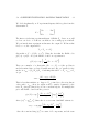


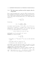

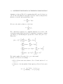


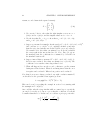
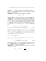


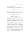
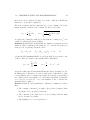
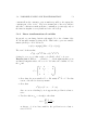


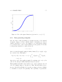


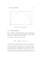


![シャープゲル[中性ゲル]](http://vs1.manualzilla.com/store/data/006625637_2-61406c4c36a06fc0479c5a9c3ecf69ca-150x150.png)