Download BayPass version 1.0 User Manual

August 4, 2015
BayPass version 1.0
User Manual
c INRA
BayPass code c Mathieu Gautier 2015
This document Contents
1 Overview
4
2 Before you start
2.1 How to get BayPass? . . . . . . . . . . . . . . . . . . . . . .
2.2 How to compile BayPass? . . . . . . . . . . . . . . . . . . . .
2.3 Input file format . . . . . . . . . . . . . . . . . . . . . . . . .
2.3.1 The genotyping data file [always required] . . . . . . . . .
2.3.2 The pool (haploid) size file [only required for Pool–Seq data]
2.3.3 The covariate data file [required for the covariate modes] . .
2.3.4 The covariance matrix file [optional, required for the AUX
covariate mode] . . . . . . . . . . . . . . . . . . . . . . .
4
4
5
6
7
8
8
3 Running BayPass
3.1 Overview of the different models available in BayPass
3.1.1 The core model . . . . . . . . . . . . . . . . . .
3.1.2 The standard covariate model and extensions .
3.1.3 The auxiliary covariate model . . . . . . . . . .
3.2 Detailed overview of all the options . . . . . . . . . . .
3.3 Format of the output files . . . . . . . . . . . . . . . .
4 Miscellaneous R functions
4.1 The R function simulate.baypass() . . .
4.1.1 Description . . . . . . . . . . .
4.1.2 Usage . . . . . . . . . . . . . .
4.1.3 Arguments (in alphabetic order)
4.1.4 Values . . . . . . . . . . . . . .
4.1.5 Examples . . . . . . . . . . . .
4.2 The R function fmd.dist() . . . . . . .
4.2.1 Description . . . . . . . . . . .
4.2.2 Usage . . . . . . . . . . . . . .
4.2.3 Arguments . . . . . . . . . . . .
4.2.4 Values . . . . . . . . . . . . . .
4.2.5 Example . . . . . . . . . . . . .
4.3 The R function geno2YN() . . . . . . .
4.3.1 Description . . . . . . . . . . .
4.3.2 Usage . . . . . . . . . . . . . .
4.3.3 Arguments . . . . . . . . . . . .
4.3.4 Values . . . . . . . . . . . . . .
4.3.5 Example . . . . . . . . . . . . .
2
.
.
.
.
.
.
.
.
.
.
.
.
.
.
.
.
.
.
.
.
.
.
.
.
.
.
.
.
.
.
.
.
.
.
.
.
.
.
.
.
.
.
.
.
.
.
.
.
.
.
.
.
.
.
.
.
.
.
.
.
.
.
.
.
.
.
.
.
.
.
.
.
.
.
.
.
.
.
.
.
.
.
.
.
.
.
.
.
.
.
.
.
.
.
.
.
.
.
.
.
.
.
.
.
.
.
.
.
.
.
.
.
.
.
.
.
.
.
.
.
.
.
.
.
.
.
.
.
.
.
.
.
.
.
.
.
.
.
.
.
.
.
.
.
.
.
.
.
.
.
.
.
.
.
.
.
.
.
.
.
.
.
.
.
.
.
.
.
.
.
.
.
.
.
.
.
.
.
.
.
.
.
.
.
.
.
.
.
.
.
.
.
.
.
.
.
.
.
.
.
.
.
.
.
.
.
.
.
.
.
.
.
.
.
.
.
.
.
.
.
.
.
.
.
.
.
.
.
.
.
.
.
.
.
9
.
.
.
.
.
.
10
10
10
11
12
15
21
.
.
.
.
.
.
.
.
.
.
.
.
.
.
.
.
.
.
24
25
25
25
25
27
29
29
29
29
29
30
30
30
30
30
30
30
31
5 Worked Examples
5.1 Cattle allele count data . . . . . . . . . . . . . . . . . . . . .
5.1.1 Analysis under the core model mode: MCMC is run
under the core model . . . . . . . . . . . . . . . . . .
5.1.2 Analysis under the IS covariate mode: MCMC is run
under the core model . . . . . . . . . . . . . . . . . .
5.1.3 Analysis under the MCMC covariate mode: MCMC is
run under the STD model . . . . . . . . . . . . . . .
5.1.4 Analysis under the AUX covariate mode: MCMC is
run under the AUX model . . . . . . . . . . . . . . .
5.2 Littorina Pool–Seq read count data . . . . . . . . . . . . . .
31
. 31
. 31
. 33
. 34
. 35
. 36
6 Copyright
36
7 Contact
36
Bibliography
37
3
1
Overview
The package BayPass is a population genomics software which is primarily
aimed at identifying genetic markers subjected to selection and/or associated
to population-specific covariates (e.g., environmental variables, quantitative
or categorical phenotypic characteristics). The underlying models explicitly
account for (and may estimate) the covariance structure among the population allele frequencies that originates from the shared history of the populations under study. Note that, apart from standard population genetics studies, BayPass is generic enough to be also suited to the analyses of data from
other kinds of experiments in which the allele frequency covariance structure
is simpler (e.g., experimental evolution). The genetic data typically consists
of allele (when derived from individual genotype calls) or read (when derived
from Pool–Seq experiments) counts at several markers (for now, BayPass is
restricted to the analysis of bi–allelic markers) in several populations. Note
that BayPass can handle missing data (no count available in one or several
populations) which might be helpful in some contexts.
The core BayPass model is based on the Bayenv model which was
proposed by Coop et al. (2010) and G¨
unther and Coop (2013). However,
as detailed in Gautier (2015), in addition to a complete and independant
reprogramming of the core Markov Chain Monte Carlo (MCMC) algorithm,
BayPass allows to monitor most of the parameters and the priors of the
original models and to introduce various extensions (via e.g., the optional
addition of hyper–parameters, the modeling of spatial dependency among
consecutive markers).
BayPass is written in Fortran90. The source code and compilation instructions for various platforms (OS X, Windows, Linux) are available. The
executable reads data file(s) supplied by the user, and a number of options
can be passed through the command line. Some R functions are also provided
in the package to facilitate interpretation of the resulting outputs.
This document provides information about how to format the data file,
how to specify the user-defined parameters, and how to interpret the results.
2
2.1
Before you start
How to get BayPass?
Download the archive from http://www1.montpellier.inra.fr/CBGP/software/
baypass/, and extract it from a terminal:
unzip baypass_1.0.zip
4
The following pre-compiled binaries are to be found in the bin subdirectory:
• BayPass.exe: a Windows binary (compiled in Windows XP virtual
machine)
• i_baypass: a 64-bit Linux binary compiled under a 64–bit Debian
wheezy with the intelr Fortran compiler ifort1
• g_baypass: a 64-bit Linux binary compiled under a 64–bit Debian
wheezy with the free compiler gfortran2 .
However, you may need to recompile using the provided source files (see the
next subsection).
2.2
How to compile BayPass?
The source files are to be found in the src subdirectory. BayPass is coded
in Fortran90 and standard options should work for most of F90 compilers.
Here are example of instructions3 for
• the gfortran free compiler :
gfortran -ffast-math -funroll-loops -O3 -Wconversion -fdefault-real-8 \
-fdefault-double-8 -ffree-line-length-none baypass.f90 -o baypass
• the ifort intelr Fortran compiler:
ifort -r8 -nowarn baypass.f90 -o baypass
1
http://software.intel.com/en-us/fortran-compilers
http://gcc.gnu.org/onlinedocs/gfortran
3
From my (limited) experience, I would recommend using the ifort intelr Fortran.
Indeed, although gfortran options could surely probably be better adapted to further
improve the speed of the executable (any feedback about this is welcome), using these
these options the ifort executable was more than two times faster than the gfortran one.
However, I noticed that the ifort executable might sometimes crash in an unpredictable
way when reading the command line arguments (for a reason that remains very obscure
to me and that I am trying to figure out!).
2
5
Under Linux (or MacOS), before the first use, make sure to give appropriate execution
rights to the program. For instance you may run:
chmod +x baypass
In the following, it is assumed that the program was made executable and accessible in
your path. For instance, under Linux, this may be achieved by copying the executable
in a directory declared in the path (e.g., /usr/local/bin) or by adding the program
to the $PATH system variable (using the export command)
2.3
Input file format
Depending on the type of analyses, different data files might be required by
the program. The following examples of the different input files are available
in the examples directory:
• geno.bta14: this file contains allele count data for 18 French cattle
breeds at 1,394 SNPs mapping to the BTA14 bovine chromosome (see
Gautier (2015) for details).
• bta.pc1: this file contains the SMS (Synthetic Morpholy Score) for the
18 French cattle breeds (see Gautier (2015) for details).
• omega.bta: this file contains the matrix Ω for the 18 French catb bpas ) as estimated under the core model from the whole
tle breeds (Ω
BTA
genome SNP data (see Gautier (2015) for details).
• lsa.geno: this file contains read count data (Pool–Seq data) for 12
populations from the Littorina saxatilis marine snail (Westram et al.,
2014) at 2,500 SNPs randomly chosen among the ones analysed in Gautier (2015) (but including the ca. 150 outlier SNPs identified).
• lsa.poolsize: this file contains the haploid pool sizes of the 12 Littorina saxatilis populations.
• lsa.ecotype: this file contains the code for the ecotype of the 12
Littorina saxatilis populations (−1 for the ”crab” habitat and 1 for the
”wave” habitat).
6
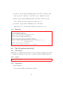
2.3.1
The genotyping data file [always required]
The genotyping data files contain allele or read count (for PoolSeq experiment) data for each of the nsnp markers assayed in each of the npops populations sampled. The genotyping data file is simply organised as a matrix with
nsnp rows and 2 ∗ npop columns. The row field separator is a space. More
precisely, each row corresponds to one marker and the number of columns is
twice the number of populations because each pair of numbers corresponds to
each allele (or read counts for PoolSeq experiment) counts in one population4 .
As a schematic example, the genotyping data input file for allele count
data should read as follows:
--- file
81 19 86
89 11 81
89 11 91
begins here --14 2 98 8 92 32 68 23 77
19 9 91 1 99 27 73 27 73
9 0 0 15 85 77 23 80 20
[...97 more lines...]
--- file ends here --In this example, there are 6 populations and 100 SNP markers. At the first
SNP, in the first population, there are 81 copies of the first allele, and 19
copies of the second allele. In the second population, there are 86 copies of
the first allele, and 14 copies of the second allele, etc. Note that both alleles
in the third SNP in the third population have 0 copie. This marker will be
treated as a missing data in the corresponding population. The file named
geno.bta14 in the example directory provides a more realistic example.
Similarly, as a schematic example, the genotyping data input file for allele
count data should read as follows:
--- file begins here --71 8 115 0 61 36 51 39 10 91 69 58
82 0 91 0 84 14 24 57 28 80 18 80
93 28 112 30 0 0 0 113 33 68 0 106
[...97 more lines...]
--- file ends here --In this example, there are also 6 populations and 100 SNP markers. At
the first SNP, in the first population, there are 71 reads of the first allele, and
4
For now, BayPass is restricted to bi–allelic marker
7
8 reads of the second allele. In the second population, there are 115 reads
of the first allele, and 0 read of the second allele, etc. Note that both alleles
in the third SNP in the third population have 0 copie. This marker will be
treated as a missing data in the corresponding population. The file named
lsa.geno in the example directory provides a more realistic example.
For Pool–Seq data to be analyzed properly (i.e. not like allele count data), it is
necessary to provide a file with the (haploid) size of each pool (see 2.3.2).
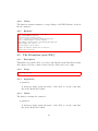
2.3.2
The pool (haploid) size file [only required for Pool–Seq data]
For Pool–Seq experiment, the haploid size (twice the number of pooled individuals for diploid species) of each population should be provided. As a
schematic example, the pool (haploid) size file should read as follows:
--- file begins here --60 75 100 90 80 50
--- file ends here --In this example, there are 6 populations with respective haploid sample
sizes of 60 (first population), 75 (second population), 100 (third population),
90 (fourth population), 80 (fifth population) and 50 (sixth population). The
order of the populations in the pool size file must be the same as in the allele
count (and the covariate) data file(s). The file named lsa.poolsize in the
example directory provides a more realistic example.
2.3.3
The covariate data file [required for the covariate modes]
The values of the covariates (e.g., environmental data, phenotypic traits, etc.)
for the different populations should be provided in a file with the format
exemplified in the following:
--- file begins here --150 1500 800 300 200 2500
181.5 172.6 152.3 191.8 154.2 166.8
1 1 0 0 1 1
0.1 0.8 -1.15 1.6 0.02 -0.5
--- file ends here --In this example, there are 6 populations (columns) and 4 covariates (row).
The first covariate might be viewed as a typical environmental covariate, like
altitude in meters (the first population is living at ca. 150m above the sea
level, the second at ca. 1,500m, and so on), the second as a quantitative traits
8
like average population sizes in cm (individuals from the first population are
181.5 cm height on average, individuals from the second population 172.6
cm, and so on), the third covariate as a typical binary trait like presence (1,
for the first, second, fifth and sixth populations) or absence (0, for the thrid
and fourth populations) and the last might be viewed as a synthetic variable
like the first principal components of a PCA. The order of the populations
(columns) in the covariate data file must be the same as in the allele count
(and the pool size) data file(s).
The files named bta.pc1 and lsa.ecotype in the example directory provide alternative real-life examples.
Note that in most cases, it is (strongly) recommended to scale each covariate (so that
c2 = 1 for each covariable). The scalecov option allows to perform this
µ
ˆ = 0 and σ
step automatically prior to analysis, if needed.
2.3.4
The covariance matrix file [optional, required for the AUX covariate mode]
For some applications (see below), it might be interesting (e.g., to parallelize
some analyses) or required (when using the AUX covariate mode) to provide
the population covariance matrix Ω. As a schematic example, the covariance
matrix file reads as follows:
--- file begins here --0.098053 0.019595 0.032433 -0.029601
0.019595 0.160147 0.018942 -0.027348
0.032433 0.018942 0.149962 -0.054973
-0.029601 0.027348 0.054973 0.187511
-0.024190 0.039733 0.058700 0.221914
-0.029247 0.039010 0.057288 0.165862
--- file ends here ---
-0.024190 -0.029247
-0.039733 -0.039010
-0.058700 -0.057288
0.221914 0.165862
0.562666 0.260231
0.260231 0.219761
In this example, there are 6 populations. Hence, the population covariance matrix is a 6×6 squared symmetric matrix. The order of the populations
(columns and rows) in the matrix Ω should be the same as the columns in
the allele count (and the pool size and the covariate) data file(s). Note that
this file is produced in the appropriate format by the program when running
BayPass under the core model (see 3.3).
The file named omega.bta provides a real-life example.
9
3
Running BayPass
3.1
Overview of the different models available in BayPass
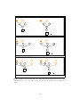
Directed Acyclic Graphs (DAG) of the different family of models are represented in Figure 1 (see Gautier (2015) for details). Briefly, three types of
(closely related) models might be investigated using BayPass, considering
either Allele count data (left panel in Figure 1) or Read count data (right
panel in Figure 1) as obtained from Pool–Seq experiments.
3.1.1
The core model
The core model depicted in Figure 1A might be viewed as a generalisation
of the model proposed by Nicholson et al. (2002) and was first proposed by
Coop et al. (2010). This model is the one considered by BayPass when no
covariate data file is provided and is actually nested in the others models.
The main parameter of interest is the (scaled) covariance matrix of population allele frequencies Ω resulting from their (possibly unknown and complex) shared history. Conversely, one might rely on this matrix for demographic inference. For instance, Ω might easily be converted (e.g., using
the cov2cor() function in R stats package) into a correlation matrix Σ further interpreted as a similarity matrix. From this latter matrix, one may
define a distance (dissimilarity) matrix (e.g., dij = 1− | ρij | where dij is
the distance between populations i and j and ρij is the element ij of Σ) to
perform hierarchical clustering5 and summarise the history of the population as a bifurcating phylogenetic tree (without gene flow). A more complex
demographic inference based on an interpretation the matrix Ω (although
estimated in a less accurate way) in terms of tree with migration has been
recently proposed by Pickrell and Pritchard (2012).
The core model allows to perform genome scan for differentiation (covariatefree) using the XtX statistics as introduced by G¨
unther and Coop (2013)
which is computed by default in BayPass. The main advantage of this
approach stems is to explicitly account for the covariance structure in population allele frequencies (via estimating Ω) resulting from the demographic
history of the populations. To identify outlier loci (based on the XtX statistics), the R function simulate.baypass() provided in the utils directory
of the package (see 4) allows to simulate data under the inference model (e.g.,
using posterior estimates of Ω and any other hyperparameters) which might
5
For an interesting discussion and examples in R, see http://research.
stowers-institute.org/mcm/efg/R/Visualization/cor-cluster/index.htm
10
further be analysed to calibrate the neutral XtX distribution (Gautier, 2015).
In the current implementation of BayPass, the prior distribution for Ω is an InverseWishart: Ω ∼ W−1
J (ρIJ , ρ) (where J is the number of populations). By default ρ = 1
(rather than ρ = J as in Bayenv) which was found as the most reliable value (Gautier,
2015). Similarly, the hyperparameters aπ and bπ of the prior β distribution for the
overall (across population) SNP allele frequencies are estimated by default. However,
they might be fixed to aπ = bπ = 1 (as in e.g., Bayenv) using fixpibetapar option
or to any other values using further the betapiprior option (3.2).
3.1.2
The standard covariate model and extensions
The standard covariate model is represented in Figure 1B and is the one
considered by default in BayPasswhen a covariate data file is provided using efile option (3.2). This model allows to evaluate to which extent the
population covariable(s) k is (linearly) associated to each marker i (which
are assumed independant given Ω) by the introduction of the regression coefficients βik (for convenience the indices k for covariables are dropped in
Figure 1B).
In the current implementation of BayPass, the prior distribution for the βik ’s is
Uniform: βik ∼ Unif (βmin , βmax ). By default, βmin = −0.3 and βmax = 0.3 but
these values might be changed by the user with the minbeta and maxbeta options
respectively (3.2). Note that in Bayenv (Coop et al., 2010), βmin = −0.1 and βmax =
0.1.
The estimation of the βik regression coefficients for each SNP i may be
performed using two different approaches (Gautier, 2015):
• Using an importance sampling estimator (IS) which is the default option and also allows the computation of Bayes Factor to the compare on
an individual SNP (and covariable) basis the two alternative models,
namely the model with association (βik 6= 0) against the null model
(βik = 0). Bayes Factor (BFis ) and βik IS algorithm are inspired from
Coop et al. (2010) and are described in details elsewhere (Gautier,
2015). Note that the IS estimation procedure is based on a numerical
integration that requires the definition of a grid covering the whole support of the βik prior distribution. In BayPass, the grid consists in nβ
(by default nβ = 201) equidistant points from βmin to βmax (including
the boundaries) leading to a lag between two successive values equal to
βmax −βmin
(i.e., 0.003 with default values). Other values for nβ might be
nβ −1
supplied by the user with the nbetagrid option (3.2).
• Using an MCMC algorithm (activated via the covmcmc option). In
this case, the user should provide the matrix Ω (e.g., using posterior
11
estimates available from a previous analysis) and it is recommended to
consider only one covariable at a time (particularly if some covariables
are correlated).
3.1.3
The auxiliary covariate model
The auxiliary covariate model, represented in Figure 1C and activated with
the auxmodel option, is an extension of the previous model (Figure 1B) involving the introduction of a Bayesian (binary) auxiliary variable δik for each
regression coefficient βik (Gautier, 2015). In a similar population genetics
context, this modelling was also proposed by Riebler et al. (2008) to identify
markers subjected to selection in genome-wide scan of adaptive differentiation based on a F–model.
Here, the auxiliary variable actually indicates whether a specific SNP i can
be regarded as associated to a given covariable k (δik = 1) or not (δik = 1).
By looking at the posterior distribution of each auxiliary variable, it is then
straightforward to derive a Bayes Factor (BFmc ) to compare both models
while dealing with multiple testing issues (Gautier, 2015). In addition, the
introduction of a Bayesian auxiliary variable makes it easier to account for
spatial dependency among markers. In BayPass, the general form of the δik
prior distribution is indeed that of an 1D Ising model with a parametrization
analogous to the one proposed in a similar context by Duforet-Frebourg et al.
(2014): π (δk ) ∝ P s1 (1 − P )s0 eηβisg , where δk is the vector of the nsnp auxiliary variables for covariable k, s1 and s0 are the number of SNPs associated
(i.e. with δik = 0) and not associated (i.e. with δik = 0) to the covariable6 ,
and η corresponds to the number of pairs of consecutive markers (neighbors)
that are in the same state at the auxiliary variable7 (i.e., δi,k = δi+1,k ). The
parameter P broadly corresponds to the prior proportion of SNP associated
to the covariable. In the BayPass auxiliary model, P is assumed a priori
beta distributed: P ∼ β (aP , bP ). By default, aP = 0.02 and bP = 1.98 (this
values might be changed by the user with the auxPbetaprior option) which
P
=1%) are
amounts to consider that only a small fraction of the SNPs ( aPa+b
P
a priori expected to be associated to the covariable while allowing some uncertainty on this key parameter (e.g., the prior probability of P >10% being
equal to 0.028 with these parameters). The parameter βisg , called the inverse temperature in the Ising (and Potts) model literature, determines the
level of spatial homogeneity of the auxiliary variables between neighbors. In
6
s1 =
nsnp
P
δik = 1 and s0 =
i=1
P
7
η=
1δik =δjk
nsnp
P
δik = 0
i=1
i∼j
12
BayPass, βisg = 0 by default implying that auxiliary variables are independent (no spatial dependency). Note that βisg = 0 amounts to assume the
δik follows a Bernoulli distribution with parameter P . Conversely, βisg > 0
leads to assume that the δik with similar values tend to cluster according
to the underlying SNP positions (the higher the βisg , the higher the level of
spatial homogeneity). In biological terms, SNP associated to a given covariable might be expected to cluster due to Linkage Disequilibrium with the
underlying (possibly not genotyped) causal variant(s). In practice, βisg = 1
is commonly used and a value of βisg ≤ 1 is recommended.
In technical terms, the overall parametrisation of the Ising prior assumes no external
field and no weight (as in the so-called compound Ising model) between the neighboring auxiliary variables. In the current implementation of the BayPass auxiliary
covariate model (when βisg > 0), the information about the distances between SNPs
is therefore not accounted for. Only the relative position of markers are considered.
For the applications where this modeling might be relevant (whole genome scan), this
corresponds to assuming a relative homogeneity in marker spacing as measured by
genetic (rather than physical) distances (which might be unavailable, in practice).
13
A) Basic Model (without covariate)
A.2) Read count data (Pool–Seq)
A.1) Allele count data
aπ
aπ +bπ ∼ U(0; 1)
πi
aπ
aπ +bπ ∼ U(0; 1)
aπ + bπ ∼ Exp(1)
∼ β (aπ ; bπ )
Ω
−1
ρIJ , ρ
∼ W
J
πi
aπ + bπ ∼ Exp(1)
∼ β (aπ ; bπ )
∼ NJ πi IJ ; πi (1 − πi )Ω
α?i
yij , nij
yij ∼ Bin min(1, max(0, α?
ij )); nij
−1
ρIJ , ρ
∼ W
J
Ω
α?i
∼ NJ πi IJ ; πi (1 − πi )Ω
yij
∼ Bin min(1, max(0, α?
ij )); nj
rij , cij
rij ∼ Bin
yij
, cij
nj
B) Standard (STD) covariate model
B.2) Read count data (Pool–Seq)
B.1) Allele count data
aπ
aπ +bπ ∼ U (0; 1)
πi
aπ
aπ +bπ ∼ U (0; 1)
aπ + bπ ∼ Exp(1)
−1
∼ W
ρIJ , ρ
J
Ω
∼ β (aπ ; bπ )
α?i
∼ NJ
yij , nij
βi
∼ U βmin ; βmax
πi
aπ + bπ ∼ Exp(1)
∼ β (aπ ; bπ )
πi IJ + βi pj ; πi (1 − πi )Ω
yij ∼ Bin min(1, max(0, α?
ij )); nij
−1
∼ W
ρIJ , ρ
J
Ω
βi
∼ U βmin ; βmax
πi IJ + βi pj ; πi (1 − πi )Ω
α?i
∼ NJ
yij
∼ Bin min(1, max(0, α?
ij )); nj
rij , cij
rij ∼ Bin
yij
, cij
nj
C) Auxiliary variable (AUX) covariate model
C.1) Allele count data
aπ
aπ +bπ
πi
C.2) Read count data (Pool–Seq)
aπ + bπ
Ω
βi
α?i
yij , nij
∼ U βmin ; βmax
∼ NJ
P
∼ β a p ; bp
δ
∼ Ising isβ ; P
aπ
aπ +bπ
πi
πi IJ + δi βi pj ; πi (1 − πi )Ω
yij ∼ Bin min(1, max(0, α?
ij )); nij
aπ + bπ
Ω
βi
∼ U βmin ; βmax
∼ β ap ; bp
δ
∼ Ising isβ ; P
πi IJ + δi βi pj ; πi (1 − πi )Ω
α?i
∼ NJ
yij
∼ Bin min(1, max(0, α?
ij )); nj
rij , cij
P
rij ∼ Bin
yij
, cij
nj
Figure 1: Directed Acyclic Graphs of the different hierarchical Bayesian models available
in BayPass (see 3.1). For each model, optional (hyper–)parameters are displayed in
orange.
14
3.2
Detailed overview of all the options
BayPass is a command-line executable. The ASCII hyphen-minus (”-”) is
used to specify options. As specified below, some options take integer or float
values and some options do not. Here is an example call of the program:
baypass -npop 12 -gfile data.geno -efile env.data -outprefix ana1
The full list of the options accepted by BayPass are printed out using the command: baypass -help as follows:
Version 1.0
Usage: BayPass [options]
Options:
I)
General Options:
-help
-npop
INT
-gfile
CHAR
-efile
CHAR
-scalecov
CHAR
-poolsizefile
CHAR
-outprefix
CHAR
II) Modeling Options:
-omegafile
CHAR
-rho
INT
-setpibetapar
-betapiprior
FLOAT2
-minbeta
FLOAT
-maxbeta
FLOAT
Display the help page
Number of populations
Name of the Genotyping Data File
Name of the covariate file: activate covariate mode
Scale covariates
Name of the Pool Size file => activate PoolSeq mode
Prefix used for the output files
Name of the omega matrix file => inactivate estim. of omega
Rho parameter of the Wishart prior on omega
Inactivate estimation of the Pi beta priors parameters
Pi Beta prior parameters (if -fixpibetapar)
Lower beta coef. for the grid
Upper beta coef. for the grid
(always required)
(always required)
(def="")
(def="")
(def="")
(def="")
(def="")
(def=1)
(def=1.0 1.0)
(def=-0.3)
(def= 0.3)
I.1) IS covariate mode (default covariate mode):
-nbetagrid
INT
Number of grid points (IS covariate mode)
(def=201)
I.2) MCMC covariate mode:
-covmcmc
Activate mcmc covariate mode (desactivate estim. of omega)
-auxmodel
Activate Auxiliary variable mode to estimate BF
-isingbeta
FLOAT Beta (so-called inverse temperature) of the Ising model
-auxPbetaprior
FLOAT2 auxiliary P Beta prior parameters
(def=0.0)
(def=0.02 1.98)
III) MCMC Options:
-nval
INT
-thin
INT
-burnin
INT
-npilot
INT
-pilotlength
INT
-accinf
FLOAT
-accsup
FLOAT
-adjrate
FLOAT
-d0pi
FLOAT
-upalphaalt
-d0pij
FLOAT
-d0yij
INT
-seed
INT
Number of post-burnin and thinned samples to generate
Size of the thinning (record one every thin post-burnin sample)
Burn-in length
Number of pilot runs (to adjust proposal distributions)
Pilot run length
Lower target acceptance rate bound
Upper target acceptance rate bound
Adjustement factor
Initial delta for the pi all. freq. proposal
Alternative update of the pij
Initial delta for the pij all. freq. proposal (alt. update)
Initial delta for the yij all. count (PoolSeq mode)
Random Number Generator seed
(def=1000)
(def=25)
(def=5000)
(def=20)
(def=1000)
(def=0.25)
(def=0.40)
(def=1.25)
(def=0.5)
(def=0.05)
(def=1)
(def=5001)
In this menu, each option is followed by the kind of argument (if any)
required (e.g., INT for integer, FLOAT for real, FLOAT2 for a pair of real
number space separated), a brief description of its function, and the default
value.
In the following, we detailed all the options of BayPass:
-help
This option prints out the help menu (see above). Note that this option
is dominating all the other options, i.e. if -help is used in conjunction
15
with any other option of the program, the help menu is displayed. No
argument is required for this option.
-npop
This option (mandatory) gives the number of population considered
in the data set (half the number of column in the genotype data file).
The required argument must be an integer (INT). (e.g., -npop 12 if 12
populations are studied).
-gfile
This option (mandatory) gives the name of the genotyping input file.
See 2.3.1 for a description of the corresponding input file format. The
required argument must be character chain (name of the input file)
without space (e.g., -gfile data.geno if the input file is named ”data.geno”).
-efile
This option gives the name of the covariate input file. See 2.3.3 for a
description of the corresponding input file format. The required argument must be character chain (name of the input file) without space
(e.g., -gfile data.env if the input file is named ”data.env”).
-scalecov
This option allows to perform scaling of each covariable in the covariate
input file (See 2.3.3). No argument is required for this option. If
activated, an output file named ”covariate.std” containing the scaled
covariables is produced.
-poolsizefile
This option gives the name of the input file containing the haploid sample size of each population. See 2.3.2 for a description of the corresponding input file format. The required argument must be character chain
(name of the input file) with no space (e.g., -poolsizefile data.poolsize
if the input file is named ”data.poolsize”). Note that this option automatically activates the Pool–Seq mode, i.e., the PoolSeq version of the
different models are considered (as represented in Figures 1A2, B2 and
C2).
-outprefix
16
This option allows to add a prefix to all the output files. The required
argument must be a character chain without space. For instance, if
using -outprefix ana1, the name of all the output files will begin by
”ana1_”. By default, no prefix is added.
-omegafile
This option gives the name of the input file for the population covariance matrix (Ω in 3.1.1 and Figure 1). See 2.3.4 for a description of the corresponding input file format. The required argument
must be character chain (name of the input file) with no space (e.g.,
-omegafile matrix.dat if the input file is named matrix.dat). This
option inactivates the estimation of Ω and is mandatory in the covariate models involving estimation of the regression coefficients via
MCMC i.e. the standard model (see 3.1.2) with the -covmcmc option
and the auxiliary variable model (see 3.1.3).
-rho
This option allows to specify the value of ρ for the Inverse-Wishart
prior of Ω (see Figure 1 and 3.1.1). The required argument must be a
positive integer. By default, -rho 1 (i.e., ρ = 1).
-setpibetapar
This option allows to inactivate estimation of the two (hyper–)parameters
aπ and bπ of the prior β distribution for the overall (across population)
SNP allele frequencies (see Figure 1 and 3.1.1) (and set them to the values specified with the -betapiprior option). No argument is required
for this option.
-betapiprior
This option allows to specify the values of the two (hyper–)parameters
aπ and bπ (respectively) of the prior β distribution for the overall
(across population) SNP allele frequencies (see Figure 1 and 3.1.1).
The required argument must be two positive real numbers. By default
-betapiprior 1.0 1.0 (i.e., aπ = bπ = 1).
-minbeta
This option allows to specify the lower bound of the Uniform prior
distribution on the regression coefficients (see Figure 1 and 3.1.2). The
17
required argument must be a real number (lower than maxbeta defined
below). By default -minbeta -0.3 (i.e., βmin = −0.3).
-maxbeta
This option allows to specify the upper bound of the Uniform prior
distribution on the regression coefficients (see Figure 1 and 3.1.2). The
required argument must be a real number (greater than minbeta defined above). By default -maxbeta 0.3 (i.e., βmax = 0.3).
-nval
This option gives the number of post–burn–in (and thinned MCMC)
samples recorded from the posterior distributions of the parameters of
interest. The required argument must be a positive integer. By default, -nval 1000 (i.e., 1,000 post burn-in and thinned samples are
generated). Note that with default values, the total number of iterations of the MCMC sampler run after the burn-in period is equal to
25,000 (since by default, the thinning rate is equal to 25 , see thin
option)
-thin
This option gives the size of the thinning (i.e., the number of iterations
between any two records from the MCMC). The required argument
must be a positive integer. By default, -thin 25 (i.e., the size of the
thinning is 25).
-burnin
This option gives the length of the burn-in period (i.e., the number
of iterations before the first record from the MCMC). The required
argument must be a positive integer. By default, -burnin 5000 (i.e.,
5,000 iterations are run during the burn–in period).
-npilot
This option gives the number of pilot runs (i.e., the number of runs
used to adjust the parameters of the MCMC proposal distributions of
parameters updated through a Metropolis-Hastings algorithm). The
targeted acceptance rates are defined with the accinf and accsup options (by default, these are set to 0.25 and 0.40 respectively). The
required argument must be a positive integer. By default, -npilot 20
(i.e., 20 pilot runs are performed).
18
-pilotlength
This option gives the number of iterations of each pilot run (see npilot
option above). The required argument must be a positive integer. By
default, -pilotlength 1000 (i.e., each pilot run consist of 1,000 iterations).
-accinf
This option gives the lower bound of the targeted acceptance rates to
adjust the parameters of the MCMC proposal distributions of parameters updated through a Metropolis-Hastings algorithm, during the pilot
runs. For instance, in the case of a uniform proposal distribution of the
form Unif(x − δ, x + δ) (where x represents the current value of the parameter of interest and δ specifies the size of the support), if acceptance
rates are below this lower bound after a pilot run, then δ is increased
(e.g., multiplied by a factor defined with the adjrate parameter and
set to 1.25 by default). The required argument must be a positive
real number (< 1 and lower than accsup defined below). By default,
-accinf 0.25 (i.e., acceptance rates should be at least equal to 25%).
-accsup
This option gives the upper bound of the targeted acceptance rates
to adjust the parameters of the MCMC proposal distributions of parameters updated through a Metropolis-Hastings algorithm, during the
pilot runs. For instance, in the case of a uniform proposal distribution
of the form Unif(x − δ, x + δ) (where x represents the current value
of the parameter of interest and δ specifies the size of the support), if
acceptance rates are above this upper bound after a pilot run, then δ is
decreased (e.g., divided by a factor defined with the adjrate parameter
and set to 1.25 by default). The required argument must be a positive
real number (≤ 1 and greater than accinf defined above). By default,
-accinf 0.40 (i.e., acceptance rates should be less than 40%).
-adjrate
This option gives the factor used to adjust the parameters of the MCMC
proposal distributions of parameters updated through a MetropolisHastings algorithm, during the pilot runs. For instance, in the case of
a uniform proposal distribution of the form Unif(x − δ, x + δ) (where x
represents the current value of the parameter of interest and δ specifies
19
the size of the support), if acceptance rates are below (respectively
above) the lower (respectively upper) bound of the targeted regions (as
defined above with the accinf and accsup options) after a pilot run,
then δ is multiplied (respectively, divided) by this factor. The required
argument must be a real number > 1. By default, -adjrate 1.25.
-d0pi
This option gives the initial value of the δπ , which is half the window
width from which proposal values of the overall SNP allele frequencies
πi (see Figure 1) are drawn uniformly around the current value pij in the
Metroplis–Hastings update. The value of δπ is eventually adjusted for
each locus during the pilot runs (see options -npilot, -pilotlength,
-accinf, -accsup and -adjrate). The required argument must be a
positive real number. By default, -d0pi 0.5 (i.e., δp = 0.5).
-upalphaalt
This option activates an alternative Metropolis–Hastings algorithm for
the population SNP allele frequencies αij (see Figure 1). By default,
the proposal is the same as the one described by Coop et al. (2010)
(Appendix A). Briefly, denoting αi. as the vector of allele frequencies
for SNP i in each population, the vector α? cdt
evaluated in a given
i
Metropolis–Hastings update is sampled from the following multivariate
Gaussian distribution: α? cdt
∼ M N V (α? i , Γσi2 ) where Γ is obtained
i
by a Choleski decomposition of the matrix Ω (i.e., Ω = t ΓΓ ). The alternative proposal activated with the -upalphaalt option is defined on
a SNP by population basis and is a uniform distribution centred on the
?
α
?
α
current values of the parameters (i.e., α? cdt
ij ∼ Unif(α ij −λij , αij −λij )).
The algorithm is slower than the default one but may perform better,
in particular when sample sizes are heterogeneous across samples. No
argument is required for this option.
-d0pij
This option gives the initial value of the δα used in the proposal distribution of the population SNP allele frequencies αij in the Metroplis–
Hastings updates. Following the notations used above (see -upalphaalt
option), δα = σi2 for the default algorithm and δα = λαij for the alternative algorithm. The value of δα is eventually adjusted for each locus
(and population, in the case of the alternative algorithm) during the pilot runs (see options -npilot, -pilotlength, -accinf, -accsup and
20
-adjrate). The required argument must be a positive real number.
By default, -d0pij 0.05 (i.e., σi2 = 0.05 for the default algorithm and
λαij = 0.05 for the alternative algorithm).
-d0yij
This option gives, in the Pool–Seq mode, the initial value of the δy
used in the proposal distribution of the population SNP allele count
Yij in the Metroplis–Hastings updates. The value of δy is eventually
adjusted for each locus and each population during the pilot runs (see
options -npilot, -pilotlength, -accinf, -accsup and -adjrate).
The required argument must be a positive integer number lower than
the haploid pool sizes. By default, -d0yij 1 (i.e., δy = 1).
-seed
This option gives the initial seed of the (pseudo-) Random Number
Generator. The required argument must be a positive integer number.
By default, -seed 5001.
3.3
Format of the output files
While running, BayPass printed on the console several information regarding the execution of the analysis (these might be redirected in a log file using
the > log.file unix syntax). At the end of the analysis BayPass produces
several output files which might varied according to the options considered
(see 3.2). The name of these different output files might be preceded by a
prefix as defined with the outprefix options (see 3.2).
In the following, we detailed all the output files that may be generated
by BayPass:
• (outprefix_)summary_pij.out (default mode; e.g., for allele count
data) or (outprefix_)summary_yij_pij.out (Pool–Seq mode; e.g., for
read count data)
These files contain for each locus (MRK column) within each population (POP column), the mean (M_P column) and the standard deviation
?
(SD_P column) of the posterior distribution of the αij
parameter (see
Figure 1) that is closely related to the frequency of the reference allele
?
αij = 1 ∧ (0 ∨ αij
) except that its support is on the real line (hence possible values < 0 or > 1). It also contains the posterior mean (M_Pstd
column) and the standard deviation (SD_Pstd column) of the standardized allele frequency αstd (αstd = Γ−1 α? ). The final adjusted values
21
of the δα ’s, the parameters of the MCMC proposal distributions for
the SNP allele frequencies (see -upalphaalt option) are also reported
in these files (DELTA_P column) together with the post-burn–in final
acceptance rates (ACC_P column). Note that in the default Metropolis–
?
are updated for each SNP as a vector of
Hastings algorithm, the αij
allele frequencies across all populations. Hence, the δα and the acceptance rates have same values across all the populations for a given SNP.
In the Pool–Seq mode (i.e., in the (outprefix_)summary_yij_pij.out
file), the columns M_Y, SD_Y, DELTA_Y and ACC_Y similarly report the
posterior mean, the posterior standard-deviation, the δY of the corresponding proposal distributions and the post-burn–in final acceptance
rates for allele counts of each SNP within each population.
• (outprefix_)summary_pi_xtx.out
This file contains for each locus (MRK column), the mean (M_P column)
and the standard deviation (SD_P column) of the posterior distribution
of the (across populations) frequency πi of the SNP reference allele (see
Figure 1). The final adjusted values of the δπ ’s, the parameters of the
MCMC proposal distributions are also reported in these files (DELTA_P
column) together with the post-burn–in final acceptance rates (ACC_P
column). In addition, this files contains for each SNP, the posterior
mean (M_XtX column) and standard deviation (SD_XtX column) of the
XtX statistics introduced by G¨
unther and Coop (2013) to identify outlier loci in genome–scan of adaptive differentiation (see 3.1.1).
• (outprefix_)summary_lda_omega.out and (outprefix_)mat_omega.out
The (outprefix_)summary_lda_omega.out file contains the posterior
means and posterior standard deviations of each element of the npop ×
npop scaled population allele frequencies covariance matrix Ω (M_omega_ij
and SD_omega_ij columns respectively) as described in Figure 1 (see
also 3.1.1), and its inverse Λ = Ω−1 (M_lambda_ij and SD_lambda_ij
columns respectively).
The (outprefix_)mat_omega.out file contains the posterior means of
the elements of Ω in a matrix format. Note that this file is in the
format required by the -omegafile option of BayPass.
• (outprefix_)summary_beta_params.out (generated with the -estpibetapar
option)
22
This file contains the posterior mean (Mean column) and standard deviation (SD column) of the two parameters (aπ and bπ ) of the Beta
prior distribution assumed for the (across populations) frequencies of
the SNP reference allele (see Figure 1).
• (outprefix_)summary_betai_reg.out
This file is only produced in the Bayenv–like mode, i.e. the standard
covariate mode (see Figure 1B and 3.1.2) where the estimation of the
Bayes Factor (column log10(BF)) in the log–scale measuring the support of the association of each SNP with each population covariable and
the corresponding regression coefficients βi (column Beta_is) are done
via an Importance Sampling algorithm (Coop et al., 2010). In addition,
the file also contains an approximated Bayesian P–value in the log10
scale (log10(BP)) measured as lBP = −log10 (1 − 2 | 0.5 − Φ(c
µβ /c
σβ ) |)
(where Φ(x) represents the cumulative distribution function for the
standard normal distribution) and thus allowing to evaluate the support in favour of a non-null regression coefficient (e.g., lBP > 3). This
file contains for each covariable and each SNP, the posterior mean
and standard deviation of the Pearson correlation coefficient (columns
M_Pearson andSD_Pearson
respectively) between the scaled allele fref? =
quencies α
i
α? −πi
√ ij
π(1−πi )
and the given covariable after rotation
(1..J)
of both vectors by Γ−1 (see G¨
unther and Coop, 2013) where Γ is obtained by a Choleski decomposition of the matrix Ω (i.e., Ω = t ΓΓ).
• (outprefix_)summary_betai.out (generated with the -covmcmc option)
This file is produced in place of the (outprefix_)summary_betai_reg.out
described above when the -covmcmc option is activated (see 3.1.2).
Under the standard model (default), the file contains for each SNP,
the posterior mean µ
cβ (M_Beta column) and standard deviation σ
cβ
(SD_Beta column) of the regression coefficient βi together with the
adjusted δβ parameter (DeltaB column) of the proposal distribution
and the post-burn–in acceptance rate (AccRateB column). In addition,
the file also contains an approximated Bayesian P–value in the log10
scale (-logBPval) measured as lBP = −log10 (1 − 2 | 0.5 − Φ(c
µβ /c
σβ ) |)
(where Φ(x) represents the cumulative distribution function for the
standard normal distribution) and thus allowing to evaluate the support
in favour of a non-null regression coefficient (e.g., lBP > 3).
23
Under the model with auxiliary variables (-auxmodel option, see 3.1.3),
the file contains for each SNP, the posterior mean (M_Beta column) and
standard deviation (SD_Beta column) of the regression coefficient βi ,
the posterior mean of the auxiliary variable (M_Delta column) and the
estimate of the Bayes Factor (BF column) for comparison of models with
(βi 6= 0) and without (βi = 0) correlation with the given covariable.
• (outprefix_)summary_Pdelta.out (covariate model with auxiliary variable, i.e. -auxmodel option, see 3.1.3)
This file contains the posterior mean (M_P column) and standard deviation (SD_P column) of the parameter P (see Figure 1C and 3.1.3)
corresponding to the overall proportion of SNP associated to the corresponding covariable.
• (outprefix_)covariate.std (generated by the scalecov option)
This file contains the scaled covariables.
• (outprefix_)DIC.out
This files contains the average deviance (bar(D) column), the effective
number of parameters of the models (pD column) and the Deviance
Information Criterion (DIC column) as defined in Spiegelhalter et al.
(2002) and that might be relevant for model comparison purposes. In
addition, the logarithm of the pseudo-marginal likelihood of the model
is also provided (LPML column).
4
Miscellaneous R functions
The baypass_utils.R file in the utils directory contains three R functions
(R Core Team, 2015) (simulate.baypass(); fmd.dist() and geno2YN())
that may be helpful to interpret some of the results obtained with BayPass.
To use this functions, one may simply need to source the corresponding
files and ensure that the packages mvtnorm (Genz et al., 2015) and geigen
(Hasselman, 2015) have been installed. In addition, although not required by
theses functions, the packages corrplot (Wei, 2013) and ape (Paradis et al.,
2004) might proved useful for the visualisation of the Ω matrix (see 5).
24
4.1
4.1.1
The R function simulate.baypass()
Description
The R function simulate.baypass() allows to simulate either allele or read
count data under the core inference model (Figure 1A) and possibly under the
STD covariate model (Figure 1B). It produces several objects and output files
in a format directly appropriate for analyses with BayPass and Bayenv28 .
In practice, this function is useful to generate POD for calibration of the XtX
differentiation measure (or any other measures). More broadly, because the
Ω matrix capture the demographic history of the populations, this function
might also be viewed as an efficient simulator of population genetics data.
4.1.2
Usage
simulate.baypass(omega.mat,nsnp=1000,beta.coef=NA,beta.pi=c(1,1),
pop.trait=0,sample.size=100,pi.maf=0.05,suffix="sim",
remove.fixed.loci=FALSE,coverage=NA)
4.1.3
Arguments (in alphabetic order)
• beta.pi (def=c(1,1))
A two elements vector giving the parameters aπ and bπ respectively, for
the Beta distribution of the πi (”ancestral”) allele frequencies.
• beta.coef (def=NA; required for simulation under the STD covariate
model)
A vector giving the values of the regression coefficients (βi in Figure 1)
for the simulated associated SNPs (the number of the simulated associated SNPs is equal to the dimension of the vector).
• coverage (def=NA; required to activate simulation of read count data)
Either a single value or a matrix giving the total read counts. In the
latter case, the vector of total read counts for each simulated SNP
are sampled with replacement from the row of the matrix. It is thus
mandatory that the number of columns of the matrix equals the number
of populations, but no restriction are set for the number of rows. For
8
For analyses with Bayenv2, make sure fixed loci have been removed, i.e.,
remove.fixed.loci=TRUE
25
instance, if the matrix has only one row, all the SNPs will have the
same read counts within a given population.
• omega.mat (always required)
A positive definite and symmetric matrix of rank npop corresponding
to the covariance matrix of population allele frequencies (Ω in Figure 1)
• nsnp (def=1000)
A single number giving the number of (neutral) SNPs to simulate.
• pi.maf (def=0.05)
A single value giving the MAF threshold on the simulated πi (”ancestral”) allele frequencies. In the simulation procedure, the pii ’s are
sampled from the Beta distribution with parameters as specified in
the beta.pi argument. For a given SNP i, if pii <pi.maf (resp.
pii > 1−pi.maf) then pii is set equal to pi.maf (resp. 1−pi.maf).
Setting pi.maf= 0 inactivates MAF filtering.
• pop.trait (def=0; required for simulation under the STD covariate
model)
A vector of length npop giving each population-specific covariable values (ordering of the population is assumed to be the same as in the
omega.mat matrix). By default all values are set to 0 (meaning the
associated SNPs behave neutrally irrespective of their values at the
regression coefficients).
• remove.fixed.loci (def=FALSE)
A logical indicating wether or not fixed loci (in the observed simulated
data) should be discarded.
• sample.size (def=100)
If simulating allele count data, either a single value or a matrix giving
the total allele counts (twice the number of genotyped individuals in
diploid species). In the latter case, the vector of total allele counts
for each simulated SNP are sampled with replacement from the row of
the matrix. It is thus mandatory that the number of columns of the
matrix equals the number of populations, but no restriction are set for
26
the number of rows. For instance, if the matrix has only one row, all
the SNPs will have the same allele counts within a given population.
If simulating read count data, either a single value or a vector of length
npop giving the pool haploid sample sizes for each population.
• suffix (def=”sim”)
A character string giving the suffix of the output files generated by the
function.
4.1.4
Values
The function produces an object which is a list with the following components:
• omega.sim
A matrix corresponding to the one used for simulation and declared
with the omega.mat argument
• alpha.sim
A matrix with dimension nsnp rows and npop columns giving the simulated (unbounded) allele frequencies for each simulated SNP within
?
in Figure 1).
each population (i.e., αij
• pi.sim
A vector of length nsnp giving the simulated πi ”ancestral” allele frequencies for each simulated SNP.
• N.sim
A matrix with dimension nsnp rows and npop columns giving the total
allele counts for each simulated SNP within each population.
• Y.sim
A matrix with dimension nsnp rows and npop columns giving the allele counts for the reference allele for each simulated SNP within each
population.
27
• N.pool (read count data only)
A matrix with dimension nsnp rows and npop columns giving the total
read counts for each simulated SNP within each population.
• Y.pool (read count data only)
A matrix with dimension nsnp rows and npop columns giving the read
counts for the reference allele for each simulated SNP within each population.
• betacoef.sim (simulation under the STD covariate model only)
A vector of length nsnp giving the regression coefficients of each SNP
used to simulate the data.
In addition, the following output files are printed out (the extension
.suffix is as defined in the suffix argument):
• G.suffix
The allele count data file in BayPass format (see 2.3).
• Gpool.suffix (when simulating read count data)
The read count data file in BayPass format (see 2.3).
• bayenv_freq.suffix
The allele count data file in Bayenv2 format (see 8).
• bayenv_freq_pool.suffix (when simulating read count data)
The read count data file in Bayenv2 format (see 8).
• alpha.suffix
The simulated (unbounded) allele frequencies (nsnp rows and npop
?
columns) for each simulated SNP within each population (i.e., αij
in
Figure 1)
• pi.suffix
The simulated πi ”ancestral” allele frequencies for each simulated SNP.
28
• betacoef.suffix (when simulating under the STD covariate model)
The regression coefficients of each SNP used to simulate the data.
• pheno.suffix (when simulating under the STD covariate model)
The covariate data file in BayPass format (see 2.3).
• poolsize.suffix (when simulating read count data)
The haploid pool size data file in BayPass format (see 2.3).
4.1.5
Examples
#source the baypass R functions (check PATH)
source("utils/baypass_utils.R")
#load the bovine covariance matrix
om.bta <- as.matrix(read.table("examples/omega.bta"))
#simulate allele count data for 1000 SNPs
simu.res <- simulate.baypass(omega.mat=om.bta)
#simulate allele count data for 1000 neutral SNPs and
#100 associated SNPs with varying regression coefficients
simu.res <- simulate.baypass(omega.mat=om.bta,beta.coef=runif(100,-0.2,0.2),
pop.trait=rnorm(18))
#simulate read count data for 1000 SNPs
simu.res <- simulate.baypass(omega.mat=om.bta,coverage=50)
4.2
4.2.1
The R function fmd.dist()
Description
This function computes the metric proposed by (F¨orstner and Moonen, 2003)
to evaluate the distance between two covariance matrices (FMD distance).
4.2.2
Usage
fmd.dist(mat1,mat2)
4.2.3
Arguments
• mat1 and mat2
Two positive-definite (symmetric) matrices
29
4.2.4
Values
The function returns a numeric corresponding to the FMD distance between
the two matrices.
4.2.5
Example
#source the baypass R functions (check PATH)
source("utils/baypass_utils.R")
#load the bovine covariance matrix
om.bta <- as.matrix(read.table("examples/omega.bta"))
#create a dummy diagonal covariance matrix
#this might be obtained from a star-shaped phylogeny with
#branch length (Fst) equal to 0.1
star.bta<-diag(0.1,nrow(om.bta))
#compute the fmd.dist between the two matrices
fmd.dist(om.bta,star.bta)
4.3
4.3.1
The R function geno2YN()
Description
This function reads the allele (or read) count data file in the BayPass format
and extract both the counts for the reference allele and total counts.
4.3.2
Usage
geno2YN(genofile)
4.3.3
Arguments
• genofile
A character string giving the name of the allele (or read) count data
file in the BayPass format.
4.3.4
Values
The function returns two matrices:
• genofile
A character string giving the name of the allele (or read) count data
file in the BayPass format.
30
The function produces an object which is a list containing the two following matrices:
• YY
A matrix with nsnp rows and npop columns containing allele or read
counts for the reference allele.
• NN
A matrix with nsnp rows and npop columns containing the total allele
or read counts.
4.3.5
Example
#source the baypass R functions (check PATH)
source("utils/baypass_utils.R")
#load the bovine BTA 14 data
counts.obj <- geno2YN("examples/geno.bta14")
5
Worked Examples
For illustration purposes, different types of analyses of the example files
(see 2.3) are detailed step by step. Users might try to reproduce the corresponding examples using the files included in the example directory.
5.1
5.1.1
Cattle allele count data
Analysis under the core model mode: MCMC is run under
the core model
The following command allows to analyse the data under the core model (this
should take ca. 4 min with the i_baypass executable and ca. 7 min with
the g_baypass executable):
baypass -npop 18 -gfile geno.bta14 -outprefix anacore
To visualize the results, one may open an R session and proceed as follows:
require(corrplot) ; require(ape)
#source the baypass R functions (check PATH)
source("utils/baypass_utils.R")
#upload estimate of omega
omega=as.matrix(read.table("anacore_mat_omega.out"))
pop.names=c("AUB","TAR","MON","GAS","BLO","MAN","MAR","LMS","ABO",
"VOS","CHA","PRP","HOL","JER","NOR","BRU","SAL","BPN")
31
dimnames(omega)=list(pop.names,pop.names)
#Compute and visualize the correlation matrix
cor.mat=cov2cor(omega)
corrplot(cor.mat,method="color",mar=c(2,1,2,2)+0.1,
main=expression("Correlation map based on"~hat(Omega)))
#Visualize the correlation matrix as hierarchical clustering tree
bta14.tree=as.phylo(hclust(as.dist(1-cor.mat**2)))
plot(bta14.tree,type="p",
main=expression("Hier. clust. tree based on"~hat(Omega)~"("*d[ij]*"=1-"*rho[ij]*")"))
#Compare the estimate of omega based on the whole genome
#and based on the BTA14 SNPs
wg.omega <- as.matrix(read.table("examples/omega.bta")) #check the PATH
plot(wg.omega,omega) ; abline(a=0,b=1)
fmd.dist(wg.omega,omega)
#Estimates of the XtX differentiation measures
anacore.snp.res=read.table("anacore_summary_pi_xtx.out",h=T)
plot(anacore.snp.res$M_XtX)
One may further wish to calibrate the XtX estimates using a POD sample.
For instance, to produce a (small) POD sample with 1,000 SNPs (continuing
the R example above) using the simulate.baypass() function (see 4):
#get estimates (post. mean) of both the a_pi and b_pi parameters of
#the Pi Beta distribution
pi.beta.coef=read.table("anacore_summary_beta_params.out",h=T)$Mean
#upload the original data to obtain total allele count
bta14.data<-geno2YN("geno.bta14")
#Create the POD
simu.bta<-simulate.baypass(omega.mat=omega,nsnp=1000,sample.size=bta14.data$NN,
beta.pi=pi.beta.coef,pi.maf=0,suffix="btapods")
Then, one may analyse the newly created POD (data file named ”G.btapods”
in the example) giving another prefix for the output files:
baypass -npop 18 -gfile G.btapods -outprefix anapod
Continuing the above example in R, calibration of the XtX and visualisation of the results might be carried out as follows:
#######################################################
#Sanity Check: Compare POD and original data estimates
#######################################################
#get estimate of omega from the POD analysis
pod.omega=as.matrix(read.table("anapod_mat_omega.out"))
plot(pod.omega,omega) ; abline(a=0,b=1)
fmd.dist(pod.omega,omega)
#get estimates (post. mean) of both the a_pi and b_pi parameters of
#the Pi Beta distribution from the POD analysis
pod.pi.beta.coef=read.table("anapod_summary_beta_params.out",h=T)$Mean
plot(pod.pi.beta.coef,pi.beta.coef) ; abline(a=0,b=1)
32
#######################################################
#XtX calibration
#######################################################
#get the pod XtX
pod.xtx=read.table("anapod_summary_pi_xtx.out",h=T)$M_XtX
#compute the 1% threshold
pod.thresh=quantile(pod.xtx,probs=0.99)
#add the thresh to the actual XtX plot
plot(anacore.snp.res$M_XtX)
abline(h=pod.thresh,lty=2)
5.1.2
Analysis under the IS covariate mode: MCMC is run under
the core model
This analysis allows to perform association study (under the STD covariate
model) by estimating for each SNP the Bayes Factor, the empirical Bayesian
P-value (and the underlying regression coefficient) using an Importance Sampling algorithm (Gautier, 2015). As a consequence, the MCMC samples of
the parameters of interest are obtained by running the core model as above
(5.1.1). Hence, if covariables are available, one may rather used this mode as
a default mode. The example below corresponds to an association analysis
with the SMS covariable measured on the 18 French cattle breeds (Gautier,
2015).
baypass -npop 18 -gfile geno.bta14 -efile bta.pc1 -outprefix anacovis
Providing the same seed and the same options have been used, one may
verify that exactly the same estimates for Ω (e.g., files anacovis_mat_omega.out
and anacore_mat_omega.out) and other parameters in common are obtained
than under the previous analysis (5.1.1). Continuing the above example in
R, one may plot the Importance Sampling estimates of the Bayes Factor,
the empirical Bayesian P-value and the underlying regression coefficient as
follows:
covis.snp.res=read.table("anacovis_summary_betai_reg.out",h=T)
graphics.off()
layout(matrix(1:3,3,1))
plot(covis.snp.res$BF.dB.,xlab="SNP",ylab="BFis (in dB)")
plot(covis.snp.res$eBPis,xlab="SNP",ylab="eBPis")
plot(covis.snp.res$Beta_is,xlab="SNP",ylab=expression(beta~"coefficient"))
Recall that in the example only a subset of SNPs mapping to BTA14 are
considered. To improve precision in this example, one may rather provide
the program with a more accurate estimate of the matrix Ω as obtained from
the original study on the complete data sets (with 40 times as many SNPs):
33
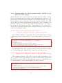
baypass -npop 18 -gfile geno.bta14 -efile bta.pc1 \
-omegafile omega.bta -outprefix anacovis2
The resulting Importance Sampling estimates of the Bayes Factor, the
empirical Bayesian P-value and the underlying regression coefficient 9 might
be plotted as follows:
covis2.snp.res=read.table("anacovis2_summary_betai_reg.out",h=T)
graphics.off()
layout(matrix(1:3,3,1))
plot(covis2.snp.res$BF.dB.,xlab="SNP",ylab="BFis (in dB)")
plot(covis2.snp.res$eBPis,xlab="SNP",ylab="eBPis")
plot(covis2.snp.res$Beta_is,xlab="SNP",ylab=expression(beta~"coefficient"))
5.1.3
Analysis under the MCMC covariate mode: MCMC is run
under the STD model
This analysis allows to perform association study under the STD covariate
model by estimating the empirical Bayesian P-value and the underlying regression coefficient using parameters values sampled from MCMC run under
the STD model (Gautier, 2015). Although one may also estimate Ω under
the STD model, this option has been inactivated in BayPass. As a consequence, an estimate of Ω (e.g., as obtained by a first analysis under the core
model of IS covariate mode) must be provided. The example below corresponds to an association analysis with the SMS covariable measured on the
18 French cattle breeds (Gautier, 2015).
baypass -npop 18 -gfile geno.bta14 -efile bta.pc1 \
-covmcmc -omegafile omega.bta -outprefix anacovmcmc
The resulting estimates of the empirical Bayesian P-values, the underlying regression coefficients (posterior mean) and the corrected XtX might be
plotted as follows:
covmcmc.snp.res=read.table("anacovmcmc_summary_betai.out",h=T)
covmcmc.snp.xtx=read.table("anacovmcmc_summary_pi_xtx.out",h=T)$M_XtX
graphics.off()
layout(matrix(1:3,3,1))
plot(covmcmc.snp.res$eBPmc,xlab="SNP",ylab="eBPmc")
plot(covmcmc.snp.res$M_Beta,xlab="SNP",ylab=expression(beta~"coefficient"))
plot(covmcmc.snp.xtx,xlab="SNP",ylab="XtX corrected for SMS")
9
Note that one may carry out a calibration of these different measures (as detailed for
the XtX in 5.1.1) by analysing a POD together with the covariables:
baypass -npop 18 -gfile G.pods -efile bta.pc1 -omegafile omega.bta -outprefix podcovis
34
5.1.4
Analysis under the AUX covariate mode: MCMC is run
under the AUX model
This analysis allows to perform association study under the AUX covariate
model by estimating the Bayes Factor (and the underlying regression coefficient) using parameters values sampled from MCMC run under the AUX
model (Gautier, 2015). Although one may also estimate Ω under the AUX
model, this option has been inactivated in BayPass. As a consequence, an
estimate of Ω (e.g., as obtained by a first analysis under the core model of
IS covariate mode) must be provided. The example below corresponds to
an association analysis with the SMS covariable measured on the 18 French
cattle breeds (Gautier, 2015).
baypass -npop 18 -gfile geno.bta14 -efile bta.pc1 \
-auxmodel -omegafile omega.bta -outprefix anacovaux
The resulting estimates of the Bayes Factor, the underlying regression
coefficients (posterior mean) and the corrected XtX might be plotted as follows:
covaux.snp.res=read.table("anacovaux_summary_betai.out",h=T)
covaux.snp.xtx=read.table("anacovaux_summary_pi_xtx.out",h=T)$M_XtX
graphics.off()
layout(matrix(1:3,3,1))
plot(covaux.snp.res$BF.dB.,xlab="SNP",ylab="BFmc (in dB)")
plot(covaux.snp.res$M_Beta,xlab="SNP",ylab=expression(beta~"coefficient"))
plot(covaux.snp.xtx,xlab="SNP",ylab="XtX corrected for SMS")
One may further introduce spatial dependency among the SNPs by setting
isβ = 1 in the Ising prior (Figure 1C) to refine the associated region:
baypass -npop 18 -gfile geno.bta14 -efile bta.pc1 -auxmodel \
-isingbeta 1.0 -omegafile omega.bta -outprefix anacovauxisb1
The resulting estimates of the posterior mean of the each auxiliary variable δi under both models (AUX model with no SNP spatial dependency
and AUX model Bayes Factor, the underlying regression coefficients (posterior mean) and the corrected XtX might be plotted as follows:
covauxisb1.snp.res=read.table("anacovauxisb1_summary_betai.out",h=T)
graphics.off()
layout(matrix(1:2,2,1))
plot(covaux.snp.res$M_Delta,xlab="SNP",ylab=expression(delta[i]),main="AUX model")
plot(covauxisb1.snp.res$M_Delta,xlab="SNP",ylab=expression(delta[i]),
main="AUX model with isb=1")
35
5.2
Littorina Pool–Seq read count data
The Littorina Pool–Seq data may be analysed in a similar fashion as the
cattle data above except that one needs to specify the (haploid pool) size file
using the -poolsizefile option to activate the Pool–Seq mode. Because
the haploid pool sizes are relatively large (= 100) in the example, one may
also increase the initial δ of the yij proposal distribution (as a rule of thumbs,
one may set it to a fifth of the minimum pool size). Here is an example of
command to run BayPass under the IS covariate mode (MCMC run under
the core model)10 :
../bin/i_baypass -npop 12 -gfile lsa.geno -efile lsa.ecotype \
-poolsizefile lsa.poolsize -d0yij 20 -outprefix lsacovis
6
Copyright
BayPass is free software under the GNU General Public License (see http:
c INRA.
//www.gnu.org/licenses/gpl-3.0.en.html), and 7
Contact
If you have any question, please feel free to contact me. However, I strongly
recommend you read carefully this manual first.
10
This analysis takes about 12 min with the i_baypass binary
36
Bibliography
Coop, G., D. Witonsky, A. D. Rienzo, and J. K. Pritchard, 2010 Using environmental correlations to identify loci underlying local adaptation. Genetics 185: 1411–1423.
Duforet-Frebourg, N., E. Bazin, and M. G. B. Blum, 2014 Genome scans for
detecting footprints of local adaptation using a bayesian factor model. Mol
Biol Evol 31: 2483–2495.
F¨orstner, W., and B. Moonen, 2003 A metric for covariance matrices. In
Geodesy-The Challenge of the 3rd Millennium. Springer Berlin Heidelberg,
299–309.
Gautier, M., 2015 Genome-wide scan for adaptive divergence and
association with population-specific covariates.
bioRxiv doi:
http://dx.doi.org/10.1101/023721.
Genz, A., F. Bretz, T. Miwa, X. Mi, F. Leisch, et al., 2015 mvtnorm: Multivariate Normal and t Distributions. R package version 1.0-3.
G¨
unther, T., and G. Coop, 2013 Robust identification of local adaptation
from allele frequencies. Genetics 195: 205–220.
Hasselman, B., 2015 geigen: Calculate Generalized Eigenvalues of a Matrix
Pair . R package 1.5.
Nicholson, G., A. V. Smith, F. Jonsson, O. Gustafsson, K. Stefansson,
et al., 2002 Assessing population differentiation and isolation from singlenucleotide polymorphism data. J Roy Stat Soc B 64: 695–715.
Paradis, E., J. Claude, and K. Strimmer, 2004 Ape: Analyses of phylogenetics
and evolution in r language. Bioinformatics 20: 289–290.
Pickrell, J. K., and J. K. Pritchard, 2012 Inference of population splits
and mixtures from genome-wide allele frequency data. PLoS Genet 8:
e1002967.
R Core Team, 2015 R: A Language and Environment for Statistical Computing. R Foundation for Statistical Computing, Vienna, Austria.
Riebler, A., L. Held, and W. Stephan, 2008 Bayesian variable selection for
detecting adaptive genomic differences among populations. Genetics 178:
1817–1829.
37
Spiegelhalter, D. J., N. G. Best, B. P. Carlin, and A. v. d. Linde, 2002
Bayesian measures of model complexity and fit. Journal of the Royal
Statistical Society. Series B (Statistical Methodology) 64: 583–639.
Wei, T., 2013 corrplot: Visualization of a correlation matrix . R package
version 0.73.
Westram, A. M., J. Galindo, M. A. Rosenblad, J. W. Grahame, M. Panova,
et al., 2014 Do the same genes underlie parallel phenotypic divergence in
different littorina saxatilis populations? Mol Ecol 23: 4603–4616.
38