Download Phycas User Manual - Holder Lab Web page

Phycas User Manual
Version 1.2.0
Paul O. Lewis, Mark. T. Holder, and David L. Swofford
August 2, 2010
Contents
1 Introduction
1.1
4
What’s new in version 1.2? . . . . . . . . . . . . . . . . . . . . . . . . . . . . . . . . . . . . .
4
Bugs fixed . . . . . . . . . . . . . . . . . . . . . . . . . . . . . . . . . . . . . . . . . . . . . . .
4
1.2
What’s new in version 1.1.x? . . . . . . . . . . . . . . . . . . . . . . . . . . . . . . . . . . . .
4
1.3
What’s new in version 1.1? . . . . . . . . . . . . . . . . . . . . . . . . . . . . . . . . . . . . .
4
New features . . . . . . . . . . . . . . . . . . . . . . . . . . . . . . . . . . . . . . . . . . . . .
4
Bugs fixed . . . . . . . . . . . . . . . . . . . . . . . . . . . . . . . . . . . . . . . . . . . . . . .
5
How to use this manual . . . . . . . . . . . . . . . . . . . . . . . . . . . . . . . . . . . . . . .
5
1.4
2 Features
5
2.1
Slice sampling . . . . . . . . . . . . . . . . . . . . . . . . . . . . . . . . . . . . . . . . . . . . .
5
2.2
Hierarchical models . . . . . . . . . . . . . . . . . . . . . . . . . . . . . . . . . . . . . . . . . .
6
2.3
Polytomy priors . . . . . . . . . . . . . . . . . . . . . . . . . . . . . . . . . . . . . . . . . . . .
6
2.4
Marginal Likelihoods . . . . . . . . . . . . . . . . . . . . . . . . . . . . . . . . . . . . . . . . .
7
2.5
Conditional Predictive Ordinates . . . . . . . . . . . . . . . . . . . . . . . . . . . . . . . . . .
8
3 Tutorial
3.1
3.2
8
Warming up to Phycas . . . . . . . . . . . . . . . . . . . . . . . . . . . . . . . . . . . . . . . .
8
First things first . . . . . . . . . . . . . . . . . . . . . . . . . . . . . . . . . . . . . . . . . . .
9
Starting from a terminal on Windows . . . . . . . . . . . . . . . . . . . . . . . . . . . . . . .
9
Starting from the Phycas.app bundle under MacOS . . . . . . . . . . . . . . . . . . . . . . . .
9
Getting help . . . . . . . . . . . . . . . . . . . . . . . . . . . . . . . . . . . . . . . . . . . . . .
9
A basic analysis . . . . . . . . . . . . . . . . . . . . . . . . . . . . . . . . . . . . . . . . . . . .
12
Before proceeding...
. . . . . . . . . . . . . . . . . . . . . . . . . . . . . . . . . . . . . . . . .
12
The basic.py script . . . . . . . . . . . . . . . . . . . . . . . . . . . . . . . . . . . . . . . . . .
12
Line-by-line explanation . . . . . . . . . . . . . . . . . . . . . . . . . . . . . . . . . . . . . . .
13
Invoking phycas commands . . . . . . . . . . . . . . . . . . . . . . . . . . . . . . . . . . . . .
15
1
Running basic.py . . . . . . . . . . . . . . . . . . . . . . . . . . . . . . . . . . . . . . . . . . .
3.3
3.4
3.5
3.6
Output of basic.py . . . . . . . . . . . . . . . . . . . . . . . . . . . . . . . . . . . . . . . . . .
16
Summarizing tree files . . . . . . . . . . . . . . . . . . . . . . . . . . . . . . . . . . . . . . . .
16
The summarize.py script . . . . . . . . . . . . . . . . . . . . . . . . . . . . . . . . . . . . . . .
16
Line-by-line explanation . . . . . . . . . . . . . . . . . . . . . . . . . . . . . . . . . . . . . . .
17
Running summarize.py . . . . . . . . . . . . . . . . . . . . . . . . . . . . . . . . . . . . . . . .
18
Output of summarize.py . . . . . . . . . . . . . . . . . . . . . . . . . . . . . . . . . . . . . . .
18
Defining a partition model . . . . . . . . . . . . . . . . . . . . . . . . . . . . . . . . . . . . . .
19
The partition.py script . . . . . . . . . . . . . . . . . . . . . . . . . . . . . . . . . . . . . . . .
19
Running partition.py . . . . . . . . . . . . . . . . . . . . . . . . . . . . . . . . . . . . . . . . .
20
Line-by-line explanation . . . . . . . . . . . . . . . . . . . . . . . . . . . . . . . . . . . . . . .
20
Output of partition.py . . . . . . . . . . . . . . . . . . . . . . . . . . . . . . . . . . . . . . . .
22
Estimating marginal likelihoods . . . . . . . . . . . . . . . . . . . . . . . . . . . . . . . . . . .
23
The steppingstone.py script . . . . . . . . . . . . . . . . . . . . . . . . . . . . . . . . . . . . .
24
Running steppingstone.py . . . . . . . . . . . . . . . . . . . . . . . . . . . . . . . . . . . . . .
25
Line-by-line explanation . . . . . . . . . . . . . . . . . . . . . . . . . . . . . . . . . . . . . . .
25
Output of steppingstone.py . . . . . . . . . . . . . . . . . . . . . . . . . . . . . . . . . . . . .
27
Polytomy analyses . . . . . . . . . . . . . . . . . . . . . . . . . . . . . . . . . . . . . . . . . .
28
Exploring the polytomy prior . . . . . . . . . . . . . . . . . . . . . . . . . . . . . . . . . . . .
29
The polytomy.py script . . . . . . . . . . . . . . . . . . . . . . . . . . . . . . . . . . . . . . . .
29
Line-by-line explanation . . . . . . . . . . . . . . . . . . . . . . . . . . . . . . . . . . . . . . .
30
4 Reference
4.1
4.2
16
32
Probability Distributions . . . . . . . . . . . . . . . . . . . . . . . . . . . . . . . . . . . . . . .
32
Terminology . . . . . . . . . . . . . . . . . . . . . . . . . . . . . . . . . . . . . . . . . . . . . .
32
Using probability distributions in Phycas . . . . . . . . . . . . . . . . . . . . . . . . . . . . .
32
Probability distributions available in Phycas . . . . . . . . . . . . . . . . . . . . . . . . . . . .
34
Bernoulli
. . . . . . . . . . . . . . . . . . . . . . . . . . . . . . . . . . . . . . . . . . . . . . .
34
Beta . . . . . . . . . . . . . . . . . . . . . . . . . . . . . . . . . . . . . . . . . . . . . . . . . .
34
BetaPrime . . . . . . . . . . . . . . . . . . . . . . . . . . . . . . . . . . . . . . . . . . . . . . .
35
Binomial . . . . . . . . . . . . . . . . . . . . . . . . . . . . . . . . . . . . . . . . . . . . . . . .
35
Dirichlet . . . . . . . . . . . . . . . . . . . . . . . . . . . . . . . . . . . . . . . . . . . . . . . .
36
Exponential . . . . . . . . . . . . . . . . . . . . . . . . . . . . . . . . . . . . . . . . . . . . . .
36
Gamma . . . . . . . . . . . . . . . . . . . . . . . . . . . . . . . . . . . . . . . . . . . . . . . .
37
InverseGamma . . . . . . . . . . . . . . . . . . . . . . . . . . . . . . . . . . . . . . . . . . . .
37
Lognormal . . . . . . . . . . . . . . . . . . . . . . . . . . . . . . . . . . . . . . . . . . . . . . .
37
Normal . . . . . . . . . . . . . . . . . . . . . . . . . . . . . . . . . . . . . . . . . . . . . . . .
38
RelativeRate . . . . . . . . . . . . . . . . . . . . . . . . . . . . . . . . . . . . . . . . . . . . .
38
2
Uniform . . . . . . . . . . . . . . . . . . . . . . . . . . . . . . . . . . . . . . . . . . . . . . . .
39
Models . . . . . . . . . . . . . . . . . . . . . . . . . . . . . . . . . . . . . . . . . . . . . . . . .
39
JC . . . . . . . . . . . . . . . . . . . . . . . . . . . . . . . . . . . . . . . . . . . . . . . . . . .
40
F81
. . . . . . . . . . . . . . . . . . . . . . . . . . . . . . . . . . . . . . . . . . . . . . . . . .
40
K80 . . . . . . . . . . . . . . . . . . . . . . . . . . . . . . . . . . . . . . . . . . . . . . . . . .
40
HKY . . . . . . . . . . . . . . . . . . . . . . . . . . . . . . . . . . . . . . . . . . . . . . . . . .
41
GTR . . . . . . . . . . . . . . . . . . . . . . . . . . . . . . . . . . . . . . . . . . . . . . . . . .
41
Proportion of invariable-sites . . . . . . . . . . . . . . . . . . . . . . . . . . . . . . . . . . . .
41
Discrete gamma . . . . . . . . . . . . . . . . . . . . . . . . . . . . . . . . . . . . . . . . . . . .
42
4.4
Settings . . . . . . . . . . . . . . . . . . . . . . . . . . . . . . . . . . . . . . . . . . . . . . . .
42
4.5
Settings used by like . . . . . . . . . . . . . . . . . . . . . . . . . . . . . . . . . . . . . . . .
42
4.6
Settings used by mcmc . . . . . . . . . . . . . . . . . . . . . . . . . . . . . . . . . . . . . . . .
42
4.7
Settings used by model . . . . . . . . . . . . . . . . . . . . . . . . . . . . . . . . . . . . . . .
46
4.8
Settings used by randomtree . . . . . . . . . . . . . . . . . . . . . . . . . . . . . . . . . . .
48
4.9
Settings used by ss . . . . . . . . . . . . . . . . . . . . . . . . . . . . . . . . . . . . . . . . .
49
4.10 Settings used by sump . . . . . . . . . . . . . . . . . . . . . . . . . . . . . . . . . . . . . . . .
49
4.11 Settings used by sumt . . . . . . . . . . . . . . . . . . . . . . . . . . . . . . . . . . . . . . . .
50
4.3
5 Design principles
51
5.1
Why was Phycas written as an extension to Python? . . . . . . . . . . . . . . . . . . . . . . .
51
5.2
Why is there no graphical user interface (GUI)? . . . . . . . . . . . . . . . . . . . . . . . . . .
52
5.3
Is Phycas slower than MrBayes? . . . . . . . . . . . . . . . . . . . . . . . . . . . . . . . . . .
52
6 Installing Phycas
6.1
52
TM
Instructions for Windows
Windows
TM
users . . . . . . . . . . . . . . . . . . . . . . . . . . . . . . . . . .
52
console . . . . . . . . . . . . . . . . . . . . . . . . . . . . . . . . . . . . . . . . . .
53
TM
. . . . . . . . . . . . . . . . . . . . . . . . . . . . . . . .
53
TM
. . . . . . . . . . . . . . . . . . . . . . . . . . . . . . . .
53
Installing Python under Windows
Installing Phycas under Windows
TM
Locating the “Phycas Installation Folder” under Windows
6.2
. . . . . . . . . . . . . . . . . .
54
Instructions for MacIntosh Users . . . . . . . . . . . . . . . . . . . . . . . . . . . . . . . . . .
54
The iTerm terminal application . . . . . . . . . . . . . . . . . . . . . . . . . . . . . . . . . . .
54
Installing Python on a Mac . . . . . . . . . . . . . . . . . . . . . . . . . . . . . . . . . . . . .
54
Installing Phycas on a Mac . . . . . . . . . . . . . . . . . . . . . . . . . . . . . . . . . . . . .
54
Locating the “Phycas Installation Folder” on a Mac . . . . . . . . . . . . . . . . . . . . . . .
54
References
56
3
1
Introduction
Phycas (http://www.phycas.org) is an extension of the Python programming language (http://www.
python.org) that allows Python to read NEXUS-formatted data files, run Bayesian phylogenetic MCMC
analyses, and summarize the results. In order to use Phycas, you need to first have Python installed on your
computer. Please see section 6 entitled “Installing Phycas” (p. 52) for detailed installation instructions and
useful information on topics important for using Phycas, such as how to obtain a command prompt for the
operating system you are using. The following sections assume that you have successfully installed Phycas
and have read section 6.
1.1
What’s new in version 1.2?
This version was released on 20 July 20101 . It adds support for data partitioning, changes the name of the
ps command to ss, and adds the cpo command. Phycas now supports a limited form of data partitioning
in that topology and edge lengths are always linked across partition subsets and all other model parameters
are unlinked. The name change from ps to ss reflects the fact that the primary purpose of the command is
to use the Stepping Stone method, and “ps” stands for “path sampling,” a name that was never used even
by the authors of the thermodynamic integration approach! Finally, the cpo command is identical to the
mcmc command except that it saves the site log-likelihoods to a file and estimates the Conditional Predictive
Ordinate for each site using those stored site log-likelihoods. See section 2.5 for details.
The process of specifying a master pseudorandom number seed has been simplified in version 1.2. You
can now simply insert the command setMasterSeed(13579) just after the from phycas import *
command to set the master random number seed to the value 13579.
Bugs fixed
The BUGS file documents two additional bug fixes prior to this release. They are the “underflow” bug
(brought to our attention by Federico Plazzi and Mark Clements), which resulted in incorrect likelihood
calculations for large trees when a “+I” model was in use, and the “Jockusch” bug (brought to our attention
by Elizabeth Jockusch), which resulted in “not-a-number” likelihoods when a particular subset relative rate
was very tiny.
1.2
What’s new in version 1.1.x?
These are bug-fix releases. For a description of the major bug fixed, see the section on the “underflow” bug
in the BUGS file. For other changes, see the CHANGES file.
1.3
What’s new in version 1.1?
New features
The ps and sump commands are new to version 1.1. The ps command allows computation of both the path
sampling (a.k.a. thermodynamic integration) method of Lartillot and Phillippe (2006) and the steppingstone
sampling method introduced by Xie et al. (2010). See section 2.4 on page 7 for details. The sump command
provides an analog of the sump command in MrBayes, providing means, extremes, and credible intervals for
model parameters based on samples saved in the parameter file.
1 This
version corresponds with git commit SHA 18e7a835616e453dcfd60d1b9ee9e763858778cc
4
Bugs fixed
Two memory leaks were fixed prior to this release. For a description of the leaks and what was done to fix
them, see the section on the “leaky” bug in the BUGS file.
1.4
How to use this manual
This manual begins with a description of some things you can do with Phycas that you cannot do with most
other Bayesian phylogenetics software. Following this features section (section 2) is a tutorial (section 3)
showing you how to perform some simple analyses. This tutorial does not attempt to explain all possible
settings. The online help system provides details about settings not mentioned in the tutorial. After
these initial sections, the manual switches to reference style (section 4), detailing probability distributions
(sections 4.1 and 4.2) that can be used as priors, and describing the models of character evolution (section 4.3)
available in Phycas. Toward the end you will find an annotated listing (section 4.4) of Phycas settings. This
is followed by a discussion (section 5) of design principles (e.g. Why did we decide to extend Python rather
than write a stand-alone program? Why is there no graphical interface?). The final section (section 6) is
devoted to the details of getting Phycas (and Python) installed on your computer system.
2
Features
Phycas differs in some ways from other programs that conduct Bayesian phylogenetic analyses. The following
sections are meant to highlight some of the features present in Phycas that are uncommon or absent in other
programs.
2.1
Slice sampling
Phycas makes extensive use of an MCMC method known as slice sampling (Neal, 2003), whereas many
programs use Metropolis-Hastings (MH) proposals to update model parameters during an MCMC analysis.
The decision to use slice sampling in Phycas was based on the fact that the efficiency of slice samplers can be
tuned as they run. In contrast, MH depends on tuning parameters that must be adjusted prior to sampling,
an activity almost never performed in practice, leading to inefficient MCMC sampling for data sets that are
not like those used when decisions were being made about default values of tuning parameters. In the final
tally, a program using slice sampling behaves nearly identically to one using MH if the program using MH
has been tuned prior to the analysis; however, Phycas saves you from having to worry about tuning by doing
it automatically during the run.
Phycas first attempts to adapt its slice samplers (one slice sampler is assigned to each model parameter)
at the cycle specified by the setting mcmc.adapt first. Each subsequent adaptation occurs after twice as
many cycles as the previous adaptation. After the first few adaptations there is usually little to be gained
by adapting the slice samplers further, hence the increasingly long time periods between adaptations.
Slice sampling can be used only for continuous model parameters, not for updating the tree topology. Phycas
uses the Larget and Simon (1999) “LOCAL move without a molecular clock” to propose simultaneous changes
in tree topology and edge lengths. Because edge length parameters are closely tied to the topology (and
because there are so many of them!), it appears to be more efficient to use the LOCAL move rather than
slice samplers to update edge lengths.
5
2.2
Hierarchical models
It is common still in Bayesian phylogenetics to use non-hierarchical models. In a non-hierarchical model,
all parameters in the model can be found in the likelihood function. Edge lengths are parameters found
in the likelihood function and, typically, a single Exponential distribution is used as the prior distribution
for all edge lengths. The problem with this is that the edge length prior often has more of an effect than
intended (the average tree length often responds to changes in the edge length prior mean) and researchers
are often at a loss when deciding on an appropriate prior mean for edge lengths. It is possible to take an
empirical Bayes approach, which involves estimating edge lengths under maximum likelihood and using the
average estimated edge length as the mean of the prior. Bayesian purists eschew peeking at the data to help
determine the prior, but how should one choose an appropriate prior distribution without using estimates?
Phycas provides for the use of hierarchical models to solve this problem in a purely Bayesian way. In a
hierarchical model, some parameters (called hyperparameters) are not found in the likelihood function.
They are in this sense one level removed from the data, hence the use of the term “hierarchical.” In the
case of edge lengths, Phycas can use a hyperparameter to determine the mean of the edge length prior
distribution, taking this responsibility away from the researcher, who is relieved to learn that she now
only needs to specify the parameters of the hyperprior — the prior distribution of the hyperparameter.
Because hyperparameters are one level (or more) removed from the data, the effects of arbitrary choices
in the specification of the hyperprior is much less pronounced. In fact, just letting Phycas use its default
hyperprior works well because it is vague enough that the hyperprior (determining edge length prior means)
will begin to hover around a value appropriate for the data at hand. The effect is similar to the empirical
Bayes approach, but you need not compromise your Bayesian principles and, rather than fixing the mean of
the edge length prior, you are effectively estimating it as the MCMC analysis progresses.
To tell Phycas to use a hierarchical model for edge lengths, you need only set mcmc.using hyperprior to
True. The hyperprior distribution is determined by the setting mcmc.edgelen hyperprior.
2.3
Polytomy priors
A solution to the “Star Tree Paradox” problem was proposed by Lewis, Holder, and Holsinger (2005). Their
solution was to use reversible-jump MCMC to allow unresolved tree topologies to be sampled during the
course of a Bayesian phylogenetic analysis in addition to fully-resolved tree topologies. If the time between
speciation events is so short (or the substitution rate so low) that no substitutions occurred along a particular
internal edge in the true tree, then use of the polytomy prior proposed by Lewis, Holder, and Holsinger
(2005) can improve inference by giving the Bayesian model a “way out.” That is, it is not required to find
a fully resolved tree, but is allowed to place a lot of posterior probability mass on a less-than-fully-resolved
topology. Please refer to the Lewis, Holder, and Holsinger (2005) paper for details.
To use the polytomy prior in an analysis, be sure that mcmc.allow polytomies and mcmc.polytomy prior
are both True. The setting mcmc.topo prior C determines the strength of the polytomy prior. Setting
mcmc.topo prior C to 1.0 results in a flat prior (all topologies have identical prior probabilities, and thus
unresolved topologies get no more or less weight than fully-resolved topologies). Setting mcmc.topo prior C
greater than 1.0 favors less resolved topologies more than fully-resolved ones. This is usually what is desired;
even with a prior that favors unresolved trees, a fully-resolved topology can easily win out over a less-resolved
one if there is even scant evidence for substitution along the relevant edge. In the paper, this value was set
to the value e (the base of the natural logarithms). To do this in Phycas, set mcmc.topo prior C equal
math.exp(1.0).
The example <phycas install directory>/phycas/Examples/Paradox/Paradox.py shows a complete example
of an analysis using the polytomy prior. If executed, this example script will recreate the analysis presented
in Figure 4 of the Lewis, Holder, and Holsinger (2005) paper. Also, a section (3.6) of the tutorial covers
6
polytomy analyses.
2.4
Marginal Likelihoods
Phycas offers several ways of estimating marginal (model) likelihoods. The marginal likelihood represents
the average fit of the model to the data (as measured by the likelihood), where the average is a weighted
average over all parameter values, the weights being provided by the joint prior distribution. If you initiate
an MCMC analysis using the mcmc command, Phycas reports the marginal likelihood using the well-known
harmonic mean method introduced by Newton and Raftery (1994). The harmonic mean method is widely
known to overestimate the marginal likelihood, not penalizing models enough for having extra parameters
that do not substantially increase the overall fit of the model. In addition, the variance of the harmonic
mean estimator can be infinite, making this estimator potentially very unreliable.
Phycas can use two alternatives to the harmonic mean method — thermodynamic integration (Lartillot and
Phillippe, 2006) (also known as path sampling), and the stepping stone method (Xie et al., 2010; Fan et al.,
2010) — but only if the MCMC analysis is conducted using the ss command. The thermodynamic integration
(TI) and stepping stone (SS) methods both require running a special MCMC analysis that explores a series
of power posterior distributions. The power posterior is proportional to L(θ)β p(θ)β π(θ)1−β , where L(θ) is
the likelihood, p(θ) is the prior, π(θ) is a “reference distribution” and β is the power.
The value of β is slowly decreased from 1 (in which MCMC is exploring the posterior distribution) to 0
(in which MCMC is exploring the reference distribution) in small steps. The number of β values used is
specified by ss.nbetavals.2 When the command ss is invoked, an MCMC analysis is run for each of the
ss.nbetavals values of β. The current settings of the mcmc command are used for each value of β; however,
the mcmc.burnin setting governs only the initial burn-in period (i.e. there is no separate burnin between
successive values of β). At the end of the run, Phycas will report the log of the marginal likelihood estimated
using the SS method.
The ss.ti option controls whether or not the stepping-stone command uses thermodynamic integration. By
default, the ss.ti is False estimates the marginal likelihood using the version of the SS method described
by Fan et al. (2010). In this version of SS, the reference distribution is a parameterized version of the
posterior distribution. The first portion of the analysis gathers samples from the posterior distribution. The
mean and variance of each parameter are estimated from this posterior sample. These summary statistics
are used to create a reference distribution that approximates the posterior. For a simple example, if a model
has two parameters and a Normal prior was associated with each parameter, then the reference distribution
would be an uncorrelated bivariate Normal distribution in which the marginal means and variances equal
the sample means and variances of the two parameters from the initial posterior sample.
In thermodynamic integration (ss.ti = True) the reference distribution, π(θ), is simply the prior, p(θ).
The prior is also used as reference distribution in the version of the stepping stone described by Xie et al.
(2010). When ss.ti = True, Phycas will provide marginal likelihood estimates for TI and the Xie et al.
(2010) version of stepping stone. Xie et al. (2010) found that choosing β values that are not equally spaced
along the path from 1 to 0 substantially improves the efficiency of both TI and this version of SS. Phycas uses
evenly-spaced quantiles of a Beta(a,b) distribution to choose β values, where the two shape parameters of the
Beta distribution, a and b, are specified as ss.shape1 and ss.shape2, respectively. By default, ss.shape1
and ss.shape2 are both set to 1.0, but when ss.ti is set to True, you should also change ss.shape1 to
a small value such as 0.3 (leaving ss.shape2 equal to 1.0).
The example <phycas install directory>/phycas/Examples/Steppingstone/Steppingstone.py shows a complete example of the use of path/steppingstone sampling for marginal likelihood estimation. This example
2 You can change the minimum and maximum β values are set using ss.minbeta and ss.maxbeta (it is best to leave
these set to their default values of 0 and 1, respectively)
7
recreates part of Figure 10 in the Xie et al. (2010) paper. Also, one section of the tutorial (3.5) covers
marginal likelihood estimation.
2.5
Conditional Predictive Ordinates
Conditional predictive ordinates (CPO) provide a way to assess the fit of the model to each site individually,
much like the analysis of residuals in a regression analysis. The CPO for site i equals p(yi |y(i) ), where yi
represents the data for site i and y((i) represents all data except that for site i. CPOs are thus a form of
cross-validation in which the predictive distribution from all data except that from site i is used to predict
the data observed at site i. The CPO for site i is a measure of the success of the prediction, with high values
meaning the data for site i can be accurately predicted by a model based on all other data, and low values
meaning that predictions made from a model trained on all other data would often fail to correctly predict
the data at the focal site. Note that Phycas reports CPO values on the log scale, and thus these values are
always negative (a log(CPO) equal to 0.0 would be equivalent to a probability of 1.0, which would be seen
only for a tree in which all edge lengths are zero).
To get Phycas to calculate CPO values, specify True for mcmc.save sitelikes. This will cause Phycas
to save a (sometimes very large) “sitelikes” file containing the site log-likelihoods for every site for every
sample. Thus, if your alignment comprises 2000 sites and you specify mcmc.ncycles to be 10000 and
mcmc.sample every to be 10, then this file will contain 1000 rows and 2000 columns. The name of the file
produced can be specified with mcmc.out.sitelikes setting (the file will be named sitelikes.txt by
default). You must used the command sump to summarize this file after the analysis is finished. Set the
option sump.cpofile equal to a string specifying the name of the file of site likelihoods produced by the
mcmc command. You must specify sump.cpofile even if you did not modify mcmc.out.sitelikes because,
by default, the sump command does not even look for a file of site likelihoods to summarize. In its summary,
the sump command will use the harmonic mean of the site likelihoods in one column of the sitelikes file as the
estimate of the CPO for the site represented by that column. (If you calculate these in some other program,
such as Excel, note that the estimator equals the log of the harmonic mean of the sampled site likelihoods,
not the harmonic mean of the sampled site log-likelihoods.) While the harmonic mean method is unstable
for estimating the overall marginal likelihood, it provides a stable and accurate method for estimating CPO
values. The sump command will not only output the overall log CPO (calculated as the sum over sites of the
log CPO at each site), but will generate a file containing the commands for generating a plot of log(CPO)
vs. site in the software R (http://www.r-project.org/).
3
3.1
Tutorial
Warming up to Phycas
Phycas is an extension of Python, so to use it you must first start Python. In this section, you will learn
how to invoke Phycas commands from the Python command line. After you become familiar with the basic
commands, you will probably want to create a file containing the Phycas commands for a particular analysis.
Creating such a file (a Python script) makes it easier to remember exactly what analyses you performed at
some later time. If you want to redo an analysis, having the commands in a script file means you do not
have to type the majority of the commands over again. We will switch to using scripts in section 3.2 (“A
basic analysis”).
8
First things first
The way Phycas is run depends on the operating system you are using. If you are using the Windows
or Linux versions, you start Phycas by opening a terminal (in Windows this is referred to as a “console
window” or “command prompt”) and typing python to invoke Python. If you are using a Mac, you will have
downloaded the Phycas.app bundle that is built around the open-source terminal program iTerm (http:
//iterm.sourceforge.net/). Starting Phycas.app by double-clicking the Phycas icon automatically
starts an iTerm terminal, invokes Python, and loads Phycas.
Starting from a terminal on Windows
To start Python on Windows, open a console window (a.k.a. terminal window) and type the word python.
This should generate output similar to the following:
Python 2.5.1 (r251:54863, Oct 30 2007, 13:54:11)
[GCC 4.1.2 20070925 (Red Hat 4.1.2-33)] on linux2
Type "help", "copyright", "credits" or "license" for more information.
>>>
At the >>> prompt, type from phycas import *, like this:
>>> from phycas import *
>>>
Phycas is an “extension” of Python, but you must import extensions in order for their capabilities to be
available. The import statement you typed means “import everything phycas has to offer.”
Starting from the Phycas.app bundle under MacOS
If you are using the Phycas.app bundle on MacOS, you can launch the Phycas application
by double clicking on the icon. Although the name appears to be just Phycas, it is really
Phycas.app; the MacOS hides the .app extension unless you change this in the Finder preferences. (We will hereafter use the terms Phycas application and Phycas.app bundle
interchangeably.) The Phycas application will show up in your dock and the window that
appears will be a terminal that has already invoked Python and issued the from phycas
import * command mentioned in many places in this manual.
All the instructions for the rest of the manual will be executed the same way regardless of whether Phycas
running from a Windows console window, a Linux terminal or the Phycas application.
Getting help
Now type help at the Python prompt. This will display the following help message:
>>> help
Phycas Help
For Python Help use "python_help()"
Commands are invoked by following the name by () and then
hitting the RETURN key. Thus, to invoke the sumt command use:
9
sumt()
Commands (and almost everything else in python) are case-sensitive -- so
"Sumt" is _not_ the same thing as "sumt" In general, you should use the
lower case versions of the phycas command names.
The currently implemented Phycas commands are:
like
mcmc
model
randomtree
ss
sump
sumt
Use <command_name>.help to see the detailed help for each command. So,
sumt.help
will display the help information for the sumt command object.
Ordinarily, typing help will invoke the Python help system; however, note that after Phycas has been
imported into Python, typing help now invokes the Phycas help system. You can still access Python’s
interactive help by typing python help()3 . Hopefully, the output is self-explanatory, so let’s try what the
output of the help command suggests: obtaining help for a particular command. Type model.help at the
Python prompt (>>>):
>>> model.help
model
Defines a substitution model.
Available input options:
Attribute
Explanation
============================== =================================================
type
Can be 'jc', 'hky', 'gtr' or 'codon'
update_relrates_separately
If True, GTR relative rates will be individually
updated using slice sampling; if False, they will
be updated jointly using a Metropolis-Hastings
move (generally both faster and better).
relrate_prior
The joint prior distribution for all six GTR
relative rate parameters. Used only if
update_relrates_separately is False.
relrate_param_prior
The prior distribution for individual GTR
relative rate parameters. Used only if
update_relrates_separately is true.
relrates
The current values for GTR relative rates. These
should be specified in this order: A<->C, A<->G,
A<->T, C<->G, C<->T, G<->T.
3 If
you do try typing python help(), note that you can quit the Python help system (and return to using Phycas) by
typing quit at the help> prompt
10
fix_relrates
...
Current model input settings:
Attribute
==============================
type
update_relrates_separately
relrate_prior
If True, GTR relative rates will not be modified
during the course of an MCMC analysis
Current Value
=================================================
'hky'
True
Dirichlet((1.00000, 1.00000, 1.00000, 1.00000,
1.00000, 1.00000))
Exponential(1.00000)
[1.0, 4.0, 1.0, 1.0, 4.0, 1.0]
False
Exponential(1.00000)
4.0
False
Exponential(20.00000)
0.05
False
1
Exponential(1.00000)
0.5
False
relrate_param_prior
relrates
fix_relrates
kappa_prior
kappa
fix_kappa
omega_prior
omega
fix_omega
num_rates
gamma_shape_prior
gamma_shape
fix_shape
...
fix_edgelens
False
============================== =================================================
>>>
You will probably need to scroll up to see all of the output of the model.help command. Only a portion of
the output has been shown (as indicated by the ellipses). The output shows what model options are available
and, at the end, the current values for those options. Thus, we see that model.type can be one of three
things (’jc’, ’hky’ or ’gtr’) and that the current model type is ’hky’. Suppose you wanted to use the
GTR model rather than the HKY model. You can do this by changing the model.type option as follows:
>>> model.type = 'gtr'
>>> model.current
Entering model.current (or the abbreviated version, model.curr) shows the list of current values, allowing
you to confirm that your change has been made.
The quotes around ’gtr’ are important. They indicate to Python that you are specifying a string (a series
of text characters) rather than the name of some other sort of object. If you typed gtr without the quotes,
Python would assume you are referring to a variable. Because it will (presumably) not find a variable by
that name, you will get the following error message if you forget the quotes:
>>> model.type = gtr
Error: name 'gtr' is not defined
Note that python is forgiving about whether you use double-quotes to delimit strings or single-quotes – either
will work to tell Python that you mean a string rather than the name of a variable. Do not be confused by
the subtle differences in typesetting within this manual. In all cases you should use plain quotes in Python
(not the “back-tick” character or any special curved quote that is found in some word-processing programs).
11
The option model.kappa prior specifies the prior probability distribution to use for the transition/transversion
rate ratio. Phycas defines several probability distributions for use as priors. In this case, the current value
of Exponential(1.00000) indicates that the κ parameter will be assigned an exponential(1) prior distribution. See section 4.2 (p. 34) for a complete list of probability distributions available within Phycas.
The option model.relrates specifies the values of the six GTR relative rates parameters. The square
brackets around the value of the model.relrates parameter, [1.0, 4.0, 1.0, 1.0, 4.0, 1.0],
indicate that you should specify the six relative rate values as a Python list. These should be specified in
this order: A↔C, A↔G, A↔T, C↔G, C↔T, G↔T. The model.relrates option and others like it, such
as model.kappa, model.state freqs, model.gamma shape, and model.pinvar are used to set the starting
values for an MCMC analysis (the mcmc command) or to specify the values of parameters for calculating the
likelihood (the like command).
The model.fix relrates command is used to specify whether the relative rates are to be allowed to vary
during an MCMC analysis (model.fix relrates=False) or are to be frozen at the values specified by
model.relrates (model.fix relrates=True). The values True and False are known to Python and
should not be surrounded by quotes (note also that case is important: typing true or TRUE will generate a
“not defined” error message from Python).
3.2
A basic analysis
The next task is to create a Python script containing the commands to carry out a basic MCMC analysis.
A Python script is a file containing Python source code (including Phycas commands). When submitted to
the Python interpreter (a computer program), the commands in the script file are read and executed.
Before proceeding...
Exit your current Python session by typing Ctrl-d (MacOS or Linux) or Ctrl-z (Windows). If you are using
Phycas.app on MacOS, type Ctrl-d one more time to exit the terminal shell (this will make the iTerm window
disappear).
Create a new, empty directory (a.k.a. folder) in which to experiment. Copy the file green.nex into
the new directory. This file can be found under your Phycas installation directory at the location phycas/Tests/Data/green.nex. If you have no idea where your Phycas installation directory is located, please
refer to the relevant subsection of the installation instructions (either section 6.1 if you are using Windows,
or section 6.2 if you are using a Mac).
The basic.py script
Create a new (plain text4 ) file in the folder (which should contain only the file green.nex). Name the new
file basic.py and type (or copy/paste) the following lines into the file:
from phycas import *
setMasterSeed(98765)
mcmc.data_source = 'green.nex'
4 It is important to save the file using plain text format. Most word processing programs, such as MicrosoftTM WordTM ,
save files by default in a format that contains a lot of extra, proprietary information. All such programs have the option to
save the file as plain text. It is best to create Python scripts using an editor that only saves files as plain text. Examples (for
WindowsTM ) include Notepad++ and Pythonwin (or the simple Notepad program that comes with WindowsTM ). For Macs,
Text Wrangler or BBEdit are good choices. Python comes with its own editor, named Idle, that is also a good (if slightly
sluggish) choice. jEdit (http://www.jedit.org/) is a Java-Based text editor that works well on all platforms.
12
mcmc.out.log = 'basic.log'
mcmc.out.log.mode = REPLACE
mcmc.out.trees.prefix = 'green'
mcmc.out.params.prefix = 'green'
mcmc.ncycles = 2000
mcmc.sample_every = 10
mcmc()
Line-by-line explanation
from phycas import *
N When you first start Python, it knows nothing about Phycas. You must import the functionality provided
by Phycas before any of the Phycas commands described in this manual will work. This first line tells the
Python interpreter to import everything (the asterisk symbol means “everything”) from the phycas module.
This line should start every Phycas script you create.5
setMasterSeed(98765)
N If you were to leave out the line above, you would obtain perfectly valid results, but the output would
be different each time you ran the script. Most of the time you would probably like to have the option of
later repeating an analysis exactly (for example, you might want to make the Phycas script used to obtain
the results for a published paper available to reviewers or the scientific community). To do this in Phycas,
you must use the setMasterSeed command. This command establishes the first in a long sequence of
pseudorandom numbers that Phycas will use for the stochastic aspects of its Markov chain Monte Carlo
analyses.
Pseudorandom numbers (as the name suggests) are not really random, but they behave for all intents and
purposes like random numbers. One difference between the numbers generated by Phycas’ pseudorandom
number generator and real random numbers is that a sequence of pseudorandom numbers is repeatable,
whereas sequences of true random numbers are not repeatable. To repeat a sequence of pseudorandom
numbers, you must start with the same pseudorandom nubmer seed, which should be a positive integer
(whole number). Here we’ve set the seed to the number 98765. Be sure to invoke the setMasterSeed
command just after the from phycas import * command; if you set the master seed after Phycas begins
5 Note that you do not need to type this line if you are using the MacOS version of Phycas (although it doesn’t hurt to enter
from phycas import * again). The MacOS version of Phycas automatically executes this line before presenting you with
the Python prompt.
13
using pseudorandom numbers, then your results will differ from run to run.
mcmc.data_source = 'green.nex'
N This line specifies that the data should be read from the file named green.nex. In our case, green.nex
is in the same directory as this script, but if it were in a different folder then you would need to specify a
relative or absolute path to the file6 . Phycas does not do anything at this point in the script except create
a DataSource object that will read the file ’green.nex’ and make the mcmc.data source field refer to
this object. The file name is specified as a string, so surround the file name with single quotes so that the
Python interpreter will not complain.
mcmc.out.log = 'basic.log'
N This line starts a log file, which captures all output sent to the console. Some consoles do not have a large
buffer, and it is possible to lose the beginning of the output if an analysis runs for a long time. Note that
the name of the log file must be in the form of a Python string: that is, failing to surround the file name
with quotes will result in an error.
mcmc.out.log.mode = REPLACE
N This line specifies the mode for the log file. The mode of any output file determines what happens if
a file by that name already exists. The default behavior is to create a file by the same name but with a
number at the end. For example, if basic.log already exists, then the new log file would be named basic1.log.
If basic1.log already exists, then the new log file would be named basic2.log, and so on. You can also specify
REPLACE (as we have done here) to replace any existing file with the same name, or APPEND to add to the
end of an existing file.
mcmc.out.trees.prefix = 'green'
N This line specifies that the trees sampled during the MCMC analysis will be saved to a file having the
prefix green. Phycas will add the extension .t to the end of the prefix you specify, so the full file name will
be green.t. If you preferred, you could specify the entire file name using mcmc.out.trees = ’green.t’
and mcmc.out.trees.mode could be used to specify Phycas’ behavior if the file specified already exists.
mcmc.out.params.prefix = 'green'
N This line specifies that the parameters sampled during the MCMC analysis will be saved to a file having
the prefix green. Phycas will add the extension .p to the end of the prefix you specify, so the full file name
will be green.p.
mcmc.ncycles = 2000
N The option mcmc.ncycles determines the length of the MCMC run. Cycles in Phycas are not the same
as generations in MrBayes. About two orders of magnitude fewer Phycas cycles are needed than MrBayes
generations, so a 2000 cycle Phycas run corresponds (roughly) to a 200,000 generation MrBayes run. This
6
For example, if the data file was in a directory named xyz at the same level as the directory containing the script, set
mcmc.data source to ’../xyz/green.nex’
14
does not mean that Phycas runs faster (or slower) than MrBayes; it simply means that Phycas does more
work during a single “cycle” than MrBayes does in one “generation.”7
mcmc.sample_every = 10
N The option mcmc.sample every determines how many cycles elapse before the tree and model parameters
are sampled. In this case, a sample is saved every 10 cycles, so a total of 200 trees (and 200 values from each
model parameter) will be saved from this run.
mcmc()
N This begins an MCMC analysis using defaults for everything except the options that you modified
(mcmc.data file name, mcmc.log file name, mcmc.ncycles and mcmc.sample every). To see what additional settings can be changed before calling the mcmc method, either type mcmc.help at the Python
prompt or see section ?? on page ??.
Invoking phycas commands
For Phycas commands such as mcmc, adding the parentheses after the name of the command generally serves
to start the analysis that the command implements. There are exceptions to this rule. For example, the
“action” associated with the model command is simply the creation of a copy of the model for purposes of
saving the current model settings. Thus, you could issue the following command:
m1 = model()
to save the current model settings to a variable named m18 . Why would you want to save your model? It is
necessary to save the model if you are planning to partition your data because the partitioning commands
require you to specify a model (e.g. “m1”) along with the set of sites to which that model applies. You will
read more about partitioning in section 3.4 on page 19.
The randomtrees() invocation returns a TreeCollection that holds a set of simulated trees and is
another example of a command that does not produce visible output.
7 To compare the speed of MrBayes with Phycas, you should compare the time it takes, on average, to calculate the likelihood,
which is the most computationally expensive task either program performs. Phycas reports this average value at the end of
a run. MrBayes computes the likelihood roughly one time per generation if you specify mcmcp nrun=1 nchain=1. Also, be
sure to compare the two programs under the same model and on the same dataset and with the same computer!
8 The name “m1” here is arbitrary, but you should be careful to avoid using names that are identical to those Phycas uses.
For example, if you named your model “mcmc”, then you would lose the ability to perform an MCMC analysis because you
have redefined the name “mcmc” to mean something else!
15
Running basic.py
If you are using Windows...
To execute the basic.py script you just created, open a console window, navigate9 to the directory containing
the script and type the following at the command prompt:
python basic.py
If you are using MacOS...
Locate your basic.py file in a Finder window, then drag it onto the Phycas.app icon
. (NOTE: be sure
to drop the basic.py file, NOT the data file, onto the Phycas.app icon.) It should start running immediately
and leave you with a Python prompt >>> when it is finished. Press Ctrl-d twice (once to exit Python, a
second time to exit the iTerm session).
Output of basic.py
The program should run for a few minutes, after which you should find the following files in the same
directory as basic.py and green.nex:
green.p Each line of this file represents a sample of parameter values from the posterior distribution (except
for tree and edge lengths).
green.t Each line of this file represents a tree (with edge lengths) sampled from the posterior distribution.
basic.log This file contains a copy of the output you saw scrolling by as the analysis ran. This file was
generated by the mcmc command.
Please do not delete the file green.t because it will be used in the next section.
3.3
Summarizing tree files
Phycas provides the sumt method for summarizing an input tree file. While analogous, Phycas’ sumt method
differs somewhat from the MrBayes sumt command. The example below stands alone, however there is no
reason why you could not place the following statements after the mcmc call in the previous basic.py example.
For now, however, create a new file named summarize.py (in the same folder housing basic.py), enter the
text of the example script below into the file, and save the file.
The summarize.py script
from phycas import *
sumt.trees = 'green.t'
sumt.out.trees.prefix = 'trees'
sumt.out.splits.prefix = 'splits'
sumt.burnin = 1
sumt()
9 We suggest you read section 6.1, where a registry trick is described that enables you to open a console window positioned
at a particular directory by right-clicking the name of the folder in and Explorer or My Computer window. This saves having
to navigate to the directory after opening the console window, which can be a very tedious and time consuming operation if
the directory in which your script resides is nested deep inside your file system.
16
Line-by-line explanation
from phycas import *
N These two lines were explained previously in the explanation of the basic.py script on page 13. (This line
would not be necessary if the sumt commands were appended to the end of basic.py.)
sumt.trees = 'green.t'
N The setting sumt.trees specifies the name of the (input) tree file to be analyzed. Here, we are specifying
the tree file produced by the analysis performed by basic.py. The file named here should be a valid NEXUS
tree file, but need not be a file produced by Phycas.
sumt.out.trees.prefix = 'trees'
N The setting sumt.out.trees.prefix specifies the prefix used to create (output) file names for a tree file
(prefix + .tre) and a pdf file (prefix + .pdf). Both files will contain the same trees, but the trees in the pdf
file are graphically represented whereas those in the tree file are in the form of newick (nested parentheses)
tree descriptions. The first tree in each file is the 50% majority-rule consensus tree (see Holder, Sukumaran,
and Lewis, 2008), followed by all distinct tree topologies sampled during the course of the MCMC analysis
that are in the specified credible set (the 95% credible set by default). The graphical versions in the pdf file
have edge lengths drawn proportional to their posterior means and with posterior probability support values
shown above each edge. With the exception of the majority rule consensus tree, the titles of trees reflect
their frequency in the samples.
sumt.out.splits.prefix = 'splits'
N The setting sumt.out.splits.prefix specifies the prefix used to create a file name for a pdf file containing
two plots. The first plot in the file is similar to an AWTY (Nylander et al., 2008, http://king2.scs.fsu.
edu/CEBProjects/awty/awty_start.php) cumulative plot. It shows the split posterior probability
calculated at evenly-spaced points throughout the MCMC run (as if the MCMC run were stopped and split
posteriors computed at that point in the run). This kind of plot gives you information about whether the
Markov chain converged with respect to split posteriors. (Often, when plots of log-likelihoods or model
parameters show apparent convergence, split posteriors are still changing, making this type of plot a better
indicator of convergence.) This first plot is not identical to an AWTY cumulative plot. The most striking
difference is the fact that the lines plotted all originate at zero (AWTY does not plot these initial segments).
Also, in AWTY the x-axis is labeled in terms of generations, whereas the Phycas equivalent labels the x-axis
in terms of samples.
The second plot in this file shows split sojourns. A split sojourn is a sequence of successive samples in which
the split is present in the sampled tree, preceded and followed by an absence of the split. The number and
duration of split sojourns gives an indication of how well the Markov chain is mixing, and this plot shows the
results graphically. Neither plot in this file shows results for trivial splits (the split separating a single taxon
from all other taxa; such splits are always present and are thus guaranteed to have split posterior 1.0) or for
splits that were present in every sample (these are not useful from the standpoint of assessing convergence
or mixing, except that poor mixing might be indicated if very few splits are plotted). See Lewis and Lewis
(2005) for an example of the use of split sojourns to assess convergence.
sumt.burnin = 1
N The setting sumt.burnin is the number of sampled tree topologies to skip. This value should always be
at least 1 because the first tree in the tree file is the starting tree, which is never a valid sample from the
17
posterior distribution. All statistics computed by the sumt method are based on the number of sampled
trees remaining after the burn-in trees have been removed from consideration. For example, if there are 101
trees in the input tree file, and sumt.burnin is 1, all posterior probabilities will be computed using 100 in
the denominator (not 101).
sumt()
N The sumt method call begins the analysis of the input tree file. Besides the three files produced containing
trees and plots, output is generated by this method summarizing the tree topologies and splits discovered.
Each summary table includes the following information:
freq. The number of trees in which the split or topology was found
prob. The frequency divided by the total number of trees sampled
cum For topologies, the cumulative posterior probability over all tree topologies sorted from most to least
probable. This column aids in finding credible sets of trees. For example, the 95% credible set of tree
topologies would be all those above (and including) the first one having a cumulative probability at
least 0.95.
weight In the case of splits, this is the posterior mean edge length of the split, obtained by averaging the
edge length associated with the split over all sampled trees in which the split was found
TL In the case of tree topologies, this is the posterior mean tree length associated with a topology, obtained
by averaging the tree length associated with the topology over all sampled trees having that topology
s0 This is the first sample in which the split or tree topology appeared. The minimum possible value of this
quantity is 1, and the maximum is the number of trees sampled.
sk This is the last sample in which the split or tree topology appeared. The minimum possible value of this
quantity is 1, and the maximum is the number of trees sampled.
k This is the number of sojourns made by the split or tree topology. A sojourn is a sequence of sampled
trees in which the split or topology appears, preceded and followed by a sampled tree lacking that split
or topology.
Running summarize.py
Using the same procedure outlined in section 3.2, run your summarize.py script.
Output of summarize.py
This script will finish almost instantly, and will leave behind these files:
sumtoutput.txt This file contains a copy of the output generated by the sumt command.
splits.pdf This 2 page pdf file contains an AWTY-style plot showing the split posteriors through time and
a sojourn plot showing when the most important splits appeared and disappeared through time.
trees.pdf This pdf file contains a graphical representation of the majority-rule consensus tree and each tree
in the credible set.
trees.tre This NEXUS tree file contains the majority-rule consensus tree and each tree in the credible set.
18
3.4
Defining a partition model
This section describes partitioning, which is dividing your data set into subsets of sites and applying a
separate model to each subset. We will use the term partition to mean “wall” and a partitioning to mean
a particular division of sites into mutually-exclusive subsets. This is in line with mathematical usage of the
term, but differs from common usage, where the term partition is treated as being synonymous with subset.
To create a partition model in Phycas, you first define models for all subsets and then apply the models
to the appropriate sets of sites. Phycas always treats tree topology and branch lengths as (to use MrBayes’
terminology) “linked” across partition subsets (meaning that one tree topology and set of edge lengths applies
to all subsets), and always treats all other parameters as “unlinked” (these parameter values apply to just
one subset of sites). There is no way to tell Phycas to unlink branch links, and likewise there is no way to
tell it to use the same value of the gamma shape parameter for two different partition subsets. To create
an unpartitioned model, simply change the settings on the current model object (as we did in the previous
section) and, by default, that model will be applied to all sites.
I will use the following specification to illustrate how to set up a partitioned model and then you will be
given the chance to apply it to real protein-coding gene set. The model that we will set up separates first,
second and third codon positions. You will apply a separate K80+G model to the first and second codon
positions and an HKY+G model to third positions.
The partition.py script
Create a new file in a folder containing the file green.nex. Name the new file partition.py and type (or
copy/paste) the following lines into the file:
from phycas import *
mcmc.data_source = 'green.nex'
# Set up K80+G model
model.type="hky"
model.state_freqs = [0.25, 0.25, 0.25, 0.25]
model.fix_freqs = True
model.kappa = 2.0
model.kappa_prior = BetaPrime(1.0, 1.0)
model.num_rates = 4
model.gamma_shape = 0.5
model.gamma_shape_prior = Exponential(1.0)
# Save the K80+G model
m1 = model()
m2 = model()
# Set up and save the HKY+G model
model.fix_freqs = False
m3 = model()
first = subset(1, 1296, 3)
second = subset(2, 1296, 3)
third = subset(3, 1296, 3)
# Define partition subsets
19
partition.addSubset(first, m1, 'first')
partition.addSubset(second, m2, 'second')
partition.addSubset(third, m3, 'third')
partition()
# Start the run
mcmc()
# Summarize the posterior
sumt.trees = 'trees.t'
sumt()
Running partition.py
Run the partition.py in Python as described for basic.py (see section 3.2 on page 16). While it is running,
take a look at the line-by-line explanation of the script in the section below.
Line-by-line explanation
from phycas import *
N This line, which must begin all Phycas Python scripts, loads all Phycas functionality into Python.
mcmc.data_source = 'green.nex'
N This line specifies the data file name, green.nex.
# Set up K80+G model
N This is a comment, and is thus ignored by Python. It serves merely to describe what the following lines
are all about. Python treats everything following a hash character (#) as a comment. Comments provide
a great way to temporarily disable a line of code that you otherwise want to retain (i.e. you may want to
re-activate it later). Simply insert a hash character at the beginning of the line and that line will be ignored
until the hash character is later removed.
model.type="hky"
N This model.type command converts the current model into the HKY model (or, in this case, a variant
of the HKY model).
model.state_freqs = [0.25, 0.25, 0.25, 0.25]
model.fix_freqs = True
N The K80 model differs from the HKY model in that the base frequencies are equal. The model.state freqs
setting sets the frequencies all to 0.25, and setting model.fix freqs to True ensures that Phycas will not
try to change these during an MCMC analysis.
model.kappa = 2.0
model.kappa_prior = BetaPrime(1.0, 1.0)
N The model.kappa setting sets the starting value of the transition/transversion rate ratio kappa (κ) to
2.0. The setting model.kappa prior sets the prior distribution to use for the κ parameter. The BetaPrime
20
distribution is a peculiar probability distribution that is nevertheless nice for parameters such as kappa
(the transition/transversion rate ratio). Applying a BetaPrime(1,1) distribution to kappa is equivalent to
MrBayes’ use of a Beta(1,1) distribution for this case. In MrBayes, the transition/transversion rate ratio
is modeled as a Beta variable. If p is a Beta random variable, then MrBayes is treating p/(1 − p) as the
ratio of transition rate to transversion rate. That is, κ = p/(1 − p). This is a little strange, since the
prior distribution applies to p, not κ. Applying a BetaPrime prior distribution to kappa (κ) is equivalent to
MrBayes’ treatment, but in this case the prior is applied to the parameter κ. Using a BetaPrime distribution
is not without peculiarity, however. For example, the mean of a BetaPrime(1,1) distribution is not defined.
Nevertheless, it is a proper prior distribution and behaves quite well.
model.num_rates = 4
N The setting model.num rates adds the “+G” part of the model; it tells Phycas to use a discrete Gamma
among-site rate heterogeneity submodel with 4 rate categories. If model.num rates were set to 1, rate
homogeneity would be assumed.
model.gamma_shape = 0.5
model.gamma_shape_prior = Exponential(1.0)
N The model.gamma shape setting establishes the starting value (0.5) for the gamma shape parameter,
which determines the amount of rate heterogeneity. The prior for this parameter (often symbolized by α) is
set using the model.gamma shape prior.
m1 = model()
m2 = model()
N Because we need to create a different model for the third codon positions, it is important at this point to
save the model we’ve just set up. Calling the model as if it were a function (by following the word model
by empty parentheses, e.g. model()) saves the model in its current state to a variable. The name of the
variable is up to you. Here, I’ve been rather unimaginative and just saved the model twice under the variable
names m1 and m2. These will later be assigned to subsets of sites corresponding to the first and second codon
positions, respectively.
model.fix_freqs = False
m3 = model()
N Now that we’ve saved the model, we can modify it again for third positions. The only difference between
the K80+G model and the HKY+G model is that in the HKY model base frequencies are not all fixed to
the value 0.25, so we only need one line (model.fix freqs = False) to convert the model from K80+G
to HKY+G. The line m3 = model() makes a copy of this model, assigning the copy to the variable m3.
first = subset(1, 1296, 3)
second = subset(2, 1296, 3)
third = subset(3, 1296, 3)
N We must next define the subsets of sites corresponding to first, second and third codon positions. This
process is analogous to creating charsets in PAUP or MrBayes. The variable names first, second and
third can be any legal Python variable name (e.g. you could call them a, b and c instead). The subset
command takes 3 arguments: start, stop and step. Start and stop specify the first and last site in the range,
21
and setting step to 3 means “take every 3rd site in that range.” You can specify only start and stop if you
want; in this case step is assumed to be 1.
partition.addSubset(first, m1, "First codon positions")
partition.addSubset(second, m2, "Second codon positions")
partition.addSubset(third, m3, "Third codon positions")
partition()
N The final step is to assign models m1, m2 and m3, to subsets first, second and third. These addSubset
commands each take 3 arguments: subset, model and name. The name argument is least important; it is
only used to refer to these subsets when reporting information about the partition model in the output.
Just make sure to use quotes (single or double) around the name so that it is a valid Python string. Calling
partition like a function (fourth line) freezes the partitioning scheme, telling Phycas that you are finished
defining subsets.
mcmc()
N Now that the model has been defined, an MCMC analysis can be initiated using the mcmc command. Because this is just a tutorial, we will just assume default values for things like mcmc.ncycles, mcmc.sample every,
etc., but you can use mcmc.help to get a description of all available settings, or mcmc.curr to get a concise
summary of the available settings along with their current values.
sumt.trees = 'trees.t'
sumt()
N Finally, let’s follow the mcmc command with a sumt command to provide a summary of the posterior
distribution of trees. The setting sumt.trees tells the sumt command what file to process. (The sumt
command does not assume a default file name for the tree file to process, so the name of the file to process
must be declared explicitly.)
Output of partition.py
After the analysis has finished, you should find the following files:
params.p Each line of this file represents a sample of parameter values from the posterior distribution
(except for tree and edge lengths). This file was generated by the mcmc command.
trees.t Each line of this file represents a tree (with edge lengths) sampled from the posterior distribution.
This file was generated by the mcmc command.
mcmcoutput.txt This file contains a copy of the output you saw scrolling by as the analysis ran. This file
was generated by the mcmc command.
sumtoutput.txt This file contains a copy of the output generated by the sumt command.
sumt splits.pdf This 2 page pdf file contains an AWTY-style plot showing the split posteriors through
time and a sojourn plot showing when the most important splits appeared and disappeared through
time. This file was generated by the sumt command.
sumt trees.pdf This pdf file contains a graphical representation of the majority-rule consensus tree and
each tree in the credible set. This file was generated by the sumt command.
22
sumt trees.tre This NEXUS tree file contains the majority-rule consensus tree and each tree in the credible
set. This file was generated by the sumt command.
You should delete or move these 7 files before moving on to the next section to avoid confusion (some of
these files will be overwritten by the next exercise, but others will not).
3.5
Estimating marginal likelihoods
There are two papers (Fan et al., 2010; Xie et al., 2010) describing the stepping stone (SS) method for
estimating the marginal likelihood of a model, but at this time (20 July 2010) neither one has been published.
The paper by Fan et al. (2010) describes the method used below. Both papers are available upon request.
To estimate the marginal likelihood using the steppingstone method, a special MCMC analysis is conducted
that begins by exploring the posterior distribution but transitions slowly to exploring a reference distribution.
The reference distribution is similar to the actual prior in that the joint reference distribution comprises a
product of independent probability distributions, but differs from the actual prior in that a sample from the
posterior distribution is used to inform the reference distribution. For example, if the sample posterior mean
and variance of a particular branch length parameter is available, the component of the reference distribution
associated with that branch length would be a Gamma distribution with this mean and variance.
Technically, the distribution explored by Phycas when performing a steppingstone analysis is a “power
posterior” distribution:
β
1−β
fβ (θ|y) = [f (y|θ)p(θ)] [π0 (θ)]
Note that when β = 1, the power posterior equals the posterior (the reference distribution term π0 (θ)
disappears), whereas when β = 0, the first term disappears leaving only the reference distribution. During
an analysis, β begins at 1 (posterior) and is decreased every mcmc.ncycles cycles until, ultimately, it
equals 0 (reference distribution) for the last mcmc.ncycles cycles. The number of β values visited equals
ss.nbetavals. The period of time at the beginning spent exploring the posterior is used to gather data
needed for creating the reference distribution.
The way the stepping stone method works is to estimate a series of ratios of normalizing constants. Each ratio
in the series represents a “stepping stone” along a path bridging the posterior to the reference distribution.
The product of the ratios in this series provides an estimate of the marginal likelihood. The estimate of each
ratio is based on samples taken from an MCMC analysis that is exploring the power posterior associated
with one particular value of β (the β value associated with the denominator of each ratio). Letting subscripts
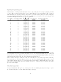
represent β values, here is the entire series assuming that 5 β values (0.8, 0.6, 0.4, 0.2, and 0.0) were visited
during the course of the analysis:
c1.0
=
c0.0
c1.0
c0.8
c0.8
c0.6
c0.6
c0.4
c0.4
c0.2
c0.2
c0.0
Note that the denominator of one ratio cancels the numerator of the adjacent ratio so that the product of
all ratios is c1.0 /c0.0 . The value c1.0 is the normalizing constant when β = 1.0, and thus is the quantity of
interest: the normalizing constant of the posterior distribution (otherwise known as the marginal likelihood).
The value c0.0 is the normalizing constant when β = 0.0 (reference distribution), which is always equal to
1.0.
Why estimate all those ratios if almost everything cancels? The answer is that, like jumping a creek, it
helps to have stepping stones. Estimating the ratio c1.0 /c0.0 is difficult because even though the reference
distribution is made to be as close as possible to the posterior, it is nevertheless very simple compared to
23
the posterior (a good deal of the correlation among parameters is missing because the reference distribution
is a product of independent probability distributions). Each ratio in the product above, however, is much
easier to estimate because the distribution on top is quite similar to the one on the bottom, a situation in
which importance sampling work well.
The steppingstone.py script
To initiate a steppingstone analysis, use the ss command instead of the mcmc command. Here is the entire
steppingstone.py script.
from phycas import *
mcmc.data_source = 'green.nex'
model.type="hky"
model.state_freqs = [0.25, 0.25, 0.25, 0.25]
model.fix_freqs = True
model.kappa = 2.0
model.kappa_prior = BetaPrime(1.0, 1.0)
model.num_rates = 4
model.gamma_shape = 0.5
model.gamma_shape_prior = Exponential(1.0)
m1 = model()
m2 = model()
model.fix_freqs = False
m3 = model()
first
= subset(1, 1296, 3)
second = subset(2, 1296, 3)
third
= subset(3, 1296, 3)
partition.addSubset(first, m1, "First codon positions")
partition.addSubset(second, m2, "Second codon positions")
partition.addSubset(third, m3, "Third codon positions")
partition()
mcmc.fix_topology = True
mcmc.starting_tree_source = TreeCollection(newick='''(1:0.31,2:0.10,(3:0.13,(4:0.09,
((5:0.10,6:0.20):0.06,(7:0.10,((8:0.05,10:0.11):0.02,9:0.08):0.06):0.04):0.04):0.05):0.03)''')
mcmc.ncycles = 1000
mcmc.sample_every = 1
mcmc.out.log = 'ss.log'
mcmc.out.log.mode = REPLACE
mcmc.out.trees = 'ss.t'
mcmc.out.trees.mode = REPLACE
mcmc.out.params = 'ss.p'
mcmc.out.params.mode = REPLACE
ss.nbetavals = 11
24
ss.xcycles = 1000
ss()
sump.out.log = 'ss.sump.log'
sump.out.log.mode = REPLACE
sump.file = 'ss.p'
sump()
Running steppingstone.py
Run the steppingstone.py in Python as described for basic.py (see section 3.2 on page 16). While it is running,
read the line-by-line explanation below.
Line-by-line explanation
Most of this script was described in the previous section (see section 3.4), so we will start with the line
containing the mcmc.fix topology setting.
mcmc.fix_topology = True
N This line tells Phycas that we wish to fix the tree topology (i.e. not allow the tree topology to change
throughout the MCMC analysis). While this is not strictly necessary, it does improve the efficiency of the
stepping stone estimation somewhat because the reference distribution can contain terms for each individual
branch length parameter, making it a much better match to the posterior. If the topology changes, then
a single distribution must be used to describe all branch length parameters. Because some branch lengths
are short, and others long, using a single distribution will necessarily have a large variance and not fit any
specific branch length marginal posterior distribution as well as a reference distribution dedicated to that
particular branch length parameter.
mcmc.starting_tree_source = TreeCollection(newick='''(1:0.31,2:0.10,(3:0.13,(4:0.09,
((5:0.10,6:0.20):0.06,(7:0.10,((8:0.05,10:0.11):0.02,9:0.08):0.06):0.04):0.04):0.05):0.03)''')
N Because we are fixing the tree topology, we should specify the tree topology that we wish to use. This
line defines a tree topology by creating a TreeCollection object containing a single tree. That single tree
is described by the string passed in via the newick argument. Tree descriptions passed in this way should
have taxa identified by numbers (starting with 1), and the numbers should reference the position of the
taxon in the data file.
Note that the tree description is broken across two lines above. Note also that the tree description is
surrounded by triple quotes (three single quote characters in a row). When Python encounters a string
defined by triple quotes, it allows line breaks inside. This is one way to handle this situation, but you could
also delete the carriage return in the middle so that the tree description occupies just one line in your file. If
the tree description string is all on one line, then you can use any kind of quotes you like: single, double, or
triple. However, if you break the string across two or more lines and you fail to use triple quotes to define
it, you will get an error message from Python (“SyntaxError: EOL while scanning string literal”).
mcmc.ncycles = 1000
N The ss command uses the mcmc command to do almost all of the work. Hence, the setting mcmc.ncycles
specifies the number of parameter update cycles devoted to each beta value visited. Note that this is the
25
number of cycles per beta value. If you specified ss.nbetavals to be 11 and mcmc.ncycles to be 1000,
then the total number of cycles would be 11 times 1000, or 11000 cycles.
This example uses 11 beta values, but is this enough? Generally the more stepping stones (i.e. beta values)
used, the better the estimate will be, but the quality of the estimate also depends on the quality of the
reference distribution. If the reference distribution approximates the posterior well, then fewer beta values
are needed (and fewer samples per beta value are needed). If the reference distribution exactly equals
the posterior, then only a single sample from the reference distribution (beta = 0.0) would be needed to
determine the marginal likelihood exactly, This utopia is never achievable because if one actually knew the
posterior distribution exactly, then one would also know the normalizing constant exactly and hence you
would not need to estimate it! In practice, it probably makes sense to start with, say, 11 β values, and a
reasonable number (e.g. 1000) cycles per β value. Then do another run, doubling both values. If this makes
a big difference, then probably the first run was not long enough (and perhaps the second run too).
mcmc.sample_every = 1
N Normally, the mcmc.sample every setting governs the degree of thinning performed. Thinning involves
ignoring some sampled parameter values in order to decrease autocorrelation or to avoid an excessive file
size. In principle, there is no reason to thin other than to keep the size of the parameter file small because
one could alway thin out the samples at a later time. Because we are not worried about the size of the
parameter file here, this line tells Phycas to save every sample (i.e. don’t thin; sample parameter values
every cycle).
mcmc.out.log = 'ss.log'
mcmc.out.log.mode = REPLACE
mcmc.out.trees = 'ss.t'
mcmc.out.trees.mode = REPLACE
mcmc.out.params = 'ss.p'
mcmc.out.params.mode = REPLACE
N The mcmc.out.log, mcmc.out.trees and mcmc.out.params settings tell Phycas to create a log file
named ss.log, a tree file named ss.t, and a parameter file named ss.p, respectively. The mcmc.out.log.mode,
mcmc.out.trees.mode, and mcmc.out.params.mode settings tell Phycas to automatically replace these files
if they already exist (the default action is to append a number to the name rather than deleting the existing
file).
ss.nbetavals = 11
N This specifies the number of “stepping stones”to use in estimating the marginal likelihood. With this
setting, the following 11 beta values would be used: 1.0, 0.9, 0.8, 0.7, 0.6, 0.5, 0.4, 0.3, 0.2, 0.1, 0.0. In (Fan
et al., 2010), the value K represents the number of intervals (or stepping stone ratios), and thus K = 10 in
this case (K = ss.nbetavals - 1).
ss.xcycles = 1000
N This represents the number of extra cycles spent on the posterior distribution. Because the reference
distribution is created based on a sample from the posterior, it may make sense to spend a little more time
on the first stepping stone (when β = 1 and the MCMC sampler is exploring the posterior) than on the
26
other β values. Our (limited) experience shows that it is not worth spending an exorbitant amount of time
on the posterior; a small sample seems to work quite well (assuming the tree topology is fixed).
ss()
N This command starts the analysis. It essentially causes the mcmc command to be run for each β value
visited.
sump.out.log = 'ss.sump.log'
sump.out.log.mode = REPLACE
N The sump.out.log setting specifies the name of the file that will hold the output of the sump command.
The sump.out.log.mode setting tells Phycas that it is Ok to go ahead and delete any ss.sump.log file that
already exists.
sump.file = 'ss.p'
sump()
N The sump command is used to summarize the parameter file produced by the ss command and calculate
the estimate of the marginal likelihood. The name of the parameter file to summarize must be supplied in
the sump.file setting. Note that we have specified ss.p here, which matches the file name specified by the
earlier mcmc.out.params setting.
Output of steppingstone.py
The file ss.sump.log contains the output of interest from this analysis. This file has three sections labeled,
respectively, Autocorrelations, Effective and actual sample sizes, and Marginal likelihood estimate. The first
and second sections are related, for it is the autocorrelations that determine the effective sample sizes. You
will note that the first line of the Effective sample sizes section (after the header line showing the β values)
provides the actual sample sizes. This is the number of times parameter values were saved while the MCMC
analysis was exploring a particular β value. The other rows in this table provide effective sample sizes. If the
MCMC samples are highly autocorrelated, then you effectively have a smaller sample size than you might
have thought given the actual sample size. To see this, imagine a perfectly autocorrelated sample in which
every sampled value is the same. In this case, you really only have a sample size of 1, even though Phycas
might have saved 2000 values. Note the last column (for β = 0). The effective sample sizes in this column
are often larger than the actual sample size. What’s up with that? If there is zero autocorrelation, then the
effective sample sizes will hover around the actual sample size. If the autocorrelation is negative, then the
effective sample size will be larger than the actual sample size. When β = 0, Phycas is sampling directly
from standard probability distributions and zero autocorrelation is expected in this case.
The last section provides some information about each of the ratios (stepping stones) that it estimated in the
process of estimating the marginal likelihood. The first column (labeled b (k-1)) is the power (i.e. value of
β) used for the distribution being sampled. You will note that β = 1 (the posterior distribution) is absent.
This is because the samples taken from the posterior are used to formulate the reference distribution, not for
estimating the individual ratios in the stepping-stone method. The column labeled beta incr shows the
difference between the current β value and the previous one. For the (default) generalized stepping-stone
method, these β increments should all be the same. The column labeled n provides the number of sample
used for that particular ratio. The column labeled lnRk is the log of the ratio of normalizing constants
corresponding to one stepping stone ratio. The product of the individual ratios equals the estimate of the
marginal likelihood. The last column, labeled lnR(cum) provides the running sum of the individual lnRk
values. The final estimate of the log of the marginal likelihood is provided at the bottom of the file.
27
3.6
Polytomy analyses
Unlike most other programs for Bayesian phylogenetic inference, Phycas can be set up to allow its Markov
chain to visit tree topologies containing polytomies. In the most extreme case, Phycas could even spend time
on the star tree (i.e. a tree with only one internal node). The reasons one might want to do this are outlined in
Lewis, Holder, and Holsinger (2005). Phycas is not the only software package out there that does this. In fact,
there are two others that I know of: Crux (written by Jason Evans, http://www.canonware.com/Crux/)
and p4 (written by Peter Foster, http://bmnh.org/˜pf/p4.html). To convert an existing phycas
Python script into one that allows polytomies, you need add only three lines:
mcmc.allow_polytomies = True
mcmc.polytomy_prior
= True
mcmc.topo_prior_C
= exp(1.0)
The setting mcmc.allow polytomies, when set to True, tells Phycas that you wish for unresolved trees to
be visited in addition to fully-resolved trees. Unresolved trees are tree topologies with at least one polytomy
(an internal node with at least four connecting edges). A fully-resolved unrooted tree has exactly three edges
connecting to each internal node. The next two lines determine the kind of topology prior you wish to use.
There are two major possibilities: (1) a polytomy prior and (2) a prior on resolution class.
The first (polytomy prior) is the easiest to understand, is the one implied by the command mcmc.polytomy prior
= True, and is the only one we will use in the following exercises. In the polytomy prior, the relative prior
probability of a tree with n internal nodes differs from the prior probability of a tree with n+1 internal nodes
by the factor mcmc.topo prior C. If mcmc.topo prior C is set equal to 1.0, then every tree topology, regardless of the number of internal nodes, would have the same prior probability. Setting mcmc.topo prior C to a
value greater than 1 favors less-resolved trees. If we used the command mcmc.topo prior C = exp(1.0),
then the factor used would be e1 (approximately 2.718), and a fully-resolved tree would need to have a
likelihood 1 unit higher (on the log scale) to be favored over a tree with one fewer internal node (and hence
1 fewer edge). To push the bar even higher, you could set mcmc.topo prior C = exp(2.0), which sets
the factor to e2 and requires a more-resolved tree to be higher by 2 log-likelihood units to equal a tree with
one more polytomy.
You might ask “Why should the prior favor less-resolved trees?” If you are tempted to perform a polytomyfriendly analysis in the first place, it is probably because you fear that a false clade will receive undue
support. In such situations, you may prefer to be conservative, not only allowing polytomous trees into the
analysis but actually making it extra hard for a false clade to receive high support.
The second possible prior allowed by Phycas is the resolution class prior. This prior not only takes
account of the number of internal nodes, but also the number of possible trees that have that particular
number of internal nodes. A tree topology in resolution class k has k internal nodes. For example, in a
4-taxon problem, there is a single star tree (resolution class 1) but 3 fully-resolved trees (resolution class 2).
Suppose you conducted an MCMC analysis for a 4-taxon problem that explored the prior, using a polytomy
prior with mcmc.topo prior C = 1. In this case, every tree topology has the same prior probability as
every other tree topology, yet the resulting sample would be dominated by fully-resolved trees! In fact, there
should be 3 times as many fully-resolved trees as unresolved (star) trees showing up in the sample there
are 3 possible unresolved trees but only 1 star tree. Using a resolution class prior, you could create a prior
that results in each resolution class being C times more probable, a priori, than the next lower resolution
class. For the 4-taxon case, making the star tree 3 times more probable than any one fully-resolved topology
results in a flat resolution class prior. An MCMC sample would contain roughly the same number of star
trees as fully-resolved trees. To use a resolution class prior, set mcmc.polytomy prior = False and set
mcmc.topo prior C to the desired ratio of adjacent resolution class priors.
28
Exploring the polytomy prior
It is instructive to run Phycas without data in order to explore the prior. Let’s begin by figuring out what
to expect. For a 5-taxon problem, there are 15 possible fully-resolved trees (resolution class 3), 10 trees
with 2 internal nodes (resolution class 2), and 1 star tree (resolution class 1). Below is a table showing the
expected results (prior probabilities of each of the 26 possible tree topologies) for both a polytomy prior and
a resolution class prior when mcmc.topo prior C equals 1.0:
Tree Number Resolution Class Tree Topology Polytomy Prior Resolution Class Prior
1
1
(1,2,3,4,5)
0.03846
0.33330
2
2
(1,2,(3,4,5))
0.03846
0.03333
3
2
(1,3,(2,4,5))
0.03846
0.03333
4
2
(1,4,(2,3,5))
0.03846
0.03333
5
2
(1,5,(2,3,4))
0.03846
0.03333
6
2
(2,3,(1,4,5))
0.03846
0.03333
7
2
(2,4,(1,3,5))
0.03846
0.03333
8
2
(2,5,(1,3,4))
0.03846
0.03333
9
2
(3,4,(1,2,5))
0.03846
0.03333
10
2
(3,5,(1,2,4))
0.03846
0.03333
11
2
(4,5,(1,2,3))
0.03846
0.03333
12
3
(1,5,(2,3,4))
0.03846
0.02222
13
3
(2,5,(1,(3,4))
0.03846
0.02222
14
3
(1,2,(5,(3,4))
0.03846
0.02222
15
3
(1,2,(3,(4,5))
0.03846
0.02222
16
3
(1,2,(4,(3,5))
0.03846
0.02222
17
3
(1,5,(3,(2,4))
0.03846
0.02222
18
3
(3,5,(1,(2,4))
0.03846
0.02222
19
3
(1,3,(5,(2,4))
0.03846
0.02222
20
3
(1,3,(2,(4,5))
0.03846
0.02222
21
3
(1,3,(4,(2,5))
0.03846
0.02222
22
3
(1,5,(4,(2,3))
0.03846
0.02222
23
3
(4,5,(1,(2,3))
0.03846
0.02222
24
3
(1,4,(5,(2,3))
0.03846
0.02222
25
3
(1,4,(2,(3,5))
0.03846
0.02222
26
3
(1,4,(3,(2,5))
0.03846
0.02222
For the polytomy prior, each of the 26 tree topologies shows up in 1/26 (3.846%) of the sample. Note that,
as a class, fully-resolved trees dominate the sample (57.7%) even though, individually, they are as frequent
as any other tree topology. That is because there are 15 tree topologies in this class (resolution class 3), but
only 10 in resolution class 2 and only 1 in resolution class 1 (the star tree).
In the resolution class prior column, note that each of the fully resolved trees shows up 2.222% of the time,
but because there are 15 of these fully-resolved tree topologies, as a class they make up 15*2.222 = 33.33%
of the sample. Likewise, the tree topologies in resolution class 2 show up individually only 3.333% of the
time, but as a class they make up 33.33%. Finally, the star tree, being alone in its resolution class, makes
up 33.33% of the sample.
The polytomy.py script
Set up an analysis that will explore one of these priors. Here is a minimal phycas Python script to explore
the resolution class prior for 5 taxa. Name this script polytomy.py.
29
from phycas import *
mcmc.allow_polytomies = True
mcmc.polytomy_prior
= False
mcmc.topo_prior_C
= 1.0
mcmc.data_source = None
mcmc.ntax = 5
mcmc.ncycles = 20000
mcmc.sample_every = 1
mcmc()
sumt.trees = 'trees.t'
sumt.burnin = 1
sumt.tree_credible_prob = 1.0
sumt()
Line-by-line explanation
from phycas import *
N This is the mandatory starting line for any Phycas Python script. It imports all the functionality defined
by Phycas into your Python implementation.
mcmc.allow_polytomies = True
N This line tells Phycas to consider unresolved trees when performing a Bayesian MCMC analysis. If this
were set to False (the default), only fully resolved trees would be allowed.
mcmc.polytomy_prior
= False
N Setting mcmc.polytomy prior to True tells Phycas that you want to use a polytomy prior. Setting
mcmc.polytomy prior to False, as we’ve done here, chooses a resolution class prior.
mcmc.topo_prior_C
= 1.0
N This sets the “strength” of the resolution class prior. Specifying 1.0 here means that each resolution
class will be represented equally in a sample from the prior. This effectively emphasizes tree topologies in
resolution classes that have fewer members. For example, even though the star tree is the only member
of the resolution class 1, it will be visited as often as the fully-resolved resolution class, which contains
a potentially huge number of tree topologies (2,027,025 unrooted, fully-resolved tree topologies for just 10
taxa). Specifying 2.0 here would mean each resolution class is twice as probable as the next higher resolution
class (by higher, I mean more resolved; i.e. having one more internal node).
mcmc.data_source = None
N Setting mcmc.data source to None (be sure to capitalize the None so that Python recognizes it) tells
Phycas that we are not specifying a data set for this analysis. The MCMC analysis will explore the prior
30
rather than the posterior in this case.
mcmc.ntax = 5
N Normally, Phycas ascertains the number of taxa from the data file, but since we are running without data
we need to tell Phycas how many taxa to assume. The mcmc.ntax setting accomplishes that.
mcmc.ncycles = 20000
N The mcmc.ncycles setting tells Phycas how many parameter update cycles to perform. Phycas will
normally update each parameter once during a single cycle, but edge length parameters make this a bit
complicated. If the tree topology is fixed, each branch length is updated once per cycle. In the present
example, the tree topology is free to vary, which means that edge lengths are updated using a MetropolisHastings proposal (the LOCAL move) that selects three edges at random to modify. This proposal is, by
default, attempted 100 times per cycle, so some edge length parameters will probably get updated more than
once, and others not at all, during a single update cycle.
mcmc.sample_every = 1
N The mcmc.sample every setting establishes how often a sample will be saved to the params.p file. In this
case, we are saving a sample after every cycles. If this setting had been 10, then we would only save a sample
after every 10 cycles.
mcmc()
N The mcmc command initiates the MCMC analysis.
sumt.trees = 'trees.t'
N The sumt command summarizes the trees and splits sampled during an MCMC analysis. This sumt.trees
setting tells the sumt command what file to summarize. The trees.t file is created by the mcmc command.
sumt.burnin = 1
N The first tree saved in a tree file produced during an MCMC analysis is the starting tree, which is never
a valid sample from the posterior distribution. Thus, the sumt.burnin setting above tells Phycas to not
count the first tree in the trees.t file. If we had specified 10 instead of 1 for the sumt.burnin setting, then
Phycas would have ignored the first ten trees it found in the trees.t file.
sumt.tree_credible_prob = 1.0
N Normally, the sumt command produces a PDF file containing a graphical representation of all trees in the
95% credible set. To determine the 95% credible set, Phycas sorts tree topologies by their marginal posterior
probability (with the largest posteriors first) and adds tree topologies to the credible set until the cumulative
posterior probability first exceeds 0.95. The sumt.tree credible prob setting tells Phycas what the cutoff
should be. The default value is 0.95, but here we are making it 1.0 so that all trees sampled will be included
in the credible set (and any summary statistics produced). Ordinarily, this might be a dangerous thing to
do. Imagine if your trees.t file contained 20000 distinct tree topologies. The resulting PDF file would be
enormous! In this case it is safe because we know there are only 15 possible tree topologies for 5 taxa.
sumt()
N This line calls the sumt. It essentially tells Phycas that we have finished setting up the sumt command
and are ready for it to run.
31
4
4.1
Reference
Probability Distributions
Phycas defines several probability distributions. Several of these (Uniform, Beta, Exponential, Gamma,
InverseGamma) are commonly used as prior distributions for model parameters. Others (Bernoulli, BetaPrime, Binomial, Normal) are less commonly used as prior distributions in Bayesian phylogenetics, but
are nevertheless useful for other reasons. This section briefly describes each of these distributions.
Terminology
The support of a distribution is the set of values for which the density function is greater than zero. A
distribution is a discrete distribution if the number of possible values is finite and each value is associated
with a non-zero probability. Discrete distributions are associated with probability functions, p(y|θ), that serve
to provide the probability associated with each possible value. A distribution is a continuous distribution
if the number of possible values is infinite and thus each particular value has probability zero. Continuous
distributions are associated with probability density functions (pdfs). The pdf, f (y|θ), provides the relative
probability of each value. The pdf is scaled so that it integrates to 1.0, allowing specific areas under the pdf
to be interpreted as probabilities. The indicator function 1x=y takes on the value 1.0 if and only if the
condition in the subscript is true (i.e., x = y in this example).
Using probability distributions in Phycas
In most cases, you will need to prefix the names of distributions with ProbDist. For example:
model.pinvar_prior = ProbDist.Beta(1,1)
You can avoid the need for the prefix by specifically importing the distributions you need at the top of your
script. For example:
from phycas.ProbDist import Beta,Gamma
...
model.pinvar_prior = Beta(1,1)
Each probability distribution defined in Phycas provides a sample method that generates a single random
deviate from that distribution. For example:
d = ProbDist.Gamma(0.5, 4.0)
d.sample()
11.923011659940444
This can be used to get a feel for typical values generated from a distribution. To generate 10 values from a
Gamma(0.5, 4.0) distribution, you can use a Python for loop:
d = ProbDist.Gamma(0.5, 4.0)
for i in range(10):
d.sample()
0.21277867604109485
1.8952730436709666
0.26548236737438019
3.2718729795327026
32
2.5822707554839197
0.043311257125495065
0.30315706776669216
14.728064587204788
0.085634607314423447
0.10030029917676343
It is also possible to get the distribution object to tell you its current mean, variance and standard deviation:
d = ProbDist.Gamma(0.5, 4.0)
d.getMean()
2.0
d.getVar()
8.0
d.getStdDev()
2.8284271247461903
To set the parameters of a distribution to match a particular mean and variance, use the setMeanAndVariance
method:
d = ProbDist.Normal(1.0, 1.0)
d.setMeanAndVariance(2.0, 1.0)
d.getMean()
2.0
d.getVar()
1.0
To get a description of the distribution and a list of all of its methods, use the help function:
help(ProbDist.Normal)
This is a class or python type
Represents the univariate normal probability distribution.
The following public methods are available:
getMean
setLot
resetLot
getDistName
getRelativeLnPDF
getVar
lnGamma
getStdDev
clone
getLnPDF
isDiscrete
sample
setMeanAndVariance
setSeed
getCDF
To get a description and usage example for a particular function, use help on the name of the function:
help(ProbDist.Exponential.setMeanAndVariance)
33
<unbound method Exponential.setMeanAndVariance>
An instance of type instancemethod.
Sets the mean and variance of this distribution. This distribution is
determined entirely by the mean, so the var argument is ignored. The
reason this function requires both mean and variance is for
compatibility with functions of the same name in other distributions.
>>> from phycas.ProbDist import *
>>> b = Exponential(2)
>>> print b.getMean()
0.5
>>> print b.getVar()
0.25
>>> b.setMeanAndVariance(5, 0)
>>> print b.getMean()
5.0
>>> print b.getVar()
25.0
4.2
Probability distributions available in Phycas
Bernoulli
This distribution is provided for completeness, but currently there are no parameters in Phycas for which this
distribution should be used as a prior. There are only two possible values (0 and 1), so Bernoulli distributions
are appropriate for modeling stochastic processes that are characterized by presence vs. absence of something,
or success vs. failure.
Type:
Discrete, univariate
Parameter:
p (probability of 1)
Probability function:
p(y|p) = p1y=1 + (1 − p)1y=0
Support:
{0, 1}
Expected value:
E[y] = p
Variance:
Var(y) = p(1 − p)
Beta
Beta distributions are popular as priors for parameters whose support is the interval [0.0, 1.0], such as
proportions. The proportion of invariable sites parameter (often abbreviated pinvar) has a Beta prior by
default in Phycas. The quantity Γ(x) that appears in the pdf is the gamma function, which for integral
values of x is equal to (x − 1)!.
34
Type:
Continuous, univariate
Parameters:
α, β
Probability density function:
f (y|α, β) =
Support:
[0.0, 1.0]
Expected value:
E[y] =
Variance:
Var(y) =
Γ(α+β)
Γ(α) Γ(β)
y α−1 (1 − y)β−1
α
α+β
αβ
(α+β)2 (α+β+1)
BetaPrime
The main use of the BetaPrime distribution in Phycas is to provide a prior distribution for the κ parameter
(the transition/transversion rate ratio in the HKY model) that is comparable to the prior used by MrBayes.
In MrBayes, the κ parameter is not given a prior directly; instead, a Beta prior is applied (by default) to
the two relative rates in the HKY rate matrix (the transition rate and the transversion rate). Specifying
a BetaPrime(a,b) prior on κ in Phycas is equivalent to specifying a Beta(a,b) prior on the transition and
transversion rates in MrBayes. You are of course free to use any other univariate distribution as a prior for
κ in Phycas; the BetaPrime distribution is only provided to make it possible to conduct Phcyas analyses
that are comparable to MrBayes analyses. Note that the mean of the BetaPrime distribution is undefined if
α is less than or equal to 1, and the variance is undefined if β is less than or equal to 2.
Type:
Continuous, univariate
Parameters:
α, β
Probability density function:
f (y|α, β) =
Support:
[0.0, 1.0]
Expected value:
E[y] =
Variance:
Var(y)
Γ(α+β) y α−1
Γ(α) Γ(β) y α+β
α
β−1
α(α+β−1)
= (β−2)(β−1)
2
Binomial
The Binomial distribution is not currently useful as a prior distribution in Phycas, and is provided for the
sake of completeness. The Binomial distribution is commonly used to model counts of the number of trials
satisfying some condition (a “success”). For example, the number of heads out of 10 (independent) flips of a
coin follows a Binomial distribution. The parameter of the distribution is the probability that the condition
(e.g. heads) is satisfied on any given trial.
Type:
Discrete, univariate
Parameters:
Probability function:
p (probability of success in any given trial), n (number of trials)
p(y|p, n) = ny py (1 − p)n−y
Support:
{0, 1, · · ·}
Expected value:
E[y] = np
Variance:
Var(y) = np(1 − p)
35
Dirichlet
The Dirichlet distribution is used as a prior for quantities that must sum to 1.0, such as state frequencies. The parameters of a Dirichlet distribution are positive real numbers. If all parameters are equal, the
Dirichlet distribution is symmetric. For example, a Dirichlet(10,10,10,10) distribution would yield samples
of nucleotide frequencies in which no one nucleotide predominates. Furthermore, if all Dirichlet parameters
equal 1, then every combination of values has equal probability density. Thus, in a Dirichlet(1,1,1,1) distribution of nucleotide frequencies, extreme frequencies (e.g. , 0.001, 0.001, 0.001, 0.997) have just as much of
a chance of showing up in a sample as equal frequencies (i.e., 0.25, 0.25, 0.25, 0.25).
Important: For multivariate distributions such as the Dirichlet distribution, you must
supply a Python list or tuple rather than a single value as the parameter. Thus, to
construct a flat Dirichlet prior for state frequencies, you either need to use an extra set of
parentheses (the inner set being recognized by Python as defining a tuple), like this:
model.state freq prior = Dirichlet((1.0, 1.0, 1.0, 1.0))
or use square brackets (recognized by Python as defining a list), like this:
model.state freq prior = Dirichlet([1.0, 1.0, 1.0, 1.0])
Type:
Continuous, multivariate
Parameters:
c1 , c2 , · · · , cn (0 < ci < ∞)
Pn
c· = i=1 ci
Probability function:
f (y1 , y2 , · · · , yn |c1 , c2 , · · · , cn ) = p1 p2 · · · pn
Support:
[0, 1]n
Expected value:
E[yi ] =
Variance:
Var(yi ) =
Covariance:
(p1 y1 )c1 −1 (p2 y2 )c2 −1 ··· (pn yn )cn −1
Γ(c1 )Γ(c2 )···Γ(cn )
Γ(c· )
ci
c·
ci (c· −ci )
c2· (c· +1)
−c cj
Cov(yi , yj ) = c2 (c·i+1)
·
Exponential
The Exponential distribution is a special case of the Gamma distribution (in which the shape parameter
equals 1.0). The Exponential distribution is a common prior for parameters whose support equals the positive
real numbers, such as edge lengths, transition/transversion rate ratio (κ), nonsynonymous/synonymous
rate ratio (ω), the shape parameter of the discretized Gamma distribution used to model among-site rate
heterogeneity, GTR model relative rates (exchangeabilities), and unnormalized parameters governing base
frequencies.
Type:
Continuous, univariate
Parameter:
λ (rate; a.k.a. hazard)
Probability function:
f (y|λ) = λe−λy
Support:
[0.0, ∞)
Expected value:
E[y] = 1/λ
Variance:
Var(y) = 1/λ2
36
Gamma
The Gamma distribution (or its special case, the Exponential distribution) is commonly used as a prior
distribution for parameters defined on the positive half of the real number line. The Gamma distribution
assigns probability zero for any value less than zero. Gamma distributions with shapes less than 1 have a
pdf mode greater than zero. Those with shape equal to 1 are identical to Exponential distributions. In this
case, the highest point reached by the pdf is β and occurs at the value zero. If the shape is greater than 1,
the pdf approaches infinity as zero is approached. The quantity Γ(α) that appears in the pdf is the gamma
function, which for integral values of α is equal to (α − 1)!.
Type:
Continuous, univariate
Parameters:
α (shape), β (scale)
Probability function:
f (y|α, β) =
Support:
[0.0, ∞)
Expected value:
E[y] = αβ
Variance:
Var(y) = αβ 2
y α−1 e−y/β
β α Γ(α)
InverseGamma
The Inverse Gamma distribution with parameters α and β is the distribution of the quantity 1/y if y has a
Gamma(α, β) distribution. In Phycas, the Inverse Gamma distribution is primarily used as an edge length
hyperprior (see section 2.2 on hierarchical models). The mean of an Inverse Gamma distribution is undefined
unless the shape parameter α is greater than 1; the variance is undefined unless α > 2.
Type:
Continuous, univariate
Parameters:
α (shape), β (scale)
Probability function:
f (y|α, β) =
Support:
[0.0, ∞)
Expected value:
E[y] =
Variance:
Var(y) =
(1/y)α+1 e−(1/y)/β
β α Γ(α)
1
β (α−1)
1
β 2 (α−1)2 (α−2)
Lognormal
Specifying a Lognormal(µ,σ) distribution for a random variable Y means that log(Y ) is normally distributed
with mean µ and variance σ 2 . It is important to remember that µ and σ do not represent the mean and
variance of the variable Y that is distributed lognormally (tricky!). Unlike the Normal distribution, which
has support (−∞,∞), the support for Lognormal is [0,∞), which makes it applicable to the same parameters
as the Gamma distribution.
37
Type:
Continuous, univariate
Parameters:
µ (mean of log(Y )), σ (standard deviation of log(Y ))
Probability function:
f (y|µ, σ) =
Support:
[0, ∞)
Expected value:
E[y] = eµ+ 2
2
2
Var(y) = eσ − 1 e2µ+σ
Variance:
√1
e−
y 2πσ 2
(log(y)−µ)2
2σ 2
σ2
Normal
The normal distribution does not get a lot of use as a prior distribution because its support includes the
negative real numbers, and most parameters used in Bayesian phylogenetics only make sense if they are
positive.
Type:
Continuous, univariate
Parameters:
µ (mean), σ (standard deviation)
Probability function:
f (y|µ, σ) =
Support:
(−∞, ∞)
Expected value:
E[y] = µ
Variance:
Var(y) = σ 2
√ 1
e−
2πσ 2
(y−µ)2
2σ 2
RelativeRate
The Relative Rate Distribution is used as a prior for the subset relative rates in a partitioned data model.
The Relative Rate Distribution is very similar to a Dirichlet distribution. A vector of relative rates has
mean equal to 1.0, however, which makes a Dirichlet distribution inappropriate (the sum, not the mean, of
the components of a Dirichlet-distributed random variable is 1). The distinction between a Relative Rate
distribution and a Dirichlet distribution mainly arises in the model selection context when the Stepping Stone
method is begin used to estimate marginal (model) likelihoods. In the Stepping Stone method, constants
that appear in prior distribution probability density functions must be fully specified. This is not necessary
for Bayesian MCMC analyses because such constants cancel out.
The quantities pi below are the subset weights. Ordinarily, pi is simply the proportion of sites assigned to
subset i. The parameter ci is analogous to the corresponding parameter in a Dirichlet distribution.
38
Important: For multivariate distributions such as the relative rate distribution, you must
supply a Python list or tuple rather than a single value as the parameter. Thus, to
construct a flat RelativeRate prior for partition subset relative rates, you either need to
use an extra set of parentheses (the inner set being recognized by Python as defining a
tuple), like this:
partition.subset relrates prior = RelativeRate((1.0, 1.0, 1.0, 1.0))
or use square brackets (recognized by Python as defining a list), like this:
partition.subset relrates prior = RelativeRate([1.0, 1.0, 1.0, 1.0])
Note that because the default is to use a RelativeRate prior for partition subset relative
rates, you need not worry about specifying anything for
partition.subset relrates prior unless you want to create a prior that is more
informative than the default (in which all parameters in the supplied tuple equal 1.0).
Type:
Continuous, multivariate
Parameters:
c1 , c2 , · · · , cn (0 < ci < ∞)
Pn
c· = i=1 ci
Probability function:
f (y1 , y2 , · · · , yn |c1 , c2 , · · · , cn ) = p1 p2 · · · pn
Support:
[0, ∞)n
Expected value:
ci
pi c·
· −ci )
Var(yi ) = pc2ic(c2 (c
· +1)
i ·
−c c
Cov(yi , yj ) = pi pj c2i(cj· +1)
·
Variance:
Covariance:
(p1 y1 )c1 −1 (p2 y2 )c2 −1 ··· (pn yn )cn −1
Γ(c1 )Γ(c2 )···Γ(cn )
Γ(c· )
E[yi ] =
Uniform
The Uniform distribution has been used extensively as a prior for many different continuous model parameters; however, because Uniform distributions must be truncated in order to be proper, their use as prior
distributions can have some surprising effects (see Felsenstein (2004) for a good discussion of the problems
with truncated Uniform priors).
Type:
Continuous, univariate
Parameters:
a (lower bound), b (upper bound)
Probability function:
f (y|a, b) =
Support:
[a, b]
Expected value:
E[y] =
Variance:
Var(y)
4.3
1
b−a
a+b
2
2
= (b−a)
12
Models
Phycas implements the standard suite of nucleotide models: JC, F81, K80, HKY, and GTR with their I, G
and I+G rate heterogeneity versions. The following sections illustrate how to set up each of the five basic
39
classes of models listed above and how to add discrete gamma and/or proportion of invariable sites rate
heterogeneity to any model.
JC
The JC model (Jukes and Cantor, 1969) constrains base frequencies and relative substitution rates to be
equal.
Rate matrix
A

A −3α
C
 α
R=
G α
T
α
C
α
−3α
α
α
G
α
α
−3α
α
T

α
α 

α 
−3α
Choosing the JC model in Phycas
model.type = 'jc'
F81
The F81 model (Felsenstein, 1981) constrains relative substitution rates (µ) to be equal but allows base
frequencies (π) to vary. Fixing πA = πC = πG = πT = 0.25 makes the F81 model equivalent to the JC
model (note that µ = 4α).
Rate matrix
A

C
G
T
P

A − i6=A πi µ
πG µ
πT µ
PπC µ

C
πA µ
− i6=C πi µ
πT µ


PπG µ
R=

G
πA µ
πC µ
− i6=G πi µ
π
µ
T
P
T
πA µ
πC µ
πG µ
− i6=T πi µ
Choosing the F81 model in Phycas
model.type = 'hky'
model.kappa = 1.0
model.fix_kappa = True
K80
The K80 model (Kimura, 1981) constrains base frequencies to be equal but allows the rate of transitions to
differ from the rate of transversions by a factor κ = α/β.
Rate matrix
A
A −β(κ + 2)
C
β

R=
G
βκ
T
β

C
β
−β(κ + 2)
β
βκ
40
G
βκ
β
−β(κ + 2)
β
T

β

βκ


β
−β(κ + 2)
Choosing the K80 model in Phycas
model.type = 'hky'
model.state_freqs = [0.25, 0.25, 0.25, 0.25]
model.fix_freqs = True
HKY
The HKY model (Hasegawa et al., 1985) allows base frequencies to be unequal and the transition/transversion
rate ratio κ to be some value other than 1.0.
Rate matrix
A
C
G
T

A −β(πY + πG κ)
πC β
πG β κ
πT β

C
πA β
−β(πR + πT κ)
πG β
πT β κ


R=


G
πA β κ
πC β
−β(πY + πA κ)
πT β
T
πA β
πC β κ
πG β
−β(πR + πC κ)

Choosing the HKY model in Phycas
model.type = 'hky'
GTR
The GTR model (Lanave et al., 1984) allows base frequencies to be unequal and all six relative substitution
rates (a, b, c, d, e and f ) to be different.
Rate matrix
A
C
G
T


A −(πC a + πG b + πT c)
πC a
πG b
πT c

C
πA a
−(πA a + πG d + πT e)
πG d
πT e


R=

G
πA b
πC d
−(πA b + πC d + πT f )
πT f
T
πA c
πC e
πG f
−(πA c + πC e + πG f )
Choosing the GTR model in Phycas
model.type = 'gtr'
Proportion of invariable-sites
A “+I” version (Reeves, 1992) of any of the basic substitution models means that each site is viewed as
having probability pinvar of being invariable (i.e. substitution rate zero). This is one common way to
accommodate among-site rate heterogeneity in nucleotide sequence data.
model.pinvar_model = True
41
Discrete gamma
A “+G” version (Yang, 1994) of any of the basic substitution models means that the model assumes that
the distribution of rates across sites conforms to a Gamma distribution having mean 1.0. In Phycas (as in
most phylogenetic software), a discretized Gamma distribution is used in practice, and implemented as an
equal weight mixture model (each site is assumed to belong to each rate category with probability 1/ncat ).
The number of rate categories ncat is set using the model.num rates option. If model.num rates is set to
any value greater than 1, the model becomes a +G version.
model.num_rates = 4
4.4
Settings
This section lists all currently available Phycas settings. You will find more if you look at the Phycas. init
method in the Phycas.py file, but be forewarned that settings found in Phycas.py but not listed here are
experimental and not fully tested — use at your own risk. Please do not ask for help with undocumented
settings: we will document them here when we feel they are ready to be used.
4.5
Settings used by like
Input options:
rng A pseudo-random number generator instance (default: None)
random seed Determines the random number seed used; specify 0 to generate seed automatically from
system clock (default: 0)
data source The DataSource that provides the data, to be used in the MCMC analysis. Should be a
DataSource object (default: None)
model Specifies the model to use. By default, uses the predefined model object. Type model.help to set the
settings for this model. (default: predefined model object)
tree source TreeCollection that will provide the tree. (default: collection of tree(s) simulated by
from the Yule process with edge lengths drawn from Exponential(10.00000))
starting edgelen dist Used to select the starting edge lengths when tree source is ’random’ (default:
Exponential(10.00000))
store site likes If True, site log-likelihoods will be stored and can be retrieved using the getSiteLikes()
function (default: False)
uf num edges Number of edges to traverse before taking action to prevent underflow (default: 50)
4.6
Settings used by mcmc
Input options:
rng A pseudo-random number generator instance (default: None)
random seed Determines the random number seed used; specify 0 to generate seed automatically from
system clock (default: 0)
42
burnin The number of update cycles to ignore before sampling begins. If burnin=1000 and ncycles=10000,
the total number of cycles will be 11000. (default: 0)
ncycles The number of update cycles (a cycle is analogous to, but different than, a ’generation’ in MrBayes;
Phycas does in one cycle what MrBayes does in about 100 generations for a simple model such as JC)
(default: 10000)
sample every The current tree topology and model parameter values will be sampled after this many cycles
have elapsed since the last sample was taken (default: 100)
report every A progress report will be displayed after this many cycles have elapsed since the last progress
report (default: 100)
verbose You will get more output if True, less output if False (default: True)
quiet If True, output will only be sent to the log file if open (see below); if False, output will be sent to the
console as well (default: False)
model Specifies the model to use. By default, uses the predefined model object. Type model.help to set the
settings for this model. (default: predefined model object)
partition Specifies the partition to use. By default, uses the predefined partition object.
<phycas.Phycas.Partition.Partition object at 0x1dafcf0>)
(default:
data source The DataSource that provides the data, if any, to be used in the MCMC analysis. Should be
a DataSource object (default: None)
starting tree source A TreeCollection that will serve as the source of the starting tree topology. If a
string is passed in, it is interpreted as a the path to a file with trees. (default: None)
tree topology Unused unless starting tree source is ’usertree’, in which case this should be a standard
newick string representation of the tree topology; e.g. ’(A:0.01,B:0.071,(C:0.013,D:0.021):0.037)’ (default: None)
fix topology If True, an EdgeMove move will be substituted for the LargetSimonMove, so edge lengths
will be updated by slice sampling but the topology will remain unchanged during an MCMC analysis
(default: False)
ls move lambda Sets the minimum value of the tuning parameter for the LargetSimonMove MetropolisHastings move. This value corresponds to a boldness vlaue of 0.0 and is the value used for normal
analyses. (default: 0.2)
ls move lambda0 Sets the maximum value of the tuning parameter for the LargetSimonMove MetropolisHastings move. This value corresponds to a boldness value of 100.0 and is only used during path
sampling analyses. (default: 1.0)
ls move weight Larget-Simon moves will be performed this many times per cycle (default: 100)
ls move debug If set to true, TreeViewer will popup on each Larget-Simon move update showing edges
affected by the proposed move (default: False)
edge move lambda Sets the minimum value of the tuning parameter for the EdgeMove Metropolis-Hastings
move. This value corresponds to a boldness vlaue of 0.0 and is the value used for normal analyses.
(default: 0.2)
43
edge move lambda0 Sets the maximum value of the tuning parameter for the EdgeMove Metropolis-Hastings
move. This value corresponds to a boldness value of 0.0 and is only used during path sampling analyses.
(default: 1.0)
edge move weight Only used if fix topology is True. Makes sense to set this to some multiple of the number
of edges since each EdgeMove affects a single randomly-chosen edge (default: 0)
nchains The number of Markov chains to run simultaneously. One chain serves as the cold chain from
which samples are drawn, the other chains are heated to varying degrees and serve to enhance mixing
in the cold chain. (default: 1)
rel rate weight Updates of GTR relative rates will occur this many times per cycle if relative rates are
being updated jointly (default: 1)
rel rate psi Sets the maximum value of the tuning parameter for the RelRatesMove Metropolis-Hastings
move. This value corresponds to a boldness value of 0.0 and is the value used for normal analyses.
(default: 300.0)
rel rate psi0 Sets the minimum value of the tuning parameter for the RelRatesMove Metropolis-Hastings
move. This value corresponds to a boldness vlaue of 100.0 and is only used during path sampling
analyses. (default: 1.0)
subset relrates weight Updates of th vector of partition subset relative rates will occur this many times
per cycle (default: 1)
subset relrates psi Sets the maximum value of the tuning parameter for the SubsetRelRatesMove MetropolisHastings move. This value corresponds to a boldness value of 0.0 and is the value used for normal
analyses. (default: 300.0)
subset relrates psi0 Sets the minimum value of the tuning parameter for the SubsetRelRatesMove MetropolisHastings move. This value corresponds to a boldness vlaue of 100.0 and is only used during path
sampling analyses. (default: 1.0)
state freq weight Updates of state frequencies will occur this many times per cycle if state frequencies
are being updated jointly (default: 1)
state freq psi Sets the maximum value of the tuning parameter for the RelRatesMove Metropolis-Hastings
move. This value corresponds to a boldness value of 0.0 and is the value used for normal analyses.
(default: 300.0)
state freq psi0 Sets the minimum value of the tuning parameter for the RelRatesMove Metropolis-Hastings
move. This value corresponds to a boldness vlaue of 100.0 and is only used during path sampling analyses. (default: 1.0)
tree scaler lambda Sets the minimum value of the tuning parameter for the TreeScalerMove MetropolisHastings move. This value corresponds to a boldness vlaue of 0.0 and is the value used for normal
analyses. (default: 0.5)
tree scaler lambda0 Sets the maximum value of the tuning parameter for the TreeScalerMove MetropolisHastings move. This value corresponds to a boldness value of 100.0 and is only used during path
sampling analyses. (default: 1.0)
tree scaler weight Whole-tree scaling will be performed this many times per cycle (default: 0)
44
allow polytomies If True, do Bush moves in addition to Larget-Simon moves; if False, do Larget-Simon
moves only (default: False)
polytomy prior If True, use polytomy prior; if False, use resolution class prior (default: True)
topo prior C Specifies the strength of the prior (C = 1 is flat prior; C > 1 favors less resolved topologies)
(default: 2.0)
bush move edgelen mean Specifies mean of exponential edge length generation distribution used by BushMove when new edges are created (default: 1.0)
bush move weight Bush moves will be performed this many times per cycle if (default: 100)
bush move debug If set to true, TreeViewer will pop up on each Bush move update showing edges affected
by the proposed move (default: False)
slice weight Slice sampled parameters will be updated this many times per cycle (default: 1)
slice max units Max. number of units used in slice sampling (default: 1000)
adapt first Adaptation of slice samplers is performed the first time at cycle adapt first. Subsequent
adaptations wait twice the number of cycles as the previous adaptation. Thus, adaptation n occurs at
cycle adapt first*(2**(n - 1)). The total number of adaptations that will occur during an MCMC run
is [ln(adapt first + ncycles) - ln(adapt first)]/ln(2) (default: 100)
adapt simple param Slice sampler adaptation parameter (default: 0.5)
min heat power Power of the hottest chain when nchains > 1 (default: 0.5)
heat vector List of heating powers, one of which should be 1.0 (default value None causes this vector to
be generated using min heat pwer) (default: None)
uf num edges Number of edges to traverse before taking action to prevent underflow (default: 50)
ntax To explore the prior, set to some positive value. Also set data source to None (default: 0)
ndecimals Number of decimal places used for sampled parameter values (default: 8)
save sitelikes Saves file of site log-likelihoods (name determined by mcmc.out.sitelikes) that sump command can use in computing conditional predictive ordinates (default: False)
Output options:
out.level Controls the amount of output (verbosity) of the command (default: OutFilter.NORMAL)
out.log The file specified by this setting saves the console output generated by mcmc(). If set to None,
console output will not be saved to a file.
out.log.prefix file prefix (appropriate suffix will be added) (default :None)
out.log.filename The full file name. Specifying this field preempts ‘prefix‘ setting.
out.log.mode Controls the behavior when the file is present. Valid settings are REPLACE, APPEND, or
ADD NUMBER. ADD NUMBER indicates that a number will be added to the end of the file name
(or prefix) to make the name uniqueADD NUMBER
45
out.trees The nexus tree file in which all sampled tree topologies are saved. This file is equivalent to the
MrBayes *.t file.
out.trees.prefix file prefix (appropriate suffix will be added) (default :None)
out.trees.filename The full file name. Specifying this field preempts ‘prefix‘ setting.
out.trees.mode Controls the behavior when the file is present. Valid settings are REPLACE, APPEND,
or ADD NUMBER. ADD NUMBER indicates that a number will be added to the end of the file name
(or prefix) to make the name uniqueADD NUMBER
out.params The text file in which all sampled parameter values are saved. This file is equivalent to the
MrBayes *.p file.
out.params.prefix file prefix (appropriate suffix will be added) (default :None)
out.params.filename The full file name. Specifying this field preempts ‘prefix‘ setting.
out.params.mode Controls the behavior when the file is present. Valid settings are REPLACE, APPEND,
or ADD NUMBER. ADD NUMBER indicates that a number will be added to the end of the file name
(or prefix) to make the name uniqueADD NUMBER
out.sitelikes The text file in which all sampled site log-likelihood values are saved.
out.sitelikes.prefix file prefix (appropriate suffix will be added) (default :None)
out.sitelikes.filename The full file name. Specifying this field preempts ‘prefix‘ setting.
out.sitelikes.mode Controls the behavior when the file is present. Valid settings are REPLACE, APPEND, or ADD NUMBER. ADD NUMBER indicates that a number will be added to the end of the
file name (or prefix) to make the name uniqueADD NUMBER
4.7
Settings used by model
Input options:
type Can be ’jc’, ’hky’, ’gtr’ or ’codon’ (default: ’hky’)
update relrates separately If True, GTR relative rates will be individually updated using slice sampling;
if False, they will be updated jointly using a Metropolis-Hastings move (generally both faster and
better). (default: True)
relrate prior The joint prior distribution for all six GTR relative rate parameters. Used only if update relrates separately is False. (default: Dirichlet((1.00000, 1.00000, 1.00000, 1.00000, 1.00000,
1.00000)))
relrate param prior The prior distribution for individual GTR relative rate parameters. Used only if
update relrates separately is true. (default: Exponential(1.00000))
relrates The current values for GTR relative rates. These should be specified in this order: A<->C,
A<->G, A<->T, C<->G, C<->T, G<->T. (default: [1.0, 4.0, 1.0, 1.0, 4.0, 1.0])
fix relrates If True, GTR relative rates will not be modified during the course of an MCMC analysis
(default: False)
46
kappa prior The prior distribution for the kappa parameter in an HKY model (default: Exponential(1.00000))
kappa The current value for the kappa parameter in an HKY model (default: 4.0)
fix kappa If True, the HKY kappa parameter will not be modified during the course of an MCMC analysis
(default: False)
omega prior The prior distribution for the omega parameter in a codon model (default: Exponential(20.00000))
omega The current value for the omega parameter in a codon model (default: 0.05)
fix omega If True, the omega parameter will not be modified during the course of an MCMC analysis
(default: False)
num rates The number of relative rates used for the discrete gamma rate heterogeneity submodel; default
is rate homogeneity (i.e. 1 rate) (default: 1)
gamma shape prior The prior distribution for the shape parameter of the gamma among-site rate distribution (default: Exponential(1.00000))
gamma shape The current value for the gamma shape parameter (default: 0.5)
fix shape If True, the gamma shape parameter will not be modified during the course of an MCMC analysis
(default: False)
use inverse shape If True, gamma shape prior is applied to 1/shape rather than shape (default: False)
pinvar model If True, an invariable sites submodel will be applied and the parameter representing the
proportion of invariable sites will be estimated (default: False)
pinvar prior The prior distribution for pinvar, the proportion of invariable sites parameter (default: Beta(1.00000,
1.00000))
pinvar The current value of pinvar, the proportion of invariable sites parameter (default: 0.2)
fix pinvar If True, the proportion of invariable sites parameter (pinvar) will not be modified during the
course of an MCMC analysis (default: False)
update freqs separately If True, state frequencies will be individually updated using slice sampling; if
False, they will be updated jointly using a Metropolis-Hastings move (generally both faster and better).
(default: True)
state freq prior The joint prior distribution for the relative state frequency parameters. Used only if
update freqs separately is False. (default: Dirichlet((1.00000, 1.00000, 1.00000, 1.00000)))
state freq param prior The prior distribution for the individual base frequency parameters; these parameters, when normalized to sum to 1, represent the equilibrium proportions of the nucleotide states.
Used only if update freqs separately is True. (default: Exponential(1.00000))
state freqs The current values for the four base frequency parameters (default: [1.0, 1.0, 1.0, 1.0])
fix freqs If True, the base frequencies will not be modified during the course of an MCMC analysis (default:
False)
47
edgelen hyperprior The prior distribution for the hyperparameter that serves as the mean of an Exponential edge length prior. If set to None, a non-hierarchical model will be used with respect to edge
lengths. Note that specifying an edge length hyperprior will cause internal and external edge length
priors to be Exponential distributions (regardless of what you assign to internal edgelen prior, external edgelen prior or edgelen prior). (default: InverseGamma(2.10000, 0.90909))
separate edgelen hyper If True, hyperparameters will be allowed to differ for internal vs. external edge
lengths. If False, one hyperparameter will govern all edge length prior distributions. If edgelen hyperprior
is None, this setting will have no effect. (default: False)
fix edgelen hyperparam If True, the hyperparameter that governs the mean of the Exponential edge length
prior will be fixed at the value edgelen hyperparam. (default: False)
edgelen hyperparam The current value of the edge length hyperparameter - setting this currently has no
effect (default: 0.05)
internal edgelen prior Can be used to set a prior distribution for internal edges that differs from that applied to external edges. If this is set to something besides None, you should also set external edgelen prior
appropriately. Setting the edgelen prior option sets both external edgelen prior and internal edgelen prior
to the same value (default: Exponential(2.00000))
external edgelen prior Can be used to set a prior distribution for external edges that differs from
that applied to internal edges. If this is set to something besides None, you should also set internal edgelen prior appropriately. Setting the edgelen prior option sets both external edgelen prior and
internal edgelen prior to the same value (default: Exponential(2.00000))
edgelen prior Sets both internal edgelen prior and external edgelen prior to the supplied value. Use this
setting if you want all edges in the tree to have the same prior distribution. Using this setting will
overwrite any values previously supplied for internal edgelen prior and external edgelen prior (default:
None)
fix edgelens not yet documented (default: False)
4.8
Settings used by randomtree
Input options:
rng A pseudo-random number generator instance (default: None)
random seed Determines the random number seed used; specify 0 to generate seed automatically from
system clock (default: 0)
distribution ’Yule’ or ’Equiprobable’ – The name of the tree generation process or distribution from which
the trees will be drawn (default: ’Yule’)
taxon labels The names of the taxa to simulate (default: [])
edgelen dist Used to generate edge lengths. This can be None if distribution = ’yule’; in this case the
branch lengths from the Yule process will be used (default: Exponential(10.00000))
speciation rate The rate of speciation that governs the branch lengths of the Yule tree simulation process.
This is only used if edgelen dist is None (default: None)
48
n trees The number of trees to generate (if 0 is specified, a bottomless collection of trees is generated)
(default: 0)
n taxa The number of taxa to generate (only used if the taxon labels attribute is not specified) (default: 0)
newick Tree topology to simulate branch lengths on. (default: None)
Output options:
out.level Controls the amount of output (verbosity) of the command (default: OutFilter.NORMAL)
4.9
Settings used by ss
Input options:
nbetavals The number of values beta will take on during the run; for example, if this value is 4, then beta
will take on these values: 1, 2/3, 1/3, 0 (default: 101)
ti If True, the marginal likelihood will be estimated using thermodynamic integration and the stepping
stone method with reference distribution equal to the prior; if False (the default), the stepping stone
method with reference distribution approximating the posterior will be used (this greatly improves the
accuracy of the stepping stone method and is strongly recommended). (default: False)
xcycles The number of extra cycles (above and beyond mcmc.ncycles) that will be spent exploring the
posterior (additional posterior cycles help stepping stone analyses formulate an effective reference
distribution). (default: 0)
maxbeta The first beta value that will be sampled. (default: 1.0)
minbeta The last beta value that will be sampled. (default: 0.0)
minsample Minimum sample size needed to create a split-specific edge length working prior. (default: 10)
shape1 The first shape parameter of the distribution used to determine the beta values to be sampled. This
distribution is, confusingly, a Beta distribution. Thus, if both shape1 and shape2 are set to 1, beta
values will be chosen at uniform intervals from minbeta to maxbeta. (default: 1.0)
shape2 The second shape parameter of the distribution used to determine the beta values to be sampled.
This distribution is, confusingly, a Beta distribution. Thus, if both shape1 and shape2 are set to 1,
beta values will be chosen at uniform intervals from minbeta to maxbeta. (default: 1.0)
4.10
Settings used by sump
Input options:
burnin Number of lines from the input list of trees to skip (first line stores starting parameter values, so
this value should normally be at least 1) (default: 1)
file Name of file containing sampled parameter values (default: ’’)
cpofile Name of file containing sampled site likelihoods for calculation of Conditional Predictive Ordinates
(CPO) (default: ’’)
49
Output options:
out.level Controls the amount of output (verbosity) of the command (default: OutFilter.NORMAL)
out.log The file specified by this setting saves the console output generated by sump(). If set to None,
console output will not be saved to a file.
out.log.prefix file prefix (appropriate suffix will be added) (default :None)
out.log.filename The full file name. Specifying this field preempts ‘prefix‘ setting.
out.log.mode Controls the behavior when the file is present. Valid settings are REPLACE, APPEND, or
ADD NUMBER. ADD NUMBER indicates that a number will be added to the end of the file name
(or prefix) to make the name uniqueADD NUMBER
out.cpoplot The file specified by this setting saves the R commands to produce a plot of CPO values across
sites. If set to None, no R file will be generated.
out.cpoplot.prefix file prefix (appropriate suffix will be added) (default :None)
out.cpoplot.filename The full file name. Specifying this field preempts ‘prefix‘ setting.
out.cpoplot.mode Controls the behavior when the file is present. Valid settings are REPLACE, APPEND,
or ADD NUMBER. ADD NUMBER indicates that a number will be added to the end of the file name
(or prefix) to make the name uniqueADD NUMBER
4.11
Settings used by sumt
Input options:
outgroup taxon Set to the taxon name of the tip serving as the outgroup for display rooting purposes (note:
at this time outgroup can consist of just one taxon) (default: None)
trees A source of trees (list of trees or to the name of the input tree file) to be summarized. This setting
should not be None at the time the sumt method is called. (default: None)
burnin Number of trees from the input list of trees to skip (default: 1)
tree credible prob Include just enough trees in the <sumt trees prefix>.tre and <sumt trees prefix>.pdf
files such that the cumulative posterior probability is greater than this value (default: 0.95)
useGUI If True, and if wxPython is installed, a graphical user interface (GUI) will be used to display, and
allow manipulation of, AWTY plots (default: True)
rooted Set to True if trees are rooted; otherwise, leave set to default value of False to assume trees are
unrooted (default: False)
Output options:
out.level Controls the amount of output (verbosity) of the command (default: OutFilter.NORMAL)
out.log The file specified by this setting saves the console output generated by sumt(). If set to None,
console output will not be saved to a file.
50
out.log.prefix file prefix (appropriate suffix will be added) (default :None)
out.log.filename The full file name. Specifying this field preempts ‘prefix‘ setting.
out.log.mode Controls the behavior when the file is present. Valid settings are REPLACE, APPEND, or
ADD NUMBER. ADD NUMBER indicates that a number will be added to the end of the file name
(or prefix) to make the name uniqueADD NUMBER
out.trees The output tree file in which all distinct tree topologies are saved along with the majorityrule consensus tree will be named <sumt trees prefix>.tre and the corresponding pdf file containing
graphical representations of these trees will be named <sumt trees prefix>.pdf. This setting cannot
be None when the sumt method is called.
out.trees.prefix file prefix (appropriate suffix will be added) (default :None)
out.trees.filename The full file name. Specifying this field preempts ‘prefix‘ setting.
out.trees.mode Controls the behavior when the file is present. Valid settings are REPLACE, APPEND,
or ADD NUMBER. ADD NUMBER indicates that a number will be added to the end of the file name
(or prefix) to make the name uniqueADD NUMBER
out.trees.equal brlens If True, trees in pdf file will be drawn with branch lengths equal, making support
values easier to see; if set to True, consider setting pdf scalebar position = None (scalebar is irrelevant
in this case) (default: False)
out.splits The pdf file showing plots depicting split posteriors through time and split sojourns will be
named <sumt splits prefix>.pdf. If None, this analysis will be skipped.
out.splits.prefix file prefix (appropriate suffix will be added) (default :None)
out.splits.filename The full file name. Specifying this field preempts ‘prefix‘ setting.
out.splits.mode Controls the behavior when the file is present. Valid settings are REPLACE, or ADD NUMBER.
ADD NUMBER indicates that a number will be added to the end of the file name (or prefix) to make
the name uniqueADD NUMBER
5
Design principles
The design principles underlying Phycas are presented best as a series of questions and answers.
5.1
Why was Phycas written as an extension to Python?
Most phylogenetic analyses take a considerable amount of time to run, and thus most phylogenetic analysis
software provides a mechanism for batch processing. Batch processing is ordinarily accomplished through
the use of a command syntax of some sort that allows the user to specify the sequence of commands to
run. For example, PAUP* allows PAUP blocks to be placed in NEXUS files. The user can run an analysis
without manual intervention by simply executing such a file containing PAUP* commands. This mode has
the added benefit of creating a record of exactly the analysis performed, so that later on when the reviews
come back and you are trying to respond to reviewers’ concerns, you can actually recall what you did! Using
menu-driven programs makes this difficult unless the software saves a history of all keystrokes and menu
selections. Other popular programs have their own, private command languages. For example, MrBayes
uses MRBAYES blocks in NEXUS files, Hy-Phy uses a C-like language, and Beast uses xml as its medium
51
for communicating commands. One reason we chose to extent Python is so that we could use an existing,
well-documented, widely-available computing language as the command language for Phycas. There are
many books available on using Python, which means we do not have to provide all the details, and Python is
a very powerful computing language, meaning you can write very sophisticated scripts that do anything your
heart desires in your phylogenetic analysis. With the phylogenetic library of tools supplied by Phycas, you
can even invent new phylogenetic methods if you are so inclined. There is, of course, some program-specific
learning you must do in order to use Phycas; just having a prior knowledge of Python will not save you from
reading this manual to learn what Phycas offers and how to access those features. We feel, however, that
using a powerful, existing computing language to communicate with Phycas instead of “rolling our own”
program-specific language was a very good idea.
5.2
Why is there no graphical user interface (GUI)?
Due to the large scale at which DNA sequencing is performed these days, and the increasing desire to
“pipeline” analyses, we felt that using a script-based approach would best serve the needs of potential users
in the near and distant future. Python is already installed on most unix-based operating systems (including
Linux and MacIntosh OSX), and thus Phycas can be easily inserted into bioinformatics pipeline applications.
Although it does not come pre-installed on new systems, Python is easy to install on WindowsTM -based PCs,
and thus Phycas can be used easily on any workstation or laptop. While many users like user-friendly GUIs
with pull-down menus and dialog boxes, software that depends on a GUI has certain disadvantages: (1)
cannot be pipelined easily; (2) cannot be run on a remote cluster; and (3) often does not allow one to save a
record of the exact analysis performed. One of the strong benefits of a GUI is that it allows experimentation
and visualization. Phycas provides for visualization by outputting trees and plots in the form of PDF files.
While not quite as appealing as an on-screen visual representation, PDF files provide what most of us really
need: the ability to insert a publication-quality figure into a manuscript, or load artwork into other programs
for manipulation.
5.3
Is Phycas slower than MrBayes?
All scripting-based languages (R, Python, Perl, Ruby) are relatively slow compared to compiled languages
such as C and C++. Fortunately, the Boost Python library (http://www.boost.org/libs/python/
doc/) has made it easy to write the parts of Phycas that need to be fast in C++ and export these routines so
that they can be called from Python. As a result, Phycas competes favorably with any phylogenetic software
application out there in terms of speed. If you make speed comparisons of Phycas to other programs, be sure
to compare them in a fair way. Phycas uses a different definition of “generation” than does MrBayes, for
example. Because a “cycle” in Phycas is equivalent to more than 100 “generations” in MrBayes, it is easy to
conclude that Phycas is slow compared to MrBayes. To be fair, compare instead the time required for some
(large) number likelihood calculations under comparable models. Phycas makes this easy by reporting the
number of likelihood calculations performed and the time required at the end of an MCMC analysis. The
number of likelihood calculations used by MrBayes for a single chain equals simply the number of generations.
6
6.1
Installing Phycas
Instructions for WindowsTM users
These instructions assume you are using WindowsTM XPTM or VistaTM .
52
WindowsTM console
One very handy feature that does not come with WindowsTM is the ability to open a command console
by using the right-click speed menu in ExplorerTM . The web site http://www.commandline.co.uk/
cmdhere/ describes how to add this functionality, which will make Phycas much easier to use (it is not
required, however, in order to use Phycas). The basic procedure is to create a file named cmdhere.reg with
the following text (or download the file from the web site above):
REGEDIT4
[HKEY_CLASSES_ROOT\*\shell\cmdhere]
@="Cmd&Here"
[HKEY_CLASSES_ROOT\*\shell\cmdhere\command]
@="cmd.exe /c start cmd.exe /k pushd \"%L\\..\""
[HKEY_CLASSES_ROOT\Folder\shell\cmdhere]
@="Cmd&Here"
[HKEY_CLASSES_ROOT\Folder\shell\cmdhere\command]
@="cmd.exe /c start cmd.exe /k pushd \"%L\""
Assuming that you saved this file with the extension .reg, the WindowsTM operating system will know what
to do with it. Double-click the name of the file in WindowsTM ExplorerTM , and the required registry entry
will be made. Warning: making changes to your system’s registry is a bit risky, and we take
no responsibility for any damage your system may incur by following these directions! That
said, this worked fine for us and saves an enormous amount of time. WindowsTM offers a PowerToy (http:
//www.microsoft.com/windowsxp/downloads/powertoys/xppowertoys.mspx) for XPTM that
does something similar. While perhaps safer to install, it is somewhat frustrating to use because if you are
already inside a directory in which you want to open a console, you must first go up one level in order to
open a console window for that directory.
Installing Python under WindowsTM
Before you go to the trouble of downloading and installing Python, make sure you do not already have Python
installed on your Windows system. From the Start button, choose All Programs, then Accessories and finally
Command Prompt. Type python -V in the console window that appears, and if a phrase such as Python
2.5.1 appears, then you already have Python installed! Most Windows users will probably see ’python’
is not recognized as an internal or external command, operable program or batch
file. In this case, you need to visit http://python.org and download and install the latest version of
Python (version 2.6.1 as of this writing). Warning: Do not install Python 3.x — Phycas is not yet
ready to make the leap to Python 3
Installing Phycas under WindowsTM
Visit the Download section of the Phycas web site http://phycas.org/ and download the Windows
installer. If you are using Windows XP, double-click the installer to install Phycas. If using Vista, right-click
the installer and choose to install as Administrator. The installer will attempt to identify the location of
Python on your system, and if it fails to find Python will abort the installation. Assuming it can find Python,
it will install Phycas into the Lib/site-packages directory of that Python installation.
53
Locating the “Phycas Installation Folder” under WindowsTM
You will find a Phycas section in the menu that appears when you choose Start and All Programs. Included
in the Start/All Programs/Phycas menu is an item named Phycas Installation Folder. Choosing this menu item
will open WindowsTM (file) Explorer to the “Phycas Installation Folder” mentioned in the tutorial.
6.2
Instructions for MacIntosh Users
These instructions assume you are using MacOS 10.4 or later.
The iTerm terminal application
Bundled with Phycas is a terminal application called iTerm. The iTerm application is an open-source
replacement for the Terminal application with which you may be familiar (and which comes with the MacOS).
While it is possible to use Phycas from Terminal, we recommend strongly that you use the iTerm application
that comes with Phycas. The iTerm application starts automatically when you click on the icon labeled
“Phycas” (see below) or drop a script file onto the icon. The main reason for using the bundled iTerm
application is that it starts Python and imports phycas for you automatically when it is started.
Installing Python on a Mac
If you are using MacOS 10.4, and haven’t installed Python yourself, your Mac probably has Python 2.3
installed. To find out, open a terminal window (you can find the Terminal app in the Utilities folder, which
is itself a subfolder of the Applications folder) and type python -V. If the version of Python is 2.3, you will
need to visit http://python.org and download and install the latest version of Python (version 2.6.1 as
of this writing). Warning: Do not install Python 3.x — Phycas is not yet ready to make the
leap to Python 3
Installing Phycas on a Mac
Visit the Download section of the Phycas web site http://phycas.org/ and download the MacOS DMG
file. Once the DMG file has been downloaded, double-click it to mount it. Inside the DMG, you should
find several files (Figure 1). Copy the “file” named Phycas (which is actually a special “application bundle”
folder named Phycas.app, but the operating system hides the .app part of the name) to your Applications
folder and the file named manual.pdf to a folder of your choice. To start Phycas, double-click the Phycas.app
application or, alternatively, drop a script file with Phycas commands onto it. Important: When you
start Phycas, you are actually starting an application named iTerm that has been bundled with
the Phycas Python libraries. Thus, the menu items you see are iTerm menu items (including
the Update... menu item). With this MacOS version, you need not type the from phycas import *
command because this is done for you when you double-click Phycas.app.
Locating the “Phycas Installation Folder” on a Mac
The “Phycas Installation Folder” that is mentioned in the tutorial is inside the Phycas.app application bundle.
MacOS tries to make it difficult for you to see inside application bundles, but clicking on the Phycas.app
bundle while pressing the Ctrl will produce a menu, and choosing the Show Package Contents item on that
54
Figure 1: The Phycas DMG file after it has been mounted.
menu will allow you to view the contents of the application bundle folder. Once inside Phycas.app, doubleclick on the Contents folder, then the Resources folder to find the Phycas Installation folder, which is simply
named phycas.
55
References
Fan, Y., R. Wu, M.-H. Chen, L. Kuo, and P. O. Lewis. 2010. Choosing among partition models in Bayesian
phylogenetics. Molecular Biology and Evolution (in press).
Felsenstein, J. 1981. Evolutionary trees from DNA sequences: a maximum likelihood approach. Journal of
Molecular Evolution 17:368–376.
Felsenstein, J. 2004. Inferring phylogenies. Sinauer Associates, Sunderland, Massachusetts.
Hasegawa, M., H. Kishino, and T. Yano. 1985. Dating of the human-ape splitting by a molecular clock of
mitochondrial DNA. Journal of Molecular Evolution 22:160–174.
Holder, M. T., J. Sukumaran, and P. O. Lewis. 2008. A Justification for Reporting the Majority-Rule
Consensus Tree in Bayesian Phylogenetics. Systematic Biology 57:814–821.
Jukes, T. H. and C. R. Cantor. 1969. Evolution of protein molecules. Pages 21–132 in Mammalian Protein
Metabolism (H. N. Munro, ed.). Academic Press, New York.
Kimura, M. 1981. Estimation of evolutionary distances between homologous nucleotide sequences. Proceedings of the National Academy of Science USA 78:454–458.
Lanave, C., G. Preparata, C. Saccone, and G. Serio. 1984. A new method for calculating evolutionary
substitution rates. Journal of Molecular Evolution 20:86–93.
Larget, B. and D. L. Simon. 1999. Markov chain Monte Carlo algorithms for the Bayesian analysis of
phylogenetic trees. Molecular Biology and Evolution 16:750–759.
Lartillot, N. and H. Phillippe. 2006. Computing Bayes factors using thermodynamic integration. Systematic
Biology 55:195–207.
Lewis, L. A. and P. O. Lewis. 2005. Unearthing the molecular phylodiversity of desert soil green algae
(Chlorophyta). Systematic Biology 54:936–947.
Lewis, P. O., M. T. Holder, and K. E. Holsinger. 2005. Polytomies and Bayesian phylogenetic inference.
Systematic Biology 54:241–253.
Neal, R. M. 2003. Slice sampling. Annals of Statistics 31:705–741.
Newton, M. A. and A. E. Raftery. 1994. Approximate Bayesian inference with the weighted likelihood
bootstrap (with discussion). Journal of the Royal Statistical Society, Series B, Statistical methodology
56:3–48.
Nylander, J., J. Wilgenbusch, and D. Warren. 2008. AWTY(are we there yet?): a system for graphical
exploration of MCMC convergence in Bayesian . . . . Bioinformatics 24:581–583.
Reeves, J. H. 1992. Heterogeneity in the substitution process of amino acid sites of proteins coded for by
mitochondrial DNA. Journal of Molecular Evolution 35:17–31.
Xie, W., P. O. Lewis, Y. Fan, L. Kuo, and M.-H. Chen. 2010. Improving marginal likelihood estimation for
Bayesian phylogenetic model selection. Systematic Biology (in press).
Yang, Z. 1994. Maximum likelihood phylogenetic estimation from DNA sequences with variable rates over
sites: approximate methods. Journal of Molecular Evolution 39:306–314.
56