Download Peps 2007 User manual

Peps 2007 User manual
The Peps develoveper team
Anne Benoit, Leonardo Brenner, Paulo Fernandes,
Brigitte Plateau, Ihab Sbeity, William J. Stewart
The Peps 2007 User manual author
Leonardo Brenner
November 10, 2008
2
Contents
3
Chapter 1
Introduction
Parallel and distributed systems can be modeled as sets of interacting components. Their behavior is usually hard to understand and formal techniques are necessary to check their correctness
and predict their performance. A Stochastic Automata Network (SAN) [?, ?] is a formalism to
facilitate the modular description of such systems and it allows the automatic derivation of the
underlying Markov chain which represents its temporal behavior. Solving this Markov chain for
transient or steady state probabilities allows us to derive performance indexes. The main difficulties
in this process are the complexity of the model and the size of the generated Markov chain.
Several other high-level formalisms have been proposed to help model very large and complex
continuous-time Markov chains in a compact and structured manner. For example, queueing networks [?], generalized stochastic Petri nets [?], stochastic reward nets [?] and stochastic activity
nets [?] are, thanks to their extensive modeling capabilities, widely used in diverse application
domains, and notably in the areas of parallel and distributed systems.
The pioneer work that use of Kronecker algebra for solving large Markov chains has been
conducted in a SAN context. The modular structure of a SAN model has an impact on the
mathematical structure of the Markov chain in that it induces a product form represented by a
tensor product. Other formalisms have used this Kronecker technique, as, e.g. , stochastic Petri
nets [?] and process algebras [?].
The basic idea is to represent the matrix of the Markov chain by means of a tensor (Kronecker) formula, called descriptor [?]. This formulation allows very compact storage of the matrix.
Moreover, computations can be conducted using only this formulation, thereby saving considerable
amounts of memory (as compared to an extensive generation of the matrix). Recently, other formats which considerably reduce the storage cost, such as matrix diagrams [?], have been proposed.
They basically follow the same idea: components of the model have independent behaviors and are
synchronized at some instants; when they behave independently their properties are stored only
once, whatever the state of the rest of the system. Using tensor products, a single small matrix
is all that is necessary to describe a large number of transitions. Using matrix diagrams (a representation of the transition matrix as a graph), transitions with the same rate are represented by a
single arc. At this time, SAN algorithms use only Kronecker technology, but a SAN model could
also be solved using matrix diagrams.
A particular SAN feature is the use of functional rates and probabilities [?]. These are basically
state dependent rates, but even if a rate is local for a component (or a subset of components) of
the SAN, the functional rate can depend on the entire state of the SAN. It is important to notice
that this concept is more general than the usual state dependent concept in queueing networks. In
queueing networks, the state dependent service rate is a rate which depends only on the state of
the queue itself.
2
Chapter 2
SAN Presentation
In a SAN [?, ?] a system is described as a collection of interacting subsystems. Each subsystem
is modeled by a stochastic automaton, and the interaction among automata is described by firing
rules for the transitions inside each automaton. The SAN models can be defined on a continuoustime or discrete-time scale. In this paper, attention is focused only on continuous-time models and
therefore the occurrence of transitions is described as a rate of occurrence. The concepts presented
in this paper can be generalized to discrete-time models, since the theoretical basis of such SAN
models has already been established [?].
Each automaton is composed of states, called local states, and transitions among them. Transitions on each automaton are labeled with a list of the events that may trigger them. Each event
is denoted by its name and its rate (only the name is indicated in the graphical representation of
the model). When the occurrence of the same event can lead to different arrival states, a probability of occurrence is assigned to each possible transition. The label on the transition is given
as evt(prob), where evt is the event name, and prob is the probability of occurrence. When not
explicitly specified, this probability is set to 1.0.
There are basically two ways in which stochastic automata interact. First, the rate at which an
event may occur can be a function of the state of other automata. Such rates are called functional
rates. Rates that are not functional are said to be constant rates. The probabilities of occurrence of
events can also be functional or constant. Second, an event may involve more than one automaton:
the occurrence of such an event triggers transitions in two or more automata at the same time.
Such events are called synchronizing events. They may have constant or functional rates. An event
which involves only one automaton is said to be a local event.
Consider a SAN model with N automata and E events. It is an N -component Markov chain
whose components are not necessarily independent (due to the possible presence of functional
rates and synchronizing events). A local state of the i-th automaton (A(i) , where i = 1 . . . N ) is
denoted x(i) while the complete set of states for this automaton is denoted S (i) , and the cardinality
of S (i) is denoted by ni . A global state for the SAN model is a vector x
˜ = (x(1) , . . . , x(N ) ).
Q
(1)
(N
)
S = S ×···×S
is called the product state space, and its cardinality is equal to N
i=1 ni . The
reachable state space of the SAN model is denoted by R; it is generally smaller than the product
state space since synchronizing events and functional rates may prevent some states in S from
being reachable. The set of automata involved with a (local or synchronizing) event e is denoted
by Oe . The event e can occur if, and only if, all the automata in Oe are in a local state from which
a transition labeled by e can be triggered. When it occurs, all the corresponding transitions are
triggered. Notice that for a local event e, Oe is reduced to the automaton involved in this event
and that only one transition is triggered.
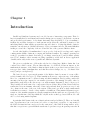
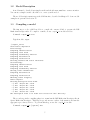
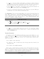
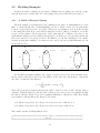
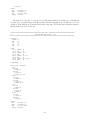
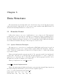
Figure ?? presents an example. The first automaton A(1) has three states x(1) , y (1) , and z (1) ;
the second automaton A(2) has two states x(2) and y (2) . The events of this model are:
• e1 , e2 and e3 : local events involving only A(1) , with constant rates respectively equal to λ1 ,
λ2 and λ3 ;
• e4 : a synchronizing event involving A(1) and A(2) , with a constant rate λ4 ;
• e5 : a local event involving A(2) , with a functional rate f :
f = µ1 , if A(1) is in state x(1) ;
f = 0, if A(1) is in state y (1) ;
f = µ2 , if A(1) is in state z (1) .
When the SAN is in state (z (1) , y (2) ), the event e4 can occur at rate λ4 , and the resulting state
of the SAN can be either (y (1) , x(2) ) with probability π or (x(1) , x(2) ) with probability 1 − π.
e3 , e4 (1 − π)
A(1)
A(2)
x(1)
x(2)
e4 (π)
z (1)
e4
e1
y (2)
y (1)
e5
e2
Figure 2.1: Very Simple SAN model example
We see then that a SAN model is described as a set of automata (each automaton containing
nodes, edges and labels). These may be used to generate the transition matrix of the Markov
chain representing its dynamic behavior using only elementary matrices. This formulation of the
transition matrix is called the SAN descriptor.
4
Chapter 3
Peps Presentation
Peps is software package implemented using the C++ programming language, and although the
source code is quite standard, only Linux and Solaris version have been tested.
The main features of version 2000 are:
• Textual description of continuous-time SAN models (without replicas);
• Stationary solution of models using Arnoldi, GMRES and Power iterative methods [?, ?];
• Numerical optimization regarding functional dependencies, diagonal pre-computation, preconditioning and algebraic aggregation of automata [?]; and
• Results evaluation.
Peps 2003 includes some bug corrections and three new features:
• Compact textual description of continuous-time SAN models;
• Semantic aggregation of SAN with replicas;
• Numerical solution using probability vectors with the size of the reachable state space; and
• Fast(er) function evaluation.
Peps 2007 is able to:
• Read a file which describes a SAN in a textual format, replicas features are improved. This
interface is described in Chapter ??. Section ?? provides simple examples of models that can
be used to experiment with the software.
• Compile a SAN model to form all the small matrices then to assemble them to construct
the complete SAN descriptor. At this level, a choice of granularity is given to the user:
some automata can be grouped to form an equivalent SAN with fewer, but larger automata.
Theses features are described in Chapter ??
• Provide the user with a selection of iterative solution methods to compute stationary and
transient probability vector and a number of numerical options, as it is explained in Chapter
??.
• Inspect data structures such as the reachable state space, the stationary probability vector
(and compare two of them), and the SAN descriptor.
• Output results and data structure files: results, probability vectors, SAN descriptor, HBF
format of the descriptor compatible with the software Marca [?].
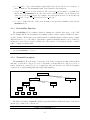
Peps 2007 is composed by some modules. Each module implements a step to a model resolution.
The modules are grouped in three phases: Description, Compiling, and Solution. Description phase
is composed by the interface modules. The data structures modules compose the compiling phase
and the solution phase concerns the solution modules.
The next sections presents a brief description of the steps from to describe a model til to solve
its in the Peps software. Including Peps installation procedures.
3.1
Peps 2007 Installation
Being a academic open-source software, the Peps 2007 installation is quite simple and do not
demand any special feature from your system. The Makefile does not perform any test to verify
the availability of the GNU C++ compiler in the system. This compiler is needed to compile the
Peps software itself during the installation, but also during the execution. Peps 2007 uses the
compilation of functional elements just-in-time [?]. This procedure calls the g++ compiler, so make
sure this command is reachable from your environment (type which g++ at your prompt to verify
it).
3.1.1
Getting the source
Retrieve from our site the file Peps2007.tgz, for full Peps 2007 package or the compressed file
for each individual module. Use tar -xvzf file (e.g. tar -xvzf Peps2007.tgz for full Peps 2007
package) to uncompress this file and to generate the directory Peps2007 and all the hierachy of
files.
3.1.2
Compiling
If you want to compile all Peps 2007 modules, just type make and the binary files of Peps will
be generated. You can compile just one individual module. In this case type make module name
(e.g. make compile san) or run make into module directory. You can change the compiling options
for each module into module directory.
3.1.3
Binary files
In the directory ./bin/ in each module directory there is a file with the module name (e.g.
compile san) which is the executable. To run a Peps module just type the module name. If you
compiled the full Peps 2007 package, all executable files generated by each module are copied to
the directory ./peps2007/bin/. The first time that Peps is running in a directory, it will initialize
all auxiliary subdirectories.
6
3.2
Model Description
A model must be described in a simple text file and the file name must have .san as extention.
You can use a simple text file editor like vi to create your file model.
The model description must respect the SAN interface, described in Chapter ??. Some models
examples are presented in Section ??.
3.3
Compiling a model
The first step to solve a SAN model is to compile the .san model file to generate the Full
Markovian Descriptor files. To compile a .san file, we use compile san module as follow:
Command: compile san file
Typical module output:
./compile_san rs
Start model compilation
First Passage
Compiling identfier block
Compiling event block
Compiling reachability function
Compiling network block
Compiling results block
Creating automata and states structures
Second Passage
Compiling identfier block
Compiling event block
Compiling reachability function
Writing events informations
Compiling network block
Compiling results block
Checking events integrity
Model compiled
Creating description files model
:-) file ’des/rs.des’ saved
:-) file ’des/rs.dic’ saved
:-) file ’des/rs.fct’ saved
:-) file ’des/rs.tft’ saved
:-) file ’des/rs.res’ saved
The description files to rs model were created in "des" directory.
The second step in the compiling phase is to transform the Full Markovian Descriptor files in
Sparse Markovian Descriptor. This step keeps only non-zero values of the matrices and run the
aggregation procedures, if choice. To perform this step, we use the compile dsc module:
Command: compile dsc [options] file
7
Typical using example with standard options:
./compile_dsc rs
Compilation of a SAN model (Internal Descriptor Generation)
Compile_Network
Compile_Function_Table
:-) file ’des/rs.tft’ read
:-) file ’dsc/rs.ftb’ saved
Compile_Descriptor
:-) file ’des/rs.des’ read
:-) file ’dsc/rs.dsc’ saved
Compile_Reacheable_SS
:-) file ’dsc/rs.rss’ saved
:-) file ’des/rs.fct’ read
Compile_Dictionary
:-) file ’dsc/rs.dct’ saved
:-) file ’des/rs.dic’ read
Compile_Integration_Function
:-) file ’des/rs.res’ read
:-) file ’dsc/rs.inf’ saved
Translation performed:
- user time spent:
- system time spent:
- real time spent:
compilation of a SAN model
4.0000000000000001e-03 seconds
0.0000000000000000e+00 seconds
2.7468191855587065e-01 seconds
Thanks for using PEPS!
The last step in the compiling phase is the model normalization. This step normalizes the
Sparse Markovian Descriptor files to Continuous Normalized Descriptor. Two modules can be used
in this step. The norm dsc ex module uses an extended vector format and norm dsc sp module
uses a sparse vector format.
Command: norm dsc ex file or norm dsc sp file
Typical using example output message:
./norm_dsc_ex rs
Normalization of a SAN Descriptor
:-) file ’dsc/rs.rss’ read
:-) file ’dsc/rs.ftb’ read
:-) file ’dsc/rs.dsc’ read
:-) file ’dsc/rs.dct’ read
:-) file ’cnd/rs.cnd’ saved
:-) file ’cnd/rs.ftb’ saved
:-) file ’cnd/rs.rss’ saved
:-) file ’peps/peps2007/bin/jit/peps_jit.C’ saved
8
Translation performed: normalization of a SAN descriptor
(largest element in reachable states: 1.5000000000000000e+01)
- user time spent:
4.0000000000000001e-03 seconds
- system time spent:
4.0000000000000001e-03 seconds
- real time spent:
8.9477301982697099e-01 seconds
Thanks for using PEPS!
3.4
Solving a model
After the compiling phase, the model can be solved. The solution methods are implemented
in two modules, and as in the last compiling step, solve cnd ex module uses an extended vector
format and solve cnd sp module uses a sparse vector format. If you compile your model using the
extended vector, we must use the extended vector representation also to solve its.
Command:solve cnd ex [options] file or solve cnd sp [options] file
Typical using example output message:
./solve_cnd_ex rs
:-) file ’cnd/rs.rss’ read
:-) file ’cnd/rs.ftb’ read
:-) file ’peps/peps2007/bin/jit/peps_jit.C’ saved
:-) file ’cnd/rs.cnd’ read
:-) file ’dsc/rs.dct’ read
Solution of the model ’cnd/rs.cnd’ (4 automata - 11/16 states)
Enter vector file name: v
Iteration 0: largest: 1.6363636363636364e-01 (0) smallest: 5.4545454545454550e-02 (3)
Iteration 10: largest: 2.1944567435636364e-01 (0) smallest: 5.4861419985454539e-02 (3)
Iteration 20: largest: 2.2192409302507105e-01 (0) smallest: 5.5481023256267900e-02 (3)
Iteration 30: largest: 2.2219021084342858e-01 (0) smallest: 5.5547552710857144e-02 (3)
Iteration 40: largest: 2.2221878502659678e-01 (0) smallest: 5.5554696256649189e-02 (3)
Iteration 50: largest: 2.2222185315615217e-01 (0) smallest: 5.5555463289038043e-02 (3)
Iteration 60: largest: 2.2222218259405468e-01 (0) smallest: 5.5555545648513671e-02 (3)
Iteration 70: largest: 2.2222221796718014e-01 (0) smallest: 5.5555554491795035e-02 (3)
Iteration 80: largest: 2.2222222176534054e-01 (0) smallest: 5.5555555441335135e-02 (3)
Iteration 90: largest: 2.2222222217316495e-01 (0) smallest: 5.5555555543291231e-02 (3)
Iteration 91:
Power solution
Number of iterations:
92
- user time spent:
-8.3432745304548583e-20 seconds
- system time spent:
-2.4987471944001860e-19 seconds
- real time spent:
3.4348982153460383e-03 seconds
Residual Error: 7.0642436345025317e-11 - The method converged (solution found)!
:-) file ’v.vct’ saved
9
:-) file ’rs.tim’ saved
Thanks for using PEPS!
10
Part I
PEPS BASIC MODULES
11
Chapter 4
Interface
This chapter presents the SAN textual interface to Peps 2007. This new textual interface is full
compatible with Peps 2003 and incorporates new features to replications sets. Addictionally, we
present some modeling examples to show the interface powerful to model systems based replicated
components.
4.1
SAN Textual Interface
A textual formalism for describing models is proposed, and it keeps the key feature of the SAN
formalism: its modular specification. Peps 2007 incorporates a graph-based approach which is
close to model semantics. In this approach each automaton is represented by a graph, in which
the nodes are the states and the arcs represent transitions fired by the occurrence of events. This
textual description has been kept simple, extensible and flexible.
• Simple because there are few reserved words, just enough to delimit the different levels of
modularity;
• Extensible because the definition of a SAN model is performed hierarchically;
• Flexible because the inclusion of replication structures allows the reuse of identical automata,
and the construction of automata having repeated state blocks with the same behavior, such
as found in queueing models.
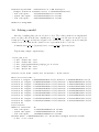
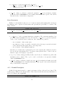
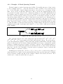
This section describes the Peps 2007 textual formalism used to describe SAN models. To be
compatible with Peps 2007 , any file describing a SAN should have the suffix .san. Figure ??
shows an overview of the Peps input structure. A SAN description is composed of five blocks
(Figure ??) which are easily located with their delimiters1 (in bold). The other reserved words
in the Peps input language are indicated with an italic font. The symbols “<” and “>” indicate
mandatory information to be defined by the user. The symbols “{” and “}” indicate optional
information.
1
The word “delimiters” is used to indicate necessary symbols, having a fixed position in the file.
identifiers
< id name >=< exp > ;
< dom name >= [i..j] ;
events
// without replication
loc < evt name > (< rate >)
syn < evt name > (< rate >)
// with replication
loc < evt name > [replication domain](< rate >)
syn < evt name > [replication domain](< rate >)
{partial} reachability =< exp > ;
network < net name > (< type >)
aut < aut name > {[replication domain]}
stt < stt name > {[replication domain]} {(reward)}
to( < stt name > {[replication domain]} {/f cond} )
< evt name > {[replication domain]} {(< prob >)}
...
< evt name > {[replication domain]} {(< prob >)}
...
from < stt name >
to( < stt name > {[replication domain]} {/f cond} )
< evt name > {[replication domain]} {(< prob >)}
...
stt < stt name > {[replication domain]} {(reward)}
to( < stt name > {[replication domain]} {/f cond} )
< evt name > {[replication domain]} {(< prob >)}
...
aut < aut name > {[replication domain]}
...
{/f cond}
{/f cond}
{/f cond}
{/f cond}
results
;
Figure 4.1: Modular structure of SAN textual format
< res name >=< exp >
4.1.1
Identifiers and Domains
This first block identifiers contains all declarations of parameters: numerical values, functions, or sets of indexes (domains) to be used for replicas in the model definition. An identifier
(< id name >) can be any string of alphanumeric characters. The numerical values and functions
are defined according to a C-like syntax. In general, the expressions are similar to common mathematical expressions, with logical and arithmetic operators. The arguments of these expressions
can be constant input numbers (input parameters of the model), automata identifiers or states
identifiers. In this last case, the expressions are functions defined on the SAN model state space.
For example, “the number of automata in state n0” (which gives an integer result) can be expressed
as “nb n0”. A function that returns the value 4 if two automata (A1 and A2) are in different states,
and the value 0 otherwise, is expressed as “(st A1 ! = st A2) ∗ 4”. Comparison operators return
the value “1” for a true result and the value “0” for a false result. The format of an expression is
described in Section ??.
Format of the identifiers block
identifiers
< id name >=< exp > ;
...
13
< dom name >= [i..j] ;
...
• “< id name >” is an expression identifier which begins with a letter and is followed by
a sequence of letter or numbers. The maximum length of an expression identifier is 128
characters;
• “< dom name >” is a domain identifier. It is a set of indexes. A domain can be defined by
an interval “[1..3]”, by a list “[1,2,3]” or by list of intervals “[1..3,5,7..9]”. Identifiers can be
used to define an interval “[1..ID1,5,7..ID2]”, where ID1 and ID2 are identifiers with constant
values. In all cases, domain must respect an increasing value order;
• “< exp >” is a real number or a mathematical expression. The mathematical expressions are
described in Section ??. A real number has one of the following formats:
an integer, such as “12345”;
a floating point real number, such as “12345.6789”;
a real number with mantissa and exponent, such as “12345E(or e)+(or –)10” or
“12345.6789e+100’.
Sets of indexes are useful for defining numbers of events, automata, or states that can be
described as replications. A group of replicated automata of A with the set in index [0..2, 5, 8..10]
defines the set containing the automata A[0], A[1], A[2], A[5], A[8], A[9], and A[10].
4.1.2
Events
The events block defines each event of the model given
• its type (local or synchronizing);
• its name (an identifier);
• its firing rate (a constant or function previously defined in the identifiers block).
Additionally, events can be replicated using the sets of indexes (domains). This facility can be used
when events with the same rate appear in a set of automata.
Format of the events block
events
loc < evt name > [replication domain](< rate >)
syn < evt name > [replication domain](< rate >)
...
• “loc” define the event type as local event;
• “syn” define the event type as synchronized event;
14
• “< evt name >” the event identifier begins with a letter and is followed by a sequence of
letter or numbers. The maximum length of an identifier is 128 characters;
• “[replication domain]” is a set of indexes. The replication domain must be a domain identifier defined in identifiers block. An event can be replicated til three levels. Each level is
defined by [replication domain]. For example, an event replicated in two levels is defined as
< evt name > [replication domain][replication domain];
• “< rate >” defines the rate of the event. It must be an expression identifier declared in the
identifiers block.
4.1.3
Reachability Function
The reachability block contains a function defining the reachable state space of the SAN
model. Usually, this is a Boolean function, returning a nonzero value for states of Sˆ that belongs to
S. A model where all the states are reachable has the reachability function defined as any constant
different from zero, e.g. , the value 1. Optionally, a partial reachability function can be defined by
adding the reserved word “partial”. In this case, only a subset of S is defined, and the overall S
will be computed by Peps 2007.
Format of the reachability block
{partial} reachability =< exp > ;
4.1.4
Network Description
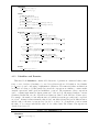
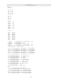
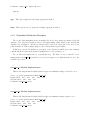
The network block is the major component of the SAN description and has an hierarchical
structure: a network is composed of a set of automata; each automaton is composed of a set of
states; each state is connected to a set of output arcs; and each arc has a set of labels identifying
events (local or synchronizing) that may trigger this transition.
network Example
...
automaton A(1)
...
state 0(1)
...
to 1(1)
evt1
...
evtn
...
...
...
to x(1)
evt1
state x(1)
automaton A(N)
evtn
Figure 4.2: Structure of network hierarchy.
The first level, named “network”, includes general information such as the name of the model
and the type of time scale of the model.
Format of the network block
15
network < net name > (< type >)
aut < aut name > {[replication domain]}
stt < stt name > {[replication domain]} {(reward)}
to( < stt name > {[replication domain]} {/f cond} )
< evt name > {[replication domain]} {(< prob >)} {/f cond}
. . . // Automata description
• “< net name >” is the name of the model. It is a string of alphanumeric characters beginning
with a letter;
• “< type >” is the time scale of the model. Two type are possible: “continuous” or “discrete”.
Currently, only “continuous” model analysis is available in Peps 2007.
The following subsections provide further detail on each of the levels of the network description.
Automaton Description
In this level, each automaton is decribed. The delimiter of the automaton is the reserved word
“aut” and the name of the automaton. Optionally, a domain definition can be used to replicate it,
i.e. , to create a number of copies of this automaton. In this case, if i is a valid index of the defined
domain and A is the name of the replicated automaton, then A[i] is the identifier of one automaton.
Format of the aut block
aut < aut name > {[replication domain]}
stt < stt name > {[replication domain]} {(reward)}
to( < stt name > {[replication domain]} {/f cond} )
< evt name > {[replication domain]} {(< prob >)} {/f cond}
. . . // States description
• “< aut name >” is the name of the automaton. It is an alphanumeric identifier and it may
be used for expression definitions;
• “[replication domain]” is a set of indexes. The replication domain is a domain identifier.
This identifier must defined in identifiers block.
State Description
The stt section defines a local state of the automaton.
Format of the stt block
stt < stt name > {[replication domain]} {(reward)}
to( < stt name > {[replication domain]} {/f cond} )
< evt name > {[replication domain]} {(< prob >)} {/f cond}
. . . // Transitions description
16
• “< stt name >” is the state identifier, which might be used in function evaluation. Peps uses
an internal index for the states for each automaton. The first declared state of an automaton
gets the internal index (also called internal state id) zero, the second gets 1 and so on;
• “[replication domain]” is the number of times that the state appears in the automaton. It
is described by a domain identifier defined in identifiers block;
• “(reward)” is optional and specifies the state reward. When it is not specified, PEPS gives
a default value to the reward, which is the internal state index.
From Description The from section is quite similar to the stt section, but it cannot define local
states. This is commonly used to define additional transitions which cannot be defined in the stt
section. A typical use of the from section is to define a transition leaving from only one state of a
group of replicated states to a state outside the group, e.g. , a queue with particular initial or final
states may need this kind of transition definition.
Format of the from block
from < stt name >
to( < stt name > {[replication domain]} {/f cond} )
< evt name > {[replication domain]} {(< prob >)} {/f cond}
. . . // Transitions description
• “< stt name >” is a state identifier defined in stt section. Use “[x]” after the state identifier
to appoint a specific state in a group of replicated states. “x” must be an identifier previously
defined in identifiers block.
Transition Description
A description of each output transition from this state is given by the definition of a “to()”
section. The identifier “< stt name >” inside the parenthesis indicates the output state of this
transition. “[x]” can be used to appoint to a specific or a set of replicated states. In this case, three
situation are possibles:
• use a constant to define a static state;
• use a function to define one variable state, where the target state index is defined by the
current state index;
• use a domain to define multiply transitions.
Inside a group of replicated states, the expression of the other states inside the group can be
made by positional references to the current (==), the previous (– –) or the successor (++). Larger
jumps, e.g. , of states two ahead (+2), can also be defined, but any positional reference pointing
to a non-existing state or to a state outside the replicated group is ignored.
Format of the to block
17
to( < stt name > {[replication domain]} {/f cond} )
< evt name > {[replication domain]} {(< prob >)} {/f cond}
. . . // Events description
• “/f cond” defines a condition to include the transition. f cond is an function identifier
previously defined in identifiers block. Normally, this function value depend of the current
automaton and/or current and/or target state.
Event Description
Finally, for each transition defined, a set of events (local and synchronizing) that can triggers
the transition can be expressed by their names and optionally the probability of occurrence, and
firing condition.
Format of the event block
< evt name > {[replication domain]} {(< prob >)} {/f cond}
• “< evt name >” is the event name that trigger a transition. The event name must have been
previously defined in events block. Use “[x]” after the < evt name > to specify a replicated
event or a set of replicated states. In this case, three situation are possibles:
– use a constant to define a static state;
– use a function to define one variable event index, where the target event index is defined
by the current automaton/state index or the target state;
– use a domain to define multiply transitions.
Remember, we can have three replications level for each event, the three situations described
here are able in each replication level. To address events replicated in two or three levels you
must use “[x][x]” and “[x][x][x]”, respectively;
• “(< prob >)” is the routing probability for this event. If only one destination is possible, this
information can be omitted. The < prob > can be a real value or an expression identifier
defined in identifiers block;
• “/f cond” defines a condition to include an event. f cond is an function identifier previously
defined in identifiers block. Normally, this function value depend of the current automaton
and/or current and/or target state.
4.1.5
Results Description
In this block, the functions used to compute performance indexes of the model are defined. The
results given by PEPS are the integral values of these functions with the stationary distribution of
the model. This module is optional.
Format of the results block
18
results
< res name >=< exp > ;
• < res name > is a single identifier;
• < exp > is a mathematical expression. The mathematical expressions are described in Section
??.
4.1.6
Function Expressions
This section presents the possibilities that PEPS provides to build expressions and functions.
In general, the expressions are similar to common mathematical expressions, with logical and
arithmetic operators. The arguments of these expressions can be constant input numbers, but can
also be automata or states identifiers.
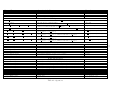
The format of the operators is summarized in table ??. The internal format used in PEPS
solver is given in the fourth column, and it is useful only when debugging PEPS. The arithmetic
operators are “+”, “−”, “∗”, “/”, “div”, “mod”, “max” and “min” and are not typed (integer or
real values). PEPS expressions do not have operators priorities and are evaluated from the left to
the right. To specify priorities, it is necessary to use brackets. For example, 5 + 6 ∗ 7 is computed
as (5 + 6) ∗ 7 in PEPS.
The relational operators are “==”, “! =”, “<”, “>”, “<=”, “>=”. Their result is 1 (coding
for TRUE) if the relation is verified and 0 (coding for FALSE) otherwise. The logical operators
are: “not” coded with “!”, “or” with “||”, “and” with “&&”, “XOR” with ∧.
As we already mentioned, the arguments of these operators can be constant values (input of
the model), but also functions of the SAN state. We can have two kind of functions. The first one
is called “description functions” and the second one is “SAN functions”.
Description Functions
Description functions are used in the model description and they are useful to replicate states,
transitions, and events. When Peps 2007 genere the Markovian Descriptor (set of matrices that
describe the model), it take in to account these functions to build the model.
Peps 2007 defines three functions:
• at : returns the current automaton index. If automaton is a replicated automaton then this
function returns the internal replication index else it returns the general automaton index in
the model;
• sts : gives the current state index in the current automaton. As well the previous functions,
this functions returns the internal replication index to a replicated state and the general state
index to a non replicated state;
• std : this functions returns the target state in a transition. The states indexes returned by
this functions follow the previous functions behaviour.
19
SAN Functions
With the idea that a SAN has a state which evolves with time, we use the term “current state”.
These functions are used to express SAN behavior such as “the rate of this event is 0 if the SAN is
in state x and equal to r otherwise”, or to compute performance index by integration of a function
such as “the number of automata in state 0”. Before proceeding to these functions, let us describe
the way names (identifiers) are handled in PEPS.
• a reference to an automaton identifier is translated in PEPS into a reference to the automaton
internal index. This internal index is computed according to the declaration order in the
Network block. The first automaton of the network has internal index zero, the second 1
and so on. Replicated automata are internally numbered using the index of the first one as a
base and then incrementing it with the replication index. For example, assume a SAN with
automaton test1 replicated in the interval [1..2], automaton test2 without replication
and automaton test3 replicated 3 times ([0..2]) , then we have the external identifiers:
test1[1], test1[2], test2, test3[0], test3[1] and test3[2]. The internal indexes are: 0 for
test1[1], 1 for test1[2], 2 for test2, 3 for test3[0], 4 for test3[1] and 5 for test3[2]. This
internal numbering allows to defined subsets of automata as intervals. The interval (test1[2],
test3[1]) is exactly the subset of automata: test1[2], test2, test3[0], test3[1].
• a reference to a state identifier is also replaced in PEPS with a reference to an automaton
index. The external identifiers correspond to an internal index computed according to the
declaration order and the number of replications. For example, if the automaton test1 has 3
states, named A, B and C declared in this order, the internal index of A is 0, B is 1 and C
is 2. If there are replications, the corresponding offset is applied. For a single queue, a state
is replicated, and it works as follows: take a queue with a block of replicated states. This
block has one state rep replicated four times. Then, the internal index ranges from 0 to 3 in
the order : rep[0], rep[1], rep[2], and rep[3], but the first rep[0] and the last rep[3] have
some transitions to outside the group ignored.
• Peps maintains a global (for all the automata) table giving a correspondence between a
state external identifier and state internal index (called name-index table). If several distinct
automata have the same state identifier, a warning is output if and only if these states do not
have the same internal index. This situation might lead to errors if these state identifiers do
not correspond to the same internal index (internal indexes are computed per automaton).
So the user should be aware of this implementation when writing a function based on external
identifiers as “number of automata in state n0”.
These functions are:
• st < aut name > : gives the current state of automaton < aut name >. < aut name >
is an external identifier, and the output of this function is an internal state index. Another
(historical) syntax for this function is @ < aut name >.
• nb < stt name > : gives the total number of automata of the SAN in the state < stt name >.
< stt name > is an external identifier and Peps translates it into an internal index. The user
should be careful when using this function: it might lead to errors when there are automata
having a state named < stt name > but with different internal index, or when there are
automata without a state named < stt name > (PEPS gives a warning in this case).
20
• nb [< aut name > .. < aut name >] < stt name > : it is an extension of the preceding
function, but the count is done on the automata interval [< aut name > .. < aut name >].
The notion of “interval” refers to the total ordering described above. This notation is very
useful when an automaton is replicated and the interval is exactly all the replicated automata.
• rw < aut name > : in SAN, rewards may be associated to states. This function gives the
current reward of automaton < aut name >. < aut name > is an external identifier, and the
output of this function is a reward, thus a real or integer value. This function is very similar
to st < aut name >. Remember that if the reward is not explicitly given by the user, the
internal state index is used as a reward. This makes sense when the states coded 0, 1, 2, etc.
are the number of customers in a queue. In this case the two functions rw < aut name >
and st < aut name > are identical.
• sum rw [< aut name > .. < aut name >] : gives the sum of the current rewards of the
automata in the interval [aut name > .. < aut name >].
• sum rw [< aut name > .. < aut name >] < stt name > : gives the sum of the rewards
of the automata in the interval [< aut name > .. < aut name >) which are in the state
< stt name >.
• prod rw [< aut name > .. < aut name >] and
prod rw [< aut name > .. < aut name >] < stt name >: are similar to the preceding
functions, with a change of operator.
External Format
Semantic of the Format
Description Operators
Example
at
sts
std
gives the current automaton index
gives the current state index
gives the target state index
at
sts
std
st < aut name >
@ < aut name >
nb < stt name >
nb [< aut name > .. < aut name >] < stt name >
gives the current state of automaton “< aut name >”
the same as above, another notation
gives the total number of automata in the state “< stt name >”
for the automata in the interval “[< aut name > .. < aut name >]”, gives the total
number of automata in the state “< stt name >”
gives the reward associated with the current state of automaton “< aut name >”
gives the sum of the rewards of the current states of the automata in the interval
[< aut name > .. < aut name >]
gives the sum of the rewards of the automata in the interval
“< aut name > .. < aut name >”, which are in the state < stt name >
product of the rewards of the current of the automata of interval
“< aut name > .. < aut name >”
product of the rewards of the current states of the automata of interval
“< aut name > .. < aut name >”, which are in the state < stt name >
SAN Operators
rw < aut name >
sum rw [< aut name > .. < aut name >]
sum rw [< aut name > .. < aut name >] < stt name >
prod rw [< aut name > .. < aut name >]
prod rw [< aut name > .. < aut name >]< stt name >
st processA
@processA
nb util
nb [processA .. processD) util
rw processA
sum rw [processA .. processD]
sum rw [processA .. processD] util
prod rw [processA .. processD]
product rw [processA .. processD] util
sum of “< exp1 >” and “< exp2 >”
substraction of “< exp2 >”minus “< exp1 >”
product of “< exp1 >” and “< exp2 >”
5 + 3
5 − 3
5 ∗ 3
min ( < exp1 >, < exp2 >]
max ( < exp1 >, < exp2 >]
division of “< exp1 >” by “< exp2 >”
integer division of “< exp1 >” and “< exp2 >”
rest of integer division of “< exp1 >” by “< exp2 >”
gives the miniimum of two arguments
gives the maximum of two arguments
5/3
5 div 3
5 mod 3
min(5,3)
max(5,3)
Relational Operators
< exp1 >
< exp1 >
< exp1 >
< exp1 >
< exp1 >
< exp1 >
== < exp2 >
! = < exp2 >
< < exp2 >
<= < exp2 >
> < exp2 >
>= < exp2 >
if
if
if
if
if
if
“<
“<
“<
“<
“<
“<
exp1 >”
exp1 >”
exp1 >”
exp1 >”
exp1 >”
exp1 >”
is
is
is
is
is
is
equal to “< exp2 >”, gives true (“1”) else false (“0”)
not equal to “< exp2 >”, givess true (“1”) else false (“0”)
smaller than “< exp2 >”, gives true (“1”) else false (“0”)
smaller or equal than “< exp2 >”, gives true (“1”) else false (“0”)
greather than “< exp2 >”, results true (“1”) else results false (“0”)
greater or equal than “< exp2 >”, gives true (“1”) else false (“0”)
5
5
5
5
5
5
== 3
!= 3
< 3
<= 3
> 3
>= 3
Logical Operators
! < exp >
< exp1 >
< exp1 >
< exp1 >
|| < exp2 >
&& < exp2 >
∧ < exp2 >
logical “not”
5 > 3) ! (7 < 8)
logical “or”
logical “and”
logical “XOR”
(5 > 3) || (7 < 8)
(5 > 3) && (7 < 8)
(5 > 3) ∧ (7 < 8)
Table 4.1: Operators
22
Arithmetic Operators
+ < exp2 >
− < exp2 >
∗ < exp2 >
< exp1 > / < exp2 >
< exp1 > div < exp2 >
< exp1 > mod < exp2 >
< exp1 >
< exp1 >
< exp1 >
4.2
Modeling Examples
In this section three examples are presented to illustrate the modeling power and the computational effectiveness of Peps 2007. For each example, the generic SAN model is described.
4.2.1
A Model of Resource Sharing
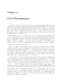
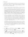
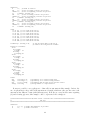
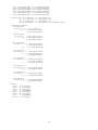
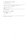
The first example is a traditional resource sharing model, where N distinguishable processes
share a certain amount (R) of indistinguishable resources. Each of these processes alternates
between a sleeping and a resource using state. When a process wishing to move from the sleeping
to the using state finds R processes already using the resources, that process fails to access the
resource and it returns to the sleeping state. Notice that when R = 1 this model reduces to the
usual mutual exclusion problem. Analogously, when R = N all the processes are independent and
there is no restriction to access the resources. We shall let λi be the rate at which process i awakes
from the sleeping state wishing to access the resource, and µi , the rate at which this same process
releases the resource.
A(1)
sleeping
R1
sleeping
• • •
R2
sleeping
RN
G1
using
A(N )
A(2)
G2
GN
• • •
using
using
Figure 4.3: Resource Sharing Model - version 1
In our SAN representation (Figure ??), each process is modeled by a two state automaton A(i) ,
the two states being sleeping and using. We shall let stA(i) denote the current state of automaton
A(i) . Also, we introduce the function
f =δ
N
X
δ(stA
(i)
i=1
!
= using) < R .
where δ(b) is an integer function that has the value 1 if the Boolean b is true, and the value 0
otherwise. Thus the function f has the value 1 when access to the resource is permitted and has
the value 0 otherwise. Figure ?? provides a graphical illustration of this model, called RS1. In this
representation each automaton A(i) has two local events:
• Gi which corresponds to the i-th process getting a resource, with rate λi f ;
• Ri which corresponds to the i-th process releasing a resource, with rate µi .
The textual .san file describing this model is:
//========================================== RS model version 1 =======================================
//
N=4, R=2
//=====================================================================================================
23
identifiers
R
=
mu1
=
lambda1 =
f1
=
mu2
=
lambda2 =
f2
=
mu3
=
lambda3 =
f3
=
mu4
=
lambda4 =
f4
=
events
loc
loc
loc
loc
loc
loc
loc
loc
G1
R1
G2
R2
G3
R3
G4
R4
2;
//
6;
//
3;
//
lambda1
5;
//
4;
//
lambda2
4;
//
6;
//
lambda3
3;
//
5;
//
lambda4
(f1)
(mu1)
(f2)
(mu2)
(f3)
(mu3)
(f4)
(mu4)
//
//
//
//
//
//
//
//
amount of resources
rate for leaving a resource for process 1
rate for requesting a resource for process
* (nb using < R);
rate for leaving a resource for process 2
rate for requesting a resource for process
* (nb using < R);
rate for leaving a resource for process 3
rate for requesting a resource for process
* (nb using < R);
rate for leaving a resource for process 4
rate for requesting a resource for process
* (nb using < R);
local
local
local
local
local
local
local
local
event
event
event
event
event
event
event
event
G1
R1
G2
R2
G3
R3
G4
R4
reachability = (nb using <= R);
has
has
has
has
has
has
has
has
rate
rate
rate
rate
rate
rate
rate
rate
1
2
3
4
f1
mu1
f2
mu2
f3
mu3
f4
mu4
// only the states where at the most R
// resources are being used are reachable
network rs1 (continuous)
aut P1
stt sleeping
to(using)
G1
stt using
to(sleeping) R1
aut P2
stt sleeping
to(using)
G2
stt using
to(sleeping) R2
aut P3
stt sleeping
to(using)
G3
stt using
to(sleeping) R3
aut P4
stt sleeping
to(using)
G4
stt using
to(sleeping) R4
results
full
empty
use1
average
=
=
=
=
nb
nb
st
nb
using == R;
using == 0;
P1 == using;
using;
//
//
//
//
probability of all resources being used
probability of all resources being available
probability that the first process uses the resource
average number of occupied resources
It was not possible to use replicators to define all four automata in this example. In fact, the
use of replications is only possible if all automata are identical, which is not the case here since each
automaton has different events (with different rates). If all the processes had the same acquiring
(λ) and releasing (µ) rates, this example could be represented more simply as:
//================================ RS model version 1 with same rates =================================
//
N=4, R=2
//=====================================================================================================
identifiers
N
= [0..3];
R
= 2;
// amount (and identifier) of processes
// amount of resources
24
mu
lambda
i
f
=
=
=
=
6;
3;
at;
lambda *
events
loc Acq[N] (f)
loc Rel[N] (mu)
// rate for leaving a resource for all processes
// rate for requesting a resource for all processes
// current automaton index
(nb using < R);
// local events Acq have rate f
// local events Rel have rate mu
reachability = (nb using <= R);
// only the states where at the most R
// resources are being used are reachable
network rs1 (continuous)
aut P[N]
stt sleeping
to(using)
Acq[i]
stt using
to(sleeping) Rel[i]
results
full
empty
use1
average
=
=
=
=
nb
nb
st
nb
using == R;
using == 0;
P[0] == using;
using;
//
//
//
//
probability of all resources being used
probability of all resources being available
probability that the first process uses the resource
average number of occupied resources
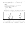
We wish to point out that in the Peps documentation, a number of variants of this model are
included, to show that it is possible with only simple modifications to introduce a complete set of
related models. Within the scope of this manual, it is interesting to describe a specific variation of
this model that describes exactly the same problem, but which does not use functions to represent
the resource contention. In fact, in this case, and in many others, synchronizing events can be used
to generate an equivalent model without functional rates (freqeuntly with many more automata,
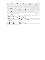
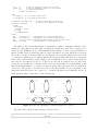
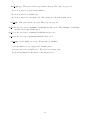
states, and/or synchronizing events). Figure ?? presents this new model, where an automaton is
introduced to represent the resource pool. The resource allocation (events Gi , rate λi ) and release
(events Ri , rate µi ) that were formerly described as local events, will now be synchronizing events
that increment the number of occupied resources at each possible allocation, and decrement it at
each release. The resource contention is modeled by the impossibility of a process passing to the
using state when all resources are occupied, i.e. , when the automaton representing the resource is
in the last state (where only release events can happen).
A(1)
sleeping
• • •
sleeping
R2
R1
sleeping
RN
GN
G2
G1
• • •
using
using
G1 , G2 , . . . , GN
A(N +1)
A(N )
A(2)
0
G1 , G2 , . . . , GN
1
• • •
2
using
G1 , G2 , . . . , GN
R
• • •
R1 , R2 , . . . , RN
R1 , R2 , . . . , RN
R1 , R2 , . . . , RN
Figure 4.4: Resource Sharing Model without functions - version 2
The Peps 2003 textual format of this model is as follows:
//========================================== RS model version 2 =======================================
//
N=4, R=2
//=====================================================================================================
25
identifiers
R
mu1
lambda1
mu2
lambda2
mu3
lambda3
mu4
lambda4
res_pool
events
syn
syn
syn
syn
syn
syn
syn
syn
G1
R1
G2
R2
G3
R3
G4
R4
=
=
=
=
=
=
=
=
=
=
2;
6;
3;
5;
4;
4;
6;
3;
5;
[0..R];
(f1)
(mu1)
(f2)
(mu2)
(f3)
(mu3)
(f4)
(mu4)
P1
P1
P2
P2
P3
P3
P4
P4
RP
RP
RP
RP
RP
RP
RP
RP
//
//
//
//
//
//
//
//
//
//
amount of resources
rate for leaving a resource for process 1
rate for requesting a resource for process
rate for leaving a resource for process 2
rate for requesting a resource for process
rate for leaving a resource for process 3
rate for requesting a resource for process
rate for leaving a resource for process 4
rate for requesting a resource for process
domain to describe the available resources
//
//
//
//
//
//
//
//
event
event
event
event
event
event
event
event
G1
R1
G2
R2
G3
R3
G4
R4
has
has
has
has
has
has
has
has
rate
rate
rate
rate
rate
rate
rate
rate
1
2
3
4
pool
f1 and appears in automata P1 and RP
mu1 and appears in automata P1 and RP
f2 and appears in automata P2 and RP
mu2 and appears in automata P2 and RP
f3 and appears in automata P3 and RP
mu3 and appears in automata P3 and RP
f4 and appears in automata P4 and RP
mu4 and appears in automata P4 and RP
reachability = (nb [P1..P4] using == st RP);
// the number of Processes using resources must be equal to number
// of occupied resources in the Resource Pool
network rs2 (continuous)
aut P1
stt sleeping
to(using)
G1
stt using
to(sleeping) R1
aut P2
stt sleeping
to(using)
G2
stt using
to(sleeping) R2
aut P3
stt sleeping
to(using)
G3
stt using
to(sleeping) R3
aut P4
stt sleeping
to(using)
G4
stt using
to(sleeping) R4
aut RP
stt n[res_pool]
to(++) G1 G2 G3 G4
to(--) R1 R2 R3 R4
results
full
empty
use1
average
4.2.2
=
=
=
=
st
st
st
st
RP == n[R];
RP == n[0];
P1 == using;
RP;
//
//
//
//
probability of
probability of
probability of
average number
all resources being used
all resources being available
the first process use the resource
of occupied resources
First Server Available Queue
The second example considers a queue with common exponential arrival and a finite number
(C) of distinguishable and ordered servers (Ci , i = 1 . . . C). As a client arrives, it is served by the
first available server, i.e. , if C1 is available, the client is served by it, otherwise if C2 is available
the client is served by it, and so on. This queue behavior is not monotonic, so, as far as we can
ascertain, there is no product-form solution for this model. The SAN model describing this queue
26
is presented in Figure ??. The basic technique to model this queue is to consider each server as a
two-state automaton (states idle and busy). The arrival in each server is expressed by a local event
(called Li ) with a functional rate that is nonzero and equal to λ, if all preceding servers are busy,
and zero otherwise. At a given moment, only one server, the first available, has a nonzero arrival
rate. The end of service at each server is simply a local event (Di ) with constant rate µi .
A(1)
A(2)
idle
D1
idle
• • •
D2
L1
busy
A(C)
idle
DC
L2
LC
• • •
busy
busy
Figure 4.5: First Server Available Model
The Peps 2007 textual formats for this model is as follows:
//================================================ FSA model ==========================================
//
(with functions)
C=4
//=====================================================================================================
identifiers
lambda =
mu1
=
f1
=
mu2
=
f2
=
mu3
=
f3
=
mu4
=
f4
=
events
loc
loc
loc
loc
loc
loc
loc
loc
L1
D1
L2
D2
L3
D3
L4
D4
5;
6;
lambda;
5;
(st C1 == busy) * lambda;
4;
(nb[C1..C2] busy == 2) * lambda;
3;
(nb[C1..C3] busy == 3) * lambda;
(f1)
(mu1)
(f2)
(mu2)
(f3)
(mu3)
(f4)
(mu4)
reachability = 1;
network fsa (continuous)
aut C1
stt idle
to(busy) L1
stt busy
to(idle) D1
aut C2
stt idle
to(busy) L2
stt busy
to(idle) D2
aut C3
stt idle
to(busy) L3
stt busy
to(idle) D3
aut C4
stt idle
to(busy) L4
stt busy
27
to(idle) D4
results
full
empty
use1
average
=
=
=
=
nb
nb
st
nb
busy == C;
busy == 0;
P1 == busy;
busy;
The same model can also be expressed as a SAN without functions. In this case, each function
is replaced by a synchronizing event that synchronizes the automaton representing the server accepting a client with all previous automata in the busy state. The Peps 2003 textual formats for
this alternative model is as follows:
//================================================ FSA model ==========================================
//
(with synchronizing events)
C=4
//=====================================================================================================
identifiers
lambda =
mu1
=
mu2
=
mu3
=
mu4
=
events
loc
loc
syn
loc
syn
loc
syn
loc
L1
D1
L2
D2
L3
D3
L4
D4
5;
6;
5;
4;
3;
(lambda)
(mu1)
(lambda)
(mu2)
(lambda)
(mu3)
(lambda)
(mu4)
C1
C1
C1 C2
C1
C1 C2 C3
C3
C1 C2 C3 C4
C4
reachability = 1;
network fsa2 (continuous)
aut C1
stt idle
to(busy) L1
stt busy
to(idle) D1
to(busy) L2 L3 L4
aut C2
stt idle
to(busy) L2
stt busy
to(idle) D2
to(busy) L3 L4
aut C3
stt idle
to(busy) L3
stt busy
to(idle) D3
to(busy) L4
aut C4
stt idle
to(busy) L4
stt busy
to(idle) D4
results
full
empty
use1
average
=
=
=
=
nb
nb
st
nb
busy == C;
busy == 0;
P1 == busy;
busy;
28
4.2.3
Example: A Mixed Queueing Network
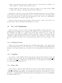
The final example is a mixed queueing network (Fig. ??) in which customers of class 1 arrive
to and eventually depart (i.e., open) and customers of class 2 circulate forever in the network,
(i.e., closed). This quite complex example is presented to stress the power of description of Peps
2003 , and to provide a really large SAN model. Due to its size, the equivalent SAN model is
not presented as a figure. However, the construction technique does not differ significantly from
the technique employed with the previous models. In this model, each queue visited by only the
1
1
first class of customer (Queues 2 and 3) is represented by one automaton each (A(2 ) and A(3 ) ,
respectively). Queues visited by two classes of customers are represented by two automata (one for
each class) and the total number of customers in a queue is the sum of customers (of both classes)
represented in each automaton. The size of this model depends on the maximum capacity of each
queue, denoted Ki for queue i. For the second class of customer (closed system) it is also necessary
to define the number of customers in the system (N2 ). In this example, all queues block when the
destination queue is full, even though other behavior, e.g. , loss, could be easily modeled with the
SAN formalism.
π3
π1
2
1
π6
π2
4
π4
π5
3
5
Figure 4.6: Mixed queueing network
1
2
1
1
The equivalent SAN model for this example has eight automata (A(1 ) , A(1 ) , A(2 ) , A(3 ) ,
2
1
2
A , A(4 ) , A(5 ) , A(5 ) ) representing each possible pair (customer, queue). The model has two
local events (arrival and departure of class 1 customers), and nine synchronizing events (the routing
paths for customers from both classes). Functional transitions are used to represent the capacity
restriction of admission in queues accepting both classes of customer. The reachability function of
the SAN model representing this queueing network must take into account both the unreachable
states due to the use of two automata to represent a queue accepting two classes of customer and
the fixed number of customers of class 2.
(41 )
Assuming queue capacities K1 = 10, K2 = 5, K3 = 5, K4 = 8, K5 = 8, and a total population of
class 2 customers, N2 , equal to 10, the equivalent SAN model has a product state space containing
28, 579, 716 states of which only 402, 732 are reachable. This model is described as follow. More
detailes can be obtained from the Peps web page [?].
29
//================================================ MQN model ==========================================
//
Mixed Queueing Network
//=====================================================================================================
identifiers
N2 = 10;
K1
K2
K3
K4
K5
=
=
=
=
=
[0..10];
[0..5];
[0..5];
[0..8];
[0..8];
k1
k2
k3
k4
k5
=
=
=
=
=
10;
5;
5;
8;
8;
Sri00
Sri01
Sri02
Sri03
Sri04
Sri10
Sri13
Sri14
=
=
=
=
=
=
=
=
Lri00 =
Mu00
Mu01
Mu02
Mu03
Mu04
Mu10
Mu13
Mu14
=
=
=
=
=
=
=
=
0.1;
0.2;
0.3;
0.4;
0.5;
0.1;
0.4;
0.5;
1;
1/Sri00;
1/Sri01;
1/Sri02;
1/Sri03;
1/Sri04;
1/Sri10;
1/Sri13;
1/Sri14;
F_queue1 =
( st class1_queue1 + st class2_queue1 ) < k1;
F_queue2 =
( st class1_queue2 ) < k2;
F_queue3 =
( st class1_queue3 ) < k3;
F_queue4 =
( st class1_queue4 + st class2_queue4 ) < k4;
F_queue5 =
( st class1_queue5 + st class2_queue5 ) < k5;
FL_class1_queue1 =
Lri00 * F_queue1;
n1_c1
n1_c2
n4_c1
n4_c2
n5_c1
n5_c2
=
=
=
=
=
=
st
st
st
st
st
st
class1_queue1/(st
class2_queue1/(st
class1_queue4/(st
class2_queue4/(st
class1_queue5/(st
class2_queue5/(st
rot_class1_queue1toqueue2
rot_class1_queue1toqueue4
rot_class1_queue2toqueue3
rot_class1_queue2toqueue5
rot_class1_queue4toqueue3
rot_class1_queue4toqueue5
rot_class2_queue1toqueue4
rot_class2_queue4toqueue5
rot_class2_queue5toqueue1
rot_class1_queue3toOUT =
rot_class1_queue5toOUT =
=
=
=
=
=
=
=
=
=
class1_queue1
class1_queue1
class1_queue4
class1_queue4
class1_queue5
class1_queue5
+
+
+
+
+
+
st
st
st
st
st
st
class2_queue1);
class2_queue1);
class2_queue4);
class2_queue4);
class2_queue5);
class2_queue5);
0.5 * Mu00 * n1_c1;
0.5 * Mu00 * n1_c1;
0.5 * Mu01;
0.5 * Mu01;
0.5 * Mu03 * n4_c1;
0.5 * Mu03 * n4_c1;
1 * Mu10 * n1_c2;
1 * Mu13 * n4_c2;
1 * Mu14 * n5_c2;
Mu02;
Mu04 * n5_c1;
events
loc l_FL_class1_queue1 (FL_class1_queue1)
loc l_rot_class1_queue3toOUT (rot_class1_queue3toOUT)
loc l_rot_class1_queue5toOUT (rot_class1_queue5toOUT)
syn s_class1_queue1toqueue2 (rot_class1_queue1toqueue2)
syn s_class1_queue1toqueue4 (rot_class1_queue1toqueue4)
syn s_class1_queue2toqueue3 (rot_class1_queue2toqueue3)
30
syn
syn
syn
syn
syn
syn
s_class1_queue2toqueue5
s_class1_queue4toqueue3
s_class1_queue4toqueue5
s_class2_queue1toqueue4
s_class2_queue4toqueue5
s_class2_queue5toqueue1
reachability =
&&
&&
&&
((st
((st
((st
((st
(rot_class1_queue2toqueue5)
(rot_class1_queue4toqueue3)
(rot_class1_queue4toqueue5)
(rot_class2_queue1toqueue4)
(rot_class2_queue4toqueue5)
(rot_class2_queue5toqueue1)
class1_queue1
class1_queue4
class1_queue5
class2_queue1
+
+
+
+
st
st
st
st
class2_queue1)<= k1)
class2_queue4)<= k4)
class2_queue5)<= k5)
class2_queue4 + st class2_queue5) == N2);
network mqn (continuous)
aut class1_queue1
stt n[K1] to(++) l_FL_class1_queue1
to(--) s_class1_queue1toqueue2
s_class1_queue1toqueue4
aut class1_queue2
stt n[K2] to(++)
to(--)
aut class1_queue3
stt n[K3] to(++)
to(--)
aut class1_queue4
stt n[K4] to (++)
to (--)
aut class1_queue5
stt n[K5] to (++)
to (--)
s_class1_queue1toqueue2
s_class1_queue2toqueue3
s_class1_queue2toqueue5
s_class1_queue2toqueue3
s_class1_queue4toqueue3
l_rot_class1_queue3toOUT
s_class1_queue1toqueue4
s_class1_queue4toqueue3
s_class1_queue4toqueue5
s_class1_queue2toqueue5
s_class1_queue4toqueue5
l_rot_class1_queue5toOUT
aut class2_queue1
stt n[K1] to (++)
to (--)
s_class2_queue5toqueue1
s_class2_queue1toqueue4
aut class2_queue4
stt n[K4] to (++)
to (--)
s_class2_queue1toqueue4
s_class2_queue4toqueue5
aut class2_queue5
stt n[K5] to (++)
to (--)
s_class2_queue4toqueue5
s_class2_queue5toqueue1
results
nri00
nri01
nri02
nri03
nri04
nri10
nri13
nri14
=
=
=
=
=
=
=
=
st
st
st
st
st
st
st
st
class1_queue1;
class1_queue2;
class1_queue3;
class1_queue4;
class1_queue5;
class2_queue1;
class2_queue4;
class2_queue5;
31
Chapter 5
Data Structure
The data structures used in Peps 2007 can be divided in two large blocks. The first block uses
a Kronecker (tensor) format and the second one uses a sparse matrix format (HBF). Each block
and theirs modules implementation are described below.
5.1
Kronecker Format
In Kronecker format, we use a set of small matrices to store a large model. This structured
format allows to save storage space in comparison to non-structured format. Compiling phase for
kronecker structures is composed by two step. The first one transforms a Full Markovian Descriptor
in a Sparse Markovian Descriptor and the second one transforms a Sparse Markovian Descriptor
in a Continuous Normalized Descriptor. Theses steps are described below.
5.1.1
Sparse Markovian Descriptor
The first step is to convert the set of small matrices (Full Markovian Descriptor) created in
SANcompilation module in a set of sparse matrices (Sparse Markovian Descriptor). This procedure converts the textual matrices format used in descrption phase to a Peps 2007 internal
representation format.
This step also implements the aggregation methods. Two aggregation methods are implemented
in Peps 2007 . The first one does an algebrique automata aggregation, i.e. tensor operation are
applied in a set of automata. The second method applies a replicas aggregation methods. More
informations about theses techniques can be find in [?].
This step is implemented in compile dsc module.
compile dsc Module Implementation
This module implements the Markovian Descriptor generation in the internal Peps format from
the standard input (textual matrices generated in .san compilation phase).
Source code path: peps2007/src/ds/compile dsc
Required files: .des, .dic, .fct, .tft, .res
Generated files: .dsc, .dct, .ftb, .inf, .rss
Command: compile dsc [options] file
Options:
aggr This option applies the algebrique aggregation method.
lump
This option is used to apply the semantic aggregation method.
5.1.2
Normalized Markovian Descriptor
The second data manipulation step normalizes the model and extract the matrices diagonal
elements. The diagonal generation removes all synchronizing adjust matrices and all diagonal
elements in local matrices. All theses elements will be placed in a diagonal vector used by the
solutions methods. This technique improves the solution methods performance.
In this step, some model analisys are performed, as product and reachable space state analysis,
constant functions replacement, matrices multiplication order generation, etc.
Two modules was implemented to perform this step. The first one uses a extended vector
implementation (norm dsc ex) and the second one uses a sparse vector implementation to store the
reachable space state.
norm dsc ex Module Implementation
This module implements the Markovian Description normalization using a extended vector.
Source code path: peps2007/src/ds/norm dsc ex
Required files: .dsc, .dct, .ftb, .inf, .rss
Generated files: .cnd, .ftb, .rss
Command: norm dsc ex file
norm dsc sp Module Implementation
This module implements the Markovian Description normalization using a sparse vector.
Source code path: peps2007/src/ds/norm dsc sp
Required files: .dsc, .dct, .ftb, .inf, .rss
Generated files: .cnd, .ftb, .rss
Command: norm dsc sp file
5.2
5.2.1
Harwell-Boeing Format (HBF)
HBF Generation
This module performs the equivalent Markov Chain generation from the SAN model. This
Markov Chain represented by a transition matrix is stored in HBF format.
This generation is implemented in gen hbf module..
gen hbf Module Implementation
This module implements the equivalent markovian model (in hbf format) generator from the
SAN Markovian Descriptor.
Source code path: peps2007/src/ds/gen hbf
Required files: .dsc, .dct, .ftb, .inf, .rss
Generated files: .hbf
Command: gen hbf [option] file
Option:
conv This option converte the sparse matrix generated by Peps (C language) in a sparse matrix
in MARCA pattern (Fortran language).
34
Chapter 6
Solution Methods
Peps 2007 implements two sets of methods to analytical solutions of a SAN model. The first
set works with a kronecker format and the second set works with a sparse format (HBF).
6.1
6.1.1
Kronecker Format
Shuffle
The shuffle method basic idea is multiply the probability vector by the set of matrices that
compose the Markovian Descriptor. In fact, each small matrix multiplies a part of the vector. The
sum of all small matrices multiplication is a complete vector-descriptor multiplication.
This multiplication method was implemented in two versions. The first one works with extended
vector (with the global espace state size). The second one works with sparse vector (only the
reachable space state size).
solve cnd ex Module Implementation
This module implements the solution methods using an extended vector.
Source code path: peps2007/src/solve/solve cnd ex
Required files: .cnd, .ftb, .rss, .inf, .dct
Generated files: .vct, .tim
Command:solve cnd ex [options] file
solve cnd sp Module Implementation
This module implements the solution methods using a sparse vector.
Source code path: peps2007/src/solve/solve cnd sp
Required files: .cnd, .ftb, .rss, .inf, .dct
Generated files: .vct, .tim
Command:solve cnd sp [options] file
These modules have almost the same options and we will explaine only one time. The options
that can be used for just one module will be mentioned.
Options:
-sol meth method This option set solution method that will be used to solve the model. Four
methods are proposed:
power use the power method; Power method is the default option.
gmres use the gmres method. This method is not implemented to solve cnd sp module;
arnoldi use the arnoldi method. This method is not implemented to solve cnd sp module;
unifor use the uniformization method.
-int func
-iter n
Set the function integration to true. This option will integrate the result functions.
Set the maximum number of iteration to n. n default value is 1000.
-min err err
Set the tolerance accepted to err. err default value is 1.0e-10.
-iter type type This option set the stop iteration criterion. Three type are proposed:
fix set stop criterion to fixed iteration number;
stb set stop criterion to stability test;
cnv set stop criterion to convergence test. The convergence test is the default option.
-err type This option set the error test. Three type are proposed:
abs ind set the error test to maximum of individual absolute errors. The maximum of individual
absolute errors is the default option;
abs acc set the error test to accumulated individual absolute error;
rel ind set the error test to maximum individual relative error.
-vec type
Set the initial vector type. We have three possibilities:
eq set the initial vector to equiprobable. Default option;
in read a user vector as initial vector. The vector is read from a file;
ap use an aproximated by the inverse of the diagonal vector.
36
-meth type type This option set the Vector-Descriptor product method. Peps implement 4
methods:
A use avoid permutation method;
B use minimize permutations;
C use minimize function evaluations;
M use mixed method. Default option.
-precond
This option set the diagonal preconditioning as true.
-zin impl type Set the zin representation format to type. This option is implemented only to
solve cnd sp module and two zin types are proposed:
full use full implementation (including zeros);
sparse use sparse implementation (only non-zeros).
-krylov n Set the krylov subspace size to n. Default krylov subspace size is 10. This option is
not implemented to solve cnd sp module.
6.2
Harwell-Boeing Format (HBF)
This section presents solution methods based in sparse format (HBF).
6.2.1
HBF
This module implements the vector infinitesimal generator multiplication using a sparse matrix
representation for the infinitesimal generator.
solve hbf Module Implementation
Source code path: peps2007/src/solve/solve hbf
Required files: .hbf
Generated files: .vct
Command:solve hbf [options] file
Options:
-iter n
Set the maximum number of iteration to n. n default value is 1000.
-min err err
Set the tolerance accepted to err. err default value is 1.0e-10.
-iter type type This option set the stop iteration criterion. Three type are proposed:
fix set stop criterion to fixed iteration number;
stb set stop criterion to stability test;
cnv set stop criterion to convergence test. The convergence test is the default option.
-err type This option set the error test. Three type are proposed:
abs ind set the error test to maximum of individual absolute errors. The maximum of individual
absolute errors is the default option;
abs acc set the error test to accumulated individual absolute error;
rel ind set the error test to maximum individual relative error.
-vec type
Set the initial vector type. We have three possibilities:
eq set the initial vector to equiprobable. Default option;
in read a user vector as initial vector. The vector is read from a file;
ap use an aproximated by the inverse of the diagonal vector.
38
Bibliography
[1] M.Ajmone-Marsan, G.Balbo, G.Conte, S.Donatelli, G.Franceschinis. Modeling with Generalized Stochastic Petri Nets. John-Wiley, 1995.
[2] K. Atif and B. Plateau. Stochatic Automata Networks for Modeling Parallel Systems. IEEE
Transactions on Software Engineering, v.17, n.10, pp.1093-1108, 1991.
[3] A. Benoit, L. Brenner, P. Fernandes, B.Plateau and W.J. Stewart. The PEPS Software Tool.
In: 4th International Conference on Modeling Techniques and Tools for Computer Performance
Evaluation, Urbana, Illinois, USA, 2003. Springer-Verlag.
[4] A. Benoit, B. Plateau and W.J. Stewart. Memory-efficient Kronecker algorithms with applications to the modeling of parallel systems. To appear in PMEO-PDS’03, 2003.
[5] G.F.Ciardo, A.S.Miner. A Data Structure for the Efficient Kronecker Solution of GSPNs. In:
Proc. 8th International Workshop on Petri Nets and Performance Evaluation, 1999.
[6] S.Donnatelli. Superposed Stochastic Automata: a Class of Stochastic Petri Nets with Parallel
Solution and Distributed State Space. Performance Evaluation, v.18, pp.21-36, 1993.
[7] P.Fernandes. M´ethodes Num´eriques pour la Solution de Syst`emes Markoviens a
` Grand Espace
d’Etats. Th`ese de doctorat, Institut National Polytechnique de Grenoble, France, 1998.
[8] P.Fernandes, B.Plateau and W.J.Stewart. Efficient Descriptor-Vector Multiplication in
Stochastic Automata Networks. Journal of the ACM, v.45, n.3, pp.381-414, 1998.
[9] J.Fourneau, B.Plateau. A Methodology for Solving Markov Models of Parallel Systems. Journal of Parallel and Distributed Computing, v.12, pp.370-387, 1991.
[10] E.Gelenbe, G.Pujolle. Introduction to Queueing Networks. John Wiley, 1997.
[11] J.Hillston. A Compositional Approach for Performance Modeling. Ph.D. Thesis, University of
Edinburg, United Kingdom, 1994.
[12] J.K.Muppala, G.F.Ciardo, K.S.Trivedi. Stochastic Reward Nets for Reliability Prediction.
Communications in Reliability, Maintainability and Serviceability, v.1, n.2, pp.9-20, 1994.
[13] B.Plateau. De l’Evaluation du Parell´elisme et de la Synchronisation. Th`ese de Doctorat
d’Etat, Paris-Sud, Orsay, France, 1984.
[14] B.Plateau. On the Stochastic Structure of Parallelism and Synchronization Models for Distributed Algorithms. In: Proc. ACM Sigmetrics Conference on Measurement and Modeling of
Computer Systems, Austin, Texas, 1985.
39
[15] B.Plateau, J.M.Fourneau, K.Lee. PEPS: A Package for Solving Complex Markov Models of
Parallel Systems. In: R.Puigjaner, D.Potier, eds. Modeling Techniques and Tools for Computer
Performance Evaluation, 1988.
[16] Peps team.
Peps 2003 Software Tool.
On-line document
http://www-apache.imag.fr/software/peps, visited Feb. 14th, 2003.
available
at
[17] Y.Saad. Iterative Methods for Sparse Linear Systems. PWS Publishing Company, 1995.
[18] W.H.Sanders, J.F.Meyer. An Unified Approach for Specifying Measures of Performance, Dependability, and Performability. Dependable Computing for Critical Applications, v.4, pp.215238, 1991.
[19] W.J.Stewart. marca: Markov Chain Analyzer. IEEE Computer Repository No. R76 232,
1976.
[20] W.J.Stewart. Introduction to the Numerical Solution of Markov Chains. Princeton University
Press, 1994.
[21] Sun Microsystems The JIT Compiler Interface Specification. On-line document available at
http://java.sun.com/docs/jit interface.html, visited Feb. 14th, 2003.
40