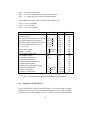
1
MARS CLIMATE DATABASE v4.3
USER MANUAL
(ESTEC Contract 11369/95/NL/JG
“Mars Climate Database and Physical Models”)
(CNES Contract “Base de donn´ees climatique martienne”)
F. Forget, E. Millour (LMD, Paris)
S. R. Lewis (The Open University, Milton Keynes)
April 2008
Abstract
This document is the User Manual for version 4.3 of the Mars Climate
Database (MCD) developed by LMD (Paris), AOPP (Oxford), Dept. Physics
& Astronomy (The Open University) and IAA (Granada) with the support
of the European Space Agency and the Centre National d’Etudes Spatiales.
This is a database of atmospheric statistics compiled from General Circulation Model (GCM) numerical simulations of the Martian atmosphere. This
document replaces previous documents which described versions 4.x, 3, 2,
and 1. and includes a thorough description of the access software provided
to extract and postprocess data from the database.
The database extends up to about 250 km in altitude; in addition to statistics on temperature, wind, pressure, radiative fluxes, it provides data such as
atmospheric composition (including dust, water vapor and ice content) and
make use of improved “dust and Extreme UltraViolet (EUV) scenarios” to
represent the variation of dust in the atmosphere and solar EUV conditions.
Linear interpolation in time of datafiles data is used to reconstruct variables
at user-specified time of day and solar longitude and various kind of vertical
coordinates may be specified as input. The data sets of version 4.3 are similar
to those of the previous version (exept for the files which contain information for large scale perturbation reconstruction, which have been updated).
As of version 4.2, the major improvement is in the MCD access software,
1
the Fortran routine “call mcd” which now include a “high resolution mode”
via postprocessing of MCD data which combines high resolution MOLA
(32 pixels/degree) topography and atmospheric mass correction from Viking
Lander 1 pressure records. Examples of interfaces for users interested in
calling subroutine “call mcd” from C or C++ programs or IDL, Matlab and
Scilab softwares are also given.
Two seperate light tools, “pres0”, which yields high resolution surface
pressure and “heights”, which converts various vertical coordinates are also
provided.
For descriptions of the contents and structure of the datafiles, details on
the dust distribution scenarios, a description of the variability models, and
of the high resolution postprocessing, see the Detailed Design Document.
Comparisons of MCD outputs with available measurements are addressed in
the Validation Document.
2
Contents
1
Introduction
5
1.1
Available Data. . . . . . . . . . . . . . . . . . . . . . . . . . . .
5
1.2
Database scenarios. . . . . . . . . . . . . . . . . . . . . . . . . .
6
1.3
High resolution mode . . . . . . . . . . . . . . . . . . . . . . . .
7
2
Differences Between Version 4.3 and Previous Versions of the MCD
7
3
Contents of the Mars Climate database
10
4
Installation
11
4.1
Software Requirements . . . . . . . . . . . . . . . . . . . . . . .
11
4.2
Installing the MCD from the DVD-rom . . . . . . . . . . . . . .
12
5
Ways to access the database
13
6
Using the CALL MCD subroutine
15
6.1
What is the CALL MCD subroutine ? . . . . . . . . . . . . . . .
15
6.2
Software Package . . . . . . . . . . . . . . . . . . . . . . . . . .
17
6.3
Compiling and running CALL MCD . . . . . . . . . . . . . . . .
18
6.4
CALL MCD input and output arguments
. . . . . . . . . . . . .
19
6.5
The right use of the CALL MCD subroutine . . . . . . . . . . . .
31
6.5.1
31
Perturbed atmospheres . . . . . . . . . . . . . . . . . . .
3
6.5.2
Running time . . . . . . . . . . . . . . . . . . . . . . . .
32
7
Calling the CALL MCD subroutine from IDL
34
8
Calling the CALL MCD subroutine from Matlab
37
9
Calling the CALL MCD subroutine from Scilab
37
10 Calling the CALL MCD subroutine from C or C++ programs
38
11 High accuracy surface pressure tool pres0
39
11.1 How to use pres0 . . . . . . . . . . . . . . . . . . . . . . . . .
39
11.2 Input/output of subroutine pres0 . . . . . . . . . . . . . . . . .
39
12 The heights tool
40
12.1 Arguments of heights subroutine . . . . . . . . . . . . . . . .
A Accessing the database without using the CALL MCD subroutine
41
42
A.1 Content of the database files . . . . . . . . . . . . . . . . . . . .
42
A.2 Using the NetCDF Library . . . . . . . . . . . . . . . . . . . . .
43
A.2.1 Opening and Closing Files . . . . . . . . . . . . . . . . .
45
A.2.2 Manipulating Data . . . . . . . . . . . . . . . . . . . . .
46
4
1
Introduction
The Mars Climate Database (MCD) is a database of atmospheric statistics compiled from state-of-the art General Circulation Model (GCM) simulations of the
Martian atmosphere (Forget et al., 1999). The models used to compile the statistics have been extensively validated using available observational data and represent the current best knowledge of the state of the Martian atmosphere given the
observations and the physical laws which govern the atmospheric circulation and
surface conditions on the planet.
Minor enhancements and additions may be performed after the delivery of this
version of the database. Such changes are given in the README file available on
line at http://www.lmd.jussieu.fr/˜forget/dvd/
where the up-to-date contents of DVD is always available.
The MCD can also be accessed in a variety of data formats using our interactive
Live Access Sever from our WWW site at
http://www-mars.lmd.jussieu.fr
1.1 Available Data.
The MCD contains several statistics on simulated data stored on a 5.625◦ × 3.75◦
longitude–latitude grid from the surface up to an approximate altitude of 300 km:
temperature, wind, density, pressure, radiative fluxes, atmosphere composition and
gases concentration, CO2 ice surface layer, turbulent kinetic energy, etc...
Fields are averaged and stored 12 times a day, for 12 Martian “months” to give
a comprehensive representation of the annual and diurnal cycles. Each month
covers 30◦ in solar longitude (Ls ), and is typically 50-70 days long. In other words,
at every grid-point, the database contains 12 “typical” days, one for each month. In
addition, information on the variability of the data within one month and the day
to day oscillations are also stored in the database. Software tools are provided to
reconstruct and synthetize this variability (section 6.1).
5
1.2 Database scenarios.
Eight combinations of dust and solar scenarios have been used because these are
the two forcings that are highly variable from year to year.
• On the one hand, the solar conditions describe variations in the Extreme UV
input which control the heating of the atmosphere above 120 km, which
typically varies on a 11 years cycle. Depending on the scenarios, solar maximum average and/or minimum conditions are provided.
• On the other hand, the major factor which governs the variability in the Martian atmosphere is the amount and distribution of suspended dust. Because of
this variability, and since even for a given year the details of the dust distribution and optical properties can be uncertain, multi-annual model integrations
were carried out for the database assuming various “dust scenarios”, i.e. prescribing various amount of airborne dust in the simulated atmosphere. 4 dust
scenarios are proposed :
1. The “Mars Year 24” (MY24) scenario was designed to mimic Mars as
observed by Mars Global Surveyor from 1999 to june 2001 1 , a martian
year thought to be representative of one without a global dust storm.
The dust fields were derived from MGS TES observations using data
assimilation technique. The MY24 scenario is provided with 3 solar
EUV conditions: solar min, solar ave, solar max.
2. The cold scenario corresponds to an extremely clear atmosphere (“Low
dust scenario”; dust opacity τ = 0.1), topped with a solar minimum
thermosphere.
3. The warm scenario corresponds to ”dusty atmosphere for the season”
scenario (but not a global dust storm), topped with a solar maximum
thermosphere.
4. The dust storm scenario represents Mars during a global dust storm
(dust opacity set to τ = 4). Only available when such storms are likely
to happen, during northern fall and winter (Ls=180-360), but with 3
solar EUV conditions: solar min, solar ave, solar max.
1
This corresponds to the 24th martian year according to the calendar proposed by R. Todd Clancy
(Clancy et al., Journal of Geophys. Res 105, p 9553, 2000) which starts on April 11, 1955 (Ls=0◦ ).
6
The “cold” and “warm” annual scenarios are provided to bracket the possible
global conditions on Mars outside global dust storms which are thought to
be highly variable locally and from year to year.
1.3 High resolution mode
The Mars Climate Database has been compiled from the output of a general circulation model in which the topography is very smoothed because of its low resolution.
In addition, the pressure variations due to the CO2 cycle (condensation of atmospheric CO2 in the polar caps) that is computed by the model is only based on the
simulation of the actual physical processes. The polar cap physical properties have
been tuned to somewhat reproduce the observations, but no correction was added.
As of version 4.2, access software includes a “high resolution” mode which
combines high resolution (32 pixels/degree) MOLA topography and the smoothed
Viking Lander 1 pressure records (used as a reference to correct the atmospheric
mass) with the MCD surface pressure in order to compute surface pressure as accurately as possible. The latter is then used to reconstruct vertical pressure levels
and hence, within the restrictions of the procedure, yield high resolution values of
atmospheric variables.
The procedure by which high accuracy surface pressure is computed is also
implemented as a light and autonomous tool, pres0 (see section 11).
2
Differences Between Version 4.3 and Previous Versions
of the MCD
Differences between version 4.3 and version 4.2
• The main upgrade in MCD version 4.3 is the improvement of the large scale
perturbation model. Version 4.3 thus uses the same database datafiles as
version 4.2, except for a subset which contains updated data required for the
large scale perturbation model.
• Other changes that have been introduced are:
7
– An additional vertical coordinate (‘zkey’ parameter) may be used to
specify vertical coordinate as altitude above reference radius (arbitrarily set to 3.396106 m).
– The output unit to which messages are written is now a parameter that
can be set by the user (the default output unit is set to 6, which implies,
in conformance with Fortran standards, the standard output).
– In order for the whole MCD to fit in a single DVD, some datafiles (all
those which contain data about dust storm sceanarios, i.e. files in the
data directory with names starting with strm) have been compressed
(gzipped) and should be un-compressed (gunzipped) before being used.
Differences between version 4.2 and version 4.1
• Version 4.2 uses the same database datafiles as version 4.1, except for a small
subset (the files which contain variability); most improvements, changes and
new features are in the access and postprocessing software.
• The main new features and differences are:
1. The main Fortran subroutine to retrieve data from the database is now
called “call mcd” and significant changes to the argument list, compared to its predecessor “atmemcd”, have been introduced:
– A new high resolution procedure (based on the integration of high
resolution 32 pixels per degree MOLA topography) has been implemented.
– Input and output arguments which are floating numbers are now
declared as single precision (i.e. Fortran REAL), except ’xdate’,
which is double precision, (i.e. Fortran REAL*8).
– The way by which users impose date and local time has changed.
– Input longitude and latitude must now be given in degrees.
Longitude is interpreted as degrees east (as before).
– Input arguments used to signal and generate perturbations have
been changed.
– Day to day variability of atmospheric variables is now given either
pressure-wise or altitude-wise, depending on the vertical coordinate selected by the user.
2. Examples of interface software for C, C++ and Scilab users, have been
added (in addition to the pre-existing IDL and Matlab ones).
8
3. Computation of solar longitude (from a given Julian date) has been
made more accurate. Computation of local time (given in true solar
time) has been improved by using an appropriate equation of time.
4. The “pres0” tool has been updated.
Lists of changes and improvements of previous versions of the MCD
• Version 4.1 is similar to beta version 4.0 with some improvements and a few
problems fixed.
• The main differences between version 4 and previous version 3.1 are:
1. The database now extends up to the thermosphere and new variables
(upper atmospheric composition: CO2 , N2 , CO, O, H2 and, in the lower
atmosphere: water, water ice, ozone, dust) are available.
2. Different vertical coordinates may be specified as input, including pressure level.
3. A linear interpolation in time (Ls) for mean variables between seasons
was added.
4. For some variables, an estimation of the “day to day” variation is provided (root mean square values).
5. There is a significant re-arrangement of arguments of atmemcd so that
all the input variables are followed by all the output variables.
6. We suggest the use of direct compilation rather than using the UNIX
command “make”.
7. Variables are now saved in atmemcd to fix problems with F77 compilers which don’t store values of variables between subroutine calls.
8. The database now has a more accurate representation of gravity; the
fact that it varies following an inverse square law is accounted for when
integrating the hydrostatic equation. The variation of R, the gas constant, with altitude is also taken into account.
9. The horizontal resolution of the database has changed to 5.625◦ ×3.75◦
(longitude × latitude).
10. We now provide the separate tool to compute surface pressure with
high accuracy.
11. We now provide some tool to use the database software from IDL.
9
• A major change in Version 3.1, compared to version 3.0 of the database, is
the change from DRS data format to NetCDF. A bug was also fixed for the
calculation of large scale variability in the upper atmosphere (above 120
km).
• The main differences between version 3.0 and 2.3 are mostly related to the
content of the database files, due in particular to improvements made in the
models used to build the database, including an extension of the model top
from 80 to 120 km, improved surface properties and a dust scenarios from
Mars Global Surveyor.
• The main difference between version 2.3 and 2.0 is the use of the main
subroutine ATMEMCD which computes meteorological variables from the
Mars Climate Database (MCD).
• The main difference between version 2.0 and 1.0 of the MCD is that the
large-scale variability model now makes use of two-dimensional, multivariate Empirical Orthogonal Functions (EOFs). These now describe correlations in the model variability as a function of both height and longitude
(rather than solely of height as in version 1.0).
3
Contents of the Mars Climate database
The contents of each subdirectory of the MCD provided on the DVD are summarized here.
docs This directory contains files in pdf formats which can be used to print further
copies of the documentation:
– The User Manual (user manual.pdf) of the database; this document.
– pdf versions of the scientific reference articles Lewis et al. (1999) and
Forget et al. (1999) describing earlier Mars Climate database and the
General Circulation models used to compile it are also provided.
mcd This directory contains Fortran source code for the climate database access softwares (see section 6, and the README file in the directory): the
CALL MCD subroutine, and a test program.
10
Subdirectory testcase contains a simple tool to test the results from the
software after installation.
Subdirectory pres0 contains an autonomous tool to compute surface pressure in the context of high resolution topography (see section 4.2).
Subdirectories idl, matlab, scilab and c interface contain examples of interfaces of the Fortran subroutine with other languages and softwares.
data The full MCD datasets derived from model runs. The database is contained
in one DVD-ROM. You can (should) copy the entire database on your hard
disk (and also decompress some of the data files, see section 4.2).
4
Installation
4.1 Software Requirements
• The MCD is primarily designed to operate in the Unix/Linux environment
on a PC or a workstation . Access software is written in Fortran77, for
which a Fortran compiler (77, 90, 95 etc...) is needed.
Because the NetCDF libraries (see below) are also available under Windows
systems, several users have succefully compiled and used the access software
as under Unix/Linux. Nevertheless, it has not been fully tested by the our
team but we can confirm that it compiles fine under the Cygwin environment
on Windows using the GNU g77 compiler.
• The data in the MCD are written using the Network Common Data Form
(NetCDF) software. It was developed as part of Unidata , a National Science
Foundation-sponsored program (see Detailed Design Document for more details). The libraries are freely available from the Unidata web site :
http://www.unidata.ucar.edu/software/netcdf/
NetCDF works on most current operating systems, including:
– AIX
– HPUX
– IRIX
– Linux
– MacOS X
– OSF1
– SunOS-4, Solaris (Sparc and i386)
– MS Windows
11
4.2 Installing the MCD from the DVD-rom
1. Create a working directory, e.g. mars, on a disk where you wish to use the
database.
2. Copy the following directory from the DVD-rom to this location: at least
mcd, and if needed docs.
3. If possible, you should copy the data from the DVD-ROM to your hard disk.
The data can be accessed directly from the DVD-ROM (see below), but this
last solution is slower and less convenient. We suggest that you copy the
directory data from the DVD-ROM to the working directory mars for instance, or to another disk if there is not enough disk space available there
(see how to link datafiles and software below). Moreover, as of MCD version
4.3, storage requirements have imposed that some of the data files be compressed (gzipped) and should be uncompressed (gunzipped; i.e. gunzip
file.gz on Unix machines; any of the many standard (de-)compression
tool will do on other platforms) prior to being used. Only files containing
data for dust storm scenarios (i.e. files in the data directory whith a name
starting with strm) have been compressed. This way the MCD can still
be run with all the data remaining on the DVD (the dust scenario obviously
cannot be used then). A full installation of the MCD takes about 4.5 Gb of
disk space. Note that the amount of disk space needed may be reduced by
only retaining a limited range of dust scenarios or seasons of interest within
the data subdirectory (see Appendix A for a quick description of database
file contents).
4. In the working directory (e.g. mars) it is convenient to set up a MCD DATA
symbolic link2 in the same directory to point to the data directory, wherever
it has been stored:
ln -s /full/path/to/mcd/data MCD DATA
For instance, if one wishes to access the data directly from the DVD-ROM,
If the DVD-ROM is mounted as /dev/dvdrom then create the link :
ln -s /dev/dvdrom/data MCD DATA
N.B In the call mcd subroutine , the path to the directory can be given as
an input using the dset argument (e.g. dset=’/dev/cdrom/data/’)
2
This ”symbolic link” strategy unfortunately does not work with Windows where the full path to
the data directory must be used.
12
although by default the subroutine will use MCD DATA/ if dset is not initialized or set to ’ ’.
5. If NetCDF is not available on your system, you must install the NetCDF
library following the instructions given on their www site (see above). For
this purpose, you have the choice either to build and install the NetCDF
package from source, or use prebuilt binary releases if they are available for
your platform (check the ”Frequently Asked Question”).
Ideally, you can install the full NetCDF package as recommanded on the
web site. In practice, the minimum you need to run the access software are
only two files : an include file named netcdf.inc and a Fortran library
file named libnetcdf.a. The version of the files depends of the machine
and of the compiler. An easy way to get them is to go to the unidata netcdf
web page, click on precompiled binaries, download a compressed file corresponding to your operating system, uncompress the file. You’ll find the
netcdf.inc in the include directory, and the libnetcdf.a in the
lib directory. You’ll need to provide the path to these two files when compiling applications (see the compile files in the database). Unfortunately,
this does not always work : if your compiler doesn’t work with the precompiled library, you will have to recompile Netcdf with it, and follow the web
site instructions.
5
Ways to access the database
There are three main ways of accessing data from the MCD which have been implemented to date.
Firstly, if you know Fortran, the best way to retrieve environmental data from
the Mars climate database at any given locations and times is to use the subroutine
mode of the software supplied with the Mars Climate Database. In practice, one
only has to call a main subroutine named call mcd from within any program
written in Fortran. A simple example of such a program (test mcd.F), which
can be easily modified, is provided. This mode was developed with particular
attention to trajectory simulation applications, but it can also be used for most
other purposes. Further information on the use of call mcd are available below.
13
Secondly, users who prefer using IDL, Matlab or Scilab software, or who
program in C and/or C++ will find examples of how to interface their favorite
tools with the Fortran subroutine call mcd in corresponding subdirectories (see
sections 7 to 10).
Thirdly, it is possible to access the database directly from within any program
written in any high level language or software which can read NetCDF files. This
gives the most flexibility for particular applications (e.g. when one wants to handle
global fields), although it does demand a greater understanding of how the database
contents are organised (see appendix A), as well as of how the variability models, if
these are required, should be used. The Fortran subroutines used by the call mcd
routine (included in file call mcd.F) illustrate how to open and read the database
files.
If you are interested in inspecting/plotting mean and standard deviation data
from the raw database datafiles, you can install the Grid Analysis and Display
System (GrADS) or Ferret which are fine free softwares for displaying graphical
output from geophysical datasets. GrADS and Ferret can read NetCDF files and
display their contents using a few easy instructions. Both works on Unix/Linux
and Windows environments, and can be downloaded from their respective World
Wide Web servers:
http://grads.iges.org/grads
http://ferret.pmel.noaa.gov/Ferret
There are also freely available plotting tools such as ncview or ncBrowse which
can be used to visualize NetCDF files. IDL users can also read and display the raw
datafiles using the “read ncdf.pro” IDL function available on many websites.
Please note that the vertical coordinate in the datafiles are terrain-following
“sigma-pressure” hybrid coordinates. The “altitude” coordinate given in the datafiles
is merely an approximation of the real altitude of the data. The Fortran access software calculates heights accurately by integrating the hydrostatic equation directly
on the hybrid coordinates.
14
6
Using the CALL MCD subroutine
6.1 What is the CALL MCD subroutine ?
The purpose of the call mcd subroutine is to extract and compute meteorological variables useful for atmospheric trajectory computations as well as scientific
studies. Data which may thus be obtained includes:
•
•
•
•
•
•
•
•
•
•
•
Atmospheric and surface pressure
Atmospheric and surface temperature
Density
Radiative fluxes (Solar and thermal IR) on the ground and at the top of the
atmosphere
Wind speed defined by two components the meridional wind (positive when
oriented from south to north) the zonal wind (positive when oriented from
west to east)
Vertical wind
The main atmospheric composition : CO2 , N2 , O, CO volume mixing ratio
Water vapour and water ice content
Dust aerosol content
Ozone (O3 ) content
Air viscosity, heat capacity and Cp /Cv ratio
The Fortran subroutine call mcd retrieves database data at any date (Earth
date or Mars season and time) and at any point in space defined by latitude and east
longitude and a vertical coordinate which can be a distance from the planet center,
an altitude, or a pressure level. The returned values of meteorological variables
are computed by interpolation in space, time of day and month from data stored in
the MCD. As of version 4.2 of the MCD an additional high resolution interpolation
procedure (which uses 32 pixels/degree MOLA topography) has been implemented
to simulate local pressure and density as accurately as possible.
Above the top level of the database density and pressure are estimated by integration of the hydrostatic equation assuming a constant temperature.
15
For these variables, the subroutine delivers mean values and, if requested, adds
a different type of perturbation to density, pressure, temperature and winds. The
available types of perturbation are :
• Small scale perturbations due to the upward propagation of gravity waves
for any altitudes (there is no small scale perturbation for surface pressure).
• Large scale perturbations due to the motion of baroclinic weather systems
and other transient waves. These perturbations are correlated in longitude
and altitude, and are reconstructed from the actual system predicted by the
model.
• Perturbations equal to n times the RMS day to day variation for all variables.
The two first types of perturbation have a random component. A comprehensive explanation of the perturbations is included in the Detailed Design Document3
3
In summary the perturbations are calculated as follow :
• The gravity wave perturbation of a meteorological variable is calculated by considering
vertical displacements of the form
δz = δh sin
2πz
+ φ0
λ
(1)
where λ is a characteristic vertical wavelength for the gravity wave and φ0 is a randomly
generated surface phase angle. surface angle. δz is the amplitude of the wave depending
on the height z. δh is the sub-grid scale surface roughness (the variability on scales smaller
than the explicit database resolution) and is a function of location on the Martian surface.
If z is higher than 100 km, the amplitude of the wave is taken to be equal to the amplitude
at 100 km.The amplitude of the wave is limited to λ/2/π to saturate the amplitude of the
perturbation when it becomes statically unstable.
• The large scale perturbation in the Mars Climate Database is represented using a technique
that is widely used in meteorological data analysis, namely, Empirical Orthogonal Function
(EOF) analysis. A two-dimensional, multivariate EOF of the main atmospheric variables
(surface pressure, atmospheric temperature and wind components) is used which describes
correlations in the model variability as a function of both height and longitude. 200 EOFs
have been retained in the series in order to reproduce the variability of the original fields.
Above the top level of the database, the perturbation represents a constant percentage of the
mean value this percentage is equal to those at the top of the database.
• For the last type of perturbation (i.e. n times the standard deviation), the standard deviation
is interpolated from the day to day RMS variabilities stored in the database. If the user works
with pressure as the vertical coordinate, then the added variabilities are pressure-wise, and
altitude-wise otherwise. Above the top level of the database, the standard deviation represents
a constant percentage of the mean value ; this percentage is equal to those at the top of the
database.
16
6.2 Software Package
The call mcd subroutine is in directory mcd. This directory includes:
• README, a short text file which summarizes the information contained here.
• File call mcd.F, which contains the CALL MCD main subroutine and
most of the subroutines and functions it calls.
• the include file constants mcd.inc used by call mcd and subsidiary
routines.
• File test mcd.F which contains a simple and straightforward illustration
of a program using call mcd and julian.
• The compile file which contains an example of the (Unix) command line
to compile the subroutine and program.
• The file test mcd.def contains a list of input data for test mcd (see
section 6.3).
• A subdirectory testcase containing test cases used to test the accuracy of
your installation of the database
• the julian.F file, which contains a subroutine which computes the Julian
date corresponding to a given calendar date.
• the heights.F file which contains the subroutines necessary to convert
distances expressed as distance to planet center, height above areoid and
height above local surface. Given any of these, this routine computes the
other two, either at GCM grid resolution or using high (1/32 degree) resolution (see section 12). call mcd does these conversions using these routines
so users need not use it. These routines are nonetheless kept seperate from
the main file call mcd.F for specialists who might want to use it seperately.
• subdirectory pres0 which contains the pres0 tool (see section 11).
• subdirectories idl, matlab, scilab and c interfaces which contain
examples of interfaces.
17
6.3 Compiling and running CALL MCD
A simple program using the call mcd subroutine (as well as the complementary
subroutine julian) called test mcd is provided in the mcd directory. You can
easily modify it or use part of this code for your own purpose. To compile the
program, edit the compile file and make the necessary changes (ie: compiler
name, path to NetCDF library and include file). Then, For instance, to compile and
run test mcd, type4 :
> compile
> test mcd
Then, just answer the questions...
Alternatively you can edit the file test mcd.def and redirect it to test mcd:
> test mcd < test mcd.def
In the mcd/testcase sub-directory, a tool to test that call mcd is running accurately on your computer (using test mcd) is provided. Please read
mcd/testcase/README for further information.
If your machine runs under Windows you have 2 solutions:
1. Install a Unix environment emulator for Windows. The most popular is Cygwin, which you can download from http://www.cygwin.com. This
emulator includes most Unix features and softwares. NetCDF libraries can
be built on Cygwin as easely as on other Unix systems. As far as a few tests
have shown, requirements and steps necessary to install the Mars Climate
Database and use the provided access software under Cygwin are in fact the
same as those for ’standard’ Unix systems.
2. Port the Mars Climate Database to Windows. We have not fully tested
that possibility, but several users have done so successfully. NetCDF librairies for Windows can be dowloaded from the NetCDF official website at:
http://www.unidata.ucar.edu/packages/netcdf Note that, with
Windows, the ”symbolic link strategy” to the Mars Climate Database data
4
In the examples given here, the > at the begining of command lines is the Unix session command
prompt.
18
directory described in section 4.2 will not work; the ’true’ path to that directory must be used in the Fortran routines and programs (see variable dset
in the description of call mcd arguments in section 6.4).
6.4 CALL MCD input and output arguments
A Fortran call to subroutine call mcd should look something like:
call_mcd(zkey,xz,xlon,xlat,hireskey,
&
datekey,xdate,localtime,dset,scena,
&
perturkey,seedin,gwlength,extvarkey,
&
pres,dens,temp,zonwind,merwind,
&
meanvar,extvar,seedout,ier)
All the input arguments (ie: values which must be set before calling the routine
and which are not altered by it) are described in table 1. Outputs are described in
table 2.
As call mcd runs, it writes informational (and error) messages to standard
output. Users who wish to run call mcd silently (i.e. without any messages sent
to standard output) should edit file constants mcd.inc and change the value
of parameter output messages to .false.
As of version 4.3 the ”standard output” unit number which will be used by call mcd
is set to the value of the out parameter, also defined in file constants mcd.inc.
The default value of out is 6, which is the standard value preconnected to the
screen (on most systems). Setting out to any other positive integer value n (except 5 which is the usually preconnected to standard input) will send messages to
the corresponding file. It is thus advised to open the corresponding file (using Fortran command open(unit=n,file="myfilename")) prior to any call to
call mcd otherwise default file fort.n will be used (this behaviour is possibly
system-dependent).
19
Table 1: CALL MCD Input arguments
Name
zkey
Type
integer
Description
Flag to set the type of vertical coordinate xz is given as:
1: xz is the radial distance from the center of the planet (m).
2: xz is the altitude above the Martian zero datum (Mars
geoid or “areoid”), in meters.
3: xz is the altitude above the local surface (m).
4: xz is the pressure level (Pa).
5: xz is the altitude above reference radius (3.396 106 m)
(m).
N.B. The zero elevation is defined as the gravitational equipotential surface whose average value at the equator is equal to the
mean radius as determined by MOLA. For more informations, see
http://ltpwww.gsfc.nasa.gov/tharsis/mola.html.
Depending on the value of flag hireskey, references to areoid and topography are with respect to GCM grid or high resolution MOLA data.
xz
real
xlon
xlat
hireskey
real
real
integer
Vertical coordinate of the requested point. Its exact definition
depends on the value of input argument zkey.
East Longitude (planetocentric), in degrees.
Latitude (planetocentric), in degrees.
Flag to set the resolution at which data retrieval and postprocessing should be done:
0: Interpolate data from GCM grid.
1: Use high resolution (32 pix/deg.) MOLA topography and
areoid, as well as some internal post-processing scheme
to reconstruct data (see section 1.3).
20
Table 1: CALL MCD Input arguments (continued)
datekey
integer
Flag to set the way dates (xdate and localtime) should be
interpreted:
0: “Earth time”; xdate is given in Julian days. With
datekey=0, the localtime argument, although unused, must be set to zero.
1: “Mars time”; xdate is the value of the solar longitude Ls
and localtime is the local true solar time at longitude
lon, given in martian hours.
xdate
double
precision
(REAL*8)
• if datekey=0: the Julian date.
• if datekey=1: the solar longitude Ls (in degrees), Ls ∈
[0 : 360]
N.B. The subroutine julian.F can be used to compute the Julian date corresponding to a given calendar date (day, month, year, hours, minutes, seconds)
on Earth.
localtime
real
Local true solar time at longitude lon, in martian hours. Should
only be specified if datekey=1 and must be set to zero if
datekey=0.
N.B. Local true solar time is such that the sun is highest in the sky at noon. A
martian hour is defined as 1/24th of a sol (a martian day, which is 88775.245
s long).
dset
character
string
dim(*)
Path to the directory where the datafiles are to be found.
dset may be of any size. If dset is an empty string, then the
path to the datasets is set the default path MCD DATA/.
N.B. the given path must end with a “/” (e.g.: /home/data/) on Linux and
“\” on Windows.
21
Table 1: CALL MCD Input arguments (continued)
scena
integer
Dust and solar EUV input scenario :
1 = MY24 dust Scenario, solar minimum conditions
2 = MY24 dust Scenario, solar averaged conditions
3 = MY24 dust Scenario, solar maximuml conditions
4 = dust storm τ = 4, solar minimum conditions
5 = dust storm τ = 4, solar averaged conditions
6 = dust storm τ = 4, solar maximum conditions
7 = warm scenario: Viking lander dust, solar max
8 = cold scenario: low dust , solar min.
N.B. The solar conditions describe variations in the Extreme UV input which
control the heating of the atmosphere above ∼120 km, which typically varies
on a 11 years cycle. The different dust scenarios differ by dust amount and
distribution used to create the data files (dust is highly variable on Mars from
year to year).
The “Mars Year 24” (MY24) scenario was designed to mimic Mars as observed by Mars Global Surveyor in from 1999 to june 2001, a martian
year though to be typical.
The warm and cold scenario are provided to bracket the possible dust content of the atmosphere, outside global dust storms.
dust storm τ = 4 represents Mars during a global dust storm (dust opacity
set to 4). Only available when such storms are likely to happen, during
northern fall and winter (Ls=180-360).
Please see the Detailed Design Document for further information.
perturkey
integer
Flag to set the type of perturbation to add.
1: None.
2: Add large scale perturbations (using EOFs).
3: Add small scale perturbations (gravity waves).
4: Add small and large scale perturbations.
5: Add seedin times the standard deviation.
N.B. For the small scale or large scale perturbations, a seed for the random
number generator must be specified (see seedin argument). When large
scale perturbation is requested, as long as seedin remains the same, no new
random vector is generated and you work with the same correlated perturbed
atmosphere.
22
Table 1: CALL MCD Input arguments (continued)
seedin
real
• if perturkey=1, 2, 3 or 4: Random number generator
seed and flag.
For the first call to call mcd, this value (in fact its integer part) is used to seed the random number generator.
If the value of seedin is changed between subsequent
calls to call mcd, it triggers the reseeding of the random number generator and subsequently the regeneration
of a new perturbed atmosphere (see section 6.5.1).
• if perturkey=5: coefficient by which the standard deviation should be multiplied before being added to the
mean value. seedin is then not allowed to be more than
4 or less than −4.
gwlength
real
Wavelength of the vertical gravity wave (in meters).
Used for small scale perturbations (ie: if perturkey=3 or 4).
Should be between 2000 and 30000 m; if set to 0 then a default
value of 16000 m is used.
N.B. Feature for specialists: Changing the value of gwlength between calls
to call mcd triggers the generation of a new random phase for the gravity
wave (and without altering the large scale perturbation, if the later is also
requested, i.e. in the perturkey=4 case).
extvarkey
integer
Flag to request extra variables on output
0 = extra variables not computed (only the 7 first elements of
output array extvar will be filled). Faster computations
1 = extra variables computed and returned in output argument
array extvar
23
Table 2: CALL MCD output arguments
Name
pres
dens
temp
zonwind
merwind
meanvar
Type
real
real
real
real
real
real
(dim 5)
description
Atmospheric pressure (Pa)
Atmospheric density (kg/m3 )
Atmospheric temperature (K)
Zonal component of wind, in m/s (> 0 if eastward)
Meridional component of wind, in m/s (> 0 if northward)
“mean” atmospheric values
• meanvar(1) = mean atmospheric pressure
• meanvar(2) = mean atmospheric density
• meanvar(3) = mean atmospheric temperature
• meanvar(4) = mean zonal wind
• meanvar(5) = mean meridional wind
This array contains the unperturbed values of pres, dens,
temp, zonwind and merwind (i.e.: In the perturkey=1
case, where no perturbation are requested, the meanvar array
will contain these).
N.B. Close to the surface (i.e. below the lowest MCD level, which is around
4.5 m above the ground, and down to the aerodynamic roughness length of
1 cm) the horizontal winds fall logarithmically to zero, following classical
boundary layer theory. If you want near-surface winds, then sample at a range
of non-zero heights close to the surface as appropriate for your application.
24
Table 2: CALL MCD output arguments (continued)
extvar
real
(dim 100)
Supplementary variables array
(extvar(1) to extvar(7) provides time and space coordinate which
are always computed and are therefore always set. extvar(8)
to extvar(50) are only computed and set if input argument
extvarkey=1. These are otherwise set to zero. The rest of
the array, extvar(51) to extvar(100) is unused (yet) and always
set to zero.
These supplementary variables are usually not used for atmospheric trajectory computations but are useful for environmental
studies:
• extvar(1)= Radial distance to planet center (m).
• extvar(2)= Altitude above areoid (Mars geoid) (m).
• extvar(3)= Altitude above local surface (m).
• extvar(4)= Orographic height (m) (altitude of the surface
with respect to the areoid).
N.B. Depending on the value of input flag hireskey, references to
altitudes and orographic height are with respect to GCM grid or high
resolution MOLA topography and areoid.
• extvar(5)= Ls, solar longitude of Mars (deg).
• extvar(6)= LTST Local True Solar Time at longitude lon
(in martian hours = 1/24 of a mars day).
• extvar(7)= Universal solar time (LTST at lon=0) (hrs).
• extvar(8)= Cp: Air specific heat capacity (J.kg−1 .K−1 ).
• extvar(9)= γ = Cp/Cv Ratio of specific heats.
• extvar(10)= RMS day to day variations of density
(kg/m3 ).
N.B. The given RMS is either pressure-wise (if zkey=4) or altitudewise (if zkey=1, 2 or 3).
25
Table 2: CALL MCD output arguments (continued)
•
•
•
•
extvar(11)= Not used (set to zero).
extvar(12)= Not used (set to zero).
extvar(13)= Scale height H(p) (m).
extvar(14)= GCM orography (m) (will be equal to
extvar(4) if input parameter hireskey=0).
N.B. Provided for specialist interested in the differences between low
resolution (i.e.: the GCM resolution) and high resolution MOLA topography.
• extvar(15)= Surface temperature (K).
• extvar(16)= Daily maximum mean surface temperature
(K).
• extvar(17)= Daily minimum mean surface temperature
(K).
• extvar(18)= Surface temperature RMS day to day variations (K).
• extvar(19)= Surface pressure (Pa) (high resolution if
hireskey=1, GCM surface pressure if hireskey=0).
• extvar(20)= GCM surface pressure (Pa) (will be equal to
extvar(19) if hireskey=0).
N.B. Provided for specialist interested in the differences between low
resolution (i.e.: the GCM resolution) and high resolution surface pressures.
26
Table 2: CALL MCD output arguments (continued)
• extvar(21)= Atmospheric pressure RMS day to day variation (Pa), if zkey=1, 2 or 3. Otherwise set to zero.
• extvar(22)= Surface pressure RMS day to day variations
(Pa).
• extvar(23)= Atmospheric temperature RMS day to day
variations (K).
N.B. The given RMS is either pressure-wise (if zkey=4) or altitudewise (if zkey=1, 2 or 3).
• extvar(24)= Zonal wind RMS day to day variations (m/s).
N.B. The given RMS is either pressure-wise (if zkey=4) or altitudewise (if zkey=1, 2 or 3).
• extvar(25)= Meridional wind RMS day to day variations
(m/s).
N.B. The given RMS is either pressure-wise (if zkey=4) or altitudewise (if zkey=1, 2 or 3).
• extvar(26)= Vertical wind (m/s) (positive when downward).
• extvar(27)= Vertical wind RMS day to day variations
(m/s).
N.B. The given RMS is either pressure-wise (if zkey=4) or altitudewise (if zkey=1, 2 or 3).
• extvar(28)= Small scale density perturbation (gravity
wave) (kg/m3 ).
• extvar(29)= q2: turbulent kinetic energy (m 2 /s2 ).
• extvar(30)= Not used (set to zero).
27
Table 2: CALL MCD output arguments (continued)
• extvar(31)= Thermal IR (λ > 5µm) flux to surface
(W/m2 ).
• extvar(32)= Solar flux (λ < 5 µm) to surface (W/m2 ).
• extvar(33)= Thermal IR flux to space (W/m2 ).
• extvar(34)= Solar flux reflected to space (W/m 2 ).
• extvar(35)= Surface CO2 ice layer (kg/m2 ).
• extvar(36)= DOD: Dust column visible optical depth.
N.B. DOD is in fact deduced from the dust opacity retrieved by M.
Smith (GFDL) from MGS TES at 1075 cm−1 , multiplied by 1.65. To
estimate a true visible extinction optical depth, we suggest to multiply
DOD by about 1.2.
• extvar(37)= Dust mass mixing ratio (kg/kgair ).
• extvar(38)= Dust Optical Depth RMS day to day variations.
• extvar(39)= Not used (set to zero).
• extvar(40)= Water vapor column (kg/m 2 ).
N.B. If you prefer to have this value in precipitable microns (pr-µm;
i.e. g/m2 ), then simply multiply it by 1000.
28
Table 2: CALL MCD output arguments (continued)
•
•
•
•
•
•
•
•
•
•
extvar(41)= Water vapor vol. mixing ratio (mol/mol).
extvar(42)= Water ice column (kg/m2).
extvar(43)= Water ice mixing ratio (mol/mol).
extvar(44)= O3 (ozone) volume mixing ratio (mol/mol)
(set to 0 above the 4.10−4 Pa level, which is around 120 km).
extvar(45)= [CO2] volume mixing ratio (mol/mol) (set to
9.532 10−1 when below the thermosphere which starts at ∼90 km).
extvar(46)= [O] volume mixing ratio (mol/mol).
extvar(47)= [N2] volume mixing ratio (mol/mol) (set to
0.027 when below the thermosphere).
extvar(48)= [CO] volume mixing ratio (mol/mol) (set to
8 10−4 when below the thermosphere).
extvar(49)= R : Molecular gas constant (J.kg−1 .K−1 ).
extvar(50)= Air viscosity v estimation (N s m−2 ).
N.B. v = AT 0.69 /0.25(4Cp + 5R), with A = ΣAi vmri , where
vmri is the vol. mixing ratio of specy i, and ACO2 = 3.07 10−4 ,
AO = 7.6 10−4 , AN2 = 5.5 10−4 , ACO = 4.87 10−4 and AAr =
3.4 10−4 .
• extvar(51) to extvar(100): Not used (set to zero).
seedout
real
The current index of the random number generator.
May be used to trigger (by setting seedin to this value) the
generation of a new set of perturbations for the next call to
call mcd.
29
Table 2: CALL MCD output arguments (continued)
ier
integer
Status code: When an error occurs in call mcd, all the outputs arguments (pres, dens, temp, zonwind, merwind,
all elements of meanvar and extvar)are set to −999 and a
message is written to the standard output. The value of ier
summarises the status of call mcd :
0: OK (no error)
1: Wrong vertical coordinate flag zkey
2: Wrong choice of dust scenarion scena
3: Wrong value for perturbation flag perturkey
4: Wrong value for high resolution flag hireskey
5: Wrong value for date flag datekey
6: Wrong value for extra variables output flag extvarkey
7: Wrong value for latitude xlat
8: Inadequate value for gravity wave wavelength
gwlength
9: Wrong value of input solar longitude (xdate must be in
[0:360], in the datekey=1 case)
10: Given Julian date xdate (in the datekey=0 case) implies an Earth date outside of [1800:2200] range
30
Table 2: CALL MCD output arguments (continued)
11: Wrong value of local time (in the datekey=1 case),
which should be in [0:24]
12: Incompatible localtime6=0 and datekey=0
13: Unresonable value of seedin (in perturkey=5 case)
14: No dust storm scenario available at such date
15: Could not open a database file (dset is probably wrong)
16: Failed loading data from a database file
17: Sought altitude is underground
18: adding (perturkey=5) perturbation yields unphysical
density
19: adding (perturkey=5) perturbation yields unphysical
temperature
20: adding (perturkey=5) perturbation yields unphysical
pressure
21: Could not open a database file file but found that a corresponding gzipped file.gz version of the file exists.
You should got to the dset directory and de-compress it
(e.g. gunzip file.gz on Unix systems).
6.5 The right use of the CALL MCD subroutine
6.5.1
Perturbed atmospheres
The perturbation consisting of adding n times the standard deviation to the
mean value (the perturkey = 5 case) must not be used to create randomly
perturbed atmospheres, but only as a mean to globally overestimate or underestimate the profiles of the meteorological variables. To generate randomly perturbed
atmospheres you must use small or large scale perturbations which take into account some correlation of perturbations in the space and between variables. Then
31
when you use the perturkey = 5 perturbation, you have to keep the same
seedin (ie: multiplying factor) along the whole trajectory to avoid introducing
unrealistic gradients between consecutive values.
When generating a randomly perturbed atmosphere using the large scale perturbations (perturkey = 2 or 4) to simulate a trajectory, the value of seedin
should be kept constant in order to work with the same correlated perturbed atmosphere.
Reseting the large scale perturbations (by modifying the value of seedin between
calls to call mcd) to build profiles at a given location should only be done in the
context of generating a range of different possibilities (an example is given in table 3).
When using the perturbation due to gravity wave propagation (small scale
perturbation) (preturkey = 3 or 4), to generate a vertical profile, the phase
(ie: the value of seedin), as well as the associated wavelength gwlength should
remain fixed.
Note that if computing a group of trajectories clustered over a small horizontal distance (and at a given martian time), then perturbations should not be reset
between the computation of each trajectory in order to retain the underlying correlation of the perturbations.
Note for specialists: It has been made possible to keep a given large scale perturbation whilst only changing the gravity wave small scale perturbation between
calls. This is achieved by changing the value of input argument gwlength between calls to call mcd. This feature, which should be usefull to people who
might want to generate “realistic” longitude-height or latitude-height slices over
large horizontal distances (over which indeed gravity waves should not correlate),
requires some sensible choices in longitude/latitude spacing and gravity waves reseeding. It is meant for experienced users and not advised for general use.
6.5.2
Running time
In order to minimize computational time, the datasets corresponding to encompassing months (of sought input date) are read and loaded from the database at the first
call of the ’call mcd’ subroutine. This initial loading is time consuming, but once
loaded these values can then be used for further calls, as long as the sought dates
32
Table 3: Example of Fortran code to illustrate the use of (re-)setting perturbations
! build a density profile at a given time and location
! with EOF and GW perturbations
perturkey=4
seedin=100
! seed perturbations
zkey=3 ! work in "altitude above local surface" coordinate
do i=1,100
xz=(i-1)*2000.0 ! go from surface to 200km
call_mcd(zkey,xz,xlon,xlat,hireskey,
&
datekey,xdate,localtime,dset,scena,
&
perturkey,seedin,gwlength,extvarkey,
&
pres,dens,temp,zonwind,merwind,
&
meanvar,extvar,seedout,ier)
profile(1,i)=dens ! store density
enddo
!
! ... some code here...
! ... moved on to a different time or place ’far’ from previous one
! ... such that perturbations should be reset
!
seedin=seedout ! change seedin to regenerate perturbations
! build the new density profile
do i=1,100
xz=(i-1)*2000.0 ! go from surface to 200km
call_mcd(zkey,xz,xlon,xlat,hireskey,
&
datekey,xdate,localtime,dset,scena,
&
perturkey,seedin,gwlength,extvarkey,
&
pres,dens,temp,zonwind,merwind,
&
meanvar,extvar,seedout,ier)
profile(2,i)=dens ! store density
enddo
33
Table 4: Illustrative example of the impact of call mcd options on its run time.
Given times were obtained on a 64-bit Linux 3.0GHz Xeon dual-core computer.
Values given for “initial call” correspond to the very first call to the routine, while
those for “subsequent calls” corespond to the time required for subsequent calls to
the routine, as long as no new data sets need be loaded.
perturkey=1
call
extvar=0
extvar=1
hireskey=0 hireskey=1 hireskey=0 hireskey=1
initial
0.54 s
1.61 s
0.73 s
1.79 s
subsequent 5.0 10−5 s
2.3 10−4 s
2.3 10−4 s
9.7 10−4 s
perturkey=2
call
extvar=0
extvar=1
hireskey=0 hireskey=1 hireskey=0 hireskey=1
initial
0.60 s
1.74 s
0.77 s
1.77 s
subsequent 5.5 10−4 s
7.5 10−4 s
7.3 10−4 s
1.12 10−3 s
do not lead to a change in bracketing months. This should be taken into account
when simulating trajectories (or maps) over more than a month; calls to call mcd
should be ordered so that all data is gathered within each 30◦ range of Ls (15 to 45,
45 to 75, ...).
Similarly, only required data sets are loaded: if for instance no perturbations
are requested, then only mean values are loaded. Note that requesting perturbations
(perturkey set to 2,3 or 4), as well as supplementary outputs (extvarkey set
to 1), implies extra computations which will slow down the program.
On a 64-bit Linux 3.0GHz Xeon dual-core computer, the first call to call mcd
may take between 0.5 and 2 seconds (depending on whether high resolution and/or
perturbations and/or extra outputs -the three most time consuming options- are requested) but subsequent calls, as long as no new data sets need be loaded, require
between 5 10−5 and 1.1 10−3 seconds, as shown in Table 4.
7
Calling the CALL MCD subroutine from IDL
The Interactive Data Language (IDL) is a commercial software for data analysis
and visualization tool that is widely used in earth, planetary science and astronomy.
34
The mcd/idl subdirectory contains two tools which show how the call mcd
subroutine may be called from IDL. Note that call mcd is not directly called
from IDL as such, auxiliary Fortran programs are used. These programs are launched
from the IDL session, and their output (written to an intermediate file) is then
loaded and used.
• mcd idl.pro is an IDL procedure that can be used to retrieve a block of
atmospheric data from the Mars Climate database.
– inputs: Solar longitude Ls (in degrees), Local time Loct (in martian
hours), latitude lat (degrees north), east longitude lon (degrees),dust
scenario dust (from 1 to 8),vertical coordinate type zkey (1, 2, 3, or 4),
high resolution mode hireskey (on:1, off:0) and vertical coordinate xz
(altitude, m or pressure level, Pa). All the time and space coordinate
can be IDL arrays. For instance, if you want to make a map of temperature at a given local time, altitude, and Ls, then in input lat and lon
should be arrays.
– outputs: “meanvarz” and “extvarz” as defined for call mcd, except
that they are multidimensional arrays depending on the dimension of
the inputs. For instance, in our example of a map, the IDL dimension
of meanvarz will be DBLARR[5+1,nlat,nlon] 5 . ”5+1” means here that
contrary to the usual IDL convention meanvarz and extvarz left index
is only used starting at 1 to keep the same numbering than in the Fortran code and thus follow the “call mcd subroutine outputs” given in
section 6.4.
– How to use it:
1) Copy (you may also just use symbolic links) files constants mcd.inc,
call mcd and heights.F from parent dircetory mcd/ to the current directory.
2) Edit the the Fortran code mcd idl.F (which is used by IDL to call
call mcd) and set the path (the dset variable) to the MCD data directory.
3) Compile the Fortran code mcd idl.F. You may use the script
compile mcd idl (after having edited it to match your needs).
4) Call mcd idl.pro from IDL using your favorite method: File
test idl.pro is provided as an example of an IDL program which
uses mcd idl.pro.
5
When multidimensinal data is sought, dimensions are arranged as follows:
varz[6,nlat,nlon,nz,nLs,nloctime]
35
mean-
• profils mcd idl.pro is an IDL procedure that can be used to retrieve atmospheric profiles for a list of horizontal coordinates and times. This is especially useful to emulate observations of atmospheric profiles from an instrument.
– inputs: Solar longitude Ls (in degrees), Local time Loct (in martian
hours), latitude lat (degrees north), east longitude lon (degrees),dust
scenario dust (from 1 to 8),vertical coordinate type zkey (1, 2, 3, or
4), high resolution mode hireskey (on:1, off:0) and vertical coordinate
xz (altitude, m or pressure level, Pa). xz is the vector of altitude (m)
or pressure (Pa) defining the vertical coordinates of the profiles. Ls,
Local time, lat and lon must be array of the same size, providing a list
of coordinate where you want to retrieve profiles.
– outputs: “meanvarz” and “extvarz” as defined for call mcd, except that they are arrays containing the profiles for the list of horizontal and time coordinates. For instance “meanvarz” has the following dimension: DBLARR(5+1,number of profiles,number of point in
each profile). ”5+1” means here that contrary to the usual IDL convention meanvarz and extvarz left index is only used starting at 1 to
keep the same numbering than in the Fortran code and thus follow the
“call mcd subroutine outputs” given in section 6.4.
– How to use it:
1) Copy (you may also just use symbolic links) files constants mcd.inc,
call mcd and heights.F from parent dircetory mcd/ to the current directory.
2) Edit the the Fortran code profils mcd idl.F which is used by
IDL to call call mcd and set the path (the dset variable) to the
MCD data directory.
3) Compile the Fortran code profils mcd idl.F. You may use the
script compile profils mcd idl (after having edited it to match
your needs).
4) Call profils mcd idl.pro from IDL using your favorite method:
the file test profils idl.pro is an example of an IDL program
which uses profils mcd idl.pro.
36
8
Calling the CALL MCD subroutine from Matlab
The IDL tools described above have been translated into similar matlab scripts by
Kerri Kusza (Stanford University) which are available in directory mcd/matlab.
As with the IDL interfaces, data is retrieved from the database via auxiliary
Fortran programs. Function mcd mat.m (along with mcd mat.F) can be used to
retreive a block of atmospheric data, and function profils mcd mat.m (along
with profils mcd mat.F) can be used to retrieve a vertical profile of atmospheric data. See the README file in the same directory for further comments on
adapting these interfaces to your settings.
9
Calling the CALL MCD subroutine from Scilab
Scilab is a free open source scientific software (similar to Matlab) providing a
powerful computing environment for engineering and scientific applications.
Examples of tools similar to those mentionned above, and adapted to Scilab by
Aymeric Spiga, are available in directory mcd/scilab. As for the Matlab and
IDL interfaces described previously, data is retreived from the database via auxiliary Fortran programs which read and write their inputs and outputs to and from
intermediate files. The function defined in file mcd.sci (which calls the Fortran
program mcd sci, obtained by compiling mcd sci.F) is usefull for retreiving
a block of atmospheric data and the function defined in file profils mcd.sci
(which calls program profils mcd sci obtained by compiling Fortran source
code profils mcd sci.F) can be used to retreive a vertical profileof atmospheric data. There is moreover a short script mcd plot.sci which illustrates
the use of these functions. Once the Fortran routines adapted and compiled (see the
README, compile mcd sci and compile profils sci files), this demo
may be lauched with the following command:
scilab -f mcd plot.sci
37
10 Calling the CALL MCD subroutine from C or C++
programs
Examples of C and C++ programs interfaced with the Fortran subroutine call mcd
are given in the mcd/c interfaces subdirectory. These files, along with the
header file mcd.h, illustrate how to call the Fortran subroutines atmemcd and
julian from C (test emcd.c) and C++ (test emcd.cpp) main programs.
Unfortunately, inter-language calling conventions vary with compilers and operating systems; although the C and C++ interfaces have been tested on our Linux
systems, using Gnu compilers (g77, gcc, g++) as well as Portland Group compilers (pgf77, pgcc, pgCC), they will certainly need to be adapted to your settings.
Some examples of compiling and linking commands are given in the provided
Makefile and README files.
To summarize, compiling and linking in order to build the main (C or C++)
program requires the following steps:
1. Create the object files corresponding to the Fortran subroutines which will
be called by the main program, e.g.:
> f77 -c julian.F
> f77 -c heights.F -I/path/to/netcdf/include
> f77 -c call mcd.F -I/path/to/netcdf/include
which will create objects julian.o, call mcd.o and heights.o.
2. Compile the main program (e.g. test mcd.c) with your C or C++ compiler:
> cc test mcd.c call mcd.o julian.o heights.o
-I/path/to/netcdf/include -L/path/to/netcdf/lib
-l netcdf
you will surely need to add other libraries, e.g. -lf2c or -lg2c for the
GNU compilers, but these are extremely compiler (and platform) dependent;
check your compiler’s manual for instructions.
38
11 High accuracy surface pressure tool pres0
The subdirectory mcd/pres0 contains a tool specially designed to compute surface pressure (as well as surface altitude above the areoid) at any location and time
on Mars (outside global dust storm; data corresponding to the MY24 scenario is
used), with the best accuracy currently possible.
As of version 4.2 of the Mars Climate Database, this feature (and its extention
to atmospheric variables) is included in the call mcd access software (by setting
input argument hireskey=1).
The now redundant pres0 tool is nonetheless kept as it is a convenient light and
autonomous6 tool for users who only need to retreive high resolution topography
and surface pressure.
More information on how pres0 works is available in the Detailed Design
Document.
11.1 How to use pres0
See the README file in subdirectory mcd/pres0. This directory also contains :
• the file pres0.F ,which contains the pres0 main subroutine and the subroutines it calls and uses
• The file testpres0.F which contains a simple example of a program calling pres0.
• The file compile which contains an example of a simple command to compile the programs
11.2 Input/output of subroutine pres0
A call to pres0 should be as follows:
6
The only files that pres0 requires are VL1.ls, mola32.nc and ps MY24.nc. Users interested in installing only pres0 and not the whole database, should copy these files (which are in the
data directory) to their hard disk.
39
call pres0(dset,lat,lon,solar,loctim,pres,alt,ierr)
• Pres0 needs 5 input arguments:
– dset (character*(*)): Path to datafiles VL1.ls, mola 32.nc
and ps MY24.nc. These are in the same directory as all the database
datafiles7 . The dset string must end with a ‘/’.
– lat (real): Latitude coordinate of the point (in degrees North).
– lon (real): Longitude coordinate of the point (in degrees East).
– solar (real): Solar longitude Ls (in degrees).
– loctim (real): Local time (in martian hours).
• And fills 3 output values:
– pres (real): Surface pressure (Pa) at given space and time coordinates.
– alt (real): Above areoid altitude of the surface (m) at given space
coordinates.
– ierr (integer): control variable (0 if all is ok).
12 The heights tool
The call mcd routine handles and converts various types of vertical coordinates,
as explained in section 6.4. Users interested in having a light and fast tool for
converting vertical coordinates expressed as distance to the center of the planet,
height above the areoid (zero datum) and height above the local surface may use
the heights subroutine. Given any of the three, this routine computes the other
two.
Just as call mcd, heights can work in high resolution (i.e.: using high
resolution 32 pixels/degree MOLA topography and areoid) or low resolution (i.e.:
at GCM horizontal grid resolution of 5.625 × 3.75) mode. At GCM resolution,
topography and areoid are read from the mountain.nc datafile. At high resolution, the MOLA topography file mola32.nc and spherical harmonics expansion
coefficients (in file mgm1025) are used. All these files are stored in the data
directory of the DVD.
7
We recomend using the same symbolic link stategy as given in section 4.2.
40
12.1 Arguments of heights subroutine
A Fortran call to the heights subroutine should be as follows:
&
call heights(dset,xlat,xlon,hireskey,convkey,
zradius,zareoid,zsurface,ier)
where input and output arguments are:
• dset (character*(*)): Path to the datafiles the routine needs. If left
empty (e.g.: dset=’ ’) the default path ’MCD_DATA/’ is assumed.
• xlon (real): East planetocentric longitude (in degrees).
• xlat (real): North planetocentric latitude (in degrees).
• hireskey (integer): Flag to set the resolution (0: GCM resolution, 1:
high resolution)
• convkey (integer): Switch to indicate which distance is known and
used to find the other two:
convkey=1: zradius is known, compute zareoid and zsurface.
convkey=2: zareoid is known, compute zradius and zsurface.
convkey=3: zsurface is known, compute zradius and zareoid.
• zradius (real): distance to center of planet (m).
• zareoid (real): altitude above areoid (m).
• zsurface (real): altitude above local surface (m).
• ier (integer): Routine status/error code (=0 if all went well, see file
heights.F).
41
A
A.1
Accessing the database without using the CALL MCD
subroutine
Content of the database files
The file structure of the data directory is discussed in the Detailed Design Document for the MCD. Tables which show the variables available are reproduced here
for convenience: mean data files (me) contain 12 monthly mean values (corresponding to 12 Solar times of day) for the variables shown in Tables 5 and 6 and
standard deviation data files (sd) contain the monthly standard deviation values
and the day to day root-mean-square (RMS) variability of of the variables in Tables 7 and 8. For a gain of space, files are divided in low atmospheric files and
thermospheric files (thermo or not in the file name).
The file naming convention for each file with filename extension ‘.nc’ is as follows :
Data Filename = ‘scen’ ’mon’ ’type’.’filename extension’ for low atmospheric files
(up to around 130km – 30 levels)
Data Filename = ‘scen’ ’mon’ thermo ’solar’ ’type’.’filename extension’ for thermospheric files (from around 130km up to around 250km – 20 levels).
‘scen’ denotes the dust scenario type (MY24, cold, warm, strm, this last
scenario beiing the global dust storm scenario), where ‘mon’ denotes the month
number: ‘mon’ = ‘01’ is month 1, Ls = 0◦ - 30◦ ,
‘mon’ = ‘02’ is month 2, Ls = 30◦ - 60◦ ,
‘mon’ = ‘03’ is month 3, Ls = 60◦ - 90◦ ,
‘mon’ = ‘04’ is month 4, Ls = 90◦ - 120◦ ,
‘mon’ = ‘05’ is month 5, Ls = 120◦ - 150◦ ,
‘mon’ = ‘06’ is month 6, Ls = 150◦ - 180◦ ,
‘mon’ = ‘07’ is month 7, Ls = 180◦ - 210◦ ,
‘mon’ = ‘08’ is month 8, Ls = 210◦ - 240◦ ,
‘mon’ = ‘09’ is month 9, Ls = 240◦ - 270◦ ,
‘mon’ = ‘10’ is month 10, Ls = 270◦ - 300◦ ,
‘mon’ = ‘11’ is month 11, Ls = 300◦ - 330◦ ,
‘mon’ = ‘12’ is month 12, Ls = 330◦ - 360◦ ,
‘mon’ = ‘all’ is the whole year for the Empirical Orthogonal Functions (EOF) data
for the large-scale variability model.
‘type’ indicates the type of data in the file :
42
‘type’ = ‘me’ means “mean data”,
‘type’ = ‘sd’ means “standard deviation data” and “rms data“,
‘type’ = ‘eo’ means EOF data for large scale perturbations.
‘solar’ indicates the type of solar scenario for thermosphere files:
‘solar’ = ‘min’ for minimum,
‘solar’ = ‘ave’ for average,
‘solar’ = ‘max’ for maximum.
Mean variable
Surface temperature
Surface pressure
LW (thermal IR) radiative flux to surface
SW (solar) radiative flux to surface
LW (thermal IR) radiative flux to space
SW (solar) radiative flux to space
CO2 ice cover
Water vapor column
Water ice column
Visible Dust optical depth
Atmospheric density
Atmospheric temperature
Zonal (East-West) wind
Meridional (North-South) wind
Vertical (up-down) wind
Boundary layer eddy kinetic energy
Water vapor mixing ratio
Water ice mixing ratio
Ozone (O3 ) mixing ratio
symbol
tsurf
ps
fluxsurf lw
fluxsurf sw
fluxtop lw
fluxtop sw
co2ice
col h2ovapor
col h2oice
dod
rho
temp
u
v
w
q2
vmr h2ovapor
vmr h2oice
vmr o3
units
K
Pa
W m−2
W m−2
W m−2
W m−2
kg m−2
kg/m2
kg/m2
kg m−3
K
m s−1
m s−1
m s−1
m2 s−2
mol/mol
mol/mol
mol/mol
2-D or 3-D
2-D
2-D
2-D
2-D
2-D
2-D
2-D
2-D
2-D
2-D
3-D
3-D
3-D
3-D
3-D
3-D
3-D
3-D
3-D
Table 5: Variables stored in database mean data files low atmosphere.
A.2
Using the NetCDF Library
Data in the MCD are written in NetCDF format. If you are not using a package
(such as GrADS or Ferret) which can read NetCDF format you can write a program
in Fortran (or some other language, such as C or IDL) to access the data using the
43
Mean variable
Atmospheric density
Atmospheric temperature
Zonal (East-West) wind
Meridional (North-South) wind
Vertical (up-down) wind
[O] volume mixing ratio
[CO2 ] volume ratio
[CO] mixing ratio
[N2 ] mixing ratio
symbol
rho
temp
u
v
w
vmr o
vmr co2
vmr co
vmr n2
units
kg m−3
K
m s−1
m s−1
m s−1
mol/mol
mol/mol
mol/mol
mol/mol
dimension
3-D
3-D
3-D
3-D
3-D
3-D
3-D
3-D
3-D
Table 6: Variables stored in database mean data files - thermosphere.
Day to day variabilities (RMS)
Pressure-wise and/or altitude-wise
Surface temperature
Surface pressure
CO2 ice cover
Dust optical depth
Atmospheric temperature
Atmospheric density
Zonal (East-West) wind
Meridional (North-South) wind
Vertical (down-up) wind
Atmospheric pressure
ARMS
symbol
armstemp
armsrho
armsu
armsv
armw
armspressure
RMS
symbol
rmstsurf
rmsps
rmsco2ice
rmsdod
rmstemp
rmsrho
rmsu
rmsv
rmsw
units
K
Pa
kg m−2
K
kg m−3
m s−1
m s−1
m s−1
Pa
2-D
or 3-D
2-D
2-D
2-D
2-D
3-D
3-D
3-D
3-D
3-D
3-D
Table 7: Variables stored in database standard deviation data files - lower atmosphere. For 3-D variables, the ’arms’ prefix indicates an altitude-wise RMS and
the ’rms’ prefix a pressure-wise RMS.
44
Day to day variabilities (RMS)
Pressure-wise and/or altitude-wise
Atmospheric temperature
Atmospheric density
Zonal (East-West) wind
Meridional (North-South) wind
Vertical (down-up) wind
Atmospheric pressure
ARMS
symbol
armstemp
armsrho
armsu
armsv
armsw
armspressure
RMS
symbol
rmstemp
rmsrho
rmsu
rmsv
rmsw
units
K
kg m−3
m s−1
m s−1
m s−1
Pa
2-D
or 3-D
3-D
3-D
3-D
3-D
3-D
3-D
Table 8: Variables stored in database standard deviation data files - thermosphere.
For 3-D variables, the ’arms’ prefix indicates an altitude-wise RMS and the ’rms’
prefix a pressure-wise RMS.
NetCDF library. Some general documentation on NetCDF is available on the web
at http://www.unidata.ucar.edu/packages/netcdf/docs.html.
Within the call mcd.F, heights.F or pres0.F source files we also supply
several Fortran subroutines. For most applications, using the call mcd subroutine should be good enough to access the database, but if you want to process to
the global fields, it may sometimes be easier to use NetCDF.
A.2.1 Opening and Closing Files
To access the data you must first open the file. An example of opening an MCD
file within a Fortran program is shown here.
.
.
#include "netcdf.inc"
.
.
integer unet ! NetCDF file unit number
integer ierr
character*256 datfile ! NetCDF data file
.
.
datfile=’/FULL/PATH/NAME/mcd/data/MY24 04 me.nc’
ierr=NF OPEN(datfile,NF NOWRITE,unet)
45
.
.
!
read some NetCDF data
.
.
ierr=NF CLOSE(unet) !
close the file
.
.
A.2.2 Manipulating Data
Once the file has been opened you can read data from the MCD either by using
the NetCDF routines directly or by using subroutines from the mcd directory. The
following routines may prove particularly useful. They can be found in the main
call mcd.F file. Each subroutine is commented within the code to indicate the
type and size of arguments which it expects; note that in some cases the number of
arguments has changed since earlier versions of the MCD.
• loadvar must be called to load the needed database arrays.
• loadeof must be called to load EOF data (for the large scale perturbation
model).
• var2d retrieves the value of a 2-D field at a given location and time. Uses
bilinear interpolation from the database grid points values in longitude and
latitude and linear interpolation in time (of year as well as for time of day).
• var3d Retrieves the value of a 3-D field from the MCD. Uses trilinear interpolation from the database grid point values in longitude, latitude and
altitude.
• profi Reads a vertical profile from a 3-D field on model levels. Uses bilinear interpolation to compute values of variables at the user specified longitude and latitude and time.
• getsi Solves the hydrostatic equation to find the value of pressure/altitude
corresponding to the user specified input and compute (vertical) interpolation
weights.
46
• orbit Computes, for a given Julian date, coresponding solar longitude Ls,
Sun-Mars distance and GCM model day.
• mars ltime This routine computes true solar time at a particular longitude
for a given Julian date/Ls set.
• sol2ls This routine computes the solar longitue Ls corresponding to a
given martian sol date.
• ls2sol This function returns the martian sol date corresponding to input
solar logitude Ls.
• eofpb This routine computes a large-scale EOF perturbation of a variable
(surface pressure, temperature, zonal wind or meridional wind).
• profi eof This routine adds perturbations along a vertical profile.
• grwpb This routine computes a small-scale gravity wave perturbation to a
variable (density, temperature, zonal wind and meridional wind).
• pres0 This routine yields high resolution MOLA topography at a given
location and recompute surface pressure accordingly.
• molareoid This subroutine returns the radial position (ie: distance to the
center of Mars) of the reference areoid for a given location.
47