Download Sigali User's manual

Sigali User’s manual
´
Herv´
e Marchand, Eric
Rutten & Michel Le Borgne
March 30, 2004
Abstract
Sigali is a model-checking tool-based which manipulates Polynomial Dynamical Systems (PDS) (that
can be seen as an implicit representation of an automaton) as intermediate models for discrete event
systems. It offers functionalities for verification of reactive systems and discrete controller synthesis. It
is developed jointly by Espresso1 and Vertecs2 .
The techniques used consist in manipulating the system of equations instead of the sets of solution,
which avoids the enumeration of the state space. Each set of states is uniquely characterized by a
polynomial and the operations on sets can be equivalently performed on the associated polynomials.
Therefore, a wide spectre of properties, such as liveness, invariance, reachability and attractivity can be
checked. Many algorithms for computing predicates states are also available.
1
The model checker Sigali
1.1
Basic facts about Sigali
The theory of Polynomial Dynamical Systems uses classical tools in algebraic geometry, such as ideals,
varieties and comorphisms [?]. The techniques consist in manipulating the system of equations instead
of the sets of solutions, which avoids enumerating the state space.
1.1.1
The mathematical framework : an Overview
Let Z = {Z1 , Z2 , ..., Zp } be a set of p variables and /3 [Z] be the ring of polynomials with variables Z.
Thus /3 [Z] is the set of all polynomials of p variables. Given an element of /3 [Z], P (Z1 , Z2 , . . . , Zp )
(shortly P (Z)), we associate its set of solutions Sol(P ) ⊆ ( /3 )m :
def
Sol(P ) = {(z1 , ..., zk ) ∈ ( /3 )k |P (z1 , ..., zk ) = 0}
(1)
It is worthwhile noting that in /3 [Z], Z1p − Z1 , ..., Zkp − Zk evaluate to zero. Then for any P (Z) ∈
/3 [Z], one has Sol(P ) = Sol(P + (Zip − Zi )). We then introduce the quotient ring of polynomial
functions A[Z] = /3 [Z]/<Z p −Z> , where all polynomials Zip − Zi are identified to zero, written for
short Z p − Z = 0. A[Z] can be regarded as the set of polynomial functions with coefficients in /3
for which the degree in each variable is lower than 2. [?] showed how to define a representative of
Sol(P ) called the canonical generator. Our techniques will rely on the following: For all polynomials
P1 , P2 , P ∈ /3 [Z]
• Sol(P1 ) ⊆ Sol(P2 ) whenever (1 − P12 ) ∗ P2 ≡ 0. (inclusion)
• Sol(P 1) ∩ Sol(P2 ) = Sol(P1 ⊕ P2 ) (intersection), where
def
P1 ⊕ P2 = (P12 + P22 )2
(2)
• Sol(P1 ) ∪ Sol(P2 ) = Sol(P1 ∗ P2 ) (union) and ( /3 )m \ Sol(P ) = Sol(1 − P 2 ) (complementary).
1 Espresso
2 Vertecs
Web Site: http://www.irisa.fr/espresso
Web Site: http://www.irisa.fr/vertecs
1
1.1.2
Dynamical systems: Basics
A dynamical system can be mathematically modelled as a system of polynomial equations over Z/3
Z Z
Z (the Galois field of integers modulo 3) of the form:
Q(X, Y )
X0
Q0 (X)
=
=
=
0
P (X, Y )
0
(3)
where,
• X is the set of n state variables, represented by a vector in (Z/3
Z ZZ )n ;
• Y is the set of m event variables, represented by a vector in (Z/3
Z ZZ )m ;
• Q(X, Y ) = 0 is the constraint equation;
• X 0 = P (X, Y ) is the evolution equation. It can be considered as a vectorial function from
(Z/3
Z ZZ )n+m to (Z/3
Z ZZ )n ; and,
• Q0 (X) = 0 is the initialization equation.
We now explain how one can use the model-checker Sigali, in order to analyze the obtain polynomial
dynamical system.
1.2
1.2.1
The Sigali commands & Operations
General Commands
Starting and exiting The Sigali environment can be started by the sigali command. A prompt
Sigali : appears. To quit, one can use the Sigali command quit():
• quit();
Loading the file of a model The .z3z (.lib) file which contains the model of the system (or any
other Sigali files, can be loaded by using the load or the read command. For example, in case of a file
filename.z3z the command is:
• read("filename");
Trace By the trace command it is possible to save in a file all the commands executed and results
obtained in the Sigali environment:
• trace("filename"); opens the file for trace.
• fintrace(); closes the current trace file.
All commands executed (and the corresponding responses) in between are saved in the trace file.
Execution time Sigali allows the measurement of the time taken for each computation.
• chrono(true); starts the clock. After each subsequent command, the time taken for the computation is displayed.
• chrono(false); stops the clock.
1.2.2
Symbols and declarations
A symbol or an identifier can be assigned to an expression in the following format:
symbol : <expression>;
For example:
• p :
a^2 * b + c^2;
assigns the identifier p to the expression a2 b + c2 .
Variables can be declared by the command: declare or ldeclare. For example:
• declare(a,b,c,d); takes one or more parameters.
2
• ldeclare([a,b,c,d]); takes only one parameter (as a list).
The order of the variables corresponds to the order of declaration. For example, in the previous example,
the order is a < b < c < d.
The command indeter(); lists all the indeterminate symbols.
In order to declare variables in a given order, one can use the commands declare after,
declare first or declare suff. For example, if the variables x < y < z are already declared, the
command
• declare after(a,b,c) will declare the variables according to the following order : x < y < z <
a<b<c
• a < b < c < x < y < z if you use declare first(a,b,c)).
• declare suff([a,b,c]) will declare the variables a 1,b 1,c 1, in the following order: a < a 1 <
b < b 1 < c < c 1.
We can manipulate list of variables as follows: If L 1 and L 2 are two lists of variables, then
• L : union lvar(L 1,L 2) is the list of variables which contains the variables of L 1 and L 2.
• L : inter lvar(L 1,L 2) performs the intersection of the two lists.
• L : comp lvar(L 1) is the complementary list according to all the declared variable.
• L : diff lvar(L 1,L 2) is equal to L 1\ L 2
• given a list of variables L and a variable a, belong lvar(a,L); is true whenever a ∈ L
1.2.3
Polynomials and equations
Polynomials We can write polynomial expressions, lists of polynomials, etc. All the usual polynomial operations are also available (+, -, *, ....). For example, the polynomial a2 (−b − b2 ) is written
a^2*(-b-b^2). A symbol can be assigned to a polynomial:
P : a^2*(-b-b^2);
Note that the variables a,b have to be declared first in order to specify this polynomial.
Now, given a polynomial P over the variables L,
• varof(P) gives access to the variable set of P
• nbvar(P) gives the number of variables of P
• nb solution(P,X) gives the number of solution of the equation P (X) = 0, where X is a set of
variables that must contains varof(P).
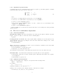
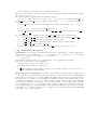
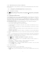
Representation of polynomials A variable or polynomial can only take values belonging to F3 =
{−1, 0, 1}. In Sigali, a polynomial is represented by means of a Ternary Decision Diagram(TDD) which
is an extension of a Binary Decision Diagram(BDD). In a TDD, each non-leaf node represents a variable
and each leaf node is a value of the polynomial. An arbitrary ordering of the variables must be done
to facilitate the assignment of a node to a variable. Further, each non-leaf node has 3 edges emanating
from it, labelled by the 3 possible values: {(-1 or 2), 0, 1} that the corresponding variable may take.
So, each path from the root to a leaf assigns a unique sequence of values to the variables and the value
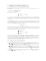
of the leaf gives the value of the polynomial for that particular assignment. For example, if p is the
polynomial a2 b + c2 , and the ordering is a < b < c, then p is represented by Sigali as follows (The TDD
representation of p is shown in Fig. 6.):
3
a
1, -1
0
b
0
1
-1
c
0
c
c
0
1, -1
1, -1
1, -1
-1
1
0
0
Figure 1: TDD representation of the polynomial a2 b + c2 .
Sigali : p : a^2 * b + c^2;
----------------------------------------------------------p
----------------------------------------------------------Sigali : p;
----------------------------------------------------------a=0
#0#
c=0
%0
c=1
%1
c=2
%1
c
a=1
#1#
b=0
subformula 0
b=1
c=0
%1
c=1
%2
c=2
%2
c
b=2
c=0
%2
c=1
%0
c=2
%0
c
b
a=2
subformula 1
a
-----------------------------------------------------------
In order to avoid repetitions in listing, portions occuring more than once are labelled as #n# (n = 0, 1,
2, ...). These repetitions tend to occur when two or more edges enter a non-leaf node in the TDD. While
reading the TDD, the label subformula n, wherever it occurs, is to be replaced by the portion labelled
#n#.
the command size(P); gives the number of nodes of the TDD that encodes the polynomial P.
Lists The list of polynomials, equations, etc. are written as follows: [a+b,c+d] is a list of polynomials
and [a+b=x,a*d^2=b^2] is an equation system. Of course, a symbol can be assigned to a list or an
equation system as well. For example:
• list :
[a + b, a, b, 0, 1];
• equations :
[a ^2 = b ^2, c = a and b];
4
If p is a polynomial, lp1 and lp2 are two lists of polynomials,lvar1 and lvar2 are two lists of variables,
and lconst is a list of constants(with values 0, 1 or -1), then:
• eval(p,[a,b,c],[0,1,-1]);
evaluates the polynomial p after substituting 0, 1 and -1 for a, b and c respectively. Of course
these variables must occur in p.
Note that we can use the command init lconst to declare the list of constants, e.g.
lconst : init lconst(3,0); is a list of 3 elements that are equal to 0, i.e. lconst=[0,0,0].
• rename(p, lvar1, lvar2);
replaces in p, the ith variable of lvar1 by the ith variable of lvar2.
• subst(p, lvar1, lp1);
replaces in p, the ith variable of lvar1 by the ith polynomial of lp1.
In case of the functions:
• l eval(lp1, lvar1, lconst);
• l rename(lp1, lvar1, lvar2);
• l subst(lp1, lvar1, lp2);
the first argument is a list of polynomials instead of one polynomial and they perform the same function
as their counterparts for each polynomial of the list.
1.2.4
(System of ) Polynomials manipulation
The canonical generator of a polynomial system given by a list of polynomials can be computed by the
function gen. The command is gen(lpoly); where lpoly is a list of polynomials. For example:
• gen([a + b - c, a^2 - 1]);
gives the canonical generator of the polynomial system given by the two polynomials a + b - c and a^2
- 1. The previous command can also be given as:
• gen([a + b = c, a^2 = 1]);
If P1 = a+b−c and P2 = a2 −1, then the previous command will compute the polynomial P = P1 ⊕P2 =
(P12 + P22 )2 , which entails that the solution of P will be the solution that are common to P1 and P2 .
• equal(p1,p2) compares two polynomials p1 and p2 and test whether they are equal or not.
Complementation. Let g be a polynomial and V its set of solutions, then the generator of the
complement of V is obtained by:
• complementary(g);
Intersection. Let p1 and p2 be two polynomials and V 1 and V 2 be the corresponding set of solutions,
then:
• intersection(p1,p2);
is the canonical generator of V1 ∩ V2 . The number of arguments can be greater than 2. For example one
can write intersection(p1,p2,p3,p4);
Union. Let p1 and p2 be two polynomials and V 1 and V 2 be the corresponding set of solutions, then:
• union(p1,p2);
is the canonical generator of V1 ∪ V2 . As in case of intersection, the number of arguments can be
greater than 2.
Tests of inclusion Let p1 and p2 be two polynomials and V 1 and V 2 be the corresponding set of
solutions, then:
• subset(g1,g2);
is True if and only if V1 ⊆ V2 .
5
1.2.5
Existential/universal variable elimination
Given a polynomial P over the variables X, Y , then we define the Existential/universal variable elimination as follows
• P’ : exist(Y,P) is a polynomial such that Sol(P 0 ) = {x|∃y, P (x, y) = 0}
• P’ : forall(X,P) is a polynomial such that Sol(P 0 ) = {x|∀y, P (x, y) = 0}
1.2.6
Automatic reordering
The set reorder(1) (exists also with the parameter 2) performs an automatic variable reordering using
heuristics. This is very useful to decrease the size of the TDD. set reorder(0) stops the automatic
reordering.
1.3
Systems and Processes
Sigali distinguishes between two categories of dynamical systems: systems and processes. Systems are
general dynamical systems in which null transitions (basically self loops) are taken into account even
when all the signals are absent, whereas in a process, null transitions are excluded i.e. No transition
can take place in the absence all the signals. Dynamical systems can be automatically derived from
either Signal programs or Matou programs thus allowing to allowing the modeling of reactive systems
by means of Mode Automata.
From a Signal/Matou programs, a file is automatically generated. it contains the following data:
• events is a list of variables encoding the event variables
• states is a list of variables which encodes the states variables
• controllables is a subset of events and corresponds to the controllable event variables (See section 3
for more details).
• evolutions is a list of polynomials (one for each state variables) which corresponds to the evolution
of each state variables.
• initialisations is a list of polynomials (the solutions of this polynomial systems correspond to the
initial states of the system).
• constraints is also a list of polynomial encoding the constraints part of the polynomial dynamical
system (i.e. Q(X, Y ) = 0).
If one want to construct from these sets a process (respectively a system), the following command has
to be used.
• syst :
processus(events,states,evolutions,initialisations,constraints,controllables);
Conversely, if syst is a dynamical system, as described by (3), constructed by the command system or
process, then the 6 components of syst can be accessed by:
• event var(syst); : returns the event variable set of a system, i.e. the vector Y
• state var(syst); : returns the state variable set of a system, i.e. the vector X
• evolution(syst); : returns the vector of polynomials encoding the evolution equations, i.e.
[P1 (X, Y ), · · · , Pn (X, Y )]
• initial(syst); : returns the polynomial encoding the initial states of the systems
• constraint(syst);: returns the constrains polynomial Q(X, Y )
• controllable var(syst); : returns the controllable variable set of a system, i.e. the vector U with
U ⊆ Y (See section 3 for more details).
1.3.1
Some special sets
If g is the canonical generator of a set of states E, then:
• pred(syst, g); is the canonical generator of the set of predecessors of E.
• all succ(syst, g); is the canonical generator of the set of states, such that all successors belong
to E.
6
• adm events(syst, g);is the canonical generator of the set of events admissible in E.
If g is the canonical generator of a set of events F , then:
• adm states(syst, g);
is the canonical generator of the set of states compatible with at least one of the events in F .
1.3.2
Implicit System
Starting from a system modeled as an PDS S as described in Equation System (3), for some particular
analysis, it is important to have access to the implicit corresponding implicit PDS of the form
R(X, Y, X 0 ) = 0
Qo (Xo ) = 0
(4)
The Sigali function that gives access to this new system is implicit sys(syst). The result is an I-PDS
(for implicit PDS). From a structure point of view, it is a 5-tuple (X, X 0 , Y, R, Q0 ) and the functions
that gives access to the components of this I-PDS are respectively state var I(), state var next I(),
event var I(), trans rel I(), initial I(), "controllable var I().
By loading the library Orbite.lib, you have access to the two following commands:
• P : Orbite(S Imp); returns the set of reachable states of the implicit system S Imp
• S 1:
1.4
Pruned((S Imp,Orbite); is an implicit Dynamical system, where all the states are reachable.
Fix-point Computation & Function definition
Fix point computation can also be performed. For example, given :
p0
pi+1
=
=
0
p2 + 1
the corresponding expression in Sigali is
loop x=x^2+1 init 0;
Of course, such sequences do not always converge. This is not checked by the system.
New function construction. Starting from the existing functions, it is also possible to define new
functions. The syntax is the following:
def f(x,y,z) :
with
intern 1 =
intern 2 =
do
Sigali body of the function
sigali expression,
sigali expression
;
For example, assume we want to compute the set of reachable states from Sol(P) in one step of an
implicit system SI . The corresponding function succ(P) is the following:
def succ(P) :
with
X = state_var_I(S_I),
X_Next = state_var_Next_I(S_I),
Y = event_var_I(Y),
Rel = trans_rel_I(S_I)
do
rename(exist(X, intersection(P,exist(Y, Rel)),X_Next,X));
7
1.5
Cost functions
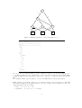
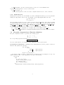
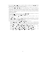
Sigali also offers the possibility to manipulate integers. Let X = (x1 , . . . , Xn ) be declared variables of
the system. Then, a cost function is a map from ( /3 )n to , which associates to each x = (x1 , · · · , xn )
of ( /3 )n some integer k. When f (x) is not defined then we assume that f (x) = ∞. To encode these
functions, we make the use of the ADD (Arithmetic decision diagrams). The ADD are similar to the
TDD expect that we attach integers to the leaves of the ADD. For example, let X < Y be two variables
in /3
and f a cost function such that
X
Y
f
0
0
3
0
1
2
0
-1
5
1
0
6
1
1
3
1
-1
4
-1
0
3
-1
1
8
-1
-1
3
Then the ADD that represents the function f is given by the graph of Figure 2 :
X1
1
-1
X2
3
0
X2
4
6
8
X2
3
3
2
5
3
Figure 2: Exemple d’un ADD
In order to build and manipulate cost functions, the following Sigali operations are available.
• a const(n) build the constant function equal to the integer n
• a var(X,n1,n2,n3): given a declared
cost function such that
X
X
X
variable X and 3 integers, f:
=
=
=
1
−1
0
⇔
⇔
⇔
ci (X)
ci (X)
ci (X)
=
=
=
a var(X,n1,n2,n3) build the
a
b
c
• Given two cost functions f1 and f2 , one can perform the sum and the product of f1 and f2 by
simply using the classical operators + and ∗.
• a min(f1,f2) is such that ∀x ∈ /3
• a max(f1,f2) is such that ∀x ∈ /3
n
, a min(f1 (x), f2 (x)) = min(f1 (x), f2 (x))
n
, a max(f1 (x), f2 (x)) = max(f1 (x), f2 (x))
• a part(P,f1,f2,f3 build a cost function such that a part(P,f1,f2,f3(x) = f1 if P(x)=0, f2 if
P(x)=1 and f3 if P(x)=-1
• a margmin(f,Y). given a cost function f defined over X ∪ Y , a margmin(f,Y) is a function, say f’
over the variables X such that f 0 (X) = minY (f (X, Y ), i.e. ∀y, f 0 (x) < f (x, y)
• a margmax (same as a margmin but with the max)
• P: a iminv(f,n) is a polynomial such that P (x) = 0 ⇔ f (x) = n
• a maxim(f) is the minimum value taken by f and a minim is the maximum value taken by f
• P: a inf(f,n) is a polynomial such that P (x) = 0 ⇔ f (x) ≤ n (a sup is also defined)
• R: a cost2rel(f1,f2). Given two cost functions over X1 and X2 (with the same cardinality)
a cost2rel(f1,f2) is a polynomial R(X1 , X2 ) such that R(x1 , x2 ) = 0 ⇔ f 1(x1 ) ≤ f 2(x).
2
Verification of systems using Sigali
Sigali provides certain functionalities for the verification of the properties of a dynamical system.
8
2.1
Liveness
Definition: A dynamical system is alive iff ∀x, y such that Q(x, y) = 0, ∃y 0 such that Q(P (x, y), y 0 ) =
0.
In other words, a system is alive iff it contains no sink states.
If syst is a system or a process, then:
• alive(syst);
is True if and only if syst is alive.
2.2
2.2.1
Safety Properties
Invariance
Definition: A set of states E is invariant for a dynamical system iff for every state x in E and every
event y admissible in x, the successor state x0 = P (x, y) is also in E.
If syst is a dynamical system and g is the canonical generator polynomial of a set of states E,
• invariant(syst, g);
is True if and only if E is invariant for syst.
For example, in case of the process double m, one can specify a property pr eq :
etat 2];. The invariance of this property can then be tested by the command:
[etat 1 =
• invariant(pf, gen(pr eq));,
where pf is the process constructed by the command system.
2.2.2
Invariance under control
Definition: A set of states E is control-invariant for a dynamical system iff for every state x in E,
there exists an event y such that Q(x, y) = 0 and the successor state x 0 = P (x, y) is also in E.
If syst is a dynamical system and g is the canonical generator polynomial of a set of states E,
• Invariant under control(syst, g);
is True if and only if E is control-invariant for syst.
2.2.3
Greatest (control-)invariant subset
Given a set of states E, there exists a set F 0 which is the greatest (control-)invariant subset of E. If syst
is a dynamical system and g is the canonical generator of E,then:
• greatest inv(syst, g);
• greatest c inv(syst, g);
gives the canonical generator of F 0 .
2.3
2.3.1
Reachability Properties
Reachability
Definition: A set of states E is reachable iff for every state x ∈ E there exists a trajectory starting
from the initial states that reaches x.
If syst is a dynamical system and g is the canonical generator polynomial of a set of states E,
• Reachable(syst, g);
is True if and only if E is reachable from the initial states of syst.
2.3.2
Attractivity
Definition: A set of states F is attractive for a set of states E iff every trajectory initialized on E
reaches F . If syst is a dynamical system and g is the canonical generator polynomial of a set of states
E,
• Attractivity(syst, g);
is True if and only if E is Attractive from the initial states of syst.
9
3
Synthesis of controllers using Sigali
3.1
Essentials of the control synthesis problem
For controllable polynomial dynamic systems, the set of events Y can be partitioned into two sets Y
and U , where,
• Y is the set of uncontrollable events,
• U is the set of controllable events.
The PDS can now be written as:
Q(X, Y, U )
X0
Q0 (X)
=
=
=
0
P (X, Y, U )
0
Let n, m, and p be the respective dimensions of X, Y , and U . The trajectories of a controlled system
are sequences (xt , yt , ut ) in (Z/3
Z ZZ )n+m+p such that Q0 (x0 ) = 0 and, for all t, Q(xt , yt , ut ) = 0 and
xt+1 = P (xt , yt , ut ). The events (yt , ut ) include an uncontrollable component yt and a controllable
component ut .
The controller: The PDS can be controlled by first selecting a particular initial state x0 and then
by choosing suitable values for u1 , u2 , .... Here, we only consider static control policies where the value
of the control ut is instantaneously computed from the value of xt and yt . Such a controller is called a
static controller. Formally, it is a system of two equations:
C(X, Y, U )
C0 (X)
=
=
0
0
where the latter equation determines the initial states satisfying the control objectives and the former
describes how to choose instantaneous controls. When the controlled system is in state x, and an event
y occurs, any value u such that Q(x, y, u) = 0 and C(x, y, u) = 0 can be chosen. The behavior of the
system composed with the controller is then modelled as:
Q(X, Y, U )
C(X, Y, U )
X0
Q0 (X)
C0 (X)
=
=
=
=
=
0
0
P (X, Y, U )
0
0
Control objectives ensuring properties like invariance, reachability, attractivity, etc are called traditional control objectives. There are also other kinds of control objectives which can be expressed as
partial order relations over the states of the PDS. These are called optimization control objectives.
Sigali provides functionalities for synthesis of controllers ensuring traditional as well as optimization
control objectives. There does not exist pre-existing Sigalifunctionalities. Instead, one have to load
different libraries in which Sigali functions are written.
3.2
Loading of the necessary libraries
For controller synthesis ensuring traditional control objectives, the Synthesis.lib file must be loaded.
• S c : S Invariance(S,prop); (or equivalently S Security(S,prop); If prop encodes a set of
states E, S Invariance(S,prop) computes a controller that ensures the invariance of E with respect
to the system S. The controlled system is the output of this function.
• S c : S Reachbale(S,prop); If prop encodes a set of states E, S Reachable(S,prop) computes
a controller that ensures the reachability of E from the initial states. The controlled system is the
output of this function. To ensure the attractivity, one have to use the S S Attractivity(S,prop);
command.
For dealing with optimization control objectives, two additional files: Synthesis Partial order.bib
and Synthesis Optimal Control.bib must also be loaded.
10
• The file Synthesis Partial Order.lib contains the definition of a function called S Free Max which
helps in choosing a control such that the system evolves, in the next instant, into a state where the
maximum number of uncontrollable events are admissible.
• The file Synthesis Partial Order Relation.lib contains function definitions for the synthesis of
optimal controllers. The goal is to synthesize a controller that will choose a control from amongst all
the admissible controls in such a way that the system evolves into a state according to a given choice
criterion. This criterion is expressed as a cost function relation on the set of states. Intuitively
speaking, the cost function is used to express priority between the different states that a system
can reach in one transition.
Technical Restiction
Input: C(X) is the cost function used for the control C Dup(X 1) is the duplicated cost function
of C(X) where X 1 is, for example obtained as follows:
Sigali> duplicate states : declare suff(state var(S));
next, one have to declare C Dup (i.e. same as for C but with the variables of the set
duplicate states
Nb.
No automatic reordering -> set reorder(0) the variable order must be as follows
X1>X1 1>X2>X2 1... So, if you plan to use the functions of this library then never use the
reodering after the use of declare suff(state var(S)) Once you plan not to use these functions anymore, then you activate again the automatic reordering.
The different functions of the Synthesis Partial Order Relation.lib are :
– Supervisor Lower than(S,C,C Dup,duplicate states) gives access to a controlled system
such that whatever the current position of the system S under control, the supervisor will
make the system evolve into the state x such that forall x0 reachable from the current position
C(x) ≤ C Dup(x0 ). Lower than(S,C,C Dup,duplicate states) build the controlled system.
– idem
for
Supervisor Greater than(S,C,C Dup,duplicate states)
and
Greater than(S,C,C Dup,duplicate states) (i.e. C(x) ≥ C Dup(x 0 )).
– idem
for
Supervisor Striclty Lower than(S,C,C Dup,duplicate states)
and
Striclty Lower than(S,C,C Dup,duplicate states) (i.e. C(x) < C Dup(x 0 )).
– idem
for
Supervisor Striclty Greater than(S,C,C Dup,duplicate states)
and
Striclty Greater than(S,C,C Dup,duplicate states) (i.e. C(x) > C Dup(x 0 )).
11