Download TPS User's Manual - Pages on gtps

TPS User’s Manual
Peter B. Andrews
Chad E. Brown
Matthew Bishop
Sunil Issar
Dan Nesmith
Frank Pfenning
Hongwei Xi
Mark Kaminski
R´
emy Chr´
etien
May 19, 2011
This material is based upon work supported by NSF grants MCS81-02870, DCR-8402532, CCR-8702699,
CCR-9002546, CCR-9201893, CCR-9502878, CCR-9624683, CCR-9732312, CCR-0097179, and a grant from
the Center for Design of Educational Computing, Carnegie Mellon University. Any opinions, findings, and
conclusions or recommendations are those of the authors and do not necessarily reflect the views of the National
Science Foundation.
ii
Contents
1 Introduction
1.1
Guide to documentation . . . . . . . . . . . . . . . . . . . . . . . . . . . . . . . . . . . . . . . . . .
1.2
The Tps User Interface . . . . . . . . . . . . . . . . . . . . . . . . . . . . . . . . . . . . . . . . . . .
1
1
1
2 Proving theorems
2.1
Introduction . . . . . . . . . . . . . . . . . . . . . . . . . . . . . . . . . . . .
2.2
Automatic mode . . . . . . . . . . . . . . . . . . . . . . . . . . . . . . . . .
2.2.1 An Example Using DIY . . . . . . . . . . . . . . . . . . . . . . . .
2.2.2 An Example Using MATE and ETREE-NAT . . . . . . . . . . . .
2.2.3 A Longer Example Using MATE and ETREE-NAT . . . . . . . .
2.2.4 Automatically Produced Proofs with Lemmas . . . . . . . . . . . .
ˆ ¡CR¿, G¡CR¿,
ˆ
2.2.5 Interrupts: C,
M¡CR¿ and T¡CR¿ . . . . . . . . . .
2.3
Interactive Mode . . . . . . . . . . . . . . . . . . . . . . . . . . . . . . . . .
2.3.1 Natural Deduction . . . . . . . . . . . . . . . . . . . . . . . . . . .
2.3.2 Extensional Sequent Calculus . . . . . . . . . . . . . . . . . . . . .
2.3.3 Manipulating Proofs . . . . . . . . . . . . . . . . . . . . . . . . . .
2.4
Combining Interactive and Automatic Searches . . . . . . . . . . . . . . . .
2.4.1 An Example Using Go to Start the Proof . . . . . . . . . . . . . .
2.4.2 Duplicating Interactively and then Running Matingsearch . . . . .
2.4.3 Applying Primsubs Interactively and then Running Matingsearch .
2.4.4 Mating Interactively and then Unifying . . . . . . . . . . . . . . .
2.4.5 Duplicating and Mating Interactively and then Converting to ND .
2.4.6 Using Prim-Single and Dup-Var Interactively . . . . . . . . . . . .
.
.
.
.
.
.
.
.
.
.
.
.
.
.
.
.
.
.
.
.
.
.
.
.
.
.
.
.
.
.
.
.
.
.
.
.
.
.
.
.
.
.
.
.
.
.
.
.
.
.
.
.
.
.
.
.
.
.
.
.
.
.
.
.
.
.
.
.
.
.
.
.
.
.
.
.
.
.
.
.
.
.
.
.
.
.
.
.
.
.
.
.
.
.
.
.
.
.
.
.
.
.
.
.
.
.
.
.
.
.
.
.
.
.
.
.
.
.
.
.
.
.
.
.
.
.
.
.
.
.
.
.
.
.
.
.
.
.
.
.
.
.
.
.
.
.
.
.
.
.
.
.
.
.
.
.
.
.
.
.
.
.
.
.
.
.
.
.
.
.
.
.
.
.
.
.
.
.
.
.
.
.
.
.
.
.
.
.
.
.
.
.
.
.
.
.
.
.
.
.
.
.
.
.
.
.
.
.
.
.
.
.
.
.
.
.
.
.
.
.
.
.
.
.
.
.
.
.
.
.
.
.
.
.
3
3
4
5
5
5
7
7
7
7
8
8
9
9
11
12
12
13
13
3 Setting and Varying Flags
3.1
Review, flags, and modes . . . . . . . . . . . . . . . . . . . . . . . .
3.2
Test: Multiple Searches on the Same Problem . . . . . . . . . . . .
3.2.1 How to Build A Searchlist Without Any Effort . . . . . .
3.2.2 Using TEST to Improve a Successful Mode . . . . . . . .
3.2.3 Using TEST to Discover a Successful Mode . . . . . . . .
3.2.4 Building A Searchlist with TEST . . . . . . . . . . . . . .
3.2.5 Uniform Search: Finding Successful Modes Automatically
3.3
Search Analysis: Facilities for Setting Flags and Tracing Automatic
3.3.1 Example: Setting Flags for THM12 . . . . . . . . . . . .
3.3.2 Example: Setting Flags for X2116 . . . . . . . . . . . . .
3.3.3 Tracing MS98-1 . . . . . . . . . . . . . . . . . . . . . . . .
3.3.4 Example: Tracing THM12 . . . . . . . . . . . . . . . . . .
3.3.5 Example: Tracing X2116 . . . . . . . . . . . . . . . . . .
.
.
.
.
.
.
.
.
.
.
.
.
.
.
.
.
.
.
.
.
.
.
.
.
.
.
.
.
.
.
.
.
.
.
.
.
.
.
.
.
.
.
.
.
.
.
.
.
.
.
.
.
.
.
.
.
.
.
.
.
.
.
.
.
.
.
.
.
.
.
.
.
.
.
.
.
.
.
.
.
.
.
.
.
.
.
.
.
.
.
.
.
.
.
.
.
.
.
.
.
.
.
.
.
.
.
.
.
.
.
.
.
.
.
.
.
.
.
.
.
.
.
.
.
.
.
.
.
.
.
.
.
.
.
.
.
.
.
.
.
.
.
.
.
.
.
.
.
.
.
.
.
.
.
.
.
.
.
.
.
.
.
.
.
.
.
.
.
.
15
15
16
16
16
17
17
20
21
21
22
24
25
29
4 How to define wffs, abbrevs, etc
. . . .
. . . .
. . . .
. . . .
. . . .
. . . .
. . . .
Search
. . . .
. . . .
. . . .
. . . .
. . . .
.
.
.
.
.
.
.
.
.
.
.
.
.
31
iv
5 Using the library
5.1
Storing and Retrieving Objects . . . .
5.2
Displaying Objects . . . . . . . . . . .
5.3
File Maintenance . . . . . . . . . . . .
5.4
Printed Output . . . . . . . . . . . . .
5.5
Expert Users . . . . . . . . . . . . . . .
5.6
Keywords . . . . . . . . . . . . . . . .
5.7
Classification Schemes . . . . . . . . .
5.8
The Unix-style Library Top Level . . .
5.9
Cautions . . . . . . . . . . . . . . . . .
5.10 How to insert TPTP Problems into the
CONTENTS
.
.
.
.
.
.
.
.
.
.
.
.
.
.
.
.
.
.
.
.
.
.
.
.
.
.
.
.
.
.
.
.
.
.
.
.
.
.
.
.
.
.
.
.
.
.
.
.
.
.
.
.
.
.
.
.
.
.
.
.
.
.
.
.
.
.
.
.
.
.
.
.
.
.
.
.
.
.
.
.
.
.
.
.
.
.
.
.
.
.
.
.
.
.
.
.
.
.
.
.
.
.
.
.
.
.
.
.
.
.
.
.
.
.
.
.
.
.
.
.
.
.
.
.
.
.
.
.
.
.
.
.
.
.
.
.
.
.
.
.
.
.
.
.
.
.
.
.
.
.
.
.
.
.
.
.
.
.
.
.
.
.
.
.
.
.
.
.
.
.
.
.
.
.
.
.
.
.
.
.
.
.
.
.
.
.
.
.
.
.
.
.
.
.
.
.
.
.
.
.
.
.
.
.
.
.
.
.
.
.
.
.
.
.
.
.
.
.
.
.
.
.
.
.
.
.
.
.
.
.
.
.
.
.
.
.
.
.
.
.
.
.
.
.
.
.
.
.
.
.
33
34
35
35
36
36
36
37
37
38
38
6 Mating Searches
6.1
Expansion trees and how they grow . . . . . . . . . . . .
6.2
The MATE Top-Level . . . . . . . . . . . . . . . . . . .
6.3
Primitive Substitutions . . . . . . . . . . . . . . . . . . .
6.3.1 How Primsubs are Generated . . . . . . . . . .
6.3.2 The MS91 Procedures . . . . . . . . . . . . . .
6.4
Some Important Flags in ms90-3 Search . . . . . . . . .
6.5
Helpful Hints for MS91 . . . . . . . . . . . . . . . . . . .
6.6
The Matingstree Procedure . . . . . . . . . . . . . . . .
6.6.1 A Brief Overview . . . . . . . . . . . . . . . . .
6.6.2 A Detailed Plan of the Matingstree Top Level .
6.6.3 How to Use the Mtree Top Level . . . . . . . .
6.6.4 Automatic Searches with the Mtree Top Level
6.6.5 The Mtree Subsumption Checker . . . . . . . .
6.6.6 An Interactive Session in the Mtree Top Level
.
.
.
.
.
.
.
.
.
.
.
.
.
.
.
.
.
.
.
.
.
.
.
.
.
.
.
.
.
.
.
.
.
.
.
.
.
.
.
.
.
.
.
.
.
.
.
.
.
.
.
.
.
.
.
.
.
.
.
.
.
.
.
.
.
.
.
.
.
.
.
.
.
.
.
.
.
.
.
.
.
.
.
.
.
.
.
.
.
.
.
.
.
.
.
.
.
.
.
.
.
.
.
.
.
.
.
.
.
.
.
.
.
.
.
.
.
.
.
.
.
.
.
.
.
.
.
.
.
.
.
.
.
.
.
.
.
.
.
.
.
.
.
.
.
.
.
.
.
.
.
.
.
.
.
.
.
.
.
.
.
.
.
.
.
.
.
.
.
.
.
.
.
.
.
.
.
.
.
.
.
.
.
.
.
.
.
.
.
.
.
.
.
.
.
.
.
.
.
.
.
.
.
.
.
.
.
.
.
.
.
.
.
.
.
.
.
.
.
.
.
.
.
.
.
.
.
.
.
.
.
.
.
.
.
.
.
.
.
.
.
.
.
.
.
.
.
.
.
.
.
.
.
.
.
.
.
.
.
.
.
.
.
.
.
.
.
.
.
.
.
.
.
.
.
.
.
.
.
.
.
.
.
.
.
.
.
.
.
.
.
.
.
.
.
.
.
.
.
.
.
.
.
.
.
.
.
.
.
.
.
.
.
.
.
.
.
.
.
.
.
.
.
.
.
.
.
.
.
.
.
.
.
.
.
.
41
41
41
42
42
45
46
47
47
47
48
50
51
51
52
7 Unification
7.1
A Few Comments About Higher-Order Unification
7.2
Bounds on Higher-Order Unification . . . . . . . .
7.2.1 Depth Bounds . . . . . . . . . . . . . . .
7.2.2 Substitution Bounds . . . . . . . . . . . .
7.2.3 Combining the Above . . . . . . . . . . .
7.3
Support Facilities . . . . . . . . . . . . . . . . . . .
7.3.1 Review . . . . . . . . . . . . . . . . . . .
7.3.2 Saving Disagreement sets . . . . . . . . .
7.4
Unification Tree . . . . . . . . . . . . . . . . . . . .
7.4.1 Node Names . . . . . . . . . . . . . . . .
7.4.2 Substitution Stack . . . . . . . . . . . . .
7.5
Simpl . . . . . . . . . . . . . . . . . . . . . . . . . .
7.6
Match . . . . . . . . . . . . . . . . . . . . . . . . .
7.7
Comments . . . . . . . . . . . . . . . . . . . . . . .
7.8
A Session in Unification Top-Level . . . . . . . . .
. . . . . . . .
. . . . . . . .
. . . . . . . .
. . . . . . . .
. . . . . . . .
. . . . . . . .
. . . . . . . .
. . . . . . . .
. . . . . . . .
Tps Library
.
.
.
.
.
.
.
.
.
.
.
.
.
.
.
.
.
.
.
.
.
.
.
.
.
.
.
.
.
.
.
.
.
.
.
.
.
.
.
.
.
.
.
.
.
.
.
.
.
.
.
.
.
.
.
.
.
.
.
.
.
.
.
.
.
.
.
.
.
.
.
.
.
.
.
.
.
.
.
.
.
.
.
.
.
.
.
.
.
.
.
.
.
.
.
.
.
.
.
.
.
.
.
.
.
.
.
.
.
.
.
.
.
.
.
.
.
.
.
.
.
.
.
.
.
.
.
.
.
.
.
.
.
.
.
.
.
.
.
.
.
.
.
.
.
.
.
.
.
.
.
.
.
.
.
.
.
.
.
.
.
.
.
.
.
.
.
.
.
.
.
.
.
.
.
.
.
.
.
.
.
.
.
.
.
.
.
.
.
.
.
.
.
.
.
.
.
.
.
.
.
.
.
.
.
.
.
.
.
.
.
.
.
.
.
.
.
.
.
.
.
.
.
.
.
.
.
.
.
.
.
.
.
.
.
.
.
.
.
.
.
.
.
.
.
.
.
.
.
.
.
.
.
.
.
.
.
.
.
.
.
.
.
.
.
.
.
.
.
.
.
.
.
.
.
.
.
.
.
.
.
.
.
.
.
.
.
.
.
.
.
.
.
.
.
.
.
.
.
.
.
.
.
.
.
.
.
.
.
.
.
.
.
.
.
.
.
.
.
.
.
.
.
.
.
.
.
.
.
.
.
.
.
.
.
.
.
.
.
.
.
.
.
.
.
.
.
.
.
.
.
.
.
.
.
.
.
.
.
.
.
.
.
.
.
.
.
.
.
.
.
.
.
.
.
.
.
.
.
.
.
.
.
.
.
.
.
.
.
.
.
.
.
.
.
.
.
.
.
.
57
57
57
58
58
59
59
59
59
59
60
60
60
60
61
61
8 Rewrite Rules and Theories
8.1
Top-Level Commands for Manipulating Rewrite Rules
8.2
Editor Operations Dealing with Rewrite Rules . . . . .
8.3
An Example of Rewrite Rules in Interactive Use . . . .
8.4
Using Rewrite Rules in Automatic Proof Search . . . .
8.5
The Rewriting Top Level . . . . . . . . . . . . . . . . .
8.5.1 Interacting with the Main Top Level . . . . .
8.5.2 Rewrite Rules, Theories and Derivations . . .
8.5.3 Automatic Search . . . . . . . . . . . . . . .
.
.
.
.
.
.
.
.
.
.
.
.
.
.
.
.
.
.
.
.
.
.
.
.
.
.
.
.
.
.
.
.
.
.
.
.
.
.
.
.
.
.
.
.
.
.
.
.
.
.
.
.
.
.
.
.
.
.
.
.
.
.
.
.
.
.
.
.
.
.
.
.
.
.
.
.
.
.
.
.
.
.
.
.
.
.
.
.
.
.
.
.
.
.
.
.
.
.
.
.
.
.
.
.
.
.
.
.
.
.
.
.
.
.
.
.
.
.
.
.
.
.
.
.
.
.
.
.
.
.
.
.
.
.
.
.
.
.
.
.
.
.
.
.
.
.
.
.
.
.
.
.
.
.
.
.
.
.
.
.
.
.
.
.
.
.
.
.
.
.
.
.
.
.
.
.
.
.
.
.
.
.
.
.
.
.
.
.
.
.
.
.
.
.
.
.
.
.
.
.
63
63
64
64
66
67
67
67
68
.
.
.
.
.
.
.
.
.
.
.
.
.
.
.
v
CONTENTS
8.6
8.5.4 Commands for Entering and Leaving the Rewriting Top Level . . . .
8.5.5 Commands for Starting, Finishing and Printing Rewrite Derivations
8.5.6 Commands for Applying Rewrite Rules . . . . . . . . . . . . . . . .
8.5.7 Commands for Rearranging the Derivation . . . . . . . . . . . . . .
8.5.8 Lambda Conversion Commands . . . . . . . . . . . . . . . . . . . . .
8.5.9 Commands Concerned with Rewrite Rules and Theories . . . . . . .
8.5.10 Applicable Commands from the Main Top Level . . . . . . . . . . .
8.5.11 Flags . . . . . . . . . . . . . . . . . . . . . . . . . . . . . . . . . . . .
8.5.12 Example . . . . . . . . . . . . . . . . . . . . . . . . . . . . . . . . . .
8.5.13 Semantics of Rewrite Rules . . . . . . . . . . . . . . . . . . . . . . .
How Rewrite Rules and Theories Are Stored in the Library . . . . . . . . . .
9 Proof Translations and Tactics
9.1
Translation between proof formats; tactics . . . . . . . . . . . . . .
9.1.1 Overview . . . . . . . . . . . . . . . . . . . . . . . . . . .
9.1.2 Syntax for Tactics and Tacticals . . . . . . . . . . . . . .
9.1.3 Tacticals . . . . . . . . . . . . . . . . . . . . . . . . . . . .
9.1.4 Using Tactics . . . . . . . . . . . . . . . . . . . . . . . . .
9.1.5 Translating from Natural Deduction to Expansion Proofs
.
.
.
.
.
.
.
.
.
.
.
.
.
.
.
.
.
.
.
.
.
.
.
.
.
.
.
.
.
.
.
.
.
.
.
.
.
.
.
.
.
.
.
.
.
.
.
.
.
.
.
.
.
.
.
.
.
.
.
.
.
.
.
.
.
.
.
.
.
.
.
.
.
.
.
.
.
.
.
.
.
.
.
.
.
.
.
.
.
.
.
.
.
.
.
.
.
.
.
.
.
.
.
.
.
.
.
.
.
.
.
.
.
.
.
.
.
.
.
.
.
.
.
.
.
.
.
.
.
.
.
.
.
.
.
.
.
.
.
.
.
.
.
.
.
.
.
.
.
.
.
.
.
.
.
.
.
.
.
.
.
.
.
.
.
.
.
.
69
69
70
70
71
71
71
71
72
74
75
.
.
.
.
.
.
.
.
.
.
.
.
.
.
.
.
.
.
.
.
.
.
.
.
.
.
.
.
.
.
.
.
.
.
.
.
.
.
.
.
.
.
.
.
.
.
.
.
.
.
.
.
.
.
.
.
.
.
.
.
.
.
.
.
.
.
.
.
.
.
.
.
77
77
77
78
80
81
81
10 Testing for Satisfiability
83
11 Output: Symbols, Files and Styles
11.1 Proofwindows . . . . . . . . . . . . . . . . .
11.2 Interpreting the Output from Mating Search
11.2.1 Symbols Printed by Mating Search
11.2.2 Refining the Output: the Monitor
11.3 Output files . . . . . . . . . . . . . . . . . .
11.4 Output styles . . . . . . . . . . . . . . . . .
11.5 Saving Output from Mating Search . . . . .
11.6 Interrupting TPS for Occasional Output . .
11.7 Output for Slides . . . . . . . . . . . . . . .
11.8 Record files . . . . . . . . . . . . . . . . . .
.
.
.
.
.
.
.
.
.
.
.
.
.
.
.
.
.
.
.
.
.
.
.
.
.
.
.
.
.
.
.
.
.
.
.
.
.
.
.
.
.
.
.
.
.
.
.
.
.
.
.
.
.
.
.
.
.
.
.
.
.
.
.
.
.
.
.
.
.
.
.
.
.
.
.
.
.
.
.
.
.
.
.
.
.
.
.
.
.
.
.
.
.
.
.
.
.
.
.
.
.
.
.
.
.
.
.
.
.
.
.
.
.
.
.
.
.
.
.
.
.
.
.
.
.
.
.
.
.
.
.
.
.
.
.
.
.
.
.
.
.
.
.
.
.
.
.
.
.
.
.
.
.
.
.
.
.
.
.
.
.
.
.
.
.
.
.
.
.
.
.
.
.
.
.
.
.
.
.
.
.
.
.
.
.
.
.
.
.
.
.
.
.
.
.
.
.
.
.
.
.
.
.
.
.
.
.
.
.
.
.
.
.
.
.
.
.
.
.
.
.
.
.
.
.
.
.
.
.
.
.
.
.
.
.
.
.
.
.
.
.
.
.
.
.
.
.
.
.
.
.
.
.
.
.
.
.
.
.
.
.
.
.
.
.
.
.
.
.
.
.
.
.
.
.
.
.
.
.
.
.
.
.
.
.
.
.
.
.
.
.
.
.
.
.
.
.
.
.
.
.
.
.
.
.
.
.
.
.
.
85
85
85
85
87
88
89
89
89
90
90
12 Events
12.1 Events in TPS . . . . . . . .
12.1.1 Defining an Event
12.1.2 Signalling Events .
12.1.3 Examples . . . . .
12.2 More on Events . . . . . . .
12.3 The Report Package . . . .
.
.
.
.
.
.
.
.
.
.
.
.
.
.
.
.
.
.
.
.
.
.
.
.
.
.
.
.
.
.
.
.
.
.
.
.
.
.
.
.
.
.
.
.
.
.
.
.
.
.
.
.
.
.
.
.
.
.
.
.
.
.
.
.
.
.
.
.
.
.
.
.
.
.
.
.
.
.
.
.
.
.
.
.
.
.
.
.
.
.
.
.
.
.
.
.
.
.
.
.
.
.
.
.
.
.
.
.
.
.
.
.
.
.
.
.
.
.
.
.
.
.
.
.
.
.
.
.
.
.
.
.
.
.
.
.
.
.
.
.
.
.
.
.
.
.
.
.
.
.
.
.
.
.
.
.
.
.
.
.
.
.
.
.
.
.
.
.
.
.
.
.
.
.
.
.
.
.
.
.
.
.
.
.
.
.
93
93
93
94
94
96
98
. . . . . .
. . . . . .
. . . . . .
own rules
. . . . . .
.
.
.
.
.
.
.
.
.
.
.
.
.
.
.
.
.
.
.
.
.
.
.
.
.
.
.
.
.
.
.
.
.
.
.
.
.
.
.
.
.
.
.
.
.
.
.
.
.
.
.
.
.
.
.
.
.
.
.
.
.
.
.
.
.
.
.
.
.
.
.
.
.
.
.
.
.
.
.
.
.
.
.
.
.
.
.
.
.
.
.
.
.
.
.
.
.
.
.
.
.
.
.
.
.
.
.
.
.
.
.
.
.
.
.
.
.
.
.
.
101
101
102
102
103
104
.
.
.
.
.
.
.
.
.
.
.
.
.
.
.
.
.
.
.
.
.
.
.
.
.
.
.
.
.
.
.
.
.
.
.
.
.
.
.
.
.
.
.
.
.
.
.
.
.
.
.
.
.
.
.
.
.
.
.
.
.
.
.
.
.
.
.
.
.
.
.
.
.
.
.
.
.
.
.
.
.
.
.
.
.
.
.
.
.
.
.
.
.
.
.
.
.
.
.
.
.
.
.
.
.
.
.
.
.
.
.
.
.
.
.
.
.
.
.
.
.
.
.
.
.
107
107
107
108
110
111
.
.
.
.
.
.
.
.
.
.
.
.
.
.
.
.
.
.
.
.
.
.
.
.
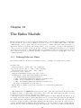
13 The Rules Module
13.1 Defining Inference Rules . . . . . .
13.2 Assembling the Rules . . . . . . . .
13.2.1 An example . . . . . . . .
13.2.2 Customizing Etps or Tps
13.2.3 Creating Exercises . . . .
.
.
.
.
.
.
.
.
.
.
.
.
.
.
.
.
.
.
. . .
. . .
. . .
with
. . .
.
.
.
.
.
.
.
.
.
.
.
.
. . .
. . .
. . .
your
. . .
14 Notes on setting things up
14.1 Compiling TPS and ETPS . . . . . . . . . . .
14.1.1 Compiling TPS under Unix . . . . .
14.1.2 Compiling TPS under MS Windows
14.1.3 Compiling the Java Interface . . . .
14.2 Initialization . . . . . . . . . . . . . . . . . . .
.
.
.
.
.
.
.
.
.
.
.
.
.
.
.
.
.
.
.
.
.
.
.
.
.
vi
CONTENTS
14.3
14.4
14.5
14.6
14.7
14.8
14.9
14.10
14.11
14.12
14.13
14.2.1 Initializing Tps . . . . . . . . . . . . . . . . . .
14.2.2 Initializing Etps . . . . . . . . . . . . . . . . .
Starting Tps . . . . . . . . . . . . . . . . . . . . . . . . .
Using Tps with the X window system . . . . . . . . . .
Using Tps with the Java Interface . . . . . . . . . . . . .
Using Tps within Gnu Emacs . . . . . . . . . . . . . . .
Running Tps in Batch Mode or from Omega . . . . . . .
14.7.1 Batch Processing Work Files . . . . . . . . . .
14.7.2 Interactive/Omega Batch Processing . . . . . .
14.7.3 Batch Processing With UNIFORM-SEARCH .
Calling Tps from Other Programs . . . . . . . . . . . . .
14.8.1 Establishing Connections . . . . . . . . . . . .
14.8.2 Socket Communication . . . . . . . . . . . . . .
14.8.3 Ping-Pong Protocol . . . . . . . . . . . . . . .
14.8.4 Requests . . . . . . . . . . . . . . . . . . . . . .
14.8.5 Example . . . . . . . . . . . . . . . . . . . . . .
Starting Tps as an Online Server . . . . . . . . . . . . .
14.9.1 Setting up the Online Server . . . . . . . . . .
14.9.2 Starting or Restarting the Online Server . . . .
Preparing ETPS for classroom use . . . . . . . . . . . .
14.10.1 Starting ETPS as an Online Server for a Class
14.10.2 Grades . . . . . . . . . . . . . . . . . . . . . . .
14.10.3 Security . . . . . . . . . . . . . . . . . . . . . .
14.10.4 Diagnosing Problems in ETPS . . . . . . . . .
Interruptions and Emergencies . . . . . . . . . . . . . . .
How to produce manuals . . . . . . . . . . . . . . . . . .
14.12.1 Scribe manuals . . . . . . . . . . . . . . . . . .
14.12.2 LATEX manuals . . . . . . . . . . . . . . . . . .
14.12.3 HTML manuals . . . . . . . . . . . . . . . . . .
Miscellaneous Information . . . . . . . . . . . . . . . . .
.
.
.
.
.
.
.
.
.
.
.
.
.
.
.
.
.
.
.
.
.
.
.
.
.
.
.
.
.
.
.
.
.
.
.
.
.
.
.
.
.
.
.
.
.
.
.
.
.
.
.
.
.
.
.
.
.
.
.
.
.
.
.
.
.
.
.
.
.
.
.
.
.
.
.
.
.
.
.
.
.
.
.
.
.
.
.
.
.
.
.
.
.
.
.
.
.
.
.
.
.
.
.
.
.
.
.
.
.
.
.
.
.
.
.
.
.
.
.
.
.
.
.
.
.
.
.
.
.
.
.
.
.
.
.
.
.
.
.
.
.
.
.
.
.
.
.
.
.
.
.
.
.
.
.
.
.
.
.
.
.
.
.
.
.
.
.
.
.
.
.
.
.
.
.
.
.
.
.
.
.
.
.
.
.
.
.
.
.
.
.
.
.
.
.
.
.
.
.
.
.
.
.
.
.
.
.
.
.
.
.
.
.
.
.
.
.
.
.
.
.
.
.
.
.
.
.
.
.
.
.
.
.
.
.
.
.
.
.
.
.
.
.
.
.
.
.
.
.
.
.
.
.
.
.
.
.
.
.
.
.
.
.
.
.
.
.
.
.
.
.
.
.
.
.
.
.
.
.
.
.
.
.
.
.
.
.
.
.
.
.
.
.
.
.
.
.
.
.
.
.
.
.
.
.
.
.
.
.
.
.
.
.
.
.
.
.
.
.
.
.
.
.
.
.
.
.
.
.
.
.
.
.
.
.
.
.
.
.
.
.
.
.
.
.
.
.
.
.
.
.
.
.
.
.
.
.
.
.
.
.
.
.
.
.
.
.
.
.
.
.
.
.
.
.
.
.
.
.
.
.
.
.
.
.
.
.
.
.
.
.
.
.
.
.
.
.
.
.
.
.
.
.
.
.
.
.
.
.
.
.
.
.
.
.
.
.
.
.
.
.
.
.
.
.
.
.
.
.
.
.
.
.
.
.
.
.
.
.
.
.
.
.
.
.
.
.
.
.
.
.
.
.
.
.
.
.
.
.
.
.
.
.
.
.
.
.
.
.
.
.
.
.
.
.
.
.
.
.
.
.
.
.
.
.
.
.
.
.
.
.
.
.
.
.
.
.
.
.
.
.
.
.
.
.
.
.
.
.
.
.
.
.
.
.
.
.
.
.
.
.
.
.
.
.
.
.
.
.
.
.
.
.
.
.
.
.
.
.
.
.
.
.
.
.
.
.
.
.
.
.
.
.
.
.
.
.
.
.
.
.
.
.
.
.
.
.
.
.
.
.
.
.
.
.
.
.
.
.
.
.
.
.
.
.
.
.
.
.
.
.
.
.
.
.
.
.
.
.
.
.
.
.
.
.
.
.
.
.
.
.
.
.
.
.
.
.
.
.
.
.
.
.
.
.
.
.
.
.
.
.
.
.
.
.
.
.
.
.
.
.
.
.
.
.
.
.
.
.
.
.
.
.
.
.
.
.
.
.
.
.
.
.
.
.
.
.
.
.
.
.
.
.
.
.
.
.
.
.
.
.
.
.
.
.
.
.
.
.
.
.
.
.
.
.
.
.
.
.
.
.
.
.
.
.
.
.
.
.
.
.
.
.
.
.
.
.
.
.
.
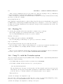
111
111
112
112
113
115
115
115
115
116
116
116
117
117
117
118
121
121
122
122
122
123
123
123
123
124
124
125
126
126
Bibliography
127
Index
130
Chapter 1
Introduction
Welcome to Tps, a theorem-proving environment developed at Carnegie Mellon University for both research
and education. Tps is based on the typed λ-calculus, and supports automatic, semi-automatic, and interactive
proofs of theorems of first- and higher-order logic.
For details on setting Tps up on your system, see chapter 14.
There are two subsystems of Tps which you may wish to use. The first, Etps, is an educational version
which is used in logic courses to prove theorems in purely interactive mode. It contains none of the automatic
features of Tps. The second, Grader, is a set of functions which are useful in keeping class grades, allowing, in
particular, the automatic processing of the record files created by Etps. There are separate manuals for each
of these systems. Grader is a part of Tps; you can enter the Grader top level via the command DO-GRADES.
1.1
Guide to documentation
At the present time, the Tps manuals are far from finished. Some areas are covered in detail, while others are
very sketchy. We hope, however, that these manuals will allow you to get started with Tps.
To first learn the system, read [35]. This will introduce you to the interaction style of the program, tell
you how to get help, and show you how to enter wffs and use the inference rules. Etps is used for educational
purposes, however, so it contains none of the automatic facilities of Tps such as mating-search.
For a full list of all commands, flags, etc., see [13]. Those relating to mating-search are in a separate chapter,
and other commands and flags can be found under the heading mating-search in other chapters.
There is also a programmer’s manual.
[28] covers the commands which are particular to the Grader subsystem.
Additional references which you may wish to consult are listed in the bibliography. [10] and [11] provide
general information about Tps. Some of the material in the latter paper was taken from this manual.
1.2
The Tps User Interface
Tps has various top levels. There is a main top level, and there are sub-top levels for specific purposes. Note
that the same command may be defined in more than one top level, and have different effects. In each top level,
the ? command will list all the commands available at that top level.
There are three interfaces for Tps: text-based, xterm-based, and Java-based. The first is purely text-based
and behaves as a lisp interpreter. The user types in text commands and Tps outputs a text response. To use
the xterm-based interface, one starts Tps inside a new xterm with special character fonts. The user also enters
commands as text, but the output can include special symbols (e.g., for logical operators and quantifiers). The
newest interface is a menu-based Java interface. With the Java interface the user can either type in a command
or choose the command from a menu. The output in the Java interface can also display special symbols such
as logical operators.
In any of these interfaces Tps can open new windows for special purposes. A common example is the use
of proofwindows for displaying different portions of the current proof. Using the command BEGIN-PRFW, the
2
CHAPTER 1. INTRODUCTION
user opens three new (xterm or Java) windows: the “Complete Proof” window, the “Current Subproof” window
and the “Current Subproof and Line Numbers” window.
The “Complete Proof” window displays the entire proof, and is useful when the proof is either short or one
wants a global view of the current state of a proof. At each stage in the construction of a natural deduction
proof, one unproved (or planned) proof line is the current goal, and certain lines, which must be processed to
derive it, are designated as support lines for that goal. The current goal and its supporting lines are displayed in
the “Current Subproof” window. The choice of these lines can be adjusted with the SUBPROOF, SPONSOR,
and UNSPONSOR commands. When the user applies a rule or tactic, the proofwindows are automatically
updated (under certain flag settings).
Another common use of auxiliary windows is in the EDITOR top level. This top level is used to manipulate
formulas. When the user enters this top level, a particular formula is given (either explicitly or implicitly, e.g.,
by giving the corresponding line number in the current natural deduction proof). Tps opens two new windows:
the “Top Edwff” window and the “Current Edwff” window. The user can issue commands to point to different
subformulas (which changes the contents of the “Current Edwff” window). If the user issues a command to
change the formula (e.g., INSTALL to instantiate abbreviations) the effect is to change the formula in the “Top
Edwff” window and the corresponding subformula in the “Current Edwff” window. In the EDITOR top level,
one can also give names (“weak labels”) to certain formulas which can later be used (in the same Tps session)
to refer to the formula. To save a formula permanently, one uses the library facilities (see Chapter 5).
Tps is also capable of creating TEX output. For example, the command TEXPROOF creates a TEX file
containing the current natural deduction proof (which may be partial or complete).
The user interface for Tps is the same as that for Etps. More information about it can be found in [12].
Chapter 2
Proving theorems
2.1
Introduction
Tps can be used to prove theorems automatically, interactively, or by using various combinations of automatic
and interactive facilities. Even if one is primarily interested in using it in automatic mode, one should consult
the ETPS User’s Manual [35] to learn the basics of interacting with both Etps and Tps. Even if one is
proving theorems purely interactively, one should probably use Tps rather than Etps so that one can use the
library facilities.
To start a proof in Tps, use the PROVE command. One can then develop the proof in natural deduction
style interactively, semi-automatically, or automatically.
To develop a proof in semi-automatic mode, one can alternate between applying rules of inference interactively, using a command called GO to apply rules suggested by Tps, using a command called GO2 to call a
number of tactics which quickly apply mundane rules of inference, and using the automatic facilities of Tps to
prove lemmas and to derive certain lines of the proof from other specified lines. One can develop parts of the
proof in whatever chronological order is most convenient. For example, one could start by inserting into the
proof the lines which represent the basic outline of a plan for the proof, and then work on filling in various parts
of this outline.
One can invoke the facilities for finding or completing the proof automatically with the DIY (“do it yourself”)
or DIY-L command. (The latter is used to fill in part of a proof, such as a proof of a lemma.) Before doing
this one should set various flags which control the search procedures. These flags play very important roles.
See chapter 3 for some information on how to set flags. The command PIY (“prove it yourself”) combines the
commands PROVE and DIY.
A set of flags and values for these flags is called a mode. If one does not know an appropriate mode when
one wishes to invoke Tps’s automatic procedures, one can use commands which systematically try a variety
of modes. A bestmode for a theorem is a mode which can be used to prove that theorem automatically (and
which will, in general, produce a proof more quickly than other modes). The Tps library contains certain sets
of modes called goodmodes such that each of the theorems which Tps can currently prove automatically can
be proven using at least one of the goodmodes in the set. For example, GOODMODES1 is a list of 68 modes,
and each of the 639 theorems for which bestmodes are currently saved can be proven automatically by at least
one of the modes in GOODMODES1. Using the command PIY2 (“Prove It Yourself, version 2”), DIY2, or
DIY2-L, one can direct Tps to apply its proof procedures with each of these 68 modes in turn for a specified
time, then increment the time limit and repeat the process, and continue in this way until a proof is found or
space or patience is exhausted. Since Tps can prove many theorems of moderate difficulty within a few seconds
(see [21, 19, 20, 9, 22, 23] for some examples), this makes Tps extremely convenient to use for filling in gaps of
moderate difficulty while one is constructing a major proof semi-interactively.
4
CHAPTER 2. PROVING THEOREMS
2.2
Automatic mode
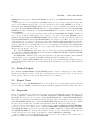
Automatic proof in Tps is based on the ‘mating-search’ paradigm described in [8], [4], and [6], or enhancements
of it described in [19, 20, 22, 23]. Tps starts by searching for an expansion proof [30, 31, 6] or an extensional
expansion proof [23], and then translates this into a natural deduction proof.
There are several ways in which one can use the automatic facilities of Tps.
The command DIY calls the mating-search facility (see Chapter 6), and if that succeeds in finding a proof,
applies a tactic (such as COMPLETE-TRANSFORM-TAC or PFENNING-TAC) to translate the expansion tree proof into
a natural deduction proof. Using DIY is the simplest way to prove a theorem automatically.
The nature of the search initiated by DIY or by GO will be heavily influenced by which setting you have for
the flag DEFAULT-MS. If you do setflag default-ms and then respond with ? when asked for an argument, you’ll
see the available options. Help messages will tell you a little about them, and there is some more information
in Chapter 6.
If you want to see more of what is going on in the search for a proof, you may want to start proving a theorem
by entering the MATE top-level with a particular wff and experimenting with the mating-search commands.
To do this, use the MATE command. See section 6 for information about this top-level.
After a mating has been found in the mating-search top-level and the expansion proof constructed, you can
apply the proper substitutions to the expansion tree with the MERGE-TREE command, which also eliminates
redundant branches from the tree. Or just use the LEAVE command, which will apply the merge procedure
and then return you to the main top-level. To build a natural deduction proof using the information in the
expansion proof you just constructed, use the command ETREE-NAT. You may also enter mating-search with
the most recent expansion proof created. This is stored in the variable CURRENT-EPROOF, and is the default value
for the MATE command. When you leave mating-search, this variable is set to the current expansion proof, so
you may reenter with the same proof if desired. The value of this variable is also the expansion proof used when
translating into a natural deduction proof with ETREE-NAT. Another variable, LAST-EPROOF, stores the value of
the expansion proof created before CURRENT-EPROOF. Either of these symbols may be entered when prompted
by the MATE command for a wff or eproof.
Details of how to save output from the mating search are in Chapter 11.
Let us discuss here exactly what the effects of the various mating search and translation commands are.
• The command MATE, when it returns to the top level, alters the value of the variable CURRENT-EPROOF
to be the expansion proof constructed.
• The command ETREE-NAT takes the expansion proof stored in CURRENT-EPROOF, places the information
it contains on the specified line of the natural deduction proof, then calls the specified tactic on the natural
deduction proof.
• The command DIY will construct an expansion proof for the specified planned line of the current natural
deduction proof, then, like ETREE-NAT, will place the information it contains on the specified line(s) of
the natural deduction proof and call the specified tactic. The value of CURRENT-EPROOF is not changed,
however.
Note that once the information from the expansion proof has been placed into the natural deduction proof,
as by DIY and ETREE-NAT, the value of CURRENT-EPROOF is unnecessary to the translation process, and one can
use the command USE-TACTIC to apply translation tactics. But since the MATE command does not transfer the
information fromn CURRENT-EPROOF into the natural deduction proof, the ETREE-NAT command must be applied
after MATE in order to start the translation process.
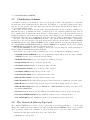
It is possible to translate natural deduction proofs to expansion proofs. This is accomplished by the command NAT-ETREE. The expansion proof created will be stored in the variable CURRENT-EPROOF. At present, this
procedure is not complete and will fail on some natural deduction proofs, including:
• Those which are not cut-free, i.e., do not satisfy the subformula property
• Those which use substitution of equality rules
• Those which use the assertion of axioms, like reflexivity of equality
5
2.2. AUTOMATIC MODE
2.2.1
An Example Using DIY
Comments are in italics.
<1>save-work workfile
We create a file called workfile.work which will record the commands used.
This is optional.
<2>prove theorem-name
We could also use the ‘exercise’ command if the theorem to be proved is
an exercise in ETPS.
<3>diy
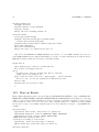
2.2.2
An Example Using MATE and ETREE-NAT
Alternatively, we may proceed as follows:
<1>save-work workfile
<2>prove theorem-name
<3>mate
<4>go
<5>merge-tree
You will be prompted for this when leaving the mate top level.
<6>etree-nat
To convert the proof to natural deduction style.
<7>daterec
To store the timing information in the library.
You may also want to go into the library to store a mode recording the
current flags.
<8>texproof
To produce printable output.
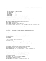
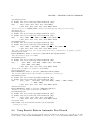
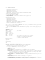
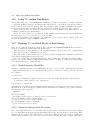
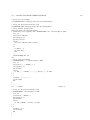
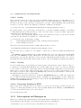
2.2.3
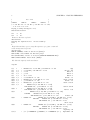
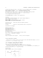
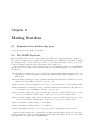
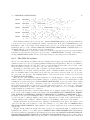
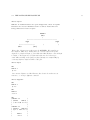
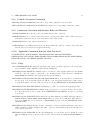
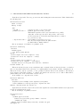
A Longer Example Using MATE and ETREE-NAT
To make the formulas easier to read, we have left off the type information. Note that ‘% f x’ denotes the image
of the set ‘x’ under the function ‘f’.
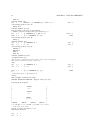
<8>exercise x5203
(100)
! % f [x INTERSECT y] SUBSET % f x INTERSECT % f y
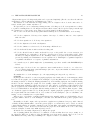
We call mating-search directly.
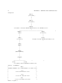
<9>mate
GWFF (GWFF0): gwff [No Default]>x5203
POSITIVE (YESNO): Positive mode [No]>!
We call the automatic proof search.
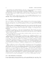
<Mate1>go
...
Displaying VP diagram ...
|
|
|
|
|
|
|
LEAF7
x T0
LEAF8
y T0
LEAF6
|
|
|
|
|
|
|
PLAN1
6
CHAPTER 2. PROVING THEOREMS
|
X0 = f T0
|
|
|
|LEAF12
LEAF13
LEAF15
LEAF16
|
|∼x t21 OR ∼X0 = f t21 OR ∼y t22 OR ∼X0 = f t22|
..*.+1.*.+2.*.+3.*.+4..
Trying to unify mating:(4 3 2 1)
Substitution Stack:
t21
->
T0
t22
->
T0..
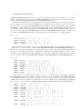
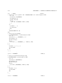
Return to the main top-level.
<Mate2>leave
Merging the expansion tree. Please stand by.
****
T
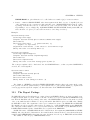
Begin the translation process using the expansion proof just constructed
in the mating-search top-level.
<9>etree-nat
PREFIX (SYMBOL): Name of the Proof [X5203]>
NUM (LINE): Line Number for Theorem [100]>
TAC (TACTIC-EXP): Tactic to be Used [COMPLETE-TRANSFORM-TAC]>
MODE (TACTIC-MODE): Tactic Mode [AUTO]>
We elide the output from the translation.
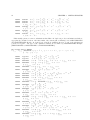
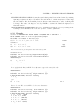
<0>pall
(1)
(2)
(3)
(4)
(5)
(88)
(89)
(93)
(94)
(95)
1
1,2
1,2
1,2
1,2
1,2
1,2
1,2
1,2
1,2
!
!
!
!
!
!
!
!
!
!
(96)
1
!
(97)
!
(98)
!
(99)
!
(100)
!
EXISTS t18 .x t18 AND y t18 AND x4 = f t18
Hyp
x t18 AND y t18 AND x4 = f t18
Choose: t18
x t18
RuleP: 2
y t18
RuleP: 2
x4 = f t18
RuleP: 2
x t18 AND x4 = f t18
RuleP: 3 5
EXISTS t19 .x t19 AND x4 = f t19
EGen: t18 88
y t18 AND x4 = f t18
RuleP: 4 5
EXISTS t20 .y t20 AND x4 = f t20
EGen: t18 93
EXISTS t19 [x t19 AND x4 = f t19]
AND EXISTS t20 .y t20 AND x4 = f t20
RuleP: 89 94
EXISTS t19 [x t19 AND x4 = f t19]
AND EXISTS t20 .y t20 AND x4 = f t20
RuleC: 1 95
EXISTS t18 [x t18 AND y t18 AND x4 = f t18]
IMPLIES
EXISTS t19 [x t19 AND x4 = f t19]
AND EXISTS t20 .y t20 AND x4 = f t20
Deduct: 96
FORALL x4 .
EXISTS t18 [x t18 AND y t18 AND x4 = f t18]
IMPLIES
EXISTS t19 [x t19 AND x4 = f t19]
AND EXISTS t20 .y t20 AND x4 = f t20
UGen: x4 97
FORALL x4 .
EXISTS t18 [x t18 AND y t18 AND x4 = f t18]
IMPLIES
EXISTS t19 [x t19 AND x4 = f t19]
AND EXISTS t20 .y t20 AND x4 = f t20
Equality: 98
% f [x INTERSECT y] SUBSET % f x INTERSECT % f y
EquivWffs: 99
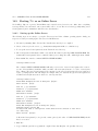
2.3. INTERACTIVE MODE
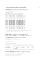
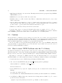
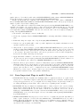
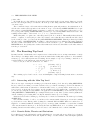
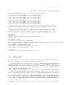
2.2.4
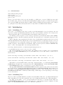
7
Automatically Produced Proofs with Lemmas
Some search procedures (e.g., using DIY when DEFAULT-MS is MS98-1 and DELAY-SETVARS is T) will
generate proofs which include lemmas which are asserted in the proofs. The proofs of these lemmas are also
generated and can be examined by using RECONSIDER. The name of the lemma is included with the Assert
justification. In general, PROOFLIST lists the names of all the natural deduction proofs in memory. An
example is the proof of THM2 produced using the mode EASY-SV-MODE.
2.2.5
ˆ ¡CR¿, G¡CR¿,
ˆ
Interrupts: C,
M¡CR¿ and T¡CR¿
During mating search, if the value of the flag INTERRUPT-ENABLE is T, you can interrupt the search by
typing <Return>. You will get a new mating-search (or matingstree, as appropriate) top-level, where you can
inspect and/or alter the current expansion tree and mating. Type LEAVE to return to mating-search.
Similarly, you can type ^
G<Return> (i.e. Control-G, then Return) to abandon the search for good and return
to the current top level. It is not possible to restart a search after doing this.
Lastly, you can type M<Return> to see the current mating, or T<Return> to see a printout of the time taken
so far by the search. The search will not be interrupted at all if you do this.
Of course, there is one, more drastic, way to interrupt a search: press ^
C. This will work regardless of the
setting of INTERRUPT-ENABLE, and will throw you into the Lisp debugger. Leaving the debugger with a
restart should return you to either the Tps top level or the current sub-toplevel; leaving it with a continue
should carry on the search.
For Allegro Common Lisp (debuggers are not standardized, so this will be different in other lisps), this works
as follows:
^
C
(control C)
Error: Received signal number 2 (Keyboard interrupt)
Restart actions (select using :continue):
0: continue computation
[1c] <cl>
Here one can use debugger commands,
or get into TPS on another level as follows:
[1c] <cl> (secondary-top-main)
Now do what you want in TPS to examine things.
To get back to the original TPS level:
<73>^
C
Error: Received signal number 2 (Keyboard interrupt)
Restart actions (select using :continue):
0: continue computation
1: continue computation
[2c] <cl> :cont 1
Now the original TPS process continues
Typing :res would have returned us to the TPS top level
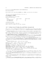
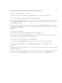
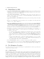
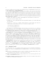
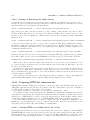
2.3
Interactive Mode
2.3.1
Natural Deduction
There are several examples showing how to construct natural deduction proofs completely interactively in
Chapter 4 of the ETPS User’s Manual [35]. Everything that can be done in Etps can also be done in Tps.
To prepare a demonstration of how to construct a proof interactively, use SAVE-WORK. To give the demonstration, use BEGIN-PRFW with the flags PROOFW-ACTIVE, PROOFW-ACTIVE+NOS or PROOFW-ALL
set to T, then use EXECUTE-FILE to give the demonstration; respond ‘yes’ to the ‘STEPPING?’ prompt. The
audience will see the proof being constructed step-by-step in the proofwindows. (Note: Stepping will only stop
between each command, so it will not stop (for example) between each step of GO2. Also, if you change top
level in a work file, stepping will be turned off until you return to the original top level. It is possible to force a
8
CHAPTER 2. PROVING THEOREMS
stop in these situations by inserting a PAUSE command into the workfile; see the help message for PAUSE for
more details.)
Alternatively, you may wish to go into MATE to prove the theorem automatically, then call ETREE-NAT
in interactive mode to demonstrate (with the aid of the proofwindows) how the natural deduction proof can be
constructed step-by-step. Make sure that the setting of ETREE-NAT-VERBOSE is appropriate before doing
this! (The user should note that if there is a command in the work file that changes the top level - for example,
BEGIN-PRFW or MATE - then this command will also turn off stepping. One can get around this limitation
by splitting the work file into two at the point where the change of top level occurs.)
While translating expansion proofs to natural deduction proofs, you may wish to set the flag TACMODE to
INTERACTIVE. See Section 9.1 for information on the effect of this flag. If you are using ETREE-NAT it is best
to call MERGE-TREE first; in fact, the mate top level will automatically prompt you for this if you attempt
to leave with a completed mating.
Equalities in expansion proofs can be translated into equational proofs as laid out in [34]. This does not
include the work on extensionality. In order to have the proper expansion proof transformation done during
merging, one should have the flag REMOVE-LEIBNIZ set to T, which is the default. It is also best to have
the flags REWRITE-EQUAL-EXT, REWRITE-EQUAL-EAGER, and REWRITE-ONLY-EXT set to NIL, and
REWRITE-EQUALITIES set to T.
From a Tps prompt (this could be either a top level prompt or the prompt produced by a command which
requires you to input some arguments) you can type PUSH to suspend what you’re doing and start a new top
level. The command POP will return from this top level to the point where you typed PUSH. For example,
you could suspend an interactive session with ETREE-NAT in order to print out the proof at various stages of
development.
It is also possible to interrupt an automatic search, change some flags and then continue with the search;
see section 2.2.5 for details.
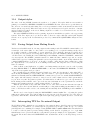
2.3.2
Extensional Sequent Calculus
There is a top level EXT-SEQ which provides an environment for constructing derivations of (one-sided) sequents
in the extensional sequent calculus described in [23]. The command ? will list all the available rules. Some
rules are basic while others are derived rules which can be expanded later. The cut rule is included, but certain
commands (namely, CUTFREE-TO-EDAG) will only work when given cut-free derivations.
The command GO2 in the top level EXT-SEQ will automatically suggest rules which are applicable. This
can make interactive construction of a sequent calculus derivation much easier.
Sequent derivations can be saved and restored using SAVEPROOF and RESTOREPROOF.
2.3.3
Manipulating Proofs
Tps has many facilities for manipulating proofs. There can be many proofs in memory at the same time, and
the command PROOFLIST lists the names of all the natural deduction proofs or extensional sequent derivations
currently in memory, along with the theorems they prove. One proof is designated as the current proof, and
one can change this with the RECONSIDER command. Proofs can be saved as files by SAVEPROOF, and
restored to memory by RESTOREPROOF.
CREATE-SUBPROOF creates a new proof consisting of specified lines of the current proof, plus all the
lines on which they depend. MERGE-PROOFS merges all of the lines of a subproof into the current proof.
TRANSFER-LINES copies specified lines of a subproof, and all lines on which they depend, into the current
proof.
Various commands (MOVE, DELETE, INTRODUCE-GAP, MODIFY-GAPS, RENUMBERALL, SQUEEZE)
are available for deleting or moving portions of a proof, changing the gaps in the numbers between lines, and
renumbering the lines. The CLEANUP command will delete all lines of a completed proof which are not actually
needed to prove the final line.
Sometimes one wishes to look at the main steps in a natural deduction proof without looking at all the
intermediate steps. The command BUILD-PROOF-HIERARCHY builds dependency information into a proof
so that the proof can be viewed as a hierarchy of subproofs. The command PBRIEF displays the proof lines
included in the top levels of this hierarchy to a depth specified by the user. When one asks Tps to EXPLAIN a
9
2.4. COMBINING INTERACTIVE AND AUTOMATIC SEARCHES
specified line in a proof, it displays in the same way the lines of the proof which are used to prove the specified
line. PRINT-PROOF-STRUCTURE displays the hierarchy itself in terms of the numbers of the proof lines.
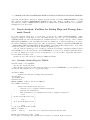
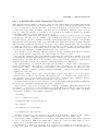
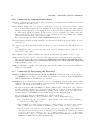
2.4
Combining Interactive and Automatic Searches
The command GO will apply inference rules based upon the structure of the formulas in the current proof
structure – breaking up conjunctions, applying the deduction rule, instantiating definitions, etc. This facility is
rather shallow, and requires the user to provide any terms for universal instantiation or existential generalization.
Thus while it may be useful in getting a proof started, it will eventually fail. The GO facility is fairly static as
well; to change the priority of the rules and/or keep some rules from being applied requires some programming
(see the file ml2-prior.lisp).
Tactics can also be used to do the same job. In this case, the user can build a tactic (see section 9.1) which
will apply inference rules in whatever order is desired. Tactics allow the user to experiment with different proof
strategies and express his or her own creative spirit. Tactics for applying most of the current inference rules are
already defined. See section 9.1.4 for more information on commands which invoke the most commonly used
tactics such as MONSTRO and GO2.
If a proof is being constructed interactively by natural deduction commands, it is possible to use the command
DIY-L to automatically complete some of the subproofs. This calls DIY to prove a lemma, adding lines to the
proof within a specified range. This is useful for quickly filling in the trivial parts of more difficult theorems
which you are proving interactively. See the help message for DIY-L for details. To keep the proof short and
readable, automatically-produced subproofs need not be translated completely; see the help message of the flag
USE-DIY for more information about this.
The tactic DIY-TAC basically just calls the DIY command, and thus can be used in tactics which first do some
manipulation of the proof based upon the structure of the formulas, then call mating-search when instantiations
of quantifiers must be found. (Note: if the flag USE-DIY is set, the translation may simply consist of justifying
the goal line as ‘Automatic’ from the support lines. This is useful for keeping the proof short.)
We now give several examples of how to start a proof interactively and continue automatically. Note that
if you modify the expansion tree interactively, you should use the command CJFORM before attempting to
construct a mating interactively.
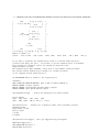
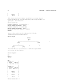
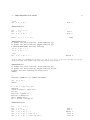
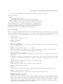
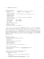
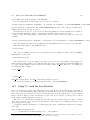
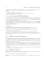
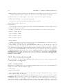
2.4.1
An Example Using Go to Start the Proof
<3>exercise x5203
(100)
! % f [x INTERSECT y] SUBSET % f x INTERSECT % f y
We use the GO command to start the proof.
<4>go
Considering planned line 100.
IDEF 100
Command [(IDEF 100)]>
Instantiate the definition of SUBSET.
(99)
! FORALL x .
% f [x INTERSECT y] x
IMPLIES [% f x INTERSECT % f y] x
Considering planned line 99.
The first two occurrences of x have different types, but they are not shown.
UGEN 99
Command [(UGEN 99)]>
(98)
! % f [x INTERSECT y] x IMPLIES [% f x INTERSECT % f y] x
Considering planned line 98.
DEDUCT 98
Command [(DEDUCT 98)]>
(1)
1
! % f [x INTERSECT y] x
(97) 1
! [% f x INTERSECT % f y] x
Considering planned line 97.
EDEF 1
PLAN1
PLAN2
PLAN3
Hyp
PLAN4
10
CHAPTER 2. PROVING THEOREMS
IDEF 97
Command [(EDEF 1)]>
(2)
1
! EXISTS t .[x INTERSECT y] t AND x = f t
Considering planned line 97.
RULEC 97 2
Command [(RULEC 97 2)]>
Some defaults could not be determined.
y (GWFF): Chosen Variable Name [No Default]>’’t’’
(3)
1,3
! [x INTERSECT y] t AND x = f t
(96) 1,3
! [% f x INTERSECT % f y] x
Considering planned line 96.
ECONJ 3
Command [(ECONJ 3)]>
(4)
1,3
! [x INTERSECT y] t
(5)
1,3
! x = f t
Considering planned line 96.
SUBST=L 5
SUBST=R 5
EDEF 4
IDEF 96
Command [(SUBST=L 5)]>^
G
‘[Command aborted.]’
We abort the command because the advice doesn’t seem very helpful.
Here are the current active lines of the proof.
<5>^
p
(4)
1,3
! [x INTERSECT y] t
(5)
1,3
! x = f t
...
(96) 1,3
! [% f x INTERSECT % f y] x
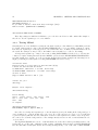
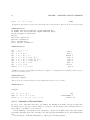
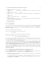
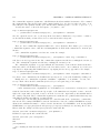
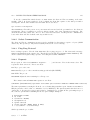
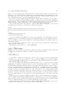
T
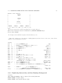
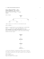
Call mating-search on the partial proof.
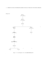
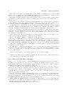
<6>diy
GOAL (PLINE): Planned Line [96]>
SUPPORT (EXISTING-LINELIST): Support Lines [(4 5)]>
...
Displaying VP diagram ...
|
LEAF88
|
|
x t
|
|
|
|
LEAF89
|
|
y t
|
|
|
|
LEAF90
|
|
x = f t
|
|
|
|LEAF96
LEAF97
LEAF99
LEAF100 |
|∼x t16 OR ∼x = f t16 OR ∼y t17 OR ∼x = f t17|
..*.+1.*.+2.*.+3.*.+4..
Trying to unify mating:(4 3 2 1)
Substitution Stack:
t16
t17
->
->
t
t.
Defn: 1
Choose: t
PLAN7
Conj: 3
Conj: 3
Conj: 3
Conj: 3
PLAN7
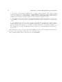
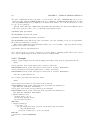
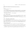
2.4. COMBINING INTERACTIVE AND AUTOMATIC SEARCHES
11
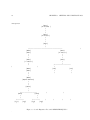
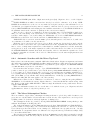
Eureka! Proof complete..
|
LEAF88
|
|
x t
|
|
|
|
LEAF89
|
|
y t
|
|
|
|
LEAF90
|
|
x = f t
|
|
|
|LEAF96
LEAF97
LEAF99
LEAF100 |
| ∼x t OR ∼x = f t OR ∼y t OR ∼x = f t|
****
A proof was found and now will be translated back to natural deduction.
What tactic should be used for translation? [COMPLETE-TRANSFORM-TAC]>
Tactic mode? [AUTO]>
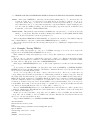
For brevity we have elided the output from the translation process.
Here’s the complete proof. Note that it is slightly different from that shown in section 2.2.3, where all the
definitions were instantiated at one time.
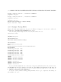
<7>pall
(1)
1
(2)
1
(3)
1,3
(4)
1,3
(5)
1,3
(6)
1,3
(7)
1,3
(8)
1,3
(88) 1,3
(89) 1,3
(93) 1,3
(94) 1,3
(95) 1,3
!
!
!
!
!
!
!
!
!
!
!
!
!
(96)
(97)
(98)
!
!
!
1,3
1
(99)
!
(100)
!
2.4.2
% f [x INTERSECT y] x
Hyp
EXISTS t .[x INTERSECT y] t AND x = f t
Defn: 1
[x INTERSECT y] t AND x = f t
Choose: t
[x INTERSECT y] t
Conj: 3
x = f t
Conj: 3
x t AND y t
EquivWffs: 4
x t
RuleP: 6
y t
RuleP: 6
x t AND x = f t
RuleP: 5 7
EXISTS t14 .x t14 AND x = f t14
EGen: t 88
y t AND x = f t
RuleP: 5 8
EXISTS t15 .y t15 AND x = f t15
EGen: t 93
EXISTS t14 [x t14 AND x = f t14]
AND EXISTS t15 .y t15 AND x = f t15
RuleP: 89 94
[% f x INTERSECT % f y] x
EquivWffs: 95
[% f x INTERSECT % f y] x
RuleC: 2 96
% f [x INTERSECT y] x IMPLIES [% f x INTERSECT % f y] x
Deduct: 97
FORALL x .
% f [x INTERSECT y] x
IMPLIES [% f x INTERSECT % f y] x
UGen: x 98
% f [x INTERSECT y] SUBSET % f x INTERSECT % f y
Defn: 99
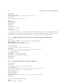
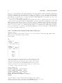
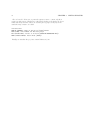
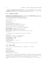
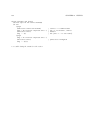
Duplicating Interactively and then Running Matingsearch
<11>mate
GWFF (GWFF0-OR-EPROOF): Gwff or Eproof [No Default]>thm-name
DEEPEN (YESNO): Deepen? [Yes]>
WINDOW (YESNO): Open Vpform Window? [No]>
12
CHAPTER 2. PROVING THEOREMS
<Mate12>vp
<Mate13>goto leaf58
This should be the name of the literal you wish to duplicate.
<Mate14>up
Go to the appropriate expansion node.
EXP8
<Mate18>vp
<Mate19>dup-var
<Mate21>dp*
<Mate23>∧
<Mate24>vp
To check we got it right...
<Mate27>go
To start matingsearch.
Users who are planning to both duplicate and Skolemize interactively should note that duplication and
Skolemization are not interchangeable. If you duplicate first and then Skolemize you will get different Skolem
functions, whereas if you Skolemize and then duplicate you will get the same Skolem function twice.
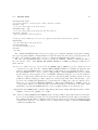
2.4.3
Applying Primsubs Interactively and then Running Matingsearch
<23>mate
GWFF (GWFF0-OR-EPROOF): Gwff or Eproof [No Default]>thm-name
DEEPEN (YESNO): Deepen? [Yes]>
WINDOW (YESNO): Open Vpform Window? [No]>
<Mate24>name-prim
We see that PRIM1 is the term we want to use.
<Mate25>vp
This will show the variable name we want. Note that pdeep and psh may
not show the right variable; things get renamed!
<Mate26>prim-single
TERM (GWFF): [No Default]>prim1
VAR (GWFF): [No Default]>‘R^3(OII)’
<Mate27>vp
Just to check...
<Mate28>go
2.4.4
Mating Interactively and then Unifying
<Mate24>cjform
<Mate25>vp
We do this because the leaf names may have changed.
<Mate26>add-conn*
Now we type in a whole list of connections; we could also have used add-conn.
Suppose we now think we have a complete mating...
<Mate27>complete-p
Mating is complete.
<Mate28>unify
We enter the unification top level; this only works for higher-order problems.
<Unif29>go
In case TPS halts with the message
MORE
you can proceed as follows:
2.4. COMBINING INTERACTIVE AND AUTOMATIC SEARCHES
<Unif30>MAX-UTREE-DEPTH
MAX-UTREE-DEPTH [20]>30
<Unif31>go
2.4.5
Duplicating and Mating Interactively and then Converting to ND
<66>mate
<Mate67>vp
<Mate68>goto leaf58
<Mate69>up
<Mate73>vp
<Mate74>dup-var
<Mate76>dp*
<Mate78>^
<Mate79>vp
<Mate80>add-conn leaf29 leaf58
...as often as needed to get the mating...
<Mate88>complete-p
<Mate89>show-mating
<Mate90>show-substs
<Mate91>vp
<Mate92>leave
Merge the expansion tree? [Yes]>
<93>etree-nat
2.4.6
Using Prim-Single and Dup-Var Interactively
<8>mate
We should check some flags before proceeding:
<Mate10> PRIM-BDTYPES
<Mate11>MIN-PRIM-DEPTH
<Mate12>MAX-PRIM-DEPTH
<Mate13> PRIM-QUANTIFIER
<Mate16>vp
<Mate17>NAME-PRIM
<Mate24>PRIM-SINGLE
SUBST (GWFF): [No Default]>prim14
VAR (GWFF): [No Default]>‘M^0(O(II))’
<Mate25>vp
<Mate30>etd
<Mate31>goto
NODE (SYMBOL): [No Default]>exp2
<Mate33>dup-var
<Mate35>dp*
<Mate37>^
<Mate38>vp
<Mate39>add-conn*
<Mate40>complete-p
We should check some flags before proceeding:
<Mate42>MAX-SEARCH-DEPTH
<Mate43>MAX-UTREE-DEPTH
<Mate44>unify
<Unif45>go
<Unif47>leave
13
14
<Mate48>leave
Merge the expansion tree? [Yes]>
<50>etree-nat
<51>pall
...to see the final proof.
CHAPTER 2. PROVING THEOREMS
Chapter 3
Setting and Varying Flags
The settings of flags are very important during automatic search. For example, flags like REWRITE-DEFNS
and REWRITE-EQUALITIES must be set to T (true) if you want definitions and equalities, respectively, to be
rewritten when the expansion tree is created from the formula to be proved. To see all of the flags which will
affect mating-search, check the facilities guide.
Since there are many flags in Tps, the flags which are most crucial to mating search have been collected
together under the subject IMPORTANT, so that typing LIST IMPORTANT will produce a list of the settings
of the dozen or so most important flags for mating search.
Tps has a facility called UNIFORM-SEARCH, which attempts to find the correct flag settings on its own;
it is capable of finding correct settings for many of the theorems which Tps has proven to date. See section 3.2
for more details.
3.1
Review, flags, and modes
The Review top-level is provided to make it easier to update flag-settings. Enter the top-level with the command
REVIEW. The commands provided in this top-level (for a listing, enter ?) give information about the various
flags available. Each flag is listed under one or more subjects. You may use the command SETFLAG to change
the value of a flag, or you may simply type the name of the flag itself. When entering the argument for a flag,
you may type ?? for more information about the argument type. In some cases, Tps will warn the user that the
flag is irrelevant, given the settings of other flags. File names and extensions should be entered as strings (i.e.
surrounded by double quotes); although in some circumstances one can omit the quotes, it is never an error to
include them.
All the flags for a subject can be listed by using the LIST command; help list will tell you more. You
may search the help messages of flags by using the KEY command; for example key ‘unification’ all will
find the flags whose help messages mention unification, in all subjects. A similar command SEARCH allows
you to search the help messages of all Tps objects.
To update many flags at once, use UPDATE or UPDATE-RELEVANT. The UPDATE commmand allows
the user to set all the flags in given subjects. Since certain flag values render some other flags irrelevant, there is
a command called UPDATE-RELEVANT which allows users to conveniently take into account the relationships
between flags and the decisions previously made while setting flags interactively. Since proof procedures are
constantly being developed or refined, when UPDATE-RELEVANT is called, the user is given the option of
using the current flag relevancy information in memory, loading flag relevancy information which has been saved
to a file, or rebuilding flag relevancy information automatically by processing the Lisp source files.
Modes are collections of flags with specified settings. By selecting a mode, you simultaneously set all the
included flags. You can also define your own modes and save them. See the INSERT command, in the library
top level, for more information.
See section 3.3 for information on how to use a known proof to suggest Tps flag settings, and Chapter 6 for
information about certain flags which affect the search processes.
Currently defined flags and modes are listed in the facilities guide [14].
16
3.2
CHAPTER 3. SETTING AND VARYING FLAGS
Test: Multiple Searches on the Same Problem
The TEST top level is designed to allow a succession of searches with varying flag settings to be performed
without any interaction from the user.
One of the major uses of this top level is to find settings of the various flags which will produce a proof of a
theorem; this is done by the UNIFORM-SEARCH command, which is explained later in section 3.2.5.
The top level is entered with the TEST command; as with the mate top level, this will prompt for a gwff
and ask whether you want to open a vpwindow.
There are three major groups of TEST commands; those which are for specifying a list of flags to be varied,
those which deal with the associated library functions and those which actually perform the search.
There is one major new data structure: a searchlist is a list of search items; each search item contains the
name of a flag, a default (initial) value for the flag, and a range of values over which it should be varied. The user
can have several searchlists in memory at once, and can switch between them with the NEW-SEARCHLIST
command. See below for an example of how to construct a searchlist. Searchlists can be stored in the library
with the INSERT command (from the test top level), and retrieved with the FETCH command (also from the
test top level). There is an additional (optional) function attached to each searchlist; this will be called on
each iteration of the search, and may do such things as setting flags which are not in the searchlist (so, for
example, MAX-SEARCH-DEPTH and MAX-UTREE-DEPTH can be kept equal to each other by having one
in the searchlist and the other set by the optional function). The function UNIFORM-SEARCH-FUNCTION
is used by the UNIFORM-SEARCH procedures.
The searchlist also contains (invisible to the user) internal flags which determine the current position in the
search; this means that it is possible to interrupt a search, save the current searchlist in the library, and later
on to reload that searchlist (even into a different core image) and continue the search from the point where it
was interrupted.
Once a searchlist is constructed, the GO command will start a search and the CONTINUE command will
continue a search after an interruption. The flags in the subject test-top control many of the parameters of the
search; type list test-top for more information. The user has the option of opening a test-window, analogous
to the vpwindow, which will show a summary of the search so far. If the search finds a proof, it will terminate;
otherwise, it will increase the time limit in the flag TEST-INITIAL-TIME-LIMIT and try again. Once the
search terminates, it will define a new mode which can be saved in the library using INSERT from the test top
level. (The INSERT in the library top level is different; when you try to save a mode, it asks you to specify all
the flag settings. The INSERT in the test top level merely asks for the name of the mode.)
3.2.1
How to Build A Searchlist Without Any Effort
The commands VARY-MODE and QUICK-DEFINE are useful for defining searchlists quickly. The former takes
an existing mode, and steps through it flag by flag, building a searchlist by offering to add each flag of the mode
and an appropriate range to the new searchlist. The latter uses a pre-defined list of flags, either those listed in
the TEST-FASTER-* group or those listed in the TEST-EASIER-* group, to create a searchlist in which each
of the flags has up to TEST-MAX-SEARCH-VALUES possible values.
Given a large searchlist, it is possible to trim it down using the SCALE-UP and SCALE-DOWN commands;
for each of the flags in the TEST-EASIER-* or TEST-FASTER-* lists (respectively), these commands compare
the range of the flags in the searchlist with the current values of the flags, and remove all values that would not
make the search easier (in the case of SCALE-UP) or faster (in the case of SCALE-DOWN).
In some cases, it is not necessary to build a searchlist at all. The commands PRESS-DOWN, PUSH-UP
and FIND-BEST-MODE all build their own searchlists using the flags listed in the TEST-FASTER-* flags (for
PRESS-DOWN and FIND-BEST-MODE) and those listed in the TEST-EASIER-* flags (for PUSH-UP and
FIND-BEST-MODE). Below are examples of how to use these commands.
3.2.2
Using TEST to Improve a Successful Mode
<18>test sample-theorem !
<test19>mode mode-sample-theorem
mode-sample-theorem is a mode in which sample-theorem can be proven.
3.2. TEST: MULTIPLE SEARCHES ON THE SAME PROBLEM
<test20>list test-top
Subject: TEST-TOP
TEST-FASTER-IF-HIGH:
TEST-FASTER-IF-LOW:
(MIN-QUICK-DEPTH)
(MAX-SEARCH-DEPTH SEARCH-TIME-LIMIT MAX-UTREE-DEPTH
MAX-MATES MAX-SEARCH-LIMIT)
TEST-FASTER-IF-NIL:
()
TEST-FASTER-IF-T:
(MIN-QUANTIFIER-SCOPE MS-SPLIT)
TEST-FIX-UNIF-DEPTHS: T
TEST-INCREASE-TIME:
0
TEST-INITIAL-TIME-LIMIT: 30
TEST-MAX-SEARCH-VALUES: 10
TEST-REDUCE-TIME:
T
Some flags have been omitted. When we do PRESS-DOWN, it will
automatically create a searchlist which will vary each
of the flags listed in the TEST-FASTER-* flags above, and then
start searching with a maximum time of 30 seconds, decreasing the
time as it goes, and fixing the unification depths after the
first successful search.
<test21>press-down
The search is started. While it works, we can go away for a
cup of coffee (or a two-week vacation to Mexico, depending on how
difficult sample-theorem is).
3.2.3
Using TEST to Discover a Successful Mode
<18>test sample-theorem !
<test19>mode bad-mode
bad-mode is a mode in which sample-theorem cannot be proven.
<test20>list test-top
Subject: TEST-TOP
TEST-EASIER-IF-HIGH:
(MAX-SEARCH-DEPTH SEARCH-TIME-LIMIT NUM-OF-DUPS
MAX-UTREE-DEPTH MAX-MATES MAX-SEARCH-LIMIT)
TEST-EASIER-IF-LOW:
(MIN-QUICK-DEPTH)
TEST-EASIER-IF-NIL:
()
TEST-EASIER-IF-T:
(ETA-RULE MIN-QUANTIFIER-SCOPE MS-SPLIT)
TEST-INCREASE-TIME:
10
TEST-INITIAL-TIME-LIMIT: 30
TEST-MAX-SEARCH-VALUES: 10
Some flags have been omitted. When we do PUSH-UP, it will
automatically create a searchlist which will vary each
of the flags listed in the TEST-EASIER-* flags above, and then
start searching with a maximum time of 30 seconds, increasing the
time by ten percent on each attempt.
<test21>push-up
The search is started. It will stop as soon as it finds a mode which works.
We can combine both PUSH-UP and PRESS-DOWN (first push-up to find a successful
mode, then press-down to find a better mode) by using the command FIND-BEST-MODE
instead of PUSH-UP.
3.2.4
Building A Searchlist with TEST
<12>list test-top
17
18
CHAPTER 3. SETTING AND VARYING FLAGS
Subject: TEST-TOP
TEST-INITIAL-TIME-LIMIT: 30
TEST-NEXT-SEARCH-FN:
EXHAUSTIVE-SEARCH
TEST-REDUCE-TIME:
T
TEST-VERBOSE:
T
TESTWIN-HEIGHT:
24
TESTWIN-WIDTH:
80
These are the flags available. Note the first three; the first says that
each search will be allowed 30 seconds, the second that the function
EXHAUSTIVE-SEARCH will be used to determine which flag settings are used next,
and the third that if a proof is found, the time allowed for the next proof
will be decreased.
<13>test
GWFF (GWFF0-OR-EPROOF): Gwff or Eproof [No Default]>x5305
DEEPEN (YESNO): Deepen? [Yes]>
WINDOW (YESNO): Open Vpform Window? [No]>yes
File to send copy Vpform output to (‘‘ ’’ to discard) [‘‘vpwin.vpw’’]>‘‘test-top.vpw’’
Use CLOSE-MATEVPW when you want to close the vpwindow.
<test14>?
Top Levels:
LEAVE
Mating search: CLOSE-TESTWIN CONTINUE GO OPEN-TESTWIN SEARCH-ORDER
Searchlists:
ADD-FLAG ADD-FLAG* ADD-SUBJECTS NEW-SEARCHLIST REM-FLAG
REM-FLAG* SEARCHLISTS SHOW-SEARCHLIST
Library:
DELETE FETCH INSERT
<test15>new-searchlist
NAME (SYMBOL): Name of new searchlist [No Default]>x5305-search
We begin to define a new searchlist, containing the flags to be varied.
<test16>searchlists
X5305-SEARCH
...this is currently the only searchlist in memory...
<test17>add-flag*
FLAG (TPSFLAG): Flag to be added [No Default]>max-search-depth
INIT (ANYTHING): Initial value of flag [No Default]>42
RANGE (ANYTHING-LIST): List of possible values to use [No Default]>4 8 10
Add another flag?
[Yes]>
FLAG (TPSFLAG): Flag to be added [No Default]>max-utree-depth
INIT (ANYTHING): Initial value of flag [No Default]>20
RANGE (ANYTHING-LIST): List of possible values to use [No Default]>4 8 10
Add another flag?
[Yes]>no
We have added two flags to our searchlist, with four values for each.
Note also that there are commands to add a single flag (ADD-FLAG) or
every flag in a given list of subjects (ADD-SUBJECTS), as well as
commands to remove a flag or flags (REM-FLAG, REM-FLAG*).
<test18>show-searchlist
NAME (SYMBOL): Name of searchlist [X5305-SEARCH]>
Searchlist X5305-SEARCH is as follows:
MAX-UTREE-DEPTH = 20, default is 20, range is [(20 4 8 10)]
3.2. TEST: MULTIPLE SEARCHES ON THE SAME PROBLEM
MAX-SEARCH-DEPTH = 42, default is 42, range is [(42 4 8 10)]
Next, we decide to check how many searches there will be, and in what
order they will be performed.
<test19>search-order
NAME (SYMBOL): Name of searchlist [X5305-SEARCH]>
There are 16 possible settings of these flags.
Search : (MAX-UTREE-DEPTH = 20) (MAX-SEARCH-DEPTH = 42)
Search : (MAX-UTREE-DEPTH = 10) (MAX-SEARCH-DEPTH = 42)
Search : (MAX-UTREE-DEPTH = 8) (MAX-SEARCH-DEPTH = 42)
Search : (MAX-UTREE-DEPTH = 4) (MAX-SEARCH-DEPTH = 42)
Search : (MAX-UTREE-DEPTH = 20) (MAX-SEARCH-DEPTH = 10)
Search : (MAX-UTREE-DEPTH = 10) (MAX-SEARCH-DEPTH = 10)
Search : (MAX-UTREE-DEPTH = 8) (MAX-SEARCH-DEPTH = 10)
Search : (MAX-UTREE-DEPTH = 4) (MAX-SEARCH-DEPTH = 10)
Search : (MAX-UTREE-DEPTH = 20) (MAX-SEARCH-DEPTH = 8)
Search : (MAX-UTREE-DEPTH = 10) (MAX-SEARCH-DEPTH = 8)
Search : (MAX-UTREE-DEPTH = 8) (MAX-SEARCH-DEPTH = 8)
Search : (MAX-UTREE-DEPTH = 4) (MAX-SEARCH-DEPTH = 8)
Search : (MAX-UTREE-DEPTH = 20) (MAX-SEARCH-DEPTH = 4)
Search : (MAX-UTREE-DEPTH = 10) (MAX-SEARCH-DEPTH = 4)
Search : (MAX-UTREE-DEPTH = 8) (MAX-SEARCH-DEPTH = 4)
Search : (MAX-UTREE-DEPTH = 4) (MAX-SEARCH-DEPTH = 4)
Because TEST-NEXT-SEARCH-FN is EXHAUSTIVE-SEARCH, the search will try
every possible combination of these flags, as shown above.
<test20>go
MODENAME (SYMBOL): Name for optimal mode [TEST-BESTMODE]>x5305-bestmode
TESTWIN (YESNO): Open a window for test-top summary? [No]>yes
File to send test-top summary to (‘‘ ’’ to discard) [‘‘info.test’’]>
Use CLOSE-TESTWIN when you want to close the testwindow.
Changing flag settings as follows:
(MAX-UTREE-DEPTH = 20) (MAX-SEARCH-DEPTH = 42)
lots of output omitted...
The time used in each process:
----------------------------------------------------------------------------Process Name
| Realtime | Internal-runtime | GC-time
| I-GC-time
----------------------------------------------------------------------------(Interrupted)
Mating Search
|
77 |
52.13 |
0.00 |
52.13
(1.3 mins)
----------------------------------------------------------------------------Changed MAX-UTREE-DEPTH = 20, default is 20, range is [(20 4 8 10)]
Changed MAX-SEARCH-DEPTH = 42, default is 42, range is [(42 4 8 10)]
Search finished.Changing flag settings as follows:
(MAX-UTREE-DEPTH = 20) (MAX-SEARCH-DEPTH = 42)
Finished varying flags; succeeded in proof.
19
20
CHAPTER 3. SETTING AND VARYING FLAGS
Best mode was ((MAX-SEARCH-DEPTH 42) (MAX-UTREE-DEPTH 8))
Best time was 28.667
Have defined a mode called X5305-BESTMODE; use INSERT to put this into the library.
We ran the search; it terminated and defined a new mode for us.
<test21>help X5305-BESTMODE
X5305-BESTMODE is a mode.
A mode resulting from a test-search.
Flags are set as follows:
Flag
Value in Mode
Current Value
MAX-SEARCH-DEPTH
42
42
MAX-UTREE-DEPTH
8
20
<test22>close-testwin
Closed test-window file : info.test
Shall I delete the output file info.test?
3.2.5
[No]>yes
Uniform Search: Finding Successful Modes Automatically
There are two top-level commands in Tps which search for a successful mode for proving a theorem, without
requiring the user to master the TEST top level first. They are UNIFORM-SEARCH and UNIFORM-SEARCHL.
UNIFORM-SEARCH-L is analogous to DIY-L; it attempts to find a successful mode which will allow Tps to
fill in a subproof during the interactive construction of a larger theorem. Apart from the fact that it generates
subproofs within a given range of lines, it works in exactly the same way as UNIFORM-SEARCH, and so the
rest of this section is devoted entirely to UNIFORM-SEARCH.
UNIFORM-SEARCH takes three essential arguments: a gwff which is to be proven, a mode and a searchlist.
By default, the mode is called UNIFORM-SEARCH-MODE and the searchlist is called UNIFORM-SEARCH-2;
if these objects are not present in your library, you should provide appropriate alternatives.
The idea is that Tps will set all of the flags to the values given in UNIFORM-SEARCH-MODE, and then
vary the flags as prescribed by UNIFORM-SEARCH-2. So UNIFORM-SEARCH-MODE should be a ‘neutral’
mode which does not constrain the search very much, and which sets all of the less important flags to reasonable
values.
UNIFORM-SEARCH-2 might be defined as follows (for example):
DEFAULT-MS = MS91-6, default is MS91-6, range is [(MS91-6 MS91-7)]
MAX-SUBSTS-VAR = 3, default is 3, range is [(3 5 7)]
MAX-MATES = 1, default is 1, range is [(1 2 3 4 6)]
NUM-OF-DUPS = 0, default is 0, range is [(0 1 2)]
REWRITE-EQUALITIES = ALL, default is ALL, range is [(ALL LAZY2 LEIBNIZ)]
REWRITE-DEFNS = (EAGER), default is (EAGER), range is [((EAGER) (LAZY2))]
SEARCH-TIME-LIMIT = 30, default is 30, range is [(30 120 240 920 1840 3600 7200)]
...plus the function UNIFORM-SEARCH-FUNCTION
As you can see, this varies the most important flags in Tps over a reasonable range of values. Once you have
entered the TEST top level with UNIFORM-SEARCH, all that remains is to type GO, and wait for a proof. Of
course, proofs in UNIFORM-SEARCH usually take longer to be found than proofs in which the correct mode
is already known.
If a proof is found, a new mode will be defined, which can be stored in the library, and by merging the etree
and then calling NAT-ETREE this proof can be translated into a natural deduction proof, exactly as in the
MATE top level.
One final word about UNIFORM-SEARCH: it will also offer to modify the searchlist for you. This will speed
up the search, if possible, by removing those flags in the searchlist which will have no effect on the proof of the
3.3. SEARCH ANALYSIS: FACILITIES FOR SETTING FLAGS AND TRACING AUTOMATIC SEARCH21
given gwff. In particular, it will remove unification depths for first-order gwffs, REWRITE-DEFNS for gwffs
that contain no definitions, REWRITE-EQUALITIES for those that contain no equalities, and so on. It will
also change the settings of DEFAULT-MS to MS88 and/or MS90-3 if it determines that there are no primitive
substitutions for the given gwff.
3.3
Search Analysis: Facilities for Setting Flags and Tracing Automatic Search
If one has a natural deduction proof of a theorem, one can use the command AUTO-SUGGEST to obtain
suggested settings for certain flags of a mode with which that theorem can be proved automatically. AUTOSUGGEST will also show all of the instantiations of quantifiers that are necessary for that proof. The command
ETR-AUTO-SUGGEST does the same thing when given an expansion proof. Such an expansion proof could be
the result of translating a natural deduction proof into an expansion proof using the command NAT-ETREE. The
commands MS03-LIFT and MS04-LIFT in the EXT-MATE top level suggests flag settings for the corresponding
extensional search procedures when given an extensional expansion proof.
One can obtain an expansion proof for a gwff by several methods, including constructing a mating by hand
in the MATE top level. An easier way is to use NAT-ETREE (see section 9.1.5) to translate a natural deduction
proof into an expansion proof. Once we have an expansion proof, we can use this to suggest flag values and to
trace the MS98-1 search procedure.
In this section we will consider two examples: THM12 and X2116.
3.3.1
Example: Setting Flags for THM12
Our first example concerns THM12:
∀Roι ∀Soι .R = S⊃∀Xι .SX⊃RX
The following excerpts from a TPS session shows how we can use NAT-ETREE to get an expansion proof
and then use this expansion proof to suggest flag settings.
<401>prove THM12
. . . ; ***prove the theorem, perhaps interactively***
<431>pstatus
No planned lines
<432>nat-etree
PREFIX (SYMBOL): Name of the Proof [THM12]>
Proof THM12-2 restored.
. . . ; ***nat-etree preprocesses the proof,
. . . ;
converts it to a sequent calculus derivation,
. . . ;
performs cut elimination
. . . ;
then translates to an expansion tree with a complete mating.***
|
L117
|
| ∼R^152 X^141 OR S^17 X^141 |
|
|
|
L115
|
| ∼S^17 X^141 OR R^152 X^141 |
|
|
|
L116
|
|∼[∼S^17 X^141 OR R^152 X^141]|
Number of vpaths: 1
((L115 . L116 ))
; note this is a connection between nonatomic wffs
Adding new connection: (L115 . L116)
If you want to translate the expansion proof back to a natural deduction proof,
22
CHAPTER 3. SETTING AND VARYING FLAGS
you must first merge the etree. If you want to use the expansion proof to determine
flag settings for automatic search, you should not merge the etree.
Merge The Etree? [Yes]>n
; ***we don’t merge the tree***
The expansion proof Eproof:EPR122 can be used to trace MS98-1 search procedure.
The current natural deduction proof THM12-2 is a modified version
of the original natural deduction proof.
Use RECONSIDER THM12 to return to the original proof.
<433>mate
GWFF (GWFF0-OR-LABEL-OR-EPROOF): Gwff or Eproof [Eproof:EPR122 ]>
DEEPEN (YESNO): Deepen? [Yes]>n
REINIT (YESNO): Reinitialize Variable Names? [Yes]>n
WINDOW (YESNO): Open Vpform Window? [No]>
. . .
<Mate437>etr-info ; ***etr-info lists the expansion terms***
Expansion Terms:
X^141(I)
; ***only one (easy) expansion term in the proof***
<Mate438>etr-auto-suggest
. . .
MS98-INIT suggestion: 1
MAX-SUBSTS-VAR should be 1
NUM-OF-DUPS should be 0
MS98-NUM-OF-DUPS should be 1
MAX-MATES should be 1
Do you want to define a mode with these settings? [Yes]>
Name for mode? [MODE-THM12-2-SUGGEST]>
<Mate439>leave
Merge the expansion tree? [Yes]>n
; ***let’s still not merge***
<440>mode MODE-THM12-2-SUGGEST
This suggested mode will prove the theorem. In a later section we will continue this example to see how we
can use the eproof to trace the MS98-1 search procedure.
3.3.2
Example: Setting Flags for X2116
Suppose we have a natural deduction proof for X2116:
∀xι ∃yι [Poι x⊃Roιι x[gιι .hιι y]∧P y]∧∀wι [P w⊃P [gw]∧P.hw]⊃∀x.P x⊃∃y.Rxy∧P y
The following excerpts from a TPS session shows how we can use NAT-ETREE to get an expansion proof
and then use this expansion proof to suggest flag settings.
<405>nat-etree
PREFIX (SYMBOL): Name of the Proof [X2116]>
. . .
|
|
L90
|
|
|
L89
|R x^329 [g .h y^70]|
|
| ∼P x^329 OR |
|
|
|
|
L92
|
|
|
|
P y^70
|
|
|
|
|
|
L102
|
|
3.3. SEARCH ANALYSIS: FACILITIES FOR SETTING FLAGS AND TRACING AUTOMATIC SEARCH23
|
L99
|P [g .h y^70]|
|
|
∼P [h y^70] OR |
|
|
|
|
L104
|
|
|
|P [h .h y^70]|
|
|
|
|
|
L100
|
|
|
L96
|P [g y^70]|
|
|
∼P y^70 OR |
|
|
|
|
L98
|
|
|
|P [h y^70]|
|
|
|
|
L88
|
|
P x^329
|
|
|
|
L91
L103
|
|∼R x^329 [g .h y^70] OR ∼P [g .h y^70]|
Number of vpaths: 16
((L102 . L103 ) (L98 . L99 ) (L92 . L96 ) (L88
. L89 ) (L90
. L91 ) (L88
. L89 ))
. . .
If you want to translate the expansion proof back to a natural deduction proof,
you must first merge the etree. If you want to use the expansion proof to determine
flag settings for automatic search, you should not merge the etree.
Merge The Etree? [Yes]>n
The expansion proof Eproof:EPR116 can be used to trace MS98-1 search procedure.
The current natural deduction proof X2116-1 is a modified version
of the original natural deduction proof.
Use RECONSIDER X2116 to return to the original proof.
<406>mate
GWFF (GWFF0-OR-LABEL-OR-EPROOF): Gwff or Eproof [Eproof:EPR116 ]>
DEEPEN (YESNO): Deepen? [Yes]>n
REINIT (YESNO): Reinitialize Variable Names? [Yes]>n
WINDOW (YESNO): Open Vpform Window? [No]>n
. . .
<Mate409>show-mating ; ***note the mating has six connections***
Active mating:
(L88 . L89) (L90 . L91) (L88 . L89)
(L92 . L96) (L98 . L96.1) (L100.1 . L103)
<Mate410>etr-info ; ***there are 4 expansion terms, with reasonable sizes***
Expansion Terms:
g(II).h(II) y^70(I)
h(II) y^70(I)
y^70(I)
x^329(I)
<Mate411>etr-auto-suggest ; ***to get suggested flag settings***
. . .
MS98-INIT suggestion: 1
MAX-SUBSTS-VAR should be 3
NUM-OF-DUPS should be 1
24
CHAPTER 3. SETTING AND VARYING FLAGS
MS98-NUM-OF-DUPS should be 1
MAX-MATES should be 1
Do you want to define a mode with these settings? [Yes]>
Name for mode? [MODE-X2116-1-SUGGEST]>
<Mate412>mode MODE-X2116-1-SUGGEST
These flag settings are sufficient for MS98-1 to prove the theorem. Later we will continue this example to
show how to use the expansion proof to trace MS98-1.
3.3.3
Tracing MS98-1
Currently there are some facilities for tracing the automatic search procedure MS98-1 (see Matt Bishop’s thesis
for details of this search procedure). The flag MS98-VERBOSE can be set to T to simply obtain more output.
If we have an expansion proof already given, we can obtain a finer trace on MS98-1 to find information about
the search. For example, we may be able to find which connections failed to be added to the mating.
A background expansion proof may be the result of calling NAT-ETREE as described above. We may also
construct a complete mating interactively in the MATE top level, then use SET-BACKGROUND-EPROOF to
save this expansion proof as the one to use for tracing. Consider the following example session showing how we
might get a mating for X2116 (instead of using NAT-ETREE as in section 3.3.2).
<0>exercise x2116
Would you like to load a mode for this theorem? [No]>y
2 modes for this theorem are known:
1) MODE-X2116 1999-04-23 0 seconds (read only)
2) MS98-FO-MODE 1999-04-23 1 seconds (read only)
3) None of these.
Input a number between 1 and 3: [1]>
. . .
<1>mate 100 y n n
<Mate2>go
. . .
Eureka! Proof complete..
. . .
<Mate3>show-mating
Active mating:
(L21.1 . L14.1) (L20.1 . L9) (L12.1 . L15)
(L7.1 . L10) (L12 . L10) (L7 . L17)
(L21 . L15)
is complete.
<Mate4>set-background-eproof
EPR (EPROOF): Eproof [Eproof:EPR0 ]>
Once there is a background expansion proof, the information given by the mating in the background proof
can be transferred to a search expansion tree via ‘colors’. For each connection, we create a ‘color’ (really just
a generated symbol) which is associated with all nodes in the search expansion tree which could correspond to
the connected nodes in the background tree. The examples in subsections 3.3.1 and 3.3.2 should make the role
of colors clearer.
The flag MS98-TRACE can be used to obtain information about how the search is performing relative to the
background eproof. The value of this flag is a list of values. Ordinarily, when tracing is off, MS98-TRACE will
have the value NIL. Certain symbols have the following meanings if they occur on the value of MS98-TRACE:
3.3. SEARCH ANALYSIS: FACILITIES FOR SETTING FLAGS AND TRACING AUTOMATIC SEARCH25
MATING – If the symbol MATING is on the list, search as usual, printing when ‘good’ connections and components are found. A ‘good’ connection is one in which the two nodes share a common color. A ‘good’
component contains only good connections. A search succeeds when it generates all the good connections,
and combines these into good components, merging these components until the complete mating is generated. Note that successfully generating connections and merging components depends on unification, and
in particular, on the value of MAX-SUBSTS-VAR.
MATING-FILTER – This prints the same information as MATING, but only generates good connections and only
builds good components. This value is useful for finding if the unification bounds (MAX-SUBSTS-VAR)
are set in such a way that the search can possibly succeed.
After setting MS98-VERBOSE and MS98-TRACE, one can invoke the search procedure MS98-1 using the
mate command MS98-1 or the mate command GO if DEFAULT-MS is set to MS98-1.
The next two subsections show how the tracing works in practice by continuing the examples in subsections
3.3.1 and 3.3.2.
3.3.4
Example: Tracing THM12
Suppose the background expansion proof is a proof for THM12, and suppose we are in a mode such as the
suggested mode from ETR-AUTO-SUGGEST in section 3.3.1.
First, examine the background expansion proof more closely. The expansion proof and jform are shown in
Figure 3.1.
There is only one connection, so this should correspond to a single color. This is an interesting example
because the search expansion tree will have a somewhat different form. Since an EQUIV occurs in the formula,
the form of the tree will depend on the value of REWRITE-EQUIVS.
First, suppose REWRITE-EQUIVS is set to 1. The search expansion tree in this case is shown in Figure
3.2.
To use tracing, set MS98-TRACE to an appropriate value, such as (MATING) or (MATING MATINGFILTER). Then execute the DIY command (or the MS98-1 command in the mate top level), and Tps will color
the nodes before performing mating search.
A new color corresponding to the (L115 . L116) connection is created. Tps needs to ensure all nodes
corresponding to L115 and L116 are given this color. When trying to find the nodes that correspond to L115 (in
the background), Tps first runs into a problem at the correspondence between REW8 (in the background) to
REW2 (in the search expansion tree). In REW8, EQUIV is expanded as a conjunction of implications. In the
search tree, EQUIV is expanded as a disjunction of conjunctions. So, Tps colors every node beneath REW2.
To find the nodes that correspond to L116. Tps finds IMP1 corresponds structurally, so Tps colors every node
beneath IMP1. As a result, every leaf gets the single color in this case. So, tracing is basically useless in this
case. Every two literals will share the only color, and so will be considered ‘good’.
However, if REWRITE-EQUIVS is set to 4, the EQUIV in the search expansion tree will be expanded as a
conjunction of implications. This will make the search expansion tree correspond more closely to the background
tree. This is shown in Figure 3.3.
In this case, we can see that L115 corresponds to the node IMP2. So, Tps colors IMP2, L13, and L14. L116
corresponds to the node IMP3, so Tps colors IMP3, L16, and L17. This time the leaves L11 and L12 are left
uncolored, so the trace should have an effect.
Suppose MS98-TRACE is set to (MATING MATING-FILTER).
<Mate500>ms98-1
Substitutions in this jform:
None.
Transfering mating information from background eproof
Eproof:EPR122
transfering conn (L115 . L116)
COLORS:
COLOR62 - L14 L13 L17 L16
. . .
26
CHAPTER 3. SETTING AND VARYING FLAGS
<459>ptree*
[SEL11]
[ R^152(OI) ]
|
|
|
[SEL10]
[ S^17(OI) ]
|
|
|
[IMP86]
R^152(OI) = S^17(OI) IMPLIES FORALL X(I).S^17 X IMPLIES R^152 X
|
/------------------------------------------[REW10]
[SEL9]
[EXT=]
[ X^141(I) ]
|
|
|
|
|
|
[EXP7]
[L116]
[ X^141(I) ]
S^17(OI) X^141(I) IMPLIES R^152(OI) X^141
|
|
|
|
[REW9]
[EXT=]
|
|
|
[REW8]
[EQUIV-IMPLICS]
|
|
|
[CONJ74]
*
|
/--------------------|
|
[L117]
[L115]
* S^17(OI) X^141(I) IMPLIES R^152(OI) X^141
<460>vp ; ***JFORM***
|
SEL11
|
|EXISTS R EXISTS S [R = S AND EXISTS X .S X AND ∼R X]|
|
|
|
L117
|
|
∼R^152 X^141 OR S^17 X^141
|
|
|
|
L115
|
|
∼S^17 X^141 OR R^152 X^141
|
|
|
|
L116
|
|
∼[∼S^17 X^141 OR R^152 X^141]
|
Number of vpaths: 1
|
3.3. SEARCH ANALYSIS: FACILITIES FOR SETTING FLAGS AND TRACING AUTOMATIC SEARCH27
<466>ptree*
[SEL11]
[ R^152(OI) ]
|
|
|
[SEL10]
[ S^17(OI) ]
|
|
|
[IMP86]
|
|
/------------------------------------------[REW10]
[SEL9]
[EXT=]
[ X^141(I) ]
|
|
|
|
|
|
[EXP7]
[L116]
[ X^141(I) ]
|
|
|
|
|
[REW9]
[EXT=]
|
|
|
[REW8]
[EQUIV-IMPLICS]
|
|
|
[CONJ74]
|
|
/--------------------|
|
[L117]
[L115]
|
|
Figure 3.2: Search Expansion Tree with REWRITE-EQUIVS 1
.
|
28
CHAPTER 3. SETTING AND VARYING FLAGS
<475>ptree*
|
[SEL0]
[ R^159(OI) ]
|
|
|
[SEL1]
[ S^24(OI) ]
|
|
|
[IMP0]
|
|
/------------------------------------------[REW0]
[SEL2]
[EXT=]
[ X^148(I) ]
|
|
|
|
|
|
[EXP0]
[IMP3]
[ x^346(I) ]
|
|
|
|
/--------------------|
|
[REW1]
[L16]
[L17]
[EXT=]
|
|
|
|
|
|
|
[REW2]
[EQUIV-IMPLICS]
|
|
|
[CONJ0]
|
|
/--------------------|
|
[IMP1]
[IMP2]
|
|
|
|
/--------/--------|
|
|
|
[L11]
[L12]
[L13]
[L14]
|
|
|
|
Figure 3.3: Search Expansion Tree with REWRITE-EQUIVS 4
.
|
3.3. SEARCH ANALYSIS: FACILITIES FOR SETTING FLAGS AND TRACING AUTOMATIC SEARCH29
Trying to Unify L17 with L14 ; ***both have COLOR62***
Component 1 is good:
. . .
Trying to Unify L16 with L13 ; ***both have COLOR62***
Component 2 is good:
. . .
Component 3 is good:
Success! The following is a complete mating:
((L17 . L14) (L16 . L13))
. . .
3.3.5
Example: Tracing X2116
Suppose the background expansion proof is a proof for X2116, and suppose we are in a mode such as the
suggested mode from ETR-AUTO-SUGGEST in section 3.3.1.
Since the mating in this example has six connections, there will be six colors.
<414>exercise x2116
. . .
<415>mate 100 y n n
. . .
<Mate417>ms98-trace
MS98-TRACE [(MATING MATING-FILTER)]>
<Mate418>ms98-1
Substitutions in this jform:
None.
Transfering mating information from background eproof
Eproof:EPR116
transfering conn (L88 . L89)
transfering conn (L90 . L91)
transfering conn (L88 . L89)
transfering conn (L92 . L96)
transfering conn (L98 . L99)
transfering conn (L102 . L103)
COLORS:
COLOR50 - L14 L14.1 L21 L21.1
COLOR49 - L15 L15.1 L12 L12.1
COLOR48 - L10 L10.1 L12 L12.1
COLOR47 - L17 L7 L7.1
COLOR46 - L9 L9.1 L20 L20.1
COLOR45 - L17 L7 L7.1
We can see in this example that the colors closely correspond to the literals used in each connection. Note
also that duplicate leaves get a common color, because any of the children of an expansion node can correspond
to any children of the corresponding expansion node. For example, L102 in the background tree could correspond
to either L14 or L14.1 in the search expansion tree.
In the session, Tps continues searching, printing information about ‘good’ components, and filtering out
those which are not ‘good’.
30
CHAPTER 3. SETTING AND VARYING FLAGS
Chapter 4
How to define wffs, abbrevs, etc
There are several ways to define wffs so that they persist and can be reused, saving typing and allowing them
to be used to extend the logical system. For examples of how to represent wffs, see sections 1.6 and 5.1.3 of the
Etps User’s Manual.
Abbreviations must usually be capitalized; for example, one should write ‘ASSOCIATIVE p(AAA)’ rather
than ‘associative p(AAA)’. (Specifically, abbreviations must be capitalized unless the FO-SINGLE-SYMBOL
property is T. See chapter 5 for more details.) For reasons to do with the internal workings of Tps, please avoid
using superscripts on variables in wffs, and do not use the variables h or w in wffs or abbreviations. In general,
it is better (and certainly more readable) to use lowercase letters for variables and uppercase for constants.
The first type of wff is good for wffs which you think of as static, and for which you just want a short name.
These are called weak labels, and can be created by the editor command CW. They may then be stored in a
file with the editor command SAVE. Other editor commands allow you to delete the labels, replacing the short
name with its definition. Weak labels are really weak. When you wish to refer to a weak label inside another wff,
you must put the weak label in all capitals, so that the parser will know how to find it when trying to parse the
wff. In addition, operations like λ-contraction will cause weak labels to be deleted in favor of their definitions.
In short, weak labels are just a convenient shorthand for wffs and you can use them to save typing. They may
also be saved in library files; see chapter 5. In the editor, command names which end in ‘*’ are recursive; they
will find the outermost appropriate node(s) and apply the operation there. Non-recursive commands generally
only apply to the current node.
Some new wffs are really extensions of the system. These denote operators such as SUBSET, INTERSECT,
etc. Such wffs are called abbreviations, and they can be made polymorphic, so that they can be used for any
types. These wffs are more persistent than weak labels. The parser will recognize them even if in lower case
letters, and they will be instantiated with their definitions only when specifically required. They may be saved
in library files; see chapter 5 for more information.
Other wffs you might wish to save are exercises and theorems. These behave much like weak labels, but
can have more properties. At the present time, these must be placed in files manually. See the source files
ml1-theorems.lisp and ml2-theorems.lisp for how they are defined.
Within the editor, you can record wffs as they are created as follows. (By creating weak labels for the wffs
you generate in the editor, you can also save them in the library, which is more useful in that it allows you to
read them back into Tps at a later date.) If PRINTEDTFLAG is T, the editor will every once in a while write
the edwff into a file PRINTEDTFILE (global variable, initialised to edt.mss). The criterion can be set as a lisp
function, but at the moment it will write whenever you call an edop whose result replaces the current edwff.
Moving wffs (like A,D,L,R etc), non-editor commands and printing command do not cause the new edwff to be
written. Just so you can keep track of when things are written, the prompt in the editor is modified. Whenever
PRINTEDTFLAG is T, it will either be <-Edn> or <+Edn> where the former means nothing has been written
and the latter means the wff which is now current has just been written. The wffs are appended to the end of
the file, which is written in style SCRIBE; also see the help messages for the commands O and REM.
If you change the flag PRINTVPDFLAG to T, it will print a vertical path diagram into the file given by
VPD-FILENAME whenever i
32
CHAPTER 4. HOW TO DEFINE WFFS, ABBREVS, ETC
Chapter 5
Using the library
A library facility exists, and can be accessed by entering the library top-level via the LIB command or by entering
the Unix-style library top-level via the UNIXLIB. The library provides a way of storing various types of objects
(e.g., gwff, abbreviation, etc.) in files, which are collected in directories. A library directory is a directory
of the file system containing an index file whose name is determined by the flag LIB-MASTERINDEX-FILE.
(The default value for LIB-MASTERINDEX-FILE is currently ‘libindex.rec’, so that a library directory is a
directory containing a file named ‘libindex.rec’.) This index file associates the objects stored in the directory
with the type of the object and the file in which the object is stored. Tps automatically maintains the index file
as objects are inserted, deleted, renamed, etc. Also, index files are affected when library files are manipulated.
The objects in the library can be classified into classification schemes. Classification schemes themselves are
objects which can be stored in the library.
The user has the option of using multiple libraries at the same time. The names of these libraries are stored
in the flags DEFAULT-LIB-DIR (for the libraries which the user can both read and write) and BACKUPLIB-DIR (for the libraries which the user can read only). It is a good idea to have a line such as (set-flag
default-lib-dir ’(‘/afs/cs/project/tps/tps/tpslib/andrews/’)) in your tps3.ini file, to save having to
type this every time Tps is loaded. Note the ‘/’ at the end of the string! Changing the value of this flag will
make Tps reload the library index files. (Note that including a directory in the value of these flags does not
create the library directory. See the next paragraph.) If ADD-SUBDIRECTORIES is T, then at the same time
Tps will look for any subdirectories of the library directories which are in themselves library directories, and
add them to DEFAULT-LIB-DIR or BACKUP-LIB-DIR as appropriate. Note that DEFAULT-LIB-DIR and
BACKUP-LIB-DIR are flags. As such their values can be explicitly changed by the user to any list of library
directories.
The TPS distribution includes a library directory called ‘distributed’. This directory contains a variety of
library objects which have been defined over the years. To have access to this directory, the user should include
the ‘/whatever/tps/library/distributed’ directory in the value of BACKUP-LIB-DIR.
Library directories can be created using CREATE-LIB-DIR, and library subdirectories can be created using
CREATE-LIB-SUBDIR. Library subdirectories may be used to allow overloading of names for library objects.
For example, one could have two different abbreviations GROUP with different definitions as long as they are
stored in different library directories. It is illegal to have two different library objects with the same name and
type in the same library directory. (WARNING: Not all TPS library commands currently enforce this.) The
intended use of BACKUP-LIB-DIR is, of course, to make it possible for a group of users to have a common
library of useful definitions in addition to their own private library workspace. If there is no such common
library, set BACKUP-LIB-DIR to NIL.
When Tps starts up, it creates a master index by loading the index files in the library directories listed in
DEFAULT-LIB-DIR and BACKUP-LIB-DIR. This master index is recreated by certain commands involving
library directories (such as CREATE-LIB-DIR) or when either DEFAULT-LIB-DIR or BACKUP-LIB-DIR is
changed. The master index can be explicitly recreated by the command RESTORE-MASTERINDEX.
Within the library top-level, the user can
• save and retrieve Tps objects. HELP LIB-ARGTYPE provides a list of types of objects that can be saved
in the library. When saving objects in the library, the user will be prompted for any attributes that are
34
CHAPTER 5. USING THE LIBRARY
required. This includes other library objects that must be retrieved before the object that is currently
being saved is retrieved.
• modify existing library objects (by using the INSERT command with the name of an existing object)
• display objects, parts of objects, or even entire files from the library, and produce lists of all the files in
the directory, all the objects in a file, or all the objects in a directory.
• output this information in a format suitable for processing and printing by Scribe or TeX.
• perform simple file maintenance tasks such as copying, deleting and moving objects (or entire files or
directories), or listing all the files in a directory.
• reformat library files. For sake of efficiency, when modifying existing objects in the library, no formatting
is done for the objects that follow or precede the object that is being modified. Hence, over a period of
time, the library files may be in a form that you may find difficult to read. At such times you may want
to reformat the files, so that they are in a more readable form.
5.1
Storing and Retrieving Objects
All of the following types of object can be stored in the library: gwff, abbreviation, constant, mode, mode1,
rewrite rule, theory, searchlist and dpairset. Some of these require extra input from the user, and are discussed
in more detail here; the others are discussed elsewhere in this manual, and once defined can be saved in the
library without extra input. (For example, dpairsets are discussed in the section about the unification top level,
and searchlists in the section about the test top level.)
A list of keywords is stored in the library directory in the file specified by LIB-KEYWORD-FILE. An
arbitrary list of keywords can be attached to each library object; these keywords can then be used for searches
using KEY or SHOW-ALL-WFFS. The keyword list is user-specifiable, using the ADD-KEYWORD and SHOWKEYWORDS commands. For more information on keywords, see section 5.6.
The library also stores a file bestmodes.rec which associates theorems to modes in which those theorems can
be proven automatically. All of the bestmodes.rec files in any library directory are available simultaneously.
The commands FIND-MODE and SHOW-BESTMODE search this file, and new modes can be inserted either
during a call to DATEREC, or by using the command ADD-BESTMODE. The MODEREC command invokes
ADD-BESTMODE with the name of the most recently proven theorem and mode.
Assume that the user wishes to define his own abbreviation for an EMPTYSET. He should enter the library
top-level, and use the command INSERT. He’ll then be prompted for various attributes that are necessary. As
usual, ? will provide some help on the appropriate responses. In this session, and in all subsequent sessions
Tps will recognize EMPTYSET as a library object. When the user needs to use the library object EMPTYSET,
he should first use the library command FETCH to make this library object available within Tps. If objects
in several directories have the same name, and SHOW-ALL-LIBOBJECTS is set to T, the user will be asked
which one to FETCH. Otherwise, the directories are taken in the order given in DEFAULT-LIB-DIR, and then
BACKUP-LIB-DIR, and the first directory containing such an object will be used.
A mode can be stored in the library. This is a list of flag settings (for convenience, there is also an object
called a MODE1; this consists of all the flags belonging to a given list of subjects, and this may also be stored in
the library). Users who discover that a particular collection of flag settings produces a fast proof of a theorem
may find it useful to record these settings as a mode in their library. See chapter 3 for more information about
modes.
When entering abbreviations, if the FO-SINGLE-SYMBOL property is T, you can specify the abbreviation
in uppercase, lowercase, or any combination of these. Otherwise it has to be specified as an uppercase symbol
only.
The FACE property controls how the abbreviation will be printed by Tps. It should be a list of symbols
(which may include special printing symbols such as POWERSET); type ? at the prompt for more information.
Also, the correct format for typelists in abbreviations entered in the library is that illustrated by (‘A’ ‘B’).
The user who types ? when prompted for the typelist will see the example. See the programmer’s manual for
more information about defining abbreviations, logical constants, etc.
5.2. DISPLAYING OBJECTS
35
A library object is allowed to depend on other library objects, called needed-objects (for example, one
might define an abbreviation BIJECTIVE in terms of other abbreviations INJECTIVE and SURJECTIVE). Tps will
attempt to type-check all objects it inserts into the library, and for this reason all definitions must be made
from the bottom up (in our example, INJECTIVE and SURJECTIVE would have to already exist at the time when
we attempt to define BIJECTIVE). When a definition is FETCHed, all the needed-objects will be retrieved with it;
an error will be signalled if they cannot be found. Needed objects will be loaded from the same directory as the
original object if this is possible, and otherwise from the first place in which they are found. Definitions may
be nested arbitrarily deeply, and needed-objects are assumed to be abbreviations, unless no abbreviation of the
right name can be found in the library, in which case they’re assumed to be gwffs. The command CHECKNEEDED-OBJECTS can be used to check if a library directory is closed with respect to needed-objects. The
command IMPORT-NEEDED-OBJECTS can be used to copy any extra needed-objects into a directory (so the
directory will be closed with respect to needed-objects).
Gwffs stored in the library are also equipped with a PROVABILITY property, which indicates the current
state of attempts to prove them in Tps. This property can only be changed by the user (Tps will never
automatically change it), using the commands DATEREC or CHANGE-PROVABILITY. The command FINDPROVABLE looks for all gwffs with a specified provability status.
The command RETRIEVE-FILE will load all the objects in a given library file.
There are various commands in other top levels that affect the library. For example, DATEREC stores
timing information, and the TEST top level has its own commands for saving and loading searchlists. Also the
commands BUG-SAVE, BUG-RESTORE, and their associated commands, create a separate library of bugs in
the directory given by DEFAULT-BUG-DIR (although these commands can also save bugs to your personal
library if you prefer).
5.2
Displaying Objects
The SHOW command displays a single object from the library. Library objects can be very long (particularly
if the object is a gwff, and DATEREC has been used to append information regarding attempts at proving the
gwff), and there are commands SHOW-WFF, SHOW-MHELP and SHOW-WFF&HELP which display only a
part of a stored object.
The user can also display the names of all the objects in a file, using LIBOBJECTS-IN-FILE, or all the wffs
in a file with SHOW-WFFS-IN-FILE. The analogues of these commands for the entire directory, rather than
just one file, are LIST-OF-LIBOBJECTS and SHOW-ALL-WFFS; the latter can take some time.
To find an object whose name you only partly remember, use the command KEY. For example, KEY ‘THM135’
! will list all objects, of any type, in the current and backup directories, whose names contain the string
‘THM135’. The SEARCH and SEARCH2 commands do similar things, but search the entire text of library
objects rather than just their names.
5.3
File Maintenance
Library directories and subdirectories can be created using CREATE-LIB-DIR and CREATE-LIB-SUBDIR,
deleted using DELETE-LIB-DIR, copied using COPY-LIBDIR, and renamed using RENAME-LIBDIR. The
command CREATE-LIB-DIR will add the new library directory to DEFAULT-LIB-DIR. Also, DELETE-LIBDIR will delete the directory from DEFAULT-LIB-DIR, if it was an entry in this list. (All changes to DEFAULTLIB-DIR only apply during the current Tps session.) The command COPY-LIBDIR can be used in two ways.
First, it can be used to create a new library directory (which will be added to DEFAULT-LIB-DIR) and copy
the contents of an existing directory into this new directory. Second, it can be used to copy the contents of
an existing directory into an existing directory. In this second case, if an object with the same name and type
exists already in both the source and destination directories, the object will not be copied. Instead, the original
object in the destination directory will be kept. Also, COPY-LIBDIR will copy the bestmodes and keywords
information files from the source directory to the target directory. If the target directory already contains a
bestmodes or keywords information file, COPY-LIBDIR will merge the information from both directories.
A ‘common’ library directory containing a copy of all library objects in every directory in DEFAULT-LIBDIR and BACKUP-LIB-DIR can be created and maintained using the command UPDATE-LIBDIR. UPDATE-
36
CHAPTER 5. USING THE LIBRARY
LIBDIR has the same effect as calling COPY-LIBDIR on each directory in DEFAULT-LIB-DIR and BACKUPLIB-DIR.
Library files can be created implicitly by INSERT when a new object is placed in the file. Library files
can be deleted implicitly when the last object stored in the file is deleted using DELETE or moved into a
different file using MOVE-LIBOBJECT. Library files can also be deleted explicitly, along with all the objects
stored in the file, using DELETE-LIBFILE. Files can be renamed (within the same directory) using RENAMELIBFILE, moved (into a different directory) using MOVE-LIBFILE, and copied (into a different directory) using
COPY-LIBFILE.
As discussed above, new objects can be inserted into the library using INSERT. The INSERT command can
also be used to modify an existing library object. A library object can be deleted using DELETE, renamed
(within the same library file) using RENAME-OBJECT, and moved (into a new file and possibly new directory)
using MOVE-LIBOBJECT. (In fact, MOVE-LIBOBJECT can be used more generally to move several objects
of the same type at once.) Users are encouraged to have many small library files, rather than a few large files,
as this makes many of the library commands much faster. The command MOVE-LIBOBJECT can be used to
break up a large file into several smaller files, if need be. It is a (fairly) general principle that if SHOW-ALLLIBOBJECTS is set to T, and more than one object of a given name (and type if the type is specified) is found,
then the user is prompted to choose one.
The command LIBFILES lists all the files referred to in the directories listed in DEFAULT-LIB-DIR, the
directories listed in BACKUP-LIB-DIR, all the directories listed in DEFAULT-LIB-DIR or BACKUP-LIB-DIR,
or a single directory chosen by the user.
The REFORMAT command reads in a whole file and writes it out again; this is useful if you have manually
edited it and it’s become a bit messy. The SORT command puts a file into alphabetical order.
Finally, the command SPRING-CLEAN will do any or all of: delete non-library files in your library directory,
reindex all library files in that directory, reformat all library files in that directory, and sort all library files in
that directory.
5.4
Printed Output
The commands SCRIBE-LIBFILE and TEX-LIBFILE print the contents of a library file (or a list of library
files) in a form suitable for Scribe or TeX. The commands prompt for the required degree of verbosity; the
various options for this are described in the help messages for the commands.
5.5
Expert Users
Expert users (i.e. those with EXPERTFLAG set to T) are allowed to use library gwffs and abbreviations in
proofs, by using the ASSERT command; they may also instantiate gwffs and abbreviations while in the editor.
5.6
Keywords
Library objects may have associated keywords. Some keywords are automatically generated when the objects
is created. Examples of such keywords are PROVEN, UNPROVEN, WITH-EQUALITY, and WITHOUTEQUALITY. The user can create a new keyword using ADD-KEYWORD. The command SHOW-KEYWORDS
shows a list of acceptable keywords with help messages. The keywords associated with an object can be changed
using CHANGE-KEYWORDS. The command UPDATE-KEYWORDS updates the keywords field to include
all of those keywords that can be determined automatically (leaving all other keywords untouched).
The keywords associated with an object are printed by the commands SHOW and SHOW-WFF&HELP.
Keywords of objects are also printed by the commands TEXLIBFILE, SCRIBELIBFILE, TEX-ALL-WFFS,
and SCRIBE-ALL-WFFS, as long as the verbosity setting is MED or MAX. The commands TEX-ALL-WFFS
and SCRIBE-ALL-WFFS also use keywords as a filter so the user to select certain classes of gwffs. The user
can also use keywords to find certain objects using the commands SEARCH and SEARCH2.
A file containing keywords and help messages for keywords is stored in each library directory. The name of
this file is determined by the flag LIB-KEYWORD-FILE.
5.7. CLASSIFICATION SCHEMES
5.7
37
Classification Schemes
A ‘classification scheme’ for the library is a directed acyclic graph of ‘classes’. The graph has a root class with
the same name as the classification scheme. Each class other than the root class has a primary parent. There
may also be other parents of the class. Each class may have child classes. Each item in the library can be
associated with multiple classes.
More than one class can have the same name. Any particular path can only be uniquely identified by a
full path from the root. Similarly, the name of a library item does not uniquely identify the item. It is, in
fact, common practice for different files in the library to contain separate copies of theorems and abbreviations.
Usually the definitions of the items are the same, but the ‘other-remarks’ property often differs. Several library
items with the same name can be classified in the same class. The user is asked to disambiguate when necessary.
The value of the flag CLASS-SCHEME is the name of the current classification scheme. Classification
schemes can be stored in and retrieved from the library in the usual way (via the library commands INSERT
and FETCH) as items of type CLASS-SCHEME. To find out what classification schemes are in the library, use
the command LIST-OF-LIBOBJECTS with type CLASS-SCHEME as an argument. The top-level command
PSCHEMES lists the classification schemes currently in memory.
Once CLASS-SCHEME is set, there is always a ‘current class’. One can change the current class using the
library commands GOTO-CLASS and ROOT-CLASS.
In the library top-level, the following commands can be used to modify and use classification schemes.
• CREATE-CLASS-SCHEME Creates a new classification scheme which can be the value of CLASSSCHEME and can be stored and fetched from the library.
• CREATE-LIBCLASS Creates a new class in the classification scheme.
• ROOT-CLASS Makes the root class the current class.
• CLASSIFY-CLASS Classify one class as the child of another.
• UNCLASSIFY-CLASS Remove a class as a child of another.
• CLASSIFY-ITEM Classify a library item in a class.
• UNCLASSIFY-ITEM Remove a library item from a class.
• FETCH-LIBCLASS Fetches all the library items in a class.
• FETCH-DOWN Fetches all the library items in a class as well as those classified in descendent classes.
• FETCH-UP Fetches all the library items in a class as well as those classified in ancestor classes.
• FETCH-LIBCLASS* This behaves as FETCH-UP or FETCH-DOWN depending on the value of the
flag CLASS-DIRECTION.
• PCLASS Prints information (parents, children, and classified library items) about the current class.
• PCLASS-SCHEME-TREE Print the classification scheme as a tree starting from the root.
• PCLASS-TREE Print the classification scheme as a tree starting from the current class.
5.8
The Unix-style Library Top Level
The command UNIXLIB can be used to enter a top level that uses a Unix-style interface to access the TPS
library. The classification scheme named by the value of the flag CLASS-SCHEME is used to create a virtual
directory structure. Many of the commands one can use at this top level correspond to Unix commands:
• ls Lists the child classes (as subdirectories) of the current class.
• cd Changes the current class.
38
CHAPTER 5. USING THE LIBRARY
• pwd Prints the full path to the current class. This full path is shown in the prompt if the flag UNIXLIBSHOWPATH is set to T.
• mkdir Creates a new class as a child of the current class.
• ln Links a class to be a child of another class. This is a command that enables the user to create a class
with several parents.
• cp Copies library items classified in one class to be classified under another class as well. The cp command
can be used in two ways. If the user specifies an item to copy, that particular item is copied. If the user
specifies a class to copy from, all the items classified in that class are copied.
• rm Removes a child class or library item from the current class.
To specify a class or item, one can use the Unix-style path notation, for example, /a/b, b/c, ../a/b, etc.
Some library commands (e.g., fetch, show) are also commands in the UNIXLIB top-level. These commands
in the UNIXLIB top-level use the current class to determine where to look for library items.
5.9
Cautions
The user should note a distinction between a library object and a Tps object. A Tps object is represented in
a form most congenial to internal manipulation, while a library object is represented in a form that is easy to
specify, and these two forms may not be the same. The library operation FETCH takes a library object, and
makes it available within Tpsby converting it to the appropriate internal form.
Once an object has been loaded from the library and turned into a Tps object, the FETCH command will
query any attempt to load another library object of the same name. A previously loaded object can be removed
from Tps by using the DESTROY command.
5.10
How to insert TPTP Problems into the Tps Library
The TPTP Problem Library for Automated Theorem Proving can be found at http://www.cs.miami.edu/ tptp/.
TPTP Problems can be converted into Tps library items thanks to the utility TPTP2X, available with the TPTP
Library. You need to have a Prolog interpreter installed prior to using the TPTP2X utility. SWIPL for instance.
Important note: versions prior to SWIPL 5.10.1 may cause some TPTP Problems not to be processed by
TPTP2X. SWIPL 5.8.2 could not handle the following ones: CSR130ˆ1, CSR144ˆ1, CSR153ˆ1 and SYN000ˆ2.
1. Download the latest version of TPTP Library, including the TPTP2X utility.
2. Once extracted, install TPTP2X, using the tptp2X install script (in Prolog).Example:
whatever/TPTP-v5.0.0/TPTP2X% ./tptp2X install
Follow the instructions.
3. In the TPTP2X directory, replace the original format.tps by the one avaibable in the utilities directory.
Example:
mv format.tps format.tps.old
mv /afs/andrew.cmu.edu/mcs/math/TPS/utilities/format.tps whatever/TPTP-v5.0.0/TPTP2X/
4. Use TPTP2X on THF problems, whose name have the following structure: DOM***ˆ*.p. To convert a
specific Problem, use the syntax:
./tptp2X -f tps <the problem you need> # e.g. ALG268^ 4, whitout quotes
5.10. HOW TO INSERT TPTP PROBLEMS INTO THE TPS LIBRARY
39
To convert every THF problem, you can use:
./tptp2X -f tps "whatever/TPTP-v5.0.0/Problems/**/*^* .p" # Note the quotes
The converted files will be in whatever/TPTP-v5.0.0/TPTP2X/tps.
5. Create the needed library (sub)directories to receive the converted TPTP theorems. You can either use
the CREATE-LIB-SUBDIR command, or manually create the directories, an empty libindex.rec file and
a copied keywords.rec file.
6. In your tps3.ini file, or directly inside of a Tps instance, set the flag AUTO-LIB-DIR to the destination
library directory. For instance, if you want to convert the ALG Problems of TPTP, you may set the flag
to your-lib-directory/ALG/.
Example:
(set-flag ’auto-lib-dir
"/afs/andrew.cmu.edu/mcs/math/TPS/tpslib/chretien/tptp/ALG/")
7. In Tps, use the library command INSERT-TPTP* to automatically convert a directory of .tps files (converted TPTP problems) into TPS library items. Example:
insert-tptp* "whatever/TPTP-v5.0.0/TPTP2X/tps/ALG"
You can also use the INSERT-TPTP command to insert only one problem at a time. Example:
insert-tptp "whatever/TPTP-v5.0.0/TPTP2X/tps/ALG/ALG268^ 4.tps" "ALG2684.lib"
"ALG2684"
The last argument provides a suffix added to every abbreviation or theorem, in order to prevent any conflit
with buil-in Tps items.
8. The newly created items are usually called con-¡suffix¿ (for conjecture) or thm-¡suffix¿, the suffix being
the last argument of INSERT-TPTP or the name of the library file, if you used INSERT-TPTP*.
40
CHAPTER 5. USING THE LIBRARY
Chapter 6
Mating Searches
6.1
Expansion trees and how they grow
See the theses and papers by Miller and Pfenning.
6.2
The MATE Top-Level
Inside the mating-search top-level, you may examine the expansion tree, apply substitutions for variables, etc.
If you want to actually search for a mating, use the GO mating-search command (Note that this is a different
GO command from the one in the main top-level. This one works only from the mate top-level.). You can also
search for a mating by typing the name of the mating-search you wish to use.
The algorithm used by Tps to search for matings can be altered by changing the setting of the flag DEFAULTMS. At present, there are eight possible settings for this flag, not including the matingstree procedures described
in chapter 6.6:
MS88 is Andrews’ original search procedure, as detailed in [4], which exhausts all paths through a jform before
duplicating the outermost quantifiers and trying again. MS88 will apply primitive substitutions to a very
limited extent.
MS89 is like MS88, but will apply a variety of primitive substitutions and duplications, and will work on several
variants of the jform simultaneously in the ‘option tree’ style.
MS90-3 uses Issar’s ‘path-focused duplication’ procedure to search a single jform. See [27] for further details.
MS90-9 is like MS90-3, but will apply a variety of primitive substitutions and duplications, and will work on
several variants of the jform simultaneously in the ‘option tree’ style.
MS91-6 is a variant of MS89, using ‘option sets’ rather than ‘option trees’, which allows the user more control
over the order in which the variant jforms are considered. See section 6.3.2 for further details.
MS91-7 is a variant of MS90-9, using ‘option sets’ rather than ‘option trees’, which allows the user more control
over the order in which the variant jforms are considered. See section 6.3.2 for further details.
MS92-9 is a simulation of MS88, using the code from MS90-3.
MS93-1 is a simulation of MS89, using the code from MS90-9.
MS98-1 is Matt Bishop’s Search Procedure, Component Search. See Matt Bishop’s thesis for details.
Each of these flag settings is also a command in its own right, and in the mating-search top level any of these
mating searches may be invoked by simply entering its name. When using DIY or GO, however, the mating
search that will be used is that given by DEFAULT-MS.
42
CHAPTER 6. MATING SEARCHES
More information on (for example) the MS88 procedure may be obtained by entering help ms88. Information
comparing the different searches can be found in the help message for DEFAULT-MS.
Each of these procedures is governed by a number of other flags; for example, in some of the procedures the
flag NUM-OF-DUPS controls the maximum number of duplications allowed. Each of the above flag settings is
also a subject heading, and hence a full list of all the flags associated with (for example) MS88 may be obtained
by typing list ms88.
The user may also wish to examine the help message for the flag QUERY-USER; this flag allows some
interactive control over the automatic search procedures, by letting the user specify which vpforms to ignore
and which to search on, when to duplicate quantifiers, and so on.
6.3
Primitive Substitutions
There are two distinct procedures relating to primitive substitutions in Tps, and they interact. The first of
these is the actual generation of the substitutions; this is principally governed by the PRIMSUB-METHOD
flag and its related flags; the second is the way in which they are chosen and combined in the various mating
searches.
Primsub generation is dealt with in the next section; it is done in exactly the same manner for every
mating search, and also for the NAME-PRIM commands in the mate and editor top levels. Once a hashtable
of primsubs has been generated, it will remain in memory until something is done that would change the
substitutions available (for example, starting a new mating search, or changing one of the flags in the subject
PRIMSUBS)
Primsub use is considerably more complex, and is dealt with differently by different mating searches. Given
the hashtable of primsubs, which will be the same for all mating searches, it is up to the individual mating
search to decide how to use this information. In general, there are three approaches to this: do nothing, use
option trees, and use option sets.
MS88 does nothing. It has a few very basic primitive substitutions built-in, and uses these instead of the
table of primsubs. MS90-3 also does nothing.
MS89, MS90-9 and MS93-1 all use option trees. In this case, a tree of substitutions is built; the root is
empty, and at each node one branch is added for each possible substitution (it helps at this point to consider
a quantifier duplication as a vacuous substitution). The tree is of course constructed as required, since it will
probably be of infinite depth. The mating search then has a fixed amount of time to consider the vpform
corresponding to each node in the tree, which it does breadth first. So, for example, it will start by considering
the vpform with no substitutions, and then proceed to the vpform with the first available substitution, then the
second, and so on. When it runs out of substitutions, it may then go on to consider the vpform with two copies
of the first substitution, then with one of the first and one of the second, and so on. This will continue until a
proof is found; since there are always more combinations of substitutions, there is no hope of halting without a
proof.
MS91-6 and MS91-7 use option sets, which are multisets of substitutions generated from the original table
of primsubs. Again, since there is no a priori limit on the size of such a multiset, there are potentially infinitely
many of them, so only a few are generated at any time. In comparison to the option tree method, which gives
the user very little control over the order in which substitutions are considered, option sets allow the user to
specify how to go about generating the sets, and in what order to consider them. First each substitution,
and then each set, is assigned a ‘weight’; the search proceeds similarly to the option-tree searches, except that
instead of searching a tree breadth-first, Tps instead considers the available sets of substitutions in order from
‘lightest’ to ‘heaviest’. Although the initial hashtable of substitutions is exactly the same as for all the other
mating searches, by giving certain substitutions or combinations of substitutions ‘infinite’ weight the user can
effectively prevent their ever being considered. Option sets are rather more difficult to use than option trees,
because the user has to specify how this weighting is to be done; section 6.3.2 discusses this in some detail.
6.3.1
How Primsubs are Generated
In most mating-search procedures, Tps will attempt to make some substitutions where appropriate. There
are three ways in which these substitutions can be generated; which is used will depend on the setting of the
43
6.3. PRIMITIVE SUBSTITUTIONS
PRIMSUB-METHOD (MS88 is an exception to this general rule; it has an extremely limited set of predefined
primitive substitutions, and does not use PRIMSUB-METHOD. The results will be as follows (examples are
given for X5305 with NEG-PRIMSUBS NIL and PRIM-BDTYPES (‘I’)):
PR89 is the original method of generating primsubs, first written for MS89. It generates first basic substitutions: a conjunction of two literals and a disjunction of two literals. It will also generate a projection, if the types
are appropriate, and a negation, if NEG-PRIMSUB is T. Finally it generates the simplest possible quantified
substitutions: a universally quantified single literal and and existentially quantified single literal. The types of
the quantified variables, will be determined by PRIM-BDTYPES, and two such substitutions will be generated
for each bound type listed in PRIM-BDTYPES. The setting of PRIM-BDTYPES may itself be determined by
the setting of PRIM-BDTYPES-AUTO; read the help message for this flag for more details. Example:
2
foα
Var:
PRIM1
PRIM2
PRIM3
PRIM4
LogConst
LogConst
PrimQuant
PrimQuant
λ w 1α .f 1oα
λ w 1α .f 3oα
λ w 1α
∃ w
λ w 1α
∀ w
w
w
2
ι
2
ι
1
∧ f 2oα w 1
∨ f 4oα w 1
5
f oια w 1 w 2
f 6oια w 1 w 2
1
PR93 extends the above method to more general substitutions. All of the non-quantified substitutions are
generated as before, and then Tps consults the flags MIN-PRIM-DEPTH and MAX-PRIM-DEPTH, which contain integers, and generates substitutions for each depth in the given range. At depth 1, quantified substitutions
are generated as in PR89. At depth N¿1, a substitution containing (N-1) quantifiers ranging over (N-1) conjunctions (respectively, disjunctions) of (N-2) disjunctions (respectively, conjunctions). Again, these are generated
at every bound type listed in PRIM-BDTYPES. Example (MAX-PRIM-DEPTH 2, MIN-PRIM-DEPTH 1):
Var:
2
foα
PRIM5
PRIM6
PRIM7
PRIM8
PRIM9
PRIM10
PRIM11
PRIM12
LogConst
λ wα3 .f 7oα w 3 ∧ f 8oα w 3
LogConst
λ w 3α .f 9oα w 3 ∨ f 10
w 3
oα
3
11
4
3
w 4
∃ w ι f oια w
PrimQuant
λ w α
3
4
12
3
PrimQuant
λ w α
∀ w ι f oια w
w 4
3
5
13
3
5
GenSub2
λ w α
∃ w ι .f oια w
w
∨ f 14
w 3 w 5
oια
3
5
15
3
5
16
GenSub2
λ w α
∃ w ι .f oια w
w
∧ f oια w 3 w 5
3
5
17
3
5
GenSub2
λ w α
∀ w ι .f oια w
w
∨ f 18
w 3 w 5
oια
5
19
3
5
20
3
w
∧ f oια w 3 w 5
GenSub2
λ w α
∀ w ι .f oια w
PR95 generates more substitutions than PR93, but is more economical in terms of the number of literals in
the resulting jform. It works as for PR93, except that at depth N¿1 it then examines the flags MIN-PRIM-LITS
and MAX-PRIM-LITS; for each M in the range given by these two flags, it generates all possible arrangements
of M literals separated by conjunctions and disjunctions, and then quantifies each of them with (N-1) quantifiers.
The bound types are determined by PRIM-BDTYPES. Example (MIN-PRIM-LITS 2, MAX-PRIM-LITS 3):
PRIM13
PRIM14
PRIM15
PRIM16
PRIM17
PRIM18
PRIM19
PRIM20
PRIM21
PRIM22
LogConst
LogConst
PrimQuant
PrimQuant
GenSub2
GenSub2
GenSub2
∨ f 33
oια
GenSub2
∧ f 36
oια
GenSub2
∨ f 39
oια
GenSub2
∧ f 42
oια
λ
λ
λ
w
λ
w
λ
w
λ
w
λ w 6α .f 21
oα
λ w 6α .f 23
oα
λ w 6α
∃ w
λ w 6α
∀ w
w 6α
∃ w 8ι
w 6α
∃ w 8ι
6
w α
∃ w 8ι
6
8
w
w 6α
∃ w 8ι
6
8
w
w 6α
∃ w 8ι
6
w 8
w 6α
∃ w 8ι
6
w 8
∧ f 22
oα
∨ f 24
oα
7
f 25
w 6
ι
oια
7
f 26
w 6
ι
oια
27
6
.f oια w
w
.f 29
w 6 w
oια
.f 31
w 6 w
oια
w
w
.[f
6
6
34
oια
w
6
w
w 6
w 6
w 7
w 7
8
∨ f 28
w 6 w 8
oια
8
30
∧ f oια w 6 w 8
8
∨ f 32
w 6 w 8
oια
8
∨ f
35
oια
w
6
w
.f
37
oια
w
6
w
8
∧ f
38
oια
w
6
w
8
.f
40
oια
w
6
w
8
∧ f
41
oια
w
6
w
8
8
]
44
CHAPTER 6. MATING SEARCHES
PRIM23
PRIM24
PRIM25
PRIM26
PRIM27
PRIM28
GenSub2
GenSub2
GenSub2
∨ f 49
oια
GenSub2
∧ f 52
oια
GenSub2
∨ f 55
oια
GenSub2
∧ f 58
oια
λ
λ
λ
w
λ
w
λ
w
λ
w
w
w
w
6
w
6
w
6
w
6
6
α
6
α
6
α
w
6
α
w
6
α
w
6
α
w
∀ w
∀ w
∀ w
8
ι
8
ι
8
ι
.f
.f
.f
∀ w
8
ι
.[f
∀ w
8
ι
.f
53
oια
w
6
w
8
∧ f
54
oια
w
6
w
8
∀ w
8
ι
.f
56
oια
w
6
w
8
∧ f
57
oια
w
6
w
8
8
8
8
8
43
oια
45
oια
47
oια
50
oια
w
w
w
w
6
6
6
6
w
w
w
w
8
8
8
8
∨ f 44
w 6 w 8
oια
46
∧ f oια w 6 w 8
∨ f 48
w 6 w 8
oια
∨ f
51
oια
w
6
w
8
]
PR97 usually generates even more substitutions than PR95. At depth 1, it produces substitutions which are
appropriately generalized versions of the subformulas of the current gwff, each having between MIN-PRIM-LITS
and MAX-PRIM-LITS literals. At depth N¿1 it adds (N-1) quantifiers in front of each of the substitutions
generated at depth 1. The types of the quantified variables are determined by PRIM-BDTYPES. Example
(MIN-PRIM-LITS 2, MAX-PRIM-LITS 3, MAX-PRIM-DEPTH 1):
The current gwff is THM15B:
∀ f ιι . ∃ g ιι [IT ERAT E + f g ∧
⊃ ∃ y ι .f y = y
PRIM15
PRIM16
PRIM17
PRIM18
PRIM19
PRIM20
PRIM21
PRIM22
PRIM23
PRIM24
PRIM25
PRIM26
PRIM27
PRIM28
PRIM29
PRIM30
PRIM31
PRIM32
∃ x
ι
.g x = x ∧
∀ z
ι
.g z = z ⊃ z = x]
60
w 70 ∧ p 61
w 70
LogConst
λ w 70
ιι .p o(ιι)
o(ιι)
62
w 70
w 70 ∨ p 63
LogConst
λ w 70
ιι .p o(ιι)
o(ιι)
64
70
71
70
w 71 = p 65
w
∃ w ι .p ιι(ιι) w
SubFmSub1
λ w ιι
ιι(ιι)
70
72
66
72
70
w
∀ w oι .p o(oι)(ιι) w
SubFmSub1
λ w ιι
70
72
⊃ p 67
w
w
o(oι)(ιι)
68
w 70
w 70 = p 69
SubFmSub1
λ w 70
ιι .p ι(ιι)
ι(ιι)
70
70
73
70
w 73
SubFmSub1
λ w ιι
∀ w ιι .p o(ιι)(ιι) w
w 70 w 73
⊃ p 71
o(ιι)(ιι)
72
w 70 w
p 73
w 70 ∧ ∀ w 74
SubFmSub1
λ w 70
ιι
ιι .p o(ιι)
o(ιι)(ιι)
74
w 70
w 70 ⊃ p 75
SubFmSub1
λ w 70
ιι .p o(ιι)
o(ιι)
70
75
76
SubFmSub1
λ w ιι
∀ w o(ιι) .p o(o(ιι))(ιι) w 70 w 75
⊃ p 77
w 70 w 75
o(o(ιι))(ιι)
SubFmSub1
λ w 70
IT ERAT E + [p 78
w 70 ].p 79
w 70
ιι
ιι(ιι)
ιι(ιι)
80
w 70
SubFmSub1
λ w 70
ιι .p o(ιι)
70
82
81
= p ι(ιι) w 70
⊃ p ι(ιι) w
83
w 70 = p 84
w 70
SubFmSub1
λ w 70
ιι .p ι(ιι)
ι(ιι)
85
70
⊃ p o(ιι) w
SubFmSub1
λ w 70
∀ w 76
.p 86
w 70 w 76
ιι
ι
oι(ιι)
87
70
76
88
⊃ p ιι(ιι) w
w
= p ιι(ιι) w 70 w 76
SubFmSub1
λ w 70
∀ w 77
.p 89
w 70 w 77 = p 90
w
ιι
ι
ιι(ιι)
ιι(ιι)
91
70
77
⊃ p oι(ιι) w
w
92
SubFmSub1
λ w 70
w 70 = p 93
w 70
ιι .p ι(ιι)
ι(ιι)
78
94
70
78
∧ ∀ w ι
p oι(ιι) w
w
70
79
SubFmSub1
λ w ιι
∃ w ι .p 95
w 70 w 79
ιι(ιι)
= p 96
w 70 w 79 ∧ ∀ w 80
p 97
w 70 w 79 w 80
ι
ιι(ιι)
oιι(ιι)
70
98
70
81
SubFmSub1
λ w ιι .p o(ιι) w
∧ ∀ w ιι .p 99
w 70 w
o(ιι)(ιι)
w 70 w 81
⊃ p 100
o(ιι)(ιι)
101
SubFmSub1
λ w 70
w 70 ∧ ∀ w 82
p 102
w 70 w
ιι .p o(ιι)
ιι
o(ιι)(ιι)
w 70
⊃ p 103
o(ιι)
70
w
71
w
77
74
70
81
82
6.3. PRIMITIVE SUBSTITUTIONS
PRIM33
PRIM34
PRIM35
PRIM36
PRIM37
SubFmSub1
∧ ∀ w 84
ιι
SubFmSub1
∧ ∃ w 85
ι
SubFmSub1
[p 111
ιι(ιι)(ιι)
SubFmSub1
⊃ ∃ w 89
ι
SubFmSub1
⊃ ∃ w 92
ι
45
104
λ w 70
∀ w 83
w 70 w 83
ιι
o(ιι) .p o(o(ιι))(ιι)
p 105
w 70 w 83 w 84 ⊃ p 106
w 70 w 83
o(ιι)(o(ιι))(ιι)
o(o(ιι))(ιι)
70
107
70
108
70
λ w ιι .IT ERAT E + [p ιι(ιι) w
] [p ιι(ιι) w
]
109
70
85
p oι(ιι) w
w
86
110
λ w 70
∃
w
w 70 w 86 ]
ιι
ιι .IT ERAT E + [p ιι(ιι)(ιι)
w 70 w 86 ] ∧ ∃ w 87
p 112
w 70 w 86 w 87
ι
oι(ιι)(ιι)
70
88
113
70
λ w ιι . ∃ w ιι p o(ιι)(ιι) w
w 88
.p 114
w 70 w 89 = p 115
w 70 w 89
ιι(ιι)
ιι(ιι)
70
90
91
116
λ w ιι
∀ w ιι . ∃ w ιι p o(ιι)(ιι)(ιι) w 70 w 90 w 91
.p 117
w 70 w 90 w 92 = p 118
w 70 w 90 w 92
ιι(ιι)(ιι)
ιι(ιι)(ιι)
In the mating-search and editor top levels, the command NAME-PRIM will show you all such substitutions;
you can get more (or fewer) by adjusting the settings of the flags given in the subject PRIMSUBS (type list
primsubs for a list of these flags). In the mating-search top level, you can interactively apply a primitive
substitution with one of the commands PRIM-ALL, PRIM-OUTER, PRIM-SINGLE or PRIM-SUB (these are
all slightly different; see the help messages for more information).
Primitve substitutions are generated for all the head variables of appropriate type in a given wff. Substitutions that are generated may or may not respect the value of PRIM-BDTYPES, depending on the setting of
the flag PRIM-BDTYPES-AUTO. Please read the help messages for these flags for more information.
6.3.2
The MS91 Procedures
The two procedures MS91-6 and MS91-7 take the original jform and apply, respectively, MS88 and MS90-3 to
variants of it that are produced by applying primitive substitutions and duplications. They are very similar to
MS89 and MS90-9, but allow the user more control over the substitutions that will be tried; because of this,
they have many more flags to be set than do any of the other procedures.
The MS91 procedures first generate a list of expansion options (an expansion option is a quantifier duplication
or an instantiation of a predicate variable), and then generate combinations (finite sets) of these options. Since
there are an infinite number of these finite sets (because any option may be used more than once), we generate
the option sets a few at a time. The maximum number of sets generated at any one time is governed by the
flag NEW-OPTION-SET-LIMIT.
The basic idea of the enumeration scheme is that there is a weight assigned to each set of options. Starting
with the weight of the initial problem (with the empty set of options), we then look for variants whose weight
is within an acceptable range (given by MS91-WEIGHT-LIMIT-RANGE) of some target value. These weights
may correspond to new option sets, or they may correspond to old option sets that are being reconsidered. If we
fail to find any such variants, we increase the acceptable value and try again. So our objective is to ensure that
the simplest substitutions are assigned the smallest weights. It is possible for a set to be assigned an infinite
weight, in which case it will never be considered.
The weight is the sum of three separate weights, which we denote weight-a, weight-b and weight-c. The user is
given control over the weights by means of the settings of the flags WEIGHT-A-FN, WEIGHT-B-FN, WEIGHTC-FN, WEIGHT-A-COEFFICIENT, WEIGHT-B-COEFFICIENT and WEIGHT-C-COEFFICIENT. The total weight of each option set is initially the sum of each of the three functions evaluated on the set, multiplied
by each of the three coefficients. Asking for help on these flags will give you a list of the possible functions for
each flag; asking for help on MS91-6 or MS91-7 will give you an summary of this section of the manual.
Weight-a should in some way measure the complexity of an individual option (and so the weight-a of the
option set is the sum of the weight-a’s of each of its elements). So one possible value for WEIGHT-A-FN is
EXPANSION-LEVEL-WEIGHT-A, which assigns to each option its expansion level (i.e. how late in the list of
options it is).
Weight-b should calculate the weight of the entire option set, by considering the number of duplications and
substitutions it contains. So one possible value for WEIGHT-B-FN is SIMPLE-WEIGHT-B-FN, which sums up
the various penalties for substitutions and duplications given in the flags PENALTY-FOR-EACH-PRIMSUB,
PENALTY-FOR-MULTIPLE-PRIMSUBS and PENALTY-FOR-MULTIPLE-SUBS. Another possible value is
SIMPLEST-WEIGHT-B-FN, which adds up the number of substitutions and duplications and returns that
46
CHAPTER 6. MATING SEARCHES
number plus one. Yet a third possible value is ALL-PENALTIES-FN, which evaluates SIMPLE-WEIGHT-BFN and then adds the penalty given by the flag PENALTY-FOR-ORDINARY-DUP.
Weight-c should measure the complexity of the resulting jform. So two possible values for WEIGHT-CFN are OPTION-SET-NUM-VPATHS and OPTION-SET-NUM-LEAVES, which count up (respectively) the
number of paths or leaves in the resulting jform.
The procedures will work on each jform for a limited time (given by the flag SEARCH-TIME-LIMIT), before
assigning a new weight to the option set and proceeding to the next jform. This means that the procedure will
only give up searching on a particular jform if it has discovered that there can be no successful mating, or if the
new weight that is assigned is INFINITY. The user can control the value of the new weight by changing the
setting of the flag RECONSIDER-FN.
So the structure of the MS91 procedures looks like this:
1. Work on the original problem for SEARCH-TIME-LIMIT seconds using either MS88 or MS90-3 as appropriate.
2. If that fails, change the weight of the old problem (using RECONSIDER-FN).
3. Generate new options (which will be a list of possible duplications and primitive substitutions for the
expansion variables of the problem).
4. Using the list of options, attempt to generate NEW-OPTION-SET-LIMIT many new option sets whose
weights lie within MS91-WEIGHT-LIMIT-RANGE of the weight of the last option set used. If we fail
to do this because no more option sets can be generated from the current option list, give up and go on
to the next step. If we fail because all the option sets we generate are not in our desired weight range,
increase the lower limit of this range and try again.
5. Apply either MS88 or MS90-3 to each of the new option sets, in order of their weight (may also reconsider
old option sets; an option set expires permanently after MAX-SEARCH-LIMIT seconds in total have been
spent on it). Each set gets considered for SEARCH-TIME-LIMIT seconds at a time.
6. When all of the new option sets have been used we call the function given by OPTIONS-GENERATE-FN,
which will return T if new options should be generated. Depending on the setting of this flag, this might
be because we have generated all possible new option sets from the current list of options, or because the
current option sets have become too complicated in some sense. If OPTIONS-GENERATE-FN returns
NIL then we go back to step 4; otherwise return to step 3 (note that the problem will usually now contain
new expansion variables because of the primitive substitutions).
6.4
Some Important Flags in ms90-3 Search
• NUM-OF-DUPS The flag determines the maximum number of duplications allowed on a path. In the
extreme case, i.e., when num-of-dup is 0, a universal jform can still appear several times on different paths
as long as it appears at most once on each path. It is exceedingly crucial to keep the flag low while you
are dealing with higher problems. This could be achieved by reorganizing jforms, sometimes.
• MAX-MATES The flag determines the maximum number of times a literal could occur in a mating.
Please always remember that literals generated by duplications on a path are regarded as a new one,
which bears no relations with the old ones. Hence, both the new ones and the old ones can occur in a
mating up to MAX-MATES times. You may often increment MAX-MATES so that you can decrement
NUM-OF-DUPS, or vice versa. In the higher order case, it is usually worth augmenting MAX-MATES to
keep NUM-OF-DUP low.
• ORDER-COMPONENTS The flag gives you a few choices to reorganize the jform through which you
want to search. Setting it to T often reduces the minimum value of NUM-OF-DUPS we need to find a
mating. When the jforms under predicate variables are a big disjunction, it is recommended that you
set ORDER-COMPONENTS to T so that you might have a chance to set NUM-OF-DUPS to 0. This
expedites the whole search process dramatically.
6.5. HELPFUL HINTS FOR MS91
6.5
47
Helpful Hints for MS91
• Setting MS91-WEIGHT-LIMIT-RANGE to INFINITY means that the next option set that is generated
will always be accepted (unless it has weight INFINITY); this will spped things up, at the possible expense
of generating heavier option sets before lighter ones.
• Setting NEW-OPTION-SET-LIMIT to 1 will minimize the delay between each search. However, it’s
quicker to generate a batch of option sets all at once rather than individually, so this may make the total
time for the search slightly longer.
• Setting RECONSIDER-FN to INF-WEIGHT will prevent any option set from being considered more than
once.
• Try not to use everything all at once; there’s probably no need to use weights a, b and c all together. Try
setting one or two of their coefficients to 0.
• Judicious use of INFINITY as a penalty will get you to your goal a lot faster; so (for example) PENALTYFOR-ORDINARY-DUPS INFINITY will ensure that you never get a vpform with any unused duplications,
or PENALTY-FOR-MULTIPLE-SUBS INFINITY will ensure that each variable gets at most one primsub.
(However, generating sets with weight INFINITY still takes time; if it seems to pause for a while before
producing a new option set, it may well be producing and ignoring a batch with weight INFINITY...)
• Generating new options takes a considerable time (because the jform will have gone from having one or
two expansion variables to having ten or twenty of them). If your search is likely to reach the stage of
generating new options, then:
– You could try increasing the number of primsubs produced in the first round of options, by increasing
the value of MAX-PRIM-DEPTH; this might allow the search to finish without generating new
options. (In general, the set of primsubs produced by having MAX-PRIM-DEPTH greater than 1
is a subset of those produced by repeatedly generating new options with MAX-PRIM-DEPTH equal
to 1.)
– You should consider making weight-c or weight-a the dominant weight function, as opposed to weightb. (This is because the new options will appear to be single primitive substitutions, just like the old
ones, and thus weight-b will be unable to distinguish them).
• Use the SEARCH-ORDER command to see in what order the option sets will be generated.
• Compare your flag settings to the four preset modes MS91-SIMPLEST, MS91-ORIGINAL, MS91-NODUPS
and MS91-DEEP; these modes are four of the most common ways in which these flags can usefully be set.
6.6
The Matingstree Procedure
Note: The ideas and resources described in this chapter are experimental and not well developed. Most users
of TPS should probably ignore them.
6.6.1
A Brief Overview
The matingsearch procedures already described take a vpform, enumerate all possible paths through it, and
attempt to block them all one by one. This is not the way that a human operator, attempting the same problem,
would proceed, and the matingstree top level is an attempt to approach the problem in a more natural way. For
example, suppose that a vpform contains a conjunct (B OR C) and a single literal A. Then if A is mated with
B on some path, this closes all extensions of that path through B, but creates an obligation to ‘do something’
about C - which is to say, to block off all variants of the path that go through C instead of through B. The
matingstree procedure is an attempt to formalize this notion of ‘obligation’ and so to direct the proof search.
48
CHAPTER 6. MATING SEARCHES
6.6.2
A Detailed Plan of the Matingstree Top Level
While TPS currently has a number of search procedures, they all construct matings by searching paths through
the formula in a very systematic way. This allows TPS to keep track of where it is in its search process in
a very economical way, so that TPS can run for weeks without running out of memory. However, this very
economical use of space limits our ability to implement various search heuristics within the context of current
search procedures. In particular, we would like to develop methods of searching for expansion proofs which
closely mimic attempts to construct natural deduction proofs.
We shall describe a much more general way of organizing the search process which, at the cost of using
additional space, will enable us to choose links to add to matings in arbitrary order, to keep track of where we
are in the search process, and to simultaneously build up many matings (thus using a mixture of breadth-first
and depth-first search). Information will be stored which will enable TPS to know when it has spanned all paths
without actually searching through them all. We need to avoid searching all paths (since there are generally
too many), and we need to construct a mating in such a way that at a certain point we know without further
checking that we have an acceptable mating. We ignore parts of the wff (or potentially relevant lemmas which
are not part of the wff) until we explicitly make them part of the search process.
We would like to avoid backtracking, which is troublesome and time-consuming. By keeping more information, we can just abandon certain parts of the search and turn our attention to others.
We would like expansions of the jform (quantifier duplications and applications of primitive projections
and substitutions, plus subformula substitutions for predicate variables) to be motivated by the needs of the
matingsearch process. Thus, this procedure should incorporate some of the key advantages of path-focused
duplication (but will be ‘literal-focused’ duplication rather than ‘path-focused’ duplication).
The emphasis will be on being smart rather than fast. We will try to compute whatever information is
necessary to limit the size of the search space, and give first priority to exploring those parts of the search space
which seem (according to our heuristics) to be most likely to yield success. However, we will try to do this
computation efficiently. Sometimes a ‘partial computation’ will suffice to make it clear whether the complete
computation is worth doing.
We will try to manage our use of space effectively. When we reach a stage where we are ready to discard
certain structures, we will do so in a way that will permit the space to be reclaimed by the garbage collector.
Some structures could be regenerated if necessary. It would be nice to assign priorities to structures, and have
a mechanism for discarding those of low priority when more space is needed.
We shall sometimes speak loosely and call any set of connections a mating, although officially a mating must
have an associated substitution which makes mated pairs complementary.
As the search process progresses, we build up a tree of matings, or matingstree (MST). By making use of the
tree structure, we can hope to store the information economically. Each node in this tree represents a step in
the search process. In general, a node represents a mating which was obtained by adding a link to the mating
of its parent node. Each node has a number of attributes:
• its mating;
• a set of obligations (see below);
• auxiliary information about items such as:
• free variables,
• the unification tree for the mating,
• potential mates for various literals.
Definition: A literal L is on some extension of the path P in the jform W iff no disjunction of W contains L
in one of its scopes (left or right) and some literal which is on P in the other scope (right or left).
An obligation consists of a path and a node of the jform on that path in the jform. When all the obligations
for a node of the MST are fulfilled, the mating will be complete (i.e., span every path). Thus, we seek to
construct a node of the MST which has an empty set of obligations.
We shall have to consider how obligations can be represented economically. It seems that the nodes of
the path of an obligation are all literals in links of the mating associated with the node of the mst where the
6.6. THE MATINGSTREE PROCEDURE
49
obligation first appeared. Perhaps such paths can be represented implicitly. (For the case where the wff is in
cnf and in fol, compare with the model-elimination procedure.)
The initial node of the MST has an empty mating, and one obligation: the node is the entire wff to be
refuted, and the path contains only that node.
We express the process of constructing a mating in terms of ‘blocking’ a node N of an expansion tree relative
to a path P containing that node. We imagine an abstract little creature called a ‘spoiler’ trying to run through
the expansion tree (or the jform corresponding to it), and we must block all its attempts.
A node can be blocked in various ways (and heuristics will help us decide which tasks to work on first):
• To block a conjunction, block any of its conjuncts. One way to do this is to mate two of its conjuncts
with each other.
• To block an expansion node, block any of its expansions.
• To block a disjunction, block all of its disjuncts.
• To block a definition or selection node, block its unique child in the tree.
• To block a literal N, mate it with some literal of that path.
• To block a literal N, mate it with some literal L not yet on the path P but on some extension of it
and establish the set of subtasks {< M, P ∪M > |M isaliteralonsomehorizontalpaththroughL}. (This
amounts to blocking the disjunction node D containing L relative to the path P ∪L.) The literal L may be
generated by making a new instantiation of some expansion node. This might be a quantifier duplication
or a primitive substitution or a sequence of primitive substitutions.
• A contradictory node (which might arise by instantiating a predicate variable with FALSEHOOD) is
blocked.
• Another way to block a node is to use equations to mate it with another node as above, or to reduce it to
∼C = C. Thus we implement equational matings. (Of course, our present translation command etree-nat
won’t work on such matings.)
We visualize the root of the matingstree (i.e., the empty mating) as being at the top of the tree.
CGRAPHS
In principle, there should be a connection graph (cgraph) associated with each node of the matingstree which
is obtained from cgraphs of nodes higher in the matingstree by deleting links which are not compatible with
the mating for that node. Thus, the unifying substitution (to non-branching depth) associated with the mating
should be used in computing the cgraph. We don’t actually compute these cgraphs completely; we just put
into them information which is computed as it is needed. Also, instead of computing certain cgraphs we may
just use cgraphs associated with higher nodes in the tree. In addition, we may associate with each node of the
tree a set of links which are incompatible with the mating at that node. We call these links ‘negative’. Thus,
one obtains the cgraph for that node by deleting from the original cgraph (the cgraph for the root node) all
the ‘negative links’ associated with nodes at or above that node in the matingstree. (As one adds links to the
mating, one also accumulates more negative links.)
When we try to add a link to a mating and find that it is incompatible with it, we add that link to the set
of negative links for that node of the matingstree, and thus delete that link from the positive cgraph for that
node.
Eventually, we should compute and represent these cgraphs in as sophisticated way as possible. Instead
of blindly checking all links which occur in the parent cgraph to see whether they can be deleted, we should
consider which variables are actually constrained by the relevant links of the mating, and which literals these
variables actually occur in. Review for relevant ideas the paper Robert Kowalski, ‘A Proof Procedure Using
Connection Graphs’, Journal of the ACM 22 (1975), 572-595.
We find how we can satisfy obligations by looking in the cgraph.
A node (mating) fails if: it is found not to be unifiable, or it is found that there is no way to satisfy one of
its obligations. When a node fails, we delete the link that created it from the cgraph of the node above it. If
this eliminates the last possible way of fulfilling some obligation of that node, it will also fail.
50
CHAPTER 6. MATING SEARCHES
The search process consists of performing tasks. A task consists of creating a new node N2 of the MST
which is a son of an existing node N1, and fulfills an obligation of N1. N2 inherits all the obligations of N1
except for the one it fulfilled, and it may also have additional obligations.
Each task has a priority (which may change as the search progresses?), and the priorities determine in what
order tasks are performed. If many processors are available, they each choose the next available task of of
highest priority.
At each stage we can ask questions: What node (mating) should I work on? What obligation should I work
on? How shall I try to satisfy that obligation? Heuristics can be used to answer each of these questions. If one
has even very naive ways to answer all of these questions, one has an automatic search procedure.
Search heuristics are generally expressed as ways of setting the priorities. One heuristic: when we do things
which create obligations, check quickly whether those obligations can be simultaneously satisfied. Another:
concentrate on satisfying obligations which can be satisfied only in a small number of ways (ideally one).
We may need some way to prevent the same mating from being generated on different nodes of the MST.
This is analogous to the subsumption problem in resolution, and we may have to deal with it explicitly. Perhaps
it will help to order the obligations of a node, have this ordering be inherited by descendant nodes, and insist
that obligations be filled in this order.
Compare this procedure with model-elimination (etc.) when it is applied to wffs of fol in cnf. This procedure
seems to incorporate the key idea in the resolution set-of-support strategy.
This procedure should be designed to deal with the following problem:
TPS can’t prove THM120F because it doesn’t apply apply unifying substitutions to the jform as it proceeds.
Thus projections for head variables which which could produce contradictions on a path don’t actually get
applied during the matingsearch process. Of course, pure projections eventually get generated and applied as
part of mating-search, but for THM120F we have a literal r[p v ∼p]Q, and for r we substitute [lambda u. lambda
v .∼u] in order to deal with other pairs of literals. If this were actually applied to the jform, it would yield a
contradiction, but it is not applied.
Note that this is a complicated issue which is not easy to deal with, since at each stage we have a whole
unification tree associated with the current mating, and we do not have any one current substitution to apply.
We need to consider how to economically keeping track of what we’ve tried with matingstree procedure.
Ideas for possible solutions:
• Attach heuristic weights to various things we might try, and order them by weight.
• Whatever algorithm generates possibilities essentially enumerates them. Just keep a list of numbers (under
this enumeration) of possibilities already explored.
6.6.3
How to Use the Mtree Top Level
The mtree top level is entered with the command MTREE. This is deliberately designed to be as similar to
the MATE top level as possible, in order not to be too confusing. The LEAVE command leaves the top level
again, and will prompt the user about merging the expansion tree if it detects that the proof has been finished.
Everything uses the MS88 notation and MS88-style unification.
For brevity, we will refer to the matingstree as ‘the mtree’, and an obligation tree as ‘an otree’. There are
many otrees (one for each node of the mtree); if we refer to ‘the otree’ this is to be interpreted as ‘the obligation
tree associated to the current node of the matingstree’. An obligation which is satisfied is also said to be ‘closed’;
obligations which are not closed are, naturally, referred to as ‘open’. A node of the mtree is said to be ‘closed’
if it has no open obligations left in its otree.
There are a wide variety of printing commands, since we have a lot of structures present. PM-NODE prints
the current node of the mtree in full detail; POB-NODE does the same for the current obligation of the otree
(there are potentially many open obligations in an otree; the ‘current’ one will be defined by the setting of the
flag DEFAULT-OB). POB prints the current obligation in minimal detail.
PMTR, PMTR* and PMTR-FLAT print the matingstree, starting from the current node (by default; they
can also all take a node as an optional argument and start from that node instead) and working downwards
towards the leaves, in varying formats and degrees of detail.
POTR, POTR-FLAT and POTR*-FLAT do the same for the otree.
6.6. THE MATINGSTREE PROCEDURE
51
PPATH and PPATH* print all the obligations from the given (leaf) obligation to the root of the obligation
tree.
CONNS-ADDED shows which connections have already been added to this mtree node, if any. LIVELEAVES shows which leaves of the tree are not marked as dead (the search procedure will mark a node as
dead if it has open obligations but they cannot be satisfied, or if it has decided to give up on it for some other
reason). SHOW-MATING shows the mating associated with the current mtree node and SHOW-SUBSTS shows
the substitution stack at the current node (built up as the connections are unified).
There are also a collection of commands for moving about in the mtree; UP and DOWN are fairly clear;
SIB goes to the next sibling of the current mtree node, and GOTO goes to a node by name. INIT starts a
new mtree, with a single root node and nothing else. KILL marks a node as dead; RESURRECT unmarks it.
PRUNE removes all dead nodes below the current node; REM-NODE removes a single node.
ADD-CONN adds a connection, as in the MATE top level; this will generate a new mtree node, with a new
otree; this mtree node will become the current node.
Each time a new connection is added, new copies of all the expansion nodes involved are made, and the
connection is made between these new copies rather than between the original literals. This allows the whole
mtree to refer to a unique master expansion tree, rather than lots of smaller expansion trees. It also means that,
at any given node, most of the master expansion tree will be irrelevant; when a closed mtree node is reached,
the CHOOSE-BRANCH command discards all other branches of the tree and trims the expansion tree down
to just those parts that are relevant to the closed node. This allows us to use the same merging functions as in
the MATE top level.
6.6.4
Automatic Searches with the Mtree Top Level
First, we have some semi-automatic commands: QRY takes a literal and an obligation as arguments, and returns
all possible mates for them. ADD-ALL-LIT uses QRY to simply add all these possible mates as sons of the current
mtree node. ADD-ALL-OB does ADD-ALL-LIT for every literal in a given obligation, and EXPAND-LEAVES
does ADD-ALL-OB at every leaf node of the mtree.
It is clear that, time and space being no object, EXPAND-LEAVES is complete, in the sense that if it
possible to arrive at a proof in the mtree top level at all, then repeating EXPAND-LEAVES will eventually get you
to a closed mtree node. (Notice that the mtree top level does not currently support primitive substitutions, so
not everything that is provable in MATE is provable in MTREE.) The automatic procedure MT94-11 does exactly
this. (As in MATE, you can call this either directly with MT94-11, or indirectly by setting DEFAULT-MS to
MT94-11 and calling GO. The same applies to the other searches.)
MT94-12 is a restricted version of MT94-11; for each leaf node of the tree, using the integer flag MT94-12TRIGGER, it decides whether the current obligation has more or fewer literals than the current setting of this
flag. If more, it just applies ADD-ALL-LIT to whichever single literal has the fewest possible mates. If fewer,
it applies ADD-ALL-OB.
MT95-1 is still further restricted; it chooses the mtree node with the fewest open obligations, and then
applies MT94-12 to that node only, and repeats the process.
6.6.5
The Mtree Subsumption Checker
There are a number of approaches to subsumption checking in the mtree top level; the possible benefits are very
great, since not only the number of leaves in the mtree but also the size of the expansion tree can be kept down
by killing off mtree nodes that are effectively duplicates of existing nodes.
The subsumption checker is governed by the flag MT-SUBSUMPTION-CHECK. Setting this flag to NIL
will turn off subsumption checking altogether.
The weakest subsumption check is SAME-TAG; this uses the flags TAG-CONN-FN and TAG-LIST-FN to
generate a number corresponding to the connections in the mating at the current node. A new node is then
rejected if its tag is the same as that of some existing node. This method is very quick, it is also obviously
unsound unless one can guarantee that no two different nodes can get the same tag. Nonetheless, it will probably
be correct almost all the time...
The next strongest is SAME-CONNS; this first checks as in SAME-TAG, but then if the tags match, it actually
checks the matings to make sure they really are the same. This is sound, but possibly not restrictive enough,
52
CHAPTER 6. MATING SEARCHES
since (e.g.) connection (leaf3 . leaf7.1) may effectively be the same as (leaf3 . leaf7.2), depending on what other
literals are contained in the same expansions as leaf 7.1 or 7.2 (which are copies of each other, in standard Tps
notation), and whether any of them are mated to anything else. The more accurate subsumption check, which
takes this into account, has yet to be written. Meanwhile, SAME-CONNS will never wrongly reject a node, but
may accept nodes that could have been rejected.
The strongest of all is SUBSET-CONNS; this checks whether the new node contains a subset of the connections
at some other node, and rejects it if it does. This is much too strong for any search except MT94-11, because only
MT94-11 generates all possible successors to a given node all at once. (Example: Suppose the first connection we
added was A, and we are now at a stage where we have (somehow) got a node that contains connections ABC,
and we are about to generate one containing just AB, and the correct mating is in fact ABD. Then rejecting the
new node would seem to be wrong; it’s only all right in MT94-11 because we know that node AD has already
been generated elsewhere in the tree.)
6.6.6
An Interactive Session in the Mtree Top Level
<4>mtree x2106 !
We choose a simple example; X2106 says that, for all x, if (Rx implies Px and ((not Qx) implies Rx),
then for all x either Px or Qx is true.)
<Mtree:5>pob
OB0
|FORALL x^2
|
| |LEAF6
LEAF7| |
| |∼R x^2 OR P x^2| |
|
|
|FORALL x^3
|
| |LEAF11
LEAF10||
| |Q x^3 OR R x^3 ||
|
|
|
LEAF13
|
|
∼P X^1
|
|
|
|
LEAF14
|
|
∼Q X^1
|
This command prints the current obligation at the current node of the
matingstree. Each node of the mtree has an associated obligation tree,
which may have many open obligations; which of these is the ‘current’
obligation is determined by the flag DEFAULT-OB. At this point, the
mtree has exactly one node, and the otree at that node contains exactly
one obligation, which is the entire formula
<Mtree:6>add-conn
LITERAL1 (LEAFTYPE): [No Default]>6
OBLIG1 (SYMBOL-OR-INTEGER): [OB0]>
LITERAL2 (LEAFTYPE): [No Default]>10
OBLIG2 (SYMBOL-OR-INTEGER): [OB0]>
Adding new connection: (LEAF6.1 . LEAF10.1)
MSTREE1
We have added a connection between leaf6 and leaf10, both in obligation
number 0. This has created a new mtree node, MSTREE1. We have also moved
down the tree to this new node, which has become the current node.
53
6.6. THE MATINGSTREE PROCEDURE
<Mtree:7>potr
Numbers in round brackets are open obligations; those in square
brackets are closed. Branches with *’s denote nodes that are
being omitted for lack of space.
MSTREE1
(OB0)
|
/-------------------------------------(OB1)
(OB2)
|
|
/------------------|
|
(OB3)
[OB4]
Here is the obligation tree at the new node MSTREE1. We started from
the obligation OB0, above. Adding that one connection first broke up the
disjunction of leaf6 and leaf7, to form OB1 and OB2. We then connected leaf6
to leaf10, so the disjunction of leaf10 and leaf11 was also broken up to
create OB3 and OB4 on the path going through leaf6; we satisfied OB4 by
connecting leaf10 to leaf6, but OB3 is still open.
<Mtree:8>pob
OB3
LEAF11.1
Q x^5
Our current obligation is OB3. However, this doesn’t show what we can
mate it to, so we try a different command.
<Mtree:9>ppath*
OB3
LEAF11.1
Q x^5
OB1
LEAF6.1
∼R x^4
OB0
|FORALL x^2
|
| |LEAF6
LEAF7| |
| |∼R x^2 OR P x^2| |
|
|
|FORALL x^3
|
| |LEAF11
LEAF10||
| |Q x^3 OR R x^3 ||
|
|
|
LEAF13
|
|
∼P X^1
|
|
54
|
|
|
CHAPTER 6. MATING SEARCHES
LEAF14
∼Q X^1
|
|
|
This shows the branch of the obligation tree that leads to our current obligation.
It seems clear that we can connect the single literal of OB3 to leaf14 in OB0 to close
off this path, so that’s what we’ll do.
<Mtree:10>add-conn
LITERAL1 (LEAFTYPE): [No Default]>11.1
OBLIG1 (SYMBOL-OR-INTEGER): [OB3]>
LITERAL2 (LEAFTYPE): [No Default]>14
OBLIG2 (SYMBOL-OR-INTEGER): [OB0]>
Adding new connection: (LEAF11.1 . LEAF14)
MSTREE2
Again, we have created a new node of the mtree. Let’s look at the
obligation tree again and see what’s left to do.
<Mtree:11>potr
MSTREE2
(OB0)
|
/-------------------------------------[OB1]
(OB2)
|
|
/------------------|
|
[OB3]
[OB4]
Notice that OB3 is now closed, and hence so is OB1. We are left with OB2
as our current, and only, obligation.
<Mtree:12>ppath*
OB2
LEAF7.1
P x^4
OB0
|FORALL x^2
|
| |LEAF6
LEAF7| |
| |∼R x^2 OR P x^2| |
|
|
|FORALL x^3
|
| |LEAF11
LEAF10||
| |Q x^3 OR R x^3 ||
|
|
|
LEAF13
|
|
∼P X^1
|
|
|
|
LEAF14
|
|
∼Q X^1
|
<Mtree:13>add-conn 7.1
|
55
6.6. THE MATINGSTREE PROCEDURE
OBLIG1 (SYMBOL-OR-INTEGER): [OB2]>
LITERAL2 (LEAFTYPE): [No Default]>13
OBLIG2 (SYMBOL-OR-INTEGER): [OB0]>
Adding new connection: (LEAF7.1 . LEAF13)
MSTREE3
<Mtree:14>potr
MSTREE3
[OB0]
|
/-------------------------------------[OB1]
[OB2]
|
|
/------------------|
|
[OB3]
[OB4]
All the obligations are closed. Let’s look at the matingstree itself.
<Mtree:15>pmtr* 0
Numbers in round brackets are open obligations. If the brackets
end in ‘..’, there are too many open obligations to fit
under the mstree label. Leaves underlined with ∧’s are
closed matingstrees. Matingstrees enclosed in curly brackets are
marked as dead. Branches with *’s denote nodes that are being
omitted for lack of space.
[MSTREE0]
(OB0)
|
|
|
[MSTREE1]
(3 2 1 0)
|
|
|
[MSTREE2]
(2 0)
|
|
|
[MSTREE3]
∧∧∧∧∧∧∧∧∧
A very boring matingstree, not branching at all. This is because each literal
had exactly one possible mate; if there had been several mates for a literal, the
tree might have branched. Now we’re ready to translate our proof into ND form.
<Mtree:16>leave
Choose branch? [Yes]>
Merge the expansion tree? [Yes]>
|
56
CHAPTER 6. MATING SEARCHES
‘Choose branch?’ allows you to prune the expansion tree to contain only those
expansions which were actually part of the branch leading to the final node. In an
mtree with many branches, this is an essential part of preprocessing before the
standard merge routines are called.
<17>etree-nat
PREFIX (SYMBOL): Name of the Proof [*****]>x2106
NUM (LINE): Line Number for Theorem [100]>
TAC (TACTIC-EXP): Tactic to be Used [COMPLETE-TRANSFORM-TAC]>
MODE (TACTIC-MODE): Tactic Mode [AUTO]>
Finally, we translate the proof into natural deduction form.
Chapter 7
Unification
There’s a separate top-level for unification. In this chapter we assume familiarity with Huet’s paper on higherorder unification. We’ll follow the notation used in that paper.
The main data structure associated with the unification top-level is the unification tree. The set1 of
disagreement pairs at the root node of this tree is the unification problem associated with the tree. A leaf node
is a node with no sons, while a terminal node is a node which is either a success node or a failure node.
This top-level can be used for building unification trees in interactive mode, automatic mode and combinations of these modes. It provides facilities for moving through, building, and displaying the unification tree.
It also allows the user to specify substitutions at non terminal leaf nodes. There are commands for building
disagreement sets, and starting new unification problems. The user is also allowed to add disagreement sets at
arbitrary leaf nodes. Although this modifies the initial unification problem, it allows one to study the unification
problems where new constraints are added to the initial unification problem in an incremental way.
One can enter this top-level by using the command UNIFY. However, if this top-level is entered from matingsearch, it is assumed that the user intends to look at the unification problem associated with the active mating,
and the unification tree for this top-level is initialized to the unification tree associated with the active mating.
Note that any changes to this tree will affect the solution to the unification problem for the active mating. Note
also that the unification top level is designed to work with unification trees generated by the MS88 procedures
using depth bounds (see below); the path-focused procedures and the MAX-SUBSTS procedures (see below)
use a slightly different structure for their unification trees.
7.1
A Few Comments About Higher-Order Unification
• In first-order unification substitutions are generated on the basis of the disagreement set. In higher-order
logic on the other hand, the substitutions are formed in a generate and test fashion using very simple
substitutions.
• Need to identify mgu’s whenever possible.
• Variables of type higher than type of any variable in the original problem are introduced.
• Types of elements in the disagreement pair rise during the process of generating new disagreement pairs
in the call to simpl. Some redundancy is introduced by having elements in the binder which are not free
in either element of the disagreement pair.
7.2
Bounds on Higher-Order Unification
Since higher-order unification cannot be guaranteed to terminate, it is necessary to have a way to decide when
to abandon the search for a unifier. Tps has two basic methods for doing this: by the depth of the tree or by
1 Actually this should be a multiset as no attempt is made to eliminate elements which are repeated. But for notational
convenience, we’ll assume that we have a set. This does not affect the unifiers, but just adds a certain amount of redundancy in
the computation.
58
CHAPTER 7. UNIFICATION
the complexity of the substitutions that are being generated.
7.2.1
Depth Bounds
This method involves choosing a depth below which unification trees will not be allowed to grow. This depth
is governed by the flags MAX-SEARCH-DEPTH and MAX-UTREE-DEPTH. If these depths are set too high
(particularly if rigid path checking is not in use; see the flag RIGID-PATH-CK for details), then Tps will waste
a lot of time running down useless branches of the unification tree. If they are set too low, then Tps will not
find the unifier at all.
Complicating the depth-bound method (in MS88 only) is the flag MIN-QUICK-DEPTH. As each new
potential connection is considered, Tps first tries to check whether the connection itself is unifiable, before
adding it to the mating. This is called ‘quick unification’. Attempting to unify a single connection all the
way down to MAX-SEARCH-DEPTH can potentially waste a lot of time, and so the unification tree is only
generated until it branches at a depth below MIN-QUICK-DEPTH. (That is to say, it is generated to the depth
MIN-QUICK-DEPTH, if possible, and then unification continues until the matching routine returns more than
one substitution at a given node, at which point that node is marked as ‘possibly unifiable’ and not unified any
further.) Quick unification of a connection will mark that connection as acceptable if any of the leaves of the
resulting tree are either possibly or definitely unifiable.
The drawbacks of the depth-bound method are that small dpairsets are given as much time and space for
unification as large dpairsets, and that a single connection is very rarely rejected; it would have to fail outright,
or if MIN-QUICK-DEPTH were equal to MAX-SEARCH-DEPTH it could be rejected if it contained no success
nodes below MAX-SEARCH-DEPTH. Of course, merely having a success node down near MAX-SEARCHDEPTH isn’t enough; we also need there to be enough space to unify all the other dpairs of the eventual
mating.
The advantages are that depth bounds are more precise than substitution bounds. In the case where a
complete mating has many dpairs, one requiring a large number of substitutions, and many others which can be
unified to arbitrary depth but in fact only need be unified to minimal depth for this problem, it is possible for
the unification tree generated by depth bounds to be much smaller than that generated by substitution bounds.
It seems that there are not many ‘naturally occurring’ cases like this, however.
7.2.2
Substitution Bounds
This method involves setting a maximum number of matching substitutions which can be applied to a given
variable in the initial problem. This is governed by the flag MAX-SUBSTS-VAR. For example, if the variable
x occurs in the initial problem, and we make a matching substitution for it, we will introduce a number of hvariables h1,...,hn for which we may then make further substitutions. We then consider Substs(x), the number
of substitutions made for x by the time we reach a particular node with a given substitution stack, to be 0 if
we never make such a substitution, and otherwise 1 + Substs(h1) + ... + Substs(hn).
The flag MAX-SUBSTS-VAR is the maximum value which Substs(x) is allowed to take. The flag MAXSUBSTS-QUICK is the maximum value which it may take during quick unification (see the previous subsection).
Nodes that are about to exceed MAX-SUBSTS-QUICK but do not exceed MAX-SUBSTS-VAR are marked as
‘possibly unifiable’ as above.
Notice that this gives us several advantages over the depth-bound method. Firstly, small dpairsets are given
less space and time than large dpairsets. Secondly, if MAX-SUBSTS-QUICK equals MAX-SUBSTS-VAR then
during quick unification we will never get a ‘possibly unifiable’ node; all connections are known to be either
unifiable or not (taken by themselves, of course; a unifiable connection may still never be unifiable in the context
of a complete mating). This allows us to reject individual connections more often, without unifying them all
the way to a large maximum depth bound.
Furthermore, a slightly modified version of a theorem is likely to require the same settings for substitution
bounds as the original problem (on the assumption that the proof is likely to be similar), whereas it will very
probably require different unification bounds. Lastly, substitution bounds take a smaller possible range of values
than depth bounds (we have yet to find a Tps theorem which requires a substitution depth of more than 6).
There are also flags MAX-SUBSTS-PROJ and MAX-SUBSTS-PROJ-TOTAL, which restrict the number of
projection substitutions allowed for each variable and the entire problem, respectively. It seems that these flags
7.3. SUPPORT FACILITIES
59
have very little effect on the speed of the proof, and may as well remain NIL.
7.2.3
Combining the Above
Any of the flags above may be set to NIL. (Of course, enough of them should be non-NIL that there is no
risk of a unification problem never terminating.) In particular, you can opt to use just depth bounds, or just
substitution bounds; the commands UNIF-DEPTHS and UNIF-NODEPTHS set the flags for these two cases.
In general, substitution bounds are faster, although there are some examples where a depth bound is useful.
The only two flags above that cannot work together are MIN-QUICK-DEPTH and MAX-SUBSTS-QUICK.
In this case, MAX-SUBSTS-QUICK overrides MIN-QUICK-DEPTH. In fact, MAX-SUBSTS-QUICK overrides
a number of the less effective unification flags: see the help message for more details.
Notice that MAX-SUBSTS-QUICK has an eccentric value, 0, which means ‘unify until either the tree
branches or we exceed MAX-SUBSTS-VAR’. This is occasionally useful, and comparable to MIN-QUICKDEPTH being 1, although it doesn’t fit the general description of MAX-SUBSTS-QUICK given above.
MS88 unification using MAX-SUBSTS-QUICK is significantly different to that without it, in that it is
quicker and uses less space, by neglecting to store all the irrelevant parts of the tree. (Unification for the
path-focused procedures does something similar.) The user will not notice the difference unless he or she enters
the Unification top level after an MS88, MS89 or MS91-6 search involving MAX-SUBSTS-QUICK. To recover
a usable unification tree under these circumstances, enter the unification top level and type EPROOF-UTREE
followed by MAX-SUBSTS-QUICK NIL and then GO. A new unification tree will be generated.
7.3
Support Facilities
7.3.1
Review
The subject unification lists flags that affect the behavior of the unification commands. See the chapter on
review commands for details on how to modify these flags.
7.3.2
Saving Disagreement sets
Disagreement sets can be saved using the facilities provided by the library top-level. The library object type
dpairset represents set of disagreement pairs. See chapter 5 for details on how to save and retrieve library
objects.
7.4
Unification Tree
Each node in an MS88 unification tree has the following attributes2 :
dpairs The set of disagreement pairs. Each element of these disagreement pairs is in head normal form.
print-name A name given to the node for identification purposes.
subst-stack A stack of unit substitutions.
free-vars List of free variables in the disagreement pairs at this node.
sons List of descendents of this node.
depth The depth of this node in the tree. The root is at depth 1.
measure A measure associated with this node. This controls the search strategy that is being used to find the
next node in the unification tree that should be considered.
2 It
has certain other attributes which are convenient for implementation purposes.
60
CHAPTER 7. UNIFICATION
In the unification procedures we are discussing, which are associated with MS88, the entire tree is stored and
the nodes of the tree have over 15 attributes, of which those listed above are the most important. By contrast,
in the unification procedures for path-focused duplication, the dpairs, sons, substitutions and depth are the
only major attributes of a unification node, and all that is stored is the root node and the currently active leaf
nodes, which are all considered the immediate sons of the root.
7.4.1
Node Names
The root node of this tree is named ‘0’. The sons of the node with name ‘N’ are named depending on the
number m of sons.
• If m = 0, then the unique son is named ‘N-0’
• else the m sons are named ‘N-1’, ..., ‘N-m’
7.4.2
Substitution Stack
The substitution at any node is maintained as a stack of simpler substitutions. The composition of the simpler
substitutions of this stack is the substitution associated with that node. Note that there are no cycles in this
stack. Although the user has the option of adding more substitutions to a stack, the system will not let the
user add substitutions which make this stack cyclic. For example:
Assume that the substitution stack has a single element $(x . y)$. The
user will not be allowed to add the substitution y ← x.
7.5
Simpl
The command simpl is a call to the function simpl in Huet’s algorithm. Some additions are:
1. In the presence of the ETA-RULE, we modify the binders and arguments of the elements of rigid-rigid
disagreement pairs so that the binders have the same length. This way we obviate the necessity of finding
eta head normal form, keep the binder reduced to a certain extent, and do not form some disagreement
pairs which would have been immediately eliminated anyway.
2. As noted by Huet, if x ∈
/ F V (e) then x ← e is a mgu for this pair of terms, where x is a variable, e is a
term of the same type, and F V (e) denotes the set of variables that are free in e. We will find substitutions
of this kind. We intend to implement the rigid path check to identify non-unifiable disagreement sets here.
3. When simpl generates new disagreement pairs, we delete any element in the binder that does not occur
free in one of the elements of the disagreement pair that is being formed. This allows us to reduce the
types of the disagreement pairs that are generated without any loss of unifiers.
7.6
Match
As noted by Dale Miller, the substitutions generated by match in the presence of eta-rule depend only on the
rigid head and type of flexible head. Hence, the same substitutions can be used at different nodes in the
tree. This may require some renaming of h-vars to assure that the h-vars in these substitutions do not occur
free in a substitution at any ancestor node of the current node. We generalize this result slightly to handle the
case where eta-rule is not available.
Although our flexible-rigid pairs may not be in eta head normal form, in the presence of eta-rule the
substitutions generated for these pairs will be exactly those that would be generated if the pairs were in eta
head normal form. This is possible due to Miller’s observation mentioned above.
61
7.7. COMMENTS
7.7
Comments
The following modifications aid to identify certain substitutions:
1. The modifications in simpl and match mentioned above obviate the need to compute eta head normal
form, and it suffices to find the head normal form of elements in the disagreement pairs. For example,
consider the disagreement pair:
(fii , λyi Gnii y).
We can straight away find the mgu for this dpair. If, however, we convert this to eta head normal form,
then we have to call the unification algorithm to find the unifiers.
2. Reducing the binder during generation of new disagreement pairs. For example, consider the disagreement
pair:
(λxi fii , λzi λyi Gnii y).
This reduces to the following disagreement pair:
(fii , λyi Gnii y)
7.8
A Session in Unification Top-Level
<0> unify
<Unif0> ?
Top Levels:
Unification:
Dpairs:
LEAVE
0 APPLY-SUBST GO GOTO MATCH MATCH-PAIR NTH-SON P PALL
PP SIMPLIFY SUBST-STACK UTREE ∧ ∧∧
ADD-DPAIR ADD-DPAIRS-TO-NODE ADD-DPAIRS-TO-UTREE
RM-DPAIR SHOW-DPAIRSET UNIF-PROBLEM
<Unif1> add-dpairset
NAME (SYMBOL): Name of set containing dpair [No Default]> foo
ELT1 (GWFF): First element [No Default]> ‘f x’
ELT2 (GWFF): Second Element [No Default]> ‘A’
<Unif2> add-dpairset
NAME (SYMBOL): Name of set containing dpair [FOO]>
ELT1 (GWFF): First element [No Default]> ‘f y’
ELT2 (GWFF): Second Element [No Default]> ‘B’
<Unif3> show-dpairset
NAME (SYMBOL): Name of disagreement set. [FOO]>
f y . B
f x . A
<Unif4> unif-problem
NAME (SYMBOL): Name of disagreement set [FOO]>
FREE-VARS (GVARLIST): List of free variables. [()]> ‘f(II)’ ‘x’ ‘y’
<Unif5> go
0 0-1 0-2
Substitution Stack:
f
y
−>
->
B
λ wˆ0
wˆ0
62
x
CHAPTER 7. UNIFICATION
->
<Unif6>
A
leave
Chapter 8
Rewrite Rules and Theories
Tps allows the user to define rewrite rules, and to apply them in interactive and automatic proofs.
Rewrite rules may be polymorphic and/or bidirectional; there may be a function attached to test for the
applicability of the rule (the default is ‘always applicable’), and there may also be another function to be applied
after the rule is applied - for example, lambda-normalization (the default is that there is no such function).
Bidirectional rules are considered to ‘normally’ work left-to-right, but the user will be prompted if there
is any ambiguity. (So, for example, APPLY-RRULE and UNAPPLY-RRULE are not distinguishable for a
bidirectional rule, unless it has an associated function.)
Theories are basically collections of rewrite rules and gwffs (and possibly some other previously defined
subtheories). They have several uses in Tps. They can be saved into the library, so the user can define a theory
containing all of the required axioms and rewrite rules and then load it with a single FETCH command. The
command USE-THEORY activates all of the rewrite rules of the given theory and deactivates all other rewrite
rules in memory, allowing the user to switch easily between different theories. One can include the currently
active rewrite rules as additional premises into proofs by setting the flag ASSERT-RRULES (see 8.4). Within
the rewriting top level (see Section 8.5), theories are used to describe rewrite relations. Theories designed solely
for use within the rewriting top level will typically contain no axioms. When a theory is loaded from the library,
Tps also creates an abbreviation which is the conjunction of the axioms, the universal closure of the rewrite rules
and the abbreviations representing any subtheories given by the user. This allows the user to have sentences
like ‘PA IMPLIES [[ONE PLUS ONE] = TWO]’, if PA is a theory.
8.1
Top-Level Commands for Manipulating Rewrite Rules
FETCH gets an rrule from the library.
DELETE-RRULE deletes an rrule from Tps.
LIST-RRULES lists the rrules currently in memory.
MAKE-ABBREV-RRULE creates an rrule from an abbreviation (eg EQUIVS, above).
MAKE-INVERSE-RRULE creates a new rule which is the inverse of an old rule.
MAKE-THEORY creates a new theory, which can be saved in the library.
PERMUTE-RRULES reorders the list of rrules in Tps. (By default, Tps will try to apply the active rules in
the order in which they are listed.)
REWRITE-SUPP1 does one step of rewriting in an ND proof (see APPLY-ANY-RRULE).
REWRITE-SUPP* does many steps in an ND proof (see APPLY-ANY-RRULE*).
UNREWRITE-PLAN* and UNREWRITE-PLAN1 are the same but in the other direction. Because the last
four can get confusing, we also have:
64
CHAPTER 8. REWRITE RULES AND THEORIES
SIMPLIFY-PLAN, SIMPLIFY-PLAN*, SIMPLIFY-SUPP and SIMPLIFY-SUPP* which attempt to simplify
a plan or support line assuming that the left-to-right direction is ‘simplification’, and that the highernumbered lines should always be rewrite instances of the lower-numbered lines. Now that we have bidirectional rules, this makes sense. All of the ND commands use active rules only. All rules are active when
first loaded/defined, and remain active until deactivated by the user.
ACTIVATE-RULES and DEACTIVATE-RULES allow you to turn rules on and off.
USE-THEORY activates all the rewrite rules in the given theory and deactivates all other rules. If the theory
is unknown, Tps will attempt to load it from the library.
USE-RRULES, and its associated wffop INSTANCE-OF-REWRITING, allow you to deduce any wff B(O)
from a wff A(O) provided that A rewrites to B *without* using any overlapping (nested) rewrite rules. In
particular, you can generate one wff from the other in the editor, rewriting only those parts you want to
rewrite.
8.2
Editor Operations Dealing with Rewrite Rules
ARR is the editor command which applies the first applicable rrule.
ARR* does ARR until it terminates. (both of the above use active rules only)
ARR1 applies a particular rrule once.
ARR1* applies the same rrule until it terminates. (both of the above can use either active or inactive rules).
MAKE-RRULE makes an rrule whose lhs is the current edwff.
UNARR, UNARR*, UNARR1, UNARR1* are the editor commands which apply rrules in the reverse direction.
8.3
An Example of Rewrite Rules in Interactive Use
<lib25>fetch theo2
TYPE (LIB-ARGTYPE-OR-NIL): argtype or nil [NIL]>
THEO2
We retrieve the theory THEO2 from the library.
<lib26>help theo2
THEO2 is a theory and a logical abbreviation.
----As a theory:
THEO2 is an extension of (THEO1)
Rewrite rules are: (ONE)
----As a logical abbreviation:
THEO1 ∧ 1 = SUCCσσ ZEROσ
THEO2 contains THEO1 as a subtheory; let’s look at that.
<lib27>help theo1
THEO1 is a theory and a logical abbreviation.
----As a theory:
theory of arithmetic, sort of
Rewrite rules are: (ADD-A ADD-B)
----As a logical abbreviation:
theory of arithmetic, sort of
65
8.3. AN EXAMPLE OF REWRITE RULES IN INTERACTIVE USE
∀xσ [x + ZEROσ = x] ∧ ∀yσ ∀x.x + SUCCσσ y = SUCC.x + y
THEO1 is the usual theory of ZERO, SUCC and +
<lib28>leave
<29>list-rrules
Currently defined rewrites are: (ONE ADD-B ADD-A)
These are defined as follows:
ONE : 1 <--> SUCCσσ ZEROσ
ADD-B : xσ + SUCCσσ yσ <--> SUCCσσ .xσ + yσ
ADD-A : xσ + ZEROσ <--> xσ
Of these, (ONE ADD-B ADD-A) are active.
We see that there are now three rewrite rules, all active and all bidirectional.
<30>ed sum1
<Ed31>p
SUCCσσ ZEROσ + ZERO +.SUCC [SUCC.SUCC ZERO] + SUCC [SUCC.SUCC ZERO]
Now let’s try to reduce this expression.
<Ed32>arr*
Apply bidirectional rules in the forward direction? [Yes]>
SUCCσσ .SUCC.SUCC.SUCC.SUCC.SUCC.SUCC ZEROσ
That was perhaps a little quick; let’s do it again more slowly.
<Ed33>sub sum1
SUCCσσ ZEROσ + ZERO +.SUCC [SUCC.SUCC ZERO] + SUCC [SUCC.SUCC ZERO]
<Ed34>arr
Apply bidirectional rules in the forward direction? [Yes]>
SUCCσσ ZEROσ + ZERO +.SUCC [SUCC [SUCC.SUCC ZERO] + SUCC.SUCC ZERO]
Here we took the first applicable rewrite rule.
<Ed35>arr1*
RULE (SYMBOL): name of rule [No Default]>add-b
Apply rule in the forward direction? [Yes]>
SUCCσσ ZEROσ + ZERO +.SUCC [SUCC.SUCC.SUCC [SUCC.SUCC ZERO] + ZERO]
Then we apply ADD-B as much as possible.
<Ed36>arr1*
RULE (SYMBOL): name of rule [No Default]>add-a
Apply rule in the forward direction? [Yes]>
SUCCσσ ZEROσ + SUCC.SUCC.SUCC.SUCC.SUCC.SUCC ZERO
Then ADD-A...
<Ed37>arr1*
RULE (SYMBOL): name of rule [No Default]>add-b
Apply rule in the forward direction? [Yes]>
SUCCσσ .SUCC.SUCC.SUCC.SUCC.SUCC.SUCC ZEROσ + ZERO
Then ADD-B, and clearly one more ADD-A would do it
<Ed38>arr1*
RULE (SYMBOL): name of rule [No Default]>ONE
Apply rule in the forward direction? [Yes]>no
SUCCσσ .SUCC.SUCC.SUCC.SUCC.SUCC.1 + ZEROσ
...but instead we opt to apply ONE from right to left.
<Ed39>ok
<40>prove sum3
SUM3 is not a known gwff. Search for it in library? [Yes]>
PREFIX (SYMBOL): Name of the Proof [No Default]>sum3
NUM (LINE): Line Number for Theorem [100]>
(100) ⊢
1 + 1 + [ZEROσ + SUCCσσ 1] + SUCC [ZERO + 1]
= SUCC .SUCC .SUCC .SUCC .SUCC .SUCC ZERO & PLAN1
Now let’s try to prove a theorem with these rewrite rules.
+ ZERO
+ ZERO
+ ZERO
+ ZERO
66
CHAPTER 8. REWRITE RULES AND THEORIES
<41>simplify-plan*
P2 (LINE): Line after rewriting (higher-numbered) [100]>
P1 (LINE): Line before rewriting (lower-numbered) [99]>
(99)
⊢
SUCCσσ [SUCC .SUCC .SUCC .SUCC .SUCC ZEROσ ]
= SUCC .SUCC .SUCC .SUCC .SUCC .SUCC ZERO & PLAN2
All we need do now is ASSERT REFL=. Instead, we’ll delete this line and prove it more slowly.
<42>delete 99
<43>simplify-plan
P2 (LINE): Line after rewriting (higher-numbered) [100]>
P1 (LINE): Line before rewriting (lower-numbered) [99]>
(99)
⊢
SUCCσσ ZEROσ + 1 + [ZERO + SUCC 1] + SUCC [ZERO + 1]
= SUCC .SUCC .SUCC .SUCC .SUCC .SUCC ZERO & PLAN4
<44>simplify-plan
P2 (LINE): Line after rewriting (higher-numbered) [99]>
P1 (LINE): Line before rewriting (lower-numbered) [98]>
(98)
⊢
SUCCσσ ZEROσ + SUCC ZERO + [ZERO + SUCC 1] + SUCC [ZERO + 1]
= SUCC .SUCC .SUCC .SUCC .SUCC .SUCC ZERO & PLAN5
We could continue in this way, or we can try restricting the range of rewrite rules to be applied, as follows:
<45>deactivate-rules
RLIST (RRULELIST): Rules to deactivate [(ONE ADD-B ADD-A)]>ADD-B ADD-A
The only rule left to apply is now ONE.
<46>simplify-plan*
P2 (LINE): Line after rewriting (higher-numbered) [98]>
P1 (LINE): Line before rewriting (lower-numbered) [97]>
(97)
⊢
SUCCσσ ZEROσ + SUCC ZERO + [ZERO + SUCC .SUCC ZERO]
+ SUCC [ZERO + SUCC ZERO]
= SUCC .SUCC .SUCC .SUCC .SUCC .SUCC ZERO & PLAN6
Every instance if ONE is now rewritten to SUCC ZERO
<47>activate-rules
RLIST (RRULELIST): Rules to activate [(ONE ADD-B ADD-A)]>ADD-B
We reactivate ADD-B, which is the rule taking (x+(SUCC y)) to SUCC(x+y).
<48>simplify-plan*
P2 (LINE): Line after rewriting (higher-numbered) [97]>
P1 (LINE): Line before rewriting (lower-numbered) [96]>
(96)
⊢
SUCCσσ [SUCC . SUCC [SUCC .SUCC [SUCC ZEROσ + ZERO] + .ZERO + ZERO]
+ .ZERO + ZERO]
= SUCC .SUCC .SUCC .SUCC .SUCC .SUCC ZERO & PLAN7
<49>activate-rules
RLIST (RRULELIST): Rules to activate [(ONE ADD-B ADD-A)]>
Finally, we reactivate ADD-A, which takes (x+ZERO) to x.
<50>simplify-plan*
P2 (LINE): Line after rewriting (higher-numbered) [96]>
P1 (LINE): Line before rewriting (lower-numbered) [95]>
(95)
⊢
SUCCσσ [SUCC .SUCC .SUCC .SUCC .SUCC ZEROσ ]
= SUCC .SUCC .SUCC .SUCC .SUCC .SUCC ZERO & PLAN8
<51>assert refl=
LINE (LINE): Line with Theorem Instance [No Default]>95
...and the proof is done.
8.4
Using Rewrite Rules in Automatic Proof Search
The MS98-1 search procedure can extract rewrite rules from wffs and use them for proof search. To use this
feature within , set the flag MS98-REWRITES. You may also need to set the flag MAX-SUBSTS-VAR to some
67
8.5. THE REWRITING TOP LEVEL
positive value.
By default the procedure will not use any rewrite rules apart from those it can extract during proof search.
In some cases, though, it may be beneficial to allow the procedure using additional rewrite rules. This can be
done in two ways.
The recommended way to add rewrite rules is adding them as equational premises to the main assertion. To
add the active rewrite rules as premises to the assertion of a proof, set the flag ASSERT-RRULES before beginning a new proof using PROVE. Assume, for instance, you have two active rewrite rules (of the form li <--> ri
for i ∈ {1, 2}). After setting ASSERT-RRULES, you start a proof by entering PROVE "main-assertion ". The
resulting assertion will be of the form l2 = r2 ⊃ .li = ri ⊃ main-assertion .
MS98-1 may fail to recognize some of the rules passed by the above method. This usually indicates that the
rule is too complex to be used by the procedure. If you want to enforce that all active rewrite rules are indeed used
by the search procedure, you can set the flag MS98-EXTERNAL-REWRITES. This flag works independently
from the setting of ASSERT-RRULES. Normally, i.e. when the flag is not set, MS98-1 temporarily deactivates
all active rewrite rules which were not extracted from the assertion to prove. When MS98-EXTERNALREWRITES is set, the globally active rewrite rules remain active and are used in addition to the rules extracted
from the proof assertion.
8.5
The Rewriting Top Level
In many branches of mathematics and computer science relational theories are an important matter of study.
The formal proof technique which often appears most natural when dealing with equations or other transitive
relations (e.g. order relations) is known as rewriting. As an example of a proof by rewriting, consider how one
would typically prove the uniqueness of inverses in a group hG, ·i:
Let a, a′ , a′′ ∈ G, a′ and a′′ both inverses of a. Then
a′
=
=
=
=
=
a′ · e
a′ · (a · a′′ )
(a′ · a) · a′′
e · a′′
a′′
(e identity of hG, ·i)
(a′′ inverse of a)
(associativelaw)
(a′ inverse of a)
(e identity of hG, ·i)
The rewriting top level can be used to create and manipulate complex rewriting derivations in a convenient
way.
8.5.1
Interacting with the Main Top Level
There are two ways of entering the rewriting top level from the main top level. One is by calling REWRITING.
In case you had been working on a rewrite derivation before you left the rewriting top level for the last time, it
will return to this derivation. Otherwise no derivation will be active, so you may want to start a new one or to
restore a saved one from a file. If you want to use the rewriting top level to justify a line of a natural deduction
proof from a preceding line in a way similar to the application of USE-RRULES, you can enter the top level by
calling REWRITE or REWRITE-IN (See example in Subsection 8.5.12). After you have found a justification,
exit the rewriting top level using OK to modify the natural deduction proof accordingly.
Relations derived in the rewriting top level may also be inserted as lemmas into the main top level using
ASSERT-TOP.
It is sometimes useful to be able to access lines of the current natural deduction proof from the rewriting
top level and vice versa. This is possible by using the commands TOP and REW. Whenever a wff needs to be
supplied to a command within the rewriting top level, you can type (TOP linenum ) to access the line linenum
of the current natural deduction proof. In exactly the same way REW allows one to access lines of the current
rewriting derivation from the main top level. Of course, both commands can be combined with ED.
8.5.2
Rewrite Rules, Theories and Derivations
For technical reasons, the left-hand side and the right-hand side of a rewrite rule are not allowed to be identical.
Since all rewriting commands work modulo alphabetic change of bound variables, rules with alpha-equivalent
68
CHAPTER 8. REWRITE RULES AND THEORIES
sides are also prohibited. If you use any rules of the prohibited form, some commands will not work as expected.
To assert reflexivity use the command SAME instead.
Once a relation between two wffs has been established, it is possible to define a derived rewrite rule from
the two wffs using the DERIVE-RRULE command. A rule can be derived in more than one theory at the same
time. Unless one decides to change a theory to include the derived rule, the rule is not part of any theory
in which it was derived. However, when a derived rule is loaded from the library, it is added to the run-time
representation of those theories in memory in which it was derived. So, after a derived rule has been loaded, it
can be used from any theory which has been loaded before the rule and in which it is derivable in the same way
as if it was part of the core theory.
Commands of the rewriting top level make certain assumptions about the structure of rewrite theories.
1. Rewrite theories describe transitive relations.
2. All subtheories of a theory which share their relation sign with the main theory are reflexive iff the main
theory is reflexive.
3. All subtheories of a theory are “compatible” with the main theory, in the following sense: If R is the
relation described by the main theory and r the one described by a subtheory, then
(a) A R B and B r C imply A R C,
(b) A r B and B R C imply A R C.
The rewriting top level allows having multiple derivations in memory at the same time, some of which may
use different rewrite theories. To avoid confusion, every rewrite derivation can be associated with a rewrite
theory. The theory associated with the current rewrite derivation is called the “current theory”. This notion is
to be distinguished from the “active theory”, i.e. the theory to be associated with new derivations.
At any point in time there may be at most one active theory. To display the currently active theory use
ACTIVE-THEORY. The commands USE-THEORY and DEACTIVATE-THEORY can be used to change the
active theory. When a derivation in the rewriting top level is started by calling PROVE or DERIVE from the
rewriting top level, or using the REWRITE command from the main top level, and an active theory is defined,
it becomes associated with the new derivation. Applying any rules which are not part of the current theory,
i.e. the theory associated with the current derivation, will raise an error. On the other hand, it is possible to
use APP and similar commands with rules not in the active theory as long as they are in the current theory.
To display the current theory use CURRENT-THEORY. Changing the active theory, which can be done at any
time both from the main top level and from the rewriting top level, will never affect the theory associated with
an existing derivation.
If one wants to start a derivation in a theory different from the currently active theory, one can use PROVE-IN
or DERIVE-IN from the rewriting top level or REWRITE-IN from the main top level. These commands expect
the theory to associate with the newly created derivation as an additional parameter. If there is a currently
active theory, i.e. if ACTIVE-THEORY does not return NIL, it will not be affected by these commands. If
there is no currently active theory, the theory passed to PROVE-IN or REWRITE-IN will become active.
8.5.3
Automatic Search
The command AUTO can be used to search for a rewrite sequence between two specified lines automatically. Dependent on the setting of the flag REWRITING-AUTO-SEARCH-TYPE, one of the following search algorithms
is used:
SIMPLE: Iterative deepening starting from the source wff (i.e. the wff in the lower-numbered line). The procedure
uses a hash table, called ‘search table’, for cycle and dead-end detection.
BIDIR: Bidirectional search using iterative deepening, starting from the source and the target wff. Two search
tables of equal maximum size are used.
BIDIR-SORTED: As BIDIR, but rewriting shorter wffs first. This procedure is used by default because it is most
likely to find a result within reasonable time.
8.5. THE REWRITING TOP LEVEL
69
Automatic search uses active rewrite rules from the current theory, or all active rewrite rules if the current
derivation is not associated with any theory.
See the description of flags starting with REWRITING-AUTO in Subsection 8.5.11 to learn how to tune different
parameters of the search.
8.5.4
Commands for Entering and Leaving the Rewriting Top Level
REWRITING Enter the rewriting top level without starting a new rewriting derivation.
REWRITE Enter the rewriting top level to search for a rewrite sequence justifying a step in the current natural
deduction proof. The new derivation will use the currently active theory.
REWRITE-IN Same as REWRITE, but prompting for the rewrite theory to use with the new derivation.
ASSERT-TOP Leave the rewriting top level, inserting the derived relation as a lemma into the current natural
deduction proof. See also ASSERT and ASSERT2.
BEGIN-PRFW Enter the REW-PRFW top level to open proofwindows. Alternatively, one can enter the PRFW top
level from the main top-level and switch to the rewriting top level afterwards.
END-PRFW Leave the REW-PRFW top level.
LEAVE Leave the rewriting top level.
OK Leave the rewriting top level, passing the proven relation as a justification of a rewrite step in the current
natural deduction proof. This command is only applicable if the current derivation was started from the
main top level using REWRITE or REWRITE-IN.
8.5.5
Commands for Starting, Finishing and Printing Rewrite Derivations
DERIVE Begin a new rewrite derivation without a fixed target wff, associating with it the currently active
theory.
DERIVE-IN Same as DERIVE, but prompting for the rewrite theory to use with the new derivation.
DONE Check whether the current derivation is complete.
PALL Works the same as in the main top level.
PROOFLIST Print a list of all rewrite derivations currently in memory. For proofs, the corresponding proof
assertions are printed. For general derivations, the corresponding initial lines are printed.
PROVE Start a new rewriting proof of a given relational assertion, using the currently active rewrite theory.
PROVE-IN Same as PROVE, but prompting for the rewrite theory to use.
RECONSIDER Switch the current rewrite derivation. Works the same as in the main top level.
RESTOREPROOF Load a rewriting derivation from a file and make it the current derivation. If the derivation
was obtained in a theory which is not yet in the memory, the command will offer to load the theory from
the library.
SAVEPROOF Save the current derivation to a file. Works the same as in the main top level.
TEXPROOF Works the same as in the main top level.
70
CHAPTER 8. REWRITE RULES AND THEORIES
8.5.6
Commands for Applying Rewrite Rules
ANY Try to apply any active rewrite rule from the current theory and all its subtheories. If there is no current
theory, all active rules will be tried.
ANY*/UNANY* Justify a line by a sequence of applications of any active rewrite rules from the current
theory in the forward/backward direction, starting from a preceding line. In most cases, this command
will apply rewrite rules in the corresponding direction as often as possible or until a specified target wff
is obtained. If the wff after rewriting is specified but the one before rewriting is set to NIL, rewrite rules
will be applied in the corresponding reverse direction, starting from the target formula. The command
will add no intermediate lines to the derivation outline.
The commands may not terminate if APP*-REWRITE-DEPTH is set to NIL.
ANY*-IN/UNANY*-IN Same as ANY*/UNANY*, but will only try rules from the specified subtheory of the
current theory.
APP Apply the specified rewrite rule from the current theory or any of its subtheories. The rule need not be
active.
Note: Entering the name of a rewrite rule rrule at the top-level command prompt is considered to be an
abbreviation for APP rrule .
APP*/UNAPP* Same as ANY*/UNANY*, but using the specified single rule, which need not be active.
AUTO Search for a rewrite sequence between two lines using any active rewrite rules from the current theory.
The exact behaviour is affected by following flags: REWRITING-AUTO-DEPTH, REWRITING-AUTOMIN-DEPTH, REWRITING-AUTO-TABLE-SIZE, REWRITING-AUTO-MAX-WFF-SIZE, REWRITINGAUTO-SUBSTS. See Subsection 8.5.3.
SAME Use reflexivity of equality. Works almost the same as in the main top level, but allows alphabetic
change of bound variables.
8.5.7
Commands for Rearranging the Derivation
CLEANUP, DELETE, INTRODUCE-GAP, MOVE, SQUEEZE. Work almost the same as in the main top
level. DELETE cannot be used to delete the initial or the target line of a derivation. Neither INTRODUCEGAP nor MOVE will move the initial line of a derivation.
CONNECT Given two identical lines, delete the lower one, rearranging the derivation appropriately. With
symmetric relations, the command will also rearrange the lines from which the higher-numbered line was
obtained to follow from the lower-numbered line.
The main motivation behind CONNECT is a situation which is quite common when doing equational
reasoning. Starting from the source and from the target wff, you obtain two derivations which have a
line in common. By symmetry and transitivity of equality, you can combine the two subderivations into
a single formal proof. CONNECT provides an efficient way of doing this transformation.
More precisely, the behaviour of CONNECT can be described as follows:
Assume CONNECT is applied to the lower-numbered line p1 and the higher-numbered p2 .
• If p2 is the fixed target line of a derivation, or if the first line of the rewrite sequence justifying p2
occurs before p1 , nothing will be done.
• If p2 is justified by a rewrite sequence involving p1 , or if the derivation of p2 involves directed rewrite
rules, p2 will be deleted. Lines which are justified by p2 will be changed to refer to p1 instead.
• If p1 is not part of the derivation of p2 and the derivation of p2 was obtained using bidirectional
rules only, the same as in the previous case will happen, but additionally the derivation of p2 will be
reversed, i.e. the sequence of lines p1 . . . d1 . . . dn . . . p2 will be changed to p1 . . . dn . . . d1 . Since in the
former sequence d1 has to be a planned line, this transformation will result in a derivation outline
which has one planned line less than the initial outline.
8.5. THE REWRITING TOP LEVEL
8.5.8
71
Lambda Conversion Commands
BETA-EQ, ETA-EQ, LAMBDA-EQ. Assert the corresponding equivalence between two lines.
BETA-NF, ETA-NF, LAMBDA-NF, LONG-ETA-NF. Compute the corresponding normal form of a line.
8.5.9
Commands Concerned with Rewrite Rules and Theories
CURRENT-THEORY Show the theory associated with current rewrite derivation.
DERIVE-RRULE Create a derived rewrite rule from two provably related lines. If the relation was proven
using bidirectional rules only, the derived rule may be made bidirectional.
MAKE-RRULE Create a new rewrite rule in memory.
SAVE-RRULE Save an existing rewrite rule into the library. This is the only way of saving a derived rule such
that the rule preserves its derived status in the library.
8.5.10
Applicable Commands from the Main Top Level
ACTIVATE-RULES, ACTIVE-THEORY, DEACTIVATE-RULES, DEACTIVATE-THEORY,
DELETE-RRULE, LIST-RRULES, MAKE-ABBREV-RRULE, MAKE-INVERSE-RRULE, MAKE-THEORY,
PERMUTE-RRULES, USE-THEORY, REVIEW, LIB, EXIT.
8.5.11
Flags
APP*-REWRITE-DEPTH Determines the maximal rewrite depth of an APP* application. Used in the same
way by UNAPP*, ANY*, UNANY*, ANY*-IN and UNANY*-IN.
REWRITING-AUTO-DEPTH The maximal depth of a search tree when applying AUTO. For the SIMPLE
search procedure, the number corresponds to the maximal rewrite depth, whereas for BIDIR and
BIDIR-SORTED the maximal search depth is twice the specified number.
REWRITING-AUTO-GLOBAL-SORT When NIL, BIDIR-SORTED will choose the next wff to be rewritten from
the successors of the current wff. When T, it will choose the next wff from all unexplored wffs obtained
so far from the initial or the target wff, respectively. See the flag REWRITING-AUTO-SEARCH-TYPE.
REWRITING-AUTO-MAX-WFF-SIZE The maximal size of a wff to be rewritten when applying AUTO.
REWRITING-AUTO-MIN-DEPTH The minimal depth of a search tree to be used by AUTO to find a derivation. The value should be less or equal to that of REWRITING-AUTO-DEPTH, otherwise no search will
be performed.
REWRITING-AUTO-SEARCH-TYPE Determines the search algorithm used by AUTO. Currently defined are
SIMPLE, BIDIR and BIDIR-SORTED. BIDIR-SORTED will try to rewrite shorter wffs first. When this is not
needed, use BIDIR. The precise behaviour of BIDIR-SORTED depends on the flag REWRITING-AUTOGLOBAL-SORT.
REWRITING-AUTO-SUBSTS The list of terms to substitute for any free variables which may be introduced
during rewriting by AUTO. If NIL, the list will be generated automatically from atomic subwffs of the
source and the target wff.
REWRITING-AUTO-TABLE-SIZE Specifies the maximal size of a search table used by AUTO. Note that
while the SIMPLE search procedure uses only one table of the specified size, BIDIR and BIDIR-SORTED use
two.
72
CHAPTER 8. REWRITE RULES AND THEORIES
REWRITING-RELATION-SYMBOL Contains the symbol that is printed between lines obtained by rewriting
from immediately preceding lines. Normally this symbol is the relation sign of the current theory. If set
explicitly, the symbol will only be used if there is no current theory or if the theory has no relation sign
associated with it. Also, when switching between different rewrite derivations, the value of this flag will
be changed. The value of the flag is also used by PROVE to determine the left and the right part of a
relational assertion.
VERBOSE-REWRITE-JUSTIFICATION When set to T, justification of ND proof lines by rewriting in the
rewriting top level will indicate the rewrite theory used to obtain the justification.
8.5.12
Example
<0>prove "f FALSEHOOD AND f TRUTH IMPLIES f FALSEHOOD AND f TRUTH AND f x"
PREFIX (SYMBOL): Name of the Proof [No Default]>example
NUM (LINE): Line Number for Theorem [100]>
(100) ⊢ foo ⊥ ∧ f ⊤ ⊃ f ⊥ ∧ f ⊤ ∧ f xo
<1>deduct !
(1)
1 ⊢ foo ⊥ ∧ f ⊤
(99) 1 ⊢ foo ⊥ ∧ f ⊤ ∧ f xo
PLAN1
Hyp
PLAN2
Lines 1 and 99 can be proven equal in the rewrite theory HOL.
<2>rewrite-in hol
P2 (LINE): Line after rewriting (higher-numbered) [99]>
P1 (LINE): Line before rewriting (lower-numbered) [98]>1
<REWRITING3>pall
(1)
(100)
foo ⊥ ∧ f ⊤
...
foo ⊥ ∧ f ⊤ ∧ f xo
PLAN1
Let us apply the rule Bin from HOL. It is sufficient to type in the name of the rule.
<REWRITING4>bin
P1 (LINE): Line before rewriting (lower-numbered) [1]>
P2 (LINE): Line after rewriting (higher-numbered) [2]>
B (GWFF-OR-SELECTION): Wff after rewriting
1) ∀ foo
[1]>
(2)
=
∀ foo
What to do next? We can use ANY to look at some alternatives.
<REWRITING5>any
P1 (LINE): Line before rewriting (lower-numbered) [2]>
P2 (LINE): Line after rewriting (higher-numbered) [3]>
B (GWFF-OR-SELECTION): Wff after rewriting
1) [λoo ∀ u] foo (ETA)
2) ∀.λuo foo u (ETA)
3) ∀ foo ∧ ⊤ (AND-ID)
4) ∀ foo ∨ ⊥ (OR-ID)
5) foo = λuo ⊤ (FA-D)
6) foo ⊥ ∧ f ⊤ (BIN)
Bin: 1
73
8.5. THE REWRITING TOP LEVEL
[1]>5
(3)
=
foo = λuo ⊤
Fa-D: 2
<REWRITING6>pall
(1)
(2)
(3)
=
=
(100)
foo ⊥ ∧ f ⊤
∀ foo
foo = λuo ⊤
...
foo ⊥ ∧ f ⊤ ∧ f xo
Bin: 1
Fa-D: 2
PLAN1
<REWRITING7>and-id
P1 (LINE): Line before rewriting (lower-numbered) [3]>
P2 (LINE): Line after rewriting (higher-numbered) [4]>
B (GWFF-OR-SELECTION): Wff after rewriting
1) foo = λuo ⊤ ∧ ⊤
2) foo = λuo .⊤ ∧ ⊤
[1]>
(4)
=
foo = λuo ⊤ ∧ ⊤
And-Id: 3
Now we want to β-expand the last occurence of ⊤ into [λ foo .f x].λ xo .⊤. To save some time, we just specify the desired wff, using AUTO to fill in the gap in the two-step expansion.
<REWRITING8>auto
P1 (LINE): Line before rewriting (lower-numbered) [4]>
P2 (LINE): Line after rewriting (higher-numbered) [100]>6
B (GWFF): Wff after rewriting [No Default]>ed 4
<Ed9>d
⊤
<Ed10>sub "[LAMBDA f.f x]. LAMBDA x(O).TRUTH"
[λfoo f xo ] .λx ⊤
<Ed11>^
foo = λuo ⊤ ∧ [λf f xo ] .λx ⊤
<Ed12>ok
Search in progress. Please wait...
Success.
Real time: 0.864435 sec.
Run time: 0.818894 sec.
Space: 6488652 Bytes
GC: 3, GC time: 0.200997 sec.
<REWRITING13>pall
(1)
(2)
(3)
(4)
(5)
(6)
=
=
=
=
=
foo ⊥ ∧ f ⊤
∀ foo
foo = λuo ⊤
foo = λuo ⊤ ∧ ⊤
foo = λuo ⊤ ∧ [λxo ⊤] x
foo = λuo ⊤ ∧ [λf f xo ].λx ⊤
Bin: 1
Fa-D: 2
And-Id: 3
Beta: 4
Beta: 5
74
CHAPTER 8. REWRITE RULES AND THEORIES
...
foo ⊥ ∧ f ⊤ ∧ f xo
(100)
PLAN1
Specifying an appropriate β-expansion was the trickiest part of the derivation. The rest can be done automatically.
<REWRITING14>auto
P1 (LINE): Line before rewriting (lower-numbered) [6]>
P2 (LINE): Line after rewriting (higher-numbered) [100]>
Search in progress. Please wait...
Success.
Real time: 1.682173 sec.
Run time: 1.606185 sec.
Space: 12504376 Bytes
GC: 6, GC time: 0.377588 sec.
<REWRITING15>pall
(1)
(2)
(3)
(4)
(5)
(6)
(7)
(8)
(9)
(100)
=
=
=
=
=
=
=
=
=
foo ⊥ ∧ f ⊤
∀ foo
foo = λuo ⊤
foo = λuo ⊤ ∧ ⊤
foo = λuo ⊤ ∧ [λxo ⊤] x
foo = λuo ⊤ ∧ [λf f xo ].λx ⊤
foo = λuo ⊤ ∧ [λf f xo ] f
foo = λuo ⊤ ∧ f xo
∀ foo ∧ f xo
foo ⊥ ∧ f ⊤ ∧ f xo
Bin: 1
Fa-D: 2
And-Id: 3
Beta: 4
Beta: 5
Rep: 6
Beta: 7
Fa-D: 8
Bin: 9
DONE can be used to check whether a derivation is complete, or to display the reason why the assertion in question has not yet been proved.
<REWRITING16>done
Derivation complete.
We are done. To exit the rewriting top level, updating the main proof, we use OK.
<REWRITING17>ok
<18>pall
(1)
1 ⊢ foo ⊥ ∧ f ⊤
(99) 1 ⊢ foo ⊥ ∧ f ⊤ ∧ f xo
(100) ⊢ foo ⊥ ∧ f ⊤ ⊃ f ⊥ ∧ f ⊤ ∧ f xo
8.5.13
Hyp
Rewrite(HOL): 1
Deduct: 99
Semantics of Rewrite Rules
In order to create own rewrite rules, and to use existing ones efficiently, it is useful to know how rewrite rules
are interpreted by top-level procedures. Therefore, let us give a short formal account of what it means for a
pair of wffs to be an instance of a rewrite rule.
For the simplicity of presentation, in the following we consider monomorphic rewrite rules only. Rewrite
rules with polymorphic types can be thought of as being appropriately instantiated before the matching takes
place.
Let the structure of wffs and wff schemata be defined by the following grammar:
75
8.6. HOW REWRITE RULES AND THEORIES ARE STORED IN THE LIBRARY
c
Q
A, B, C, D
::=
::=
::=
⊤ | ⊥ | ∧ | ∨ | ...
λ|∀|∃
x, y | c | A B | Qx.A
We define the notion of a context to stand for a partial function. The notation Γ, a:=b stands for the function
λx.if x = a then b else Γ x.
We define the matching relation Σ; Γ ⊢ B A; Σ′ between the initial global context Σ, the lexical context
Γ, the wff B, the wff schema A and the final global context Σ′ by induction on the structure of A:
Γ xα = yα
Σ; Γ ⊢ yα xα ; Σ
xα ∈
/ dom Γ
Σ xα = Aα
Σ; Γ ⊢ Aα xα ; Σ
xα ∈
/ dom Γ
xα ∈
/ dom Σ
Σ; Γ ⊢ Aα xα ; Σ, xα :=Aα
Σ; Γ ⊢ C A; Σ′′
Σ′′ ; Γ ⊢ D B; Σ′
Σ; Γ ⊢ C D A B; Σ′
Σ; Γ ⊢ cα cα ; Σ
Σ; Γ, xα :=yα ⊢ B A; Σ′
Σ; Γ ⊢ Qyα .B Qxα .A; Σ′
Two wffs C, D form an instance of a rewrite rule A −→ B iff there exist global contexts Σ, Σ′ such that
∅; ∅ ⊢ C A; Σ′ and Σ′ ; ∅ ⊢ D B; Σ.
The applicability test procedure S-EQN-AXIOM-APPFN, always to be used with the rewriting procedure
S-EQN-AXIOM-REWFN, enforces that both sides of a rewrite rule are interpreted as wffs, not as wff schemata.
So, the only instances accepted by a rewrite rule using S-EQN-AXIOM-APPFN/S-EQN-AXIOM-REWFN are, modulo
alphabetic change of bound variables, substitution instances of the two wffs forming the rule. Formally this can
be reflected by modifying the second and the third matching rule as follows:
xα ∈
/ dom Γ
Σ xα = Aα
FV Aα ∪ ran Γ = ∅
Σ; Γ ⊢ Aα xα ; Σ
xα ∈
/ dom Γ
xα ∈
/ dom Σ
FV Aα ∪ ran Γ = ∅
Σ; Γ ⊢ Aα xα ; Σ, xα :=Aα
FV A denotes the set of variables which occur free in A.
The applicability test INFERENCE-SCHEME-APPFN, to be used with INFERENCE-MATCH-BINDERS-REWFN, enforces that whenever two binders in the definition of a rewrite rule bind the same variable, this has to be reflected
in the rule instance. As a counterexample, consider a rule of the form ∀xα ∀xα .A ←→ ∀xα .A. One can easily
check that, if no applicability tests are performed, ∀yα ∀xα .f x y ←→ ∀xα .f x y is an instance of the above rule.
To describe the semantics of INFERENCE-SCHEME-APPFN/INFERENCE-MATCH-BINDERS-REWFN, we define a relation ∆ ⊢ B ⋆ A; ∆′ between the initial binder matching context ∆, the wff B, the wff schema A and the final
binder matching context ∆′ by induction on the structure of A:
∆ ⊢ A ⋆ xα ; ∆
∆ ⊢ A ⋆ cα ; ∆
∆ xα = yβ
∆ ⊢ Q′ yβ .B ⋆ Qxα .A; ∆
∆ ⊢ C ⋆ A; ∆′′
∆′′ ⊢ D ⋆ B; ∆′
∆ ⊢ C D ⋆ A B; ∆′
xα ∈
/ dom ∆
∆ ⊢ Q′ yβ .B ⋆ Qxα .A; ∆, xα :=yβ
Two wffs C, D form an instance of a rewrite rule A −→ B, using the applicability test procedure
INFERENCE-SCHEME-APPFN and the rewriting procedure INFERENCE-MATCH-BINDERS-REWFN, iff they are an instance of A −→ B and there exist binder matching contexts ∆, ∆′ such that ∅ ⊢ C ⋆ A; ∆′ and ∆′ ⊢ D ⋆ B; ∆.
8.6
How Rewrite Rules and Theories Are Stored in the Library
Rewrite rules are stored as library objects of type rrule, whose description is a dotted pair of gwffs with extra
attributes ‘typelist’ (the list of all polymorphic type symbols in the rule), ‘bidirectional’ (T if the rule can be
applied in both directions), ‘appfn’ (the name of a function to test applicability of the rule, or NIL), ‘function’ (an
optional extra function which is applied, after the rewriting, to the subformula that was rewritten), ‘variables’
(the list of universally quantified free variables; from the technical point of view, only variables which do not
appear in both sides of the rewrite rule need to appear in this list) and ‘derived-in’ (the list of theories in which
the rule is derivable).
76
CHAPTER 8. REWRITE RULES AND THEORIES
‘appfn’, if not NIL, should be a function which expects four arguments. The first argument will always be
the gwff which is to be rewritten. The following two arguments will contain both sides of the rewrite rule,
passed in the order in which the rule is to be applied. So, for instance, if the rule is to be applied from right to
left, the right-hand side of the rule will be passed as the second argument, followed by the left-hand side. The
fourth argument is the list of polymorphic types of the rewrite rule. ‘appfn’ should return a boolean, indicating
whether the gwff can be rewritten by applying the rewrite rule in the specified direction. ‘function’, if not
NIL, should expect the subformula after rewriting as its first argument, and, just like ‘appfn’, both sides of the
rewrite rule as additional arguments. Unlike ‘appfn’ it is not passed the list of polymorphic types. ‘function’
should return the modified subformula.
Theories are stored as the name of the theory with all rewrite rules, subtheories and other needed objects
attached as needed-objects. In addition to this, theories may have the extra attributes ‘relation-sign’ (a symbol
representing the relation which is assumed to hold between the two sides of a rewrite rule), ‘reflexive’ (T if
the relation represented by the attached rewrite rules is reflexive, NIL otherwise), ‘congruent’ (T if the relation
represented by the rewrite rules is a congruence on lambda-terms, NIL if the rewrite rules should only be
applicable to a wff as a whole but not to its subwffs), ‘derived-appfn’ (the value which will be assigned to the
‘appfn’ attribute of rewrite rules derived from this theory in the rewriting top-level) and ‘derived-rewfn’ (the
same as ‘derived-appfn’ but for the ‘rewfn’ attribute).
Chapter 9
Proof Translations and Tactics
9.1
Translation between proof formats; tactics
After a complete mating has been found, and the expansion tree correctly instantiated with terms for variables,
the expansion proof can be translated into a natural deduction proof using the system’s inference rules. This
translation process is carried out by tactics. The following sections describe what tactics are and how to define
them. The current tactics and tacticals of the system are listed in the facilities guide; you can also get a complete
listing of each by typing HELP TACTIC or HELP TACTICAL.
The NAT-ETREE can be used to translate natural deduction proofs into expansion proofs. See the section
9.1.5 for more information about NAT-ETREE.
9.1.1
Overview
Ordinarily in Tps, the user proceeds by performing a series of atomic actions, each one specified directly. For
example, in constructing a proof, she may first apply the deduct rule, then the rule of cases, then the deduct
rule again, etc.. These actions are related temporally, but not necessarily in any other way; the goal which is
attacked by one action may result in several new goals, yet there is no distinction between goals produced by
one action and those produced by another. In addition, this use of small steps prohibits the user from outlining
a general procedure to be followed. A complex strategy cannot be expressed in these terms, and thus the user
must resign herself to proceeding by plodding along, using simple (often trivial and tedious) applications of
rules.
Tactics offer a way to encode strategies into new commands, using a goal-oriented approach. With the use
of tacticals, more complex tactics (and hence strategies) may be built. Tactics and tacticals are, in essence, a
programming language in which one may specify techniques for solving goals.
Tactics are called partial subgoaling methods by [25]. What this means is that a tactic is a function which,
given a goal to be accomplished, will return a list of new goals, along with a procedure by which the original
goal can be achieved given that the new goals are first achieved. Tactics also may fail, that is, they may not be
applicable to the goal with which they are invoked.
Tacticals operate upon tactics in much the same way that functionals operate upon functions. By the use
of tacticals, one may create a tactic that repeatedly carries out a single tactic, or composes two or more tactics.
This allows one to combine many small tactics into a large tactic which represents a general strategy for solving
goals.
As implemented in Tps, a tactic is a function which takes a goal as an argument and returns four values:
a list of new goals, a message which tells what the tactic did (or didn’t do), a token indicating what the tactic
did, and a validation, which is a lambda expression which takes as many arguments as the number of new goals,
and which, given solutions for the new goals, combines the solutions into a solution for the original goal.
Consider this example. Suppose we are trying to define tactics which will convert an arithmetic expression
in infix form to one in prefix form and evaluate it. One tactic might, if given a goal of the form ‘A / B’, where
A and B are themselves arithmetic expressions in infix form, return the list (‘A’ ‘B’), some message, the token
‘succeed’, and the validation (lambda (x y) (/ x y)). If now we solve the new goals ‘A’ and ‘B’ (i.e., find
78
CHAPTER 9. PROOF TRANSLATIONS AND TACTICS
their prefix forms and evaluate them), and apply the validation as a function to their solutions, we get a solution
to the original goal ‘A / B’.
When we use a tactic, we must know for what purpose the tactic is being invoked. We call this purpose the
use of the tactic. Uses include nat-ded for carrying out natural deduction proofs and etree-nat for translating
expansion proofs to natural deductions. A single tactic may have definitions for each of these uses. In contrast
to tactics, tacticals are defined independent of any specific tactic use; some of the auxiliary functions they use,
however, such as copying the current goal, may depend upon the current tactic use. For this purpose, the
current tactic use is determined by the flag TACUSE. Resetting this flag resets the default tactic use. Though a
tactic can be called with only a single use, that tactic can call other tactics with different uses. See the examples
in the section ‘Using Tactics’.
Another important parameter used by a tactic is the mode. There are two tactic modes, auto and interactive.
The definition of a tactic may make a distinction between these two modes; the current mode is determined
by the flag (TACMODE, and resetting this flag resets the default tactic mode. Ideally, a tactic operating in
auto mode should require no input from the user, while a tactic in interactive mode may request that the
user make some decisions, e.g., that the tactic actually be carried out. It may be desirable, however, that some
tactics ignore the mode, compound tactics (those tactics created by the use of tacticals and other tactics) among
them.
One may wish to have tactics print informative messages as they operate; the flag TACTIC-VERBOSE can
be set to MAX, MED or MIN, and then corresponding amounts of output will be printed when a call to the function
tactic-output is made by the tactic.
9.1.2
Syntax for Tactics and Tacticals
This section is of interest mainly to use who want to define new tactics and tacticals.
The Tps category for tactics is called tactic. The defining function for tactics is deftactic. Each tactic
definition has the following form:
(deftactic tactic
{( tactic-use tactic-defn [ help-string])}$^+$
)
with components defined below:
tactic-use ::=
nat-ded | etree-nat
tactic-mode ::=
auto | interactive
tactic-defn ::=
primitive-tactic | compound-tactic
primitive-tactic ::=
(lambda (goal) {form}*)
This lambda expression should return four values of the form:
goal-list msg token validation.
compound-tactic ::= (tactical {tactic-exp}*)
tactic-exp ::=
tactic a tactic which is already defined
— (tactic [:use tactic-use] [:mode tactic-mode] [:goal goal])
— compound-tactic
— (call command) ; where command is a command which could be
given at the Tps top level
goal ::=
a goal, which depends on the tactic’s use,
e.g., a planned line when the tactic-use is nat-ded.
goal-list ::=
({goal}*)
msg ::=
string
token ::=
complete meaning that all goals have been exhausted
| succeed meaning that the tactic has succeeded
| nil meaning that the tactic was called only for side effect
| fail meaning that the tactic was not applicable
| abort meaning that something has gone wrong, such as an undefined
tactic
9.1. TRANSLATION BETWEEN PROOF FORMATS; TACTICS
79
Tacticals are kept in the Tps category tactical, with defining function deftactical. Their definition has
the following form:
(deftactical tactical
(defn tacl-defn)
(mhelp string))
with
tacl-defn ::=
primitive-tacl-defn ::=
primitive-tacl-defn | compound-tacl-defn
(lambda (goal tac-list) {form}*)
This lambda-expression, where tac-list stands for a possibly
empty list of tactic-exp’s, should be independent of the tactic’s
use and current mode. It should return values like those returned
by a primitive-tac-defn.
compound-tacl-defn ::= (tac-lambda ({symbol}*) tactic-exp)
Here the tactic-exp should use the symbols in the
tac-lambda-list as dummy variables.
Here is an example of a definition of a primitive tactic.
(deftactic finished-p
(nat-ded
(lambda (goal)
(if (proof-plans dproof)
(progn
(tactic-output ‘Proof not complete.’ nil)
(values nil ‘Proof not complete.’ ’fail))
(progn
(tactic-output ‘Proof complete.’ t)
(values nil ‘Proof complete.’ ’succeed))))
‘Returns success if all goals have been met, otherwise
returns failure.’))
This tactic is defined for just one use, namely nat-ded, or natural deduction. It merely checks to see whether
there are any planned lines in the current proof, returning failure if any remain, otherwise returning success.
This tactic is used only as a predicate, so the goal-list it returns is nil, as is the validation. The function
tactic-output is called with a string to be printed and whether the tactic succeeded or failed. What will be
printed will depend on the current value of tactic-verbose.
As an example of a compound tactic, we have
(deftactic make-nice
(nat-ded
(sequence (call cleanup) (call squeeze) (call pall))
‘Calls commands to clean up the proof, squeeze the line
numbers, and then print the result.’))
Again, this tactic is defined only for the use nat-ded. sequence is a tactical which calls the tactic expressions
given it as arguments in succession.
Here is an example of a primitive tactical.
(deftactical idtac
(defn
(lambda (goal tac-list)
(values (if goal (list goal)) ‘IDTAC’ ’succeed
’(lambda (x) x))))
(mhelp ‘Tactical which always succeeds, returns its goal
unchanged.’))
80
CHAPTER 9. PROOF TRANSLATIONS AND TACTICS
The following is an example of a compound tactical. then and orelse are tacticals.
(deftactical then*
(defn
(tac-lambda (tac1 tac2)
(then tac1 (then (orelse tac2 (idtac)) (idtac)))))
(mhelp ‘(THEN* tactic1 tactic2) will first apply tactic1; if it
fails then failure is returned, otherwise tactic2 is applied to
each resulting goal. If tactic2 fails on any of these goals,
then the new goals obtained as a result of applying tactic1 are
returned, otherwise the new goals obtained as the result of
applying both tactic1 and tactic2 are returned.’))
9.1.3
Tacticals
There are several tacticals available. Many of them are taken directly from [25]. After the name of each tactical
is given an example of how it is used, followed by a description of the behavior of the tactical when called with
goal as its goal. The newgoals and validation returned are described only when the tactical succeeds.
1. IDTAC: (idtac)
Returns (goal), (lambda (x) x).
2. FAILTAC: (failtac)
Returns failure
3. CALL: (call command)
Executes command as if it were entered at top level of Tps. This is used only for side-effects. Returns
(goal), (lambda (x) x).
4. ORELSE: (orelse tactic1 tactic2 ... tacticN)
If N=0 return failure, else apply tactic1 to goal. If this fails, call (orelse tactic2 tactic3 ...
tacticN) on goal, else return the result of applying tactic1 to goal.
5. THEN: (then tactic1 tactic2)
Apply tactic1 to goal. If this fails, return failure, else apply tactic2 to each of the subgoals generated
by tactic1.
If this fails on any subgoal, return failure, else return the list of new subgoals returned from the calls
to tactic2, and the lambda-expression representing the combination of applying tactic1 followed by
tactic2.
Note that if tactic1 returns no subgoals, tactic2 will not be called.
6. REPEAT: (repeat tactic)
Behaves like (orelse (then tactic (repeat tactic)) (idtac)).
7. THEN*: (then* tactic1 tactic2)
Defined by:
(then tactic1 (then (orelse tactic2 (idtac)) (idtac))). This tactical is taken from [24].
8. THEN**: (then** tactic1 tactic2)
Acts like then, except that no copying of the goal or related structures will be done.
9. IFTHEN: (ifthen test tactic1) or
(ifthen test tactic1 tactic2)
First evaluates test, which may be either a tactic or (if user is an expert) an arbitrary LISP expression.
If test is a tactic and does not fail, or is an arbitrary LISP expression that does not evaluate to nil, then
tactic1 will be called on goal and its results returned. Otherwise, if tactic2 is present, the results of
calling tactic2 on goal will be returned, else failure is returned. test should be some kind of predicate;
any new subgoals it returns will be ignored by ifthen.
9.1. TRANSLATION BETWEEN PROOF FORMATS; TACTICS
81
10. SEQUENCE: (sequence tactic1 tactic2 ... tacticN)
Applies tactic1, ... , tacticN in succession regardless of their success or failure. Their results are
composed.
11. COMPOSE: (compose tactic1 ... tacticN)
Applies tactic1, ..., tacticN in succession, composing their results until one of them fails. Defined
by:
(idtac) if N=0
(then* tactic1 (compose tactic2 ... tacticN)) if N ¿ 0.
12. TRY: (try tactic)
Defined by: (then tactic (failtac)). Succeeds only if tactic returns no new subgoals, in which case
it returns the results from applying tactic.
13. NO-GOAL: (no-goal)
Succeeds iff goal is nil.
9.1.4
Using Tactics
To use a tactic from the top level, the command use-tactic has been defined. Use-tactic takes three arguments:
a tactic-exp, a tactic-use, and a tactic-mode. The last two arguments default to the values of TACUSE and
TACMODE, respectively. Remember that a tactic-exp can be either the name of a tactic or a compound tactic.
Here are some examples:
<1> use-tactic propositional nat-ded auto
<2> use-tactic (repeat (orelse same-tac deduct-tac))
$ interactive
<3> use-tactic (sequence (call pall) (call cleanup) (call pall)) !
<4> use-tactic (sequence (foo :use nat-etree :mode auto)
(bar :use nat-ded :mode interactive)) !
Note that in the fourth example, the default use and mode are overridden by the keyword specifications in the
tactic-exp itself. Thus during the execution of this compound tactic, foo will be called for one use and in one
mode, then bar will be called with a different use and mode.
Remember, the value of the flag TACTIC-VERBOSE will affect the amount of detail which is printed when
the tactics execute. Other flags also have effect on tactics, most noticeably USE-RULEP and LAMBDA-CONV;
look at the help messages of these flags, and at the use of USE-RULEP-TAC in COMPLETE-TRANSFORM*TAC and of LEXPD*-VARY-TAC in GO2-TAC for examples.
Two of the most useful tactics have been given their own commands: GO2 is equivalent to use-tactic
go2-tac nat-ded, and MONSTRO is equivalent to use-tactic monstro-tac nat-ded. Both of these tactics
call a function print-routines, which sends output to the screen and/or proofwindows, as specified by the flag
ETREE-NAT-VERBOSE.
9.1.5
Translating from Natural Deduction to Expansion Proofs
The flag NAT-ETREE-VERSION determines which version of NAT-ETREE will be used. The latest version
(as of 2001) is CEB. The basic steps of the CEB version of NAT-ETREE are as follows:
1 – The natural deduction proof is preprocessed to eliminate applications of RuleP, Subst=, and similar rules
in favor of more basic inference rules.
2 – The natural deduction proof is translated into a different structural form called a natree. One can
perform this part of the translation in isolation using the command PFNAT. The current natree can be
viewed using the command PNTR.
82
CHAPTER 9. PROOF TRANSLATIONS AND TACTICS
3 – The natree representation is translated into a sequent calculus derivation. The sequent calculus
derivations in memory can be listed using the command SEQLIST. A particular sequent calculus derivation
can be viewed using the commands PSEQ or PSEQL. The flag PSEQ-USE-LABELS controls whether
formulas are abbreviated by showing a symbol associated with the formula in a legend.
4 – Cut elimination is performed on the sequent calculus derivation. This is not guaranteed to succeed or
even terminate. A common case where cut elimination will fail is when a nontrivial use of extensionality
occurs.
5 – If cut elimination succeeds, the cut-free derivation is translated to an expansion tree with a complete
mating. The user is given the option of merging this expansion proof. Merging is appropriate if the user
intends to translate this expansion proof back into a natural deduction proof. If the user is trying to use
this expansion proof to help determine flag settings to find the proof automatically, the user should not
merge the tree.
The expansion proof can be viewed by entering the MATE top level. Section 3.3 explains how this expansion
proof can be used to suggest flag settings and to trace automatic search.
The Programmers Guide has more information about NAT-ETREE.
Chapter 10
Testing for Satisfiability
Tps has a top level called MODELS which can be used to compute the semantic value of a formula in small
finite standard models of type theory in which the domains of all types have cardinalities which are powers of
2. (The assumption that domains are a power of 2 is used for an efficient representation of functions as binary
expansions of numbers.) This top level also features a SOLVE command that will solve for values of “output”
variables in terms of values of “input” variables which will make a given formula true.
We can use the MODELS top level to investigate the satisfiability of variants of THM616. First, we can
simply ask Tps to interpret THM616 (in the standard model with 2 individuals) using the INTERPRET
command in the MODELS top level. The formula THM616 has one free variable, OP ENo(oι) . We can use the
command ASSIGN-VAR to assign this variable to an element of type (o(oι)). The 16 elements of this type are
represented by numbers between 0 and 15. Once the variable is assigned a value, INTERPRET will evaluate
THM616 and determine that it is true (represented by 1 in type o). We can also determine that THM616 is
true for any value of OP ENo(oι) by universally quantifying over OP EN in the prefix of THM616.
Of course, we already knew THM616 must be true in every (extensional) model since THM616 is a theorem.
A better use of the MODELS top level is to establish that some formula is not a theorem. For example, we can
remove parts of THM616 and question whether the simpler formula is a theorem. For example, can we prove
THM616 without using the closure of OP EN under subsets? The corresponding formula
∀ xι [ Boι x ⊃ ∃ Doι . OP ENo(oι) D ∧ D x ∧ D ⊆ B] ⊃ OP EN B
has two free variables Boι and OP ENo(oι) . Of course, as mathematicians we know this is not a theorem. The
goal is to find a counterexample. The question is whether there is a counterexample within the standard model
with 2 individuals. We can ask Tps to try to solve for such a counterexample by invoking the SOLVE command
using the negation of the formula above with no input variables and the two output variables B and OP EN .
Tps returns 10 possible interpretations of the pair of variables satisfying the negation. The first and simplest
corresponds to choosing B to be the empty set of individuals and OP EN to be the empty set of sets.
Similarly, SOLVE can solve for values of B and OP EN satisfying the negation of
[
∀ Go(oι) [ G ⊆ OP ENo(oι) ⊃ OP EN.
G] ⊃ OP EN Boι .
Tps returns 11 solutions; the first solution corresponds to choosing OP EN to be the set containing the empty
set (which is indeed closed under arbitrary unions) and choosing B to be a singleton.
Of course, it is always possible that the hypotheses of THM616 were inconsistent. That is, we might be able
to strengthen THM616 to state
S
∼ .∀ Go(oι) [ G ⊆ OP ENo(oι) ⊃ OP EN. G]
∧∀ xι . Boι x ⊃ ∃ Doι . OP EN D ∧ D x ∧ D ⊆ B
SOLVE finds 17 solutions for the negation of this formula. Four of the solutions interpret OP EN as the set of
all sets of individuals (so that the interpretation of B is irrelevant).
84
CHAPTER 10. TESTING FOR SATISFIABILITY
Chapter 11
Output: Symbols, Files and Styles
11.1
Proofwindows
If proofwindows have been opened (with the BEGIN-PRFW command), then proofs or parts of proofs which have
been produced automatically may not automatically appear in the proofwindows. The command PSTATUS
can then be used to update these windows appropriately. There are also three associated flags, PROOFWALL, PROOFW-ACTIVE+NOS and PROOFW-ACTIVE, which control the output to the ‘Complete Proof’,
‘Current Subproof and Line Numbers’ and ‘Current Subproof’ windows respectively; when one of these flags is
NIL, no output goes to the relevant window, and when the flag is T then output resumes. All these flags are
set to T by default.
To make proofwindows work properly, the unix DISPLAY variable must have been properly initialized. (For
example, if you are working on btps.tps.cs.cmu.edu, but proofwindows do not appear when they should, try
doing setenv DISPLAY btps.tps.cs.cmu.edu:0.0 before starting up TPS.)
11.2
Interpreting the Output from Mating Search
11.2.1
Symbols Printed by Mating Search
Mating search outputs a number of special symbols; it isn’t necessary to know what they mean, but this section
is provided for those who are curious. Some of these symbols are replaced by more informative messages if
MATING-VERBOSE is set to MAX or MED; conversely, if MATING-VERBOSE is SILENT they may not be
printed at all. Furthermore, those which are labelled (EVENTS) are generated by the events package, and will
not be printed unless events are switched on.
Unification also outputs special symbols (if UNIFY-VERBOSE is set high enough); Again, some of these
symbols are replaced by more informative messages if UNIFY-VERBOSE is set to MAX or MED; conversely, if
UNIFY-VERBOSE is SILENT they may not be printed at all.
The symbols are as follows:
• * means that the mating search is considering a connection (EVENTS).
• + means that a connection is being added (EVENTS).
• - means that a connection is being removed (EVENTS).
• 2 means that a quantifier (or every quantifier) is being duplicated (EVENTS).
• P means that primitive substitutions are being applied (EVENTS).
• % means that the current mating is not unifiable (EVENTS).
• MST means that a mating is being tested for subsumption (EVENTS).
• MSS means that a mating is subsumed by an incompatible or inextensible mating (EVENTS).
86
CHAPTER 11. OUTPUT: SYMBOLS, FILES AND STYLES
• UST means that the disagreement pairs are being tested for subsumption (EVENTS).
• USS means that the disagreement pairs are subsumed by a previous set of dpairs (EVENTS).
• M means that a connection has been rejected because MAX-MATES is too low.
• B means that a connection has been rejected because it is banned (currently, this can only happen if a
gwff has been rewritten in two different ways: connections between leaves of the two rewrites are marked
as ‘banned’).
• . means we could interrupt at this point; see section 2.2.5 for details.
• C means that a complete (but not necessarily unifiable) mating has been found.
• s means that unification is giving up on a branch of the unification tree because MAX-SEARCH-DEPTH
has been exceeded.
• u denotes the same thing for MAX-UTREE-DEPTH.
• S denotes the same thing for MAX-SUBSTS-VAR.
• F means that unification has failed, and the search will now backtrack.
• R means that a rigid path check has succeeded.
• ? means that unification subsumption check has found a possible subsumed node and is checking further.
• ! means that unification subsumption check has eliminated a subsumed node.
• 0-1-0-2 or a similar string of digits separated by hyphens denote new unification nodes being created.
This particular example would be a new node which is the second son of the only son of the first son of
the root of the unification tree.
Other messages you may see (apart from the self-explanatory ones) are as follows:
In non-path-focused searches, the current path is often shown; this is simply the leftmost open path, which
Tps is currently trying to block.
In path-focused duplication, the current mating is shown on occasion (the actual frequency is determined by
the flag PRINT-MATING-COUNTER). In these matings, the connection: LEAF19 . LEAF17 4 . 3 is between
copy 4 of the innermost universal quantifier with LEAF 19 in its scope, and copy 3 of the innermost universal
quantifier with LEAF 17 in its scope. A copy number of -1 indicates the sole occurrence of a literal which is
not in the scope of any quantifier.
Also in path-focused duplication, one may see timing statistics like:
Timing statistics for mating-search:
Evaluation took:
2.64 seconds of real time,A
0.96875 seconds of user run time,B
0.1875 seconds of system run time,C
In these, B is the significant number, C is the amount of time taken up by paging, etc, and A is at least
the sum of B and C. These timing figures are usually noticeably lower than the ‘official’ figures produced by
DISPLAY-TIME.
11.2. INTERPRETING THE OUTPUT FROM MATING SEARCH
11.2.2
87
Refining the Output: the Monitor
The monitor is intended to help users to obtain more useful output from the various mating-search procedures.
It acts in a way like the flag QUERY-USER, which also allows the user to interact with the search procedure
(see the help flag for more information).
There are three monitor commands available, these are MONITOR, NOMONITOR and MONITORLIST.
The first two turn the monitor on and off, respectively (this can also be done by setting the flag MONITORFLAG), and also print out the details of the current monitor function. The latter lists all the available monitor
functions.
As well as typing MONITOR to turn the monitor on, the user must also type the name of a monitor function.
This may prompt for more input, and will then store the responses until they are needed.
If the monitor is switched on, then at intervals throughout the mating search the current monitor function
will be called. This function might, for example, check to see if a particular mating has been reached, and if it
has then change the settings of some of the flags (so one could start a long search with MATING-VERBOSE
set to MIN and UNIFY-VERBOSE set to NIL, and switch these to MAX and T when the desired mating
appeared).
This is made much clearer by the following example:
<51>mode mode-x5305
<52>mate x5305
<Mate53>ms88
several pages of output, at the end of which we have a complete mating
<Mate54>show-mating
Active mating: (LEAF58 . LEAF40) (LEAF57 . LEAF55) (LEAF51 . LEAF49)
(LEAF36 . LEAF38) is complete.
<Mate55>mating-verbose silent
<Mate56>unify-verbose nil
<Mate57>monitorlist
PUSH-MATING FOCUS-OTREE* FOCUS-OTREE FOCUS-OSET* FOCUS-OSET FOCUS-MATING
FOCUS-MATING* MONITOR-CHECK
To change the current monitor function to one of these functions,
just type the name of the required monitor function as a command from either
the main top level or the mate top level.
<Mate58>help focus-mating*
FOCUS-MATING* is a monitor function.
Reset some flags when a particular mating is reached. Differs
from FOCUS-MATING in that it returns the flags to their original
settings afterwards. The default mating is the mating that
is current at the time when this command is invoked (so the user
can often enter the mate top level, construct the mating manually and
then type FOCUS-MATING*). Otherwise, the mating should be typed in the form
((LEAFa . LEAFb) (LEAFc . LEAFd) ...)
The values used for the ‘original’ flag settings will also
be those that are current at the time when this command is invoked.
The command format for FOCUS-MATING* is:
<n>FOCUS-MATING*
MATING
FLAGLIST
VALUELIST
‘MATINGPAIRLIST’ ‘TPSFLAGLIST’ ‘SYMBOLLIST’
<Mate59>focus-mating*
MATING (MATINGPAIRLIST): Mating to watch for [((LEAF36 . LEAF38) (LEAF51 . LEAF49)
(LEAF57 . LEAF55) (LEAF58 . LEAF40))]>
FLAGLIST (TPSFLAGLIST): Flags to change [No Default]>mating-verbose unify-verbose
88
CHAPTER 11. OUTPUT: SYMBOLS, FILES AND STYLES
VALUELIST (SYMBOLLIST): New values for these flags [No Default]>max t
I can’t find a leaf called LEAF36, but I’ll continue anyway.
I can’t find a leaf called LEAF38, but I’ll continue anyway.
I can’t find a leaf called LEAF51, but I’ll continue anyway.
I can’t find a leaf called LEAF49, but I’ll continue anyway.
I can’t find a leaf called LEAF57, but I’ll continue anyway.
I can’t find a leaf called LEAF55, but I’ll continue anyway.
I can’t find a leaf called LEAF58, but I’ll continue anyway.
I can’t find a leaf called LEAF40, but I’ll continue anyway.
A lot has happened here. Notice that the current active-mating appeared as the default list of mating pairs;
we could type in any other list instead. Note also that (because we have completed the mating) none of the
leaves can be found. This doesn’t matter; we are allowed to specify non-existent leaves, so as to allow for
leaves that are generated during mating search. If the search will be with path-focused duplication, the
matingpairlist should not specify which copy of which literal is to be used (i.e. it should be in exactly the
same format as the above). Also note that if the connections were specified in a different order, or the
order of the literals in a pair were reversed, this would make no difference at all to the monitor function.
<Mate60>leave
<64>mate x5305
We leave and re-enter, and will try to cut down the output this time around
<Mate65>monitor
The monitor is now ON.
The current monitor function is FOCUS-MATING*
When the current mating is : ((LEAF36 . LEAF38) (LEAF51 . LEAF49) (LEAF57 . LEAF55) (LEAF58 . LEAF40))
The following flags will be changed to the given new values :
(UNIFY-VERBOSE . T)(MATING-VERBOSE . MAX)
and afterwards, they will be changed back to the values :
(UNIFY-VERBOSE . NIL)(MATING-VERBOSE . SILENT)
<Mate66>ms88
less than half a page of output, all relating to the above mating
11.3
Output files
Tps writes files into a directory determined by the value of the Lisp function user-homedir-pathname; this
function (presumably) gets the value from the $HOME environment variable.
See the Etps manual [35] for basic information on using the commands TEXPROOF, SCRIBEPROOF
and PRINTPROOF to print proofs into files. Tps has internal modes called SCRIBE-OTL, TEX-OTL and
TEX-1-OTL which it uses by default for printing proofs into Scribe and TeX files. These modes are generally
good enough for the job, although it is possible to turn them off (in order to use your own flag settings) by
setting USE-INTERNAL-PRINT-MODE to NIL.
Printed output of wffs is designed so that a wff in a proof never extends further left than the turnstile
preceding it. If TURNSTILE-INDENT-AUTO is MIN, COMPRESS or VARY, and some lines have very long
hypotheses, the turnstile can end up moving a long way to the right, and this will mean that some wffs have
to be crammed into only a few columns. This can produce very strange-looking output, so if you have many
hypotheses and long wffs, it’s probably best to set TURNSTILE-INDENT to, say, 5 and TURNSTILE-INDENTAUTO to FIX. This will force the turnstile to always be in column 5, by inserting a newline if necessary. You
may also want to set USE-INTERNAL-PRINT-MODE to NIL, FILLINEFLAG to T, FLUSHLEFTFLAG to
T, and PPWFFLAG to NIL in this case.
The editor commands VPF and VPT allow you to save vertical path diagrams in generic and TeX styles,
respectively.
11.4. OUTPUT STYLES
11.4
89
Output styles
The value of the flag STYLE determines how wffs are to be printed. The styles which are most useful for
printing on a terminal are GENERIC, CONCEPT-S and XTERM. The first of these uses no special characters.
The other two are useful only when using Tps on a Concept terminal or inside an xterm window under the X
window system, respectively. When these styles are used, special characters for logical connectives, constants,
and type symbols are printed on the screen, making output more readable. See section 14.4 for how to use Tps
with the X window system.
The styles SCRIBE and TEX are used for printing output in a form which is acceptable to those typesetting
systems. Most Tps output can be produced in either of these two styles, although vertical path diagrams
in Scribe are not pretty at all. Documentation produced by commands like QUICK-REF is always in Scribe
format.
11.5
Saving Output from Mating Search
Tps has several available methods of storing output from the mating-search. The SCRIPT command will record
a transcript of the session (this, of course, will record everything you do, not just the mating-search). If you
are creating a script file, you may wish to do style generic in order to make the output more readable; if you
are working on a Concept keyboard, change this to style concept-s. The SCRIPT command will add Scribe
or TeX headers to the resulting file, if the STYLE flag is either SCRIBE or TEX. The UNSCRIPT command will
close the script file. The SCRIPT command is intended to mimic the Unix command script, and one can also
call the Unix script before running Tps (this will even save bug messages which come from Lisp, which the Tps
command SCRIPT will not do; however, one should be careful to ensure that the Unix command is recording
the output from the correct window, if one is running X windows!). The script file can be viewed using the
Unix cat command.
A list of all the events (duplication, etc) which occur during mating-search can be saved to a file by setting
the flags REC-MS-FILE to T, REC-MS-FILENAME to a file name and INTERRUPT-ENABLE to T. This
only works for non-path-focused procedures.
More usefully (if you are running Tps under X-windows or using the Java interface), when using DIY or
when entering the MATE top level you will be offered the chance to open a vpform window. You can also open
this window manually with the OPEN-MATEVPW command, and you can close it with CLOSE-MATEVPW.
The output of the window may be discarded, or may be saved to a file for future reference. If the vpform window
is open, then every time Tps prints a vpform to the main window, it will send a copy to the vpform window.
In the mating-search, it will also send copies of the associated substitutions to the vpform window, and if the
mating-search terminates then the complete mating will also be sent there.
Thus the vpform window and/or file will contain a record of the entire search; since this window is just an
xterm, one can scroll about in it while the search is still proceeding without risking any information being lost.
Scribe or TeX headers will be added to the resulting file automatically, if the STYLE flag is either SCRIBE or
TEX.
The file can be viewed again by using the DISPLAYFILE command within Tps, or by using the vpshow
utility from a Unix prompt. The vpshow utility is provided as part of the Tps system; look for the directory
tps/utilities, which should contain the files vpshow and vpshow-big; just type vpshow filename to view the file.
11.6
Interrupting TPS for Occasional Output
The PUSH and POP commands are very useful here. By setting the flags so that Tps pauses for input during
a mating search or translation, one can interrupt the program for long enough to print out a proof or vertical
path diagram before continuing. For example, setting QUERY-USER to QUERY-JFORMS makes Tps ask whether
to search on each new jform it generates during a mating search. Instead of replying yes or no, reply PUSH;
this will start a new top level from which you can print the vpform (for example) before typing POP to continue
the search. The monitor function PUSH-MATING is also useful in this context; see the help message for more
details.
90
CHAPTER 11. OUTPUT: SYMBOLS, FILES AND STYLES
Similarly, by using ETREE-NAT in INTERACTIVE mode, you can use PUSH and POP to produce ‘snapshots’
of a natural deduction proof as it is constructed from an expansion proof. (You can also use a suitable setting
of ETREE-NAT-VERBOSE and edit the resulting output for much the same effect.)
11.7
Output for Slides
SLIDEPROOF is like SCRIBEPROOF, but prints proofs in the vpstyle SCRIBE-SLIDES. You may need to
adjust the flags SLIDES-TURNSTYLE-INDENT (set it to 6 if there is at most one hypothesis per line),
PRINTEDTFLAG-SLIDES, FILLINEFLAG and PPWFFLAG.
You can make slides for Scribe of a session with Tps as follows:
<0>save-work file1
Do what you want to do in tps
<100>stop-save
<101>setup-slide-style
This sets rightmargin and sets style to scribe
Actually you may need to set rightmargin to 45 instead of 51.
Try setting the margins in the scribe heading below smaller.
If there are just a few lines that are too long, edit them.
Also perhaps change the settings of PPWFFLAG and FILLINEFLAG.
<102>execute-file
COMFIL (FILESPEC): SAVE-WORK file [‘work.work’]file1
EXECPRINT (YESNO): Execute Print-Commands? [No]>y
OUTFIL (FILESPEC): Output file (‘NUL:’ to discard) [‘TTY’]>‘file2.mss’
then leave tps
You should then edit the resulting Scribe file, adding the following header:
jmake(slides)
juse(Database ‘/afs/cs/project/tps/pmax/doc/lib’)
jmodify(verbatim, spacing 2, linewidth 51)
jstyle(rightmargin = .25in)
jstyle(leftmargin = .25in)
jlibraryfile(tps18)
jPageFooting(Immediate, Center <>)
jBegin(Verbatim)
and add jend(verbatim) at the end. You can, of course, edit the body of the file as necessary.
11.8
Record files
To make a script of a session with TPS which you can examine later, proceed as follows:
%script filename
%tps enter TPS
<0>setflag style style
do what you wish in TPS
<9>exit exits TPS
%exit exits the script session
Notice that the above uses the Unix script command, which records all the output from a particular shell;
this will not work if you are using an xterm window (i.e. if you have aliased the ‘tps’ command so that it starts
a new shell in a new window and runs Tps there, then nothing will be recorded to the script file).
Alternatively (and this will work in all cases), use the command SCRIPT in Tps to start a script file, as
follows:
11.8. RECORD FILES
91
<0>setup-slide-style
if you want output for overhead projector slides; otherwise omit this.
<1>style style
choose your output style for the main window.
<2)window-style style
choose your output style for the vpwindow and other windows.
<3>script filename
start an output file for the main window.
....
do what you wish in TPS (you can opt to save output from vpwindows when they are opened.)
<9>unscript
close the output file for the main window.
<10>close-matevpw
if you haven’t already closed it.
<11>exit
exits TPS.
The command UNSCRIPT will close the most recently opened script file. (Warning: At the time of writing,
there was a bug in the SCRIPT command in that if a script file is started from a sub-top-level such as mate, the
file will be closed without warning when you leave. So always use SCRIPT from the main top level.)
The value of the flag STYLE should be set (before you issue the SCRIPT command, so that the file will get
the correct header on it) to either GENERIC, TEX, SCRIBE, CONCEPT-S, or XTERM, depending upon what use you
plan for the file:
If you need to print out a copy of your session, use GENERIC, TEX or SCRIBE. To produce output for use as
overhead projector slides, use the command SETUP-SLIDE-STYLE before starting the script file; this
produces output in SCRIBE format, so vpforms will be badly formatted, but everything else will be correct.
The style SCRIBE can also be used to produce regular printable output in SCRIBE format. If you are using
the automatic procedures, it may be best to set STYLE to TEX (and possibly also opt to save the vpwindow
output to a separate file). This works best because the only style in which vpforms are printed correctly
is TEX. Note that the mating procedures output some characters that will confuse TeX (notably ¡, ¿ and
#), and so the resulting files will still need a certain amount of editing before they are entirely correct.
Better yet, you can set the WINDOW-STYLE flag to TEX and the STYLE flag to SCRIBE for the best
of both worlds; output to the vpwindow will be saved in style TEX, in a separate file to the main output
which will be saved in style SCRIBE; this way you get everything formatted correctly all at once.
Output files in style GENERIC will be printable immediately, without any editing, although they may be a little
difficult to read if you are printing a lot of wffs.
The other two settings (CONCEPT-S and XTERM) should be used if you wish to ‘play back’ the file as a demonstration on a Concept with special characters or in an xterm window with the special boldface font vtsymbold.
The resulting script file will not be human-readable in its raw form, but you can play it back using the Unix
command ‘more filename’, or by using the vpshow command (from a shell), or with the DISPLAYFILE
command from within Tps.
92
CHAPTER 11. OUTPUT: SYMBOLS, FILES AND STYLES
Chapter 12
Events
12.1
Events in TPS
The primary purpose of events in Tps is to collect information about the usage of the system. That includes
support of features such as automatic grading of exercises, keeping statistics on the application of inference
rules, being informed about bugs in the system, and recording remarks made by the users of Tps. Other events
are used to print informative messages to the user during mating search.
Events, once defined and initialized, can be signalled from anywhere in Tps. Settings of flags, ordinarily
collected into modes, control if, when, and where signalled events are recorded.
In Etps, a basic set of events is predefined, and the events are signalled automatically whenever appropriate.
Whether these events are then recorded depends on your Etps profile.
There are some restrictions on events that should be respected, if you plan to use REPORT to extract statistics
from the files recording events. Most importantly: No two events should be written to the same file. If
you would like to record different things into the same file, make one event with one template and allow several
kinds of occurrences of the event. For an example, see the event PROOF-ACTION below.
12.1.1
Defining an Event
If you are using Etps, it is unlikely that you need to define an event yourself. However, a lot of general
information about events is given in the following description.
Events are defined using the DEFEVENT macro. Its format is
(defevent name
(event-args arg1 ... argn)
(template list)
(template-names list)
(signal-hook hook-function)
(write-when write-when)
(write-file file-parameter)
(write-hook hook-function)
(mhelp help-string))
event-args list of arguments passed on by SIGNAL-EVENT for any event of this kind.
template constructs the list to be written. It is not assumed that every event is time-stamped or has the
user-id. The template must only contain globally evaluable forms and the arguments of the particular
event signalled. It could be the source of subtle bugs, if some variables are not declared special.
template-names names for the individual entries in the template. These names are used by the REPORT facility.
As general conventions, when the template form is a variable, use the same name for the template name
(e.g. DPROOF). If the template form is (STATUS statusfn) use statusfn as the template name (e.g. DATE for
(STATUS DATE) or USERID for (STATUS USERID)).
94
CHAPTER 12. EVENTS
signal-hook an optional function to be called whenever the the event is signalled. This should not do the
writing of the information, but may be used to do something else. If the function does a THROWFAIL, the
calling SIGNAL-EVENT will return NIL, which means failure of the event. The arguments of the function
should be the same as EVENT-ARGS.
write-when one of IMMEDIATE, NEVER, or an integer n, which means to write after an implementation dependent
period of n. At the moment this will write, whenever the number of inputs = n * EVENT-CYCLE, where
EVENT-CYCLE is a global variable, say 5.
write-file the name of the global FLAG with the filename of the file for the message to be appended to.
write-hook an optional function to be called whenever a number (¿0) of events are written. Its first argument
is the file it will write to, if the write-hook returns. Its second argument is the list of evaluated templates
to be written. If an event is to be written immediately, this will always be a list of length 1.
mhelp The mhelp string for the event.
Remember that an event is ignored, until (INIT-EVENTS) or (INIT-EVENT event) has been called.
12.1.2
Signalling Events
Tps provides a function signal-event, which takes a variable number of arguments. The first argument is the
kind of event to be signalled, the rest of the arguments are the event-args for this particular event. signal-event
will return T or NIL, depending on whether the action to be taken in case of the event was successful or not.
Note that when an event is disabled (see below), signalling the event will always be successful. There are
basically three cases in which an event will be considered unsuccessful: if the SIGNAL-HOOK is specified and does
a THROWFAIL, if WRITE-WHEN is IMMEDIATE and either the WRITE-HOOK (if specified) does a THROWFAIL, or if for
some reason the writing to the file fails (if the file does not exists, or is not accessible because it has the wrong
protection, for example).
It is the caller’s responsibility to make use of the returned value of signal-event. For example, the signalling
of DONE-EXERCISE below.
If WRITE-WHEN is a number, the evaluated templates will be collected into a list event-LIST. This list is periodically written out and cleared. The interval is determined by EVENT-CYCLE, a global flag (see description
of WRITE-WHEN above). The list is also written out when the function EXIT is called, but not if the user exits
Tps with ^
C. Note that if events have been signalled, the writing is done without considering whether the event
is disabled or not. This ensures that events signalled are always recorded, except for the ^
C safety valve.
Events may be disabled, which means that signalling them will always be successful, but will not lead
to a recordable entry. This is done by setting or binding the flag event-ENABLED to NIL (initially set to T).
For example, the line (setq error-enabled nil) in your .INI file will make sure that no Lisp error will be
recorded. For a maintainer using expert mode, this is probably a good idea.
12.1.3
Examples
Here are some examples taken from the file ETPS-EVENTS. Interspersed is also the code from the places where
the events are signalled.
(defflag error-file
(flagtype filespec)
(default ((tpsrec *) etps error))
(subjects events)
(mhelp ‘The file recording the events of errors.’))
(defevent error
(event-args error-args)
(template ((status userid) (status subsys) error-args))
12.1. EVENTS IN TPS
(template-names (userid subsys error-args))
(write-when immediate)
(write-file error-file)
; a global variable, eg
; ‘((tpsrec: *) etps error)
(signal-hook count-errors) ; count errors to avoid infinite loops
(mhelp ‘The event of a MacLisp Error.’))
DT is used to freeze the daytime upon invocation of DONE-EXC so that the code is computed correctly.
The code is computed by CODE-LIST, implementing some ‘‘trap-door function’’.
(defvar computed-code 0)
(defvar dt ’(0 0 0))
(defflag score-file
(flagtype filespec)
(default ((tpsrec *) tps scores))
(subjects events)
(mhelp ‘The file recording completed exercises.’))
(defevent done-exc
(event-args numberoflines)
(template ((status userid) dproof numberoflines computed-code
(status date) dt))
(template-names (userid dproof numberoflines computed-code date daytime))
(signal-hook done-exc-hook)
(write-when immediate)
(write-file score-file)
(mhelp ‘The event of completing an exercise.’))
(defun done-exc-hook (numberoflines)
The done-exc-hook will compute the code written to the file.
(declare (special numberoflines))
because of the (eval ‘(list ..)) below.
(setq dt (status daytime))
Freeze the time of day right now.
(setq computed-code 0)
(setq computed-code (code-list (eval ‘(list ,j(get ’done-exc ’template))))))
(defflag proof-file
(flagtype filespec)
(default ((tpsrec *) tps proof))
(subjects events)
(mhelp ‘The file recording started and completed proofs.’))
(defevent proof-action
(event-args kind)
(template ((status userid) kind dproof
(status date) (status daytime)))
(template-names (userid kind dproof date daytime))
(write-when immediate)
(write-file proof-file)
(mhelp ‘The event of completing any proof.’))
95
96
CHAPTER 12. EVENTS
(defflag remarks-file
(flagtype filespec)
(default ((tpsrec *) tps remarks))
(subjects events)
(mhelp ‘The file recording remarks.’))
(defevent remark
(event-args remark-string)
(template ((status userid) dproof remark-string
(status date) (status daytime)))
(template-names (userid dproof remark-string date time))
(write-when immediate)
(write-file remarks-file)
(mhelp ‘The event of a remark by the user.’))
Here is how the DONE-EXC and PROOF-ACTION are used in the code of the DONE command. We don’t care
if the PROOF-ACTION was successful (it will usually be), but it’s very important that the user knows when a
DONE-EXC was unsuccessful, since it is used for automatic grading.
(defun done ()
...
(when (funcall (get ’exercise ’testfn) dproof)
here we have an assigned exercise.
(do ()
((signal-event ’done-exc (length (get dproof ’lines)))
(msgf ‘Score file updated.’))
(msgf ‘Could not write score file. Trying again... (abort with ^
G)’)
wait for a bit, in case the problem was simultaneous access.
(sleep 0.5)))
(signal-event ’proof-action ’done)
...
)
12.2
More on Events
Each command (mexpr) may have associated with it an EVENT-TYPE. EVENTs could be PRINTING, INFERENCE, SYSTEM, FILEOP, ADVICE, STARTED-PROOF, DONE-PROOF, and perhaps more. One may
define for each event, how much information about the event is saved, and when, and if the operation is legal,
if the information could not be saved. An event could be signalled whenever a command is executed (signal
the associated event), or from within a function (say for an error) with the (event arg1 ... argn) LEXPR. For
example:
(defevent advice
(append-file advice-file) ;advice-file is a global var.
(append-when immediate) ;could be IMMEDIATE, NEVER, PERIODICAL.
(append-failed abort) ;could be ABORT, RETRY-LATER.
;ABORT means that operation must be
;aborted if recording of event failed.
(append-info ’(time user exercise)) ;a template
(mhelp ‘Event that occurs when advice is asked.’))
(defevent inference
97
12.2. MORE ON EVENTS
(append-file inference-file)
(append-when periodical)
(append-failed retry-later)
(append-info ’(time user exercise legal-p wrong-defaults-count))
;legal-p and wrong-defaults-count
; are two args supplied to EVENT
; inside COMDECODE.
(mhelp ‘Event that occurs when an inference rule is applied.’))
(defevent maclisp-error
(append-file error-file)
(append-when immediate)
(append-failed retry-later)
(append-info ’(time current-command err-message))
(mhelp ‘An uncaught error condition.’))
The .proof and .scores files, run through REPORT, can be used to get a distribution of when people did their
work, how long the average proof was etc.
The report called SECURITY checks for lists with the wrong security code in a source file (tps:etps.rec). To
run it:
<#>lload tn:report
<#>report
MODE:....[nil]>
<rep1>security
OUTFIL....[tty:]>
SINCE....[(85 1 1)]>
WHO......[(t *)]>
WHAT.....[(t *)]>
;;hit return
;;the t says the case fold is on. * matches
;;strings of any length (including zero).
;;? matches a single character.
T
<rep2>on security
<rep3>run
....
<rep4>exitrep
<#>
REMARK, GRADE-FILE and EXER-TABLE also work in a similar manner.
Remarks are sent to the file etps.remarks (in addition to etps.rec)
1. A category of EVENT. Every event has a few properties:
MHELP the obvious
EVENT-ARGS list of arguments passed on by SIGNAL for any event of this kind.
TEMPLATE constructs the list to be written. Contrary to what we had before, we will not assume that
every event is time-stamped or has the user-id. The template must only contain globally evaluable
forms and the arguments of the particular event signalled.
WRITE-WHEN one of IMMEDIATE, NEVER, or an integer n, which means write after a period of n
inputs.
WRITE-FILE the filename of the file for the message to be appended to.
SIGNAL-HOOK an optional function to be called whenever the the event is signalled. This should
NOT to the writing of the information, but may be used to do something else.
98
CHAPTER 12. EVENTS
WRITE-HOOK an optional function to be called whenever a number (¿0) of events are written.
2. A macro or function SIGNAL-EVENT, whose first argument is the kind of even to be signalled, the rest
of the arguments are the event-args for this particular event. SIGNAL-EVENT will return T or NIL,
depending on whether the action to be taken in case of the even was successful or not. It is the caller’s
responsibility to act accordingly. E.g. if (SIGNAL-EVENT COSTLY-ADVICE ’X2106) returns NIL, the
advice should not be given (of course at the moment we don’t charge for advice).
Examples:
(defevent maclisp-error
(event-args error-args)
(template ((status userid) dproof current-command error-args))
(write-when 5)
(write-file error-file)
; a global variable, eg
; ‘((tpsrec: *) etps error)
(signal-hook count-errors) ; count errors to avoid infinite loops
(mhelp ‘The event of a MacLisp Error.’))
(defevent tps-complain
(event-args complain-msglist)
(template ((status userid) complain-msglist))
(write-when 10)
(write-file complain-file)
(mhelp ‘The event of an error message given by TPS.’))
The event tps-complain could be ‘‘hard-wired’’ into the COMPLAIN macro, so that every time COMPLAIN is
executed, the event is signalled.
(defevent advice-asked
(event-args)
(template ((status userid) dproof)
(write-when immediate)
(write-file advice-file)
(mhelp ‘Event of user asking for advice.’))
The definition of EVENTS now includes TEMPLATE-NAMES, which is a list for the entries in the events.
some general conventions: (status userid) =¿ userid (status date) =¿ date (status daytime)=¿ daytime If an
event-arg appears directly in the template, use that same name as the TEMPLATE-NAME.
12.3
The Report Package
The REPORT package in Tps allows the processing of data from EVENTS. Each report draws on a single event,
reading its data from the record-file of that event. The execution of a report begins with its BEGIN-FN being
run. Then the DO-FN is called repetitively on the value of the EVENTARGS in each record from the record-file
of the event, until that file is exhausted or the special variable DO-STOP is given a non-NIL value. Finally,
the END-FN is called. The arguments for the report command are given to the BEGIN-FN and END-FN.
The DO-FN can only access these values if they are assigned to certain PASSED-ARGS, in the BEGIN-FN.
Also, all updated values which need to be used by later iterations of the DO-FN or by the END-FN should be
PASSED-ARGS initialized (if the default NIL is not acceptable in the BEGIN-FN.
NOTE: The names of PASSED-ARGS should be different from other arguments (ARGNAMES and EVENTARGS). Also, they should be different from other variables in those functions where you use them and from the
variables which DEFREPORT2 always introduces into the function for the report: FILE, INP and DO-STOP.
The definition of the category of REPORTCMD, follows:
12.3. THE REPORT PACKAGE
99
(defcategory reportcmd
(define defreport1)
; DEFREPORT defines a function and a command
(properties
; (MEXPR), as well as a REPORTCMD.
(source-event single)
(eventargs multiple)
;; selected variables in the var-template of event
(argnames multiple)
(argtypes multiple)
(arghelp multiple)
(passed-args multiple) ;; values needed by DO-FN (init in BEGIN-FN)
(defaultfns multiple)
(begin-fn single)
;; args = argnames
(do-fn single)
;; args = eventargs
(end-fn single)
;; args = argnames
(mhelp single))
(global-list global-reportlist)
(mhelp-line ‘report’)
(mhelp-fn princ-mhelp)
(cat-help ‘A task to be done by REPORT.’))
The creation of a new report consists of a DEFREPORT statement and the definition of the BEGIN-FN,
DO-FN and END-FN. Any PASSED-ARGS used in these functions should be declared special. It is suggested
that most of the computation be done by general functions which are more readily usable by other reports. In
keeping with this philosophy, the report EXER-TABLE uses the general function MAKE-TABLE. The latter
takes three arguments as input: a list of column-indices, a list of indexed entries (row-index, column-index,
entry) and the maximum printing size of row-indices. With these, it produces a table of the entries. EXERTABLE merely calls this on data it extracts from the record file for the DONE-EXC event. The definition for
EXER-TABLE follows:
(defreport exer-table
(source-event done-exc)
(eventargs userid dproof numberoflines date)
(argtypes date)
(argnames since)
(passed-args since1 bin exerlis maxnam)
(begin-fn exertable-beg)
(do-fn exertable-do)
(end-fn exertable-end)
(mhelp ‘Constructs table of student performance.’))
(defun exertable-beg (since)
(declare (special since1 maxnam)) ; the only passed-args initialized
(setq since1 since)
; to non-Nil values
(setq maxnam 1))
(defun exertable-do (userid dproof numberoflines date)
(declare (special since1 bin exerlis maxnam))
(if (greatdate date since1)
(progn
(setq bin (cons (list userid dproof numberoflines) bin))
(setq exerlis
(if (member dproof exerlis) exerlis (cons dproof exerlis)))
(setq maxnam (max (flatc userid) maxnam)))))
100
(defun exertable-end (since)
(declare (special bin exerlis maxnam))
(if bin
(progn
(make-table exerlis bin maxnam)
;; exerlis -->
(msg t ‘On exercises completed since ’) ;; bin --> row
(write-date since)
;; maxnam =
(msg ‘.’ t))
;; max {size x
(progn
(msg t ‘No exercises completed since ’)
(write-date since)
;; prints date
(msg ‘.’ t))))
re accessible during the remainder of the session.
CHAPTER 12. EVENTS
column headers
headers, entries
: x a row header}
in English
Chapter 13
The Rules Module
Inference rules in Tps are created by typing rule definitions into a .rules file and then building (or assembling)
the rules in that file. One result of building a rule is the creation of a command which calls it. The same
command may be used to apply a rule in both its forward or backward directions, that is, from the top
(hypotheses and their consequents, called ‘support lines’) or the bottom (the conjectures, called ‘plan lines’)
of the proof. In our own rules, we have adopted the convention of naming them as if they were to be applied
only in the forward direction. Thus ‘ICONJ’ (Introduce CONJunction) takes two support lines and derives
their conjunction (forward) or a plan line asserting a conjunction and creates two new plan lines, one for each
conjunct (backward).
13.1
Defining Inference Rules
The following definition of the inference rule ABU provides a good example of how such rules are defined.
(defirule abu
(lines (p1 (h) () ‘forall y(A). ‘(S y x(A) A)’)
(p2 (h) () ‘forall x(A). A’ (‘AB’ (‘x(A)’) (p1))))
(restrictions (free-for ‘y(A)’ ‘x(A)’ ‘A(O)’)
(not-free-in ‘y(A)’ ‘A(O)’))
(support-transformation ((p2 ’ss)) ((p1 ’ss)))
(itemshelp (p1 ‘Lower Universally Quantified Line’)
(p2 ‘Higher Universally Quantified Line’)
(‘x(A)’ ‘Universally Quantified Variable in Higher Line’)
(‘A(O)’ ‘Scope of Quantifier in Higher Line’)
(‘y(A)’ ‘Universally Quantified Variable in Lower Line’)
(S ‘Scope of Quantifer in Lower Line’))
(mhelp ‘Rule to change a top level occurrence of a universally quantified
variable.’))
The defining macro is DEFIRULE. Next follows the name of the rule being defined, in this case ABU
for alphabetic change of a universally bound variable. Then comes a list of lists setting the values of several
properties; the property being set is the first item of its list.
The first property we set is the LINES property. This establishes the kind of lines the rule will act on. In
our example, P1 is a line with an arbitrary hypothesis set h, no new hypotheses (the empty list following the
list containing h) and a wff matching a quoted expression of some complexity. The first part of the expression
seems clear enough: P1 will be a universally quantified wff. But what is ‘(S y x(A) A) ? Just our way of
denoting wff-transformations within an expression similar to a wff. The backquote means ‘evaluate this Lisp
form’, in our case a call to the substitution function S, replacing free occurrences of y with x in a wff which we
102
CHAPTER 13. THE RULES MODULE
call A. See the Facilities Guide for a list of the functions which can be used like S (these are called WFFOPs). x
is of a type called A which just happens to have the same name as the wff we are substituting into, but this
causes TPS no confusion; when a primitive symbol is followed by an expression in parentheses, that expression
is a type expression and not a wff.
The second line, P2, looks similar. It has the same set of hypotheses, h, and it also introduces no new
hypotheses. The quoted expression, though, is much simpler; it indicates that the wff asserted by P2 is universally
quantified by the variable we substituted into A in P1 and quantifies over that same A. An actual use of the
rule may have P2 bound by y and P1 by x, and this is fine as long as they correspond in the way that x and
y do in the DEFIRULE. That is, the variables in a DEFIRULE are not actual variables in the logical system,
but part of a pattern-matching device for the rule. The quoted expression is followed by a list indicating the
justification for the line. The first item is the name of the justification, in our case ‘AB’ for alphabetic change
of bound variable. The second item is a list of parameters (excluding lines) which figure in the justification;
here we indicate that the bound variable has been changed to the variable matched by x. The quotes around x
are necessary. The last item is a list of lines from which the line P2 is derived, in this case P1.
The next property, RESTRICTIONS, is optional, depending on whether or not the rule can only be applied if
certain conditions are met. In this example, the variable matching y must be free for the variable matching x
in the wff matching A and similarly for the ‘not free in’ restriction. Note that each argument to the restrictions
is typed. In restrictions, you must give each wff variable a type (or make sure it can be inferred). Otherwise,
the default type will be used, giving an undefined symbol as an argument to the restriction function.
The next property, SUPPORT-TRANSFORMATION, tells TPS how this rule will change the proof structure. In
our example, the support lines for P2, indicated by ’ss, will be assigned to P1, if the rule is applied backwards.
In other rules, the abbreviation pp may be seen as the first member of a support-transformation list. pp will
match any planned line with the specified lines as supports; e.g., if pp P1 appeared as the left hand side of a
support transformation, the transformation would be applied to every planned line which had P1 as a support.
The ITEMSHELP property specifies the help the command for the rule will give on each argument. Arguments
include all lines defined in the LINES property, all matching variables (except types) and the name of functions
(WFFOPs) called from within the quoted expressions (in case not all of its arguments are specified in time).
The MHELP property, as always, provides a short description of the rule for the HELP command and for
documentation.
13.2
Assembling the Rules
Once you have typed your DEFIRULEs into a .rules file, the next step is to assemble the rules. Assembling
creates Lisp-code files which can be loaded and/or compiled. You may assemble individual rules files with
ASSEMBLE-FILE or whole modules (collections of files) with ASSEMBLE-MOD. The latter is preferable, not only
because it combines many steps in one, but because the initialization for the package will be called less frequently.
ASSEMBLE-FILE finds the proper initialization, not very cleverly, by asking for the package to which the file
belongs.
Before assembling your rules, the correct mode should be loaded: Call REVIEW, entering its toplevel. Call
MODE with RULES as an argument.
After assembling, you need only compile (if desired) and load to make your rules available in that session,
e.g., via the command CLOAD. Before compiling and loading your rules, you should go into REVIEW and set the
mode to RULES, so that the wffops which appear in your rules will be properly interpreted. To make your rules
more permanently available, create a package (in the DEFPCK file) containing the name of your assembled rules
file (the same as the .rules file but with a lisp extension) and load that package when building Tps or Etps.
13.2.1
An example
We added a new rule definition to the file ml2-logic7a.rules, making it necessary to reassemble and recompile
ml2-logic7a.lisp. This was done as follows:
<123>mode rules
<124>assemble-file
RULE-FILE (FILESPEC): Rule source file to be assembled [No Default]>ml2-logic7a
13.2. ASSEMBLING THE RULES
103
PART-OF (SYMBOL): Module the file is part of [OTLSUGGEST]>math-logic-2-rules
<125>mode rules
<125>cload ml2-logic7a
13.2.2
Customizing Etps or Tps with your own rules
Suppose that we wanted to set up a logical system with just one rule, modus ponens. Here’s how we would go
about it.
First we find the definition of the rule MP, which is located in one of the files with the extension .rules.
Let’s make some minor modifications to it for our new system. This is what it looks like:
(defirule modpon
(lines (p1 (h) () ‘A’)
(d2 (h) () ‘A implies B’)
(d3 (h) () ‘B’ (‘Modus Ponens’ () (p1 d2))))
(support-transformation ((’pp d2 ’ss)) ((p1 ’ss) (’pp d3 ’ss p1)))
(itemshelp (p1 ‘Line with Antecedent of Implication’)
(d2 ‘Line with Implication’)
(d3 ‘Line with Succedent of Implication’)
(‘A(O)’ ‘Antecedent of Implication’)
(‘B(O)’ ‘Succedent of Implication’))
(mhelp ‘The rule of Modus Ponens.’))
We place the rule definition in a new file, say mp.rules. Now we need to generate the Lisp functions that
carry out the rule. At the Etps top level, we do the following:
;;; Set up flags to read the new rule properly
<0> mode rules
<1>assemble-file
RULE-FILE (FILESPEC): Rule source file to be assembled [‘.rules’]>mp
PART-OF (SYMBOL): Package the file is part of [OTLSUGGEST]>newpackage
MODPON
Written file /afs/cs.cmu.edu/user/nesmith/tps/mp.lisp.
In order to put this new rule into a new lisp package, we add the following lines to the beginning of the file
mp.lisp:
(unless (find-package ‘MY-RULES’)
(make-package ‘MY-RULES’ :use (package-use-list (find-package ‘ML’))))
(in-package ’my-rules)
We also should put the new rule file into a separate Tps package, by adding the following to the file
defpck.lisp:
(def-lisp-package my-rules
(needed-lisp-packages core auto)
(mhelp ‘My rules.’))
(defmodule my-rules
(needed-modules math-logic-2-wffs theorems replace)
(lisp-pack my-rules)
(files mp)
(mhelp ‘Defines my rules.’))
Now we load these changes into Etps:
104
CHAPTER 13. THE RULES MODULE
<2> qload defpck
Loading stuff from #<File stream ‘/afs/cs.cmu.edu/user/nesmith/tps/defpck.lisp’>.
<3> sys-load my-rules
<4> use-package ’my-rules
Now the rules in the package my-rules are available for use. We can have them loaded each time Etps starts
up by adding the following lines to the file etps.patch:
(qload ‘defpck’)
(sys-load-package ’my-rules)
(use-package ’my-rules)
(unuse-package ’ml)
The last form above will make the current rules unavailable to the user.
We could also build a version of Etps which uses these rules by loading my-rules instead of math-logic-2-rules.
This change can be made by modifying the file etps-build.lisp in the appropriate place.
Notice that if two rules in different packages (or even different modules) have the same name, and both are
loaded into the same core image, the last one loaded will be the one that is available. (In particular, in the
standard Tps, the modules math-logic-1 and math-logic-2 conflict in this way, although math-logic-1 is
normally not loaded.)
13.2.3
Creating Exercises
In general, you may use DEFTHEOREM to define theorems from the book the student may want to use BOOKTHEOREM, practice exercises PRACTICE, exercises EXERCISE and test problems TEST-PROBLEM. This is
indicated in the value of the THM-TYPE property. There is one other value of THM-TYPE, which is LIBRARY,
indicating that the theorem was loaded from the library.
You may specify the amount of advice given and the rules excluded by writing the appropriate Lisp function
and making its name the value of the ALLOWED-CMD-P property. Some functions are already defined, and
are described below.
By a similar device with the ALLOWED-LEMMA-P property, you may specify which theorems may be
asserted legally and used with SUBST-WFF to help in the proof.
The ASSERTION property should be given a wff in quotes, the assertion of the theorem. There are other
properties SCORE, REMARKS, FOL and MHELP. The first two are useless, but are meant to contain the
maximum score for the exercise (GRADER currently ignores this) and any remarks from the teacher. The third
should be T if the theorem is first-order, and the last is the usual help message.
Here are some examples:
(deftheorem X6004
(assertion
‘ eqp [= x(B)] [= y(A)] ’)
(thm-type exercise)
(allowed-cmd-p allow-all)
(allowed-lemma-p allow-no-lemmas))
(deftheorem X5206
(assertion
‘ % f(AB) [x union y] = . [% f x] union [% f y] ’)
(thm-type exercise)
(allowed-cmd-p allow-all)
(required-lemmas (x5200 x5204))
(allowed-lemma-p only-required-lemmas))
The functions for allowed-cmd-p are as follows. Notice that for practice theorems (i.e. those with THMTYPE PRACTICE) these generally behave like ALLOW-ALL.
13.2. ASSEMBLING THE RULES
105
ALLOW-ALL allows all commands
ALLOW-RULEP allows all commands except ADVICE.
DISALLOW-RULEP allows all commands except ADVICE and RULEP.
Those for allowed-lemma-p are:
ALLOW-NO-LEMMAS allows no theorems to be asserted in proving the exercise.
ONLY-REQUIRED-LEMMAS allows only theorems listed under REQUIRED-LEMMAS to be used.
THEOREM-NO nnn allows only theorem nnn to be asserted.
ALLOW-LOWER-NOS allows any theorem with a lower number to be asserted. (This obviously requires
your theorems to be numbered, as the default theorems from Andrews’ book are.)
The definitions of exercises can be stored in files and loaded into Tps when needed. In order to use the
safeguards of the Tps package loading functions, these are given a package of their own (ML in our system), and
we have defined modules for these files and other files defining the logical system for Etps in defpck. The main
module for a system will have some mnemonic name, such as math-logic-2, and the module for the exercises
will have the suffix -exercises. Similarly, the module names for wffs (constants, abbreviations, etc.) and rules
bear the suffices -wffs and -rules, respectively.
If you just want to put an exercise into Etps temporarily, add the necessary information to the file etps.patch
as in the following example:
(export ’(x8030a))
(context ml2-exercises)
(deftheorem x8030a
(assertion
"
[g(OO) TRUTH AND g FALSEHOOD] = FORALL x(O) g x
")
(thm-type exercise)
(allowed-cmd-p allow-all)
(allowed-lemma-p allow-no-lemmas))
106
CHAPTER 13. THE RULES MODULE
Chapter 14
Notes on setting things up
14.1
Compiling TPS and ETPS
Etps is simply a subsystem of Tps. Etps lacks some of the files used to build Tps. The procedure for building
Etps is just like that for building Tps, except that one should type make etps rather than make tps. You
can build both Tps and Etps in the same directory, but you must make sure the bin directory is empty before
building each system because the compiled files for Tps are not compatible with those for Etps. For simplicity
in the discussion below, we often refer to Tps when it would be more precise to refer to “Tps or Etps”.
Tps has been compiled in several versions of Common Lisp: Allegro Common Lisp (version 3.1 or higher);
Lucid Common Lisp; CMU Common Lisp; Kyoto Common Lisp; Austin Kyoto Common Lisp; Ibuki Common
Lisp, a commercial version of Kyoto Common Lisp; and DEC-20 Common Lisp. Several source files contain
compiler directives which are used to switch between the various definitions required.
For the time being, we assume you are compiling on a Unix or MS Windows operating system using one of the
versions of Lisp given above. Otherwise, considerably more work will be required. Some additional information
which may be helpful will be found as comments in the text file whatever/tps/doc/user/manual.mss for this
section (Compiling TPS) of this User Manual. These comments are not printed out when Scribe processes the
file.
14.1.1
Compiling TPS under Unix
To compile and build tps, proceed as follows:
1. Create a bin directory, if one does not exist. The bin directory should be empty when you start this
process. If you have previously built tps or etps, start by removing all files from the bin directory (rm -f
bin/*).
2. Read and follow the directions which are presented as comments in the Makefile. In general, this will
just mean changing the Makefile to show the correct pathname for your version of Lisp (and possibly
java), changing the Makefile to show where remarks by TPS users should be sent and which users are
allowed privileges.
3. Issue the command ‘make tps’ or ‘make etps’. (Of course, this assumes you are using a Unix operating
system.) The Makefile will also try to compile the files for the Java interface. If you do not have java
compiler, this will fail, but only after all the lisp files have been compiled. A Java compiler is not necessary
to install TPS. The installation will still create TPS and ETPS, but you will not be able to use the Java
interface. Note that if you do not have a Java compiler, you can download Java SDK (with a compiler)
from http://java.sun.com/.
4. The script file tps-build-install-linux can be used to build and install tps. Look at it.
5. If you are using KCL or IBCL, you may get an error during compiling which says something like ‘unable
to allocate’. This error indicates that your C compiler cannot handle the size of the file that is being
108
CHAPTER 14. NOTES ON SETTING THINGS UP
compiled. To fix this, split the offending file (e.g. foo.lisp) into smaller pieces (e.g., foo1.lisp and foo2.lisp)
and replace the occurrence of ‘foo’ in the file defpck.lisp with ‘foo1 foo2’. If this doesn’t work you may
have to split the files again.
6. If you are using Allegro Common Lisp 5.0, the name of the core image should end in .dxl; for example,
tps3.dxl. To achieve this, you can set tps-core-name in the Makefile (in which case the new core image
may overwrite the old one if you rebuild), or just use the Unix mv command to rename the core image
once it is built.
7. When Tps starts up, it loads a file called tps3.patch if one is there; this contains fixes for bugs, new code
which has been added since Tps was last built, etc. After you build a new Tps, you may wish to delete
(or save in a different file) the contents of the old tps3.patch file. Keeping the empty file there assures
that it will be in the right place when you need it again.
8. After loading the patch file, Tps will look for a file called tps3.ini in the same directory as the patch file
and (if the user is an expert) for a file also called tps3.ini in the directory from which the user starts
Tps. (These directories may or may not be the same). Before using Tps, you may want to change these
initialization files.
If your lisp is not in the list above, you may need to change some of the system-dependent functions. The
features used by TPS are ‘tops-20’, ‘lucid’, ‘:cmu’, ‘kcl’, ‘allegro’ and ‘ibcl’. System-dependent files include
SPECIAL.EXP Contains symbols which cannot be exported in some lisps. These are found by trial and error.
BOOT0.LISP, BOOT1.LISP Contain some lisp and operating-system dependent functions and macros, like file
manipulation.
TOPS20.LISP Redefining the lisp top-level, saving a core image, exiting, etc.
TPS3-SAVE.LISP Some I/O functions which should work for Unix lisps, also the original definition of expert-list.
TPS3-ERROR.LISP Redefinitions of trapped error functions, as used in Etps.
14.1.2
Compiling TPS under MS Windows
When compiling Tps under MS Windows, there is a lisp file make-tps-windows.lisp which can be used instead of
the Makefile. The file make-tps-windows.lisp was designed to work for Allegro Lisp version 5.0 or later, though
some parts of it should work for other versions of lisp.
To compile and build Tps under MS Windows, perform the following steps:
1. Create a folder for TPS, e.g., open ‘My Computer’, then ‘C:’, then ‘Program Files’, and choose ‘New >
Folder’ from the file menu. Then rename the created folder to TPS. Now you have a folder C:\Program
Files\TPS\.
2. Download the gzip’d tps tar file and unzip it (using, for example, NetZip or WinZip) into the C:\Program
Files\TPS\ folder.
3. Create a C:\Program Files\TPS\bin folder, if one does not exist. Also, create a top level folder C:\dev.
This is so TPS can send output to \dev\null.
4. Determine if you have a Java compiler. You can do this by running ‘Find’ or ‘Search’ (on ‘Files and
Folders’) (probably available through the ‘Start’ menu) and searching for a file named ‘javac.exe’. A Java
compiler is not necessary to install TPS. The installation will still create TPS and ETPS, but you will not
be able to use the Java interface. Note that if you do not have a Java compiler, you can download Java
SDK (with a compiler) from http://java.sun.com/.
5. Lisp (preferably Allegro 5.0 or greater) will probably be in ‘Programs’ under the ‘Start’ menu. Start Lisp
(by choosing it from there) and do the following:
14.1. COMPILING TPS AND ETPS
109
(load ‘C:\\Program Files\\TPS\\make-tps-windows.lisp’)
This should prompt you for information used to compile and build TPS, as well as compiling the Java files
(if you have a Java compiler). It will also create executable batch files, e.g., C:\Program Files\TPS\tps3.bat
which you can use to start Tps after it has been built.
6. After Lisp says ‘FINISHED’, enter (exit).
If for some reason make-tps-windows.lisp fails to compile and build Tpsand Etps, you can look at maketps-windows.lisp to try to figure out how to build it by hand. The remaining steps are an outline of what is
needed.
1. If make-tps-windows.lisp did not create the files tps3.sys and etps.sys, rename tps3.sys.windows.example to
tps3.sys, and rename etps.sys.windows.example to etps.sys. You may want to edit the value of the constant
expert-list to include your user name. In Windows, this is often ‘ABSOLUTE’, which is already included
on the list. If the Tps directory is something other than ‘C:\Program Files\TPS\’, then you will need
to edit tps3.sys and etps.sys by replacing each ‘C:\\Program Files\\TPS\\’ with ‘whatever\\’. Also, you
will need to edit the files tps-compile-windows.lisp, tps-build-windows.lisp (and etps-compile-windows.lisp
and etps-build-windows.lisp if you intend to use etps) by replacing the line
(setq tps-dir ‘C:\\Program Files\\TPS\\’))
by
(setq tps-dir ‘whatever\\’))
2. Make sure the bin directory is empty. If you have previously built tps or etps, start by sending all files
from the bin directory to the Recycle Bin.
3. Run Lisp. Load the tps-compile-windows.lisp file from C:\Program Files\TPS\ as follows:
(load ‘C:\\Program Files\\TPS\\tps-compile-windows.lisp’)
This will compile the lisp source files in the C:\Program Files\TPS\lisp folder into the C:\Program
Files\TPS\bin folder.
4. Exit and restart lisp. Load the tps-build-windows.lisp file from C:\\Program Files\\TPS\\ as follows:
(load ‘C:\\Program Files\\TPS\\tps-build-windows.lisp’)
If you try to load tps-build-windows.lisp after loading tps-compile-windows.lisp without restarting Lisp,
you will probably get an error because packages are being redefined. So, it is important to exit and start a
new Lisp session before loading tps-build-windows.lisp. The end of tps-build-windows.lisp calls tps3-save,
which saves the image file. Under Allegro, this should be tps3.dxl. (The name and location of the image
file is determined by the values of sys-dir and save-file in tps3.sys.)
5. Repeat the previous steps using etps-compile-windows.lisp and etps-build-windows.lisp to compile and
build Etps.
6. If you have a Java compiler, use it to compile the java files in C:\Program Files\TPS\java\tps and then
C:\Program Files\TPS\java\ (see section 14.1.3)
7. If make-tps-windows.lisp did not create the batch files tps3.bat and etps.bat, create the batch file tps3.bat
containing something like
jecho off
call ‘C:\<lisppath>\alisp.exe’ -I ‘C:\Program Files\TPS\tps3.dxl’
110
CHAPTER 14. NOTES ON SETTING THINGS UP
and the batch file etps.bat containing something like
jecho off
call ‘C:\<lisppath>\alisp.exe’ -I ‘C:\Program Files\TPS\etps.dxl’
You need the quotes because Windows easily gets confused about spaces in pathnames. You should be
able to double click on tps3.bat to start Tps.
8. If make-tps-windows.lisp did not create the batch files for starting Tps and Etps with the Java interface,
then you can create files like tps-java.bat containing something like
jecho off
call ‘C:\<lisppath>\alisp.exe’ -I ‘C:\Program Files\TPS\tps3.dxl’ -- -javainterface java -classpat
(See section 14.5 for more command line options associated with the Java interface.)
Double clicking on the batch files tps3.bat and etps.bat should start Tps and Etps, respectively. Also, if
you had make-tps-windows.lisp compile the code for the Java interface and build the batch files for starting Tps
with the Java interface (or you have done this manually), then there should be several batch files with names
like tps-java.bat and etps-java-big.bat. Executing these should start Tps or Etps with the Java interface.
An alternative to using batch files to start Tps using Allegro Lisp is as follows:
1. Put a copy of the Lisp executable (such as lisp.exe or alisp8.exe) into the C:\Program Files\TPS\ folder,
and rename it tps3.exe. (You may only need to explicitly change ‘lisp’ to ‘tps3’ in order to rename lisp.exe
to tps3.exe.)
2. Copy acl*.epll or acl*.pll (or similarly named files) from the Allegro Lisp directory to the TPS directory.
You may also need to copy a license file *.lic from the Allegro Lisp directory to the TPS directory.
3. Double-click on tps3.exe to start up TPS. This will automatically find tps3.dxl as the image (since it is in
the same directory and has the same root name). If Allegro complains that some file isn’t found, look for
that file under the Allegro Lisp directory and copy it to the TPS directory.
14.1.3
Compiling the Java Interface
There is a Java interface for Tps supporting menus and pop-up windows. To use this interface, Tps must be
able to use sockets and multiprocessing. Currently it seems that these features are both implemented only in
Allegro Lisp (version 5.0 or later).
To compile the java code under Unix, simply cd to the directory ‘whatever/tps/java/tps’ and call
javac *.java
This should create a collection of .class files in the java/tps directory. Then cd to ‘whatever/tps/java’ and call
javac *.java
This should create a collection of .class files in the java directory.
Compiling the java code under Windows is a bit more complicated. There is a Lisp file make-tps-windows.lisp
provided with the distribution which should be able to compile the Java files if you load make-tps-windows.lisp
in Allegro Lisp. (See section 14.1.2.)
If you must compile the java code under Windows manually, the following hints may help. If the version of
Windows allows the user to bring up a DOS shell, you should be able to chdir to ‘whatever\TPS\java\tps’ and
call
javac *.java
Then do the same under ‘whatever\TPS\java’. Otherwise, you might be able to create a batch file temp.bat
containing the following code:
14.2. INITIALIZATION
chdir
javac
chdir
javac
111
whatever\TPS\java\tps
*.java
whatever\TPS\java\
*.java
Then you can double click on the icon for the batch file to get Windows to execute it. If Windows cannot find
the executable ‘javac’, then you can either write the full path (‘C:\\whatever\\javac’) or include the appropriate
directory in the PATH environment variable. In Windows XP, the PATH environment variable can be changed
by opening the Control Panel, then System, then choosing Advanced and Environment Variables.
14.2
Initialization
14.2.1
Initializing Tps
There can be one tps3.ini file in the directory where tps is built which will be loaded for all users, and each
expert user can have an individual tps3.ini file in the directory from which he calls Tps. For nonexperts, the
common tps3.ini file will be loaded quietly (without any indication this is being done).
For TeX files generated by Tps to work correctly, you should set your Unix environment variable TEXINPUTS appropriately, so that TeX can find the tps.sty file. The tps.sty file can be found in the whatever/doc/lib/
directory.
After loading this common tps3.ini file, Tps then looks for an individual’s tps3.ini file in the directory from
which the individual starts Tps. This should be used by an individual user, for tailoring the system to the needs
of a particular person (or a particular computer). For example, user1’s tps3.ini file might contain appropriate
settings for garbage collection flags in several variants of Lisp, as well as a preferred default for DEFAULT-MS,
and so on. Also, user1 might wish to have in his tps3.ini file the line
(set-flag ’default-lib-dir ’(‘/whatever/tps/library/user1/’))
to specify his library directory (see section 5 for more details).
Also in the tps3.ini file, you can define aliases. For example, it may be useful to have several different
settings for the TEST-THEOREMS flag used by TPS-TEST, and you can define aliases to switch between
them as follows:
(alias test-long ‘(set-flag ’test-theorems ’((user::thm1 user::mode1) ..etc..))’)
(alias test-default ‘(set-flag ’test-theorems ’((user::thm2 user::mode2) ..etc..))’)
(alias test-short ‘(set-flag ’test-theorems ’((user::thm1 user::mode1) ..etc..))’)
The last line of your tps3.ini file should be (set-flag ’last-mode-name ‘’), so that the flag LAST-MODENAME will start off empty. Also, you should set the value of RECORDFLAGS to include LAST-MODE-NAME,
so that DATEREC will properly record what mode you were using at the time.
The flags INIT-DIALOGUE and INIT-DIALOGUE-FN should be mentioned here; if the former is T, then
after loading the two .ini files, Tps will call the function named by INIT-DIALOGUE-FN. My tps3.ini file sets
these flags to T and INIT-DEFINE-MY-DEFAULT-MODE respectively, so that on startup I have a new mode
MY-DEFAULT-MODE which contains my default settings of all the flags. See the help messages of these flags
for more information.
14.2.2
Initializing Etps
There is a common etps.ini file which is loaded when a user starts Etps. This can be especially useful if students
will be using Etps for a class. The etps.ini file can be used to limit what students can do while using Etps.
One thing you may wish to do is to prevent students from being able to access Lisp directly. First, the
flag EXPERTFLAG, which, if false, does not allow the user to enter arbitrary forms for evaluation. For this
purpose, the flag EXPERTFLAG should be set to NIL in the etps.ini file.
112
CHAPTER 14. NOTES ON SETTING THINGS UP
A list of experts containing the user id’s of persons allowed to change the expertflag to true (e.g., maintainers)
is given in the Makefile. You should change this list before building Etps.
The second way to keep students out of Tps internals is to trap all errors, and prevent students from entering
the break loop. There is a command
(setq *trap-errors* t)
in the distributed etps.ini file which does this for Allegro Lisp. The file tps3-error.lisp has this set up properly
for DEC-20, Kyoto Common Lisp and Ibuki Common Lisp, but you may have to do some work on this if you
are using some other lisp. Basically, the idea is that if the debugger is called, an immediate throw back to the
top level is performed.
14.3
Starting Tps
Look at the aliases-dist file and the run-* script files for examples of how to start tps.
In some lisps, tps will be an executable file which can be executed directly.
If you are using CMULISP, instead of the above use the command
cmulisp -core tps &
where cmulisp is the name by which you call CMULISP.
If you are using Allegro Common Lisp 5.0 or greater, you can use the command
lisp -I tps3.dxl &
where tps3.dxl is the file that was created when Tps was built.
If you are using a version of Allegro Common Lisp prior to 5.0, then an executable file should have been
created by the Makefile. You can simply call this executable to start Tps. For example,
tps3 &
There are several command line switches that control different options for starting Tps. For more information
about these options, in Tps one can execute HELP COMMAND-LINE-SWITCHES.
14.4
Using Tps with the X window system
Tps can be run under the X window system (X10R4, X11R3 or X11R4), with nice output including mathematical
symbols, by doing the following.
1. For X10R4: Make sure that the font directory fonts is in your XFONTPATH.
2. For X11R3 or X11R4: Add the fonts directory to your font path by a
xset +fp whatever/tps/fonts
The +fp adds the font to the start of your font path, so the Tps fonts will override any other fonts of the
same name in your font path. You may wish to put this xset command in the .Xclients or .xinitrc file in
your home directory, or add this command to the ‘Startup Programs’ on your computer.
Then start Tps by
%xterm -fn vtsingle -fb vtsymbold -e tps
where tps is the complete name of the executable file, and, of course, you can add fancy things like geometry,
side-bar, etc. If you are using CMULISP, instead of the above use the command
%xterm -fn vtsingle -fb vtsymbold -e cmulisp -core tps &
113
14.5. USING TPS WITH THE JAVA INTERFACE
where cmulisp is the name by which you call CMULISP.
If you are using Allegro Common Lisp 5.0, you can use the command
%xterm -geometry 80x48+4+16 ’#+963+651’ -fn vtsingle -fb vtsymbold
-n Tps3jCOMPUTERNAME -T Tps3jCOMP
where tps3.dxl is the executable file. (Here COMPUTERNAME is the name of the computer on which you are
running; this feature is optional, of course.)
Demonstrations are easier to see if you use the X10 fonts gallant.r.19.onx and galsymbold.onx, which are
included with this distribution, in place of vtsingle and vtsymbold. These fonts are very large.
Thus, to start up tps using Allegro Common Lisp 5.0 in an X window with large fonts, you can use the
command
%xterm -geometry 82x33+0+0 ’#+963+651’ -fn gallant.r.19 -fb galsymbold
-n Tps3jCOMPUTERNAME -T Tps3j
The fonts vtsingle.bdf, vtsymbold.bdf, gallant.r.19.bdf and galsymbold.bdf are provided for use with X11.
When Tps starts, switch to style XTERM as follows:
<0>style xterm
Also, if you see blinking text instead of special symbols, then try changing the value of the flag XTERMANSI-BOLD to 49 as follows:1
<0>xterm-ansi-bold 49
If the TPS fonts are not being displayed properly on your screen, the reason might be that many recent
Linux systems are using a UTF-8 locale, while the TPS fonts seem to work only in the traditional POSIX locale.
To get the standard POSIX behavior, unset the environment variable LC ALL. This can be accomplished by
executing the Linux command
unset LC ALL
or
setenv LC ALL C.
If LC ALL is unset, all the other LC * environment variables are ignored.
If you resize the X window, you should change the setting of the flag RIGHTMARGIN.
14.5
Using Tps with the Java Interface
There is a Java interface for Tps supporting menus and pop-up windows. To use this interface, Tps must be
able to use sockets and multiprocessing. Currently it seems that these features are both implemented only in
Allegro Lisp (version 5.0 or later). In order for the Java windows to work, the TCP IP driver on your computer
must be activated. Therefore, if the Java interface does not work on your computer, you may be able to remedy
the problem by starting up internet connections.
The Java code for the interface is distributed under the ‘java’ and ‘java/tps’ directories. The code in the
‘java’ directory is used only to start the java Tps interface. The actual code for running the interface is in a
‘tps’ package under ‘java/tps’.
To start TPS with the Java interface, you must supply appropriate command line arguments. For example,
under Unix,
lisp -I whatever/tps/tps3.dxl
-- -javainterface cd whatever/tps/java \; java TpsStart
1 In 2005 (and previously), a value of 53 worked for XTERM-ANSI-BOLD at CMU while using xterm version XFree86 4.2.0(165),
and a value of 49 worked at Saarbrucken while using xterm version X.Org 6.7.0(192).
114
CHAPTER 14. NOTES ON SETTING THINGS UP
The command line argument ‘-javainterface’ tells TPS that it should run with the Java interface. The command
line arguments that follow should form a shell command which cd’s to the directory where the Java code is,
then calls java on the TpsStart class file. (Note that the shell command separator ‘;’ needs to be quoted to ‘\;’.)
You may also want to redirect the Tpsoutput to /dev/null, i.e., call
lisp -I whatever/tps/tps3.dxl
-- -javainterface cd whatever/tps/java \; java TpsStart > /dev/null
since the output the user needs to see shows up in the Java window. Furthermore, if you want to continue to
use the shell from which you started Tps, use & to start run it in the background:
lisp -I whatever/tps/tps3.dxl
-- -javainterface cd whatever/tps/java \; java TpsStart > /dev/null &
There are other command line arguments which can be sent to TpsStart. These must be preceeded by the
command line argument -other so that Tps can distinguish these from the shell command used to start the java
interface.
Some command line arguments control the size of fonts. For example,
lisp -I whatever/tps/tps3.dxl
-- -javainterface cd whatever/tps/java \; java TpsStart -other -big > /dev/null &
tells Java to use the bigger sized fonts. The command line argument -x2 tells Java to multiply the font size by
two. The command line argument -x4 tells Java to multiply the font size by four.
The command line argument ‘-nopopups’ will make the Java interface act more like the X window interface.
First, there will be a Text Field at the bottom of the Java window used to enter commands. Second, the user
is prompted for input using this TextField instead of prompting the user via a popup window. For example,
lisp -I whatever/tps/tps3.dxl
-- -javainterface cd whatever/tps/java \; java TpsStart -other -nopopups > /dev/null &
Note that to enter commands into the TextField, the user may need to focus on the TextField by clicking on it.
Finally, there are command line arguments ‘-maxChars’, ‘-rightOffset’, ‘-bottomOffset’, ‘-screenx’, and ‘screeny’. Each of these should be immediately followed by a non-negative integer. For example,
lisp -I whatever/tps/tps3.dxl
-- -javainterface cd whatever/tps/java \; java TpsStart
-other -maxChars 50000 -rightOffset 20 -bottomOffset 30 -screenx 900 -screeny 500 > /dev/null &
starts the Java interface with a buffer size big enough to hold 50000 characters, 20 pixels of extra room at the
right of the output window, 30 pixels of extra room at the bottom of the output window, and an initial window
size of 900 by 500 pixels. These command line arguments are useful since the optimal default values may vary
with different machines and different operating systems.
Another way to run Tps using the java interface is to start Tps without the ‘-javainterface’ command line,
then use the Tps command JAVAWIN to start the Java interface. Once the command JAVAWIN is executed,
all interaction with this Tps must be conducted via the Java interface. For JAVAWIN to work, the flag JAVACOMM must be set appropriately in the file tps3.sys (or etps.sys for Etps) before the image file for Tpsor
Etps is built. For example, in Unix, tps3.sys should contain a line like
(defvar java-comm ‘cd whatever/tps/java ; java TpsStart’)
In Windows, tps3.sys should contain a line like
(defvar java-comm ‘java -classpath C:
whatever
TPS
java TpsStart’)
Note: Resizing the main Java window for Tps will automatically adjust the value of the flag RIGHTMARGIN.
14.6. USING TPS WITHIN GNU EMACS
14.6
115
Using Tps within Gnu Emacs
The following will produce output within Emacs, which may be useful as an alternative to creating a script file.
First start up Emacs, then type M-x shell (where M-x is meta-x, or more likely escape-x), then tps3 (or
whatever alias you have defined to start up Tps). It is advisable to make your first commands style generic
and save-flags-and-work filename, so that the output will be readable and a work file will be written.
Then you can use Tps as normal (except that where you would normally type ^
G <Return> to abort a
command, you must now type ^
Q^
G<return>).
At the end of your session, you can rename the buffer with M-x rename-buffer and save it with ^
X^
S. Then
type exit twice: once to leave Tps and once to leave the shell.
Conversely, depending on the particular local configuration of your version of Lisp, you may be able to run
Emacs from within Tps, using the LEDIT command.
14.7
Running Tps in Batch Mode or from Omega
There are two methods of batch processing in Tps: work files and UNIFORM-SEARCH. Both of them are
invoked by command line switches when Tps is first started.
When in batch mode, Tps will write to a file tps-batch-jobs in your home directory to confirm that the
job has begun, and again to confirm that it has ended.
The point of these switches is that they can be used to run Tps with the Unix commands at, batch and
cron, without requiring interaction from the user.
Note: it is possible that your Lisp handles switches on the command line differently. For example, Allegro
Lisp uses -- to separate switches for Lisp itself and switches for the core image, so in Allegro all of the examples
below should begin tps -- rather than tps .
14.7.1
Batch Processing Work Files
Tps has a command line switch -batch which allows the user to run a work file. Assuming that tps is the
command which starts Tps on your system, and that you have a work file foo.work in your home directory,
the command
tps -batch foo
is equivalent to starting Tps, typing execute-file foo, and then exiting Tps when the work file finishes.
To redirect the output of this process to a file bar, use
tps -batch foo -outfile bar
This will redirect the lisp streams *standard-output*, *debug-io*, *terminal-io* and *error-output* to
the file bar. To redirect absolutely everything, use the Unix redirection commands ¿ and ¿¿ instead. The file
/dev/null/ is a valid output file.
Examples:
tps -batch thm266
runs thm266.work through tps3, showing the output on the terminal.
tps -batch thm266 -outfile thm266.script
does the same but directs the output to thm266.script.
tps -batch thm266 -outfile /dev/null
does the same but discards the output.
14.7.2
Interactive/Omega Batch Processing
The -omega switch allows the user to start TPS, run a work file, interact with TPS and then save the resulting
proof on exiting TPS. As the name suggests, this switch is used by the Omega system (see [16] and [18]). When
this switch is present, the -outfile switch is used to name the resulting proof file. The saved proof will be the
current version of whichever proof was active at the end of the work file. If -outfile is omitted, TPS will use
116
CHAPTER 14. NOTES ON SETTING THINGS UP
‘¡proofname¿-result.prf’ as the filename. If there is no dproof created by the workfile, the saved proof will be
whichever proof is current when the user types EXIT, and it will be named ‘tps-omega.prf’
Example:
tps -omega -batch thm266 -outfile thm266
starts TPS, runs thm266.work and leaves the TPS window open for the user to interact;
when the user exits, TPS will write a file thm266.prf
14.7.3
Batch Processing With UNIFORM-SEARCH
The command line switch -problem tells Tps to run UNIFORM-SEARCH on the given problem (which must be
the name of a gwff either in the library or internal to Tps). The user can also specify the mode and searchlist to
be used, with the -mode and -slist switches. If either of these is omitted, the mode UNIFORM-SEARCH-MODE
and the searchlist UNIFORM-SEARCH-2 will be used by default.
The switch -outfile may be used to redirect output, as in the example above. Other output may be
generated by specifying the -record switch, which takes no arguments, and which forces Tps to call DATEREC
and SAVEPROOF after the proof is finished. -record will also insert into the library the mode which is
generated by UNIFORM-SEARCH.
Examples:
tps -problem x2138
Search for a proof of X2138 using the default mode and searchlist; send output to the standard output
tps -problem x2138 -mode mode-x2138 -record -outfile x2138.script
Search as above, but use mode-x2138 to set all the flags that are not set by the default searchlist.
Send the output to x2138.script, and when the search is finished call daterec, save x2138.prf and insert
the new mode x2138-test-mode into the library
tps -problem difficult-problem -mode my-mode -slist my-slist -record >> /dev/null/
Search for a proof of difficult-problem, fixing all of the flags in my-mode and varying the flags in my-slist
as specified by that searchlist. If a proof is found, record it, the time taken, and the successful mode, but throw
away all other output.
14.8
Calling Tps from Other Programs
The command line switches -service and -lservice start Tps in a way that accepts requests to prove theorems
automatically for other programs. Both command line switches connect with other programs via sockets used
to communicate requests and responses. Descriptions of programming with sockets can be found on the web.
Performing a search for ‘sockets’ via Google (for example) yields millions of results. We will assume some
familiarity with communication via sockets here.
With respect to Tps started with -service and -lservice there are two relevant sockets: inout and serv.
The socket serv is intended to connect Tps with MathWeb (see the website http://www.mathweb.org/) but
is practically unused by Tps at the moment. All the information described here is communicated via the inout
socket. The only difference between the command line switches -service and -lservice involve how these sockets
are initialized.
For the purposes of this description, we refer to the program calling Tps as the ‘client’. We assume the
client is running on a machine called clienthost.
14.8.1
Establishing Connections
Assume the client has two passive sockets clientio and clientserv at port numbers clientioport and
clientservport, respectively. Start Tps with -service as follows:
tps -service <clienthost> <clientioport> <clientservport>
Tps will connect to the client via the given hostname and port numbers establishing the Tps sockets inout
and serv.
117
14.8. CALLING TPS FROM OTHER PROGRAMS
To use the command line switch -lservice we must assume the client and Tps are running on the same
machine. (The ‘l’ in -lservice stands for ‘local’.) Assume the client has a passive socket with port number
clientport1. On the same machine start Tps with -lservice as follows:
tps -lservice <clientport1>
After initialization Tps will open two new ports inout and serv and send the port numbers to the client via
clientport1. These port number are sent as a character string of the form ‘(inoutport servport)’. The
client should take these values and connect to the sockets inout and serv. At this point the communication
between the client and Tps works the same way as with -service.
14.8.2
Socket Communication
The client and Tps is communicate messages via the established sockets using a sequence of bytes (ASCII
characters). The special byte 128 (character %null) indicates the end of a message.
14.8.3
Ping-Pong Protocol
Before sending requests to Tps the client must first follow a ping-pong protocol. The client sends a message
(PING <clientname>) via the inout socket. Tps should respond with (<clientname> PONG <TPSname>). The
client reads this and begins sending requests to Tps using the identifier <TPSname>.
14.8.4
Requests
Every request is of the form (<TPSname> <request> .
requests the client can send to Tps are as follows:
.
.) and is sent to Tps via the inout socket. The
DIY Try to prove a theorem.
BASIC-DIY Try to prove a theorem without using special rules (like RULEP).
KILL Kill a Tps process.
ADJUSTTIME Adjust the time remaining for a Tps process.
The format for DIY and BASIC-DIY requests are as follows:
(<TPSname> [DIY|BASIC-DIY] <procname> <servcomms> <proofoutline> <TPSmode> <DEFAULT-MS> <timeout>)
The name <procname> is a string the client chooses to identify this particular request. Assume <servcomms> is
NIL (in general it could be a list of commands to send to MathWeb). The <proofoutline> is in the form of a
‘defsavedproof’. In general you can get such a form by obtaining the proof outline in Tps, performing saveproof
into a file foo.prf and then examining the file foo.prf. A simple example is
& (defsavedproof FOTR
& (4 2 29)
& (assertion ‘TRUTH’)
& (nextplan-no 2)
& (plans ((100)))
& (lines (100 NIL ‘TRUTH’ PLAN1 () NIL))
& 0 () (comment ‘’) (locked NIL))
which represents the proof outline
(100)
⊢ ⊤
...
& PLAN1
118
CHAPTER 14. NOTES ON SETTING THINGS UP
The value of <TPSmode> should be the name of a mode in Tps. The value of <DEFAULT-MS> can be used to
override the value of the flag DEFAULT-MS in the mode <TPSmode>. If <DEFAULT-MS> is NIL, then the value
of the flag DEFAULT-MS is set by <TPSmode>. <timeout> is the number of seconds Tps should try to search
for a proof before giving up.
After the client sends a DIY or BASIC-DIY request with name <procname>, the client can later kill the request
or allow the request more time to succeed. The KILL request has the format
(<TPSname> KILL <procname>)
The ADJUSTTIME request has the format
(<TPSname> ADJUSTTIME <procname> <seconds>)
This ADJUSTTIME request will add the value <seconds> to the time remaining for the process <procname>.
(Note that <seconds> may be negative.)
When a DIY or BASIC-DIY request has finished (either due to success, failure or timeout), then the message
returned via the inout socket will be
(<procname> <proof> <printedproof>)
where <proof> is the proof in the ‘defsavedproof’ format (with no remaining planned lines if the request
succeeded) and <printedproof> is the result of the Tps command PALL.
14.8.5
Example
Consider a quick example where the client is running under Allegro Lisp on the host jtps.math.cmu.edu.
Client:
>(setq clientio (acl-socket:make-socket :connect :passive))
#<MULTIVALENT stream socket waiting for connection at */34032
>(setq clientserv (acl-socket:make-socket :connect :passive))
#<MULTIVALENT stream socket waiting for connection at */34033
#x722d43aa>
#x722d58ea>
Start Tps on jtps.math.cmu.edu:
tps -service jtps.math.cmu.edu 34032 34033
Client:
>(setq inout (acl-socket:accept-connection clientio))
#<MULTIVALENT stream socket connected from jtps.math.cmu.edu/34032 to
jtps.math.cmu.edu/34034 #x722d820a>
>(setq serv (acl-socket:accept-connection clientserv))
#<MULTIVALENT stream socket connected from jtps.math.cmu.edu/34033 to
jtps.math.cmu.edu/34035 #x7231f6ba>
> (defun send-info (s)
(format inout ‘∼S’ s)
(write-char #\%null inout)
(force-output inout))
SEND-INFO
> (defun read-msg ()
(let ((ret ‘’))
(do ((z (read-char inout nil nil) (read-char inout nil nil)))
((eq z #\%null) ret)
(setq ret (format nil ‘∼d∼d’ ret z)))))
READ-MSG
> (send-info ’(PING CLIENTNAME))
NIL
14.8. CALLING TPS FROM OTHER PROGRAMS
> (setq rets (read-msg))
‘(CLIENTNAME PONG |TPSjjtps.math.cmu.edu-3287332390|)
’
> (setq ret (read-from-string rets))
(CLIENTNAME PONG |TPSjjtps.math.cmu.edu-3287332390|)
> (setq tpsname (caddr ret))
|TPSjjtps.math.cmu.edu-3287332390|
> (send-info (list tpsname ’DIY ‘TRUEPROCNAME’ nil ’(defsavedproof FOTR
(4 3 3)
(assertion ‘TRUTH’)
(nextplan-no 2)
(plans ((100)))
(lines
(100 NIL ‘TRUTH’ PLAN1 () NIL)
) 0
( )
(comment ‘’)
(locked NIL)
NIL
)
’MS98-HO-MODE NIL 5))
NIL
> (setq rets (read-msg))
‘‘(¨
TRUEPROCNAME\’’ \’’(defsavedproof FOTR
(4 3 3)
(assertion \ \ \’’TRUTH\ \ \’’)
(nextplan-no 3)
(plans NIL)
(lines
(1 NIL \ \ \’’TRUTH\ \ \’’ \ \ \’’Truth\ \ \’’ () NIL)
) 0
( )
(comment \ \ \’’\ \ \’’)
(locked NIL)
NIL
)
\’’ \’’
(1)
! TRUTH
Truth\’’)
’
> (setq ret (read-from-string rets))
(‘TRUEPROCNAME’ ‘(defsavedproof FOTR
(4 3 3)
(assertion \’’TRUTH\’’)
(nextplan-no 3)
(plans NIL)
(lines
(1 NIL \"TRUTH¨ \"Truth\" () NIL)
) 0
( )
(comment \"\")
(locked NIL)
NIL
)
’ ‘
119
120
CHAPTER 14. NOTES ON SETTING THINGS UP
(1)
! TRUTH
Truth’)
> (send-info (list tpsname ’DIY ‘FALSEPROCNAME’ nil ’(defsavedproof FOFA
(4 3 3)
(assertion ‘FALSEHOOD’)
(nextplan-no 2)
(plans ((100)))
(lines
(100 NIL ‘FALSEHOOD’ PLAN1 () NIL)
) 0
( )
(comment ‘‘ ‘‘)
(locked NIL)
NIL
)
’MS98-HO-MODE NIL 5))
NIL
> (setq rets (read-msg))
‘‘(\"FALSEPROCNAME\" \"(defsavedproof FOFA
(4 3 3)
(assertion \ \ \’’FALSEHOOD\ \ \’’)
(nextplan-no 2)
(plans ((100)))
(lines
(100 NIL \ \ \’’FALSEHOOD\ \ \’’ PLAN1 () NIL)
) 0
( )
(comment \ \ \’’\ \ \’’)
(locked NIL)
NIL
)
\" \"
...
(100) ! FALSEHOOD
PLAN1\")
"
> (setq ret (read-from-string rets))
("FALSEPROCNAME" "(defsavedproof FOFA
(4 3 3)
(assertion \"FALSEHOOD\")
(nextplan-no 2)
(plans ((100)))
(lines
(100 NIL \"FALSEHOOD\" PLAN1 () NIL)
) 0
( )
(comment \"\")
(locked NIL)
NIL
)
" "
...
(100) ! FALSEHOOD
PLAN1")
14.9. STARTING TPS AS AN ONLINE SERVER
14.9
121
Starting Tps as an Online Server
Under Allegro Lisp 5.0 or greater, Tpsand Etps can be started as a web server for use online. Once everything
is set up and the server is started, remote users will be able to access Tps via a browser (possibly using a user
id and password) and communicate with Tps via a Java interface.
14.9.1
Setting up the Online Server
The following steps are necessary to set up the Tps server in a Unix or Linux operating system. Analogous
steps are necessary for setting up the Tps server for MS Windows.
1. We start by assuming Etps, Tps and the Java files have already been compiled.
2. Create a directory for the server, e.g. /home/theorem/tpsonline Move to this directory.
3. To set up the user id’s and passwords, start Tps in the new directory.
4. The id and password information will be saved in the file named by the flag USER-PASSWD-FILE. The
default value is user-passwd. It is recommended that you not change the value of this flag from its default.
5. From within Tps, run the command SETUP-ONLINE-ACCESS.
<1>setup-online-access
The command SETUP-ONLINE-ACCESS will ask you for a series of user id’s and passwords for remote
access to Tps and Etps. It will also ask if you wish to allow anonymous users to be able to remotely run
Tps or Etps. The user id’s and passwords are unrelated to the user id’s and passwords created and used
by the operating system. The following is an example where two students are given id’s and passwords
for Etps and anonymous users are allowed to remotely run Tps.
<0>setup-online-access
Allow ETPS Anonymous Access To Everyone? [No]>no
Add a userid? [Yes]>
User Id [‘’]>‘student1’
Password [‘’]>‘password1’
Added user student1
Add another userid? [Yes]>
User Id [‘’]>‘student2’
Password [‘’]>‘password2’
Added user student2
Add another userid? [Yes]>n
Allow TPS Anonymous Access To Everyone? [No]>y
Although anyone can run TPS
You may still wish to add specific users which will be allowed to save files
in a directory.
Add a userid? [Yes]>n
A file named user-passwd (or, in general, a name given by the value of USER-PASSWD-FILE) should
have been created.
6. Exit Tps.
7. Copy or link the java directory (with the compiled Java class files) into the tpsonline directory.
122
14.9.2
CHAPTER 14. NOTES ON SETTING THINGS UP
Starting or Restarting the Online Server
To start the Tps server, make sure you are in the directory with the user-password file. You may be able to
start the Tps server by using the shell script run-tpsserver, which is included in the distribution. In general,
start Tpsor Etps as a server using the following pattern:
<lisp> -I <tpsdir>/tps3.dxl -- -server <tpsdir>/tps3.dxl <tpsdir>/etps.dxl
¡lisp¿ should be the name of the lisp executable (e.g., lisp or alisp8). ¡tpsdir¿ should be the directory where
the Tps and Etps image files are located. If the server starts successfully, a directory named ‘logs’ for log files
should be created. One can explicitly give a different name for the log directory using the -logdir command line
switch as follows:
<lisp> -I <tpsdir>/tps3.dxl -- -server <tpsdir>/tps3.dxl <tpsdir>/etps.dxl -logdir <logdirname>
Once the server is started, it can be accessed on the web using the URL ‘http://¡machine-name¿:29090/’.
The number ‘29090’ is the default port number used by the Tps server. If this port number is not free, then
the Tps server will fail to start. In this case, you can explicitly provide a different port number using the -port
command line switch as follows:
<lisp> -I <tpsdir>/tps3.dxl -- -server <tpsdir>/tps3.dxl <tpsdir>/etps.dxl -port <portnum>
In this case, the Tps web server can be accessed via a browser using the URL ‘http://¡machine-name¿:¡portnum¿/’.
If you wish to link to the web server from an HTML file on another web site, use an href anchor as follows:
<A HREF=‘http://<matchine-name>:<portnum>/’>Click here to run TPS or ETPS online</A>
When a remote user accesses Tps or Etps online via the Tps web server, a directory for that user is created
(or a directory named ‘anonymous’ if it is being run without a user id and password). Files may be saved by
the remote user in this directory.
It should be noted that an anonymous remote user is allowed to do less. For example, an anonymous user
cannot start Tps or Etps using a command line prompt. Instead, they are forced to rely on menus to execute
allowed commands and popup prompts to enter other information. This prevents an anonymous user from
executing arbitrary commands.
One possible use of the Tps server is to allow students in a class to use Etps to complete class assignments
without having Etps installed on their computer. This is discussed further in section 14.10.1.
14.10
Preparing ETPS for classroom use
Building Etps is just like building Tps, except that one should type make etps rather than make tps. Before
calling make etps make sure the bin directory is empty because the compiled files for tps won’t work right for
etps. The modules of Etps are just a subset of those for Tps.
If you wish to use Etps for a class, there are some things you might want to change.
To determine for which exercises students may use ADVICE and commands such as RULEP, set the allowedcmd-p attributes appropriately. For example, in the definitions in ml2-theorems.lisp, we find the allowed-cmd-p
attributes set to ALLOW-ALL, so for these exercises the students may use all the facilities of Etps. On the
other hand, in ml1-theorems.lisp they are set to ALLOW-RULEP, which allows everything except advice.
If you desire different inference rules or exercises, see chapter 13 for tips on defining and compiling new ones.
Examine the .rules files which have been used to define the current rules. Then put your new files into a new
Tps package, and load that package when building or compiling Etps.
14.10.1
Starting ETPS as an Online Server for a Class
Following the instructions in section 14.9, a teacher can start Tps as a web server. Using the command SETUPONLINE-ACCESS as described in section 14.9, the teacher can enter a list of student user id’s and passwords.
This allows students to log in through the Tps web server and start Etps. This will create a directory on the
server machine for this student. Files relevant to recording scores for this student are saved in this directory.
14.11. INTERRUPTIONS AND EMERGENCIES
14.10.2
123
Grades
When a student completes an exercise and executes the DONE command, a message recording that fact can be
appended to the end of a file to which students have write access. The path and name of this file is given by
the value of the flag score-file. The flag score-file should be set in the common initialization file etps.ini which
is loaded by every user of Etps. The distributed etps.ini file contains the following line:
;*; (setq score-file ‘/afs/andrew/mcs/math/etps/records/etps-spring03.scores’)
If you want etps.ini to set score-file, then you should remove ;*; from the beginning of this line to uncomment
it. This (if uncommented) will set the flag score-file to the same value for every user of Etps. Appropriate
adjustments in the pathname should be made.
If you prefer to have students with different userid’s to have different score files, you can use the following
option instead. The distributed etps.ini file also contains these lines:
;*; (setq score-file (concatenate ’string
;*;
‘/afs/andrew/mcs/math/etps/records/’ (string (status-userid))
;*;
‘/etps-spring03.scores’))
If the user’s userid is pa01, when this is read Etps will set the flag score-file to
‘/afs/andrew/mcs/math/etps/records/pa01/etps-spring04.scores’
If you use this option, you will need to use a utility to combine the score files for the different students in the
class.
The GRADER program (for which there is a separate manual) can be used to process the grades in a file which
is the value of the GRADER flag etps-file. This should be the same as the value of the Etps flag score-file if all the
students write to the same file. Otherwise, it can be a file into which all the students’ files have been collected.
The sample line in the grader.ini file setting etps-file should be edited by changing the pathname appropriately.
14.10.3
Security
Note: On a Unix system, you can use Etps as a setuid program to allow students to write to their score files, i.e.,
so that any process running Etps has full access to the files, while other processes do not. However, this may
be an excessive precaution, since each message issued by the Etps DONE command has a special encryption
number used to ensure security. Thus a student cannot edit the score file to make it appear that he or she
has completed an exercise. The routines in the GRADER package check the encryption number to make sure the
information in that line of the score file is valid.
Checksums are generated for all saved proofs when the EXPERTFLAG flag is set to NIL, but not when it is
set to T. This means that students should be unable to manually edit a saved partial proof and fool Etps into
thinking that it’s complete; it also means that proofs saved in Tps with EXPERTFLAG T cannot be reloaded
into Etps with EXPERTFLAG NIL.
14.10.4
Diagnosing Problems in ETPS
Etps catches errors so that when there are problems one does not get an error message, and is not thrown to the
debugger. To change this, run Etps as a user on the expertlist (which is in the Makefile), set EXPERTFLAG
to T, and set the variable *trap-errors* to nil as follows:
(setq *trap-errors* nil)
14.11
Interruptions and Emergencies
This section consists mostly of implementation-dependent information, although some of the following will work
in most situations. The following control characters will work in most circumstances:
^
G <Return> (i.e. type one followed by the other) will abort the current process.
124
CHAPTER 14. NOTES ON SETTING THINGS UP
<Return> will stop a mating search and drop into the mate top level. When you leave the mate top level, the
mating search will attempt to continue (of course, if you’ve made drastic changes, it may fail).
^
Z will suspend lisp; you can then kill the job if necessary, or put it into the background with bg
^
C will interrupt and throw you into the lisp break package
You can save a core image with the TPS3-SAVE command, as follows:
<24>setflag save-file ‘mycore.exe’
<25>tps3-save
You should also save the flag settings, since when you restart Tps with this core image it will re-read the
tps3.ini file and may reset some flags.
In Allegro Common lisp, if you get the <cl> prompt, the following are some of the possible responses:
:help to see all the options
:cont to attempt to continue
:out to get back to top level
:res to get back to top level
(exit) to kill Tps
In CMU common lisp, if you get the 0] debugger prompt, the command q will get you back to the top level,
and the command h will list all the other options available.
If Tps crashes, or you discover a bug, use the BUG-SAVE command to save the current state. Give your
bug a name, and describe it (possibly cut and paste the error message that was produced into the ‘comments’
field). This will save all the flag settings, the timing information, the history and the current proof, in such a
way that one can use BUG-RESTORE to return to the same error at another time. Bugs are, by default, saved
to DEFAULT-BUG-DIR, although they can be saved to DEFAULT-LIB-DIR by setting flag USE-DEFAULTBUG-DIR to NIL. There are also commands to list, delete and examine the comments field of bugs (BUG-LIST,
BUG-DELETE and BUG-HELP, respectively); these correspond to library commands LIST-OF-LIBOBJECTS,
DELETE and SHOW-HELP.
14.12
How to produce manuals
At the present time, to produce printed manuals, you must either have the Scribe text-processing system and
a Postscript printer or the LATEX system.
14.12.1
Scribe manuals
Enter the directory which corresponds to the manual you wish to make, then run Scribe on the file manual. For
example, if you wish to make the manual for Etps, do
% cd doc/etps
% scribe scribe-manual
If you are using Etps as part of a course, you may wish to modify the files in that directory to tailor it
toward the inference rules of your system.
To produce the facilities guide, which lists all commands, flags, modes, etc., you can use the Tps command
SCRIBE-DOC. However, it may be easiest to use the files in the directory whatever/tps/doc/facilities (i.e.,
something like /usr/tps/doc/facilities). To do this, you will use the file scribe-facilities.lisp for a long and pretty
comprehensive manual, or scribe-facilities-short.lisp for a shorter version which excludes some of the obscurer
TPS objects. Use scribe-facilities-cmd.lisp for the shortest manual of all, which contains only commands and
14.12. HOW TO PRODUCE MANUALS
125
flags (i.e. the short facilities guide without information on tactics, tacticals, binders, abbreviations, types,
subjects, modes, events, styles, grader commands etc). It also prints with narrower page margins. To produce
this manual, replace ‘-short’ with ‘-cmd’ in the following. At the time of writing, manual-cmd.mss ran to 90
pages, manual-short.mss was 156 pages, and manual.mss was 246 pages.
If you want a very short manual containing just a little information, (such as a summary of a new search procedure) use scribe-facilities-temp. Edit facilities-temp.lisp to contain just the categories you wish, and FLAG. In
TPS tload ‘whatever/tps/doc/facilities/scribe-facilities-temp.lisp’ Then edit whatever/tps/doc/facilities/scribefacilities-temp.mss to eliminate all the flags you do not want in this manual, and scribe the file.
Part of the lisp function in the file specifies the output file; EDIT THAT PATHNAME to put the file into
the facilities directory. Then proceed as follows (to make the short manual)
% tps3
<2>tload ‘whatever/tps/doc/facilities/scribe-facilities-short.lisp’
Written file whatever/tps/doc/facilities/scribe-facilities-short.mss
T
<3>exit
% cd whatever/tps/doc/facilities
% scribe scribe-manual-short
If you were making the full manual, use the files scribe-facilities.lisp, scribe-facilities.mss, and scribemanual.mss in place of scribe-facilities-short.lisp, scribe-facilities-short.mss, and scribe-manual-short.mss, respectively. Similarly, for the very short manual, use scribe-facilities-cmd.lisp, scribe-facilities-cmd.mss, and
scribe-manual-cmd.mss.
Note: If you use a Tps core image into which you have already loaded certain wffs from your library, these
will show up in the facilities guide.
This information is also in the file doc/facilities/README.
14.12.2
LATEX manuals
Similarly to the Scribe manuals, enter the directory which corresponds to the manual you wish to make, then
run LATEXon the file manual. For example, if you wish to make the manual for Etps, do
% cd doc/etps
% latex latex-manual
You may have to compile it several times (up to three) in order to get the cross-references and index right.
You will also need to have the tps.tex and tpsdoc.tex files containing the LATEXmacros used in these manuals.
If you are using Etps as part of a course, you may wish to modify the files in that directory to tailor it
toward the inference rules of your system.
To produce the facilities guide, which lists all commands, flags, modes, etc., you can use the Tps command
LATEX-DOC. Note that this command generates the content of the manual but still need to be compiled with
the latex-manual.tex file which contains the title page, the preamble and the style directives. However, it may be
easiest to use the files in the directory whatever/tps/doc/facilities (i.e., something like /usr/tps/doc/facilities).
To do this, you will use the file latex-facilities.lisp for a long and pretty comprehensive manual, or latex-facilitiesshort.lisp for a shorter version which excludes some of the obscurer TPS objects. Use llatex-facilities-cmd.lisp
for the shortest manual of all, which contains only commands and flags (i.e. the short facilities guide without
information on tactics, tacticals, binders, abbreviations, types, subjects, modes, events, styles, grader commands
etc). It also prints with narrower page margins. To produce this manual, replace ‘-short’ with ‘-cmd’ in the
following.
If you want a very short manual containing just a little information, (such as a summary of a new search procedure) use facilities-temp. Edit latex-facilities-temp.lisp to contain just the categories you wish, and FLAG. In
TPS tload ‘whatever/tps/doc/facilities/latex-facilities-temp.lisp’ Then edit whatever/tps/doc/facilities/facilitiestemp.tex to eliminate all the flags you do not want in this manual, and scribe the file.
Part of the lisp function in the file specifies the output file; EDIT THAT PATHNAME to put the file into
the facilities directory. Then proceed as follows (to make the short manual)
126
CHAPTER 14. NOTES ON SETTING THINGS UP
% tps3
<2>tload ‘whatever/tps/doc/facilities/latex-facilities-short.lisp’
Written file whatever/tps/doc/facilities/latex-facilities-short.tex
T
<3>exit
% cd whatever/tps/doc/facilities
% scribe manual-short
If you were making the full manual, use the files latex-facilities.lisp, latex-facilities.tex, and latex-manual.tex
in place of latex-facilities-short.lisp, latex-facilities-short.tex, and latex-manual-short.tex, respectively. Similarly,
for the very short manual, use latex-facilities-cmd.lisp, latex-facilities-cmd.tex, and latex-manual-cmd.tex.
Note: If you use a Tps core image into which you have already loaded certain wffs from your library, these
will show up in the facilities guide.
This information is also in the file doc/facilities/README.
14.12.3
HTML manuals
The information in the facilities guide can also be output in a rudimentary HTML format by using the command
HTML-DOC. You will need to provide TPS with the name of an empty directory which has about 10MB of
free space; the main page of the manual will be the file index.html in that directory.
Also, HTML documentation for Etps can be generated by using the command HTML-DOC from within
Etps.
14.13
Miscellaneous Information
The common tps3.ini and etps.ini files are used to set the default values of some flags for a particular site. The
setting of LATEX-PREAMBLE refers to input files tps.sty, tps.tex and vpd.tex, which are part of the Tps
distribution. This is currently set using the value of sys-dir. You could change the settings of these flags in the
ini files, but you probably won’t need to. The following commands from LATEX-PREAMBLE should not be
changed, since TPS relies on them:
\\def\\endf{\\end{document}}
\\newcommand{\\markhack}[1]{\\vspace*{-0.6in}{#1}\\vspace*{0.35in}\\markright{{#1}}}
If you have access to the Scribe text-processing system, you can change the documentation for Etps as
appropriate (found in the directory doc/etps and give it to students. Note that in its present form there are
some CMU-specific assumptions made, and it contains a listing of the inference rules as used in classes here.
You might want to employ a different scheme for grading. The file etps-events.lisp defines how the results
of each exercise are output to the score file. See Chapter 12 for information on how to define events.
Bibliography
[1] Peter B. Andrews. Resolution in Type Theory. Journal of Symbolic Logic, 36:414–432, 1971.
[2] Peter B. Andrews. Refutations by Matings. IEEE Transactions on Computers, C-25:801–807, 1976.
[3] Peter B. Andrews. Transforming Matings into Natural Deduction Proofs. In W. Bibel and R. Kowalski,
editors, Proceedings of the 5th International Conference on Automated Deduction, volume 87 of Lecture
Notes in Computer Science, pages 281–292, Les Arcs, France, 1980. Springer-Verlag.
[4] Peter B. Andrews. Theorem Proving via General Matings. Journal of the ACM, 28:193–214, 1981.
[5] Peter B. Andrews. Typed λ-calculus and Automated Mathematics. In David W. Kueker, Edgar G. K.
Lopez-Escobar, and Carl H. Smith, editors, Mathematical Logic and Theoretical Computer Science, Lecture
Notes in Pure and Applied Mathematics, vol. 106, pages 1–14. Marcel Dekker, 1987.
[6] Peter B. Andrews. On Connections and Higher-Order Logic. Journal of Automated Reasoning, 5:257–291,
1989. Reprinted in [17].
[7] Peter B. Andrews. Classical Type Theory. In Alan Robinson and Andrei Voronkov, editors, Handbook of
Automated Reasoning, volume 2, chapter 15, pages 965–1007. Elsevier Science, Amsterdam, 2001.
[8] Peter B. Andrews. An Introduction to Mathematical Logic and Type Theory: To Truth Through Proof.
Kluwer Academic Publishers, second edition, 2002.
[9] Peter B. Andrews, Matthew Bishop, and Chad E. Brown. System Description: TPS: A Theorem Proving
System for Type Theory. In David McAllester, editor, Proceedings of the 17th International Conference on
Automated Deduction, volume 1831 of Lecture Notes in Artificial Intelligence, pages 164–169, Pittsburgh,
PA, USA, 2000. Springer-Verlag.
http://dx.doi.org/10.1007/10721959 11.
[10] Peter B. Andrews, Matthew Bishop, Sunil Issar, Dan Nesmith, Frank Pfenning, and Hongwei Xi. TPS: A
Theorem Proving System for Classical Type Theory. Journal of Automated Reasoning, 16:321–353, 1996.
Reprinted in [17].
http://dx.doi.org/10.1007/BF00252180.
[11] Peter B. Andrews and Chad E. Brown. TPS: A Hybrid Automatic-Interactive System for Developing
Proofs. Journal of Applied Logic, 4:367–395, 2006.
http://dx.doi.org/10.1016/j.jal.2005.10.002.
[12] Peter B. Andrews, Chad E. Brown, Frank Pfenning, Matthew Bishop, Sunil Issar, and Hongwei Xi. ETPS:
A System to Help Students Write Formal Proofs. Journal of Automated Reasoning, 32:75–92, 2004.
http://journals.kluweronline.com/article.asp?PIPS=5264938.
[13] Peter B. Andrews, Sunil Issar, Dan Nesmith, Frank Pfenning, Hongwei Xi, Matthew Bishop, and Chad E.
Brown. TPS3 Facilities Guide for Programmers and Users, 2004. 364+x pp.
[14] Peter B. Andrews, Sunil Issar, Dan Nesmith, Frank Pfenning, Hongwei Xi, Matthew Bishop, and Chad E.
Brown. TPS3 Facilities Guide for Users, 2004. 199+vi pp.
128
BIBLIOGRAPHY
[15] Peter B. Andrews, Dale A. Miller, Eve Longini Cohen, and Frank Pfenning. Automating Higher-Order
Logic. In W. W. Bledsoe and D. W. Loveland, editors, Automated Theorem Proving: After 25 Years, Contemporary Mathematics series, vol. 29, pages 169–192. American Mathematical Society, 1984. Proceedings
of the Special Session on Automatic Theorem Proving, 89th Annual Meeting of the American Mathematical
Society, held in Denver, Colorado, January 5-9, 1983.
[16] C. Benzm¨
uller, L. Cheikhrouhou, D. Fehrer, A. Fiedler, X. Huang, M. Kerber, M. Kohlhase, K. Konrad,
E. Melis, A. Meier, W. Schaarschmidt, J. Siekmann, and V. Sorge. Ωmega: Towards a Mathematical Assistant. In William McCune, editor, Proceedings of the 14th International Conference on Automated Deduction, volume 1249 of Lecture Notes in Artificial Intelligence, pages 252–255, Townsville, North Queensland,
Australia, 1997. Springer-Verlag.
[17] Christoph Benzm¨
uller, Chad E. Brown, J¨org Siekmann, and Richard Statman, editors. Reasoning in Simple
Type Theory. Festschrift in Honour of Peter B. Andrews on his 70th Birthday. College Publications, King’s
College London, 2008. Reviewed in Bulletin of Symbolic Logic 16 (3), September 2010, 409-411.
http://www.collegepublications.co.uk/logic/mlf/?00010.
[18] Christoph Benzm¨
uller and Volker Sorge. Integrating TPS with Ωmega. Technical Report, Universit¨at des
Saarlandes, 1998.
[19] Matthew Bishop. A Breadth-First Strategy for Mating Search. In Harald Ganzinger, editor, Proceedings
of the 16th International Conference on Automated Deduction, volume 1632 of Lecture Notes in Artificial
Intelligence, pages 359–373, Trento, Italy, 1999. Springer-Verlag.
[20] Matthew Bishop. Mating Search Without Path Enumeration. PhD thesis, Department of Mathematical
Sciences, Carnegie Mellon University, April 1999. Department of Mathematical Sciences Research Report
No. 99–223.
[21] Matthew Bishop and Peter B. Andrews. Selectively Instantiating Definitions. In Claude Kirchner and
H´el`ene Kirchner, editors, Proceedings of the 15th International Conference on Automated Deduction, volume
1421 of Lecture Notes in Artificial Intelligence, pages 365–380, Lindau, Germany, 1998. Springer-Verlag.
http://dx.doi.org/10.1007/BFb0054272.
[22] Chad E. Brown. Solving for Set Variables in Higher-Order Theorem Proving. In Andrei Voronkov, editor,
Proceedings of the 18th International Conference on Automated Deduction, volume 2392 of Lecture Notes
in Artificial Intelligence, pages 408–422, Copenhagen, Denmark, 2002. Springer-Verlag.
[23] Chad E. Brown. Set Comprehension in Church’s Type Theory. PhD thesis, Department of Mathematical
Sciences, Carnegie Mellon University, 2004.
[24] Amy P. Felty. Using Extended Tactics to Do Proof Transformations. Technical Report MS-CIS–86–89,
Department of Computer and Information Science, University of Pennsylvania, 1986.
[25] Michael J. Gordon, Arthur J. Milner, and Christopher P. Wadsworth. Edinburgh LCF. A Mechanised Logic
of Computation, volume 78 of Lecture Notes in Computer Science. Springer-Verlag, 1979.
[26] G´erard P. Huet. A Unification Algorithm for Typed λ-Calculus. Theoretical Computer Science, 1:27–57,
1975.
[27] Sunil Issar. Path-Focused Duplication: A Search Procedure for General Matings. In AAAI–90. Proceedings
of the Eighth National Conference on Artificial Intelligence, volume 1, pages 221–226. AAAI Press/The
MIT Press, 1990.
[28] Sunil Issar, Peter B. Andrews, Frank Pfenning, and Dan Nesmith. GRADER Manual, 2004. 24+i pp.
[29] Dale A. Miller. Proofs in Higher-Order Logic. PhD thesis, Carnegie Mellon University, Department of
Mathematics, 1983. 81 pp.
[30] Dale A. Miller. Expansion Tree Proofs and Their Conversion to Natural Deduction Proofs. In Shostak [36],
pages 375–393.
BIBLIOGRAPHY
129
[31] Dale A. Miller. A Compact Representation of Proofs. Studia Logica, 46(4):347–370, 1987.
[32] Dale A. Miller, Eve Longini Cohen, and Peter B. Andrews. A Look at TPS. In Donald W. Loveland,
editor, Proceedings of the 6th International Conference on Automated Deduction, volume 138 of Lecture
Notes in Computer Science, pages 50–69, New York, USA, 1982. Springer-Verlag.
[33] Frank Pfenning. Analytic and Non-Analytic Proofs. In Shostak [36], pages 394–413.
[34] Frank Pfenning. Proof Transformations in Higher-Order Logic. PhD thesis, Carnegie Mellon University,
1987. 156 pp.
[35] Frank Pfenning, Sunil Issar, Dan Nesmith, Peter B. Andrews, Hongwei Xi, Matthew Bishop, and Chad E.
Brown. ETPS User’s Manual, 2004. 64+ii pp.
[36] R. E. Shostak, editor. Proceedings of the 7th International Conference on Automated Deduction, volume
170 of Lecture Notes in Computer Science, Napa, California, USA, 1984. Springer-Verlag.
Index
*trap-errors*, 123
-batch, 115
-lservice, 116, 117
-mode, 116
-omega, 115
-problem, 116
-record, 116
-service, 116, 117
-slist, 116
?, Command, 8, 15, 34
??, Command, 15
ACTIVATE-RULES, Command, 64, 71
ACTIVE-THEORY, Command, 68, 71
ADD-ALL-LIT, Command, 51
ADD-ALL-OB, Command, 51
ADD-BESTMODE, Command, 34
ADD-CONN, Command, 51
ADD-KEYWORD, Command, 34, 36
ADD-SUBDIRECTORIES, Flag, 33
ADVICE, Command, 105, 122
aliases-dist, File, 112
ALL-PENALTIES-FN, 46
ALLOW-ALL, 122
ALLOW-ALL, Function, 105
ALLOW-LOWER-NOS, Function, 105
ALLOW-NO-LEMMAS, Function, 105
ALLOW-RULEP, 122
ALLOW-RULEP, Function, 105
ALLOWED-CMD-P, 104
allowed-cmd-p, 104, 122
ALLOWED-LEMMA-P, 104
allowed-lemma-p, 105
ANY*, Command, 70, 71
ANY*-IN, Command, 70, 71
ANY, Command, 70
APP*, Command, 70, 71
APP*-REWRITE-DEPTH, Flag, 70, 71
APP, Command, 68, 70
APPLY-RRULE, Command, 63
ARR*, Command, 64
ARR, Command, 64
ARR1*, Command, 64
ARR1, Command, 64
ASSERT, Command, 36, 69
ASSERT-RRULES, Flag, 63, 67
ASSERT-TOP, Command, 67, 69
ASSERT2, Command, 69
ASSERTION, 104
ASSIGN-VAR, Command, 83
AUTO, Command, 68, 70, 71
AUTO, Flag, 71
INDEX
AUTO-LIB-DIR, Flag, 39
AUTO-SUGGEST, Command, 21
B, Command, 1
BACKUP-LIB-DIR, Flag, 33, 35, 36
BEGIN-PRFW, Command, 7, 8, 69, 85
BETA-EQ, Command, 71
BETA-NF, Command, 71
BOOK-THEOREM, 104
BUG-DELETE, Command, 124
BUG-HELP, Command, 124
BUG-LIST, Command, 124
BUG-RESTORE, Command, 35, 124
BUG-SAVE, Command, 35, 124
BUILD-PROOF-HIERARCHY, Command, 8
CALL, 80
CEB, 81
CHANGE-KEYWORDS, Command, 36
CHANGE-PROVABILITY, Command, 35
CHECK-NEEDED-OBJECTS, Command, 35
CHOOSE-BRANCH, Command, 51
CJFORM, Command, 9
CLASS-DIRECTION, Flag, 37
CLASS-SCHEME, Command, 37
CLASS-SCHEME, Flag, 37
classification scheme, 37
CLEANUP, Command, 8, 70
CLOSE-MATEVPW, Command, 89
COMMAND-LINE-SWITCHES, 112
COMPLETE-TRANSFORM*-TAC, 81
COMPOSE, 81
compound-tacl-defn
Syntactic Object, 79
compound-tactic
Syntactic Object, 78
CONCEPT-S, Style, 89
CONNECT, Command, 70
CONNS-ADDED, Command, 51
CONTINUE, Command, 16
COPY-LIBDIR, Command, 35, 36
COPY-LIBFILE, Command, 36
cp, Command, 38
CREATE-LIB-DIR, Command, 33, 35
CREATE-LIB-SUBDIR, Command, 33, 35
CREATE-SUBPROOF, Command, 8
CURRENT-EPROOF, 4
CURRENT-THEORY, Command, 68, 71
Cut elimination, 82
CUTFREE-TO-EDAG, Command, 8
CW, EdOp, 31
DATEREC, Command, 34, 35, 111
DEACTIVATE-RULES, Command, 64, 71
DEACTIVATE-THEORY, Command, 68, 71
131
132
DEFAULT-BUG-DIR, Flag, 35, 124
DEFAULT-LIB-DIR, Flag, 33, 35, 36, 124
DEFAULT-MS, Flag, 4, 7, 25, 41, 42, 51, 118
DEFAULT-OB, Flag, 50
defpck.lisp, File, 108
DEFTHEOREM, Function, 104
DELAY-SETVARS, Flag, 7
DELETE, Command, 8, 36, 70, 124
DELETE-LIB-DIR, Command, 35
DELETE-LIBFILE, Command, 36
DELETE-RRULE, Command, 63, 71
DERIVE, Command, 68, 69
DERIVE-IN, Command, 68, 69
DERIVE-RRULE, Command, 68, 71
DESTROY, Command, 38
DISALLOW-RULEP, Function, 105
DISPLAY-TIME, Command, 86
DISPLAYFILE, Command, 89
DISPLAYFILE, MExpr, 91
DIY, Command, 3, 4, 7, 9, 41, 89
DIY-L, Command, 3, 9, 20
DIY2, Command, 3
DIY2-L, Command, 3
DO-GRADES, Command, 1
doc/facilities/README, File, 125, 126
DONE, Command, 69, 123
DOWN, Command, 51
ED, Command, 67
EDITOR, 2
edt.mss, File, 31
END-PRFW, Command, 69
EPROOF-UTREE, Command, 59
ETA-EQ, Command, 71
ETA-NF, Command, 71
etps-build-windows.lisp, File, 109
etps-compile-windows.lisp, File, 109
etps-events.lisp, File, 126
etps-file, Flag, 123
etps-java-big.bat, File, 110
etps.ini, File, 111, 112, 123, 126
etps.sys, File, 109
ETR-AUTO-SUGGEST, Command, 21, 25, 29
ETREE-NAT, Command, 4, 8, 90
ETREE-NAT-VERBOSE, Flag, 8, 81, 90
EVENT-CYCLE, Flag, 94
EXECUTE-FILE, Command, 7
EXERCISE, 104
EXIT, Command, 71
EXPAND-LEAVES, Command, 51
EXPANSION-LEVEL-WEIGHT-A, 45
expert, 111, 112
EXPERTFLAG, Flag, 36, 111, 123
EXPLAIN, Command, 8
INDEX
INDEX
EXT-MATE, 21
EXT-SEQ, Command, 8
FACE, 34
FAILTAC, 80
FETCH, Command, 16, 34, 37, 38, 63
fetch, Command, 38
FILLINEFLAG, Flag, 88, 90
FIND-BEST-MODE, Command, 16
FIND-MODE, Command, 34
FIND-PROVABLE, Command, 35
FLUSHLEFTFLAG, Flag, 88
FO-SINGLE-SYMBOL, 31, 34
FOL, 104
GENERIC, Style, 89
GO, Command, 3, 4, 9, 16, 25, 41, 51
GO2, Command, 3, 8
GO2, MExpr, 9, 81
GO2-TAC, 81
goal
Syntactic Object, 78
goal-list
Syntactic Object, 78
GOTO, Command, 51
GOTO-CLASS, Flag, 37
grader.ini, File, 123
HTML-DOC, Command, 126
I, Command, 2
IDTAC, 80
IFTHEN, 80
IMPORT-NEEDED-OBJECTS, Command, 35
IMPORTANT, 15
index.html, File, 126
INIT, Command, 51
INIT-DIALOGUE, Flag, 111
INIT-DIALOGUE-FN, Flag, 111
INSERT, Command, 15, 16, 34, 36, 37
INSERT-TPTP*, Command, 39
INSERT-TPTP, Command, 39
INSTANCE-OF-REWRITING, 64
INTERPRET, Command, 83
INTERRUPT-ENABLE, Flag, 7, 89
INTRODUCE-GAP, Command, 8, 70
Java Interface, 113
JAVA-COMM, Flag, 114
JAVAWIN, Command, 114
KEY, Command, 15, 34, 35
KILL, Command, 51
LAMBDA-CONV, Flag, 81
133
134
LAMBDA-EQ, Command, 71
LAMBDA-NF, Command, 71
LAST-MODE-NAME, Flag, 111
LATEX-DOC, Command, 125
latex-facilities-cmd.lisp, File, 126
latex-facilities-cmd.tex, File, 126
latex-facilities-short.lisp, File, 125, 126
latex-facilities-short.tex, File, 126
latex-facilities.lisp, File, 125, 126
latex-facilities.tex, File, 126
latex-manual-cmd.tex, File, 126
latex-manual-short.tex, File, 126
latex-manual.tex, File, 125, 126
LC ALL, 113
LEAVE, Command, 4, 7, 50, 69
LEDIT, MExpr, 115
LEXPD*-VARY-TAC, 81
LIB, Command, 33, 71
LIB-KEYWORD-FILE, Flag, 34, 36
LIB-MASTERINDEX-FILE, Flag, 33
LIBFILES, Command, 36
LIBOBJECTS-IN-FILE, Command, 35
LIBRARY, 104
LIST, Command, 15
LIST-OF-LIBOBJECTS, Command, 35, 37, 124
LIST-RRULES, Command, 63, 71
LIVE-LEAVES, Command, 51
llatex-facilities-cmd.lisp, File, 125
LONG-ETA-NF, Command, 71
MAKE-ABBREV-RRULE, Command, 63, 71
MAKE-INVERSE-RRULE, Command, 63, 71
MAKE-RRULE, Command, 64, 71
MAKE-THEORY, Command, 63, 71
make-tps-windows.lisp, File, 108–110
Makefile, File, 107, 112
MATE, Command, 4, 8, 21, 24, 82, 89
MathWeb, 116
MATING-VERBOSE, Flag, 85
MAX-MATES, Flag, 46, 86
MAX-PRIM-DEPTH, Flag, 43, 44, 47
MAX-PRIM-LITS, Flag, 43, 44
MAX-SEARCH-DEPTH, Flag, 16, 58, 86
MAX-SEARCH-LIMIT, Flag, 46
MAX-SUBSTS, Flag, 57
MAX-SUBSTS-PROJ, Flag, 58
MAX-SUBSTS-PROJ-TOTAL, Flag, 58
MAX-SUBSTS-QUICK, Flag, 58, 59
MAX-SUBSTS-VAR, Flag, 25, 58, 59, 66, 86
MAX-UTREE-DEPTH, Flag, 16, 58, 86
MERGE-PROOFS, Command, 8
MERGE-TREE, Command, 4, 8
MHELP, 104
MIN-PRIM-DEPTH, Flag, 43
INDEX
INDEX
MIN-PRIM-LITS, Flag, 43, 44
MIN-QUICK-DEPTH, Flag, 58, 59
ml1-theorems.lisp, File, 122
ml2-theorems.lisp, File, 122
MODE1, 34
MODELS, Command, 83
MODEREC, Command, 34
MODIFY-GAPS, Command, 8
MONITOR, MExpr, 87
MONITORFLAG, Flag, 87
MONITORLIST, MExpr, 87
MONSTRO, MExpr, 9, 81
MOVE, Command, 8, 70
MOVE-LIBFILE, Command, 36
MOVE-LIBOBJECT, Command, 36
MS03-LIFT, Command, 21
MS04-LIFT, Command, 21
MS88, 41
MS89, 41
MS90-3, 41
MS90-9, 41
MS91-6, 41
MS91-7, 41
MS91-DEEP, 47
MS91-NODUPS, 47
MS91-ORIGINAL, 47
MS91-SIMPLEST, 47
MS91-WEIGHT-LIMIT-RANGE, Flag, 45–47
MS92-9, 41
MS93-1, 41
MS98-1, 7, 21, 22, 24, 25, 41, 66, 67
MS98-1, Command, 25
MS98-EXTERNAL-REWRITES, Flag, 67
MS98-REWRITES, Flag, 66
MS98-TRACE, Flag, 24, 25
MS98-VERBOSE, Flag, 24, 25
msg
Syntactic Object, 78
MT-SUBSUMPTION-CHECK, Flag, 51
MT94-11, Command, 51
MT94-12, Command, 51
MT94-12-TRIGGER, Flag, 51
MT95-1, Command, 51
MTREE, MExpr, 50
NAME-PRIM, Command, 42, 45
NAT-ETREE, Command, 21, 22, 24, 77, 81, 82
NAT-ETREE-VERSION, Flag, 81
natree, 81
NEG-PRIMSUB, Flag, 43
NEG-PRIMSUBS, Flag, 43
NEW-OPTION-SET-LIMIT, Flag, 45–47
NEW-SEARCHLIST, Command, 16
NO-GOAL, 81
135
136
NOMONITOR, MExpr, 87
NUM-OF-DUP, Flag, 46
NUM-OF-DUPS, Flag, 42, 46
O, Command, 31
OK, Command, 67, 69
Omega, 115
ONLY-REQUIRED-LEMMAS, Function, 105
OPEN-MATEVPW, Command, 89
OPTION-SET-NUM-LEAVES, 46
OPTION-SET-NUM-VPATHS, 46
OPTIONS-GENERATE-FN, Flag, 46
ORDER-COMPONENTS, Flag, 46
ORELSE, 80
PALL, Command, 69, 118
PAUSE, Command, 8
PBRIEF, Command, 8
PENALTY-FOR-EACH-PRIMSUB, Flag, 45
PENALTY-FOR-MULTIPLE-PRIMSUBS, Flag, 45
PENALTY-FOR-MULTIPLE-SUBS, Flag, 45, 47
PENALTY-FOR-ORDINARY-DUP, Flag, 46
PENALTY-FOR-ORDINARY-DUPS, Flag, 47
PERMUTE-RRULES, Command, 63, 71
PFNAT, Command, 81
PIY, Command, 3
PIY2, Command, 3
PM-NODE, Command, 50
PMTR*, Command, 50
PMTR, Command, 50
PMTR-FLAT, Command, 50
PNTR, Command, 81
POB, Command, 50
POB-NODE, Command, 50
POP, 8
POP, Command, 89
POSIX, 113
POTR*-FLAT, Command, 50
POTR, Command, 50
POTR-FLAT, Command, 50
PPATH*, Command, 51
PPATH, Command, 51
PPWFFLAG, Flag, 88, 90
PR89, 43
PR93, 43
PR95, 43
PR97, 44
PRACTICE, 104
PRESS-DOWN, Command, 16
PRIM-ALL, Command, 45
PRIM-BDTYPES, Flag, 43–45
PRIM-BDTYPES-AUTO, Flag, 43, 45
PRIM-OUTER, Command, 45
PRIM-SINGLE, Command, 45
INDEX
INDEX
PRIM-SUB, Command, 45
primitive-tacl-defn
Syntactic Object, 79
primitive-tactic
Syntactic Object, 78
PRIMSUB-METHOD, Flag, 42, 43
PRIMSUBS, 45
PRINT-MATING-COUNTER, Flag, 86
PRINT-PROOF-STRUCTURE, Command, 9
print-routines, Function, 81
PRINTEDTFILE, Flag, 31
PRINTEDTFLAG, Flag, 31
PRINTEDTFLAG-SLIDES, Flag, 90
PRINTPROOF, Command, 88
PRINTVPDFLAG, Flag, 31
PROOFLIST, Command, 7, 8, 69
PROOFW-ACTIVE+NOS, Flag, 7, 85
PROOFW-ACTIVE, Flag, 7, 85
PROOFW-ALL, Flag, 7, 85
PROVE, Command, 3, 67–69, 72
PROVE-IN, Command, 68, 69
PRUNE, Command, 51
PSCHEMES, Command, 37
PSEQ, Command, 82
PSEQ-USE-LABELS, Flag, 82
PSEQL, Command, 82
PSTATUS, Command, 85
PUSH, 8
PUSH, Command, 89
PUSH-MATING, Command, 89
PUSH-UP, Command, 16
QRY, Command, 51
QUERY-USER, Flag, 42, 87, 89
QUICK-DEFINE, Command, 16
QUICK-REF, Command, 89
REC-MS-FILE, Flag, 89
REC-MS-FILENAME, Flag, 89
RECONSIDER, Command, 7, 8, 69
RECONSIDER-FN, Flag, 46, 47
RECORDFLAGS, Flag, 111
REFORMAT, Command, 36
REM, Command, 31
REM-NODE, Command, 51
REMARKS, 104
REMOVE-LEIBNIZ, Flag, 8
RENAME-LIBDIR, Command, 35
RENAME-LIBFILE, Command, 36
RENAME-OBJECT, Command, 36
RENUMBERALL, Command, 8
REPEAT, 80
REQUIRED-LEMMAS, 105
RESTORE-MASTERINDEX, Command, 33
137
138
RESTOREPROOF, Command, 8, 69
RESURRECT, Command, 51
RETRIEVE-FILE, Command, 35
REVIEW, Command, 15, 71
REW, Command, 67
REWRITE, Command, 67–69
REWRITE-DEFNS, Flag, 15
REWRITE-EQUAL-EAGER, Flag, 8
REWRITE-EQUAL-EXT, Flag, 8
REWRITE-EQUALITIES, Flag, 8, 15
REWRITE-EQUIVS, Flag, 25
REWRITE-IN, Command, 67–69
REWRITE-ONLY-EXT, Flag, 8
REWRITE-SUPP*, Command, 63
REWRITE-SUPP1, Command, 63
REWRITING, Command, 67, 69
REWRITING-AUTO-DEPTH, Flag, 70, 71
REWRITING-AUTO-GLOBAL-SORT, Flag, 71
REWRITING-AUTO-MAX-WFF-SIZE, Flag, 70, 71
REWRITING-AUTO-MIN-DEPTH, Flag, 70, 71
REWRITING-AUTO-SEARCH-TYPE, Flag, 68, 71
REWRITING-AUTO-SUBSTS, Flag, 70, 71
REWRITING-AUTO-TABLE-SIZE, Flag, 70, 71
REWRITING-RELATION-SYMBOL, Flag, 72
RIGHTMARGIN, Flag, 114
RIGID-PATH-CK, Flag, 58
ROOT-CLASS, Flag, 37
RULEP, Command, 105
RULES, 102
run-tpsserver, File, 122
SAME, Command, 68, 70
SAVE, EdOp, 31
SAVE-RRULE, Command, 71
SAVE-WORK, Command, 7
SAVEPROOF, Command, 8, 69
saveproof, Command, 117
SCALE-DOWN, Command, 16
SCALE-UP, Command, 16
SCORE, 104
score-file, Flag, 123
SCRIBE, Style, 89
SCRIBE-ALL-WFFS, Command, 36
SCRIBE-DOC, Command, 124
scribe-facilities-cmd.lisp, File, 124, 125
scribe-facilities-cmd.mss, File, 125
scribe-facilities-short.lisp, File, 124, 125
scribe-facilities-short.mss, File, 125
scribe-facilities.lisp, File, 124, 125
scribe-facilities.mss, File, 125
SCRIBE-LIBFILE, Command, 36
scribe-manual-cmd.mss, File, 125
scribe-manual-short.mss, File, 125
scribe-manual.mss, File, 125
INDEX
INDEX
SCRIBE-OTL, 88
SCRIBE-SLIDES, Style, 90
SCRIBELIBFILE, Command, 36
SCRIBEPROOF, Command, 88, 90
SCRIPT, Command, 89
script, Command, 90
SCRIPT, MExpr, 89–91
SEARCH, Command, 15, 35, 36
SEARCH-ORDER, Command, 47
SEARCH-TIME-LIMIT, Flag, 46
SEARCH2, Command, 35, 36
SEQLIST, Command, 82
SEQUENCE, 81
sequent calculus, 82
server, 121
SET-BACKGROUND-EPROOF, Command, 24
SETFLAG, Command, 15
SETUP-ONLINE-ACCESS, Command, 121, 122
SETUP-SLIDE-STYLE, MExpr, 91
SHOW, Command, 35, 36
show, Command, 38
SHOW-ALL-LIBOBJECTS, Flag, 34, 36
SHOW-ALL-WFFS, Command, 34, 35
SHOW-BESTMODE, Command, 34
SHOW-HELP, Command, 124
SHOW-KEYWORDS, Command, 34, 36
SHOW-MATING, Command, 51
SHOW-MHELP, Command, 35
SHOW-SUBSTS, Command, 51
SHOW-WFF, Command, 35
SHOW-WFF&HELP, Command, 35, 36
SHOW-WFFS-IN-FILE, Command, 35
SIB, Command, 51
signal-event, Function, 94
SIMPLE-WEIGHT-B-FN, 45, 46
SIMPLEST-WEIGHT-B-FN, 45
SIMPLIFY-PLAN*, Command, 64
SIMPLIFY-PLAN, Command, 64
SIMPLIFY-SUPP*, Command, 64
SIMPLIFY-SUPP, Command, 64
SLIDEPROOF, Command, 90
SLIDES-TURNSTYLE-INDENT, Flag, 90
SOLVE, Command, 83
SORT, Command, 36
SPRING-CLEAN, File, 36
SQUEEZE, Command, 8, 70
STYLE, Flag, 89, 91
T, Command, 2
tacl-defn
Syntactic Object, 79
TACMODE, Flag, 8, 78, 81
tactic-defn
Syntactic Object, 78
139
140
tactic-exp
Syntactic Object, 78
tactic-mode
Syntactic Object, 78
tactic-output, Function, 78, 79
tactic-use
Syntactic Object, 78
TACTIC-VERBOSE, Flag, 78, 81
tactic-verbose, Flag, 79
TACUSE, Flag, 78, 81
TAG-CONN-FN, Flag, 51
TAG-LIST-FN, Flag, 51
TEST, Command, 16, 20, 35
TEST-EASIER-*, Flag, 16
TEST-FASTER-*, Flag, 16
TEST-INITIAL-TIME-LIMIT, Flag, 16
TEST-MAX-SEARCH-VALUES, Flag, 16
TEST-PROBLEM, 104
TEST-THEOREMS, Flag, 111
test-top, REVIEW subject, 16
TEX, Style, 89
TEX-1-OTL, 88
TEX-ALL-WFFS, Command, 36
TEX-LIBFILE, Command, 36
TEX-OTL, 88
TEXLIBFILE, Command, 36
TEXPROOF, Command, 69, 88
THEN, 80
THEN*, 80
THEN**, 80
THEOREM-NO, Function, 105
THM-TYPE, 104
token
Syntactic Object, 78
TOP, Command, 67
tps-build-windows.lisp, File, 109
tps-compile-windows.lisp, File, 109
tps-java.bat, File, 110
TPS-TEST, Command, 111
tps.sty, File, 111
tps.tex, File, 125
tps3-error.lisp, File, 112
TPS3-SAVE, Command, 124
tps3.ini, File, 108, 111, 124, 126
tps3.patch, File, 108
tps3.sys, File, 109
tpsdoc.tex, File, 125
TRANSFER-LINES, Command, 8
TRY, 81
TURNSTILE-INDENT, Flag, 88
TURNSTILE-INDENT-AUTO, Flag, 88
UNANY*, Command, 70, 71
UNANY*-IN, Command, 70, 71
INDEX
INDEX
UNAPP*, Command, 70, 71
UNAPPLY-RRULE, Command, 63
UNARR*, Command, 64
UNARR, Command, 64
UNARR1*, Command, 64
UNARR1, Command, 64
UNIF-DEPTHS, Command, 59
UNIF-NODEPTHS, Command, 59
UNIFORM-SEARCH, Command, 15, 16, 20, 116
UNIFORM-SEARCH-L, Command, 20
UNIFY, MExpr, 57
UNIFY-VERBOSE, Flag, 85
UNIXLIB, Command, 33, 37
UNIXLIB-SHOWPATH, Flag, 38
UNREWRITE-PLAN*, Command, 63
UNREWRITE-PLAN1, Command, 63
UNSCRIPT, MExpr, 89, 91
UP, Command, 51
UPDATE, Command, 15
UPDATE-KEYWORDS, Command, 36
UPDATE-LIBDIR, Command, 35, 36
UPDATE-RELEVANT, Command, 15
USE-DEFAULT-BUG-DIR, Flag, 124
USE-DIY, Flag, 9
USE-INTERNAL-PRINT-MODE, Flag, 88
USE-RRULES, Command, 64, 67
USE-RULEP, Flag, 81
USE-RULEP-TAC, 81
use-tactic, MExpr, 81
USE-THEORY, Command, 63, 64, 68, 71
user-passwd, 121
user-passwd, File, 121
USER-PASSWD-FILE, Flag, 121
UTF-8, 113
VARY-MODE, Command, 16
VERBOSE-REWRITE-JUSTIFICATION, Flag, 72
VPD-FILENAME, Flag, 31
VPF, EdOp, 88
vpshow, 89
vpshow, File, 89
vpshow-big, File, 89
VPT, EdOp, 88
web server, 121
weight-a, 45
WEIGHT-A-COEFFICIENT, Flag, 45
WEIGHT-A-FN, Flag, 45
weight-b, 45
WEIGHT-B-COEFFICIENT, Flag, 45
WEIGHT-B-FN, Flag, 45
weight-c, 45
WEIGHT-C-COEFFICIENT, Flag, 45
WEIGHT-C-FN, Flag, 45, 46
141
142
WINDOW-STYLE, Flag, 91
XTERM, Style, 89
XTERM-ANSI-BOLD, Flag, 113
INDEX