1
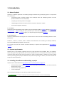
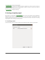
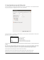
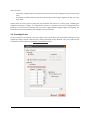
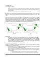
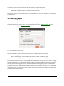
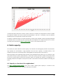
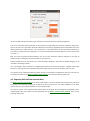
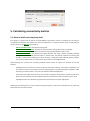
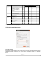
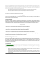
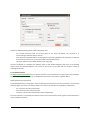
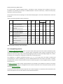
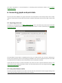
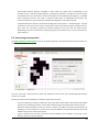
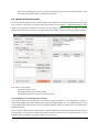
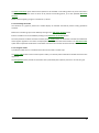
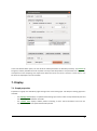
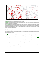
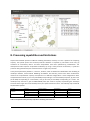
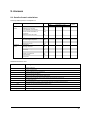
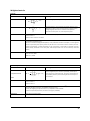
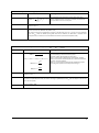
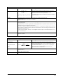
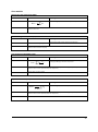
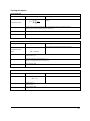
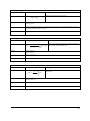
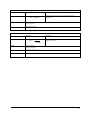
User Manual 2 Summary 1. Introduction .................................................................................................................. 4 1.1. About Graphab .................................................................................................................. 4 1.2. System requirements ......................................................................................................... 4 1.3. Installing the software and launching a project ................................................................... 4 2. Starting a Graphab project ............................................................................................ 5 2.1. Identifying a project ........................................................................................................... 5 2.2. Importing landscape maps and defining nodes.................................................................... 6 2.3. Creating link sets ................................................................................................................ 7 3. Creating graphs ............................................................................................................ 9 4. Patch capacity............................................................................................................. 10 4.1. Capacity as a function of the neighborhood ...................................................................... 10 4.2. Capacity defined from external data ................................................................................. 11 5. Calculating connectivity metrics .................................................................................. 12 5.1. Metrics family and computing level .................................................................................. 12 5.2. Parameters of weighted metrics ....................................................................................... 13 5.3. Calculating batch metrics ................................................................................................. 14 5.4. Interpolating metrics ........................................................................................................ 16 6. Connecting graphs and point data ............................................................................... 17 6.1. Importing points sets ....................................................................................................... 17 6.2. Inter-point distance matrix ............................................................................................... 17 6.3. Generating random points................................................................................................ 18 6.4. Species distribution model ............................................................................................... 19 7. Display ........................................................................................................................ 21 7.1. Graph properties.............................................................................................................. 21 7.2. Object properties ............................................................................................................. 22 8. Processing capabilities and limitations ........................................................................ 23 9. Annexes ...................................................................................................................... 25 9.1. Details of metric calculations ............................................................................................ 25 9.2. References ....................................................................................................................... 33 3 1. Introduction 1.1. About Graphab Graphab is a software application for modeling ecological networks using landscape graphs. It is composed of four modules for: - constructing graphs, including loading initial landscape data and identifying patches and links (Euclidean distances or least-cost paths) - computing connectivity metrics from graphs - integrating graph-based connectivity metrics into species distribution models - visual and cartographic interfacing 1.1.1. Authors Graphab has been developed by Gilles Vuidel and Jean-Christophe Foltête at ThéMA laboratory (University of Franche-Comté – CNRS). Funding has been provided by the French Ministry of Ecology, Energy, Sustainable Development and the Sea (ITTECOP Program). The Graphab logo was designed by Gachwell. 1.1.2. Terms of use Graphab is distributed free-of-charge for non-commercial use. Users must cite the following reference in their publications: Foltête J.C., Clauzel C., Vuidel G., 2012. A software tool dedicated to the modelling of landscape networks, Environmental Modelling & Software, 38: 316-327. For any other use, the prior consent of Théma laboratory is required. Send applications to [email protected]. 1.2. System requirements Graphab runs on any computer supporting Java 1.6 or later (PC under Linux, Windows, Mac, etc.). However, when dealing with very large datasets, the amount of RAM memory in the computer will limit the maximum number of nodes and links that can be processed in a single run with Graphab. In addition, for some complex metrics, processing power (CPU) will determine the speed of computing. For details, see section 8 below and the journal article cited above. 1.3. Installing the software and launching a project Graphab can be downloaded from http://thema.univ-fcomte.fr/productions/graphab. Download and install Java 1.6+ - java.com. If you have a 64-bit operating system, it is best to install the 64-bit version of Java. Download and unzip graphab.zip Launch GraphAB.jar After launching GraphAB.jar, the File menu provides access to four sections: - File / New project: to create a new project in which all data and results are saved automatically. 4 - File / Open project: to open an existing project. - File / Preferences: to change certain software parameters: English/French; maximum amount of memory to use; number of processors to use. It is recommended to adjust the amount of memory and number of processors to suit your computer (see section 8). - File / Log window: to display the event log. 2. Starting a Graphab project New projects are created from the File / New project menu. The user must complete a series of windows to identify the project, import a landscape map, and create a link set. Each project is associated with a single landscape map but may contain several link sets. After the start phase, the project is the medium for creating multiple graphs and for computing connectivity metrics. 2.1. Identifying a project In the first window, the user must enter a project name and specify the folder in which it is to be created. 5 2.2. Importing landscape maps and defining nodes The second window is for importing the landscape map. It must be a raster file (*.tif, *.rst) in which the value of each pixel corresponds to a category (land cover or other classification). If the raster format is *.tif without a Geotiff extension, the file must be associated with a world file for geolocation (*.tfw) structured as follows: Example 10 0 0 -10 821755 2342995 Pixel size in the X-direction Rotation about X-axis Rotation about Y-axis Pixel size in the Y-direction X coordinate of the center of the upper-left pixel Y coordinate of the center of the upper-left pixel If the raster format is *.rst, the file must be associated with a georeferencing file (*.rdc) generated by Idrisi software. The units of the image coordinate system must be meters. If not, the areal and distance units will be incorrect. The image can be reprojected in a metric projection (UTM, Lambert93) using GIS software. No data: pixel value representing the absence of data in the raster file. Habitat patch code: pixel value assigned to the habitat category used to define habitat patches. Minimum patch area: minimum area in hectares for a habitat patch to become a graph node. 6 Patch connexity: 4-connexity: a habitat patch consists of the central pixel with its four neighbors if they are of the same value; 8-connexity: a habitat patch consists of the central pixel with its eight neighbors if they are of the same value. Simplify patch for planar graph: checking the box accelerates the creation of a planar graph, simplifying the polygonal boundaries of patches. This simplification process is not deterministic and so creating two planar graphs for one and the same landscape map may result in slightly different polygon edges. Consequently, this box should not to be checked when planar graphs are to be compared. 2.3. Creating link sets The third window is for creating a link set for which several parameters must be selected: topology and link weighting. Creating a link set is the final step in starting a Graphab project. However, users may create new link sets within the same project via the Graphs / Create link set menu. 7 2.3.1. Link topology Two topologies are available: - planar: only links that form a minimal planar graph are considered. This topology is set up through Voronoi polygons around each habitat patch. These polygons are defined from the edges of patches in Euclidean distance. - complete: all the links between patches are potentially taken into account. Max distance: this option specifies a threshold distance for the complete topology. Links that exceed this distance are no longer created. This limits the number of links created and so accelerates the creation of the link set. Ignore links crossing patch: this default option means that a link between two patches (A and C in the figure below) which crosses an intermediate patch (B) is not created. It is recommended for calculating the betweenness centrality metric (BC) to take into account how often a patch lies on the shortest path between all pairs of patches in the graph. If the option is unchecked, a link is created between two patches (A and C) crossing an intermediate patch, representing the complete true distance between A and C. Save real path: checked box: links are saved as paths representing the actual route of the link between two patches. unchecked box: links are saved in topological form only. In this case, display of links with the realistic view is unavailable. This is recommended for graphs with very many links (e.g. a non-thresholded complete graph) so as to limit the use of memory. Unless paths are saved, intra-patch distances cannot be included in the computation of metrics. 2.3.2. Distance (or link impedance) Distances are calculated from edge to edge between patches. Two main types of distance are available: Euclidean distances and least-cost distances. Euclidean distance: links are defined in Euclidean distances (distance as the crow flies between patches), meaning the matrix is considered to be uniform. Least-cost distance: links are defined in cost distances. Matrix heterogeneity is taken into account by assigning a resistance value (friction) to each landscape category. The user can activate this option in either of two ways: 1) either by specifying different costs for the landscape map categories in the table, 2) or from an external raster file (*.tif or *.rst) in which each pixel has a resistance value. 8 The use of least-cost distance provides two types of impedance using the same paths: cumulative cost: impedance is equal to the sum of the costs of all the pixels along the path, path length: impedance is equal to the metric length of the path. For each link created, its metric distance and its cost-unit distance are saved and available in “link properties” (see section 6.2). 3. Creating graphs A Graphab project may entail the creation of several graphs. Each graph is created from a given link set: either the link set defined in the initial project, or a new link set defined from the Graph / Create link set menu. Graphs are created from the Graph / Create graph menu. First, the new graph must be named. The user must select one of the link sets created in step 2.2. and then select the type of graph: Thresholded graph: the selected links are less than or equal to the selected threshold distance. Non-thresholded graph: all links between patches are validated, regardless of length. Minimum spanning tree: graph connecting all the patches in which the total weight of links is minimal. For a thresholded graph, the unit of the threshold distance depends on the type of distance used in creating the link set. If the link set is created using Euclidean distances, the threshold distance of the graph is in meters. If the link set is created using cost distances, the threshold distance of the graph is given as a cumulative cost. An approximation of the distance metric (DistM) expressed as a cumulative cost (Dist) can be obtained by displaying the scatter plot of the link set (see section 6.2) and using the regression line [Dist = intercept + slope × DistM] to perform the conversion. 9 “Include intra-patch distances for metrics” option: if the box is checked, the computation of metrics includes the distances between and across patches (recommended). If the box is unchecked, only the distances between (but not across) patches are taken into account. To perform a multiscale analysis, it is often necessary to create a series of graphs in which increasing thresholds are defined. Users can create this series manually. But if the objective is to analyze the behavior of a metric according to the threshold, the Metrics / Batch graphs menu can be used (see section 5.3). 4. Patch capacity The capacity of a patch reflects its intrinsic quality as an indicator of its demographic potential. A patch with a high capacity can accommodate a large population and vice versa. Capacity is included directly in the calculation of some area connectivity metrics and weighted connectivity metrics (see section 5). When the project is first created the patch capacity is equal by default to the patch area in m². However, users may replace area by any other quality indicator. In some cases, species presence is related not to patch size but to the area of other types of land cover around the patch. For example, the presence of amphibians in a breeding pond does not depend on the pond size but on the amount of terrestrial habitat surrounding the pond. 4.1. Capacity as a function of the neighborhood The Data / Calculate patch capacity menu can be used to define patch capacity as a function of the neighborhood composition and to calculate it directly from Graphab. 10 Users must define three parameters: type of distance, maximum distance, landscape categories. Cost: This is the spatial metric (Euclidean or cost distance) corresponding to one link set available in the project. The use of costs in this procedure amounts to defining an anisotropic neighborhood around patches which may differ greatly from a buffer function. For consistency, it is recommended to use the same type of distance as was used in creating the links of the graph. For a link set created with Euclidean distance, the user must select “all costs = 1”. Max cost: Like the graph threshold distance, the unit of this maximum distance depends on the type of distance used in creating the link set (Euclidean or cost distance). Codes included: the user may select one or more landscape categories, other than the habitat category, to be included in calculating capacity. The “cost weight” option introduces a weighting with distance to the patch through a negative exponential function. In this way, the areas selected have greater weight if they are close to the patch and vice versa. The capacity values calculated replace the patch area for all subsequent computations. But users can return to the initial parameter via the Data / Calculate patch capacity menu and by selecting “patch area”. 4.2. Capacity defined from external data The Data / Import patch capacity menu allows a data table (*.csv) to be imported describing all the patches of the project and containing capacity values defined in advance by the user. The patch identifiers in the table must be the same as the patch identifiers in the Graphab project. The capacity values in the imported table replace patch area values for all subsequent computations after importing. But users can restore the initial parameter via the Data / Calculate patch capacity menu and by selecting “patch area”. 11 5. Calculating connectivity metrics 5.1. Metrics family and computing level Each graph in a project can be used to compute different connectivity metrics. The details of how they are computed and references are listed in the Annex. Computations are made at several levels corresponding to major sections in the Metrics menu (table 1): - Metrics /Global metrics: describe the entire graph. Metrics /Component metrics: describe connectivity within each component (or sub-graph). Metrics /Local metrics: describe the connectivity of each graph element (node or link). Metrics /Delta metrics: also describe each graph element, but using a specific computing method. Using the removal method (remove nodes or remove links), the relative importance of each graph element is assessed by computing the rate of variation in the global metric induced by each removal. The result of a delta-metric is at a local level but by reference to the global level. After selecting one of these four computing methods, three families of metrics are available in the new window: - weighted metrics are based on criteria of distance and patch capacity. They have to adjusted to suit the reference species. These metrics involve computing paths in a graph via Dijkstra's algorithm. After selecting one of these metrics, the user must specify the desired adjustment. - area metrics are based primarily on the area criterion. If capacity corresponds to a criterion other than patch area, these metrics can be computed and they are expressed in the unit of the criterion used. - topological metrics are derived from graph theory and they do not require adjustment. Whichever the selected level, the user must first specify the graph on which the calculation will be made and then select the connectivity metric. 12 Family Weighted metrics Area metrics Topological metrics Connectivity metrics Flux Probability of connectivity Flow Probability of connectivity Fractions of delta Probability of connectivity Betweenness centrality index Integral index of connectivity Mean size of the components Size of the largest component Class coincidence probability Expected cluster size Node Degree Clustering coefficient Closeness centrality Eccentricity Connectivity correlation Number of components Graph diameter Harary Index Node Degree Code F PC FPC dPC BC IIC MSC SLC CCP ECS Dg CC CCe Ec CCor Cut NC GD H Global × × Computing level Component Local × × × × Delta metrics × × × × × × × × × × × × × × × × × × × × × × × Table 1. Connectivity metrics and computing level 5.2. Parameters of weighted metrics 5.2.1. Alpha parameter Several metrics include a weighting in their calculation which converts the distance between patches into the probability of movement. These metrics are F, PC, FPC, and BC. The weighting is based on an exponential function: 13 where p is the probability of movement between two patches, d the distance between these patches, and α a parameter defining the rate of decline in probability as distance increases. As it is not easy to determine the value of the α parameter, Graphab calculates it from the other two parameters. Users must specify the distance corresponding to a certain value of probability, e.g.: - the maximum dispersal distance of species corresponding to a small value of p (0.05 or 0.01). the average dispersal distance of species corresponding to a median value of p (0.5). The value of α is automatically obtained from the formula: ( )⁄ In the case of a thresholded graph, it is assumed that the distance d used in the setting is consistent with the distance used for the graph thresholding. 5.2.2. Beta parameter The metrics F, PC, FPC, and BC are controlled by the β parameter. This parameter is the exponent applied to patch capacity. It adjusts the relative balance between the weight of distances and the weight of patch capacity in the weighting of metrics. Taking the example of the metric F in local computation, whose generic form is: ∑ - a value of means that the patch capacity plays no part in the weighting. - a value of means that the patch capacity acts linearly in the weighting. - a value of means that the patch capacity is squared in the weighting. - a value of means that the square root of the patch capacity features in the weighting. - a value of means that the patch capacity acts in an inversely proportional way in the weighting. In addition to these few examples, any weighting values are possible. 5.3. Calculating batch metrics Every metric compatible with the global level can be calculated following the variation of the scale of distances. This variation may concern either graph thresholding (5.3.1.), or metric adjustment (5.3.2.). The type of distance used for thresholding depends on the type of distance used in creating the link set (Euclidean, leastcost distance, or least-cost path). 5.3.1. Batch graph The Metrics / Batch graph menu allows a series of thresholded graphs to be created from a given link set and a metric to be calculated for each graph at global level. The thresholds of successive graphs are increasingly defined in either of two ways: - distance: a fixed increment of distance is defined between successive graphs. The metric values are therefore calculated in regular intervals of threshold distance. number of links: a fixed number of links is defined between successive graphs. This number of links is automatically converted into distance used to threshold the graph. These threshold distances may be unevenly spread. 14 Graphs are defined following three criteria selected by users: - min: smallest threshold used for the first graph in the series. By default, this minimum is 0, corresponding to the total absence of links. max: maximum threshold used for the final graph in the series. By default, this maximum corresponds to the maximum distance or to the link number of the selected link set. increment: distance value added between each new graph. Once the calculation is completed, the software opens a new window displaying the curve of the selected metric versus the threshold distance. The values of this curve can be saved with the “Export” button by selecting text format. 5.3.2. Batch parameter The Metrics / Batch parameter menu is used to calculate a series of metrics from a given graph. This procedure applies to the weighted metrics only. It is divided into two entries: local metrics or global metrics. Batch parameter for local metrics A local weighted metric is calculated in series according to the variation of one of its parameters. The user must select the graph, the metric, and the parameter to be varied. The variation of computation is defined by: - min: minimum value of the parameter, max: maximum value of the parameter, increment: interval value between two metric computations. Once the calculation is completed, the patches (and in some cases the links) of the graph are characterized by a series of additional metrics. 15 Batch parameter for global metrics For a given graph, a global weighted metric is calculated in series according to the variation of one of its parameters. As previously, this variation is defined between a minimum value (min), a maximum value (max), and with an interval (increment). The procedure ends with the opening of a new window displaying the curve of the selected metric versus the parameter. Table 2 summarizes possible metrics calculations. Topological metrics Area metrics Weighted metrics Family Connectivity metrics Flux Probability of connectivity Flow Probability of connectivity Fractions of delta Probability of connectivity Betweenness centrality index Integral index of connectivity Mean size of the components Size of the largest component Class coincidence probability Expected cluster size Node Degree Clustering coefficient Closeness centrality Eccentricity Connectivity correlation Number of components Graph diameter Harary Index Code Patch capacity Intrapatch distance Parameters F PC FPC dPC × × × × × × × × × × × × × × × × BC IIC MSC SLC CCP ECS Dg CC CCe Ec CCor NC GD H × × × × × × × × × α β Batch graph Batch parameter × × × × × × × × × × x x × × × × Table 2. Possible connectivity metrics calculations 5.4. Interpolating metrics The Analysis / Metric interpolation menu is used to create raster layers from local metrics calculated at patch level. This transformation is based on a specific spatial interpolation which assigns connectivity values of patches to each cell of a grid, using a decreasing weighting function from the patch edge (weight of 1). Overall, the farther cells are away from the graph, the lower their connectivity values. The weighting is a negative exponential function as for which the user selects a distance (d) corresponding to a certain probability (p) and the software deduces the value of the α parameter. In theory, this adjustment must be consistent with the choice of reference graph or of any weighted metrics, using the same value of d. The Multi connection option allows several patches to be included in the calculation of metrics at the point level. The calculation is based on a weighted mean of values of all patches in the vicinity of the points, up to the specified Maximum distance. The distance used in these calculations depends on the reference graph. If it is based on least-cost distance, the spatial interpolation uses the same distance and not Euclidean distance. 16 The metric interpolation is used automatically in calculating species distribution models; see 6.3. Species distribution model. 6. Connecting graphs and point data The main part of the software is for graph construction and computation of connectivity metrics. But it is often useful to connect these elements with external data. Graphab allows graph data to interact with a points data set. 6.1. Importing points sets Point data can be imported via the Data / Import point set menu. These data may contain several attributes but only binary attributes (presence/absence) are taken into account in certain procedures (see 6.3. Species distribution model). The imported file may be either in shapefile format (*.shp), or in table format (*.csv). For files in table format, the user must specify the columns corresponding to identifiers and to the XY coordinates of points in the table. The attributes to be considered must be selected from the list of attributes available. If point data do not contain an absence attribute, they cannot be used in species distribution models. If the user wants to set up a species distribution model, a set of pseudo-absence points can be generated by the Data / Generate random point menu. 6.2. Inter-point distance matrix Point data imported to Graphab can be used to calculate the inter-point distance matrix by right-clicking on the name of the point data. Several types of distance are available: 17 - Raster-based distance: distance calculated in raster mode for a given link set. Depending on the selected link set, it may be Euclidean distance, cumulative cost distance, or length of a least-cost path. In the latter two cases, calculation includes costs assigned to the landscape map categories, as defined when creating the link set. The result is a distance matrix which is independent of the graph; this matrix corresponds to the calculation provided by the Geographic information Systems. - Graph-based distance: distance calculated according the shortest path in a reference graph. The type of distance is the same as that used in creating the link set of the reference graph. At both ends of a given path, the calculation includes the distance between each point and the nearest patch. Depending on the choice made when creating the graph, the calculation may or may not include intrapatch distances. 6.3. Generating random points The Data / Generate random points menu can be used to generate a set of pseudo-absence points based on a set of presence points. The user must load a file of presence points and specify the name of the set of presence/pseudo-absence points to be created. Several parameters must be defined to randomly sample absence points: - - Cell size of the grid (in meters) to define the size of cells from which absence points will be potentially sampled. The “update grid” button can be used to display the grid according to the selected cell size. Minimum distance between points: this function reduces the effects of spatial autocorrelation by specifying a minimum distance in meters to be observed between the generated absence points and between these points and presence points. Type of distance: the unit of the minimum distance between points depends on the type of the distance used in the link set selected. 18 - Keep only one existing point by cell: this option (checked box) retains only one presence point in each cell thereby reducing the effects of spatial autocorrelation. 6.4. Species distribution model If a set of presence/absence points has been defined, the software can use the connectivity metrics calculated from a graph as predictors in a species distribution model from the Analysis / Species distribution model menu. Such modeling is possible even if points are not located in habitat patches, by means of a spatial extrapolation of the values of metrics. The logistic regression model is a based on minimizing the AIC criterion. First, the user must specify: the set of point data to use, the target variable in the predictive model, the reference graph for the use of connectivity metrics. 6.4.1. Weighting for extrapolating metrics to points The values of metrics are calculated for any point by a spatial interpolation. This interpolation is based on values being weighted by a decreasing function from patch edges (weight of 1). The weight decreases as the same negative exponential function as the one used for weighted metrics (see section 5.2.1), the adjustment is therefore identical. The user selects a distance (d) corresponding to a certain probability (p) and the software deduces the value of the α parameter. In principle, this adjustment must be consistent with the choice of reference graph or of any weighted metrics included in the model, using the same value of d. 19 The Multi connection option allows several patches to be included in calculating metrics at points. Calculation is based on the weighted mean of values of all patches surrounding points, up to the specified Maximum distance. Details of this weighting are given in Foltete et al., 2012a. 6.4.2. Estimating the model The selection of a graph to perform the model displays all available connectivity metrics among predictive variables. Metrics from another graph can be added by clicking on the Add patch variable button. External variables can also be added by clicking on the Add external variable button. Once the predictor variables have been selected, the Fit model button can be used to calculate the coefficients of the logistic regression. The results are displayed on the right-hand side of the window. The Find best model option tests all possible combinations of variables and selects the one that minimizes the AIC criterion. 6.4.3. Using the model A predictive model which is considered to be valid can be used in several ways. The Export table button can be used to export a table (*.csv format) with all statistical variables involved in the regression. The Extrapolate button provides an estimation of the probability of the species presence in all cells of a grid. 20 In the new window which opens, the user finds the model parameters as described previously. The cell size of the grid (in meters) indicates the level of spatial accuracy of the extrapolation. This parameter has a significant consequence on the computing time required to obtain the result. The result is saved as a raster layer in *.tif format and is displayed in the main window. 7. Display 7.1. Graph properties Properties of a graph are available by right-clicking on the name of the graph. Two ways for viewing graphs are available: - The topologic view displays a simplified view of the graph in which nodes are represented by dots and links by straight lines between centroids. The realistic view displays habitat patches according to their actual boundaries and links are represented by least-cost paths between two patches. 21 Topologic view Realistic view The Remove button can be used to remove the graph selected. Properties displays the parameters used in constructing the graph: graph name, graph type with the possible threshold used, and the number of links. The OD Matrix (Origin–Destination Matrix) button creates a table with the distance between each pair of nodes for the given graph. The unit of distance depends on the type of distance used in the graph. The absence of any connection between two nodes is noted NaN. This matrix is saved in the project file in text format named: “graph name- odmatrix.txt ”. 7.2. Object properties The properties of link sets, graph elements (nodes, links, and components), and point data are available by right-clicking on each of them. The Style menu includes the display parameters for objects: color, line width, label, symbol size (for nodes only). Objects can be represented in the same way (single symbol) or according to some attribute. A discretization method can be applied to classify objects according to the values of the selected attribute. By default, the legend of objects is displayed in the table of contents. It can be masked by unchecking the Legend button. The Export menu can be used to export objects to a shapefile (*.shp) or a text file (*.txt). The Statistic menu displays the distribution of the values of one or more attributes: scatter plot: values of two attributes are plotted on a two-dimensional graph, histogram: the bar chart of the values of an attribute is generated. It is also possible to display the values of a given object by selecting it with the white arrow. After selection, the values of attributes are displayed in a new right-hand column named “feature properties”. This column can be closed by clicking on the Properties menu in the top bar. 22 8. Processing capabilities and limitations Graph-based methods provide an efficient modeling framework, but they can raise a question of computing capacity. Two specific points have received particular attention in Graphab: (1) calculation of link sets, (2) calculation of connectivity metrics. All these computations have been optimized by parallelization. This development mode improves computational efficiency by using a multi-processor architecture, a quad-core processor being theoretically four times faster than a single-core processor. In the journal publication [Foltête J.C., Clauzel C., Vuidel G., 2012. A software tool dedicated to the modelling of landscape networks, Environmental Modelling & Software, 38: 316-327], several tests were conducted to measure the computational capacity of Graphab 1.0 in different configurations. Three configurations were compared for these tests: (1) one core (3 Go RAM) corresponding to a current desktop computer, (2) four cores (6 Go RAM) corresponding to a workstation, and (3) 20 cores (15 Go RAM) corresponding to a server. The landscape map used was a grid of 14000*18000 pixels (252 millions of pixels) representing the landscape elements of the region of Franche-Comté (France) at a spatial resolution of 10 m. The landscape map contained 22,634 habitat patches. Topology Complete Planar Distance Euclidean Least-cost Euclidean Least-cost Current desktop 1927s (32 min) 19252s (5h 21 min) 43s 1080s (18 min) Workstation 516s (8 min) 4301s (1h 11 min) 12s 295s (5 min) Server 133s (2 min) 1037s (17 min) 2.6s 82s (1 min) Table 3. Computation times (seconds) required for calculating several link sets 23 In version 1.1, computation times for calculating metrics with intra-patch distances have been optimized. The difference in computation times with or without intra-patch distances is now negligible. The memory used by the software plays an important role. If there is not enough RAM, computation will be slower or may fail (OutOfMemoryError or GC Overhead message). The File/ Preferences / Memory menu can be used to adjust the memory allocated to Graphab. If you have a 32-bit version of Java, Graphab will be limited to about 2 Go (2000 Mo) of memory. If your computer has more than 2 Go of RAM memory, it is highly recommended you install the 64-bit version of Java to use the available memory beyond 2 Go. 24 9. Annexes 9.1. Details of metric calculations Summary table of metrics in Graphab 1.1 Family Weighted metrics Area metrics Topological metrics Connectivity metrics Flux Probability of connectivity Flow Probability of connectivity Fractions of delta Probability of connectivity Betweenness centrality index Integral index of connectivity Mean size of the components Size of the largest component Class coincidence probability Expected cluster size Node Degree Clustering coefficient Closeness centrality Eccentricity Connectivity correlation Number of components Graph diameter Harary Index Code F PC FPC dPC BC IIC MSC SLC CCP ECS Dg CC CCe Ec CCor NC GD H Global × × Computing level Component Local × × × × Delta metrics × × × × × × × × × × × × × × × × × × × × × × Mathematical terms used Terms Meaning Number of patches Number of components Number of patches in the component k All patches close to the patch i Capacity of the patch i (generally the surface area) Capacity of the component k (sum of the capacity of the patches composing k) Area of the study zone Distance between the patches i and j (generally the least-cost distance between them) Probability of movement between the patches i and j Brake on movement distance Exponent to weight more or less capacity 25 Weighted metrics Flux (F) Formula Meaning For the entire graph: sum of potential dispersions from all patches. Global level ∑∑ Local level ∑ For the focal patch i : sum of capacity of patches other than i and weighted according to their minimum distance to the focal patch through the graph. This sum is an indicator of the potential dispersion from the patch i or, conversely to the patch i. Values Values depend on the definition of a. If a represents an area, F expresses an area. Minimum value: 0 Maximum value: Total area of habitat Comment The path used in the graph is the one that maximizes , i.e. the one that minimizes the distance d (or the cost) between the patches i and j. This metric is called Area Weighted Flux (AWF) in some publications. However in Graphab, a is more general because it represents patch capacity, which may be their area or some other criterion chosen by the user. Similarly, the weighting is variable depending on the β parameter. In CS22, AWF is calculated only from patches directly connected to the focal patch, while Graphab takes into account indirectly connected patches. References Urban and Keitt, 2001 Saura and Torné, 2009 Foltête et al., 2012a Probability of Connectivity (PC) Formula Meaning Global level Component level ∑∑ Delta For the entire graph: sum of products of capacity of all pairs of patches weighted by their interaction probability, divided by the square of the area of the study zone. This ratio is the equivalent to the probability that two points randomly placed in the study area are connected. Values Values correspond to a probability. Minimum value: 0 Maximum value: 1 Comment For each pair of patches, the path of the graph used is the one that maximizes minimizes the distance d (or the cost) between the patches i and j. In CS22, the weighting of capacities is set to 1 ; in Graphab it can be modified. If a does not represent patch area, the result is no longer a probability. Reference Saura and Pascual-Hortal, 2007 , i.e. the one that 26 Flow Probability of Connectivity (FPC) Formula Meaning Local level Sum of products of the focal patch capacity with all the other patches, weighted by their interaction probability and divided by the square of the area of the study zone. ∑ Values Minimum value: 0 Maximum value: 1 Comment For each pair of patches, the path of the graph used is one that maximizes , i.e. one that minimizes the distance d (or the cost) between the patches i and j. ∑ This metric is just the local contribution of a patch in the PC index, since . It is the equivalent of the index not divided by the global value of PC. However, the FPC metric is obtained more quickly than because it is not calculated on the basis of patch removal (delta mode). Fractions of delta Probability of Connectivity (dPC, dPCarea, dPCflux, dPCconnector) Formula Meaning ( Delta ) Rate of variation between the value of PC index and the value of PC’ corresponding to the removal of the patch i. The value of dPC is decomposed into three parts: - dPCarea is the variation induced by the area lost after removal; - dPCflux is the variation induced by the loss of interaction between the patch i and other patches; - dPCconnector is the variation induced by the modification of paths connecting other patches and initially routed through i. Values Minimum value: 0 Maximum value: 1 Comment In CS22, the weighting of capacities is set to 1; in Graphab it can be modified. If a does not represent patch area, the result is no longer a probability and dPCarea does not express a loss of area but a loss of capacity. Reference Saura and Rubio, 2010 27 Betweenness Centrality index (BC) Formula Local level Meaning ∑∑ * + Sum of the shortest paths through the focal patch i, each path is weighted by the product of the capacities of the patches connected and of their interaction probability. Pjk represents all the patches crossed by the shortest path between the patches j and k. Values Values depend on the configuration. They correspond to a weight of potential transit. Minimum value: 0 Maximum value: square of the total area of habitat. Comment With an adjustment of α = 0 and β = 0 (uniform weighting of paths), the BC index is the same as that used in other types of graphs. An adjustment of α = 1 and β = 0 gives paths a weight proportional to the product of the capacities of the patches that they connect, whatever their distance. In Foltête et al. (2012a ; 2012b), the BCl index was proposed so as to give greater weight to paths exceeding a given criterion (e.g. dispersal distance). But tests showed that this index was strongly correlated with the weighted BC adjusted with β=0. In Bodin and Saura (2010), the is the weighted BC with d equal to the dispersal distance, as and Reference Bodin and Saura, 2010 Foltête et al., 2012b Integral Index of Connectivity (IIC) Formula Meaning Global level Component level ∑∑ Delta Values Minimum value: 0 Maximum value: 1 Reference Pascual-Hortal and Saura, 2006 For the entire graph: product of patch capacities divided by the number of links between them, the sum is divided by the square of the area of the study zone. IIC is built like the PC index but using the inverse of a topological distance rather than a negative exponential function of the distance based on the link impedance. 28 Area metrics Mean Size of the Components (MSC) Formula Meaning For the entire graph: mean of the component capacities. Global level Values ∑ Minimum value: minimum capacity Maximum value: Size of the Largest Component (SLC) Formula Meaning * Global level Values + For the entire graph: largest capacity of components. Minimum value: minimum capacity Maximum value: maximum capacity Class Coincidence Probability (CCP) Formula Meaning Global level ∑( ∑ ) For the entire graph: probability that two points randomly placed on the graph belong to the same component. Values Minimum value: minimum capacity (as many components as patches and regular capacities) Maximum value: sum of capacities (only one component) Reference Pascual-Hortal and Saura, 2006 Expected Cluster Size (ECS) Formula Meaning For the entire graph: size of a component Global level ∑ ∑ Values Minimum value: minimum capacity (as many components as patches and regular capacities) Maximum value: sum of capacities (only one component) Reference O’Brien et al., 2006 29 Topological metrics Harary Index (H) Formula Global level Meaning ∑∑ Sum of the inverse of the number of links between all pairs of patches. Component level Values Minimum value: minimum capacity (as many components as patches and regular capacities) Maximum value: sum of capacities (only one component) Comment For pairs of patches not connected by a path, we have : Reference Ricotta et al., 2000 Graph Diameter (GD) Formula Meaning Greatest distance between two patches of the graph. Global level Component level Delta Values Minimum value: 0 Maximum value: Comment When the nodes i and j are not related This metric is the global version of the metric Reference Urban and Keitt, 2001 Number of Components (NC) Formula Meaning Number of components of the graph. Global level Values Minimum value: 1 Maximum value : Reference Urban and Keitt, 2001 30 Node Degree (Dg) Formula Meaning Number of the patches close to the patch i Local level | | Values Minimum value: 0 Maximum value: Comment There is an equivalence between the node degree and the number of nearest patches because graphs are not oriented and do not contain any loops. Reference Freeman, 1979 Clustering Coefficient (CC) Formula Meaning Local level | |(| | Values Minimum value: 0 Maximum value: 1 Comment Si | | Reference Ricotta et al., 2000 ) ∑| | Ratio of the number of nodes close to i which are neighbors to each other over the possible total. Closeness Centrality (CCe) Formula Local level Meaning ∑ Values Minimum value: 0 Maximum value: Comment Si Reference Freeman, 1979 Mean distance from the patch i to all other patches of its component k. 31 Eccentricity (Ec) Formula Meaning Maximum distance from the patch i to another patch of its component k. Local level Values Minimum value: 0 Maximum value: Reference Urban and Keitt, 2001 Connectivity correlation (CCor) Formula Meaning Local level | | ∑ Values Minimum value: 0 Maximum value: | | Comment Si | | Reference Minor and Urban, 2008 | | Ratio between the degree of the node i and the degree of its neighboring patches j 32 9.2. References Bodin O., Saura S., 2010. Ranking individual habitat patches as connectivity providers: Integrating network analysis and patch removal experiments. Ecological Modelling 221, 2393–2405. Foltête J.C., Clauzel C., Tournant P., Vuidel G., 2012a, Integrating graph-based connectivity metrics into species distribution models, Landscape Ecology 27, 557-569. Foltête J.C., Clauzel C., Vuidel G., 2012b. A software tool dedicated to the modelling of landscape networks. Environmental Modelling and Software 38, 316-327. O’Brien D., Manseau M., Fall A., Fortin M.J., 2006. Testing the importance of spatial configuration of winter habitat for woodland caribou: An application of graph theory. Biological Conservation 130, 70–83. Minor E.S., Urban D.L., 2008. A graph-theory framework for evaluating landscape connectivity and conservation planning. Conservation Biology 22, 297–307. Pascual-Hortal L., Saura S., 2006. Comparison and development of new graph-based landscape connectivity indices: towards the priorization of habitat patches and corridors for conservation. Landscape Ecology 21, 959–967 Rayfield B., Fortin M.J., Fall A., 2011. Connectivity for conservation: a framework to classify network measures. Ecology 92, 847–858. Ricotta C., Stanisci A., Avena G.C., Blasi C., 2000, Quantifying the network connectivity of landscape mosaics: a graphtheoretical approach, Community Ecology 1(1), 89–94. Saura S., Pascual-Hortal L., 2007. A new habitat availability index to integrate connectivity in landscape conservation planning: Comparison with existing indices and application to a case study. Landscape and Urban Planning 83, 91– 103. Saura S., Torné J., 2009. ConeforSensinode 2.2: A software package for quantifying the importance of habitat patches for landscape connectivity. Environmental Modelling and Software 24, 135–139. Saura S., Rubio L., 2010. A common currency for the different ways in which patches and links can contribute to habitat availability and connectivity in the landscape. Ecography 33, 523–537. Urban D.L., Keitt T.H., 2001. Landscape connectivity: a graph theoretic approach. Ecology 82, 1205–1218. 33