Download ASPRO-VLTI User's Manual - Observation and Data Reduction with

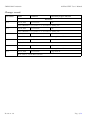
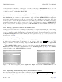
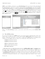
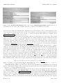
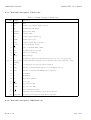
JMMC-MAN-2100-002
Revision 6.0
Date:
02/05/2006
JMMC
ASPRO-VLTI User’s Manual
Authors:
Gaspard Duchˆene <[email protected]> — LAOG/JMMC
Gilles Duvert <[email protected]> — LAOG/JMMC
Daniel Bonneau <[email protected]> — OCA/JMMC
Olivier Chesneau <[email protected]> — OCA/JMMC
Author: Gaspard Duchˆene
Signature:
Institute: LAOG/JMMC
Date: 02/05/2006
Approved by: G´erard Zins
Signature:
Institute: LAOG/JMMC
Date: 02/05/2006
Released by: Gilles Duvert
Signature:
Institute: LAOG/JMMC
Date: 02/05/2006
JMMC-MAN-2100-002
ASPRO-VLTI User’s Manual
Change record
Revision
Date
Authors
Sections/Pages affected
Remarks
1.0
01/03/2005
G. Duchˆene
all
User’s Manual for preparation of observations during P75
2.0
18/03/2005
G. Duchˆene
all
User’s Manual for preparation of observations during P76
3.0
13/09/2005
G. Duchˆene
all
User’s Manual for preparation of observations during P76 and P77
4.0
20/02/2006
G. Duchˆene
25-end
Updated for SearchCal 3.3
5.0
16/03/2006
G. Duchˆene
all
User’s Manual for preparation of observations during P77 and P78
6.0
02/05/2006
G. Duchˆene
Appendix A
New version of SearchCal software
Revision: 6.0
Page 2/30
JMMC-MAN-2100-002
ASPRO-VLTI User’s Manual
Table of contents
1 Introduction
1.1 Object . . . . . . . . . . . . . . . . . . . . . . . . . . . . . . . . . . . . . . . . . . . . . . . . .
1.2 Reference documents . . . . . . . . . . . . . . . . . . . . . . . . . . . . . . . . . . . . . . . . .
1.3 Abbreviations and acronyms . . . . . . . . . . . . . . . . . . . . . . . . . . . . . . . . . . . . .
4
4
4
4
2 Overview
2.1 Brief functional description . . . . . . . . . . . . . . . . . . . . . . . . . . . . . . . . . . . . .
2.2 System requirements . . . . . . . . . . . . . . . . . . . . . . . . . . . . . . . . . . . . . . . . .
5
5
5
3 Using ASPRO-VLTI
3.1 Launching the ASPRO package . . . . . . . . . . . . . . . . . . . . .
3.1.1 The launcher applet . . . . . . . . . . . . . . . . . . . . . . .
3.1.2 Anonymous vs. authenticated login on the ASPRO server . .
3.1.3 Setting a personal account on the ASPRO server . . . . . . .
3.1.4 Starting the ASPRO package . . . . . . . . . . . . . . . . . .
3.1.5 Uploading and downloading files to/from the ASPRO server
3.2 The ASPRO package . . . . . . . . . . . . . . . . . . . . . . . . . . .
3.3 First contact with ASPRO-VLTI . . . . . . . . . . . . . . . . . . .
3.4 EXIT menu . . . . . . . . . . . . . . . . . . . . . . . . . . . . . . .
3.5 OBJECT menu . . . . . . . . . . . . . . . . . . . . . . . . . . . . .
3.5.1 Manual Object Entry . . . . . . . . . . . . . . . . . . . . .
3.5.2 Get CDS Object By Name . . . . . . . . . . . . . . . . .
3.5.3 Calibrator(s) . . . . . . . . . . . . . . . . . . . . . . . . . .
3.6 OBSERVATIONAL SETUP menu . . . . . . . . . . . . . . . . .
3.7 UV PLOTS menu . . . . . . . . . . . . . . . . . . . . . . . . . . . .
3.8 FIT MODEL menu . . . . . . . . . . . . . . . . . . . . . . . . . . .
3.8.1 Fit UV Data . . . . . . . . . . . . . . . . . . . . . . . . . .
3.8.2 Model Parameter Errors Calculator . . . . . . . . . . .
3.9 PLOT menu . . . . . . . . . . . . . . . . . . . . . . . . . . . . . . .
3.10 MISC menu . . . . . . . . . . . . . . . . . . . . . . . . . . . . . . .
3.10.1 Show Current Setup . . . . . . . . . . . . . . . . . . . . .
3.10.2 Plot Current Interferometer Setup . . . . . . . . . . . .
3.10.3 Reset Marker Size . . . . . . . . . . . . . . . . . . . . . . .
3.10.4 Use Big Markers . . . . . . . . . . . . . . . . . . . . . . . .
3.10.5 Exit From Error Loop . . . . . . . . . . . . . . . . . . . .
3.10.6 Ignore Error . . . . . . . . . . . . . . . . . . . . . . . . . .
3.10.7 List UV Table Content . . . . . . . . . . . . . . . . . . . .
A SearchCalibrators Tool
A.1 Goals . . . . . . . . . . . . . . . . . . . . . . . . . . . . . .
A.2 Method . . . . . . . . . . . . . . . . . . . . . . . . . . . . .
A.2.1 N-Band case . . . . . . . . . . . . . . . . . . . . . .
A.2.2 Other Bands . . . . . . . . . . . . . . . . . . . . . .
A.3 Further selection of the calibrators . . . . . . . . . . . . . .
A.4 Results of the SearchCalibrators tool . . . . . . . . . . . . .
A.4.1 Initial selection . . . . . . . . . . . . . . . . . . . . .
A.4.2 Refining the selection . . . . . . . . . . . . . . . . .
A.5 Description of columns in the Search Calibrator result panel
A.5.1 Short list column description, N-Band case . . . . .
A.5.2 Short list column description, JHK-Band case . . . .
Revision: 6.0
.
.
.
.
.
.
.
.
.
.
.
.
.
.
.
.
.
. .
. .
.
.
.
.
.
.
.
.
.
.
.
.
.
.
.
.
.
.
.
.
.
.
.
.
.
.
.
.
.
.
.
.
.
.
.
.
.
.
.
.
.
.
.
.
.
.
.
.
.
.
.
.
.
.
.
.
.
.
.
.
.
.
.
.
.
.
.
.
.
.
.
.
.
.
.
.
.
.
.
.
.
.
.
.
.
.
.
.
.
.
.
.
.
.
.
.
.
.
.
.
.
.
.
.
.
.
.
.
.
.
.
.
.
.
.
.
.
.
.
.
.
.
.
.
.
.
.
.
.
.
.
.
.
.
.
.
.
.
.
.
.
.
.
.
.
.
.
.
.
.
.
.
.
.
.
.
.
.
.
.
.
.
.
.
.
.
.
.
.
.
.
.
.
.
.
.
.
.
.
.
.
.
.
.
.
.
.
.
.
.
.
.
.
.
.
.
.
.
.
.
.
.
.
.
.
.
.
.
.
.
.
.
.
.
.
.
.
.
.
.
.
.
.
.
.
.
.
.
.
.
.
.
.
.
.
.
.
.
.
.
.
.
.
.
.
.
.
.
.
.
.
.
.
.
.
.
.
.
.
.
.
.
.
.
.
.
.
.
.
.
.
.
.
.
.
.
.
.
.
.
.
.
.
.
.
.
.
.
.
.
.
.
.
.
.
.
.
.
.
.
.
.
.
.
.
.
.
.
.
.
.
.
.
.
.
.
.
.
.
.
.
.
.
.
.
.
.
.
.
.
.
.
.
.
.
.
.
.
.
.
.
.
.
.
.
.
.
.
.
.
.
.
.
.
.
.
.
.
.
.
.
.
.
.
.
.
.
.
.
.
.
.
.
.
.
.
.
.
.
.
.
.
.
.
.
.
.
.
.
.
.
.
.
.
.
.
.
.
.
.
.
.
.
.
.
.
.
.
.
.
.
.
.
.
.
.
.
.
.
.
.
.
.
.
.
.
.
.
.
.
.
.
.
.
.
.
.
.
.
.
.
.
.
.
.
.
.
.
.
.
.
.
.
.
.
.
.
.
.
.
.
.
.
.
.
.
.
.
.
.
.
.
.
.
.
.
.
.
.
.
.
.
.
.
.
.
.
.
.
.
.
.
.
.
.
.
.
.
.
.
.
.
.
.
.
.
.
.
.
.
.
.
.
.
.
.
.
.
.
.
.
.
.
.
.
.
.
.
.
.
.
.
.
.
.
.
.
.
.
.
.
.
.
.
.
.
.
.
.
.
.
.
.
.
6
6
6
7
7
7
7
8
9
10
10
10
13
13
15
17
18
18
20
20
20
20
21
21
21
21
21
22
.
.
.
.
.
.
.
.
.
.
.
23
23
23
23
23
24
24
24
25
27
27
28
Page 3/30
JMMC-MAN-2100-002
ASPRO-VLTI User’s Manual
A.5.3 Full table description, N-Band case . . . . . . . . . . . . . . . . . . . . . . . . . . . . . 29
A.5.4 Full table description, JHK-Band case . . . . . . . . . . . . . . . . . . . . . . . . . . . 29
List of Tables
1
2
3
4
5
6
7
List of available analytical models and the parameters that describe them. . . .
Quantities that can be selected to plot the results of the simulated observations.
Magnitude Search Range vs. Flux of Object. . . . . . . . . . . . . . . . . . . . .
Short list column description, N-Band case . . . . . . . . . . . . . . . . . . . . .
Short list column description, JHK Bands case . . . . . . . . . . . . . . . . . . .
Column description, N-Band case . . . . . . . . . . . . . . . . . . . . . . . . . . .
Column description JHK bands case . . . . . . . . . . . . . . . . . . . . . . . . .
.
.
.
.
.
.
.
.
.
.
.
.
.
.
.
.
.
.
.
.
.
.
.
.
.
.
.
.
.
.
.
.
.
.
.
.
.
.
.
.
.
.
.
.
.
.
.
.
.
12
19
23
28
28
29
30
List of Figures
1
2
3
4
5
6
7
8
9
10
11
12
13
14
15
16
17
18
19
20
21
22
23
24
Outline of the usage of ASPRO-VLTI. Users go through each of these four main modules
and obtain some quantitative results indicated below each module. . . . . . . . . . . . . . .
The Application Applet window for anonymous (left) and personal account (right) login
to ASPRO-VLTI. . . . . . . . . . . . . . . . . . . . . . . . . . . . . . . . . . . . . . . . . .
The new tabs appearing in the Application Applet window after ASPRO-VLTI has been
launched. . . . . . . . . . . . . . . . . . . . . . . . . . . . . . . . . . . . . . . . . . . . . . . .
The File Exchange windows to upload and download files from a personal ASPRO-VLTI
account. . . . . . . . . . . . . . . . . . . . . . . . . . . . . . . . . . . . . . . . . . . . . . . .
The two GUI windows that are automatically opened upon launching the ASPRO package:
the start-up control window (top) and the graphical window (bottom left). . . . . . . . . . .
The appearance of the main control window GUI once the user has selected a version ASPROVLTI. . . . . . . . . . . . . . . . . . . . . . . . . . . . . . . . . . . . . . . . . . . . . . . . . .
The All About My Source panel opened by the Manual Object Entry menu in the case
of a parametric model of the source (default, left) and of a user-provided FITS model (right).
The Get Source Coordinates panel opened by the Get CDS Object By Name menu
(left) and the resulting All About My Source panel (right). . . . . . . . . . . . . . . . . .
The Search Calibrators panel opened by the Calibrator(s) menu. . . . . . . . . . . . . .
The window presenting the results of the Search Calibrators tool. . . . . . . . . . . . . . . .
The default Setup For Observation panel (left) and the resulting UV coverage plot for a
E Gauss model (right). . . . . . . . . . . . . . . . . . . . . . . . . . . . . . . . . . . . . . .
The Observability panel (left) and the resulting time coverage plot (right). . . . . . . . . .
The Setup For Observation panel with the Less Used Observing Constraints (left)
and Additional Plotting Constraints (right) sub-panels. . . . . . . . . . . . . . . . . . .
The Interferometric Observables Explorer panel (left) and a visibility plot (right). . . .
UV fit control panel (left) and result windows (right) for the Fit UV Data procedure for
two different models fitted to the same synthetic dataset. . . . . . . . . . . . . . . . . . . . .
Current setup panel (left) and UV table listing (right) obtained from the MISC menu. . . .
Result Panel . . . . . . . . . . . . . . . . . . . . . . . . . . . . . . . . . . . . . . . . . . . . .
Refining the selection . . . . . . . . . . . . . . . . . . . . . . . . . . . . . . . . . . . . . . . . .
Field Selection Tool . . . . . . . . . . . . . . . . . . . . . . . . . . . . . . . . . . . . . . . . .
Maximum magnitude difference Selection Tool . . . . . . . . . . . . . . . . . . . . . . . . . .
Spectral Types Selection Tool . . . . . . . . . . . . . . . . . . . . . . . . . . . . . . . . . . . .
Luminosity class Selection Tool . . . . . . . . . . . . . . . . . . . . . . . . . . . . . . . . . . .
Maximal expected accuracy Selection Tool . . . . . . . . . . . . . . . . . . . . . . . . . . . . .
Variability Selection Tool . . . . . . . . . . . . . . . . . . . . . . . . . . . . . . . . . . . . . .
Revision: 6.0
5
6
7
8
9
9
11
13
14
14
16
16
17
18
20
21
24
25
26
26
26
27
27
27
Page 4/30
JMMC-MAN-2100-002
25
ASPRO-VLTI User’s Manual
Multiplicity Selection Tool . . . . . . . . . . . . . . . . . . . . . . . . . . . . . . . . . . . . . . 27
Revision: 6.0
Page 5/30
JMMC-MAN-2100-002
1
ASPRO-VLTI User’s Manual
Introduction
1.1
Object
This document describes the usage of ASPRO-VLTI, a software derived from the JMMC general software for preparing interferometric observations, ASPRO. ASPRO-VLTI allows users to simulate VLTI
observations with the setups offered by ESO for Period 77 and 78.
1.2
Reference documents
[1] JMMC-MAN-2100-001, Revision 2.0, ASPRO User’s Manual
1.3
Abbreviations and acronyms
AMBER
Astronomical Multi Beam Recombiner
ASPRO
Astronomical Software to PrepaRe Observations
AT
Auxiliary Telescope
CDS
Centre de Donn´ees astronomiques de Strasbourg
CHARA
Center for High Angular Resolution Astronomy
COAST
Cambridge Optical Aperture Synthesis Telescope
DFT
Discrete Fourier Transform
ESO
European Southern Observatory
ETC
Exposure Time Calculator
FAQ
Frequently Asked Questions
FITS
Flexible Image Transport System
FWHM
Full Width at Half-Maximum
GI2T
Grand Interf´erom`etre `a 2 T´elescopes
GILDAS
Grenoble Image and Line Data Analysis System
GUI
Graphic User Interface
IOTA
Infrared Optical Telescope Array
IRAM
Institut de RadioAstronomie Millim´etrique
JMMC
Jean-Marie Mariotti Center
MIDI
MID-infrared Instrument
PDF
Portable Document Format
PS
PostScript
PTI
Palomar Testbed Interferometer
RMS
Root Mean Square
SIMBAD
Set of Identifications, Measurements and Bibliography for Astronomical Data
UT
Unit Telescope
VLTI
Very Large Telescope Interferometer
XML
eXtensible Markup Language
Revision: 6.0
Page 6/30
JMMC-MAN-2100-002
2
ASPRO-VLTI User’s Manual
Overview
2.1
Brief functional description
ASPRO-VLTI is designed to allow effortless usage by any astronomer; in particular, no detailed knowledge of optical interferometry is required. The only prior information that the user should provide is the
instrument he/she would like to use and the physical properties of his/her target. ASPRO-VLTI provides
tools to determine the optimal VLTI configuration and interferometric calibrators to achieve the user’s astrophysical goals. The optimization is performed through estimating synthetic interferometric observables
(visibilities) as well as through fitting theoretical models on these quantities. The fitting process takes into
account the measurement errors of the interferometric signal based on the instrument’s ETC.
ASPRO-VLTI is organized as a suite of four main successive modules (see Fig. 1), which are briefly
presented below and described in more details later in Sect. 3. The four modules are:
– OBJECT: to define the target properties (name, coordinates, photometry and model of its geometry);
– OBSERVATIONAL SETUP: to define the VLTI configuration to be used in the observations; this
includes defining both the telescope array and the instrumental setup;
– UV PLOTS: to calculate and plot interferometric observables and their associated uncertainties;
– FIT MODEL: to fit parametric models to the synthetic interferometric signal that are created by
the UV PLOTS module.
Figure 1: Outline of the usage of ASPRO-VLTI. Users go through each of these four main modules and
obtain some quantitative results indicated below each module.
The UV coverage of the object with VLTI is provided by the OBSERVATIONAL SETUP module.
With the UV PLOTS module, the user can readily estimate if observing the target in the requested
configuration will yield visibilities that are accurately measurable and that vary significantly as a function
of time, for instance. The FIT MODEL module allows the user to estimate whether the observations
would yield tight constraints on the geometrical model of the source, possibly leading to the exclusion of
some models, for instance. In addition to these outputs, ASPRO-VLTI also provides a tool to search
for adequate interferometric calibrators; the user is provided with a list of objects, along with a number of
relevant properties, from which the most appropriate ones can be selected.
2.2
System requirements
ASPRO-VLTI is run remotely through the JMMC website. It is normally run as a Java2 applet, which
means that the appropriate Java plug-in (version 1.1.2 or higher) must be installed. If it is not installed,
please install the computer-specific plug-in first (see http://java.sun.com).
ASPRO-VLTI can be used in anonymous or authenticated mode. Authenticated mode permits to
exchange files with the server and retrieve previously stored user preferences and files. When launching
ASPRO-VLTI anonymously, the user connects to one of the 16 ASPRO-VLTI visitor accounts available.
If all accounts are already being used, the application will not start and the user must try again later. All
Revision: 6.0
Page 7/30
JMMC-MAN-2100-002
ASPRO-VLTI User’s Manual
connections use one IP port in the range 50000-52500. In case of systematic failure to start the application,
the user must check that he/she is not working in front of a firewall that blocks part of this port range.
An alternative method to start ASPRO-VLTI is to launch it as a Java Webstart application, also
available from the JMMC website. This only requires the installation of Java Runtime Tool Kit on the
user’s computer, also available from http://java.sun.com.
The ASPRO-VLTI GUI has been created by JMMC based on Java and XML technologies. The use of
the GUI should be totally transparent to the user; if necessary, a document describing the basic principles
of the XML-based GUI is available from the JMMC website.
3
Using ASPRO-VLTI
This section describes how to launch the ASPRO package and to use ASPRO-VLTI, which is a part of
this package. If problems occur while running ASPRO-VLTI, check here for possible errors in selecting
options or providing information to the software. Furthermore, right-clicking (<CTRL>-click for Macintosh
users) on a variable/parameter name in any panel brings up a brief explanation of its nature and possible
values. In addition, use the Help buttons available in each ASPRO-VLTI panel. If no solution to a
problem can be found there or in the ASPRO-VLTI FAQ webpage on the JMMC website, please send
an email to the JMMC User Support group ([email protected]) with a detailed
description of the problem (including input parameters and error messages appearing in the LOG window,
if any).
Each of the OBJECT, OBSERVATIONAL SETUP, UV PLOTS and FIT MODEL panels,
which are described below, contains a CLOSE button to dismiss it. However, navigation between modules
of ASPRO-VLTI should normally be performed with the Proceed to ... and Back to... buttons, a
method which ensures that the four main modules of ASPRO-VLTI are used in the appropriate order.
Note ASPRO-VLTI generates several files as commands are executed and uses them in other modules.
The naming convention of these files, which can be retrieved by the user from his/her ASPRO-VLTI
account, is automatic and cannot be modified by the user.
3.1
3.1.1
Launching the ASPRO package
The launcher applet
Figure 2: The Application Applet window for anonymous (left) and personal account (right) login to
ASPRO-VLTI.
To start a new ASPRO-VLTI session, click on the Start the Application Launcher Applet icon/link
in the ASPRO webpage. If the appropriate Java2 applet is installed (see Sect. 2.2), an Application Applet window will appear on the user’s screen (see left part of Fig. 2). Select Help under the ? menu for
Revision: 6.0
Page 8/30
JMMC-MAN-2100-002
ASPRO-VLTI User’s Manual
a basic description of the usage of the applet. Note that, at this stage, ASPRO-VLTI has not yet been
started; the Java applet has only initiated a new “session”, from which it is possible to start the entire suite
of JMMC softwares, including ASPRO-VLTI.
3.1.2
Anonymous vs. authenticated login on the ASPRO server
The user can decide to launch ASPRO-VLTI either anonymously (default option offered by the Application Applet window) or using a pre-defined username. First- or one-time ASPRO-VLTI users can usually
accommodate using the anonymous login option. For frequent ASPRO-VLTI users and/or for repeated
use of some custom input/setup files, the use of a personal account is usually more appropriate. Note that
it is not possible to upload files (such as FITS files representing object models) to the JMMC servers using
anonymous login, nor is it possible to retrieve files created or used during previous use of ASPRO-VLTI.
It is however possible to save any plot generated by ASPRO-VLTI as a PS or PDF file with either type
of login.
3.1.3
Setting a personal account on the ASPRO server
Setting a personal account can be done simply by subscribing to the aspro-users mailing list. After sending
an email to [email protected] (with sub aspro-users in the subject line), the user will
receive a confirmation email containing his/her username and password. These are the entries to provide in
the Application Applet window after checking the Start application using my account informations box
(see right part of Fig. 2).
3.1.4
Starting the ASPRO package
To start the entire ASPRO package, which includes ASPRO-VLTI, either anonymously or after logging
in with a valid username/password combination (do not forget to click on the Login button once after
filling the username and password fields), simply select ASPRO in the Start menu of the Application
Applet.
When ASPRO-VLTI is launched, one or two new tab(s) appear in the Application Applet window:
ASPRO and, if the user has used an authenticated login, File Management (see Fig. 3). The ASPRO
tab should indicate that ASPRO-VLTI is now running.
Figure 3: The new tabs appearing in the Application Applet window after ASPRO-VLTI has been
launched.
3.1.5
Uploading and downloading files to/from the ASPRO server
If the user has started the application with an authenticated login, the Open File Exchange Panel button
in the File Management tab allows him/her to upload/download files from his/her personal ASPRORevision: 6.0
Page 9/30
JMMC-MAN-2100-002
ASPRO-VLTI User’s Manual
VLTI account. Clicking on this button opens a File Exchange window (see left part of Fig. 4) that lists all
files currently present on the user’s account (it is empty when the account has just been created). Checking
the Enable File Management box opens a second sub-panel in the File Exchange window (see right part
of Fig. 4) that lists and allows to browse the files and directories present on the user’s personal computer.
To upload a file on the JMMC servers, highlight the file in the Local File System sub-panel and click
on the < button; the file should appear in the Remote File System sub-panel. Reversely, to download
a file from the JMMC servers, select the file and click on the > button after selecting the appropriate
download directory. Click on the Cancel button in the Remote File System sub-panel to dismiss the
File exchange window.
Figure 4: The File Exchange windows to upload and download files from a personal ASPRO-VLTI
account.
3.2
The ASPRO package
Once the user has launched the ASPRO package, he is presented with two GUI windows (see Fig. 5): the
graphic window, in which plots will be presented when running ASPRO-VLTI, and the start-up control
window. At this stage, the start-up control window contains only a Choose menu, from which the user
actually selects the JMMC software he wants to use for this session. The possible choices are:
– AMBER 3T Period 78 and 77
– AMBER 2T Period 78 and 77
– MIDI on UTs Period 78 and 77
– MIDI on ATs Period 78 and 77
– Full ASPRO Interface
The first four choices represent the specific versions of ASPRO-VLTI available for preparing observations for Period 77 or 78. They allow the user to choose the instrument (MIDI or AMBER) and the
type (UTs or ATs for MIDI; AMBER is only offered with UTs for Periods 77 and 78) or number (2 or 3
for AMBER; MIDI only allows 2-telescope interferometry) of telescopes. Note that the technical details of
both AMBER and MIDI instruments are unchanged between Period 77 and 78. The appearance and usage
of ASPRO-VLTI is essentially the same for all versions, with only minor details varying from one to the
other (such as the instrument sensitivities or the observing wavelength). In the remainder of this document,
Revision: 6.0
Page 10/30
JMMC-MAN-2100-002
ASPRO-VLTI User’s Manual
Figure 5: The two GUI windows that are automatically opened upon launching the ASPRO package: the
start-up control window (top) and the graphical window (bottom left).
we describe the usage of MIDI on UTs Period 78 and 77, and only explicitly discuss the specificities of
other versions when needed.
The Full ASPRO Interface choices starts up the wider-scope ASPRO software, which allows simulations of observations with other interferometers (CHARA, COAST, GI2T, IOTA, IRAM’s Plateau de Bure,
PTI) as well as configuration of VLTI with MIDI and AMBER that are not available for Period 78 and with
future VLTI instruments allowing observations with 4- and 8-telescope arrays. This version of the software
is not described here; a specific Users’ Manual is available from JMMC.
3.3
First contact with ASPRO-VLTI
Once a specific version of ASPRO-VLTI has been selected, the main control window offers seven menus
(see Fig. 6). The EXIT menu allows to quit ASPRO-VLTI. The OBJECT, OBSERVATIONAL
SETUP, UV PLOTS and FIT MODEL menus allow the user to enter the four main modules constituting
ASPRO-VLTI (see Fig. 1). The PLOT and MISC modules offer several helpful commands that can be
used at any time while running ASPRO-VLTI. All menus are described in more detail in the remainder
of this document.
Figure 6: The appearance of the main control window GUI once the user has selected a version ASPROVLTI.
In addition to these main menus, the main control window contains an Help button and a button
to open the LOG window in which ASPRO-VLTI prints out messages as it executes commands. The
content of the LOG window can be useful while troubleshooting. To the left of these two buttons is a whitebackground window in which ASPRO-VLTI provides short statements about its status while running
commands; it is usually empty when the software is idle. Finally, to the left of this window is a roundish
icon whose color indicates ASPRO-VLTI status: when it is green, the software is up and running and
waiting for commands from the user; when it is orange, it is executing a command; when it is red, the
software has run into an error and stopped. Commands can only be executed when this icon is green. If it
is orange, wait for the command to be completed. If it is red (or stuck on orange for at least a couple of
minutes), try using (a few times if necessary) Exit From Error Loop in the MISC menu (see Sect. 3.10.5).
Revision: 6.0
Page 11/30
JMMC-MAN-2100-002
ASPRO-VLTI User’s Manual
If this is not enough to restore a normal running state for ASPRO-VLTI, then there has been a severe
crash; it is then recommended to quit ASPRO-VLTI and restart if from scratch. If the same problem
occurs repeatedly, checking the content of the LOG window may provide an indication of the nature of the
problem.
The buttons located in the top left corner of the graphical window represent the following, from left to
right:
– Refresh Plot redraws the last plot requested in case it did not show up automatically or if the
displays contains only a red square crossed by two thin white diagonals;
– Zoom In increases the zoom factor and provides scrolling bars to move around in the plot;
– Zoom Out decreases the zoom factor;
– Toggle Scrolling Bars On and Off adjusts the window size to the current zoom while removing
the scrolling bars;
– the Anti-Aliasing option can be used for improving the quality of the graphical display on your
computer screen.
3.4
EXIT menu
The only command under the EXIT menu, Exit From ASPRO-MIDI UT quits the ASPRO-VLTI
software after confirmation in a pop-up window. After the software is shut down (the GUI windows are
dismissed), the Application Applet window remains in the user’s screen, but the ASPRO tab has now
disappeared. The configuration of the applet window is identical to its status after the user has first started
the applet (see Fig. 2); in particular, if the user had logged in with his/her personal account information,
he/she has been automatically logged out. Clicking on the EXIT button terminates the current ASPROVLTI session.
3.5
OBJECT menu
This menu brings up the first main module constituting ASPRO-VLTI: the object definition module.
Here, the user must provide all properties that define the interferometric target: its name, coordinates,
brightness and a model of its geometry. The coordinates of the object can be entered by hand (see Sect. 3.5.1)
or retrieved from the CDS database (see Sect. 3.5.2). Also, ASPRO-VLTI provides a tool to find the
most appropriate calibrators for a given scientific target, taking into account the required accuracy on the
visibilities (see Sect. 3.5.3).
3.5.1
Manual Object Entry
Selecting Manual Object Entry under the OBJECT menu brings up the All About My Source panel
illustrated in the left part of Fig. 7.
In the upper half of the panel, the user must provide the target name (Source Name, with no more than
24 characters and no embedded <space>; use <underscore> instead), its J2000 coordinates (RA 2000 and
DEC 2000 ; format should be HH:MM:SS.SSS and DD:MM:SS.SSS) and its N /JHK band magnitude (Mag.
N /Mag. J/H/K ), the relevant filter(s) for MIDI/AMBER observations. If the brightness of the object is
below the minimum required by ESO1 for observations during Period 78, a warning window will pop-up
when proceeding to the OBSERVATIONAL SETUP module; note that the limiting magnitude is a
function of instrument set-up (spectral resolution, for instance), so that a new pop-up warning window may
1
Note that the minimum brightness indicated by ESO applies to the correlated flux of the object, i.e., basically the product
of the object total flux by its interferometric visibility. Since the visibilities are only calculated in the UV PLOTS module,
only the total flux can be tested against the required minimum brightness at this stage. Remember however that if the object
visibility is V = 0.25 or 25%, then its correlated flux is about 1.5 mag fainter than its total flux, for instance.
Revision: 6.0
Page 12/30
JMMC-MAN-2100-002
ASPRO-VLTI User’s Manual
Figure 7: The All About My Source panel opened by the Manual Object Entry menu in the case of
a parametric model of the source (default, left) and of a user-provided FITS model (right).
appear after modifying the instrumental configuration as well. In addition, the V band magnitude of the
object is requested as the interferometer is fed by an adaptive optics system using an optical wave-front
sensor. The coordinates of the object can also be retrieved from the CDS database by clicking on the
Query CDS By Name button (see Sect. 3.5.2).
In the bottom half of the panel, the user must define the geometrical model of the target. The default
option to do this is to select one or the weighted sum of two simple parametric models for which the Fourier
Transform can be calculated analytically. This choice is provided with the Number of Function scrolldown menu. The list of functions, along with the appropriate sets of parameters can be found in Table 1.
Provide the name of the desired functions (Function 1 and Function 2 ) and their associated parameters
(Parameters). Important: Be sure to provide 6 parameters for each function, even though less parameters
are needed to describe some of them; fill in the list with 0s if necessary.
The first two parameters for all models, ∆α and ∆δ, represent the angular offset from the coordinate
center (i.e., the values entered for RA 2000 and Dec 2000 ). This is useful when using a model that sums two
parametric functions that represent spatially-separated components of the object; for one-function models,
these parameters should be set to 0 0. Fν represents the normalized flux associated to the model: when
using only one analytical model, set this to 1, and when using the sum of two models, make sure that
Fν,1 + Fν,2 = 1. D and D1/2 represent the diameter and FWHM of the model, respectively. The subscripts
M and m indicate the major and minor axis, respectively, whereas i and o indicate the inner and outer
diameters. θ is the position angle of the major axis (models E Gauss and E Disk) or of the binary system
(model Binary). Finally, F R is the flux ratio of the binary and CU and CV are the coefficients defining the
limb-darkening profile. This profile is defined such that the Fourier Transform of the limb-darkened disk is:
G(u, v) = [a (J1 (x)/x) + 1.253 b (J3 (x)/x) + 2 c (J2 (x)/x2 )] / s
p
where x = πD(u2 + v 2 ), J1 (x) and J2 (x) are Bessel functions, J3 (x) = 0.637/x (sin x /x − cos x), a =
1 − CU − CV , b = CU + 2CV , c = −CV and s = a/2 + b/3 + c/4.
All angular distances must be given in arcseconds (even though milli-arcseconds usually is a more natural
unit for optical interferometry). The position angle is expressed in degrees (following the usual astronomical
convention, i.e., measured East from North).
If none of the parametric models adequately describe the geometry of the target, the user can decide to
use a FITS file instead, for which ASPRO-VLTI can calculate the Fourier Transform using a DFT. This
can be done by clicking on the User-Provided Model button, which brings a new All About My Source
panel (see right part of Fig. 7). The top part of the panel is unchanged and previously entered information
(source name, coordinates and magnitude) is still present. Only the bottom part has changed and now
contains a single entry (Your Model Data) in which the user indicates his/her FITS model (see the adequate
Revision: 6.0
Page 13/30
JMMC-MAN-2100-002
ASPRO-VLTI User’s Manual
Table 1: List of available analytical models and the parameters that describe them.
Name
Description
Par. 1
Par. 2
Par. 3
Par. 4
Par. 5
Par. 6
Point
Point Source (Dirac function)
∆α
∆δ
Fν
–
–
–
C Gauss
Circularly symmetric Gaussian distribution
∆α
∆δ
Fν
D1/2
–
–
E Gauss
Elliptical Gaussian distribution
∆α
∆δ
Fν
DM
Dm
1/2
θ
C Disk
Circular disk (a.k.a. uniform disk)
∆α
∆δ
Fν
D
–
–
E Disk
Elliptical uniform disk (i.e., inclined
C Disk)
∆α
∆δ
Fν
DM
Dm
θ
Ring
Uniform ring with finite width
∆α
∆δ
Fν
Di
Do
–
U Ring
Unresolved (infinitely narrow) ring
∆α
∆δ
Fν
D
–
–
Exp
Exponential brightness distribution
∆α
∆δ
Fν
D1/2
–
–
Power-2
1/r2 brightness distribution
∆α
∆δ
Fν
D1/2
–
–
Power-3
1/r3 brightness distribution
∆α
∆δ
Fν
D1/2
–
–
LD Disk
Limb-darkened disk (resolved star)
∆α
∆δ
Fν
D
CU
CV
Binary
Binary point source
∆α
∆δ
Fν
FR
ρ
θ
1/2
format below). Either indicate the file name or, if it has not yet been uploaded on the user’s personal
ASPRO-VLTI account, click on the Browse button, which opens the Select One File window, whose
use is much similar to that of the File Exchange window described in Sect. 3.1.5 (in case of anonymous
login to ASPRO-VLTI, the user must upload his/her files at every login since they cannot be stored on
the server). Once the FITS file is uploaded, highlight it in the Remote File System sub-panel and click
on Ok to validate the choice; the upload window is automatically dismissed and the filename now appears
in the Your Model Data entry of the All About My Source panel. If the user has no adequate FITS file,
click on the Parametric Model and select a parametric model from the available list instead.
The user-provided FITS file should have 2 or 3 dimensions. The third dimension, if present, represents
independent spectral channel. This capability is not yet fully implemented in ASPRO-VLTI and the
software currently processes only the first slice of an input datacube. The two spatial dimensions must
have the same number of pixel (i.e., square image). The FITS file header must contain a certain type
of information so that ASPRO-VLTI can deal with it properly. In particular, the pixel scale must be
provided. Here is a possible beginning for a valid FITS file header:
NAXIS
NAXIS1
NAXIS2
CRVAL1
CRPIX1
CDELT1
=
2
=
512
=
512
= 0.0000000000000E+00
= 0.2560000000000E+03
= -0.4848136811095E-09
CRVAL2
=
Revision: 6.0
/2 minimum!
/size 1st axis
/size 2nd axis
/ center is at 0
/ reference pixel is 256 in Alpha
/ increment is 0.001" in radians,
/ and ’astronomy oriented (negative)’
0.0000000000000E+00 / center is at 0
Page 14/30
JMMC-MAN-2100-002
CRPIX2
CDELT2
=
=
ASPRO-VLTI User’s Manual
0.2560000000000E+03 / reference pixel is 256 in Delta
0.4848136811095E-09 / increment is 0.001" in radians.
In this example, the “coordinate center” (i.e., the point where the object coordinates apply) is located at
the center of the 512×512 image, and each pixel is 1 milli-arcsecond (or 0.48 × 10−9 radian) on the side.
Once the object has been entirely defined, click on the Proceed to Observational Setup button to
move on to the second main module of ASPRO-VLTI, UV PLOTS (see Sect. 3.6).
3.5.2
Get CDS Object By Name
Selecting Get CDS Object By Name under the OBJECT menu or clicking on the Query CDS By Name
button in the Manual Object Entry panel brings up the Get Source Coordinates panel (see Fig. 8).
Enter a case-insensitive target name (Enter CDS Source Name, with no more than 24 characters and no
embedded <space>; use <underscore> instead) and click on the GO button. If the requested object name
is not resolved by SIMBAD, a pop-up window presents an error message; click on GO and enter a new
object name, or click on CLOSE and select Manual Object Entry in the OBJECT menu. If the object
name was resolved by SIMBAD, the panel is dismissed and an All About My Source panel appears with
the coordinates retrieved from CDS. The object name cannot be modified in this panel, but its coordinates
can be. Because of possible errors in the CDS database, it is recommended to check that the coordinates
are correct and, if necessary, to modify them.
Figure 8: The Get Source Coordinates panel opened by the Get CDS Object By Name menu (left)
and the resulting All About My Source panel (right).
The remainder of the object definition process is identical to that described in Sect. 3.5.1 and is not
repeated here.
3.5.3
Calibrator(s)
Selecting Calibrator(s) in the OBJECT menu brings up the Search Calibrators panel (see Fig. 9).
The basic principle of this tool is to provide the user with a list of stars that can be considered as “good”
interferometric calibrators. These calibrators must fulfill a number of conditions, that include: proximity
to the target, similar brightness as the target and well-defined radius (hence visibility). A more detailed
description of the methods used by this piece of software is provided in Appendix A.
Calibrators are search for around the last target that has been defined by the user in the OBJECT
menu2 . The user must provide the desired Observing Wavelength (between 8 and 13 µm for MIDI observations and between 1.8 and 2.5 µm for AMBER observations) to calculate the calibrators’ properties at the
2
The definition of a new object is only validated once the user clicks on the Proceed to Observational Setup button.
Revision: 6.0
Page 15/30
JMMC-MAN-2100-002
ASPRO-VLTI User’s Manual
relevant wavelength. The scientific target brightness (Science Object Magnitude in Search Band) is carried
over from the object definition panel; it is used by the software to search for calibrators of appropriate
brightness for MIDI observations. For AMBER observations, the user must specify the range of magnitudes
for the calibrators (Magnitudes min & max to search, entered as two real numbers separated by a <space>
character). Then, a first set of selection criteria must be provided by the user concerning the distance to
the object within which calibrators should be searched for (the default values are considered a good default
choice). Finally, the max baseline used is indicated to the user; if no array configuration has been selected
yet, then a default value is provided. Once the search criteria are selected, click on the GO button to start
the search.
Figure 9: The Search Calibrators panel opened by the Calibrator(s) menu.
Once the search is over, the results are presented in a new window illustrated in Fig. 10. A detailed
description of the window presenting the results and of the available methods to refine the search for the
most appropriate calibrators is presented in Appendix A.
Figure 10: The window presenting the results of the Search Calibrators tool.
Once the user has retrieve a calibrator list or has confirmed that good calibrators are available for his/her
target, both panels can be dismissed by clicking on the CLOSE buttons.
If the defined does not appear in the proposed list of targets, repeat the object definition step and make sure to click on that
button.
Revision: 6.0
Page 16/30
JMMC-MAN-2100-002
3.6
ASPRO-VLTI User’s Manual
OBSERVATIONAL SETUP menu
The Observational Setup menu brings up the Setup For Observation panel (see left part of Fig. 11)
in which the user indicates its intended instrumental setup. Some basic information about the capabilities
of MIDI and AMBER during Periods 77 and 78 can be obtained by clicking on the Help on MIDI/AMBER
button.
The default assumption is that the target will be followed during its entire transit as long as it remains at an elevation of at least 30 degrees. This can be modified in the Less Used Observing Constraints sub-panel (see below). To check the actual observability of a target at a certain date, click on the
Source Observability button. This brings up the Observability panel illustrated in the left part of
Fig. 12. The user must enter the Min. Elevation (in degrees) above which he/she plans on observing the
previously defined target and the Date to be tested (format should be DD-MMM-YY using decimal numbers
for days and years and English 3-letter abbreviation for months). The telescope stations which have been
defined in the Setup For Observation panel is reminded but cannot be changed in this panel. If the
Time-stamp DL Availability Zones box is checked, the earliest and latest time at which the limited range
of the delay lines will allow observation of the target. Once all parameters have been set, click on the GO
button. The Observability panel will be dismissed, the Setup For Observation panel brought back, and
a new plot will appear in the graphical window (see right part of Fig. 12). The horizontal axis represents
time (local standard time and universal time are indicated on the top and bottom axes, respectively). Also
indicated around the plot are the Moon phase (as a percentage of illumination) and brightness (apparent
magnitude) the date of observations and reminder of the VLT coordinates. The night- and twilight-periods
are indicated with dark and light shades of gray; the white are is day-time. The black horizontal segment
indicates the period of the day during which the target is above the requested minimum elevation whereas
the red segment indicates the period during which the VLTI delay lines allow observation of the target.
Normally, with current VLTI technical information, it is be always possible to observe the target through
its transit. This tool is therefore more appropriate to determine whether the entire transit occurs during
night-time.
To determine the actual UV coverage of his/her proposed observations, the user must first provide the
wavelength of interest (Wavelength, between 7 and 15 µm for MIDI and 1.46 and 2.54 µm for AMBER;
values outside these ranges are rejected and a default value is automatically selected). Note that, with
both MIDI and AMBER, a large wavelength range is covered with a single observation; however, plots
created by ASPRO-VLTI apply to a single wavelength, which can be selected to be that of a spectral
feature of interest, for instance. The user then specifies the VLTI stations to be used (Telescope #N Name).
The checked Reset Frame box means that only the current array configuration is calculated. Unchecking
this box and requesting a second set of telescopes results in the combination of the two arrays in a single
“observation”. The object magnitude (Star magnitude in Band N ) cannot be modified in this module;
if necessary, click on the Back To Source Def button to go back to the OBJECT module and modify
the target brightness. The instrumental configuration must then be selected: for MIDI observations, the
user must choose the Beam Combiner (High Sens or Sci Phot) and the Spectrograph (Prism or Grism);
for AMBER observations, the user must select the Spectral Resolution (High, Medium or Low). Finally, the
user must specify at what frequency he/she plans on obtaining calibrated visibilities (Observing frequency).
The default value proposed in ASPRO-VLTI is the ESO-selected normal observing frequency. If longer,
or more sparse, observations are required, modify this entry.
Once all parameters are set, click on the GO (Show/Add UV Tracks) button to visualize the UV coverage resulting from the requested setup (see right part of Fig. 11). The module of the Fourier Transform
of the object model (i.e., the interferometric visibility) is automatically underplotted on a linear stretch,
which provides a visual indication of the relevance of the selected setup. In the example given in Fig. 11,
the selected UV coverage appears to sample a range of visibilities, from relatively high to low values. If
the UV coverage appears inappropriate for the object model, the telescope stations and/or wavelength of
interest can be modified and the UV coverage recalculated. Once a satisfactory coverage has been found,
click on the Proceed to Visibility Panel button to reach the next main module of ASPRO-VLTI,
Revision: 6.0
Page 17/30
JMMC-MAN-2100-002
ASPRO-VLTI User’s Manual
Figure 11: The default Setup For Observation panel (left) and the resulting UV coverage plot for a
E Gauss model (right).
UV PLOTS (see Sect. 3.7). Note that ASPRO-VLTI refuses to move on to the next module if the
GO (Show/Add UV Tracks) button has not been clicked after the last modification of the instrumental
setup.
Figure 12: The Observability panel (left) and the resulting time coverage plot (right).
If the default type of observation, i.e., following the target for an entire transit at elevations above
30 degrees, does not match the user’s goal/intention, click on the arrow in the Less Used Observing
Constraints sub-panel to open it and make some modifications (see left part of Fig. 13). There, it is
possible to change the minimum and maximum hour angles (Hour Angle Start and Hour Angle End ) and
elevations (Min. Elev. To Plot and Max. Elev. To Plot). Only observations that satisfy both the hour
angle and elevation requests are plotted. Once new values of these parameters have been entered, click on
the Click Here to Validate Entries to record them and then repeat the UV coverage calculation by
clicking on the GO (Show/Add UV Tracks) button. Click again on the arrow to dismiss the Less Used
Revision: 6.0
Page 18/30
JMMC-MAN-2100-002
ASPRO-VLTI User’s Manual
Observing Constraints sub-panel.
Figure 13: The Setup For Observation panel with the Less Used Observing Constraints (left) and
Additional Plotting Constraints (right) sub-panels.
It is also possible to change the default plotting options by clicking on the arrow in the Additional
Plotting Constraints sub-panel (see right part of Fig. 13). For instance, it is possible to modify the size
of the UV plot to produce (U-V range to plot), to remove the Fourier Transform of the object model by
unchecking the Underplot a Model Image box or to change the quantity to be plotted (Plot What: visibility
amplitude, phase or any derivative with respect to the model parameters) and the color scale stretch (Use
Image-to-Pixel Conversion, linear - which is default -, logarithmic or equalization). The name of the
output file to store the image in GILDAS format (This Image Filename) and its size (This Image Size)
can also be modified by the user. Once new values of these parameters have been entered, click on the
Click Here to Validate Entries to record them and then repeat the UV coverage calculation. Click
again on the arrow to dismiss the Additional Plotting Constraints sub-panel.
3.7
UV PLOTS menu
This menu brings up the Interferometric Observables Explorer panel (see left part of Fig. 14) in which
plots of the synthetic visibilities and other interferometric quantities can be created. The Fourier Transform
of the model, which has been calculated in the OBJECT module, is sampled at the UV points determined
by the array and instrument setup defined in the OBSERVATIONAL SETUP module.
Since the target and the instrumental setup are defined in the previous modules, there is little to choose
here, and a default plot (see right part of Fig. 14) appears at the same time as the panel appears on the
user’s screen. The user can decide which quantities to plot (X data and Y data for the horizontal and
vertical axis, respectively); the possible choices are listed in Table 2 along with a brief description. Selecting
V forY data and U forX data will produce a plot very much similar to the one obtained at the end of the
OBSERVATIONAL SETUP module. Checking the Add Errorbars to Plot box enables uncertainties to
be plotted (they are automatically calculated by ASPRO-VLTI based on the object brightness with an
instrument-specific ETC). The limits of the plot along both axes (Plot limits; Xmin Xmax Ymin Ymax in
that order) can either be chosen by the user or automatically computed (which is achieved with the default
0 0 0 0 selection). The user can also choose to check the Plot Model Curve box which superimposes on
the calculated visibilities, the theoretical visibilities as a (set of) continuous red curve(s). If the model is
axisymmetric, only one curve appears when plotting AMP∧ 2 as a function of RADIUS; if the model is nonaxisymmetric or when plotting quantities as a function of ANGLE, numerous curves appear, corresponding
to different position angles or radii in the Fourier domain.
Revision: 6.0
Page 19/30
JMMC-MAN-2100-002
ASPRO-VLTI User’s Manual
Figure 14: The Interferometric Observables Explorer panel (left) and a visibility plot (right).
If the plotted visibilities (or other quantities) appear unsatisfactory to the user, for instance because
they do not change enough with time or because they are too small to be confidently measured, click on the
Back to Obs. Setup button to return to the OBSERVATIONAL SETUP module and try another
instrumental configuration. Otherwise, the user can click on the Proceed to UV Fitting button to try to
fit the synthetic visibilities with parametric models and to estimate the resulting parameter uncertainties.
3.8
FIT MODEL menu
In this menu, the user can fit the synthetic visibilities created by the UV PLOTS module with parametric
models in order to estimate the constraints provided by the proposed observations on the geometry of the
object. At any time, the user can return to any of the other three main ASPRO-VLTI modules by clicking
on the Back to ... buttons.
3.8.1
Fit UV Data
This menu brings up the MIDI UT UV Fit Control Panel (see left part of Fig. 15), which is also
automatically opened when the user click on the Proceed to UV Fitting button in the Interferometric
Observables Explorer panel. The user only needs to define the parametric model to be fit, which can be
one or the weighted sum of two simple parametric models. Use Number of Functions, Function 1, Function
2 and Parameters in the same way as in defining the object model (see Sect. 3.5.1). In addition, the user
can provide a range of possible values for the model parameters (Starting Range) and a number of (evenlyspaced) values to test throughout that range (Numb. of Starts; -1 means that the parameter is fixed to
its prescribed value and 0 provides an automatic fit). If a variable is not fixed, then the value listed in
Parameters (and the Starting Range around them) is a (series of) first guess(es) from which the iterative
fitting process starts.
In this fitting process, the fit is actually not performed on the synthetic visibilities created in the UV
PLOTS module but rather on a noise-added dataset: a random quantity is added to each simulated visibility
based on its associated uncertainties (assuming a Gaussian distribution for the uncertainties). Therefore,
the fitting process never recovers exactly (i.e., with infinite accuracy) the original model parameters. This
also means that repeating the fitting process yields different results every single time because of the random
treatment of uncertainties. Making a series of ∼ 10 fits and calculating the standard deviation of the resulting
parameters can therefore provide a secondary estimate of the uncertainty on the model parameters, which
Revision: 6.0
Page 20/30
JMMC-MAN-2100-002
ASPRO-VLTI User’s Manual
should be close to the one provided by a single fit. This fitting approach is in principle a close match to the
actual observing and analysis processes that would be conducted by the user on actual datasets and should
therefore provide a good estimate of the constraint on the models provided by the proposed observations.
Table 2: Quantities that can be selected to plot the results of the simulated observations.
Variable
Description
U
Fourier coordinate corresponding to the East-West axis
V
Fourier coordinate corresponding to the North-South axis
ANGLE
Position angle in the Fourier plane
RADIUS
Radius in the Fourier plane
AMP
Amplitude (visibility |V |) of the Fourier Transform of the model
AMP∧ 2
Squared amplitude (|V 2 |) of the Fourier Transform of the model
PHASE
Phase (Φ(V )) of the Fourier Transform of the model
REAL
Real part (Re(V )) of the Fourier Transform of the model
IMAG
Imaginary part (Im(V )) of the Fourier Transform of the model
SIG V2
Uncertainty on the squared visibility (σ(|V 2 |))
TIME
Time of observation
DATE
Date of observation
SCAN
Sequential number of scan
NUMBER
Sequential number of observation
Clicking on the GO (Perform Fit) button launches the fit and a Result window that presents the
results of the fit automatically appears (see right part of Fig. 15). At the bottom of that window, the result
of the fit is summarized as follows, with one line per model parameter:
Model Name Variable Name Best Fit ( Uncertainty )
If the parameter was held fixed, the Uncertainty entry reads fixed instead of a numerical value. In the
example presented in the top right part of Fig. 15, an E Disk function, with three free parameters (FWHM
along the semi-major and semi-minor axes and position angle), was fitted to a synthetic set of visibilities
created with a C Disk function. The result window indicates that both axes (which should in principle
be equal) are only poorly recovered and the position angle is obviously not at all constrained. This can be
interpreted as evidence that the actual geometry of the source is not elongated in a particular direction,
prompting the user to try fitting a C Disk function, rather. The result of this second fit, which has only
one free parameter (FWHM), gives a satisfactory 30.8±0.3 milli-arcsecond result, whereas the input model
was constructed using a value of 30 milli-arcsecond.
The quality of the fit can be estimated with the RMS residual flux value indicated just above the best
fit parameters values in the Result window. In the example above, using a C Gauss function rather than
a C Disk function gives a residual standard deviation almost twice as large, suggesting that the C Gauss
Revision: 6.0
Page 21/30
JMMC-MAN-2100-002
ASPRO-VLTI User’s Manual
Figure 15: UV fit control panel (left) and result windows (right) for the Fit UV Data procedure for two
different models fitted to the same synthetic dataset.
model is an unlikely fit to the synthetic visibilities. Once again, because of the random process included in
the fitting process, it is strongly recommended to run the fit a number of times and to average the values of
the residual RMS, for instance.
3.8.2
Model Parameter Errors Calculator
This menu provides an alternative, though not realistic, method to fit a parametric model on the synthetic
visibilities created in the UV PLOTS module. Its usage is almost identical as that of the MIDI UT
UV Fit Control Panel panel (see Sect. 3.8.1), except for the absence of the Starting Range and for the
fact that the Numb. of Starts entries is replaced by Masked Parameters. This can only take values of 0
(free parameter) or 1 (fixed parameter). The fit is performed iteratively from the initial guess (Parameters
entries) in a way that does not take into account the visibility uncertainties. It is therefore not representative
of an actual observation/analysis procedure and should not be considered as a strong result by the user. We
strongly recommend using the Fit UV Data menu rather.
3.9
PLOT menu
Selecting Show Plot in Browser (PS/PDF File) under the PLOT menu creates a PS/PDF file containing the current content of the ASPRO-VLTI graphic window. The file is automatically displayed by
the user’s browser and, simultaneously, stored in the user’s ASPRO-VLTI account where it can later be
retrieved.
3.10
3.10.1
MISC menu
Show Current Setup
This menu opens a Status window in which the basic properties of the observation being simulated are summarized (see left part of Fig. 16). The information provided includes the interferometer, instrument, array
configuration, current object, wavelength and name of a few key files for ASPRO-VLTI. No modifications
to the setup can be performed from this panel; it is exclusively informative but provides an overview of what
has been selected by the user so far. Note that many variables have default values, so that no parameter
presents an empty field even at the time ASPRO-VLTI is launched (the only exception being Model File,
which represent the name of the user-provided FITS model of the object). Click on CLOSE after reviewing
the parameters (the panel will be automatically dismissed once another module is opened).
Revision: 6.0
Page 22/30
JMMC-MAN-2100-002
ASPRO-VLTI User’s Manual
Figure 16: Current setup panel (left) and UV table listing (right) obtained from the MISC menu.
3.10.2
Plot Current Interferometer Setup
Selecting this options results in a new plot that represents a sketch of the selected interferometer along with
the name of the offered stations.
3.10.3
Reset Marker Size
Selecting this option forces ASPRO-VLTI to use the default, dot-like, markers when plots are created.
This overrides the selection of Use Big Markers.
3.10.4
Use Big Markers
Selecting this option forces ASPRO-VLTI to use larger markers when creating plots. This can be useful
when plotting visibilities with their uncertainties, for instance, since the errorbar is as large as the default,
dot-like, marker and it is therefore sometimes difficult to determine from the plot the actual visibilities.
There is only one “big” marker size; selecting repeatedly this option will not increase the marker size every
time. This can be overridden by selecting Reset Marker Size.
3.10.5
Exit From Error Loop
Selecting this option forces the command interpreter to return to its default idle status (i.e., green icon in
the main GUI window) without executing the remainder of an aborted command. This is to be used when
ASPRO-VLTI is stuck with a red or fixed orange icon in the main GUI window; in the latter case, check
in the LOG window that the last output is indeed an error message. In some cases, it may be necessary to
select this option several times consecutively to unwind the command stack.
3.10.6
Ignore Error
Selecting this option forces the command interpreter to ignore (step over) the current error and to try to
complete the remainder of the command. This usually does not solve problems but it may be useful in some
specific cases. We strongly recommend using Exit From Error Loop and analyzing the error message(s)
in LOG window (check for missing files, unproper parameter selection, ...), instead.
Revision: 6.0
Page 23/30
JMMC-MAN-2100-002
3.10.7
ASPRO-VLTI User’s Manual
List UV Table Content
Selecting this option displays in a pop-up window the current content of the UV table corresponding to
the observations simulated by ASPRO-VLTI (see right part of Fig. 16). The file contains one line per
measurement and per individual baseline. Each line contains the UVW projected baseline coordinates, a
dummy observation date, the time since the beginning of observations (in seconds), the code for the two
telescope stations, the real and imaginary part of the complex visibility and its weight (i.e., its uncertainty).
A text file (uvtable.txt) containing the same information is automatically stored in the user’s ASPROVLTI account; the user can then retrieve it and use custom plotting routines to create different plots than
those provided by ASPRO-VLTI.
Revision: 6.0
Page 24/30
JMMC-MAN-2100-002
A
ASPRO-VLTI User’s Manual
SearchCalibrators Tool
A.1
Goals
SEARCH CALIBRATOR builds a dynamical catalogue of stars with all useful information for the selection
of the calibrators most adapted to the requirement of the astrophysical program.
A.2
Method
Two methods are used, one specific for the N band (e.g., the MIDI instrument of ESO), one used for the
VJHK bands (suitable for the AMBER instrument in J,H and K).
A.2.1
N-Band case
Definition of calibrator field
the object is given by the user.
The maximum angular distance (in RA and DEC) of calibrators from
Flux constraints Three cases are considered for the range of magnitude of the calibrators following the
object brightness (see Table 3).
Fobj (Jy)
[Fmin – Fmax ]
[mag Nmin – mag Nmax ]
<10
[5 – 20]
[2.2 – 0.7]
[10 − 100]
[5 – 50]
[2.2 – -0.3]
>100
[5 – 100]
[2.2 – -1.0]
Table 3: Magnitude Search Range vs. Flux of Object.
List of possible calibrators The program finds the possible calibrators in the list of mid infrared
interferometric calibration sources established by van Boekel et al. (2005) . The result is a list of stars
with known parameters in astrometry (equatorial and galactic positions, proper motion, parallax), spectral
classification, photometry as well as indication of variability and multiplicity and computed value of the
2 , ∆V 2 ) is computed as function
measured angular diameter. For each calibrator, the squared visibility (Vcal
cal
of the angular diameter, wavelength and maximum baseline.
A.2.2
Other Bands
Definition of calibrator field The search is based upon user-specified criteria of angular distance and
magnitude around the Scientific Object.
List of possible calibrators The program sends a request to the CDS database using “scenarios” based
upon the selected photometric band (K). The result is a list of stars with known parameters in astrometry
(equatorial and galactic positions, proper motion, parallax), spectral classification, photometry (Johnson
magnitudes) as well as indication of variability and multiplicity and known value of the measured angular
diameter. For each star, the angular diameter is computed using a surface brightness method and color
index calibration using V magnitude and (B-V), (V-R) and (V-K) color index. For each star, the squared
2 , ∆V 2 ) is computed as function of the angular diameter, wavelength and maximum baseline.
visibility (Vcal
cal
Revision: 6.0
Page 25/30
JMMC-MAN-2100-002
ASPRO-VLTI User’s Manual
Post processing of the calibrators A coherence test of the photometry is done by comparison of the
computed diameters from the different color index. The star is rejected if one of the computed diameter
differs more than 2σ from the mean value.
A.3
Further selection of the calibrators
It is possible, once the list of calibrators has been constructed, to refine the choice of the calibrators using
several selection criteria:
– field size around the science object
– object–calibrator magnitude difference
– spectral type and luminosity class
– accuracy on the calibrator visibility
– information regarding the calibrator variability and multiplicity
A.4
Results of the SearchCalibrators tool
Once the CDS request is answered, a Result Panel pops up (fig. 17).
Figure 17: Result Panel
A.4.1
Initial selection
The panel consists in three sections, the Science Star window, the Results window and a set of subpanels
allowing a refinement of the selection of the calibrators based on various selection parameters.
The Science Star window shows the parameters of the Science object: name, position (RA, DEC), N
magnitude and maximum baseline, computed angular diameter (K Band).
Revision: 6.0
Page 26/30
JMMC-MAN-2100-002
ASPRO-VLTI User’s Manual
The Results window shows the list of the calibrators without any indication of variability or multiplicity.
Only some selected parameters are given (see table 5 for JHK results, 4 for N-Band results), unless the
SHOW DETAILS button has been activated. By clicking on the name of the column and dragging the
column, it is possible to personalize their order.
The top border of the panel presents 4 buttons:
RESET : button to show the full list of the potential calibrators.
SHOW ALL RESULTS button to display the full list of the potential calibrators, including those which are
variable, multiple of that have inconsistent diameters (which are excluded from the default list).
SHOW DETAILS button to display the full list of measurements returned by the program. All available
parameters are given in Tables 6 and 7 for N and JHK band search respectively).
HIDE DETAILS button to display only the principal measurements returned by the program. Only some
selected parameters are given (Tables 5 and 4 ).
The lower part of the panel is a set of selection tools used to refine the list of calibrators and load/save
results.
SELECT CALIBRATORS is described below in sect.A.4.2.
DELETE to delete a star of the list. Click the arrow, enter the number of the line to be suppressed, click
the DELETE button.
LOAD to load a result saved as a file. Click the arrow, enter the name of the File (name.scl), click the
LOAD button.
SAVE to save in a file all the information of the list of calibrators. Click the arrow, enter the name of the
File (name.scl), click the SAVE button. Retrieving this file is possible within the File Exchange Panel (see
sect. ??)
EXPORT CSV to save in a file the list of calibrators as displayed in the results window. Click the arrow,
enter the name of the File (name.csv), click the EXPORT button. Retrieving this file is possible within
the File Exchange Panel (see sect. ??)
EXPORT VOT to save in a file the list of calibrators as displayed in the results window in the VOTable
format3 . Click the arrow, enter the name of the File (name.vot), click the EXPORT button. Retrieving
this file is possible within the File Exchange Panel (see sect. ??)
A.4.2
Refining the selection
To refine the selection, do:
Figure 18: Refining the selection
Click on the arrow left of SELECT CALIBRATORS to open the list of selection parameters (fig. 18)
Select the parameter
3
See http://www.ivoa.net/Documents/latest/VOT.html for more information about this format
Revision: 6.0
Page 27/30
JMMC-MAN-2100-002
ASPRO-VLTI User’s Manual
Click on SELECT CALIBRATORS button to open a specific choice panel...
Enter the value of the selection parameter
Click on OK button to start the selection
The new result is displayed in the “Result” window.
Click the RESET button to return the previous result.
1. Field around the Science Object
Figure 19: Field Selection Tool
2. Maximum magnitude difference (Science Object - Calibrator)
Figure 20: Maximum magnitude difference Selection Tool
3. Spectral Types (Temperature class) of the Calibrators
Figure 21: Spectral Types Selection Tool
4. Luminosity class of the calibrators
Revision: 6.0
Page 28/30
JMMC-MAN-2100-002
ASPRO-VLTI User’s Manual
Figure 22: Luminosity class Selection Tool
2 /V 2 in %)
5. Maximal expected accuracy on the calibrator visibility (∆Vcal
cal
Figure 23: Maximal expected accuracy Selection Tool
6. Variability
Figure 24: Variability Selection Tool
7. Multiplicity
Figure 25: Multiplicity Selection Tool
A.5
A.5.1
Description of columns in the Search Calibrator result panel
Short list column description, N-Band case
Revision: 6.0
Page 29/30
JMMC-MAN-2100-002
ASPRO-VLTI User’s Manual
Table 4: Short list column description, N-Band case
Col. Num.
Identifier
Explanation
1
Number
entry index
2
dist
calibrator–object angular distance in degrees
3
HD
HD number
4
RAJ2000
right ascension J2000
5
DEJ2000
declination J2000
6
vis2
2
squared visibility Vcal
7
vis2Err
2
estimated error on Vcal
8
Dia12
computed angular diameter in band.
9
e Dia12
error on the angular diameter.
10
F12
mid-infrared flux (Jy) at 12µm.
11
SpType
MK spectral type
12
N
N magnitude computed from F12 using the relation N mag = 4.1 − 2.5 log(F12µ /0.89).
vis2 (λ) and
vis2Err(λ)
computed visibility and estimates error for the limits of the N band (λ 8µm and λ 13µm).
13 to 16
A.5.2
Short list column description, JHK-Band case
Table 5: Short list column description, JHK Bands case
Col. Num.
Identifier
Explanation
1
Number
entry index
2
dist
calibrator–object angular distance in degrees
3
HD
HD number
4
RAJ2000
right ascension J2000
5
DEJ2000
declination J2000
6
vis2
2
squared visibility Vcal
7
ErrVis2
2
estimated error on Vcal
8
diam vk
estimated φV K from the (V,(V-K)) calibration
9
e diam vk
estaimted error on φV K
10
SpType
MK spectral type
11
V
mag V
12
J
mag J
13
H
mag H
14
K
mag K
Revision: 6.0
Page 30/30
JMMC-MAN-2100-002
A.5.3
ASPRO-VLTI User’s Manual
Full table description, N-Band case
Table 6: Column description, N-Band case
Col. Num.
Identifier
Explanation
1
Number
index
2
dist
calibrator–object angular distance in degrees
3
HD
identification by HD number
4
RAJ2000
right ascension J2000
5
DEJ2000
dclinaison J2000
6
vis2
2
computed squared visibility Vcal
7
vis2Err
2
estimated error on Vcal
8
Dia12
computed angular diameter at 12µm.
9
e Dia12
error on the angular diameter.
10
orig
source of the IR flux IRAS or MSX.
11
F12
mid-infrared flux (Jy) at ( 12(m.
12
e F12
relative error on F12 (%)
13
SpType
MK spectral type
14
N
N magnitude computed from F12 using the relation N mag = 4.1 − 2.5 log(F12µ /0.89).
vis2 (λ) and
vis2Err(λ)
computed visibility and estimates error for the limits of the N band (λ 8µm and λ 13µm).
19
Calib
c for stars selected as spectro-photometric calibrators.
20
Mflag
indication of binarity (angular separation ¡ 2”) from Hipparcos catalog.
21
Vflag
indication of variability from SIMBAD (SB or eclipsing B);
22
V
V magnitude.
23
H
H magnitude.
24
plx
trigonometric parallaxes
25
e plx
error on plx
26
pmRA
proper motion in RA.
27
pmDE
proper motion in DE.
28
AV
visible interstellar absorption.
29
Chi2
Chi2 value for the model fitting of spectro-photometric data.
SpTyp Teff
spectral type from adopted modelling effective temperature.
15 to 18
230
A.5.4
Full table description, JHK-Band case
Revision: 6.0
Page 31/30
JMMC-MAN-2100-002
ASPRO-VLTI User’s Manual
Table 7: Column description JHK bands case
Col.
Num.
Identifier
Explanation
1
Number
index
2
dist
calibrator–object angular distance in degrees
Computed squared visibility from measured angular diameter or computed φvk diameter
3
vis2
2
computed squared visibility Vcal
4
vis2Err
2
estimated error on Vcal
Estimated photometric angular diameters
5
diam bv
diameter φbv from (V,(B-V)) calibration
6
diam vf
diameter φvr from (V,(V-R)) calibration
7
diam vk
diameter φvk from (V,(V-K)) calibration
8
e diam vk
estimated error on φvk
Identificators
9
HIP
HIP number
10
HD
HD number
11
DM
DM number
Astrometric data
12
RAJ2000
right ascension J2000
13
DEJ2000
declination J2000
14
pmDec
proper motion in declination
15
pmRA
proper motion in right ascension
16
plx
trigonometric parallax
Spectral Class
17
SpType
MK spectral type
Variability - Multiplicity
18
VFlag
Variability Flag
19
MFlag
Multiplicity Flag
Galactic coordinates
20
GLAT
galactic latitude
21
GLON
galactic longitude
Radial velocity
22
RadVel
radial velocity (km/s)
23
RotVel
rotation velocity v sini (km/s)
Measured angular diameter from CHARM (Richichi and Percheron, 2002)
24
LD
limb darkened disc diameter (mas)
25
e LD
error on limb darkened disc diameter (mas)
26
UD
uniform disc diameter (mas)
27
e UD
error on uniform disc diameter (mas)
28
Meth
method of measurement
29
lambda
wavelength
Computed angular diameter from Catalogue of calibrators stars for LBSI (Bord et al., 2002)
30
UDDK
uniform disc diameter in K band (mas)
31
e UDDK
error on uniform disc diameter (mas)
Photometry
32–41
B, V, ..., N
Johnson’s magnitudes U, B,V, R, I, J, H, K, L, M, N
Photometry corrected for interstellar absorption
42
AV
Revision: 6.0
visual interstellar absorption
Page 32/30