1
SHOW User Manual
Pierre Nicolas (1,2), Anne-Sophie Tocquet (2) and Florence Muri-Majoube (2)
26 janvier 2004
(1) Laboratoire de Math´ematique, Informatique et G´enome, INRA, F-78350 Jouy-en-Josas cedex
´
(2) Laboratoire de Statistique et G´enome, CNRS, Tour Evry2,
523 place des terrasses de l’Agora,
´
F-91034 Evry
Table des mati`
eres
1 Introduction
3
2 Hidden Markov Models, HMMs
2.1 SHOW’s HMMs for DNA sequences . . . . . . . . . .
2.2 Example of a simple model for gene detection . . . . .
2.3 HMM specification file : -model <file> . . . . . . . . .
2.3.1 Hidden state definition . . . . . . . . . . . . . .
2.3.2 Two distinct modelisations of the boundaries of
2.4 Observed sequences file list : -seq <file> . . . . . . . .
. . . . . . . .
. . . . . . . .
. . . . . . . .
. . . . . . . .
the sequence
. . . . . . . .
.
.
.
.
.
.
.
.
.
.
.
.
.
.
.
.
.
.
.
.
.
.
.
.
.
.
.
.
.
.
.
.
.
.
.
.
.
.
.
.
.
.
.
.
.
.
.
.
.
.
.
.
.
.
.
.
.
.
.
.
3
3
4
5
5
8
10
3 The show emfit executable
3.1 EM algorithm / Baum-Welch algorithm . . . . . . . . . .
3.1.1 E-step / forward-backward algorithm . . . . . . .
3.1.2 M-step . . . . . . . . . . . . . . . . . . . . . . . . .
3.1.3 Computation of the loglikelihood . . . . . . . . . .
3.1.4 Stopping criteria for EM . . . . . . . . . . . . . . .
3.1.5 Memory saving approximation . . . . . . . . . . .
3.1.6 Bypassing local maxima of the likelihood function
3.2 Input files . . . . . . . . . . . . . . . . . . . . . . . . . . .
3.2.1 -model <file> . . . . . . . . . . . . . . . . . . . . .
3.2.2 -em <file> . . . . . . . . . . . . . . . . . . . . . .
3.2.3 -seq <file> . . . . . . . . . . . . . . . . . . . . . .
3.2.4 Optional -output <file> . . . . . . . . . . . . . . .
3.3 Output files . . . . . . . . . . . . . . . . . . . . . . . . . .
3.3.1 .select.traces file . . . . . . . . . . . . . . . . . . . .
3.3.2 .select.likelihoods file . . . . . . . . . . . . . . . . .
3.3.3 .select.models file . . . . . . . . . . . . . . . . . . .
3.3.4 .trace file . . . . . . . . . . . . . . . . . . . . . . .
3.3.5 .model file . . . . . . . . . . . . . . . . . . . . . . .
3.3.6 .e file . . . . . . . . . . . . . . . . . . . . . . . . .
.
.
.
.
.
.
.
.
.
.
.
.
.
.
.
.
.
.
.
.
.
.
.
.
.
.
.
.
.
.
.
.
.
.
.
.
.
.
.
.
.
.
.
.
.
.
.
.
.
.
.
.
.
.
.
.
.
.
.
.
.
.
.
.
.
.
.
.
.
.
.
.
.
.
.
.
.
.
.
.
.
.
.
.
.
.
.
.
.
.
.
.
.
.
.
.
.
.
.
.
.
.
.
.
.
.
.
.
.
.
.
.
.
.
.
.
.
.
.
.
.
.
.
.
.
.
.
.
.
.
.
.
.
.
.
.
.
.
.
.
.
.
.
.
.
.
.
.
.
.
.
.
.
.
.
.
.
.
.
.
.
.
.
.
.
.
.
.
.
.
.
.
.
.
.
.
.
.
.
.
.
.
.
.
.
.
.
.
.
.
.
.
.
.
.
.
.
.
.
.
.
.
.
.
.
.
.
.
.
.
.
.
.
.
.
.
.
.
.
.
.
.
.
.
.
.
.
.
.
.
.
.
.
.
.
.
.
.
.
.
.
.
.
.
.
.
.
.
.
.
.
.
.
.
.
.
.
.
.
.
.
.
.
.
.
.
.
.
.
.
.
.
.
.
.
.
.
.
.
.
.
.
.
.
.
.
.
.
.
.
.
.
.
.
.
.
.
.
.
.
.
.
.
.
10
10
10
11
12
12
12
12
12
12
13
14
14
14
14
15
15
15
15
15
4 The show viterbi executable
4.1 Viterbi algorithm . . . . .
4.2 Input files . . . . . . . . .
4.2.1 -model <file> . . .
4.2.2 -vit <file> . . . . .
.
.
.
.
.
.
.
.
.
.
.
.
.
.
.
.
.
.
.
.
.
.
.
.
.
.
.
.
.
.
.
.
.
.
.
.
.
.
.
.
.
.
.
.
.
.
.
.
.
.
.
.
.
.
.
.
.
.
.
.
.
.
.
.
15
16
16
16
16
.
.
.
.
.
.
.
.
.
.
.
.
.
.
.
.
.
.
.
.
.
.
.
.
.
.
.
.
.
.
.
.
.
.
.
.
1
.
.
.
.
.
.
.
.
.
.
.
.
.
.
.
.
.
.
.
.
.
.
.
.
.
.
.
.
.
.
.
.
.
.
.
.
4.3
4.2.3 -seq <file> . . . . . . . . . . . . . . . . . . . . . . . . . . . . . . . . . . . . . .
Output files . . . . . . . . . . . . . . . . . . . . . . . . . . . . . . . . . . . . . . . . . .
5 The show simul executable
5.1 Simulating an HMM . . . . . . .
5.2 Input files . . . . . . . . . . . . .
5.2.1 -model <file> . . . . . . .
5.2.2 -simul <file> . . . . . . .
5.2.3 -seq <file> . . . . . . . .
5.3 Output files . . . . . . . . . . . .
5.3.1 simulated.hidden states file
5.3.2 simulated 0.dna file . . . .
.
.
.
.
.
.
.
.
.
.
.
.
.
.
.
.
.
.
.
.
.
.
.
.
.
.
.
.
.
.
.
.
.
.
.
.
.
.
.
.
.
.
.
.
.
.
.
.
.
.
.
.
.
.
.
.
.
.
.
.
.
.
.
.
.
.
.
.
.
.
.
.
.
.
.
.
.
.
.
.
.
.
.
.
.
.
.
.
.
.
.
.
.
.
.
.
.
.
.
.
.
.
.
.
.
.
.
.
.
.
.
.
.
.
.
.
.
.
.
.
.
.
.
.
.
.
.
.
.
.
.
.
.
.
.
.
.
.
.
.
.
.
.
.
.
.
.
.
.
.
.
.
.
.
.
.
.
.
.
.
.
.
.
.
.
.
.
.
.
.
.
.
.
.
.
.
.
.
.
.
.
.
.
.
.
.
.
.
.
.
.
.
.
.
.
.
.
.
.
.
.
.
.
.
.
.
.
.
.
.
.
.
.
.
.
.
.
.
.
.
.
.
.
.
.
.
.
.
.
.
.
.
.
.
.
.
.
.
.
.
16
17
17
17
17
17
18
18
18
18
18
6 Some precisions concerning the design of the source code
19
7 bactgeneSHOW a Perl script invoking SHOW for bacterial gene detection
7.1 Motivation . . . . . . . . . . . . . . . . . . . . . . . . . . . . . . . . . . . . . .
7.2 The bactgeneSHOW command line . . . . . . . . . . . . . . . . . . . . . . . . .
7.3 HMM for bacterial gene detection . . . . . . . . . . . . . . . . . . . . . . . . . .
7.3.1 Intergenic sequences . . . . . . . . . . . . . . . . . . . . . . . . . . . . .
7.3.2 Coding sequences . . . . . . . . . . . . . . . . . . . . . . . . . . . . . . .
7.3.3 Overlap between coding sequences . . . . . . . . . . . . . . . . . . . . .
7.3.4 RBS modelling . . . . . . . . . . . . . . . . . . . . . . . . . . . . . . . .
7.3.5 Structural RNA modelling . . . . . . . . . . . . . . . . . . . . . . . . . .
7.3.6 CDSs on the complementary strand . . . . . . . . . . . . . . . . . . . .
7.4 What does bactgeneSHOW ? . . . . . . . . . . . . . . . . . . . . . . . . . . . . .
7.5 How to retrieve a fitted model for use with the -fm <showmodel> option . . . .
19
19
19
20
20
21
21
21
22
22
22
22
8 Acknowledgments
.
.
.
.
.
.
.
.
.
.
.
.
.
.
.
.
.
.
.
.
.
.
.
.
.
.
.
.
.
.
.
.
.
.
.
.
.
.
.
.
.
.
.
.
23
2
1
Introduction
SHOW stands for Structured HOmogeneities Watcher. It is a set of programs implementing different uses of Hidden Markov Models (HMMs) for DNA sequences. SHOW enables self-learning of
HMM on a set of sequences, sequence segmentation based on the Baum-Welch or the Viterbi algorithms, and sequence simulation under a given HMM. We have designed these programs to allow the
user to specify any highly structured model and also to process large sets of sequences. To date it has
been successfully used in diverse tasks such as DNA segmentation in homogeneous segments, bacterial
gene prediction and human splice sites detection.
The three following programs are available :
– show emfit enables to fit an HMM on sequences using EM algorithm (learning) and to reconstruct
the hidden state path using forward-backward algorithm (segmentation). When used with fixed
parameters, show emfit only produces the sequence segmentation with the forward-backward
algorithm.
– show viterbi implements the viterbi algorithm to find the most probable hidden path given the
observed sequence (segmentation). The HMM parameters can first be learned with show emfit.
– show simul enables to simulate a hidden state sequence and a DNA sequence under a specified
HMM.
All these programs share a same format for the HMM specification file which is presented in the
first section. The three following sections present detailed explanations of the different executables and
how to use them. Section 6 intends to deal with the source code design in order to facilitate further
developments of the software. Finally, section 7 presents a Perl script making easy the use of SHOW
for bacterial gene finding.
The source code of SHOW is freely available, this software is protected by the GNU Public Licence.
Installation instruction can be found in the INSTALL file of the distribution.
Keywords : DNA segmentation, Hidden Markov Models, maximum likelihood estimation, EM algorithm, Viterbi algorithm, Baum-Welch algorithm, forward-backward algorithm, HMM simulation,
gene detection, DNA sequence heterogeneity
2
2.1
Hidden Markov Models, HMMs
SHOW’s HMMs for DNA sequences
HMMs are basically implemented in the same way in SHOW and RHOM (Nicolas et al., Nucleic
Acids Res., 2002).
We note X1n = X1 , X2 , . . . , Xn the observed DNA sequence with Xt ∈ X = (a, g, c, t) and S1n =
S1 , S2 , . . . , Sn the corresponding hidden state path, each S t taken from a finite set S = (1, · · · , q)
defined by the user.
The St are generated according to a first order Markov chain of transitions
a(u, v) = P (St+1 = v | St = u) ,
u, v ∈ S
The initial distribution of the chain is
a(v) = P (S1 = v) ,
v∈S
Unlike the RHOM software, designs of the algorithms implemented in SHOW are optimized for large
sparse HMMs where most of the transitions between hidden states are null.
The Xt are generated according to a markov model of order r u which depends on the actual hidden
state St = u. Transitions from the letters x−ru , . . . , x−1 to the letter x in state u are
t−1
bu (x; w) = P (Xt = x | St = u, Xt−r
= w) ,
u
3
w ∈ X ru , x ∈ X , u ∈ S
For the first ru − 1 positions of the sequence, we will use for 0 ≤ t < r u
bu (x; w) = P (Xt+1 = x | St+1 = u, X1t = w) ,
w ∈ X t, x ∈ X , u ∈ S
In the source code, the state transitions a and the emission observation transitions b will be denoted
respectively by ptrans and pobs.
2.2
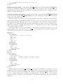
Example of a simple model for gene detection
Start(−)
Stop(+)
C
A
TCA
1
T
AGT
G
G
A
T
A
2
3
3
G
I
C
T
G
A
2
A
T
CDS(−)
A
C
G
intergenic
Stop(−)
AGT
T
T
Start(+)
G
1
CDS(+)
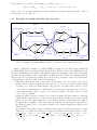
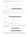
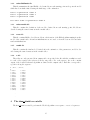
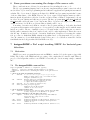
Fig. 1 – Example of a simple HMM dedicated to bacterial coding sequences detection
Figure 1 displays the structure of a simple HMM (represented by the hidden state transitions)
for which SHOW has been designed. Circles represent the considered states of the HMM and arrows
the allowed transitions between states. This graph modelises the alternation of intergenic regions with
CoDing Sequences (CDS) on the both strands of a DNA molecule. The model contains 23 hidden
states grouped in 7 groups (in dotted line). Here follows a short description of the biological meaning
of this graph (we only give details of the model structure).
– When the actual hidden state corresponds to an intergenic region at position t, the arrows
indicate that we can stay in this region at position t + 1 or leave it towards the first position
of a start codon on the (+) strand (triplets : atg, gtg, ttg) or towards a last position of a stop
codon on the (−) strand (inverse complementary of tga, tag, taa). Intergenic state can only be
reached from the last position of a stop codon on the (+) strand or the first position of a start
codon on the (−) strand.
– Leaving the third position of a start codon on the (+) strand, the hidden path goes through
a CDS which is a succession of codons. Codons are modelised by using a cycle of three hidden
states, one for each position inside the codon. This modelisation ensures that the length of
the CDS will be a multiple of three and enables to take into account distinct compositions of
the DNA according to the codon position (defined by the emission transitions b which are not
described here).
– At the third codon position on the (+) strand, it is necessary to forbid the appearance of an in
frame stop codon. Thus, the emission model associated with the third position needs to verify :
t−1
= tg) = 0, bCDS+ 3 (g; ta) = P (Xt = g | St =
bCDS+ 3 (a; tg) = P (Xt = a | St = CDS+ 3, Xt−2
t−1
t−1
= ta) = 0.
CDS+ 3, Xt−2 = ta) = 0 and bCDS+ 3 (a; ta) = P (Xt = a | St = CDS+ 3, Xt−2
4
– The first position of the stop codon on the (+) strand can only be reached from the third position
of a translated codon and corresponds to the first nucleotide of the triplets : tga, tag, taa.
– From the third stop codon position on the (+) strand, the path goes through intergenic.
– From the intergenic state, the third position of a stop codon on the (−) strand could be reached.
This transition enable the beginning of a CDS on the (−) strand.
In the next section, we will present the syntax allowing the definition of such HMM.
2.3
HMM specification file : -model <file>
Model specification consists in the specification of each hidden state (state and emission observation
transitions). It corresponds to the description of each of the nodes of the graph. This file does not
only contain the description of the model structure, but also indicates which parameters of the model
(b and a) are fixed or must be estimated when using the model as input of the show emfit executable.
When running show emfit, values found in this file for the parameters described as “to be estimated”
are used as the starting point of the iterative EM algorithm.
2.3.1
Hidden state definition
The HMM definition file is organized as a succession of hidden state definitions that makes it
highly modular, easy to edit by ’copy/paste’ operations and makes an existing model easy to extend.
The following shows an example of a hidden state which could be the intergenic hidden state of the
figure 1 definition :
BEGIN_STATE
state_id: intergenic
# identifier of the state
BEGIN_TRANSITIONS
type: 1
# allows estimation of the transition
state: start+_1
# transition towards start+_1 state
ptrans: 0.00432589
# probability of this transition
type: 1
state: stop-_3*1
ptrans: 0.00426073
type: 1
state: stop-_3*2
ptrans: 0.000892905
type: 1
state: intergenic
ptrans: 0.99052
END_TRANSITIONS
BEGIN_OBSERVATIONS
seq: genomic_dna
# a sequence id which must be the same as in the -seq <file>
type: 1
# allows estimation of the observation distribution
order: 2
# markov order of the observation distribution
pobs:
0.314514 0.183587 0.185804 0.316094
# a g c t
0.385992 0.177465 0.146873 0.28967
0.327029 0.217127 0.207901 0.247942
0.310991 0.158126 0.221846 0.309037
0.23778 0.185229 0.190936 0.386055
0.44321 0.181248 0.140779 0.234764
0.33124 0.25435 0.217354 0.197056
0.382986 0.161845 0.2005 0.25467
0.303587 0.204104 0.178921 0.313388
0.38761 0.202831 0.138278 0.27128
0.342915 0.224382 0.201373 0.231331
0.290107 0.172784 0.214286 0.322822
0.255216 0.193496 0.177495 0.373793
0.326314 0.198495 0.157725 0.317467
0.260414 0.258744 0.223338 0.257503
0.22166 0.186155 0.233092 0.359093
0.184989 0.211447 0.218147 0.385417
0.334371 0.134578 0.155746 0.375305
0.345444 0.155348 0.195448 0.30376
0.328272 0.126919 0.235736 0.309073
# aa ag ac at
# ga gg gc gt
# aaa aag aac aat
# gaa gag gac gat
5
0.204668 0.155128 0.192557 0.447647
END_OBSERVATIONS
END_STATE
# tta ttg ttc ttt
Hidden state description begins with the BEGIN STATE keyword and ends with the END STATE
keyword. It contains the identifier of the state that is used in the description of the outgoing transitions
and that must be unique. The state transition description is separated from the description of the
emission observation transitions.
Outgoing transition description from the hidden state begins with the BEGIN TRANSITIONS
keyword and ends with the END TRANSITIONS keyword. It contains the description of each allowed
transition from the hidden state.
The type : must be specified for each outgoing transition ; 0 means no estimation of the parameter
and 1 means estimation (by the EM algorithm). The state : refers to the identifier of the state to which
the transition is allowed. The ptrans : keyword preceeds a numeric value of the state outgoing transition
probability a(u, v). This numerical value is fixed when the type : is equal to 0, and corresponds to the
initial value required to run EM when the type : is set to 1 (in this last case, the value of ptrans will
evolve during iterations of EM).
The keyword label : can be set on the first line of the transition description. It enables to choose an
identifier which can be used with the keyword tied to : when setting up models with tied parameters.
The example below shows how to use this feature.
BEGIN_STATE
state_id: cds1+_3
BEGIN_TRANSITIONS
label: trans_cds+_3 # identifier is trans_cds+_3
type: 1
state: cds1+_1
ptrans: 0.99
type: 1
state: stop+_1
ptrans: 0.01
END_TRANSITIONS
BEGIN_OBSERVATIONS
seq: genomic_dna
type: 1
order: 2
pobs:
random
excepted: TGA TAG TAA
END_OBSERVATIONS
END_STATE
BEGIN_STATE
state_id: cds2+_3
BEGIN_TRANSITIONS
tied_to: trans_cds+_3
state: cds2+_1
# P(cds2+_3 -> cds2+_1) =
state: stop+_1
# P(cds2+_3 -> stop+_1) =
END_TRANSITIONS
BEGIN_OBSERVATIONS
seq: genomic_dna
type: 1
order: 2
pobs:
random
excepted: TGA TAG TAA
END_OBSERVATIONS
END_STATE
P(cds1+_3 -> cds1+_1)
P(cds1+_3 -> stop+_1)
In this example the states cds1+ 3 and cds2+ 3 correspond to the third codon position of a model
allowing two types of compositions for coding sequences. The outgoing transitions of this two states
are tied : they are identical and simultaneously estimated when running show emfit. This feature can
be used to ensure that the state transition probabilities will be the same for two or more hidden
states and can also be useful to decrease the number of parameters and then give an easier and better
estimation.
6
Observation emission transition probabilities description conditionally on the hidden state
begins with the keyword BEGIN OBSERVATIONS and ends with the keyword END OBSERVATIONS.
The first keyword found in the observation description must be seq : It gives an identifier that
must be the same as the identifier given in the file referenced by the -seq argument of the command
line (see the section 6 for more explanations).
The keyword type : indicates how the observation emission transition probabilities should be processed during estimation. Type 0 stands for no estimation (constant value) and type 1 means estimation.
Types 2 and 3 must be used only for tied observations : 2 means identical to the referenced observation
emission distribution, while 3 means complementary to the referenced one. Type 3 can only be used
when the order ru of the referenced observation emission distribution is 0. The observation emission
transition probabilities will be estimated when type is set to 2 or 3 only if the referenced one are
estimated.
The keyword order : is used to indicate the order r u of the markov chain of the observation emission
distribution. The keyword pobs : preceedes numerical
given by the user for the observation
Pru +1 values
−1
t
transition probabilities bu (x; x−ru ). After pobs :, t=1 4 numerical values
must be set to the values
−1
of bu (x; x−1
),
for
t
increasing
from
0
to
r
.
The
parameters
b
(x;
x
)
u
u
−t
−t 0≤t≤ru are used only at the
beginning of the sequence, i.e. when no sufficient context is known to use the parameters b u (x; x−1
−ru ).
These values correspond to the starting point required to process EM when type is set to 1, and are
fixed otherwise.
A random choice of the pobs values can be done by setting pobs : to the keyword random. In this
case, the model cannot be used directly for viterbi reconstruction of the hidden path or for simulation,
but must first be estimated using show emfit. Note that when using directly show viterbi or show simul,
the pobs : (and ptrans :) values will be considered as fixed for these executables, even if the type : of
these parameters is set to 1. Thus, show emfit must first be used to allow (some) parameter estimation.
Finally, the keyword excepted : can be used to forbid the emission of some words ; this keyword
was used in the previous example to forbid an in frame stop codon tag, tga and taa. The length of
the forbidden word must be ≥ ru + 1. If the length of a word lw forbidden by the excepted : keyword
is greater than ru + 1, then SHOW uses a special kind of Markov model for the observation emission
process. This Markov model corresponds to a model of order r u conditionally on that some words of
length lw do not appear, the resulting model is in fact a Markov model of order l w +1 but with the same
number of parameters than a Markov model of order r u . Then we refer to this kind of Markov model
as a Markov model of pseudo-order lw + 1. The following matrix gives an example of the parameters
of a Markov model of pseudo-order 1 corresponding to a Markov model of order 0 conditionally on
that ag dinucleotide does not appear.
bu (a)
bu (c)
bu (t)
0
b
(a)+b
(c)+b
(t)
b
(a)+b
(c)+b
(t)
b
(a)+b
(c)+b
(t)
u
u
u
u
u
u
u
u
u
b
(a)
b
(g)
b
(c)
b
(t)
0
u
u
u
u
bu (•; •) =
bu (a)
bu (g)
bu (c)
bu (t)
bu (a)
bu (g)
bu (c)
bu (t)
The example below shows how to use the keywords label : and tied to : in the observation description.
BEGIN_STATE
state_id: start+_1
BEGIN_TRANSITIONS
type: 0
state: start+_2
ptrans: 1
END_TRANSITIONS
BEGIN_OBSERVATIONS
seq: genomic_dna
label: start+_1_obs
type: 1
order: 0
pobs:
0.3 0.3 0 0.4 # a, g or t.
7
END_OBSERVATIONS
END_STATE
BEGIN_STATE
state_id: start-_1
BEGIN_TRANSITIONS
type: 0
state: intergenic
ptrans: 1
END_TRANSITIONS
BEGIN_OBSERVATIONS
seq: genomic_dna
tied_to: start+_1_obs
type: 3
END_OBSERVATIONS
END_STATE
2.3.2
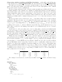
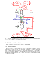
Two distinct modelisations of the boundaries of the sequence
SHOW allows two distinct modelisations of the sequence’s boundaries.
The first one enables to work conditionally on the length of the sequence. In this case the sequence
length is not modelised and the sequence begins and ends in any of the hidden states. This is the
default modelisation when no ’bound’ state is specified.
The alternative is to modelise the length of the sequence. This is done by imposing a state of which
the identifier is set to bound. The state named bound corresponds to the beginning and the end of the
sequence : the sequence begins when going out from the bound state and ends when reaching back
the bound state. No observations are described in the bound state description. The description of the
outgoing transitions from the bound state follows the same rules as any other state.
An application example of such modelisation is how to distinguish false and true sites corresponding
to some signals. When presenting a potential site, the likelihood of a true and false model is computed
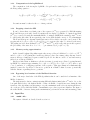
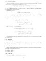
and the decision of predicting a true or a false site is taken according to the likelihood ratio. Figure 2
displays the graph corresponding to a HMM which can be used to predict a ten nucleotide length signal.
This model enables to take into account some kinds of correlations along the motif corresponding to
the signal. It could be learned using show emfit on a learning set. The prediction will be done by
computing the likelihood of the models corresponding to the true and false sites given the sequence
when running show emfit with the two models.
1
2
3
4
5
6
7
8
9
10
bound
Fig. 2 – Example of a HMM dedicated to a ten nucleotides length motif detection
The description of the beginning and the end of the model corresponding to the figure 2 is given
below.
BEGIN_STATE
state_id: bound # the ’bound’ state contains no observation description
BEGIN_TRANSITIONS
type: 1
8
state: motif_1*1
ptrans: 0.5
type: 1
state: motif_1*2
ptrans: 0.5
END_TRANSITIONS
END_STATE
BEGIN_STATE
state_id: motif_1*1
BEGIN_TRANSITIONS
type: 1
state: motif_2*1
ptrans: 0.5
type: 1
state: motif_2*2
ptrans: 0.5
END_TRANSITIONS
BEGIN_OBSERVATIONS
seq: genomic_dna
type: 1
order: 0
pobs: random
END_OBSERVATIONS
END_STATE
BEGIN_STATE
state_id: motif_1*1
BEGIN_TRANSITIONS
type: 1
state: motif_2*1
ptrans: 0.5
type: 1
state: motif_2*2
ptrans: 0.5
END_TRANSITIONS
BEGIN_OBSERVATIONS
seq: genomic_dna
type: 1
order: 0
pobs: random
END_OBSERVATIONS
END_STATE
.
.
.
.
BEGIN_STATE
state_id: motif_10*1
BEGIN_TRANSITIONS
type: 0
state: bound
ptrans: 1
END_TRANSITIONS
BEGIN_OBSERVATIONS
seq: genomic_dna
type: 1
order: 0
pobs: random
END_OBSERVATIONS
END_STATE
BEGIN_STATE
state_id: motif_10*2
BEGIN_TRANSITIONS
type: 0
state: bound
ptrans: 1
END_TRANSITIONS
BEGIN_OBSERVATIONS
seq: genomic_dna
type: 1
9
order: 0
pobs: random
END_OBSERVATIONS
END_STATE
2.4
Observed sequences file list : -seq <file>
The SHOW executables can work on a single sequence or a set of sequences. The sequences to
process are referenced in the -seq <file>. An example of such a file is given below. It must contain the
three keywords seq identifier, seq type and seq files.
seq_identifier: genomic_dna
seq_type: dna
seq_files:
ContigI.dna
ContigII.dna
Keyword seq identifier refers to any chosen identifier of the sequence, that must be the same as
in the -model <file> (keyword seq : in observation emission description). The seq type corresponds to
the nature of the observed sequence, currently only dna is properly supported. The seq files are the
name of the files containing sequences to be analyzed. Sequences in GenBank and Fasta format are
accepted. In order to process a sequence set, it is possible to store all the sequences in the same Fasta
file or to use multiple files, each of them referenced in the -seq <file>.
When processing a set of sequences, the sequences are considered as independent realisations of a
same HMM.
3
The show emfit executable
The show emfit executable simultaneously enables to estimate the parameters of the model by
likelihood maximization and to segment the sequence using the EM algorithm. The show emfit executable can also be used with fixed parameters to segment the sequences according to the Baum-Welch
algorithm or to compute the likelihood of a model for a given sequence.
3.1
EM algorithm / Baum-Welch algorithm
This section describes the EM algorithm implemented in SHOW. We denote by θ the whole parameters of the HMM (state and observation transitions a and b) that we want to estimate (some
parameters can of course be fixed). Given a starting value θ (0) of the parameters, the EM algorithm is
an iterative procedure that produces an approximation of the maximum likelihood estimation (MLE)
θ (m) that is updated at each iteration m. This procedure ensures the increase of the likelihood at each
iteration m : Pθ(m+1) (X) ≥ Pθ(m) (X).
EM consists in alternating two steps : the so-called E-step (for Expectation) and M-step (for Maximization).
3.1.1
E-step / forward-backward algorithm
The E-step on a HMM is also named Baum-Welch or forward-backward algorithm. It computes
the probability values Pθ(m−1) (St = u, St+1 = v | X1n = xn1 ) for each position of the sequence t ∈
[1, . . . , n − 1] and each couple of hidden states (u, v) ∈ [1, . . . , q] 2 . Values of Pθ(m−1) (St = u | X1n = xn1 )
are further deduced from Pθ(m−1) (St = u, St+1 = v | X1n = xn1 ).
10
The forward processing of the sequence starts with t = 1 and use recursively (t = 2, · · · , n)
both following equations until the calculation of the value P θ(m−1) (Sn = v|xn1 ) :
Predictive equation (1) :
if
t>1
Pθ(m−1) (St =
v|x1t−1 )
=
q
X
a(m−1) (u, v)Pθ(m−1) (St−1 = u | xt−1
1 )
u=1
else
Pθ(m−1) (S1 = v) = a(m−1) (v)
Filtring equation (2) :
(m−1)
Pθ(m−1) (St =
v|xt1 )
bv
= Pq
t−1
(xt ; xt−r
)Pθ(m−1) (St = v, | xt−1
1 )
v
(m−1)
t−1
)Pθ(m−1) (St
(xt ; xt−r
u=1 bu
v
(m−1)
For the first ru − 1 positions of the sequence, the probabilities b v
(m−1)
t−1
transitions bv
(xt ; xt−r
).
u
The backward processing of the sequence
the equations :
= u, | xt−1
1 )
(xt ; xt−1
1 ) are used instead of the
starts from t = n and use recursively (t = n−1, . . . , 1)
Smoothing equation (3) :
Pθ(m−1) (St−1 = u, St = v | xn1 )
=
a(m−1) (u, v)Pθ(m−1) (St−1 = u | x1t−1 )Pθ(m−1) (St = v | xn1 )
Pθ(m−1) (St = v | x1t−1 )
Equation (4) :
Pθ(m−1) (St−1 = u |
xn1 )
=
q
X
Pθ(m−1) (St−1 = u, St = v | xn1 )
v=1
3.1.2
M-step
M-step consists in updating the parameter θ by choosing
θ (m) = arg max Eθ(m−1) log Pθ (X1n , S1n ) | X1n
θ
i.e. the conditional expectation (to the current candidate θ (m−1) and the sequence X1n ) of the complete
loglikelihood. This maximization step uses the segmentation obtained during the E-step and leads to
the intuitive estimators.
Equation (5)
Pn
P (m−1) (St−1 = u, St = v | xn1 )
(m)
Pn θ
a (u, v) = t=2
n
t=2 Pθ (m−1) (St−1 = u | x1 )
and
bv(m) (x; w)
=
Pn
t=rv +1 Pθ (m−1) (St =
Pn
t=rv +1 Pθ (m−1) (St
v | xn1 )1{Xt =x,X t−1
=v|
t−rv =w}
n
x1 )1{X t−1 =w}
t−rv
In the special case of a state u with an observation emission Markov process with pseudo-order (See
Section ) the maximization of bu (. . .) could not be performed analytcally. Thus, this maximization is
performed using a multidimensional maximization routine of the GSL (GNU Scientific Library).
11
3.1.3
Computation of the loglikelihood
The computation of the incomplete loglikelihood is performed recursively (for t = 1, . . . , n) during
the E-step using equation :
log
Pθ(m−1) (X1t
=
xt1 )
= log
q
X
t−1
b(m−1)
(xt ; xt−r
)Pθ(m−1) (St = v|xt−1
v
1 )
v
v=1
+ log Pθ(m−1) (X1t−1 = x1t−1 )
Precautions must be taken for the rv − 1 first positions.
3.1.4
Stopping criteria for EM
It can be shown that every limit point of the sequence (θ (m) )m≥0 generated by EM (alternating
the E and M steps previously described) satisfies the incomplete log-likelihood equations and that
(θ (m) )m≥0 converges towards the maximum likelihood estimate (MLE) if the starting point θ (0) is not
too far from the true value. From a practical point of view, EM can thus converge to a local maximum.
The E and M steps are alternated until an iteration M for which convergence can be stated. The
stopping rule is | log Pθ(M +1) (X) − log Pθ(M ) (X)| ≤ , for a given (the value of is fixed by the user).
The parameters θ are then estimated by θ (M ) (a(M ) and b(M ) ), and for all positions t in the sequence,
the probability of the state St to be v = 1, · · · , q is estimated by Pθ(M ) (St = v | X).
3.1.5
Memory saving approximation
As the forward-backward algorithm requires the storage of the probabilities P θ(m−1) (St = u | X1t−1 )
and Pθ(m−1) (St = u | X1t ) during the forward step, this procedure can consume a large amount of active
memory when processing large sequences with a big model. A solution could be to use hard memory
(files) to store this probabilities.
Another solution that we think more effective in terms of execution speed have been implemented
0
in SHOW. It consists in approximating P θ(m−1) (St = u | X1n ) by Pθ(m−1) (St = u | Xss ) where s and
s0 are boundaries of overlapping segments of the sequence. This approximation is mathematically
justified because the dependence between two positions in a Markov chain decreases geometrically
with the distance separating the two positions.
3.1.6
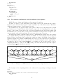
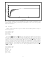
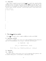
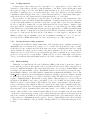
Bypassing local maxima of the likelihood function
One of the major drawbacks of the EM algorithm is that it can be stuck in local maxima of the
likelihood function.
The implemented solution consists in starting EM with distinct initial value θ (0) and to choose the
best path which leads to the highest likelihood value. As likelihood rapidly increases during the first
iterations of the algorithm, it is interesting to stop the maximization after a few iterations and then to
choose the model for which the likelihood maximization procedure is performed further. The figure 3
shows the likelihood increase during such a maximization performed from ten random starting points.
3.2
3.2.1
Input files
-model <file>
The syntax of this file is described in the section 2.3.
12
−133400
−133600
−133800
loglikelihood
−134000
0
50
100
150
iteration number
Fig. 3 – Example of likelihood increase during EM iterations. The loglikelihood maximization begins
with 10 starting points (during 50 iterations), only the likelihood of the best model is performed
further than 50 iterations
3.2.2
-em <file>
This file contains the information required to initialize and run the EM algorithm. An example of
such a file is given below.
estep_segment: 20000
estep_overlap: 1000
niter: 1000
epsi: 0.00001
Keywords estep segment and estep overlap refer to the length of the segment used for the memory
saving approximation during the forward-backward algorithm (E-step). For a given model and set
of sequences, the memory needed by the program grows linearly with estep segment. niter and epsi
define the stopping criteria of the EM-algorithm : EM iterations stop when the loglikelihood increase
between two consecutive iterations is lower than epsi or the maximal number of iterations niter has
been reached. If parameters of the emission observation process associated to some hidden states are
randomly initialized (i.e. model definition file contains pobs : random), supplementary keywords nb sel,
niter sel and eps sel are expected in the -em <file>. These supplementary keywords are used in the
following example.
estep_segment: 20000
estep_overlap: 1000
nb_sel: 3
niter_sel: 100
eps_sel: 0.01
niter: 1000
epsi: 0.0001
13
nb sel corresponds to the number of random starting points for the EM algorithm. niter sel refers
to the maximal number of iterations performed from each starting point. eps sel corresponds to the
stopping criteria of the EM algorithm running from each starting point.
3.2.3
-seq <file>
The syntax of this file is described in the section 2.4.
3.2.4
Optional -output <file>
This file is optional and is required for the output .e file generation. The -output <file> contains
the output of the last iteration I of the forward-backward algorithm, i.e. the probabilities P θ(M ) (St =
u | X1n ) and Pθ(M ) (St = u, St+1 = v | X1n ) for each state u, v and each position t of the sequences. An
output file containing these probabilities for all considered states can be very large and difficult to use
and analyze. Then, a summary of selected states can be done.
The following example gives the syntax of such an output .e file :
(rhom1) (rhom2 ; rhom3) (rhom2 -> rhom3)
If rhom1, rhom2, rhom3 are three (hidden) states, the output file will contain three columns (of length
n) corresponding to Pθ(M ) (St = rhom1 | X1n ), Pθ(M ) (St = rhom2 | X1n ) + Pθ(M ) (St = rhom3 | X1n )
and Pθ(M ) (St = rhom2, St+1 = rhom3 | X1n ). Note that a same probability cannot be summed in two
columns.
3.3
Output files
Some files are created in the current directory when running show emfit. The names of these files
are generated by adding suffixes to the name of -seq <file>, excepted output files with the suffix .e
which are created using the names of the individual sequence files referenced in -seq <file>. Files with
suffixes containing .select are generated only if random initializations of the EM-algorithm are used.
Files with the suffix .e are generated only if an -output <file> is specified.
3.3.1
.select.traces file
This file contains likelihoods of the models at each iteration of the EM-algorithm running from
each starting point.
****************************************
model 0
iter 0 logl -71378.6
iter 1 logl -68449.2 diff 2929.44
iter 2 logl -68067.4 diff 381.803
iter 3 logl -67971.1 diff 96.317
iter 4 logl -67928.4 diff 42.6526
iter 5 logl -67903.5 diff 24.9115
iter 6 logl -67886.6 diff 16.8449
iter 7 logl -67874.3 diff 12.3817
iter 8 logl -67864.8 diff 9.50504
iter 9 logl -67857.3 diff 7.44326
iter 10 logl -67851.4
****************************************
model 1
iter 0 logl -71490.3
iter 1 logl -68347.4 diff 3142.88
.
.
.
14
3.3.2
.select.likelihoods file
This file summarizes the final likelihoods obtained from each starting point and reports the model
which has been further fitted during the final stage of the estimation.
model 0 loglikelihood -67851.4
model 1 loglikelihood -67883.3
model 2 loglikelihood -67901
best model found 0 loglikelihood -67851.4
3.3.3
.select.models file
This file contains the definition of the models obtained from each starting point ; Models are
described using the same format as in the -model <file>.
3.3.4
.trace file
This file contains likelihoods of the models at each iteration of the EM-algorithm running from the
model of the -model <file> if random initializations are not used or from the best model found after
random initializations.
3.3.5
.model file
This file contains the final model obtained after the estimation of the parameters ; model is described using the same format as in the -model <file>.
3.3.6
.e file
These files are only generated if an -output <file> is specified. One file with the .e suffix is created
for each of the sequence files referenced in the -seq <file>. For each sequence, the .e file contains
output of the forward-backward algorithm as defined in the -output <file>. Each line corresponds to
a position along the sequence.
# ( hello ) ( hello2 )
#
0.209391
0.790609
0.174707
0.825293
0.0927552
0.907245
0.081693
0.918307
0.0806847
0.919315
0.125776
0.874224
0.161663
0.838337
0.235672
0.764328
0.221932
0.778068
0.178636
0.821364
0.114087
0.885913
0.0881827
0.911817
0.0877433
0.912257
0.0741231
0.925877
.
.
.
4
The show viterbi executable
The show viterbi executable performs the Viterbi algorithm on a sequence or a set of sequences.
15
4.1
Viterbi algorithm
The Viterbi algorithm enables the computation of the most likely hidden state path s ? given the
observed sequence xn1 and the model parameters θ = (a, b) :
s? = arg max
Pθ (S1n = sn1 | X1n = xn1 ) = arg max
Pθ (S1n = sn1 , X1n = xn1 )
n
n
s1
s1
To overcome numerical problems, we present a version of Viterbi by taking the logarithm of all the
probabilities involved in the algorithm.
Starts with t = 1 with :
log Pθ (S1 = v, x1 ) = log(bv (x1 )a(v))
For t increasing from 2 to n − 1, compute by recurrence the logarithm of the maximal probability
of the most probable path (enabling to generate the observations x 1 , . . . , xt+1 ) that ends in position
t + 1 in state St+1 = v :
max log Pθ (S1t = st1 , St+1 = v, xt+1
1 )
st1
= max log(bv (xt+1 ; xtt−rv +1 )a(u, v)) +
u
max log Pθ (S1t−1 = s1t−1 , St = u, xt1 )
st−1
1
Find s? = (s?1 , s?2 , . . . , s?n ) by backtracing :
s?n = arg max max log Pθ (S1n−1 = s1n−1 , Sn = v, xn1 )
v
sn−1
1
s?t = arg max log(bv (xt+1 ; xtt−rv +1 )a(u, s?t+1 ))
u
+ max log Pθ (S1t−1 = s1t−1 , St = u, xt1 )
st−1
1
The same memory saving approximation has been implemented as for forward-backward algorithm
(See section 3.1.5).
4.2
4.2.1
Input files
-model <file>
The syntax of this file is described in the section 2.3.Keep in mind that all the parameters of the
model must be fully specified, i.e. the file must not contain any pobs : random.
4.2.2
-vit <file>
This file contains the information concerning the parameters of the memory saving approximation.
An example of such a file is given below.
vit_segment: 20000
vit_overlap: 4000
4.2.3
-seq <file>
The syntax of this file is described in the section 2.4.
16
4.3
Output files
Only one kind of output file is generated by the show viterbi executable. One output file with the
.vit suffix is created for each sequence file referenced after the seq files keyword in the -seq <file>. For
each sequence file, the .vit output file contains the most probable hidden path. An example of such a
file is given below : the mapping between numbers and hidden state identifiers is given in the header
of the file, each line of the file corresponds to a position along the sequence (excepted in the header).
# viterbi reconstruction
# 0 : (hello) 1 : (hello2)
0
0
0
0
0
0
0
0
0
0
0
0
0
0
0
.
.
.
0
0
0
1
1
1
1
.
.
.
The show simul executable
5
The show simul executable enables to simulate an HMM given a fully specified HMM.
5.1
Simulating an HMM
The simulation of an HMM is easy because it only consists in simulating the hidden path given its
markov model and simulating the observed sequence conditionally on the hidden path :
S1 ∼ M1 (a(1), a(2), . . . , a(q))
St | St−1 = u ∼ M1 (a(u, 1), a(u, 2), . . . , a(u, q))
t−1
t−1
t−1
t−1
Xt | St = v, Xt−r
= xt−r
∼ M1 (bv (1; xt−r
), bv (2; xt−r
), . . . , bv (4; xt−1
t−rv ))
v
v
v
v
5.2
5.2.1
Input files
-model <file>
The syntax of this file is described in the section 2.3. Keep in mind that all the parameters of the
model must be fully specified, i.e. the file must not contain any pobs : random.
17
5.2.2
-simul <file>
This file contains only the length of the sequence to be simulated.
lg: 10000
5.2.3
-seq <file>
The syntax of this file is described in the section 2.4. It may surprise that such a file should be used
by a sequence simulation program. However, the sequence referenced in this file is absolutely not used
for the simulation of the new sequence, but the seq type information of the -seq <file> is necessary.
5.3
Output files
5.3.1
simulated.hidden states file
This file conforms to the same format as output files of the show viterbi executable. An example of
such a file is given below.
# hidden states simulation
# 0 : (state1) 1 : (state2)
1
1
1
1
1
1
1
1
2 : (state3)
3 : (state4)
.
.
.
1
1
1
3
3
3
.
.
.
5.3.2
simulated 0.dna file
A DNA sequence in Fasta format.
> dna observations simulation
TTAGATCAAAAACAGCAGGTAAATAAAAGTTCTATTACTGAAGCGAAGGTGTTTCAACAC
CAAAAATGTTCTAAGGATATTCCTGACCTTAGTGGACAGCATCAAATGATATCTTTTCAT
GCAAATATACAAGTCTAGAAAAATTATTCATTTAATTGCAAAACTAGAAGGCTTTTTCTG
CCAGCGCCTACTAAGAATGGGCAAGTTCGTTAAACTTAAGATGGTACAAAGGTTTCTTTG
GCACAAGTGTGCTTATTTTATGCTAGATGAATTCCTTACATACTATGATAATCTTTGTTT
ATCAGATGACGGTAATAGTATTTGTCAAGTTTTCTCTTTAGGAAGAACTATCACTTGATT
.
.
.
If the model includes a “bound” state, the output sequence is a concatenation of sequences of
total length corresponding to the length specified in -simul <file>. Appearances of “bound” states
delimit individual sequences, “bound” state positions along the concatenated sequence is given in the
simulated.hidden states file in the same way than other hidden states, and in the simulated 0.dna file
by “X” in the simulated sequence.
18
6
Some precisions concerning the design of the source code
These considerations are dedicated to users interested in extending the source code.
The C++ programming language has been chosen to implement this program because it is widely
used, it allows object-oriented programming and it is efficient for applications requiring intense numeric
calculus. The object-oriented design is well adapted for HMM based programs in particular because
of the modular nature of the HMM. However, an object oriented design implies numerous calls to
function (methods) and then could slow down the execution. Thus, a balanced design must be chosen
in order to keep modularity and efficiency properties. The three programs show emfit, show viterbi and
show simul share widely the same object components. These objects are well designed for some further
extensions but not for all. Here we present what we think possible or not.
Concerning observation modelisation, extends of the program enabling to deal with other kinds
of sequences such as amino-acids sequences, codon sequences (conditioning the model with the translation) are possible. The use of multiple sources of observation that could be taken into account for
hidden path reconstruction has been considered and could be easily implemented. This is the reason
why the seq : identifier is used in the observation distribution description. Concerning the estimation procedure we think that HMM estimation algorithm based on bayesian methodology could be
done. In contrast, we do not think that the design of the source code could allow extension to hidden
semi-Markovian models (generalized hidden Markov model).
7
7.1
bactgeneSHOW a Perl script invoking SHOW for bacterial gene
detection
Motivation
SHOW is a generic program that uses various HMMs to analyze biological sequences (especially
DNA). The design of the HMM and the processing of the output files is a sizeable task. Thus we
propose a Perl script that enables to use SHOW for bacterial gene detection using a single command
line.
7.2
The bactgeneSHOW command line
Usage: bactgeneSHOW -i <dnafile> -o <outputfile> [options]
<dnafile>
Fasta file containing the DNA sequences to be analyze
<outputfile> Annotation file containing the results of the gene detection
OPTIONS:
1- CHOICE OF THE MODEL AND PARAMETERS ESTIMATION
-m
<modelid>
1c | 2c | 3c | 4c | 1c_si | 2c_si | 3c_si | 4c_si
Number of coding types to use; "si" stands for short
intergenic (default is 4c_si).
-rna
<rnafile>
Optional fasta file containing DNA sequences
of structural RNA genes (used only in order
to compute nucleotides frequencies).
-rbs
<modelid>
m0 | m1 | double_m0 (default is m0).
-em
<niter epsi niter_sel nb_sel eps_sel>
Parameters for the EM algorithm
(default is 20 0.01 50 10 10).
2- USE OF AN ALREADY ESTIMATED MODEL
-fm
<showmodel> A bacterial gene detection model already fitted by SHOW.
If used, any option of the SECTION 1- is ignored.
3- TEMP FILES AND PARAMATERS OF THE GENE PREDICTION OUTPUT
-d
<tmpdir>
Location of the "temporary" directory where SHOW I/O
used by the Perl script will be located
(default is /tmp/).
-cdst
<float>
Probability threshold for CDS prediction (default is 0.5).
-startt <float>
Probability threshold for multiple starts prediction
(default is 0.1).
-rbst
<float>
Probability threshold for RBS prediction (default is 0.1).
19
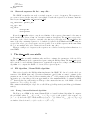
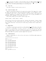
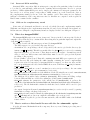
G
2;3
AorGorT
A
T
2;1
G
T
A
3;2
G
1;2
G
Overlaps +/+
3;1
G
T
A
2
1;3
T
A
AorGorT
G
1
3
2
2
3
1
3
Coding +
Overlap +/− 2nt
G
Start+
T
T
A
AorTorG
Stop+
G
G
A
TorC
RBS−
Intergenic
T
RBS+
A
Stop−
T
C
TorAorC
C
T
A
A
AorG
Start−
C
Coding −
3
1
2
2
3
1
2
C
3;1
3
1
TorCorA
T
A
C
A
T
C
T
A
C
A
2;1
C
2;3
1;2
1;3
1;3
noT
TorAorC
T
3;2
C
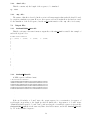
Fig. 4 – Structure of a HMM dedicated to bacterial coding sequences detection used by bactgeneSHOW.
Colors are used in text in order to identify parts of the model.
7.3
HMM for bacterial gene detection
Figure 4 displays the structure of the models used by bactgeneSHOW.
7.3.1
Intergenic sequences
Intergenic sequences are modelled using a single back looped hidden state, emitting the observed
DNA sequence according to a second order Markov chain. The structure of the model displayed in
Figure 4 contains a single intergenic state (at the center of the graph). However, if -m <modelid>
refers to a model identifier containing “si” (short intergenic), two supplementary states are added for
short intergenic regions modelling. The purpose of the use of these states is explained in the paragraph
concerning RBS modelling.
20
7.3.2
Coding sequences
Coding sequences have a three-periodic composition “core”, represented by a cycle of three hidden states, corresponding to the three positions within a codon. Each of these hidden states emits
nucleotides according to a second order Markov chain. In frame stop codons are prevented by a zero
probability of emitting a stop codon in the third state of the cycle. All states concerned with this
constraint are filled in Figure 4. In order to ensure that start and stop codons delimit CDSs, appropriate sub-models are added upstream and downstream from the core of the CDS.
Heterogeneities of coding sequences composition have been shown to be important features of the
bacterial chromosome composition. In particular, taking into account the atypical a+t-rich composition
of some horizontally transferred genes has been shown to greatly improve gene detection sensitivity.
In order to take these features into account, different sub-models corresponding to distinct coding
types are reachable downstream from a start codon. Moreover, composition type can change within
genes. This is more general than using disjoint gene types, and also more realistic, in particular with
regard to the existence of hydrophobic regions in proteins. The model displayed in Figure 4 contains
two types of coding regions. The user can choose the number of coding sequence compositions of the
HMM according to the -m <modelid> option. Model identifiers containing “1c”, “2c”, “3c” and “4c”
refer respectively to HMM with a single, two, three and four types of coding compositions.
7.3.3
Overlap between coding sequences
Overlaps between CDSs are an important feature of the bacterial genome organization. Our model
distinguishes the very frequent short overlaps of 1, 2 or 4 nucleotides from the rare longer overlaps.
Composition of long overlaps is modelled in the same way as non overlapping CDSs. As not so much
data is available in a single genome for their composition estimation, we use for these overlaps an
emission process of order 1. In order to prevent from the appearence of in frame stop codons we used a
pseudo-second order model, corresponding to a Markov model of order 1 conditionally on the absence
of stop codons. Hidden states and transitions used to model the overlaps are colored in red in Figure 4.
7.3.4
RBS modelling
Taking into account that the ribosome binding site (RBS) position has been shown to improve
precise start site prediction, this can also help to predict short genes where CDS composition does
not provide sufficient information. The script enables the user to choose between distinct RBS models
according to the -rbs <modelid> options : -rbs m0 RBS sequences are modelled by a positional compositional matrix of Markov order 0 and length 14 ; -rbs m1 same as -rbs m0 but with Markov order 1 ; -rbs
double m0 the positional compositional matrix is duplicated enabling to model two distinct consensus
for RBSs (proposed in Besemer et al., Nucleic Acids Res., 2001). The RBS is followed by a “spacer”
sequence of minimal length 1. Hidden states corresponding to RBS and spacer are colored in blue in
the Figure 4. The HMM does not enforce each CDS to be preceeded by RBS : the probability to find a
RBS before a start codon is estimated. The addition of two states corresponding to “short intergenic”
regions could improve this estimation. These two states are the same as the central intergenic state
in terms of composition (tied observations) but their transitions differ. They are dedicated to model
short intergenic regions, separating CDSs on the same strand : one for CDSs on the forward strand
and the other for CDSs on the backward strand. RBS model is not reachable from the state which
corresponds to short intergenic regions on the forward strand (reciprocally, short intergenic regions
state is not reachable from RBS model on the backward strand). One of the main interest of the use
of these states is to distinguish intergenic regions too short to contain RBS from the others, and thus
to enable a better estimation of the probability of finding a RBS before a CDS when intergenic is not
so short.
21
7.3.5
Structural RNA modelling
Structural RNA composition differ from intergenic composition. In particular, it has been shown
to be related to environmental conditions for the organism, such as temperature. In order to prevent
prediction of CDSs within rRNA genes, and to improve the estimates for intergenic parameters, the
user can choose to add two states corresponding to rRNA texture (one on the forward, the other on
the complementary strand) by the use of the -rna <rnafile> option. These states are not displayed
in Figure 4. Parameters of the composition associated to this state are computed on the sequence in
Fasta format contained in the <rnafile>.
7.3.6
CDSs on the complementary strand
Genes exist on both strands, and therefore are read on both the direct and complementary strands.
With minor modifications, the complementary strand model can be derived from the direct strand one,
hidden states modelling the complementary strand are displayed in the lower half part of Figure 4.
7.4
What does bactgeneSHOW ?
The bactgeneSHOW script creates a new “temporary” directory in the location specified by the -d
<tmpdir> option. This directory contains all the intervening files, in particular input and output files
of the show emfit executable.
We will now describe the different steps performed by bactgeneSHOW.
– The DNA sequence is copied in the temporary directory.
– An initial model corresponding to the model specified by the user is copied in the directory (for
instance gene 4c si.model). This file is a -model <file> for show emfit (see section 2.3) containing
flags between { and } or between two !. These flags are used by the script to determin respectively
where to add some hidden states and which states must be used for gene prediction (states
modelling coding regions).
– If -rna <rnafile> option is used, Fasta file containing structural RNA gene sequences is copied
in the directory and a file having the suffix .invcomp containing the reverse complementary
sequences is created. Composition of structural RNA is computed over these two files, and the
two corresponding states are added in the HMM ; the new model file have rna prefix (for instance
rna gene 4c si.model).
– Input files for show emfit are created : em.desc (see section 3.2.2) according to the -em <niter
epsi niter sel nb sel eps sel> option, start.set (see section 2.4).
– show emfit estimates the parameters of the initial model, the following files are created : start.select.traces,
start.select.likelihoods, start.select.model, start.trace, start.model (see section 3.3).
– The initial model is enriched after estimation (start.model), hidden states modelling overlaps
between CDSs and RBS are added, the resulting model file is named startbis.model.
– show emfit estimates the parameters of the enriched model (startbis.model), it produces the
output files : final.select.traces, final.select.likelihoods, final.select.model, final.trace, final.model (see
section 3.3). The file final.model contains the final fitted model which will be used for gene
prediction.
– An output description file named outputfromparse.desc (see section 3.2.4) is created by parsing
final.model according to the flags between two !.
– show emfit performs forward-backward algorithm (using the files final.model, outputfromparse.desc
and em final.desc) and produces an output file with suffix .e (see section 3.3.6).
– The .e output file is parsed to produce the annotation file, either in GFF format or in GenBank
feature format.
7.5
How to retrieve a fitted model for use with the -fm <showmodel> option
Copy the file named final.model from the temporary directory created during a preceding run of
bactgeneSHOW.
22
8
Acknowledgments
We thank Antoine Marin, Gregory Nuel and Vincent Miele for their help in accessing powerful
computers which enables us to try numerous HMM for varied biological problems. We are grateful to
Mark Hoebeke for advices in C++ object-oriented development, which unfortunatly have not always
been followed !
23