Download QeCode User Manual - Université d'Orléans

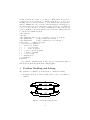
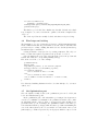
QeCode User Manual
Manual v0.2.1 documenting QeCode v2.0.1
Marco Benedetti, Arnaud Lallouet, J´er´emie Vautard
University of Orl´eans - LIFO
mailto:[email protected]
May 5, 2009
1
Before you start
QeCode is a C++ library designed to express and solve Quantified Constraint
Satisfaction Problems (QCSP) and Quantified Constraint Optimization Problems (QCOP). QeCode provides an extended modeling language with the support of restricted quantification. QeCode relies on the finite domain constraint
solving library GeCode [3].
This manual assumes that QeCode and its examples compile well. See the QeCode webpage and the ”COMPILING” file in the examples folder to know how
to compile QeCode. Moreover, while Quantified CSP (and QCSP + ) are briefly
explained, this guide is not intended to explain all the subtleties of quantified
problems modeling, but to get started with QeCode quickly.
It is assumed that you have a fair knowledge of finite domains constraint programming, and some bases in the C++ language.
2
2.1
A Quick QCSP + and QCOP+ Overview
QCSP+
Solving a CSP is equivalent to answer to the question ”does it exists an assignment of all the variables of the problem such that every constraint is satisfied ?”,
which, for a CSP composed of n variables and m constraints, is expressed in
logic by the following formula :
∃x1 ∃x2 . . . ∃xn . c1 ∧ c2 ∧ . . . ∧ cm
The QCSP + framework allows to model problems of the following form:
Q1 x1 [C1 ]
Q2 x2 [C2 ]
...
Qn xn [Cn ]
G
where, for i ∈ [1..n], Qi is a quantifier, either ∃ or ∀ and xi is a set of finite
domain variables. The set Ci is a CSP which restricts the possible values of
previously defined variables to the only values which are consistent with the
constraints. We call this block Qi xi [Ci ] a restricted quantified set of variables
or rqset. Finally, G is a CSP called goal which has to be satisfied by any
assignment satisfying the previous rqsets. The bracket notation for the CSP Ci
is a generic notation read as ”such that”. It yields that the rqset is linked to the
rest of the formula by ∧ if the quantifier is ∃ and by rightarrow if the quantifier
is ∀. For example, the formula:
∃x∀y[x 6= y]∃z[z < x].z < y
is read logically as:
∃x∀y.(x 6= y) → ∃z.(z < x) ∧ (z < y)
2
Technical details on QCSP + can be found in [1].
The original QCSP framework [2] did not provide the restricted quantifiers.
The QCSP + formalism has been designed to overcome the difficulty to model
problems like games where the possible moves of each player depends on what
has been played before. For example, let us consider two simple games, the Nim
game and a variant called ”Nim-Fibonnaci”:
The Nim game consists in a set of n matches, from which each player takes
in turn from one to three matches. The player who takes the last match is the
winner. Deciding if the first player has a winning strategy for this game can be
easily modeled in classical QCSP :
∃x1 ∈ [1..3]∀y1 ∈ [1..3] . . . ∃xn/4
(
n/4
X
xi + yi = n)
i=1
The Fibonnaci variant of the Nim game has slightly different rules: the first
player can remove as many matches as he wants, though without emptying the
set. Then each player in turn can take up to twice the number of matches its
opponent has taken in the previous turn. This implies that it is impossible to
know in advance how many matches one player will be allowed to take at a
given time. In QCSP + , this can be naturally represented :
∃x1 ∈ [1..n − 1]
∀y1 ∈ [1..n − 1] (y1 ≤ 2x1 ) ∧ (x1 + y1 ≤ n) →
∃x2 ∈ [1..n − 1] (x2 ≤ 2y1 ) ∧ (x1 + y1 + x2 ≤ n) ∧
...
>
Note that the aim of the game is directly modeled by the (x1 + y1 + . . . ≤ n)
constraints: actually, if one player empties the set, his opponent will have no
way to move, and so he will loose the game (if the first player takes the last
match, the rest of the formula is reduced to ∀y ⊥ → (. . .) which is obviously
true, and if the second player takes the last match, the rest of the formula is
reduced to ∃x ⊥ ∧ (. . .) which is obviously false). Thus, the goal is not needed
in this example, and is therefore set to true.
2.2
QCOP+
QCOP+ are an extension to QCSP+ that allows to define an optimization condition at each existential scope. In this kind of problems, each existential scope
represents a different player, which tries to optimize its own parameter : First
player fixes its own variables, according to what she wants to optimize, but
knowing that the second player will act accordingly to it own criterion, and so
on.
Let us take the example of a network pricing problem : thi problem consists
in setting a tariff on some network links in a way that maximizes the profit
of the owner of the links (the leader). The network, as depicted in Figure
1, is composed of N Customer customers (the followers) that route their data
independently at the least possible cost. Customer i wishes to transmit di
3
amount of data from a source xi to a target yi . Each path from a source to
a target has to cross a tolled arc aj . On the way from si to aj , the cost of
the links owned by other providers is cij . It is assumed that each customer i
wishes to minimize the cost to route her data and that they can always choose
an other provider at a cost ui . The purpose of the problem is to determine the
cost tj to cross a tolled arc aj in order to maximize the revenue of the telecom
operator. In Figure 1, there is 2 customers and 3 tolled arcs. This problem can
be expressed as a QCOP as follows:
const NCustomer
const NArc
const c[NCustomer,NArc] // c[i,j] = fixed cost for Ci to reach Aj
const d[NCustomer]
// d[i] = demand for customer i
const u[NCustomer]
// u[i] = maximal price for customer i
\exists t[1], ..., t[NArc] in [0,max]
| \forall k in [1,NCustomer]
| | \exists a in [1,NArc],
| | |
cost in [1,max],
| | |
income in [0,max]
| | | cost = (c[k,a]+t[a])*d[k]
| | | income = t[a]*d[k]
| | | cost =< u[k]
| | minimize(cost)
| s:sum(income)
maximize(s)
Note that the optimization part is only composed of the last three lines of
this expression. Removing them yields a simple QCSP+ .
3
Problem Modeling and Solving
The declaration of a QCSP + problem in QeCode consists in declaring:
1. how many rqsets the problem contains, and for each one, its number of
variables
Figure 1: A network pricing problem
4
2. For each rqset :
• the domain of each of its variables
• its constraints
3. the constraints of the goal.
QeCode provides a set of methods which allows to perform each of these steps
in the order they are described.
3.1
Headers and preliminary definitions
Let us write the code that solves the QCSP + corresponding to the network
pricing example given above (without considering the optimization part), with
2 clients, and 3 links.
Qecode is a C++ library that you have to link against. To use this library,
here are the different headers you need to include:
• QCOPPlus.hh contains all the necessary to create quantified problems. The
file itself includes the Gecode minimodel file which is needed to post the
most common constraints.
• qsolver general.hh contains the solver class.
These two files have to be included for modeling and solving the example above.
An object of the class Implicative represents a QCSP + problem. The only
public constructor must be given several parameters:
• the number of rqsets the problem contains (integer),
• an array of booleans specifying the quantifier associated to each rqset (true
for universal, false for existential),
• an array of integers containing the number of variables for each rqsets,
In our example, the parameters will respectively be 3, {true,false,true},
{3,1,9} : 3 rqsets, the first being existentially quantified. The first scope
have one variable by link, the second one only one variable which identificates
the client, and the last scope contains the cost and income variables, plus some
auxiliarly variables that are needed to calculate them. Here is the corresponding
C++ code:
#include "qsolver_general.hh"
#include "QCOPPlus.hh"
int main() {
int NArc = 3;
int scopeSize[] = {3,1,9};
bool quants[] = {false,true,false};
Qcop p(3,quants,scopeSize);
5
3.2
Variables domains
The Implicative object (that has been named p in the code) provides several
methods that allow to declare the type and the domains of the variables :
• qIntVar(int v, int min, int max) specifies that variable number v is
an integer variable whose domain is ranging from min to max
and, for a boolean variable:
• qBoolVar(v) specifies that variable v is a boolean variable.
3.3
Posting constraints and branching heuristics in rqsets
and the goal
Posting the different contraints and branchings of a QCSP + is done in the
order of the rqsets, followed by the goal. After its creation and declaration of
all the variables, the Implicative object is ready to accept constraints for its
first rqset. It provides methods to return all the objects required for posting
constraints and branchings in GeCode style:
• the space() method returns a pointer to the current Gecode::Space object
• the var(int i) (resp. bvar(int i)) method returns an IntVar (resp. a
BoolVar) corresponding to the i-th variable of the problem.
Note that you MUST declare your variables (using the qIntVar or qBoolVar
method) BEFORE using them (with the var or bvar methods) in constraint or
branching declaration, or Qecode will exit with an error message. Also, beware
that not properly posting a branching on each scope will most likely yield a
wrong answer from Qecode.
After having posted constraints and branchings in the current rqset, it is
needed to call the nextScope() method to go to the next level of the formula.
It yields that the next constraints will be posted in the next rqset, and eventually
in the goal. The code for declaring all the constraints of the first two scopes of
our example is:
// First quantifier
for (int i=0;i<NArc;i++)
problem.QIntVar(i,0,10); // t[i]
IntVarArgs branch1(NArc);
for (int i=0;i<NArc;i++)
branch1[i] = problem.var(i);
branch(problem.space(),branch1,INT_VAR_SIZE_MIN,INT_VAL_MIN);
problem.nextScope();
// Second quantifier
problem.QIntVar(NArc,0,NCustomer-1); // k
IntVarArgs branch2(NArc+1);
6
for (int i=0;i<NArc+1;i++)
branch2[i] = problem.var(i);
branch(problem.space(),branch2,INT_VAR_SIZE_MIN,INT_VAL_MIN);
problem.nextScope();
The third scope is declared in a similar way, but this declaration is a little
long. Complete code can be found in the ”optim2.cc” file in the examples folder
of Qecode.
The decision problem is now fully declared and almost ready for solving.
3.4
Final steps and solving
The last thing to do before solving the problem is to call the makeStructure()
method which checks that the problem has been well declared, and makes the
problem ready for solving. Calling this method is not absolutely mandatory,
but still strongly recommanded.
Solving an instance of Qcop is done by creating a QSolver. The only constructor of this class requires as parameter the problem to be solved.
Once the QSolver is created, the solve() method solves the problem and
returns, if it exists, the corresponding winning strategy.
Here is the end of the code of the example:
p.makeStructure();
QSolver s(&p);
long number_of_nodes=0; // for statistic purposes
Strategy solution = s.solve(number_of_nodes);
if (!solution.isFalse())
cout << "Problem is true !" << endl;
else
cout << "Problem is false !"<<endl;
cout << "Number of nodes encountered :" << nodes << endl;
return 0;
}
Note that any branching heuristic from Gecode works with Qecode, even userdefined ones.
3.5
the Optimization part
Once the QCSP+ is fully declared, the optimisation part can be added just
before the makeStructure() call.
In the optimization part, each existential scope is assigned an Optimization
variable to be minimized or maximized. An optimisation variable can be either
an existential variable of the problem, or an aggregated value calculated at a
given universal scope. In our example, the optimization variable of the last scope
is an existential variable (costOpt), while the first scope aims at maximizing the
sum of the values taken by the income variable for each branch of the second
(universal) scope. This is represented by an Aggregate, which is composed of an
7
optimization variable (here, the Income existential variable, and of an aggregator
function (here, the sum).
Note that the way from an existential scope and its optimization variable
must not go through a universal scope : for example, it would not make sense in
the first scope to optimize directly the Income existential variable (which belong
to the third scope).
The code corresponding to the optimization part is :
OptVar* costopt = problem.getExistential(NArc+2);
OptVar* incomeopt = problem.getExistential(NArc+3);
problem.optimize(2,1,costopt); // at scope 2, we minimize (1) the variable "cost"
AggregatorSum somme;
OptVar* sumvar = problem.getAggregate(1,incomeopt,&somme);
// sumvar represents the sum of the income for each client
problem.optimize(0,2,sumvar);
Again, this piece of code comes just before the problem.makeStructure() call.
3.6
solving the problem
Once the QCOP+ problem is fully defined, the last thing to do is to call the
solver. It is an object of the class QSolver which only constructor requires a
reference to the problem to be solved as parameter :
QSolver sol(&problem);
The solver being initialized, the solve method will solve the problem and
return the optimal winning strategy. In case the problem is unsat, the ”trivially
false” strategy is returned. The solve method requires one parameter : a reference to an unsigned long int that will be incremented by the number of nodes
encountered :
unsigned long int nodes=0;
Strategy outcome = sol.solve(nodes);
The strategy is a tree that can then be explored. See for example the PrintStr
strategy output method.
The complete code of this example can be found in the file examples/optim2.cc.
References
[1] Marco Benedetti, Arnaud Lallouet, and J´er´emie Vautard. QCSP Made
Practical by Virtue of Restricted Quantification. In Manuela Veloso, editor, International Joint Conference on Artificial Intelligence, pages 38–43,
Hyderabad, India, January 6-12 2007. AAAI.
[2] Lucas Bordeaux and Eric Monfroy. Beyond NP: Arc-consistency for quantified constraints. In Pascal Van Hentenryck, editor, Principles and Practice
of Constraint Programming, volume 2470 of LNCS, pages 371–386, Ithaca,
NY, USA, 2002. Springer.
8
[3] Gecode Team. Gecode: Generic constraint development environment, 2006.
Available from http://www.gecode.org.
9
Manual revisions
• v0.2.1: class names changes in last version of QeCode.
• v0.2: documenting Qecode2, introducing QCOP+.
• v0.1.2: improves QCSP+ introduction, full source code of the example.
• v0.1.1: overview, how to declare a QCSP+ formula, how to post constraints, a simple example.
10