Download ASP modulo CSP: The clingcon system

Under consideration for publication in Theory and Practice of Logic Programming
1
arXiv:1210.2287v1 [cs.LO] 5 Oct 2012
ASP modulo CSP: The clingcon system
Max Ostrowski and Torsten Schaub
Institut für Informatik, Universität Potsdam
submitted 1 January 2003; revised 1 January 2003; accepted 1 January 2003
Abstract
We present the hybrid ASP solver clingcon, combining the simple modeling language and the high
performance Boolean solving capacities of Answer Set Programming (ASP) with techniques for
using non-Boolean constraints from the area of Constraint Programming (CP). The new clingcon
system features an extended syntax supporting global constraints and optimize statements for constraint variables. The major technical innovation improves the interaction between ASP and CP solver
through elaborated learning techniques based on irreducible inconsistent sets. A broad empirical
evaluation shows that these techniques yield a performance improvement of an order of magnitude.
To appear in Theory and Practice of Logic Programming.
1 Introduction
clingcon is a hybrid solver for Answer Set Programming (ASP; (Baral 2003)), combining the simple modeling language and the high performance Boolean solving capacities of
ASP with techniques for using non-Boolean constraints from the area of Constraint Programming (CP). Although clingcon’s solving components follow the approach of modern
Satisfiability Modulo Theories (SMT; (Biere et al. 2009, Chapter 26)) solvers when combining the ASP solver clasp with the CP solver gecode (gecode), clingcon furthermore
adheres to the tradition of ASP in supporting a corresponding modeling language by appeal to the ASP grounder gringo. Although in the current implementation the theory solver
is instantiated with the CP solver gecode, the principal design of clingcon along with the
corresponding interfaces are conceived in a generic way, aiming at arbitrary theory solvers.
The underlying formal framework, defining syntax and semantics of constraint logic
programs, and the principal algorithms, were presented in (Gebser et al. 2009). This initial
clingcon system 0.1.0 was based on clingo 2.0.2 and gecode 2.2.0. Unlike this, the new
version of clingcon is based on clingo 3.0.4 and gecode 3.7.1. Apart from major refactoring, it features an extended syntax supporting global constraints and optimize statements
for constraint variables. Also, it allows for more fine-grained configurations of constraintbased lookahead, optimization, and propagation delays. However, the major technical innovation improves the interaction between ASP and CP solver through elaborated learning
techniques. We introduce filtering methods for conflicts and reasons based on irreducible
inconsistent sets. A broad empirical evaluation shows that these techniques yield a performance improvement of an order of magnitude.
2
Max Ostrowski and Torsten Schaub
2 The clingcon approach
The input language of clingcon extends the one of gringo (Gebser et al.) by CP-specific
operators marked with a preceding $ symbol (cf. Section 4). After grounding, a propositional program is then composed of regular and constraint atoms, denoted by A and C,
respectively. The set of constraint atoms induces an ordinary constraint satisfaction problem (CSP) (V, D, C), where V is a set of variables with common domain D, and C is
a set of constraints. This CSP is to be addressed by the corresponding CP solver. As detailed in (Gebser et al. 2009), the semantics of such constraint logic programs is defined
by appeal to a two-step reduction. For this purpose, we consider a regular Boolean assignment over A ∪ C (in other words, an interpretation) and an assignment of V to D
(for interpreting the variables V in the underlying CSP). In the first step, the constraint
logic program is reduced to a regular logic program by evaluating its constraint atoms. To
this end, the constraints in C associated with the program’s constraint atoms C are evaluated w.r.t. the assignment of V to D. In the second step, the common Gelfond-Lifschitz
reduct (Gelfond and Lifschitz 1991) is performed to determine whether the Boolean assignment is an answer set of the obtained regular logic program. If this is the case, the
two assignments constitute a (hybrid) constraint answer set of the original constraint logic
program.
In what follows, we rely upon the following terminology. We use signed literals of form
Ta and Fa to express that an atom a is assigned T or F, respectively. That is, Ta and Fa
stand for the Boolean assignments a 7→ T and a 7→ F, respectively. We denote the complement of such a literal ℓ by ℓ. That is, Ta = Fa and Fa = Ta. We represent a Boolean
assignment simply by a set of signed literals. Sometimes we restrict such an assignment A
to its regular or constraint atoms by writing A|A or A|C , respectively. For instance, given
the regular atom ‘person(adam)’ and the constraint atom ‘work(adam) $> 4’, we
may form the Boolean assignment {Tperson(adam), Fwork(adam) $> 4}.
We identify constraint atoms in C with constraints in (V, D, C) via a function γ : C →
C. Provided that each constraint c ∈ C has a complement c ∈ C, like ‘x = y’ = ‘x 6= y’
or ‘x < y’ = ‘x ≥ y’ and vice versa, we extend γ to signed constraint atoms over C:
c if ℓ = Tc
γ(ℓ) =
c if ℓ = Fc
For instance, we get γ(Fwork(adam) $> 4) = work(adam) ≤ 4, where
work(adam) ∈ V is a constraint variable and (work(adam) ≤ 4) ∈ C is a constraint.
An assignment satisfying the last constraint is {work(adam) 7→ 3}.
Following (Gebser et al. 2007), we represent Boolean constraints issuing from a logic
program under ASP semantics in terms of nogoods (Dechter 2003). This allows us to view
inferences in ASP as unit propagation on nogoods. A nogood is a set {σ1 , . . . , σm } of
signed literals, expressing that any assignment containing σ1 , . . . , σm is unintended. Accordingly, a total assignment A is a solution for a set ∆ of nogoods if δ 6⊆ A for all
δ ∈ ∆. Whenever δ ⊆ A, the nogood δ is said to be conflicting with A. For instance, given
atoms a, b, the total assignment {Ta, Fb} is a solution for the set of nogoods containing
{Ta, Tb} and {Fa, Fb}. Likewise, {Fa, Tb} is another solution. Importantly, nogoods
provide us with reasons explaining why entries must (not) belong to a solution, and look-
ASP modulo CSP: The clingcon system
gringo
clasp
Theory
Language
Theory
Propagator
3
Theory
Solver
Fig. 1: Architecture of clingcon
back techniques can be used to analyze and recombine inherent reasons for conflicts. We
refer to (Gebser et al. 2007) on how logic programs are translated into nogoods within ASP.
3 The clingcon Architecture
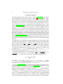
Although clingcon’s solving components follow the approach of modern SMT solvers
when combining the ASP solver clasp with the CP solver gecode, clingcon furthermore
adheres to the tradition of ASP in supporting a corresponding modeling language based
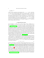
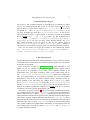
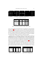
on the ASP grounder gringo. The resulting tripartite architecture of clingcon is depicted in
Figure 1. Although in the current implementation the theory solver is instantiated with the
CP solver gecode, the principal design of clingcon along with the corresponding interfaces
are conceived in a generic way, aiming at arbitrary theory solvers.
Following the workflow in Figure 1, the first extension concerns the input language of
gringo with theory-specific language constructs. Just as with regular atoms, the grounding
capabilities of gringo can be used for dealing with constraint atoms containing first-order
variables. As regards the current clingcon system, the language extensions allow for expressing constraints over integer variables. As we detail in Section 4, this involves arithmetic constraints as well as global constraints and optimization statements. These constraints are treated as atoms and passed to clasp via the standard gringo-clasp interface,
also used in clingo, the monolithic combination of gringo and clasp. Information about
these constraints is furthermore directly shared with the theory propagator and in turn the
theory solver, viz. gecode. In the new version of clingcon, the theory propagator is implemented as a post propagator, as furnished by clasp.1 Theory propagation is done in the
theory solver until a fixpoint is reached. In doing so, decided constraint atoms are transferred to the theory solver, and conversely constraints whose truth values are determined
by the theory solver are sent back to clasp using a corresponding nogood. Note that theory
propagation is not only invoked when propagating partial assignments but also whenever
a total Boolean assignment is found. Whenever the theory solver detects a conflict, the
theory propagator is in charge of conflict analysis. Apart from reverting the state of the
theory solver upon backjumping, this involves the crucial task of determining a conflict
nogood (which is usually not provided by theory solvers, as in the case of gecode). This is
elaborated upon in Section 5. Similarly, the theory propagator is in charge of enumerating
constraint variable assignments, whenever needed. Finally, we note that the theory propagator is informed whenever constraint atoms are decided. This allows for updating watches
1
Post propagators provide an abstraction easing clasp’s extensibility with more elaborate propagation mechanisms. To this end, clasp maintains a list of post propagators that are consecutively processed after unit propagation. Also, lookahead and unfounded-set checking are implemented in clasp as post propagators.
4
Max Ostrowski and Torsten Schaub
Listing 1: Example of a constraint logic program
1
2
3
4
$domain(0..10).
person(adam;smith;lea;john).
1{team(A,B) : person(B) : B != A}1 :- person(A), A == adam.
{friday}.
6
7
8
9
work(A) $+ work(B) $> 6 :- team(A,B).
work(B) $- work(adam) $== 1 :- friday, team(adam,B).
:- team(adam,lea), not work(lea) $== work(adam).
work(B) $== 0 :- person(B), not team(adam,B), B != adam.
11
$count[work(A) $== 8 : person(A)] $== fulltime.
13
$maximize{work(A) : person(A)}.
for constraint literals, even before propagation is launched. This is implemented by clasp’s
call-back routines, another new feature of clasp supporting theory solving.
4 The clingcon Language
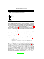
We explain the syntax of our constraint logic programs via the example in Listing 1.
Suppose Adam wants to do house renovation with the help of three friends. We encode
the problem as follows. In Line 1 we restrict all constraint variables to the domain [0, 10]
as nobody wants to work more than 10 hours a day. In Line 3 we choose teams. They
agreed that each team has to work more than six hours a day (Line 6). Within this line we
show the syntax of linear constraints. They can be used in the head or body of a rule2 . We
use the $ sign in front of every relation and function symbol referring to the underlying
CSP. In this new clingcon version this also applies to arithmetic operators to better separate them from gringo operators. Many standard arithmetical operators are supported, like
plus(+), times(∗) and absolute(abs). We use the grounding capabilities of gringo to create
the constraint variables. Grounding Line 6 yields:
work(adam) $+ work(smith) $> 6 :- team(adam,smith).
work(adam) $+ work(lea)
$> 6 :- team(adam,lea).
work(adam) $+ work(john) $> 6 :- team(adam,john).
We created three ground rules containing three different constraints, using four different
constraint variables. Note that the constraint variables have not been defined beforehand.
All variables occurring in a constraint are automatically constraint variables. On Fridays,
Adam has to pick up his daughter from sports and therefore works one hour less than his
partner (Line 7). Furthermore Lea and Adam are a couple and decided to have an equal
work load if they are in the same team (Line 8). Finally, Line 9 prevents persons from
working if they are not teammates.
With this little constraint logic program, we want to show how for example quantities can be easily expressed. Constraints and constraint variables fit naturally into the logic
program. Not representing quantities explicitly with propositional variables eases the modelling of problems and also decreases the size of the ground logic program.
Global Constraints. In Line 11 we use a global constraint. This is a new feature of
clingcon. Global constraints capture relations between a non-fixed number of variables. As
2
Constraint atoms in the head are shifted to the negative body.
ASP modulo CSP: The clingcon system
5
with aggregates in gringo, we can use conditional literals (Syrjänen ) to represent these
sets of variables. In the example we can see a count constraint. Grounding this yields:
$count[work(adam) $== 8, work(smith) $== 8,
work(lea) $== 8, work(john) $== 8] $== fulltime.
It constrains the number of variables in {work(adam), work(smith), work(lea),
work(john)} that are equal to 8, to be equal to fulltime. Constraint variable
fulltime counts how many persons are working full time. Global constraints do have a
similar syntax to propositional aggregates. Also their semantics is similar to count aggregates in ASP (cf. (Schulte et al. 2012)). But global constraints only constrain the values of
constraint variables, not propositional ones.
Clingcon also supports the global constraint distinct, where
$distinct{work(A) : person(A)}.
means that all persons should have a different workload. That is, all values assigned to constraint variables in {work(adam), work(smith), work(lea), work(john)} have
to be distinct from each other. This constraint could also be expressed using a quadratic
number of inequalities. Using a single dedicated constraint is usually much more efficient
in terms of memory consumption and runtime.
As global constraints are usually not supported in a negated form in a CP solver, we have
the syntactic restriction that all global constraints must become facts during grounding and
therefore may only occur in the head of rules. Further global constraints can easily be
integrated into this generic framework.
A valid solution to our constraint logic program in Listing 1 contains the regular
literal Tteam(adam,smith), but also constraint literals like Twork(lea)$==0,
Twork(john)$==0 and Twork(adam)$+work(smith)$>6. The solution also
contains assignments to constraint variables, like work(adam)7→8, work(smith)7→3,
work(lea)7→0, work(john)7→0 and fulltime7→1.
Optimization. In Line 13 we give a maximize statement over constraint variables. This is also a new feature of clingcon. We maximize the sum over a set
of variables and/or expressions. In this case, we try to maximize work(adam) $+
work(smith) $+ work(lea) $+ work(john). For optimization statements
over constraint variables, we also rely on the syntax of gringo’s propositional optimization statements. We support minimization/maximization and multi-level optimization. To distinguish propositional and constraint statements, we precede the latter with a $ sign. One optimal solution to the problem contains the propositional literal Tteam(adam,john), and the constraint literals Twork(lea)$==0,
Twork(smith)$==0, and Twork(adam)$+work(john)$>6. To maximize work
load, the constraint variables are assigned work(adam)7→10, work(smith)7→0,
work(lea)7→0, work(john)7→10 and fulltime7→0.
To find a constraint optimal solution, we have to combine the enumeration techniques
of clasp with the ones from the CP solver. Therefore, when we first encounter a full propositional assignment, we search for an optimal (w.r.t. to the optimize statement) assignment
of the constraint variables using the search engine of the CP solver. Let us explain this with
the following constraint logic program.
$domain(1..100).
6
Max Ostrowski and Torsten Schaub
a :- x $* x $< 25.
$minimize{x}.
Assume clasp has computed the full assignment {Fx $* x $< 25, Fa}. Afterwards,
we search for the constraint optimal solution to the constraint variable x which yields
{x 7→ 5}. Given this optimal assignment, a constraint can be added to the CP solver
that all further solutions shall be below/above this optimum (x$<5). This constraint will
now restrict all further solutions to be “better”. We enumerate further solutions, using the
enumeration techniques of clasp. So the next assignment is {Tx $* x $< 25, Ta} and
the CP solver finds the optimal constraint variable assignment {x 7→ 1}. Each new solution
restricts the set of further solutions, so our constraint is changed to (x$<1) which then
allows no further solutions to be found.
5 Conflict Filtering in clingcon
The development of Conflict Driven Clause Learning (CDCL) algorithms was a
major breakthrough in the area of SAT. Also, CDCL is crucial in SMT solving
(cf. (Nieuwenhuis et al. 2006)). A prerequisite to combine a CDCL-based SAT solver with
a theory solver is the possibility to generate good conflicts and reasons originating in the
underlying theory. Therefore, modern SMT solvers use their own specialized theory propagators that can produce such witnesses. Clingcon instead uses a black-box approach regarding theory solving. In fact, off-the-shelf CP solvers, like gecode, do usually not provide any
reason for their underlying inference. As a consequence, conflict and reason information
was so far only crudely approximated in clingcon. We address this shortcoming by developing mechanisms for extracting minimal reasons and conflicts from any CP solver using
monotone propagators. We assume that the reader has basic knowledge on CDCL-based
ASP solving, and direct the interested reader to (Gebser et al. 2007).
Whenever the CP solver finds out that the set of constraints is inconsistent under the
current assignment A, a conflicting nogood N must be generated, which can then be used
by the ASP solver in its conflict analysis. The simple version of generating the conflicting
nogood N , is just to take the entire assignment of constraint literals. In this way, all yet
decided constraint atoms constitute N = {ℓ | ℓ ∈ A|C }. In this case, the corresponding list
of inconsistent constraints is
I = [ γ(ℓ) | ℓ ∈ A|C ].
(1)
In order to reduce this list of inconsistent constraints and to find the real cause of the conflict, we apply an Irreducible Inconsistent Set (IIS) algorithm. The term IIS was coined
in (van Loon 1981) for describing inconsistent sets of constraints having consistent subsets only. We use the concept of an IIS to find the minimal cause of a conflict. With this
technique, it is actually possible to drastically reduce such exhaustive sets of inconsistent
constraints as in (1) and to create a much smaller conflict nogood. It is now possible to
apply an IIS algorithm to every conflicting set of constraints in order to provide clasp with
smaller nogoods. This enhances the information content of the learnt nogood and hopefully speeds up the search process by better pruning the search space. Clingcon now features several alternatives to reduce such conflicts. To this end, we build upon the approach
of (Chinneck and Dravinieks 1991) who propose different algorithms for computing IISs,
ASP modulo CSP: The clingcon system
7
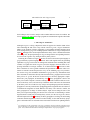
Algorithm 1: DELETION FILTERING
Input : An inconsistent list of constraints I = [c1 , . . . , cn ].
Output: An irreducible inconsistent list of constraints.
1
2
3
4
5
6
7
i←1
while i ≤ |I| do
if I \ ci is inconsistent then
I ← I \ ci
else
i←i+1
return I
among them the so-called Deletion Filtering algorithm. In what follows, we first present
the original idea of Deletion Filtering and afterwards propose several refinements that can
then be used to reduce inconsistent lists of constraints in the context of ASP modulo CSP.
Deletion Filtering. Given an inconsistent list of constraints I = [c1 , . . . , cn ] as in (1)
the Deletion Filtering Algorithm 1 reduces it to an irreducible list. We test for each ci ∈ I
whether I \ ci is inconsistent or not. If it is inconsistent we can restart the whole algorithm
with the list I \ ci continuing with the next i.
The result of this simple approach is a minimal inconsistent list, as we can see
in the following example. Suppose we branch on Tteam(adam,lea). Unit propagation implies the literals Twork(lea)$==work(adam), Twork(john)$==0,
Twork(smith)$==0, and Twork(adam)$+work(lea)$>6. At this point we cannot do any constraint propagation3 and make another choice, Tfriday, and some unit
propagation, resulting in Twork(lea)$-work(adam)$==1. As unit propagation is
at fixpoint, the CP solver checks the constraints in the partial assignment A|C for consistency. As it is inconsistent, a simple conflicting nogood would be N = {ℓ | ℓ ∈ A|C }. To
minimize this nogood, we now apply Deletion Filtering to the list I as defined in (1):
I = [γ(ℓ) | ℓ ∈ A|C ]
= [work(lea) = work(adam), work(john) = 0, work(smith) = 0]
◦ [work(adam) + work(lea) > 6, work(lea) − work(adam) = 1]
For i = 1, we test [work(john) = 0, work(smith) = 0, work(adam) + work(lea) >
6, work(lea) − work(adam) = 1], but it does not lead to inconsistency (Line 3). Next list
to test is [work(lea) = work(adam), work(smith) = 0, work(adam) + work(lea) >
6, work(lea) − work(adam) = 1] which restricts the domains of work(adam) and
work(lea) to ∅. As this is inconsistent, we remove work(john) = 0 from I and go on,
also removing work(smith) = 0 and work(adam) + work(lea) > 6. We end up with
the irreducible list I = [work(lea) = work(adam), work(lea) − work(adam) = 1],
and can now build a much smaller conflicting nogood N = {γ −1 (c) | c ∈ I} =
3
w.l.o.g. we assume arc consistency (Mohr and Henderson 1986)
8
Max Ostrowski and Torsten Schaub
Algorithm 2: FORWARD FILTERING
Input : An inconsistent list of constraints I = [c1 , . . . , cn ].
Output: An irreducible inconsistent list of constraints I ′ .
1
2
3
4
5
6
7
8
9
I ′ ← []
while I ′ is consistent do
T ← I′
i←1
while T is consistent do
T ← T ◦ ci
i←i+1
I ′ ← I ′ ◦ ci
return I ′
{Twork(lea)$==work(adam), Twork(lea)$-work(adam)$==1} as this really describes the cause of the inconsistency.
In most CP solvers, propagation is done in a constraint space. This space contains the
constraints and the variables of the problem. After doing propagation, the domains of the
variables are restricted. Normally in CP solvers like gecode this effect cannot be undone.
As long as we add further constraints to the constraint space this is no problem, as another
constraint restricts the domain of the variables even more. If we want to remove a constraint
from a constraint space we have to create a new space containing only the constraints we
want to apply. Then we have to redo all the propagation. This is why we identified Line 4
in Algorithm 1 as an efficiency bottleneck. To address this problem, we propose some
derivatives of the algorithm.
Forward Filtering. Algorithm 2 is designed to avoid resetting the search space of the CP
solver. It incrementally adds constraints to a testing list T , starting from the first assigned
constraint to the last one (lines 5 and 6). Remember that incrementally adding constraints
is easy for a CP solver as it can only further restrict the domains. If our test list T becomes
inconsistent we add the currently tested constraint to the result I ′ (lines 5 and 8). If this
result is inconsistent (Line 2), we have found a minimal list of inconsistent constraints.
Otherwise, we start again, this time adding all yet found constraints I ′ to our testing list T
(Line 1). Now we have to create a new constraint space. But by incrementally increasing
the testing list, we already reduced the number of potential candidates that contribute to the
IIS, as we never have to check a constraint beyond the last added constraint. We illustrate
this again on our example. We start Algorithm 2 with T = I ′ = [] and
I = [work(lea) = work(adam), work(john) = 0, work(smith) = 0]
◦ [work(adam) + work(lea) > 6, work(lea) − work(adam) = 1]
in Line 3. We add work(lea) = work(adam) to T , as this constraint alone is consistent, we loop and add constraints until T = I. As this list is inconsistent, we add the last
constraint work(lea) − work(adam) = 1 to I ′ in Line 8. We can do so, as we know
that the last constraint is indispensable for the inconsistency. As I ′ is consistent we restart
the whole procedure, but this time setting T = I ′ = [work(lea) − work(adam) = 1]
ASP modulo CSP: The clingcon system
9
Algorithm 3: RANGE FILTERING
Input : An inconsistent list of constraints I = [c1 , . . . , cn ].
Output: A (possibly smaller) inconsistent list of constraints I ′ .
5
I ′ ← []
i←n
while I ′ is consistent do
I ′ ← I ′ ◦ ci
i←i−1
6
return I ′
1
2
3
4
in Line 3. Please note that, even if I would contain further constraints, we would never
have to check a constraint behind work(lea) − work(adam) = 1. Our testing list
already contained an inconsistent set of constraints, consequently we can restrict ourself to this subset. Now we start the loop again, adding work(lea) = work(adam)
to T . On their own, these two constraints are inconsistent, as there exists no valid pair
of values for the variables. So we add work(lea) = work(adam) to I ′ , resulting in
I ′ = [work(lea) − work(adam) = 1, work(lea) = work(adam)]. This is then our
reduced list of constraints and the same IIS as we got with the Deletion Filtering method
(as it is the only IIS of the example). But this time we only needed one reset of the constraint space (Line 3) instead of five.
Backward Filtering. The basic idea of this algorithm is the same as in Algorithm 2. But
this time, we reverse the order of the inconsistent constraint list. Therefore, we first test
the last assigned constraint and iterate to the first. In this way we want to accommodate the
fact, that one of the literals that was decided on the current decision level has to be included
in the conflicting nogood. Otherwise we would have recognized the conflict before.
Range Filtering. This algorithm does not aim at computing an irreducible list of constraints, but tries to approximate a smaller one to find a nice tradeoff between reduction of
size and runtime of the algorithm. Therefore, as shown in Algorithm 3, we move through
the reversed list of constraints I and add constraints to the result I ′ until it becomes inconsistent. In our example we cannot reduce the inconsistent list anymore, as the first and the
last constraint is needed in the IIS.
Connected Components Filtering. Algorithm 4 tries to make use of the structure of the
constraints. Therefore, it does not go forward or backward through the list of constraints
but follows their used constraint variables. We start with initializing our result I ′ and the
test list T and set our set of observed constraint variables ω to the variables inside the last
assigned constraint of our list I (lines 2 to 4). Then we start our main loop, remembering
how many variables we have seen so far (Line 6). We go over our reversed list of constraints
I (Line 8). If we find a constraint that contains some of the already inspected variables
(Line 9), we add it to our testing list T and extend the set of already seen variables ω.
We then continue iterating until our testing list T becomes inconsistent (Line 13). In this
case we add the last tested constraint to our result list I ′ (Line 14). If this list is already
inconsistent (Line 5), we return a minimal list of constraints (Line 19). If not, we restart the
loop. But this time the set of already seen variables is restricted to the set of variables in the
10
Max Ostrowski and Torsten Schaub
Algorithm 4: CONNECTED COMPONENT FILTERING
Input : An inconsistent list of constraints I = [c1 , . . . , cn ].
Output: An irreducible inconsistent list of constraints I ′ .
1
2
3
4
5
6
7
8
9
10
11
12
13
14
15
16
17
18
19
if size(I) = 0 then return ∅
I ′ ← []
T ← []
ω ← vars(cn )
while I ′ is consistent do
count ← |ω|
i ← size(I)
while T is consistent and i ≥ 0 do
if ω ∩ vars(ci ) 6= ∅ then
T ← T ◦ ci
ω ← ω ∪ vars(ci )
i←i−1
if T is inconsistent then
I ′ ← I ′ ◦ ci
ω ← {y | y ∈ vars(x) where x in I ′ }
I ← remove(T, ci )
T ← I′
if count = |ω| then ω ← {y | y ∈ vars(x) where x in I}
return I ′
constraints in I ′ . Furthermore, we only iterate over the constraints from the test list (Line
16), as this possibly shorter list is also an inconsistent list of constraints. If at one point
we have not found any non tested constraint that has common variables with the tested
ones (this can be the case if the last constraint of our input list I is not contained in the
minimal list of constraints), we simply add all variables to ω in Line 18 so that we do not
miss any constraint in the next iteration. With this algorithm, we want to take account of
the internal structure of the constraints. For our example, this means we start with the last
constraint work(lea) − work(adam) = 1 and completely ignore work(john) = 0 and
work(smith) = 0 as their variables do not occur anywhere in the other constraints. We
end up with the same IIS as with Forward Filtering without checking all constraints that
do not have common variables with the constraints from the IIS.
Connected Components Range Filtering. This algorithm is a combination of the Connected Components Filtering and the Range Filtering algorithms. That is why it does
not compute an irreducible list of constraints. We move through the list I like in Algorithm 4 and once our test list T becomes inconsistent we simply return it. This shall
combine the advantages of using the structure of the constraints in the Connected Components Filtering and the simplicity of the Range Filtering. We ignore work(john) = 0 and
work(smith) = 0 and end up with I ′ = {work(lea)−work(adam) = 1, work(adam)+
work(lea) > 6, work(lea) = work(adam)}.
ASP modulo CSP: The clingcon system
11
6 Reason Filtering in clingcon
Up to now we only considered reducing an inconsistent list of constraints to reduce
the size of a conflicting nogood. But we can do even more. If the CP solver propagates the literal l, a simple reason nogood is N = {ℓ | ℓ ∈ A|C } ∪ {l}. If we have
for example A|C = {Twork(john)$==0,Twork(lea)-work(adam)$==1}, the
CP solver propagates the literal Fwork(lea)$==work(adam). To use the proposed algorithms to reduce a reason nogood we first have to create an inconsistent
list of constraints. As J = [γ(ℓ) | ℓ ∈ A|C ] implies γ(l), this inconsistent list is
I = J ◦ [γ(l)] = [work(john) = 0, work(lea) − work(adam) = 1, work(lea) =
work(adam)]. So we can now use these various filtering methods also to reduce reasons generated by the CP solver. In this case the reduced reason is
{Twork(lea)-work(adam)$==1, Twork(lea)$==work(adam)}. Smaller reasons reduce the size of conflicts even more, as they are constructed using unit resolution.
These two new features of clingcon are available via the command line parameters: --csp-reduce-conflict=X and --csp-reduce-reason=X where X =
{simple,forward,backward,range,cc,ccrange}.
7 The clingcon System
The new filtering methods enhance the learning capabilities of clingcon. However, the new
version also features Initial Lookahead, Optimization and Propagation Delay. We will now
present these in more detail.
Initial Lookahead. As shown in (Yu and Malik 2006), initial lookahead on constraints can be very helpful in the context of SMT. It makes implicit knowledge (stored in the propagators of the theory solver) explicitly available to the
propositional solver. Our Initial Lookahead, which can be enabled using the option --csp-initial-lookahead=<true/false>, is restricted to constraint literals. As a preprocessing step, all of them are separately set to true and constraint
propagation is done. In this way, binary relations between constraints become explicitly available to the ASP solver. For example, Twork(smith)$==0 implies
Fwork(smith)-work(adam)$==1 whereas Twork(lea)$==work(adam) implies Fwork(lea)-work(adam)$==1. These are then directly translated into a nogood. Or more formal: all constraints c implied by a constraint literal Tℓ w.r.t. the theory
are added to clasp as the respective binary nogood {Tℓ, γ −1 (c)}.
Optimization. As shown in Section 4, clingcon now supports optimization statements
over constraint variables. The option --csp-opt-val expects a comma-separated list of
values, similar to the clasp 1.3 option --opt-val. With this option a value for every constraint optimization statement can be given. The solver will then start the search using these
values. This is especially useful in combination with the option --csp-opt-all, that is
used to compute all models that are less or equal to the last found bound. It forms the logical
equivalent to the clasp 1.3 option --opt-all. To compute all constraint-optimal solutions, one first computes one optimal solution. Afterwards, given the optimum value, the
same encoding can be used with the options --csp-opt-val and --csp-opt-all
to compute all optimal solutions.
12
Max Ostrowski and Torsten Schaub
Propagation Delay. With Propagation Delay we have a new experimental feature that
balances the interplay between the ASP and the CSP part. Constraint propagation can
be expensive, especially in combination with the filtering techniques from Section 5. It
might be beneficial to give more attention to the ASP solver. This can be done by skipping constraint propagations. Whenever we can propagate a constraint atom or encounter
a conflict with the CP solver, filtering methods can be applied. If we therefore skip constraint propagation and only do it every n’th time, clasp has the chance to find more conflicts. If we learn less from the CSP side, we learn more from the ASP side. The option
--csp-prop-delay=n where n ∈ N+
0 can be used to set the propagation delay:
• n = 1 does constraint propagation every time, similar to the old clingcon,
• n > 1 does constraint propagation only every n’th time and
• n = 0 does constraint propagation only on a full propositional assignment.
Whenever we do constraint propagation we have to catch up on the missed propagation.
8 Experiments
We collected various benchmarks from different categories to evaluate the effects of our
new features on a broad range of problems. All of them can be expressed using a mixed
representation of Boolean and non-Boolean variables. We restrict ourself to classes where
the ASP and the CSP part interact tightly to solve the problem, as we focus on the learning
capabilities between the two systems. For encodings where we do not have an ASP or a
CSP part, we will not see any effect of our new features. We now present our benchmark
classes with a short description of the used encodings. All encodings and instances can be
found online at (clingcon).
Benchmarks. Given a set of squares, the Packing problem is to pack all squares into a
rectangular area with fixed dimension. This problem is directly taken from the 2011 ASP
Competition (ASP 2011). The position of the corners of the squares can be represented
using integer variables. and are guessed by the CP solver. Within ASP we only have to
check whether two squares overlap.
Incremental Scheduling is a problem variant of the well-known job shop scheduling
problem which requires rescheduling and ordering of jobs. Furthermore, all jobs have a
deadline, and, if a job finishes after its deadline, the difference is taken as “tardiness” of
the job. This tardiness multiplied by the importance of the job results in a penalty. The task
is to find a solution where the sum of all penalties is below a given maximum. The problem
is also taken from the 2011 ASP Competition. We use constraint variables to denote the
starting times of the jobs and also to compute the tardiness and penalties.
Taken from the 2011 ASP Competition, the Weighted Tree problem is inspired by costbased “join-order” optimization of SQL queries in databases. The problem is to find a full
binary tree with n leaves such that its leaves are pairs (weight, cardinality) of integers,
the right child of an inner node is a leaf, where its color is either green, red, or blue, and
there are 1, . . . , n − 1 inner nodes such that node n − 1 is a root node and inner node
i − 1 is the left child of inner node i for i = 2, . . . , n − 1. The weights of inner nodes
are computed recursively based on their colors, and the weights and cardinalities of their
children. We use constraint variables to represent the cardinality and the weight of the
ASP modulo CSP: The clingcon system
13
nodes. We furthermore extended the problem to an optimization problem that tries to find
the “cheapest” tree by minimizing the sum of the leaf weights according to the structure of
the tree. For this we use the new optimization statement over constraint variables. In our
benchmarks, an instance is solved if we have found and proven the optimal solution.
Given an n × n board, placing numbers in the range {1, . . . , n} such that there are
no two equal numbers in the same row/column is called Quasi Group problem. For our
benchmarks, we let n = 20. We assign random numbers to 0 − 80 percent of the fields.
To increase the spectrum of benchmarks, we conceived a new collection of benchmarks
which make use of the CP solver to do the Unfounded Set Check (USC) for some normal
logic programs. Therefore, we reify (Gebser et al. 2011; Gebser et al.) logic programs (in
our case we take Labyrinth – the problem of guiding an avatar through a dynamically
changing labyrinth to certain fields (ASP 2011), HashiwoKakero – a logic puzzle game
and HamiltonianCycle). Using this reified program we can reason about the structure of
the program. In particular, we can add an encoding that does the unfounded set check using
level-mapping as proposed in (Niemelä 2008). We assign a level to every atom in a strongly
connected component and use the CP solver to find a valid mapping. Using this translation,
we can solve any non-tight logic program using the CP solver for the unfounded set check.
Settings. We run our benchmarks single-threaded on a cluster with 24 × 8 cores with
2.27GHz each. We restricted each run to use 4GB RAM. In all our benchmarks we used
the standard configuration of clingcon, unless stated otherwise. We now evaluate the new
features of clingcon.
Global Constraints. We want to check whether the use of global constraints speeds up
the computation. Therefore we have chosen the Quasi Group problem, as it can be easily
expressed using the global constraint distinct. We compare two different encodings for
Quasi Group. The first one uses one distinct constraint for every row and every column. The
second one uses a cubic number of inequality constraints. We tested 78 randomly generated
instances of size 20 × 20. While the first encoding using the global constraints results in an
average runtime of 220 seconds and 18 timeouts over all instances, the decomposed version
was much slower. It used 391 seconds on average and had 27 timeouts. Clingcon confirms,
that global constraints are handled more efficiently than their explicit decomposition.
Initial Lookahead. In Section 7, we presented Initial Lookahead over constraints as a
new feature of clingcon. We now want to study in which cases this technique can be useful
in terms of runtime. We run all our benchmarks once with and without Initial Lookahead.
In Table 1, the first column shows the problem class and its number of instances. The second and the third column show the average runtime in seconds that is used with and without
Initial Lookahead (I.L.). Timeouts are shown in parenthesis. The last two columns show
the average runtime of the lookahead algorithm and the number of nogoods that have been
produced on average per instance. As we can see for the problems Packing, Quasi Group,
and Weighted Tree, direct relations between constraints can be detected and the overall runtime can therefore be reduced. But this technique does not work on all benchmark classes.
For Incremental Scheduling relations between constraints are found but the additional nogoods seem to deteriorate the performance of the solver. In the case of the Unfounded Set
Check, nearly no relations have been found, so no difference in runtime can be detected.
Conflict and Reason Filtering. We want to analyze how much the different conflict and
reason filtering methods presented in Section 5 differ in size of conflicts and average run-
14
Max Ostrowski and Torsten Schaub
instances
(#number)
Packing(50)
Inc. Sched.(50)
Quasi Group(78)
Weighted Tree(30)
USC(132)
time
(timeouts)
888(49)
30(01)
390(28)
484(07)
721(104)
time
with I.L
882(49)
40(02)
355(24)
312(04)
719(103)
time
of I.L.
5
0
9
0
3
nogoods
from I.L
7970
73
105367
1520
1
Table 1: Initial Lookahead (I.L.)
s
b
f
c
r
o
s
b
f
c
r
o
s
b
f
c
r
o
s
b
f
c
r
o
s
s
s
s
s
s
b
b
b
b
b
f
f
f
f
f
c
c
c
c
c
r
r
r
r
r
o
o
o
o
o
(a) Packing
(b) Inc. Shed.
(c) Quasi Group
(d) Weighted Tree
b
f
c
r
o
(e) USC
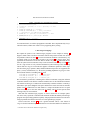
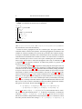
Fig. 2: Average conflict size
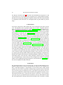
time. As conflicts and reasons are strongly interacting in the CDCL framework, we test the
combination of all our proposed algorithms. We denote the filtering algorithms with the
following shortcuts: s(Simple), b(Backward Filtering), f(Forward Filtering), c(Connected
Component Filtering), r(Range Filtering) and o(Connected Component Range Filtering).
We name the filtering algorithm for reasons first, separated by a slash from the algorithm
used to filter conflicts. To denote the configuration using Range Filtering for reasons and
Forward Filtering for conflicts, we simply write r/f. The original configuration, which can
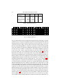
be seen as the “old” clingcon is therefore denoted s/s. We start by showing the impact
on average conflict size of all configurations using a heat map in Figure 2. It shows the
reduction of the conflict size in percentage relative to the worst configuration. The rows
represent the used algorithms for reason filtering, the columns represent the algorithms for
filtering conflicts. So the worst configuration is represented by a totally black square and a
configuration that reduces the average conflict size by half is gray. A completely white field
would mean that the conflict size has been reduced to zero. As we can see in Figure 2, the
average conflict size is reduced by all combinations of filtering algorithms. Furthermore,
we see that the first row and column, respectively, is usually darker than the others, which
indicates that filtering either only conflicts or only reasons is not enough. Also we see that
for the Unfounded Set Check (USC) the filtering of reasons does not have any effect. This
is due the encoding of the problem. As nearly no propagation takes place, no reasons are
computed at all. The shades on the Range Filtering rows/columns (denoted by r) clearly
show that the Range Filtering produces larger conflicts. But this is improved by incorporating structure to the filtering algorithm using Connected Component Range Filtering. Next,
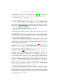
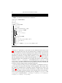
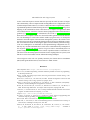
we want to see if the reduction of the average conflict size also pays off in terms of runtime.
Therefore Figure 3 shows the heat map for average runtime. A black square denotes the
slowest configuration, while a gray one is twice as fast. As we can clearly see, the reduction of runtime coincides with the reduction of conflict size in most cases. Furthermore, we
ASP modulo CSP: The clingcon system
s
b
f
c
r
o
s
b
f
c
r
o
s
b
f
c
o
r
s
b
f
15
c
r
o
s
s
s
s
s
s
b
b
b
b
b
f
f
f
f
f
c
c
c
c
c
r
r
r
r
r
o
o
o
o
o
(a) Packing
(b) Inc. Sched.
(c) Quasi Group
(d) Weighted Tree
b
f
c
r
o
(e) USC
Fig. 3: Average time in seconds
Instances
(#number)
Packing(50)
Inc. Sched.(50)
Quasi Group(78)
Weighted Tree(30)
USC(132)
time
s/s
888(49)
30(01)
390(28)
484(07)
721(104)
time
o/b
63(0)
3(0)
12(0)
574(18)
92(1)
acs
s/s
293
15
480
31
454
acs
o/b
40
5
56
31
13
Table 2: Average time in s(timeouts), average conflict size (acs)
can see a clear speedup for all benchmark classes except Weighted Tree using the filtering
algorithms. Table 2 compares the Simple version s/s without using any filtering algorithms,
with the configuration o/b (reducing reasons using Connected Component Range Filtering
and reducing conflicts using Backward Filtering), as it has the lowest number of timeouts.
We can see a speedup of around one order of magnitude on all benchmarks except Weighted
Tree. The same picture is given for the reduction of conflict size. So whenever it is possible
to reduce the average conflict size, this also pays off in terms of runtime.
Propagation Delay. As the filtering of conflicts and reasons takes a lot of time (e.g
configuration o/b uses 43% of the runtime for filtering), we want to reduce the calls to the
filtering algorithms. Therefore, with Propagation Delay, we can do less propagation with
the CP solver and it will produce less conflicts and reasons, hopefully reducing the number
of calls. We therefore take the yet best configuration o/b and compare different propagation
delays n ∈ {1, 10, 0} (normal, every ten steps, only on model). Table 3 shows the average
number of calls to a filtering algorithm for configuration o/b with different delays. We see
a reduction of the number of calls on all benchmarks except on Incremental Scheduling
where it doubled. This is clearly due to a loss of information that is necessary for the
search. If the CP solver has less influence on the search, the ASP part gets more control.
But the missing knowledge from the CSP part has to be compensated by pure search in
n
Packing
Inc. Sched.
Quasi Group
Weighted Tree
USC
1
31534
3505
4245
6868k
2007
10
14897
3240
1535
1168k
2118
0
8463
6660
1726
1042k
1768
Table 3: Calls to filtering algorithms o/b
n
Packing
Inc. Sched.
Quasi Group
Weighted Tree
USC
1
63
3
12
574
92
10
75
6
9
559
91
0
571
11
19
546
82
Table 4: Times of configuration o/b
16
Max Ostrowski and Torsten Schaub
the ASP part. Therefore, Table 4 shows that some benchmarks like Weighted Tree and
Unfounded Set Check can relinquish some propagation power gaining additional speedup.
On others like Packing this propagation is urgently needed to drive the search and cannot
be compensated. This feature has to be investigated further to gain benefits for practical
usage.
9 Related Work
In the quite young field of ASP modulo CSP a lot of research has been done in the last
years. The approaches can be separated roughly into two classes: integration and translation. The integrated approaches like CASP (Baselice et al. 2005) and ADSolver/ACSolver (Mellarkod and Gelfond 2008; Mellarkod et al. 2008) are similar to the clingcon
system. However, no learning is used in the approaches, as the constraint solver just checks
the assignment of constraints. Later, (Balduccini 2009) showed how to use ASP as a specification language, where each answer set represents a CSP. In this approach no coupling
between the systems was possible and therefore learning facilities were not used. Afterwards GASP (Dal Palù et al. 2009) presented a bottom up approach where the logic program was grounded on the fly. With Dingo (Janhunen et al. 2011) ASP was translated to
difference logic using level mapping for the unfounded set check. An SMT solver is used
to solve the translated problem. Nowadays, more and more translational approaches arise
in the area of SMT. Sugar (Tamura et al. 2008) is a very successful solver which translates
the various supported theories to SAT. Also, in (Drescher and Walsh 2010) it was shown
how to translate constraints into ASP during solving. These translational approaches have
the strongest coupling and therefore the highest learning capabilities. The reason generation and conflict handling is directly done by the underlying SAT solver and therefore
very efficient. On the other hand, they do have problems to find a compact representation
of the constraints without losing propagation strength. Clingcon therefore tries to catch
up, improving the learning facilities and still preserving the advantages of integrated approaches like compact representation of constraint propagators. Furthermore, clingcon is a
ASP modulo Theory solver that aims at taking advantage of arbitrary theories in the long
run, eg description logics. Such a variety can only be supported by a black box approach.
Similar results regarding the filtering methods have been introduced in (Junker 2001) but
have not been applied to an SMT framework.
10 Discussion
We extended and improve clingcon in various ways. At first, the input language was expanded to support Global Constraints and Optimization Statements over constraint variables. As the input language is a big advantage over pure SMT systems, complex hybrid
problems can now easily be expressed as constraint logic programs. We have shown that
Initial Lookahead can give advantages in terms of speedup on some problems. We developed Filtering methods for conflicts and reasons that can be applied to any theory solver.
This enables the ASP solver to learn about the structure of the theory, even if the theory
solver does not give any information about it (black box systems). We furthermore show
that while applying these filtering methods, that knowledge is discovered that is valuable
ASP modulo CSP: The clingcon system
17
for the overall search process and can therefore speed up the search by orders of magnitude. Unfortunately, a direct comparison with existing SMT solvers is inapplicable in view
of different input formats. However, we want to conduct an indirect comparison by translating ASPmCSP problems to SMT following the line of (Janhunen et al. 2011), using a level
mapping for the unfounded set check. This allows us to compare our approach to SMT
solvers that do not use a black-box CP solver but do propagation either with dedicated algorithms (eg. (Bofill et al. 2008)) or a translation of CP to SAT (cf. (Tamura et al. 2008)).
Such solvers have complete control over reason and conflict generation and can therefore
use extra knowledge to create better conflicts. With Propagation Delay we developed a
method to control the impact of the interaction among both systems to the search. To balance the Propagation Delay dynamically during search will be topic of additional research.
Our work leaves the burden of choosing the right reason and conflict generation strategy
to the user. Although for our benchmark set the optimal filtering configuration was o/b,
this may vary on other benchmark classes. This can be counterbalanced by an adaption of
the claspfolio (Gebser et al. 2011) system to clingcon in order to automatically derive an
optimal configuration of clingcon from the features of problem instances. In the future we
still want to focus on learning capacities and increase the coupling of the two systems, such
that the CP solver also benefits from the elaborated learning techniques.
Acknowledgments This work was partially funded by the German Science Foundation
(DFG) under grants SCHA 550/8-2, SCHA 550/10-1 AOBJ: 593494.
References
ASP Competition. 2011. https://www.mat.unical.it/aspcomp2011/.
BALDUCCINI , M. 2009. Representing constraint satisfaction problems in answer set programming.
In Workshop ASPOCP’09.
BARAL , C. 2003. Knowledge Representation, Reasoning and Declarative Problem Solving. Cambridge University Press.
BASELICE , S., B ONATTI , P., AND G ELFOND , M. 2005. Towards an integration of answer set and
constraint solving. In Proceedings of ICLP’05, Springer, 52–66.
B IERE , A., H EULE , M., VAN M AAREN , H., AND WALSH , T., 2009. Handbook of Satisfiability.
Frontiers in Artificial Intelligence and Applications. IOS Press.
B OFILL , M., N IEUWENHUIS , R., O LIVERAS , A., RODR ÍGUEZ -C ARBONELL , E., AND RUBIO , A.
2008. The barcelogic SMT solver. In Computer Aided Verification, Springer, 294–298.
C HINNECK , J. AND D RAVINIEKS , E. 1991. Locating minimal infeasible constraints sets in linear
programs. In ORSA Journal On Computing. 3, 157–168.
clingcon. http://www.cs.uni-potsdam.de/clingcon.
DAL PAL Ù , A., D OVIER , A., P ONTELLI , E., AND ROSSI , G. 2009. Answer set programming with
constraints using lazy grounding. See Hill and Warren (2009), 115–129.
D ECHTER , R. 2003. Constraint Processing. Morgan Kaufmann Publishers.
D RESCHER , C. AND WALSH , T. 2010. A translational approach to constraint answer set solving. In
TPLP. 10(4-6). Cambridge University Press, 465–480.
G EBSER , M., K AMINSKI , R., K AUFMANN , B., O STROWSKI , M., S CHAUB , T., AND T HIELE ,
S.
A user’s guide to gringo, clasp, clingo, and iclingo.
Available at
http://potassco.sourceforge.net.
18
Max Ostrowski and Torsten Schaub
G EBSER , M., K AMINSKI , R., K AUFMANN , B., S CHAUB , T., S CHNEIDER , M., AND Z ILLER , S.
2011. A portfolio solver for answer set programming: Preliminary report. In Proceedings of
LPNMR’11, Springer, 352–357.
G EBSER , M., K AMINSKI , R., AND S CHAUB , T. 2011. Complex optimization in answer set programming: Extended version. Unpublished draft. Available at (metasp).
G EBSER , M., K AUFMANN , B., N EUMANN , A., AND S CHAUB , T. 2007. Conflict-driven answer set
solving. In Proceedings of IJCAI’07, AAAI Press/The MIT Press, 386–392.
G EBSER , M., O STROWSKI , M., AND S CHAUB , T. 2009. Constraint answer set solving. See
Hill and Warren (2009), 235–249.
gecode. http://www.gecode.org.
G ELFOND , M. AND L IFSCHITZ , V. 1991. Classical negation in logic programs and disjunctive
databases. New Generation Computing 9, 365–385.
H ILL , P. AND WARREN , D., Eds. 2009. Proceedings of ICLP’09. Springer.
JANHUNEN , T., L IU , G., AND N IEMEL Ä , I. 2011. Tight integration of non-ground answer set
programming and satisfiability modulo theories. In Proceedings of GTTV’11, 1–13.
J UNKER , U. 2001. QuickXPlain: Conflict detection for arbitrary constraint propagation algorithms.
IJCAI’01 Workshop on Modelling and Solving problems with constraints.
M ELLARKOD , V. AND G ELFOND , M. 2008. Integrating answer set reasoning with constraint solving
techniques. In Proceedings of FLOPS’08, Springer, 15–31.
M ELLARKOD , V., G ELFOND , M., AND Z HANG , Y. 2008. Integrating answer set programming and
constraint logic programming. Annals of Mathematics and Artificial Intelligence 53, 1-4, 251–287.
metasp. http://www.cs.uni-potsdam.de/metasp.
M OHR , R. AND H ENDERSON , T. 1986. Arc and path consistency revisited. Artificial Intelligence 28, 2, 225–233.
N IEMEL Ä , I. 2008. Stable models and difference logic. Annals of Mathematics and Artificial Intelligence 53, 1-4, 313–329.
N IEUWENHUIS , R., O LIVERAS , A., AND T INELLI , C. 2006. Solving SAT and SMT: From an
abstract Davis-Putnam-Logemann-Loveland procedure to DPLL(T). JACM 53, 6, 937–977.
S CHULTE , C., TACK , G., AND L AGERKVIST, M. 2012. Modeling. In Modeling and Programming
with Gecode, C. Schulte, G. Tack, and M. Lagerkvist. Corresponds to Gecode 3.7.2.
S YRJ ÄNEN , T. Lparse 1.0 user’s manual. http://www.tcs.hut.fi/Software/smodels/lparse.ps.gz.
TAMURA , N., TANJO , T., AND BANBARA , M. 2008. System description of a SAT-based CSP solver
Sugar. In Third International CSP Solver Competition. 71–75.
VAN L OON , J. 1981. Irreducibly inconsistent systems of linear inequalities. In European Journal of
Operational Research. 3. Elsevier Science, 283–288.
Y U , Y. AND M ALIK , S. 2006. Lemma learning in SMT on linear constraints. In Theory and
Applications of Satisfiability Testing - SAT 2006, Springer, 142–155.