Download Desmond User Manual

Desmond User Manual
Desmond 2.2
User Manual
Schrödinger Press
Desmond User Manual Copyright © 2009 Schrödinger, LLC. All rights reserved.
While care has been taken in the preparation of this publication, Schrödinger
assumes no responsibility for errors or omissions, or for damages resulting from
the use of the information contained herein.
Canvas, CombiGlide, ConfGen, Epik, Glide, Impact, Jaguar, Liaison, LigPrep,
Maestro, Phase, Prime, PrimeX, QikProp, QikFit, QikSim, QSite, SiteMap, Strike, and
WaterMap are trademarks of Schrödinger, LLC. Schrödinger and MacroModel are
registered trademarks of Schrödinger, LLC. MCPRO is a trademark of William L.
Jorgensen. Desmond is a trademark of D. E. Shaw Research. Desmond is used with
the permission of D. E. Shaw Research. All rights reserved. This publication may
contain the trademarks of other companies.
Schrödinger software includes software and libraries provided by third parties. For
details of the copyrights, and terms and conditions associated with such included
third party software, see the Legal Notices for Third-Party Software in your product
installation at $SCHRODINGER/docs/html/third_party_legal.html (Linux OS) or
%SCHRODINGER%\docs\html\third_party_legal.html (Windows OS).
This publication may refer to other third party software not included in or with
Schrödinger software ("such other third party software"), and provide links to third
party Web sites ("linked sites"). References to such other third party software or
linked sites do not constitute an endorsement by Schrödinger, LLC. Use of such
other third party software and linked sites may be subject to third party license
agreements and fees. Schrödinger, LLC and its affiliates have no responsibility or
liability, directly or indirectly, for such other third party software and linked sites,
or for damage resulting from the use thereof. Any warranties that we make
regarding Schrödinger products and services do not apply to such other third party
software or linked sites, or to the interaction between, or interoperability of,
Schrödinger products and services and such other third party software.
Revision A, October 2009
Contents
Document Conventions ..................................................................................................... ix
Chapter 1: Introduction ....................................................................................................... 1
1.1 Installation and Configuration ................................................................................ 2
1.2 The Maestro Interface to Desmond ........................................................................ 3
1.3 Desmond Calculations Overview ........................................................................... 4
1.4 Citing Desmond in Publications ............................................................................. 5
Chapter 2: Building a Model System ........................................................................ 7
2.1 Adding Solvent .......................................................................................................... 7
2.2 Setting Up the Boundary Box ................................................................................. 8
2.3 Adding a Membrane .................................................................................................. 9
2.4 Using Custom Charges .......................................................................................... 11
2.5 Adding Ions .............................................................................................................. 11
2.5.1 Defining an Excluded Region............................................................................ 12
2.5.2 Ion Placement ................................................................................................... 12
2.5.3 Adding a Salt..................................................................................................... 14
2.6 Running the Job ...................................................................................................... 14
2.7 Quick Setup Instructions ....................................................................................... 14
Chapter 3: Running a Desmond Simulation from Maestro ...................... 17
3.1 Overview of the General Desmond Panels ......................................................... 17
3.2 Selecting a Model System ..................................................................................... 18
3.3 Minimizations ........................................................................................................... 19
3.4 Molecular Dynamics Simulations ......................................................................... 20
3.5 Simulated Annealing Simulations ........................................................................ 22
3.6 Replica Exchange Simulations ............................................................................. 24
3.7 Simulations on Systems with Membranes ......................................................... 26
Desmond 2.2 User Manual
iii
Contents
3.8 Setting Options for Desmond Simulations ......................................................... 27
3.8.1 The Integration Tab ........................................................................................... 28
3.8.2 The Ensemble Tab ............................................................................................ 29
3.8.3 The Minimization Tab ........................................................................................ 31
3.8.4 The Interaction Tab ........................................................................................... 32
3.8.5 The Restraints Tab............................................................................................ 33
3.8.6 The Output Tab ................................................................................................. 33
3.8.7 The Misc Tab..................................................................................................... 35
3.9 Running a Simulation Job ..................................................................................... 36
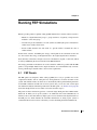
Chapter 4: Running FEP Simulations .................................................................... 39
4.1 FEP Panels................................................................................................................ 39
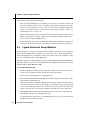
4.2 Ligand Functional Group Mutation ...................................................................... 40
4.3 Ring Atom Mutation ................................................................................................ 42
4.4 Protein Residue Mutation ...................................................................................... 44
4.5 Total Solvation Free Energy Calculation ............................................................. 46
4.6 Selecting the Environment and FEP Protocol .................................................... 47
4.7 FEP Results .............................................................................................................. 49
4.7.1 Relative Free-Energy Differences ..................................................................... 49
4.7.2 Total Solvation Free Energies ........................................................................... 49
4.8 Customizing and Restarting FEP Simulations .................................................. 50
Chapter 5: Analyzing Simulations ............................................................................. 53
5.1 Viewing Trajectories ............................................................................................... 53
5.2 Simulation Quality Analysis .................................................................................. 56
iv
Desmond 2.2 User Manual
Contents
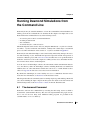
Chapter 6: Running Desmond Simulations from the Command
Line ......................................................................................................................................... 59
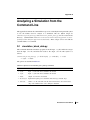
6.1 The desmond Command ........................................................................................ 59
6.2 Running Multiple Simulations ............................................................................... 62
6.2.1 Examples of Running MultiSim ......................................................................... 64
6.2.2 Sample MultiSim Job (.msj) File ....................................................................... 64
6.2.3 Treatment of Intermediate Files ........................................................................ 67
6.3 Building a Model System ....................................................................................... 67
6.3.1 Reading the Structures .................................................................................... 68
6.3.2 Adding a Membrane......................................................................................... 70
6.3.3 Setting the Box Shape and Dimensions............................................................ 70
6.3.4 Setting Force Field Information ......................................................................... 71
6.3.5 Setting the Number and Location of Ions.......................................................... 71
6.3.6 Solvating the System ....................................................................................... 72
6.3.7 Writing the Output File ...................................................................................... 72
Chapter 7: Using VMD for Desmond Trajectories .......................................... 73
7.1 Reading a CMS File and a Desmond Trajectory ............................................... 73
7.2 Writing a Maestro File ............................................................................................. 74
Chapter 8: Using Alternate Force Field Parameters and
Constraints......................................................................................................................... 77
8.1 The viparr Utility ...................................................................................................... 77
8.2 The build_constraints Utility ................................................................................. 79
8.3 Input and Output Files ............................................................................................ 80
8.4 Specifying Multiple Force Fields .......................................................................... 81
8.5 User-Defined Force Fields ..................................................................................... 82
8.6 Known Issues ........................................................................................................... 83
Desmond 2.2 User Manual
v
Contents
Chapter 9: Utilities................................................................................................................ 85
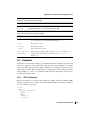
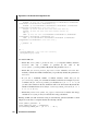
9.1 solvate_pocket ......................................................................................................... 85
9.1.1 Methodology ..................................................................................................... 85
9.1.2 Command Syntax ............................................................................................. 86
9.1.3 Command File Syntax....................................................................................... 86
9.2 manipulate_trj.py ..................................................................................................... 89
9.3 amber_prm2cms.py ................................................................................................ 90
9.4 mold_gpcr_membrane.py ...................................................................................... 90
9.5 forceconfig.py .......................................................................................................... 91
Appendix A: Creating a CMS File from a Full System Maestro File . 93
Appendix B: The multisim Utility................................................................................. 95
B.1 Running multisim .................................................................................................. 95
B.1.1 Template multisim Commands.......................................................................... 95
B.1.2 Node Locking.................................................................................................... 96
B.1.3 Restarting multisim Jobs .................................................................................. 96
B.1.4 Obtaining Information from multisim Checkpoint Files ..................................... 97
B.2 The multisim File Syntax ...................................................................................... 98
B.2.1 General Keywords .......................................................................................... 100
B.2.2 Desmond-Specific Common Keywords .......................................................... 100
B.2.3 The restrain Keyword...................................................................................... 101
B.2.4 The atom_group Keyword............................................................................... 102
B.2.5 The task Stage ............................................................................................... 103
B.2.6 The system_builder Stage .............................................................................. 103
B.2.7 The simulate and replica_exchange Stages................................................... 104
B.2.8 The minimize Stage ........................................................................................ 105
B.2.9 The solvate_pocket Stage .............................................................................. 106
B.2.10 The extern Stage .......................................................................................... 107
B.2.11 The fep_analysis Stage ................................................................................ 109
vi
Desmond 2.2 User Manual
Contents
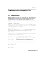
Appendix C: The Desmond Configuration File .............................................. 111
C.1 General Structure ................................................................................................ 111
C.2 Units ....................................................................................................................... 112
C.3 Configuration File Sections ............................................................................... 112
C.3.1 The boot Section ............................................................................................ 113
C.3.2 The constraint Section.................................................................................... 113
C.3.3 The Desmond Section .................................................................................... 113
C.3.4 The force Section ........................................................................................... 114
C.3.5 The global_cell Section .................................................................................. 116
C.3.6 The integrator Section .................................................................................... 117
C.3.7 The mdsim Section......................................................................................... 120
C.3.8 The minimize Section ..................................................................................... 121
C.3.9 The remd Section ........................................................................................... 121
C.3.10 The vrun Section .......................................................................................... 122
C.4 Plugin Descriptions ............................................................................................. 122
C.5 Examples ............................................................................................................... 125
C.5.1 FEP Calculations ............................................................................................ 125
C.5.2 Replica Exchange........................................................................................... 127
C.5.3 Simulated Annealing....................................................................................... 127
C.5.4 Instructing Desmond to Glue Close Solute Molecules Together .................... 127
Appendix D: Analyzing a Simulation from the Command Line ........... 129
D.1 simulation_block_data.py ................................................................................. 129
D.2 simulation_block_test.py .................................................................................. 130
D.3 Simulation Block Analysis (.sba) File Syntax ................................................. 130
D.4 Simulation Block Test (.sbt) File Syntax .......................................................... 131
References .............................................................................................................................. 133
Getting Help ........................................................................................................................... 137
Desmond 2.2 User Manual
vii
viii
Desmond 2.2 User Manual
Document Conventions
In addition to the use of italics for names of documents, the font conventions that are used in
this document are summarized in the table below.
Font
Example
Use
Sans serif
Project Table
Names of GUI features, such as panels, menus,
menu items, buttons, and labels
Monospace
$SCHRODINGER/maestro
File names, directory names, commands, environment variables, and screen output
Italic
filename
Text that the user must replace with a value
Sans serif
uppercase
CTRL+H
Keyboard keys
Links to other locations in the current document or to other PDF documents are colored like
this: Document Conventions.
In descriptions of command syntax, the following UNIX conventions are used: braces { }
enclose a choice of required items, square brackets [ ] enclose optional items, and the bar
symbol | separates items in a list from which one item must be chosen. Lines of command
syntax that wrap should be interpreted as a single command.
File name, path, and environment variable syntax is generally given with the UNIX conventions. To obtain the Windows conventions, replace the forward slash / with the backslash \ in
path or directory names, and replace the $ at the beginning of an environment variable with a
% at each end. For example, $SCHRODINGER/maestro becomes %SCHRODINGER%\maestro.
In this document, to type text means to type the required text in the specified location, and to
enter text means to type the required text, then press the ENTER key.
References to literature sources are given in square brackets, like this: [10].
Desmond 2.2 User Manual
ix
x
Desmond 2.2 User Manual
Desmond User Manual
Chapter 1
Chapter 1:
Introduction
Desmond is a new explicit-solvent molecular dynamics program developed by D. E. Shaw
Research. Desmond was created from scratch with an emphasis on accuracy, speed and scalability. It supports many of the most sought-after features in a modern molecular dynamics
program, including:
• Highly scalable parallel execution
• Explicit solvent simulations with periodic boundary conditions using cubic, orthorhombic, and triclinic simulation boxes. Truncated octahedron and rhombic dodecahedron are
supported via their triclinic analogues.
• Support for isotropic, semi-isotropic and anisotropic pressure coupling
• Smooth particle mesh Ewald method for accurate and efficient evaluation of long-range
electrostatics
• NVE, NVT, NPT, NPAT, NPγT ensembles with Berendsen, Langevin, or Nosé-Hoover
thermostats, and Berendsen, Langevin, or Martyna-Tobias-Klein barostats
• Symplectic integration of the equations of motion using a multiple time step approach,
RESPA
• Elimination of many sources of numerical error, permitting accurate and fast calculations
using single-precision arithmetic
• Accurate implementation of constraints to eliminate high-frequency motions and thus
permit larger time steps
• Exploitation of modern computer chip features to enhance speed (SIMD)
• Efficient calculation of the pressure
• Accurate checkpointing mechanism for continuing or restoring simulations
• Template-based support for widely-used force fields (using viparr).
• Viewing of trajectories with VMD using a Desmond plug-in.
A description of Desmond was published, along with performance data, as part of the conference proceedings of the ACM/IEEE Conference on SuperComputing 2006 (SC06) [1]. While
developing Desmond, D. E. Shaw Research has introduced and extended a number of scientific
Desmond 2.2 User Manual
1
Chapter 1: Introduction
algorithms, including new parallelization strategies and numerical techniques, some of which
have been published [2–5].
Problem-solving often involves using a wide range of modelling techniques, so integrating
Desmond into Schrödinger’s premier molecular modelling suite for drug development
enhances the utility of both. Examples of such synergies include:
• The Protein Preparation Wizard, LigPrep (ligand structure) and Epik (ligand protonation
state) preparation tools can be used to ensure that the structures provided to Desmond are
chemically correct. Such careful system preparation often represents a crucial step prior
to initiating a molecular dynamics simulation.
• Prime can be used to create homology models for use in simulations and to repair protein
structures.
• Glide can be used to generate relevant poses within protein binding sites for use in simulations. Desmond in turn can be used to thermally relax, refine, and sample conformations related to the docked poses.
• Strike can be used to generate statistical models from the results of simulations.
• Desmond can be used to sample protein structures prior to performing docking calculations with Glide.
• SiteMap can be used to identify potential binding sites from simulation results.
• WaterMap analyses specially designed Desmond simulations to characterize the thermodynamics of water in protein binding sites.
1.1
Installation and Configuration
Desmond is supported on x86 hardware under Linux, and is available in both 32-bit and 64-bit
versions. Detailed requirements and installation and configuration instructions are given in the
Installation Guide.
Although Desmond can run serially, for most purposes, you will want to make use of the
parallel execution capabilities. Desmond uses Open MPI for parallel execution. Before you can
run jobs, however, you must add entries to the hosts file for parallel execution with Open MPI,
in addition to any configuration that is needed for the hosts and the queueing system. See the
Installation Guide for instructions, especially Chapter 6 and Section 6.3.3.
2
Desmond 2.2 User Manual
Chapter 1: Introduction
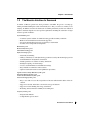
1.2
The Maestro Interface to Desmond
A number of Maestro panels have been provided to streamline the process of setting up,
running and understanding the results of Desmond jobs so that you can focus on what you are
studying. In addition, much of the framework for running Desmond jobs has been written in
Python to facilitate adaptation to user-specific requirements, including the automation of larger
and more specific workflows.
System Builder panel
•
•
•
•
Constructs systems suitable for simulation using periodic boundary conditions
Bulk solvent and membrane environments supported
Solvation and neutralization largely automated yet customizable
Seamless force-field parameter assignment
Minimization panel
Molecular Dynamics panel
Simulated Annealing panel
Replica Exchange panel
• Desmond job launching
• Ability to intuitively see and adjust the key parameters used by the Desmond program for
both minimization and dynamics calculations
• Default parameters are suitable for many simulations
• Intelligent coupling of related settings
• Access to both minimization and simulation settings
• Easy simulation continuation and restoration
• Optional automated relaxation and equilibration procedures
Ligand Functional Group Mutation by FEP panel
Ring Atom Mutation by FEP panel
Protein Residue Mutation by FEP panel
Total Free Energy by FEP panel
• Easy to use with a focus on the real problem of interest rather than the details of the calculation
• Support for absolute and relative solvation free energy calculations
• Support for relative binding free energy calculations
• Restarting and customization of FEP jobs via FEP panel
Trajectory Viewer panel
• Integrated into Maestro
• Comprehensive speed controls
Desmond 2.2 User Manual
3
Chapter 1: Introduction
• Replication of primary simulation box for viewing
• Easy creation of images and movies.
Simulation Quality Analysis panel
• Intuitive tool for examining certain markers of simulation quality
The use of these panels is described in subsequent chapters of this manual. In addition, the
following tool is available from the Script Center:
Simulation Event Analysis panel
• Intuitive tool for investigating what happened during a simulation
Most Desmond-related tools are available from the Desmond submenu of the Application menu
in Maestro. The exceptions are the trajectory viewer, which is launched from the Project Table
using the output entry for a job.
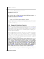
1.3
Desmond Calculations Overview
Desmond jobs should be started from well-prepared structures. For proteins it is recommended
that the protein be prepared with the Protein Preparation Wizard (see the Protein Preparation
Guide for details). For other types of molecules, such as ligands, the molecule should have a
fairly good Lewis structure (although there are some built-in capabilities for adjusting incorrect or non-optimal Lewis structures).
If you have MacroModel you can perform a quick check on the structure by performing a
Current Energy calculation (available from the MacroModel submenu of the Applications
menu) using the OPLS_2005 force field with the Solvent set to None. If that calculation
succeeds it is almost certain that Desmond and its associated tools will be able to work with
this structure as well. If the structure is problematic Maestro and MacroModel often provide
useful diagnostics for what might be wrong.
Performing a study based on a Desmond molecular dynamics simulation usually involves a
number of stages, including simulation setup, relaxing the system (this could just be a minimization), running the simulation, viewing trajectories, and analyzing the results. Simulation
setup is described in Chapter 2, the basic Desmond minimization, molecular dynamics, simulated annealing, and replica exchange tasks are described in Chapter 3. Simplified FEP setup
for relative binding and solvation free energies and absolute solvation free energies is
described in Chapter 4, along with restarting and customizing FEP simulations. Examining the
results, including viewing a trajectory, and analysis of results, is described in Chapter 5.
FEP jobs are handled differently due to the complexity of the calculations and the fact that the
overall goal for an FEP job is to produce one number: the free energy change. FEP jobs are
4
Desmond 2.2 User Manual
Chapter 1: Introduction
supported for specific types of calculations, using automated procedures that differ from those
used for individual, general purpose Desmond simulations.
The basic outline of a Desmond simulation as run from Maestro is as follows:
1. Import the structure file for the system of interest into Maestro.
2. Prepare the structure for simulation with the Protein Preparation Wizard. This step
involves removing ions and molecules (which are artifacts of crystallization), setting correct bond orders, adding hydrogens, filling in missing side chains or whole residues as
necessary, reorienting various groups and varying residue protonation states to optimize
the hydrogen bonding network, and then checking the structure carefully.
3. If your system is a membrane protein, embed the protein in the membrane. This step and
the next two steps are performed in the System Builder panel.
4. Generate a solvated system for simulation.
5. Distribute positive or negative counter ions to neutralize the system, and introduce additional ions to set the desired ionic strength (when necessary).
6. Relax the system either by minimization or by selecting the panel option to relax the
model system before simulation.
7. Set the simulation parameters in one of the general Desmond panels, for molecular
dynamics, simulated annealing, or replica exchange.
8. Run the simulation.
9. Analyze your results using the Trajectory Viewer and other analysis tools.
1.4
Citing Desmond in Publications
The use of this product should be acknowledged in publications as:
Desmond Molecular Dynamics System, version 2.2, D. E. Shaw Research, New York, NY,
2009. Maestro-Desmond Interoperability Tools, version 2.2, Schrödinger, New York, NY,
2009.
Please also include a reference to the following paper:
Kevin J. Bowers, Edmond Chow, Huafeng Xu, Ron O. Dror, Michael P. Eastwood, Brent A.
Gregersen, John L. Klepeis, Istvan Kolossvary, Mark A. Moraes, Federico D. Sacerdoti, John
K. Salmon, Yibing Shan, and David E. Shaw, “Scalable Algorithms for Molecular Dynamics
Simulations on Commodity Clusters,” Proceedings of the ACM/IEEE Conference on Supercomputing (SC06), Tampa, Florida, November 11-17, 2006.
Desmond 2.2 User Manual
5
6
Desmond 2.2 User Manual
Desmond User Manual
Chapter 2
Chapter 2:
Building a Model System
Performing simulations on aqueous biological systems requires the preparation of biological
molecules such as proteins and ligands, addition of counter ions to neutralize the system, selection of simulation box size, solvation of the solutes using explicit solvent molecules, and alignment of proteins to a membrane bilayer (if used). This procedure is often tedious if it has to be
performed manually. Tools for all these tasks are provided with Maestro.
Protein and ligand structures used in a Desmond simulation must be complete all-atom 3D
structures with a reasonable geometry. The preparation of protein and ligand structures for use
in a simulation can be done with the Protein Preparation Wizard and LigPrep. The Protein
Preparation Wizard corrects structural defects, adds hydrogen atoms, assigns bond orders, and
can selectively assign tautomerization and ionization states, and optimize the hydrogen
bonding network. For more information, see the Protein Preparation Guide. LigPrep performs
2D-to-3D conversion if necessary, adds hydrogen atoms, generates tautomers, ionization
states, ring conformations, and stereoisomers, as requested, and produces minimized 3D structures. For more information, see the LigPrep User Manual.
Once you have prepared the protein and ligand structures, you can proceed to the remaining
tasks in building a model system that can include proteins, ligands, explicit solvent, a
membrane, and counter ions. The System Builder automates this process and significantly
reduces the effort required. You can set up and run a System Builder job from the System
Builder panel, or from the command line. See Chapter 9 for information on running the System
Builder from the command line.
To open the System Builder panel, choose Applications > Desmond > System Builder in the
main window. Before you start working in this panel, display the solutes in the Workspace.
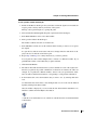
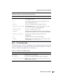
2.1
Adding Solvent
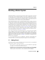
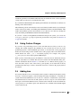
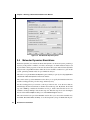
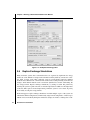
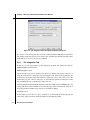
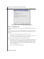
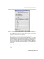
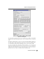
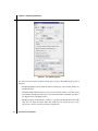
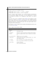
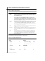
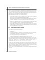
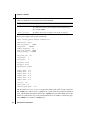
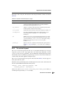
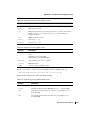
The solvation model is selected in the Solvation tab. You can choose from a set of predefined
solvent models, or specify a custom solvent model:
• None—Do not use a solvent. This option allows you to run a simulation on a pure liquid,
for example, or in vacuum (with a sufficiently large box).
• Predefined—Use one of the predefined solvent models, which you can select from the
option menu. The models include four water models, SPC, TIP3P, TIP4P, and TIP4PEW,
and three organic solvents, methanol, octanol, and dimethyl sulfoxide (DMSO).
Desmond 2.2 User Manual
7
Chapter 2: Building a Model System
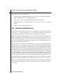
Figure 2.1. The Solvation tab of the System Builder panel.
• Custom—Import a custom solvent system from file. Enter the solvent system file name in
the text box, or click Browse and navigate to the solvent system file in the file selector
that is displayed.
The solvent is placed by replicating “boxes” of solvent molecules and deleting molecules
whose center of mass lies outside the periodic box boundary, and molecules that are inside or
have significant overlap with the solute or the membrane (if one is used).
2.2
Setting Up the Boundary Box
The periodic boundary conditions are set up by specifying the shape and size of the repeating
unit, or box, which you can do in the Solvation tab.
To set up the box, first choose the shape from the Box shape option menu. Three basic shapes
are provided: Cubic, Orthorhombic, and Triclinic. As special cases of the triclinic box shape,
three other shapes are supported: Truncated octahedron, Rhombic dodecahedron xy-square,
and Rhombic dodecahedron xy-hexagon.
8
Desmond 2.2 User Manual
Chapter 2: Building a Model System
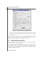
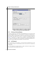
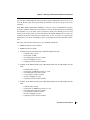
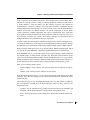
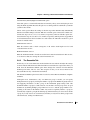
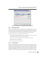
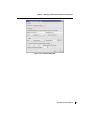
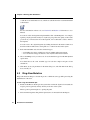
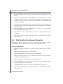
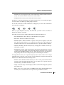
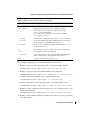
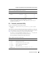
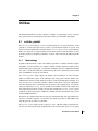
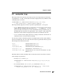
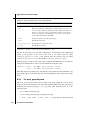
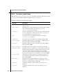
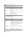
Figure 2.2. The Membrane Setup panel.
When you have chosen the box shape, you can choose whether to specify the size of the box in
terms of a buffer distance or as an absolute size, by selecting one of the Box size calculation
method options:
• Buffer—The simulation box size is calculated by using the given buffer distance between
the solute structures and the simulation box boundary.
• Absolute size—Specify the lengths of the sides of the simulation box size (and angles if
necessary).
Having chosen a method, you can specify the distances and angles in the Distances and Angles
text boxes. The text boxes that are available depend on the box shape. For all choices except a
truncated octahedron, the box can be displayed in the Workspace by selecting Show boundary
box.
If you want to calculate the volume of the box that encompasses the solutes, click Calculate.
The volume is displayed in the Box volume text box. To minimize the volume of the box, click
Minimize Volume. The solutes are reoriented so that the box volume is minimized.
2.3
Adding a Membrane
A membrane can be added to the system using the Set Up Membrane dialog box, which you
open by clicking Set Up Membrane in the Solvation tab. This dialog box allows you to select
and position the membrane; the actual membrane is added when the system builder job is run.
There are three predefined membranes, DPPC, POPC, and POPE, which you can choose by
selecting Predefined, and choosing the membrane from the option menu. The temperature at
Desmond 2.2 User Manual
9
Chapter 2: Building a Model System
which the membrane patch was preequilibrated is given in parentheses after the membrane
name. Because DPPC has a gel transition temperature around 313 K, the recommended
minimum simulation temperature is also 325 K.
If you want to position a custom membrane, select Custom, and enter the name of the Maestro
file containing the membrane model in the text box, or click Browse and navigate to the file.
If you have an existing membrane in a project entry that you want to use for the current model
system, you can load it by selecting the entry and clicking Load Membrane Position from
Selected Entry. The membrane from this entry is then used for the model system you are
building.
When you click Place Automatically, the membrane position is determined according to the
information available, as follows:
• If you have a protein from the OPM database (http://opm.phar.umich.edu), the membrane
is placed using the information provided with the protein.1
• Otherwise the surface of the membrane is placed perpendicular to the longest axis of the
protein.
• If transmembrane atoms are defined, they are placed inside the membrane. Placement of
transmembrane atoms inside the membrane takes precedence over placement perpendicular to the longest axis.
To define the transmembrane atoms, click Select, and use the Atom Selection dialog box
to select the desired atoms. For more information on this dialog box, see Section 5.3 of
the Maestro User Manual.
If you have a protein that is prealigned, you can click Place on Prealigned Structure to place
the membrane. The membrane is positioned symmetrically about the coordinate origin so that
its surfaces are parallel to the xy plane (perpendicular to the z axis). This means that the protein
must be aligned accordingly.
When you have placed the membrane, a representation of the membrane is displayed in the
Workspace. The representation consists of two red slabs for the surfaces, with a yellow line
perpendicular to the slab planes. After the membrane has been placed, you can adjust its orientation by selecting Adjust membrane position, and rotating the membrane. The actual
membrane molecules are placed when the system builder job is run. The molecules are placed
by replication of a membrane segment and deletion of molecules whose center of mass lies
1.
10
The PDB files in this database have an invalid positioning of the remark fields for the membrane information,
and must be fixed before use. To fix them, you can use the command
perl -pi -e 's#REMARK 1/2#REMARK
1/2#' *.pdb.
Here there are two spaces after the first REMARK and five after the second.
Desmond 2.2 User Manual
Chapter 2: Building a Model System
outside the periodic box boundaries. Molecules that are inside the solute or have significant
overlap with it are removed to accommodate the solute.
If you click Place Automatically after adjusting the membrane, the membrane is returned to its
default position and orientation.
The membrane position and orientation can be stored in Project Table entries, by selecting the
entries in the Project Table, and clicking Save Membrane Position to Selected Entries. This
enables the membrane position and orientation to be loaded at a later time by selecting the
entry and clicking Load Membrane Position from Selected Entry.
If you have a related, well-equilibrated membrane-bound protein system, you can use the
mold_gpcr_membrane.py script to replace the protein with a new protein. See Section 9.4
on page 90 for details.
2.4
Using Custom Charges
If you want to use partial charges from a source other than the force field, you can do so by
selecting Use custom charges in the Solvation tab. You can then choose from one of the
predefined properties on the Predefined option menu, or enter the name of the property that
defines the custom charges in the Custom text box. The property name is the internal name,
which should start with r_ (i.e. a real-valued property). For example, the property
r_j_ESP_Charges selects Jaguar-generated ESP charges.
When you have selected the property, click Select to select the atoms for which these charges
are to be used. There is no default. The selection is made in the Atom Selection dialog box,
which is described in detail in Section 5.3 of the Maestro User Manual. If the property you
chose has values only for some of the atoms (e.g. the ligand), you can select these atoms by
specifying the entire range of values. Atoms that do not have a value for the property will not
be selected.
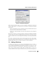
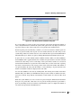
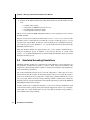
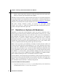
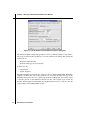
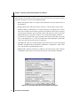
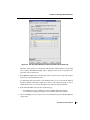
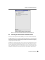
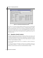
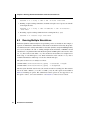
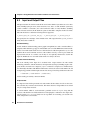
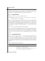
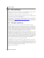
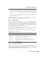
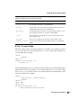
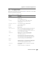
2.5
Adding Ions
It is usually desirable to have an electrically neutral system for simulation (though not strictly
necessary, as Desmond applies a uniform background charge distribution to neutralize the
system in the Ewald summation). You can choose to add ions to neutralize the system in the
Ion placement section of the Ions tab. The system can also be set up in a salt solution rather
than a pure solvent in the Add salt section of the Ions tab. To limit the locations in which ions
can be placed, you can define regions from which ions are excluded, in the Exclude region
section of the Ions tab.
Desmond 2.2 User Manual
11
Chapter 2: Building a Model System
Figure 2.3. The Ions tab of the System Builder panel.
2.5.1
Defining an Excluded Region
To define an excluded region, click Select in the Excluded region section of the Ions tab, and
use the Atom Selection dialog box to select the desired set of residues. You should select residues that are within or near the binding site. When ions are placed, they will not be placed near
these residues. The residues that you select are colored blue and rendered in CPK. See
Section 5.3 of the Maestro User Manual for more information on the Atom Selection dialog
box. The region is defined by the distance in the Exclude ion and salt placement within text box.
Ions will not be placed within the specified distance of the selected atoms.
2.5.2
Ion Placement
Ions are placed in the solvent according to your selection in the Ion placement section of the
Ions tab. Each ion replaces a solvent molecule. You can, of course, choose not to add ions, by
selecting None.
If you select Neutralize, the minimum number of sodium or chloride ions required to balance
the system charge is placed randomly in the solvent.
12
Desmond 2.2 User Manual
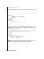
Chapter 2: Building a Model System
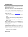
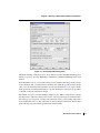
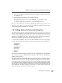
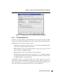
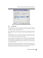
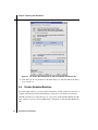
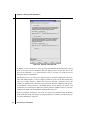
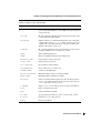
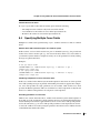
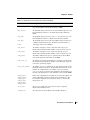
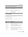
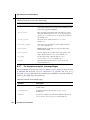
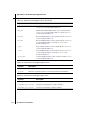
Figure 2.4. The Advanced Ion Placement dialog box.
If you select Add, you can choose the ion type from the option menu and enter the number of
ions to add (which need not neutralize the system). The option menu only displays ions that are
opposite in charge to that of the system. Ions are not placed in the excluded regions.
Instead of placing ions automatically, at random, you can locate and select suitable regions for
ions to be placed. Usually these regions are near residues that have the same charge as the
system charge and are not near the active site. You can define these regions in the Advanced Ion
Placement dialog box, which you open by clicking Advanced Ion Placement in the Ions tab.
To place the ions, you must identify suitable candidate residues. When you click Candidates,
the Candidates table is populated with a list of residues in regions that have not been excluded
and have the same charge as the overall charge of the system. These residues are colored red
and rendered in CPK. Ions are placed near the residues that you select in the table, replacing
the closest solvent molecule to the average position of the atoms in the residue. The number of
ions placed (initially 0), along with the number of ions remaining to be placed and the total
number of candidate residues are displayed above the table.
You can add candidates to the table by clicking New, and selecting the residues in the Atom
Selection dialog box. When you click OK in the dialog box, the residues are added to the table,
and can be selected along with the automatically located residues. To clear the table, click
Reset.
When the system builder job is run, ions that are placed using the Advanced Ion Placement
dialog box are placed first. Once these ions are placed, random placement is performed to
place any remaining ions that are needed to neutralized the system or complete the number of
ions selected for placement in the Add text box.
Desmond 2.2 User Manual
13
Chapter 2: Building a Model System
2.5.3
Adding a Salt
Adding a salt is relatively simple. To do so, first select the Add salt option. The controls in the
Add salt section are then activated, and you can enter the salt concentration, in mol dm–3, and
select the desired ions. If you select multiply charged ions, the concentration is taken from the
empirical formula for the salt. For example, for MgCl2 the concentration of Mg2+ would be the
specified concentration and the concentration of Cl– would be twice the specified concentration. A value of 0.15M is approximately the physiological concentration of monovalent ions.
When the salt ions are placed, they are randomly distributed in the solvent, and replace solvent
molecules. Salt ions are not placed in the excluded region defined in the Exclude region
section.
2.6
Running the Job
When you have finished making settings, you can set up and start the job immediately, or write
out the input file and run the job from the command line.
To set up and run the job, click Start. The Start dialog box opens, allowing you to name the
job, choose the host and set the user name (if necessary). System Builder jobs do not usually
take more than a few minutes, so you can run the job locally. You can also choose whether to
incorporate the output CMS file back into the Maestro project, by choosing Append new
entries from the Incorporate option menu. This is useful if you want to continue on to set up a
simulation in Maestro. If you choose Do not incorporate, the CMS file is placed in the current
working directory, but is not added to the project.
If you want to run the job from the command line, click Write. The Write dialog box opens, in
which you can specify a name and then write the file. The name is used to construct the file
names, by adding the appropriate extension.
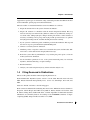
2.7
Quick Setup Instructions
The sets of instructions below take you through the simplest setup procedures. It is assumed
that you have imported the prepared protein and ligand structures into Maestro, and displayed
them in the Workspace.
To add solvent:
1. Select Predefined for the Solvent model option, and choose a model from the option
menu.
2. Choose a box shape.
14
Desmond 2.2 User Manual
Chapter 2: Building a Model System
3. Choose a box size calculation method—Buffer for adding a buffer region to the solutes, or
Absolute size for specifying the actual box size.
4. Enter buffer distances or side lengths in the available text boxes.
5. Enter angles if you selected Triclinic for the box shape.
To add ions:
1. In the Ions tab, choose an option for the addition of ions.
2. If you selected Add, enter the number of ions to add in the text box.
3. Choose an ion type from the option menu.
4. If the solvent is intended to be a salt solution, select Add salt.
5. Enter the desired salt concentration in the Salt concentration text box.
6. Choose positive and negative ion types from the Salt positive ion and Salt negative ion
option menus.
To add a membrane:
1. Click Add Membrane in the Solvation tab.
2. In the Membrane tab, select Predefined for the membrane model, and choose a membrane
type from the option menu.
3. Click Place Automatically.
4. Select Adjust membrane position and adjust the orientation of the membrane in the Workspace.
5. Click OK.
Click Start to run the job or click Write to write the input file.
Desmond 2.2 User Manual
15
16
Desmond 2.2 User Manual
Desmond User Manual
Chapter 3
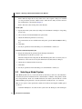
Chapter 3:
Running a Desmond Simulation from
Maestro
The general Desmond panels enable you to set up and run the main tasks available with
Desmond: molecular dynamics, minimization, simulated annealing, and replica exchange,
jobs. The panels are designed to make setting up these types of jobs as easy as possible, and
provide the most common simulation controls. The default values provided in the panels represent a good balance between accuracy and performance, and are adequate for most jobs
without change. For more control over the simulation parameters, you can make settings in the
Advanced Options dialog box, which is described in Section 3.8 on page 27.
A much more automated approach is provided for FEP simulations of binding and solvation
free energies in four specialized panels, Ligand Functional Group Mutation by FEP, Ring Atom
Mutation by FEP, Protein Residue Mutation by FEP, and Total Free Energy by FEP, for which a
model system and the additional parameters are set up automatically. These panels, and the
FEP panel for restarting and customizing these jobs, are described in Chapter 4.
In addition to setting up simulations, you can use the general panels to restart a simulation
from a checkpoint file as generated by a previously interrupted simulation.
All jobs run from these panels require a model system to be built first, in the System Builder
panel—see Chapter 2 for details.
Desmond simulations can also be run from the command line—see Chapter 6.
3.1
Overview of the General Desmond Panels
The general Desmond panels have two main sections: Model system, in which the model
system is chosen, and Simulation, in which the parameters for the task are set up. The controls
in the Simulation section depend on the panel. Specifying a model system is described in
Section 3.2 on page 18, and the various tasks are described in the subsequent sections.
At the bottom of the panel are the action buttons for the job:
• Start—Start the job. Opens the Start dialog box to set job parameters and submit the job
for execution. See Section 3.9 on page 36 for details. A general description of this dialog
box and its features is given in Section 2.2 of the Job Control Guide.
• Read—Read a configuration (.cfg) file, to set up the simulation. Opens a file selector in
which you can navigate to the desired file.
Desmond 2.2 User Manual
17
Chapter 3: Running a Desmond Simulation from Maestro
• Write—Write the input files for the job but do not start it. Opens a dialog box in which
you can provide the job name, which is used to name the files. The job can be run from
the command line, as described in Chapter 6.
• Reset—Reset the values in the panel to their defaults.
To run a job:
1. Specify the model system, either by loading it from the Maestro Workspace or importing
it from a file.
2. Choose the task from the Simulation task option menu.
3. Adjust the simulation parameters as necessary.
For parameters that are not available in the main panel, open the Advanced Options dialog
box.
4. Click Start.
5. Set the job parameters in the Start dialog box, and click Start to run the job.
To restart a molecular dynamics job:
1. Import the checkpoint file generated by the interrupted simulation.
The default name of this file is jobname.cpt.
When the checkpoint file is imported, the Run Desmond panel enters a read-only state, in
which most of the controls are set by the information read and cannot be changed.
2. Adjust the total simulation time if necessary.
3. Click Start.
4. Set the job parameters in the Start dialog box, and click Start to run the job.
3.2
Selecting a Model System
In the Model system section, you select the model system that you will use for the simulation.
A valid model system for simulations must contain both the coordinates of the particles and the
force field parameters. In the case of FEP simulations, the model system should also contain
additional FEP-specific parameters. A model system file normally has the .cms extension.
There are two options on the option menu, and the tools in this section depend on which option
you choose.
• Load from Workspace—Load the model system from the Workspace. The Workspace
18
Desmond 2.2 User Manual
Chapter 3: Running a Desmond Simulation from Maestro
must contain a model system that has already been prepared with the System Builder
panel. When you choose this item, the Load button is displayed, which you click to load
the model system from the Workspace.
• Import from file—Import the model system from a file. You can choose to import a model
system file (.cms) or a checkpoint file (.cpt).
If you import a model system file, it must contain a model system that has already been
prepared with the System Builder panel. When the file is imported, a message about the
system is displayed below the option menu.
If you import a checkpoint file, most of the panel controls are unavailable. The purpose of
the checkpoint file is to restart an interrupted simulation, so the parameters of the simulation cannot be altered. You can change the total simulation time, and then start the job.
3.3
Minimizations
Minimization jobs relax the system into a local energy minimum. The minimization task
performs minimization of the model system using a hybrid method of the steepest decent and
the limited-memory Broyden-Fletcher-Goldfarb-Shanno (LBFGS) algorithms. This task is set
up in the Minimization panel, which you open by choosing Applications > Desmond > Minimization in the main window.
There are only two parameters that can be set for this task:
• Maximum iterations—Enter the maximum number of iterations in this text box, or use the
arrow buttons to change the maximum number of iterations in steps of 10.
• Convergence Threshold—Enter the convergence threshold for the gradient in units of
kcal mol–1 Å–1.
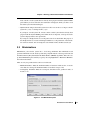
Figure 3.1. The Minimization panel.
Desmond 2.2 User Manual
19
Chapter 3: Running a Desmond Simulation from Maestro
Figure 3.2. The Molecular Dynamics panel.
3.4
Molecular Dynamics Simulations
Molecular dynamics jobs simulate the Newtonian dynamics of the model system, producing a
trajectory of the particle coordinates, velocities, and energies, on which statistical analyses can
be performed to derive properties of interest about the model system. The molecular dynamics
task performs a single MD simulation under the chosen ensemble condition for a given model
system, generating simulation data for post-simulation analyses.
This task is set up in the Molecular Dynamics panel, which you open by choosing Applications
> Desmond > Molecular Dynamics in the main window.
The controls at the top of the Simulation section allow you to specify the simulation time in ns
and the recording period in ps for the energy and the trajectory.
For the recording period you can enter a value in ps in the text box, or use the arrow buttons,
which change the time in increments of 50 times the far time step size. By default, the far time
step size is 0.006 ps, and thus the increments are 0.3 ps. Values entered in this text box are
rounded to an integer multiple of the far time step size. This time step size is set in the Integration tab of the Advanced Options dialog box, in the RESPA integrator section.
The controls in the lower part of the Simulation section allow you to choose the ensemble class,
from NVE, NVT, NPT, NPAT, and NPγT, to set the temperature (except for NVE) and the pres20
Desmond 2.2 User Manual
Chapter 3: Running a Desmond Simulation from Maestro
sure (except for NVE and NVT), and set the surface tension (NPγT only). It also allows you to
relax the model system before performing the simulation, and choose the protocol for the
relaxation.
When Relax model system before simulation is selected, a series of minimizations and short
molecular dynamics simulations are performed to relax the model system before performing
the simulation you set up. This option is selected by default, and a default protocol is used.
Usually, if the model system was just created from the System Builder panel, it needs to be
relaxed; if the model system has been relaxed before, it does not need to be relaxed again.
Alternatively, you can run a minimization prior to performing the molecular dynamics calculation.
The stages in the default relaxation process for the NPT ensemble are:
1. Minimize with the solute restrained
2. Minimize without restraints
3. Simulate in the NVT ensemble using a Berendsen thermostat with:
•
•
•
•
•
a simulation time of 12ps
a temperature of 10K
a fast temperature relaxation constant
velocity resampling every 1ps
non-hydrogen solute atoms restrained
4. Simulate in the NPT ensemble using a Berendsen thermostat and a Berendsen barostat
with:
•
•
•
•
•
•
a simulation time of 12ps
a temperature of 10K and a pressure of 1 atm
a fast temperature relaxation constant
a slow pressure relaxation constant
velocity resampling every 1ps
non-hydrogen solute atoms restrained
5. Simulate in the NPT ensemble using a Berendsen thermostat and a Berendsen barostat
with:
•
•
•
•
•
•
a simulation time of 24ps
a temperature of 300K and a pressure of 1 atm
a fast temperature relaxation constant
a slow pressure relaxation constant
velocity resampling every 1ps
non-hydrogen solute atoms restrained
Desmond 2.2 User Manual
21
Chapter 3: Running a Desmond Simulation from Maestro
6. Simulate in the NPT ensemble using a Berendsen thermostat and a Berendsen barostat
with:
•
•
•
•
a simulation time of 24ps
a temperature of 300K and a pressure of 1 atm
a fast temperature relaxation constant
a normal pressure relaxation constant
This protocol is used for the NPAT and NPγT ensembles as well. A similar protocol is used for
the NVT ensemble.
The protocol files can be found in $SCHRODINGER/mmshare-vversion/data/desmond. The
procedure follows a similar pattern as for NPT. If you want to modify the protocol, you can
copy these files and edit them. To make use of the modified protocol, click Browse and navigate to the new protocol file, which has a .msj extension. The file name is then listed in the
Relaxation protocol text box.
When the simulation finishes, the output structure file (.cms) is written to disk and incorporated into the Maestro project. In addition, a new trajectory directory is created, called
jobname_trj by default. Checkpoint files are written during the simulation, but are not written
during the relaxation process.
3.5
Simulated Annealing Simulations
Simulated annealing methods use a temperature program rather than a single temperature for
the simulation. A temperature program is a series of times and target temperatures. The
temperature is linearly interpolated as a function of time between adjacent target temperatures
and is controlled by a thermostat.
One of the predominant strategies used is to raise the temperature to a high value one or more
times before relaxing the system to the desired temperature. The goal is to permit the system to
relax out of an initial state that corresponds to a high energy potential minimum into a lower
state by crossing barriers in the free-energy landscape, which is achieved more effectively
during the periods of elavated temperatures. The default temperature program in the Simulated
Annealing panel falls into this catagory.
Another common use for simulated annealing is to perform an effective minimization with
some relaxation of the system by slowly decreasing the temperature down to very low temperatures. This slow cooling should permit at least some shifts from higher energy minima to
lower minima in the energy landscape.
22
Desmond 2.2 User Manual
Chapter 3: Running a Desmond Simulation from Maestro
Figure 3.3. The Simulated Annealing panel.
Simulated annealing calculations can be set up and run from the Simulated Annealing panel,
which you open by choosing Applications > Desmond > Simulated Annealing in the main
window.
In the Simulation section, you can make settings for the simulated annealing job. The settings
for the simulation time, recording interval, ensemble class and model system relaxation are the
same as for a molecular dynamics simulation, and are described in Section 3.4 on page 20. The
main specific task for simulated annealing is to provide information on the stages by providing
a schedule of reference temperature changes.
The number of stages is set in the Number of stages text box. When a value has been entered,
the table below is adjusted to display text boxes for each stage. The stages are indexed from 0.
For each stage you can specify a starting time in the Time text box, and a starting temperature
in the Temperature text box. The temperature is linearly interpolated between adjacent time
points. The last stage runs until the specified total simulation time.
Desmond 2.2 User Manual
23
Chapter 3: Running a Desmond Simulation from Maestro
Figure 3.4. The Replica Exchange panel.
3.6
Replica Exchange Simulations
Many molecular systems have conformations that are separated by significant free energy
barriers. It can be difficult to sample such conformations if they differ by concerted or collective shifts of many atoms. This commonly occurs in protein-ligand complexes. Random
methods such as Monte Carlo conformational searches have trouble generating such collective
changes, while thermal methods such as molecular dynamics have trouble surmounting the
free energy barriers. Replica exchange simulations [39] attempt to tackle this problem by
allowing the system to spend some time at elevated temperatures in addition to the temperature
of interest. Time spent at elevated temperatures permits the system to evolve faster, in part by
more readily crossing free energy barriers.
Desmond supports replica exchange simulations in which multiple copies of the system are
simulated at different temperatures, which usually range from the temperature of interest up to
700 K or more. Periodically during the simulation, attempts are made to exchange the coordi24
Desmond 2.2 User Manual
Chapter 3: Running a Desmond Simulation from Maestro
nates of copies that are at different temperatues. The exchange is processed in a Monte Carlolike process: select the systems to attempt to exchange and then use a Metropolis-like criterion
to decide whether to accept the change [39]. The exchange acceptance ratio satisfies the
detailed balance or balance condition so that each replica remains in equilibrium after the
exchange. When many such exchanges are accepted over the course of an extended simulation,
multiple systems with very different histories can visit the temperature of interest. While
systems spend time at higher temperatures they explore conformational space signficantly
more rapidly than if they remained at the target temperature. Thus the composite trajectory at
the temperature of interest may contain a more diverse collection of conformations than if
multiple simulations were performed at the target temperature.
As with a regular molecular dynamics simulation each replica may be run on multiple processors. Since the simulations of each replica proceeds independently between exchange attempts
the additional level of parallelization achieved by running multiple replicas is highly efficient.
Replica exchange simulations can be set up and run from the Replica Exchange panel, which
you open by choosing Applications > Desmond > Replica Exchange in the main window.
In the Simulation section, you can make settings for the replica exchange job. The settings for
the simulation time, recording interval, ensemble class and model system relaxation are the
same as for a molecular dynamics simulation, and are described in Section 3.4 on page 20. The
default ensemble for replica exchange is NVT. The main specific task for replica exchange is to
provide information on the exchange scheme, temperature range and temperature profile.
There are two exchange scheme options:
• nearest neighbor—allow exchange only between replicas that are adjacent in temperature.
• random—allow exchange between randomly chosen replicas.
In the Exchange attempt text boxes, you can set the starting time and the interval for making
exchanges, in ps. The first exchange occurs at the specified starting time and thereafter at the
specified interval.
The temperature range is set in the Temperature range text boxes. The defaults are 300 K for
the low temperature and 800 K for the high temperature. There are three options for the
temperature profile:
• quadratic—Set the temperatures by quadratic interpolation between the minimum and
maximum, with the high temperature at the maximum of the quadratic curve.
• linear—Set the temperatures by linear interpolation between the maximum and the minimum.
Desmond 2.2 User Manual
25
Chapter 3: Running a Desmond Simulation from Maestro
• manual—Set the temperatures manually, by editing the temperatures in the replica table.
When you select this option the table becomes editable.
Information on the temperatures is displayed in the replica table. You can edit the temperatures
by selecting manual for the temperature profile. Some guidance on selecting temperatures is
available in Ref. 40. Setting up the temperatures and the number of replicas for a meaningful
simulation can be difficult. For assistance with this task, contact [email protected].
The replica exchange simulation produces one trajectory for each replica, labeled
jobname_replicanum_trj, where num is the index of the replica, starting from 0, and corresponds to the replica index in the replica table.
3.7
Simulations on Systems with Membranes
Simulations of systems that contain membranes require some special consideration. This is
because nearly all current all-atom membrane potential models in existence do not, on their
own, maintain the appropriate surface areas on the time scale of tens of ns in simulations of
pure membranes. If non-lipid components make up a significant fraction of the membrane
region (such as a protein in a relatively small amount of lipid), this issue is much less
pronounced and many not require special treatment. In this case the semi-isotropic NPT
ensemble may work well. However, if the simulated membrane is pure or only contains a small
solute (e.g. ligand-sized) the following practical approach may be useful.
When a solute is placed in a pure membrane, some lipids are usually removed to make room
for the new molecule during the system building process. As a result, adjustment of the surface
area of the solute + membrane system is often needed. This can usually be done using a fairly
short semi-isotropic simulation of up to about 0.5ns. When simulating beyond that time range
it is recommended to switch to either a constant surface area, constant normal pressure simulation (NPAT) or a constant surface tension simulation (NPγT). If the latter is selected we
suggest using a surface tension of 2000 bar/Å for DPPC and 4000 bar/Å for POPE and POPC.
We recommend examining the results of all membrane simulations carefully.
It can be difficult to relax freshly built protein-membrane systems. In particular, penetration of
the water between the protein than the lipids can be problematic and require very lengthy simulations to correct. A relaxation protocol, desmond_membrane_relax.msj, is available from
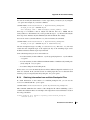
the command line that should reduce or eliminate such problems.
To use the membrane relaxation protocol:
1. Copy desmond_membrane_relax.msj to your working directory from the directory
$SCHRODINGER/mmshare-vversion/data/desmond/.
26
Desmond 2.2 User Manual
Chapter 3: Running a Desmond Simulation from Maestro
2. Save your newly built protein-membrane system in a CMS file ( referred to here as protein-membrane.cms.
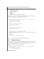
3. Run the membrane relaxation protocol using the command:
$SCHRODINGER/utilities/multisim -JOBNAME protein-membrane -HOST
localhost -host myhost -cpu cpus -i protein-membrane.cms
-m desmond_membrane_relax.msj -o protein-membrane-out.cms
This process may take hours to days since it equilbrates the system in stages for about 1.2 ns.
The file protein-membrane-out.cms should be reasonably well equilibrated and can be used
as input for the production simulation for your study.
3.8
Setting Options for Desmond Simulations
The default settings used in the Desmond panels were selected to produce good results in the
majority of cases. At times, you may want greater control over the parameters of the calculation. The Advanced Options dialog box provides access to advanced options for control of the
simulation or the minimization, such as the frequency of data output, integration time step
sizes, thermostat and barostat parameters, restraints, cutoff radii, and so on.
To open the Advanced Options dialog box, click Advanced Options in the Desmond panel that
you have open. This panel has several tabs, which are described in the following subsections.
•
•
•
•
•
•
•
Integration tab
Ensemble tab
Minimization tab
Interaction tab
Restraint tab
Output tab
Misc tab
The selection of tabs that is displayed depends on the task. For minimizations, only the Minimization, Interaction, Restraints, and Misc tabs are displayed. For MD simulations all but the Minimization tab are displayed.
The settings in this dialog box and the settings in the Desmond panels are not entirely independent, and can affect each other. For example, changing the far time step can affect the values of
the recording periods in the panel, because the latter are automatically rounded by the far time
step. As another example, changing the temperature or pressure in the Desmond panel updates
the temperature or pressure parameters in the dialog box. Changes in the Desmond panel take
effect immediately and update parameters in the dialog box, whereas changes made in the
dialog box only take effect when you click OK or Apply.
Desmond 2.2 User Manual
27
Chapter 3: Running a Desmond Simulation from Maestro
Figure 3.5. The Integration tab of the Advanced Options dialog box.
If you want to clear changes that have not been committed with the Apply button, click Reset.
Any changes made since the last set of changes were committed are discarded, and the values
in the dialog box are reset to the last set committed.
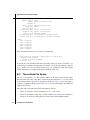
3.8.1
The Integration Tab
In this tab, you can set parameters for the integration algorithm. The tab has two sections,
RESPA integrator, and Constraint.
RESPA integrator section
Specify the time steps in fs for bonded, near, and far, by entering values in the text boxes, or
using the arrow buttons to change the value in increments of the bonded time step. Because the
bonded, near, and far time steps must maintain a certain ratio, when a new value is set for the
bonded time step, the other two time steps are automatically updated according the current
ratio. Changing the near or far time steps adjusts this ratio.
Selecting Set time step automatically based on constraint setting couples the RESPA time step
settings with those in the Constraint section. The time steps will be automatically set based on
the settings in the Constraint section, and are not available for editing.
Constraint section
In this section you can choose to apply constraints to covalent bonds between hydrogen and
other atoms, and set tolerances and iteration limits for the Shake algorithm.
28
Desmond 2.2 User Manual
Chapter 3: Running a Desmond Simulation from Maestro
Constrain heavy atom-hydrogen covalent bonds option
Select this option to constrain all bonds that are formed by a heavy atom and a hydrogen atom
using the Shake algorithm. Deselect this option to use bond potentials as defined in your model
system for these bonds.
Choice of this option affects the settings of the time steps when Set time steps automatically
based on constraint setting is selected. With the constraint option selected, the bonded, near,
and far time steps are set to 2 fs, 2 fs, and 6 fs, respectively; whereas with this option deselected, the time steps are set to 0.5 fs, 2 fs, and 6 fs, respectively. The larger time step permitted
for bonded interactions when constraints are used reduces the CPU time needed for a given
amount of simulation time.
Shake tolerance text box
Enter the tolerance used to check convergence of the relative bond length error for bond
constraints in the text box.
Maximum iterations text box
Enter the maximum number of iterations used in bond constraint calculations in this text box,
or use the arrow buttons to change the value in increments of 1.
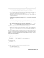
3.8.2
The Ensemble Tab
In this tab you can set the thermostat method and the barostat method and adjust the settings
for these methods. The thermostat method and the barostat method are coupled: the choice you
make from the Thermostat method option menu changes the selection from the Barostat
method option menu, and vice versa. The exception is that you can choose None for the
barostat method for any of the thermostat methods.
The Thermostat method option menu offers four choices: Nose-Hoover, Berendsen, Langevin,
and None.
Although in most circumstances, only one thermostat group is needed, you can specify
multiple thermostat groups by entering the number of groups in the Number of groups text box
and supplying information on these groups in the Thermostat group settings table. The
maximum number of groups is 8. The selection of atoms that is in each group can be set up in
the Misc tab, by defining multiple groups named thermostat, with the group numbers corresponding to the entries in the Values column. Any atoms not explicitly added to a group are
automatically assigned to group 0, the default group. This means that you do not need to define
a group if you only want to use one thermostat, and that you only need to define groups for the
extra thermostats, starting from thermostat 1.
Desmond 2.2 User Manual
29
Chapter 3: Running a Desmond Simulation from Maestro
Figure 3.6. The Ensemble tab of the Advanced Options dialog box.
The Thermostat group settings table provides text boxes for making settings for each thermostat group. For the Nosé-Hoover method, you can also make barostat settings. The settings that
can be made are:
• Reference temperature (K)
• Relaxation time (ps) (not for Langevin)
Nosé-Hoover only:
• Chain length
• Update frequency
The Barostat method option menu also offers four choices: Martyna-Tobias-Klein, Berendsen,
Langevin, and None. For each of these methods you can set the relaxation time (ps) in the
Relaxation time text box, choose a coupling style from the Coupling style option menu, and set
a reference pressure in the Reference pressure text box. The coupling style choices are
Isotropic, Semi-isotropic, and Anisotropic. For the Berendsen barostat, you can also enter the
compressibility in the Compressibility text box.
30
Desmond 2.2 User Manual
Chapter 3: Running a Desmond Simulation from Maestro
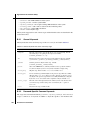
Figure 3.7. The Minimization tab of the Advanced Options dialog box.
3.8.3
The Minimization Tab
In this tab you can set parameters for the minimization, and also specify the output file. Minimization is performed with the LBFGS method, with an optional steepest descent initial phase.
The Minimizer section provides the following controls:
• LBFGS vectors—Specify the number of history vectors used by the LBFGS minimizer
for the update of the Hessian. The maximum is 6.
• Minimum SD steps—Specify the minimum number of steepest descent steps to be used
before switching to the LBFGS minimizer.
• Maximum step size—Specify the maximum step size in angstroms.
• Gradient threshold—Specify the gradient value in kcal mol–1 Å–1 at which the minimization method switches from steepest descent to LBFGS. The gradient is checked only after
the minimum number of steps is performed.
In the Output section you can specify the name of the structure output file. You can use
$JOBNAME as a variable representing the job name that you will set when you start the job or
write out the input files. You can also select Monitor structural change in minimization if you
want results returned to the Workspace during the course of the minimization.
Desmond 2.2 User Manual
31
Chapter 3: Running a Desmond Simulation from Maestro
Figure 3.8. The Interaction tab of the Advanced Options dialog box.
3.8.4
The Interaction Tab
In this tab you can specify how the short-range and long-range Coulombic interactions are
handled.
To define the short-range region, choose a method from the Short range method option menu.
The controls below this menu depend on the method chosen, which can be one of the
following:
• Cutoff—Enter a value in the Cutoff radius text box. The default is 9.0 Å.
• Force tapering or Potential tapering—Specify the range in angstroms over which the
force or the potential is tapered off in the two Tapering range text boxes.
There are two choices for handling the long-range Coulombic interactions:
• Smooth particle mesh Ewald—use the smooth particle mesh Ewald method. This method
requires a tolerance to be set in the Ewald tolerance text box. This tolerance affects the
accuracy of the long-range Coulombic interactions. The smaller the tolerance is, the more
accurate the computation of the long-range Coulombic interactions is, but the simulation
will be correspondingly slower.
• None—use the unmodified Coulomb interaction.
32
Desmond 2.2 User Manual
Chapter 3: Running a Desmond Simulation from Maestro
Figure 3.9. The Restraints tab of the Advanced Options dialog box.
3.8.5
The Restraints Tab
In this tab you can specify restraints on atom positions. A restraint is defined by a set of atoms
and a force constant. The restraints are listed in the restraints table. The Atoms column is filled
in automatically when you click Select and use the Atom Selection dialog box to specify the
atoms. You must enter the force constant in the table manually, by editing the table cell.
To manage the restraints, you can use the buttons beside the table:
• Select—Opens the Atom Selection dialog box to specify the atoms for the selected
restraint. Only available if a single row is selected in the table.
• Add—Adds a row to the restraints table so that a new restraint can be defined.
• Delete—Deletes the selected restraints.
• Reset—Resets the table to its default state.
3.8.6
The Output Tab
In this tab you can set names for various output files, and set the times for which recording in
these files begins, and the update frequency. For each file there is a starting time text box, in
which you can enter the starting time for recording of information to this file or adjust the
starting time in increments of 50 times the far time step (except for the checkpoint file, where
the increment is 5000 times the far time step). Some files also have an interval text box, in
which you can enter or adjust the recording interval (in the same increments as the starting
Desmond 2.2 User Manual
33
Chapter 3: Running a Desmond Simulation from Maestro
time). The files are listed below, with any extra controls. The intervals for the energy sequence
file and for the trajectory can be set in the Desmond panel.
• Status message file—This file contains general information about the current status of
the simulation.
• Energy sequence file—This file contains a sequence of various energies of the system.
• Trajectory directory—This directory is used by Desmond to periodically write out files
that record coordinates and velocities (optional) of all particles in the system at a particular point in the simulation. You can provide a title for the trajectory, and you can select
Record velocities if you want the velocities to be recorded along with the coordinates.
To ensure that associated solutes appear together in the trajectory rather than on opposite
sides of the simulation box, you can select Glue close solute molecules together. This
option only affects the way the trajectory is displayed.
• Checkpoint file—This file contains information that can be used to restart an interrupted
simulation. Checkpoint files permit bitwise continuation of simulations, so they can be
large, and should be saved infrequently if at all.
• Monitoring file—This file contains the coordinates of all particles in the system. This file
is in Maestro format and is used to monitor the progress of the simulation in Maestro.
Figure 3.10. The Output tab of the Advanced Options dialog box.
34
Desmond 2.2 User Manual
Chapter 3: Running a Desmond Simulation from Maestro
Figure 3.11. The Misc tab of the Advanced Options dialog box.
3.8.7
The Misc Tab
This tab provides access to various options that do not fit into the other categories. In this tab
you can initialize the velocities using a random number and a target temperature, and specify
atom groups for special treatment in the simulation.
Select Initialize velocities to initialize the velocities using the seed specified in the Random
number seed text box and the target temperature specified in the Target temperature text box,
in kelvin.
In the Atom group section you can specify atom groups. Atom groups are used for various
special treatments of atoms in the simulation. For example, if you define the frozen atom
group, the atoms in this group will be frozen in the simulation.
You can define multiple groups with the same name but a different index by setting the index in
the Value column. If you use multiple thermostats, for example, you can define the atoms in
each thermostat group by naming the group thermostat and setting the index to the thermostat group number in the Ensemble tab. Group 0 is the default group, to which all unassigned
atoms automatically belong.
The atom groups are listed in the table. The Atoms column is filled in automatically when you
click Select and use the Atom Selection dialog box to specify the atoms. Otherwise you can
edit this column to specify the ASL expression for the atoms in the group. The number of
atoms defined by the ASL expression is shown in the No. of Atoms column.
Desmond 2.2 User Manual
35
Chapter 3: Running a Desmond Simulation from Maestro
Beside the table are the following buttons:
• Select—Opens the Atom Selection dialog box to specify the atoms for the selected group.
Only available if a single row is selected in the table.
• Add—Adds an atom group. Clicking this button adds a row to the table.
• Delete—Deletes the selected groups. This operation can only be done on user-defined
groups.
• Reset—Resets the table to its default state.
3.9
Running a Simulation Job
Once you have finished making settings, you can click Start to set up the job parameters and
run the job, or you can click Write to write out the input files and run the job from the
command line. For information on running from the command line, see Chapter 6.
When you click Start, the Start dialog box opens. The common features of this dialog box,
such as the Output section, the Name, Username, and CPUs text boxes, and the Host option
menu, are described in Section 2.2 of the Job Control Guide. These features allow you to direct
the job to the appropriate host with the desired number of processors, and decide how to incorporate the output into the Maestro project.
For Desmond jobs, the choice of the number of processors has some special requirements.
Desmond uses a Cartesian domain decomposition of the simulation for efficient processing
This decomposition is described in the Desmond User’s Guide, provided by D. E. Shaw
Research. The details of the decomposition can be displayed in the Start dialog box by clicking
the Details button. You can control the decomposition by entering values in the x, y, and z text
boxes. The values you enter must be a power of 2. The decomposition is done automatically if
you enter a number in the CPUs text box. However, if you enter a number that is not a power of
2, the actual number of processors used is the largest power of 2 that is smaller than the
number you entered. The number of processors actually used is displayed in the details section.
To hide the details, click the Details button again. (It is possible to use a decomposition that is
not in powers of 2 when running from the command line—see the Desmond User’s Guide.)
Before you can run Desmond jobs in parallel, you must perform the necessary configuration of
the hosts file and any queues that you want to use. Details are given in Chapter 6 of the Installation Guide.
36
Desmond 2.2 User Manual
Chapter 3: Running a Desmond Simulation from Maestro
Figure 3.12. The Start dialog box.
Desmond 2.2 User Manual
37
38
Desmond 2.2 User Manual
Desmond User Manual
Chapter 4
Chapter 4:
Running FEP Simulations
Maestro provides panels for quickly setting up FEP simulations for certain common scenarios:
• Mutation of ligand functional groups: a group attached to a ligand by a single bond is
mutated to some other group.
• Aromatic ring atom substitution: an atom (with its attached hydrogens) is mutated into
another atom, usually a heteroatom.
• Protein residue mutation: the side chain of a protein residue is mutated into that of
another residue.
In these three scenarios, the binding free energy of the ligand can be calculated. For the first
two, the solvation free energy of the ligand relative to the original ligand can be calculated.
Total (absolute) solvation free energies can also be calculated for a ligand or a molecule, which
is done by annihilating the chosen molecule in the FEP simulation.
Free energy perturbation calculations are resource-intensive. While it is possible with the FEP
panels to set up multiple mutations in a single calculation, we recommend that only one mutation be performed per calculation due to the resource requirements.
4.1
FEP Panels
The FEP panels are designed to make setting up FEP jobs as easy as possible: most of the
computational details, such as setting the force field parameters, solvation, relaxation of the
system, and simulation time, are taken care of automatically. These predetermined parameters
for the FEP calculations should work for most systems, but you can also write out the input
files and then modify the simulation parameters in the FEP panel—see Section 4.8 on page 50.
(Note that checkpoint files are not written out for the relaxation stages.)
The panels for these calculation types have a common design. Each panel has a Define Perturbation tab, in which you set up the systems to be simulated, and a Plan Calculation tab, in
which you choose the environment (complex, pure solvent, vacuum) for the ligand and choose
the FEP protocol, which includes the ensemble. Information on setting up the system is
contained in the next few sections, followed by a section describing the Plan Calculation tab.
Desmond 2.2 User Manual
39
Chapter 4: Running FEP Simulations
The panels have action buttons at the bottom:
• Start—Opens the Start dialog box, in which you can set the job parameters such as job
name, host, number of CPUs, and so on, and then start the job. The general layout of this
dialog box is described in Section 2.2 of the Job Control Guide. The Desmond-specific
features of the Start dialog box and the issues in choosing the number of CPUs are
described in Section 3.9 on page 36.
• Write—Writes the input files for the job but does not start the job. Opens a dialog box in
which you can specify a job name, which is used to name the files. This capability is useful if you want to change the FEP protocol.
• Reset—Resets the entire panel to its initial state. This includes clearing the Workspace. If
you want to use the same structures, you will have to redisplay them before proceeding.
4.2
Ligand Functional Group Mutation
In ligand mutation, a group on the ligand molecule, called the substitution group, is replaced
with selected fragments. These fragments are chosen from a list of small, predefined fragments. The fragments can be adjusted to reduce steric clashes, and can be modified by using
the tools on the Build toolbar or in the Build panel.
The FEP calculations for ligand mutation are set up in the Ligand Functional Group Mutation by
FEP panel, which you open by choosing Desmond from the Applications menu, then choosing
Ligand Functional Group Mutation by FEP.
To run a ligand mutation job:
1. Include in the Maestro Workspace the system that contains the ligand to be mutated, the
receptor protein (optional), and any other key molecules of the system.
This step can be performed prior to opening the panel.
2. Select Pick the attachment bond, then pick the attachment bond in the Workspace, at the
end toward the substitution group.
This bond is the bond at which the substitution will take place. When the bond is picked,
a green arrow is drawn over the bond, pointing to the substitution group, and the ligand
core is colored with green carbons. If you clicked on the wrong end of the bond, click
again to correct the error. Once focus is returned to the panel, this option is deselected.
3. In the Fragment library table, select the fragments that you want to use to replace the original substitution group, by selecting their table rows.
Use shift-click and control-click to select multiple table rows. You can view the mutated
ligand by clicking in the View column.
40
Desmond 2.2 User Manual
Chapter 4: Running FEP Simulations
Figure 4.1. The Ligand Functional Group Mutation by FEP panel, Define Perturbation tab.
Since each FEP mutation requires a large amount of CPU time and space, we recommend
performing only one mutation in a given calculation.
4. (Optional) Display the mutated ligand and make adjustments to the fragment.
The adjusted fragment is used as the starting point in the FEP simulations. It is possible
that the fragment may have clashes with the protein in its default orientation or be in an in
appropriate conformation. The barriers between local minima in the potential energy surface can be large, and thus take a long time to cross during a simulation. Adjusting the
conformation can reduce clashes and help the simulation to sample the appropriate
conformations.
Once the fragment is displayed, you can reorient the fragment with the adjustment tools,
which are available from the Adjust toolbar button:
Desmond 2.2 User Manual
41
Chapter 4: Running FEP Simulations
or with the local transformation tools, which are available from the Local transformation
toolbar button:
For more information on these tools, see Section 4.8 and Section 7.2 of the Maestro User
Manual.
You can also add to the fragment using the Build toolbar or the Build panel—for example,
replacing a hydrogen with a methyl or a hydroxyl group. Since the quality of the results
goes down as you increase the size of the fragment, it is not advisable to add too much to
the fragment.
You can revert to the original fragment by clicking the button in the Reset column. You
should not make modifications to the ligand core or other molecules in the system.
5. In the Plan Calculation tab, select the calculation types:
• For binding free energy calculations, select In complex and In pure solvent.
• For solvation free energy calculations, select In pure solvent and In vacuum.
6. Choose the FEP protocol you want to use for each calculation type from the FEP protocol
option menu.
You should choose the same ensemble type for both the complex and pure solvent
calculations.
7. Click Start, set the job parameters in the Start dialog box, and click Start in the dialog
box to run the job.
4.3
Ring Atom Mutation
Ring atom mutation changes a selected ring atom to a different atom type while preserving the
hybridization of the atom.
To run a ring atom mutation job:
1. Include in the Maestro Workspace the system that contains the ligand to be mutated, the
receptor protein (optional), and any other key molecules of the system.
This step can be performed prior to opening the panel.
2. Select Pick the ring atom, then pick the ligand atom to be mutated in the Workspace.
42
Desmond 2.2 User Manual
Chapter 4: Running FEP Simulations
Figure 4.2. The Ring Atom Mutation by FEP panel, Define Perturbation tab.
When the atom is picked, it is rendered in ball-and-stick, and the ligand is colored with
green carbons. The Mutation targets table is displayed. Once focus is returned to the
panel, this option is deselected.
3. In the Mutation targets table, select the targets that you want to use to replace the original
ring atom by selecting their table rows.
Use shift-click and control-click to select multiple table rows. You can view the mutated
ligand by clicking in the View column. If you want to add a functional group as well as
mutate the ring atom, you can use the build tools to add to the mutated structure.
4. In the Plan Calculation tab, select the calculation types:
• For binding free energy calculations, select In complex and In pure solvent.
• For solvation free energy calculations, select In pure solvent and In vacuum.
5. Choose the FEP protocol you want to use for each calculation type from the FEP protocol
option menu.
Desmond 2.2 User Manual
43
Chapter 4: Running FEP Simulations
Figure 4.3. The Protein Residue Mutation by FEP panel, Define Perturbation tab.
6. Click Start, set the job parameters in the Start dialog box, and click Start in the dialog
box to run the job.
4.4
Protein Residue Mutation
In protein residue mutation, a protein residue is mutated into another residue in the presence of
a ligand, and the change in the ligand binding free energy due to the mutation is calculated.
The FEP calculations for ligand mutation are set up in the Protein Residue Mutation by FEP
panel, which you open by choosing Applications > Desmond > Protein Residue Mutation by
FEP.
44
Desmond 2.2 User Manual
Chapter 4: Running FEP Simulations
To run a protein residue mutation job:
1. Include in the Maestro Workspace the system that contains the ligand to be mutated, the
receptor protein, and any other key molecules of the system.
This step can be performed prior to opening the panel.
2. Select Pick atom to identify ligand, then pick a ligand atom in the Workspace.
3. In the Define Mutations section, select Pick residue.
4. Pick a protein residue in the Workspace.
The residue is added to the table as a mutation site.
5. In the Substitutes column, choose the residue from the list that you want to use to replace
the original.
To open the list, click the arrow button. The arrow changes direction and the list is displayed. To close it click the arrow button again.
6. Repeat Step 4 and Step 5 for as many mutations as you want to perform.
You can pick the same residue multiple times to mutate it to different residues. If you
pick different residues, each residue that you pick is mutated.
7. Click Generate Mutants.
8. The table is filled with the mutations that you have defined. For each of the original residues that you picked, all possible combinations of mutations are added to the table. For
example, if you picked two different residues, and for each you specified three substitutes, the table would list nine mutations, corresponding to each possible combination.
9. In the mutants table, select the mutations that you want to use, by selecting their table
rows.
Use shift-click and control-click to select multiple table rows. You can view the mutated
ligand by clicking in the View column.
Once the residue is displayed, you can reorient the side chain with the adjustment tools,
which are available from the Adjust toolbar button:
or with the local transformation tools, which are available from the Local transformation
toolbar button:
Desmond 2.2 User Manual
45
Chapter 4: Running FEP Simulations
For more information on these tools, see Section 4.8 and Section 7.2 of the Maestro User
Manual.
You can also modify the residue using the Build toolbar or the Build panel—for example
to replace sulfur with selenium, or to phosphorylate the residue. Since the quality of the
results goes down as you increase the size of the perturbation, it is not advisable to add
too much to the residue.
You can revert to the original residue orientation and structure by clicking the button in
the Reset column. You should not make modifications to the ligand core or other molecules in the system.
10. In the Plan Calculation tab, choose the FEP protocol you want to use for each calculation
type from the FEP protocol option menu.
You should choose the same ensemble type for both the complex and pure solvent
calculations.
11. Click Start, set the job parameters in the Start dialog box, and click Start in the dialog
box to run the job.
4.5
Total Solvation Free Energy Calculation
Calculating the absolute solvation free energy for a molecule involves running an “annihilation” FEP simulation, in which the selected molecule is removed from the system.
To run an annihilation job:
1. Include in the Maestro Workspace the system that contains the molecule to be annihilated.
This step can be performed prior to opening the panel.
2. Select Pick the molecule, then pick the molecule in the Workspace.
When the molecule is picked, it is colored with green carbons. Once focus is returned to
the panel, this option is deselected.
3. In the Plan Calculation tab, ensure that In pure solvent is selected.
4. Choose the FEP protocol you want to use for each calculation type from the FEP protocol
option menu and make any related settings.
The default simulation time is 2 ns, which is recommended for accurate results.
5. Click Start, set the job parameters in the Start dialog box, and click Start in the dialog
box to run the job.
46
Desmond 2.2 User Manual
Chapter 4: Running FEP Simulations
Figure 4.4. The Total Free Energy by FEP panel, Define Perturbation tab.
4.6
Selecting the Environment and FEP Protocol
The selection of the ligand environment and FEP protocol is made in the Plan Calculation tab.
The FEP simulations can be performed in three ligand environments: in the protein-ligand
complex (with solvent), in pure solvent, and in vacuum. This permits the calculation of binding
free energies, by selecting In complex and In pure solvent, and of solvation free energies, by
selecting In pure solvent and In vacuum.
The FEP protocol defines in detail how system is solvated, relaxed, and simulated. Four main
protocols are provided in the FEP protocol option menu for the complex and pure solvent: two
ensembles, Desmond NPT and Desmond NVT, with two options for the relaxation part (standard, or quick relaxation). The protocol for the simulation is the same for both ensembles (NVT
and NPT). For calculations in vacuum, there is the choice of the standard or quick relaxation.
Desmond 2.2 User Manual
47
Chapter 4: Running FEP Simulations
Figure 4.5. The Plan Calculation tab.
In addition you can read in a protocol by choosing User defined from the FEP protocol option
menu. A file name text box and Browse button is displayed. You can enter the name of the
protocol file (which has a .msj extension) in the text box, or navigate to it in the file selector
that opens when you click Browse.
The default protocol is as follows. The original system is solvated by adding SPC water molecules with a buffer distance of 5 Å for complexes and 10 Å for pure solvent. The vacuum simulation uses a buffer distance of 100 Å. The system goes through a relaxation process that
includes two minimizations followed by 4 short molecular dynamics simulations. The production simulation is run for 0.6 ns for each lambda window, and 12 windows are used for each
perturbation. You can change the buffer size and the production simulation time for each environment in the Buffer size and Production simulation time text boxes.
After the production simulations, the results are collected and analyzed using the Bennett
method. The final result (free energy) for each perturbation is recorded as an entry-level property in the final Maestro output file.
48
Desmond 2.2 User Manual
Chapter 4: Running FEP Simulations
4.7
FEP Results
The results of FEP calculations usually need some further processing to produce the quantities
of interest. The most common of these are discussed in the sections below.
4.7.1
Relative Free-Energy Differences
The estimated changes in free energy for FEP calculations are recorded as structure-level properties in the mutated structures (rather than in the original structures) in the output structure
file. For ligand functional group mutation, protein residue mutation and ring atom mutation,
these values are displayed in Maestro as dG jobname, and recorded in the file as
s_des_dG_jobname, where jobname is the name for the multisim job and usually ends in
_vacuum, _solvent or _complex for the corresponding environments (vacuum, pure
solvent, and complex). These values are strings rather than real numbers because they include
the estimated uncertainty. To obtain a relative solvation free energy, subtract the vacuum result
from the solvent result. Similarly relative binding free energies are calculated by subtracting
the solvent result from the complex result.
You can use the script calculate_ddg.py to take the difference between the values in two
different environments to provide a ∆∆G value. To run this script, use the following command:
$SCHRODINGER/run -FROM desmond calculate_ddg.py jobname1-out.mae
jobname2-out.mae [output-file.mae]
where jobname1-out.mae and jobname2-out.mae are the Maestro output structure files
from the two FEP calculations. The output file output-file.mae is optional; the default name is
ddG.mae. This file is in Maestro format and contains the ∆G value from both input files. The
final ∆∆G value is recorded for each mutant as an entry property s_des_ddG_jobname1jobname2, which is displayed in the Project Table as ddG jobname1-jobname2. The atom coordinates in the output file are copied from the first input structure file.
4.7.2
Total Solvation Free Energies
The total absolute free energies calculated by Desmond are recorded in the output structure file
as structure-level properties for the solute structures. The property names are
s_des_dg_jobname_transfer and s_des_dg_jobname_solvation. The former, the
transfer free energy, uses the same concentration in both the vacuum and solution phases while
the latter, the solvation free energy, uses standard state concentrations in the two phases (1 bar
in vacuum and 1 Molal or 1 mole of solute per kg of solvent in solution).
When charged molecules are deleted or created in absolute free energy calculations, finite size
effects can be significant, particularly for the pure solvent FEP calculations. A script,
Desmond 2.2 User Manual
49
Chapter 4: Running FEP Simulations
calculate_correction.py, has been provided to provide a correction to the free energy
once the FEP calculation is complete. To run this script, use the following command:
$SCHRODINGER/run -FROM desmond calculate_correction.py jobname [data-dir]
where jobname is the name of the λ=0 simulation job for the original FEP calculation (e.g.,
myfepjob_complex_4_lambda0). This program assumes the input and output file names are
derived from jobname. Specifically, this program looks for the following files and directories:
jobname-in.cms, jobname-in.cfg, and jobname_trj. jobname-in.cms and jobnamein.cfg must be the input files of the simulation, and jobname_trj is the trajectory directory
produced during the simulation. The optional argument data_dir can be used to designate the
name for the directory in which to look for the for the data files. If this argument is missing, the
default directory name is jobname.
This program reviews the trajectory and calculates the correction. The final correction is
printed to standard output. During the process, the program writes out several files:
jobname_correct1.cfg, jobname_correct1.log, and jobname_correct1.dat.
Depending on your system, it may also write out the analogous files:
jobname_correct2.cfg, jobname_correct2.log, and jobname_correct2.dat. You
need not be concerned with the content of these files.
4.8
Customizing and Restarting FEP Simulations
FEP jobs perform a series of MD simulations for the calculation of the free energy difference
between two systems. These simulations are set up in the specialized FEP panels described
earlier in this chapter. The FEP panel allows you to adjust FEP protocols set up in these panels,
and to rerun lambda windows for FEP jobs that failed. To open the FEP panel, choose Applications > Desmond > FEP in the main window.
The settings for the simulation time, recording interval, ensemble class, temperature, pressure,
and model system relaxation are the same as for a molecular dynamics simulation, and are
described in Section 3.4 on page 20.
There are two options for the type of FEP that can be performed, that correspond to the types
of FEP that are set up with the specialized FEP panels:
• Mutation—Mutate one set of atoms into another. The atom set may be a molecule or a
fragment. Select this option for ligand functional group mutation or ring atom mutation.
• Total free energy—Select this option for total free energy simulations, in which a set of
atoms is annihilated by the perturbation.
50
Desmond 2.2 User Manual
Chapter 4: Running FEP Simulations
Figure 4.6. The FEP panel.
You can specify the parameter for the soft-core potential used to eliminate van der Waals
singularities in the Soft-core parameter text box. It is not normally necessary to change this
value.
The number of lambda windows you want to use can be entered in the Number of windows text
box. Each window is listed in the table below, with values for each of the six lambda parameters, Van der Waals, Charge, Charge, and Bonding, for the two systems, labeled A and B.
You can set the lambda values automatically, which is the default, or you can deselect Set
lambda values automatically and edit the values for each window and each type of lambda. The
lambda values must be within the range [0, 1]. The background color of the cell is changed to
pink if the value is out of range, to warn that it must be set within the range.
Desmond 2.2 User Manual
51
Chapter 4: Running FEP Simulations
The windows can be selected or deselected for the simulation using the buttons in the Window
index row. You can also use the Select All Windows and Deselect All Windows buttons to select
all windows or clear the selection. For a new FEP job, all windows should normally be selected
for simulation. If a simulation for a particular lambda window needs to be re-run, select only
that window.
52
Desmond 2.2 User Manual
Desmond User Manual
Chapter 5
Chapter 5:
Analyzing Simulations
5.1
Viewing Trajectories
You can play through trajectories, examine individual frames, and export trajectory data in a
variety of forms, in the Trajectory panel. To open the Trajectory panel, click the T button in the
Aux column of the Project Table for the entry whose trajectory you want to view.
The toolbar in the Trajectory panel contains a standard set of controls for playing through the
trajectory frames, which are listed below. The menu bar has one menu, Play, which contains
items that correspond to the toolbar buttons.
Go to start
Display the first frame.
Previous
Display the previous frame.
Play backward
Display the frames in sequence, moving toward the first.
Stop
Stop playing through the frames.
Play forward
Display the frames in sequence, moving toward the last.
Next
Display the next frame.
Go to end
Display the last frame.
Loop
Choose an option for repeating the display of the frames. Single direction displays frames in
a single direction, then repeats. Oscillate reverses direction each time the beginning or end of
the frame set is reached.
Desmond 2.2 User Manual
53
Chapter 5: Analyzing Simulations
Figure 5.1. The Trajectory panel.
You can control the selection of frames and the speed of play in the Frame control section of
the panel.
• The Start and End text boxes define the frames at which play starts and ends. Frames are
numbered from 0.
• The Frame slider and frame text box can be used to select the frame to view. The current
frame number is displayed in the text box below the slider. The total number of frames is
also displayed in a noneditable text box.
• The Step text box sets the number of frames to step when playing through frames. This
value does not affect the Frame slider. The frames that are selected for play can be
exported as a selection of frames, using the output buttons.
54
Desmond 2.2 User Manual
Chapter 5: Analyzing Simulations
• The Time text boxes display the time for the current frame and the total time for the trajectory. You can enter a time in the text box to select a frame.
• The Speed slider sets the speed at which the frames are played.
In addition to controlling which frames are displayed and how fast, you can modify the appearance and content of the Workspace during display of frames.
To select the atoms that are visible when frames are displayed, you can use the toolbar buttons
that control the atom display:
When you play through the trajectory, the choice that you make for the atoms that are
displayed is applied to each frame.
The other controls for what is visible in the Workspace during frame display are:
• Show simulation box—Show the edges of the simulation box (in purple).
• Show axes—Show the coordinate axes in green.
• Replicate system—Enter the number of replicas of the system to display in each of the
three directions. This enables you to visualize the movement across the simulation box
boundaries. These text boxes are unavailable if there are no periodic boundary conditions.
• Trajectory smoothing—Smooth the trajectory by averaging the coordinates over the specified number of frames.
• Superimpose on frame—Align the structure in each frame by superimposing a selection
of atoms on the corresponding atoms in the frame number given in the text box. Use the
Pick atoms to superimpose picking controls to make the atom selection. You should consider picking atoms that do not change their position much during the simulation.
The output buttons allow you to export the trajectory data in various forms. You can export
individual frames, all frames, or the selection of frames defined by using the Start, End, and
Step text boxes. The buttons have the following actions:
• Structure—Save structures from the trajectory to a file or create project entries from the
structures. Opens the Export Structure dialog box, in which you can specify where the
structures will go, and which structures to export.
• Image—Create an image of the Workspace with the current frame displayed. Opens the
Save Image panel.
• Movie—Save a movie of the trajectory in MPEG format. Opens the Export Movie panel,
in which you can select the frames to be exported, the speed and the resolution.
Desmond 2.2 User Manual
55
Chapter 5: Analyzing Simulations
Figure 5.2. The Simulation Quality Analysis panel.
If you want to view a trajectory while a simulation is running, you can do so by importing the
jobname-out.cms file for the simulation from the host on which the simulation is running.
This file contains information on the location of the trajectory, and should be in the temporary
directory for the job. There may also be a copy of the output CMS file in the working directory
on the local host, but the trajectory will not be present until the job finishes. Once you have
imported the file, click the T button for the imported entry. To update the trajectory later, you
must reimport the file.
5.2
Simulation Quality Analysis
The Simulation Quality Analysis panel displays a simulation summary and an analysis of the
total energy, potential energy, temperature, pressure, and volume over the length of the simulation. The analysis includes the average value, the standard deviation, and the slope of a linear
fit to the values of the property as a function of time. You can run the analysis on a completed
simulation or while the simulation is running.
To open the Simulation Quality Analysis panel, choose Applcations > Desmond > Simulation in
the main window.
To load the desired simulation, click Browse, and navigate to the desired Energy Sequence file
for the simulation, which has a .ene suffix. If you want to perform the analysis on a running
simulation, you must use the file from the host on which the simulation is running.
56
Desmond 2.2 User Manual
Chapter 5: Analyzing Simulations
The analysis performs averaging of the results over short time periods (“blocks”) to reduce the
noise and eliminate correlation between consecutive reports. To change the size of the box,
enter a value in the Box length for averaging text box.
When you have the desired box length, click Analyze to perform the analysis. The analysis can
take a few minutes. When it finishes, the Simulation summary and Properties sections are filled
in with the results of the analysis. If you want to view a plot of the thermodynamic properties
as a function of simulation time, click Plot. A panel is displayed with the results plotted.
You can also use the Simulation Event Analysis panel, which is not provided with the software
distribution, but is available from the Script Center. This panel can be used to investigate what
happened during a simulation.
Desmond 2.2 User Manual
57
58
Desmond 2.2 User Manual
Desmond User Manual
Chapter 6
Chapter 6:
Running Desmond Simulations from
the Command Line
Desmond jobs may be started from Maestro or from the command-line. The mechanisms for
running jobs from the command line are described in this chapter. You might wish to run
Desmond from the command line for any of the following reasons:
•
•
•
•
To exercise greater control over Desmond behavior
To debug an aberrant run
For convenience
To transfer the job to a remote location
The Desmond panels can be used to write out (using the Write button) .cfg files for a simulation. Those .cfg files can then be run elsewhere, routinely from a batch script or customized
prior to use. More information on the contents of .cfg files is available in Appendix C.
Desmond jobs run under Schrödinger’s Job Control facility. This facility manages the execution and monitoring of jobs, and handles the input and output files and the incorporation of
results into a Maestro project. The Job Control Guide describes how to set up the information
needed for Job Control to run on the computers to which you have access. It includes information on remote hosts, clusters, and batch queues.
As is the case for all Schrödinger software, the environment variable SCHRODINGER must be
set to the directory where the Schrödinger software, including Desmond, was installed. In
addition, there are other environment variables that can be set to override default resource
values. See Appendix B of the Job Control Guide for more information.
By default, the Schrödinger job control facility uses ssh to communicate between remote
nodes. For more information, see Section 6.1 of the Installation Guide.
This chapter describes the command syntax for running single-stage and multistage Desmond
jobs, and for building the input composite model system. For details of the file formats and
technical background, see the Desmond User’s Guide, from D. E. Shaw Research.
6.1
The desmond Command
Desmond is run from the command-line by executing the shell script desmond, which is
located in the $SCHRODINGER directory. The desmond script determines the proper executables to run for the host being used. Additional utility programs are provided in the
$SCHRODINGER/utilities directory.
Desmond 2.2 User Manual
59
Chapter 6: Running Desmond Simulations from the Command Line
The syntax for the desmond command is as follows:
$SCHRODINGER/desmond [options] -in cms-file -c config-file
$SCHRODINGER/desmond [options] -restore checkpoint-file
Use the -in option for a new job, and the -restore option for restarting a job. The input file
for a new job must be a CMS file, with extension .cms, and a configuration file (.cfg) must
also be specified. For restarting a job, a checkpoint file, with extension .cpt, must be
provided.
The options for the desmond command are listed in Table 6.1. The standard Job Control
options are also supported—see Section 2.3 of the Job Control Guide. Additional diagnostic
options, which do not run the job but provide information, are also given in the section
mentioned. In particular, you should note the syntax of the -HOST option, which is used to
specify the list of hosts used for the job.
For information on storage of temporary files, interacting with running Desmond jobs, and so
on, see the Job Control Guide.
Table 6.1. Options for the desmond command.
Option
Description
Job Options
60
-DEBUG
Print diagnostic output.
-LOGINTERVAL
Interval for copying the log file back to the submission host. Default: 5s.
-INTERVAL
Interval for copying monitor files back to the submission host. Default:
5s.
-p|-P|-PROCS|-NPROC
Number of processors to use. Default: 1.
-JOBNAME name
Specify the name for the job. The default is the input .cfg or .cpt file
name, minus the extension.
-jin filename
Files to be transferred to the execution host by Job Control.
-jout filename
Files to be copied back to the submission host by Job Control.
-h[elp]|-HELP
Print usage information
-v
print version information and exit
Desmond 2.2 User Manual
Chapter 6: Running Desmond Simulations from the Command Line
Table 6.1. Options for the desmond command. (Continued)
Option
Description
Program Options
-exec program
Run the specified Desmond program. Available programs are:
mdsim—Run a molecular dynamics simulation (the default)
minimize—Run a minimization
remd—Run a replica exchange molecular dynamics simulation
vrun—Analyze a trajectory
-c config-file
Parameter file for simulation. Required with -in for a new simulation.
-cfg key=val
Specify extra simulation parameters. Multiple instances of this option
can be supplied to specify multiple extra parameters.
-comm plugin
Use the specified communication plugin. Available plugins are serial
and mpi. Default: serial.
-dp
Run double-precision version. Default: run single-precision version.
-noopt
Do not optimize parameters automatically.
-t temperature
Specify temperature in a replica exchange MD simulation. Include an
instance of this option for each temperature in the exchange.
-tpp n
Specify the number of threads per processor.
Some examples of running desmond from command line are shown below:
1. Running a 4-processor job on a queuing system or a particular machine (myhost):
$SCHRODINGER/desmond -HOST myhost -P 4 -c x.cfg -in x.cms
2. Running a 4-processor job on two different machines (host1 and host2):
$SCHRODINGER/desmond -HOST host1:2 host2:2 -P 4 -c x.cfg -in x.cms
3. Continuing a 4-processor simulation from a checkpoint file (x.cpt):
$SCHRODINGER/desmond -HOST myhost -P 4 -restore x.cpt
4. Running a minimization job on a queuing system or a particular machine (ahost):
$SCHRODINGER/desmond -HOST ahost -c x.cfg -in x.cms -exec minimize
5. Running an energy calculation with an existing trajectory on a queuing system or a particular machine (myhost):
$SCHRODINGER/desmond -HOST myhost -c x.cfg -in x.cms -exec vrun
6. Running a replica exchange simulation, in which each replica uses 2 processors with the
same input cms file:
Desmond 2.2 User Manual
61
Chapter 6: Running Desmond Simulations from the Command Line
desmond -P 4 -c x.cfg -t 300 -t 310 -in x.cms -exec remd
7. Running a replica exchange simulation, in which each replica uses 2 processors with different input cms files:
desmond -P 4 -c x.cfg -t 300 -in x300.cms -t 310 -in x310.cms \
-exec remd
8. Restarting a replica exchange simulation from a checkpoint file (x.cpt):
desmond -P 4 -restore x.cpt -exec remd
6.2
Running Multiple Simulations
Molecular dynamics studies usually involve performing a series of calculations. For example, a
sequence of minimization, thermalization, and relaxation calculations followed by the production simulation itself is usually undertaken for molecular dynamics study. The MultiSim utility
(multisim) facilitates the task of running multiple Desmond-related or MCPRO+-related
calculations in a sequential manner. The Desmond general and FEP panels can be used to write
out .msj files for those tasks. These .msj files can then be run elsewhere, for example from a
batch script, or customized prior to use. More information on the contents of .msj files is
available in the Maestro online help—see the list of Desmond topics.
The syntax for the multisim utility is as follows:
$SCHRODINGER/utilities/multisim [options] -i structure-file -m msj-file
$SCHRODINGER/utilities/multisim [options] -r checkpoint-file
The first syntax should be used for new jobs, and the second for restarting jobs. The structure
file can be either a Maestro (.mae) file or a CMS (.cms) file. The options are described in
Table 6.2, including job options. The standard Job Control options are also supported, as are
the options -LOCAL, -WAIT, and -NOJOBID—see Section 2.3 of the Job Control Guide.
62
Desmond 2.2 User Manual
Chapter 6: Running Desmond Simulations from the Command Line
Table 6.2. Options for the multisim utility.
Option
Description
-ADD_FILE filename
Additional input file to copy to the working directory of the
multisim job. By default, multisim identifies and copies most files
needed for the run.
-cfg cfg-file
File that contains the default Desmond config parameters. This option
is only useful for Desmond subjobs.
-cpu num-cpus
Number of CPUs for each Desmond subjob. This can be a string indicating the CPU topology e.g., '2 2 2'. If this option is not provided,
a default value set by either the backend or the protocol will be used.
All CPU counts must be a power of 2.
-d stage-file
File containing information on the stages from the previous job, when
restarting a simulation. Use one instance for each file.
-debug
Turn on multisim debug mode.
-DEBUG
Turn on both multisim and Job Control debug modes.
-description string
Job description to print to the log file.
-h[elp], -HELP
Print usage message and exit.
-host compute-host
Host on which to run the subjobs.
-HOST multisim-host
Host to run the multisim master job.
-JOBNAME jobname
Job name of this multisim job
-max_retries maxretries
Maximum number of times to restart failed subjobs
-maxjob maxjob
Maximum number of simultaneous subjobs
-mode mode
Run in non-default job management mode. The only allowed value is
umbrella, for which subjobs run on the same node as the master job,
-host is ignored and -maxjob is set to 1.
-o output-file
Output .cms or .mae file. This file can be incorporated into Maestro.
-probe
Probe a checkpoint file and quit.
-quiet
Light log information (default).
-set string
Specify parameters that take precedence over those in the .msj file.
-v[ersion]
Print the multisim version and exit.
-verbose
Heavy log information
Desmond 2.2 User Manual
63
Chapter 6: Running Desmond Simulations from the Command Line
6.2.1
Examples of Running MultiSim
A simple multisim command can take the form:
$SCHRODINGER/utilities/multisim -i input.cms -m input.msj
-host mycluster -JOBNAME multistage
which runs the multisim utility with the starting structure from input.cms. The instructions for different stages of multisim are provided in input.msj. The job is run on the host
labeled mycluster in the schrodinger.hosts file. The job name is multistage.
The following command uses a different host for the master job and the subjobs:
$SCHRODINGER/utilities/multisim -i input.mae -m input_fep.msj
-HOST localhost -host kyla_para -JOBNAME example_fep_job
-maxjob 6 -cpu “2 2 2”
The -HOST option specifies the host of the master job, whereas -host specifies the compute
host for the subjobs. The keyword -maxjob 6 means that at most 6 subjobs are simultaneously in the queue of the compute host. When one of the subjobs finishes the next subjob is
launched on the compute host. At any time, the number of the subjobs launched from the
master job does not exceed 6 on the compute host.
6.2.2
Sample MultiSim Job (.msj) File
An example .msj file is given below. The file syntax is described in full in Appendix B. The
file is modular, consisting of a series of stages, each of which contains a list of keywords and
value settings enclosed within braces. Lines beginning with # are comments and hence are
ignored.
# Desmond standard NPT relaxation protocol
# All times are in the unit of ps.
# Energy is in the unit of kcal/mol.
task {
task = "desmond:auto"
}
minimize {
max_steps
= 2000
steepest_descent_steps
= 10
convergence
= 50.0
cfg_overwrite = {
minimize.maeff_snapshot.interval = inf
}
restrain = { atom = solute force_constant = 50.0 }
}
64
Desmond 2.2 User Manual
Chapter 6: Running Desmond Simulations from the Command Line
minimize {
max_steps
= 2000
steepest_descent_steps
= 10
convergence
= 5.0
cfg_overwrite = {
minimize.maeff_snapshot.interval = inf
}
}
simulate {
time
timestep
ensemble
temperature
thermostat_relaxation
resampling_period
= 12
= "0.001 0.001 0.003"
=
=
=
=
NVT_Ber
10.0
0.1
1.0
cfg_overwrite = {
integrator.remove_com_motion
mdsim.maeff_snapshot.interval
mdsim.checkpt.first
mdsim.eneseq.interval
}
=
=
=
=
# NPT | NPT_Ber | NVT | NVT_Ber | NVE
true
inf
inf
0.3
restrain = { atom = solute_heavy_atom force_constant = 50.0 }
}
simulate {
time
ensemble
temperature
thermostat_relaxation
barostat_relaxation
resampling_period
= 12
=
=
=
=
=
NPT_Ber
10.0
0.1
50.0
1.0
cfg_overwrite = {
integrator.remove_com_motion
mdsim.maeff_snapshot.interval
mdsim.checkpt.first
mdsim.eneseq.interval
}
=
=
=
=
# NPT | NPT_Ber | NVT | NVT_Ber | NVE
true
inf
inf
0.3
restrain = retain
}
simulate {
time
= 24
Desmond 2.2 User Manual
65
ensemble
thermostat_relaxation
barostat_relaxation
resampling_period
=
=
=
=
NPT_Ber
0.1
50.0
1.0
cfg_overwrite = {
integrator.remove_com_motion
mdsim.maeff_snapshot.interval
mdsim.checkpt.first
mdsim.eneseq.interval
}
=
=
=
=
# NPT | NPT_Ber | NVT | NVT_Ber | NVE
true
inf
inf
0.3
restrain = retain
}
simulate {
time
ensemble
thermostat_relaxation
barostat_relaxation
= 24
= NPT_Ber
= 0.1
= 2.0
cfg_overwrite = {
integrator.remove_com_motion
mdsim.maeff_snapshot.interval
mdsim.checkpt.first
mdsim.eneseq.interval
}
=
=
=
=
# NPT | NPT_Ber | NVT | NVT_Ber | NVE
true
inf
inf
0.3
}
simulate {
cfg_file = "example.cfg"
jobname = "$JOBNAME"
dir
= "."
compress = ""
}
# Job launching command:
# $SCHRODINGER/utilities/multisim -JOBNAME example -HOST master_job_host -host
subjob_host -maxjob 0 -cpu "2 2 2" -i example.cms -m example.msj -cfg example.cfg o example-out.cms
In the above example, the first stage, task, specifies the type of job that is run so that appropriate defaults can be set. In this case desmond:auto indicates that it is a Desmond job and
that the type of job should be detected automatically.
The second stage is a minimization of the system over a maximum of 2000 steps. Of the 2000
steps, the first 10 steps are be steepest descent. The convergence criterion is set rather loosely
to 50.0 kcal mol-1Å-1. The solute is restrained with a force constant of 50.0 kcal mol-1Å-1. The
monitor file is not updated. The third stage is similar except that nothing is restrained.
66
Desmond 2.2 User Manual
Chapter 6: Running Desmond Simulations from the Command Line
The fourth stage sets up a 12 ps Berendsen NVT simulation. For this simulation, the temperature is set to 10.0 K, and the thermostat relaxation is set to 0.1 ps. Resampling is done every
1 ps. The solute atoms are restrained. Checkpointing and structure monitoring are turned off.
Center-of-mass motion is removed and the .ene file is updated more frequently, at intervals of
0.3 ps. Subsequent simulation stages follow with progressively more freedom until the second
last stage when conditions resemble the production run.
The last stage is the production dynamics simulation. The simulation parameters could have
been explicitly listed here as in the preceding stages. In this example, this stage simply refers to
a Desmond .cfg file. The last line gives an example of how this .msj file could be run. You
would need to change the options for the job.
More examples can be found in the $SCHRODINGER/mmshare-vversion/data/desmond
directory. Detailed information on the syntax of .msj files is available in [Appendix].
6.2.3
Treatment of Intermediate Files
In general, the files from each stage are copied back to the launch directory as a gzipped tar
archive with the name jobname_stage-number.tgz. The production simulation stage is treated
differently and the files are directly copied back without being archived. This treatment would
be similar to a simple molecular dynamics simulation (i.e. not a multisim job). This allows
the final output CMS file to be incorporated and the trajectory to be played as a normal job.
6.3
Building a Model System
To prepare a model system from the command line, you can use the system builder utility,
system_builder,. You can choose to add solvent, ions, and insert the solute into a
membrane. The system_builder utility takes a composite system builder (CSB) file as
input. This file contains all the required information to convert a solute file into a solvated
system.
The syntax of the system_builder command is as follows:
$SCHRODINGER/utilities/system_builder input.csb
The standard Job Control options, described in Table 2.1 of the Job Control Guide, are
accepted, as are the options -WAIT, -LOCAL, and -NOJOBID, described in Table 2.2 of the Job
Control Guide.
The possible steps involved in the conversion are:
• Reading the solute from a file
• Reading the water model
Desmond 2.2 User Manual
67
Chapter 6: Running Desmond Simulations from the Command Line
•
•
•
•
•
•
Reading the positive ion data
Reading the negative ion data
Adding a membrane
Solvating
Neutralizing
Writing out a composite molecular system (CMS) file.
The order of the keywords in a CSB file matters. Lines beginning with # are considered to be
comments and are ignored. An example CSB file is shown below:
{
read_solute_structure mysolute_setup-in.mae
# solute file name
solvent_desmond_oplsaa_typer {
input_file_name spc.box.mae
run
}
positive_ion_desmond_oplsaa_typer {
input_file_name Na.mae
run
}
negative_ion_desmond_oplsaa_typer {
input_file_name Cl.mae
run
}
membranize POPE.mae.gz 10.000000 10.000000
create_boundary_conditions orthorhombic 0.000000 0.000000 10.000000
exclude_ion_from { 1 2 } 10.0
solvate
neutralize
write_maeff_file chorus_setup-out.cms
}
The various sections of the file are described in the following subsections.
6.3.1
Reading the Structures
The first five sections read in all the structural information for the solute, solvent, and ions. To
locate the files that contain this information, the current directory is searched first, then the
directory $SCHRODINGER/mmshare-vversion/data/system_builder.
The first section reads the solute and solvent structure.
read_solute_structure mysolute_setup-in.mae
solvent_desmond_oplsaa_typer {
input_file_name spc.box.mae
68
Desmond 2.2 User Manual
# solute file name
Chapter 6: Running Desmond Simulations from the Command Line
run
}
The keyword read_solute_structure reads the solute structure from the specified file. If
the file is given as a relative path, it is copied to the temporary directory for the job. If it is
given as an absolute path, the file must exist at that location on the execution host. The structures can be a solute structure, structures for different stages of FEP simulations, or a
completely solvated system. The force-field information is obtained by either reading from an
existing ffio_ff block in the input file or running the force field server.
The solvent_desmond_oplsaa_typer section describes the solvent system that is used to
solvate the structure. The keyword input_file_name specifies the file to be used to read the
solvent model.
The next two sections determine the data to be used for counter ions to neutralize (or in some
cases charge) the system.
positive_ion_desmond_oplsaa_typer {
input_file_name Na.mae
run
}
negative_ion_desmond_oplsaa_typer {
input_file_name Cl.mae
run
}
These two sections describe the ion systems to neutralize or to add ions to the current structures. In each section one input_file_name keyword is provided to determine the file to be
used.
The next two sections (not used in the example file above) similarly determine the ion systems
to add salts to the system.
salt_positive_ion_desmond_oplsaa_typer {
input_file_name Na.mae
run
}
salt_negative_ion_desmond_oplsaa_typer {
input_file_name Cl.mae
run
}
The syntax for this section is same as for the positive and negative ion sections.
Desmond 2.2 User Manual
69
Chapter 6: Running Desmond Simulations from the Command Line
6.3.2
Adding a Membrane
The keyword membranize instructs the system builder to create a membrane patch around the
current solute structure.
membranize filename x-buf y-buf
The first input parameter is the name of the file that includes the membrane template and its
equilibrating solvent. The other two parameters x-buf and y-buf specify the minimum distance
between the solute and the box boundary in the plane of the membrane.
6.3.3
Setting the Box Shape and Dimensions
The box shape and dimensions can be specified either in terms of an absolute size or in terms
of a buffer distance.
The keyword boundary_conditions is used to define a box with specified absolute dimensions. The command using this keyword can be one of the following:
boundary_conditions cubic a
boundary_conditions orthorhombic a b c
boundary_conditions triclinic a b c alpha beta gamma
The box shape is the first parameter, and can be cubic, orthorhombic, or triclinic. It is
followed by the absolute size of the box defined by a or by a, b, and c. For a triclinic box shape,
the angles alpha, beta, and gamma must also be given.
Alternatively, the keyword create_boundary_conditions can be used to specify a box in
terms of the distance between solute atoms and box edges. he command using this keyword
can be one of the following:
create_boundary_conditions cubic a
create_boundary_conditions orthorhombic a b c
create_boundary_conditions triclinic a b c alpha beta gamma
The parameters are similar to those for the absolute box size, but the distances are the
minimum distance any solute atom and the box boundary in the given direction. The distance
between two images of the solute structures is therefore twice the specified values. If a
membrane is used, the box shape must be orthorhombic and the a and b values must be set to
zero so that solvent molecules are not placed within the membrane layers.
70
Desmond 2.2 User Manual
Chapter 6: Running Desmond Simulations from the Command Line
6.3.4
Setting Force Field Information
The command set_oplsaa_version can be used to specify OPLSAA version. Currently
only OPLS_2005 (value: 2005) is supported.
set_oplsaa_version 2005
6.3.5
Setting the Number and Location of Ions
The addition of ions to the system is governed by several keywords: add_ion,
ion_location, exclude_ion_from, add_salt, and neutralize.
Two commands using the keyword add_ion can be used to add specific numbers of positive
and negative ions.
add_ion positive 5
add_ion negative 5
The keyword add_ion adds positive or negative ions to the system. The number of ions to be
added is specified as the second argument of this keyword.
The ion_location keyword can be used to specify the proximity of ions with reference to
certain atoms.
ion_location { { atom1 } { atom2 } }
The keyword ion_location is followed by the list of solute atom indexes. Ions are placed
near the listed atoms. For each ion, the atom index is given inside braces. Extra atom index
specifications are ignored. If there are fewer atom index specifications than there are ions, the
remaining ion locations are determined randomly.
In order to exclude ions near certain atoms, the exclude_ion_from keyword can be used:
exclude_ion_from { atom-list } distance
The keyword exclude_ion_from has two arguments. The first argument is a list of atom
indices of solute atoms, in braces. The second argument is the distance value. No ion, whether
a single ion or from a salt, is placed within the given distance in angstroms from the listed
atoms.
The salt concentration is determined using the add_salt keyword.
add_salt conc
The keyword add_salt adds the positive and negative salt ions to the system defined above.
The argument specifies the salt concentration for the molecular system. Based on the volume
Desmond 2.2 User Manual
71
Chapter 6: Running Desmond Simulations from the Command Line
of the solvent and the concentration, the number of salt ions is calculated and rounded to an
integer value. The coordinates of salt ions are determined randomly.
The following command can be used to neutralize the system.
neutralize
The net charge of the current solute structures is calculated and the number of counter ions
necessary to neutralize the system is added.
6.3.6
Solvating the System
This command is used to initiate the solvation of the current solute structure, which includes
the ions and the membrane.
solvate
The keyword solvate is used to solvate the current solute structures using the solvent system
defined in the solvent_desmond_oplsaa_typer section. The solvent system is extended to
be consistent with the boundary condition defined by the boundary_conditions or
create_boundary_conditions section. Any solvent molecules that overlap the solute
structures are removed.
6.3.7
Writing the Output File
This command is used to write the output to a “maeff” (Maestro + force-field) file, otherwise
known as a composite model system (CMS) file, which has the extension .cms.
write_maeff_file filename
The keyword write_maeff_file writes the current composite structures and their force field
parameters into a file in CMS format. The first structure contains all of the molecules in the
system and is usually referred to as the “full system CT”. The structures (or CTs) that follow it
contain different components of the system. For instance there usually is a solute structure, a
solvent structure (containing all of the solvent molecules) and structures for different types of
ions. There may also be a structure that contains solvent molecules that are extracted from the
solute. The force field parameters are inserted as ffio_ff blocks within each CT block
(“structure”) except the first. The coordinate origin of the structures is by default the center of
mass of the solutes.
72
Desmond 2.2 User Manual
Desmond User Manual
Chapter 7
Chapter 7:
Using VMD for Desmond Trajectories
VMD [7] is a powerful program for visualizing molecular dynamics simulations that is available from the Theoretical and Computational Biophysics Group at the University of Illinois at
Urbana-Champaign. A plugin for Desmond is provided as part of VMD that makes it possible
for VMD to read and write Maestro files and read Desmond trajectories. The output Maestro
files are suitable for use in building model systems that can then be used to run Desmond.
This chapter contains information on reading a CMS file and a Desmond trajectory into VMD,
and writing a Maestro file from VMD. For information on installing VMD, see Section 3.9 of
the Installation Guide.
To start VMD, enter the command:
vmd
Two windows are opened, VMD main and VMD version OpenGL Display. The former can be
used to control VMD while the latter can be used to display the molecular systems and to view
trajectories. VMD has extensive documentation which is available from the Help menu in the
VMD main window.
7.1
Reading a CMS File and a Desmond Trajectory
This section describes how to read a Maestro CMS file and a Desmond trajectory into VMD.
To view a Desmond trajectory in VMD, you must first read in the output structure CMS file
from a Desmond simulation. This file is usually named jobname-out.cms. Viewing trajectories from Desmond FEP simulations is not currently supported.
To read in a CMS file:
1. Choose New Molecule from the File menu of the VMD Main window.
The Molecule File Browser panel opens.
2. Click Browse.
A file selector opens.
3. Navigate to and select the output .cms file from a Desmond simulation, and click OK.
The file selector closes.
Desmond 2.2 User Manual
73
Chapter 7: Using VMD for Desmond Trajectories
4. In the Molecule File Browser panel, set the file type to Maestro File (no timesteps).
5. Click Load.
You have just created a Molecule listing in VMD which should appear as a new a line in the
VMD Main window corresponding to the CMS file that you just read in.
To read in a trajectory for this system:
1. Ensure that the line for the CMS file that you just read in is the only one that is highlighted.
2. Choose Load Data into Molecule from the File menu in the VMD Main window.
The Molecule File Browser panel opens.
3. Click Browse.
A file selector opens.
4. Navigate into the trajectory directory from a Desmond simulation.
5. Select the file clickme.dtr and click OK.
The file selector closes. In the Molecule File Browser the file type should now be listed as
Desmond trajectory.
6. Click Load.
The trajectory should load into VMD and automatically start playing.
7.2
Writing a Maestro File
You can export individual configurations into a Maestro file from within VMD. This can be a
useful way to convert configurations produced by various programs into a format that will
function with Maestro.
To export a Maestro file from VMD:
1. Select the molecule that you want to export in the VMD main window.
2. Choose Save Coordinates from the File menu.
The Save Trajectory panel opens.
3. Set the File type to mae0.
4. Click Save.
74
Desmond 2.2 User Manual
Chapter 7: Using VMD for Desmond Trajectories
5. In the Filename text box, edit the directory, and append the name for the new file to the
directory.
This is a plain Maestro file, whose extension should be .mae.
6. Click OK.
Desmond 2.2 User Manual
75
76
Desmond 2.2 User Manual
Desmond User Manual
Chapter 8
Chapter 8:
Using Alternate Force Field Parameters
and Constraints
The Desmond installation includes two utilities, viparr and build_constraints that can
be used to add or adjust the force field parameters and the accompanying constraints for chemical systems prior to simulating them with Desmond. Both programs read and write Maestro
structure files.
Viparr is a template-based force field assignment utility that comes with a number of built-in
force fields including some developed for Amber and CHARMM (see below for more information). User-defined force fields are also supported by viparr, if they are provided in viparr’s file
format. Viparr can be used to specify different force fields for various components of the
system, provided that the force fields are compatible. This flexibility makes it possible to do
some things that may be useful in force-field development including:
• Using one force field for one part of the chemical system and another force field for
another part (this allows you, for example, to easily switch between water models)
• Using one or more components from one force field (e.g., the dihedral parameters) and
the remaining components from another force field
• Overriding some of the parameters (e.g., some but not all of the angle parameters) with
those from another force field
Some classes of constraints are often used with, and in some cases required by, various force
field representations of molecules. The utility build_constraints may be used to add the
constraints to a structure file.
8.1
The viparr Utility
To run viparr, use the following command:
$SCHRODINGER/run -FROM desmond -viparr.py [options] input-file output-file
where input-file and output-file are the input and output structure (CMS) files, respectively.
This utility does not run under Job Control. It does not take much time, so it can be run locally.
The basic options are given in Table 8.1. The force field data files are located in the directory
$SCHRODINGER/desmond-vversion/data/viparr.
Desmond 2.2 User Manual
77
Chapter 8: Using Alternate Force Field Parameters and Constraints
Table 8.1. Options for the viparr utility.
Option
Description
-h
Print usage message, including the names of the built-in force fields
-n name
Specify force field name or other annotation to put into the output file. If not specified, a default name is used.
-f ffname
Specify a built-in force field. The available force fields are listed in Table 8.2. You
can repeat this option to specify multiple force fields, one per instance of the
option. Parameters of force fields listed earlier override parameters of force fields
listed later. When multiple force fields are specified, the order is important if some
parameters are intended to override others.
-c ctnum
Specify the index of a single structure (“CT block”) in the input file for processing
by viparr. Structures are numbered starting at 1. Only a single -c option is
allowed on the command line: you cannot specify more than one structure to process. The default is to process all structures.
-d ffdir
Specify a user-defined force-field directory. You can repeat this option to specify
multiple directories. As for -f, the order is important.
-m mergedir
Path to user-defined force field directory that is to be merged with previously specified force field. Multiple directories can be specified with multiple instances of
this option.
-p pdir
Specify the plugin directory. The default is to use the directory defined by the
environment variable VIPARR_PDIR, which contains the standard plugins. All
necessary plugins, including those for the built-in force fields, must be in the
directory specified by -p.
The available force fields are listed in Table 8.2, with references.
Table 8.2. Force fields available with viparr.
Force Field
Ref.
Amber
amber94
Ref.
OPLS-AA
8
oplsaa_impact_2001a
b,c
22-27
amber96
9
oplsaa_impact_2005
22-29
amber99
10
oplsaa_ions_Jensen_2005
30
amber99SB
10,11
amber03
12
CHARMM
charmm22nocmap
78
Force Field
Desmond 2.2 User Manual
13–15
Water models
spc
32
spce
33
tip3p
34
Chapter 8: Using Alternate Force Field Parameters and Constraints
Table 8.2. Force fields available with viparr. (Continued)
Force Field
Ref.
Force Field
Ref.
charmm27
13–20
tip3p_charmm
35
charmm32
13,14,19–21
tip4p
36
tip4pew
37
tip5p
38
a. Parameter assignment as implemented in the OPLS_2001 force field in Impact.
b. Parameter assignment as implemented in the OPLS_2005 force field in Impact.
c. Note that the system_builder’s implementation of OPLS_2005 has more general coverage of
ligand-like molecules than viparr.
8.2
The build_constraints Utility
To create a constraint block use the following command:
$SCHRODINGER/run -FROM desmond build_constraints.py [options] input-file
output-file
where input-file is a structure file that has been previously processed with viparr and outputfile is a new structure file for the system with the constraints added. The options are given in
Table 8.3. The following constraint types are detected and automatically added:
• AHn, where n is a count of the number of hydrogen atoms (1, 2, 3, ...) in a group composed of a heavy atom and the hydrogen atoms directly bonded to it
• HOH, oxygen bonded to two hydrogen atoms and no other atoms.
Table 8.3. Options for the build_constraints utility.
Option
Description
-a, --angles
Constrain AH2 and AH3 angles.
-h, --help
Show usage message and exit.
-k, --keep
Keep bonded terms that coincide with constraints.
-r, --revert
Remove constraints and restore built terms.
-v, --verbose
Print constraint terms.
-x exclude,
--exclude=exclude
Don't use the specified type of constraint (HOH, AH1, AH2, ...).
Desmond 2.2 User Manual
79
Chapter 8: Using Alternate Force Field Parameters and Constraints
8.3
Input and Output Files
The input structure file should contain all the atoms in the chemical system that are to be simulated, including hydrogen atoms, water molecules, ions, and so on. The chemical system may
contain a number of structures (also called connection tables or CTs). Residues (including
water molecules and ions) in the chemical system are matched to templates in the force fields.
The CTs should also contain the following CT-level properties:
r_chorus_box_ax, r_chorus_box_ay, … r_chorus_box_bx,… r_chorus_box_cz
that specify the size and shape of the simulation box. The output from the system_builder
utility meets these conditions.
Residue Matching
Atomic numbers and the bonding pattern (graph isomorphism) are used to match residues to
templates. This methodology supports nonstandard atom or residue PDB names without modification. Atom and residue names in a force field need not be edited. In particular, viparr will
identifies the N- and C-terminus versions of the residues correctly, as well as protonated and
deprotonated versions of a residue, even if they are not explicitly mentioned as such in the
input file. Modification of atom and residue names for clarity is allowed.
Residue and Atom Ordering
The atom ordering in the input file is retained in the output structure file. The residue
numbering, which also remains unaltered, can begin with any integer (including negative integers) and does not need to be contiguous (viparr constructs a contiguous set of indices that it
uses internally). Residues with different chain names can have the same residue number. To aid
in diagnosing problems with the input structure file, messages involving residues have the form
<"chain-name",residue-number> (residue-name)
and are usually preceded by a structure number.
Output Format
A compressed force field representation is written when all the residues in a CT are the same.
For a CT that only contains water molecules, this means that force field parameters are written
only for a single water molecule.
A version number, which is associated with a particular version of viparr along with the
versions of the built-in force fields and their associated plugins, is written into the output structure file (in the ffio_version field). You are responsible for versioning your custom force
fields, using Perforce, for instance.
80
Desmond 2.2 User Manual
Chapter 8: Using Alternate Force Field Parameters and Constraints
Potential Sources for Errors
If viparr reports that it cannot match a residue, please check the following:
• The template for the residue is really in the force field selected.
• Atom numbers for the residue are correct in the input structure file.
• Bonds for the residue are correct in the input structure file.
8.4
Specifying Multiple Force Fields
Multiple force fields can be specified using viparr. Common scenarios for this are outlined
below.
Different force fields for different parts of a chemical system
In this scenario, one force field is used for one part of a chemical system (e.g., the protein) and
another force field for another part (e.g., the water molecules). In this case, each residue in
your chemical system matches a template in exactly one of the specified force fields (warning
messages are printed otherwise).
Examples:
# use spc water model
$SCHRODINGER/run -FROM desmond viparr.py -f amber99 -f spc \
example.mae output.mae
# use tip3p water model
$SCHRODINGER/run -FROM desmond viparr.py -f amber99 -f tip3p \
example.mae output.mae
Combining components of two or more force fields
In this case, residues in the chemical system match templates in more than one of the specified
force fields (warning messages are printed). All matching force fields are applied. For example,
one force field provides the angle parameters for the residues, while another force field
provides the dihedral parameters. This can work if the force field components are disjoint and
there is no conflict in what parameters are assigned to each component.
Overriding parameters in a force field
Similar to the scenario mentioned above, residues in the chemical system match templates in
more than one of the specified force fields (warning messages are printed when this happens)
and all matching force fields are applied. However, if two or more force fields provide parameters for the same term (e.g., two force fields provide parameters for the angle between atoms 1,
2, and 3) the conflict is resolved by using the parameters from the first force field listed on the
command line that matches the residue.
Desmond 2.2 User Manual
81
Chapter 8: Using Alternate Force Field Parameters and Constraints
In all cases, if a bond exists between two residues that are not matched by the same force field,
viparr exits with an error message. You should correct the problem so that this bond is recognized by one of the selected force fields. The force fields must have consistent van der Waals
mixing rules: viparr exits with an error message if they do not.
When using multiple force fields, viparr does the following:
• If any residue matches more than one template in a force field, viparr exits with an
error. No viparr force field should contain identical templates.
• If any residue name is matched to a force field template with a different name, a message
is printed. A maximum of 5 messages are printed per residue-template name pair.
• If there are any unmatched residues, viparr prints all unmatched residues and exits with
an error. A maximum of 5 messages are printed per unmatched residue name.
• If any residue is matched by more than one of the selected force fields, viparr prints a
warning message. You should be sure that you intended multiple force fields to match and
if so that the appropriate one was selected.
8.5
User-Defined Force Fields
A force field is composed of the following files:
• a template file
• a force-field parameter file, generally for each component of the force field. Angles,
proper dihedrals, van der Waals, etc. are examples of force field components
• a set of plugin programs that process the parameter files
• a rules file, which includes a list of plugin programs that viparr can call
A set of plugin programs has been provided for the built-in force fields. In most cases, userdefined force fields can use these plugin programs. These plugin programs are located in
VIPARR_PDIR. VIPARR_PDIR is an environment variable that should be set to
$SCHRODINGER/desmond-vversion/lib/Linux-x86/viparr_plugins.
The other files, namely the templates file, parameter files, and rules file that specify a given
force field are placed in a force field directory. The force field directories for the built-in force
fields are located in the directory given by the environment variable, VIPARR_FFDIR, which
should be set to $SCHRODINGER/desmond-vversion/data/viparr.
The -d, -m and -p options, described in Table 8.1, are provided for working with user-defined
force fields.
82
Desmond 2.2 User Manual
Chapter 8: Using Alternate Force Field Parameters and Constraints
8.6
Known Issues
Two or more geometrically identical hydrogen atoms (such as in CH2 or CH3) are treated
identically. If the force field needs to treat them differently, you must ensure that the residue
name exactly matches the force field template name.
When you import a structure into Maestro, make sure you correct any problems that Maestro
detects, especially those involving the atomic numbers of ions.
Desmond 2.2 User Manual
83
84
Desmond 2.2 User Manual
Desmond User Manual
Chapter 9
Chapter 9:
Utilities
The Desmond distribution contains a number of utilities for performing a range of specific
tasks, apart from those described previously. These utilities are described in this chapter.
9.1
solvate_pocket
The solvate_pocket utility is a tool for solvating subregions of a system with water, and in
particular to solvate buried regions in a protein or protein-ligand complex. To solvate such
regions in a thermodynamically consistent manner, solvate_pocket uses a grand canonical
Monte Carlo approach to sample both the water molecule positions and the number of water
molecules present, by attempting to introduce or remove water molecules in a Metropolis-like
manner.
9.1.1
Methodology
In grand canonical methods, a value of the chemical potential is set and the simulation samples
the number of water molecules in a manner consistent with the chemical potential and the
specified temperature. In principle, even the water in buried pockets is in equilibrium with bulk
water and so one should conduct the simulation using the excess chemical potential for bulk
water (for TIP4P this is about -6.95 kcal/mol).
The solvate_pocket utility samples the number and conformation of water molecules
within an orthorhombic region of the simulation cell using grand canonical Monte Carlo
(GCMC) in the muVT (constant chemical potential, volume and temperature) ensemble. As a
short-cut it does not use periodic boundary conditions other than to center the orthorhombic
cell in the simulation prior to simulating water molecules in the sampled region. As such, the
subregion sampled by solvate_pocket should be surrounded overall by bulk solution even
if the sampled region itself is not fully solvated. In its current form solvate_pocket expects
a CMS file as input and produces a CMS file containing the final conformation of the system
from the GCMC simulation.
Interactions are calculated using the real-space part of the Ewald sum only approximation that
still gives reasonable energetics. For instance, the chemical potential of bulk TIP4P water
using this approach is around -7.17 kcal/mol.
The solvate_pocket utility uses the concept of a “pass”, which is roughly 1 translation/rotation move for each molecule being sampled. This can be useful because 1 pass is very roughly
Desmond 2.2 User Manual
85
Chapter 9: Utilities
equivalent to a MD time step in terms of the amount of sampling for small molecules like
water. The passes can include insertion and deletion moves as well. Both types of moves are
required in order to equilibrate the number of water molecules in the system.
9.1.2
Command Syntax
The syntax of the solvate_pocket command is as follows:
$SCHRODINGER/utilities/solvate_pocket -spd command-file -icms input-cms-file
-ocms output-cms-file [-lmae ligand-file]
Here, command-file is the name of the command file for solvate_pocket, which has the
extension .spd, and is described in Section 9.1.3; input-cms-file and output-cms-file are the
input and output CMS (composite model system) files and usually have a .cms extension. The
optional ligand-file is a file containing the ligand. If it is present, it is used to define the subregion for solvation. By default, the maximum and minimum x, y, and z values in the command
file are used.
The solvate_pocket utility is run under Job Control by default.
A solvate_pocket run on a binding site that can contain around 15 water molecules (about
450 Å3) can take between 10 minutes and an hour. The cost of the simulation increases approximately as the square of the number of water molecules sampled. It is unlikely that
solvate_pocket is needed to prepare systems for NPT simulations if there are no buried
pockets.
9.1.3
Command File Syntax
The solvate_pocket utility uses a keyword = value syntax that is at least nominally consistent with Ark syntax. This means that you can use the same keywords in both the
solvate_pocket command file and in the solvate_pocket stage of the multisim input
file. Comments are lines that begin with a # character. Blank lines are ignored. Strings are
limited to 80 characters and must not contain a new line character. The keywords are described
in Table 9.1.
Table 9.1. Keywords for the solvate_pocket utility
86
Keyword
Description
chemical_potential
The chemical potential of water in kcal/mol. Required.
Recommended: –7.17 kcal/mol (for TIP4P).
cut_off
The cutoff distance for calculating electrostatic and Lennard-Jones interactions, in angstroms. Required. Recommended: 9.0 Å.
Desmond 2.2 User Manual
Chapter 9: Utilities
Table 9.1. Keywords for the solvate_pocket utility (Continued)
Keyword
Description
init_num_passes
The number of Monte Carlo passes to perform in the equilibration prior to
the production Monte Carlo run. Recommended: 10000.
max_dctheta
The maximum change used for the cosine of theta (Euler angle) for a combined translation/rotation move, in radians. Required. Recommended:
0.0654.
max_disp
The maximum change used in each of the x, y, and z directions for a combined translation/rotation move. Required. Recommended: 0.105 Å.
max_dpsi
The maximum change used for phi and psi (Euler angles) in radians for a
combined translation/rotation move. Required. Recommended: 0.318.
name
A descriptive name for the simulation.
num_delete
The number of attempts to delete a single water molecule per pass.
Required. Recommended: half the number of water molecules expected.
num_insert
The number of attempts to insert a single water molecule per pass.
Required. Recommended: half the number of water molecules expected.
num_passes
The number of Monte Carlo passes to perform in the production Monte
Carlo run. Required. Recommended: at least 20000.
num_trans_rot
The number of water molecule translations to attempt per pass. Required.
Recommended: approximately the number of water molecules expected to
reside in the region being sampled.
pass_term_window
The number of passes over which the slope of the standard deviation of the
the number of water molecules is calculated. This keyword may be used to
terminate the calculations before the number of passes specified by
num_passes has been completed. The simulation portions will run for at
least twice this duration before early termination occurs. Default: 100000.
sample_xmin
sample_xmax
sample_ymin
sample_ymax
sample_zmin
sample_zmax
Limits of the orthorhombic box in which the water molecules will be sampled. For WaterMap jobs this box should enclose the binding site. This
box should be completely enclosed by atoms after it is centered in the
input periodic cell.
short_dist
The closest acceptable approach for any two atoms, in angstroms.
Required. Recommended: 1.0 Å.
temperature
The temperature used in the Monte Carlo simualtion. Required.
Desmond 2.2 User Manual
87
Chapter 9: Utilities
Table 9.1. Keywords for the solvate_pocket utility (Continued)
Keyword
Description
term_std_slope
Threshold for the standard deviation of the number of water molecules.
The calculation is terminated if the standard deviation falls below this
value. Default: 0.00001.
update_frequency
The number of passes between updates in the log file. Default: 10.
Below is an example solvate pocket command file.
name= solvate_pocket example command file
temperature= 298.15
init_num_passes=
10000
num_passes=
100000
update_frequency = 10
pass_term_window = 10000
term_std_slope = 0.00001
num_trans_rot= 20
num_delete=
5
num_insert=
5
max_disp= 0.105
max_dpsi= 0.318
max_dctheta= 0.0654
sample_xmin= -8.0
sample_xmax= 8.0
sample_ymin= -8.0
sample_ymax= 8.0
sample_zmin= -8.0
sample_zmax= 8.0
cut_off= 9.0
short_dist= 1.0
chemical_potential= -7.17
This file instructs solvate_pocket to sample water within a cube, 16 Å on a side, centered at
0.0. 10,000 passes will be used to equilibrate the system before the production simulation
starts. The production simulation will run up to 100,000 passes but will terminate before that
number is reached if the slope of the standard deviation for the number of molecules drops
below 0.00001 over a window of 10,000 passes.
88
Desmond 2.2 User Manual
Chapter 9: Utilities
9.2
manipulate_trj.py
This script can be used to generate a new trajectory from a list of input trajectories. The trajectory includes the .cms and .idx files that are needed to display the trajectory in Maestro. The
command syntax is as follows:
$SCHRODINGER/run -FROM desmond manipulate_trj.py [-h|--help]
[--mode {merge|concat}] output-trj input-trj1 [input-trj2 ... ]
This script currently supports two modes of operation, specified by the --mode option:
• merge—Multiple input trajectories are merged into one new trajectory based upon the
chemical time. For example, if the trajectories A = [a0 , ... , an ] and B = [b0 , ... ,bn ] are
merged, all frames from trajectory A whose chemical time is larger than that for b0 are
discarded. Here, the trajectories are represented as a list of frames ai and bi. This is the
default mode, and is useful for merging trajectories that are continued in a new run.
• concat—Frames from the input trajectories are simply concatenated, and the time for
each frame is reset to account for the new ordering.
You can select a subset of the frames present in each input trajectory with a syntax similar to
that used for Python lists. If a list is used, the entire trajectory specification must be quoted.
The examples below illustrate the syntax:
in_trj
include all frames from in_trj
"in_trj[::]"
include all frames from in_trj
"in_trj[0,6,8,10]"
include frames 0, 6, 8 and 10 from in_trj
"in_trj[1:3:, 5]"
include frames 1, 2 and 5 from in_trj
"in_trj[0, 4:11:2, 20]"
include frames 0, 4, 6, 8, 10 (4–11 in increments of 2), and
20 from in_trj
The frame index is sorted in ascending order for each trajectory before any subset is selected.
Some examples are given below.
• To merge in1_trj and in2_trj:
$SCHRODINGER/run -FROM desmond manipulate_trj.py out_trj in1_trj
in2_trj
• To concatenate frame 0, 3, 6, 13, 5 of in1_trj and all frames of in2_trj:
$SCHRODINGER/run -FROM desmond manipulate_trj.py --mode concat
out_trj "in1_trj[0:7:3, 13, 5]" "in2_trj[::]"
Desmond 2.2 User Manual
89
Chapter 9: Utilities
9.3
amber_prm2cms.py
The utility amber_prm2cms.py can be used to convert Amber input files (a prmtop file plus a
prmcrd file) into a Desmond .cms file. The syntax for this command is:
$SCHRODINGER/run amber_prm2cms.py -c prmcrd -p prmtop -o cms-file
where prmcrd is the Amber prmcrd coordinate or restart file, prmtop is the Amber parameter
and topology file, and cms-file is the output CMS file.
The Amber parameter and topology file can be generated by the PARM or LeaP programs in the
Amber package. As well, AnteChamber, which is available for free under a GNU general
public license from http://ambermd.org/antechamber/antechamber.html can also be used to
construct Amber input files.
9.4
mold_gpcr_membrane.py
The utility mold_gpcr_membrane.py can be used to embed a GPCR in a membrane.
With more GPCR X-ray structures being determined over the last few years and the inherent
flexibility of GPCR structures, there is great interest in simulating them, particularly within a
membrane. Properly constructing the system to simulate can be tedious, time consuming and
error prone. Proper alignment of the GPCR in the membrane can be difficult to attain. As well,
the relaxation of the membrane around the protein can take a very long time.
Most GPCR proteins are simulated based on either b2 or rhodopsin structures. As a result
membranes that are equilibrated around b2 or rhodopsin structures are likely to be able to
accommodate another GPCR structure with only relatively mild clashes. The utility
mold_gpcr_membrane.py, can automatically align a GPCR model to b2 or rhodopsin and
use the pre-equilibrated membrane structure from the latter to reduce the membrane relaxation
time and the potential structural problems that can arise during membrane equilibration.
To run mold_gpcr_membrane.py, use the following command:
$SCHRODINGER/run mold_gpcr_membrane.py [options] input-mae-file output-cms-file
The input Maestro file contains one or more model GPCR systems as separate structures. An
output structure file is generated for each structure present in the input file. The files are named
jobname.n-out.cms, where n is the index of the structure in the input file, starting from 1. If
there is only one input GPCR structure then .n is omitted.
The options are given in Table 9.2.
90
Desmond 2.2 User Manual
Chapter 9: Utilities
Table 9.2. Options for the mold_gpcr_membrane.py script.
Option
Description
-j|-JOBNAME jobname
Job name. Default: gpcr.
-f|-reference_file
filename
User reference structure file.
-r[eference] reference
Reference template structure. Default: b2ar_popc.
-z[_dist] distance
Buffer distance for solvation of the system. Default: 10 Å.
-h[elp]
Show usage message and exit
-v[ersion]
Show program version and exit
9.5
forceconfig.py
This script generates global cell and force config sections for Desmond based on parameters
found in a CMS file and optional additional parameters that are supplied. These sections are
written to standard output. They should be appended to the config file for the job, and the job
should be run with the -noopt option.
The syntax for this command is:
$SCHRODINGER/run -FROM desmond forceconfig.py [options] input.cms
The options are described in Table 9.3.
Table 9.3. Options for the forceconfig.py command.
Option
Description
-h|--help
Show usage message and exit.
-f rms |
--force-rms=rms
RMS force threshold for the structure. Used to determine the cutoff if
not provided. Default: 5e-5 kcal/mol/Å.
-v maxvel|
--maxvel=maxvel
Maximum expected particle velocity in Å/ps. The default is 25 Å/ps,
which is calculated based on a 300K Maxwellian distribution.
-c cutoff,|
--cutoff=cutoff
Cutoff radius for van der Waals interaction in Å.
-m margin|
--margin=margin
Margin between cutoff radius (r_cut), and lazy radius (r_lazy), the
maximum distance of all pairs of particles included in the pairlist at
the time of its assembly. Default 0.5 Å.
-n nprocs|
--nprocs=nprocs
Number of processes that are allocated to the simulation. The number
of processes must be a power-of-two integer.
Desmond 2.2 User Manual
91
Chapter 9: Utilities
Table 9.3. Options for the forceconfig.py command. (Continued)
92
Option
Description
-p partition|
--partition=partition
Global cell partition among processes as "n1 n2 n3". n1, n2, n3 are
the number of processes along the x, y, z axes respectively. If any of
n1, n2 or n3 is set to 0, the number of processes assigned to the corresponding axis is derived automatically. The partition is set automatically by default. If both --nprocs and --partition are specified,
n1*n2*n3 must be equal to the number of processes.
-o order|
--pme-order=order
Order of interpolation for particle mesh Ewald calculation, in the
range [4,7]. Default: 5.
-g gridsize|
--pme-gridsize=gridsize
Grid size for particle mesh Ewald calculation.If the grid spacing is
outside the range (0.6, 3.6), σ is chosen based on the clamped spacing.
If cutoff is less than 9, then σ is chosen to satisfy erfc( β r)/r < 1e-6,
where β = sqrt(0.5)/σ and r is the cutoff. If cutoff is greater than 12, σ
is chosen based on a cutoff of 12. Default: 1.2.
Desmond 2.2 User Manual
Desmond User Manual
Appendix A
Appendix A:
Creating a CMS File from a Full System
Maestro File
If you have a Maestro file that contains the entire system, including solvent, you can generate a
CMS file that can be used in Desmond using the System Builder. The procedure given below is
useful when you have a system that was generated by another application.
First, if the property s_ffio_ct_type is present, you must edit the Maestro file and remove
it.
To create a CMS file using the System Builder panel:
1. Import the system into Maestro.
2. From the Applications menu, choose Desmond, then System Builder.
3. Set the Solvent model to None.
4. Select the appropriate box shape.
5. Specify the box size in one of the following ways:
• Set the Box size calculation method to Absolute size and type in the box dimensions.
• Set the Box size calculation method to Buffer and enter 0.0 for the buffer distances.
This approach will not give the exact box size for the input structure. However it
will work reasonably well, particularly when the exact box size is not known.
6. Click Start.
7. Enter a job name and click Start.
The output CMS file is named jobname-out.cms.
To create a CMS file from the command line:
1. Edit the Maestro file and add the properties that specify the box shape with the appropriate values. The properties are:
r_chorus_box_ax, r_chorus_box_ay, r_chorus_box_az,
r_chorus_box_bx, r_chorus_box_by, r_chorus_box_bz,
r_chorus_box_cx, r_chorus_box_cy, r_chorus_box_cz
2. Create a CSB file, my-build.csb that has the following content:
{
read_solute_structure input-file.mae
Desmond 2.2 User Manual
93
Appendix A: Creating a CMS File from a Full System Maestro File
create_boundary_conditions cubic 0.000000
write_maeff_file output-file.cms
}
3. Run the System Builder with the following command:
$SCHRODINGER/utilities/system_builder my-build.csb
The CMS file that is generated is named output-file.cms.
94
Desmond 2.2 User Manual
Desmond User Manual
Appendix B
Appendix B:
The multisim Utility
The multisim utility is useful for running tasks that consist of a sequence of steps, such as
relaxation of a system followed by a production simulation. Maestro runs multisim for jobs
that include multiple stages. This appendix provides detailed information on how to run
multisim and the format of multisim (.msj) files.
Multisim is used by both Desmond and MCPRO+ for running jobs.
B.1
Running multisim
The basic usage information for multisim, including examples, is given in Section 6.2 on
page 62. This section describes more advanced multisim features such as template
multisim commands, node locking, restarting multisim jobs, and obtaining information
from multisim checkpoint files.
B.1.1
Template multisim Commands
Most .msj files produced by Maestro end with a commented out example of the command
needed to run the job. For example
$SCHRODINGER/utilities/multisim -JOBNAME example -HOST master_job_host
-host subjob_host -maxjob 0 -cpu "2 2 2" -i example.cms -m example.msj
-cfg example.cfg -o example-out.cms
To use this command you would replace the following text with the values for your own setup:
• master_job_host—the host on which to run the master job (the Python script that
manages the multisim job).
• subjob_host—the host on which to run the subjobs, which are often cpu intensive.
• example—the job name and the stem of various file names, which are constructed in a
standard way from the job name.
• the cpu specification "2 2 2"—the specification of the CPUs used by the job. This specification can either be a triplet of numbers that defines the spatial decomposition of the
system, with the total number of processors being the product of these three numbers; or
a single integer, which is the total number of processors, and must have only the factors 2,
3 and 5.
Desmond 2.2 User Manual
95
Appendix B: The multisim Utility
• the value for -maxjob, which is used to specify how many subjobs can be queued at the
same time for FEP jobs. The value 0 means “all subjobs”.
B.1.2
Node Locking
Node locking involves requiring all subjobs to run on the same nodes (CPUs) as the master job.
Node locking can be turned on by adding -mode umbrella to the command line. This feature
can be useful on busy computer systems that are controlled by a queuing system, because only
the master process is submitted to the queuing system. All subjobs will then run on the nodes
allocated to the master process without being resubmitted to the queuing system. When this
option is given the -host option is ignored.
Node locking is not supported for FEP jobs.
B.1.3
Restarting multisim Jobs
The multisim job periodically writes out a checkpoint file, which records the current state of
the workflow. The checkpoint file is named jobname-multisim_checkpoint. This file does
not include data produced by subjobs. The checkpoint file is copied back to the job launch
directory when the master job stops.
In most cases the multisim job can be restarted with a command similar to the following:
$SCHRODINGER/utilities/multisim -r myjob-multisim_checkpoint
-d myjob_stage-out.tgz -JOBNAME myjob
where you specify the checkpoint file with the -r option and the -out.tgz file of the last
completed stage with the -d option. The -d option is usually necessary because the subsequent
stages need access to the data produced by the last successfully completed stage. For example,
if stage 5 is partially done (some subjobs finished, some did not), then you would also have to
include myjob_4-out.tgz, and the command to use would be:
$SCHRODINGER/utilities/multisim -r myjob-multisim_checkpoint
-d myjob_5-out.tgz -d myjob_4-out.tgz -JOBNAME myjob
This command restarts the job on the same compute hosts as before. Unless the -HOST option
is given the master job runs on the local host. The subjobs will run using the same number of
CPUs as before. If you want to use different hosts to restart a job you can use the -HOST and
–host options. The number of CPUs used by the subjobs can also be changed using the -cpu
option, for example,
$SCHRODINGER/utilities/multisim -HOST another_master_host
-host another_subjob_host -r myjob-multisim_checkpoint
-d myjob_5-out.tgz -JOBNAME myjob -cpu 1
96
Desmond 2.2 User Manual
Appendix B: The multisim Utility
You can also modify the characteristics of some stages when you restart a job, by using the
–set option. For example, if you use the command:
$SCHRODINGER/utilities/multisim -r myjob-multisim_checkpoint
-d myjob_4-out.tgz -JOBNAME myjob
-set "stage[5].time = 1200.0 stage[5].cutoff_radius = 16.0"
then stage 5 is modified so that its subjobs run with the time set to 1200.0, and the
cutoff_radius set to 16.0. However, if you also provide the stage 5 .tgz file and some subjobs
from stage 5 have finished, only the unfinished jobs will run with the new settings.
You can also restart a job with a different .msj file. For instance, the command:
$SCHRODINGER/utilities/multisim -r myjob-multisim_checkpoint
-d myjob_5-out.tgz -JOBNAME myjob -m newworkflow.msj
runs the uncompleted stages according to newworkflow.msj. This new .msj file must
contain the same completed stages as the original job. Any of the remaining stages can be
modified or deleted, and new stages may be inserted.
Some other changes that you can or cannot make are:
• You can restart the job with a different .cfg file by specifying the new .cfg file with the
-cfg option.
• You can restart the job with a different maximum number of simultaneously running subjobs by using the -maxjob option.
• You cannot change the node-locking mode.
In most cases, multisim automatically detects and uses additional input files needed for a job
when it is restarted. If the job fails because an existing input file was not detected when
restarting a job you can specify that file by using the -ADD_FILE option.
B.1.4
Obtaining Information from multisim Checkpoint Files
To obtain information on the contents of a multisim_checkpoint file, you can use the
multisim command with the -probe option:
$SCHRODINGER/utilities/multisim -probe myjob-multisim_checkpoint
This command summarizes the contents of the checkpoint file without submitting a job to
continue the calculation. Below is an example of the output from a successful relative solvation
free energy calculation:
Probing checkpoint file: Benzene-to-Pyridine_solvent-multisim_checkpoint
multisim version: 3.2
Desmond 2.2 User Manual
97
Appendix B: The multisim Utility
mmshare version:
Jobname:
Username:
Master job host:
Subjob host:
CPUs per subjob:
Original start time:
Checkpoint time:
Master job ID:
Structure input file:
Original *.msj file:
Stages:
Stage
Stage
Stage
Stage
Stage
Stage
1
2
3
4
5
6
18104
Benzene-to-Pyridine_solvent
me
tabitha.schrodinger.com
myhost
"1"
Sat May 2 00:26:20 2009
Sat May 2 02:34:16 2009
tabitha-0-49fbcb67
/scr/me/Benzene-to-Pyridine_lig.mae
/scr/me/Benzene-to-Pyridine_solvent.msj
completed.
completed.
completed.
completed.
completed.
completed.
If the job had failed in Stage 5 you would see something like:
...
Stage 5 partially completed. 1 subjobs failed, 11 subjobs done.
Jobname of failed subjobs:
Benzene-to-Pyridine_5_lambda2
Stage 6 not run.
To resume the job as described earlier, this output tells you that you need to provide the .tgz
file from stage 4, and that you might want to provide the .tgz file from the partially completed
stage 5. In this case only one subjob failed in stage 5 so rerunning just that subjob might
require significantly less computer time than rerunning the entire stage.
B.2
The multisim File Syntax
The multisim input file (.msj file) generally adheres to the Ark format from D. E. Shaw
Research. This is the same syntax that is used in Desmond configuration (.cfg) files, which
are described in brief in Appendix C and in full in the Desmond User’s Guide. Ark format is
completely compatible with the syntax used in multisim files in Schrödinger Suite 2008, but
supports other features.
The syntax rules of the Ark format can be summarized as follows.
• Values are assigned to a keyword with the keyword = value syntax.
• Values can be numbers, strings, lists, or blocks. Numbers can be integers or real numbers.
Strings do not need to be enclosed in quotes unless they contain embedded blanks.
98
Desmond 2.2 User Manual
Appendix B: The multisim Utility
• A block is one or more settings within a pair of braces, { }. For example: a = { b = 3
c = 4 }. The block in this example contains two keyword-value assignments.
• A list is a sequence values that is enclosed by a pair of square brackets [ ]. Elements of a
list do not have to be of the same type. An example is [ 1 { a = 1 } 5 [ 2 3 ] ].
• Hierarchical expressions involving blocks and lists can be created: there is no limit on
nesting of lists and blocks.
• Individual elements of a hierarchy can be set by joining the names of the parents with
periods to form a compound key. For example, a.b.c = 3 sets element c of block b in
block a to 3.
• If a keyword is assigned a value twice, the second takes precedence. If the value is a
block the blocks are merged and keywords present in each block are assigned the values
from the latter block.
• The = sign can be omitted if the value is a block value. This means that a = { b = 1 }
and a { b = 1 } are equivalent. This syntax is used to specify the multisim stages.
Multisim processing deviates from the Ark standard in the following ways:
• Multisim stages with the same name remain separate, otherwise stages that appear more
than once in an .msj file (such as simulate or minimize) would be combined into one
stage.
The multisim input file consists of a sequence of stages, each of which specifies a particular
calculation to be run. Each stage has its own distinct data structure. A stage begins with a label
identifying the type of stage followed by braces enclosing parameters for that stage. A msj file
will in general look something like:
#an outline for a msj file.
first_stage_name {
parameter1 = 3000.0
parameter2 = "this is a string"
parameter3 = [ "list element 1" 2 "list element 3" ]
}
second_stage_name{
parameter5 = 20
}
The types of stages that are supported for Desmond include the following:
• task—describes the type of job
• minimize—minimize the system
Desmond 2.2 User Manual
99
Appendix B: The multisim Utility
•
•
•
•
•
•
simulate—run an MD simulation on the system
system_builder—run the system builder
replica_exchange—run a replica exchange MD simulation on the system
solvate_pocket—add or remove water molecules in buried pockets.
fep_analysis—analyze FEP calculations
extern—custom Python stage
The keywords supported for each of these stages and their default values are described in the
sections that follow.
B.2.1
General Keywords
The keywords that can be used in any stage of the multisim job are listed in Table B.1.
Table B.1. General keywords that can be used in any stage.
Keyword
Description
compress
File name pattern of the stage data file. If it is set to an empty string, then the
data of this stage is not packaged and compressed. Default:
$JOBNAME_$STAGENO-out.tgz.
dir
Pattern for the names of the directories used by subjobs of this stage. Default:
[$JOBPREFIX/][$PREFIX/]$JOBNAME_$STAGENO[_lambda$LAMBDA]
jobname
Jobname pattern for subjobs of this stage. Default:
$JOBNAME_$STAGENO[_lambda$LAMBDA]
prefix
Value of the PREFIX macro, which by default is used to specify the sub-directory name of subjobs (see the dir keyword). Default is an empty string.
should_skip
Skip this stage. Allowed values: true, false. Default: false.
should_sync
Do not start this stage until all subjobs of the previous stage finish successfully.
Allowed values: true, false. If it is set to false, this stage is started as soon as
any subjob of the previous stage finishes successfully. For FEP jobs, setting this
keyword to false can result in earlier completion of the job. Default: true.
struct_output
File name of the final output structure file. This keyword is only effective when
set in the last stage, and the setting can be overwritten by the -o option of
multisim.
title
The title for the stage. Default: no title.
B.2.2
Desmond-Specific Common Keywords
The stages that run Desmond directly (minimize, replica_exchange, and simulate)
accept a common set of keywords in addition to keywords specific to the Desmond task.
100
Desmond 2.2 User Manual
Appendix B: The multisim Utility
Keywords for the config file, the interaction and setting the number of CPUs are listed in
Table B.2.
Table B.2. Keywords for Desmond-specific stages.
Keyword
Description
cfg_file
Config file (.cfg) that provides the default values for simulation. This
option is not required and is usually used to customize simulations
beyond the keywords supported by multisim.
cfg_overwrite
Settings to override the values given in the config file. Specifies a block
in Ark syntax that contains the desired settings.
cutoff_radius
Cutoff radius for the short-range interactions in angstroms. Default: 9 Å.
coulomb_method
Long-range Coulomb interaction treatment. Allowed values are pme
(use smooth particle mesh Ewald), cutoff (use cutoff only).
Default: pme.
cpu
Number of processors to use and optional topology. If given as a single
integer, the topology is determined automatically. To specify the topology, use the format [n1 n2 n3] or "n1 n2 n3". For replica exchange,
this keyword specifies the processors to use for each replica.
Default: [2 2 2].
jlaunch_opt
Options to add to the command to run Desmond. The options are listed
in Table 6.1 on page 60. Example: ["-dp"] turns on use of double precision.
B.2.3
The restrain Keyword
The restrain keyword specifies the atom sets to be restrained. Restraints set in all stages
except the system_builder stage apply only to the current stage. Restraints set in the
system_builder stage are “permanent”—they are inherited by all subsequent stages. Permanent restraints can be overridden in a particular stage, but only to increase the restraint force
constants. They will still be applied in subsequent stages.
The restrain keyword supports the specific values listed in Table B.3, and also supports a
block syntax and a list syntax.
Restraints can be specified using blocks, and ASL expressions can be used to define the atoms
that are restrained within restraint blocks. The syntax is:
restrain = {atom = atoms force_constant = value
reference_position = retain|reset }
where atoms can be solute, solvent, solute_heavy_atom, or heavy_atom as before, or
an ASL expression prefixed by asl:. For example,
Desmond 2.2 User Manual
101
Appendix B: The multisim Utility
Table B.3. Specific allowed values of the restrain keyword.
Value
Description
heavy_atom
restrain all heavy (non-hydrogen) atoms
none
Remove the temporary restraints (those set in the previous simulate or
minimize stage), but do not change permanent restraints such as those set
in the system_builder stage or present in the original .cms file given to
the multisim job. If you use this value in a system_builder stage, it
removes all restraints. This is the default.
retain
Keep the restraints as set in the previous stage.
solute
Restrain all solute atoms
solute_heavy_atom
Restrain all heavy atoms in the solute
solvent
Restrain all solvent atoms
restrain = {atom = asl:all force constant = 10}
restrains all atoms with a force constant of 10 kcal mol-1 Å-2. Restraints can be applied with
respect to the positions of the atoms at the start of the current stage by setting
reference_position to reset or the positions from the previous stage by setting
reference_position to retain. The default is reference_position=reset.
Different groups of atoms in the system can be restrained with different force constants by
listing the restraint blocks for each set of atoms within a list using the syntax:
restrain = [{atom = "asl:ASL1" force_constant = value1}
{atom = "asl:ASL2" force_constant = value2} ... ]
If the ASL expression contains quotes, they must be escaped, either by using a backslash, or by
using double quotes in the ASL expression and surrounding the entire expression in single
quotes.
B.2.4
The atom_group Keyword
The atom_group keyword can be used to define atoms groups within the .cms file. Atom
groups can be frozen, restrained or associated with particular thermostats. The atom group is
defined by the atom-level property i_ffio_grp_name. This keyword can be set to the
following values:
• none—Remove all atom groups.
• retain—Keep all atom groups from the previous stage.
• { atom = atoms index = i name = name }—atom group block. Put the specified
102
Desmond 2.2 User Manual
Appendix B: The multisim Utility
atoms in the atom group i that has the name name. The atom keyword accepts the same
values for atoms as the atom keyword for restrain, described above. The index i is the
value for the i_ffio_grp_name property. Desmond only supports index numbers from
0 to 7.
• [ group1 group2 ... ]—Specify multiple atom groups. Each group can be specified as
a block, in the above format.
An atom group set in the system_builder stage is persistent, which means that it remains
defined in all subsequent stages, until the next system_builder stage.
B.2.5
The task Stage
The .msj file should start with a task stage to specify the type of job. Although Multisim can
determine the type of job based on the input structure file provided, this can lead to unpredictable behavior if the file was previously used by a different type of job. Explicitly stating the job
type avoids this problem, and also permits Multisim to ensure that the input structure file
provided is appropriate for the type of calculation requested.
If the first stage is not a task stage, Multisim inserts a task stage and issues a warning. The
inserted task stage has the task parameter set to desmond:auto or mcpro:auto.
The task stage has only one keyword, task, whose allowed values are listed in Table B.4.
Table B.4. Values of the task keyword.
Value
Description
desmond:regular
Non-FEP Desmond job
desmond:fep
Desmond absolute or relative free energy (FEP) job
desmond:afep
Desmond absolute free energy (FEP) job
desmond:auto
Desmond job whose type is determined from the input structure file
mcpro:auto
MCPRO+ job whose type is determined from the input structure file
mcpro:fep
MCPRO+ FEP job
B.2.6
The system_builder Stage
Keywords for the system_builder stage are listed in Table B.5. The keywords restrain
(Section B.2.3 on page 101) and atom_group (Section B.2.4 on page 102) can also be used in
this stage. When they are used, the settings are persistent: they apply to all subsequent stages
unless explicitly overridden by another system_builder stage.
Desmond 2.2 User Manual
103
Appendix B: The multisim Utility
Table B.5. Keywords for the system_builder stage.
Keyword
Description
csb_file
Input composite system builder (.csb) file. This option is not
required and is usually used to customize system building beyond
the keywords supported by multisim.
distil_solute
Move water molecules from the solute entry (CT) to a separate
entry (CT). Allowed values are true, false, For non-aqueous
solvents, use 'asl:ASL-expression'to specify the solvent molecule. Default: true.
solvate_system
Solvate the system. Allowed values are true, false.
Default: true.
neutralize_system
Add counter ions to neutralize the system. Allowed values are
true, false. Default: true.
buffer_width
Minimum distance between the box edge and solute in Angstroms. Default: 10.0 Å.
rezero_system
Reset the origin of the coordinates to the center of mass of the
solutes. Allowed values are true, false. Default: true.
box_shape
Specifies the box shape. Allowed values are cubic,
orthorhomibic, triclinic. Default: cubic.
solvent
Solvent type.Allowed values are SPC, TIP3P, TIP4P, and
TIP4PEW. Default: SPC.
B.2.7
The simulate and replica_exchange Stages
The keywords that are specific to the simulate and the replica_exchange stages are listed
in Table B.6. The keywords restrain (Section B.2.3 on page 101) and atom_group
(Section B.2.4 on page 102) can also be used in this stage. When they are used, the settings are
temporary: they apply only to the current stage.
Table B.6. Keywords for the simulate stage.
104
Keyword
Description
barostat_relaxation
Relaxation time constant for barostat in picoseconds.
Default: 2.0 ps.
coulomb_method
Coulomb interactions. Allowed values are pme, cutoff.
Default: pme.
ensemble
Specifies the ensemble to be used for the simulation. Allowed values are NPT, NPT_Ber, NVT, NVT_Ber, NVE. Default: NPT.
Desmond 2.2 User Manual
Appendix B: The multisim Utility
Table B.6. Keywords for the simulate stage. (Continued)
Keyword
Description
jin_file
List of auxiliary input files for the stage. Usually only needed when
custom plugins are used.
jout
List of auxiliary output files for the stage. Usually only needed
when custom plugins are used.
pressure
Pressure for the simulation in bars. Default: 1.01325 bar.
rand_initial_velocities
Random number used to generate the initial velocities. Set to 0 to
use velocities from input .cms file. Default: 2007.
resampling_period
Frequency of resampling in picoseconds.
temperature
Temperature for the simulation in kelvin. For replica exchange, this
must be a list of temperatures, one for each replica. Default: 300 K.
thermostat_relaxation
Relaxation time constant for thermostat in picoseconds.
Default: 1.0 ps.
time
Simulation time in picoseconds. Default: 1200 ps.
timestep
RESPA bonded, near, and far time steps in ps, provided as a string
or a list. Default: "2 2 6" or [2 2 6].
B.2.8
The minimize Stage
The keywords that are specific to the minimize stage are listed in Table B.7. The keyword
restrain (Section B.2.3 on page 101) can also be used in this stage. When it is used, the
settings are temporary: they apply only to the current stage.
Table B.7. Keywords for the minimize stage.
Keyword
Description
max_steps
Maximum iterations. Default: 200.
convergence
Convergence threshold in kcal/mol/Å. Default: 1.0 kcal/mol/Å.
steepest_descent_steps
Number of steepest descent steps performed before switching to the
LBFGS algorithm. Default: 10.
Desmond 2.2 User Manual
105
Appendix B: The multisim Utility
B.2.9
The solvate_pocket Stage
The keywords for the solvate_pocket stage are listed in Table B.8. This stage runs the
solvate_pocket utitlity, which is described in Section 9.1 on page 85.
Table B.8. Keywords for the solvate_pocket stage
106
Keyword
Description
spd_file
The name of the solvate_pocket command file. If omitted, the default
settings are used.
spd_overwrite
Block that provides settings in Ark syntax to overwrite specific commands
in the command file. All keywords other than spd_file and
ligand_file must be inside this block.
ligand_file
The name of the ligand file used to define the region sampled. If the name
is set to an empty string or omitted, the name jobname-ligand.mae is
used. A ligand must be used to define the region.
name
A descriptive name for the simulation. Default: name of standard
solvate_pocket command file.
temperature
The temperature used in the Monte Carlo simualtion. Default: 300 K
init_num_passes
The number of Monte Carlo passes to perform in the equilibration prior to
the production Monte Carlo run. Default: 10000.
num_passes
The number of Monte Carlo passes to perform in the production Monte
Carlo run. Default: 100000.
update_frequency
The number of passes between updates in the log file. Default: 100.
pass_term_window
The number of passes over which the slope of the standard deviation of the
the number of water molecules is calculated. This keyword may be used to
terminate the calculations before the number of passes specified by
num_passes has been completed. The simulation portions will run for at
least twice this duration before early termination occurs. Default: 100000.
term_std_slope
Threshold for the standard deviation of the number of water molecules.
The calculation is terminated if the standard deviation falls below this
value. Default: 0.00001.
num_trans_rot
The number of water molecule translations to attempt per pass. This
should be set to approximately the number of water molecules expected to
reside in the region being sampled. Default: 100.
num_delete
The number of attempts to delete a single water molecule per pass.
Default: 25.
num_insert
The number of attempts to insert a single water molecule per pass.
Default: 25.
Desmond 2.2 User Manual
Appendix B: The multisim Utility
Table B.8. Keywords for the solvate_pocket stage
Keyword
Description
max_disp
The maximum change used in each of the x, y, and z directions for a combined translation/rotation move. Default: 0.105 Å.
max_dpsi
The maximum change used for phi and psi (Euler angles) in radians for a
combined translation/rotation move. Default: 0.318.
max_dctheta
The maximum change used for the cosine of theta (Euler angle) for a combined translation/rotation move, in radians. Default: 0.0654.
cut_off
The cutoff distance for calculating electrostatic and Lennard-Jones interactions. Default: 9.0 Å.
short_dist
The closest acceptable approach for any two atoms. Default: 1.0 Å.
chemical_potential
The chemical potential of water in kcal/mol. Default: -7.17 kcal/mol (for
TIP4P).
B.2.10 The extern Stage
The extern stage provides an extremely flexible way to include your own Python code in a
multisim run. The code can be embedded in the .msj file as a string value assigned to the
command keyword. For example:
extern {
command = "
import os;
def main( current_stage, job ):
os.system( ’ls’ )
"
}
In the embedded Python code, you can import and use modules from your Schrödinger Python
installation. If you need extra modules, you can pass their file names to multisim by setting
the auxiliary_file parameter, and multisim transfers them to the scratch directory of the
master job at run time. For example:
extern {
auxiliary_file = [mod1.py mod2.py]
command = "
import os
import mod1
import mod2
def main( current_stage, job ):
// does something with mod1 and mod2
Desmond 2.2 User Manual
107
Appendix B: The multisim Utility
os.system( ’ls’ )
"
}
The code given above is run once for each subjob in the previous stage. If you want to run it
only once, use command_once instead of command. For example:
extern {
auxiliary_file = [mod1.py mod2.py]
command_once = "
import os
import mod1
import mod2
def main( current_stage ):
// does something with mod1 and mod2
os.system( ’ls’ )
"
}
For scripts that are stage-specific, your code must provide a main function that takes two arguments for command or one for command_once. The first argument in both cases corresponds
to information for the current stage, while the second argument for command corresponds to
information from the previous stage.
For very simple scripts, your code for command or command_once does not need to provide a
main function. The following example removes a temporary file if it exists:
extern {
command = "
import os
# Removes a temporary file.
if (os.path.isfile( ’my_temporary_file’ )) :
os.remove( ’my_temporary_file’ )
"
}
Without the main function, multisim cannot pass the current stage and the current job objects
to the Python code, but that is presumed to be not needed for simple operations.
The extern stage is an advanced feature. Please do not hesitate to contact us for addition information on its use. The keywords for this stage are listed in Table B.9.
108
Desmond 2.2 User Manual
Appendix B: The multisim Utility
Table B.9. Keywords for the extern stage.
Keyword
Description
auxiliary_file
List of files containing extra modlues to be transferred to the runtime directory.
command
Command to execute once for each subjob of the previous stage. The command specifies Python code that can span multiple lines.
command_once
Command to execute once for the previous stage. The command specifies
Python code that can span multiple lines.
B.2.11 The fep_analysis Stage
Keywords for the fep_analysis stage are listed in Table B.10.
Table B.10. Keywords for the fep_analysis stage.
Keywords
Description
bennett.random_seed
Random seed for the Bennett method. Default: 2111839.
correct_vdw
Calculate the long range dispersion correction for absolute free energy
jobs. This keyword has no effect for relative free energy jobs. Default:
true.
correct_restr
Calculate the enthalpic correction for position restraints. This parameter
does no harm if the production simulations have no restraints. Default:
true.
Desmond 2.2 User Manual
109
110
Desmond 2.2 User Manual
Desmond User Manual
Appendix C
Appendix C:
The Desmond Configuration File
C.1
General Structure
Desmond configuration files (“config files” for short) adhere to the Ark format from D. E.
Shaw Research, and have the extension .cfg. The definitive description of this format is available in the Desmond User’s Guide. This format is also used by multisim (.msj) files.
Config files are composed of a number of sections that are usually delimited with the following
statement:
section-name = { section-contents }
In general section-contents consists of a number of keyword = value statements. The concept of
values includes not only a number or a string but also a block or a list. A block is one or more
settings within a pair of braces, { }. For example:
a = { b = 3 c = 4}
where a is set to the block value { b = 3 c = 4 } that contains two settings. A list is a
sequence of values that is enclosed by a pair of square brackets [ ]. For example:
a = [ 3 5 ]
where a is set to a list [ 3 5 ] that contains two values. Elements of a list do not have to be of
the same type. Here are some examples of valid lists:
[ 1 string 5 ]
a list consisting of an integer, a string and an integer.
[ 1 { a = 1 } 5 ]
a list consisting of an integer, the block { a = 1 } and another
integer
[ [ 1 2 ] 1 3 ]
a list consisting of the list [ 1 2 ] followed by two integers.
Hierarchical expressions involving blocks and lists help elucidate the relationships within the
data. You can also set the values of variables within a hierarchy without reference to the whole
data structure. For example,
a = { b = 3 c = 4 }
can be written as:
a.b = 3 a.c = 4
Desmond 2.2 User Manual
111
Appendix C: The Desmond Configuration File
The Ark standard specifies that if the same parameter is assigned two different values the
second one will be used. If the value is a block the blocks are merged and parameters present in
each block are assigned the values from the latter block.
The = symbol can be omitted if the value is a block value. This means that
a={b=1}
and
a{b=1}
are equivalent.
Lines starting with a # character are treated as comments.
C.2
Units
The units used in the configuration file are:
•
•
•
•
•
•
time: ps
distance: angstroms
energy: kcal/mol
pressure: bar
surface tension: bar angstroms
temperature: kelvin
Boolean values must be set to either true or false. Time can be specified as a positive real
number or as the string inf, meaning infinity, or “never”.
C.3
Configuration File Sections
Table C.1 lists the supported top-level sections for the configuration file. These sections are
described in the document sections and tables below.
Table C.1. Top-level sections.
112
Section Name
Description
Job Type
boot
Sets parameters for booting the backend
all
constraint
Sets parameters for contraints
all
Desmond
Provides general information about Desmond
all
force
Sets parameters related to interactions amongst the atoms
all
Desmond 2.2 User Manual
Appendix C: The Desmond Configuration File
Table C.1. Top-level sections. (Continued)
Section Name
Description
Job Type
global_cell
Provides information for domain decomposition
all
integrator
Sets parameters for integrating the equations of motion
simulation incl.
REMD
mdsim
Sets parameters for simulations (e.g. duration)
simulation
minimize
Sets parameters for minimizations (e.g. number of steps)
minimization
remd
Sets parameters for replica exchange molecular dynamics
(REMD) simulations
REMD simulation
vrun
Sets parameters for analysis runs
analysis
C.3.1
The boot Section
The boot section contains a single keyword, file, which specifies the name of the input .cms
file. This keyword is overwritten by the Desmond driver script.
C.3.2
The constraint Section
The keywords for the constraint section are listed in Table C.2.
Table C.2. Keywords for the constraint section.
Keyword
Description
tol
Convergence tolerance. Default: 1e-8
maxit
Maximum number of iterations. Default: 8.
C.3.3
The Desmond Section
The Desmond section contains a single keyword, config_version, which gives the config
file format version.
Desmond 2.2 User Manual
113
Appendix C: The Desmond Configuration File
C.3.4
The force Section
The keywords for the force section are listed in Table C.3. This section contains subsections,
whose keywords are described in Table C.4–Table C.7.
Table C.3. Keywords for the force section.
Keyword
Description
Required
type
Type of routine for calculating forces. Allowed values: desmond,
gibbs. Use gibbs for FEP simulations.
nonbonded
Section for nonbonded settings
Optional
average_dispersion
Used to calculate energy and virial corrections due to cutoff. Example:
69.5
bonded_terms
The set of bonded terms [stretch angle dihedral improper pair cmap]
gibbs
Section for setting up FEP simulations
global_forces
Only available as BiasingForce
Table C.4. Keywords for the force.nonbonded section.
114
Keyword
Description
elec
Functional form of the electrostatic interactions. Allowed values: ewald, cutoff.
Must be set to cutoff if force.nonbonded.far.type is none.
Default: ewald.
type
Functional form for pairwise nonbonded interaction. Allowed values: vdw-elec,
none.
r_lazy
Pair list assembly cutoff radius
r_cut
Pairwise interaction cutoff distance
n_zone
Number of interpolation zones (points in tabular versions of the potentials).
Default: 1024.
far
Section describing implementation of far-field interaction
Desmond 2.2 User Manual
Appendix C: The Desmond Configuration File
Table C.5. Keywords for the force.nonbonded.far section.
Keyword
Description
type
Far-field interaction type. Example: pme
sigma
Ewald sigma coefficient
n_k
FFT grid size. The value on each axis may only have 2, 3, and 5 as factors and is
related to the partition setting in the global_cell section (Table C.8) .
Example: [64 64 64]
order
PME interpolation order; 4-7
sigma_s
sigma if type = gse
r_spread
spread of type = gse
Table C.6. Keywords for the force.gibbs section.
Keyword
Description
fec_type
Free energy calculation type. Allowed values are:
none—
alchemical—use for relative FEP
ligand_binding—use for absolute FEP
alpha_vdw
Alpha parameter in the soft core potential
i_window
FEP window index
lambda
Section for setting up lambda schedule
For the force.gibbs.lambda section, the schedules are lists of lambda values, e.g.
[ 0.0 0.14 0.28 0.42 0.57 0.71 0.85 1.0 1.0 1.0 1.0 1.0 ]
All lists in this section must be of the same length or empty.
Table C.7. Keywords for the force.gibbs.lambda section.
Keyword
Description
vdw
Van der waals schedule for absolute FEP. Must be set to [ ] for relative FEP.
coulomb
Coulomb schedule for absolute FEP. Must be set to [ ] for relative FEP.
vdwA
Vdw schedule of initial structure for relative free energy. Must be set to [ ]
for absolute FEP.
vdwB
Vdw schedule of final structure for relative free energy. Must be set to [ ]
for absolute FEP.
Desmond 2.2 User Manual
115
Appendix C: The Desmond Configuration File
Table C.7. Keywords for the force.gibbs.lambda section.
Keyword
Description
chargeA
Charge schedule of initial structure for relative free energy. Must be set to
[ ] for absolute FEP.
chargeB
Charge schedule of final structure for relative free energy. Must be set to [ ]
for absolute FEP.
bondedA
Bonded terms schedule of initial structure for relative free energy. Must be set
to [ ] for absolute FEP.
bondedB
Bonded terms schedule of final structure for relative free energy. Must be set
to [ ] for absolute FEP.
output.name
Name of the FEP data file. Example: fep.dE.
output.first
Simulation time to start writing FEP data
output.interval
Simulation time interval for writing FEP data
C.3.5
The global_cell Section
The keywords for the global_cell section are listed in Table C.8.
Table C.8. Keywords for the global_cell section.
Keyword
Description
Required keywords:
n_replica
Number of replicas. Should be set to 1 except for replica exchange.
partition
Grid dimensions for the home boxes. The simulation box is divided into
smaller boxes by partitioning the system in the a, b, and c directions for
domain decomposition parallelization. The number of partitions on each
axis must have only 2, 3, and 5 as factors, and must also divide evenly
into the FFT grid size, n_k (see Table C.5). Example: [4 4 4].
r_clone
Clone buffer radius. Example: 5.3125
reference_time
Constant offset added to elapsed chemical time during simulation
Optional keywords:
116
clone_policy
Allowed values: rounded, unrounded. In most situations rounded is
preferred
est_n_atom_per_voxel
Estimated number of atoms per particle array voxel
est_p_dens
Estimated required size of Desmond communication buffers
Desmond 2.2 User Manual
Appendix C: The Desmond Configuration File
C.3.6
The integrator Section
The keywords for the integrator section are listed in Table C.9. Keywords for sections within
this section are listed in the following tables.
Table C.9. Keywords for the integrator section.
Keyword
Description
center_frozen_group
Keep frozen atoms centered. Allowed values: true, false.
Default: true.
dt
Innermost RESPA time step in fs.
isotropy
Type of global cell changes permitted. Allowed values:
isotropic, semi_isotropic, anisotropic,
constant_area.
max_margin_contraction
Used to maintain the integrity of PNE calculation
migrate
Section describing migration.
p_ref
Reference pressure
pressure
Barostat section.
remove_com_motion
Remove center of mass motion of the whole system. Allowed values: true, false. You should set this keyword to true for
Ber_NVT and Ber_NPT, and to false otherwise. Default: false.
respa
Section describing updates for RESPA.
temperature
Thermostat section, one list per thermostat. Example:
temperature = [{T_ref = 300 groups=[1]}
{T_ref=100 groups=[2]}]
type
Type of integrator and associated ensemble. Allowed values:
V_NVE, NH_NVT, MTK_NPT, Ber_NVT, Ber_NPT, L_NVT, L_NPT,
Piston_NPH, and anneal. For each integrator type there is an
associated section that provides additional information.
Optional
anneal
Simulated annealing section. This section has the same keywords
as its parent, integrator, except that the type cannot be set to
anneal, and it cannot contain an anneal section.
tension_ref
Specifiy the surface tension for constant surface tension simulations. Default: 0.
V_NVE
Constant-energy dynamics, no available options
Desmond 2.2 User Manual
117
Appendix C: The Desmond Configuration File
Table C.9. Keywords for the integrator section. (Continued)
Keyword
Description
NH_NVT
Nose-Hoover NVT dynamics section. Contains only the
thermostat section described in Table C.13.
MTK_NPT
Martyna-Tobias-Klein NPT dynamics section. Contains only the
thermostat section described in Table C.13 and the barostat
section described in Table C.14.
Ber_NVT
Berendsen NVT dynamics section. Contains only the thermostat
section described in Table C.15.
Ber_NPT
Berendsen NPT dynamics section. Contains only the thermostat
section described in Table C.15 and the barostat section
described in Table C.16.
L_NVT
Langevin NVT dynamics section. Contains only the thermostat
section described in Table C.17.
L_NPT
Langevin NPT dynamics section. Contains only the thermostat
section described in Table C.17 and the barostat section
described in Table C.14.
Piston_NPH
Constant-enthalpy dynamics section. Contains only the barostat
section described in Table C.14.
Table C.10. Keywords for the integrator.migrate section
Keyword
Description
first
First migration time. May be overridden automatically. Default: 0.0.
interval
Time between migrations. May be overridden automatically. Default: 0.012.
Table C.11. Keywords for the integrator.respa section
118
Keyword
Description
bonded_interval
Steps between bonded force updates. Default: 1.
nonbonded_near_interval
Steps between nonbonded force updates. Default: 1.
nonbonded_far_interval
Steps between far field force updates. Default: 3.
Desmond 2.2 User Manual
Appendix C: The Desmond Configuration File
Table C.12. Keywords for the integrator.temperature section
Keyword
Description
T_ref
Reference temperature. Default: 300.0 K.
groups
List of temperature groups assigned to thermostat. Default: 0, meaning the entire
system.
Several of the integrators have common thermostat and barostat sections. The keywords for
these sections are listed in Table C.13 and Table C.14. Keywords for other integrator sections
are listed in the remaining tables of this section.
Table C.13. Keywords for the common thermostat section.
Keyword
Description
mts
Time steps within chain. Default: 2.
tau
Relaxation time for chain members. Example: [1. 1. 1.]
Table C.14. Keywords for the common barostat section.
Keyword
Description
tau
Barostat relaxation time. Default: 2.0.
T_ref
Barostat temperature. Default: 300.0 K.
thermostat
Thermostat section for the barostat. This is the section described in Table C.17 for
the L_NPT barostat, and is the common section described in Table C.13 for other
barostats. Not used for the Piston_NPH integrator.
Table C.15. Keywords for the Ber_NPT and Ber_NVT sections.
Keyword
Description
barostat
Barostat section (Ber_NPT only)
tau
Temperature relaxation time; one per thermostat. Default: [1.0].
min_velocity_scaling
Lower bound for velocity scaling. Default: 0.85.
max_velocity_scaling
Upper bound for velocity scaling. Default: 1.20.
Desmond 2.2 User Manual
119
Appendix C: The Desmond Configuration File
Table C.16. Keywords for the Ber_NPT barostat section
Keyword
Description
tau
Pressure relaxation time. Default: 2.0.
kappa
Compressibility. Default: 4.5e-5.
min_contraction_per_step
Lower bound for home box rescaling. Default: 0.95.
max_contraction_per_step
Upper bound for home box rescaling. Default: 1.10.
Table C.17. Keywords for the L_NVT and L_NPT thermostat sections.
Keyword
Description
tau
Velocity relaxation time. Default: 0.016129.
seed
Random seed. Default: 2007.
C.3.7
The mdsim Section
The keywords for the mdsim section are listed in Table C.18. This section has one subsection,
whose keywords are listed in Table C.19.
Table C.18. Keywords for the mdsim section
Keyword
Description
title
Title (required for plugins). Default: Desmond Simulation.
last_time
End time for simulation. Default: 1200.0.
plugins
List of plugins used. Default: [status randomize_velocities eneseq
trajectory maeff_output maeff_snapshot simbox_output].
checkpt
Checkpoint configuration section.
Table C.19. Keywords for the mdsim.checkpt section.
120
Keyword
Description
name
Checkpoint file name Default: jobname.cpt.
first
First checkpoint time. Default: 0.0.
interval
Simulation time between checkpoints. Default: 240.0.
Desmond 2.2 User Manual
Appendix C: The Desmond Configuration File
C.3.8
The minimize Section
The keywords for the minimize section are listed in Table C.20.
Table C.20. Keywords for the minimize section.
Keyword
Description
plugins
Output plugins. Default: [ maeff_output ]
m
Number of vectors to keep in LBFGS. Default: 3.
maxsteps
Maximum number of steps to iterate. Default: 200.
tol
Convergence threshold for gradient norm. Default: 1.0.
stepsize
Norm of first step. Default: 0.005.
switch
Minimum gradient before switching to LBFGS. Default: 25.0.
sdsteps
Minimum number of initial SD steps. Default: 10.
C.3.9
The remd Section
The keywords that are unique to the remd section are listed in Table C.21. The rest of the
keywords are the same as in the mdsim section (Section C.3.7 on page 120).
Table C.21. Keywords for the remd section.
Keyword
Description
first
First exchange trial time.
interval
Simulation time between two exchange trials.
type
Exchange-trial scheme. Allowed values: 0, 1. A value of 0 means exchange with
neighbors; a value of 1 means exchange with a randomly selected replica.
seed
Random number seed.
Desmond 2.2 User Manual
121
Appendix C: The Desmond Configuration File
C.3.10 The vrun Section
The keywords for the vrun section are listed in Table C.22. All keywords are optional.
Table C.22. Keywords for the vrun section.
Keyword
Description
frameset
Input trajectory
plugins
List of plugins used.
first
Earliest frame to process
last_time
Last frame to process
interval
Minimum chemical time between frames
max_margin_contraction
Used to maintain integrity of PME calculation
C.4
Plugin Descriptions
The plugins that can be used within the mdsim, minimze, remd, and vrun sections are listed
in Table C.23. The plugins themselves are described in the following tables.
Table C.23. Plugins that can be used in the mdsim, minimze, and vrun sections.
122
Plugin Name
Plugin Description
energy_groups
Plugin to control reporting on energy groups
eneseq
Energy output plugin. Controls writing to the jobname.ene file.
maeff_output
Maestro file output plugin. Controls writing to the jobname-out.cms
file.
maeff_snapshot
Maestro monitoring file plugin. Controls writing to jobname_mon.mae.
anneal
Simulated annealing plugin. Must be included in the mdsim.plugins
section to turn on simulated annealing.
randomize_velocities
Reassign velocities based on temperature
simbox_output
Write out simulation box vectors. The default file name is
jobname_simbox.dat.
status
Status output plugin. Output goes to the main log file.
trajectory
Trajectory plugin. A Desmond trajectory is in the form of a group of
files, one per frame, with names framenine-digit-number. These files
are written to a directory, with the default name jobname_trj.
Desmond 2.2 User Manual
Appendix C: The Desmond Configuration File
Table C.24. Keywords for the energy_groups plugin.
Keyword
Description
first
First energy_groups output. Default: 0.0.
interval
Interval between energy_groups output. Default: 1.2.
name
File name for energy groups output. Default: jobname_enegrp.dat.
verbose
Verbosity Allowed values: true, false. Default: false.
pressure_tensor
Show pressure tensor. Allowed values: true, false. Default: false.
corr_energy
Show correction energy. Allowed values: true, false. Default: true.
Table C.25. Keywords for the eneseq plugin.
Keyword
Description
name
Energy file name. Example: eneseq.ene.
first
First energy store time. Example: 0.10
interval
Simulation time between storing energy values. Default: 1.2
Table C.26. Keywords for the maeff_output plugin
Keyword
Description
name
Output CMS file name. Default: jobname-out.cms.
full_system_only
Output only full system. Allowed values: true, false. Default: false.
first
First maeff output time. Default: 0.0
interval
Interval between maeff output. Default: 12.0
write_last_step
Force output on last step. Allowed values: true, false. Default: false.
periodicfix
Keep bonded atoms together. Allowed values: true, false. Default: true.
Optional
trjidx
Name of trajectory index file name. Default: jobname_trj.idx.
Desmond 2.2 User Manual
123
Appendix C: The Desmond Configuration File
Table C.27. Keywords for the maeff_snapshot plugin.
Keyword
Description
name
Maeff_snapshot file name. jobname-mon.maegz
first
First snapshot time. Default: 0.0
interval
Interval between writing snapshots. Default: 1.2.
Table C.28. Keywords for the mdsim.anneal plugin.
Keyword
Description
first
Starting time to reset the reference temperature. Default: 0.0
interval
Time interval of resetting the reference temperature. Default: 0.03
schedule.time
Set the series of time points for the simulation. Default: [0.0 30.0 60.0
90.0 600.0 ].
schedule.value
Set the list of temperatures for the simulation. Default: [0.0 300.0 600.0
900.0 300.0 ].
Table C.29. Keywords for the randomize_velocities plugin.
Keyword
Description
first
First randomization. Default: 0.0.
interval
Interval between randomizations. Default: inf.
remove_com_motion
Remove center of mass motion of the whole system after reassigning
velocities. Allowed values: true, false. Default: true.
seed
Random seed. Default: 2007.
temperature
Target temperature. Default: 300 K.
Table C.30. Keywords for the simbox_output plugin.
124
Keyword
Description
name
Simulation-box-vector output file name. Default: jobname_simbox.dat.
first
Starting time for recording of the simulation box vector. Default: 0.0
interval
Time interval of recordings. Default: 1.2
Desmond 2.2 User Manual
Appendix C: The Desmond Configuration File
Table C.31. Keywords for the status plugin
Keyword
Description
first
First status report time; written to log file. Example: 0.10
interval
Simulation time between reporting status. Example: 1000
Table C.32. Keywords for the trajectory plugin
Keyword
Description
center
Center trajectory frame on the center-of-mass of the specified atoms. Atoms
are specified by zero-based atom number. Example [ 0 1 2 ].
first
First trajectory output
interval
Interval between frames
outdir
Directory for trajectory data
write_velocity
Include velocities in output. Allowed values: true, false. Default: true.
periodicfix
Adjust atoms to make bonds pretty. Allowed values: true, false.
Default: true.
C.5
Examples
Config files can contain many settings, so constructing them from scratch can be tedious and
error prone. Often it is easier to start with a config file written out from Maestro for a similar
type of task. This section provides examples and hints for customizing config files for a few
common types of tasks. These examples involve constructing part of the config file and then
taking advantage of a multisim command feature that fills in the missing portions of the
config file using default values.
C.5.1
FEP Calculations
Below is an example of a config file that contains the complete settings for running an FEP
calculation using multisim with a customized schedule. This file would be provided to
multisim with the -cfg option.
force = {
gibbs = {
fec_type = "alchemical"
i_window = -1
lambda = {
bonded = []
coulomb = []
Desmond 2.2 User Manual
125
Appendix C: The Desmond Configuration File
bondedA = [1.0 1.0 1.0 1.0 1.0 0.857142857143 0.714285714286 0.571428571429
0.428571428571 0.285714285714 0.142857142857 0.0 ]
bondedB = [0.0 0.142857142857 0.285714285714 0.428571428571 0.571428571429
0.714285714286 0.857142857143 1.0 1.0 1.0 1.0 1.0 ]
chargeA = [1.0 0.75 0.5 0.25 0.0 0.0 0.0 0.0 0.0 0.0 0.0 0.0 ]
chargeB = [0.0 0.0 0.0 0.0 0.0 0.0 0.0 0.0 0.25 0.5 0.75 1.0 ]
vdw = []
vdwA = [1.0 1.0 1.0 1.0 1.0 0.674789989504 0.456296209913 0.325045439067
0.24741405481 0.189778434985 0.118514957434 0.0 ]
vdwB = [0.0 0.118514957434 0.189778434985 0.24741405481 0.325045439067
0.456296209913 0.674789989504 1.0 1.0 1.0 1.0 1.0 ]
}
n_windows = 12
}
}
gui = {
selected_lambda_win = [0 1 2 3 4 5 6 7 8 9 10 11 ]
should_autoset_fep = false
}
For multisim FEP jobs:
• Ensure that force.gibbs.i_window is set to -1 (or a negative number), otherwise,
multisim runs only 1 window as specified by the value of the
force.gibbs.i_window parameter. By default, this parameter is set to -1.
• Ensure that gui.should_autoset_fep is set to false, otherwise, multisim automatically overrides the lambda schedule that you provide. By default, this parameter is
set to true.
• If you use a nondefault number of lambda windows, ensure that you set
gui.selected_lambda_win to include all windows in the list. For example, if you use
7 windows, the gui.selected_lambda_win should be set to [0 1 2 3 4 5 6]. If
you miss some windows in the list, simulations will not be run for them. By default the
number of lambda windows is 12, and gui.selected_lambda_win is set to [0 1 2 3
4 5 6 7 8 9 10 11].
• Ensure that you set force.gibbs.fec_type to alchemical for relative free energy
calculations or ligand_binding for absolute free energy calculations.
Running an FEP job with N windows using an automatically generated schedule is much
simpler: You can create a config file that has the following contents:
force.gibbs.n_windows = N
force.gibbs.fec_type = "alchemical"
gui.selected_lambda_win = [ 0 1 2 3 ... N-1 ]
126
Desmond 2.2 User Manual
Appendix C: The Desmond Configuration File
and use the -cfg option of multisim to specify this .cfg file.
C.5.2
Replica Exchange
To customize REMD you will need to provide a remd top-level section. In addition you should
add the following at the end of the cfg file.
gui.remd.temperature = [300.0 350.0 400.0 450.0 500.0 600.0 700.0
800.0]
global_cell.n_replica = 8
C.5.3
Simulated Annealing
You will need to provide a config file for simulated annealing that contains the mdsim.anneal
and integrator.anneal sections. In addition you should include anneal in the list of
plugins assigned to the mdsim.plugins parameter and set integrator.type to anneal.
C.5.4
Instructing Desmond to Glue Close Solute Molecules
Together
Periodic boundary conditions can wrap associated solute moleucles separately, such that they
appear on opposite sites of the simulation box. Desmond has a “glue” feature that can significantly reduce this problem by wrapping associated molecules together.
This feature is on by default, and can be turned off by including the following at the end of the
config file:
gui.should_glue = false
Desmond 2.2 User Manual
127
128
Desmond 2.2 User Manual
Desmond User Manual
Appendix D
Appendix D:
Analyzing a Simulation from the
Command Line
This appendix documents the command line usage of two related Python scripts and the syntax
of two file formats used for analysis of a simulation. The two Python scripts are
simulation_block_data.py and simulation_block_test.py, and are located in the
directory $SCHRODINGER/mmshare-vversion/lib/Linux-x86/lib/python2.6/sitepackages/schrodinger/application/desmond/. These scripts can be run with the
$SCHRODINGER/run command.
D.1
simulation_block_data.py
This command determines simulation properties from the input .log file and block averages
from the input .ene file, and writes the results to the output .sba file. The syntax is as
follows:
simulation_block_data.py [-n block-length] [-s simboxfile] -e enefile
-l logfile -c sbafile
The options are described in Table D.1.
Table D.1. Options for the simulation_block_data.py command.
Option
Description
-e enefile
Input .ene file name from a simulation. No default.
-l logfile
Input .log file name from a simulation. No default
-c sbafile
Output .sba file name. No default.
-n block-length
Input block length in ps for calculation of block averages. Default: 10 ps.
-s simboxfile
Simbox .dat file name.This is the file that Desmond writes out to track how the
shape of the simulation box evolves during the simulation.
Desmond 2.2 User Manual
129
Appendix D: Analyzing a Simulation from the Command Line
D.2
simulation_block_test.py
This command evaluates the results in an input.sba file using tests specified in an .sbt file.
The output file is a plain text file that prints the job details block from the .sba file and then
provides information on whether block averages are within the tests specified in the .sbt file.
The syntax is as follows:
simulation_block_test.py [-d] -i sbafile -t sbtfile -o outfile
The output file has the following information for each test in the .sbt file.
• Test (Pass or Fail)
• Testing criteria from input .sbt file
• Corresponding block values from input .sba file
An example output file has the following information besides the job details block from the
.sba file.
Test for E: Fail
Testing criteria: SD = 5.000, Slope = 4.300 kcal/mol/ps , Average = -435320.200
+/- 4000.000 kcal/mol
Block data: SD = 44.941, Slope = -0.034 kcal/mol/ps, Average = -128666.563 kcal/
mol
D.3
Simulation Block Analysis (.sba) File Syntax
The .sba file contains properties obtained from the .log file and block averages from the
.ene file. It has a header block followed by the job details block and then by data blocks.
The header block contains the information on the energy and log files and has the following
format:
Version: version
Energy_File: enefile
Log_File: logfile
The job details block contains the information from the log file about the simulation, such as
the status of the simulation, number of atoms, ensemble, and so on. An example block is
shown below:
Block: Job_Details
Status = Normal
Temperature = 300.0
Job_name = rin
Degrees_of_freedom = 103139
Molecules = 3
130
Desmond 2.2 User Manual
Appendix D: Analyzing a Simulation from the Command Line
Duration = 1.2
Atoms = 50274
Ensemble = MTK_NPT
End_Block
Subsequent data blocks printed in the .sba file are block averages enclosed between Block
and End_Block lines. A sample data block is shown below:
Block: E
Time(ps) E(kcal/mol)
5.0 5.0
10.0 4.9
End_Block
The first row is a heading that indicates what quantities are listed below, and it is followed by
rows of values. This block indicates that block average for E for data points up to the first 5 ps
was 5.0 kcal/mol, and for the next 5 ps (5ps to 10ps) it was 4.9 kcal/mol.
D.4
Simulation Block Test (.sbt) File Syntax
Simulation block test (.sbt) files are used to test the data in .sba files and determine the
stability of the simulation. These files contain the test parameters for various properties. A
sample test set is as follows:
E {
sd = 5.0
slope = 4.3
average = -435320.2
average_tol = 4000.0
}
This block indicates that the block values for the property called E in an input .sba file should
have following properties:
• Standard deviation < 5.0
• Slope (i.e. drift with respect to time) < 4.3
• Average should be within -435320.2 4000
Desmond 2.2 User Manual
131
132
Desmond 2.2 User Manual
Desmond User Manual
References
1.
Bowers, K.J.; Chow, E.; Xu, H.; Dror, R. O.; Eastwood, M. P.; Gregerson, B. A.;
Klepeis, J. L.; Kolossvary, I.; Moraes, M. A.; Sacerdoti, F. D.; Salmon, J. K.; Shan, Y.;
Shaw, D. E. Scalable Algorithms for Molecular Dynamics Simulations on Commodity
Clusters, Proceedings of the ACM/IEEE Conference on Supercomputing(SC06),
Tampa, Florida, November 11-17, 2006, http://sc06.supercomputing.org/schedule/
event_detail.php?evid=9088.
2.
Shaw, D.E. A fast, scalable method for the parallel evaluation of distance-limited pair
wise particle interactions. J. Comput. Chem. 2005, 26, 1318.
3.
Bowers, K.J.; Dror, R.O.; Shaw, D.E. The midpoint method for parallelization of
particle simulations. J. Chem. Phys. 2006, 124, 184109.
4.
Bowers, K.J.; Dror, R.O.; Shaw, D.E. Zonal methods for the parallel execution of rangelimited N-body simulations. J. Comput. Phys. 2007, 221, 303.
5.
Lippert, R.A.; Bowers, K.J.; Dror, R. O.; Eastwood, M.P.; Gregersen, B. A.; Klepeis, J.
L.; Kolossvary, I.; Shaw, D. E. A common, avoidable source of error in molecular
dynamics integrators. J. Chem. Phys. 2007, 126, 046101.
6.
Arkin, I.T.; et al. Mechanism of Na+/H+ Antiporting. Science, 2007, 317, 799.
7.
Humphrey, W.; Dalke, A.; Schulten, K. VMD - Visual Molecular Dynamics, J. Molec.
Graphics, 1996, 14, 33.
8.
Cornell, W.D.; Cieplak P.; Bayly, C. I.; Gould, I. R.; Merz, K. M.; Ferguson, D. M.;
Spellmeyer, D. C.; Fox, T.; Caldwell, J. W.; Kollmann, P. A. J. Am. Chem. Soc. 1995,
117, 5179. Parameters converted from those at http://amber.scripps.edu/
amber9.ffparms.tar.gz
9.
Kollman, P. A. Acc. Chem. Res. 1996, 29, 461. Parameters converted from those at http:/
/amber.scripps.edu/amber9.ffparms.tar.gz
10.
Wang, J.; Cieplak, P.; Kollman, P. J. Comput. Chem. 2000, 21, 1049. Parameters
converted from those at http://amber.scripps.edu/amber9.ffparms.tar.gz
11.
Hornak et al. Proteins: Structure, Function & Genetics, 2006, 3, 712.
Desmond 2.2 User Manual
133
References
134
12.
Duan, Y.; Wu, C. Chowdhury, S; Lee, M. C.; Xiong, G.; Zhang, W.; Yang, R.; Cieplak,
P.; Luo, R.; Lee, T.; Caldwell, J.; Wang, J.; Kollman, P. J. Comput. Chem. 2003, 24,
1999.
Parameters
converted
from
those
at
http://amber.scripps.edu/
amber9.ffparms.tar.gz. Bugfix from http://amber.scripps.edu/bugfixes/9.0/bugix.5
applied to correct torsional assignments.
13.
Parameters generated from http://mackerell.umaryland.edu/CHARMM_ff_params_files
/toppar/toppar_c35b2_c36a2.tar.gz.
14.
Beglov, D.; Roux, B. J. Chem. Phys. 1994, 100, 9050 (ions).
15.
MacKerell, A. D., Jr., et al. J. Phys. Chem. B. 1998, 102, 3586 (proteins).
16.
MacKerell, Jr. A. D.; Feig M.; Brooks, A. D., III J. Comput. Chem. 2004, 25, 1400
(protein CMAP). Missing CMAP term applied to protonated HIS.
17.
Foloppe N.; MacKerell, A. D., Jr. J. Comp. Chem. 2000, 21, 86 (nucleic acids).
18.
MacKerell, A. D., Jr. Banavali, N. K. J. Comp. Chem. 2000, 21, 105 (nucleic acids).
19.
Feller, S. E.; MacKerell, A. D., Jr. J. Phys. Chem. B. 2000, 104, 7510 (lipids).
20.
Feller, S. E.; Gawrisch, K.; MacKerell, A. D., Jr. J. Am. Chem. Soc. 2002, 124, 318
(lipids).
21.
Klauda, J. B.; Brooks, B. R.; MacKerell, A. D., Jr. J. Phys. Chem. B, 2005, 109, 5300
(alkanes/lipids).
22.
Jorgensen, W. L.; Maxwell, D. S.; Tirado-Rives, J., J. Am Chem. Soc. 1996, 118, 11225.
23.
Damm, W.; Frontera, A.; Tirado-Rives, J.; Jorgensen, W. L. J. Comput. Chem. 1997, 18,
1955.
24.
Jorgensen, W. L., et al. Theochem. 1998, 424, 145.
25.
McDonald, N. A., Jorgensen, W. L. J. Phys. Chem. B. 1998, 102, 8049.
26.
Rizzo, R. C.; Jorgensen, W. L. J. Am. Chem. Soc. 1999, 121, 4827.
27.
Watkins, E. K.; Jorgensen, W. L., J. Phys. Chem. A. 2001, 205, 4118.
28.
Kaminski, G. A.; Friesner, R. A.; Tirado-Rives, J.; Jorgensen, W. L. J. Phys. Chem. B
2001, 105, 6474.
29.
OPLSAA/L reparameterization, version 1 torsions used for SER, version 1 for ASP,
version 3 (combined) for LEU, VAL, Jacobson, M.P., et al. J. Phys. Chem. B. 2002, 106,
11673. The charges for HISE used in this force field have not been published to our
knowledge.
Desmond 2.2 User Manual
References
30.
Jensen, K. P.; Jorgensen, W. L. J. Chem. Theory Comput. 2006, 2, 1499.
31.
Jacobson, M.P.; Kaminski, G. A.; Friesner, R. A.; Rapp, C. S. J. Phys. Chem. B. 2002,
106, 11673.
32.
Berendsen, H. J. C. et al. in Intermolecular Forces, edited by B. Pullman (Reidel,
Dordrecht,1981), p. 331.
33.
Berendsen, H. J. C.; Grigera, J. R.; Straatsma, T. P. J. Phys. Chem. 1987, 91, 6269.
34.
Jorgensen, W. L.; Chandrasekhar, J.; Madura, J. D.; Impey, R. W.; Klein, M. L. J. Chem.
Phys. 1983, 79, 926. Parameters as tabulated in Mahoney, M. W.; Jorgensen, W. L. J.
Chem. Phys. 2000, 112, 8910.
35.
Neria, E.; Fischer, S.; Karplus, M. J. Chem. Phys. 1996, 105, 1902.
36.
Jorgensen, W. L.; Madura, J. D. Mol. Phys. 1985, 56, 1381. Parameters as tabulated in
Mahoney, M. W.; Jorgensen, W. L. J. Chem. Phys. 2000, 112, 8910.
37.
Horn, H. W.; Swope, W. C.; Pitera, J. W.; Madura, J. D.; Dick, T. J.; Hura, G. L. J.
Chem. Phys. 2004, 120, 9665.
38.
Mahoney, M. W. ; Jorgensen, W. L. J. Chem. Phys. 2000, 112, 8910.
39.
Earl D. J; Deem, M. W.; Phys. Chem. Chem. Phys., 2005, 7, 3910.
40.
Patriksson A; van der Spoel, D., A temperature predictor for parallel tempering simulations. Phys. Chem. Chem. Phys. 2008, 10, 2073.
Desmond 2.2 User Manual
135
136
Desmond 2.2 User Manual
Desmond User Manual
Getting Help
Schrödinger software is distributed with documentation in PDF format. If the documentation is
not installed in $SCHRODINGER/docs on a computer that you have access to, you should install
it or ask your system administrator to install it.
For help installing and setting up licenses for Schrödinger software and installing documentation, see the Installation Guide. For information on running jobs, see the Job Control Guide.
Maestro has automatic, context-sensitive help (Auto-Help and Balloon Help, or tooltips), and
an online help system. To get help, follow the steps below.
• Check the Auto-Help text box, which is located at the foot of the main window. If help is
available for the task you are performing, it is automatically displayed there. Auto-Help
contains a single line of information. For more detailed information, use the online help.
• If you want information about a GUI element, such as a button or option, there may be
Balloon Help for the item. Pause the cursor over the element. If the Balloon Help does
not appear, check that Show Balloon Help is selected in the Maestro menu of the main
window. If there is Balloon Help for the element, it appears within a few seconds.
• For information about a panel or the tab that is displayed in a panel, click the Help button
in the panel, or press F1. The help topic is displayed in your browser.
• For other information in the online help, open the default help topic by choosing Online
Help from the Help menu on the main menu bar or by pressing CTRL+H. This topic is displayed in your browser. You can navigate to topics in the navigation bar.
The Help menu also provides access to the manuals (including a full text search), the FAQ
pages, the New Features pages, and several other topics.
If you do not find the information you need in the Maestro help system, check the following
sources:
•
•
•
•
•
•
Maestro User Manual, for detailed information on using Maestro
Maestro Command Reference Manual, for information on Maestro commands
Maestro Overview, for an overview of the main features of Maestro
Maestro Tutorial, for a tutorial introduction to basic Maestro features
Desmond Quick Start Guide, for a tutorial introduction to Desmond
Desmond User’s Guide from D. E. Shaw Research, for details of command-line operation, file formats, and technical background.
Desmond 2.2 User Manual
137
Getting Help
• Desmond Frequently Asked Questions pages, at
https://www.schrodinger.com/Desmond_FAQ.html
• Known Issues pages, available on the Support Center.
The manuals are also available in PDF format from the Schrödinger Support Center. Local
copies of the FAQs and Known Issues pages can be viewed by opening the file
Suite_2009_Index.html, which is in the docs directory of the software installation, and
following the links to the relevant index pages.
Information on available scripts can be found on the Script Center. Information on available
software updates can be obtained by choosing Check for Updates from the Maestro menu.
If you have questions that are not answered from any of the above sources, contact Schrödinger
using the information below.
E-mail:
USPS:
Phone:
Fax:
WWW:
FTP:
[email protected]
Schrödinger, 101 SW Main Street, Suite 1300, Portland, OR 97204
(503) 299-1150
(503) 299-4532
http://www.schrodinger.com
ftp://ftp.schrodinger.com
Generally, e-mail correspondence is best because you can send machine output, if necessary.
When sending e-mail messages, please include the following information:
•
•
•
•
•
•
•
•
All relevant user input and machine output
Desmond purchaser (company, research institution, or individual)
Primary Desmond user
Computer platform type
Operating system with version number
Desmond version number
Maestro version number
mmshare version number
On UNIX you can obtain the machine and system information listed above by entering the
following command at a shell prompt:
$SCHRODINGER/utilities/postmortem
This command generates a file named username-host-schrodinger.tar.gz, which you
should send to [email protected]. If you have a job that failed, enter the following
command:
$SCHRODINGER/utilities/postmortem jobid
138
Desmond 2.2 User Manual
Getting Help
where jobid is the job ID of the failed job, which you can find in the Monitor panel. This
command archives job information as well as the machine and system information, and
includes input and output files (but not structure files). If you have sensitive data in the job
launch directory, you should move those files to another location first. The archive is named
jobid-archive.tar.gz, and should be sent to [email protected] instead.
If Maestro fails, an error report that contains the relevant information is written to the current
working directory. The report is named maestro_error.txt, and should be sent to
[email protected]. A message giving the location of this file is written to the terminal
window.
More information on the postmortem command can be found in Appendix A of the Job
Control Guide
Desmond 2.2 User Manual
139
140
Desmond 2.2 User Manual
120 West 45th Street, 17th Floor
101 SW Main Street, Suite 1300
8910 University Center Lane, Suite 270
New York, NY 10036
Portland, OR 97204
San Diego, CA 92122
Zeppelinstraße 13
Dynamostraße 13
Quatro House, Frimley Road
81669 München, Germany
68165 Mannheim, Germany
Camberley GU16 7ER, United Kingdom
SCHRÖDINGER
®