Download User's Manual

Polis
A design environment for
control-dominated embedded systems
version 0.4
User's Manual
Felice Balarin
Massimiliano Chiodo
Daniel Engels
Paolo Giusto
Wilsin Gosti
Harry Hsieh
Attila Jurecska
Marcello Lajolo
Luciano Lavagno
Claudio Passerone
Roberto Passerone
Claudio Sansoe
Marco Sgroi
Ellen Sentovich
Kei Suzuki
Bassam Tabbara
Reinhard von Hanxleden
Sherman Yee
Alberto Sangiovanni-Vincentelli
November 10, 1999
The following organizations have contributed to the development of the software included in
this distribution:
University of California, Berkeley, CA
Cadence Berkeley Labs of Cadence Design Systems Inc., Berkeley, CA
Magneti Marelli, Torino and Pavia, I
Politecnico di Torino, Torino, I
Hitachi Ltd., Tokyo, JP
Daimler Benz GMBH, Berlin, DE
Centro Studi e Laboratori di Telecomunicazioni, Torino, I
NEC C&C Research Labs, Princeton, NJ
1
Copyright: The Regents of the University of California. All rights reserved.
Permission is hereby granted, without written agreement and without license or royalty fees, to use,
copy, modify, and distribute this software and its documentation for any purpose, provided that
the above copyright notice and the following two paragraphs appear in all copies of this software.
IN NO EVENT SHALL THE UNIVERSITY OF CALIFORNIA BE LIABLE TO ANY PARTY
FOR DIRECT, INDIRECT, SPECIAL, INCIDENTAL, OR CONSEQUENTIAL DAMAGES ARISING OUT OF THE USE OF THIS SOFTWARE AND ITS DOCUMENTATION, EVEN IF THE
UNIVERSITY OF CALIFORNIA HAS BEEN ADVISED OF THE POSSIBILITY OF SUCH
DAMAGE.
THE UNIVERSITY OF CALIFORNIA SPECIFICALLY DISCLAIMS ANY WARRANTIES,
INCLUDING, BUT NOT LIMITED TO, THE IMPLIED WARRANTIES OF MERCHANTABILITY AND FITNESS FOR A PARTICULAR PURPOSE. THE SOFTWARE PROVIDED HEREUNDER IS ON AN "AS IS" BASIS, AND THE UNIVERSITY OF CALIFORNIA HAS NO
OBLIGATION TO PROVIDE MAINTENANCE, SUPPORT, UPDATES, ENHANCEMENTS,
OR MODIFICATIONS.
2
Contents
1 Introduction
2 Two examples illustrating the design ow
2.1 An Introductory Walk-through Example : : : : :
2.1.1 Brief Polis Overview : : : : : : : : : : :
2.1.2 The Example : : : : : : : : : : : : : : : :
2.2 Overview of the Design Methodology : : : : : : :
2.2.1 The seat belt alarm controller : : : : : : :
2.2.2 The Ptolemy co-simulation environment
2.2.3 Partitioning and architecture selection : :
2.2.4 Software and hardware synthesis : : : : :
2.2.5 The Real-Time Operating System : : : :
2.2.6 Interface and Hardware Synthesis : : : : :
:
:
:
:
:
:
:
:
:
:
:
:
:
:
:
:
:
:
:
:
:
:
:
:
:
:
:
:
:
:
:
:
:
:
:
:
:
:
:
:
:
:
:
:
:
:
:
:
:
:
:
:
:
:
:
:
:
:
:
:
:
:
:
:
:
:
:
:
:
:
:
:
:
:
:
:
:
:
:
:
:
:
:
:
:
:
:
:
:
:
:
:
:
:
:
:
:
:
:
:
:
:
:
:
:
:
:
:
:
:
:
:
:
:
:
:
:
:
:
:
:
:
:
:
:
:
:
:
:
:
:
:
:
:
:
:
:
:
:
:
:
:
:
:
:
:
:
:
:
:
:
:
:
:
:
:
:
:
:
:
:
:
:
:
:
:
:
:
:
:
:
:
:
:
:
:
:
:
:
:
:
:
:
:
:
:
:
:
:
:
:
:
:
:
:
:
:
:
:
:
5
6
6
6
8
11
13
15
21
22
24
28
3 The Polis design methodology
31
4 A medium-size design example
5 Specication languages
36
40
3.1 Overview of the design ow : : : : : : : : : : : : : : : : : : : : : : : : : : : : : : : : 31
3.2 Managing the design ow : : : : : : : : : : : : : : : : : : : : : : : : : : : : : : : : : 33
5.1 The strl2shift translator : : : : : : : : : : : : : : : : : : : : : : : : : : : : : : : : 40
5.2 Support for user-dened data types : : : : : : : : : : : : : : : : : : : : : : : : : : : : 45
5.3 Use of Esterel as a specication language : : : : : : : : : : : : : : : : : : : : : : : 48
6 Hardware-software co-simulation
6.1 Co-simulation and partitioning using Ptolemy : : : : :
6.1.1 Generation of the Ptolemy simulation model :
6.1.2 Co-simulation commands : : : : : : : : : : : : :
6.1.3 Ptolemy simulation of the dashboard example :
6.1.4 Translating the Ptolemy netlist into SHIFT : :
6.1.5 Upgrading netlists produced by Polis 0.3 : : : :
6.2 VHDL Co-simulation : : : : : : : : : : : : : : : : : : : :
6.3 VHDL Synthesis : : : : : : : : : : : : : : : : : : : : : :
6.4 Software simulation : : : : : : : : : : : : : : : : : : : : :
6.5 ISS co-simulation : : : : : : : : : : : : : : : : : : : : : :
6.5.1 Using SPARCSim : : : : : : : : : : : : : : : : :
6.6 Power co-simulation : : : : : : : : : : : : : : : : : : : :
6.6.1 Software Power Estimation : : : : : : : : : : : :
6.6.2 Hardware Power Estimation : : : : : : : : : : : :
6.6.3 Running a power co-simulation : : : : : : : : : :
6.6.4 Batch power simulation in Polis : : : : : : : : :
6.7 Cache simulation : : : : : : : : : : : : : : : : : : : : : :
6.7.1 Running a cache co-simulation : : : : : : : : : :
7 Hardware-software partitioning
:
:
:
:
:
:
:
:
:
:
:
:
:
:
:
:
:
:
:
:
:
:
:
:
:
:
:
:
:
:
:
:
:
:
:
:
:
:
:
:
:
:
:
:
:
:
:
:
:
:
:
:
:
:
:
:
:
:
:
:
:
:
:
:
:
:
:
:
:
:
:
:
:
:
:
:
:
:
:
:
:
:
:
:
:
:
:
:
:
:
:
:
:
:
:
:
:
:
:
:
:
:
:
:
:
:
:
:
:
:
:
:
:
:
:
:
:
:
:
:
:
:
:
:
:
:
:
:
:
:
:
:
:
:
:
:
:
:
:
:
:
:
:
:
:
:
:
:
:
:
:
:
:
:
:
:
:
:
:
:
:
:
:
:
:
:
:
:
:
:
:
:
:
:
:
:
:
:
:
:
:
:
:
:
:
:
:
:
:
:
:
:
:
:
:
:
:
:
:
:
:
:
:
:
:
:
:
:
:
:
:
:
:
:
:
:
:
:
:
:
:
:
:
:
:
:
:
:
:
:
:
:
:
:
:
:
:
:
:
:
:
:
:
:
:
:
:
:
:
:
:
:
:
:
:
:
:
:
:
:
:
:
:
:
:
:
:
:
:
:
:
:
:
:
:
:
:
:
:
:
:
:
:
:
:
:
:
:
51
52
52
55
63
64
65
66
68
70
75
77
78
78
79
79
81
82
83
85
3
8 Formal verication
9 Software synthesis
9.1 Software code generation : : : : : : : : : : : : : : : : : :
9.1.1 Code synthesis commands : : : : : : : : : : : : :
9.2 Software cost estimation and processor characterization
9.2.1 Cost and performance estimation methodology :
9.2.2 Cost and performance estimation commands : :
9.2.3 Modeling a new processor : : : : : : : : : : : : :
9.3 Using micro-controller peripherals : : : : : : : : : : : :
:
:
:
:
:
:
:
:
:
:
:
:
:
:
:
:
:
:
:
:
:
:
:
:
:
:
:
:
:
:
:
:
:
:
:
:
:
:
:
:
:
:
:
:
:
:
:
:
:
:
:
:
:
:
:
:
:
:
:
:
:
:
:
:
:
:
:
:
:
:
:
:
:
:
:
:
:
:
:
:
:
:
:
:
:
:
:
:
:
:
:
:
:
:
:
:
:
:
:
:
:
:
:
:
:
:
:
:
:
:
:
:
87
89
89
90
90
92
93
94
97
10 Real-time Operating System synthesis
100
11 Hardware Synthesis
12 A rapid prototyping methodology based on APTIX FPIC
13 Installation Notes
14 The SHIFT intermediate language
104
110
112
114
10.1 CFSM event handling : : : : : : : : : : : : : : : : : : : : : : : : : : : : : : : : : : : 101
10.2 Input/output port assignment : : : : : : : : : : : : : : : : : : : : : : : : : : : : : : : 102
10.3 Other processor customization les : : : : : : : : : : : : : : : : : : : : : : : : : : : : 103
14.1 Components of SHIFT : : : : : : : : : :
14.1.1 Signals : : : : : : : : : : : : : : : :
14.1.2 Net : : : : : : : : : : : : : : : : :
14.1.3 CFSM : : : : : : : : : : : : : : : :
14.1.4 Functions : : : : : : : : : : : : : :
14.2 Syntax of SHIFT : : : : : : : : : : : : : :
14.3 Semantics of SHIFT : : : : : : : : : : : :
14.3.1 Transition Relation : : : : : : : : :
14.3.2 Assignment in SHIFT : : : : : : :
14.3.3 Treatment of Constant in SHIFT
14.4 Backus-Naur form of the SHIFT syntax :
4
:
:
:
:
:
:
:
:
:
:
:
:
:
:
:
:
:
:
:
:
:
:
:
:
:
:
:
:
:
:
:
:
:
:
:
:
:
:
:
:
:
:
:
:
:
:
:
:
:
:
:
:
:
:
:
:
:
:
:
:
:
:
:
:
:
:
:
:
:
:
:
:
:
:
:
:
:
:
:
:
:
:
:
:
:
:
:
:
:
:
:
:
:
:
:
:
:
:
:
:
:
:
:
:
:
:
:
:
:
:
:
:
:
:
:
:
:
:
:
:
:
:
:
:
:
:
:
:
:
:
:
:
:
:
:
:
:
:
:
:
:
:
:
:
:
:
:
:
:
:
:
:
:
:
:
:
:
:
:
:
:
:
:
:
:
:
:
:
:
:
:
:
:
:
:
:
:
:
:
:
:
:
:
:
:
:
:
:
:
:
:
:
:
:
:
:
:
:
:
:
:
:
:
:
:
:
:
:
:
:
:
:
:
:
:
:
:
:
:
:
:
:
:
:
:
:
:
:
:
:
:
:
:
:
:
:
:
:
:
:
:
:
:
:
:
:
:
:
:
:
:
:
:
: 114
: 114
: 114
: 114
: 115
: 115
: 117
: 117
: 117
: 118
: 118
1 Introduction
The purpose of this document is to informally introduce the codesign environment Polis1 to
a prospective user. It does not cover in detail, however, the supported specication languages
([14]), nor the underlying computational models ([10]), nor the implemented analysis and synthesis
algorithms ([12, 13, 2]). The most recent summary of the overall Polis methodology and algorithms
is presented in [3].
The document is organized into sections. We recommend reading all of them even if you are not
planning to use some features, because information about some commands is interspersed along the
way. The Section 2 contains a quick description of Polis through two simple introductory examples.
Section 3 summarizes the Polis design ow. Section 4 introduces a medium size example used to
demonstrate the methodology through the rest of the manual. Section 5 shows how the behavior
of the system can be specied. Section 6 describes the simulation framework, partially based
on Ptolemy ([8]). Section 7 describes the commands related to system partitioning. Section 8
describes the interface to the formal verication system VIS ([6]). Section 9 describes the software
synthesis, optimization and generation commands. Section 10 describes the supported Real Time
scheduling algorithms and the related commands. Section 11 describes the hardware synthesis
commands. Section 12 describes a rapid prototyping environment that has been developed based
on Polis. Section 13 summarizes the installation instructions. Section 14 gives a semi-formal
denition of the SHIFT intermediate format used by Polis.
In the rest of the document, we will assume that the system has been installed according to
the instructions provided in Section 13 and in the README les included in the distribution (both
in the general-purpose README and in the architecture-specic README.linux, README.sol2, etc.).
Moreover, we will assume that the Esterel distribution from
http://www.inria.fr/meije/esterel/
has been installed2 , while the co-simulation capabilities described in Section 6.1 require the installation of Ptolemy from
http://ptolemy.eecs.berkeley.edu/
and the formal verication capabilities described in Section 8 require the installation of VIS from
http://www-cad.eecs.berkeley.edu/~vis/
In particular, the text assumes that the three environment variables POLIS, PTOLEMY, and ESTERELHOME
point to the root directories of the Polis, Ptolemy, and Esterel installations respectively.
There is also a self guided lab that will take you quickly through some salient aspect of Polis
codesign framework. It can be found at
http://www-cad.eecs.berkeley.edu/~polis/
or at $POLIS/doc/self guided lab in the distribution.
The name Polis is not an acronym. It was chosen to suggest the notion of creating order, law and prosperity in
the formerly chaotic embedded system design domain.
2
The installation of Esterel is required starting from version 0.3 of Polis.
1
5
2 Two examples illustrating the design ow
This section describes how the Polis design methodology is organized, and shows how the designer
can manage the design les through the various synthesis and validation steps.
2.1 An Introductory Walk-through Example
We begin with a small simple example.
2.1.1 Brief Polis Overview
Polis is a software program for hardware/software codesign of embedded systems. That sentence
is loaded with vocabulary important to the understanding of Polis:
software program polis : designed at UC Berkeley by a diverse team; source code available free
from
http://www-cad.eecs.berkeley.edu/~polis/
hardware/software : an adjective applied to systems whose eventual implementations will con-
tain a hardware portion and a software portion; the software portion, of course, must contain
the hardware (e.g. microprocessor or micro-controller) on which to run the software.
codesign : an all-encompassing term that describes the process of creating a mixed (in this case
hardware/software) system; the creation process includes specication, synthesis, estimation,
and verication.
embedded system : informally dened as a collection of programmable parts surrounded by
ASICs and other standard components, that interact continuously with an environment
through sensors and actuators. The programmable parts include micro-controllers and Digital
Signal Processors (DSPs).
Writing a tool for the design of an arbitrary system would be a Herculean task. Polis is targeted
to embedded systems, where there are special constraints that make the automatic synthesis and
verication process more tractable, and also more necessary due to the long lifetime and the use in
safety-critical situations.
As a matter of terminology, the object of design is a hierarchical netlist , whose leaves are
CFSMs (extended Finite State Machines including a reactive control and a data path) and whose
intermediate levels are called netlists . Netlists and CFSMs are collectively called modules . A
module instance at any level can be uniquely identied by using a hierarchical name , that is a
list of hierarchical instances separated by the '/' character. For example, suppose that netlist a
instantiates netlists b and c with instance names b 1 and c 1, that netlist b instantiates CFSMs
d and e with instance names d 1 and e 1, and that netlist c instantiates CFSM d with instance
name d 1. In that case, e 1 uniquely identies the single instance of e, while b 1/d 1 and c 1/d 1
uniquely identify the two instances of d.
We will use the term signal to identify the carrier of events that are used as the basic synchronization and communication mechanism among CFSMs. Events can be emitted on specic
signals, and their presence can be detected . Events can be pure (they carry only presence/absence
information), or carry a value . The same naming convention used for CFSM instances applies to
6
signal names, with the unique name being the instantiating module (netlist or CFSM) followed by
the signal name.
The design steps in the Polis ow are as follows:
Outside of the Polis program:
1. Write an initial specication of the embedded system (currently, this is done using the
Esterel language to write each module).
2. Compile the modules into the Polis SHIFT format (this is currently done with the
strl2shift command, which calls both the Esterel compiler and the oc2shift tool);
the SHIFT format is our internal Software Hardware Interface FormaT, and species
a set of interacting extended nite state machines, or CFSMs; there is one CFSM for
each specied module.
Inside the Polis program (all operations here are commands inside Polis):
1. Read the design into Polis.
2. Create the internal graph representation.
3. Optimize this graph.
4. Choose a target microprocessor. (This is to be used for running the software in the nal
implementation.)
5. Run estimation tools. (This gives an idea of the size and speed of the resulting software;
an option given to the estimation tool species the chosen microprocessor).
6. Generate the C-code for each software module (*.c).
7. Generate Ptolemy code for each module (*.pl).
8. Quit Polis.
Outside the Polis program:
1. Use the Polis Makeles to create enough information for Ptolemy to simulate the
entire design.
2. Run Ptolemy: examine the interconnection, set parameters, run the simulation verifying that the design behaves as expected, re-partition (hardware/software) the design to
improve performance.
3. Once the design is veried by this mixed (hardware/software) simulation, create a real
implementation of the design.
Inside the Polis program:
1. Read the design into Polis (here, in general, you will also need an auxiliary le indicating
the interconnections of the modules).
2. Designate each module as either hardware or software.
3. For the hardware part:
(a) Translate the internal format into a hardware format.
(b) Optimize this representation.
(c) Write out the hardware in netlist format.
7
4. For the software part:
(a) Create the internal graph representing the software.
(b) Optimize this graph.
(c) Choose a target microprocessor. (This is to be used for running the software in the
nal implementation.)
(d) Run estimation tools. (This gives an idea of the size and speed of the resulting
software; an option given to the estimation tool species the chosen microprocessor).
(e) Generate the C-code for each software module.
(f) Generate the operating system (also a C le).
5. Quit Polis.
Outside the Polis program:
1. Choose the hardware. (Example: Xilinx FPGAs.).
2. Translate the netlist les to the hardware. (Example: using Xilinx software tools to map
the generated netlist to a netlist suitable for this architecture, then download into an
FPGA.)
3. Plug the FPGAs into your board.
4. Use the software and hardware tools supplied with the microprocessor (or more likely
the embedded controller, which contains a microprocessor and memory) to store the
module C les and the operating system C le on the micro-controller.
5. Plug the micro-controller into your board.
This is a very simplied and idealistic design scenario, of course. The design examples in Polis
are all created and modied using sophisticated Makeles, so it is rare that you would execute all
the operations indicated above by hand.
2.1.2 The Example
The trac light controller of Mead and Conway is a simple and very well-known example. We are
now going to run it in the Polis environment. First, make sure the variables are set appropriately
in the .cshrc le.
setenv POLIS polis root dir3
setenv PTOLEMY ptolemy root dir4
setenv PT DISPLAY "pt display %s"5
also copy $POLIS/polis lib/ptl/ptkrc le to your home directory as .ptkrc le.
Go to $POLIS/examples/demo/tlc. Copy this directory to your home directory so you can play
with it. Do an ls and examine the les. There are a set of Makeles that you'll use the create the
design. There is also a ptolemy directory with some simulation les already created that we'll use
If you are working on the cluster of ic.eecs.berkeley.edu, your polis root dir will be /projects/hwsw/hwsw/$ARCH
(where ARCH is, for example, sol2 or alpha; this should be set automatically.
4
If you are working on the cluster of ic.eecs.berkeley.edu, your ptolemy root dir will be /usr/eesww/share/ptolemy.
5
This must be dened so that the source code display command described below can work correctly.
3
8
later. Do an ls on the ptolemy directory, and you'll also see Makeles, directories with the design
schematics, and the directories for interface parts of the design (input buttons, etc).
Now, let's look at the design itself. Look for the controller and timer in Esterel formats
(controller.strl and timer.strl). For example, the controller module is given by
module controller:
constant RED: integer, GREEN: integer, YELLOW: integer,
Ytime: integer, Gtime1: integer, Gtime2: integer, Rtime: integer;
input rset, car, endc;
output start : integer, main : integer, side : integer;
loop
abort
loop
emit side(RED);
emit main(GREEN);
emit start(Gtime1);
await
case endc do
emit start(Gtime2);
await [car]
case car do
await endc
end;
emit main(YELLOW);
emit start(Ytime);
await endc;
emit main(RED);
emit side(GREEN);
emit start(Rtime);
await endc;
emit side(YELLOW);
emit start(Ytime);
await endc;
end
when rset;
end.
Take a minute to examine this le. You'll see we begin with the side street light set to RED, the
main light to GREEN, and then we wait for cars and clocks and reset signals and such. The timer
le is also easy to read. Now look at the const.aux le. This le gives integer values to some of
the symbolic values used in the Esterel le.
9
Type sysmake. You'll be told that you have to select one of several targets. You'll see hw
(the all-hardware target), sw (the all-software target), shift (just the SHIFT les), etc.
Now type sysmake ptl. It is best to do this in a window (e.g., emacs or xterm) that allows
you to scroll through the shell output later and look carefully at all the commands. sysmake ptl
creates the Ptolemy simulation les. As you can tell from the design ow above, this implies
rst creating the SHIFT les, then running the design through Polis and creating the Ptolemy
simulation les.
Examine the results of the sysmake carefully. For both the timer and the controller, you should
be able to spot the creation of the SHIFT les using strl2shift (a combination of Esterel and
oc2shift) and incorporating the const.aux le, followed by the Polis ow with the creation of
the C-les and Ptolemy les. The implementation is all-software, and the architectures chosen
are the Motorola 68hc11 and the R3000. This means that the Ptolemy simulation can generate
simulation times for either of these processors.
Now let's take a look at this design in Ptolemy. Type cd ptolemy, then ls, and you'll see
that all the *.pl les and *.c les are now there. Type pigi test sem. You'll learn how to set up
all this later in this document. You'll see the control window immediately, as well as the schematic
diagram for the trac light controller galaxy. This galaxy contains the controller and timer modules
that were specied in Esterel, as well as several other components that act as testbench for the
simulation. On the left, you see three inputs: a clock, and two buttons. These were entered in the
VEM editor (which is what you are looking at) as testbench objects. The TkButtons provide the
inputs to our design, and the clock controls the timing. The main part of the trac light controller
is in the sem galaxy. The trasl and TclScripts are testbench modules.
Wait until the \welcome to ptolemy" window appears, and then click \OK". Now Ptolemy
is ready and you can issue some commands. The commands i (look inside) and e (edit) are very
handy in Ptolemy, and they can be applied to the entire galaxy, or to modules within it. Put
the cursor in the gray area, and type e (make sure you have not clicked inside the window, if you
have, hit backspace). You'll see the parameters for this design: the CPU is set to the 68hc11, the
scheduler is priority-based, and there are two les that save simulation information: re.txt, which
stores which signals are red and when, and over.txt which indicates which signals are lost during
the simulation. Click \OK".
If you resize the window, you can type f to t the galaxy in the window. Move the cursor over
the sem galaxy in the main window, and type i. This opens a new window with the controller and
timer \stars". If you type i over either of these, you will see the initial Esterel code in a window
running vi (or your favorite editor, as specied by the EDITOR environment variable). Type ZZ
to exit the editor, and ctrl-D in the window to close it.
Finally, we'll run the simulation. With the cursor over the main schematic window, type R. It
sometimes takes a long time for the simulation to begin. When the simulation control window pops
up, click \GO". Place the side street and main street windows where you can see them both at
once. The simulation is now running, and quite fast. Click on \car" in the simulation main window,
and don't blink! You'll see the side street light briey turn green. You can now play around with
the simulation, selecting the debug option for example, stepping through the simulation, changing
the clocking parameters, etc.
If you very carefully observe the simulation, you will see a bug. Look for this bug, and try to
x it. Hint: think about the semantics of synchrony and asynchrony. Each Esterel module alone is
synchronous, which means that all signal emissions and detections happen "at once", which means
that they happen in any order but in zero time. Thus, anything that must happen in a particular
order, needs to have an asynchronous, but arbitrarily small delay. Hint 2: look at the controller
10
module as listed in this document, and compare it with the module in the tlc directory.
2.2 Overview of the Design Methodology
In this section we introduce, by means of another very simple example, the main concepts involved
in embedded system design using Polis.
The main aspect of Polis, that distinguishes it from other design methods, both for hardware
and software design, is the use of a globally asynchronous, locally synchronous formal model of the
design. This model, called Codesign Finite State Machines (CFSMs), is based on:
Extended Finite State Machines, operating on a set of nite-valued (enumerated or integer
subrange) variables by using arithmetic, relational, Boolean operators, as well as user-dened
functions6 . Each transition of a CFSM is an atomic operation. All the analysis and synthesis
steps ensure that:
1. a consistent snapshot of the system state (we will describe more in detail the meaning
of \consistency" below) is taken just before the transition is executed,
2. the transition is executed, thus updating the internal state and outputs of the CFSM,
3. the result of the transition is propagated to the other CFSMs and to the environment.
The interaction between CFSMs is asynchronous , in order to support \neutral" specication
of hardware and software components by means of a single CFSM network. This means that:
1. The execution time for a CFSM transition is unknown a priori. The synthesis procedure
renes this initial specication, by adding more precise timing information, as more
design choices are made (e.g., partitioning, processor selection, compilation, : : : ). The
designer or the analysis steps may, on the other hand, add constraints on this timing
information, that synthesis must satisfy. The overall design philosophy of Polis is to
provide the designer with tools to satisfy these constraints, rather than a push-button
solution.
2. Communication between CFSMs is not by means of shared variables (as in the classical composition of Finite State Machines), but by means of events . Events are a
semi-synchronizing communication primitive that is both powerful enough to represent
practical design specications, and eciently implementable within hardware, software,
and between the two domains.
CFSMs are not meant to be used by designers as a specication language. The FSM semantics
of each CFSM ensures that a wealth of graphical and textual languages can be used to specify
their individual behaviors, like:
reactive synchronous languages, such as StateCharts [16], Esterel [5], Lustre and Signal [18],
the so-called \synthesizable subsets" of hardware description languages such as VHDL and
Verilog,
system specication languages with an FSM semantics, such as SDL [30] (limited to a single
SDL process per CFSM).
User-dened functions can be either described in a simple, implementation-independent tabular format in SHIFT,
thus retaining full automatic analysis and synthesis capabilities, or in an implementation-dependent host language,
such as C or Verilog.
6
11
The interconnection between the CFSMs, on the other hand, must be specied (due to the peculiar
asynchronous interconnection semantics) within the Polis environment, either using a textual
netlist auxiliary language, or using a graphical editor called VEM.
The CFSM network topology, as well as the behavior of the individual CFSMs, are represented
in Polis by using an intermediate language called SHIFT.
Events are emitted by CFSMs and/or by the environment over a set of carriers called signals .
The emission of each event can later (the actual delay depends on several implementation-related
factors, such as partitioning, scheduling policy and so on) be detected by one or more CFSMs.
Each detecting CFSM has its own copy of the event, and each emission can be detected at most
once by each receiving CFSM.
Signals can carry control information, data information, or both. Events occurring on pure
control signals, such as a reset input, can be used only to trigger a transition of a CFSM. Once an
event has been detected by the receiver CFSM, it can no longer be detected again until it is emitted
by its sender CFSM. Values carried by data signals, such as a keyboard input or a temperature
sample, can be used as inputs to and outputs from the CFSM data path. Signals carrying only
control information are often called pure signals , while signals carrying only data information are
often called pure values .
Each CFSM transition has a pre-condition and a post-condition .
The pre-condition is the conjunction of a set of:
{ input event presence or absence conditions (only for signals with a control part), and
{ Boolean functions of some relational operations over the values of its input signals.
The post-condition is the conjunction of a set of
{ output event presence or absence conditions (presence implies emission, absence implies
no action), and
{ values assigned to output data signals.
Note that no buering is provided by the Polis communication mechanism, apart from the
event and value information. This means that events can be overwritten , if the sending end is
faster than the receiving end. This overwriting (also called \losing", in the following) may or may
not be a problem, depending both on the application and on the type of event.
The designer can make sure that \critical" events are never lost
either by providing an explicit handshaking mechanism, built by means of pairs or sets of
signals, between the CFSMs7
or by using synthesis directive, such as partitioning choices or scheduling techniques, that
ensure that no such loss can ever occur. For example, this can be achieved:
{ by implementing the receiving CFSM in hardware,
{ by implementing both CFSMs in software and using a round-robin scheduler that executes both at the same rate.
7
The language processor generating the SHIFT le may automatically create these handshakes for specication
languages that cannot accept event loss.
12
key_on /
start_timer
OFF
WAIT
key_off OR
belt_on /
alarm(0)
end_10 OR
belt_on OR
key_off OR
key_on /
alarm(0)
end_5 /
alarm(1)
ALARM
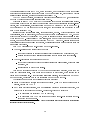
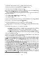
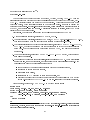
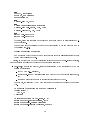
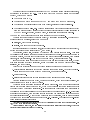
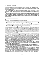
Figure 1: CFSM Specication of a simple system
We will discuss below the analysis tools provided by Polis to check under which conditions event
loss can occur, either by simulation or by formal verication.
Let us consider now a small example of an embedded system, to examine more in detail the
various issues involved.
2.2.1 The seat belt alarm controller
Suppose that we want to specify a simple safety function of an automobile: a seat belt alarm. A
typical specication given to a designer would be:
\Five seconds after the key is turned on, if the belt has not been fastened, an alarm will beep for
ve seconds or until the key is turned o."
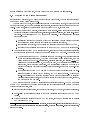
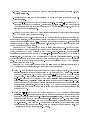
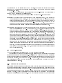
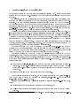
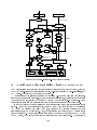
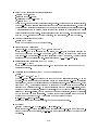
The specication can be represented in a reactive nite state form as shown in Figure 1. Input
events, such as the fact that the key has been turned on or that a 5 second timer has expired, trigger
reactions, such as the starting of the timer or the beeping of the alarm. Stimulus and reaction are
separated by a \/" in the transition labels.
The seat belt controller can be specied to Polis as an Esterel text le as follows:
module belt_control:
input reset, key_on, key_off, belt_on, end_5, end_10;
output alarm : boolean, start_timer;
loop
abort
emit alarm(false);
every key_on do
abort
emit start_timer;
await end_5;
emit alarm(true);
await end_10;
when [key_off or belt_on];
emit alarm(false);
end
when reset
13
end.
The rst two lines declare the input and output signals of the module (CFSM). All input signals
in this case carry only a control information (they are also called pure signals in Esterel), while
the output signal alarm has an associated Boolean value.
The loop statement loops forever. The abort : : : when reset statement executes until the
reset signal is detected, and then is instantaneously killed.8 The every key on do : : : end statement loops, restarting each time key on is detected. Thus the reset signal preempts the abort
statement, while the key on signal preempts the every statement. In fact, all preemptive statements are based on the abort construct. For example, the every key on do ... statement is
equivalent to
loop
await immediate key_on;
abort
...
when key_on
end
Notice the use of await immediate in order to immediately restart the loop when key on is
detected within the statement body. Normally await yields control to the next statement only
when an event on that signal is present in the next transition , after control reaches the awaiting
point.
Each preemptive statement instantaneously kills its body. This means that if both reset and
key on are detected by the CFSM in the same transition (i.e., in the same Esterel instant),
signal start timer is not emitted, and the CFSM is just reset, waiting for key on.
The emit statement can be used to write a value associated with an event (possibly by using a
more complex expression). That value can be read either from a receiving CFSM, using the syntax
?alarm within an expression, or (as in this case) by the environment.
The complete design specication also requires a timer model, that can be represented, assuming
the availability of signal msec (carrying an event once every millisecond), by the following Esterel
specication:
module timer:
constant count_5, count_10:integer;
input msec, start_timer;
output end_5, end_10;
every start_timer do
await count_5 msec;
emit end_5;
await count_10 msec;
emit end_10;
end.
The second line declares symbolic constants (whose actual value will be dened later in the design
ow).
Finally, the await const 5 msec statement counts const 5 (most likely 5000) transitions in
which signal msec has an event, and then yields control to the emit statement, which emits the
corresponding signal.
8
The abort
: : : when
x
command was formerly written as do
14
: : : watching
x
in Esterel.
Esterel is a synchronous language [5, 18]. This means that computation takes (at least
conceptually) zero time . Time elapses only when control reaches a halt or await statement. At
that point, the CFSM transition is completed (including state update and output event emission
for that transition), and the CFSM goes back to its idle condition, waiting for the next set of
events that will wake it up and (possibly, i.e., if they are being explicitly awaited in that idle state)
cause the next transition to occur.
The millisecond timing reference can be generated using either a hardware clock cycle counter,
or using a micro-controller peripheral.
We now suggest creating two text les, called belt control.strl and timer.strl respectively,
containing the controller and timer specications shown above. The Esterel les can be translated
into the SHIFT internal format by using the strl2shift command, as follows:
strl2shift -a belt_control.strl
strl2shift -a timer.strl
The generated SHIFT les can now be input to Polis.
The next design step, after CFSM behavior capture, is functional simulation, to nd and x
bugs.
2.2.2 The Ptolemy co-simulation environment
One of the major problems facing an embedded system designer is the multitude of dierent design options, that often lead to dramatically dierent cost/performance results. Polis oers an
environment to evaluate trade-os via simulation, rather than via mathematical analysis. Hardware/software co-simulation is generally performed with separate simulation models: this makes
trade-o evaluation dicult, because the models must be re-compiled whenever some architectural choice is changed. We use a technique to simulate hardware and software that is almost
cycle-accurate, and uses the same model for both types of components. Only the timing information used for synchronization needs to be changed to modify the hardware/software partition, the
processor choice, or the scheduling policy.
The problems that we must solve include:
fast co-simulation of mixed hardware/software implementations, with accurate synchronization between the two components.
evaluation of dierent processor families and congurations, with dierent speed, memory
size and I/O characteristics.
co-simulation of heterogeneous systems, in which data processing is performed simultaneously
to reactive processing, i.e. in which regular streams of data can be interrupted by urgent
events. Even though our main focus is on reactive, control-dominated systems, we would like
to allow the designer to freely mix the representation, validation and synthesis methods that
best t each particular sub-task.
The basic concept of our co-simulation framework is to use synthesized C code to model all the
components of a system, regardless of their future implementation, starting from an initial specication written in a formal language with a precise semantics, which can be analyzed, optimized
and mapped both to software and hardware.
Software and hardware models are thus executed in the same simulation environment , and
the simulation code is the same that will run on the target processor . Dierent implementation
15
choices are reected in dierent simulation times required to execute each task (one clock cycle
for hardware, a number of cycles depending on the selected target processor for software) and in
dierent execution constraints (concurrency for hardware, mutual exclusion for software). Ecient
synchronized execution of each domain is a key element of any co-simulation methodology aimed
at evaluating potential bottlenecks associated with a given hardware/software partition.
Co-simulation can be done at two levels of abstraction:
Functional : at this level timing is ignored, and the only concern is functional correctness.
Approximate timing : at this level timing is approximated using cycle count estimations for
software, and using a cycle-based simulation for hardware. Even though it is not totally
accurate, this abstraction level oers extremely fast performance. Moreover, it does not
require an accurate model of the target processor, and hence can be used to choose one
without the need to purchase a cycle-accurate model from a vendor.
For co-simulation purposes, Polis is used to generate the C code, but the Ptolemy system
(see [8]) provides the simulator engine and the graphical interface. Co-simulation in the Polis
environment is based on the discrete event (DE) computation model, because it closely matches
the CFSM execution semantics.
Each event occurring in the system (the design and its environment) is tagged by a time of
occurrence. The time must be compatible with:
1. The partial ordering implied by the CFSM specication, meaning that each event that is not
produced by the environment must be the result of some CFSM transition. A transition of
a given CFSM occurs in response to (\is triggered by") a set of events emitted by the environment and/or some CFSM (including a previous transition of the CFSM itself). Emitted
events must have later time stamps than the triggering events.
2. Some estimate of the timing characteristics of the CFSM implementation (e.g, in hardware
or software) within a given execution environment (e.g., processor type or scheduling policy).
This estimate can be unit delay for functional verication in the earliest phases of design.
The creation of the simulation model for the seat belt controller can be done by using the
following commands to the Polis interpreter, after creating the ptolemy sub-directory with the
mkdir ptolemy command. Polis commands can be given to the interpreter after invoking it as
polis from the UNIX shell.
read_shift belt_control.shift
set_impl -s
partition
build_sg
sg_to_c -F -d ptolemy
write_pl -d ptolemy
The command read shift reads in the named SHIFT le and builds the internal data structures.
Help on Polis commands can be obtained using the help command inside Polis. Without arguments it lists the available commands, while with a command name argument it provides brief
usage information.
The commands set impl -s and partition are only required in order to build the appropriate data structures for software synthesis. The C code is synthesized, analyzed (to estimate the
16
execution time of each basic block on a Motorola 68HC11 processor) and written out (including
the timing estimate) with the commands build sg and sg to c.
Finally, the write pl command writes out a le in the Ptolemy model description language,
that species the set of input and output signals in a form understandable by Ptolemy.
Before executing the user interface of Ptolemy we rst need to create the Ptolemy database
that will contain the design and the environment model. This can be done either by hand, or by
using the UNIX command make. We will describe the latter method for the sake of brevity.
Using make to manage the design requires, at the most basic level, creating a le called
Makefile.src in the main design directory (where the Esterel and SHIFT les reside). This
le denes a set of make macros, and is used to build a complete Makefile by the makemakefile
command. In this case, Makefile.src contains just the following lines:
TOP = belt
STRL = belt_control.strl timer.strl
The rst line gives a name to the design, the second line lists the Esterel source les constituting
it.
After executing makemakefile, the command
make ptl
creates the top-level database, named test belt, in the ptolemy subdirectory. It also executes (if
necessary) strl2shift and Polis in order to create the CFSM simulation models (as described
above).
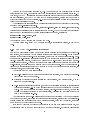
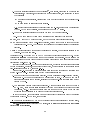
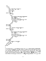
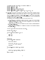
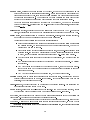
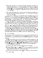
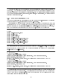
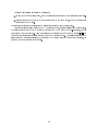
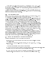
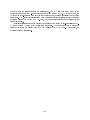
Figure 2 contains a fragment of the synthesized C le for the belt controller. Notice how the
FUZZY macro is used to compute the timing information for each basic block. The arguments to
that macro are \virtual instructions", whose execution time in clock cycles will be computed from
a le modeling the target processor, as described in Section 9.2. The code that will be compiled
and loaded on the target processor will be exactly the same, without the timing information. At
simulation time the executed code accumulates timing information for the chosen processor. The
auxiliary code that is loaded as part of the Ptolemy simulation environment uses that timing
information, together with the user-selected hardware/software partitioning, scheduling policy, and
so on, in order to assign an appropriate time stamp to every simulation event. For hardware
CFSMs the delay for every transition is just 1 time unit, that is 1 clock cycle.
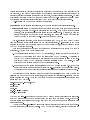
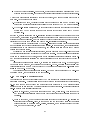
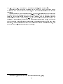
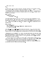
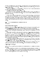
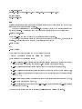
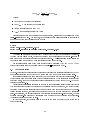
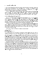
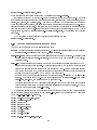
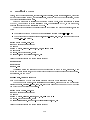
A fragment of the code that denes the interface between the Ptolemy system and the CFSM
C code appears in Figure 3.
Now we are ready to verify the functionality of the design, by interconnecting together the
CFSMs, and providing them with an environment model. The command used to start the user
interface, after executing cd ptolemy, is
pigi belt
The graphical interface requires the creation of an icon for each CFSM. This is accomplished
by the :make-star Ptolemy command (abbreviated as \*"). The command must be typed
with the cursor in the belt window. The \star name" must be belt control and timer in two
successive executions of the command. The \domain" must be DE, and the \star src directory"
must be the complete pathname of the current directory (relative to the user's home directory).
The :open-facet command (abbreviated as \F") can now be used to open the user.pal palette,
in which the CFSM icons have been placed.
Stars (the Ptolemy term for leaf modules, i.e. CFSMs) can be instantiated by:
17
void _t_z_belt_control_0(int proc, int inst)
{
static unsigned_int8bit v__st_tmp;
v__st_tmp = v__st;
startup(proc);
FUZZY(0,"BE+AVV+AVV+AVV+AVV");
/*L1:*/ if (detect_e_reset_to_z_belt_control_0) {
FUZZY(1,"TIDTT+BRA"); goto L4;
}
FUZZY(2,"TIDTF");
...
L3: switch (v__st_tmp) {
case 1: FUZZY(3,"TSDNB"); goto L6;
case 0: FUZZY(4,"TSDNB+TSDNP"); goto L4;
case 3: FUZZY(5,"TSDNB+TSDNP+TSDNP"); goto L14;
default: FUZZY(6,"TSDNB+TSDNP+TSDNP+TSDNP"); goto L7;
}
...
L10: FUZZY(27,"AVC"); v__st = 2; goto L0;
L11: FUZZY(28,"AVV"); v_alarm = 1; goto L12;
L12: FUZZY(29,"AEMIT"); emit_e_alarm(); goto L13;
...
end:
always_cleanup(proc);
return;
}
Figure 2: C code synthesized for the seat belt alarm controller
18
defstar {
name { belt_control }
domain { DE }
derivedfrom { Polis }
desc { Star generated by POLIS
68hc11:
min_time: 142
max_time: 353
tot_size: 478
}
input {
name { e_reset }
type { int }
}
...
output {
name { e_alarm }
type { int }
}
public {
...
/* increment clock count only if SW; cache result of FuzzyDelay */
#define FUZZY(n,d) {if \
((belt_control_Star->needsSharedResource)&& (do_estimate)) {\
_delay += _cache_delay[n]?_cache_delay[n]:(_cache_delay[n]=\
belt_control_Star->FuzzyDelay(d)); }}
...
/* include C code for behavior */
#include "z_belt_control_0.c"
begin {
/* setup code */
...
}
go {
/* transition execution code */
...
_delay = 1.0;
_t_z_belt_control_0(0,0);
end_time = floor( now ) + _delay;
...
}
}
}
Figure 3: Ptolemy interface code for the seat belt alarm controller
19
creating a point in the belt window, by clicking the left mouse button,
moving the cursor above the desired icon in the user.pal window,
typing the command :create (abbreviated as \c").
Icons for primary inputs and primary outputs of the design can be found in the system palette,
available with the :open-palette command (abbreviated as \O").
For this particular design, the user should instantiate the two CFSMs, and enough input and
output arrows to create:
the reset, key on, key off, belt on and msec inputs,
the alarm output.
The primary inputs and outputs must be named, by using the :create command again, as follows:
type the I/O name between double quotes (e.g. "reset"),
execute the :create command with the cursor over the arrow instance.
Finally, instances must be interconnected appropriately. Each interconnection (\net") is created
by:
drawing a path between the CFSM and/or I/O terminals:
{ single-segment paths are drawn by pressing the left mouse button over a previously
created point, dragging the mouse to the end point, and releasing the button.
{ multi-segment paths are drawn by pressing the left mouse button over an end point of a
previously drawn path, dragging the mouse to the end point, and releasing the button.
typing the :create command.
At the end of (and possibly during) the editing session, the netlist displayed in each window can
be saved with the save command (abbreviated as \S").
After the design capture phase is complete, we can begin the functional simulation, by opening
test belt with the :open-facet command. We should now create an icon for belt (a \galaxy"
in Ptolemy terminology) by typing the :make-schematic-icon command (abbreviated as \@")
inside the belt window.
Check, by using the :edit-target command (abbreviated as \T") inside the
window, that the target9 is inherited from the parent.
belt
The belt galaxy should be instantiated in test belt together with stimuli generation and
output display stars from the Ptolemy library. These stars are available in the DE palette (use
the :open-palette command) inside the sources and sinks sub-palettes (use :look-inside, or
\i" over their icons to open them). In this case, we suggest using the TKbutton icon for the inputs
and the TKShowValues icon for the output. These stars can be given useful names by executing
the :edit-params (abbreviated as \e") with the cursor over their instances inside test belt, and
by changing the identifiers and label string parameters respectively.
We will also use a \real-time clock", to drive the msec input of belt, in order to test the
real-time analysis capabilities of Polis. The standard Clock star in the Ptolemy DE palette can
9
See the Ptolemy user's manual for the meaning of the term \target".
20
be used for this purpose, keeping in mind that to get an event every millisecond, the parameter
Interval should be set to 0:001.
The last task before executing the simulation is to select an implementation for each CFSM.
Functional simulation can be done by assigning a unit delay to every CFSM. In order to do this,
execute :edit-params on each CFSM instance in the belt galaxy, and entering the string HW for
the implem parameter. At this stage one must also dene the value of the count 5 and count 10
constants of the timer instance. Their value to get a good \virtual prototype" eect depends on
the speed and the load of the workstation (5000 worked well on a SPARC 20, with the debug
option selected in the run control window to print the current simulation time). The simulation
mechanism also requires the user to choose a CPU for the software partition (even if it is empty)..
This is done by assigning the value 68hc11 to the CPU parameter of belt.
The simulation can be started by executing the :run command (abbreviated as \r") inside the
test belt window, and setting the stop time to a large number, say 1000000. Pushing the buttons
allows the designer to verify that the design behavior matches the informal specication.
After the functional debugging phase is complete, we can now begin dening the architecture
of the design, in terms of partitioning hardware and software, choosing the processor, and so on.
2.2.3 Partitioning and architecture selection
The system architecture, including the software/hardware partition can be dened interactively
within Ptolemy. Suppose that we want to analyze the performance of an all-software implementation, using a Motorola 68HC11 processor. We need to change the implementation of both
CFSMs, by using the :edit-params command, to SW.
The following parameters of test belt should be added (or considered, if they are already
present) now:
1. Clock freq denes the processor clock speed in MHz (for use by the software stars).
2. SCHEDULER denes the real-time scheduling policy to be used for software CFSMs. In this
case, it can be just set to RoundRobin.
3. Firingfile denes the location, relative to the user's home directory, in which a le containing the estimated initial and nal time of each transition of each software CFSM is stored.
4. Overflowfile denes the location, relative to the user's home directory, in which a le
containing the information about lost events is stored. These events correspond, in the realtime software model used by Polis, to missed deadlines .
We can now start the simulation, provide it with a few input events, and then check the
Overflowfile, to analyze missed deadlines. The processor clock speed or the Absclock period
need to be adjusted to make this happen (e.g., deadlines are missed with the clock frequency set
to 1 MHz and the period set to 0.2 msec).
One can also look at the Firingfile, for example using the ptl sched plot utility command,
that displays on a task graph the priority and name of the currently executing CFSM at any point
in time.
Suppose now that we have determined that the real-time constraints cannot be satised on the
chosen processor, unless the timer CFSM is implemented in hardware. We can proceed from here
with the rest of the synthesis procedure.
21
2.2.4 Software and hardware synthesis
Let us save the belt window with the HW implementation for timer and the SW implementation for
belt control. We can now generate a textual version of the Ptolemy netlist with the command
make belt.aux
executed in the main project directory.
The belt.aux netlist le is as follows:
net belt:
input msec , belt_on , key_off , key_on , reset ;
output alarm ;
module timer timer1 [ start_timer/timer1_e_start_timer, msec/msec,
end_5/timer1_e_end_5, end_10/timer1_e_end_10, count_10/5000, count_5/5000 ]
%impl=HW ;
module belt_control belt_control1 [ reset/reset, key_on/key_on,
key_off/key_off, belt_on/belt_on, end_5/timer1_e_end_5,
end_10/timer1_e_end_10, alarm/alarm, start_timer/timer1_e_start_timer ]
%impl=SW ;
.
This textual netlist can also be typed directly by the designer, if the Ptolemy interface is
not available or is too cumbersome for the task at hand and no high-level co-simulation is needed.
Notice how the implementation choice for each CFSM (or hierarchical netlist component, in a more
general case) is specied in the belt.aux le.
After this, we can generate the complete SHIFT netlist of the whole design, by typing
strl2shift belt.aux belt_control.strl timer.strl
Now we can create the sub-directory belt part sg, that will contain the synthesized software,
and synthesize the complete system with the following Polis commands:
read_shift belt.shift
partition
build_sg
set arch 68hc11
set archsuffix e9
read_cost_param
print_cost -s
sg_to_c -d belt_part_sg
gen_os -d belt_part_sg -v 1
connect_parts
net_to_blif -o belt_part.blif
We can now look more in detail at the synthesis commands.
Software synthesis in Polis is based on a Control-Data Flow Graph called S-Graph. The SGraph is considerably simpler than the CDFG used, for example, by a general purpose compiler,
because its purpose is only to specify the transition function of a single CFSM.
An S-Graph hence computes a function from a set of nite-valued variables to a set of nitevalued variables.
22
1. The input variables correspond to input signals10 . Each signal, depending on whether it is a
control signal, a data signal, or it carries both types of information, can correspond to one or
two variables:
(a) a Boolean control variable, yielding true when an event is present for the current transition,
(b) an enumerated or integer subrange variable.
E.g., an input signal representing the current value of a 10-bit counter would be represented
by two S-Graph input variables, one Boolean and one with 210 values.
2. The output variables correspond exactly in the same way to output signals.
An S-Graph is a Directed Acyclic Graph consisting of the following types of nodes:
BEGIN,END are the DAG source and sink, and have one and zero children respectively,
TEST nodes are labeled with a nite-valued function, dened over the set of input and output
variables of the S-Graph. They have as many children as the possible values of the associated
function.
ASSIGN nodes are labeled with an output variable and a function, whose value is assigned to the
variable. They have one child.
Traversing the S-Graph from BEGIN to END computes the function represented by it. Output
variables are initialized to an undened value when beginning the traversal. Output values must
have been assigned a dened value whenever a function depending on them is encountered during
traversal of a well-formed S-Graph.
It should be clear that an S-Graph has a straightforward, ecient implementation as sequential
code on a processor. Moreover, the mapping to binary code, whether directly or via an intermediate
high-level language such as C, is almost 1-to-1.
We use this 1-to-1 mapping to provide accurate estimates of the code size and execution time
of each S-Graph node. This estimation method works satisfactorily if:
1. The cost of each node is accurately analyzed. This is a relatively well-understood problem,
since each S-Graph node corresponds to a basic block of code. Any one of a number of
estimation techniques can be applied, including the benchmark-based cost estimation method
favored by Polis.
2. The interaction between basic blocks is limited. This is approximately true in the case of
an S-Graph, since there is little regularity that even an optimizing compiler can exploit
(no looping, etc.). Also caching performance (for those embedded systems that can take
advantage from it) is likely to be poor in the reactive control domain.
In the Polis system, code cost (size in bytes and time in clock cycles) is computed by analyzing
the structure of each S-Graph node, for example:
the number of children of a TEST node (a dierent timing cost is associated with each child),
States, i.e. signals that are fed back in the CFSM network, can be treated as a pair of input and output signals
for the purpose of this discussion.
10
23
the type of tested expression. For example, a test for event presence must include the RTOS
overhead for event handling, and reading an external value requires to access a driver routine.
A set of cost parameters is associated with every such aspect, and is used to estimate the cost of
each node. Node costs are then used:
1. by printing commands, to display the estimated code size and minimum and maximum execution time (the latter is useful for scheduling) of each software CFSM on a given processor,
2. by the co-simulation environment, to accumulate clock cycles and synchronize the execution
of software CFSMs with each other and with the rest of the system (hardware CFSMs and
environment).
In this way, neither estimation nor co-simulation require the designer to have access to any sort
of model (RTL, instruction set, user's manual) for a processor whose performance he/she wants to
evaluate for a given application. Only the values of the set of parameters (that are part of a library
distributed with Polis for a growing number of micro-controllers) are necessary.
The parameters can be either derived by hand (e.g. inspecting the assembly code after synthesis
and compilation for the target processor) or automatically. In the latter case, the processor library
maintainer needs to compile a set of benchmarks, and analyze their size and timing by using a
proler for the target system.
Obviously a more accurate analysis technique, for example based on a cycle-accurate model of
the processor ([29]) is needed to validate the nal implementation . But the architecture exploration
phase can be carried out much faster, as long as the precision of estimation (currently within 2030% for several processors satisfying the assumptions listed above) is acceptable for the task at
hand.
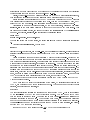
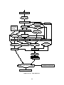
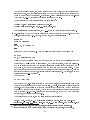
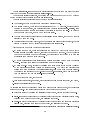
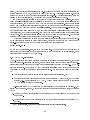
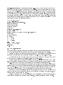
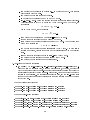
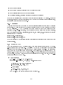
We suggest examining again Figure 2, to identify the various types of S-Graph nodes, and
to compare it with Figure 4, that displays the complete S-Graph. Emission of event alarm with
value false (encoded as 0 on 1 bit) is denoted by the sequence of assignments v alarm = 0 and
alarm = 1 in the S-Graph gure.
The operation of the procedures implementing S-Graphs must be coordinated by a Real-Time
Operating System, that is described in the next section.
2.2.5 The Real-Time Operating System
Cooperation between a set of concurrent tasks (CFSMs in this case) on a single processor requires a
scheduling mechanism. This scheduling for embedded systems must often satisfy timing constraints ,
e.g., on the maximum time between when a given task becomes \ready" (a CFSM receives at least
one input event in this case) and when its execution completes (deadline ). Scheduling policies for
real-time systems are generally classied as:
1. static or pre-runtime , when tasks are executed in a xed, cyclic order. This order may or
may not contain repetitions in order to cope with dierent expected activation times and/or
deadlines.
2. dynamic or runtime , when the order of execution is decided at execution time. Generally the
execution policy is priority-based, in that one among the set of ready tasks is dynamically
chosen according to a priority order . Priority, intuitively, is a measure of \urgency" of each
task, and can be determined, in turn
24
BEGIN
reset
0
1
key_on
1
0
emit start_timer
state
3
2
1
state
3
0
2
1
0
key_off
0
key_off
1
1
0
belt_on
0
belt_on
1
1
0
end_5
0
state = 3
end_10
1
0
1
v_alarm = 1
v_alarm = 0
emit alarm
emit alarm
state = 1
state = 2
END
Figure 4: The S-Graph derived for the seat belt controller
25
(a) statically at compile time, or
(b) dynamically at run time.
Moreover, dynamic scheduling can be
(a) pre-emptive if the currently executing task can be suspended when another task of higher
priority becomes ready,
(b) non-pre-emptive otherwise.
The trade-o, in general terms, is between responsiveness and eciency. Static scheduling, if it
can satisfy the deadlines, is the most ecient mechanism because almost no CPU power is devoted
to computing the schedule at run time (the time that is required to compute the schedule before
execution may not be negligible, but is required only once in the lifetime of a system). On the other
hand, it works satisfactorily only when the time at which tasks become enabled is well-known in
advance. This is the case, for example, for data-ow-oriented systems, in which tasks (data ow
actors) become enabled because of the arrival of input events, which generally arrive in regular
(sampled) streams [25].
On the other hand, if the time of enabling (readiness) of tasks is unpredictable, as is the case for
the control-dominated targeted by Polis, such a scheme may be too inecient. Static scheduling
requires execution of a task whenever it is expected to be ready , or at least to cyclically test it for
readiness . If enabling times are not predictable, then too much CPU power becomes wasted in
simply polling events that are unlikely to occur. In that case, dynamic scheduling may become
necessary to use the CPU power better (executing the tasks rather than checking which one is
ready).
Moreover, verifying if a given scheduling satises all the deadlines is an extremely hard problem,
even for the simple policies outlined above and assuming that all tasks require a xed execution time.
Hence, real-time systems theory has developed a broad choice of conservative analysis methods.
Such methods can guarantee that a set of tasks will never miss a deadline, given:
upper bounds on the execution times of each task,
lower bounds on the task activation intervals,
deadlines,
possibly other information used to rene this simple model, such as
{ dependencies between task activations,
{ context swapping overhead (for pre-emptive scheduling),
{ a set of tasks with \soft deadlines" that must be served in the \background"11,
a particular scheduling policy (task ordering, priority assignment, : : : ).
The maximum processor usage that guarantees schedulability in the presence of irregular activation of tasks is about 60% for pre-emptive static-priority dynamic scheduling using the Rate
Monotonic priority assignment algorithm ([26]), but much lower for static scheduling. Hence the
choice of scheduling algorithm must carefully consider the real-time characteristics of the system
at hand.
A deadline is hard if missing it leads to a system failure, and must be absolutely avoided. A deadline is soft if
missing it has just an associated cost, that must generally be minimized over time.
11
26
Polis provides both conservative analysis techniques (based on classical real-time theory results,
summarized e.g. in [17]) and the estimated timing simulation technique described above, in order
to choose the scheduling policy for a given system.
The Real-Time Operating System synthesis command in Polis is called gen os. Its purpose is
three-fold:
1. It assigns I/O ports (using port-based or memory-mapped I/O) to signals exchanged between
software CFSMs and the rest of the world (environment and hardware CFSMs).
2. It schedules the CFSMs, by assigning a priority to each one of them, based on user-dened
periods and deadlines, and estimated maximum execution times (obtained as the longest
timing path in each S-Graph).
3. It generates a C program that implements the I/O drivers and schedules the CFSMs appropriately. The same C program can also be compiled and run on a workstation for debugging
purposes.
The operation of the RTOS is as follows:
each control signal buer is implemented as a single bit in a memory location for each CFSM
input (one such set of bits for each CFSM).
each data signal buer is implemented in a single memory location for each CFSM output
(of the appropriate type to contain at least its integer subrange).
event emission is implemented as a table-driven routine that sets the presence bits for all
receiving CFSMs.
event detection is implemented as a macro that tests the bit.
event consumption is implemented as a \cleanup" function that is called at the end of each
S-Graph execution (Figure 2).
input events from outside the software partition can be implemented
{ either as Interrupt Service Routines (ISRs), that simply call the corresponding emit
routine,
{ or as polling, by a special polling task that is scheduled periodically, tests the appropriate
input port bit, and calls the emit routine.
output events to the external world are implemented by the emit routine, by toggling the
corresponding output port bit.
All macros and routines that implement event handling are dened by the RTOS code and executed
and called by the code synthesized from the S-Graph.
The scheduler rst calls each CFSM once to initialize its internal state and to emit initial events
(if any). Then it loops forever, scheduling CFSMs whenever they have input events and according
to the appropriate priorities. Pre-emptive scheduling is implemented by allowing the event delivery
routine to call a CFSM with a higher priority than the one that is currently executing.
The atomicity of CFSM transitions is guaranteed by a double-buering of state signal presence
bits and input signal value buers that are copied at each CFSM invocation from the global copy.
See, for example, the buering of v st in Figure 2.
The commands
27
set arch 68hc11
set archsuffix e9
inform Polis about the type of processor by setting two internal variables. The former denes
the processor family that determines, for example, the instruction set architecture and hence the
set of code cost estimation parameters. The latter denes the specic member of the family, that
determines, for example, the on-chip peripherals, the I/O conguration, and the memory map.
Details about the memory map and I/O port locations and directions are given to Polis by means
of processor conguration les.
The next two commands in the sample synthesis session deal with interface and hardware
synthesis.
2.2.6 Interface and Hardware Synthesis
Polis assumes a standard event communication mechanism over the various possible interfaces:
1. Software to software interfaces are implemented by the RTOS as described above.
2. Hardware to hardware and hardware to environment interfaces use a wire to carry the event
presence information, and a set of wires to carry the event value. The event presence bit is
held high for exactly one clock cycle to signal the presence of an event. No latching or other
overhead is required, since hardware CFSMs are executing one transition per clock cycle,
and all their outputs are latched for one cycle by the synthesis procedure described below.
3. Environment to software and hardware to software interfaces use a request-acknowledge protocol to make sure that the event is received by the RTOS (not by the CFSM, since responsiveness to individual events is not guaranteed by Polis), similar to the classical polling or
interrupt acknowledge mechanism. The hardware side of the interface is implemented by a
simple synchronous set/reset ip-op.
4. Environment to hardware, software to environment and software to hardware interfaces use
an edge detector (optional in the environment to hardware case) to translate a pulse (that can
potentially last more than one clock cycle) to the \one cycle per event" hardware protocol.
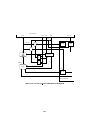
Figure 5 shows the circuit implementation and timing diagrams of the software to hardware,
and hardware to software interfaces.
Interface synthesis also handles memory-mapped and port-based I/O transparently to the user.
It assumes that the memory address bus of the processor is accessible, and uses a library of
processor-dependent interface modules to adapt the protocol. Memory-mapped addressing involves
the synthesis of address decoders both for software to hardware and hardware to software interfaces. Addresses assigned by the RTOS are automatically used by the synthesized interfaces, and
displayed to the user for hardware debugging purposes.
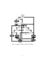
Figure 6 shows a schematic view of the interfacing mechanism. The I/O assignment for this
specic example is printed out by the gen os command, and is as follows:
EVENT
EVENT
...
EVENT
- VAR
{ 1} *reset INP-VIRT: PORT_0E<1> ACK: PORT_0A<16>
{ 2} *key_on INP-VIRT: PORT_0E<2> ACK: PORT_0A<32>
{ 8} *timer1_e_start_timer OUT: PORT_0D<8>
{ 0} belt_control1_e_alarm [1 bytes] (RAM)
28
HW
SW
x
x
y
x
Y
y
0/0
1/0
0/0
0
x
1
D
y
Q
1/1
ack
HW
SW
x
y
x
Y
ack
x ack
0−/0
11/0
y
−1/0
0
−0/1
1
x
D
Q
10/1
y
ack
Figure 5: The hardware/software interface buers
29
microcontroller
Dbus
Abus
R/W
ADDRESS
Eclk
Port A
CK
IDATA
SW-HW
SW-HW
En
En
OE
DEC.
micro.blif
DEC.
WE
ODATA
MUX
Ack
OE_INT
HW-SW
Custom hardware
Figure 6: The hardware/software interfacing logic
It means that input event reset is assigned to bit 1 of port E of the 68hc11, while its acknowledge
output is assigned to bit 4 of port A.
Hardware synthesis creates a Moore machine for each CFSM. All output control and data signals
are latched. This unit delay is compatible with the CFSM model, and ensures safe composability.
Logic synthesis can then be used to optimize the circuit. For rapid prototyping purposes, Polis
provides a path to implementation using XILINX FPGAs, by producing the output netlist in the
XNF format.
Other output logic netlist formats include BLIF, Verilog and VHDL (the latter two use a very
simple technology-independent basic gate library). See the documentation of SIS [31] for more
information about logic optimization, technology mapping and library description formats.
This concludes the short presentation of the capabilities of Polis.
30
3 The Polis design methodology
This section describes how the Polis design methodology is organized, and shows how the designer
can manage the design les through the various synthesis and validation steps.
3.1 Overview of the design ow
The Polis design ow is illustrated in Figure 7. The main steps are as follows:
1. High Level Language Translation Designers write their specications using some high
level language that must have an Extended Finite State Machine semantics. Examples of
such languages are Esterel [5] (used for most of the examples in this manual, Section 5.1),
StateCharts [16], and the synthesizable subsets of of Verilog or VHDL. Esterel source les
are characterized by an extension .strl.
The translator from Esterel, called strl2shift, receives as input the .strl les describing the CFSM behavior, as well as some auxiliary information (such as type and constant
denitions, and the CFSM netlist) contained in a le with extension .aux. It produces a
set of les in the SHIFT format (Section 14) describing both the individual CFSMs (with
extension .cfsm), and the complete system (with extension .shift).
2. System Co-simulation This step is used in a closed loop with system partitioning and
depends on software synthesis for the generation of the executable models and the clock cycle
estimates. It can be done either using the public-domain Ptolemy simulator ([8]) or using
any VHDL simulator, as described more in detail in Section 6.
3. Formal Verication The formal specication and synthesis methodology embedded within
Polis makes it possible to interface directly with existing formal verication algorithms that
are based on FSMs. Polis includes a translator, described in Section 8, from CFSMs to
classical Finite State Machines, which can be fed directly to verication systems ([2]).
4. Design Partitioning Design partitioning is the process of choosing a software or hardware
implementation for each CFSM in the system specication. A key point of this methodology
is that the CFSM specication is implementation-independent, thus allowing the designer
to interactively explore a number of implementation options. Partitioning is done using the
same user interface as co-simulation, thus allowing a tight interaction between architectural
choices and performance and cost analysis.
5. Software Synthesis A CFSM sub-network chosen for software implementation is mapped
into a software structure that includes a procedure for each CFSM, together with a simple
Real-Time Operating System:
(a) CFSMs. The reactive behavior is synthesized in a two-step process (Section 9):
Implement and optimize the desired behavior in a high-level, processor-independent
representation of the decision process similar to a control/data ow graph.
Translate the control/data ow graph into portable C code and use any available
compiler to implement and optimize it in a specic, micro-controller-dependent instruction set.
31
Formal Languages
Translators
System Behavior
Co−Simulation
Scheduler
Template +
Timing
Constraints
SW Synthesis
S−Graph
OS Synthesis
Partitioning
Estimates
Formal
Verification
Partitioned Specification
Interface
Synthesis
HW Synthesis
HW Interfaces
Unoptimized HW
Task Synthesis
Logic Synthesis
Verif. Interm. Format
Hw Estimation
Sw Estimation
Optmized HW
C−code
Partitioning
Optmized HW
BOARD LEVEL PROTOTYPING
Physical Prototype
Figure 7: The Polis design ow
32
Standard Components
This methodology results in better optimization and tighter control of software size and
timing than with a general-purpose compiler. A timing estimator quickly analyzes the
program and reports code size and speed characteristics (Section 9.2).
The estimator is a key component of our co-simulation methodology, because it provides
accurate estimates of program execution times on any characterized target processor, by:
i. appending to each statement in the C code generated from the control/data ow
graph instructions that accumulate clock cycles,
ii. compiling and executing the software on the host workstation.
(b) Real-Time Operating System (Section 10). An application-specic OS, consisting of a
scheduler and I/O drivers, is generated for each partitioned design. Currently POLIS
allows the designer to choose from a set of classical scheduling algorithms (e.g. RateMonotonic and Deadline-Monotonic, [27]).
Interfaces between dierent implementation domains (hardware-software) are automatically synthesized by Polis as part of the RTOS and hardware synthesis tasks. These
interfaces come in the form of cooperating circuits and software procedures (I/O drivers)
embedded in the synthesized implementation.
6. Hardware Synthesis A CFSM sub-network chosen for hardware implementation is directly
mapped, as described in Section 11, into an abstract hardware description format. This format
can be BLIF (les with extension .blif, [31]), VHDL (les with extension .vhd) or XNF (les
with extension .xnf, for implementation on Field Programmable Gate Arrays), as described
in Section 11.
7. Rapid Prototyping One of the major advantages of a unied co-design methodology is the
ability to exploit automated synthesis techniques to quickly obtain a physical prototype of
the system, to be deployed in the eld, as described in Section 12.
3.2 Managing the design ow
Currently the design ow in Polis can be managed using the UNIX tool make. We hence assume
that the reader is familiar with the basic functions and features of make.
Both the input language translation process, and the following synthesis steps, are controlled
by creating a le called Makefile.src, containing only make macros and project-dependent compilation commands. All the other targets, dependencies and so on are automatically derived from
a set of skeletal les contained in the Polis library. The actual Makefile is created, starting from
Makefile.src, as follows:
the rst time, by typing the command makemakefile.
afterwards, by typing the command make makefile, that automatically checks if Makefile.src
or the library skeleta have been changed.
For the specication step, the designer can specify the following macros (see, e.g., the Makefile.src
in the dashboard example directory described in Section 4):
STRL listing the Esterel source les that are part of the design specication .
SHIFT listing the hand-written SHIFT (i.e., excluding those compiled from Esterel sources)
source les that are part of the design specication .
33
OTHERSTRL listing any other Esterel source les required for the Ptolemy simulation.
TOP giving a name to the project. This name is used to implicitly dene the name of several les
and directories used by Polis:
1. $(TOP).aux is the main netlist specication le, either written by hand (if Ptolemy is
not used) or derived as described in Section 6.1 from the graphical netlist created using
pigi.
2. $(TOP).shift is the complete system netlist, generated by strl2shift from the auxiliary le and the Esterel and SHIFT leaf les.
3. $(TOP)_sg and $(TOP)_part_sg are the directories where the synthesized software for
an all-software and a mixed hardware/software implementation respectively will be put
(as described in Section 9).
4. $(TOP)_part.blif is the le where the BLIF netlist produced by the hardware synthesis
step will be put (as described in Section 11).
INIT AUX listing an optional type and constant denition le for strl2shift. This le is used
directly for the rst execution of strl2shift (creating the Ptolemy simulation models, as
described in Section 6.1), and is prepended to the netlist generated from the Ptolemy netlist
by ptl2shift (Section 6.1.4).
Note that if the designer uses make to manage the project, then
the name of the project (macro TOP) must be dierent from that of any Esterel or SHIFT
source le,
each Esterel le can contain only one module (this is a good idea anyway: : : ), that is
translated into a single CFSM, one
the name of each Esterel module must be the same (including the case) as that of the
Esterel source le containing it (with .strl appended).
Otherwise, the designer is responsible for keeping track of the dependencies and name correspondences assumed and used by Ptolemy and Polis. We recommend using make, at least at the
beginning, in order to become familiar with those assumptions.
Other useful macros that can be re-assigned in Makefile.src to alter the default behavior of
make are:
OCT2SHIFT denes the command used to translate the Ptolemy netlist into an auxiliary netlist
le for strl2shift.
INT denes the number of values used to translate the Esterel integer data type in SHIFT.
ESTERELHOME denes the location where the ocial Esterel distribution is installed (if it
is installed at all).
STRLCOMP denes the command used to invoke the ocial Esterel compiler, e.g. by the
strl2shift command.
POLISCOMP denes the command used to invoke the Polis compiler.
STRLFLAGS is the set of compilation ags that are passed to the Esterel compiler.
34
S2SFLAGS is the set of compilation ags that are passed to the strl2shift translator.
HW MOD can be dened in Makefile.src to implement a specic set of CFSMs in hard-
ware, overriding the partition dened in the SHIFT le (if any). It must take the form -h
cfsm or net name ..., and if a net instance name is given, the implementation is propagated
to all the CFSMs within it.
SW MOD can be dened in Makefile.src to implement a specic set of CFSMs in software,
overriding the partition dened in the SHIFT le (if any). It must take the form -s
cfsm or net name ....
SETATTR can be dened to add some design-specic attributes to hierarchical objects (nets or
CFSMs), using the set attr command (see the help page).
SETSWATTR can be dened to add some design-specic attributes to the software partition,
using the set sw attr command (see the help page and Section 10).
POLISLIBS can be dened to add some user-written C les to the software partition, e.g. to
implement some functions called by CFSMs that will certainly be implemented in software.
STRLLIBS can be dened to add some user-written C les to the list of les used by the Esterel
simulation (by default it is the same as POLISLIBS).
CLEAN can contain a list of les that must be deleted when the make clean command is executed, to remove all outputs of the compilation process. Use it carefully, because it can be
dangerous: : :
UC denes the micro-controller family that will be used. The macro UCSUFFIX can then be
used to further identify a member of the family, by concatenation with UC.
Generally speaking, the UC macro (used for software cost estimation and stored in the arch
polis variable) should identify the instruction set, while the UCSUFFIX macro (used by
the RTOS and interface generation commands and stored in the archsuffix polis variable)
should identify the bus and memory architecture.
For example,
UC = 68hc11
UCSUFFIX = e9
is the default value of the macros, identifying the 68hc11e9 variant of the Motorola 68hc11
family.
ISSUC can contain the name of a micro-controller (by default UC is used) to be used when
performing co-simulation with an Instruction Set Simulator, as described in Section 6.5. The
macro (no longer used for other purposes, since version 0.4 of Polis) must be in the form:
ISSUC = -a name
35
4 A medium-size design example
The medium size example that we will use for the rest of the manual is a dashboard controller. It
is not a \real design" in a strict sense, but it includes most of the functionality of the embedded
system that controls a real car dashboard. It has the following inputs:
RESET initializes everything.
KEY and BELT inform the dashboard controller about the status of the ignition key (on or
o) and of the seat belt (fastened or not).
ECLK is the micro-controller clock, which is used by the timer unit to provide a timing
reference.
WHEEL PULSE is emitted by a sensor 4 times for each wheel revolution.
ENGINE PULSE is emitted by a sensor 4 times for each engine revolution.
FUEL LEVEL informs the dashboard controller about the level of the fuel in the tank.
WATER LEVEL informs the dashboard controller about the temperature of the water in the
engine.
PARTIAL RESET initializes the partial kilometers counter.
It has the following outputs:
BELT ALARM HW controls the seat belt alarm buzzer and light.
TOTAL TENTH KM RUN and PARTIAL TENTH KM RUN display the total and partial
traveled distance.
FUEL ALARM HW signals a low fuel condition.
WATER ALARM HW signals a high water temperature condition.
ENGINE COIL 0, ENGINE COIL 1, SPEED COIL 2 and SPEED COIL 3 are PWM-coded
signals that drive the coils of the wheel and engine speed display instruments (2 signals for
each coil, 2 coils for each instrument).
The complete example is contained in the directory
$POLIS/examples/demo/dac_demo
In order to see the hierarchy, change your current directory to
$POLIS/examples/demo/dac_demo
and execute the command
make ptl
in order to create the simulation models from the Esterel source les. Then change the directory
to
$POLIS/examples/demo/dac_demo/ptolemy
36
and execute the following command12 :
pigi test_dac_demo
The components on the left hand side (TkButtons, TkSlider, Impulse, FREQ GEN ) are the
signal generators which drive the dashboard controller; the ones on the right (TkShowValue, MEASURE DC, Myxyplot ) display the output of the computation. These blocks are not part of the
dashboard design, which is entirely enclosed in the dashboard galaxy. In order to display the
contents of intermediate- and leaf-level hierarchical units, called galaxies and stars respectively in
Ptolemy, go over their icons and type \i". Galaxies are displayed as netlists, stars (CFSMs) are
displayed as Esterel source les.
Functionally, the dashboard is composed of the following main groups of CFSMs:
1. A timing reference generator, including CFSMs frc, pwmfrc .
2. The seat belt alarm controller, including CFSMs belt, DEBOUNCE, oc2 prog rel and LATCH HW ,
that sounds an alarm when the seat belt is not fastened at engine start-up time.
3. The fuel level indicator and water temperature indicator, including CFSMs ALARM COMPARE,
LATCH HW , that output an alarm when the tank is almost empty or the water temperature
is too high. The two values are computed using the same CFSM, and only some constants
are changed.
4. The odometer indicator, including CFSMs ODO COUNT PULSES and ic1 , that counts and
normalizes wheel pulses.
5. The engine and wheel speed gauge controllers, including all other CFSMs. The two controllers
are very similar, though not identical, and dier mainly in the normalizations constant. Each
controller is composed of a hierarchical subunit that:
computes speed by counting pulses occurring between two reference times,
averages it to reduce the eect of noise,
normalizes it for display,
splits it into an X/Y pair used to drive the gauge coils, and
produces the Pulse Width Modulated outputs for each of the four coils (the PWM output
is then de-modulated by MEASURE DC in the top-level galaxy for display purposes).
Let us consider, for example, CFSM BELT . The Esterel source le is:
module BELT:
input RESET, KEY_ON, KEY_OFF, BELT_ON, OC2_END;
output OC2_START : integer, ALARM : boolean;
constant CONST_ALARM_OFF : boolean, CONST_MAX_FRC_NUMBER : integer,
CONST_PRE_SCAL_5 : integer, CONST_PRE_SCAL_10 : integer;
var
SCALER : integer
in
The reference manual of the pigi editor is part of the Ptolemy documentation. Section 6.1 contains a short list
of commands. Moreover, you may need to use the command polis pigi test dac demo instead if your shell does
not dene the PWD environment variable.
12
37
loop
abort
loop
emit ALARM(CONST_ALARM_OFF);
SCALER := 0;
await KEY_ON;
abort
signal DONE_5 in
weak abort
loop
emit OC2_START(CONST_MAX_FRC_NUMBER);
await OC2_END;
SCALER := SCALER + 1;
if (SCALER = CONST_PRE_SCAL_5) then
SCALER := 0;
emit DONE_5;
end;
end;
when DONE_5
end signal;
end;
emit ALARM(not CONST_ALARM_OFF);
signal DONE_10 in
weak abort
loop
emit OC2_START(CONST_MAX_FRC_NUMBER);
await OC2_END;
SCALER := SCALER + 1;
if (SCALER = CONST_PRE_SCAL_10) then
emit DONE_10;
end;
end;
when DONE_10
end signal;
when [KEY_OFF or BELT_ON];
end loop
when RESET;
end loop
end var
.
The behavior of the CFSM is as follows. Every time the RESET signal is present, it is reinitialized
by the outermost abort{when statement enclosed in a loop (this is typical of reactive systems,
which maintain a permanent interaction with the environment, and hence need such a loop). During normal operation, it waits for the KEY ON signal, requests the oc2 prog rel CFSM to start
counting, waits for 5 seconds (as signaled by the OC2 END signal from the timer), emits ALARM ,
waits for another 5 seconds, and switches o ALARM . It is reset, initializing ALARM , any time
38
KEY OFF or BELT ON are detected by the innermost abort{when statement13.
We suggest that the reader have a brief look at the other CFSMs now, in order to become
familiar with the Esterel syntax and semantics, and with the overall operation of the dashboard
controller.
Note: as described more in detail in Section 6.1.2, the micro-controller timer can be simulated
at various levels of abstraction. This means that there is a need to vary the frequency of the clock
driving it. If the chosen implementation of the timer is BEHAV, then the simulation parameter
SIMSCALE should be set to a high value, e.g., 25, in order to produce a single clock pulse at the
beginning of the simulation, to \kick o" the behavioral (abstract) timer model. On the other
hand, if the chosen implementation or the timer is HW, then SIMSCALE should be set to a low value,
like 4 or 5, in order to simulate one every 24 or 25 \real" clock cycles (with SIMSCALE set to 0, you
get a very slow cycle-accurate simulation of the timer).
13
The weak
abort
: : : when
statement was formerly written as trap
39
NAME in
.
: : : end
5 Specication languages
This section describes the currently supported specication languages for Polis. It is being continuously updated, as new languages are added to the system.
Note that the overall modeling philosophy implied by the Polis system is somewhat peculiar,
with both advantages and disadvantages with respect to other digital and embedded system design
methods. In particular, the CFSM model that is at the basis of Polis [12] is designed so as
to put the least constraint on the implementation, while still maintaining a reasonable control
over the performance and behavior of the implementation, as well as over the synthesis process.
The main goal of the project was to achieve comparable cost and performance to a good manual
implementation for hardware, software and interface components. This could not obviously be
achieved while maintaining complete equivalence of behavior between the specication and the
various styles of implementation, unless a very vague meaning is given to the term \behavior". The
CFSM model uses a locally synchronous, globally asynchronous paradigm, that
determines exactly how a module (CFSM) behaves whenever it performs a transition, but
poses little restriction on the speed of communication between modules or on the relative
timing of module executions (the \scheduling policy").
The designer should not expect that the behavior of a high-level untimed or even timed cosimulation performed as described in 6.1 will be directly and easily comparable with that of a
detailed cycle-accurate co-simulation of the hardware, together with the software running on a
processor model. Even dierent compilation options, triggering dierent optimization algorithms,
may provide implementation behaviors that have dierent timing characteristics. The purpose of
high-level co-simulation is to provide the designer with a exible environment in which architectural
trade-os can be explored. Precise validation of the nal implementation should be done with a
much more accurate model (e.g. a cycle-accurate processor model and a hardware simulator [29]).
Both the simulation testbench and the formal properties used to validate the specication should
be chosen with these considerations in mind. In particular, any attempt to compare specication
and implementation, based on exact timing data has little chance of success (except perhaps in the
case of a fully-hardware implementation). On the other hand, relative timing, \causality" links,
and satisfaction of constraints like \faster than" or \slower than" can be checked at all levels of
abstraction, and are preserved by the synthesis steps.
5.1 The strl2shift translator
Esterel is the recommended specication language for Polis. Its clean syntax and semantics
make it well-suited for co-design of control-dominated embedded systems.
Translation from Esterel to SHIFT is performed by a program called strl2shift. This in
turn calls the ocial Esterel compiler ([14]), followed by a translator, called oc2shift, from an
output format of the Esterel compiler to SHIFT (Section 14). We recommend that Polis users
obtain a license for the Esterel compiler by sending e-mail to [email protected], or
by looking at the WEB page
http://www.inria.fr/meije/esterel
because it oers an excellent functional debugging environment. Moreover, the combination of
Polis, Esterel and oc2shift oers some very nice capabilities, like CFSM collapsing. oc2shift
40
currently supports version 5 of the OC intermediate format generated by the esterel, lustre and
signal compilers14 . Other versions will be added as appropriate.
The command format is:
strl2shift [option ...] [aux_file] [esterel_file ...] [shift_file ...]
The command takes as input a set of les including:
1. Any number (including zero) of Esterel source les, characterized by the extension .strl.
These les are compiled using either the esterel and oc2shift programs.
2. Any number (including zero) of SHIFT source les, characterized by the extensions .shift
or .cfsm. The former identies user-written SHIFT les or the result of previous strl2shift
partial compilations of lower levels of a complex hierarchical netlist. The latter identies leaf
CFSMs produced by oc2shift, as the result of a previous compilation using the -c or -C
option of strl2shift (see below).
3. At most one auxiliary le, characterized by the extension .aux, that can specify the following
information in order
signal and variable type-related information (denition of Esterel types, re-denition
of integer signals and variables, denition of unsynchronized signals),
denition of the value of constants,
creation of a hierarchical netlist, by instantiating and interconnecting the CFSMs specied by the Esterel and SHIFT les.
Let us consider each component of the auxiliary le in order (note that constant and type
denitions must precede the netlists):
Denitions of user-dened types declared in the Esterel modules. Esterel allows the
designer to declare such types, but their denition must be external. Suppose, for example,
that declarations like
type
type
type
type
rgy;
int8bit;
uint8bit;
float;
occur in one of the Esterel source les. Then the following lines in the auxiliary le can
dene those types:
typedef
typedef
typedef
typedef
14
enum { red, green, yellow } rgy
mv 128 int8bit
nb unsigned 8 uint8bit
nb 31 float
Testing with lustre and signal, however, has been limited so far.
41
The rst type is enumerated, the second is signed and ts in 8 bits, the third is unsigned and
also ts in 8 bits. The last declaration informs POLIS that the \float" type is signed and
ts in 32 bits (31 plus 1 for the sign). See Section 5.2 for a discussion about how non-integer
types (such as, e.g., type float) are partially supported by Polis.
The general syntax of the typedef statement is as follows15 :
typedef {nb,mv} [unsigned] <number> <type_id>
typedef enum '{' <sym_id> [',' ...] '}' <type_id>
where <number> is a positive integer, and <..._id> is any valid alphanumeric identier.
Re-declaration of Esterel integer variables as integer subranges or as user-dened types
(again, see also Section 5.2). Suppose, for example, that declarations like:
module m:
input a: integer;
...
var b, c, d: integer in
...
occur in an Esterel source le. Then the following statements in the auxiliary le
mv a 128
mv b, c unsigned 256 in m
specify that those variables don't have the default number of bits for the integer data type
(as specied by the -i option of strl2shift), but 8 bits (a is signed, while b is unsigned).
The in m clause species that the subrange declaration applies only to variables b and c
of module m, not to any other variable with the same name in the whole design. The nb
statement denes the number of bits that the variable can take (plus one if signed), while the
mv statement denes the number of values (positive values if signed). Of course, nb is to be
preferred for power-of-two ranges16.
The statement
nb d 31 float in m
on the other hand, re-declares variable d to be of type float, and simultaneously tells Polis
that this type requires 32 bits (31 plus 1 for the sign). This re-declaration of integer variables
as user-dened types is allowed in order to be able to use the standard Esterel arithmetic
operators on oating point variables, but can lead to compilation or runtime errors later if
used improperly (e.g. if the re-declared type is not numeric, or if the CFSM is implemented
in hardware, as described in Section 5.2).
The general syntax of the nb, mv and enum statements is as follows:
{nb,mv} <var_id> [',' ...] [unsigned] <number> [<type_id>] [in <mod_id>]
enum <var_id> [',' ...] '{' <sym_id> [',' ...] '}' [<type_id>] [in <mod_id>]
15
16
A list in braces denotes choice, dots denote repetition, and square brackets denote an optional part.
Note that the statement nb a 7 in fact denes a as an 8 bit variable (7 for the value, 1 for the sign).
42
Re-declaration of Esterel signals as pure values 17, without the control information, by using
the following syntax (assuming that the same declarations as in the previous case occur in
the Esterel le):
value a
species that signal a is actually a pure value, that cannot be awaited or watched . This is
especially useful for hardware CFSMs, because it saves one wire, otherwise used to indicate
the presence of an signal.
The general syntax of the value statement is as follows:
value <var_id> [',' ...] [in <module_id>]
Denition of the value of Esterel constants, using one of two mechanisms:
1. a define statement, like:
define TIME_SPEED 1000
2. the parameter passing mechanism described below.
The latter form is recommended for constants whose value is subject to change (like scaling
factors, clock division factors, lter coecients and so on), because the Ptolemy simulation
environment allows the user to dynamically change them at simulation time only if they don't
appear in a define statement. \True" constants, like a xed-point approximation of (recall
that Esterel directly supports only integers), on the other hand, can be handily dened
using the define statement.
Note that the parameter passing denition does not require any user action at this stage (only
the declaration of constants in the Esterel les). Appropriate parameter declarations for
Ptolemy are inserted automatically by strl2shift and by polis.
The general syntax of the define statement is as follows:
define <const_id> <number> [in <module_id>]
Creation of a hierarchical netlist, by instantiating and interconnecting the CFSMs specied
by the Esterel and SHIFT les. This interconnection is specied using a syntax that is
reminiscent of the Esterel copymodule statement, as follows. Suppose that the following
module was declared in Esterel:
module example:
input i(integer);
output o(integer), done;
constant norm;
...
17
The Esterel sensor data type serves an equivalent purpose for input signals, but it cannot be used for output
signals.
43
Then the following netlist describes two cascaded instances of example , called ex1 and ex2
respectively. Note that internal interconnection signals like o1 to i2 need not be declared
(but the types of the interconnected signals must match).
net two_examples:
input i1;
output o2, done1, done2;
module example ex1 [i/i1, o/o1_to_i2, done/done1, norm/125];
module example ex2 [i/o1_to_i2, o/o2, done/done2, norm/250];
.
Note the nal \." and the constant denition mechanism. Formal/actual matching is done
by name (hence the order of parameters is not signicant), and newlines can be used as white
space in the net section (while they are line terminators for typedef and define statements).
Any number (including zero) of net sections can appear in an auxiliary le, to describe a
complex hierarchical netlist. Instantiated modules can be either leaf modules or other nets
dened in the auxiliary le. The rst net is by convention the top level in the hierarchy.
Instance names can be explicitly given, as in this case (ex1, ex2) or be automatically assigned
by strl2shift as the model name followed by a unique integer (they would be example 1,
example 2 in this case).
SHIFT attributes, dening for example the implementation of each CFSM or hierarchical
unit, can be specied as part of each module statement. See also Sections 14 for a list of
currently supported attributes and 6.1 for the implementation specication mechanism. In
the example above, a hardware or software implementation for the two instances could be
specied as follows:
...
module example ex1 [i/i1, o/o1_to_i2, done/done1,
norm/125] %impl=HW;
module example ex2 [i/o1_to_i2, o/o2, done/done2,
norm/250] %impl=SW;
.
The general syntax of the net,
input, output
and module statements is as follows:
net <net_id> ':'
input <signal_id> [',' ...] ';'
output <signal_id> [',' ...] ';'
module <cfsm_or_net_id> <inst_id> '[' <form_param_id> '/' <act_param_id>
[',' ...] ']' [<attr_id> '=' <attr_value> [',' ...]] ';'
...
'.'
The options are as follows:
-a compiles each Esterel le into an individual SHIFT le, without requiring an auxiliary le.
-c compiles each Esterel le into an individual SHIFT le, while considering only the type and
constant denition statements of the auxiliary le.
44
-C compiles all Esterel les into a single SHIFT le, while considering only the type and constant
denition statements of the auxiliary le.
5.2 Support for user-dened data types
Polis currently oers some support for user-dened data types, limited to software implementation
and to pure assignment (e.g., copying through interfaces) in case of hardware implementation.
There are two separate cases to consider.
1. The rst is numeric non-integer (i.e. oating point) types. In that case, the easiest mechanism
is to declare variables and signals18 that will later be re-dened as oating point as integers in
Esterel, thus relying on implicit conversions provided by the C compiler for the generated
code.
The re-denition is carried out in the auxiliary le, by using the <type_id> eld in the nb
statement, as follows:
nb <var_id> [',' ...] <number> {float,double} [in <module_id>]
It is strongly recommended to specify the same number of bits (plus one for the sign) for the
float or double type as implied by the target C compiler, because that is the number of
bits used, e.g., to instantiate buers in the hardware/software interfaces. This is required to
ensure correct operation if, for example, a small hardware CFSM performing the function of
a latch is used to make an input or an output to the software partition \permanent" (e.g. if
memory-mapped I/O is used, as described in Sections 10 and 11).
There is no other action required at the Esterel level in this case.
2. The second case is when the type is a C structure or union. In that case, the Esterel type
construct must be used, and appropriate routines to get and set the value of each eld of the
structure must be declared in each Esterel le.
For example, let us consider the denition of a two-integer structure used to store complex
numbers with integer-valued real and imaginary parts. In this case, at the very least one
should use the following statements at the beginning of the Esterel le:
...
type complex;
function GET_REAL (complex):integer;
function GET_IMAG (complex):integer;
function SET_REAL (complex, integer):complex;
function SET_IMAG (complex, integer):complex;
function SET_COMPLEX (complex, integer, integer):complex;
...
One can then use those functions in various ways to manipulate Esterel variables and
signals. Note that the functions that set elds must return the updated variable, to make
sure that the proper statement sequencing is followed in the generated C code19 . For example,
the following statements would be legal:
18
No support is currently provided for oating point or other non-integer constants , due to syntactic limitations of
SHIFT.
19
Esterel procedures are not supported by the current version of oc2shift.
45
...
input i1, i2:integer;
output o1, o2: integer;
var c:complex in
...
c := SET_REAL (c, ?i1);
...
% these two statements are equivalent
c := SET_REAL (SET_IMAG(c, ?i2), ?i1);
c := SET_COMPLEX (c, ?i2, ?i1);
...
emit o1 (GET_REAL (c));
emit o2 (GET_IMAG (c));
Of course, arithmetic operation on complex numbers would have to be also declared as Esterel functions.
The next step is the denition of the number of bits required by the complex data type in
the auxiliary le, e.g.:
typedef nb unsigned 64 complex
on a machine in which the int data type is 32 bits (removing the unsigned attribute would
cause Polis to allocate 65 bits).
Finally, no matter which Esterel declaration style has been used for non-integer variables,
one has to create the following two les in the main project directory:
loc types.h (the le name is xed, since the le is included by the synthesized RTOS) must
contain a declaration:
{ of the C type (e.g., a struct),
{ of all the user-dened C functions called from Esterel that do not return integer types,
and
{ of all the macros that are used to access structure elds in Esterel.
For example, the following ANSI C le would serve the purpose in the case of the complex
type.
/* a complex type defined as a pair of integers */
typedef struct {
int r, i;
} complex;
/* parsing functions (in loc_types.c) */
extern void init_complex (complex, int);
extern char *format_complex (complex);
extern void parse_complex (complex*, char *);
46
/* access functions for fields, to be used in Esterel */
#define GET_REAL(c) (c).r)
#define GET_IMAG(c) (c).i)
#define SET_REAL(c,v) ((c).r = (v), (c))
#define SET_IMAG(c,v) ((c).i = (v), (c))
#define SET_COMPLEX(c,v1,v2) ((c).r = (v1), (c).i = (v2), (c))
(the le name in this case can be arbitrary) must contain a denition of all the
functions and routines that are required to implement the data type. This le must appear
among the user-dened libraries in the Makefile.src (i.e., it must appear in the POLISLIBS
macro), in order to be linked both at Ptolemy simulation time and when the nal executable
is created for the target micro-controller..
In particular, Polis requires three routines to be dened for each type:
{ init_<type_id>, that initializes a variable of the given type, and has two parameters: a
pointer to the variable and a value (which is always zero, since Esterel does not allow
initializations of user-dened types),
{ format_<type_id>, that formats a variable of the given type into a (statically allocated)
returned character string,
{ parse_<type_id>, that assigns to a variable of the given type the result of parsing a
character string.
For example, the following le would serve the purpose.
loc types.c
#include "loc_types.h"
void init_complex (complex *c, int v)
{
c->r = v;
c->i = v;
}
#ifdef UNIX
char *format_complex (complex c)
{
static char s[80];
sprintf (s, "%d,%d", c.r, c.i);
return s;
}
void parse_complex (complex *c, char *s)
{
sscanf (s, "%d,%d", &(c->r), &(c->i));
}
#endif /*UNIX*/
47
Note the #ifdef statement, that includes the parsing and formatting functions only if the
RTOS is compiled on a workstation, and not on the micro-controller target.
Samples of these two les can be found in the $POLIS/polis_lib/os directory.
5.3 Use of Esterel as a specication language
The semantics of concurrent composition of modules is very dierent between Esterel and Polis. In Esterel concurrent modules are executed synchronously , which means that computation
takes no time and the result of concurrent composition is independent of the physical implementation (e.g., of the scheduling method and so on). In Polis concurrent modules are executed
asynchronously , depending on the choice of the scheduling mechanism (at least for software implementation; hardware modules are executed concurrently anyway).
Limitations to behavior equivalence Equivalence of behavior between Esterel and Polis
is guaranteed only up to the boundary of a module (possibly containing concurrent instantiations
of sub-modules, that will be resolved synchronously ) passed as input to the strl2shift translation, producing a single CFSM. Composition of CFSMs will be handled using the asynchronous
semantics of Polis.
Equivalence of behavior is also guaranteed only up to a single instant . For example, if an
Esterel module contains the statements
...
output a;
emit a;
await a;
the \ocial" Esterel behavior would be to wait forever, because await a can proceed only if a is
present at least one instant after the control ow reaches it. But this cannot happen in Esterel,
because a is emitted in the instant when the control ow reaches await a, but await a can detect
a only starting from the next instant20 .
On the other hand, the CFSM semantics implemented in Polis inserts a buer between emission and detection of a signal, that memorizes a between successive instants. The net result is that
the CFSM schedules itself for execution at the next available time.
The Esterel tick signal The tick signal in Esterel is not explicitly declared in an Esterel
specication but is automatically present at each instant. It is the equivalent of the basic clock
signal in a synchronous hardware circuit. It is translated by strl2shift using the same idea as the
emit a; await a; behavior described above. strl2shift denes a self-loop signal (appropriately
connected outside the CFSM), emits it and awaits it whenever a spontaneous transition (due to the
use of the await tick; Esterel construct) is needed. For example, suppose that the statements
module sample:
output O1, O2, ...
...
emit O1;
await tick;
emit O2;
20
The construct await
immediate a
should be used if the presence of a must be detected in the same instant.
48
are contained in an Esterel source le, and that they must be used to model a \spontaneous"
transition. For example, this can be used to be sure that O1 and O2 are emitted in a denite order
in time (without await tick, the software optimization procedures could change their order of
emission). The signal selftrigger is automatically added, and the resulting CFSM emits O1
and selftrigger, awaits selftrigger and emits O2.
Alternatively, the same objective can be achieved by using a signal that is always present21.
The -T option of build sg and gen os informs polis about the name of that signal. Suppose that
the statements
module sample:
input TICK ...
output O1 ...
...
every 2 TICK do
emit O1
end
are contained in the Esterel source le sample.strl, e.g. to model a software \clock" divider
(where the clock, for example, has one period for each scheduling cycle). In that case, commands:
...
polis> build_sg -T *TICK
...
polis> gen_os -T *TICK
generate a C le and a scheduler that execute as expected, and are optimized so that signal TICK
is never actually tested by the CFSM (because it knows that every time it is invoked the signal
is present). Note that this mechanism of implementing \spontaneous" transitions can be more
expensive than using the tick signal, because it forces the scheduler to execute CFSM sample at
every scheduling cycle. It should be used only when TICK is actually awaited for almost at every
instant, while the other mechanism performs better when the awaiting for tick is sporadic.
Multiple awaits and data ow-like behavior Another important aspect to keep in mind when
designing CFSMs is the fact that input signals are present only for a single transition , regardless
of whether or not they were used in determining that transition. This is required in order to make
sure that input events are processed in order .
Suppose that the desired behavior for a module is to wait for an event to be present on two
inputs, regardless of their order of arrival. For example, consider a \data-ow-like" 2-input adder,
that waits forever for values on its inputs and produces the sum on its output22. The proper
Esterel program structure to specify this behavior is as follows:
module adder:
input a: integer, b: integer;
output c:integer;
loop
[await a || await b];
The Esterel tick signal cannot be used for this purpose, unfortunately, because it is removed by the Esterel
compiler from the input signal list.
22
The implicit buers are of size one, rather than of innite size as in real data ow networks [9].
21
49
emit c(?a + ?b);
end.
See also Section 10.1 for a dierent mechanism (especially useful for data ow-oriented specications) to implement this behavior at the software synthesis/RTOS level.
Similarly, suppose that the desired behavior is to execute a loop each time a signal (clock) is
present, and to execute some action if another signal (data) has the value 0. A natural Esterel
construct for this would be
every clock do
present data then
if ?data = 0 then ...
This works perfectly well in Esterel but may or may not work when implemented as a CFSM
in Polis, if clock and data are produced by two dierent entities (e.g., another CFSM and the
environment). In particular, this works correctly in software only if the scheduler executes the
CFSM only when both signals are present. The \correct" Polis-oriented specication for that
behavior is then
every clock do
emit saved_clock;
[await immediate in_saved_clock || await immediate data];
if ?data = 0 then ...
where saved clock and in saved clock are connected outside the CFSM. Even though this may
seem cumbersome, this is the price that must be paid in order to exploit the advantages of asynchronicity oered by Polis (smaller, faster and heterogeneous hardware/software implementation).
Unsupported Esterel features The Esterel compiler keeps separate name spaces for mod-
ules, variables, signals, and so on. This is denitely not the case for C compilers and HDLs, so in
general it is a good idea not to use this feature of Esterel, especially if the source-level debugging
aids discussed in Section 9 are used.
Procedure calls are not supported in the current version of the strl2shift translator. Procedures must be replaced with function calls (with a single output parameter) or with valued events
(moving the procedure call support to the operating system level; see also Section 9.3).
The combine construct, used to implement \resolution functions" for multiple emissions of the
same signal in the same cycle is not implemented either.
50
6 Hardware-software co-simulation
This section describes the various simulation and co-simulation mechanisms available in the Polis
system. Simulation in Polis can be done at two main levels of abstraction:
Functional : at this level, timing is ignored, and the only concern is functional correctness. It
can be performed using the following environments:
Using the native debugging environment of each source language that is used to input
the specication. This is the recommended method if only one source language is used.
In particular, the Esterel system provides a very nice graphical symbolic debugger
that allows the user to specify breakpoints, examine and trace variables and signals,
record and playback a simulation, and so on. Note that this debugger can be used to
check the functionality of individual CFSMs only, because of the dierences in behavior
when Esterel modules are connected in a SHIFT netlist (Section 5.1).
Using the Ptolemy simulator described in Section 6.1. This method allows a uniform
environment for a multi-language specication, and it oers a nice graphical interface
with excellent animation capabilities.
Using the VHDL-based back-end and co-simulation technique described in Section 6.2.
This method oers the possibility of synthesizing behavioral VHDL code from any source
language translated into SHIFT. This means that the designer can use a commercial
VHDL simulator also for multi-language specications, even though this implies restricted symbolic debugging capabilities since the correspondence between the synthesized VHDL code and the original specication can be fairly loose.
Using the software simulator described in Section 6.4. This method also allows a uniform
textual simulation interface for all input languages, and oers some symbolic debugging
capabilities.
Approximate timing : at this level, timing is approximated using cycle count estimations (described more in detail in Section 9) for software, and using cycle-based simulation for hardware. Even though it is not totally accurate (a precision of about 20% can currently be obtained for characterized processors), this abstraction level oers extremely fast performance
(up to millions of simulated cycles per second on a standard workstation, for a pure software
implementation). Moreover, it does not require an accurate model of the target processor,
and hence can be used to choose one without the need to purchase a cycle-accurate model
from a vendor.
It can be performed using the following environments:
The Ptolemy simulator, as described in Section 6.1.
A commercial VHDL simulator, using the VHDL code synthesis capabilities described
in Section 6.2.
For the software component only , and with limited scheduling support, using the method
described in Section 6.4.
Of course, system debugging also requires doing a detailed simulation considering exact timing
information for the chosen processor and hardware implementation. We do not provide any direct
support for this level of simulation, but produce C code and a hardware netlist that can be input to
any simulator supporting logic models of the chosen processor. Alternatively, a rapid prototyping
environment, such as that described in Section 12, can be used to perform low-level validation.
51
6.1 Co-simulation and partitioning using Ptolemy
The reader is referred to the ocial documentation, available for example from the WEB site
http://ptolemy.eecs.berkeley.edu
for a complete description of the Ptolemy simulation and synthesis environment. Here we will only
outline how it can be used to perform co-simulation of CFSMs within the Polis system. The next
sections describe how a simulation model for functional or timing simulation can be generated, how
co-simulation is done within Ptolemy, and how a Ptolemy netlist is translated into a SHIFT
netlist for the subsequent synthesis steps.
6.1.1 Generation of the Ptolemy simulation model
The Ptolemy system can be used in our environment to do both functional and high-level timing
simulation. In this section we will concentrate on the latter. The former can be done by just
selecting (as will be described below) a hardware implementation for every CFSM, because this
corresponds to executing everything concurrently as fast as possible23 . During the high-level timing
simulation the designer can choose dynamically (i.e., without the need to recompile the simulation
models) and hierarchically (i.e., with default propagation to lower hierarchical levels):
the hardware or software implementation of each CFSM,
the type and clock speed of the resource on which the CFSM is run (for software, the resource
is a processor chosen among those for which a characterization is available in the Polis library,
and described in $POLIS/polis_lib/estm/*.param.)
the type of scheduler (i.e., pre-emptive or not) and the priority of each CFSM (if the scheduling policy requires it).
After a SHIFT le for each CFSM has been produced, using the -a option of strl2shift (see
Section 5.1), we need to produce two les used by Ptolemy as simulation models for each CFSM:
1. a .pl le describing:
(a) inputs, outputs and sensors,
(b) state variables,
(c) constants to be changed dynamically during simulation (if not dened in the auxiliary
le, see Section 5.1),
(d) the interface between the Ptolemy simulator and the Polis synthesized C-code.
2. a .c le describing the behavior of the CFSM and the estimated clock cycles that would
be required on a set of processors to execute that code. Section 9 describes how that le is
generated and how the estimation is done. The key idea is to use the very same code for:
simulation of components selected for software and hardware implementation,
software implementation on the target processor.
23
Recall that the CFSM model requires non-zero delay for executing each CFSM transition.
52
The dierence between simulation and actual execution is that input/output is handled by
the Ptolemy system in the rst case (via an interface described in the .pl le) and by the
Real-Time Operating System in the second (Section 10).
During simulation of a component selected for software implementation, every time a segment
of code is executed, a counter accumulating clock cycles is incremented by the estimated
number of clock cycles required to execute that code on the currently selected processor.
Note that if a CFSM receives an event on a sensor, it does not re, but in the next execution
it will read the most recent value. The only currently supported way of driving a sensor is
by connecting it to a signal generator (taken from the Ptolemy DE library) or to an output
signal of another CFSM. Note that currently the declaration of a CFSM output signal to be
a pure value in the auxiliary le (Section 5.1) does not work correctly for Ptolemy. Such
declarations hence must be added only once the simulation phase is ended.
These simulation les can be produced in two ways:
1. Using the make ptl command from the shell, that:
calls the polis compiler with the appropriate commands, and
builds a make.template le that is used by Ptolemy to create a makefile.
All the les created by Polis are placed in a sub-directory , in order to avoid conicts among
Makefiles and in order to reduce cluttering of the \master" project directory. The subdirectory is called ptolemy, but the name can be changed by using the macro PTLDIR
in Makefile.src. In any case, it must be an immediate sub-directory of the main project
directory (where the Esterel les reside) if the standard Makefiles are used.
The format of make.template is described more in detail in the Ptolemy documentation.
In order to work with Polis some special dependencies are added. In particular, changing
the Esterel source les causes the Ptolemy code to be updated and recompiled. Some
directives are also dened to correctly nd Polis include les and libraries.
2. Using Polis commands directly (in this case, the designer should create the make.template
le by hand, using as an example the make.template that is created by the Polis Makefile).
The Polis compiler is executed in interactive mode by typing
polis
and has a shell that interprets user commands and executes them. One command is associated
with each main phase of the compilation procedure. The command
help
inside polis prints out a list of available commands, while
help command_name
prints out a UNIX-style manual page for that command. In addition, every command prints
out a \usage" string when invoked with invalid or inconsistent options. Hence the easiest way
to get a usage summary for a command is to invoke it with an invalid option (e.g. -?, which
is generally invalid).
The polis commands required to create the .pl and .c les for each CFSM are:
53
read shift which takes as argument the name of a SHIFT le, parses the specication, does
some semantic checks and builds the internal data structure.
set impl -s which forces the implementation of the CFSM to be software (because the
software code is used to simulate both hardware and software inside Ptolemy).
partition which builds the internal data structures for software and hardware synthesis (in
this case only the former is used).
build sg which creates the control/data ow graph used by software synthesis and estimation
(see Section 9).
sg to c which creates the .c le for the simulation. The name of the le24 is the same as
the CFSM name (which in turn is the same as the Esterel model name), prexed by
z and followed by 0.c.
The main options for this command are:
-g adds source line and variable name information to the C les, to enable a source
debugger like dbx or gdb to interact directly at the source code level,
-d species the subdirectory (that must already exist) in which the C les are put. Using
the standard Makefile, this directory is called ptolemy for simulation, $(TOP)_sg
for full software implementation, and $(TOP)_part_sg for mixed hardware and software implementation.
-D includes the clock cycle information for any characterized processor in the C code.
The information is included using the FUZZY macro, which can be dened to perform
the appropriate action depending on the context (Ptolemy simulation, production,
etc). Unlike older versions of Polis (before version 0.4), processors need not be chosen at this time, but only a symbolic expression computing the delays is generated.
The expression is evaluated by the print cost command or by the Ptolemy-based
simulator. Modeled processors are listed in the $POLIS/polis_lib/estm/*.param
les.
write pl which creates the .pl le for the simulation. The name of the le is the same as the
name of the CFSM, followed by .pl. Due to the Ptolemy name conventions, though,
the le must be copied to the directory where the simulation will be executed (ptolemy
for standard Makefile users), prexed by DE.
The command takes the following options:
-d species the subdirectory (that must already exist) in which the .pl les are put. If
you do not use this option, the current directory is used.
-g adds a debug state to each star, which enables the display of internal variables at run
time.
To summarize, assume that le belt.strl contains a model called belt. Assume also that
le types.aux contains some type denitions required by CFSM belt. The following commands
process belt.strl and produce the simulation les ptolemy/z belt 0.c and ptolemy/DEbelt.pl,
characterized to simulate a Motorola 68hc11, a Motorola 68332 or a MIPS R3000 processor (% is
the UNIX shell prompt):
This name in the general case of a hierarchical specication is derived by nding the shortest sequence of hierarchical instance names uniquely identifying the CFSM in the hierarchy, and then replacing illegal characters (like
'/', '*' and so on) in it. The name is also printed out by the sg to c command, for ease of reference.
24
54
% strl2shift -a types.aux belt.strl
% polis
polis> read_shift belt.shift
polis> set_impl -s
polis> partition
polis> build_sg
polis> sg_to_c -D -d ptolemy
polis> write_pl
polis> quit
% mv belt.pl ptolemy/DEbelt.pl
Alternately,
make belt.pl
achieves the same objective, assuming that Makefile.src has been written properly and translated
into Makefile as shown in Section 3.2.
The Ptolemy simulation environment can display in a variety of ways external signals exchanged by CFSMs, not their internal variables. Hence it is often better, during the design debugging phase, to output also internal state variables as debug signals in the Esterel source les.
These debug signals, of course, must be removed from the nal debugged version. As an alternative
the debug option can be specied when generating .pl code, which lets the designer look at internal
variables and suspend the simulation when a CFSM res.
Once the .pl les are created, they must be compiled in order to be executed. To do this, just
type:
% make all
in the Ptolemy sub-directory, where all the .pl les resides. This command is automatically
executed by Ptolemy when creating stars, but we recommend to always execute it in a shell
window, in order to check the results of the compilation (e.g., warnings due to type mismatches).
6.1.2 Co-simulation commands
The Ptolemy simulation requires the designer to create at least two hierarchical units (or galaxies
in the Ptolemy terminology): the embedded system that is being designed, and a simulation
test-bed . The system galaxy, of course, can be further subdivided into sub-galaxies to manage the
complexity of the design. The test-bed galaxy, on the other hand, instantiates the system galaxy,
as well as a set of stimuli generators and probes.
The rst step is the creation of the system galaxy. Creation of sub-galaxies is analogous. Note
that design in Ptolemy is done bottom-up , creating rst the leaves (or stars ), using them to create
galaxies, instantiating galaxies and leaves into other galaxies, and so on.
The system galaxy is created by moving to the ptolemy sub-directory (where all the actions
described in this section take place, unless specied otherwise), and typing:
pigi system_name &
On systems in which the shell does not automatically set the PWD environment variable (to check,
try to execute printenv PWD) one should instead use the command
polis_pigi system_name &
55
The use of Makefile.src to manage the project requires to use the same name for the system
galaxy and the project (the TOP variable in Makefile.src).
The pigi user interface will start, and editing can begin as soon as the Ptolemy welcome
window appears (with a portrait of the famous astronomer).
The pigi interface uses several types of windows for user interaction:
The console, in which most error and debugging messages appear.
The editing windows, which look at several facets in the OCT database. Several windows
can look at the same facet, and multiple facets can be edited simultaneously. Initially, pigi
will open one window for each facet (galaxy) mentioned in the command line. New windows
can be opened with the i, F and O commands (see below).
The forms for changing parameters and for controlling the simulation, that pop up whenever
required by some command.
The signal source and sink windows, used to generate stimuli and observe outputs, that are
created by certain Ptolemy library star instances at simulation time.
All the pigi commands can be given in three forms:
1. By typing the command, while the cursor is in the window to which the command must be
applied (usually an editing window), prexing the command with a \:". The Tab character
can be used to perform command completion, so typing \:Tab" is the best way to get a list
of available commands in a given window25.
2. By typing a single letter (case is signicant) while in an editing window or in the console
window. See below for a list of the principal command abbreviations.
3. By using a pop-up menu, obtained by pressing the middle mouse button or SHIFT followed
by the middle mouse button while in an editing window. The rst menu contains basic
editing commands (those from the original vem editor, from which pigi has been derived).
The second menu contains Ptolemy-specic commands. In all cases, each menu entry shows
both the full command and the single-letter abbreviation.
Commands take arguments , that can be:
1. geometric shapes : points, segments, paths (sequences of one or more segments), and boxes,
2. selected objects : instances and wires.
An implicit grid is used to determine whether the mouse has been dragged or not, and to place all
shapes and objects. Geometric shapes are created with the left mouse button:
points are created by pressing and releasing the left button, without dragging the mouse.
single-segments paths are created by pressing the left button over a previously created point,
dragging the mouse to the end point, and releasing the button.
multi-segment paths are created by pressing the left button over an end point of a previously
created path, dragging the mouse to the end point, and releasing the button.
25
Almost all editing windows have the same commands; the console window has only a few applicable commands.
56
boxes are created by pressing the left button, dragging the mouse and releasing the button.
Instances and wires can be selected by either placing the cursor over them and typing s, or by
creating a shape over a set of objects and typing s. In the former case, the object(s) under the
cursor will be selected (if there is more than one, a form will pop up asking for which one(s)). In
the latter case, all objects intersecting the shape will be selected.
We will now describe how to perform the basic editing and simulation tasks.
Ptolemy
initialization Since we need to impose our own scheduling policy over the Ptolemy
Discrete Event scheduler, we need to derive all CFSM stars from a single class, called Polis, that
must be linked together with them. To do that dynamically, this single star must be already present
when starting a Ptolemy session. This can be achieved by a startup script called .ptkrc that
must be copied in the HOME directory of the user. The content of the le is the following:
permlink $env(POLIS)/polis_lib/ptl/DEPolis.o
if {[glob -nocomplain $env(PTPWD)/ptkrc ] != "" & \
[file exists [glob -nocomplain $env(PTPWD)/ptkrc ]]} {
source $env(PTPWD)/ptkrc
}
puts stdout "POLIS-specific initialization completed"
To copy it in your home directory execute the command:
% cp $POLIS/src/polis/util/ptkrc ~/.ptkrc
On some systems (notably Solaris) dynamic linking does not work properly in Ptolemy. Please,
refer to system-specic README les in the Polis ftp site for instructions.
C libraries used by the current design (i.e. C les that contain functions called in the Esterel
specication) must be treated in the same way, so a ptkrc (note the absence of the dot at the
beginning of the le name) le must be created in the ptolemy directory, containing the following
commands:
permlink $env(PTPWD)/libraryname.o
puts stdout "local POLIS-specific initialization completed"
The le is created automatically (using the POLISLIBS macro in Makefile.src to derive the list
of libraries) by the standard Makefiles, whenever the make ptl command is issued.
System galaxy creation The rst task, that must be done for every galaxy as it is created, is
the selection of a domain (roughly speaking, the simulation mechanism) for it. This is done with
the d command, over the editing window for that galaxy. The DE domain is used for all simulations
of Polis objects. Each domain may also have dierent targets: in the DE domain there is only
one, but we need to change a parameter in order to make it work correctly. To do so,
type the T command over the window, select the default domain, and then specify NO in the line
calendar queue scheduler? , and YES in the line Resource Contention scheduler? . When a galaxy
is instantiated in another galaxy or in the top-level one, you must change the target
to inherit the one of the parent. If you do not change the target and leave the default one,
you get the following error message: Please, set target to Resource Contention Scheduler , when you
try to run the simulation. We suggest that you change the target of the top-level galaxy, and then
check that all the others inherit from the parent.
57
The second task is the creation of icons for the CFSMs specied during previous design steps,
as described in Sections 5 and 6.1.1. This is done with the * command (issued in the editing
window), that pops up a form:
the domain must be DE .
the star name must be the same as the CFSM name (and the Esterel model name).
the directory must include all pathname components, including the last ptolemy26.
the palette should be user.pal. This is a special galaxy that contains an instance of every
icon of a star and galaxy created within the current project directory (called \universe" in
Ptolemy terms). It is used, as shown below, to instantiate those stars and galaxies.
The command must be repeated once for every star icon that must be created.
The third task is the design of the system galaxy, by connecting star instances. This is done by
opening at least two palettes, using the O command:
user.pal, with the user star icons,
system, with input and output connectors.
Stars are instantiated by creating a point in the target window (in this case the system galaxy),
moving the cursor over the palette window27 , and typing c.
A connection, using wires, is created by drawing a path between icon terminals . User stars
have all input terminals on the left and all output terminals on the right. Input/output arrows in
the system palette, that are used to create input and output terminals of galaxies, have a single
terminal, the black rectangle. After the path has been drawn, typing c creates the wire.
Input and output arrows must always be named (thus naming the galaxy terminal), by going
over their terminal (the black rectangle), typing the desired name among double quotes (e.g.,
"RESET"), and then typing c.
Note that the c (create) command has three meanings depending on the arguments :
1. point(s): create instance(s) of the star whose icon is under the cursor. Note that the instantiated icon can be in the same window as the point, or in another window.
2. path: create wire.
3. string: create formal (named) terminal using the I/O instance under the cursor.
After the netlist has been drawn (and, for the sake of safety, at any time during creation), the
current status can be saved to disk by typing S.
The fourth task is the editing of instance and galaxy parameters. Both types of parameters are
created and/or edited using the e command, typed when the cursor is over the instance and over
the galaxy window background respectively. All parameters can be inherited from upper levels of
the hierarchy if the value is assigned to be a string equal to the parameter name. E.g., if the value
of Priority is priority, then the value for it is taken from the parameter with the same name
in the instantiating galaxy. Note that if a parameter is of type string, then in order to inherit
the value you must enclose its name in curly braces, i.e. fimplemg. The following Polis-specic
parameters are currently supported:
26
The shell command masters that is part of the Ptolemy distribution can be used to move projects around. See
the Ptolemy documentation about its usage.
27
Without creating a point here, or a new instance of the star will be created also in the palette, which would
require to delete it afterwards to clean up the palette.
58
implem string, species the implementation of the block. It can take the values
or SW for
hardware or software implementation respectively. Hardware is executed concurrently and
terminates in one clock cycle, software is mutually exclusive and timing estimation is used
to determine its running time. This parameter may also be BEHAV for those blocks which
support a behavioural model (for example the 68hc11 hardware peripheral models).
Note that this parameter cannot be inherited from the testbench , but must be set locally
within the design (e.g., inherited from the top-level galaxy of the design itself, one level below
the test ...).
resourceName string, species the name of the resource on which to run the CFSM. For software
blocks, it corresponds to the name of the processor; for hardware block the name of the ASIC.
policy string, the scheduling policy to be used on the resource. It is used only for software blocks,
and should be the same for all stars which use the same resource28.
Currently supported policies are (names are case insensitive):
RoundRobin : priorities of the stars are not considered and execution follows a sequential
and circular fashion. No assumption is made on the scheduling sequence, that may be
dierent from one run to another.
Preemptive : stars with higher priority are executed rst, in a round-robin fashion within
a priority level. If a star with a higher priority than the currently executing star receives
an event, then the currently executing star is suspended (i.e., preemption occurs).
NonPreemptive : stars are executed according to their priority, but no preemption can
occur.
FIFO : stars are executed according to the timestamp of the incoming events. No priority
is considered.
FIFOPreemptive : if the priority of two stars is the same, then they are red according to the timestamp of the incoming input events; otherwise the priority is used and
preemption can occur.
FIFONonPreemptive : same as the previous one, but without preemption.
Priority integer, used to determine scheduling order for software stars. All stars with the same
priority value are executed in a round-robin fashion. If the scheduling policy does not use
priorities, then this value has no eect.
Clock freq oat, the clock frequency in Megahertz of the specied resource. For stars using the
same resource this value should be the same.
debug integer, present only if the -g option of the write pl command has been specied, causes
the debugging window described below to appear if assigned a non-zero value.
In addition, all the constants that were not dened using a define statement in the auxiliary le
(see Section 5.1) appear as parameters for the corresponding star.
Parameters can be manipulated using the ptl2shift and ptlconst shell commands. ptl2shift with
the option -P prints out a list of parameters for each instance inside a galaxy, in a form that is
HW
This condition is automatically checked at the beginning of each simulation run, and if it is not true an error
message is generated.
28
59
suitable for manual editing and successive updating by means of the ptlconst command (see also
the respective manual pages, accessible via help ptlconst and help ptl2shift inside polis).
No parameters are \automatically" dened for a galaxy, so they must rst be created (with a
default value) as galaxy parameters, and can then be updated as instance parameters, after each
instance of the galaxy is created. Galaxy parameter creation is done with the add parameter
button in the parameter editing form. Note that if inheritance is used for some star or galaxy
instance, for example for the implem parameter, then the corresponding parameter must be created
in the current galaxy, and then assigned when it is instantiated. Furthermore notice that if you
assign a new value to a parameter of a star (or galaxy) inside a galaxy, all the instances of that
galaxy will be updated accordingly; if you wish to have dierent values, you must create a parameter
at the upper level of the hierarchy, and use inheritance.
The last task is the creation of the system galaxy icon, which is done by the @ command in
the galaxy editing window. Again, the appropriate palette is (most likely) the default user.pal.
Note that all instance terminals must be connected somewhere. If necessary for simulation of
incompletely designed systems, input terminals can be left undriven by connecting them to the
null signal source (see below). Output terminals can be \grounded" by using the ground icon
available in most library palettes. When the system is ready for synthesis, no null sources can be
left (the Polis system cannot handle them). On the other hand, ground instances result only in a
warning about an unconnected output variable from read shift.
Note also that, due to a Ptolemy problem, a galaxy input can drive only a single terminal of
a user instance (star or galaxy). If necessary, the split star from the control palette of the DE
domain (see below) can be used to design inputs with multiple fanout.
Debugging internal variables When using the -g option in the write pl command, every star
will have an additional state, called debug . If the value of this state is 0 (the default), the simulation
is exactly as it would have been without the debug option. However, a non zero value will cause a
window to appear during the simulation, containing the values of all internal variables dened in
the Esterel source code, plus the time-stamp at which the process started.
If the Stop at each fire checkbutton is selected, whenever the star res, the simulation will
be halted, and a red STOP sign appears in the window. To resume the simulation, click on the
button labelled Continue. If you de-select the checkbutton, the simulation will not stop, and you
will see rapidly changing values. You can at any time dismiss a window using the Dismiss button,
but it will appear again at the next simulation run if you do not change the debug parameter.
Interaction with the step by step debug mode provided with the Ptolemy control panel is
somewhat awkward: you must hit the Step on the control panel and the Continue button in the
debug window alternatively to let the simulation proceed.
Test-bed galaxy creation The test-bed galaxy should contain a single instance of the user-
dened system galaxy, and a set of stimuli generators and output analyzers. Ptolemy libraries
can be accessed with the O command, by selecting the DE domain palette. This palette has a
set of sub-palettes, of which the most interesting are the signal sources, signal sinks, and
the control palettes. Sub-palettes are accessed by moving over a palette icon and typing i (lookinside). Another useful palette is the nop palette, which is available from all other palettes, and
contains icons that merge single wires into busses and vice-versa. Busses are identied by double
arrows over terminals. They are particularly useful for signal sinks, because they allow to show
several signals on the same output window.
60
The test-bed galaxy requires two parameters that must be added in order to get the simulation
running; if one or more of them is absent, Ptolemy will complain, and an error message will be
shown.
Firingle This parameter of type string species the name of the log le for ring information.
The whole path of the le should be given, otherwise the name will be relative to the user
HOME directory. If this parameter is left empty, or the name is invalid (i.e., no write permission
or incorrect directory name), nothing happens; if it is valid, a le will be created (if it already
exists, the previous version will be deleted) with each line in the following format:
CFSMname: time priority action resourceName
where CFSMname is the full hierarchical name of the CFSM which red; time is the instant
when the action takes place, priority is the priority of the starting task (or resuming task,
;1 if the processor was idle), action is `start' or `end', and resourceName is the name of the
resource on which the CFSM runs. The ring le may be used to later inspect the processor
utilization and scheduling with any sort of display device. One example of such a display postprocessor is the command ptl sched plot provided with the Polis distribution. It takes a
single argument, the ring log le name, and produces a plot of the currently executing task
priority as a function of time. Another small script provided, called ptl proc list, gives a
list of all the CFSM red during the simulation, ordered on the number of activations.
Overowle The parameter type must be of type string. Depending on the rate of the input
events, the speed of the chosen processor and the scheduling algorithm selected, a CFSM
may lose events. In such a case, it is possible to log missed deadlines in the le specied in
this parameter. The path is relative to the user HOME directory. If the parameter is empty or
it species a le which cannot be opened, no overow logging is performed. The format of
each line is:
CFSMname: time signal
where CFSMname is the full hierarchical name of the CFSM which did not react in time to the
event; time is the instant in which the event is overwritten; signal is the name of the input
that lost the event.
Note that losing events is not always the symptom of an incorrect behavior, but depends on
the functionality of that signal in the specication.
We suggest to add other parameters, which can be inherited by the stars. If a given set of stars
always use the same resource or share the same implementation, then it's easier to dene these
parameters at the top level, and then let the stars inherit through the hierarchy. In this way it's
easier to change the resource or implementation for all the stars at the same time. For instance, a
global parameter (to the top-level galaxy of the design , not of the testbench) called implem may
be used to change the implementation of all the star of a design.
System simulation When the test-bed galaxy (which must belong to the DE domain as well)
has been created, the R command can be used to start the simulation and observe the outputs.
61
of seconds that must be simulated29 , and if the
current time is also displayed.
If an error occurs, the source code of the stars can be inspected by using the i command over a
star icon. An editor, as specied in the EDITOR environment variable, is started on the Esterel
source le using a pop-up window, if the environment variable PT DISPLAY has been set in the
following way:
The
When to stop eld represents the number
debug button of the Run Window is selected, the
setenv PT_DISPLAY 'pt_display %s'
Once editing is complete, the L command can be used to compile and re-load the simulation model,
e.g. after the Esterel source le has been changed. The simulation can then be re-started.
Note that the name, type, order and number of input/output signals of the CFSM must not be
changed , or else the icon for the star becomes no longer appropriate, and the simulator produces an
error message when starting a new simulation. In case the interface must be modied, the simplest
procedure is to change the name of the CFSM and create a new icon for it, replacing it in all the
instantiating netlists.
Using the command profile (the character , over an icon instance) a window pops up showing
some information about the task selected. The minimum and maximum execution time for a single
transition, as well as the code size for one CPU (selected using the arch variable in Polis) are
printed, together with a summary of all inputs, outputs and selectable parameters. The n command
shows the name of the instance, which is useful for example to analyze the ring or missed event
les.
Using the Polis palette Many micro-controllers generally oer hardware peripherals that help
designing a system, such as timers, A/D converters and so on. Since the co-simulation is not tied
to a particular CPU, these must be described as independent blocks and simulated in the same
environment as the rest of the design.
Polis provides descriptions for hardware peripherals found in some micro-controllers (currently
the Motorola 68hc11). The simulation les for such peripherals (together with some other utility
stars) are in the Polis palette that is automatically included in the user.pal whenever a new
project is created. This palette can also be opened with the F command, with the name:
$POLIS/polis_lib/ptl/POLIS
In order to speed up the simulation, many of these blocks can be simulated using a behavioural
model, which avoids executing such hardware components at every single clock cycle. This dramatically increases simulation performance. In order to use this feature, one needs only to specify
BEHAV as the implementation of blocks that support it (just type the command , over an instance
to know what implementations are supported by it). Even if you are not planning to use a specic micro-controller, these blocks are still useful, because they can be eventually synthesized as
hardware or software components, as discussed in Section 9.3.
Other useful
pigi commands The right mouse button can be used to move one or more
objects, by selecting the objects as described above, pressing the right button (anywhere in the
same window), dragging the mouse and releasing the button. Only some movement directions
(mostly Manhattan) are allowed, but multiple movements can be performed in sequence. Notice
Note that this is dierent from the previous Polis release, where this value represented the number of clock
cycles to simulate.
29
62
that only the outlines move with the mouse. To complete the command, the designer must type
m. Movement preserves connectivity. By judiciously selecting some wire segments, movement can
preserve straight lines.
Objects can be unselected by typing control-U. This command can be used in general to erase
any argument list (selections and/or shapes).
The Delete key erases geometric shapes one by one.
The command ( (an open parenthesis) pushes an argument list on a stack, thus clearing the
console for a command that requires another list. The command ) (a closed parenthesis) pops the
last list from the stack.
The command f scales the current galaxy so that it ts within its window. The commands z
and Z zoom in and out respectively (by a xed amount, or by a given amount specied using a
box relative to the current window). The command p pans the window, by moving its center to
the current cursor location or to a point previously drawn. By drawing a point in one window and
typing p while the cursor is in another window, you can move a \magnifying lens" using a context
window.
6.1.3
Ptolemy
simulation of the dashboard example
The directory
$POLIS/examples/demo/dac_demo
contains an example of high-level co-simulation. In order to see it, cd to that directory, type
pigi test dac demo. After the Ptolemy icon appears, type R and start the execution.
During simulation sliders, buttons and so on do not produce any input until they are touched
or moved for the rst time, so the initial values of some outputs may be inconsistent up to that
point.
The simulation is performed using behavioural models of the micro-controller peripherals, such
as the timer and PWM generators (Section 9.3). Using Register-Transfer Level models requires
scheduling and execution at every micro-controller clock cycle (signal ECLK, generated by the
Absclock module in the top left corner), which can be quite expensive. By comparing the simulation
speed in both cases the advantage of behavioural models stands out clearly, since the performance
is much superior in the former case.
The simulation priorities and the processor speed have been dened in order to avoid losing
events (i.e., missing deadlines) for any input. It may be interesting to play with both, in order to
get a feeling for the Ptolemy simulation capabilities.
In order to examine the simulation schedule, change the run time to a reasonable number of
cycles (at most about 1e6) and start the execution. After the execution has completed, type
ptl_sched_plot ~/fire.txt
(remember that the ring le name is relative to the HOME directory) to visualize the execution
schedule.
It is also interesting to observe how the hierarchical parameter inheritance mechanism of
Ptolemy (Section 6.1) is used to make sure that constant parameters are passed in a consistent fashion to leaf stars. For example, the parameter PWMMAXCOUNT, determining the resolution of
the PWM generators, is passed down the hierarchy in this way.
63
6.1.4 Translating the Ptolemy netlist into SHIFT
Once the simulation and the design partition are satisfactory, the designer can translate the
Ptolemy netlist into a SHIFT netlist to be used by the subsequent synthesis steps.
Using the standard make mechanism, this is achieved by editing Makefile.src and adding a
macro TOPCELL with the system galaxy name and all its lower galaxies (if any). Due to the way
the OCT database is structured, this list must take the following form, assuming that the system
galaxy is called dac demo and that it includes instances of sub-galaxies wheel speed, engine speed
and belt control:
TOPCELL = $(PTLDIR)/dac_demo/schematic/* $(PTLDIR)/wheel_speed/schematic/* \
$(PTLDIR)/engine_speed/schematic/* $(PTLDIR)/belt_control/schematic/*
Then the command make shift in the main project directory creates a SHIFT le from the
assembled netlist and leaf instances. This SHIFT le, called $(TOP).shift, is read into polis
to check its syntax and semantics (only semantic errors like type mismatches and unconnected
variables should be detected at this stage). The le also contains the implementation attributes,
extracted from the implem parameter, and the constant values dened using parameters as well.
It does not contain (yet) the selected processor name. This is still taken from the UC macro in
Makefile.src.
If the designer wrote an initial auxiliary le with user-dened types and/or dened constants,
then this le (identied by the macro INIT AUX in Makefile.src) is used during the SHIFT
le generation as well.
Otherwise, the designer can issue the ptl2shift command by hand in the ptolemy subdirectory. This command takes a single argument, the name of the system galaxy, and its output should be redirected to the auxiliary le name. E.g., assuming that types.aux contains the
denition of some user-dened types for the dac demo project, the following commands create the
dac demo.shift le:
% cd ptolemy
% ptl2shift -A -i Myxyplot dac_demo > ../net.aux
% cd ..
% cat types.aux net.aux > dac_demo.aux
% strl2shift -o dac_demo.shift dac_demo.aux BELT.strl DEBOUNCE.strl ....
% polis
polis> read_shift dac_demo.shift
...
The -A option instructs ptl2shift to produce an auxiliary le.
The -i Myxyplot option, on the other hand, skips the given star (or galaxy or parameter) when
extracting the netlist. It can be used to delete instances used only for display purposes.
Note that ptl2shift tries to handle the naming conventions used by strl2shift and write pl
in a transparent manner. This means that it currently skips the rst two or four characters of each
CFSM input or output name if they are e , o or e o (e.g., an output named e o base tick is
translated as base tick).
The ptl2shift command can be used also at another stage of the design cycle. Suppose that we
have already a large SHIFT netlist, that requires some time to be generated by strl2shift, and
suppose that we want only to change the hardware/software partition by using the pigi interface.
Then we can change the appropriate implem parameters and type
64
% cd ptolemy
% ptl2shift -I dac_demo > ../impl.script
This will produce in le impl.script a pair of set impl commands that can be issued right after
read shift (using the original SHIFT le, with the old implementation), and change only the
implementation attributes to reect the new system partition30 . Such output of ptl2shift can be
executed by polis by using the
polis> source init.script
command.
6.1.5 Upgrading netlists produced by Polis 0.3
Users of Polis 0.3 upgrading to version 0.4 or later will discover that their old netlists do not work
properly. This is due to several changes and enhancements to the internal code of the co-simulation
environment, which however requires some work from the user side to upgrade old projects.
The main dierence between the previous co-simulation style and the new one is the notion of
time: while in version 0.3 a unit of timestamp corresponded to one clock cycle of the global clock
frequency, in the new version it corresponds to 1 second of real time. This change was necessary
because co-simulation now supports multiple clock frequencies for dierent partitions, and therefore
a global clock period cannot be dened.
Moreover, the simulation speed, in particular for software partitions, has been improved by
taking advantage of new code especially introduced in Ptolemy (starting from version 0.7.1) for
the polis environment.
The rst step every user should perform is to recompile the entire design. This is necessary
because some of the API calls used in Polis stars changed to use the new Ptolemy code. One
way of recompiling the design is to change the date of all Esterel sources, by either loading them
into an editor and saving without modifying them, or by issuing the command:
% touch *.strl
Then new code can be generated with the command31:
% make ptl
Since the makele for compilation of ptolemy stars also changed, we suggest that before issuing
the previous command, also the les make.template and makefile are removed from the ptolemy
subdirectory of the project. To check that everything went through as expected, try also to compile
the Ptolemy code by issuing, in the ptolemy subdirectory, the commands:
% make -f make.template depend
% make all
The second step should be performed in the Ptolemy environment, and most of the changes
are relative to the testbench, which appears only in the toplevel universe. In fact, all stars dealing
with timed events (like a clock or a waveform generator) should be modied to work in seconds
rather than in clock cycles. For instance, in version 0.3 a Clock star taken from the Ptolemy
Of course we recommend to update, from time to time, the main SHIFT le to reect the current partition as
well.
31
One can also manually use Polis as described in the previous sections.
30
65
library, with the parameter interval set to 100.0, output an event every 100 clock cycles; assuming
a clock frequency of 1 MHz, this meant an event every 100 s. Therefore, in version 0.4 the star
should be modied so that the parameter interval reads 0.0001. The user should also modify the
Target of the toplevel universe, by activating the Resource Contention Scheduler .
Some changes are also required in the generated Polis stars starting with version 0.4: the new
parameter resourceName should be initialized to the name of CPU to be used for simulation in the
software partition, and to the name of an ASIC for the hardware partition32 . Since the old netlist
already has a toplevel parameter called CPU, this can be used as the name of the resource by using
inheritance (type {CPU} as the parameter resourceName. The parameter Clock freq is also new,
and represents the clock frequency in MHz for that star; it should be initialized either by typing a
numerical value, or by using inheritance. Also check that the scheduling policy has a correct value
for each star. The parameter implem should keep the same value it previously had. No change is
necessary in the netlist of the design galaxy or one of its sub-galaxies.
At this point you're ready to start a new simulation and everything should work as expected.
If you don't feel comfortable in doing these changes, we provide a switch for the Polis command
write pl to produce backward compatible code; the syntax is the following:
polis> write_pl -c
To use it in the Makefile.src, add it to the PLOPT line. Note however that you still need to
recompile the entire design and that this option may not be supported in future releases, so we
strongly suggest to upgrade to the new code.
6.2 VHDL Co-simulation
The co-simulation methodology described here is aimed at lling the \validation gap", that exists
in most current co-simulation platforms, between fast models without enough information (e.g.,
instructions without timing or bus cycles without instructions) and slow models (e.g., RTL models) with full detail. We generate a VHDL behavioral description of the software and hardware
synthesized by Polis (as described more in detail in [33]). This provides the user with the ability
to
take advantage of approximate timing simulation using this description, and
use also hardware components that have not been synthesized by using Polis, but have been
specied, e.g., as synthesizable RTL VHDL. These modules will be denoted as \external"
VHDL modules throughout this section.
Co-simulation using VHDL proceeds in a manner similar to that described in Section 6.1, but
instead of producing a .pl and .c pair of components for each leaf simulation model, the designer
must:
1. Create the Esterel les describing the modules that must be synthesized by Polis (hardware
or software).
2. Create small Esterel stubs describing only the input/output signals of the external VHDL
modules.
32
For HW implementation, the name of the resource is actually not used during simulation.
66
3. Create, by using a text editor (or by using the pigi interface described in Section 6.1), the
auxiliary netlist le.
4. Generate the complete SHIFT le describing the embedded system (with stubs for the external modules).
5. Use the sg to vhdl command of Polis (instead of sg to c and write pl) to create a VHDL
simulation model of the whole system. Alternatively, the make beh vhdl command executes
the appropriate command sequence to generate a VHDL le called $(TOP).vhd, that can be
read into a commercial simulator.
6. Replace by hand or by using VHDL conguration control statements the stubs for the external
VHDL modules with the actual modules.
The interface of the Polis-synthesized stubs and of the external modules must be exactly the
same in terms of signals, and the external modules must follow the Polis interfacing protocol , as
described more in detail in Section 2.2.6. This means that an event is carried by a 1-bit signal that
is active high for 1 cycle, a value is carried by an n-bit signal, that can be latched correctly only
when the corresponding event is at 1.
For software CFSMs behavioral VHDL code mimics the structure of the S-Graph (and hence
of the synthesized C code as described in Section 9) and is annotated with estimated timing information, exactly as the C code model used in the Ptolemy-based co-simulation, but can currently
use only one processor at a time (dened by the read cost param command or by the UC macro of
Makefile.src). For hardware CFSMs we generate RTL code from their corresponding S-Graphs.
This technique handles software and hardware CFSMs uniformly, like in the Ptolemy simulation
case. The RTL code that describes a path in S-Graph then corresponds to a CFSM transition
and takes exactly one clock cycle.
Hardware CFSMs (synthesized within Polis) can follow one of the following possible ows to
VHDL depending on the user's intent, and the current hardware/software
Using S-Graph (similar to software synthesis) but without delay annotation. This approach
requires assigning a software implementation to the hardware CFSM (using set_impl -s
command), building its S-Graph and using the sg to vhdl command in Polis without
the -D option. This procedure generates RTL code for the specic hardware CFSM. The
sg to vhdl command can therefore be used for an entirely software implementation
using the -D option, or entirely hardware implementation without the -D option. The -A
option generates an Asynchronous Mealy implementation; without it a Synchronous Mealy
implementation is generated. In the former case, CFSM outputs do not have a register, in
the latter case they do; note that the former option may cause combinational cycles between
hardware CFSMs.
Using the hw to vhdl command in Polis to generate RTL VHDL code for the hardware
partition. sg to vhdl should also be used to generate the entity and architecture for each
software CFSM, as well as the top-level software partition netlist. This is the option that
should be chosen for mixed hardware/software co-simulation in VHDL. The implementation
can be changed dynamically, and VHDL code regenerated to evaluate the new partition
by co-simulation. Note that the -A option again here generates an asynchronous Mealy
implementation for the hardware tasks, while the default is the synchronous Mealy. The
Makeles in Polis are written with the -A option.
67
Using mapped blif from the Polis hardware synthesis ow described in Section 11, and
translating it to structural VHDL by using the blif2vst tool provided with Polis. This
approach generates hardware CFSMs at gate level instead of RTL level, and is supported
as make map vhdl by the standard Makefiles. This option can be chosen if the user does
not wish to generate the \FSM-Like" RTL description, and wishes to generate a structural
VHDL description.
Using the shift2vhdl script (a command that must be used directly from the shell, and not
from within the Polis interpreter). This generates RTL VHDL for an entire SHIFT le, as
described in Section 6.3.
The basic idea for the current VHDL code generation scheme is as follows: the S-Graph is
interpreted as an FSM, with one state for each S-Graph node. The execution of the S-Graph
from BEGIN to END then becomes an ordered traversal of a sequence of states of this FSM. In
some sense, this FSM is a sequential implementation of the transition function of the CFSM, just
like the synthesized C code. The structure of the VHDL code for the belt controller S-Graph
described in Section 2.2 implemented in software is shown in Figures 8 and 9.
The S-Graph model in VHDL described above requires one simulation event per traversed SGraph node, rather than one per emitted output. However, we have chosen it for the possibility to
model also the software scheduler in VHDL. Essentially, the scheduler receives a request from each
enabled VHDL S-Graph, and decides which one is going to use the processor next. The solution
used in the Ptolemy simulation, to explicitly manipulate the timing queue, would be much more
complex to implement in this case, because the VHDL simulation queue is not directly exposed to
the programmer. The scheduler process (for a round robin schedule) is shown in Figure 10.
Currently event-based communication is implemented by using the Polis scheme of event emission and consumption, in order to accurately model the system and interfaces. The buer interface
processes are shown in Figures 8 and 9 as well. Hardware components not synthesized within Polis
can be easily interfaced as long as they conform to the above communication standard.
6.3 VHDL Synthesis
We have developed a script that converts SHIFT into VHDL. The command shift2vhdl outputs
a synthesizable RTL VHDL description of the complete (sub-)design contained in a SHIFT le
(unlike previous commands, that take into account the current partition, as dened by the implem
attributes).
Its strategy is to generate an entity for the main net, and communicating processes for CFSMs.
The description will be "at" i.e. no hierarchy of components (CFSMs) is generated, just the
entity, and architecture, and communicating processes (CFSMs). The generated VHDL requires
the numeric bit package and the uC routines synth pkg, included with the Polis distribution
in the les numeric bit.vhd and routines.vhd (in the directory $POLIS/polis_lib/hw).
The known limitations of the script are:
1. It does not handle multiple (shared) instances i.e. they need to be replicated
2. It does not initialize BIT VECTOR (i.e. SIGNED/UNSIGNED) bits (in SHIFT the value is
given in integer, and the script does not bother to do the proper encoding: this is left to the
user. The script does generate in comments the integer value.
3. It can handle one level of hierarchy correctly (i.e. one main net, with multiple subcircuits of
CFSMs), not more.
68
Architecture CFSM of belt is
signal e timer e end 5 o tmp : bit := '0'; ;;internalsignal(senderside)
signal e timer e end 5 to belt control: bit := '0'; ;;internalsignal(receiverside)
signal e key on to belt control : bit := '0'; ;;input
signal move belt control : BIT := '0';
Begin
belt control: process(move belt control,cleanup belt control)
type S Type is (STB,ST1,ST2,...,STend); ;;s;graphnodes
variable State, Next State: S Type := STB;
...
variable e key on tmp: bit; ;;bueredevent
variable e timer e end 5 tmp: bit; ;;bueredevent
begin
if ( move belt control'event and (move belt control = '1') ) then
move belt control <= '0'; ;;trigger to move
State := Next State;
else
case State is
when STB =
>
...
...
Next State := ST1;
cleanup belt control <= '0';
move belt control <= '1' after 56 * SW CLOCK;;;basedelay
when ST2 =
if (e key on tmp = '1') then ;; checkeventkey on
Next State := ST17;
move belt control = '1' after 40 * SW CLOCK;;;thendelay
else
Next State := ST3;
move belt control = '1' after 26 * SW CLOCK;;;elsedelay
endif;
...
when ST9 =
if (e timer e end 5 tmp = '1') then ;; checkeventend 5
Next State := ST11;
move belt control = '1' after 40 * SW CLOCK;;;thendelay
else
Next State := ST10;
move belt control = '1' after 26 * SW CLOCK;;;elsedelay
endif;
when STend =
>
<
<
>
<
<
...
>
;; sample inputevents
e key on tmp := e key on to belt control;
e timer e end 5 tmp := e timer e end 5 to belt control;
...
cleanup belt control <= '1';
Next State := STB;
move belt control <= '1' after 1 ns; ;;small deltadelay
endcase;
endif;
endprocess belt control;
...
Figure 8: The Behavioral VHDL code for the Software Seat Belt Controller
69
...
;; communication interfaces
...
;;between 2 SW processes
process
begin
waituntil e timer e end 5 o tmp = '1';
e timer e end 5 to belt control <= '1';
waituntil cleanup belt control = '1';
e timer e end 5 to belt control <= '0';
endprocess;
;;between external world and SW process
process
begin
waituntil e key on = '1';
e key on to belt control <= '1';
waituntil cleanup belt control = '1';
e key on to belt control <= '0';
endprocess;
end CFSM;
Figure 9: The Behavioral VHDL code for the communication interfaces
Every eort has been made to make the software library routines (i.e. SUB, EQ ...) support a
variety of reasonable mixes of SIGNED, UNSIGNED, and BIT operators correctly and irrespective
of bit sizes (mostly based on the IEEE numeric bit package), but not all the cases can be handled
since VHDL is a strongly typed language. Users may need to add specic support using the provided
primitives (most importantly TO INTEGER, TO SIGNED, and TO UNSIGNED conversion routines are
provided, so users can do a lot of computation in INTEGER and then convert back to the proper
SIGNED/UNSIGNED bits.
Users need to be careful when writing the types in the AUX le for nets and subnets, since bit
size mismatches in SHIFT are translated to VHDL, and will cause the VHDL compilation to fail.
Such mismatches should be corrected in the SHIFT le and then VHDL re-generated.
For this purpose users may also consider using other conversion commands provided with Polis
that start from BLIF, called blif2vhdl or blif2vst. blif2vhdl works with un-mapped blif and
generates behavioral hierarchical VHDL code, while blif2vst works with mapped blif and outputs
structural VHDL code. To get the BLIF representation, the user needs to run POLIS, read in the
SHIFT le, and write out BLIF for the hardware partition.
6.4 Software simulation
The compiled-code software simulator oers a very rudimentary textual input/output interface,
but it can be used in conjunction with a source-level debugger such as dbx or gdb to oer better
70
;;Round Robin Scheduler
scheduler round robin:
process
begin
;;rst task
if (activate belt control = '1') then
move belt control <= '1';
waituntil ready belt control'event and
(ready belt control = '0');
move belt control <= '0';
waituntil ready belt control'event and
(ready belt control = '1');
endif;
;;second task
if (activate ... = '1') then move ... <= '1';
...
endprocess scheduler round robin;
;;Event polling processes
activate belt control <= (mid belt control or
e END 1 to belt control... );
activate ... <= ...
Figure 10: The Behavioral VHDL code for the Scheduler Process
71
functional debugging capabilities than the Ptolemy simulator33.
In order to produce the executable simulator, the designer must either type make sw, or use the
sequence of polis commands that generate a C source le for each CFSM, as well as the gen os
command that generates the Real-Time Operating System. The gen os command, apart from the
scheduling options described in Section 10, takes the following options:
-d determines the directory where the os.c le is created. It is generally the same directory used
by sg to c -d.
-c determines the conguration le (by default config.txt) that must be used to determine the
processor port-based and memory-based I/O addresses, and other processor-dependent information (but not the processor clock cycle and code size characterization information, that is
used by the cost estimation commands). This option is not relevant for software simulation,
but only to produce the nal version of the RTOS, to be executed on the target processor.
-D determines the name of the directory from which the processor conguration le is loaded. It
is by default
$POLIS/polis_lib/os/arch_name
where arch name is the chosen processor architecture. The processor architecture (by default
unix) can be specied in one of two ways:
1. either using the -a option (see below),
2. or using a pair of polis variables called arch and archsuffix respectively. The former
denes the instruction set architecture, and is used also by the software cost estimation
commands (Section 9.2). The latter denes the peripheral and memory architecture.
For example, the following commands should be used for the Motorola 68hc11e9 MCU
at the beginning of a polis session:
polis> set arch 68hc11
polis> set archsuffix e9
The available architectures can be found by listing the subdirectories of $POLIS/polis_lib/os.
-a determines the chosen processor architecture. Its value is appended to $POLIS/polis_lib/os
to nd the system conguration les and the peripheral conguration les.
Note that it is necessary to execute at least the read shift, set impl34, and partition commands before gen os within a given polis session.
Assume that the SHIFT le containing the system specication (generated using strl2shift
as described in the previous sections) is called dac demo.shift, and that the directory where the
C source les will be placed is called dac demo sg. The following sequence of commands creates
an executable for software simulation called dac demo polis, compiled with the -g ag for source
level debugging:
This is due to the fact that no standard UNIX debugger can deal with dynamically loaded modules, that are an
essential part of the Ptolemy simulation mechanism. It is possible to statically load user-dened stars into pigi
and use gdb, but this requires fairly long loading times that are often incompatible with the debugging cycle. The
interested reader is referred to the Ptolemy programmer's manual for more details.
34
If necessary, i.e. if the chosen partition is dierent than that stored using the %impl attributes in the SHIFT le,
or if no implementation is specied for some CFSM instance in the SHIFT le.
33
72
% polis
polis> read_shift dac_demo.shift
polis> set_impl -s
polis> partition
polis> build_sg
polis> sg_to_c -g -d dac_demo_sg
polis> gen_os -d dac_demo_sg
polis> quit
% cd dac_demo_sg
% cc -g -c -DESTEREL -DUNIX -I$POLIS/polis_lib/os *.c
% cc -g -o dac_demo_polis *.o
Source level debugging can also be enabled, when using the standard Makefiles, by dening the
macro
SRCDEBUG = -g
in Makefile.src.
When dac demo polis is executed, it loops forever along the following cycle:
1. print output signals, with their associated values (if any),
2. read input signals (at the os_sim> prompt), with their associated values in parentheses (if
any).
3. execute one or more (as dened by the -DESTEREL compilation ag) complete scheduling
cycles.
The compilation ag -DUNIX selects for compilation the section of the RTOS that replaces
physical I/O with the textual simulation interface. The optional compilation ag -DESTEREL causes
the simulator to continue scheduling the CFSMs, without printing outputs and reading inputs,
until the system reaches internal stability. This simulation mode is a sort of approximation of
the text-based simulation mode oered by the ocial Esterel compiler. Note, however, that
the CFSM semantics is dierent than the Esterel semantics, because of the non-zero reaction
delay versus zero reaction delay assumption (Section 5.3). Hence, the -DESTEREL ag by no
means implies a similarity of simulation behavior of the synchronous and asynchronous
compilation mechanisms.
The -DESTEREL ag cannot be used if the system contains a self-triggering CFSM, that continuously emits a signal and reacts to it immediately.
Simulation command interface The simulation interface is text-based and fairly simple. Input
signals are specied as a space-separated list, with the signal value (if the signal is not pure) enclosed
in parentheses. The (possibly empty) list is terminated by a \;". At the end of each input signal
list, the simulator runs the scheduling algorithm selected by gen os (see Section 10 for more details)
either for one cycle (if -DESTEREL was not specied), or until no events are propagating inside the
system any more. Then the simulator prints a list of output signals and values. Simulation is
terminated by an end-of-le (control-D).
For example, this is a simple simulation session of the dac demo polis executable produced as
described above:
73
% dac_demo_polis
ENGINE_COIL_0(0) ENGINE_COIL_1(0) SPEED_COIL_2(0) SPEED_COIL_3(0)
os sim> RESET;
BELT_ALARM_HW(0)
...
Initially present signals (such as those in the rst simulation output) are specied in Esterel using
emit statements before any halt or await.
Commands (distinguished by the initial `` '') can also be given to the simulator instead of a
set of input signals. The following command changes the simulator input to a dierent le:
_newfile file_name;
where file name can also be /dev/tty to restore interactive processing.
By default, the simulator prints out only the output events of the system, in the order of
emission. This behavior can be changed by the following commands:
_show <list>;
and
_hide <list>;
where <list> is a list containing some of the following options:
inputs
internals
values
os
cfsms
all
status;
These options have the following eect:
show inputs; ( hide inputs) enables (disables) printing all the input events after an input
line is processed (this option is useful for o-line analysis of simulation traces),
show internals; enables printing information about emission of internal events,
show values; enables printing values of all the data events at the end of a simulation cycle,
show cfsms; enables printing a message each time the simulator starts and nishes executing
some CFSM,
show os; enables printing a message each time the simulator starts executing the OS code,
show all; enables all of the above,
show status; prints the status of the all show/ hide switches (incidentally, hide status;
does exactly the same).
Even more debug information can be obtained if the -DDEBUG compilation ag is used.
74
Source-level debugging Source level debugging (e.g., on the Esterel source) can be done by
loading the compiled code into a debugger on a workstation. Note that breakpoints can be added
only at Esterel halt-points, that is any statement that suspends execution and waits for a signal
occurrence. Examples of such statements are await, halt, every and so on. The structure of the
Esterel code between halt-points is destroyed by the Polis compilation process. If a ner level
of debugging is needed, then the Esterel native debugger should be used instead. For example,
it is possible to set a breakpoint that will stop execution when any instance of the BELT CFSM is
executed, and examine its variables as follows:
% dbx dac_demo_polis
Reading symbolic information...
Read 4356 symbols
(dbx) stop in BELT
(2) stop in BELT
(dbx) run
Running: dac_demo_polis
os sim> RESET;
stopped in BELT at line 53 in file "./BELT.strl"
(dbx) list
53 module BELT:
54 input
55
RESET,
56
KEY_ON,
...
(dbx) p RESET, KEY_ON
RESET = 1
KEY_ON = 0
6.5 ISS co-simulation
Polis provides the possibility to exploit a exible link between the functional simulation in Ptolemy
and an accurate instruction set simulator (ISS) for the target processor, when available.
This link is based on switching the level of details at which software is executed trying to
incorporate architectural eects (especially pipelining) at run-time during co-simulation.
The control of the link is totally automated in the Polis design ow through a number of
macros that must be inserted in the Makefile.src (see Section 6.5.1).
The link works through an instrumentation of the C code implementation of each CFSM which
allows to optionally measure the delay of a sequence of instructions in the code instead of using
the pre-extracted number of clock cycles available in the processor characterization le.
In order to improve the exibility of our approach and to satisfy the requirement of supporting
dierent ISSs, we have dened a uniform interface for the interprocess communication architecture
that we have set-up. For each kind of ISS, a wrapper is built specically in order to accept the
predened ISS command from Ptolemy, translate them into ISS syntax and vice versa.
We assume a very simple interface for the communication between Ptolemy and the ISS in
order to minimize the communication overhead and to simplify the porting to dierent ISSs. The
basic set of commands is shown in Table 1.
Basically we require a command line interface with the possibility to load an executable, set a
breakpoint in a function and get clock cycle statistics. Additional details can be found in [28].
75
Name
start
Syntax
s module
break
write
run
statistics
b symbol
w variable
r
z
quit
q
<
<
<
>
>
> <
value
>
Description
Initialize ISS, load ISS
executable, set breakpoints
and output emission points
set a breakpoint
set a variable value
simulate up to a breakpoint
get the clock cycle statistics
for the previous execution
terminate the simulator
Table 1: PTOLEMY-ISS Command Stack
During co-simulation, Ptolemy is the master, while the ISS is the slave. The rationale for
this choice is due to the need to speed-up the ISS simulation and to maintain the synchronization
between the two simulators.
This synchronization is achieved by the very simple piece of code coordinating the execution on
the ISS as shown in g. 11.
while( TRUE ) {
/* synchronization between PTOLEMY and ISS */
ptl_sync();
/* selection of next software task to run */
switch( task_id ) {
case 0:
.... /* run task n. 0 */
case 1:
.... /* run task n. 1 */
.......
.......
default:
break;
}
}
Figure 11: The skeleton of the RTOS on the ISS
The model executes an innite loop including a call to the ptl sync function, in which a
breakpoint must be inserted at the beginning of the ISS execution. The purpose of this function
is to perform the resynchronization of the two simulators prior to every new task invocation. Task
selection is performed by the switch statement testing an integer identier task id. This integer is
passed (by writing in the ISS memory) from Ptolemy to the ISS to tell what is the next software
task to run. This is necessary because, in our co-simulation infrastructure, only the Ptolemy
76
simulator has the entire view of the modeled system, while the ISS sees only the software side.
This solution allows us to preserve the peculiarity of our co-simulation infrastructure in which
we do not have to re-compile the system when the hardware/software partition is changed. If,
for example, task number 1 is moved from SW to HW, nothing changes in the described system.
The only dierence is that during co-simulation, the value 1 of task id will never be passed from
Ptolemy to the ISS.
6.5.1 Using SPARCSim
A prototype of this link with an ISS for the SparcLite architecture is provided with Polis and it
is currently supported only for the Solaris host operating system. In order to experiment with it
is necessary to install also the SPARCSim simulator that can be found at
http://....
SPARCSim is a processor behavioral simulator for the LSI Logic's SPARC implementation.
It yields accurate timing behavior taking into account register interlocks, pipeline ushes in case
of branches, delayed branches, register windowing etc. SPARCSim is data-accurate as well. An
interactive mode allows viewing and/or modifying register contents, memory contents, PC, pipeline
lling stages etc. It also features exception handlers for various exceptions. Standard C library
functions are supported.
To install it, just follow the README le that is provided with the distribution. Once you
have installed it, you have to add the two following macros in the Makefile.src:
ISSUC = -a SPARC
ISSFLAGS = -I
The macro ISSFLAGS is then passed to the sg to c and write pl commands when you issue
make ptl. In particular the following actions are performed:
Two new macros called ISS DELAY BEGIN and ISS DELAY END are added to each module re-
spectively at the beginning and at the end of the procedure implementing a CFSM transition.
They do not have any eect when the link with the ISS is not used, while they are responsible
to start and stop the execution of the ISS when the link is used. They contain a \dummy
function" in which a breakpoint is inserted in order to perform the synchronization between
Ptolemy and SPARCSim.
the write pl command with the -I option modies the .pl by adding the code which allows
to pass the \system state" to a software task prior to a new execution.
the le os.c with the operating system for the ISS (shown in g. 11) is also generated in the
ptolemy sub-directory, as well as some auxiliary header les with information like the list of
the name of the functions in which to put breakpoints, global symbols, : : :
Now, just type:
% cd ptolemy
% make all
77
This will perform the compilation for Ptolemy as usual, but will also compile at the end all the
les for SPARCSim through an appropriate target \sparcsim" that has been added automatically
in the make.template.
At this point you have prepared all the les needed for the co-simulation and it is possible to
open a Ptolemy session with the pigi command.
Prior to running a simulation it is necessary to set the following top-level parameters:
ExterSimu This parameter of type int species the delay calculation method. When it is set to 0
(which corresponds to the default), the link with the ISS is not used and delays are computed
using the estimates extracted from the compilation of benchmarks programs and stored in
the processor characterization le (see Section 9.2). When it is set to 1, the link with the ISS
is used and the delays can be measured instead of estimated. This parameter is inherited by
each star so that it is possible to redene the default assignment within each star.
UseCaching This parameter of type int species the delay renement scheme and it is considered
only when ExterSimu is set to 1. When it is set to 0, the un-cached renement scheme is
used and the ISS is locked to Ptolemy for the entire simulation run. When it is set to 1,
the cached renement scheme is selected and in the current implementation it corresponds to
use the ISS only the rst time that each path in the S-Graph is executed. This parameter,
like the previous one, is inherited by each star, but can be redened. Generally it is better
to use cached delays whenever possible due to the high simulation speed obtainable (for this
reason this is the default). However, in data-dominated modules it is sometimes necessary
to maintain a permanent interaction with the ISS due to the fact that the eects of caching
and pipelining are dicult to characterize with a single simulation run of each path. For this
reason, we have also experimented the possibility to use stochastic techniques to address the
problem like for example dropping the link with the ISS not just after the rst execution of
each path, but only after several executions when the variance of the measured running time
goes below a given threshold [28]. Anyway, stochastic techniques are not currently available
in the Polis distribution.
6.6 Power co-simulation
The power co-simulation capabilities oered by Polis are still experimental.
The basic idea is to use hardware/software co-simulation in order to address power analysis
in hardware and software concurrently [24]. In fact, it is very well known that with a separated
approach it is not possible to characterize the eects of system resources shared among the hardware
and software partition, such as cache and buses. For example, the sequences of instruction and
data references, and hence the cache behavior, may change signicantly depending on the set of
tasks implemented in software.
6.6.1 Software Power Estimation
One possible approach to estimate power consumption in the embedded software is to use an HW
model of the processor will the well known problems that the simulation would be too slow and that
it is not easy to access detailed processor models. A popular alternative to simulate a HW model of
the processor for estimating the power consumption in the embedded software is to use instruction
level power models. These models relate power consumption in the processor to each instruction
or sequence of instructions it can execute. An ISS for the target processor may be enhanced using
78
such a model. We have currently integrated in our framework the ISS for an embedded SPARC
processor (described in [24]), however it could be replaced with any ISS that supports symbolic
breakpointing and debugging, and reports energy consumption and clock cycle statistics at each
breakpoint.
6.6.2 Hardware Power Estimation
Hardware Power Estimation is performed through simulation of the hardware netlist. The hardware
netlist may be represented at the RT-level or the gate-level, depending on the accuracy and eciency
requirements.
In simulation-based gate-level power estimation, the basic idea is to observe
P the switching
activity at the output of each logic element in the circuit, and use the formula P = i 21 :Vdd2 :Ci:Ai :f
to compute power, where Vdd is the supply voltage, f is the clock frequency, Ci is an equivalent
gate output capacitance for the i-th gate, and Ai is the switching activity at the output of gate i.
A common approach to RT-level power estimation, is to use power models for higher granularity
components such as adders, register les, comparators, etc.
As a rule of thumb, typical gate-level power simulators have an eciency of 105-106 gatevectors/sec, while RTL power estimators have an eciency of 107-108 gate-vectors/sec.
RT-level estimation is also important because at least 80 percent of the power in a large ASIC
is committed by the time the RTL design is done.
We have currently provided Polis with a gate-level power analysis capability based on an
enhancement of the SIS power estimation tool [20] that has been modied in order to report power
consumption cycle-by-cycle for a given input vector sequence.
In the current release it is possible to run power estimation interactively during co-simulation
only for the software partition, while for the hardware partition it is possible to generate traces
during co-simulation that can be processed in batch-mode through the Polis command line interface.
6.6.3 Running a power co-simulation
In order to run a power co-simulation it is necessary to set the following macros in the Makefile.src:
ISSUC = -a SPARC
ISSFLAGS = -I
PLOPT = -g -S
ENERGYFLAGS = -E
The ISSUC macro species as usual the macro CPU for the co-simulation. For now SPARC is
the only processor architecture supported for power in Polis. The ISSFLAGS macro instruments
the code for linking the SPARCSim simulator. The PLOPT macro instruments the code for linking
the SIS simulator. Finally, ENERGYFLAGS adds features in the C++ wrapper of each CFSM
that allow to report energy consumption during co-simulation.
Moreover, it is necessary to set the following parameters in the top-level galaxy in the Ptolemy
netlist:
ExterSimu See Section 6.5.
UseCaching Same meaning of Section 6.5, but now also energy values are cached.
79
PlotEnergy Parameter of type int. When it is set to 1 it generates a graphical plot of the energy
and power dissipated during simulation. The default is 0 (no graphical output).
TextEnergy Parameter of type int. When it is set to 1 it opens a textual window showing the
energy dissipated during simulation. The default is 0 (no textual output).
unitEnergy Parameter of type string representing the unit measurement for energy. Accepted
values are: J, mJ, uJ, nJ.
unitPower Parameter of type string representing the unit measurement for power. Accepted
values are: W, mW, uW, nW.
timeRange Parameter of type string representing the time window in the graphical plots. Time
values are expressed in second. For example: timeRange= 0.0 100.0 indicates a time window
of 100 seconds.
yRangeEnergy Parameter of type string representing the energy range in the graphical plots.
Energy values are expressed in terms of units of energy based on the value of the parameter unitEnergy. For example unitEnergy= uJ and yRangeEnergy= 0.0 20.0 indicates an
energy range of 20 uJ.
yRangePower Parameter of type string representing the power range in the graphical plots
similar to the yRangeEnergy parameter.
Finally, each star has also the following additional parameters:
link sis Not used in the current release.
gen sis patterns This parameter of type int is taken into account when the star is implemented
in HW and species if we want to dump out traces for power estimation or not. By default,
it is set to 0 (no trace generation). When it set to 1, input traces for the specied module
are collected and stored in a le with the same name as the module and extension .vec
in the ptolemy sub-directory. At least the rst time in which you want to run SIS on a
specied module you have to generate traces (so that it is necessary to set to 1 both link sis
and gen sis patterns). When traces for a particular module have been generated, in the
following simulation runs it is possible to decide whether or not regenerate new traces.
power management Not used in the current release.
dynamic compaction factor Not used in the current release.
For the software partition, energy and power are output in the command shell from which the
executable has been run. For example, for a generic module called producer the output that
is produced at each execution of a CFSM transition is the following:
pigi
energy= 1.593e-06 [J]
power= 1.62551e-08 [W]
producer: energy= 1.038 [uJ], power= 18.5357 [nW], time= 56 [s]
80
The rst two lines show the total energy and power dissipated during the last execution of
the module. The third line shows also the information about the total energy dissipated in the
software partition from the beginning of the simulation. It can be useful in order to select the values
of the parameters unitEnergy, unitPower, timeRange, yRangeEnergy, yRangePower for
producing a graphical output.
6.6.4 Batch power simulation in Polis
At the end of a simulation run it is possible to run also a batch power co-simulation in Polis using
the traces stored in the .vec le generated through co-simulation.
It is necessary to provide for each hardware module that needs to be attached to SIS a blif
description in the Ptolemy subdirectory. For example, assuming that you have a top.shift le
in which there are two modules producer.strl and consumer.strl implemented in hardware, a
script that generates a blif description to be used in the co-simulation is the following:
% polis
polis> read_shift top.shift
polis> set_impl -h
polis> partition -F s
polis> net_to_blif -h
polis> read_blif z_net_producer.blif
polis> write_blif z_producer_0.blif
polis> read_blif z_net_consumer.blif
polis> write_blif z_consumer_0.blif
The power estimates are output in the command shell on a task-by-task basis. The following
is an example of an output obtained with a hardware partition composed of two modules called
net producer and net consumer.
*
Vector: 101.....
calling calculate_power, i = 101
Simulation based sequential power estimation, with Zero
Using Sampling, #vectors = 101
Network: net_producer, Power = 464.2 uW assuming 20 MHz
* Vector: 100.....
calling calculate_power, i = 100
Simulation based sequential power estimation, with Zero
Using Sampling, #vectors = 100
Network: net_consumer, Power = 249.9 uW assuming 20 MHz
delay model.
clock and Vdd = 5V
delay model.
clock and Vdd = 5V
The information that can be captured are the total power consumed by each module and the
total number of input vectors applied. The values are computed assuming a 20 MHz clock and
Vdd=5V and must be manually re-scaled based on the frequency and the voltage supply of the
target design using the following formula:
81
where:
real ( 5 )2Power
Powerreal = f20
estm
V
real
(1)
Powerreal = the real power dissipated
Powerestm = the reported power estimated
freal = the real frequency (in MHz)
Vreal = the real voltage supply (in Volts)
For information about the capacitance model that is used, please refer to the online help of the
command. For example, for a generic module called producer it is possible to
run Polis and then use the following commands:
power estimate
% polis
polis> read_blif z_producer_0.blif
polis> power_estimate -d ZERO -m SAMPLING z_producer_0.vec
The option -d ZERO selects the zero delay model in which the delay of the gates is not considered.
This is a very simplistic model, but it is good enough for the general needs of system-level power
estimation where the interest is mainly on relative accuracy. The -m SAMPLING option selects the
power estimation mode based on a le containing sampled input vectors.
For additional information about more accurate delay models like UNIT and GENERAL and
other options please refer to the online help of the power estimate command.
6.7 Cache simulation
Polis 0.4 provides an experimental cache simulator which allows to optionally simulate in Ptolemy
a rst level instruction cache which can be customized with a number of specic parameters.
It is possible to select between a full (exact) and an approximate (fast) cache simulation. Both
the techniques use a fuzzy estimation of the addresses generated by the instruction fetches of each
software module, based on the processor parameters associated to each node of the S-Graph and
described in section 9.2.
While full cache simulation is performed through an exact simulation of all the estimated fetches
that are encountered during the execution of a particular path in the program, the technique used
to perform a fast cache simulation is focused on an approximate model of the cache and of the multitasking reactive software, that allows one to trade o smoothly between accuracy and simulation
speed. In particular, the technique is based on accurately considering intra-task conicts, but only
approximate inter-task conicts by considering only a nite number of previous task executions.
Additional details can be found in [23].
In both techniques, cache information is updated in the delay model of the task at the end of
a path execution.
82
6.7.1 Running a cache co-simulation
In order to run a cache simulation, it is necessary to add the following line into the Makefile.src:
CACHEFLAGS = -C
This will cause the command make ptl to instrument the code of each module and will also
generate in the ptolemy sub-directory a le with extension .sgraph containing the information
about the S-Graph of the module;
Moreover, a number of parameters (shown in Table 2) must be added to the top-level galaxy
in the Ptolemy netlist in order to customize the cache performance model during a co-simulation
session.
Parameter name
Type
Denition
CACHE SIMUL
int
1 = cache is simulated
CACHE SIMUL STYLE string
simulation style: FAST, FULL
MISS PENALTY
int
n. clock cycles to resolve a miss
TRACE GEN
int
output le for trace generation
HISTORY LENGTH
int
num. of prev. paths to consider
THRESHOLD
oat
minimum conict value to consider
CACHE SIZE
int
cache size (in bytes)
LINE SIZE
int
line size (in bytes)
ASSOCIATIVITY
int
1 = direct mapped
I FETCHSIZE
int average instruction fetch size (in bytes)
Table 2: Global cache parameters
The CACHE SIMUL parameter is used to turn on and o the cache model during co-simulation.
CACHE SIMUL STYLE is used to select the cache simulation style to use (it can be FAST or
FULL). MISS PENALTY is the number of penalty cycles required to serve a miss. It is used to
compute the number of penalty cycles that must be added to the delay computation in order to
take into account the eects of the cache. TRACE GEN is used to optionally generate output
traces in a textual le, in order to run a more precise batch cache simulation afterwards (e.g. using DINERO [19], CVT [22], : : : ). HISTORY LENGTH denes the number of previous paths to
consider during inter-task conicts analysis. THRESHOLD denes the minimum value of conict
(between basic blocks during intra-task conicts analysis and between tasks during inter-task conict analysis) to consider. CACHE SIZE denes the size of the cache (in bytes). LINE SIZE denes
the size of a line of the cache (in bytes). ASSOCIATIVITY represents the level of associativity of
the cache 35. I FETCHSIZE is the average instruction fetch size (in bytes).
The three primary placement policies are:
RANDOM: the cache line to be replaced is selected from the set at random.
LRU (Least Recently Used): the cache line to be replaced is the one that has been least
recently accessed.
FIFO (First In First Out): the cache line to be replaced is the one that has been least recently
brought in from main memory.
35
A direct mapped cache can be considered as a special form of set-associative cache, with associativity 1.
83
Currently Polis simulates only a RANDOM replacement policy.
The HISTORY LENGTH and THRESHOLD parameters are used only when the cache simulation style is FAST. Suggested values that result in a good trade-o between simulation speed and
accuracy are around 10 for HISTORY LENGTH and 0.1 for THRESHOLD.
84
7 Hardware-software partitioning
Polis does not provide any hardware/software partitioning algorithm yet36. It only oers a exible
environment that supports hand-partitioning and where automatic partitioning methods can be
embedded.
In particular, Polis has powerful software and hardware cost estimation capabilities, which
can guide the user in the selection of the best architecture, including the choice of the microcontroller. The main architecture selection interface is oered through the Ptolemy interface.
The \prole" command (type the \," key over a star instance) shows a summary of the static
software cost analysis of each CFSM. The same information, plus a summary, is also given by the
print sg cost command of Polis. Both methods (since version 0.4 of Polis) give the cost for a
single micro-controller, selected using the arch andarchsuffix Polis variable.
The list of modules in the current design can be obtained with the list command of Polis. The
-h option of list produces a top-down hierarchical listing (exploded into a tree), while the -i and
-t options can be used to list the implementation and the type of each module in the hierarchy.
Modules of type NET are netlists, composed of modules of type COMP. Modules of type CFSM are the
reactive cores of CFSMs. Modules of type FUNC are functions that manipulate CFSM variables
under the control of the reactive core. Modules of type COMP are instances of other modules (of
type NET, CFSM or FUNC). As explained in Section 2.1, each module can be uniquely identied by a
shortest pathname, that is a list of instantiating module instances.
The cost of hardware CFSMs can be estimated by executing the net to blif command on
a selected set of modules (unrestricted hardware synthesis may take an excessive amount of time,
on modules with many complex arithmetic operators). Then the logic synthesis commands (see
Section 11 and [31]) can be used to optimize and estimate the cost of the logic.
The current partition can be dened by using the implem instance parameter in Ptolemy
(Section 6.1; note that this parameter cannot be inherited from the testbench, but must be dened
within the design itself), saving the netlist, translating it to SHIFT and reading it inside polis.
It can also modied interactively inside polis by using the set impl command. This command
takes as arguments:
one option out of -h, -H, -s, -H, that denes a hardware or software implementation respectively. The lower-case version changes the implementation only of the given modules,
while the upper-case version propagates it to all modules below in the hierarchy (useful but
dangerous).
a list of module names to which the command must be applied.
Note that implementation is an attribute, and that there is a similar command, called set attr,
which can be used to change any attribute (in particular, set impl -s : : : is a shortcut for
set attr -v SW impl : : : , and so on).
Attribute propagation can also be triggered explicitly by using the propagate attr command,
taking
a single argument that species the attribute to be propagated, and
the -f option that forces propagation even if the attribute for a given module had already
been set.
36
But it has a hardware partitioning command for multiple-FPGA implementation. See the help page for kl part.
85
Attribute propagation is performed as follows;
1. if a NET node has an attribute set, then the attribute is propagated to the instances it contains.
2. if all the instances of a node have an attribute set to the same value, then the attribute is
propagated to the model.
Propagation is performed recursively and iteratively until no more changes occur.
After the implementation of all the CFSMs has been dened, either explicitly or by propagation,
the partition command can be invoked to separate the CFSMs into two top-level NETs, one for
software and one for hardware. All the analysis and synthesis commands (except for net to blif
when used for estimation) require this command to be executed rst. The partition command
also performs a partial attening of the hierarchy (by default only of the software partition), in
order it to make it suitable for synthesis.
86
8 Formal verication
A path to formal verication is built into Polis. Polis can generate a synchronous Finite State
Machine network representation of the asynchronous CFSM network. The translation process
creates the input and output FSM buers which are necessary to implement the CFSM non-zero
unbounded delay. For details of this translation process, see [2].
The FSM representation is written in BLIF-MV. The syntactic rules and semantic interpretation of BLIF-MV can be found in [7]. This generated BLIF-MV le can then be subsequently
used by a public domain verication system from the University of California at Berkeley, called
Verication Interacting with Synthesis (VIS). For information on obtaining and using VIS, see
http://www-cad.eecs.berkeley.edu/~vis
If the CFSM network contains no built-in arithmetic operations (ADD, MULT, EQ, : : : ), then
the generated FSM is semantically equivalent to, but less succinct than, its CFSM counterpart.
SHIFT sub-circuits performing built-in arithmetic operations or any other user-dened function
which does not have a SHIFT counterpart are left fully abstract, with completely non-deterministic
outputs. The reasoning behind this approach is that even a few arithmetic operations on integers
are too hard to handle for fully automatic formal verication tools, including VIS.
To build more detailed abstractions of the CFSM network, Polis also provides a semi-automatic
path to VIS. In this mode, the user provides a le specifying abstractions of some variables in the
network. These abstraction are then propagated and abstract models of nodes in the network are
created whenever possible (including possibly abstract models of arithmetic nodes). The details of
the process are described in [4].
For example, the user might specify the following abstraction le:
.abs D_TIME 0 2
.abs MIN_TPAR_NUM 0 1 3
The rst line species that the generated abstraction of variable D_TIME should have only two
values: one indicating that the true value of D_TIME is 0 or 1, and the other indicating that the
true value of D_TIME is 2 or larger. Similarly, the second line species that the abstraction of
MIN_TPAR_NUM should have three values: one for the true value 0, one for true values 1 or 2, and
one for true values larger than or equal to 3. In general, entries in the abstraction le specify
which intervals of values of some variable should be abstracted into a single value. Each interval is
represented by its lower bound, and intervals should be listed in ascending order. Thus, the rst
value on the list should always be the minimum value of the variable (0 for unsigned variables, and
an appropriate negative number for signed variables).
It is often not necessary to specify abstractions for all variables in the network, because some
abstractions can be implied. For example, if abstractions of D_TIME and MIN_TPAR_NUM are inputs
to an adder, we cannot distinguish output values larger than 5, because at the inputs we only know
that one input is 2 or larger, and the other one is 3 or larger, but we do not know their exact
values. Therefore, without any additional loss of information, we can map all output values of 5 or
larger into a single abstract value. Following this reasoning, it is easy to see that the adder output
variable can be abstracted into ve values corresponding to intervals beginning with 0, 1, 2, 3 and
5. Polis can perform such a propagation and can replace the adder with a function node with the
following (non-deterministic) transition relation:
87
inputs output
0 0 0
0 0 1
0 1 1
0 1 2
0 3 3
0 3 5
2 0 2
2 0 3
2 1 3
2 1 5
2 3 5
Polis can also use constants for propagation. For example if D_TIME and a constant 7 are
inputs to an adder, Polis can automatically abstract the adder output into values corresponding
to intervals starting at 0, 7 and 9. Polis can also generate an abstraction of the adder with the
following transition relation:
inputs output
0 7 7
2 7 9
A careful reader may notice that the transition tables above ignore the possibility of overow.
That is indeed the default Polis behavior, but if given appropriate instructions, Polis will build
an abstraction in which outputs can be arbitrary for any combination of inputs that might cause
an overow. In this case, if the output of the node adding D_TIME and constant 7 has the same
range as D_TIME, its abstraction would be:
inputs output
0 7 7
2 7 0
2 7 7
2 7 9
The command is write blif mv abs, that writes a Finite State Machine representation of the
CFSM network.
With no options, the command operates in fully automatic mode (no abstractions) and the
result is printed on the standard output. Otherwise, the following options can be used:
-a filename is used to specify the le containing abstractions for the semi-automatic mode.
-m filename is used to redirect the FSM representation to a le.
-o is used to instruct Polis not to ignore overows.
-p filename is used to redirect to a le information on which input combination might cause an
overow. By default, this information is printed on the standard error.
88
9 Software synthesis
This section describes how the software generation and the timing and code size estimation commands work. It does not explain the underlying algorithms (the interested reader is referred to [13]
and [32] for more details).
Some of the relevant commands have been introduced already, namely in Section 6.1. Here we
describe only the new commands, and some more specic options dealing with software optimization.
In this section we also describe the method for using micro-controller resources, such as counters
and A/D converters, within the Polis environment. The same method can also be applied to
specify, simulate and include into an implementation pre-designed hardware blocks , controlled via
software drivers.
9.1 Software code generation
Each CFSM is implemented in software by a two-step process:
1. Implement and optimize the desired behavior in a high-level, technology-independent representation of the decision process called an s-graph (for software-graph).
2. Translate the s-graph into portable C code and use any available compiler to implement and
optimize it in a specic, micro-controller-dependent instruction set.
The methodology-specic, processor-independent rst step results in a much broader exploration of
the design space than is generally achieved by a general-purpose compiler. We can take advantage
of the fact that CFSMs compute a nite state reaction to a set of signals, which is much simpler
to optimize than a generic high-level program. The second step, on the other hand, allows us
to capitalize on pre-developed micro-controller-specic optimizations such as register allocation or
instruction selection and scheduling.
Another major advantage of our proposed approach is a much tighter control of software cost
than is generally possible with a general-purpose compiler. For the purpose of this discussion,
the cost of a software program is a weighted mixture of code size and execution speed, because
real time reactive systems usually have precise memory size as well as timing constraints. Due to
these requirements, we need the s-graph to be detailed enough to make prediction of code size and
execution times easy and accurate . On the other hand, it must be high-level enough to be easily
translated into various dialects of programming languages for the target micro-controllers (whose
interpretation even of a \standardized" language such as C may vary widely).
Hence, the s-graph is a reduced form of the control-ow graphs that are used in compiler
technology (see, e.g., [1]). As such, it is amenable to the standard set of optimizations that are
done by compilers, plus some specic ones.
An s-graph is a directed acyclic graph (DAG), containing the following types of vertices: BEGIN,
END, TEST, and ASSIGN. It is associated with a set of nite-valued variables, corresponding to
the input and output signals of the CFSM it implements.
An s-graph has one source vertex BEGIN, and one sink vertex END. Each TEST vertex is
associated with a function, depending on variable values and/or signal presence tests. It has as
many children as the associated expression can take (it is an abstraction of if then else or switch
statements). Each ASSIGN vertex is associated with a target variable and a function, depending
on variable values. It has a single child. Any non-BEGIN vertex can have one or more parents.
89
The semantics of the s-graph is simply dened by a traversal from BEGIN to END. Every
time an ASSIGN vertex is reached, its associated function is evaluated and its value is assigned
to the labeling variable. Every time a TEST vertex is reached, its function is evaluated and the
appropriate child is visited.
Figure 12 shows an example of a simple s-graph, computing the transition function of the
DEBOUNCE component of the dashboard controller (Section 4). Names prexed by \*" denote signals,
other names denote signal values or variables.
9.1.1 Code synthesis commands
The commands for code synthesis have been partially described in the previous Sections. Here we
only describe some more specic optimization and debugging options.
The option -t of build sg can be used to create software with a two-level structure: a rst
multi-way branch depending on the state, followed by a second multi-way branch depending on
the current inputs, followed by a string of signal emissions and variable assignments. This can be
useful when debugging the output C code, because it produces relatively readable code.
The code synthesis commands use two attributes in the SHIFT le to control code sharing
among control and data computations. The %shared=HW (or, equivalently, %shared=NONE) attribute, which can be attached to either a CFSM instance or to a user-dened netlist of arithmetic
and boolean operators (SHIFT FUNC nodes), species that one copy of the function code should be
generated for each CFSM or user-dened netlist instance (instead of a single function, whose code
is shared among all the instances). This reduces somewhat the execution time, since no indirect
access is required to read or write instance variables, but can easily cause an explosion in code size.
Hence it should be used carefully, and only when maximum speed is required.
For instances of netlists of FUNC nodes, the %flatten=NO attribute may also be specied, in
order to prevent the partition command from attening them. The dashboard example in the
directory examples/esterel (an older implementation of the dashboard controller) shows how
to use these two attributes in the dashboard.aux le to create a single function, computing an
approximation of the sine function, from net SIN in dashboard lib.shift.
9.2 Software cost estimation and processor characterization
Processor characterization in Polis has the following main aspects:
1. execution time and code size estimation of each software component for real-time scheduling
and co-simulation,
2. support for using special micro-controller peripherals, such as timers, counters, A/D converters and so on.
The processor characterization les are stored in three locations:
1. A le with the same name as the processor and extension .param in the directory $POLIS/polis_lib/estm
contains the set of cost parameters for software performance estimation.
2. A BLIF le with the same name as the processor and extension .blif in the directory
$POLIS/polis_lib/hw contains the bus and port interface of the processor (Section 11).
90
st==1
*RESET==0
*OC1_END==0
st==0
*RESET==1
*OC1_END==1
current_value=0
old_emit=SENS_IN
current_value=SENS_IN
SENS_IN==old_value
n_samples<10
n_samples=n_samples+1
SENS_IN!=old_value
n_samples>=10
SENS_IN!=old_emit
old_value=SENS_IN
SENS_IN==old_emit
old_emit=SENS_IN
SENS_IN!=0
SENS_IN==0
*EVENT_ON=1
*EVENT_OFF=1
n_samples=0
Figure 12: An s-graph implementing a software de-bouncer
91
3. A directory with the same name as the processor in the directory $POLIS/polis_lib/os
contains the system-dependent les used during RTOS generation (interrupt handling mechanism, available data types, makefile for compilation, device-dependent functions and so on;
Section 9.3).
In this Section we focus on software performance estimation, and on the extraction of the
relevant cost parameters for a given processor.
9.2.1 Cost and performance estimation methodology
Generally speaking, the software performance estimation problem is very dicult because we must
consider not only the structure of given programs, (control structure, loop, false path, : : : ), but
also the performance of the software environment (operating system overhead, compiler optimizations, input data sequences, : : : ) and of the hardware environment (CPU type, caching, pipelining,
pre-fetching, : : : ). It is very dicult to combine generality, eciency, precision and ease of use, so
we must make some assumptions in order to simplify the problem. The key aspect of the software
performance estimation method implemented in Polis is the fact that the software synthesis program knows the structure of the program which is being synthesized. The s-graph structure is very
similar to the nal code structure, and hence helps in solving the problem of cost and performance
estimation:
each vertex in an s-graph is in one-to-one correspondence with a statement of the synthesized
C code,
the form of each statement is determined by the type of the corresponding vertex,
the s-graph does not include loops in its structure (the s-graph is a DAG), because each
s-graph represents only the input-output relations and the looping behaviour is dealt with at
the CFSM scheduler (RTOS) level.
This means that the resulting C code is poorly structured from a user point of view, but it
is simple enough so that there is not much space for further compiler optimization (only register
allocation and instruction selection are currently left to the compiler). Cost estimation can hence
be done with a simple traversal of the s-graph. Costs are assigned to every vertex, representing its
estimated execution cycle requirements and code size (including most eects of the target system).
Our estimation method consists of two major parts. First we determine the cost parameters for
the target system. Secondly, we apply those parameters to the s-graph, to compute the minimum
and maximum number of execution cycles and the code size.
Each vertex is assigned two specic cost parameters (one for timing and one for size), depending
on the type of the vertex and the type of the input and/or output variables of the vertex. Edges
may also have an associated cost, as the then and else branches of an if statement generally take
dierent time to execute.
The eect of a cache is considered at simulation time , as discussed in Section 6.7.
As for pipeline hazards, data-dependent ones (e.g., those due to register access) cannot currently
be considered. Control-dependent ones (e.g., those due to branches) can be incorporated in the
cost of the branch instructions.
Currently, we use seventeen cost parameters for calculating execution cycles, fteen for code
size, and four for characterizing the system (e.g., the CPU name or the size of a pointer). In order
to have a look at the whole set of cost parameters, look at the le
92
$POLIS/polis_lib/estm/68332.param
which contains the cost parameters for the Motorola 68332 micro-controller.
Synthesized programs may contain pre-dened functions and user dened functions. The Polis
software library currently includes about thirty arithmetic, relational and logical functions, such as
ADD(x1,x2), OR(x1,x2) or EQ(x1,x2). To improve the accuracy of the estimation for a program
which contains these functions, the estimator accepts additional parameters for each pre-dened
function or user dened function. Estimation can be done either by considering an average execution
time and code size for these pre-dened functions (which is probably reasonable for a RISC type of
architecture) or, as shown in $POLIS/polis_lib/estm/68332.param, by considering each function
separately.
The C denition of all those library functions is contained in the le
$POLIS/polis_lib/os/swlib.c
9.2.2 Cost and performance estimation commands
The commands for timing and code size estimation are:
set arch denes the default processor architecture. Available processors are listed in the directory
$POLIS/polis_lib/estm as les with the .param extension.
read cost param reads the timing and code size estimates for a given processor. The library les
are contained in $POLIS/polis_lib/estm, and can be updated and upgraded by the user, as
described below.
print cost prints code size and minimum and maximum execution time estimates for each CFSM
selected for software implementation. The estimation is done by computing an estimated code
size and timing cost for each statement in the generated C code. The code size estimates for
each statement are summed, while the shortest and longest path using the timing estimates
are used to report the minimum and maximum execution times.
This command can use several algorithms for this estimation, as selected by the -s and -c
options. The former uses the S-Graph data structure and requires build sg (and hence
read shift, set impl, and partition) to be executed rst.
The latter uses only the CFSM transition structure, and can be used for a quick (and possibly
quite imprecise) estimation of dierent algorithmic solutions for a given function. It can be
executed without executing build sg before.
The following sequence of commands estimates the cost of software on a MIPS R3000 processor
for the current partition (as specied in the le dac demo.shift) and generates the C les for it
in the dac demo part sg sub-directory.
polis>
polis>
polis>
polis>
polis>
polis>
polis>
polis>
polis>
read_shift dac_demo.shift
propagate_const
partition
set arch R3000
read_cost_param
print_cost -c
build_sg
print_cost -s
sg_to_c -d dac_demo_part_sg
93
The command propagate const performs constant propagation in all arithmetic and Boolean
expressions in the SHIFT specication. It is a good idea to use it just after each read shift, but
especially before estimation and nal code generation, because redundant operations can be quite
expensive. Even though the C compiler may be able to detect and eliminate them, they can still
invalidate the code cost estimations.
9.2.3 Modeling a new processor
Semi-automated procedure In order to model a new processor, it is necessary to extract
the cost parameters for that processor. The cost parameters are determined for each target system (CPU, compiler) by using a set of sample benchmark programs (contained in the directory
$POLIS/src/polis/sw/estm/TMPLT). These programs are written in C and consist of about 20
functions, each with 10 to 40 statements. Each if or assignment statement which is contained in
these functions has the same style as one of the statements generated from a TEST or an ASSIGN
vertex in the s-graph.
The value of each parameter is determined by examining the execution time (or number of
processor cycles) and the code size of each function. This analysis can be done with either a
proler or an assembly code analysis tool for the target CPU. If neither a proler nor an analysis
tool are available, it is also possible to specify each cost parameter according to the architecture
manual of the target CPU, by predicting the code generation strategy of the target compiler.
We used an internally developed cycle calculator for the Motorola 68HC11 micro-controller (it
is contained in the directory $POLIS/src/polis/util/cycc), the pixie tool for the MIPS R3000
processor and the Lauterbach emulator with its own performance analyzer for the Motorola 68332
micro-controller.
Sample benchmark les, that can be used to determine the cost parameters for a new processor,
are contained in the directory $POLIS/src/polis/sw/estm/TMPLT.
Please, contact us (at [email protected]) for further information and
support when characterizing a new processor. We would like to incorporate in the Polis distribution characterization and interface les developed by other groups for new CPUs.
Manual procedure The denition of the values for the various parameters can also be performed
by hand, by looking at the processor manual (providing timing information for each instruction)
and at the assembly code output of a few synthesized S-Graphs (to understand the correspondence
between C code and assembly code instructions). The meaning of the keywords and elds in the
parameter le is as follows.
All the parameters in groups 1, 2 and 3 must be dened in every parameter set for a CPU.
Their names match those used (for documentation and simulation initialization) in the FUZZY
macros inserted by the sg to c command in the synthesized C code. The denition of the cost of
the library and user-dened functions (.dp parameters in group 4) is optional. If no cost for those
functions is dened, then one of SWL C, SWL I and SWL L (depending on the data width) is used.
A line beginning with # is a comment line.
1. Miscellaneous (used only for documentation purposes):
.name set name Denes the name of this parameter set. Used as identication for the
user.
94
unit name Denes the name of the unit for time scale37 . Used for printing
the estimates and as identication for the user.
.unit size unit name Denes the name of the unit for the code size. Used for printing
the estimates and as identication for the user.
.int width num bits Denes the bit width of int variables. Any shorter variable is
assumed to be char, any longer variable is assumed to be long.
2. Execution time:
.time PARAM num Denes the execution time for PARAM in the unit specied by
.unit time, where PARAM is one of:
{ BE Denes the execution time for the BEGIN and END nodes. This value includes
the S-Graph (C function) calling and return overhead.
{ SWL C, SWL I, SWL L Dene the average execution time for library (SWL) functions, excluding the nal variable assignment. Here * C, * I, * L denotes the size
of the return value (char, int, long respectively). This value is used for TEST
or ASSIGN nodes using library functions, unless overridden using a .dp parameter
(see below).
For a TEST node, the execution time is calculated as:
.unit time
T = TIVARF +
X SWL *
where the sum is over all the library functions in the expression.
For an ASSIGN node, the execution time is calculated as:
X
T = AVV + SWL *
{
{
TIDTT, TIDTF Dene the execution time for an if (detect event) TEST node.
TIDTT is the execution time for the true case and TIDTF is that for the false case.
Denes the execution time for an if (var) TEST node. TIVART
is the execution time for the true case and TIVARF is that for the false case.
{ TSDNB, TSDNP Denes the execution time for a switch (var) TEST node. The
execution time for the i-th branch is
Ti = TSDNB + TSBNP i
{ AVC Denes the execution time for a var = constant ASSIGN node. The execution
time is actually an average, because it depends on the variable size and on the
constant value.
{ AEMIT Denes the execution time for an emit event ASSIGN node.
{ AVV Denes the execution time for a var = var ASSIGN node.
{ BRA Denes the execution time for an unconditional branch (see also [3] for a discussion of adjustments of branching costs).
3. Code size:
.size PARAM num Denes the execution time for PARAM in the unit specied by
.unit size, where PARAM is one of:
37
TIVART, TIVARF
The Ptolemy co-simulation environment assumes that the unit is clock cycles.
95
{
Denes the code size for an address (e.g., in a branch or jump). This value is
used together with with TSDN.
{ INT Denes the data size for an int variable.
{ BE Denes the code size for the BEGIN and END nodes.
{ SWL C, SWL I, SWL L Dene the average code size for software library functions.
This value is used in both TEST nodes and ASSIGN nodes. For a TEST node, the
code size is:
X
S = TIVAR + SWL *
For an ASSIGN node, the code size is:
PTR
S = AVV +
{
{
{
X SWL *
Dene the code size for an if (detect event) TEST node.
TIVAR Denes the code size for an if (var) TEST node.
TSDN Denes the code size for a switch (var) TEST node. The code size for a
node with n children is:
S = TSDN + 2 n PTR
{ AVC Denes the code size for a var = constant ASSIGN node. The code size is
actually an average, because it depends on the variable size and on the constant
value.
{ AEMIT Denes the code size time for an emit event ASSIGN node.
{ AVV Denes the code size time for a var = var ASSIGN node.
{ BRA Denes the code size for an unconditional jump.
4. User-dened and library functions:
.dp func=NAME min cycle=min t max cycle=max t size=size out width=width Denes the minimum execution time, maximum execution time, code size, and size (bit
width) of the return value for a user-dened function or library function that cannot be
characterized accurately by using the SWL * parameters. When computing the cost of a
function in an expression, .dp denitions are searched rst, and the SWL * parameters
are used when there is no specic denition for the given function name and the given
output bit width.
Example 1 (library function ITE)
TIDT
.dp func=_ITE min_cycle=15 max_cycle=18 size=19 out_width=8
.dp func=_ITE min_cycle=18 max_cycle=21 size=19 out_width=16
.dp func=_ITE min_cycle=42 max_cycle=45 size=42 out_width=32
Example 2 (user-dened functions)
.dp
.dp
.dp
.dp
.dp
func=f_sin_tab max_cycle=30 min_cycle=30 size=14 out_width=16
func=f_add16bit max_cycle=16 min_cycle=16 size=9 out_width=16
func=f_fuel_level_filter max_cycle=43 min_cycle=43 size=18 out_width=8
func=f_fuel_level_filter max_cycle=43 min_cycle=43 size=18 out_width=16
func=f_correct_alpha max_cycle=21 min_cycle=21 size=10 out_width=16
96
9.3 Using micro-controller peripherals
This section describes the rudimentary support that the current version of Polis oers for using
special micro-controller peripherals, such as timers, A/D converters and so on, accessed via software
drivers. The same mechanism can be used to model and incorporate into a POLIS design any other
piece of hardware that is actually controlled only via software. Future versions will oer a better
user interface, but (most likely) will keep the same library description mechanism.
The basic notions to be kept in mind are that:
1. one or more CFSMs, called MP-CFSMs in the following, are required to model the behavior
that must be implemented by a micro-controller peripheral.
2. MP-CFSMs must be assigned to the software partition.
3. MP-CFSMs currently are identied by name only (in the future it will be possible to match
by behavior). The name currently is processor-dependent .
4. each MP-CFSM has at least two distinct models,
one (described in Esterel) for hardware and software synthesis, as well as for (Register
Transfer-Level) simulation, and
one (described in C and/or assembler) implementing the driver of the micro-controller
peripheral38 .
Often a third behavioral model, described directly in the Ptolemy modeling language, is
used for ecient simulation, as discussed in Section 6.1.2.
5. the attribute user lib=SW attached to each MP-CFSM instance in the auxiliary or SHIFT
le (or even specied interactively, with the set attr command) selects the driver for the
implementation. Otherwise, if this attribute is absent, the standard synthesis steps are taken
for the Esterel model.
6. CFSM input and output ports are used to identify entry points of the software driver. Input
ports correspond to drivers that write to the peripheral, output ports to drivers that read
from it, either by polling or by interrupt.
This means that the current specication mechanism includes at least some support for processor
independence. Any CFSM that was originally meant to be implemented as a micro-controller
peripheral for some specic micro-controller can still be implemented on a dierent platform by
removing the attribute user lib=SW from it. If its implementation is software, then a C procedure
implementing the same behavior (obviously with worse performance than the original hardware
peripheral) will be synthesized. Otherwise, a hardware block and interface will be synthesized.
The steps that the designer must take in order to use the micro-controller peripherals are:
dene informally the required behavior (e.g., measuring the time interval between two occurrences of a given event),
38
Several versions of this model may exist for dierent peripherals implementing the same high-level function, e.g.,
programmable pulse generation.
97
select a micro-controller that supports that behavior (e.g., a Motorola 68HC11), checking if
its peripherals have been modeled already (otherwise, it will be necessary to use an existing
model as an example to construct the Esterel and C les). The list of supported processors
is in the directory
$POLIS/polis_lib/sw
select a micro-controller peripheral that can implement that behavior (e.g., the output compare function number 1 of the timer unit of the 68HC11E9),
look up in the directory the peripheral modeling les, e.g.,
$POLIS/polis_lib/sw/peripherals/68hc11
The directory structure of the $POLIS/polis_lib/sw library is exactly the same as that
of $POLIS/polis_lib/ptl, in order to make it easier to keep the correspondence between
the Ptolemy simulation les (chosen as described in Section 6.1) and the les used by the
synthesis process.
select, by reading the README les in the directory and the Esterel les, one implementation
that satises the required behavior (e.g., oc self.strl),
use the corresponding Ptolemy star, from the Polis palette, in the Ptolemy schematic
and set the parameters specifying its behavior (or write by hand a .aux le instantiating it).
when the design has been fully debugged, add the user lib=SW attribute, copy the library C
le to the directory where the source code resides (by default $(TOP)_part_sg), and generate
the hardware or software implementation,
if the micro-controller type must be changed and the new choice does not support an equivalent functionality, then remove the user lib=SW attribute and map the component to either
software or hardware, depending on the required performance.
Each micro-controller peripheral driver must consist of:
one initialization routine (called by the RTOS at system startup), and
a set of detect and emit routines (some of which, if unused, are just dened as empty
macros), one for each one of the input and output signals of the CFSM.
An example of peripheral usage for the 68hc11e9 and 68hc11gauss micro-controllers39 is in the
directory
$POLIS/examples/demo/dac_demo
Note how the Makefile.src uses the SHIFT les for the peripherals from the library (rather than
creating them by hand) and how it copies the C les implementing the actual programming actions
in the dac demo part sg sub-directory.
Customization of the micro-controller peripherals, e.g., selection of the clock pre-scaling factor
or of the number of bits of the free-running counter, is done partially by means of SHIFT constants
The GAUSS is a 68hc11 especially enhanced for automotive applications, by adding to it eight programmable
PWM waveform generators.
39
98
(Ptolemy parameters). Invalid values of those constants for the currently selected micro-controller
are signaled when compiling the C les for the actual programming by \fake" syntax errors, involving (hopefully) self-explanatory variable names (e.g., if a clock scaling factor not supported by
the chosen timing unit is selected).
The simulation of micro-controller peripherals is done using the behavioral or hardware implementation (implem=BEHAV or implem=HW) in Ptolemy40. Hence when creating the nal source
les to be compiled on the target processor the implementation attribute for those CFSMs must
be reset to SW, and the user lib=SW must be added. This is done by the shell commands invoked by the targets 68hc11gauss and 68hc11e9 in the Makefile.src. The former implements
the PWM generators using the GAUSS peripherals, while the latter implements them in hardware,
thus showing a limited amount of retargetability of those library CFSMs. The hwsw make target,
on the other hand, does not use any micro-controller peripheral, but implements the timer and
PWM generator entirely in hardware (it may require a long time to synthesize, due to the large
number of 16-bit arithmetic operators).
The makefile for the introl C cross-compiler for the 68hc11, and the appropriate conguration
les from
$POLIS/os/68hc11gauss
(or 68hc11e9) are also copied to that sub-directory. Typing make in it has the eect of building
a 68hc11 executable ready for loading on the micro-controller or on the introl simulator idb (of
course, assuming the availability of these commercial tools).
Performance simulation of the peripherals included with the Polis distribution currently does not consider the
execution time of the drivers themselves. This problem could be solved by manually adding the appropriate FUZZY
calls to the Ptolemy simulation models.
40
99
10 Real-time Operating System synthesis
The gen os command, that generates the Polis Real-Time Operating System has already been
partially described in Section 6.4. Here we explain only how it can be used to determine RTOS
characteristics that are used when the code is executed on the target processor, rather than in
simulation.
By default, gen os generates one software task for each CFSM implemented in software, and
one interrupt routine for every event produced by a HW CFSM, consumed by a SW CFSM, and
tagged as interrupt by the designer (see below). The operating system checks tasks in a round-robin
fashion and executes any task which has un-consumed events on its inputs41 . The interrupt routine
handling a signal only places events on the inputs of the consumers, but does not execute them.
This default behavior can be changed by the -I option of the set sw attr command. For example,
the command
set_sw_attr -I
fuel_1
species that task fuel 1 is to be called directly by the Interrupt Service Routines handling its
input signals (like KEY ON or TIME UP FUEL).
Note that the selection of which inputs must be implemented in interrupt must be done separately, by means of the set sw attr -i command as discussed below. Note also that having more
than one interrupt signal as input to a CFSM tagged with -I is extremely dangerous, since depending on the interrupt masking two instances of the same code may be active at the same time ,
with unpredictable results.
Similarly, when an event generated by a SW CFSM is emitted, the consuming CFSMs are
enabled but not executed. This default behavior can be changed by the -c option of the set sw attr
command. For example, the command
set_sw_attr -c *WHEEL_PULSE
species that all CFSMs enabled by *WHEEL PULSE should be executed within its emission routine.
This option can be used to cluster implementations of several CFSMs and reduce the number of
tasks the RTOS needs to handle.
The -p option of the set sw attr command is used to select those signals that must be implemented by polling, while the -i option is used to select those that must be implemented by
interrupt. Note that when one signal goes to more than one task, and some of the task inputs are
labeled as interrupt, some as polling, priority is given to the interrupt specication. The default
for no specication is however polling . For example, the command
set_sw_attr -p *
set_sw_attr -i *WHEEL_PULSE
selects all software input signals, with the exception of WHEEL PULSE, to be implemented by polling.
Input signal names of the software partition can be listed with the list -e command.
As an alternative, signals that must be implemented in interrupt (or polling, in order to
make the default behavior explicit) can be selected in the auxiliary le, by adding the attribute
%interrupt=SIGNAL_NAME to the CFSM instance. For example,
module SPEEDOMETER speedometer1 [..., TIME_UP/TIME_UP_SPEED, ...]
%interrupt=TIME_UP;
41
An option to use priority-based scheduling will become available in the future.
100
species that input signal TIME UP (assumed to arrive from the hardware partition) of SPEEDOMETER
must be implemented using an interrupt input.
If there are any polled signals, a polling task is automatically generated. This task is run like any
other task and can be enabled by a designated signal. By default, the signal named poll trigger
is used for this purpose. It is emitted by the scheduler once every round-robin cycle (in a roundrobin scheduler), or whenever there are no enabled tasks (in a priority based scheduler). However,
-t option of the set sw attr command can be used to change this, and let the polling task be
enabled by any other (interrupt-driven) signal. For example, the command
set_sw_attr -t *msec
species that the polling routine should be executed whenever the msec signal is present (most
likely produced every millisecond by a timer peripheral).
Note that gen os generates interrupt handling routines, but it is the user's responsibility to add
enough processor-dependent information to the synthesized C code to associate a physical interrupt
input with the appropriate interrupt service routine. This typically requires writing an interrupt
vector table. This highly processor-specic feature will be automated in the future for a choice of
processors. On the other hand, no extra actions by the user are necessary for polled signals, that
are mapped to memory locations automatically by gen os.
10.1
CFSM event handling
The CFSM formal model ([12, 2]) does not specify exactly the delivery and processing order of
events, in order to keep some exibility in interface implementation.
The currently implemented event processing mechanism in software and at the interface boundary ensures that:
1. every CFSM will eventually be invoked if it has pending input events and there are no
CFSMs with strictly higher priority that also have pending events.
2. every CFSM will completely consume all its input events whenever it is invoked.
These two rules have been chosen because they seem to be sucient to produce a relatively deterministic veriable behavior, and still ensure an ecient implementation.
This behavior is very convenient for reactive CFSMs, but can be cumbersome for \data oworiented" specications. Data ow actors ([21, 15]) are executed and consume their input events
(often called \tokens" in that context) only when a specic set (that depends only on the internal
state of the actor) of events is present. This helps ensuring deterministic behavior in presence of an
arbitrary scheduling. Section 5.3 contained one example of how the Esterel language can be used
to emulate this sort of behavior, by eectively buering the input tokens inside the CFSM. This
may be excessively cumbersome when the specication contains a large number of data ow-like
CFSMs.
In that case, the default CFSM behavior can be modied by using the -e option of strl2shift
and sg to c. This option has the following eects:
1. In strl2shift, transitions without any eect are not written out to the SHIFT le.
2. Only transitions that cause some event emission and/or state or variable change consume
the CFSM input events in the software implementation (including the inputs to the software
partition).
101
Note that this can be dangerous if the Esterel specication contains a construct like
loop
abort
...
when RESET
end
without any halt or await instruction before the loop. In that case, there is a self-loop in the
initial state of the CFSM that is taken when the RESET signal is present, and that does not have
absolutely any eect. The problem is that the CFSM would not consume that event, and get into
an innite loop. It is dicult in general to distinguish this \unwanted" self-loop from the desired
self-loop that occurs, for example, when only a subset of the required events for a data ow-like
CFSM is present42. So this option should be used carefully.
However, this mechanism is somewhat more ecient than that based on concurrent awaits,
because it directly exploits the CFSM buering resources, and changes mostly the scheduling
policy43 .
10.2 Input/output port assignment
Input/output ports of the chosen micro-controller, if available, can be used to transmit events and
values. The I/O subsystem conguration is described in a le called config.txt (another le
name can be chosen with the -c option of gen os). By default this le resides in a sub-directory of
$POLIS/polis lib/os (this location is modiable with the -D option). The subdirectory has the
same name as the chosen micro-controller (this is modiable with the -a option or the arch and
archsuffix variables, as usual).
The syntax of the le is as follows:
.system
.hwswmm memory-size hwsw-sec-start-addr hwsw-sec-size
.port port-name port-addr port-mask
.port port-name port-addr port-mask
...
.end
where
and hwsw-sec-size are decimal numbers (currently unused),
hwsw-sec-start-addr and port-addr are hexadecimal addresses prexed by 0x,
port-name is a mnemonic name (used by the -v option to report the I/O and memory map),
port-mask is a string of the form d.BBBBBBBB indicating the data direction of each bit. Each
B can be one of O (output), I (input), - (bi-directional) or N (not usable for I/O).
This mechanism currently does not permit to specify a programmable I/O port. Programming
must be done a priori , by creating or customizing the init hw.c le for the chosen processor
memory-size
42
It would require an analysis if a superset of the self-looping events will eventually trigger a transition, that is
currently not implemented in Polis.
43
In the future, we are planning to implement it also at the RTOS level, without calling the CFSM, in case the
activation conditions are very simple and remain the same in every CFSM state.
102
(see below), and by modifying config.txt accordingly. A more exible algorithm will become
available in the future.
The port assignment algorithm scans the list of required I/O events and values for the software
partition, and assigns each of them to the rst available I/O port with the required number of
adjacent available bits. When the I/O ports are exhausted, memory-mapped I/O is used, starting
from the address specied as hwsw-sec-start-addr. Decoders for those addresses are generated
by the connect parts command in the hardware partition (Section 11).
The port assignment can be customized by hand by using the -w and -r options of gen os. The
former, taking as argument a le name, writes into that le the mapping information for each event
and value that is input or output for the software partition. This le, whose format is described
more in detail in the gen os help page, can be given as argument to the -r option of gen os in
subsequent executions of Polis. This feature can be used in order to keep the assignment of some
or all ports the same, or to manually alter it.
10.3 Other processor customization les
Apart from the config.txt le described above, there are some other processor-specic les that
must be created in order to add a new processor to those supported by the Real Time Operating
System generation routines. All reside in $POLIS/polis lib/os (modiable with the -D option),
in the subdirectory with the same name as the chosen micro-controller (modiable with the -a
option or the arch and archsuffix variables, as usual):
uC types.h denes the 8, 16 and 32 bit integer types as compiler-specic types.
uC intr N.h, where N is the number of interrupt inputs used by the chosen I/O conguration
(with the set sw attr command), declares the appropriate interrupt service routines and
associates them with the appropriate interrupt pins by dening two macros, DECLARE ISR i
and INSTALL ISR i.
init hw.c denes the names of the micro-controller peripheral control registers, and denes a
routine called init hw that is called by the RTOS to initialize the micro-controller (program
I/O ports, peripherals and so on).
The same directories may be used to store any other system-dependent les, such as makele s,
compiler and loader control les and so on. A README le in each directory describes those les for
each specic processor more in detail.
103
11 Hardware Synthesis
This section describes the hardware synthesis commands, that can produce:
a set of interface blocks that allow software and hardware to communicate following the
CFSM event-based semantics.
an abstract netlist implementing CFSMs mapped to hardware and interface blocks, using
the BLIF format.
a VHDL or Verilog description of that same netlist.
an XNF netlist, possibly optimized for a giving XILINX architecture, that can be used for
rapid prototyping the hardware components using Field-Programmable Gate Arrays.
The main commands dealing with the hardware components are:
connect parts which generates the hardware interface blocks. This command requires gen os
(and hence read shift, set impl, and partition) to be executed rst. The gen os command reads the conguration le describing the memory map of the chosen processor (see
Section 10), and assigns signals and values exchanged between hardware and software to specic I/O ports and memory addresses. The connect parts command uses this information
to build the appropriate address decoding and bus multiplexing logic, as shown in Figure 13.
The gure shows a partition in which one port-based and one memory-mapped pure event go
from SW to HW, and one memory-mapped valued event (with memory-mapped acknowledge)
goes from HW to SW, assuming that the processor has separate address and data busses.
Note that the output data from several bit events mapped to the same memory address are
multiplexed by a set of decoders that are OR-ed together onto the processor data bus.
The bus control interface of the processor is adapted to the standardized interface assumed by
Polis (in particular by the connect parts command) by means of logic stored in a processordependent BLIF le. This le resides in the $POLIS/polis_lib/hw directory, and has the
same name as the chosen processor and extension .blif (micro.blif in the gure). It can
contain both combinational and sequential logic, for example the latches used to de-multiplex
address and data busses. The name of the chosen processor can be specied either using the
arch and archsuffix polis variables (see Section 6.4) or using the -a option.
The Polis bus protocol assumes that:
A signal called CK has a rising edge when both address and data bits from the processor
are ready (this implies, for example, that address latching logic must be provided for
processors with multiplexed address and data buses).
A signal called OE is high when the data bus can be written from the hardware side (e.g.,
with events and values requested by the processor in polling mode). Section 10 describes
how the polling or interrupt interface mechanism for an event can be specied.
The OE INT signal is generated by the HW)SW multiplexer whenever one of its address
matches. The interface must use it to generate OE in accordance with the processor bus
protocol.
The hardware module that is produced after connect parts and the following net to blif
(see below) has the following I/O interface ports:
104
microcontroller
Dbus
Abus
R/W
ADDRESS
Eclk
Port A
CK
IDATA
SW-HW
SW-HW
En
En
OE
DEC.
micro.blif
DEC.
WE
ODATA
MUX
Ack
OE_INT
HW-SW
Custom hardware
Figure 13: The hardware-software interface architecture
105
as many as are required by
{ signals and values that are exchanged directly between the hardware parts and the
environment, and
{ signals and values that are exchanged between hardware and software using portbased I/O (if available in the given micro-controller).
an address bus, an input data bus and an output data bus, called ADDRESS, IDATA and
ODATA respectively. The sizes of those buses are dened in the BLIF le describing the
processor interface, and can be changed using the -A and -D options of connect parts
respectively.
an OE signal that enables a 3-state buer to connect the ODATA bus with the processor
data bus (BLIF does not allow to describe 3-state outputs).
a WE signal that is used to enable the hardware input latches is also made available to
the outside world for debugging purposes.
Note that the BLIF language cannot model tri-state drivers, so they must be added by
hand to the circuit, after the synthesis step. Also the CK signal in general cannot be derived
from the processor bus signals by using an FPGA, because the FPGA delay introduces an
excessive skew, that may cause intermittent failures. A separate circuitry (or an appropriate
conguration command for the FPGA, e.g. to use inverted clocks) should be used to generate
it.
net to blif which generates a BLIF description from hardware CFSMs and interface modules.
The resulting netlist resides:
In memory if no options are specied. In this case, it is assumed that the SIS optimization commands ([31]) will be used immediately to optimize the circuit and write it out
to disk (e.g. using write blif or write xnf).
In a single at BLIF le if the -o option is used to indicate a BLIF le name.
In a set of hierarchical BLIF les if the -h option is specied. In that case, one le
is generated for each hierarchy level. The top level instantiates the interface modules
and the user-dened hierarchical units mapped to hardware. File names are printed to
standard output during the execution of the command. The command
read_blif hw_top.blif
can then be used to read in the complete hierarchy44 .
The hierarchical netlist is the preferred method when debugging a new design or the interfacing mechanism. It is especially useful in connection with translators to structural VHDL
or Verilog. Polis is currently shipped with three such translators (whose functionality is
admittedly limited):
blif2vhdl takes as input a possibly hierarchical, unmapped netlist, produced by the
net to blif -h command, and produces synthesizable VHDL le (to be used with commercial simulation and synthesis tools).
44
Due to the way in which library models for SHIFT pre-dened operators are stored, this command will produce
a very long list of warnings.
106
Note: blif2vhdl currently is not able to process the .search command of BLIF. Hence
it requires the designer to pass on the command line the input BLIF les in the right
search order (models must be dened before being instantiated). For example, for a
two-level hierarchical design (i.e., with only one net statement in the auxiliary le) one
could process the hierarchy with the shell command:
blif2vhdl $POLIS/polis_lib/hw/hwlib.blif z_[a-z]*.blif z_PART_HW.blif
and produce the desired VHDL code in z PART HW.vhd.
blif2vst and blif2vl take as input a at, mapped netlist, produced by Polis (after
technology mapping) with the write blif -n command and produce VHDL and Verilog
respectively.
The -l option of net to blif can be used to specify an alternate hardware module library,
dierent from the default $POLIS/polis_lib/hw/hwlib.blif. This default library contains
ecient implementations of all the SHIFT library operators, excluding DIV . The MOD
operator in hardware works only if the second argument is a power of two .
Either the arch and archsuffix variables or the -a option must be used to provide the
processor architecture information for net to blif as well.
An alternative synthesis path via Register Transfer Level VHDL is provided by the commands
described in Section 6.2.
write xnf which writes the hardware netlist currently in memory as an XNF le for implementation on an FPGA. The only command argument is the name of the XNF le.
Designers may want to become familiar with hardware optimization scripts by rst looking at
the \standard" scripts used by the pre-dened Makefile mechanism. In that case, the command
make hwsw
generates the hardware and software components for the currently chosen partition. The command
make hw_opt
optimizes that hardware implementation using a standard SIS optimization script (script.rugged),
that generally produces good results in a reasonable amount of time. The commands
make xnf3000
or
make xnf4000
map the optimized netlist to a XILINX 3000 or 4000 architecture.
The make xnf commands put the generated XNF le in a directory that can be specied with
the XLDIR macro in Makefile.src. Again, this separate directory is required in order to keep
the Makefiles generated by the XILINX synthesis programs separate from those used by Polis
and Ptolemy.
Alternatively, the following sequence of commands creates a full partitioned hardware and
software implementation. All input signals to the software partition are implemented by polling ,
except for IC1 END and ENGINE PULSE, due to the
107
set_sw_attr -p *
and
set_sw_attr -i *MEASURE_PERIOD1_e_ENGINE_PULSE -i *ic11_e_IC1_END
commands respectively (the actual names of the signals to be used can be obtained with the
list -e command). The software components reside in the dac demo part sg directory, while the
at BLIF netlist resides in the dac demo part.blif le.
polis>
polis>
polis>
polis>
polis>
polis>
polis>
polis>
polis>
polis>
polis>
read_shift dac_demo.shift
propagate_const
partition
build_sg
sg_to_c -d dac_demo_part_sg
list -e
set_sw_attr -p *
set_sw_attr -i *MEASURE_PERIOD1_e_ENGINE_PULSE -i *ic11_e_IC1_END
gen_os -d dac_demo_part_sg
connect_parts -v
net_to_blif -o dac_demo_part.blif
The next sequence of commands runs the standard SIS optimization script script.rugged on
the hardware component, as long as the cost of the network, measured in literals, decreases (this is
specied by the source command with the -l option). Optimization commands in the script are
printed when they are executed by the interpreter (due to the -x option to the source command).
polis>
polis>
polis>
polis>
read_blif dac_demo_part.blif
print_stats -f
source -l -x script.rugged
print_stats -f
The two print stats -f commands print out an approximate, technology-independent cost measured for the hardware:
the number of primary inputs and outputs,
the number of latches,
the number of literals in sum-of-products and factored-form (the latter is specied by the -f
option) representation of the Boolean functions of each node in the Boolean network.
The rst two can be used to decide, in a rapid prototyping environment, the type and number of
FPGAs that are required to implement the selected partition. If a single FPGA is not enough, the
kl part command can be used to split the Boolean network into multiple networks, each of which
can be implemented as a separate FPGA.
The commands to implement the network as an FPGA are described more in detail in [31] and
in the Polis help pages. We recommend to have a look at the pre-dened scripts for the XILINX
4000 and XILINX 3000 architectures rst. Polis also supports technology mapping to ACTEL
FPGAs, using the act map command.
Note that the following commands
108
...
polis> source -l -x script.rugged
polis> print_stats -f
polis> write_xnf dac_demo.xnf
produce a \generic" XNF le, that can be used as input by technology mapping programs for
several FPGA architectures.
109
Formal Languages
Standard Components
POLIS
Package Information
Package Information
Micro Emulator
Configuration Files
(startup, linker,..)
C−code
Schematic Capture
via Concept Editor
System Level Netlist
Optimized Hw
Compiling
Synthesis
Mapping
Compiling
via Introl
Packaging
executable
xnf
Loading
Xilinx PPR
lca
Package
Information
C2aptix
sci
Simulation
LCA2xnf
xnf
Timing Information
Makebits
FPGA daisy−chain
information
Debugging
MakeProm
Aptix Axess
Emulator
X−checker
Signal Probing
Pod Emulator
FPGA
Standard Components
HIM
(Host Interface
Module)
FPIC
Physical Prototype on APTIX FPCB
Figure 14: The board-level rapid-prototyping methodology
12 A rapid prototyping methodology based on APTIX FPIC
The Polis environment oers some support for rapid prototyping of embedded systems, based on
the APTIX eld-programmable interconnect board, in-circuit emulation of micro-controllers, and
FPGA chips. The design ow is depicted in Figure 14.
The software path is relatively simple: the synthesized C-code is compiled into an executable,
loaded on an emulator and debugged. In this phase several les are used, particularly for conguring
the emulator memory, setting I/O ports and dening the software start-up conditions. Some
package information is made available (pins) for the schematic capture of the whole system.
In the hardware path the synthesized and optimized logic is mapped into several intermediate
formats. Notice that the partitioning step, driven by the I/O and logic capacity of the available
FPGA chips (we currently use Xilinx FPGAs), is performed on a globally optimized hardware
logic netlist within the Polis system. Then, a synthesis step that produces an XNF intermediate
format is performed. This step also performs technology mapping and produces as many XNF les
as FPGA chips, to be used as input for the Xilinx place and route route step. At this stage of
110
the ow the timing informations are not available yet. The LCA format is then mapped to the
appropriate format for the X-checker programming of the target FPGAs. At the same time, the
Ca format is back-annotated with both timing (dependent on the target technology) and package
information. Now, timing simulation using a commercial simulator is available for all the dierent
physical models of the XILINX FPGAs. Plus, the package information is now available for the
schematic capture.
The interconnections among the dierent components of the system (micro-controller and FPGAs) are obtained by using a commercial schematic editor. The schematic is used to produce a
netlist of the system for programming the FPIC devices of the APTIX board. At this point, the
physical prototype is available.
111
13 Installation Notes
Please, read the generic README, architecture-specic README.linux (or README.sol2, depending
on your host operating system), and RELNOTES les, provided with the Polis distribution, for the
most recent installation information.
Esterel must always be installed on your system prior to Polis. If you are planning to install
Ptolemy, you should do so before installing Polis. The installation of VIS , on the other hand,
is totally independent of the installation of Polis.
The steps that are required to install the source code version of Polis are as follows, assuming
that:
the absolute pathname of the root of the installation is called /polis root dir and
the Polis source code release le polis.version number.src.tar.gz has been copied under
/polis root dir already.
setenv POLIS /polis_root_dir
set path = ($path $POLIS/bin)
cd $POLIS
gunzip < polis.version_number.src.tar.gz | tar xf cd src/polis
cp polis_lib/ptl/ptkrc ~/.ptkrc
vi Makefile.src util/Makefile.strl.beg
(follow the instructions in the customization section)
make makefile
make install
make do_test
The setenv POLIS and set path commands should also be added to your .cshrc le. None
of the commands should fail, but may safely produce error or warning messages and ignore them.
In particular, the command
make -f make.template makefile
used when building a Ptolemy simulation directory produces a harmless error message.
The commands for a binary-only installation are as follows, assuming that the Polis binary
release le polis.version number.arch.tar.gz (where \arch" is the name of the OS/machine
for which you have obtained the release).
setenv POLIS /polis_root_dir
set path = ($path $POLIS/bin)
cd $POLIS
gunzip < polis.version_number.arch.tar.gz | tar xf cp polis_lib/ptl/ptkrc ~/.ptkrc
vi examples/Makefile.src polis_lib/make/Makefile.strl.beg
(follow the instructions in the customization section)
112
cd examples
make makefile
make do_test
If you are planning to do some programming work in Polis, you should read the programmer's
manual and edit $POLIS/util/Makefile.leaf.end and $POLIS/util/Makefile.non_leaf.end
to make local customization changes.
Please, send any bug reports or comments to [email protected].
113
14 The SHIFT intermediate language
Software-Hardware Intermediate FormaT (SHIFT) is a representation format for describing Codesign Finite State Machine (CFSM) specication in forms of les. SHIFT is mainly an extension
of BLIF-MV [7], which is a multi-value version of the Berkeley Logic Interchange Format (BLIF).
A SHIFT le is a hierarchical netlist of:
CFSMs, which are nite state machines with reactive behavior
functions, which are state-less arithmetic, boolean or user-dened operations
Each SHIFT netlist contains blocks which can be CFSMs, functions or other netlists, and describes
the signals that allow blocks to communicate.
14.1 Components of SHIFT
14.1.1 Signals
Signals are the basic communication primitive between CFSMs. A signal is dened as a pair
e = (en ; eV ). The signal is identied by its name en and is associated with a value, ev , on a nite
set of possible values, eV , called its range . Some signals may not have a value.
Signals are emitted by a CFSM or by the environment where the system operates and can be
detected some time later by one or more CFSMs or by the environment. In SHIFT, an abstract
signal e is described by two components:
The signal detector is denoted by its name en preceded (for syntactic convenience) by a *. Its
\values" (e.g. in tabular representation) can be only 0 or 1, signifying its absence or presence
respectively.
The signal value is denoted by its name en only. It carries the value of the signal e, ev .
A net structure can instantiate indierently CFSMs, functions and other nets, that will be
collectively referred to as blocks . An input signal of a block in SHIFT denes a signal which is
received by the block from another block or from the environment. An output signal of a block in
SHIFT denes a signal which is emitted by the block to other block(s) or to the environment. An
internal signal of a block in SHIFT denes a signal which is known only locally within the block
and is hidden from other blocks or from the environment.
14.1.2 Net
A net is an interconnection of blocks. It species the input and output signals, which provide the
interface to and from the net respectively, the internal signals among the components, and a list of
component instantiations (also called subcircuits), which may be other nets, CFSMs or functions.
A net does not provide any information about the behavior of the system, only about its structure.
14.1.3
CFSM
A CFSM component can be thought of as a sequential circuit in hardware or as a program with
states in software. A CFSM is composed of:
a set of input signals
114
a set of output signals
a set of state or feedback signals (which may also be outputs)
a set of initial values for output and state signals
a transition relation, describing its reactive behavior in tabular form
Note that the transition from one state to another is always triggered by a signal. Arithmetic
operations, associated with state transitions, which do not have a convenient tabular representation,
are described using function components.
14.1.4 Functions
A function component can be thought of as a combinational circuit in hardware or a function
in software. The delay involved in the function constitutes part of the time required to perform
a CFSM transition. A CFSM transition must nish before the event which triggers the next
transition occurs. Built-in functions, which implement common arithmetic and logic operators,
such as addition, subtraction, multiplication, increment, comparison, etc., are provided in function
libraries located by default in
$POLIS/polis_lib/os/swlib.c
$POLIS/polis_lib/hw/hwlib.blif
Note that functions do not represent reactive behaviors; hence their inputs and outputs can only
be signal values.
14.2 Syntax of SHIFT
The main constructs of SHIFT are listed below. Each basic construct is terminated by the endof-line character (NL in the following). A backslash (n) at the end of a line allows the construct to
continue over the next line. Comments are denoted by lines beginning with `#'. A complete listing
of the syntax can be found at the end of this section. In the following, a keyword is denoted by the
courier font. [symbol] means that symbol is optional. fsymbolg denotes zero or more occurrences
of the symbol. fsymbolg+ denotes one or more occurrences of symbol. fsymbol1; symbol2; : : :g
denotes exactly one of the symbols.
Model declaration
.model type model name [model attribute]
where model type is fcfsm; func; netg, model attribute can be
{ %impl=f SW, HW, USER, INTERFACE g
{ %shared=fSW, HW, NONE, ALL g
{ %flatten=NO
{ %user lib=fSW, HW, NONE, ALL
and model name is a unique identier for the model name.
115
Input/Output/Internal/State signal declaration
.inputs finput signalg+
.outputs foutput signalg+
[.internal finternal signalg+ ]
[ .state fstg+ ]
where input signal is an input signal identier, output signal is an output signal identier,
internal signal is an internal signal identier and st is a state signal identier. Notice that
the internal and state signal declaration can be omitted if no internal or state signals are used.
A signal identier can be either a signal detector (not enclosed in parentheses) or a signal
value (enclosed in parentheses). Internal signals appear only in nets. State signals appear
only in CFSMs. Inputs and outputs of functions, as well as states, can only be values.
Constant declaration (for nets only)
name value
where name is dened to have the given value.
.const
Signal value type declaration
.mv signal name fsignal nameg num values [fvalueg+]
where signal name is an identier for the signal, num values is an integer denoting the
number of values that signal name can assume, and fvalueg+ is a list of symbolic values
that signal name can assume. If the enumerated list fvalueg+ is omitted, the list of values
is assumed to be the consecutive non-negative integers 0 1 : : : num values ; 1.
Initial signal value declaration (for CFSMs only)
.r signal name value
where the output/state signal called signal name assumes the value value when the CFSM
begins its operation.
Transition table declaration (for CFSMs and functions only)
.trans
f fin valg+ fout valg+ NL g+
where in val and out val are values of the input and output signals respectively. NL is the
new line. If the value of each input signal matches the corresponding in val in a particular
transition row, each output signal assumes the corresponding out val in the same row. If the
block is a CFSM, a transition occurs and at least one of the input elements in each line is
required to be a signal detector. The order of signals in each row is input signals, as they
appear in the input declaration, followed by states, as they appear in the state declaration,
followed by output signals, as they appear in the output declaration, followed by states,
as they appear in the state declaration. A column for each state signal must appear both in
the input and the output part. By convention a comment line of the form
#
in signal : : :
=>
out signals : : :
is used as a reminder of the signal order, but has no syntactic meaning.
Subcircuit
subcircuit name fii=in val ig+ | foj =out val j g+
where subcircuit name is an identier for the subcircuit and in val i are the actual parameters of the inputs of the subcircuit, out val j are the actual parameters of the outputs of the
.subckt
subcircuit.
116
14.3 Semantics of SHIFT
Some of the important aspects in the semantics of SHIFT are highlighted in the following. For a
complete description the reader is referred to [11] and [2].
14.3.1 Transition Relation
Each row of the transition table corresponds to one or more elements in the transition relation in
an obvious way. The symbol \-" is used to denote a don't care value. If it appears in a column
corresponding to a signal detector , the signal does not appear in the transition relation element. If
it appears in a column corresponding to an signal value , the row corresponds to a set of transition
relation elements, each with a possible value of the signal.
The reactive semantics of SHIFT requires that every row of the transition table in a CFSM
block has at least one input signal detector with a value of \1" (i.e. at least one signal must
be present to trigger the transition). Also, the transition table does not need to specify all the
transition relation elements. If an input signal pattern is not specied in the transition table, the
transition relation element is assumed to be as follows:
the states remain the same (self-looping)
each signal detector in the output part has a value of \0".
each signal value in the output part retains its value of the previous state.
Suppose a SHIFT transition table is specied as follows:
.tran
# *input1 st
1
0
1
1
=> *output1 st
0
1
1
0
where *input1 is the input signal detector, *output1 is the output signal detector and st is the
state signal. The transition relation when (*input, st) = (0,0) and (*input, st) = (0, 1) are not
specied in the transition table. The complete transition table implied by the SHIFT semantics
specifying explicitly all the transition relation elements is shown below.
.tran
# *input1
1
1
0
0
st
0
1
0
1
=> *output1
0
1
0
0
st
1
0
0
1
14.3.2 Assignment in SHIFT
In SHIFT, the assignment of an input signal value to an output signal value could theoretically be represented
by an exhaustive enumeration of rows, with each row corresponding to each value of in its range. For
example, if the range of is f0 1 2 3g, the assignment = can be expressed in SHIFT by
x
x
.inputs ....
.outputs .....
.state x y
# ... x ... =>
;
;
;
y
... y ....
117
x
0
1
2
3
0
1
2
3
Since the number of rows in the transition table would be linearly proportional to the cardinality
of the range of the output variables, the following shorthand notation is used for the representation
of assignment. In this case, y is constrained to have a superset of the set of values of x. Note that
x is still required to appear among the CSFM inputs (or states), and to have value of `-' (don't
care) in the assignment row.
.inputs ....
.outputs ....
.state x y
# ... x ... =>
-
... y ....
(x)
14.3.3 Treatment of Constant in SHIFT
In this report, by \constant" we mean a \variable which can assume one and only one symbolic
value in the multi-valued range of its type." Assume the type integer takes on the range f0 : : : 255g,
the constant 6 means the seventh symbolic value 6 in the type integer. Constants in SHIFT are
declared with the keyword .const or .user const. The only dierence between the two is the
handling mechanism during software synthesis. The former is replaced with a #define statement
in C, while the latter is kept as a variable (initialized by the operating system) to ease debugging.
Ideally, .user const statements should be replaced by .const statements before generating the nal
C code to be used in production.
For example, in the following example, a constant 7 is declared and is used in the function
subcircuit which performs the operation of adding the signal value x to 7, yielding the value
o ADD 0.
.const CONST_7 7
.mv x 9
.mv o__ADD_0 17
...
.subckt _ADD _ADD_0 i0=x i1=CONST_7 o0=o__ADD_0
14.4 Backus-Naur form of the SHIFT syntax
le
;!
model
;!
f model g +
model statement
f command statement g +
end statement
model statement
;!
|
model type model name
model type model name model attribute
118
model type
;!
|
|
model attribute
;!
|
|
|
command statements ;!
|
|
|
|
|
|
|
|
inputs statement
;!
outputs statement
;!
constant statement
;!
internal statement
;!
state statement
;!
mv statement
;!
transition statement ;!
table line
;!
|
.net
.cfsm
.func
HW
SW
USER
INTERFACE
inputs statement
outputs statement
constant statement
internal statement
state statement
mv statement
transition statement
reset statement
subckt statement
.inputs
f input name g +
.outputs
.const
f output name g
f constant name g + constant value
.internal
.state
.mv
.mv
+
f internal name g +
f state name g +
integer
f mv name g + f symbolic value g +
.tran
f table line NL g +
constant value
-
119
reset statement
|
;!
subckt statement
;!
subckt input list
;!
subckt output list
;!
end statement
;!
constant value
;!
variable value
;!
input name
;!
output name
;!
state name
;!
constant name
;!
internal name
;!
model name
;!
formal argument
;!
actual argument
;!
(
variable value )
.r
f mv name g + f symbolic value g +
model name instance name
f subckt input list g + | f subckt output list g +
.subckt
formal argument = actual argument
formal argument = actual argument
.end
id
id
id
id
id
id
id
id
id
id
120
integer
;!
f digit g +
121
References
[1] A. V. Aho, R. Sethi, and J. D. Ullman. Compilers: Principles, Techniques and Tools. AddisonWesley, 1988.
[2] F. Balarin, H. Hsieh, A. Jurecska, L. Lavagno, and A. Sangiovanni-Vincentelli. Formal verication of embedded systems based on CFSM networks. In Proceedings of the Design Automation
Conference, 1996.
[3] F. Balarin, E. Sentovich, M. Chiodo, P. Giusto, H. Hsieh, B. Tabbara, A. Jurecska, L. Lavagno,
C. Passerone, K. Suzuki, and A. Sangiovanni-Vincentelli. Hardware-Software Co-design of
Embedded Systems { The POLIS approach. Kluwer Academic Publishers, 1997.
[4] Felice Balarin and Khurram Sajid. Simplifying data operations for formal verication. In Proccedings of the XIII IFIP WG 10.5 Conference on Computer Hardware Description Languages
and Their Applications, April 1997.
[5] G. Berry, P. Couronne, and G. Gonthier. The synchronous approach to reactive and real-time
systems. IEEE Proceedings, 79, September 1991.
[6] R. Brayton, A. Sangiovanni-Vincentelli, A. Aziz, S. Cheng, S. Edwards, S. Khatri, Y. Kukimoto, S. Qadeer, R. Ranjan, T. Shiple, G. Swamy, T. Villa, G. Hachtel, F. Somenzi, A. Pardo,
and S. Sarwary. VIS: A System for Verication and Synthesis. In Proc. of the 8th International Conference on Computer Aided Verication, volume 1102 of Lecture Notes in Computer
Science, pages 428{432. Springer-Verlag, 1996.
[7] R.K. Brayton, M. Chiodo, R. Hojati, T. Kam, K. Kodandapani, R.P. Kurshan, S. Malik,
A.L. Sangiovanni-Vincentelli, E.M. Sentovich, T. Shiple, and H.Y. Wang. BLIF-MV:an interchange format for design verication and synthesis. Technical Report UCB/ERL M91/97,
U.C. Berkeley, November 1991.
[8] J. Buck, S. Ha, E.A. Lee, and D.G. Masserschmitt. Ptolemy: a framework for simulating
and prototyping heterogeneous systems. Interntional Journal of Computer Simulation, special
issue on Simulation Software Development, January 1990.
[9] J. T. Buck. Scheduling Dynamic Dataow Graphs with Bounded Memory Using the Token
Flow Model. PhD thesis, U.C. Berkeley, 1993. UCB/ERL Memo M93/69.
[10] M. Chiodo, P. Giusto, H. Hsieh, A. Jurecska, L. Lavagno, and A. Sangiovanni-Vincentelli. A
formal specication model for hardware/software codesign. In Proceedings of the International
Workshop on Hardware-Software Codesign, 1993.
[11] M. Chiodo, P. Giusto, H. Hsieh, A. Jurecska, L. Lavagno, and A. Sangiovanni-Vincentelli.
A formal specication model for hardware/software codesign. Technical Report UCB/ERL
M93/48, U.C. Berkeley, June 1993.
[12] M. Chiodo, P. Giusto, H. Hsieh, A. Jurecska, L. Lavagno, and A. Sangiovanni-Vincentelli.
Hardware/software codesign of embedded systems. IEEE Micro, 14(4):26{36, August 1994.
[13] M. Chiodo, P. Giusto, H. Hsieh, A. Jurecska, L. Lavagno, and A. Sangiovanni-Vincentelli.
Synthesis of software programs from CFSM specications. In Proceedings of the Design Automation Conference, June 1995.
122
[14] CISI Ingenierie, Agence Provence Est, Les Cardoulines B1 06560 Valbonne, France. Esterel
V-3, Language Reference Manual, 1988.
[15] J. B. Dennis. First version data ow procedure language. Technical Report MAC TM61,
Massachusetts Institute of Technology, May 1975.
[16] D. Drusinski and D. Har'el. Using statecharts for hardware description and synthesis. IEEE
Transactions on Computer-Aided Design, 8(7), July 1989.
[17] W.A. Halang and A.D. Stoyenko. Constructing predictable real time systems. Kluwer Academic
Publishers, 1991.
[18] N. Halbwachs. Synchronous Programming of Reactive Systems. Kluwer Academic Publishers,
1993.
[19] M.D~ . Hill, J.R~ . Larus, and A.R~ . Lebeck. Warts: Wisconsin architectural research tool set.
Computer Science Department University of Wisconsin, 1997.
[20] J. Monteiro and S. Devadas. Computer-Aided Design Techniques for Low Power Sequential
Logic Circuits. Kluwer Academic Publishers, Norwell, MA, 1996.
[21] G. Kahn. The semantics of a simple language for parallel programming. In Proceedings of
IFIP Congress, August 1974.
[22] E. D.G~ . Kanbier, O. Teman, and E .D. Granston. A cache visualization tool. Computer, pages
71{78, July 1997.
[23] M. Lajolo, L. Lavagno, and A. Sangiovanni-Vincentelli. Fast instruction cache simulation
strategies in a hardware/software co-design environment. In Proceedings of the Asian and
South Pacic Design Automation Conference, January 1999.
[24] M. Lajolo, A. Raghunathan, S. Dey, L. Lavagno, and A. Sangiovanni-Vincentelli. Ecient
power estimation techniques for hw/sw systems. In Proc. VOLTA'99 International Workshop
on Low Power Design, pages 191{199, March 1999.
[25] E. A. Lee and D. G. Messerschmitt. Static scheduling of synchronous data ow graphs for
digital signal processing. IEEE Transactions on Computers, January 1987.
[26] C. Liu and J.W Layland. Scheduling algorithms for multiprogramming in a hard real-time
environment. Journal of the ACM, 20(1):44{61, January 1973.
[27] C.L. Liu and James W. Layland. Scheduling algorithms for multiprogramming in a hardreal-time environment. Journal of the Association for Computing Machinery, 20(1):46 { 61,
January 1973.
[28] J. Liu, M. Lajolo, and A. Sangiovanni-Vincentelli. Software timing analysis using hw/sw
cosimulation and instruction set simulator. In Proceedings of the International Workshop on
Hardware-Software Codesign, pages 65{69, March 1998.
[29] J. Rowson. Hardware/software co-simulation. In Proceedings of the Design Automation Conference, pages 439{440, 1994.
123
[30] R. Saracco, J.R.W. Smith, and R. Reed. Telecommunications systems engineering using SDL.
North-Holland - Elsevier, 1989.
[31] E. M. Sentovich, K. J. Singh, L. Lavagno, C. Moon, R. Murgai, A. Saldanha, H. Savoj, P. R.
Stephan, R. K. Brayton, and A. Sangiovanni-Vincentelli. SIS: A system for sequential circuit
synthesis. Technical Report UCB/ERL M92/41, U.C. Berkeley, May 1992.
[32] K. Suzuki and A. Sangiovanni-Vincentelli. Ecient software performance estimation models
for hardware/software codesign. In Proceedings of the Design Automation Conference, June
1996.
[33] B. Tabbara, E. Filippi, L. Lavagno, M. Sgroi, and A. Sangiovanni-Vincentelli. Fast hardware/software co-simulation using VHDL models. In Proceedings of the Conference on Design
Automation and Test in Europe, March 1999.
124