Download PathWave v2.1 – User Manual

PathWave v2.1 – User Manual
User Manual version 1.4
April 4, 2014
This manual describes the functions provided by the PathWave R package, version 2.1, and their usage.
PathWave uses gene expression data to identify metabolic and signaling pathways whose regulation is
significantly different between two sample sets (e.g. normal vs. tumor tissue). In contrast to other
pathway analysis methods, PathWave takes the topology of the pathway networks into account
(mapping them on optimally arranged 2D grids) and can identify interesting pathways also if localized
subnetworks show significant differences, e.g. metabolic switches. For more details on the method,
please see Schramm et al. (2010). For the novelties of version 2.1, please see Piro et al. (2014).
PathWave authors:
Gunnar Schramm, Rosario M. Piro, Stefan Wiesberg
Availability:
http://www.ichip.de/software/pathwave.html
License:
PathWave v2.1 is free software; you can redistribute it and/or
modify it under the terms of the GNU General Public License
as published by the Free Software Foundation; either version 2
of the License, or (at your option) any later version.
This program is distributed in the hope that it will be useful,
but WITHOUT ANY WARRANTY; without even the implied warranty of
MERCHANTABILITY or FITNESS FOR A PARTICULAR PURPOSE. See the
GNU General Public License for more details.
You should have received a copy of the GNU General Public License
along with this program; if not, write to the Free Software
Foundation, Inc., 51 Franklin Street, Fifth Floor, Boston,MA 02110-1301, USA
or see http://www.gnu.org/licenses/old-licenses/gpl-2.0.html
Publications:
Schramm et al. (2010) PathWave: discovering patterns of differentially regulated enzymes in
metabolic pathways. Bioinformatics 26(9):1225-1231.
Piro et al. (2014) Network topology-based detection of differential gene regulation and
regulatory switches in cell metabolism and signaling. submitted.
Manual authors:
Rosario M. Piro1,2, Stefan Wiesberg2
1
DKFZ, Heidelberg, Germany; 2University of Heidelberg, Germany
Changes since PathWave v1.0 (as published in Schramm et al., 2010):
1) Improved user interface; 2) faster algorithm for the identification of significantly
dysregulated pathways; 3) preprocessed pathways for multiple species; 5) adaptation to the
KEGG XML format KGML v0.7.1; 6) easy to use interface for building custom URLs to get
colored pathway maps from the KEGG website; 7) minor bug fixes
1. Installation
1.1. Required software
For installing and running PathWave on preprocessed pathway data sets (see Section 4.1 for a list), the
following software must be installed:
a) R ( version >= 2.14.0 ) ; available from: http://www.r-project.org/
b) the CRAN R packages
XML
e1071
gtools
evd
[On Unix/Linux systems, these packages can be installed from the R command line; for example:
install.packages("XML")
On Windows systems, they can also be installed by clicking on “Packages”, “Install package(s)”,
selecting a mirror and then the packages.
]
c) the Bioconductor R packages
multtest
RCurl
genefilter
[On both Unix/Linux and Windows systems these packages can be installed from the R command line,
as in the following example:
source("http://bioconductor.org/biocLite.R")
biocLite("multtest")
]
Additional external software, that is needed only for preprocessing pathways from KEGG XML or
BiGG SBML files, will be mentioned where appropriate in Section 3. However, preprocessing
pathways will not be necessary for most applications, since the R package already provides a number
of preprocessed pathway sets for several organisms (see Section 4.1 and Table 4.1).
1.2. Installation of PathWave
To install PathWave, download the package from http://www.ichip.de/software/pathwave.html.
On a Unix/Linux system, execute the following command from a shell
R CMD INSTALL PathWave_2.1.3.tar.gz
or from the R command line
install.packages("PathWave_2.1.3.tar.gz")
On a Windows system, click on “Packages”, “Install package(s) from local zip files” and select the file
PathWave_2.1.3.zip.
1.2. Loading PathWave
To load the package within the R command line simply type:
library(PathWave)
2. Configuration file
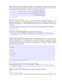
With the new user interface, PathWave allows to specify all necessary and optional parameters in an
optional configuration file, composed of “key=value” pairs as in the following example:
preprocessed.tag = KEGG.hsa
input.exprdata = my_expr_data_file.tsv
input.sampleclasses = my_class_file.tsv
param.kegg.only_metabolism = TRUE
param.ztransform = TRUE
param.numperm = 1000
param.pvalue.correction.method = Bonferroni
param.pvalue.threshold = 0.05
output.file.prefix = my_output_file_prefix
The expressions used as key (e.g. “input.exprdata”) are the argument names as defined for the
respective PathWave functions (see Sections 3 and 4 for their names and meaning).
The name of the configuration file can be passed to the respective PathWave functions. Otherwise
PathWave will try to load configuration parameters from the following default configuration files (in
the current working directory):
pathwave.preprocess.conf
pathwave.run.conf
[for preprocessing pathway data; see Section 3]
[for running PathWave; see Section 4]
Important notes:
• If an argument is both specified in the configuration file and passed to the respective PathWave
function, the value directly passed to the function takes precedence over the value specified
in the configuration file.
• Mandatory arguments must be specified either by directly passing them to the function call or
by specifying them in the configuration file.
3. Preprocessing pathways
[Note: if you just want to apply PathWave with already provided, preprocessed pathway data (see
Section 4.1 and Table 4.1), you can skip this section.]
PathWave maps the expression data to optimally arranged 2D grid representations of metabolic (and
signaling) pathway networks. The preprocessing of pathway information to produce the 2D grid
representations is only partly done with the PathWave R package itself, although the necessary external
source code is provided along with it (see Section 3.3).
3.1. Translating SBML files to KGML-like pathway files
PathWave requires pathway descriptions from XML files that respect the Kyoto Encyclopedia of Genes
and Genomes (KEGG) Markup Language (KGML), although not all features of KGML are used. For
users that instead wish to extract information on metabolic pathways from SBML files, we provide an
additional Perl script that translates an SBML file into a set of KGML(-like) XML files for use with
PathWave.
Important:
Please note that this has been tested only with the metabolic model of the Human recon 1 (Duarte et al.,
2007), taken from the BiGG database (Schellenberger et al. 2010) (see Section 4.1). Since the SBML
“standard” seems to be applied in a rather arbitrary fashion, there is no guarantee that the Perl script
will also work with other SBML files because it was developed for use with Recon1/BiGG.
To obtain the script, unpack the PathWave package file (.tar.gz or .zip) and take it from the subfolder
PathWave/src. Filename: rmp-extractReactionsFromBiGGreconsSBML.pl
Dependencies:
The script depends on the Perl module XML::TreeBuilder, freely available at www.cpan.org.
Run the script on your SBML file like in the following example. [Note, the description regards a
Unix/Linux system; the procedure may differ for Windows]
./rmp-extractReactionsFromBiGGreconsSBML.pl -f <your_sbml_file>
-E <file_with_metabolites_to_exclude>
-s -P <kgml_file_prefix> -O <sepcies_tag>
The most important command line arguments are:
• -f <file>
The input SBML file (mandatory).
• -E <file>
An additional file listing metabolites to be excluded (one per line); this allows to
ignore metabolites and chemical substances that do not provide meaningful information for inferring links between metabolic reactions (e.g. H2O). Metabolites
to be ignored are specified in terms of the corresponding species ID (reactant /
product) used in the SBML file; example: M_h2o_r.
• -s
The reactions gene associations will be simplified. The BiGG recon 1 SBML file
uses modified Entrez gene IDs that are followed by a dot and a digit to indicate
different isoforms (e.g. “1312.1” and “1312.2”). Since KEGG uses plain Entrez
gene IDs and expression data is mostly mapped to genes rather than their single
isoforms, this option allows to remove the information related to the isoform and
concentrate on plain Entrez gene IDs (e.g. “1312”).
• -P <prefix> If specified, the subsystems found in the SBML file will be interpreted as
pathways and written to a set of KGML(-like) XML files (one per subsystem)
named “<prefix><subsystem_name>.xml”. This is argument not mandatory for
using the script (that has also another purpose) but required for PathWave.
• -O <tag>
A KEGG-like species tag. Default: “hsa”.
Note: The script will write summary information of the found metabolic reactions to the standard
output. This information is not required for PathWave and can be ignored or redirected.
The KEGG(-like) pathway files written using option -P can be used for the preprocessing steps
described in the following Sections.
See the online help (on the shell command line) for further information:
./rmp-extractReactionsFromBiGGreconsSBML.pl -h
3.2. Producing adjacency matrices
The first step when preprocessing pathway information is to produce adjacency matrices from the
pathway descriptions. PathWave takes pathway descriptions from XML files that respect the Kyoto
Encyclopedia of Genes and Genomes (KEGG) Markup Language (KGML). KGML versions 0.7.0 and
0.7.1 have been tested.
Procedure:
1. Save the KGML files with filenames “<pathway_ID>.xml” in a directory. Each <pathway_ID>
is an identifier for a pathway, e.g. “hsa00280”; alternatively, pathway names may be used
instead of their IDs. No other files with the extension “.xml” should be in this directory.
2. Run the following PathWave function in R:
pathWave.preprocessPathways(preprocessed.tag="<my_ID_tag>",
input.file.pathwaydir = "<dir_with_KGML_files>",
input.file.pathwayid2name = "<file_mapping_pathway_ID_to_name>",
output.file.matrixdir = "<dir_where_to_store_adjacency_matrices>")
Alternatively, if parameters are specified in a configuration file, the function can be run with
pathWave.preprocessPathways(configfile="<my_conf_file>")
[The use of input.file.pathwayid2name is optional.]
Each produced adjacency matrix will be written with filename “<pathway_ID>.matrix” in the specified
matrix directory. Additionally, an R data file named “pwdata.pathways.<my_ID_tag>.rda” will be
written to the current working directory. This file contains the adjacency matrices and (optional)
mappings from pathway IDs to names that are used for running PathWave on expression data (see
Section 4).
Important notes:
• The chosen ID tag <my_ID_tag> should be unique. The use of tags associated with
preprocessed pathway data already provided with the package (see Table 4.1) should be
avoided.
• For pathways from KEGG, <my_ID_tag> should start with “KEGG”; this allows to later run
PathWave specifically on metabolic KEGG pathways, excluding signaling etc. (by running the
procedure with param.kegg.only_metabolism=TRUE ;see Section 4.2.1)
See the online help for further information:
?pathWave.preprocessPathways
3.3. Computing optimized 2D grid arrangements
This is the most critical step in the preprocessing of the pathway data. This step is not done using the R
functions provided with the PathWave package, but using additional C++ code (GridArranger)
provided along with the R package.
3.3.1. Required software
GridArranger has the following two important dependencies:
1) ABACUS v.2.4-alpha
To run the Grid Arranger, you will first need to install ABACUS v.2.4-alpha, developed by the
University of Cologne, Germany (Jünger and Thienel, 2000; Elf et al., 2001).
Important: Since GridArranger is NOT compatible with later versions of ABACUS (that can be
obtained from the ABACUS webiste at http://www.informatik.uni-koeln.de/abacus/), we provide the
required version (v.2.4-alpha) with kind permission of the original authors on the PathWave website at:
http://www.ichip.de/software/pathwave.html
Download the ABACUS package from the PathWave website and follow the instructions in the file
INSTALL in the main directory of the package. Choose "GCC 2.9" whenever ABACUS asks to specify
a compiler.
2) Linear program solver
ABACUS requires an external linear program solver. We recommend CPLEX, which is free for
academic research and available at http://www.ibm.com/software/integration/optimization/cplexoptimizer/. The following linear program solvers are also compatible: Cbc, Clp, DyLP, GLPK, Gurobi,
MOSEK, Soplex, SYMPHONY, Vol, XPRESS-MP.
3.3.2. Installation of GridArranger
GridArranger v1.0 is provided both within the PathWave 2.1. R package and as an independent
package at http://www.ichip.de/software/pathwave.html. To extract it from the R package, unpack the R
package and take the GridArranger package (file “GridArranger-v1.0.tgz”) from the subfolder
PathWave/src. Alternatively, download the GridArranger package from the PathWave website.
To install the Grid Arranger, unpack GridArranger-v1.0.tgz and open the file Makefile in its main
directory. Adjust the paths to ABACUS and CPLEX at the top of the file, then enter your preferred
GNU compiler. You should use the same compiler that you used to compile ABACUS. On a Unix/
Linux system, execute the following command from a shell:
make
3.3.3. Running Grid Arranger on pathway adjacency matrices
Copy the adjacency matrix files produced by pathWave.preprocessPathways() (see Section 3.2)
from output.file.matrixdir to the folder "in", which is located in the main directory of the
GridArranger. To start the computation on a Unix/Linux system, execute the following commands from
a shell:
cd <main directory of GridArranger>
chmod u+x runGridArranger
./runGridArranger
The Grid Arranger will arrange all files found in the input folder "in" and store the results in the output
folder "out". It will print status messages to your shell. After the calculation is finished, the file
"statistics.log" is being created in the output folder "out". It contains some information about the
success of the run as well as (possible) error messages.
In the unlikely case that for one of the input files no approximate solution could be found, e.g. if the
adjacency matrix is very large, you can try the following steps:
1) Rerun the solver. It contains several random elements, such that the results of different runs might
differ from each other.
2) Open the file ".abacus" in the folder "bin" and increase the parameter MaxCpuTime. By default, it is
set to 30 minutes for every input file.
After a successful arrangement of the adjacency matrix into compact 2D lattice grids, the Grid Arranger
output files can be used for the final preprocessing step that is again executed using the R package, as
described in the next Section.
3.4. Preparation of 2D grid arrangements for PathWave
The third and last step of preprocessing is the preparation of the externally computed 2D grid
arrangements (see Section 3.3) for the use with PathWave. This is done in R with the following
function call:
pathWave.preprocessOptGrids(preprocessed.tag="<my_ID_tag>",
input.file.pathwaydir = "<dir_with_KGML_files>",
input.file.optgriddir = "<dir_where_2D_grid_arrangements_are_stored>")
Alternatively, if parameters are specified in a configuration file, the function can be run with
pathWave.preprocessOptGrids(configfile="<my_conf_file>")
Result:
An R data file named “pwdata.optgrids.<my_ID_tag>.rda” will be written to the current working
directory. This file contains the optimally arranged 2D grid representations of the pathway networks
that are used for running PathWave on expression data (see Section 4).
Important notes:
• The identification tag “<my_ID_tag>” must be the same as used in Section 3.2.
• The pathway directory (input.file.pathwaydir) must be the same as used in Section 3.2.
• The directory of optimal grid arrangements ( input.file.optgriddir) is the directory where
the output files produced by Grid Arranger are stored (see Section 3.3).
See the online help for further information:
?pathWave.preprocessOptGrids
4. Running PathWave
This section explains how to run the PathWave algorithm with already preprocessed metabolic/
signaling pathways (that have been transformed in 2D grid representations; see Section 3) on gene
expression data for the purpose of identifying pathways whose regulation is significantly different
between two sample sets (e.g. normal and tumor tissue). In contrast to other methods, PathWave takes
the topology of metabolic networks into account (mapping them on optimally arranged 2D grids) and
can identify interesting pathways also if localized subnetworks show significant differences, e.g.
metabolic switches. For more details see Schramm et al. (2010) and Piro et al. (2014).
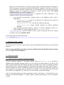
4.1. Preprocessed pathways provided with the package
Version 2.1 of PathWave comes with several preprocessed pathway data sets, such that for many
applications the steps described in Section 3 can be skipped. Table 4.1 lists all available pathway
datasets and their associated ID tags (preprocessed.tag) to be specified when running PathWave.
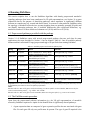
Table 4.1: Available preprocessed metabolic pathway data.
ID tag
Organism
Source
Gene IDs
BiGG.hsa
H. sapiens
Recon 1 (Duarte et al., 2007) / BiGG
database (Schellenberger et al. 2010)
Entrez gene IDs, e.g. “10000”
KEGG.hsa
H. sapiens
KEGG (Kanehisa et al., 2012);
downloaded April 14, 2011
Entrez gene IDs, e.g. “10000”
KEGG (Kanehisa et al., 2012);
downloaded April 14, 2011
Entrez gene IDs, e.g. “11674”
KEGG.mmu M. musculus
KEGG.dme
D. melanogaster KEGG (Kanehisa et al., 2012);
downloaded April 14, 2011
Gene symbols as used by KEGG, e.g.
“Dmel_CG11876” for CG11876 [Note #1]
KEGG.dre
D. rerio
KEGG (Kanehisa et al., 2012);
downloaded April 14, 2011
Entrez gene IDs, e.g. “321664”
KEGG.cel
C. elegans
KEGG (Kanehisa et al., 2012);
downloaded April 14, 2011
Locus tags, e.g. “LLC1.3” [Note #2]
KEGG.eco
E. coli
KEGG (Kanehisa et al., 2012);
MG1655 Gene IDs / ordered locus names,
downloaded April 14, 2011
e.g. “b2097”
Important: there is some inconsistency in the gene IDs used by KEGG, but we have opted for taking the IDs exactly as used
by the database from which we derive the pathway information.
Notes:
#1: This holds for >99% of all genes; mostly those having a CG ID as symbol. For the remainder, KEGG uses only the
symbol, without leading “Dmel_”, e.g. “COX1” and “CYTB”.
#2: This holds for >99% of all genes. For the remainder, KEGG uses the gene symbol, e.g. “COX1” and “CYTB”.
4.2. The PathWave main procedure
Apart from the preprocessed pathway information (e.g. the 2D grid representations of metabolic
networks), PathWave requires two inputs for the identification of significantly altered pathways:
i. A gene expression data set composed of gene expression profiles that are associated with gene
IDs. For each gene ID only one profile must be present. The type of gene ID required is the
same as used for the preprocessed pathway information (e.g. Entrez gene IDs for KEGG.hsa;
see Table 4.1).
ii. A mapping of the samples in the expression data set to two subgroups/classes that need to be
analyzed for differential expression of pathway components (e.g. normal and tumor; untreated
and treated; …)
The exact format of the required input data is described in detail in Section 4.2.1 (see also the “Usage
Example”/Quick Guide document for a practical example that illustrates the required input format).
To run PathWave, use the following R command:
pwres <- pathWave.run(preprocessed.tag="<ID_tag>",
input.exprdata=<my_expr_data>, input.sampleclasses=<my_sample_classes>,
param.kegg.only_metabolism=TRUE/FALSE,
param.ztransform=FALSE/TRUE, param.numperm=<num_permutations>,
param.pvalue.correction.method="Bonferroni/BH/...",
param.pvalue.threshold=<p_value_cutoff>,
param.filter.size=<num_genes_and_reactions>,
output.file.prefix="<my_out_prefix>", verbose=FALSE/TRUE)
Alternatively, if parameters are specified in a configuration file, the function can be run with
pwres <- pathWave.run(configfile="<my_conf_file>")
[Note: for the remainder of the manual we assume the function's return value to be stored in an object
named pwres! The same object name is used when saving results via output.file.prefix; see below.]
The function call returns a list object composed of three elements:
pwres$results.all: results for all pathways, whether significant or not
pwres$results.filtered: only filtered, significant pathways
pwres$results.table: human readable table with a summary of filtered, significant results
The following Sections describe mandatory and optional parameters in more detail.
4.2.1. Mandatory parameters to pathwave.run()
The following parameters MUST be specified either with the function call or in a configuration file:
•
preprocessed.tag="<ID_tag>": identifies which preprocessed pathway information has to
•
be used to map the expression data to metabolic networks. This can be either one of the
pathway data sets provided with the package (see Table 4.1) or a custom pathway data set
produced as described in Section 3. In the latter case, it is imperative to load the respective R
data files written by pathWave.preprocessPathways() and pathWave.preprocessOptGrids()
(“pwdata.pathways.<ID_tag>.rda” and “pwdata.optgrids.<ID_tag>.rda”; see Sections 3.2
and 3.4) before using them with pathWave.run()!
input.exprdata=<my_expr_data>: the gene expression data set on which to run PathWave.
This can be passed to pathWave.run() as
• a data.frame containing a matrix (row names must be Entrez gene IDs, column names
are sample IDs); or
• a file name from which to load the expression data. Required file format: Tab-separated
vector (TSV); the header line must contain only sample IDs and data lines must have an
additional preceding field containing the Entrez gene ID; hence data lines contain one
more field than the header line.
•
input.sampleclasses=<my_sample_classes>: definition of exactly two samples classes
for the expression data. This may be one of the following three:
• a factor matching exactly the columns in the expression data;
• a data.frame containing a table with two columns (1=sample ID, 2=class); or
• the name of a file containing a mapping from sample ID to class as TSV. File format: no
header; one mapping per line as “<sample_ID><tab><class>”.
Note: If the two classes/sample subsets are specified as a data.frame or as a file name, we have a
precise sample ID and can therefore also specify only a subset (in an arbitrary order) of the full
expression data (i.e. the full expression data set may contain further samples of other classes
that will not be used in the procedure). A factor, instead, does not contain sample IDs and must
therefore exactly match the number and order of samples contained in the expression data set.
Hint: PathWave will order sample class names alphanumerically and take the second as the
control. Example: for classes “normal” and “tumor”, the “tumor” class would be taken as a
control and hence “up-regulation” would mean that a reaction has a higher expression in
normal than in tumor. Therefore, in this case it may be wiser to name the classes something like
“1_tumor” and “2_normal” in order to make sure that “up-regulation” refers to a higher
expression in the tumor class. In any case, PathWave will report to which of the two classes the
notions “up-regulation” or “down-regulation” refer. In the above two examples, this would be
“normal” (instead of “tumor”) and “1_tumor” (instead of “2_normal”), respectively.
4.2.2. Optional parameters to pathwave.run()
The following parameters are optional, in most cases because default values will be used if they are
neither specified with the function call nor in a configuration file. Be sure you understand what the
default values mean before running PathWave.
•
•
•
•
•
•
param.kegg.only_metabolism=FALSE/TRUE: specifies whether only metabolic pathways
from KEGG should be evaluated. If TRUE (default), all other KEGG pathways (e.g. signaling,
DNA repair, etc.) will be ignored. However, the parameter is only used if PathWave is run with
preprocessed pathways from KEGG (recognized by having an <ID_tag> starting with “KEGG”;
see preprocessed.tag above).
param.ztransform=FALSE/TRUE: specifies whether expression data should be z-transformed
after it has been mapped to metabolic reactions (via the involved enzymes). The default is
TRUE for PathWave, but you may want to specify FALSE in case your expression data is
already z-transformed.
param.numperm=<num_permutations>: the number of randomizations/permutations to
perform for testing the statistical significance of the differential expression of metabolic
reactions or signaling genes. Default: 1000.
Note: The memory requirements but also the accuracy of P-values increase with the number of
permutations. (The default has been tested with a common PC with about 8 GB of RAM.)
param.pvalue.correction.method="Bonferroni/BH/...": the correction method for
multiple testing. For available methods, see the online help of p.adjust(): ?p.adjust
Default: “Bonferroni” for multiple testing correction according to the Bonferroni method.
param.pvalue.threshold=<p_value_cutoff>: the p-value cutoff for reporting interesting
pathways. Default: 0.05.
param.filter.size=<num_genes_and_reactions>: an additional filter that removes all
•
•
pathways for which less than <num_genes_and_reactions> metabolic reactions involving less
than <num_genes_and_reactions> genes are differentially expressed. This allows to filter out
cases in which, for example, a single enzyme is down-regulated but used several times in the
metabolic network of a pathway (i.e. involved in several network nodes). The default
minimum number of reactions and genes is: 3.
output.file.prefix="<my_out_prefix>": if specified the three components of the
returned list object will be saved in three files
• <my_out_prefix>-pw-results.rda: complete results in the PathWave object "pwres",
composed of
◦ pwres$results.all: results for all pathways (no filtering and correction for
multiple testing applied yet)
◦ pwres$results.filtered: only filtered, significant pathways
◦ pwres$results.table: human readable summary for filtered, significant
pathways
• <my_out_prefix>-pw-results_table.tsv: summary of filtered, significant results as a
human readable TSV table (corresponding to pwres$results.table).
verbose=FALSE/TRUE: specifies whether to print verbose information about the running
procedure to the screen. Default: TRUE.
See the online help for further information:
?pathWave.run
5. Analyzing the results
The following are a few hints on what results to expect from PathWave and how they can be mined and
analyzed.
Note: for most applications you will not need very detailed results and the hints given in Sections
5.1.1., 5.2. and 5.3. will be sufficient!
5.1. Returned results
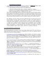
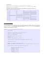
5.1.1. Human readable summary of significant pathways
The most important summary is the human readable table ( pwres$results.table) returned by
pathWave.run() (optionally written to the file “<my_out_prefix>-pw-results_table.tsv”; see above). The
table reports the significant (and filtered) pathways, the number of up- and down-regulated reactions
and the sample class to which the regulation is referred (the other sample class is the control). Table 5.1
shows an example, in which 18 metabolic reactions of the glycolysis / gluconeogenesis pathway are
down-regulated in the sample class “EC_affected” with respect to the other sample class, while only
one reaction is up-regulated in “EC_affected”; 14 reactions show no important changes.
Note: For signaling pathways the same terminology is used (“reactions.up”, “reactions.down”, etc.),
although the up-/down-regulation is actually regards signaling proteins/genes and not metabolic
rections.
Table 5.1: Example of a human readable output of PathWave
pathway.name
p.value
reactions.up reactions.nochange reactions.down regulation.direction
hsa00010 Glycolysis /
Gluconeogenesis
1.20e-05
1
14
18
EC_affected
hsa00561 Glycerolipid metabolism
2.96e-05
1
10
4
EC_affected
hsa00100 Steroid biosynthesis
3.09e-05
2
7
25
EC_affected
hsa00532 Glycosaminoglycan
biosynthesis - chondroitin
sulfate
4.36e-05
1
2
4
EC_affected
hsa00360 Phenylalanine metabolism
6.59e-05
1
6
3
EC_affected
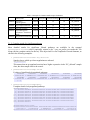
5.1.2. Complete results for significant pathways
More
detailed
results
for
significant,
filtered
pathways
are
available
in
the
returned
pwres$results.filtered object (optionally written to the “<my_out_prefix>-pw-results.rda” file
along with the complete results; see above). This object itself is a list composed of several elements, as
shown in the following examples:
•
pwres$results.filtered$r.reg.direction
Sample class to which up-/down-regulations are referred:
"EC_affected"
This means that an up-regulated reaction has a higher expression in the “EC_affected” sample
class; the other sample class is the control.
•
pwres$results.filtered$p.values
P-values of significantly dysregulated pathways:
hsa00010
hsa00561
hsa00100
hsa00532
hsa00360
hsa00830
1.206573e-05 2.960802e-05 3.094091e-05 4.363464e-05 6.593112e-05 9.436479e-05
hsa00980
hsa00480
hsa00670
hsa00052
hsa00562
hsa00590
1.116120e-04 3.462510e-04 4.069293e-04 5.453676e-04 6.151264e-04 7.099560e-04
[...]
•
pwres$results.filtered$pathway
Complete details for dysregulated pathways:
$hsa00010$reaction
[1] "hsa00010:R01662"
[5] "hsa00010:R01516"
[9] "hsa00010:R01070"
[13] "hsa00010:R02739"
[17] "hsa00010:R01786"
[21] "hsa00010:R00200"
[25] "hsa00010:R00703"
[29] "hsa00010:R00431"
[33] "hsa00010:R00711"
"hsa00010:R01512"
"hsa00010:R01061"
"hsa00010:R04780"
"hsa00010:R09086"
"hsa00010:R09085"
"hsa00010:R00746"
"hsa00010:R03270"
"hsa00010:R00726"
"hsa00010:R01788"
"hsa00010:R02740"
"hsa00010:R04779"
"hsa00010:R01600"
"hsa00010:R01602"
"hsa00010:R00754"
"hsa00010:R02569"
"hsa00010:R00235"
"hsa00010:R00959"
"hsa00010:R01015"
"hsa00010:R03321"
"hsa00010:R01518"
"hsa00010:R00658"
"hsa00010:R00014"
"hsa00010:R07618"
"hsa00010:R00710"
$hsa00010$reaction.p.value
hsa00010:R01662 hsa00010:R01512 hsa00010:R01788 hsa00010:R00959 hsa00010:R01516
7.533717e-01
4.012831e-04
2.982984e-05
1.001484e-05
7.533717e-01
hsa00010:R01061 hsa00010:R02740 hsa00010:R01015 hsa00010:R01070 hsa00010:R04780
1.999681e-05
hsa00010:R04779
3.167905e-06
hsa00010:R01518
1.516934e-01
hsa00010:R00200
3.504558e-06
hsa00010:R03270
4.973641e-01
hsa00010:R00235
4.201003e-01
3.409720e-06
hsa00010:R03321
3.409720e-06
hsa00010:R01786
1.539366e-01
hsa00010:R00746
2.584705e-05
hsa00010:R02569
5.436827e-01
hsa00010:R00710
3.726982e-01
4.486522e-06
hsa00010:R02739
3.409720e-06
hsa00010:R09085
3.657557e-02
hsa00010:R00754
1.611098e-03
hsa00010:R07618
1.650359e-01
hsa00010:R00711
5.172341e-01
3.890238e-07
hsa00010:R09086
3.657557e-02
hsa00010:R01602
9.868684e-01
hsa00010:R00014
4.973641e-01
hsa00010:R00431
2.740424e-03
1.311268e-01
hsa00010:R01600
1.539366e-01
hsa00010:R00658
1.755629e-04
hsa00010:R00703
1.875326e-02
hsa00010:R00726
2.740424e-03
$hsa00010$reaction.regulation
hsa00010:R01662 hsa00010:R01512
0
-1
hsa00010:R01061 hsa00010:R02740
-1
-1
hsa00010:R04779 hsa00010:R03321
-1
-1
hsa00010:R01518 hsa00010:R01786
0
0
hsa00010:R00200 hsa00010:R00746
-1
-1
hsa00010:R03270 hsa00010:R02569
0
0
hsa00010:R00235 hsa00010:R00710
0
0
hsa00010:R01788
1
hsa00010:R01015
-1
hsa00010:R02739
-1
hsa00010:R09085
-1
hsa00010:R00754
-1
hsa00010:R07618
0
hsa00010:R00711
0
hsa00010:R00959
-1
hsa00010:R01070
-1
hsa00010:R09086
-1
hsa00010:R01602
0
hsa00010:R00014
0
hsa00010:R00431
-1
hsa00010:R01516
0
hsa00010:R04780
0
hsa00010:R01600
0
hsa00010:R00658
-1
hsa00010:R00703
-1
hsa00010:R00726
-1
For each significant pathway, the reaction IDs ( pwres$reaction) are listed along with the
information (pwres$reaction.regulation) whether the reactions are up-regulated (1),
down-regulated (-1) or not differentially regulated (0), and along with the respective p-values
(pwres$reaction.p.value).
Results for single pathways can be accessed directly through, for example,
pwres$results.filtered$pathway$hsa00010; or more specifically thorugh
pwres$results.filtered$pathway$hsa00010$reaction,
pwres$results.filtered$pathway$hsa00010$reaction.regulation, and
pwres$results.filtered$pathway$hsa00010$reaction.p.value.
•
pwres$results.filtered$most.sign.pattern
Lists for each pathway the reactions/genes involved in the most significant pathway
feature(s)/pattern(s) [from Haar Wavelet transfroms] that gave rise to the pathway's p-value:
$hsa00010
[1] "hsa00010:R01662" "hsa00010:R01070" "hsa00010:R01788" "hsa00010:R04780"
[5] "hsa00010:R04779" "hsa00010:R01061" "hsa00010:R02740" "hsa00010:R01015"
$hsa00561
[...]
•
pwres$results.filtered$call
Lists the parameters used for multiple testing and filtering of the results
pw.result(x = "pw", pvalCutoff = 0.05, genes = NULL, filter = TRUE,
filter.size = 3, multtest = "Bonferroni", verbose = TRUE)
•
pwres$results.filtered$multtest
Method used for multple testing correction:
"Bonferroni"
•
pwres$results.filtered$pvalCutoff
P-value cutoff (after multiple testing) used for reporting significant results:
0.05
•
pwres$results.filtered$filter
Where the significant results filtered (see Section 4.2.1)? This is always true. To deactivate the
filtering, please set the filter size to zero.
TRUE
•
pwres$results.filtered$filter.size
Minium number of genes/reactions used for filtering (see Section 4.2.1):
3
•
pwres$results.filtered$version
Version of PathWave; specified as a date:
"2012-04-26"
•
pwres$results.filtered$url
Source location of the pathway information used:
"KEGG.hsa(2011-04-14)"
For own preprocessed pathway information, this corresponds to the pathway directory specified
as input.file.pathwaydir (see Section 3.2).
5.1.3. Complete results for all pathways
More detailed results for all pathways (whether significant or not) are available in the returned
pwres$results.all object (optionally written to the “<my_out_prefix>-pw-results.rda” file; see
above). This object itself is a list composed of the several elements, as shown in the following
examples:
•
pwres$results.all$r.reg.direction
Sample class to which up-/down-regulations are referred:
"EC_affected"
This means that an up-regulated reaction has a higher expression in the “EC_affected” sample
class; the other sample class is the control.
•
pwres$results.all$p.value
P-values (without multiple testing correction) for all pathways:
hsa05414
hsa04150
hsa04670
hsa04742
hsa00010
hsa04010
6.664114e-12 3.376588e-11 1.440104e-10 9.109923e-10 8.152520e-08 9.836255e-08
hsa00561
hsa00100
hsa00532
hsa00360
hsa04910
hsa00830
2.000542e-07 2.090602e-07 2.948287e-07 4.454805e-07 6.174754e-07 6.375999e-07
[...]
•
pwres$results.all$feat.p.value
P-values (without multiple testing correction) for all Wavelet-based features computed for the
pathways (see Schramm et al., 2010 for what is meant by “features”):
hsa00010:M1_row_LH_1_10 hsa00010:M1_org_LH_1_11 hsa01100:M54_org_HH_1_6
2.164481e-10
3.432276e-10
4.691022e-10
hsa01100:M54_org_HL_1_6 hsa01100:M54_org_LH_1_6 hsa01100:M54_org_LL_1_6
4.691022e-10
4.691022e-10
4.691022e-10
[...]
•
pwres$results.all$feat.reaction_list
Features that have been computed from the pathway network using the Haar Wavelet transform.
This vector maps the feature names internally used by PathWave to the lists of reaction/gene
nodes (separated by pipe symbols, “|”) that are involved in these features:
hsa00010:M1_org_LL_1_3
"hsa00010:R00431|hsa00010:R00658|hsa00010:R01518"
hsa00010:M1_org_LL_1_4
"hsa00010:R00014|hsa00010:R00200|hsa00010:R00726"
hsa00010:M1_org_LL_1_5
"hsa00010:R00703"
[...]
•
pwres$results.all$r.reg
Direction of regulation (up=1, down=-1) for all reactions and signaling proteins/genes of all
pathways with respect to the reference sample class (see above). Note: These results are not yet
filtered for significance, i.e. also reactions with high p-value are considered as either up or
down here.
hsa00010:R00014 hsa00010:R00200 hsa00010:R00235 hsa00010:R00431 hsa00010:R00658
-1
-1
1
-1
-1
[...]
•
pwres$results.all$r.p.value
P-values for a differential regulation of all reactions and pathways:
hsa00010:R00014 hsa00010:R00200 hsa00010:R00235 hsa00010:R00431 hsa00010:R00658
4.973641e-01
3.504558e-06
4.201003e-01
2.740424e-03
1.755629e-04
[...]
•
pwres$results.all$data
Summary information about the expression data on which PathWave was run. Note: this is after
mapping and grouping of expression profiles to metabolic reactions or signaling molecules,
hence the number of rows is the number of network nodes (metabolic reactions, signaling
molecules) to which the expression data has been mapped, not the number of genes for which
expression data was provided.
$x
$x$row
[1] 9095
$x$col
[1] 23
$x$overlap
[1] 3152
$y
[1] "EC_affected" "EC_control"
•
pwres$results.all$call
Lists the parameters used for processing the expression data
pw.pathWave(x = "x", y = "y", optimalM = "optimalGrid", nperm = 1000,
verbose = TRUE)
•
pwres$results.all$nperm
Number of randomizations/permutations performed for statistical evaluation:
1000
•
pwres$results.all$oM
This is a complex list object containing all necessary data for the preprocessed pathways. It is
composed of
pwres$results.all$oM$version, pwres$results.all$oM$url,
pwres$results.all$oM$pathways, pwres$results.all$oM$reactions, and
pwres$results.all$oM$data
The latter contains the adjacency matrices of the pathways in terms of reactions, e.g.
pwres$results.all$oM$data$hsa00010
$M1
[,1]
[,2]
[1,] "0"
"0"
[2,] "0"
"0"
[3,] "0"
"0"
[4,] "0"
"0"
[5,] "0"
"hsa00010:R01518"
[6,] "hsa00010:R00431" "hsa00010:R00658"
[7,] "hsa00010:R00726" "hsa00010:R00200"
[8,] "0"
"hsa00010:R00014"
[9,] "0"
"hsa00010:R00703"
[10,] "0"
"0"
[11,] "0"
"0"
[12,] "0"
"0"
[...]
[,3]
"hsa00010:R01015"
"hsa00010:R01070"
"hsa00010:R01061"
"hsa00010:R01662"
"hsa00010:R01512"
"hsa00010:R01516"
"0"
"hsa00010:R03270"
"hsa00010:R02569"
"hsa00010:R00235"
"hsa00010:R00710"
"0"
[,4]
"hsa00010:R04780"
"hsa00010:R04779"
"hsa00010:R02740"
"hsa00010:R01788"
"hsa00010:R00959"
"0"
"0"
"hsa00010:R07618"
"0"
"hsa00010:R00711"
"hsa00010:R00746"
"hsa00010:R00754"
5.2. Overall summary
An overall summary of the procedure can be obtained by passing the complete results for all pathways
(pwres$results.all) or the filtered, significant results ( pwres$results.filtered) to the function
pathWave.resultSummary(). Example:
pathWave.resultSummary(pwres$results.all)
pw.pathWave
Pathways: 202 pathways with 8260 reactions
Source url: KEGG.hsa(2011-04-14)
Version of 2012-04-26
Expression data: 9095 reactions
Samples: 23
Classes: EC_affected,EC_control
Overlap between expression and pathway reactions: 3152
Permutations: 1000
Number of features generated: 25470
Number of pathways with p.value <= 0.01: 100 and p.value <= 0.05: 100
Significance of regulation patterns (first 5):
pathway p.value(uncorrected)
hsa05414 6.7e-12
hsa04150 3.4e-11
hsa04670 1.4e-10
hsa04742 9.1e-10
hsa00010 8.2e-08
Note: if applied to the complete results (pwres$results.all), the reported p-values are NOT
corrected for multiple testing! For corrected p-values, see Sections 5.1.1 and 5.1.2.
See the online help for further information:
?pathWave.resultSummary
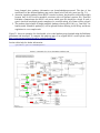
5.3. Obtaining colored pathway maps from KEGG
If the preprocessed pathway information has been derived from KEGG pathways (Kanehisa et al.,
2012), the differentially regulated pathways obtained from the PathWave analysis can be drawn as
metabolic networks with color-coded reactions/enzymes according to their regulatory status. This
service is provided externally by the KEGG website and not by PathWave itself. PathWave, however,
provides an easy to use function for building URLs that can be passed to any web browser for querying
the KEGG web server to retrieve custom pathway images with colored nodes (reactions or genes):
keggurls <- pathWave.getColorKEGGMapURLs(pwres$results.filtered,
preprocessed.tag="KEGG.hsa",
col=c("green","grey","red"),
col.sign.pattern=c("red","red","green"))
This function call returns a vector containing URLs with which the colored networks can be requested
from the KEGG web server. Example:
keggurls
[1] "http://www.kegg.jp/kegg-bin/show_pathway?hsa04140/64422%09red,green/10533
%09red,black/9140%09grey,black/11337%09grey,black/30849%09grey,black/5289
%09green,red"
[2] "http://www.kegg.jp/kegg-bin/show_pathway?map00471/rn:R00243%09green,red/
rn:R00248%09green,red/rn:R00256%09green,black/rn:R01579%09%23bfffbf,black"
[…]
As a default, nodes of up-regulated reactions/enzymes will be depicted in red, nodes of down-regulated
reactions in green, and the color gray will be used for other reactions that have been evaluated by
PathWave (i.e. whose involved genes had available expression data) but showed no significant changes.
Reactions/enzymes for which no data was available, will have the original color used by KEGG
pathway maps. The color code to be used for drawing PathWave results can be personalized using the
function argument “col”, as in the example above. Colors are specified as a string vector in the
following order: 1) color for down-regulation; 2) color for no changes; 3) color for up-regulation.
Default: col=c("green","grey","red")
Additionally, the font color of some nodes is changed to indicate which reactions/genes are involved in
the most significant pathway feature(s)/pattern(s) that gave rise to the pathway's p-value. Colors are
specified as a string vector in the following order: 1) font on down-regulated nodes; 2) font on nodes
without significant differences; 3) font on up-regulated nodes. Default: col.sign.pattern=
c("red","red","green")
Colors for both nodes and font can also be arbitrarily chosen and specified as hexadecimal RGB code
(e.g. “#FF0000” for red).
Important:
1. Keep in mind that the preprocessed pathway information used with PathWave may be older
than the pathway map currently available from the KEGG web server, hence the map may have
been changed since pathway information was downloaded/preprocessed. The date of last
modification of the obtained pathway map can be found in its lower left corner (see Fig. 5.1).
2. Attention: signaling pathways from KEGG can also be drawn, but should be verified thoroughly
because they do not involve metabolic reactions with well defined reaction IDs. Therefore
PathWave communicates the KEGG web server which gene IDs should be colored. If such a
gene is involved in multiple protein complexes (i.e. network nodes), all of them will be colored!
3. The pathway that includes all single metabolic pathways (having ID 01100, e.g. “hsa01100” for
human; name “Metabolic pathways”) will be ignored because drawing it with all up- and downregulations is a too complex task.
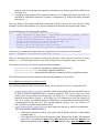
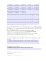
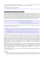
Figure 5.1 shows an example of a downloaded, color-coded pathway map obtained using the PathWave
procedures and interfaces. To compare this pathway map to its original KEGG version please check
http://www.genome.jp/kegg-bin/show_pathway?hsa00670.
See the online help for further information:
?pathWave.getColorKEGGMapURLs
Figure 5.1: Example of a color-coded KEGG pathway map.
Acknowledgements:
We thank Zita Soons (Maastricht University) and Ashwini Kumar Sharma (DKFZ) for proof-reading
and testing, and the DKFZ Data Management team for the continuous support.
References:
•
•
•
•
•
•
•
Duarte et al. (2007) Global reconstruction of the human metabolic network based on genomic
and bibliomic data. Proc. Nat. Acad. Sci. USA 104(6):1777-1782.
Elf et al. (2001) Branch-and-Cut Algorithms for Combinatorial Optimization and Their
Implementation in ABACUS. Lecture Notes in Computer Science 2241:157-222.
Jünger, Thienel (2000) The ABACUS system for branch-and-cut-and-price algorithms in
integer programming and combinatorial optimization. Software: Practice and Experience
30:1325-1352.
Kanehisa et al. (2012) KEGG for integration and interpretation of large-scale molecular data
sets. Nucleic Acids Res. 40:D109-D114.
Piro et al. (2014) Network topology-based detection of differential gene regulation and
regulatory switches in cell metabolism and signaling. submitted.
Schellenberger et al. (2010) BiGG: a Biochemical Genetic and Genomic knowledgebase of
large scale metabolic reconstructions. BMC Bioinformatics 11:213.
Schramm et al. (2010) PathWave: discovering patterns of differentially regulated enzymes in
metabolic pathways. Bioinformatics 26(9):1225-1231.