Download Brain Vision Analyzer User Manual Version 1.05

Brain Vision Analyzer
User Manual
Version 1.05
© Brain Products GmbH 1999 - 2006
The Brain Vision Analyzer software, frequently abbreviated to Analyzer, is designed
exclusively for use in medical research. Brain Products GmbH does not grant warranty or
assume liability for the results of using the Analyzer.
The content of this document is the intellectual property of Brain Products GmbH, and is
subject to change without specific notification. Brain Products GmbH does not grant warranty
or assume liability for the correctness of individual statements herein. Nor does Brain
Products GmbH enter into any obligation with regard to this document.
Any trademarks mentioned in this document are the protected property of their rightful
owners.
4th August 2006
2
Contents
1.
Product declaration ..........................................................................................6
1.1. Product identification .......................................................................................6
1.2. Area of application ...........................................................................................6
2.
Introduction.......................................................................................................7
3.
Installation.........................................................................................................8
4.
Getting started and handling the program .....................................................9
5.
Segmentation ..................................................................................................15
6.
Montages.........................................................................................................16
7.
Views ...............................................................................................................21
7.1. Overview........................................................................................................21
7.2. Standard view ................................................................................................25
7.3. Grid view........................................................................................................26
7.4. Head view......................................................................................................30
7.5. Mapping view.................................................................................................32
7.6. 3D mapping view ...........................................................................................35
7.7. Special properties of frequency views (standard, grid and head) ..................36
7.8. Block markers and transient transforms ........................................................38
7.9. Overlaying different data sets ........................................................................40
7.10. Setting markers manually ..............................................................................42
8.
Automation through history templates.........................................................43
9.
Macros .............................................................................................................46
10.
Transforms......................................................................................................48
10.1. Primary transforms ........................................................................................49
10.1.1. Artifact Rejection......................................................................................49
10.1.2. Average ...................................................................................................55
10.1.3. Averaged Cross Correlation ....................................................................58
10.1.4. Band-rejection filters ................................................................................60
10.1.5. Baseline Correction .................................................................................62
Vision Analyzer User Manual
3
10.1.6. Change Sampling Rate............................................................................63
10.1.7. Coherence ...............................................................................................64
10.1.8. Covariance ..............................................................................................67
10.1.9. Comparison .............................................................................................69
10.1.10.
Current Source Density (CSD)...........................................................73
10.1.11.
DC-Detrend........................................................................................75
10.1.12.
Edit Channels ....................................................................................77
10.1.13.
Fast Fourier Transform (FFT) ............................................................79
10.1.14.
Filters .................................................................................................84
10.1.15.
Formula Evaluator .............................................................................86
10.1.16.
Frequency extraction .........................................................................88
10.1.17.
ICA (Independent Component Analysis)............................................89
10.1.18.
Level Trigger......................................................................................92
10.1.19.
Linear Derivation................................................................................94
10.1.20.
Lateralized readiness potential (LRP)................................................96
10.1.21.
MRI Artifact Correction ......................................................................99
10.1.22.
New Reference ................................................................................115
10.1.23.
Ocular Correction.............................................................................117
10.1.24.
Peak Detection ................................................................................121
10.1.25.
Pooling.............................................................................................125
10.1.26.
Raw Data Inspector .........................................................................126
10.1.27.
Rectify..............................................................................................132
10.1.28.
RMS (Global Field Power) ...............................................................133
10.1.29.
Segmentation...................................................................................134
10.1.30.
The t-test..........................................................................................142
10.1.31.
Wavelets ..........................................................................................145
10.1.32.
Wavelets / Layer Extraction .............................................................157
10.2. Secondary transforms..................................................................................158
10.2.1. Grand Average ......................................................................................158
10.2.2. Principal Component Analysis (PCA) ....................................................160
10.3. Transient transforms....................................................................................165
10.3.1. 3D Map ..................................................................................................165
10.3.2. Current Source Density (CSD)...............................................................166
4
10.3.3. Fast Fourier Transform (FFT) ................................................................167
10.3.4. Map........................................................................................................168
10.3.5. Zoom .....................................................................................................169
11.
Export components ......................................................................................170
11.1. Simple export components ..........................................................................171
11.1.1. Besa ......................................................................................................171
11.1.2. Generic Data Export ..............................................................................172
11.1.3. Markers Export ......................................................................................175
11.2. Extended export components ......................................................................176
11.2.1. Area Information Export.........................................................................176
11.2.2. Peak Information Export ........................................................................178
12.
Importing data, positions and markers.......................................................180
12.1. Importing data..............................................................................................180
12.1.1. Besa format ...........................................................................................180
12.1.2. Generic Data Reader.............................................................................181
12.2. Importing markers and channel positions ....................................................188
13.
Printing ..........................................................................................................189
14.
Exporting graphics .......................................................................................192
15.
Appending multiple raw data sets...............................................................193
16.
Solutions .......................................................................................................194
Annex A: Raw data on removable media.............................................................196
Annex B: Electrode coordinate system ...............................................................197
Annex C: Markers (time markers) ........................................................................198
Annex D: Keyboard shortcuts ..............................................................................200
Annex E: Installation Network License (USB).....................................................201
Annex F: Individual user profiles .........................................................................202
Annex G: Command-line parameters ..................................................................203
Annex H: Links to raw data...................................................................................204
Vision Analyzer User Manual
5
1. Product declaration
1.1.
Product identification
Product name:
Brain Vision Analyzer
Vendor:
Brain Products GmbH
Stockdorfer Straße 54
D-81475 Munich
Classification in accordance with
German legislation covering medical products:
UMDNS number:
Class I
Analysis software for EEG and evoked
potentials (16-307)
This product conforms to the Medical Device Directive (MDD) 93/42/EEC.
1.2.
Area of application
The Brain Vision Analyzer is used to analyze EEG signals using a personal computer.
The program may only be used by doctors or suitably trained personnel for research purposes
only.
6
2. Introduction
The Vision Analyzer evaluates raw EEG data both for spontaneous EEG analyses and for
evoked potentials.
Among other things, the program's features include:
•
EEGs with an infinite number of channels can be processed.
•
The maximum EEG length that can be processed exceeds 2 billion data points, regardless
of the number of channels.
•
EEG formats from various major makers are recognized. The number of readable formats
is constantly growing.
•
History trees record every single operation on EEG data.
•
Templates can be created from history trees which, in turn, can produce new history trees
automatically.
•
The Vision Analyzer can be controlled remotely by other programs as OLE Automation
has been implemented in it.
•
A built-in Basic interpreter allows users to create both simple command files for analysis
automation and sophisticated applications.
•
The individual parts of the program have a modular structure. There are reader, transform,
montage, export and view components. The program's functionality can be extended by
adding new components. Brain Products is constantly working on new components. All
interfaces are disclosed so skilled users can develop their own components, or have them
made to order.
Vision Analyzer User Manual
7
3. Installation
It is essential to install the program with setup.exe because the files on the disk are
compressed and have to be unpacked in a specific way.
System requirements
•
•
•
Windows 98, Windows NT 4.0, Windows 2000 or Windows XP
Minimum configuration: Intel 400 MHz Pentium II or compatible processor, 64 MB
RAM, graphics card with a resolution of 1024 x 768 pixels and 32,768 colors
The monitor used should have a screen size of at least 21 inches (53 cm) measured
diagonally.
100 MB of available disk space; further space requirements depend on the size of the data
that is processed
Installation
•
•
Start Windows 98, NT, 2000 or XP.
Insert the program CD-ROM in your CD-ROM drive.
If your computer supports autostart of CD-ROMs a menu will appear after a short time to
guide you through the installation process. Otherwise do the following:
•
•
•
•
Choose Start > Run from the task bar.
Click the Browse button.
Access your CD-ROM drive, choose setup.exe on the CD-ROM and click the Open
button.
Now follow the instructions that the program outputs.
Before launching the Analyzer insert the hardlock key (dongle) that comes with the package
in one of the printer ports on your computer. You can still operate a printer on this port simply
by connecting it to the hardlock key. It is also possible to connect several dongles to a port by
inserting one into another.
If you have acquired a network license, see the Annex "Installing a network license" for
installation details of the Hardlock Network Dongle.
Now launch the Analyzer by double-clicking the Vision Analyzer icon on the desktop.
An alternate way of launching the Analyzer is from the task bar: Start > Vision Analyzer.
8
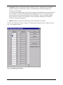
4. Getting started and handling the program
Launch the Analyzer.
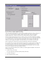
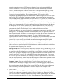
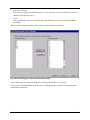
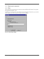
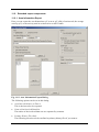
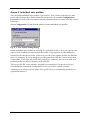
A window that is split into two panes appears on the left – the History Explorer. The first
thing you have to do is set up a workspace to tell the History Explorer where your data and
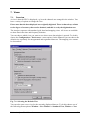
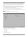
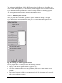
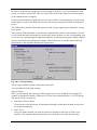
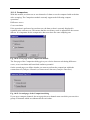
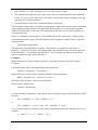
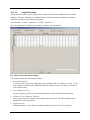
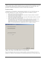
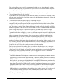
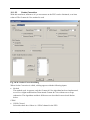
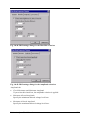
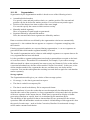
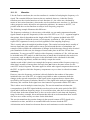
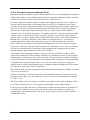
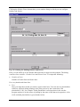
new history files are located. Choose File > New Workspace... to do this.
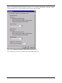
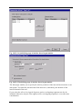
Fig. 4-1: New Workspace dialog
The program asks you for the folders containing the raw data files, history files and any
export files that you may want to use to export the results of your analyses.
Raw data files are EEG files that you have acquired. Specify the folder in which they are
stored. You can also look for the required folder by clicking the Browse button.
History files hold all processing steps (transforms) that you apply to the raw data. It is history
files that are shown graphically in the History Explorer later. Define any folder for the history
files.
Export files contain data that is intended to be processed further in other programs.
Once you have defined the settings, press the Enter key or click the OK button.
Now a dialog appears asking you to specify the workspace file. Give the file a meaningful
name and press the Enter key or click the Save button.
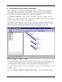
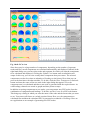
The raw data is now analyzed. A history file is created for every raw data file. A book icon
appears in the upper pane of the History Explorer for every history file. If nothing appears,
either the specified raw file folder is empty or the Analyzer cannot (yet) read the format of the
EEGs that are there. In the latter case, please get in touch with us to find out about the EEG
readers that are currently available.
When you have successfully read in one or more EEG files you can open a history file.
To do that, click the (+) sign on the left of the book icon. The entry expands and a Raw Data
icon appears. Double-click this icon. The EEG is displayed.
Vision Analyzer User Manual
9
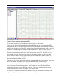
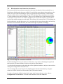
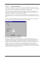
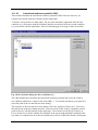
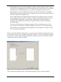
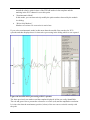
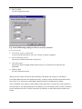
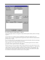
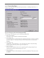
Fig. 4-2: Vision Analyzer with a loaded EEG
To navigate through the EEG, use the navigation bar that is at the bottom.
On the left, the navigation bar has four buttons with which you can move through the EEG
along the time axis. To the right of these buttons there is the marker window which shows all
markers that have been set in this EEG. Markers are all time-related indicators such as stimuli,
responses, comments, segment boundaries, DC corrections etc. There is a slider window
beneath the marker window. The width of a blue slider in this window represents the currently
displayed section, whereas the window itself represents the entire EEG. The slider can be
moved with the mouse. If you move the mouse to the marker window and press the right
mouse button, a context menu is displayed and you can hide the entire marker window or
choose specific marker types. Clicking any position in the marker or slider window displays
the corresponding section of the EEG.
You can use the tool bar, which is located at the top beneath the menu, to define the time span
shown, the number of channels to be displayed simultaneously, and other aspects.
You can obtain help on the functions of the navigation and tool bars by positioning the mouse
on the buttons or various elements on them. After a short time a tooltip with some brief
information will appear in a small yellow window. At the same time, the status bar at the
bottom of the program window will display some more details.
In addition, the status bar contains seven windows which give information on montage, the
segment displayed, mouse position and the current workspace.
10
The first window shows the current montage in magenta font. Montages are dealt with in
detail later.
The second window indicates the time that corresponds to the beginning of the displayed EEG
interval in blue font. The third window shows the current segment number at the beginning of
the displayed EEG interval – also in blue font. Segments are also described in more detail
later.
The next three windows show the mouse position in red font. The first window in this group
contains the name of the channel that the mouse is over. The second window indicates the
applied voltage there, and the third window states the time relative to the beginning of the
displayed EEG section or relative to any Time 0 marker that has been set (also explained
later).
The final window shows the name of the active workspace in black font.
To carry out a simple operation at this juncture just choose Transformations > Filters....
This brings up a dialog box in which you can define various filter settings. The different
transforms are explained later. Simply press OK at this point. All transforms can be undone
later without any problems. Note that the Analyzer never changes original EEGs. After a
short while another window opens and displays the new data set that has been generated as a
result of this operation. It is also shown in the History Explorer as a new icon named Filters.
Choose Transformations > RMS (Global Field Power...) now. A dialog consisting of two
windows appears, showing available channels on the left and selected channels on the right. If
no channel names are displayed in the right-hand window, double-click some channels in the
left-hand window to make them appear on the right. Pressing OK opens a new window
displaying the results of the operation. Something has happened in the History Explorer, too.
An RMS icon has attached itself to the Filters icon. Further operations make the history file
grow more.
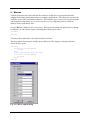
There can also be multiple branches from a data set. Let's assume you want to perform other
analyses on your raw data which do not require a filter. In this case you select the raw data as
the current window by clicking on the open raw data window. Alternately you can doubleclick the Raw Data icon in the History Explorer. Now choose Transformations > RMS
(Global Field Power...) again, for example. Choose a few channels again and press OK. A
new RMS icon appears beneath Filters. The history list has branched, giving rise to a history
tree. Analyses can be created as branches at any point in this way.
Vision Analyzer User Manual
11
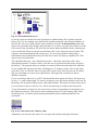
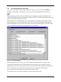
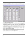
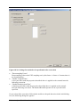
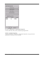
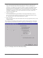
Fig. 4-3: Branched history tree
If you now want to transfer the same operations to another history file, open the required
history file. For our example, note that this file should contain the same channel numbers as
the first file. Now you could call the same transforms from the Transformations menu and
answer the questions in the dialogs again, but there is an easier way. Move the mouse over the
Filter icon for the first history file, press the left mouse button and hold it down, and drag the
icon over the Raw Data icon for the second history file. Now release the mouse button. The
Analyzer will automatically build a history tree. It is not only possible to drag history
information between different history files but also to store it in history template files. This
aspect is also described later.
The individual data sets – also called history nodes – that make up a history file can be
deleted and renamed. To delete a node, select the one in question with the mouse and press
the Del key. The program asks you whether you want to delete the node and all its subnodes.
If you confirm this question, the node will disappear. To rename a node, select it and either
press the F2 key or click the node text again after a short while. The text can now be edited
and you can change it to meet your requirements. This approach is identical to that in
Windows Explorer.
If you create larger data sets (e.g. FFT) and then delete them again, the history file may keep
its size, i.e. it may contain gaps. To remove such gaps, move the mouse pointer to the icon for
the history file in question and press the right mouse button. This opens a context menu where
you can choose Compress History File. It does not take long to compress the history file.
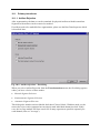
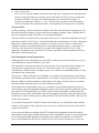
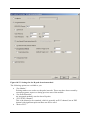
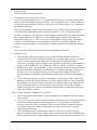
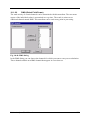
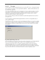
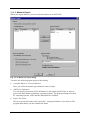
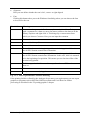
To get information on a data set, move the mouse to the corresponding icon and again press
the right mouse button. This opens a menu containing Operation Infos among other items.
Select this item. A window opens showing information on the transform that has been
performed.
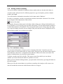
Fig. 4-4: Context menu for a history node
Alternately you can move the mouse over an open data window and right-click there.
12
You close a history file by clicking the (-) sign next to the book icon. This automatically
closes all data set windows associated with the file.
Now is the time to introduce two new terms: primary and secondary history files. You have
already encountered primary history files. They populate the upper pane of the History
Explorer. What characterizes primary history files is that they represent a specific raw EEG
and its processing steps. Secondary history files generally represent operations which are
applied to various nodes in various primary history files. An example of this is Grand
Average.
These secondary history files do not relate to a specific raw data EEG. They are stored in the
lower pane of the History Explorer. You can delete and rename secondary history files in the
way described above for history nodes. You cannot delete or rename primary history files in
the Analyzer.
You can use the mouse to shift the divider bar between primary and secondary history files up
or down.
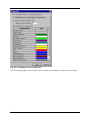
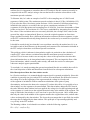
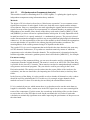
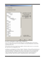
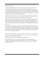
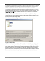
You can also assign colors to the individual transforms. These will appear in the
corresponding History Explorer icon and in the frame of views. You access the color
definition menu under Configuration > Preferences..., on the Transformation Colors tab.
You will find the following options there:
•
Use Different Colors to Indicate Different Transformations
Here you define whether you want to give different colors to different transforms.
•
Add a Color Frame Around the Views
If you enable this option, views appear in a frame which has the defined color. The Width
of Color Frame subitem defines the width of the frame in pixels.
•
Press Color Button to Change a Color
You can assign the actual colors in this table.
Vision Analyzer User Manual
13
Fig. 4-5: Assigning colors to transforms
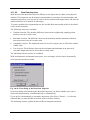
The following chapters deal with the various options offered by the Analyzer in more detail.
14
5. Segmentation
At this juncture we want to outline what segmentation is because the following chapters refer
to it repeatedly.
Segmentation means the division of an EEG into sections. Segmentation can be based on
different criteria. We use segmentation in the following cases:
•
As a preliminary stage in the analysis of evoked potentials. In this process, epochs of the
same length are generated relative to a reference marker (e.g. a stimulus). This results in a
data set of appended segments or epochs. Owing to the extensive facilities provided by
segmentation in the Analyzer, it is also possible to calculate averages according to
complex stimulus conditions (e.g. behavior-dependent conditions).
•
In preparation for separate processing steps in different sections of an EEG, for example
to analyze different stages before and after medication. In this case, sections are chosen
either manually or on the basis of a fixed time schedule and are converted into new data
sets in the history file which can then be analyzed separately.
No matter whether a data set is viewed before or after segmentation you can input your
preferences regarding the initial settings of montages and views when new data windows are
opened. Montages and views are explained in the following chapters.
You will find more information on segmentation in the "Segmentation" section of the
"Transforms" chapter.
Vision Analyzer User Manual
15
6. Montages
Montages enable channels to be reconnected on a software basis, i.e. new voltage references
are assigned to the channels.
They also serve to optimize the display of data, e.g. by combining frontal electrodes in one
montage and occipital electrodes in another one. In this case, when a montage is selected,
only those channels which have been assigned to it are displayed. The sequence of channels
can also be changed in a montage so that channels which were originally apart can be shown
next to each other. A channel can also occur multiple times in a montage.
Another important characteristic of a montage in the Analyzer is that certain display
parameters, such as position and size of a channel, can be assigned to it in a head view. A
head view is a view in which the channels can be positioned freely in the window. Its size can
be changed to meet particular requirements. The head view option is explained in more detail
in the next chapter.
A montage is used for visualization purposes only, i.e. the new data exists just temporarily
and the original data is not changed in any way.
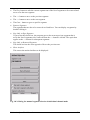
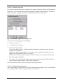
Fig. 6-1: New Montage start dialog
Choose Display Montage -> New.... from the menu in order to create a new montage. This
brings up a dialog in which you are asked about the type of reference to be used in the new
montage. There are four options:
•
Original. No new reference is calculated here. This type of montage is only used to group
channels or optimize their presentation as described above.
•
Average. The average reference is calculated here, i.e. the average of all selected channels
is used as the reference.
16
•
Laplacian. Source derivation according to Hjorth. This is a method derived from the
Laplace transform in which the reference is calculated from multiple neighboring
electrodes of a channel.
To ascertain the neighboring electrodes, the program needs information on the position of
the electrodes. If you used electrode names according to the 10/10 or 10/20 system for
data acquisition, the program should have this information. If you used other channel
names, however, then you can input the correct coordinates with the aid of the Edit
Channels transform component.
•
Bipolar. Bipolar connection. Differences between channels are formed.
Choose one of the four reference options. To begin with, it may be better to take the easiest
one – the original reference.
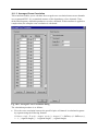
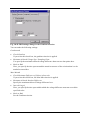
Fig. 6-2: Montage edit menu
Vision Analyzer User Manual
17
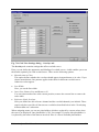
Clicking the OK button takes you to the edit menu for electrodes. You will see two columns
titled Chn (+) and Chn (-) which indicate the channels and their reference channels. The
second column is not accessible if you chose bipolar reference. On the right, the obligatory
OK and Cancel buttons are followed by others:
•
Insert Line: This button becomes accessible when you have written a text in the first field
of the first channel. If you click this button, the program inserts a line above the current
line.
•
Remove Line: With this button you can remove the current line providing it is not the last
line.
•
Insert Current Channels: This button is accessible providing you did not choose bipolar
montage, a data window has been activated and the montage list is empty. Clicking it
causes all channels in the current data window to be copied to the montage in their
original sequence. Then you may be able to define the required montage faster by
removing and inserting individual channels.
•
Remove All: This button becomes accessible when an entry has been completed. If you
click it, the entire content of the montage is removed following a question checking that
you really want to do so.
•
Arrange for Grid Views...: This button opens another dialog box in which the channels
for grid views can be arranged. The "Grid view" section of the "Views" chapter gives
more information on this.
If you opted for source derivation, another input box appears at the bottom of the dialog in
which you can specify the number of neighboring electrodes to be included in reference
calculation.
You can either type in the channel names or select them from the list boxes. If a data window
has been activated, its channels are available for selection. Otherwise channels according to
the 10/10 system are at your disposal. However, you can also type in any names which are not
listed in the boxes. When you have completed the first 16 channels, you can access the next
channels with the scroll bar.
As far as non-bipolar montages are concerned, the program inserts adequate names in the
reference channel input boxes.
When you have defined your montage, click the OK button. You are prompted to save the
montage. Input a suitable name and save the file.
To test your new montage, first make sure that a data window is active. Then click the
Display Montage menu. The number of items on the menu has increased as the name of your
new montage appears here now. Choose your new montage. The EEG is now displayed with
the montage. To revert to the default montage, choose it on the Display Montage menu.
If you want to modify an existing montage, select it under Display Montage > Edit... and edit
it. However, you cannot change the reference type for an existing montage. After editing the
program asks you again which name you want to store the montage under. You can input a
new name in order to derive a new montage from an existing one in this way.
18
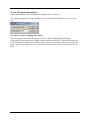
You can assign keyboard shortcuts to montages so that you can switch between them faster.
The montages are activated when you press the specified shortcuts. You can define these
shortcuts under Display Montage > Options.... The montages are assigned to the Ctrl-1 to
Ctrl-0 key combinations. Ctrl-1 is reserved for the default montage. As far as the other
combinations are concerned, you can select from existing montages.
Fig. 6-3: Keyboard shortcuts for montage selection
Vision Analyzer User Manual
19
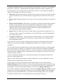
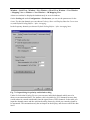
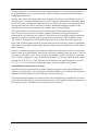
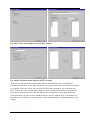
You can also choose a montage which is activated when a new data window is opened. To do
this, choose the Configuration > Preferences... option from the menu, and then the Views
tab. Here you can choose the default montage separately for unsegmented and segmented data
sets.
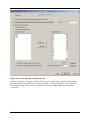
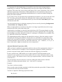
Fig. 6-4: Selecting the Default Montage
20
7. Views
7.1.
Overview
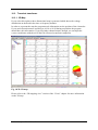
A view is how the EEG is displayed, e.g. how the channels are arranged in the window. You
have a variety of options to change the view.
Please note that the data displayed was originally digitized. There is thus always a limit
to the degree of accuracy that can be obtained, and this is set by the digitization rate.
The Analyzer operates with standard, grid, head and mapping views. All views are available
to show data in the time and frequency domains.
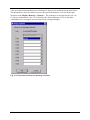
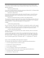
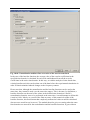
You can choose which view you want to use when a new data window is opened. To do this,
choose the Configuration > Preferences... menu option. On the View tab you can choose the
default view separately for unsegmented and segmented data sets. The mapping view cannot
be chosen here.
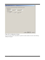
Fig. 7-1: Selecting the Default View
You can also open a new view for the currently displayed data set. To do this choose one of
the following menu options: Window > New Window > Standard View, Window > New
Vision Analyzer User Manual
21
Window > Grid View , Window > New Window > Head View, Window > New Window
> Mapping View or Window > New Window > 3D Mapping View.
A data set can thus be displayed simultaneously in several windows.
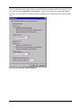
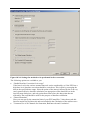
On the Scaling tab under Configuration > Preferences you can set the parameters for the
views. For the time domain you can choose Polarity, Start with Display Baseline Correction
on, and Default Scaling Before / After Averaging.
In the frequency domain you choose Default Scaling Before / After Averaging here.
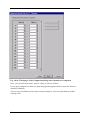
Fig. 7-2: Input dialog for polarity and default scaling
Under Set Individual Scaling Factors you can enter individual channels which are to be
shown on an attenuated basis. For instance, this is desirable for ECG channels because they
would otherwise extend considerably into the signal form of EEG channels. In the table you
input the channel names and the associated scaling factors by which you want the signals to
be attenuated. This attenuation only has an impact on the display, and does not affect the data
itself.
22
When you open a view, you can manipulate the output of the EEG with some elements from
the tool bar.
Fig. 7-3: Tool bar
Here are the elements that are relevant to views:
Overlay different data sets.
Increase the time shown.
Reduce the time shown.
Set a time shown that can be selected individually.
Reset the interval shown to the default value (Configuration > Preferences).
Show full segment. This button causes precisely one segment to be shown. It is only
accessible when the segments are small enough.
Increase scaling (sensitivity).
Reduce scaling (sensitivity).
Reduce the number of channels shown.
Increase the number of channels shown.
Go to next group of channels. This button is only accessible when a reduced number of
channels is being shown.
Go to previous group of channels. This button is only accessible when a reduced number
of channels is being shown.
Turn baseline correction on/off. Only the baseline of the display is changed, not the data
itself.
Set scaling.
Reset scaling to original value.
Set options for different views. These options are described in the following sections.
Turn marker edit mode on/off. This mode is described in the "Setting markers manually"
chapter.
Turn History Explorer on/off.
Cascade all view windows.
Vision Analyzer User Manual
23
Tile view windows side by side.
Tile view windows one after another.
The navigation bar is used to move along the time axis.
Slider
Marker window
Fig. 7-4: Navigation bar
The buttons on the left (1s) support forward/backward navigation by one second or, if a
section is ≤ 1 second, by 100 ms.
The buttons that follow are used to switch forward/backward by the displayed interval minus
one second, i.e. the intervals shown in succession overlay each other by one second.
To the right of these buttons you will see the marker window and beneath that the slider
window. Both of these windows represent the entire EEG in their width. The blue slider
represents the section that is currently being shown.
You can grab the slider with the left mouse button and drag it to the left or right. The EEG
display is updated accordingly when you release the mouse button.
You can also left-click both in the marker window and in the slider window. In this case, the
EEG display is positioned accordingly.
Pressing the right mouse button in the marker window opens a context menu on which you
can choose the marker types that you want to display.
The following sections describe the special properties of standard, grid, head and mapping
views.
24
7.2.
Standard view
The standard view corresponds to the EEG on paper. The curves are shown one under
another. The standard view is the one used normally for spontaneous EEG analyses.
You can display a channel on its own by double-clicking its channel name. Another doubleclick on the channel name takes you back to the original view.
If you want to show a selection of channels, mark all the ones you want in the required order
with a single mouse click. Double-clicking the last channel name selected then outputs the
selection. Another double-click on one of the channel names takes you back to the original
view.
During the selection process you can deselect a channel by clicking it again. Bear in mind that
a little time must pass before you can click the name again (approx. 0.5 – 1 second) because
the system would otherwise interpret the two clicks as a double-click.
Press the following button on the tool bar to turn the scaling bars on the left-hand side on or
off:
Set Display Features
A dialog appears in which you can turn the scaling bars on or off.
Vision Analyzer User Manual
25
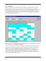
7.3.
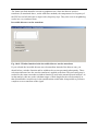
Grid view
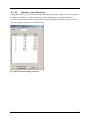
In this view, the channels are arranged in a grid. There is a standard grid for the default
montage. As far as other montages are concerned, you can define a grid yourself in the
montage edit dialog under Arrange for Grid Views... (also see the "Montages" chapter). Here,
you can input the required number of rows and columns in the channel grid. Pressing the
Refresh button updates the grid that is on the screen. Now you can arrange the channels and
the gaps between using the mouse.
Fig. 7-5: Grid definition dialog
In order to follow the descriptions below you should display an EEG and then activate a grid
view via Window > New Window > Grid View.
If you want to overlay two or more channels, move one channel over another one so that the
upper left corners of the two channels coincide. The border color of the motion indicator
changes to red. Drop the channel by releasing the left mouse button. You will see two
overlaid channels. The original channel that you moved is still at its original position. You
can repeat this operation with different channels as often as you need to. As soon as an
overlay exists, a button labeled Clear Overlays appears at the top right of the data window.
The overlays disappear when you click it.
26
To zoom into a channel, with or without overlaid channels, double-click the channel name.
The channel then occupies the entire data window. Now you can also apply the Delta Tool. If
you activate this by pressing the Delta Tool button, you can measure distances with the
mouse.
A Mapping Tool is also available with which you can represent maps at any position of the
curve. Click the Mapping Tool button to launch this facility. Then click at any point on the
curve. A map appears. You can move it with the mouse.
You get back to the original view by double-clicking the channel name again.
You can set various parameters for the grid view by pressing the following button on the tool
bar:
Set Display Features
This brings up a dialog with extensive setting options on three tabs.
Fig. 7-6: Grid View Settings dialog – Display tab
On the Display tab you have the following toggle options:
•
Show Baseline
•
Show Markers
•
Show Border
•
Show Label (= channel name)
Vision Analyzer User Manual
27
•
Show Horizontal Level Lines
The distance between lines can also be input in μV here.
Fig. 7-7: Grid View Settings dialog – Axes tab
The Axes tab enables you to set the X and Y axes in accordance with your requirements.
You have the following options, which you can choose separately for the X and Y axes:
•
Show Never, Show if Size is Sufficient or Show Always
Here you can define whether the axis should never be shown, only if there is enough space
or whether it should always be shown.
•
Position
For the X axis, you choose the Baseline position or Bottom.
For the Y axis you choose either Left or Time 0.
•
Tickmarks
Here you define the tick marks along the axes. They can be calculated automatically or be
set manually (Set Automatic or Set Manual). In the latter case you can input distances in
ms or μV
•
Tickmark Labels
Here you define whether the tick marks are to be labeled and, if so, at what distance apart.
28
Fig. 7-8: Grid View Settings dialog – Overlays tab
The Overlays tab contains settings that affect overlaid curves.
Here you can define the appearance and labeling of overlaid curves. A table enables you to set
the details separately for each overlaid curve. There are the following options:
•
Monochrome or Color
This option defines whether the overlays should appear in monochrome or in color. If you
choose monochrome, line patterns appear in the table for different overlaid curves.
Otherwise colors appear.
•
Line Width
Here, you set the line width.
•
Insert Line, Remove Line and Remove All
You can insert another line at the current position, remove the current line or remove the
entire table.
•
Reference Node, Overlays
Here you define how the reference channel and the overlaid channel(s) are labeled. These
entries only have an effect if data sets are overlaid as described below in the "Overlaying
different data sets" subsection.
When assigning names you can use placeholders which are replaced by current values when
the curves are displayed. One placeholder is "$n" for example. If you use this placeholder, it
is replaced by the name of the data set involved. Here is a list of available placeholders.
Vision Analyzer User Manual
29
Placeholder
Meaning
$c
Channel name
$h
Name of history file
$n
Name of associated data set
$o
Ordinal number of curve
$p
Full history path with all intermediate steps from the raw EEG to the current
data set
Fig. 7-9: Table of possible placeholders
7.4.
Head view
As the name says, the head view shows your data in the shape of a head.
To follow the explanations here you should display an EEG and activate a head view via
Window > New Window > Head View.
A view appears in which a stylized head is drawn. All channels whose head positions are
known to the program are arranged accordingly on the head. All others are grouped to the left
of the head.
If you used electrode names according to the 10/10 or 10/20 system for data acquisition, the
program should have this information. If you used other channel names, however, you can
input the correct coordinates with the aid of the Edit Channels transform component.
In order to change the size of the channels, move the mouse over the bottom right corner of
any channel until the pointer turns into a double arrow. Then press the left mouse button, hold
it down and move the mouse a little towards the left. Now release the mouse button. The
channel has become smaller. You could repeat that with all channels but that would be
somewhat laborious. Instead, repeat the operation that we just ran through but press and hold
down the Shift key before releasing the left mouse button. Now all channels have the same
new size.
Now press the following button to put the channels back into the right topographic position:
Set Display Features
A dialog with the same settings as for the grid view appears (see the previous section). In
addition, you will find the Move Channels to Topographic Positions button here. If you click
it, the channels go back to their topographic position.
30
Fig. 7-10: Head view settings
You can optimize the position of channels manually by moving the mouse pointer over a
channel name, pressing the left mouse button, holding it down and dragging the channel to the
required position. Drop the channel by releasing the left mouse button.
Note that the channel positions and sizes are assigned to the current montage. The default
montage does not store any settings. You should therefore always define a montage if you
want to save a certain channel arrangement.
All other options correspond to those of the grid view.
Vision Analyzer User Manual
31
7.5.
Mapping view
Here topographic maps are generated which show the voltage distribution on the head in the
time or frequency domain.
In order to show the maps, the program needs information on the position of the electrodes. If
you used electrode names according to the 10/10 or 10/20 system for data acquisition, the
program should have this information. If you used other channel names, however, you can
input the correct coordinates with the aid of the Edit Channels transform component. You can
find information on the coordinate system in Annex B.
By pressing the following button on the tool bar you can set the views and other parameters
for the maps.
Set Display Features
Fig. 7-11: Setting options for the mapping view
You have the following setting options in this dialog:
•
Number of Maps to be shown simultaneously.
•
Interval Between Maps in ms for time data and in hertz for frequency data.
32
•
Fix Number of Maps
There are two ways of defining the number of maps: directly or indirectly via the interval
between two maps. If you set a size, the other is calculated automatically. The Fix Number
of Maps setting applies when the width of the overall interval is changed manually in a
mapping view. If a fixed number of maps is defined, the interval between them is adjusted
accordingly. If this option is not set, the interval between them is kept constant and the
number of maps is changed accordingly.
•
Use Average Value of Interval
When this check box is selected, the average value of the selected interval is used to
calculate the maps. Otherwise, only the first point of the interval is used.
The following algorithms are available for calculation:
•
Triangulation and Linear Interpolation
This algorithm is explained below.
•
Interpolation by Spherical Splines
This algorithm is also explained below.
Other setting options are:
•
Quick Graphics
In Quick Graphics mode, not every pixel of the map is calculated. Instead, only the values
at the points of a rectangular grid with a certain resolution are calculated. Then every
rectangle of the grid is filled with the calculated color. The result is a map with a lower
resolution which can be calculated much faster.
•
Grayscaling
Setting this option changes output from color to gray scales.
•
Show Electrodes
Selecting this check box causes the electrodes to be shown on the map as small circles.
•
Automatic Scaling
In this case the program calculates optimum scaling.
•
Manual Scaling
This option is an alternative to automatic scaling. Here, you specify the voltage interval to
be covered by the color spectrum displayed.
•
View From
You can select one or more different views of the map: Top, Front, Back, Right and Left.
Algorithms
Triangulation and linear interpolation
In the course of mapping, the surface of the head is first divided into individual triangles by
means of a Delauney triangulation algorithm. The electrodes are at the corner points of
the triangles. Then linear interpolation is applied to every triangle to calculate the voltage
distribution within the triangles starting with the voltage levels at the corners.
Vision Analyzer User Manual
33
Interpolation with spherical splines
A more precise mathematical presentation of interpolation with spherical splines is given in:
F. Perrin et al. (1989), Spherical splines for scalp potential and current density mapping,
Electroencephalography and Clinical Neurophysiology, 72, 184-187, together with a
correction in Electroencephalography and Clinical Neurophysiology, 76 (1990), 565.
To calculate spherical splines, three parameters are needed which can be input in the Settings
dialog of the view: the order of the splines (labeled m in the article mentioned above) and the
maximum degree of the Legendre polynomial that is to be included in the calculation. The
interpolation will be flatter or wavier, depending on which values are used for the order.
Interpolation with an increasing order of splines becomes flatter. Basically, the denser the
electrode arrangement, the smaller the order should be. Since an infinite series of polynomials
is included in the calculation, this series must be discontinued at a certain degree. The rule
that applies here is the higher the spline order, the lower the degree of the polynomial at
which calculation is discontinued. In the article mentioned above, degree 7 is regarded as
adequate for order 4.
The Lambda approximation parameter defines the accuracy with which the spherical splines
are approximated to the data to be interpolated. For various mathematical reasons, a Lambda
that is too large or too small leads to an inaccurate representation. Unless there are methodical
exceptions that speak against it, the default value of 1e-5 should be retained.
34
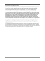
7.6.
3D mapping view
You can use the 3D mapping view as an alternative to the two-dimensional map. Here, the
map is projected onto a head. The setting options correspond to those of the 2D mapping
view. In addition you can rotate the head that is shown. To do this, move the mouse over the
head and hold down the left mouse button while moving the mouse in any direction. The head
will rotate accordingly.
Fig. 7-12: 3D mapping view
Vision Analyzer User Manual
35
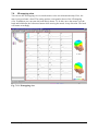
7.7.
Special properties of frequency views (standard, grid and head)
In addition to the properties that were explained above in the sections on standard, grid and
head views, frequency views have some special properties which you can again access
with the Set Display Features button on the tool bar.
Fig. 7-13: Display tab of the Grid View Settings dialog
You can set the following on the Display tab:
•
Ordinate = Voltage or Power (display in μV or μV2)
•
Drawing = Draw Data as Block or Draw Data as Graph
•
Scaling = Logarithmic Scaling (as an alternative to linear scaling)
•
Displayed Range (of frequencies)
•
Show Legend
•
Show Markers
36
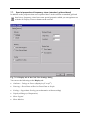
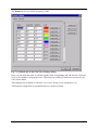
The Bands tab lets you define frequency bands.
Fig. 7-14: Bands tab of the Grid View Settings dialog
Here you can input the name of a band, together with its beginning and end in hertz. Click the
Select Color button to change the color. This brings up a dialog in which you can choose the
color for the band.
Three buttons are available to edit lines: Insert Line, Remove Line and Remove All.
All frequency ranges that are not defined here are shown in black.
Vision Analyzer User Manual
37
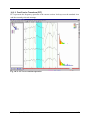
7.8.
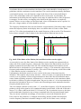
Block markers and transient transforms
If you press the left mouse button somewhere between the channels in the standard view, a
bluish green block marker becomes visible. If you hold the mouse button down and move the
mouse, the size of the block changes. When you release the mouse button, a context menu
appears with the choice of transforms: Zoom, FFT and Map. These transforms are transient,
i.e. their results are not stored anywhere. They are only intended for visual inspection of the
current data. If you choose one of these transforms, the current data window is split and the
result of the transform appears on the right. This relates to the current block. If you change the
block position by moving the mouse over it, pressing the left mouse button down and moving
the mouse in a horizontal direction, the result on the right is updated accordingly.
Fig. 7-15: Example of a transient transform
In the head and grid views you must move the mouse very close to the displayed signal and
then press the left mouse button in order to activate the block marker.
A vertical tool bar appears on the right edge of the right-hand window, and you can use this to
change the settings for the transient view.
You can change the size of the pane for displaying the transient transforms by using the
mouse to shift the divider bar between the panes (left mouse button).
In order to change the default setting for the page ratio between the two views, choose
Configuration > Preferences... from the menu and then select the Views tab.
38
Here you will find the Default Width of Transient View option at the bottom. Enter the width
of the transient view as a percentage of the overall window width.
Fig. 7-16: Setting the default width of the transient view
Press the ESC key when you want to close the right-hand pane.
Vision Analyzer User Manual
39
7.9.
Overlaying different data sets
If you want to overlay several complete data sets, then you can do it with the Window >
Overlay... menu option. Alternately, you can press the following button on the tool bar:
This option only works for data sets with the same sampling rate and same duration. The
number of channels must not necessarily be identical. The view checks the channel names and
only overlays those which are the same.
The easiest way of overlaying data sets is drag and drop. To do this, use the mouse in the
History Explorer to select the data set that you want to overlay, hold the left mouse button
down and drag the mouse onto the view. Then release the left mouse button. This only works
if the conditions described in the paragraph above are satisfied.
Fig. 7-17: Overlay dialog
This dialog enables you to select one or more data sets from the whole workspace. The
selection is determined by one of four possible criteria which can be set at the top of the
dialog. These are Parent, From Same History File, With Same Name and From All Datasets.
Parent is the data set from which the current data set was calculated. This option is
inaccessible if the current data set represents the raw data EEG.
From Same History File shows all data sets in the current history file.
40
With Same Name lists all data sets in the workspace which have the same name as the current
data set.
Finally, From All Data Sets lists all data sets in the current workspace.
If you select one or more data sets which have the same length and sampling rate as the
current data set, then the channels for the selected data sets appear in overlaid mode. The
Clear Overlays button appears at the top right of the data window. Clicking this button
removes the overlays again.
Vision Analyzer User Manual
41
7.10. Setting markers manually
You can set markers manually in addition to those markers that are already in the data set.
A marker in the Analyzer has five different properties: type, description, position, channel
number and length.
You will find more information on markers in the Annex under "Markers".
In order to set markers, you have to put the data window into marker edit mode. You do this
by pressing the following button on the tool bar:
Marker Edit Mode
Pressing the left mouse button now in the data window brings up a dialog which enables you
to set a marker. You can specify any type and a description. You can also assign the marker to
an individual channel or all channels. If you assign the marker as the Voltage type and assign
it to a special channel, then the current voltage at this point and the time are displayed next to
the description which you can input as an option.
Fig. 7-18: Add Marker dialog
You can also shift markers as long as you are in marker edit mode. To do this, move the
mouse pointer over the marker that you want to shift. Then press the left mouse button, hold it
down and move the mouse. A magenta motion indicator follows the mouse movement. The
marker is shifted when you release the mouse button.
To delete a marker just click it briefly. This opens a menu from which you can choose
whether you want to delete the marker or position a new one.
When you have finished editing markers, you quit marker edit mode by pressing the button on
the tool bar again.
When you close the current data set or perform a transform, the Analyzer will create a new
data set beneath the current one with the name Markers Changed.
42
8. Automation through history templates
As described in the "Getting started and handling" chapter, you can transfer an existing
processing history from one history file to another. You can also store such a history in a
special kind of file named a history template. You can use this template later to apply the
history either to a single history file or to several files automatically.
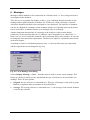
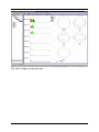
Choose History Templates > New to create a new history template. A window opens in
which there is a single entry named Root. To generate a template, open a history file in which
you have already carried out one or more operations.
Drag a data set of the history file to the root node of the history template. This data set now
appears in the history template together with data sets that have been derived from it. In fact,
only the operation instructions are transferred to the history template, not the data.
Fig. 8-1: Example of a history template
You can edit the history structure in the template in the same way as in a normal history file,
i.e. you can rename and delete nodes. You can also drag individual history nodes from the
open template back onto history files and thus trigger the corresponding operations.
To apply the history template to an entire set of history files, save the current template to a file
with File > Save.
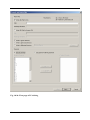
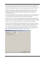
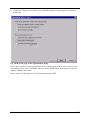
Then choose History Templates > Apply to History Files.... The following dialog appears.
Vision Analyzer User Manual
43
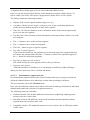
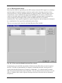
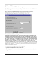
Fig. 8-2: History template application dialog
Your first option in this dialog is to select a history template under Select History Template. If
you have not closed the history template window, then the name of the current history
template appears here. Otherwise click the Select button and pick a history template.
In the next input group (Starting Position in History File(s)) you define whether the template
is to be applied to the initial data set (Root) of the history files or to one of the subsequent data
sets (Choose Data Set). If you choose the second option, enter the name of the data set to
which you want to apply the template. Note that if there are several data sets of the same
name in a history file, only the first one that is found will be taken into consideration.
If you enable the Use Logfile option, then all messages that are usually output in a dialog will
be written to a log file. In this case, all Yes/No questions are automatically set to Yes. This
prevents automatic processing from being interrupted while the program waits for an input.
The log file is displayed when processing has finished.
Now you can choose the history files to which you want to apply the template. You have the
following options here:
•
Primary History Files Only
You can confine the selection to primary history files only.
•
Use Whole Workspace
•
Select Individual History Files
44
•
Selection Filter
With this option you can filter selectable files by name criteria. Wildcards can be used:
"*" for multiple characters and "." for one character. If the Test1H, Test2G and Hest5 files
are in the workspace, then Test* will filter out just Test1H and Test2G. The filter .est*
would accept all three files, etc. When you have set the filter, press the Refresh button to
refresh the selection of available files.
•
Available Files
•
Selected Files
Here, you have a choice of Whole Workspace or Select from List.
The selected history files are processed with the specified operations when you press the OK
button or the Enter key
If a history file has already been processed with the template in question, it is ignored.
Vision Analyzer User Manual
45
9. Macros
A Basic interpreter has been built into the Analyzer so that users can program functions
ranging from simple automation macros to complex applications. This interpreter accesses the
Analyzer via the OLE Automation interface. This interface gives you access to many methods
and properties of the Analyzer, as well as access to every single data point in a data set
(history node) in all history files.
Choose Macro > New to write a new macro. This causes the menu bar and tool bar to change.
In addition, an edit window opens containing the following two lines.
Sub Main
End Sub
You insert the actual macro code between these two lines.
The short macro shown below simply opens all history files, outputs a message and then
closes the files again.
Sub Main
For Each hf In HistoryFiles
hf.Open
Next
MsgBox "All history files are open"
For Each hf In HistoryFiles
hf.Close
Next
End Sub
Fig. 9-1: Macro option dialog
46
When you have input your code, you can test it with the F5 key. You can save the macro with
File > Save and close the edit window. To run an existing macro when you are not in the
macro edit window, choose Macro > Run. You can then choose the macro you want to run.
Alternately, you can make macros appear as items on the macro menu bar. Choose Macro >
Options to do this. Here, you can choose up to 10 different macros. When you have made
your choice and reselected the Macro menu, you will find your macros on the bar. You can
now also access the chosen macros via keyboard shortcuts (Alt-M, 1, 2 , 3...).
Please refer to the "Vision Analyzer Macro Cookbook" and the "Vision Analyzer - Ole
Automation Reference Manual" for more details about writing macros. You can find out more
about the built-in Basic during an editing session by means of Help > Editor Help and Help
> Language Help.
Vision Analyzer User Manual
47
10. Transforms
This chapter alphabetically lists the transform components that currently belong to the
Analyzer in the way they appear on the Transformations menu and in the context menu of a
view after marking a block.
There are three basic types of transforms in the Analyzer. These are primary transforms
which store the nodes in a primary history file, e.g. filters, secondary transforms which
generate secondary history files, e.g. Grand Average, and the transient transforms which
were described in the "View" chapter and whose result is only kept temporarily.
Secondary transforms appear at the bottom of the Transformations menu, kept apart from
primary transforms by a separator.
It is in the nature of secondary transforms that they cannot be included in history templates.
Transient transforms are available when you mark a block as described in the "Views"
chapter.
48
10.1. Primary transforms
10.1.1. Artifact Rejection
After segmentation, the data set can be examined for physical artifacts with this transform.
Segments with artifacts can be removed or marked.
If artifacts need to be marked before segmentation, please use the Raw Data Inspector which
is described later.
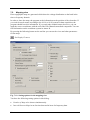
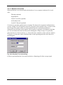
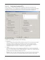
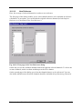
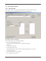
Fig. 10-1: Artifact rejection – first dialog
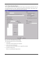
When you select Artifact Rejection from the Transformations menu, the first dialog appears
where you have a choice of three modes:
•
Manual Segment Selection
•
Semiautomatic Segment Selection
•
Automatic Segment Selection
This dialog also includes an item labeled Individual Channel Mode. With this mode you do
not need to reject entire segments but can simply mark individual channels as bad. In this
case, the Average module will later search for as many segments as possible separately for
each channel (also see "Average").
Vision Analyzer User Manual
49
The final option in this dialog is Mark Bad Segments Instead of Removing Them. Here you
define whether bad segments (i.e. with artifacts) should simply be marked instead of removed.
If you do not check this option, the new data set will only contain the remaining segments.
The three segment selection methods are described in detail below.
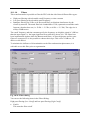
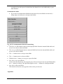
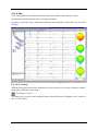
10.1.1.1.
Manual segment selection
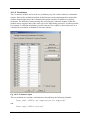
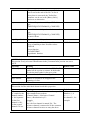
When you press the Finish button, a grid view appears which has a dialog on its right.
If you did not select individual channel mode, you can remove individual segments here.
Fig. 10-2: Dialog for manual segment selection
For this purpose there is a dialog box with the following elements:
•
Display of the current segment number (Segment x of y).
•
A window with the text Remove or Keep indicating what is to be done with the current
segment.
•
The Remove button to include the current segment in the list of segments to be removed
and move on to the next segment.
50
•
The Keep button to take the current segment out of the list of segments to be removed and
move on to the next segment.
•
The << button to move to the previous segment.
•
The >> button to move to the next segment.
•
The Goto... button to go to a specific segment.
•
Remove Segments
The segments that are due to be removed are listed here. You can display a segment by
double-clicking it.
•
Step Only to Kept Segments
If you select this check box, the program goes to the nearest previous segment that is
not in the list of segments to be removed when the << button is clicked. The equivalent
applies to the >> button for subsequent segments.
•
Step Only to Removed Segments
This check box has the exact opposite effect to the previous one.
•
Show Artifacts
This causes the marked artifacts to be displayed.
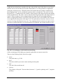
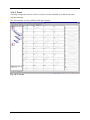
Fig. 10-3: Dialog for manual segment selection in individual channel mode
Vision Analyzer User Manual
51
A slightly different dialog appears if you chose individual channel mode.
Here you can also mark sections directly on the channels as artifacts with the mouse. To
delete a mark, just click it. This opens a popup menu with the Delete Artifact option.
The dialog contains the following elements:
•
Display of the current segment number (Segment x of y).
•
A window with the text No Artifact or Segment with Artifacts indicating whether an
artifact has been marked anywhere in the current segment.
•
The Clear All Channels button to remove all artifact marks in the current segment and
move on to the next segment.
•
The Mark All Channels button to mark all channels as having artifacts and move on to the
next segment.
•
The << button to move to the previous segment.
•
The >> button to move to the next segment.
•
The Goto... button to go to a specific segment.
•
Step Only to Clean Segments
If you select this check box, the program goes to the nearest previous segment that does
not contain any artifact marks when the << button is clicked. The equivalent applies to
the >> button for subsequent segments.
•
Step Only to Segments with Artifacts
This check box has the exact opposite effect to the previous one.
•
Segments with Artifacts
All marked artifacts are listed here. You can display an artifact by double-clicking it.
When you have made your choice, click the OK button.
10.1.1.2.
Semiautomatic segment selection
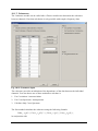
In semiautomatic segment selection the Continue button takes you to a page on which you
define the channels that are to be taken into account when searching for artifacts.
The next step takes you to the Criterion menu.
Here, you can define the artifact criteria which will result in marking of channels in individual
channel mode and in the exclusion of segments otherwise.
The following criteria are available:
•
Gradient criterion: The absolute difference between two neighboring sampling points
must not exceed a certain value.
•
Max-Min criterion: The difference between the maximum and the minimum within a
segment must not exceed a certain value.
•
Amplitude criterion: The amplitude must not exceed a certain value or fall below another
certain value.
52
•
Low activity: The difference between the maximum and minimum in an interval of
selectable length must not be lower than a certain value.
The individual criteria can also be combined.
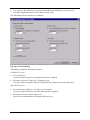
Fig. 10-4: Criteria dialog
The dialog contains the following elements:
Gradient Criterion
•
Check Gradient
If you select this check box, the gradient criterion is applied.
•
Maximum Allowed Voltage Step / Sampling Point
You specify the maximum allowed voltage difference between two data points here.
Max-Min Criterion
•
Check Maximum Difference of Values in the Segment
If you select this check box, the Max-Min criterion is applied.
•
Maximum Allowed Absolute Difference
Specify the maximum allowed voltage difference here.
Vision Analyzer User Manual
53
Amplitude Criterion
•
Check Maximum and Minimum Amplitude
If you select this check box, the amplitude criterion is applied.
•
Minimum Allowed Amplitude
Specify the minimum allowed voltage level here.
•
Maximum Allowed Amplitude
Specify the maximum allowed voltage level here.
Low Activity Criterion
•
Check Low Activity in Intervals
If you select this check box, the Low Activity criterion is applied.
•
Lowest Allowed Activity
Specify the minimum allowed activity here.
•
Interval Length
Specify the interval length within which activity is not allowed to fall below the
minimum.
The Test Criteria button enables you to check the test criteria.
When you have completed the dialog, you still have the opportunity to change the results. The
same view appears with the same setting options as in manual segment selection.
10.1.1.3.
Automatic segment selection
Here, you perform all operations in exactly the same way as for semiautomatic segment
selection. The only difference is that you do not have any opportunity to make corrections.
54
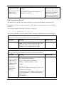
10.1.2. Average
The Average module is used for averaging data which has been segmented. It is used after:
Filtering (optional)
Segmentation
Ocular Correction (optional)
Artifact Rejection
Local DC-Detrend (optional)
Baseline Correction
Note that criteria – such as marker types, exclusion of segments with incorrect patient
responses and the like – are defined in the Segmentation module and not here.
With the Average module you can average either all segments or one chosen range.
You can also specify whether you only want to average segments with odd numbers (segment
1, 3, 5, ...) or even numbers (2, 4, 6 ...).
Another important option is individual channel mode. Here, the program no longer assumes
that all channels for every segment are to be included in averaging but that each channel can
be considered on its own. If only one channel in a segment has been marked as bad, all other
channels are used in averaging nevertheless. The result is that the number of segments
included in averaging can be different for each channel. To use individual channel mode, you
have to make preparations in various preprocessing steps:
•
If you use the Raw Data Inspector make sure that you also enable individual channel
mode here. You can find more details on this in the "Raw Data Inspector" section.
•
As far as segmentation is concerned, you must not suppress bad intervals (also see the
"Segmentation" section).
•
If you use the Artifact Rejection module in place of or in addition to the Raw Data
Inspector, then you must also use individual channel mode here in order not to reject
entire segments but to mark channels only (also see the "Artifact Rejection" section).
You can output the standard deviation as an additional data set.
The signal-to-noise ratio (SNR) of the data to be averaged can also be calculated.
The SNR provides a measure of the quality of the EEG signal. Since neither the signal nor
the noise in the EEG is known exactly, your average total powers must be estimated with
statistical methods.
In this process the average noise power of the EEG is calculated for each channel first. It is
assumed that noise will be eliminated by averaging. Thus average noise power is calculated
from the total of the squares of the differences between the EEG value and the average value,
divided by the number of points minus 1.
Vision Analyzer User Manual
55
In order to ascertain the average power of the signal in the EEG, you first calculate the total
power of a channel of the EEG. This is a result of the mean of the squares for all data points
of the channel before averaging.
It can be assumed that the signal and noise are uncorrelated. Consequently the average power
of the signal is equal to the difference between the average total power and the average noise
power.
The SNR is then calculated from the quotient of the average signal power divided by average
noise power.
The result of SNR calculation is stored in the resultant history node as a description. You can
see the result and other information by moving the mouse pointer over the corresponding icon
or over the view and pressing the right mouse button. A context menu appears which contains
the Operation Infos item among other things. Choose this item. A window opens showing
information on the transform that has been performed.
Fig. 10-5: Average dialog
The Average module displays a dialog box at the start.
You can make the following settings:
Segment Range
Here, you can specify the time range whose segments are to be included in averaging. The
number of segments available is displayed. You have the following choices: Use Full Range
and Specify Range of Segments.
•
Individual Channel Mode
If you do not select this mode, all segments which have a Bad Interval mark at any point
are rejected completely.
•
Odd - Even
Here you define whether you want to perform averaging on the basis of odd or even
numbers. The segments determined by the time range act as the basis for the count.
56
•
Statistical Data
Here you define whether you want to output standard deviation as a new data set, and
whether you want to calculate the signal-to-noise ratio.
Vision Analyzer User Manual
57
10.1.3. Averaged Cross Correlation
This transform enables you to calculate the averaged cross correlation between two channels
on a segmented EEG. It is a statistical measure of the dependency of two channels. Timeshifted and frequency-shifted dependencies are also calculated. If this transform is applied to
complex data, the complex cross correlation is calculated.
Fig. 10-6: Averaged Cross Correlation dialog
The calculation procedure is as follows:
•
58
First, the cross correlation between the specified pairs of channels is calculated segment
by segment using the following formula:
CrCorr(c1, c2)(j) = Σi (c1(i) – Avg(c1) ) (c2 (i+j) – Avg(c2) )* / ( StdDev(c1) * StdDev(c2) ),
i = 1,..., segment length, j = 1-segment length, ..., segment length,
Avg: average of all the values in the segment,
StdDev: standard deviation of all the values in the segment..
The value 0 is added to the channels for the purpose of calculation outside the segment.
•
Then an average is formed across all segments for each of these pairs.
When this transform is applied to the data in the frequency domain, it is also possible to input
a frequency band to which the calculation should be confined. In the dialog, select the
channels between which you want to calculate the cross correlation, and the frequency band if
you are operating with data in the frequency domain. Here, you also have the option of
selecting the entire frequency range. To calculate the auto correlation of a channel, specify its
channel name both in the left and right list box of a row in the input table.
As the result, you get the channels in which the average of the cross correlations are recorded
for the time or frequency shift.
Vision Analyzer User Manual
59
10.1.4. Band-rejection filters
Band rejection filters are generally used in EEG analysis when the EEG signal is overlaid by a
spurious signal of constant frequency. Spurious signals on the electricity network or from
electrical activities of poorly shielded monitors are typical examples. Whereas these sources
of interference can be eliminated by improving shielding there are sources of interference
which are inevitable when acquiring EEGs. For example a spurious signal is generated as a
result of magnetic field changes when an EEG and MRI in the EEG are acquired
simultaneously. These spurious signals have typical frequencies and can largely be eliminated
by a combination of low-pass filters and band rejection filters.
There are two steps in the wizard for the Band Rejection Filter module:
Fig. 10-7: First step in the Band Rejection Filter wizard
In the first step you can define any number of band rejection filters that you want to apply to
the EEG. The filter is determined by its frequency, bandwidth and order. In this process a
signal at the threshold frequencies (frequency ± bandwidth / 2) is reduced to half its amplitude. The order determines the slope of the filter. You can choose between an order of 2 or an
order 4. A higher order results in greater filtering in the interval between the two threshold
frequencies.
60
In the second step in the wizard you can select those channels that you want to apply the filter
to. In this way you can, for example, exclude control signal channels which have not been
contaminated by spurious signals from filtering. It is possible to apply various band rejection
filters to different channels by using this module several times.
Fig. 10-8: Second step in the Band Rejection Filter wizard
Vision Analyzer User Manual
61
10.1.5. Baseline Correction
With the Baseline Correction module, the baseline of every segment is adjusted. It is used
after:
Filtering (optional)
Segmentation
Ocular Correction (optional)
Artifact Rejection
Local DC-Detrend (optional)
Correction is generally applied before averaging. The interval in a segment is defined whose
average voltage level corresponds to the new zero point of the segment values. In other words,
the average of the points of the previously defined interval is ascertained, and this is
subtracted from all points in the segment. This operation is applied to all channels in the data
set. You can choose the interval to be used in forming the voltage average. It is generally
placed in the area of lowest activity, i.e. best of all before stimulus or other reference markers.
To do this, you enter the values in milliseconds for the beginning and end of the interval in
the dialog box.
Fig. 10-9: Baseline Correction dialog
Failure to perform Baseline Correction can lead to a flattening off of the average signal.
62
10.1.6. Change Sampling Rate
This transform allows you to change the sampling rate of a data set.
The dialog displays the current sampling rate (Current Rate) and allows you to enter a new
rate.
Fig. 10-10: Change Sampling Rate dialog
The conversion is carried out by means of a cubic spline interpolation (third-degree
polynomial). Please note that the length of time required for the EEG is generally reduced by
several milliseconds when this method is used, since the polynomial cannot be calculated up
to the edges of the original data set. You should therefore carry out the conversion in the raw
EEG.
Vision Analyzer User Manual
63
10.1.7. Coherence
The Coherence module can be called after a Fourier transform to determine the coherence
between channels. Note that calculation is only possible with complex frequency data.
Fig. 10-11: Parameter input
The coherence provides an indication of the dependence of the data between the individual
channels. You can choose one of three methods to calculate it:
1. Use Correlation / Autocorrelation
2. Use Cross-Spectrum / Autospectrum
3. Calculate Only Cross-Spectrum
The first method calculates the coherence using the following formula:
Coh(c1, c2)(f) = | Cov(c1, c2)(f) |² / ( | Cov(c1, c1)(f) | | Cov(c2, c2)(f) | ),
in conjunction with
64
Cov(c1, c2)(f) = Σ (c1, i (f) – avg(c1 (f)) ) (c2, i (f) – avg(c2 (f)) )*.
In the second formula, totaling is carried out via the segment number i. Formation of the
average also relates to segments with a fixed frequency f and a fixed channel c.
The second method uses the cross-spectrum instead of covariance. The formula is as follows:
Coh(c1, c2)(f) = | CS(c1, c2)(f) |² / ( | CS(c1, c1)(f) | | CS(c2, c2)(f) | ),
in conjunction with
CS(c1, c2)(f) = Σ c1, i (f) c2, i (f)*.
Here, too, totaling is carried out via the segment number i.
The third method only calculates the cross-spectrum, which is specified in the formula with
CS.
In methods 1 and 2, values between 0 and 1 are obtained for each frequency and each channel.
In method 3, complex values are obtained, but only the amount is output. When you use this
module you have the choice of including all possible combinations of channels in the
calculation or permitting just a selection of combinations.
If you opt for individual combinations, you can input the combinations of channels in the
table.
Alternatively, select a channel on the left-hand side of the dialog box. When you click the
Combine Channel with All button, all combinations of the selected channel are inserted in the
table.
If the Use Paired Channels View check box is selected, the result is presented in a view that is
split into two parts. On the left, you see graphs in the frequency domain which represent the
coherence calculated for every frequency point and every channel combination. On the right
you see the coherence figures between the channels in the shape of lines. Their coloring codes
the coherence from 0 to 1. If the check box is cleared, the result is displayed in one of the
frequency views.
Vision Analyzer User Manual
65
Fig. 10-12: Output of coherence data
66
10.1.8. Covariance
The Covariance module can be used as a preliminary step for various coherence calculation
options. Most of the methods described in the literature can be implemented in conjunction
with the formula interpreter. More detailed information on this is available in a separate
document. The difference between using this and using the Coherence module is that this
module always supplies data of the same type as the input being processed. It is thus possible,
for example, to calculate and further process coherence for complex-valued coherence or to
calculate the correlation of channels in the time domain.
Fig. 10-13: Parameter input
The two methods of covariance calculation are described by the following formulas
Cov(c1, c2)(x) = 1/N Σ (c1, i (x) – avg(c1 (x)) ) (c2, i (x) – avg(c2 (x)) )*.
and
Cov(c1, c2)(x) = 1/N Σ c1, i (x) c2, i (x)*.
Vision Analyzer User Manual
67
You can use the Subtract Average button to specify whether the first or second method is to
be used to carry out the calculation. In both formulas, totaling is carried out via the segment
number i, and the average value obtained applies to the segments at a fixed time or at a
frequency of x and a fixed channel c.
If you use this module, you can choose whether you want to include all the possible
combinations of channels in the calculation (Calculate Covariance of All Combinations of
Channels) or whether you only want to permit a selection of combinations (Select
Combination...).
If you decide on individual combinations, you can enter the channel combinations in the table.
Alternatively, select a channel from the list on the right. If you click the Combine Channel
with All button, all the combinations of the selected channel are added to the table.
68
10.1.9. Comparison
With this module, two data sets or two channels of a data set can be compared with each other
after averaging. The Comparison module currently supports the following compare
operations:
Difference waves
Cross correlation
If the operation is performed on two data sets, the data set that is currently displayed is
regarded as the reference set. This means that the new history node is appended to the current
data set. It is important for the comparative data set to have the same sampling rate.
Fig. 10-14: First page of the Comparison module
The first page of the Comparison dialog gives you a choice between calculating difference
waves, cross correlation and lateralized readiness potential.
On the second page you define whether you want to perform the comparison within the
current data set (Compare Channels) or between two data sets (Compare Data Sets).
Fig. 10-15: Second page of the Comparison dialog
If you opt to compare channels, the next page shows a channel menu on which you can select
groups of channels which are subtracted from each other.
Vision Analyzer User Manual
69
Fig. 10-16: Third page of the Comparison dialog when channels are compared
Here, you can also insert a line, remove a line, or remove all lines.
If you opt to compare two data sets, then the page that appears shows a menu for data sets
instead of channels.
You see a list of all history files in the current workspace. You can open them by doubleclicking a file.
70
Fig. 10-17: Third page of the Comparison dialog when data sets are compared
In addition, four buttons are at your disposal to get to the required comparative data set faster:
•
Expand History File
This button expands the current history file.
•
Expand Same Names
This button expands all history files which have a data set of the same name, up to this
data set.
•
Expand All
This button expands all history files.
•
Collapse All
This button collapses all history files again.
Vision Analyzer User Manual
71
If you select the Keep Remaining Channels check box, then all channels which do not contain
an equivalent in the comparative data set are kept anyway.
The Use Relative Path for Template or Drag and Drop option enables you to save the relative
location of the comparative data set. This means that the history templates can always search
for this data set in the same history file.
You can select a data set by double-clicking it or by clicking it once and clicking the Finish
button.
72
10.1.10.
Current Source Density (CSD)
This transform replaces the voltage levels at electrodes by valid head coordinates through the
current source density at these points. The unit is µV/m². The resultant curves
do not have any reference electrodes any more. They can be processed further with other
transforms.
You obtain the current source density by applying the spherical Laplace operator to the
voltage distribution on the surface of the head at a fixed time. Since voltage distribution is
only known at the electrodes, the procedure of spherical spline interpolation is used to
calculate the total voltage distribution. An exact mathematical presentation of this procedure
is given in:
F. Perrin et al. (1989), Spherical splines for scalp potential and current density mapping,
Electroencephalography and Clinical Neurophysiology, 72, 184-187, together with a
correction in Electroencephalography and Clinical Neurophysiology, 76 (1990), 565.
To calculate spherical splines, three parameters are needed which are requested by the
transform in a dialog: the order of the splines (labeled m in the article mentioned above) and
the maximum degree of the Legendre polynomial that is to be included in the calculation. The
interpolation will be flatter or wavier, depending on which values are used for the order.
Interpolation with an increasing order of splines becomes flatter. Basically, the denser the
electrode arrangement, the smaller the order should be. Since an infinite series of polynomials
is included in the calculation, this series must be discontinued at a certain degree. The rule
that applies here is the higher the spline order, the lower the degree of the polynomial at
which calculation is discontinued.
Fig. 10-18: CSD dialog
The Lambda approximation parameter defines the accuracy with which the spherical splines
are approximated to the data to be interpolated. For various mathematical reasons, a Lambda
that is too large or too small leads to an inaccurate representation. Unless there are methodical
exceptions that speak against it, the default value of 1e-5 should be retained.
Vision Analyzer User Manual
73
Despite these rules of thumb it is not advisable to accept the results of this module without
checking them. In the CSD method, various parameters can cause good or bad results in
different data sets owing to approximations and rounding inaccuracies. It is therefore
advisable to proceed as follows when using this module:
•
Before running the CSD calculation, the parameters of the spherical splines should be
checked in the current data set using the mapping view. To do this, generate a mapping
view for the data set and select interpolation with spherical splines using the parameters
that you want to use for CSD calculation.
•
Check, possibly by comparing with interpolation by triangulation, whether the spherical
splines satisfactorily approximate the voltage distribution on the surface of the head. If
not, change the parameters until this is the case.
•
Run the CSD calculation with these parameters and then make sure that the result is
correct by generating a mapping view.
74
10.1.11.
DC-Detrend
This transform calculates the DC trend from the signal.
Two different approaches are taken, depending on whether this transform is called before or
after segmentation.
When called before segmentation, global trend correction is used as described in:
Hennighausen et al. (1993), A correction method for DC drift artifacts,
Electroencephalography and Clinical Neurophysiology, 86, 199-204
Fig. 10-19: Global DC-Detrend dialog
In accordance with this method, in the first step the average voltage is calculated for each
prestimulus interval of the specified marker type. In the second step, the average voltage is
calculated for every DC reset in an interval directly before DC reset. The difference between
this average voltage before DC reset and the average voltage of the first prestimulus interval
after this DC reset is added as an offset to all voltage levels after this DC reset. Then, in the
third step, all average values that have been calculated for the prestimulus interval and
corrected by adding the offset are viewed along the time axis, and the trend is ascertained by
applying linear regression to this data. Only intervals which do not contain any DC reset are
included in the calculation. In the fourth step, the trend is subtracted from the original data,
taking the DC offset into account.
You can input the following parameters for this algorithm.
•
The interval length in milliseconds or data points
•
The data type of the markers for which the prestimulus intervals are calculated, and the
length of these intervals.
Vision Analyzer User Manual
75
•
The length of the intervals before DC corrections for which the voltage averages are to be
calculated for the following data, together with the resultant offset.
If this transform is called after segmentation, then local DC trend correction is applied. Here,
a linear function is subtracted from the data from every segment. The slope and boundary
values of this linear function are calculated for every segment from a certain interval at the
beginning and at the end of the segment.
In the DC-Detrend dialog, you can specify the intervals based on time or data points.
To minimize the influence of DC trends on ocular artifact correction, it is advisable to
perform DC trend correction before ocular artifact correction.
Fig. 10-20: Local DC-Detrend dialog
76
10.1.12.
Edit Channels
This transform enables channel information to be edited. Editing comprises the following
aspects:
•
•
•
Hiding channels
Changing the channel and reference channel names
Changing position details
Fig. 10-21: Edit Channels dialog
The dialog shows the following fields for all channels from left to right:
•
# (channel number): This cannot be edited.
•
Org. Label (original name of the channel): This cannot be edited.
•
Enabled: Deselect this check box to hide the channel in question.
•
Chn (+) (channel name): This can be changed as required.
•
Chn (-) (reference channel name): This can also be changed as required. Changing the
name does not cause any rereferencing. The name is for information purposes only.
•
Radius, Theta, Phi (position details): Please refer to the "Electrode coordinate system"
part of the Annex for more information on this.
Vision Analyzer User Manual
77
On the right of the dialog you will also see the Default Pos. button. This button sets all
electrode coordinates to the 10/10 or 10/20 system, depending on the channel names, after
asking if you really want to do this. All unrecognized channels are set to position 0,0,0
(invalid position).
78
10.1.13.
Fast Fourier Transform (FFT)
In the course of a Fourier transform, data is transformed from the time domain to the
frequency domain, i.e. the resultant items of data indicate the extent to which the individual
frequencies are present in the EEG between 0 Hz and at most half the sampling rate.
Fig. 10-22: FFT dialog
You have the following input options in the FFT dialog:
•
Resolution
Here you define the resolution of the new data set in hertz. You can choose between the
maximum resolution resulting from the number of points in the segments and the
sampling rate and any resolution that you decide to set. The maximum resolution is
calculated as follows: resolution = sampling rate / segment length.
•
Output
Here you define the type of the resulting data and the unit to be used in calculating the
data. You can choose between the following data types: voltage in μV, voltage density in
μV/Hz, power in μV2 and power density in μV2/Hz.
Density: In the case of the voltage density and power density functions, the spectral line
values are scaled as if they were calculated with spectral line spacing of 1Hz, which
Vision Analyzer User Manual
79
permits comparisons between FFT analyses that have been carried out with different
spectral resolutions. To this end, the spectral line values are multiplied by a constant
factor b, which corresponds to the reciprocal value of the spectral line spacing (b=1/fb).
Normalize: Another kind of comparability of FFT data can be achieved by means of the
Normalize Segments check box. It is often important in EEG research to draw
comparisons by changing the spectral composition of the EEG signal, but since the total
power of the EEG varies from segment to segment, such comparisons are not normally
carried out. By means of the Normalize function, however, it is possible to normalize the
total area in the entire EEG spectrum or in only a part of it and thus make it comparable.
If you do not select Normalize mode, the FFT module returns data in the frequency range
in the way it is generated by a Fourier transform. Selecting Normalize causes the data to
be multiplied after the Fourier transform by a factor which makes the area under every
channel and in every segment identical. In this case, it is not the absolute data that is
output but the relative distribution of activity on the individual spectral lines.
To this end, the lower and upper limits of the normalization range can be specified in two
dialog boxes. The minimum lower limit is fixed at 0.5Hz, since it is generally assumed
that frequencies under 0.5Hz are not electrocortical in origin and that these frequencies are
extremely unstable from segment to segment. The area of this frequency range is
calculated and set to the area value of 100 by multiplying it by a normalization factor that
differs from segment to segment and channel to channel. In the same way, all of the
spectral line values that are not within the normalization range are multiplied by this
factor and thus also normalized.
Band comparisons such as the relative alpha share of the EEG or the alpha slow wave
index can thus be calculated easily. Normalization also makes it much easier to calculate
the spectral corner frequency, for example.
Full spectrum: The Use Full Spectrum check box is used to specify whether only one or
both halves of the spectrum is/are to be used to calculate the spectral line values. If both
are used, this effectively doubles the spectral line values. This is of particular significance
when power spectra are calculated, since this check box allows both of the definitions of
spectral power (µV² or as µV²/2) used with EEGs to be taken into account. If you select
the Use Full Spectrum check box, the resulting FFT power spectra behave in accordance
with the Parseval theorem, which states that the total power in the power spectrum should
also be equal to the total variance in the time signal.
Complex output: You can use the Produce Complex Output check box to specify
whether the FFT module is to supply complex data. You should generate complex data
whenever you want to further process the data resulting from the FFT with transforms that
have to process not only the values of the spectral lines but also their phase information
and consequently require complex data. Coherence analysis is an example of this.
•
80
Data Window
Here you can define the FFT data window. You can choose between the window types No
Window (no window or rectangular window) Hanning Window and Hamming Window.
You can also input the window length as a percentage of the segment length. The window
function is presented graphically (see below for information on the window function).
•
Data Compression
Here, you can specify whether you want to store the data in compressed or uncompressed
format. Compressed data saves storage space in the history file but is less accurate than
uncompressed data. If you opt for compressed data, you can choose the degree of
resolution in nanovolts (1000 nV = 1 μV). The lower the resolution of the data (higher
values), the greater the compression effect. Consequently less storage space is required.
The procedure:
Strictly speaking, a Fourier transform extends from 0 Hz to the maximum sampling rate, but
the data in the high frequency range results from conjugate-complex values from the data in
the lower frequency range is therefore not calculated explicitly.
The data values are scaled in such a way that a sine wave of 1 Hz and an amplitude of 100 µV
generates a value of 50 µV at the 1 Hz position when the output format is Voltage, calculation
takes place without a data window, and the Use Full Spectrum check box is not selected.
Together with the corresponding data value in the high frequency range (i.e. when the Use
Full Spectrum check box is selected), this results in the original value of 100 µV. This
approach corresponds to the calculation of a Fourier transform with subsequent division by
the number of data points used.
Brief information about interpolation:
Although the Fourier transform can in principle be used at any point in the process, its use is
recommended on segmented EEGs to save time.
The transform is executed separately for each segment. It is not essential for the number of
data points in a segment to be a power of 2. If it is not a power of 2, the segments are
automatically extended to the next higher power of 2, and the corresponding number of zeros
are added to the existing data.
This process, which is also known as padding, corresponds to the interpolation of the data in
the frequency spectrum of the original data set. As a result, a frequency spectrum is obtained
that has a higher resolution than the original data set. No data is lost here, however, and the
data that results from this process does not contain any artifacts.
On account of the interpolations, however, it cannot be expected that using this process on
data with any segment length and sampling frequency will always provide comparable results,
since the FFTs calculated in this way differ in terms of the total number of data points and
thus also in terms of the information content of the original input data, which inevitably leads
to differences in the resulting spectra. Interpolated FFT spectra are thus suitable, above all, for
visual data inspection.
To avoid the interpolation of the FFT data at all resolutions, you should thus ensure that the
number of data points in the segments is a power of two and select the Maximum Resolution
option in the module.
If you select a different resolution in the FFT module to the maximum spectral resolution
determined by the segment length and data rate, the resulting FFT spectra are also interpolated
or even interpolated and integrated, depending on the selected resolution. As mentioned
above, interpolation like this always results in correct FFT spectra and does not create any
Vision Analyzer User Manual
81
artifacts, but it is important to remember that an FFT analysis like this cannot necessarily be
compared with an FFT analysis using a data set that has the resolution selected here as the
maximum spectral resolution.
To illustrate this, let’s take an example of an EEG with a sampling rate of 1024 Hz and
segments of 4096 points. The maximum spectral resolution is thus 0.25 Hz (1024/4096=0.25).
If you select the Other Resolution option and enter 1.0 Hz, instead of 1024 data points being
included in the analysis, as would be the case given a maximum resolution of 1.0 Hz
(segments of 1024 data points and a sampling rate of 1024 Hz), four times that number of data
points are involved. The resolution of 1.0 Hz is now established by integrating four spectral
line values. If the resolution ratios are not exactly divisible, the overlaps of the values at the
spectral line edges are interpolated. However, since the original segments are four times
longer and thus inevitably have a different information content to the short segments, in spite
of the FFT resolution theoretically being identical, the results can by no means be expected to
be the same.
It should be stated clearly here that this is not a problem caused by the method used; it is an
inevitable result of the differences in the quantity and contents of the information included in
the FFT analysis when there are different spectral resolutions.
This problem, which is inherent in interpolation, applies in particular to the calculation of
complex FFT values when a resolution other than the maximum spectral resolution is
selected. This is because in this case not only the values of the spectral lines but also their
phase information have to be interpolated and/or integrated. This can impair the flow of the
phase information, which is actually rather steady, and make the result of a subsequent
coherence analysis appear questionable.
To conclude, it is worth repeating that spectra interpolated like this are suitable above all for
the visual inspection of data and should not form the basis for subsequent calculations.
Brief description of how the data window works
In a Fourier transform, it is assumed that the output signal is repeated periodically. Since this
condition is generally not given when EEG sections are transformed, the difference between
the voltage level at the beginning of the segment and the voltage level at the end
of the segment is included in Fourier transform calculations as the point of jump
discontinuity, and causes the data to be corrupted. To reduce this effect, it is possible to lay a
data window over the segment to be transformed. This data window damps the EEG data at
the ends. When the data window has been applied, the voltage level at the beginning and end
of the segment is 0, and rises to the original measured value at the middle of the segment. The
range in which the data window is to be used can be specified in percent. 100% would mean
that only the value in the middle of the segment matches the original data value, and all other
values are damped by the data window. The lower the percentage that is specified, the smaller
the range that is changed by the data window. This principle is represented graphically and
very clearly in the FFT module.
The Hanning window is calculated in accordance with the following equation:
WP = 0,5(1 – cos(2π x/P)),
82
The Hamming window is calculated in accordance with the following equation:
WP = 0,54 –0,46 cos(2π x/P)).
P signifies the above-mentioned percentage. Corresponding symmetric equations apply to the
end of the segment.
It follows from the way in which the data window works, as described above, that the overall
signal and thus the total variance of the EEG signal are weakened by the window, particularly
toward the edges. Accordingly, the use of a data window also results in the damping of the
data produced by the Fourier transform.
For this reason, before the Fourier transform is applied, a correction factor for the data
window and window width used is calculated and used to multiply the data after the Fourier
transform. This correction ensures that the total variance of the transformed signal matches
the total variance of the original signal.
Vision Analyzer User Manual
83
10.1.14.
Filters
This transform makes it possible to filter the EEG with the aid of three different filter types:
•
•
•
High-pass filtering with selectable cutoff frequency or time constant
Low-pass filtering with selectable cutoff frequency
Bandpass filtering for 50 Hz or 60 Hz (notch filter) to eliminate interference by the
electricity network. The notch filter has a bandwidth of 5 Hz, symmetric around the notch
frequency that has been set (i.e. 50 Hz +/- 2.5 Hz, or 60 Hz +/- 2.5 Hz). The edge rise is
always 24 dB/octave.
The cutoff frequency and time constant specify the frequency at which the signal is 3 dB less
than the input signal, i.e. the input signal has been reduced by about 70%. The filters have
been implemented as phase shift-free Butterworth filters. As far as high-pass and low-pass
filters are concerned, it is also possible to choose their slope. This can be 12 dB/oct., 24
dB/oct. or 48 dB/oct.
To minimize the influence of discontinuities on the filter and transient phenomena, it is
advisable to use this filter prior to segmentation.
Fig. 10-23: Filters dialog
You can set the following items in the Filters Dialog:
High-pass filtering (Low Cutoff) and low-pass filtering (High Cutoff):
•
84
Enable:
This turns the filter on/off.
•
Frequency / Time Constant:
This defines the cutoff frequency or, as an alternative with high-pass filtering, the time
constant.
•
Slope:
This defines the slope of the filter.
Bandpass filter:
•
Enable:
This turns the filter on/off.
•
Frequency:
This defines the cutoff frequency (50 or 60 Hz)
If you select the Enable Individual Channel Filters check box, the filters can be set separately
for each channel in the table below the check box. Clicking the Fill Table with Values from
Above button causes the values entered above to be written to the table. You can then change
the channels that need to be filtered differently.
Vision Analyzer User Manual
85
10.1.15.
Formula Evaluator
This module enables new channels to be calculated as functions of existing channels.
Extensive mathematical options are available.
Fig. 10-24: Formula Evaluator dialog
Formulas are input in a dialog. You enter the name of the new channel containing the data
from the calculation in the left column (Name). In the middle column (Formula) you input the
formula that you want to use in calculating the data. This is largely case-insensitive, i.e. no
distinction is generally made between uppercase and lowercase. In the right column (Unit)
you can specify the unit for the new channel. You can save formulas in ASCII files by
clicking the Save to File... button, and import ASCII files containing formulas into the dialog
by clicking the Load from File... button. If you want to create ASCII files with an editor or
other program, every line in the file must be in the following form:
Name = Formula
With the Keep Old Channels option you can keep old channels from the previous data set,
which have not been redefined, without any changes. In this case, you can select New
Channels on Top to ensure that the new channels are placed at the beginning.
There are the following options for formulas, and they can be combined:
•
The operators +, -, * and / as well as parentheses. Mathematical rules of precedence are
observed.
•
Channel names – these are interpreted point by point.
86
•
The constants e, pi and i (imaginary unit) as well as numeric inputs.
•
The mathematical functions sqrt (square root), abs, ln (natural logarithm), log (logarithm
to base 10), sin, cos, tan, atan, sinh, cosh, tanh, real (real part), imag (imaginary part), arg
(argument of a complex number).
•
The shift function (this will be explained in more detail later).
The Formula Evaluator processes both real and complex data but the format of the output data
must be identical to the format of the input data. Real numbers are converted into complex
numbers automatically if necessary. The mathematical functions are currently available for
real arguments only.
Numeric constants are interpreted as a fixed number across the entire range. Channel names
are interpreted point by point. The shift function can be applied to channel names. It has the
following form:
shift(channel, shift-index).
The shift index can be positive or negative. This function is regarded as a left shift, i.e.
shift(Fp1, 1) shifts Fp1 in such a way that the data point which has index 2 becomes the data
point with index 1. Accordingly with shift(Fp1, -2), for example, the data point which has
index 1 becomes the data point with index 3.
Examples:
Many functions in existing modules can also be calculated with the aid of the Formula
Evaluator:
Linear derivation can be calculated with a formula like this:
channel = a*channel 1 + b*channel 2 + ...
RMS of Fp1, Fp2 and Fz can be calculated with the following formula:
RMS = sqrt((Fp1*Fp1 + Fp2*Fp2 + Fz*Fz) / 3)
Similarly, other measures can also be defined here.
Rectify can be defined with
channel = abs(channel)
It is also possible to implement simple filters such as sliding averages with the aid of the shift
function:
Fp1 = (shift(Fp1, -1) + Fp1 + shift(Fp1, 1)) / 3
or
Fp1 = shift(Fp1, -1) * 0.25 + Fp1 * 0.5 + shift(Fp1, 1) * 0.25
If your channel names are numeric, place them in quotation marks in the formula. Here is an
example:
1 = (shift("1", -1) + "1" + shift("1", 1)) / 3
Vision Analyzer User Manual
87
10.1.16.
Frequency extraction
Frequency extraction works on the principle of complex demodulation. In this process, the
EEG signal is transformed continuously by mathematical methods so that the resultant signal
only consists of those component frequencies that lie in the defined range.
In contrast to a Fourier transform, only a specific frequency range can be extracted. The
advantage of this transform is that it also works at high speed with unsegmented EEGs and
the output of each channel is a continuous channel again.
This transform is not to be confused with bandpass filtering. The resulting signal is not the
filtered input signal, but it describes the power or phase of the selected frequency range at any
time.
There are the following input options for the transform object: choice between output of the
power or the phase, and choice of the frequency range to be extracted.
Fig. 10-25: Frequency Extraction dialog
If you opt to output the power, the average power in the specified frequency range is
calculated for each data point. If the phase is chosen, then it is the phase of the signal in the
specified frequency range that is calculated. This number is only defined uniquely up to a
multiple of 2π. When different intervals are chosen, the output values can therefore vary by
multiples of this value. It is possible to infer the dominant frequency in the calculated
frequency range on the basis of the phase. A rising phase indicates a dominant frequency
beneath the middle of the chosen interval, whereas a falling phase indicates that the dominant
frequency lies above the middle of the interval.
88
10.1.17.
ICA (Independent Component Analysis)
This module is used for calculating the ICA of EEG signals, i.e. splitting the signals up into
independent components using information theory methods.
Methods
The object of ICA in what is referred to as “blind source separation” is to reconstruct source
signals from a mixture of such signals. In this case, both the source signals and the mixture
are not known. However, assumptions are made regarding the signals and the mixture of these
signals. In terms of the signals to be reconstructed, it is assumed that they are statistically
independent of one another. More details of the theory used can be found in [BS95], [Car98]
and [MBJS96], so these will not be explained further at this point. It is only important to bear
in mind here that ICA is a purely statistical, i.e. mathematical, process. The process is based
on the aforementioned assumptions and does not use any additional physiological information
whatsoever. It is the responsibility of the user of the module to check whether the assumptions
are met and whether it is possible to do without physiological boundary conditions. The
meaningfulness of the results generated using ICA depends on this check.
The result of ICA is a set of components that are defined in the time domain in the same way
as EEG channels. Furthermore, ICA produces a transform matrix by means of which the
components can be calculated from the channels. The weight matrix is determined using the
Infomax algorithm, an iterative gradient process that is described in [MBJGS97], for example.
Parameter settings
In the first step of the parameter dialog, you can save the matrix used for calculating the ICA
components from the original channels. The matrix is saved as an ASCII file. The same thing
is possible for the inverse ICA matrix. These matrices can then be manipulated and evaluated
using macros and external programs. They can also be used for processing in the Linear
Derivation module. The matrices can be written into the export folder of the Analyzer (for
evaluation), into the raw data folder (for importing into Linear Derivation) or into any other
folder.
In the first step of the dialog, it is also possible to select whether all channels or only a subset
should be used for calculating the ICA. In this way, for example, trigger channels can be
masked out from ICA since as a rule they do not satisfy the aforementioned criteria.
ICA is a statistical process, which means there is no absolute need to use the entire data set
length for calculation. Often, certain areas in the EEG signal can be even more meaningful in
terms of the components. For this reason, the second step in the dialog offers you the chance
to restrict the area of the EEG that is used. On the one hand, this is in order to restrict the
calculation to statistically significant areas while improving the performance of the process on
the other hand.
Vision Analyzer User Manual
89
Fig. 10-26: First page of ICA dialog
90
References
[BS95] A.J. Bell, T.J. Sejnowski, An information-maximation approach to blind separation
and blind deconvolution, Neural Computation 7:1129-1159
[Car98] J.-F. Cardoso, Blind Signal Separation: Statistical Principles, Proceedings of the
IEEE, 86/10, 1998
[MBJS96] S. Makeig, A.J. Bell, T.-P. Jung, T.J. Sejnowski, Independent Component Analysis
of Electroencephalographic Data, Advances in Neural Information Processing Systems, MIT
Press, Cambridge MA, 8, 1996
[MBJGS97] S. Makeig, A.J. Bell, T.-P. Jung, D. Ghahremani, T.J. Sejnowski, Blind
separation of auditory event-related brain responses into independent components, Proc.
Natl. Acad. Sci. USA, 94:10979-10984, 1997
Vision Analyzer User Manual
91
10.1.18.
Level Trigger
This transform enables you to set a marker of the Threshold type on one or more channels
when the voltage exceeds or falls below a certain level. These markers can be used as a basis
for segmentation.
One application would be, for example, muscle activities which are to be used as a reference
in averaging.
Another application would be the use of an analog channel as memory for stimuli in
acquisition systems which do not have digital inputs. Here, different stimuli can be coded as
different voltage levels.
Fig. 10-27: Level Trigger dialog
You have the following setting options in this dialog:
•
Name
Here, you specify a name for the threshold in question.
•
Threshold
You input the threshold in μV in this box.
•
Direction
A list box enables you to specify the direction of the voltage shape which sets the marker
when the threshold is reached. Positive means that the marker is set when voltage is rising
and the threshold is reached. Negative sets the marker when voltage is falling and the
threshold is reached.
•
Channel
Here you select the channel on which the threshold is to be searched for.
•
Reset Value
The value to reset the trigger in µV. It is normally identical to the threshold but can be set
to another value for certain purposes. In a positive direction, the value has to fall below
92
this value before a new trigger of this kind is found. Analogously, the same applies to a
negative direction.
The dialog also incorporates three buttons: One to insert a line, one to remove a line and
another to remove all lines.
Under Time Tolerance you can specify an interval within which triggers of the same direction
in the same channel are not distinguished. If several thresholds within this interval are
exceeded, only the maximum threshold is detected and only one marker is set. The same
applies analogously when values fall below several thresholds within the tolerance. The size
of the interval should be adjusted to the steepness of the edges of the trigger channels.
Vision Analyzer User Manual
93
10.1.19.
Linear Derivation
This transform enables you to generate new channels from linear combinations of existing
channels. The new channels are calculated from coefficients and are assigned to existing
channels according to the following equation:
New channel = Coeff1 * Channel1 + Coeff2 * Channel2 + ....
You can input these coefficients in a matrix, and also store/load them.
Fig. 10-28: Linear Derivation dialog
The dialog contains the following elements:
•
Keep Old Channels
If you select this option, the old channels are included in the new data set as well, i.e. the
new channels are practically additional channels. Otherwise the new data set consists of
new channels only.
•
New Channels on Top
If you select this option, the new channels appear in front of all the other channels.
•
Number of New Channels / Refresh
Here you specify the number of new channels that you want. The Refresh button then
updates the coefficient matrix.
•
Load from File...
With this button you can load a coefficient matrix from a text file if you want to.
94
•
Save to File...
Press this button if you want to save a coefficient matrix that you have input.
If you want to read in a self-generated matrix text file, then it must have the following
structure:
Channel1 Channel2 Channel3 ...
New1 Coeff. Coeff. Coeff.
New2 Coeff. Coeff. Coeff.
The decimal places of the coefficients have to be set as a point (".").
Vision Analyzer User Manual
95
10.1.20.
Lateralized readiness potential (LRP)
This module calculates the lateralized readiness potential (LRP) from two data sets, for
example movements with the left and with the right hand).
To do this, first generate two data nodes. The one node should be segmented after the first
condition (e.g. movement with the left hand) and the second node after the second condition
(e.g. movement with the right hand). Then you should apply an average to these two nodes.
Fig. 10-29: Selection dialog for the second data set
The LRP module then calculates the lateralized readiness potential and writes the result in
new channels which have a name in the form LRP(., .). To run this calculation, you must first
select the path of the second data set in the dialog.
The structure of the selection tree in the dialog is like the Analyzer's history tree. You select
the path for the node by clicking the node. You can search for the node by expanding certain
parts of the tree with the buttons on the right edge. You can also use the Keep Channels of
Parent check box to define whether the channels of the parent node should be included in the
new data set or whether the new data set should only consist of LRP data. Double-clicking the
96
selected node or pressing the Next > button takes you to the second dialog in which you can
select the channels for the LRP.
Fig. 10-30: Selection dialog for channels
In calculating the LRP, the module forms the difference between contralateral and ispsilateral
electrodes in the parent node and the reverse difference in the second node, and calculates the
average of these two differences. For this reason, the two left-hand columns of the channel list
are assigned to the first data node (parent) and the two right-hand columns are assigned to the
second data node. It is generally sufficient to fill the two left-hand or two right-hand columns.
The dialog module then searches for the corresponding channels in the other data set and fills
the other columns accordingly when the associated channels have been found and the input
boxes are still empty. This specification can, of course, be changed afterwards. If no suitable
channels are found, all columns have to be filled.
When all columns of the required rows have been filled correctly, pressing the Finish button
concludes input of the channel list and the LRP is calculated. The structure of the LRP
channels is described in the operation info for your information.
Vision Analyzer User Manual
97
Here is a typical sample application to illustrate the input procedure:
In an experiment, a warning stimulus of the test person conveys information on which hand is
to respond to a subsequent imperative stimulus. The warning stimulus, imperative stimulus
and the response (left hand, right hand) are stored as markers in the raw EEG. Using the
Segmentation module in conjunction with advanced Boolean expressions, two segmented data
sets (nodes) are generated. The one node corresponds to the response with the left hand and
the other node to the response with the right hand. You can find more details on this in the
“Segmentation” section of the manual. An average is calculated for the two nodes, and the
average nodes are given meaningful names (e.g. Avg left, Avg right). The LRP data should be
generated as subnodes of the Avg left node. The LRP module is therefore applied to this node,
and the Avg right node is selected as the second data set. Let us assume that the LRP is to be
calculated for channels C3 and C4, i.e. C4 – C3 is calculated for Avg left and C3 - C4 for Avg
right. Then these differences are averaged. Thus C4 is entered in the first column and C3 in
the second column. The corresponding channel names C3 and C4 appear in the third and
fourth columns. After the calculation, a channel appears named LRP(C4,C3) which is the
result of (C4(left) – C3(left) + C3(right) – C4(right)) / 2.
Further explanations of lateralized readiness potential are given in:
Sommer, W., Ulrich, R., Leuthold, H. (1996) Das Lateralisierte Bereitschaftspotential als
psychophysiologischer Zugang bei der Untersuchung kognitiver Prozesse. Psychologische
Rundschau, 47, 1-14
98
10.1.21.
MRI Artifact Correction
This module permits the correction of different types of artifacts that occur during the
recording of EEG signals in a magnetic resonance tomograph. Some of these artifacts are
formed as a result of changes to the magnetic field in the scanner (scanner artifacts). Pulse
artifacts are also created in the EEG channels due to the heartbeat and the resulting blood
pulse in the body as well as the associated micro-movements of the head (cardioballistic pulse
artifacts). The module allows both of these types of artifacts to be detected and corrected.
Methods
The methods used are based on techniques that are described in the articles [All98] and
[All00].
The correction of scanner artifacts involves averaging the intervals in which the gradient
change of the scanner takes place. The averaged scanner artifact curve is then subtracted from
the original curve in the relevant intervals. This generally does not remove the scanner
artifacts entirely. For this reason, the data in the corrected ranges can and should be postprocessed using the filters integrated in the module.
Markers can be used to define the intervals affected by scanner artifacts. These can be written
by the scanner directly or by an appropriate macro. It is also possible to set the markers by
hand although this is not recommended since the quality of the averaged artifact curve which
is subsequently subtracted from the individual sections is a direct function of the precision
with which the markers are set during the signal's timecourse. It is also possible to mark a
reference point (generally the beginning) of a scanned interval by means of methods
implemented in the module.
There are two methods available for this: the power method and the gradient method.
In the power method, the average power is calculated for each data point across a selection of
channels. If this value exceeds a set threshold, a “Scan Start” marker is set. The scanned
interval is then set relative to this marker in accordance with the set interval range.
In the gradient method, the procedure is similar, except that in this case the average gradient
of the curves between two data points is calculated in the selected channels. If this exceeds the
set threshold, a “Scan Start” marker is set.
However, for both methods it should be noted that the accuracy of detection of the start of the
artifact is not generally improved by calculating the values over multiple channels. Instead,
you are advised to perform detection over a single channel only. This channel should,
however, be strongly affected by the occurrence of the artifact in order to guarantee that the
start of the artifact is detected as precisely as possible.
The module also makes it possible to use Template Drift Detection in order to identify the
time shift (template drift) between the averaged artifact curve and the scanner artifact for each
Vision Analyzer User Manual
99
interval. This drift occurs if the scanner's repetition time is not an integer multiple of the
sampling rate. The artifacts of the individual intervals then appear to be shifted by the fraction
of a sampling interval with reference to one another even if the "Scan Start" marker has been
optimally positioned.
Since the artifact may contain very high frequencies, this drift by the fraction of a sampling
interval can result in considerable interference in the averaged artifact template. Over time,
this destroys the quality of the template.
Template Drift Detection measures the drift of each interval and makes this available to the
Template Drift Compensation correction method. Template Drift Detection also uses the
measured drift to adjust the Scan Start marker so that the drift is smaller than one sampling
interval.
If the scanner artifacts follow one another without intermediate artifact-free sections then it is
difficult to identify the start of the next interval. In such situations, Template Drift Detection
can often greatly improve the positioning of the Scan Start marker.
The accuracy of Template Drift Detection increases with the number of channels used for
detection. You can therefore improve the results by selecting more channels for Template
Drift Detection than for simple Scan Start detection.
If the interval is defined by markers, the scanned interval is set relative to this marker in
accordance with the set interval range.
The beginning of the interval can also be placed before the marked reference point by using
negative values for the start point when setting the interval range. In other words, the
reference point does not have to correspond to the beginning of the interval, but it must be at a
constant distance to the limits of the interval.
Averaging is carried out on the basis of a number of different parameters:
It can be specified whether baseline correction is to be carried out before averaging and what
period of the interval (relative to the marker, i.e. to the reference point) is to be used for this.
The average value of the data values of this range is obtained, and this value is subtracted
from each data point of the interval for the purpose of baseline correction. Baseline correction
should be carried out if the base level in the various scanned intervals varies greatly or if the
EEG has a high base level overall. If there are considerable fluctuations in the base level,
baseline correction improves the calculation of the scanner artifact. If the base level is high
overall, baseline correction prevents jumps in the corrected EEG, since otherwise the base
level influences the calculation and is also subtracted at correction.
In some circumstances it is best not to use all the scanned intervals to calculate the artifact
curve. It is possible that the data in some intervals cannot be used for this purpose due to
either saturation of the amplifier or other artifacts, which means it would falsify the averages
obtained. For this reason, intervals that contain a marker of the type “Bad Interval” are
excluded from the calculation. This is also possible channel by channel if the markers provide
the corresponding channel-specific information. Similarly, saturation can be detected in
individual channels of the intervals and be excluded from the calculation. However, these
100
intervals are then corrected in the same way. Intervals with saturation are marked by the
module with “Bad Interval” markers. To check the quality of the averaging, the standard
deviations of the different channels are output in the operation information.
There are a number of different ways of selecting the intervals for the correction of the
averaged artifact curve. It is possible to use all the intervals or only those which have a
minimum correlation with the previously determined artifact curve. Alternatively, you can
calculate a sliding average for the intervals. If the intervals have been detected using Template
Drift Detection then you can use the Template Drift Compensation method to distribute the
intervals to multiple averaged artifacts depending on the drift.
After artifact correction by subtraction of the averaged artifact curve, a high sampling rate
may no longer be necessary. For this reason, the corrected data record may be downsampled
(reduction of the sampling rate) at this point. Downsampling is performed by using a Hanning
window to calculate a weighted average for the data points. Downsampling is recommended
when the integrated filter mechanisms are to be used in addition to artifact correction.
Performance is considerably higher on a data record with a lower sampling rate.
After subtraction of the artifact curve, there may still be residual problems in the scanned
interval. For this reason, low-pass and band-rejection filters may be used that apply only to
the range of the scanned intervals and are used after correction by means of the averaged
artifact curve. These are FIR filters. The low-pass filter is defined by a Hanning window in
the range from 0 to the filter frequency. Above the filter frequency, the filter function has a
constant value of 0. In the case of the band-rejection filters, it is possible to enter a number of
frequencies and specify a frequency bandwidth. In this way, a number of frequency bands can
be filtered out simultaneously.
The method for correcting blood pulse artifacts uses the temporal redundancy of the pulse
artifact. It is first necessary to obtain a reliable detection of the ECG episodes to be able to
determine the start of the artifacts associated with the heartbeat to a very high level of
temporal precision. As a result, it is not absolutely essential to determine the R-peak position
since the aim is not to measure a specific component of the ECG but the temporal stability of
the detection of any given component of the ECG. This can be done by means of markers that
are generated by macro or manually.
Two methods for the automatic detection of this type of stable point in the ECG are also
implemented in the module.
The most important characteristics of R-peak detection can be found in the method described
in [AP98], while the coherence method compares the shape and amplitude of the ECG curve
over time for its consistency with a template curve and searches for peaks in the areas in
which coherence exceeds a certain threshold value.
To average the blood pulse artifacts in the EEG channels, the detected trigger points are
transferred from the ECG channel to the EEG channels with a selectable time delay. The
correction is carried out in each case over an interval around the trigger point with the length
of the average R-R spacing. Corresponding intervals of the preceding range of the EEG are
used to obtain the average blood pulse curve. Linear trends are calculated before averaging. In
Vision Analyzer User Manual
101
addition, ranges that are marked as bad intervals are excluded from the calculation. Correction
is performed by subtracting the calculated average blood pulse curve from the EEG. This
procedure is carried out separately for each ECG episode and each channel.
Parameter settings
A dialog takes you through the various parameters that have to be set. In the first step, you
specify the methods to be executed. The following options are available to you here:
•
•
•
“Detect and Correct Scanner Artifacts”
This option switches the calculation and correction of scanner artifacts on and off.
“Detect and Correct Pulse Artifacts”
This option switches the calculation and correction of blood pulse artifacts on and off.
"Store Corrected Data in History Node"
This option allows you to specify that the data resulting from the correction is to be
stored in the history node. This makes any subsequent analytical operations
significantly faster. Here you can also specify whether the data is to be compressed
before it is stored and define the compression level as a voltage resolution.
Figure 10-31: Step 1 of the MR Artifact Correction Wizard
If you select detection and correction of scanner artifacts, in the second step you receive a
dialog box in which you enter parameters for detecting scanned intervals. If your data record
102
already contains markers for identifying reference points, you can select these here. There are
two methods available to you for obtaining scanned intervals.
•
•
•
•
•
•
•
•
“Use Marker”
You should select this option if the scanned intervals are set by existing markers. You can
use the list box to select the appropriate marker.
"Use Detection Criterion for Interleaved Scans"
If this option is selected, the scanned intervals are determined via the power or gradient
criteria described above if the intervals are separated by EEG sections without scanner
artifacts.
"Use Detection Criterion for Continuous Scans"
If this option is selected, the scanned intervals are determined via the power or gradient
criteria described above if the intervals succeed one another without interruption. The
intervals are delimited from one another on the basis of the Time of Repetition. You are
strongly recommended only to use this setting in combination with the Template Drift
Detection option. This can correct the Scan Start position and compensate for possible
inaccuracies in the Time of Repetition.
“Write Only Markers”
No correction is carried out but markers are written.
"Use Template Drift Detection"
Drifts compared to the previous intervals are determined during the detection of scanned
intervals. The information concerning drifts by fractions of a sampling interval are made
available to the Template Drift Compensation procedure during the subsequent correction
operation. The start of the drift interval is also adjusted accordingly. This is particularly
useful in the case of continuous artifacts.
“Disabled / Enabled Channels”
Here you can select channels to which the criterion is to apply. In accordance with what
has already been set out above in connection with channel selection, only channel Fp1 is
selected in the figure below.
“Calculate Average Power at each Data Point”
Reference points are detected when the average power exceeds a threshold.
“Calculate Average Gradient between Data Points”
Reference points are detected when the average gradient exceeds a threshold.
Vision Analyzer User Manual
103
Figure 10-32: Determining scanned intervals
In the next step for correcting scanner artifacts, you are asked for the position and length of
the scanned intervals relative to the reference marker. You can make these entries based on
time or data points. The values are used both for reference marker detection and artifact
correction.
104
Figure 10-33: Setting interval ranges
If you cleared the "Write Only Markers" option for scanner artifact correction, the following
dialog boxes appear:
Vision Analyzer User Manual
105
Figure 10-34: Settings for methods to be performed before correction
The following options are available to you:
•
•
•
“Enable Baseline Correction for Average”
If the base level in the various scanned intervals varies considerably, or if the EEG has a
high base level, baseline correction should be carried out. This is done by averaging the
data in the specified time range. Since the points of the interval affected by the scan very
rarely permit effective baseline calculation, an appropriate offset should be set in the
interval range dialog box, and only points that come before the data points that are
affected by the scan should be used for the purpose of baseline calculation.
“Detect Saturation”
Here you can specify the saturation limit of your EEG amplifier. Values that reach this
limit are marked as bad intervals and not included in the calculation of the artifact curve.
"Common Use of all Channels for Saturation, Bad Intervals and Correlation"
106
This option allows you to specify that saturated periods for any given channel, sections
marked as "Bad Intervals" and sections with a low level of correlation with the template
are to apply equivalently for all other channels.
•
•
There are three mutually exclusive options for calculating the artifact template.
"Use all Scanned Intervals for Average"
If you choose this option, all the artifact intervals defined via markers are included in the
average value irrespectively of whether or not each individual interval actually reflects the
occurrence of the artifact.
•
"Select Scanned Intervals for Average by Following Criteria"
Choosing this option significantly improves the quality of the resulting artifact template
compared to the previous option since the incorporation of the individual sections in the
template depends on their correspondence with the average template. Consequently, you
can, for example, use the "Start at Interval Number" option to specify whether a specified
number of episodes at the start of the measurement are to be excluded from the calculation
of the average. This may be of use, for example, if your MR system inserts so-called
"dummy volumes" at the start of a measurement in order to stabilize the system. These
"dummies" often have a slightly, or even very different temporal structure to the following
MR volume measurements and their incorporation in the average artifact would therefore
make the template less representative. However, to obtain a relatively stable template
against which you can test the correlation of the subsequent episodes, you can use the
"Include always Following number of Intervals from Start Interval" option to define a
number of volumes which must always be included in the template. In the example above,
one volume is therefore ignored at the start and the next five must always be included. All
subsequent MR episodes must then have a correlation of at least 0.975 with the template
formed in this way before they can be incorporated in the template.
The last two options of this method allow you to define whether there is to be an upper
limit for the maximum number of MR episodes that are to be included in the template
("Set Upper Limit for Number of Intervals" option) and whether those episodes which do
not satisfy the above correlation criterion are to be flagged with a "Low Correlation"
marker in order to facilitate subsequent problem analysis.
•
"Use Sliding Average Calculation"
This third method does not impose such strict criteria on the quality of the MR artifact
episodes as the one described above. Instead, it addresses another problem of combined
EEG and MRI measurements. If the test subject changes the position or orientation of
his head in the scanner even slightly then the resulting EEG artifacts can sometimes be
modified significantly. This would degrade a template calculated over all sections and
the reduced correlation of MR episodes that have then changed compared to the original
template would result in these episodes not being included in the subtraction template.
The calculation of the template on the basis of a sliding average over a given number of
MR episodes is a good solution to this problem since it takes account of a certain level
of fluctuation in artifact occurrence on the one hand and, because of the averaging
operation, leads to a highly stable subtraction template on the other.
•
"Use Template Drift Compensation"
Vision Analyzer User Manual
107
This method uses several artifact templates in order to reduce interference due to drifts
by fractions of a sampling interval in the scanned intervals with reference to one another
(template drift). The underlying idea is to perform averaging only on the basis of
intervals that have similar template drift values. For this to be possible, the Template
Drift Detection option must have been used during the detection of the scanned intervals
in order to measure the template drift.
Every scanned interval is assigned the drift compared to the ideal position as a fraction
of a sampling interval between -0.5 and 0.5. A range of such drifts is assigned to every
artifact template managed by Template Drift Compensation. For the purposes of
averaging, each template takes account of only those intervals which lie within the
associated range.
You can select the number of managed templates. The more templates you use, the
lower the level of interference caused by template drift. However, fewer intervals are
then included in each template and the significance of the template is reduced. A value
of 3 is a sensible specification.
In the "Correction Channels" dialog below, you can select the channels for which you want to
perform the correction. You can either select all the channels ("Correct All Channels" option),
or select the "Correct Only the Following Channels" option to choose the required correction
channels from the list of those available.
Figure 10-35: Selecting the channels that are to be corrected
You can make the following entries in the following dialog "Post Correction Settings":
108
Figure 10-36: Settings for methods to be performed after correction
•
•
•
"Downsampling Factor"
Downsampling reduces the EEG sampling rate by this factor. A factor of 1 means there is
no downsampling.
“Enable Lowpass Filter”
A low-pass filter with the properties described above is applied to the scanned intervals
following correction.
“Enable Bandrejection Filter”
A band-rejection filter with the properties described above is applied to the scanned
intervals following correction. The bandwidth and frequencies to be rejected can be
specified.
If you selected the correction of blood pulse artifacts with peak detection in the initial dialog
box, the following dialog box appears:
Vision Analyzer User Manual
109
Figure 10-37: Settings for the R-peak detection method
The following options are available to you:
•
•
•
•
110
“Use Marker”
Existing markers are used to set the pulse intervals. These may have been created by
external programs, macros or during previous runs of the module.
“Use Peak Detection”
An integrated method is used to detect R-peaks.
“ECG (EEG) Channel”
This is the channel to be examined, which is generally an ECG channel, but an EEG
channel with significant pulse artifacts can also be used.
"Derive ECG"
This option should only be used in rare cases in which the ECG signal is recorded in
integrated form in the MR system due to special physical circumstances. This
integrated signal can then be converted into a directly interpretable ECG signal by
forming the first derivation.
•
“Pulse Rate”
This is the average pulse rate with the permitted deviations.
These specifications can be made as time values or as beats per minute (BPM)
together with the permitted upper and lower deviations.
• "Use Default R-Peak Marker Name (R)"
This option allows you to specify the name of the marker that is to be written.
•
“Use Direct R-Peak Detection Method”
A method based on [All98] is used to detect the R-peaks.
• "Use Coherence Method"
The method used to search for R-peaks continuously determines both the coherence
and also the mean amplitude correlation between the current data section and a
template (see above). The threshold values for the coherence and the limit values for
amplitude correlation can be specified in the dialog.
The template against which the data in the ECG channel is tested can either be
determined by setting markers in the raw data or can be selected by the module using
an algorithm which is described below.
If the markers TSTART, TEND and TPEAK for the template are set in the raw data
section then a blue marking with the corresponding template dimensions is displayed
in the data for the ECG channel. Here, the TPEAK marker determines the position of
the presumed R-peak. The blue marking can be modified and moved. If you move the
marking, the peak marker retains its relative position within the blue template range. If
no TPEAK marker is set then the pulse marker is displayed in the middle of the
template.
If no corresponding markers are set in the raw data then the module searches through
the first 20 seconds of a sliding standard deviation window for ranges in which the
standard deviation of the ECG rises suddenly since this indicates the start of a
heartbeat. All the detected episodes are thus averaged and the section which correlates
best with the average value for all the sections is selected as the template.
•
"Peak Finding Mode"
In the coherence method, the markers are set at the point which exhibits the greatest
coherence with the template. This means that the markers are not necessarily located at
a dominant structure such as the R-peak. This is also not necessary for correction
purposes. However, the clarity of the data can sometimes be increased by setting the
marking at a dominant structure. This can be achieved using the "Peak Finding Mode"
which searches for and marks the dominant structure in the template's range.
If you set a TPEAK marker for the supposed R-peak then a search is first performed
along the ECG channel for correlation and amplitude values above the defined
thresholds ("Coherence Trigger Level" and "Amplitude Trigger Level"). If such a
point in time is found, then the search continues until the first local maximum of the
correlation and amplitude ratios is reached. Within the time range defined by this
operation, a search is performed for the local maximum, i.e. the presumed R-peak,
Vision Analyzer User Manual
111
around the relative point in time of the TPEAK marker in the template and the
marking in the ECG channel is set at this point.
•
"Semiautomatic Mode"
In this mode, you can interactively modify the pulse markers detected by the module
in a dialog.
•
“Write Only Markers”
Markers are written. No correction is carried out.
If you select semiautomatic mode in this menu then the module first searches for ECG
episodes and then displays these for interactive processing in the dialog which is now opened.
Figure 10-38: Interactive processing of ECG episodes
The three previously set markers and the template displayed in blue are easily identifiable.
The red and green curves present the coherence over time (red) and the amplitude correlation.
It is also clear that the maximums (positive, below) of the two curves coincide exactly with
the peak.
112
On the right, you can see a number of items which greatly simplify work with the potentially
very large number of ECGepisodes. On the one hand, you can modify the scaling of the
coherence and amplitude ratio curves here. This is of great use in order to facilitate the use of
minimums and maximums in these values when searching for the start of a pulse episode.
It remains the case that not all data records can be analyzed equally well with the same
parameters. Consequently, at the right-hand edge of the list, you can see where certain
detection problems occur in the data record. You can double-click to navigate to the
corresponding locations.
If you are not satisfied with the detection values or with the parameter selection, then you can
click "Change Settings" to return to the parameter settings screen where you can make the
necessary changes. You can then click on "OK" to perform a recalculation.
In contrast, if you do not agree with an automatically calculated template, then you can use
the mouse to move or resize this. The template can be easily moved to distant EEG positions
by right-clicking at the target position and then making the appropriate entries in the contextsensitive menu. You can then click "Recalculate" to recalculate the pulse positions.
The same is true for located markers which are displayed in color on the screen. These can
also be moved, set or deleted with the mouse. Manually set markers are displayed in yellow
while markers which are automatically detected by the program are displayed in green.
Once all the pulse markers have been assigned automatically or with minimum manual
corrections, the following dialog "Pulse Artifact Correction Settings" is displayed in which
the parameters for the blood pulse correction itself can be selected.
Figure 10-39: Pulse artifact correction using the R-peak method
Vision Analyzer User Manual
113
The correction of blood pulse artifacts using the R-peak method takes place on the basis of the
following parameters:
•
•
“Time Delay”
This is the time delay between the ECG and EEG channels.
“Number of Pulse Intervals Used for Average”
This is the number of pulse intervals used to calculate the average blood pulse artifact
curve.
“Lowpass Filter for Pulse Artifact”
This option can be used after calculation of the artifact curve to apply a low-pass filter to
this curve in order to eliminate radio-frequency interference.
•
Recommendations for using the module
Although it is possible to carry out all correction steps simultaneously, you should refrain
from doing this, particularly when it is not possible to evaluate the quality of the methods for
a specific data record with the parameters that are set. Instead, the following three or four
steps are suggested:
1. Search for the scanned intervals and set the markers and then assess the stability over
time of the located markers. If external markers exist, these two steps can be skipped.
2. Correct the scanned intervals. In some cases, better results may be achieved if a lowpass filter is applied before this step.
3. Search for ECG episodes and, if this is done in semi-automatic mode, correct the
blood pulse artifacts. If the search for blood pulse artifacts is not performed in semiautomatic mode, you are very strongly advised simply to write the markers in this step
and then to assess their temporal structure. The "Marker Timing" analyzer solution,
which is able to display the time period between two successive markers as a
time/voltage curve, is particularly well suited for this assessment of the blood pulse
markers and the artifact markers referred to under 2.
4. If not already done in 3., correct the blood pulse artifacts.
Generally speaking, this subdivision into different steps has the advantage that the
intermediate results at each stage can be evaluated and manual or automatic intermediate
steps, such as marker corrections or artifact searches with the Raw Data Inspector for
example, can be incorporated.
References
[All98] P.J. Allen et al., Identification of EEG Events in the MR Scanner: The Problem of
Pulse Artifact and a Method for Its Subtraction, Neuroimage 8, 229-239 (1998)
[All00] P.J. Allen et al., A Method for Removing Imaging Artifact from Continuous EEG
Recorded during Functional MRI, Neuroimage 12, 230-239 (2000)
114
10.1.22.
New Reference
Here, the average of selected channels is used as a new reference.
The first page of the dialog enables you to select channels that are to be included in reference
calculation. As an option, you can include the original reference channel (Include Implicit
Reference in Calculation of the New Reference).
Fig. 10-31: First page of the New Reference dialog
On the left you see the available channels and on the right the selected channels. To select one
or more channels, mark it or them and then press the Select button.
On the second page of the dialog you select the channels that are to be referenced. You can
also define whether non-referenced channels should be included (Keep Remaining Channels).
Vision Analyzer User Manual
115
Fig. 10-32: Second page of the New Reference dialog
On the final page of the dialog, you specify a name for the new reference channel such as
Ears (for A1/A2 reference) or Avg (for averaged reference).
You can also reuse the old reference channel as a normal data channel. An example of this
would be a CZ reference which is converted to an A1/A2 reference. In this case, the CZ
channel can be used for further calculations.
Fig. 10-33: Part of the third page of the New Reference dialog
When you have completed your input, a new view appears showing the changed channels.
116
10.1.23.
Ocular Correction
With this transform, influences of eye movements on the EEG can be eliminated, or at least
reduced. The Gratton & Coles method is used.
Fig. 10-34: Ocular Correction dialog
When Ocular Correction is called, a dialog appears with the following inputs:
•
Method
The method used. At present, only the Gratton & Coles algorithm has been implemented,
as well as a slight modification of that named Gratton & Coles without raw average
subtraction. The algorithms and their differences are described in more detail further
below.
VEOG:
•
VEOG Channel
Select this check box if there is a VEOG channel in the EEG.
Vision Analyzer User Manual
117
•
Channel Name
Select the name of the channel here.
•
Common Reference, Reference Channel
If you select Common Reference, it is assumed that the reference electrode of the VEOG
channel is shorted with the common reference. If you select Reference Channel, however,
the program assumes that the reference electrode of the VEOG channel is not identical to
the common reference.
The following situation applies here in principle: If your VEOG signal exists in the form
of an individual channel then select “Common Reference”. This is because, from the
program’s perspective, the signal is a unipolar signal, which means it is a signal relating to
the “Common Reference”. However, if your VEOG signal exists in the form of two
individual channels (e.g. “VEOG-Top” and “VEOG-Bottom” then activate “Reference
Channel” here and select the second channel from the list of available channels. The
program will then treat these two channels as a bipolar channel pair in the blink detection.
•
HEOG
The items under HEOG apply in the same way to the HEOG channel.
•
Blink Detection
•
•
•
Under the Blink Detection option you can specify whether the blinks should be
searched for in the VEOG channel set further up (“By Algorithm” option) or whether
you have already detected the blinks you are interested in outside the Ocular
Correction, e.g. using a macro with you own algorithm, and you have identified each
of these with a “Blink Start” and “Blink End” marker (“Based on Markers” option).
Furthermore, for the “By Algorithm” option, you can also determine whether the blink
detection should be automatic or semiautomatic (“Semiautomatic Mode” option). In
the latter case, you can decide interactively for each potential blink found by the
program whether it should be included in the Ocular Correction factors calculation or
not.
If you want the program to search for the markers, you can also use the “Write Only
Markers” option to determine whether you do not want any data correction at all with
this analysis step, but you simply want to have the blinks found by the program to be
marked in the data set. You can then process these markers if necessary using the
options provided in the Analyzer and run the actual Ocular Correction later using the
“Based on Markers” option.
Under “Enable / Disable Channels for Correction”:
•
•
•
118
In the bottom part of the window, select the channels for which the correction should
be performed.
If you also want to select the eye artifact channels for correction, bear in mind that the
information in these channels will be largely lost. It is easy to detect whether the
reference electrode of the eye channel is short-circuited with the common reference
(“Common Reference” option) because the eye channel no longer has a signal
following the correction.
If the eye channel has its own reference channel (“Reference Channel” option),
however, then the information loss due to the correction takes the form of both the eye
channel and the reference channel displaying the same signal after the correction. It is
essential to bear this aspect in mind when the channels are used additionally as pure
data channels.
Semiautomatic mode
•
If you opt for semiautomatic blink detection and at least one blink was detected, a
dialog opens in which you can inspect the blinks.
Fig. 10-35: Semiautomatic blink detection dialog
•
The Reject as Blink button removes the displayed blink from the internal blink table and
moves on to the next detected blink.
•
The Accept as Blink button inserts a removed blink back into the internal blink table and
moves on to the next blink.
•
The << button moves to the previous blink.
•
The >> button moves to the next blink.
•
With the Goto... button you can go to a specific blink.
•
Step Only to Accepted Blinks
If you select this check box, the program goes to the nearest previous accepted blink when
the << button is clicked. The equivalent applies to the >> button for subsequent blinks.
•
Step Only to Rejected Blinks
This check box has the exact opposite effect to the previous one.
Algorithm
Vision Analyzer User Manual
119
The Gratton & Coles algorithm corrects ocular artifacts by subtracting the voltages of the eye
channels, multiplied by a channel-dependent correction factor, from the respective EEG
channels.
The correction factors are calculated in several steps.
In the first step, a blink detection procedure is applied to the vertical eye channel to calculate
separate factors inside and outside blinks.
In the next step, after deduction of the mean, an average is formed for each channel covering
the various events, i.e. the various segmentation markers.
To calculate the correction factors, this average is subtracted from the respective channel in
each segment in the third step in order to prevent event-correlated data from being included in
the calculation. This step is omitted if you choose Gratton & Coles without raw average
subtraction as the method.
In the final step, the correction factors are calculated on the basis of linear regression.
An exact description of the algorithm is given in:
Gratton, G., Coles, M.G.H., & Donchin, E. (1983) A new method for off-line removal of
ocular artifact. Electroencephalography and Clinical Neurophysiology, 55, 468-484
120
10.1.24.
Peak Detection
Peaks are local minima and maxima in an averaged EEG which are detected and marked by
this module.
The module enables you to specify peaks with their names and range in a table. You can also
define whether a positive or negative peak is involved. You can select certain channels to be
included in the marking of peaks.
Peak detection can be automatic or semiautomatic. With semiautomatic detection, you see a
cursor at the position at which the algorithms detected the peak. You can use this cursor to
change the position of the peak manually.
Two methods of setting marks are available:
• Searching for and marking peaks take place separately for every selected channel.
•
Searching for peaks takes place in one specified channel only. In all selected channels, the
peaks are marked at the position at which they were detected in the specified channel.
Detected peaks are output as markers of the Peak type.
Fig. 10-36: First page of the Peak Detection dialog
The first page of the Peak Detection dialog enables you to input the degree of automation:
semiautomatic or automatic. You also define whether you want to search for peak markers
separately for each channel or search for a peak marker in a specified channel (Search Peak in
a Reference Channel...). Here you can also choose the method for searching for the peaks.
You have a choice between searching for the global maximum (or minimum) in a specified
interval, searching for a local maximum and for a weighted local maximum. The difference
between a local and global maximum is that, in searching for a global maximum, the edge
points of the intervals are found as peaks if the value there is greater (or less) than all values
within the interval. When searching for local maxima, the module looks for extreme values
Vision Analyzer User Manual
121
within the interval and only considers the edge values if this search fails. Since several local
maxima can occur in an interval in certain circumstances, it is also possible to weight them
during the selection process. With this method, all maxima that are found are multiplied by
the weighting factor 1-a*t*t, and then the greatest value is searched for. The value t is from
the interval [-1, 1] and describes the variance of the position of the data point from the middle
of the search interval. The value a can be entered in the Weight input box, and ranges between
0 and 1. With a weight of 0, the weighted method is identical to the unweighted method.
When a weight greater than 0 is specified, peaks which lie closer to the middle of the interval
are weighted more than peaks at the edges of it. The peaks that are found are, however, local
maxima of voltage distribution in any case. The weighting function only has an impact on the
selection of peaks when there are several possible local maxima, not on their position or size.
Fig. 10-37: Second page of the Peak Detection dialog
On the second page of the dialog you input the peaks that you want to search for.
There are the following fields, from left to right:
•
Name
The peak name, e.g. P300
•
Start
The time at which you want to start searching for the peaks.
•
End
The end of the search interval
•
Polarity
The polarity of the peak. You can choose between "+" (positive polarity) and "-" (negative
polarity).
122
•
Reference Channel
The reference channel in which the peak is to be searched for if you selected a reference
channel in the previous step.
•
Color
This specifies the color to be used for the peak indicator in the event of semiautomatic
searching.
There are also buttons to insert a line, remove a line and remove all lines.
Fig. 10-38: Third page of the Peak-Detection dialog
On the third page you select all channels in which peak markers are to be set.
If you selected semiautomatic peak detection, a dialog appears in which you can adjust the
peaks that are detected.
Vision Analyzer User Manual
123
Fig. 10-39: Part of the semiautomatic Peak Detection dialog
You can select a peak cursor with a single mouse click. This causes a green area to appear
around the peak cursor representing the search interval that has been set for the peak. If you
double-click the peak cursor, a gray area appears around the marker – the so-called slider.
Alternately, you can activate the peak cursor in the table with a single or multiple click.
Now, the gray slider can be adjusted with the mouse. When you have found the ideal position,
you can fix the peak with another double-click. Alternately, you can press the Fix Peak at
Current Position button. The Remove Slider button removes the slider, leaving the peak at its
original position.
If you opt for a separate search for peaks in different channels, the dialog also has a combo
box in which you can select the channel for which you want to adjust the peak. Alternately,
you can click on the channel name on the left. Note the double function of this mouse click. It
also serves to select certain channels for display as described in the "Standard view" section
of the "Views" chapter. The selected channel appears in red.
124
10.1.25.
Pooling
This transform enables you to generate new channels by pooling existing channels. The new
channels are calculated for every point in time from the averages of the selected channels at
this time.
Fig. 10-40: Pooling dialog
The elements in the dialog are as follows:
•
Keep Old Channels
If you check this option, the old channels are included in the new data set, i.e. the new
channels are practically additional channels. Otherwise the new data set consists of new
channels only.
•
Number of Pools / Refresh
Here you specify the number of new channels that you require. The Refresh button then
updates the channel matrix.
•
Clicking a field in the table causes the color of the field to change between green and
white. Green means that the channel will be included in the calculation of the new
channel. White means that this channel will be ignored in pooling for the new channel.
Vision Analyzer User Manual
125
10.1.26.
Raw Data Inspector
With the aid of the Raw Data Inspector (RDI) you can inspect the raw data set for physical
artifacts. This inspection can be manual, semiautomatic or automatic. In semiautomatic and
automatic inspections, you can specify criteria for the artifacts and ranges before and after the
artifact which are to be marked as bad ranges.
To remove artifacts after segmentation use the Artifact Rejection module which is described
earlier in this document.
The following criteria are available:
•
Gradient criterion: The absolute difference between two neighboring sampling points
must not exceed a certain value.
•
Max-Min criterion: The difference between the maximum and the minimum within an
interval must not exceed a certain value.
•
Amplitude criterion: The amplitude must not exceed a certain value or fall below another
certain value.
•
Low Activity: The difference between the maximum and minimum in an interval of
selectable length must not be lower than a certain value.
The individual criteria can also be combined.
With semiautomatic and manual inspections, you can change or delete intervals manually.
New intervals can also be added.
Fig. 10-41: First dialog of the Raw Data Inspector
In the first dialog after launching the Raw Data Inspector you define whether you want to
inspect the data manually, semiautomatically or automatically.
If you opt for semiautomatic or automatic inspection, click Select Channels ... to select the
channels that you want the RDI to include in the search for artifacts.
The following sections explain the three different inspection methods.
126
10.1.26.1. Manual inspection
If you choose manual inspection, a standard view appears which has a dialog on the right side.
In this view, you can mark intervals on the channels as artifacts using the mouse. To delete a
mark, just click it. A popup menu opens containing the Delete Artifact option.
Fig. 10-42: RDI dialog for manual inspection
You have the following options in the dialog:
•
Goto Next Artifact >>
•
<< Goto Previous Artifact
•
Individual Channel Mode
If you select this check box, individual marked channels are declared as bad, also after
completion of inspection.
In this case, the Average module can search for as many segments as possible for every
channel on a separate basis (also see "Average").
Otherwise the entire interval in which one or more channels were marked is declared as
bad when inspection finishes.
•
You will see a list of all marked artifacts at the bottom of the dialog. Double-clicking an
entry takes the program directly to the artifact in question.
Click the OK button when you have completed inspecting the EEG.
10.1.26.2. Semiautomatic inspection
The Criteria dialog is opened when you select semiautomatic inspection. Here, you can define
four marking criteria. There is a separate tab for each criterion.
Vision Analyzer User Manual
127
Fig. 10-43: RDI settings dialog for the Gradient criterion
You can make the following settings:
Gradient tab
•
Check Gradient
If you select this check box, the gradient criterion is applied.
•
Maximum Allowed Voltage Step / Sampling Point
You specify the maximum allowed voltage difference between two data points here.
•
Mark as Bad
Here, you specify the time span around the actual occurrence of the criterion that is to be
marked as an artifact.
Max-Min tab
•
Check Maximum Difference of Values in Intervals
If you select this check box, the Max-Min criterion is applied.
•
Maximum Allowed Absolute Difference
Specify the maximum allowed voltage difference here.
•
Interval Length
Here, you specify the time span within which the voltage difference must not exceed the
specified value.
•
Mark as Bad
See the Gradient criterion.
128
Fig. 10-44: RDI settings dialog for the Max-Min criterion
Fig. 10-45: RDI settings dialog for the Amplitude criterion
Amplitude tab
•
Check Maximum and Minimum Amplitude
If you select this check box, the amplitude criterion is applied.
•
Minimum Allowed Amplitude
Specify the minimum allowed voltage level here.
•
Maximum Allowed Amplitude
Specify the maximum allowed voltage level here.
Vision Analyzer User Manual
129
•
Mark as Bad
See the Gradient criterion.
Fig. 10-46: RDI settings dialog for the Low Activity criterion
Low Activity tab
•
Check Low Activity in Intervals
If you select this check box, the Low Activity criterion is applied.
•
Lowest Allowed Activity
Specify the minimum allowed activity here.
•
Interval Length
Specify the interval length within which activity is not allowed to fall below the
minimum.
•
Mark as Bad
See the Gradient criterion
When you have input all criteria and clicked the OK button, the ranges are calculated.
If the Raw Data Inspector has marked intervals, it shows you the channels most affected by
the criteria. You can remove individual channels from the calculation in a dialog.
Then a standard view appears with a dialog on the right. Here, you have the same options as
described above for manual inspection. In addition, you can change criteria, remove channels
from calculation (Disable Channel) and look up statistics on the artifact intervals that were
found.
130
Fig. 10-47: RDI dialog for semiautomatic inspection
Click the OK button when you have finished inspecting the EEG.
10.1.26.3. Automatic inspection
Automatic inspection corresponds to semiautomatic inspection, except you have no
opportunity for making corrections manually.
Vision Analyzer User Manual
131
10.1.27.
Rectify
This transform rectifies EEG data, i.e. positive values remain the same and negative values
are converted into positive values of the same magnitude.
In the dialog you can select those channels that you want to rectify. If you select the Keep
Remaining Channels option you can keep the other channels unchanged, or if you deselect
this option, you can remove the other channels from the data set.
Fig. 10-48: Rectify dialog
132
10.1.28.
RMS (Global Field Power)
The total activity of certain channels can be determined with this transform. The root mean
square of the individual values is ascertained at every time. The result is written to an
additional channel named RMS. This transform can be used at any point in processing.
Fig. 10-49: RMS dialog
In the RMS dialog you can choose the channels for which you want to carry out a calculation.
These channels and the new RMS channel then appear in a new data set.
Vision Analyzer User Manual
133
10.1.29.
Segmentation
Segmentation by the Segmentation module is based on one of the following criteria:
•
•
•
•
Around individual markers
You specify a start and end position relative to a marker position. The start and end
position can also be before the marker position. You can choose any marker types.
Division of the data set into time sections of the same length
You can also specify the extent to which sections overlap.
Manually marked segments
Here, no segments of equal length are guaranteed.
Segments limited by start and end markers
Here, the start and end of new segments are defined by markers.
Data set sections which are not defined by the segmentation criterion are automatically
suppressed, i.e. the resultant data set appears as a sequence of segments complying with
the criterion.
Existing segment boundaries are respected during segmentation, i.e. no new segments are
generated within which another segment boundary is located.
The result of segmentation can be a data set with multiple segments or a separate data set for
every segment that has been calculated.
It is also possible to segment (subsegment) an already segmented data set again on the basis
of even finer criteria. This method is recommended, for example, if you want to average
different stimuli in a data set separately but want to carry out Gratton & Coles ocular artifact
correction beforehand (see also the section entitled "Ocular Correction"). In this case, select
all the stimulus markers first, segment the data set, and then carry out ocular artifact
correction. You can then subsegment the resulting corrected data set again for each stimulus
marker separately.
Storage options
The Segmentation module gives you a choice of three storage options:
•
No storage, i.e. the data is generated on request.
•
The data is cached in a temporary file.
•
The data is stored in the history file in compressed format.
In most transforms it is not the results that are stored temporarily but information that
describes the result of the operation. As far as segmentation is concerned, that is the position
of the new segments in the output data set. When data is requested for display or further
processing (transform or export), then it is recalculated by the transform object.
The advantage of this approach is that no intermediate files are generated for the various
operations while all intermediate results are retained. A disadvantage of this approach is that
the speed of certain steps – such as Ocular Correction, Baseline Correction and Average –
suffers under constant recalculation.
134
To compensate for this disadvantage it is possible to store the results of segmentation
temporarily in a cache file. The transform object can access the cache file when data is
requested. This cache file exists as long as the history file is open. If the history file is closed
and then reopened, the information is still available but is now calculated at request time.
Operations which follow segmentation should therefore be carried out without closing the
history file in the meantime.
If you want to carry out operations after segmentation nevertheless, you can recreate the cache
file. To do this, you open the history file and right-click a history node which represents
segmentation. This opens a context menu where you can select the Cache Data option. This
recreates the cache file.
You can set the directory in which the temporary files are stored by choosing Configuration
> Select Folder for Temporary Files....
When averaging has been carried out, the cache is no longer required because the Average
transform stores the result in the history file.
An alternative to caching is to store the data in the history file. This means that the raw data
will no longer be needed in later operations which access the segmented data. This approach
has advantages especially when the raw data of a workspace is distributed over multiple CDs,
e.g. when a PCA needs to be calculated.
The Segmentation module compresses the data before storing it. Since the Analyzer works
internally with floating point numbers only but these are unsuitable for compression, they
must first be converted into integers. A resolution (precision) must be defined for this. This
resolution should be about 100 nV for EEG data (nanovolts, 1 μV = 1000 nV), i.e. 0.1 μV. A
lower value means a higher resolution but worse compression.
Advanced Boolean Expression (ABE)
ABE is a kind of conditional segmentation which is only used for segmentation relative to a
marker. It can be used, for example, to select only those segments in which a patient has
pressed a response button within a certain time after the triggering of a stimulus.
In more general terms, ABE enables you to make segment selection dependent on the
existence or non-existence of one or more markers in one or more time spans relative to the
reference marker. The markers can be of any type (segment markers, reference markers, DC
correction etc.).
You can input the selection criteria in a text line, linking the marker names with time
windows in milliseconds and with the "not", "and" and "or" operators.
Example:
You select a reference marker.
Now you only want to include segments in which the patient has pressed the R1 button within
50 and 100 ms after the reference marker.
You have to input the following expression for this:
R1(50,100)
Vision Analyzer User Manual
135
If you want to include all segments in which the patient has pressed the R1 button within
50 and 100 ms after the reference marker and pressed the R2 button within 100 and 200 ms,
then the expression is:
R1(50,100) and R2(100,200)
If you want to include segments in which the patient pressed either the R1 or R2 button within
the above-mentioned times, then the expression is:
R1(50,100) or R2(100,200)
If you only want to include segments when either only the R1 button or only the R2 button
has been pressed within the above-mentioned time (exclusive OR), then you can use the
following expression:
R1(50,100) and not R2(100,200) or not R1(50, 100) and R2(100,200)
The precedence of operators must be taken into account when defining expressions. The "not"
operator has top precedence, followed by "and" and then "or". Precedence can be changed by
using parentheses, i.e. expressions in parentheses are calculated first.
Example:
not (R1(50,100) or R2(100,200))
Here, the expression "R1(50,100) or R2(100,200)" is calculated first, and the result is negated
with the "not" operator. In this case, all segments in which the patient pressed either R1 within
50 and 100 ms or R2 within 100 and 200 ms are not included. The expression could be:
not R1(50,100) and not R2(100,200)
Negative values can also be specified in the time window. Then they relate to a time before
the reference marker.
Any spaces in the expression are ignored. Nor is any distinction drawn between upper and
lower case. This means that "r 1( 1, 2)" is identical to "R1(1,2)". In the ABE – in contrast to
the reference marker – all markers with the same sequence of characters are handled in the
same way without regard to spaces. The marker value "r 1" is equivalent to "r1" and "R1".
Now we come to the handling of the Segmentation component.
The first page of the dialog shows you the three segmentation types discussed above:
•
Create New Segments Based on a Marker Position
•
Divide Data Set in Equal Sized Segments
•
Set New Segments Manually
•
Create New Segments Limited by Start and End Markers
Here, you will also find the choice of the various storage options described above.
•
Do Not Store Data, Calculate Data on Demand
•
Cache Data to a Temporary File
136
•
Store Data Compressed in History File (with the option of specifying the resolution in
nanovolts)
Fig. 10-50: First page of the Segmentation dialog
If you opt for marker-based segmentation, the next dialog page enables you to choose one or
more markers from a list of available markers, and to include them in the group of selected
markers with the Add button.
Here you also see the input box for the above-mentioned ABE.
Vision Analyzer User Manual
137
Fig. 10-51: Second dialog page of marker-based segmentation
Fig. 10-52: Third dialog page of marker-based segmentation
The third page enables you to specify the relative positions of the interval based on time or on
data points. You state the start and end of the interval or, alternately, the duration of the
interval instead of the end.
If you select the Allow Overlapped Segments option, overlapping segments can also be
included. Otherwise only the first segment of two overlapping segments is ever taken into
consideration.
138
Finally, the Skip Bad Intervals option defines whether segments containing Bad Interval
markers are to be excluded. These markers are set by the Raw Data Inspector transform. If
you want to average later in individual channel mode (see the "Average" section), you must
not select this option.
If you opt for time-based segmentation, you can specify the interval size (Size of Segments) in
seconds or points on the second dialog page. You can also specify the overlapping of
segments in seconds or data points. Here, too, you can choose Skip Bad Intervals to exclude
any segments which have a Bad Interval marker.
Fig. 10-53: Second dialog page of time-based segmentation
On the third page you are asked whether you want to generate a separate data set for every
new segment. This allows you to further process every segment separately.
If you choose to set new segments manually, you are asked on the second page whether you
want to generate a new data set for every segment.
When you have completed the dialog and have opted for manual setting of segments, a new
dialog appears where you can input the new segments.
Vision Analyzer User Manual
139
Fig. 10-54: Dialog for manual input of segments
This dialog displays the data set length in seconds and data points and the position of existing
segments.
You can enter a new segment. Press the Add button to include the segment in the New
Segments list. To remove a segment from the segment list, mark it in the left column and then
press the Remove button.
If you select the option for segmentation based on start and end markers, then the second page
shows you fields in which you can define the markers.
On the third page you are asked, in the same way as for manual segment selection, whether
you want to create a separate node for each segment.
With this option, the first start marker found is linked with the first end marker found to form
a segment, and the second start marker is linked with the second end marker etc. This means it
is also possible to generate overlapping segments by setting markers correspondingly. Any
end marker that is found without a previous start marker is ignored. Start markers for which
no end marker is found by the end of the data set are also ignored.
140
Fig. 10-55: Dialog to select limiting segment markers
Vision Analyzer User Manual
141
10.1.30.
The t-test
It often cannot be reliably estimated from the curves of two EEC curves – the grand averages
of two groups, for example, or two experimental conditions – whether visible differences are
also statistically significant.
Conversely, particularly in the case of examinations of a more exploratory nature, it is often
not possible to clearly establish from the available averages the time section in which the
conditions or groups have particularly marked differences. In all these cases, it can be
extremely useful to calculate t-values for the data.
The t-test in the Analyzer permits the calculation of paired and unpaired t-tests as well as ttests against zero.
It can be applied to segmented and unsegmented data as well as to averaged data and, of
course, grand averages.
No preliminary work is necessary on the data (obtaining the differences or a priori averaging
of the data, for example) in order to apply the t-test. Nor do the data set lengths of reference
and comparison nodes have to match. In this case the t-test is only carried for the common
time domain.
Fig. 10-56: Initial dialog of the t-test
In the initial dialog you can choose between the paired and unpaired t-test. For the unpaired ttest you can also specify whether equal variance is to be assumed between the two
comparison groups. Since this is a common assumption in EEG research, this option is
selected by default. However, if you know that this assumption does not apply, clear this
check box. Please note that an F-test for equal variance is not carried out in the t-test module.
If you select this check box, the formula corrected for variance inequality is used.
142
Fig. 10-57: Selecting the t-test type of the second data set
If you select the paired t-test in the initial dialog, the second dialog offers you the choice
between a regular paired t-test or a t-test in which it is ascertained whether the values differ
significantly from zero.
If you want to carry out your paired t-test against a reference node, however, you can select
this from the list of existing history files.
In addition, by selecting the Use Relative Path for Template or Drag and Drop check box you
can specify whether the comparison node relative to the reference node is to be determined
and stored. In this way, for example, you can carry out the same t-test for each history file
when executing history templates, without having to specify the comparison data sets
explicitly each time. Please note, however, that this check box is only available for
Vision Analyzer User Manual
143
comparison nodes that are in the same history file as the reference node. You can also see this
from that fact that when you select this option, all the history files except your current one are
removed from the list of available history files.
If you select the unpaired t-test in the initial dialog, the next dialog is very similar to the one
for the paired t-test except that the option of testing against zero is not available.
Depending on whether you select a paired t-test, an unpaired t-test or a t-test against zero, all
the required calculation steps are carried out, such as obtaining the differences across all
segments in the paired t-test for segmented data, averaging of the differences and calculation
of the t-values.
144
10.1.31.
Wavelets
Like the Fourier transform, the wavelet transform is a method of analyzing the frequency of a
signal. The essential difference between the two methods, however, is that the Fourier
transform uses the circular functions as basic functions (i.e. the values are calculated by
means of sine/cosine functions), whereas the wavelet transform uses wavelets (i.e. functions
whose properties can be adjusted to suit particular problems). In contrast to the FFT, it is
possible with the wavelet transform to analyze local frequency properties.
The following example illustrates this difference:
The frequency resolution (i.e. the accuracy with which you can make statements about the
signal contents at specific frequencies) in the case of the FFT is, at 1/T (T = segment length in
data points), directly dependent on the length of the EEG segments included in the FFT
analysis. In order to obtain the accuracy of a frequency resolution of 1 Hz, you therefore
require EEG segments of exactly a second (regardless of the sampling frequency).
This is exactly where the analytical problem begins: The cortical activation that is actually of
interest often takes place within quite a narrow period around the time of stimulation. An
example of this would be the examination of changes in the delta range directly after electrical
pain stimulation. In this case, the changes of interest take place in the first 250 ms after
stimulation. To carry out an FFT analysis with a frequency resolution of 1 Hz, 1000 ms must
be included in the FFT analysis so that four times as much data is included in the analysis as
is necessary, and, in addition, the power in the delta band is also calculated for this data,
which is actually superfluous, and this inevitably corrupts the results.
Another result of this is that in our example the frequency content of the frequency range (e.g.
delta) that is actually of interest here obviously does not exist to the same extent over the
entire FFT analysis segment. The same applies to all the other signal components that occur in
the EEG. A signal in which the frequency components vary over time is referred to as nonstationary.
However, since the frequency resolution is directly linked to the number of data points
included in the case of the FFT, it is simply not possible to make a statement about the
changes to the spectral composition of the signal in time segments that are shorter than
specified by the frequency resolution. Moreover, if the signal in the analyzed segments is not
stationary, this variation in the signal over time cannot be represented with the FFT either.
This is where wavelet analysis comes into play: The wavelet transform calculates the
correspondence of the EEG signal with the wavelet used over the entire period of the EEG
signal and for different frequency ranges. It is crucial here that, after the wavelet transform,
for each time in the time domain there is also a wavelet value for each time and frequency
range. In the above example, this would mean that after the wavelet transform there would
also be a curve of the activity over time for the delta band.
The wavelet transform also permits changes in the spectral content of EEG signals to be
examined over time, and this is an essential difference between it and the FFT.
A distinction can be drawn here between discrete and continuous wavelet transforms.
Vision Analyzer User Manual
145
Discrete wavelet transform (DWT)
The discrete wavelet transform is actually a special case of the continuous wavelet transform
(CWT), but it is nevertheless dealt with here first since, on account of its simple algorithm
and associated high analysis speed, it is already widely used in EEG research.
The discrete wavelet transform is based essentially on a method known as "subband coding".
In this method, the signal of interest is filtered by means of two semiband filters that are as
perfect as possible. One filter filters the frequency components above half of the available
frequency band or Nyquist frequency (low pass), and the other symmetrically filters the
frequency components under half the Nyquist frequency.
Since the resulting signal of the low-pass filter only contains frequencies up to half the
Nyquist but still retains its full segment length, half of the data is inevitably redundant
(Nyquist’s law) and is eliminated by subsampling (i.e. by simply deleting every second data
point). As a result of this processing step, the time resolution of the signal is halved, since the
entire signal is now characterized by half the data points. At the same time, however, half of
the data points represent the entire frequency content of the signal, and the frequency
resolution is thus doubled. This process of constant halving of the time resolution and
doubling of the frequency resolution is referred to as subband coding.
This subband coding is repeated for as long as frequency components of interest are to be
extracted, and each step results in wavelet data that corresponds to the time-related
composition of the frequency components in the original data.
This results in a set of coefficients that contains the time-frequency curve for all the required
subcoding steps (i.e. for all the desired frequency ranges).
An obvious limitation of this method is that it is impossible to examine the time-frequency
behavior of a signal at a specific frequency, since in the DWT the original signal is repeatedly
divided into half frequency ranges, beginning at the Nyquist frequency. It is thus clear that a
time-frequency analysis specifically for 32 Hz, for example, cannot be implemented.
Given a signal with a sampling rate of 256 Hz, however, accurate time-frequency statements
can be made for the frequency ranges 64-128 Hz, 32-64 Hz, 16-32 Hz, 8-16 Hz, 4-8 Hz, 2-4
Hz and 1-2 Hz. Cumulation of the result values is also possible so that, for example, the
analysis of the delta band can be carried out in the time-frequency curve.
A further advantage that often makes the DWT rather than the CWT appear to be the method
of choice in the EEG field is the simplicity with which the wavelet coefficients can be
converted back to the time domain. This is possible because the filters used represent
orthonormal bases, and reverse transformation can thus be implemented easily. The discrete
wavelet transform can thus also be used for wavelet-based filtering of the data.
Continuous wavelet transform (CWT)
The continuous wavelet transform provides considerably more scope at those very points
where the very elegant DWT is limited. It permits specification of the frequency bands to be
examined and of their resolution, and it offers more options when it comes to selecting the
underlying filters (mother wavelets, see below).
146
Unlike the DWT, the CWT does not work with semiband filters; it works with mother
wavelets instead. These are short signal sections shaped on the basis of underlying functions
in such a way that when filters are applied to the raw data, they represent particular signal
characteristics in the time-frequency domain as accurately as possible. Here, too, filtering or
folding thus takes place, but with a specific filter characteristic for the signal of interest.
The two mother wavelets used most frequently in the CWT are the "Mexican hat" and the
"Morlet" wavelet, which are shown below.
0.8
1
0.6
0.4
0.5
0.2
0
-0.2
0
-0.4
-0.6
-0.8
-3
-2
-1
0
1
2
3
-0.5
-5
-4
-3
-2
-1
0
1
2
3
4
5
Fig. 10-58: The graphs of the complex Morlet wavelet (left) and Mexican hat wavelet
(right)
The complex Morlet wavelet, also referred to as modulated Gauss function, is defined by the
formula
ψ (t ) = Ae
−t
2
2
ei 2πct
Factor A is used for normalization in this case. Parameter c is a special property of the Morlet
wavelet. It enables the number of oscillations of the wavelet to be determined, and therefore
also the filter width in the frequency range.
The real Morlet wavelet consists of the real part of the complex function.
The formula for the Mexican hat wavelet is:
ψ (t ) = A(1 − t 2 )e
−t
2
2
.
The Mexican hat wavelet looks rather like a sombrero, as you can see in the figure above.
How do the two wavelets filter the raw data? In an initial step, the mother wavelet is
successively translated via the raw data, and for each point in the raw data a scalar product
with all the points is calculated in the wavelet. As a result, the data is filtered with the wavelet
or – depending on how it is viewed – a correlation function of the wavelet is calculated with
the data in the time domain. The resulting wavelet vector thus represents a kind of point-forpoint correlation of the raw data with the wavelet.
It becomes clear here why the selection of a suitable mother wavelet is important for the
desired analysis in this approach. Both of the wavelets illustrated above will show a high
correlation at exactly those raw data points or segments that correspond to the time-frequency
Vision Analyzer User Manual
147
characteristic of the wavelet (thus, in this case, at local, steep rises with a particular timevoltage characteristic).
But how can different frequency ranges be analyzed like this? This is where it becomes
evident that the CWT is closely related to the DWT. After the initial analysis step of the
wavelet with all the points in the raw data set, the wavelet is widened by a small amount or
"scaled". Consequently we talk about "scales" rather than frequencies in connection with the
CWT, and the mother wavelet has a scale of s=1. However, widening the wavelet also means
that when the data is filtered again with the wavelet, other, slower frequency components lead
to a higher correlation of the raw data with the wavelet.
This process is then carried out for the entire frequency band required and for the required
number of scales. For each scale, a vector of wavelet coefficients is calculated that contains
the time-frequency behavior of the raw signal for the corresponding scale.
Because the change to the wavelet in the CWT is referred to as a change to the wavelet scale
rather than to the wavelet frequency, the representation of the time-related data segment
against the successively slowed frequency contents is referred to as a "scalogram". The scales
of the wavelet calculation can of course be converted into corresponding frequency ranges
again. Consequently, the wavelet results in the Analyzer can be displayed in a time-frequency
chart again.
On account of the scaling of the mother wavelet, it is important that there is an interaction
between the time and frequency resolution in the CWT, just as there is in the DWT. At lower
scale values (i.e. in the analysis of higher frequencies), the resulting wavelet coefficients have
a good time resolution but a poor frequency resolution. At higher scales (i.e. in the analysis of
lower frequencies), on the other hand, wavelet coefficients with a good frequency resolution
but a poor time resolution are obtained.
You will find more information on wavelet analysis, for example, in Louis / Maaß / Rieder,
Wavelets, Teubner Studienbücher (ISBN 3-519-12094-1), from which the algorithm used for
the discrete wavelet transform was obtained.
Practical execution of the wavelet transform with the Analyzer
In the initial dialog of the wavelet transform you have the choice between a discrete,
invertible-discrete and a continuous wavelet transform. You can also specify whether you
want the wavelet coefficients, their absolute values or the power (square of the absolute
amounts) to be output.
148
Fig. 10-59: First page of wavelet transform dialog
The calculation of absolute coefficient values makes sense, for example, if you want to
average the wavelet coefficients calculated from segmented data and are not interested in the
polarity of the original signal, only in its spectral composition.
A striking example of this involves investigating the EEG for induced versus evoked activity
in a frequency range. The only interesting factor in terms of the induced activity is the
absolute extent of frequency activity, whereas its time (phase) position is not significant.
However, it is precisely these phase differences in the presence of induced activity that are
eliminated by averaging the data for an evoked potential. This means the wavelet transform of
the evoked signal only contains the evoked wavelet activity. The behavior is the same when
calculating power values.
Vision Analyzer User Manual
149
Discrete wavelet transform
Fig. 10-60: Entry parameters for discrete wavelet transform
If you select Discrete Wavelet Transformation, the Next button takes you to the dialog for a
discrete wavelet transform. Here you can select the type of wavelet for the discrete transform.
You currently have the choice between the Haar wavelet and Daubechies wavelets of various
filter lengths.
For Start Level and End Level you can specify the levels of the transform (i.e. the frequency
ranges to be analyzed). A transform of level 1 provides you with high frequency components
(between a half and a quarter of the sampling rate) at a high resolution. At higher levels you
receive lower-frequency components at a lower resolution. The frequency is halved from step
to step.
Like the continuous wavelet transform, the discrete wavelet transform also supplies the
transformed data in the form of a two-dimensional data field, where one dimension represents
the time domain and the other dimension represents the logarithmically scaled frequency
range. The data values are displayed color-coded in a rectangular area in the Analyzer.
150
The limits specified should be viewed as guidelines here. Since the discrete wavelet
transform, as mentioned above, works with filter methods, the components of a frequency of
the EEG do not fall 100% into a single scale (frequency step). They also occur in neighboring
scales in a very weakened form.
Invertible-discrete wavelet transform
Fig. 10-61: Window function in the invertible-discrete wavelet transform
If you selected the invertible-discrete wavelet transform instead of the discrete one, you
should select a window function and its width on the screens presented subsequently. These
selections influence how the wavelet transform is applied to the data. This processing step is
needed for the same reason that a window function is used in the normal spectral analysis. As
in that analysis, this one works with data ranges of finite length for the wavelet analysis so
that discontinuities would occur in the transform that would make it impossible to perform a
complete reverse transform of the signal.
Vision Analyzer User Manual
151
Continuous wavelet transform
Fig. 10-62: Dialog of the continuous wavelet transform
If the continuous wavelet transform is selected, you can select the Morlet wavelet (real,
complex) and the Mexican hat wavelet as basic wavelets. Furthermore, you can set the upper
and lower limit frequencies for the calculation and define for how many frequency steps the
wavelet function is to be calculated. 40 frequency steps have proved to be practical for the
other representations of the entire EEG spectrum. The greater the number of frequency steps,
however, the longer the processing time because the wavelet function is calculated separately
for each frequency step. For the continuous method, there are two different functions
available for selection as basic wavelets: the Morlet wavelet (real, complex) and the Mexican
hat wavelet.
Since the frequency ranges covered by the scales (frequency steps) cannot always be easily
worked out for a continuous wavelet transform, they are listed in the bottom left box to
provide you with some orientation. If you change the frequency range to be analyzed or the
number of frequency steps, this table is immediately adjusted.
152
As with the discrete wavelet transform, the limits of the scales should be viewed merely as
guidelines with the continuous wavelet transform. The wavelet transform actually distributes
a particular frequency over the frequency range in the form of one or more bell-shaped
curves. The actual shape of the curve depends on the wavelet used. As with filters, the
information in the dialog therefore applies to the range in which the effect of the frequencies
is strongest. For this reason, overlapping at the limits in the figure above is completely
normal. If there are no overlaps, on the other hand, a loss of information can be expected. In
this case, a larger number of scales should be selected.
The frequency distribution of the wavelet function is approximately Gaussian in shape, which
means the frequency limits in the display above are shown either as Gauss or filter limits
(68% or 71% of the signal amplitude in the central frequency of the wavelet). The illustration
below shows examples of these limits for the Morlet and the Mexican hat wavelet.
1.2
1.2
1
1
0.8
0.8
71%
61%
0.6
71%
0.4
0.4
0.2
0.2
0
61%
0.6
0
0
2
4
6
8
10
12
0
1
2
3
4
5
6
Fig. 10-63: Filter limits of the Morlet (left) and Mexican hat wavelet (right)
As can easily be seen, the filter limits of the Morlet wavelet actually run symmetrically on
either side of the central frequency, whereas the filter limits of the Mexican hat wavelet are
slightly asymmetrical and offset to the left. The standard deviation of this function for the
Morlet wavelet is calculated for a given parameter c using 1/c. This means the ratio between
frequency and standard deviation is exactly c. The ratio of filter frequency to half filter width
c’ in the Morlet wavelet is calculated at c′ = 1.2c .
Unfortunately, the Morlet wavelet is not a wavelet in the sense of the actual wavelet
definition. This explains why in many articles a c value of at least 5 is required for the Morlet
wavelet so as to guarantee at least an approximation to that of the Wavelet definition and to
ensure further regularity properties. Alternatively, a correction term is also sometimes added
to the basic e function. In practical applications, the precise value of c is less important due to
the numerical calculation. However, it can be used for making accurate statements about the
frequency bands that are used:
Take for example a Morlet wavelet with c = 5 . At the filter frequency of 20 Hz, this therefore
produces a drop of the signal to 61% (standard deviation) at the limits 16 Hz and 24 Hz and a
drop to 71% (filter width) at the limits 23.3 Hz and 16.7 Hz. In particular, however, this does
not mean that other frequencies are no longer contained in the wavelet-transformed signal.
They are merely weakened accordingly, as can easily be seen in the illustration above.
If the value for the parameter c is changed in the dialog, then the width of the displayed
wavelet frequency functions is bound to change as well. In all of these cases, a steeper
Vision Analyzer User Manual
153
frequency function of a wavelet at the same central frequency (i.e. an increasing parameter c)
is accompanied by a poorer time resolution. This can easily be reproduced in the dialog by
changing the parameter.
Equally, these factors also mean that a wavelet scale with a lower central frequency has, in
absolute terms, a smaller standard deviation in the frequency distribution. On the other hand,
however, the time resolution is comparatively poor. This can be shown very impressively by
moving the vertical red line in the lower frequency distribution diagram, because as the
frequency drops, the wavelet shown in the window above becomes longer.
This representation is extremely useful for analyzing EEG data with the help of wavelets,
since it is of course necessary to find the optimum ratio between frequency and time
resolution for the scales that are of interest. This can be achieved easily using the parameter c
and the two windows with the frequency and the time resolution of the resulting wavelets.
The “natural” arrangement of the central frequencies of the scales between the upper and
lower ends of the frequency band for wavelet analyses using frequency ranges is logarithmic
and therefore corresponds to the dyadic function of the discreted continuous wavelet function
that is used here.
However, complete coverage of the frequency band between the upper and lower ends of the
band is often not at all desirable, whereas an even linear sampling of the spectrum is. This can
be achieved using the “Linear Steps instead of Logarithmic” option. A frequency band from
20 to 50 hertz, sampled in 7 steps, would therefore lead to six wavelet functions with central
frequencies of 20, 25, 30, 35, 40, 45 and 50 hertz instead of the central frequencies of 20.0,
23.3, 27.1, 31.6, 36.8, 42.9 and 50 hertz that apply in the logarithmic arrangement.
Normalization and base line correction
If the data exists in segmented form, another dialog box appears before the calculation, in
which you can specify for the wavelet data whether the data is to be normalized or whether a
baseline correction of the wavelet coefficients is to be carried out.
If the normalization function is selected, the wavelet coefficients are normalized to a total of
100 in the selected range for each scale (frequency step). This enables relative comparisons of
the activities between conditions or test groups to be carried out.
154
Fig. 10-64: Normalization and base line correction of the wavelet transform
In the case of the baseline function, the average value of the wavelet coefficients in the
specified time domain is calculated for each scale and deducted from all the wavelet
coefficients in the entire time domain. In this way, as with the analysis of time-based data,
existing baseline activities can be taken out of the data before the experimental stimulation in
order to obtain stimulus-induced changes to the frequency content.
Please note that, although the normalization and the baseline functions can be used at the
same time, they cannot be used over the same time ranges. This is because, by definition, a
baseline function sets the total of the values in the defined time domain to 0 and if a
normalization function were to be performed at the same time, it would attempt to define this
0 total as 100%. Merely as a result of the finite accuracy of the numerical results of the
baseline function, this would mean that completely nonsensical values would be calculated
(but no errors would occur, however). The module therefore gives a warning when the same
time domains are entered for the normalization and the baseline functions. It goes without
Vision Analyzer User Manual
155
saying, however, that the normalization and the baseline ranges are allowed to overlap and
indeed this may be selected for quite proper reasons.
156
10.1.32.
Wavelets / Layer Extraction
Using this module, you can extract an individual frequency range (layer) of a wavelet data set
in order to continue processing it separately. The resulting data set of this transform is
exclusively a time domain data set in contrast to the time/frequency domain of the wavelets.
The entry option is limited to selecting a layer.
Fig. 10-65: Selection dialog of a layer
Vision Analyzer User Manual
157
10.2. Secondary transforms
10.2.1. Grand Average
This module enables one or more grand averages to be created for various averages.
The result is stored in secondary history files in the current workspace.
Fig. 10-66: Grand Average dialog
The following options are available in the dialog.
•
Name of the Involved History Nodes
The names of the involved data sets are separated by commas.
•
Output File
Names of the output files
•
Primary History Files Only
The following selection can be confined to primary history files if you want to.
•
Use Whole Workspace
This includes all files in the workspace.
•
Select Individual History Files
158
•
Selection Filter
With this option you can filter selectable files by name criteria. Wildcards can be used:
"*" for multiple characters and "." for one character. If the Test1H, Test2G and Hest5 files
are in the workspace, then Test* will filter out just Test1H and Test2G. The filter .est*
would accept all three files, etc. When you have set the filter, press the Refresh button to
refresh the selection of available files.
•
Available Files
•
Selected Files
•
Output File
Name of the secondary history file that is to be created.
•
Create a Data Set for Standard Deviation
•
Enable Individual Channel Mode
Single-channel mode is another important feature. It is thus possible to include in the
averaging data sets that do not have all the channels. As a result, the number of segments
included in the averaging can be different for each channel.
•
Load Parameters
This button allows you to load previously saved settings from a parameter file and then
apply or edit them.
•
Save Parameters
You can save the settings you have made in parameter files in order to reuse them. This
option gives you the opportunity in the save dialog to save the list of selected files in
addition to the other parameters.
When the operation has been completed, the new files appear in the lower pane of the History
Explorer.
Vision Analyzer User Manual
159
10.2.2. Principal Component Analysis (PCA)
Principal component analysis is used to reduce data and also to extract hypothetical quantities
which permit a data set to be characterized. Principal component analysis combines covariant
variables of the data set which can be interpreted as a common factor.
Principle component analysis works according to the following principle. The variables in a
data set can be chosen either as fixed time points of an EEG or as channels. If you choose
variables as time points, they assume different values depending on the channel, segment and
EEG file. If you select variables as channels, the values depend on the time point, segment
and EEG file. In principal component analysis, the covariance matrix of all variables is
computed first. If n signifies the number of variables, then there is an nxn matrix from which
n factors can be extracted theoretically. In practice, though, it is normal to restrict this to a
number whose variance is greater than a certain limit to keep effects, such as those that occur
through noise, out of the calculation. If the number of required factors is m, then the m
greatest eigenvalues and the associated eigenvectors are calculated from the covariance
matrix. The factor loadings are the product of multiplying the root of the eigenvalue by the
eigenvector. From them, the associated component is calculated for every value of a variable
in such a way that the total of the products from multiplying the component by the factor
loading optimally approximates the value of the variables.
This method of decomposing variables is just one of many possibilities, though. A direct
result of the construction of the loadings is that they are orthogonal. However, physiological
fundamentals by no means involves such a necessity. For this reason, the results of principal
component analysis are often subjected to subsequent rotation in the hope of getting data that
corresponds more to physiological facts. At any rate, the results of principal component
analysis with or without rotation should not be accepted without checking them. They should
be subjected to a personal scientific inspection.
More details on the principal component analysis method and subsequent VARIMAX rotation
is given, for example, in:
F. Rösler, D. Manzey, Principal Components and VARIMAX-Rotated Components in EventRelated Potential Research: Some Remarks on Their Interpretation, Biological Psychology
13 (1981), 3-26.
The PCA module stores its results as secondary history files in the current workspace. When
you call the module, the PCA wizard guides you through the various input options.
In the first step you have the choice of defining the variables as time points or as channels. If
you define the variables as time points, you can also reduce the number of variables by
condensing the time domain with a fixed factor. In this step you can also enable or disable
VARIMAX rotation.
160
Fig. 10-67: First and second steps in the PCA wizard
Fig. 10-68: Third and fourth steps in the PCA wizard
In the second step you can select the history files and nodes that are to be included in
calculation of the PCA. In the upper input box you can enter the names of the nodes separated
by commas. In the lower area you can select the files that you want to use to calculate the
PCA. In the same way as calculating a grand average, you have the option of restricting the
selection to the primary history file and filtering out certain files by specifying wildcards.
In the third step you can select the channels that you want to include in PCA calculation. At
this juncture, for example, you can exclude ocular artifact channels or trigger channels if you
want to.
Vision Analyzer User Manual
161
In the fourth step you can select the name of the output node. You can also define a criterion
according to which calculation of eigenvalues is discontinued. The eigenvalues are
normalized in such a way that their total amounts just to the number of variables. The average
eigenvalue thus has the magnitude 1. You can set this magnitude as the criterion with the first
option button. This means that all eigenvalues and associated eigenvectors which are greater
than 1 are calculated.
With the second option button and input box you can specify another limit for the lowest
eigenvalue that you want to be calculated. You can use the Calculate Noise Variance ...
button to help you select a suitable value. In calculating noise variance, the variance of all
variables is compared with the variance of variables from the prestimulus intervals. It is
assumed that there can only be noise and no signals in the prestimulus interval. The ratio of
noise variance to signal variance is converted automatically in such a way that the resultant
value corresponds to the eigenvalue limit that has to be set to calculate the factors which
correspond to the signal. Pressing the OK button in the output box for the resultant value will
transfer this value directly to the input box of the PCA wizard. Since all selected nodes are
included in the calculation, the calculation process may take some time. The program tells
you which node is being examined.
With the third option button and input box you can have a fixed number of eigenvalues
calculated, and thus a fixed number of factors.
Finally, with the fourth option button and input box, you can have so many eigenvalues
calculated that the total of the variances of the calculated factors will just exceed a specified
percentage of the total variance.
When all parameters have been input correctly, start PCA calculation by pressing the Finish
button. First, all selected nodes are included in covariance matrix calculation and then the
eigenvalues are calculated in descending order. The calculation process stops as soon as the
defined criterion is reached.
The individual variances and their relationship to the total variance are written to the
operation info for subsequent consideration, and can be retrieved from there.
As the result, a new secondary history file is generated in which the loadings are stored as
nodes. If you chose time points as variables, the loadings are EEG curves, and a new channel
is created for every factor. If you chose channels as variables, a time point corresponds to
every factor and the channel names are kept. The form of the Loadings node, however, is only
important for further processing by other modules. If you open the Loadings node to look at
it, a special PCA view is used which automatically displays the data in a suitable form. The
data is output as a graph when time points were chosen as the variables, and as a map when
channels were chosen. In addition to the loadings (yellow area), the components are displayed
in the right-hand (blue) area. In the opposite way to loadings, components are presented as
graphs when channels were chosen as the variables and as maps when time points were
chosen. In both areas you have all facilities that you know from handling the grid and
mapping views. The settings can be changed in a dialog for both of these areas by clicking the
Settings button on the Analyzer's menu bar.
162
Fig. 10-69: PCA view
Since there may be a large number of components, depending on the number of segments,
nodes and files, not all components are calculated automatically and displayed. Instead, in the
right-hand dialog area you can select nodes and segments for which you want the components
to be calculated and displayed. Clicking the Update View button starts recalculation and
output. In this way you can view exactly those components that you want to. The selected
components can also be written as subnodes of Loadings to the history file so that you can
process the data later with other modules. To do this, click the Write Components to Subnode
button and enter the name of the new node in the input dialog that appears. First, the
component area is recalculated and then a new node is generated with the required name. As
with loadings, channels are stored as graphs and time points as maps.
In addition to storing components as new nodes, you can generate new EEG nodes from the
combination of components and loadings. To do this, use the Create New EEG node button.
This brings up a dialog in which you enter the name of the node and the factors that you want
to use. You can use all factors or exclude certain of them. Here, too, the components are
calculated first and then the calculated EEG is generated as a subnode of Loadings. Here are
two applications as an example of generating new EEG nodes:
Vision Analyzer User Manual
163
Time/space filters: After eliminating factors containing noise, the generated EEG contains
data that is filtered on a time and space basis.
Ocular artifact correction: By specifically excluding factors corresponding to artifacts, the
generated EEG contains corrected data.
If the data that is generated with PCA is not due to be processed further in the Analyzer, you
can also export loadings and components. To do this, click the Export Loadings ... or Export
Components button. This brings up a dialog like that for Generic Data Export. You will find
an explanation of the settings in the description of that export component.
164
10.3. Transient transforms
10.3.1. 3D Map
If you select this option a three-dimensional map is generated which shows the voltage
distribution on the head in the time or frequency domain.
In order to represent the map the program needs information on the position of the electrodes.
If you used electrode names according to 10/10 or 10/20 during acquisition the program
should have this information. If you used other channel names, though, you can input the
correct coordinates with the aid of the Edit Channels transform component.
Fig. 10-70: 3D map
Please refer to the “3D mapping view” section of the “Views” chapter for more information
on the 3D map.
Vision Analyzer User Manual
165
10.3.2. Current Source Density (CSD)
The CSD is described earlier in this document under primary transforms. If you use it as a
transient transform, the current source density is represented with the aid of a map. Here,
order 4 and polynomial degree 10 are used implicitly for calculation. In order to display the
result of the transient transform in an optimum manner, interpolation with spherical splines
should always be used as the interpolation method for the map.
166
10.3.3. Fast Fourier Transform (FFT)
FFT represents the frequency spectrum of the current section. It always uses the standard view
and the currently selected montage.
Fig. 10-71: FFT as a transient operation
Vision Analyzer User Manual
167
10.3.4. Map
Here, a topographic two-dimensional map is generated which represents the voltage
distribution on the head in the time or frequency domain.
In order to represent a map, valid head coordinates are needed here in the same way as for the
3D map.
Fig. 10-72: 2D map
With the following button on the right-hand vertical tool bar you can open a dialog to change
the display parameters of the map:
Set Display Features
The dialog gives you the same setting facilities as described in the "Mapping view" section of
the "Views" chapter.
168
10.3.5. Zoom
Zooming enlarges the current section. It always uses the standard view and the currently
selected montage.
The zoom facility is only available in the time domain.
Fig. 10-73: Zoom
Vision Analyzer User Manual
169
11. Export components
Export components enable data sets, markers, area information and the like to be exported to
files for further processing in other programs. The export components are located on the
Export menu
In a similar way to transforms, there are two categories of export components: simple export
components and extended export components. The former always have one input data set.
ASCII exports are an example of this category. Extended export components relate to
multiple input data sets. Peak Export, which creates a table of peak values from a selection of
history files or nodes, is an example of this category.
Extended export components appear at the bottom of the Export menu, kept apart from the
simple export components by a separator.
Simple export components can operate with templates, whereas extended export components
cannot. They can only be executed when a data set is being displayed, and always relate to the
active data set window in basically the same way as primary transforms.
The simple export components from Brain Products provide placeholders which stand for the
name of the history file ($h) and the name of the current data set ($n). The advantage of using
placeholders is that export components can also be used in history templates without existing
exported files being overwritten constantly.
If one history file is named EEG1 and another EEG2, for example, and the Average data set is
exported for both of them, and if the name $h_$n is entered, then the resultant file names will
be EEG1_Average and EEG2_Average.
If you mark a block in the current data set, the simple export components allow just this block
to be exported if appropriate.
We set the folder for export files in the introductory chapter under Workspace > New..., or
Workspace > Edit....
The next two sections list the simple and extended export components that currently belong to
the Analyzer in alphabetical order as they appear on the Export menu.
170
11.1. Simple export components
11.1.1. Besa
This component exports the data set or data set section in BESA ASCII format. The exported
file is given the extension ".raw".
In addition to exporting just the selected block and specifying the file name here, you can also
define whether you want to export the channel names in addition.
Fig. 11-1: Besa Export dialog
Vision Analyzer User Manual
171
11.1.2. Generic Data Export
Here you can export data in the time and frequency domains – including complex data – in
ASCII or binary format.
Fig. 11-2: First page of the Generic Data Export dialog
The first page of the dialog gives you the following setting options:
•
Export Selected Block
This option is only accessible if a block has been marked.
•
Write Header File
You can also generate an ASCII header file containing information on channels, sampling
rate, data set type etc. This header file has the INI file format which is common under
Windows.
•
Write Marker File
A marker file – also in INI format – can be generated as an option. It lists all existing
markers together with their positions, types, descriptions etc.
•
Data File Format
Here you define whether the data is to be exported in ASCII or binary format. For an
ASCII export, the data is written directly in μV or μV2.
•
Data Orientation
You also have a choice of data orientation: vectorized or multiplexed. These terms relate
to channels.
172
Here, vectorized means that all data points of the first channel are written first to the
export file, followed by those of the second channel etc. As far as ASCII export is
concerned, every channel to be exported is written to a separate line. Multiplexed means
that the data of the first sampling time is written first, followed by that of the second
sampling time etc. As far as ASCII export is concerned, the data for every sampling time
is written to a separate line. If you export complex data, the real part is written first,
followed by the imaginary part.
•
ASCII Line Delimiters
You can specify the format of line delimiters for all exported ASCII files in order to
process the data further on different operating systems. The principal formats for most
PC operating systems, UNIX and the Macintosh are available.
•
Export File Name
Here you specify the base name and extension of the file. The program then shows you the
resultant file name.
The second page of the dialog provides options for ASCII or binary parameters. Depending
on the format you specified, the left (ASCII) or right (binary) half of the page is accessible.
Fig. 11-3: Second page of the Generic Data Export dialog
Vision Analyzer User Manual
173
The ASCII options are:
•
Add Channel Names to the Data File
The channel names then appear in the first line with multiplexed data, and in the first
column otherwise.
•
Overwrite Default Decimal Symbol
You can keep your computer's decimal symbol (point or comma), or choose one to meet
your specific purposes. Your computer's decimal symbol depends on Regional Settings.
The options for binary export are:
•
IEEE 32-Bit Floating Point Format or 16-Bit Signed Integer Format
In the first instance, the data is written in μV or μV2 as is the case with ASCII export.
The following options are available for the 16-bit integer format only:
•
Set Resolution Manually
You can manually set the resolution that is to be used for writing the data. This resolution,
again in μV or μV2, specifies the minimum difference between two values that you want
to store. Since the 16-bit format is restricted to a maximum of 216 values, too high a
resolution can result in data peaks being truncated. The range in mV that is achieved with
the specified resolution is shown in the dialog. You can also input this range instead of the
resolution.
Alternately you can get the program to calculate and set the optimum resolution. In this
case, however, you should always export a header file as well since that is the only place
you will find the resolution that has been used.
•
Individual Optimized Resolution for Each Channel
If you have the resolution calculated automatically this option lets you optimize it
separately for each channel. Otherwise a resolution is chosen that is common to all
channels.
•
Convert to Big-Endian Order
If you want to process exported integer data on systems such as the Macintosh or on a
SUN workstation the least and most significant bytes of each value have to be stored the
other way round in big-endian order.
On the final page of the dialog you can define the channels that you want to include in the
export process.
You can specify that you want to export all channels or just selected ones.
174
11.1.3. Markers Export
When you export markers, you save selected markers to an ASCII file.
Fig. 11-4: Markers Export dialog
You have the following input options in this dialog.
•
Available Markers / Selected Markers
Here, you select the marker types that you want to export.
•
ASCII Line Delimiters
You can specify the format of line delimiters for all exported ASCII files in order to
process the data further on different operating systems. The principal formats for most
PC operating systems, UNIX and the Macintosh are available.
•
Export File Name
Here you specify the name of the export file – using placeholders if you want to. The
program then shows you the resultant file name.
Vision Analyzer User Manual
175
11.2. Extended export components
11.2.1. Area Information Export
Here you can export the area dimensions (μV • ms or µV • Hz) of an interval, the average
activity (μV) or the activity total in an interval to an ASCII table.
Fig. 11-5: Area Information Export Dialog
The following options can be set in this dialog:
•
Area Interval Relative to Time 0
This is the interval to be exported.
•
Name of the Involved Data Sets
The names of the involved data sets are separated by commas.
•
Primary History Files Only
The following selection can be confined to primary history files if you want to.
176
•
Use Whole Workspace
Here you define whether you want to include all files in the workspace.
•
Select Individual History Files
Here you can select individual history files.
•
Selection Filter
With this option you can filter selectable files by name criteria. Wildcards can be used:
"*" for multiple characters and "." for one character. If the Test1H, Test2G and Hest5 files
are in the workspace, then Test* will filter out just Test1H and Test2G. The filter .est*
would accept all three files, etc. When you have set the filter, press the Refresh button to
refresh the selection of available files.
•
Available Files
The available files are shown here.
•
Selected Files
The selected files are shown here.
•
Overwrite Default Decimal Symbol
You can keep your computer's decimal symbol (point or comma), or choose one to meet
your specific purposes. Your computer's decimal symbol depends on Regional Settings.
•
Use Activity (Unsigned Values), Use Voltage (Signed Values)
Here, you can select whether the data should be used in the calculation with or without a
sign, i.e. in the first case the signal is first rectified and then the area or activity is
calculated. This option only exists for data in the time domain.
If the data is complex, all computations are based on the absolute values.
•
Export types "Area", "Mean Activity" and "Area as Raw Sum of Activity Values"
If the first option is selected, the area is exported, whereas if the second option is selected,
the average activity is exported. The third option is only available to you for frequency
data. In this case, the sum of the spectral line values of the defined range is exported
without reference to the spectral line width.
•
Output file
The name of the output file is specified here.
Vision Analyzer User Manual
177
11.2.2. Peak Information Export
This component exports data on the position and voltage of peak markers which have been set
in selected history files or nodes. The data is exported in an ASCII table. These markers will
normally have been set first with the Peak Detection transform.
Fig. 11-6: Peak Information Export dialog
The following options can be set in this dialog:
•
Peak Name
As you set it in the Peak Detection transform.
•
Name of the Involved Data Sets
The names of the involved data sets are separated by commas.
•
Selection of history files
Refer to Area Information Export above.
178
•
Overwrite Default Decimal Symbol
You can keep your computer's decimal symbol (point or comma), or choose one to meet
your specific purposes. Your computer's decimal symbol depends on Regional Settings.
•
Export Mean Value Around Peak
You have the option of averaging the vicinity of the peak and exporting the mean. Here
you input a number which specifies how many points before and after the peak are to be
included in averaging. The number 2 means that 5 points would be included in averaging
(2 before, 2 after, and the peak position itself.).
•
Export Individual Latencies for Each Channel
If you used individual latencies for each channel when peaks were ascertained, you have
the option of exporting these too. Otherwise the latency of the first marker that is found in
a data set is exported.
•
Output file
The name of the output file is specified here.
Vision Analyzer User Manual
179
12. Importing data, positions and markers
12.1. Importing data
As far as data import is concerned, the Analyzer not only provides standard readers for many
commercial file formats but also allows you to import your own formats.
For simple ASCII formats you may be able to fall back on the Besa format.
You use the Generic Data Reader for more complex formats. It gives you many setting
options to describe your raw data.
These two methods are described below.
12.1.1. Besa format
ASCII files can be imported in Besa format.
This format has the following structure:
First line: general information
NPTS=<no.of data points> TSB=<time 0 in ms> DI=<sampling interval in ms> SB=<scaling of data
points in 1/μV> SC=<display scaling (is ignored)> NCHAN=<no. of channels>
Example:
NPTS=1024 TSB=100 DI=3.90625 SB=1 SC=1 NCHAN=32
This is a data set with 1024 data points and 100 ms prestimulus interval. The digitization
interval is 3.90625 ms which corresponds to a sampling rate of 256 Hz. Scaling of data points
is 1 which means the values are specified directly in microvolts. Display scaling (SC) is
ignored. The data set has 32 channels.
Second line: channel names
The channel names are listed in the second line, separated by spaces.
Example:
Fp1 Fp2 F3 F4 etc.
Starting at the third line: data
Data starts in the third line in the shape of floating point numbers. The decimal symbol is
always a point. Every line contains the data for one channel. The individual data values are
separated by spaces.
If you store the data in a raw data folder, the Analyzer will read it in like a normal raw EEG.
You can generate a sample file by exporting part of an EEG as a Besa file as explained in the
"Export components" chapter.
180
12.1.2. Generic Data Reader
The Generic Data Reader (GDR) is used to read in EEG files of various formats for which no
special reader exists (e.g. proprietary laboratory formats). The reader uses a header file which
describes a single EEG. This file is an ASCII file with the extension ".vhdr". It will normally
be given the same base name as the raw data EEG that is described in it. The header file is
stored in the raw data folder of the workspace.
The format of the header file is based on the Windows INI format. It consists of sections of
different names containing keynames and assigned values. Here is an extract of a header file:
Brain Vision Data Exchange Header File Version 1.0
; Data created from history path:
; P300b/Raw Data/Filters/Segmentation/BaselineCorrection/Average
[Common Infos]
DataFile=P300b_Average.dat
MarkerFile=P300b_Average.vmrk
DataFormat=ASCII
; Data orientation: VECTORIZED=ch1,pt1, ch1,pt2..., MULTIPLEXED=ch1,pt1, ch2,pt1 ...
DataOrientation=VECTORIZED
DataType=TIMEDOMAIN
NumberOfChannels=32
The first line identifies the header file and is mandatory.
A semicolon at the beginning of a line identifies a comment which is ignored by the reader.
Blank lines are also ignored. A section is identified by a line with a term enclosed in square
brackets. The header extract above, for example, contains the [Common Infos] section. A
header file can contain any number of sections.
The next lines show some keynames in this section and the values that have been assigned to
them. A keyname can only occur once in a section. Its meaning depends on the section in
which it occurs. There must be no blank before or after the assignment operator (equal sign).
Most predefined keynames have a predefined value which is used by the reader if a keyname
is not found.
If you want to generate such a file, it is best to export any EEG with the aid of the Generic
Data Export function. This creates a header which is compatible with the GDR. Set the
parameters in such a way that the format of the exported file is as close as possible to that of
the one to be imported. Now you can optimize the header to meet your specific requirements.
Vision Analyzer User Manual
181
The various predefined sections with keynames, meaning and default values are listed below.
[Common Infos]
This section contains general information on the EEG file.
Keyname
Meaning
DataFile
MarkerFile
DataFormat
DataOrientation
DataType
182
Name of the EEG file. If the name does not
contain a path, it is assumed that the EEG file is
in the same folder as the header file. The
placeholder $b can be used in the name. It is
replaced by the base name of the header file
when the file is read in. Example:
The entry
DataFile=$b-EEG.dat
is interpreted for a header file named
Test.vhdr as
DataFile=Test-EEG.dat
Optional marker file containing a list of markers
assigned to the EEG. If no path is specified
explicitly, the marker file is searched for in the
folder in which the header file is located. The
format of the marker file is explained further
below. Here, too, it is possible to use the
placeholder $b.
Possible values:
ASCII, BINARY
Possible values:
VECTORIZED
First the file contains all data points for the first
channel, followed by all data points for the
second channel etc.
MULTIPLEXED
Here, all channels for every data point follow on
from each other directly. The data structure is
multiplexed.
Possible values:
TIMEDOMAIN
The data is in the time domain.
FREQUENCYDOMAIN
The data is in the frequency domain.
FREQUENCYDOMAIN_COMPLEX
The data exists as complex frequency values.
Each real value is followed by an imaginary
value.
TIMEFREQUENCYDOMAIN
The data exists in several layers, as in the case
of the continuous wavelet transform, for
Default value
None
A value must be
specified
-
ASCII
MULTIPLEXED
TIMEDOMAIN
example. Each channel is represented by a
vector of data at a point in time.
TIMEFREQUENCYDOMAIN_COMPLEX
This type corresponds to
TIMEFRQUENCYDOMAIN except that here
each value exists as a complex number.
NumberOfChannels Number of channels in the EEG file.
SamplingInterval
The sampling interval is specified in µs in the
time domain and in hertz in the frequency
domain.
Averaged
This indicates whether the data set which is to
be read in has already
been averaged. This is particularly relevant for
the enabling and
disabling of transforms on the Transformations
menu.
Possible values:
YES
Yes, the data set represents data that has been
averaged.
NO
No, the data set represents data that has not been
averaged.
AveragedSegments Number of segments included in the average.
This value is only evaluated when
"Averaged=YES" is set.
SegmentDataPoints If the data is segmented evenly, then the number
of data points per segment can be specified here.
SegmentationType Like Averaged, this variable is relevant for the
enabling and disabling of transforms on the
Analyzer's Transformations menu.
Possible values:
NOTSEGMENTED
The data set has not been segmented.
MARKERBASED
The data set has been segmented on the basis of
one or more marker positions. All segments
have the same length.
FIXTIME
Segmentation was based on fixed times. All
segments have the same length.
DataPoints
Number of data points in the EEG file.
Vision Analyzer User Manual
None
A value must be
specified
None
A value must be
specified
NO
1
0
NOTSEGMENTE
D
0
183
If no predefined value has been specified, the
data is read to the end of the file. As far as
binary data is concerned, the TrailerSize
parameter can be set in the [Binary Infos]
section as an alternative.
Layers
Number of layers in a multilayer EEG of the
type
TIMEFREQUENCYDOMAIN(_COMPLEX)
1
LayerLowerLimit
Lower limit in multilayer data. In the case of the 0
type
TIMEFREQUENCYDOMAIN(_COMPLEX),
the unit is Hertz.
LayerUpperLimit
Upper limit in multilayer data
LayerFunction
Function that describes the intervals between the LINEAR
layers of multilayer data. Possible values:
LINEAR
Linear function
LOGARITHMIC
Logarithmic function
0
[ASCII Infos]
This section is only relevant if DataFormat in the [Common Infos] section was set to
ASCII.
Keyname
Meaning
Default value
DecimalSymbol
Decimal symbol that is used in the EEG file. This Point (.)
symbol can be a point or comma. In the header
file, the decimal symbol is always a point.
SkipLines
Number of header lines to be skipped.
0
SkipColumns
Number of columns to be skipped at the
beginning of a line.
[Channel Infos]
This section lists the individual channels and their properties.
Keyname
Meaning
Ch<x>
Individual properties for the channel are specified
"x" stands for the with commas between them:
channel number, <Channel Name>,<Reference Channel
i.e. the keyname
Name>,<Resolution in µV>
for the first
Example:
Ch1=Fp1,,1
channel is Ch1,
Here, the first channel is named Fp1. The
for the second
channel Ch2 etc. reference channel is assumed to be the common
reference channel because no entry has been
184
0
Default value
<Channel
Number>,,1,0
i.e. Ch1=1,,1
for channel 1, for
example
made. Resolution is 1 µV. Resolution is the value
by which the value of the data point is multiplied
to convert it to μV.
[Binary Infos]
This section is only relevant if DataFormat in the [Common Infos] section was set to
BINARY.
Keyname
Meaning
Default value
BinaryFormat
Possible values:
INT_16
IEEE_FLOAT_32
IEEE floating point format, single precision, 4
bytes per value.
INT_16
16-bit signed integer
UINT_16
16-bit unsigned integer
ChannelOffset
Channel offset at which the data starts. This
0
offset is only relevant to vectorized data.
ChannelOffset and DataOffset can be used
simultaneously.
DataOffset
Size of the offset in the file at which the actual 0
data starts.
SegmentHeaderSize If the data is segmented evenly, the size of the 0
segment header can be input here in bytes.
TrailerSize
Size of the trailer of the EEG file in bytes.
0
This parameter can be specified as an
alternative to DataPoints in [Common Infos] in
order to stop reading in the data before the end
of the EEG file is reached.
UseBigEndianOrder This only applies to integer formats. It
NO
specifies whether big endian order is used, i.e.
whether the most significant byte in a number
is stored first (Macintosh, Sun).
Possible values:
YES
Yes, big endian order is in use.
NO
No, little-endian order is in use (corresponds to
the Intel specification).
Coordinates
Coordinates are listed here.
Keyname
Meaning
Ch<x>
Coordinates of an individual channel in the
"x" stands for the
form:
Vision Analyzer User Manual
Default value
If the value is not listed
here, the Analyzer uses
185
channel number, i.e.
the keyname for the
first channel is Ch1,
for the second
channel Ch2 etc.
<Radius>,<Theta>,<Phi>
Example:
Ch1=1,-92,-72
The coordinate system of the Analyzer is
described in Annex B.
the electrode name of the
channel, searches for the
coordinates in the 10/10
system and uses them. If
the channel name is
unknown, the coordinates
are set internally to 0,0,0.
GDR-compatible marker file
The marker file is based on the same principle of sections and keynames as the header file.
It should be given the file name extension ".vmrk" and the same base name as the associated
EEG file.
The first line identifies the marker file and is as follows:
Brain Vision Data Exchange Marker File Version 1.0
The various predefined sections with keynames, meaning and default values are listed below.
[Common Infos]
This section contains general information on the marker file.
Keyname
Meaning
Default value
DataFile
Name of the EEG file. If the name does not
contain a path, it is assumed that the EEG file is
in the same folder as the marker file. This
information is not evaluated by the GDR.
-
[Marker Infos]
The individual markers and their properties are listed in this section.
Keyname
Meaning
Default value
Mk<x>
Individual properties for a marker are specified
with commas between them:
-
Here, "x" stands
for the marker
number, i.e. the
keyname for the
first marker is
Mk1, for the
second marker
Mk2, etc.
186
<Type>,<Description>,<Position>,
<Points>,<Channel Number>,<Date>
Example:
Mk1=Time 0,,26,1,0
Here, the first marker has the type "Time 0", no
description, the position
is at data point 26, the length is 1 data point, and
the channel number is 0 which means that this
marker relates
to all channels.
The date is optional. It is only evaluated if the
marker type is New Segment. The date has the
following format:
4 digits = Year
2 digits = Month
2 digits = Day
2 digits = Hour (24-hour system)
2 digits = Minute
2 digits = Second
6 digits = Microsecond
Consequently time is broken down to the
microsecond level.
The following specification
19990311140312003012
means
11 March 1999, 14:03:12,003012
Vision Analyzer User Manual
187
12.2. Importing markers and channel positions
To read in additional data along with the raw data, e.g. output files from your stimulator, you
can write a Basic macro that generates a new history node. This node inherits the data from
the raw EEG. However you can delete and regenerate markers. You can also change the
names and position details of channels. With the Basic macro you can open and read ASCII
files.
Sample macros for reading in channel positions and markers are described in the "Vision
Analyzer Macro Cookbook".
188
13. Printing
You can print out the currently displayed EEG section via File > Print. The normal Windows
dialog for selecting the printer etc. appears.
File > Print Preview is available to give you a preview of the output. However, the actual
output on the printer may differ from the preview owing to the quality of printer drivers upon
which we unfortunately have no influence.
Choose Configuration > Preferences from the menu and then the Graphics Export/Output
tab to set headers and footers as well as margins.
Fig. 13-1: Print options dialog
Here you can define whether the default paper orientation is portrait or landscape. You can
also specify the left, right, top and bottom margins in centimeters. Note that portrait
orientation means the height of the graphic is automatically restricted to about 2/3 of the
width, and that any conflicting bottom margin specifications are ignored.
Vision Analyzer User Manual
189
Clicking the Header/Footer button takes you to another dialog in which you can configure
headers and footers.
Fig. 13-2: Dialog for defining headers and footers
Here you can define up to five header and footer lines to appear on the printout. The dialog
consists of two sections – Header Lines and Footer Lines. You input the following:
•
Number of Lines
Number of header lines and footer lines
For every header and footer line:
•
190
Text
Here you input the text that you want to appear in the lines. You can also use placeholders
which are replaced during printing or the print preview by the current data. One
placeholder is "$n", for example. If this placeholder is used anywhere in the text the
program replaces it in the course of printing by the name of the data set in question. A list
of all available placeholders is given further below.
•
Alignment
Here you can define whether the text is left-, center- or right aligned
•
Font
Clicking this button takes you to the Windows font dialog where you can choose the font
to be used for the text.
Placeholder
Meaning
$ct
A comment that you can define for every data set is placed here. To input
such a comment for a data set, move the mouse pointer to the data set in the
History Explorer and right-click it. This brings up a context menu from
which you choose Comment. Now you can input the comment.
$d
Current date.
$h
Name of the history file.
$n
Name of the current data set.
$nd
Date of the data set at the beginning of the section being printed. Note that
not all EEG formats contain date information.
$nt
Time of the data set at the beginning of the section being printed. Note that
not all EEG formats contain time information. In this case, 0:00 h is assumed
to be the beginning of acquisition. This means you see the time offset of the
section being printed.
$p
Full history path with all intermediate steps from the raw EEG to the current
data set.
$t
Current time.
$u
Computer user currently logged on.
Fig. 13-3: Table of placeholders and their meaning
If the printing facilities offered by the Analyzer do not meet your requirements you can export
graphics to programs such as MS Word, MS PowerPoint and Corel Draw for further
processing as described in the "Exporting graphics" chapter.
Vision Analyzer User Manual
191
14. Exporting graphics
You can export the currently displayed graphic as a vector graphic via the clipboard and
process it further in other programs such as MS Word, MS PowerPoint and Corel Draw.
The clipboard is a temporary storage area that is provided by the operating system. When you
have opened an EEG window, choose Edit > Copy.
Alternately you can click the following button on the tool bar.
The graphic is now on the clipboard.
Open a target application, such as MS Word, and choose Edit > Paste. The graphic should
appear in the current window of the target application.
The quickest way of performing this operation, however, is to use the standard Windows
keyboard shortcuts: Ctrl-C in the Analyzer to copy the graphic to the clipboard and Ctrl-V in
the target application to paste it in.
Enhanced Metafile (EMF) is the format that is used in this process. Most Windows graphics
programs support this format.
You can change the graphic's default size of 16x12 cm by choosing Configuration >
Preferences, and then the Graphics Export/Output tab. You can also define here whether
you want to use the screen or printer resolution. The latter is generally higher. Note that some
programs have difficulties coping with EMF data at printer resolution.
192
15. Appending multiple raw data sets
You can append multiple raw EEGs to process them as one data set. This may be necessary if
you interrupt data acquisition and want to resume it later with a new output file.
The raw EEGs are not actually appended as such. Instead they are assigned to a single history
file, i.e. they are linked "virtually".
The prerequisite for appending a raw EEG to another one is that the main properties of the
two data sets, such as channel name, sampling rate etc., are identical.
To append a raw EEG, you first select the output file in the History Explorer. Then click the
book icon with the right mouse button. A context menu appears. Choose Append File from it.
A warning is output that any transforms you have carried out with this history file will be lost.
Accepting this warning takes you to a menu in which you can select the raw data EEG that
you want to append. When you have confirmed your choice, the first history file is modified
and the second is removed. The book icon has changed to a book stack icon.
You can also append other raw EEGs to this history file.
If you want to know which raw EEGs have been appended, select the context menu with the
right mouse button again. An additional menu item – List Appended File(s) – appears now.
Selecting this item displays a list of appended files.
To cancel this link, you have to terminate the program and delete the associated history file
(xxx.ehst) and the history information file (xxx.hfinf) in the history file folder. The next time
you start the Analyzer, these files will be regenerated automatically and the EEGs will have
been separated.
Vision Analyzer User Manual
193
16.
Solutions
In the manual, you have learned about various possibilities for manipulating data or
controlling the Analyzer.
The first components for data manipulation are the transform modules that contain all the
fundamental steps for calculating evoked potentials, as well as many other standard processes
of neurophysiological research.
Furthermore, it is possible to write your own macros for manipulating data, importing and
exporting data and controlling the Analyzer. The advantage of these macros is that individual
solutions can be implemented in a relatively straightforward manner.
The disadvantage of programming your own macros is that you may first of all have to
acquire the necessary expertise to do so. Furthermore, macros should be documented so that
the process employed can be tracked. If the documentation is not stored together with the
macros, it is always possible that it will become lost or that its version will not keep pace with
the version of the macros. Macros can also be changed easily as a result of their legibility,
which could perhaps have undesirable side effects.
The purpose of the Solutions is to bypass these disadvantages. They are written by Brain
Products and are stripped-down solutions for a very wide range of problems and tasks.
A Solution is an individual file containing the runnable code. The documentation for the
Solution is also contained in the file.
Solutions can be installed and uninstalled subsequently, since they are only searched for and
loaded when the program starts.
Solutions are shown in a menu with their file name.
In contrast to macros, their source text cannot be manipulated. This means you can be certain
that a specific, unadulterated Solution will be used.
The Brain Vision CD contains a collection of Solutions in the “\Solutions” subfolder. The
“InstallSolutions.exe” program in the same folder installs the Solutions. You will find
Solutions for use in various areas such as ECG, EMG processing, marker import, ASCII
export, data manipulation, etc.
Further solutions will be made available on the Brain Products website in the foreseeable
future.
Fig. 16-1: Base folder for the Solutions
You set the base folder for the Solutions under Configurations > Select Base Folder for
Solutions. If you are working in a network with several colleagues, we recommend using a
shared base folder for the Solutions.
194
The Solutions are displayed in the “Solutions” submenu of the Analyzer menu. The submenu
reflects the organization of the Solutions base folder and its subfolders. This means each
subfolder is displayed as a submenu. Each menu item corresponds to one solution.
The Solutions are automatically installed in thematically arranged subfolders if you use the
standard installations routine. However, you can also install the Solutions (extension “.vaso”
for Vision Analyzer SOlutions) manually and make your own categories by creating the
corresponding subfolders.
It is also possible to delete individual Solutions and subfolders using Windows Explorer.
You can also copy your own Analyzer macros into the Solutions folder or subfolder. These
are also displayed in the Solutions menu.
Select Solutions > Solutions Help to display the documentation for the solutions.
Fig. 16-2: Solutions help
All Solutions and macros located in the Solutions folder or its subfolder(s) are displayed in a
clear structure in a dialog. A brief description of a Solution can be displayed by clicking it
once. Double-clicking a Solution displays the full documentation. Double-clicking a macro
displays the macro source code. Alternatively, right-click a Solution to display a shortcut
menu in which you are presented with several options including that of running the Solution.
Please contact Brain Products directly if you are interested in other individual Solutions.
Vision Analyzer User Manual
195
Annex A: Raw data on removable media
Removable media are storage media that can be removed from their drives – such as
CD-ROM, ZIP, and MO drives. If you use the same drive as the raw data source for different
workspaces, it could happen that a raw EEG occurs in several workspaces because the
Analyzer normally will create all raw EEGs in the raw data folder when there is a change of
workspace, or will analyze them at program start time and may create history files.
The following rule applies to all removable media in order to simplify handling.
If there is at least one history file in the workspace for which there is no raw data counterpart
on the removable medium and the medium contains EEGs which have not been read into the
current workspace, you are asked whether you want to add the raw data to the current
workspace.
Note that the program can only detect removable media on the local computer and not in a
network.
196
Annex B: Electrode coordinate system
The electrode coordinate system that is used in the Vision Analyzer is explained below. This
coordinate system is used wherever electrode positions are needed, e.g. in mapping and for
positioning electrodes in the head view.
You can change electrode positions with the aid of the Edit Channels transform.
The axis system has been defined in such a way that the z axis runs through the vertex. The x
axis points to the right, and the y axis to the front.
Spherical coordinates are used to specify a point on the head. A set of coordinates consists of
a triple: r, θ and ϕ (Radius, Theta and Phi).
The radius r specifies how far the point is away from the center of the coordinate system. It is
stated in millimeters. The only exceptions are r = 0 and r = 1. In our coordinate system, r = 0
signifies an invalid position, for instance when the position of an electrode is not known, and
r = 1 means that a standard diameter has been chosen for the radius. This can be used when
the surface of the head is approximated by the surface of a sphere.
ϕ signifies the angle between the x axis and the projection of the line connecting the point and
coordinate origin on the xy plane. ϕ is > 0 for the front right and back left quadrants of the
sphere, and < 0 for the front left and back right.
θ signifies the angle between the z axis and the line connecting the point and coordinate
origin. In the left hemisphere θ is < 0, and in the right hemisphere > 0.
z
P
r
θ
ϕ
x
y
Fig. B-1: Coordinate system
Vision Analyzer User Manual
197
Annex C: Markers (time markers)
In the Analyzer, markers always indicate a time or time span in an EEG. A marker can, for
instance, be an item of stimulus information that is used to ascertain evoked potential, but it
can also mark a new segment, or indicate that a DC correction was carried out at a certain
time. Markers are an aid to orientation in segmentation and other transforms.
All markers are characterized by five properties in the Analyzer:
•
Type
This indicates the class of marker, e.g. Stimulus, New Segment etc. There are various
predefined types which perform special functions. These are described further below. The
color of a marker when it appears in a view depends on its type. Since the types are just
normal texts, you can create new types yourself, for example with a macro or by setting
markers manually as described in the "Views" chapter.
•
Description
This is the description that is assigned to a marker. It can be regarded as a subclass. When
you select markers, e.g. in the course of segmentation, you can normally do so on the
basis of type and description. The description, too, is stored as text and therefore can also
be anything that is required. The Analyzer or its reader components construct some texts
such as for EEG formats which store stimuli as numeric values. If an EEG contains a
stimulus with the value 1, for instance, the reader component will change this value to the
text "S 1".
The description is generally shown when markers are displayed.
•
Position
The position defines the data point at which the marker occurs in the EEG.
•
Points
These are data points along which a marker extends. Mostly markers have a length of one
point. Among the predefined markers there is only one type which extends over more than
one point: Bad Interval. It is set by the Raw Data Inspector or Artifact Rejection.
•
ChannelNumber
A marker can be assigned to one or all channels (channel number 0).
The New Segment marker also has the DateTime property, i.e. the date and time of its
occurrence is stored in every marker of this type if this information can be extracted from the
raw EEG.
198
Type
Function
Color in view
Bad Interval
This indicates a bad interval owing to artifacts.
Pink, or gray
Comment
This is used for a comment.
Black
DC Correction
A DC correction occurs with EEGs which were
acquired with a DC acquisition system. Mostly
there is a jump in the voltage level of the data at
this time.
Yellow
New Segment
This marks discontinuities in the EEG, including Green
interruptions of acquisition but also segmentation.
Peak
This marker is set by peak detection routines.
Black
Response
Response by the patient.
Blue
Stimulus
This indicates a stimulus.
Red
Threshold
This is set by the Level Trigger transform and ,
Red
because of its proximity to the stimulus marker, it
has the same color in a view.
Time 0
This marker only plays a part after averaging.
It marks the boundary between prestimulus and
poststimulus.
Long black,
dashed line
Voltage
When this marker occurs, it causes most views
to show the voltage and time on the channel in
question.
Black
Fig. C-1: Table of predefined marker types
Vision Analyzer User Manual
199
Annex D: Keyboard shortcuts
The following table shows the assignment of some keys and key combinations in the
Analyzer.
Key or
key combination
Function
Ctrl-1 to Ctrl-0
Selection of montages. Ctrl-1 is always the default montage.
Ctrl-Æ
In the data window: Show next interval.
Ctrl -Å
In the data window: Show previous interval.
Ctrl -Ç
In the data window: Increase scaling (more sensitive)
Ctrl -È
In the data window: Reduce scaling (less sensitive)
Ctrl-C
Copy the currently displayed graphic to the clipboard.
Del
In the History Explorer and in a history template: Delete a data set or a
secondary history file.
F2
In the History Explorer and in a history template: Rename a data set or
a secondary history file.
200
Annex E: Installation Network License (USB)
The Brain Vision Analyzer Professional Edition Network License (referred to as the Vision
Analyzer below) software is protected. Before you can use this license, you must first install
the network license service. This can be done on any computer in the network.
Software requirement: Analyzer Editions with a version number 1.05.0003 or higher and
Windows 2000/XP/2003.
To perform the installation, you require the HASP HL net key (referred to as the USB Dongle
below).
Make sure that your computer is connected to the network before starting installation.
Carry out the installation as described below.
1. Install the HASP HL device driver
The installation program for the HASP HL device driver is in the ‘DongleNetwork’
folder on the BrainVision CD. Double-click on ‘HASPUserSetup.exe’ there and follow
the instructions that the installation program outputs. You can navigate to the folder by
selecting ‘Browse the CD’ from the CD's welcome screen.
2. Connect the USB dongle
Installation has been successful if the LED on the USB dongle lights up.
3. Install the HASP license manager
The HASP license manager is in the ‘DongleNetwork’ folder on the BrainVision CD.
Double-click on ‘lmsetup.exe’ there and follow the instructions that the installation
program outputs. Select Service as the installation type and activate automatic port
enabling for the firewall.
4. Firewall port enabling
If you are using a firewall other than the one supplied by the Windows operating
system, you must explicitly enable port 475 for TCP and UDP.
The Analyzer Editions network licenses are now available to you.
Note that the licenses are only available if the computer has been started, the dongle is
attached and a network connection is active.
In addition, make sure that no other Analyzer Editions network license (either USB dongle or
LPT dongle) is active on the network. If so, make sure you deactivate them.
It is also possible to install the network license software on several computers. Then you can
simply insert the dongle in a USB port on another computer in the event of a server failure.
Vision Analyzer User Manual
201
Annex F: Individual user profiles
You can define individual user profiles if you want to. Your various preferences are then
stored under these profiles. These include all options that you set under Configuration >
Preferences as well as the view options and the parameters that were last used in the various
transforms.
Select Configuration > User from the menu to enable individual user profiles.
Fig. F-1: User Profile Settings dialog
Enable individual user profiles by checking Use Individual Profiles. Now you can enter the
name of a file in which you want to store the profile. If you input the $u placeholder it is
replaced by the current user name. In this way you can create separate profiles for different
users of a computer. If you do not specify a path name the profile file is stored in the main
Vision folder. If you store the profile files centrally on a network, you can work with your
personal profile on various computers in the network.
The new profile file is used when the program is next launched. If it does not exist it is
created and then contains the settings that were last used on the current computer.
Alternately you can also pass the name of the profile file as a command line parameter as
explained in Annex G.
202
Annex G: Command-line parameters
The Analyzer supports various command line parameters. Choose the MS-DOS Prompt to
enter them. When the prompt appears, go to the Vision folder with the command cd <Folder>.
Example:
C:\>cd c:\Vision
Now you can call the Analyzer with additional parameters.
Example:
C:\Vision>Analyzer -new -pPrinter
Alternately you can copy the link to the Analyzer that was placed on the desktop during
installation. Then right-click on the icon of the copy. After that select Properties from the
context menu. On the Shortcut tab append the parameter to the existing text in the Target
field.
Example:
C:\Vision\Analyzer.exe
Change to:
C:\Vision\Analyzer.exe -new -pPrinter
In this way you can place various links for various parameters on the desktop.
Now we come to the actual parameters.
The -m<Macro> parameter calls the specified macro when the program is launched.
Example:
C:\Vision\Analyzer.exe "-mCompress All"
calls the macro named Compress All when the program is launched. The quotation marks are
only needed if the macro name contains a space character. Note that the macro name must
follow the -m directly without any space character.
The -new parameter forces a new program instance of the Analyzer. When the Analyzer is
called more than once the existing program instance is normally used. This behavior is
suppressed with this parameter.
Example:
C:\Vision\Analyzer.exe -new
The -p<Profile-File> parameter uses the described user profile file during the session.
Example:
C:\Vision\Analyzer.exe -pPrinter
You could, for example, store all settings for optimum printing in the profile file named
Printer.
Different parameter types can also be combined. Note that -p is always executed before -m.
Vision Analyzer User Manual
203
Annex H: Links to raw data
Links can be created in Windows – for example by moving a file from one folder to another
one with the mouse in Windows Explorer while holding down the CTRL and Shift keys. This
generates a small file that points to the actual file.
The Analyzer can operate with links to raw EEG files. These are treated in exactly the same
way as if the original file was in the folder. This enables you to set up a workspace containing
raw EEGs from various folders simply by creating links to the various raw EEGs in the raw
data folder of this workspace. This also makes it possible for a raw EEG file to be analyzed in
different workspaces without it having to be copied.
204