Download Avance User`s Manual

Avance User’s Manual
Updated for XWinNMR 3.0
© August 22, 2000, Bruker AG
Fällanden, Switzerland
Version 000822
Avance 1D/2D
BRUKER
1
1 INTRODUCTION ....................................................................................................................................... 7
1.1 AN IMPORTANT NOTE ON POWER LEVELS ................................................................................................ 7
1.2 NMR SPECTROMETER ............................................................................................................................. 8
2 THEORETICAL BACKGROUND............................................................................................................. 9
2.1 INTRODUCTION ....................................................................................................................................... 9
2.2 CLASSICAL DESCRIPTION OF NMR .......................................................................................................... 9
2.3 SPIN OPERATORS OF A ONE-SPIN SYSTEM .............................................................................................. 11
2.4 THE THERMAL EQUILIBRIUM STATE ...................................................................................................... 11
2.5 EFFECT OF RF-PULSES .......................................................................................................................... 12
2.6 THE HAMILTONIAN: EVOLUTION OF SPIN SYSTEMS IN TIME.................................................................... 13
2.6.1
Effect of Chemical Shift Evolution ............................................................................................ 13
2.7 OBSERVABLE SIGNALS AND OBSERVABLE OPERATORS........................................................................... 14
2.8 OBSERVING TWO AND MORE SPIN SYSTEMS .......................................................................................... 17
2.8.1
Effect of Scalar Coupling ......................................................................................................... 18
2.8.2
Evolution under Weak Coupling............................................................................................... 18
2.8.3
The Signal Function of a Coupled Spectrum ............................................................................. 20
2.9 SIMPLIFICATION SCHEMES ON A THREE-SPIN SYSTEM............................................................................ 20
2.10 THE COSY EXPERIMENT ..................................................................................................................... 21
2.11 SUMMARY AND USEFUL FORMULAE..................................................................................................... 25
2.11.1 Effects on Spins in the Product Operator Formalism ................................................................ 25
2.11.2 Mathematical Relations and other Information......................................................................... 26
2.12 USEFUL COUPLING CONSTANTS ........................................................................................................... 27
2.12.1 nJCH Coupling Constants........................................................................................................... 27
2.12.2 nJHH Coupling Constants of Hydrocarbons................................................................................ 28
3 PREPARING FOR ACQUISITION ......................................................................................................... 29
3.1 SAMPLE PREPARATION .......................................................................................................................... 29
3.2 BRUKER NMR SOFTWARE ..................................................................................................................... 29
3.2.1
XWinNMR parameters and commands ..................................................................................... 30
3.2.2
Changes for XWinNMR 3.0 ...................................................................................................... 33
3.3 TUNING AND MATCHING THE PROBE...................................................................................................... 34
3.4 TUNING AND MATCHING 1H (NON ATM PROBES) .................................................................................. 35
3.4.1
Set the Parameters................................................................................................................... 35
3.4.2
Start Wobbling......................................................................................................................... 36
3.4.3
Tune and Match....................................................................................................................... 36
3.5 TUNING AND MATCHING 13C (NON ATM PROBES) ................................................................................. 37
3.5.1
Set the Parameters................................................................................................................... 37
3.5.2
Start Wobbling, Tune and Match .............................................................................................. 37
3.6 LOCKING AND SHIMMING ...................................................................................................................... 38
3.6.1
Locking.................................................................................................................................... 38
3.6.2
Shimming................................................................................................................................. 39
4 BASIC 1H ACQUISITION AND PROCESSING ..................................................................................... 41
4.1 INTRODUCTION ..................................................................................................................................... 41
4.1.1
Sample..................................................................................................................................... 41
4.1.2
Preparation ............................................................................................................................. 41
4.2 SPECTROMETER AND ACQUISITION PARAMETERS ................................................................................... 42
4.3 CREATE A NEW FILE DIRECTORY FOR THE DATA SET ............................................................................. 42
4.4 SET UP THE SPECTROMETER PARAMETERS ............................................................................................. 42
4.5 SET UP THE ACQUISITION PARAMETERS................................................................................................. 43
4.6 ACQUISITION ........................................................................................................................................ 44
4.7 PROCESSING ......................................................................................................................................... 44
4.8 PHASE CORRECTION .............................................................................................................................. 45
4.9 WINDOWING ......................................................................................................................................... 45
4.10 INTEGRATION...................................................................................................................................... 47
5 PULSE CALIBRATION: PROTONS....................................................................................................... 49
2
BRUKER
Avance 1D/2D
5.1 INTRODUCTION ..................................................................................................................................... 49
5.2 1H OBSERVE 90° PULSE ......................................................................................................................... 49
5.2.1
Preparation ............................................................................................................................. 49
5.2.2
Optimize the Carrier Frequency and the Spectral Width ........................................................... 50
5.2.3
Define the Phase Correction and the Plot Region ..................................................................... 51
5.2.4
Calibration: High Power.......................................................................................................... 51
5.2.5
Calibration: Low Power for MLEV Pulse Train (TOCSY)......................................................... 52
5.2.6
Calibration: Low Power for ROESY Spinlock........................................................................... 53
6 BASIC 13C ACQUISITION AND PROCESSING .................................................................................... 55
6.1 INTRODUCTION ..................................................................................................................................... 55
6.1.1
Sample..................................................................................................................................... 55
6.1.2
Prepare a New Data Set........................................................................................................... 55
6.2 ONE-PULSE EXPERIMENT WITHOUT 1H DECOUPLING ............................................................................... 55
6.3 ONE-PULSE EXPERIMENT WITH 1H DECOUPLING .................................................................................... 58
7 PULSE CALIBRATION: CARBON......................................................................................................... 61
7.1 13C OBSERVE 90° PULSE ........................................................................................................................ 61
7.1.1
Preparation ............................................................................................................................. 61
7.1.2
Optimize the Carrier Frequency and the Spectral Width ........................................................... 62
7.1.3
Define the Phase Correction and the Plot Region ..................................................................... 62
7.1.4
Calibration: High Power.......................................................................................................... 62
7.2 1H DECOUPLING 90° PULSE DURING 13C ACQUISITION ........................................................................... 63
7.2.1
Sample..................................................................................................................................... 64
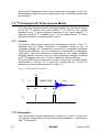
7.2.2
Pulse Sequence ........................................................................................................................ 64
7.2.3
Set the 1H Carrier Frequency................................................................................................... 64
7.2.4
Set the 13C Carrier Frequency and the Spectral Width .............................................................. 65
7.2.5
Calibration: High Power.......................................................................................................... 67
7.2.6
Calibration: Low Power for WALTZ-16 Decoupling................................................................. 67
7.3 13C DECOUPLER 90° PULSE (INVERSE MODE) ......................................................................................... 68
7.3.1
Sample..................................................................................................................................... 68
7.3.2
Preparation ............................................................................................................................. 68
7.3.3
Set the 13C Carrier Frequency.................................................................................................. 69
7.3.4
Set the 1H Carrier Frequency and the Spectral Width ............................................................... 70
7.3.5
Preparations for the Inverse Pulse Calibration......................................................................... 71
7.3.6
Calibration: High Power.......................................................................................................... 73
7.3.7
Calibration: Low Power for GARP Decoupling ........................................................................ 73
7.4 1D INVERSE TEST SEQUENCE ................................................................................................................ 74
8 ADVANCED 1D 13C EXPERIMENTS...................................................................................................... 77
8.1 13C EXPERIMENTS WITH GATED 1 H-DECOUPLING ................................................................................... 77
8.1.1
Plotting 1D 13C Spectra............................................................................................................ 79
8.2 DEPT................................................................................................................................................... 80
8.2.1
Acquisition and Processing ...................................................................................................... 81
8.2.2
Reference Spectra .................................................................................................................... 81
8.2.3
Create a New Data Set............................................................................................................. 81
8.2.4
Spectrum Acquisition ............................................................................................................... 82
8.2.5
Processing of the Spectrum ...................................................................................................... 82
8.2.6
Other spectra........................................................................................................................... 83
8.2.7
Plot the spectra........................................................................................................................ 83
9 COSY ......................................................................................................................................................... 85
9.1 INTRODUCTION ..................................................................................................................................... 85
9.2 MAGNITUDE COSY............................................................................................................................... 85
9.2.1
Pulse Sequence ........................................................................................................................ 86
9.2.2
Acquisition of the 2D COSY Spectrum ...................................................................................... 86
9.2.3
Processing of the 2D COSY Spectrum ...................................................................................... 87
9.2.4
Plotting the Spectrum............................................................................................................... 88
9.3 DOUBLE-QUANTUM FILTERED (DQF) COSY......................................................................................... 90
9.3.1
Pulse Sequence ........................................................................................................................ 90
9.3.2
Acquisition and Processing ...................................................................................................... 90
Avance 1D/2D
BRUKER
3
9.3.3
Phase correct the spectrum ...................................................................................................... 91
9.3.4
Plot the spectrum ..................................................................................................................... 92
9.4 DOUBLE-QUANTUM FILTERED COSY USING PULSED FIELD GRADIENTS (GRASP-DQF-COSY) ............. 93
9.4.1
Pulse Sequence ........................................................................................................................ 94
9.4.2
Acquisition and Processing ...................................................................................................... 94
10 TOCSY..................................................................................................................................................... 97
10.1 INTRODUCTION ................................................................................................................................... 97
10.2 ACQUISITION ...................................................................................................................................... 98
10.3 PROCESSING........................................................................................................................................ 99
10.4 PHASE CORRECTION .......................................................................................................................... 100
10.5 PLOT THE SPECTRUM ......................................................................................................................... 101
11 ROESY................................................................................................................................................... 103
11.1 INTRODUCTION ................................................................................................................................. 103
11.2 ACQUISITION .................................................................................................................................... 104
11.3 PROCESSING...................................................................................................................................... 105
11.4 PHASE CORRECTION AND PLOTTING .................................................................................................. 106
12 NOESY................................................................................................................................................... 107
12.1 INTRODUCTION ................................................................................................................................. 107
12.2 ACQUISITION AND PROCESSING ......................................................................................................... 108
12.2.1 Optimize Mixing Time............................................................................................................ 109
12.2.2 Acquire the 2D data set.......................................................................................................... 110
12.3 PROCESSING...................................................................................................................................... 110
12.4 PHASE CORRECTION AND PLOTTING .................................................................................................. 110
13 XHCORR............................................................................................................................................... 113
13.1 INTRODUCTION ................................................................................................................................. 113
13.2 ACQUISITION .................................................................................................................................... 114
13.2.1 1H Reference Spectrum............................................................................................................ 114
13.2.2 13C Reference Spectrum........................................................................................................... 114
13.2.3 Acquire the 2D Data Set ........................................................................................................ 115
13.3 PROCESSING...................................................................................................................................... 116
13.4 PLOTTING THE SPECTRUM ................................................................................................................. 117
14 COLOC.................................................................................................................................................. 119
14.1 INTRODUCTION ................................................................................................................................. 119
14.2 ACQUISITION AND PROCESSING ......................................................................................................... 120
15 HMQC.................................................................................................................................................... 123
15.1 INTRODUCTION ................................................................................................................................. 123
15.2 ACQUISITION .................................................................................................................................... 124
15.2.1 Optimize d7 (only for HMQC with BIRD)............................................................................... 126
15.2.2 Acquire the 2D data set.......................................................................................................... 126
15.3 PROCESSING...................................................................................................................................... 126
15.4 PHASE CORRECTION .......................................................................................................................... 127
15.5 PLOTTING ......................................................................................................................................... 127
16 HMBC.................................................................................................................................................... 129
16.1 INTRODUCTION ................................................................................................................................. 129
16.2 ACQUISITION AND PROCESSING ......................................................................................................... 130
17 1H,13C INVERSE SHIFT CORRELATION- EXPERIMENTS USING PFG'S ................................... 133
17.1 INTRODUCTION ................................................................................................................................. 133
17.2 GRASP-HMQC................................................................................................................................ 133
17.3 GRASP-HMBC ................................................................................................................................ 134
17.4 GRASP-HSQC................................................................................................................................. 135
17.5 ACQUISITION AND PROCESSING ......................................................................................................... 136
18 1D NOE DIFFERENCE ........................................................................................................................ 141
4
BRUKER
Avance 1D/2D
18.1 INTRODUCTION ................................................................................................................................. 141
18.2 ACQUISITION .................................................................................................................................... 142
18.2.1 Create a new file directory ..................................................................................................... 142
18.2.2 1H reference spectrum ............................................................................................................ 142
18.2.3 Select the resonances for irradiation ...................................................................................... 143
18.2.4 Set up the acquisition parameters........................................................................................... 143
18.2.5 Optimize the irradiation power and duration .......................................................................... 144
18.2.6 Perform the multiple NOE experiment .................................................................................... 145
18.3 PROCESSING...................................................................................................................................... 146
18.3.1 Perform the Phase Correction................................................................................................ 146
18.3.2 Create NOE Difference Spectra ............................................................................................. 146
18.3.3 Quantitate the NOE ............................................................................................................... 147
19 T1 MEASUREMENT............................................................................................................................. 149
19.1 INTRODUCTION ................................................................................................................................. 149
19.2 ACQUISITION .................................................................................................................................... 150
19.2.1 Write the variable delay list ................................................................................................... 150
19.2.2 Set up the acquisition parameters........................................................................................... 151
19.2.3 Acquire the 2D data set.......................................................................................................... 151
19.3 PROCESSING...................................................................................................................................... 152
19.3.1 Write the integral range file and baseline point file................................................................. 152
19.4 T1 CALCULATION .............................................................................................................................. 153
19.4.1 Check T1 curves ..................................................................................................................... 154
19.4.2 Check numerical results......................................................................................................... 154
19.4.3 T1 parameters ........................................................................................................................ 155
19.5 CREATE A STACKED PLOT ................................................................................................................. 155
20 SELECTIVE EXCITATION................................................................................................................. 159
20.1 INTRODUCTION ................................................................................................................................. 159
20.2 SELECTIVE PULSE CALIBRATION........................................................................................................ 159
20.2.1 1H reference spectrum ............................................................................................................ 160
20.2.2 Selective one-pulse sequence.................................................................................................. 160
20.2.3 Define the pulse shape ........................................................................................................... 160
20.2.4 Acquire and process the selective one-pulse spectrum............................................................. 160
20.2.5 Perform the pulse calibration................................................................................................. 162
20.3 SELECTIVE COSY ............................................................................................................................. 163
20.3.1 Acquisition ............................................................................................................................ 164
20.3.2 Processing............................................................................................................................. 165
20.4 SELECTIVE TOCSY........................................................................................................................... 166
20.4.1 Variable Delay List................................................................................................................ 167
20.4.2 Acquisition ............................................................................................................................ 167
20.4.3 Processing............................................................................................................................. 168
Avance 1D/2D
BRUKER
5
6
BRUKER
Avance 1D/2D
1 Introduction
This manual gives an introduction into basic one- and two-dimensional
nuclear magnetic resonance (NMR) spectroscopy. After a short introduction
the acquisition of basic 1D 1H and 13C NMR spectra is described in the
Chapters 4 to 8. Homonuclear 2D [1H,1H] correlation spectra are described in
Chapter 9 (COSY), 10 (TOCSY), 11 (ROESY) and 12 (NOESY).
Heteronuclear 2D [13C,1H] correlation experiments are described in Chapter
13 (XHCORR), 14 (COLOC), 15 (HMQC) and 16 (HMBC). The Chapter 17
contains the description of inverse 2D [13C,1H] correlation experiments using
pulsed field gradients, and some special NMR experiments are described in
Chapters 18 to 20.
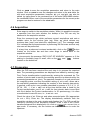
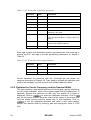
1.1 An Important Note on Power Levels
Several places throughout this manual, the user is asked to set the power
levels pl1, pl3, etc. to the “high power” level for the corresponding channel
(f1 or f2). In order to avoid damaging the probehead or other hardware
components, the user is advised to use only the power levels indicated in
Table 1 below, if no other information (e.g. final acceptance tests) is
available.
Note that these “power levels” are really attenuation levels, and so a higher
value corresponds to a lower power. Also note that these power levels
pertain only to the specific spectrometers and amplifiers listed below, which
correspond to the AVANCE instruments as of July 2000. It is assumed that
no correction tables (CORTAB) are existing.
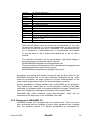
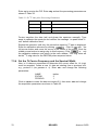
Table 1: Suggested “Proton and Carbon High Power” Levels for Avance
Instruments
Nucleus
Spectrometer
Amplifier
Power Level
Avance
BLA2BB
≥ + 3dB
BLARH100
≥ + 3dB
BLAXH300/50
≥
BLAXH20
= - 6dB
BLAXH40
= - 3dB
BLAXH100/50
≥
0dB
BLAXH150/50
≥
0dB
BLAXH300/50
≥
0dB
BLARH100
≥ + 3dB
Avance DPX
0dB
1
H
Avance DRX
Avance DMX
Avance 1D/2D
BRUKER
7
Nucleus
Spectrometer
Amplifier
Power Level
Avance
BLA2BB
≥ + 6dB
BLAX300/50
≥ + 6dB
BLAX300
≥ + 6dB
BLAX500
≥ + 9dB
BLAXH20
= - 6dB
BLAXH40
= - 6dB
BLAXH100/50
≥ - 3dB
BLAXH40
≥ - 3dB
BLAXH150/50
≥
0dB
BLAXH300/50
≥
6dB
BLAX300
≥ + 6dB
BLAX500
≥ + 9dB
Avance DPX
13
C
Avance DRX
Avance DMX
1.2 NMR Spectrometer
The NMR spectrometer consists of three major components: (1) The
superconducting magnet with the probe, which contains the sample to be
measured; (2) The console, which contains all the electronics used for
transmission and reception of radio frequency (rf) pulses through the preamplifier to the probe; (3) The computer, from where the operator runs the
experiments and processes the acquired NMR data.
8
BRUKER
Avance 1D/2D
2 Theoretical Background
2.1 Introduction
In the next few paragraphs, an attempt will be made to introduce the spin
operator as a handy tool for understanding more or less involved NMR
experiments. However, at the same time, we will try to limit the mathematical
and purely academic sides of this formalism to an absolute minimum. In other
words: you should not need a degree in mathematical science to be able to
use and understand the spin operator formalism as a tool for a better
understanding of the experiments covered during this course.
Also being strictly correct, this introduction will try to avoid as many tricky or
complicated issues as possible. The goal will be to enable the use of the spin
operator formalism as a tool and not to give an introduction to quantum
mechanics.
In order to make the first contact with the subject a bit smoother, we will
introduce the first concepts in analogy to the Bloch equations. The Bloch
equations are very intuitive and convenient to explain relatively simple 1D
experiments. But coupled 2-spin systems are already a challenge in this
model, while a 3-spin system becomes impossible to describe. The spin
operator formalism for a one-spin system is very similar to the Bloch
equations and we will use this similarity to ease the first contact. However it
should be kept in mind, that while the Bloch formalism is concerned with
macroscopic magnetization only, the spin operator formalism describes the
full state of the spin system, including non-observable terms. Those nonobservable terms however, ignored in the Bloch equations, are the basis of
most modern experiments!
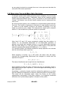
2.2 Classical Description of NMR
Among the various atomic nuclei, about a hundred isotopes possess an
intrinsic angular momentum, called spin and written hI . They also possess a
magnetic moment µ which is proportional to their angular momentum:
µ = γhI
where γ is the gyromagnetic ratio.
r
The
Larmor theorem states that the motion of a magnetic moment M (where
r
M represents the bulk magnetic moment of a collection of identical nuclei) in
a magnetic field B0 is a precession around that field. The precession
frequency is given by:
Avance 1D/2D
BRUKER
9
ω 0 = −γB0
Larmor frequency
By convention, the external static field (B0) is assumed to be along the z-axis
and the transmitter/receiver coil along either the x- or y-axis. After the sample
has reached its thermal equilibrium (in this context: the equilibrium
magnetic
r
polarization!), the system shows a magnetization vector M along the z-axis.
In this state, no NMR signal is observed, as we have no transverse rotating
magnetization.
By application of
an additional rotating magnetic field B1 in the x-y-plane,r the
r
orientation of M can be tilted into the x-y plane as the precession of M is
always around the total magnetic field, e.g. the vector sum of B0 and B1. A
rotating magnetic
field is obtained by using RF-pulses. To describe the
r
motion of M in the presence of the rotating B1, it is convenient to use a
rotating coordinate system instead of a static one. By convention, B1 is
assumed to be along the x-axis of a coordinate system rotating around the zaxis. The rotating coordinate system is chosen to rotate at the same
frequency than B1, thus making both B0 and B1 time independent in this
reference system. The Bloch equations in this coordinate system are then:
d r
M x = M yr {γB0 + ω }
dt
d r
M y = M xr {γB0 + ω } + γB1M z
dt
d
M z = − M yrγB1
dt
ω is the rotational frequency of the coordinate system. The relaxation during
the rf-pulse is neglected, as the pulse is assumed to be very short compared
with the relaxation time. By assuming an effective magnetic field:
Beff = B0 +
ω
γ
we recognize the Bloch equation from the static coordinate system. The
magnetization precessess in the rotating frame around Beff instead of B0. By
choosing ω to be:
ω = −γB0
Beff vanishes and the Bloch equation simplifies to:
d
M
dt
d
M
dt
d
M
dt
r
x
= 0
r
y
= γB1M
z
= −M
r
y
z
γB1
Assuming the magnetization at time 0 to be along the z-axis with amplitude
M0, we find the following solution to the above equation system:
10
BRUKER
Avance 1D/2D
M yr (t ) = M 0 sin(γB1t )
M z (t ) = M 0 cos(γB1t )
This means, that the magnetization vector is precessing around Beff = B1, e.g.
the magnetization is rotating around the B1 axis which is aligned with the xaxis of the reference system. If we choose the time t of suitable duration, we
obtain:
β = γB1t =
π
2
which is defined as the 90 degree pulse. As we can see, the 90° creates a
maximum of y-magnetization which in turn yields a maximal signal intensity.
This results will now be presented in the quantum mechanical notation.
2.3 Spin Operators of a One-Spin System
In the spin operator formalism, the state of a spin is represented by a linear
combination of four operators: Ix, Iy, Iz and ½ E. The first three can be
understood as Mx, My and Mz respectively, also this is not strictly correct, as
Mx refers to a macroscopic magnetization while Ix refers to a single spin. For
all practical purposes, this detail can be neglected. The fourth operator, ½ E
or unity operator, is added for reasons of mathematical consistency and is
usually omitted in the notation. We will also follow this convention and omit
½ E.
The operators form a basis in the so called Liouville space, which is the
mathematical frame work, in which the spin system is described. But we don’t
need to worry about this for the moment.
2.4 The Thermal Equilibrium State
All NMR experiments start from the thermal equilibrium. In thermal
equilibrium, the classical description gives rise to a magnetic moment parallel
to the static field. This is due to the fact, that the energy level for spins in a
parallel orientation with the external field is slightly lower than the one for the
antiparallel spins. According to Boltzman, the lower energy level will have a
higher population than the high energy level, the difference being
proportional to the energy difference. The energy difference between these
two “Zeeman levels” being very small, the resulting population difference is in
the order of 6.5*10-3%! Following the convention of the static field being
aligned with the z-axis of the reference frame, the equilibrium magnetization
is also called Mz.
In the spin operator formalism, this result has to be derived from statistical
quantum mechanics considerations using ensemble averages and population
probabilities. For us, it will be good enough to know the following result:
σ eq = I z
Avance 1D/2D
BRUKER
11
σeq is the equilibrium density matrix. The density matrix represents the state
of the spin system under investigation and is represented as a linear
combination of the basis spin operators. For a one-spin system in thermal
equilibrium, the coefficients of all but the Iz basis operator vanish. To
understand, what happens during an NMR experiment, we will have to
evaluate the changes in the density matrix during the experiment, starting
from the equilibrium matrix. These changes are also referred to as evolution
of the system.
There are two basic type of evolutions: under the effect of an external
perturbation, e.g. a RF-pulse or the unperturbed evolution which will
eventually bring the system back to the thermal equilibrium.
2.5 Effect of RF-Pulses
Let us first consider the evolution under an RF-pulse. In modern
spectrometers, pulses are only applied in the x-y- or transverse plane. Pulses
in-between the x- and y-axis are calculated by a combination of a rotation
around the z-axis followed by an x- or y-pulse.
In the classical description, we moved to a rotating coordinate system to
describe the effect of the rf-pulse. In the Spin Operator formalism, a similar
approach is taken, although with a slightly different vocabulary. The “rotating
coordinate system” is called rotating frame or interaction frame.
For the same reason then in the classical approach, the rotational axis is
chosen along the z-axis, parallel to the static field B0 and the B1 field is
assumed along the x-axis. The interaction frame rotates by definition with the
frequency of the rf-pulse (or the reference frequency of the detector, which is
identical to the former) and is called the carrier frequency. As a
consequence, all Larmor frequencies are changed into chemical shift
frequencies, defined by:
δ = ω0 − ω
The pulse is assumed to be of very short duration, such that chemical shift
evolution and relaxation during the pulse can be ignored. Then the effect of
an rf-pulse is that of a rotation along the pulse axes according to the following
calculus rules:
βx
I z →
I z cos β − I y sin β
β
y
I z →
I z cos β + I x sin β
βx
I x →
Ix
β
y
I y →
Iy
β
y
I x →
I x cos β − I z sin β
βx
I y →
I y cos β + I z sin β
If the flip angle β = 90° then:
12
BRUKER
Avance 1D/2D
y ,x

→ ± I x, y
I z 
90
y,x

→ mIz
I x, y 
90
We find the expected result, that a 90° pulse will generate transverse
magnetization. The rest of this chapter will be concerned with following the
fate of this transverse magnetization in time.
We introduced tacitly the arrow notation, where we find on the left side the
system before and on the right side after the specific evolution under the
operator noted above the arrow. This notation is simple, very convenient and
not only limited to the description of rf-pulses. We will discuss this notation in
more detail in the next section.
2.6 The Hamiltonian: Evolution of Spin Systems in Time
The arrow notation, which was introduced like a deus ex machina in the
previous section, needs some more explanation. First, let us introduce a new
type of operator, the Hamiltonian H . Each quantum mechanical system has
its associated H which describes the possible changes of energy of the
system. Once the H is known, the evolution of the density matrix of the
corresponding system can be described by:
σ (t ) = exp( −i ⋅ H ⋅ t )σ (0) exp(i ⋅ H ⋅ t )
under the condition that H by itself is time independent. The above equation
in the arrow notation will be:
Ht
σ (0) 
→ σ (t )
In other words, the arrow notation is a compact an elegant way of describing
the different steps of a time evolution under different Hamiltonians. The
Hamiltonian corresponding to an rf-pulse, neglecting relaxation and chemical
shift, is given by:
H = γ ⋅ B
1
⋅ I
x
which describes a precession around Ix with frequency γB1. The
corresponding flip angle β equals β = γ B1 t, where t is the duration of the
pulse:
H t = γ ⋅ B1 ⋅ I x ⋅ t = β ⋅ I x
This result illustrates, that for a given flip angle β, one can either use a high
B1-field or a long pulse duration t. Furthermore, the gyromagnetic ratio γ also
strongly influences the behavior of the flip angle. This explains the need for
specific rf power for different nuclei.
2.6.1 Effect of Chemical Shift Evolution
So far, we discussed the Hamiltonian corresponding to an system under
perturbation by an rf-pulse and neglecting chemical shift and relaxation at the
Avance 1D/2D
BRUKER
13
same time. In this simple introduction, relaxation will always be neglected.
The chemical shift Hamiltonian of the unperturbed system will have to
describe a precession around the static field. We have to remember, that for
convenience, all operations are done in the interaction frame, e.g. that all
Larmor frequencies are replaced by the chemical shift or precisely by the
difference between the Larmor- and the carrier frequency.
Under this condition, the chemical shift Hamiltonian is given by:
H = δ ⋅ Iz
where δ is: δ = ω 0 − ω , where ω0 is the Larmor frequency of the spin and ω
the carrier frequency of the interaction frame. In case that the Larmor
frequency is different from the carrier frequency, this is a rotation around Iz in
the rotating frame. If there is no relaxation shifting the system back to thermal
equilibrium, this is the expected result.
The calculus rules for the chemical shift evolution are the following:
⋅ I z ⋅t
I z δ
→ I z
δ ⋅I z ⋅t
I x 
→ I x cos(δ t ) + I y sin( δ t )
δ ⋅I z ⋅t
I y 
→ I y cos(δ t ) − I x sin( δ t )
The time t is the period, during which the Hamiltonian is valid. The
Hamiltonian of a spin system can change with time, for example if the
experimental setup prescribes first a rf-pulse and then a period of
unperturbed evolution. For the calculus rules given to be valid, it is
mandatory, that each Hamiltonian is time independent during the time t.
This means, that chemical shift can evolve only in the state of magnetization
within the x/y plane a.k.a. “transversal magnetization”.
Thus, the whole experiment is divided into time intervals, during which the
Hamiltonian can be made time independent by choice of a suitable
interaction frame. Typical experiments are divided in pulse intervals and free
evolution times.
During the pulses, the chemical shift and scalar coupling interaction is
ignored. Only the applied B1 field is considered. This approach is justified for
pulses with tPulse<<T1,T2.
The question now is how to interpret this quantum mechanical result in terms
of macroscopic measurements. To answer this question, we will need to
discuss the difference between operators and physical observables. This will
be the subject of the next paragraph.
2.7 Observable Signals and Observable Operators
Not all operators correspond to physical forces or fields. In fact, only a
minority gives rise to detectable energy changes of any kind. In our particular
case, only Ix, Iy and Iz are physical observables, e.g. they correspond to
physical phenomena, which can be measured. In a one spin system,
obviously only ½ E is not a physical observable (we neglected this operator
14
BRUKER
Avance 1D/2D
already in the beginning). But as we will see in paragraph 2.8.1, a two spin
system exhibits 16 operators but only 6 of them are physically observable.
So what are the “unobservable” operators good for?
•
First, they describe quantum mechanical interactions in the system and
•
second, they can evolve into observable magnetization!
A typical example for this is the scalar coupling, which is described in
paragraph 2.8.1.
How is the FID obtained from these physical observables? The trick is to
introduce another operator with the same qualities as the physical detector.
In the spectrometer, quadrature detection is used, that is we observe the
magnetic flux along the x- and along the y-axis in the rotating frame and
combine the results into one complex valued number. The corresponding
operators are:
I+ = I x + i ⋅ I y
I− = Ix − i ⋅ I y
In principle, we have the choice of selecting either I+ or I-, depending how we
combine the physical measurements. By convention, I+ is used as the
detection operator. It should be noted, that I+ as the detector selects the Icomponent of the signal. To calculate the physical value of an operator at a
given time, the trace of this operator is multiplied by the relevant density
operator:
I + (t ) = Tr{I + ⋅ σ (t )}
It is convenient to express σ in terms of the operators I+ and I- to evaluate this
expression. Let’s continue with the example of the one spin system: during
detection (t2), we get the following expression for our density operator:
σ (t2 ) = I x cos(δ ⋅ t2 ) + I y sin(δ ⋅ t2 )
After rewriting the equation for I+ and I-:
1
(I + + I − )
2
i
I y = − (I + − I − )
2
Ix =
we can substitute Ix and Iy in:
σ (t2 ) = I x cos(δ ⋅ t 2 ) + I y sin(δ ⋅ t 2 )
1
(I + + I − ) ⋅ cos(δ ⋅ t 2 ) + ( − i )(I + − I − ) ⋅ sin(δ ⋅ t 2 )
2
2
1
1
= I + [cos( δ ⋅ t2 ) − i ⋅ sin(δ ⋅ t 2 )] + I − [cos( δ ⋅ t 2 ) + i ⋅ sin(δ ⋅ t2 )]
2
2
1
= I + ⋅ e − i ⋅δ ⋅t 2 + I − ⋅ e i ⋅δ ⋅t 2
2
=
(
)
When calculating the expectation value of I+ (the observable signal, we find:
Avance 1D/2D
BRUKER
15
I + (t 2 ) = Tr{I + ⋅ σ (t 2 )}
(
)
1
I + ⋅ e −i⋅δ ⋅t 2 + I − ⋅ e i⋅δ ⋅t 2 }
2
1
1
= ⋅ e −i⋅δ ⋅t2 ⋅ Tr{I + I + }+ ⋅ e i⋅δ ⋅t 2 ⋅ Tr{I + I − }
2
2
=0
= I0
1
= ⋅ I 0 ⋅ e i⋅δ ⋅t2
2
= Tr{I + ⋅
The signal function is an oscillation with the frequency δ and the amplitude
½ I0. The amplitude ½ I0 is in fact an elegant way to hide a bunch of quantum
mechanical constants and it is ignored most of the time. Normally one is
interested in relative signal intensities rather than in absolute values.
One might object, that δ is not the Larmor frequency, which one might have
expected, but only the chemical shift relative to the rotation frequency (carrier
frequency) of the interaction frame. Remember, that also the detection
operator is defined in the rotating frame, e.g. is also rotating with the carrier
frequency.
The technical realization of this “rotating detector” is achieved by mixing the
signal from the probe - which is in the MHz range - with the carrier frequency,
which is also in the MHz range. The mixing process yields the difference
frequency between the two oscillations and is of the order of few 10 kHz. The
mixing process can be understood as comparing the signal at any time with a
rotating reference vector, which is exactly what we have done in the
interaction frame with a fixed detector on the x- or y- axis.
For all practical purposes, ½ I0 is assumed to be one. and the signal function
is assumed to:
F (t 2 ) = ei ⋅δ ⋅t 2
= ei ⋅ 2⋅π ⋅ν ′⋅t 2
The radial frequency δ in radians was replaced by the frequency ν’ in Hz.
This is the unit in which the spectra are expressed finally.
The time domain function F(t2), needs to be Fourier transformed to obtain the
spectral function S(ν).
FT
F (t2 ) = ei ⋅2⋅π ⋅ν ′⋅t 2 →
S (ν ) = δ Dirac (ν − v′)
The function S(ν) is zero except for the point ν=ν’, where it is infinite. This is a
so called stick spectrum, as the intensities are meaningless and only the
frequency information is relevant. The signal function ei⋅ 2⋅π ⋅ν ⋅t 2 will come up
frequently during NMR calculations, so that it is worthwhile to remember its
Fourier transformation. Note that, while the time domain function is complex
valued, the frequency domain function is strictly real.
Things get more complex once relaxation is taken into account. To obtain
correct line shape information, relaxation becomes vitally important.
At this point, we have successfully evaluated the outcome of a simple NMR
experiment consisting of a 90º excitation pulse followed by the detection
period and the evaluation of the detection operator I+. In the next paragraph,
16
BRUKER
Avance 1D/2D
we are going to extend our example from one to two spins and calculate the
outcome of the same experiment.
2.8 Observing Two and More Spin Systems
A one-spin system does indeed not show much complexity. So let us then
proceed to a two-spin system. Traditionally there are two notations widely
used to distinguish different spins: I1 and I2 as indices or I and S with different
“names”. For protons, we use the indices notation and for heteronuclei we
use S or S1.
As a first two-spin system, let us consider at a homonuclear system with two
1
H nuclei. The number of operators in the basis of a spin system is given by
4N, where N is the number of spins in the system. Fortunately, it is very
simple to construct such a basis. The basis for two single spins (compare
section 2.3) are multiplied to yield the needed 16 operators:

1
 2 E1, 2 , I1z , I 2 z , 2 I1z I 2 z , 
1  
1   I , I , 2 I I , 2 I I , 

1y
1x 2 z
1y 2 z
I
I
I
E
⊗
I
I
I
,
,
,
,
,
,

 2 x 2 y 2 z E2  ⇒  1 x
 1x 1 y 1z
1
2  
2  

I 2 x , I 2 y , 2 I1 z I 2 x , 2 I1 z I 2 y , 


2 I1x I 2 x ,2 I1 y I 2 y , 2 I1x I 2 y , 2 I1 y I 2 x 
Note, that ½ E1 and ½ E2 were consistently omitted from the notation. In
section 2.7, we discussed observable vs. non-observable operators. In
general, only single spin operators along x, y or z are observable operators
and only those along x or y will give rise to a NMR signal. In this particular
case the operators that relevant for NMR are I1x, I2x, I1y and I2y.
In a two-spin system, the thermal equilibrium density operator now includes
also the second spin and is given by:
σ eq = I1z + I 2 z
When applying a rf-pulse, e.g. a 90º pulse, the same rules still apply.
However the corresponding Hamiltonian has changed to include also the
operator from spin 2:
H = γ ⋅ B1 ⋅ ( I1x + I 2 x )
The above Hamiltonian can be split into two Hamiltonians
H = γ ⋅ B1 ⋅ ( I1x ) and H = γ ⋅ B1 ⋅ ( I 2 x )
being applied one after the other. The first acts only on operators of spin 1
and is ignored by all spin 2 operators. The second applies accordingly only to
spin 2 operators.
Accordingly, a selective rf-pulse could be realized by applying e.g. a pulse
with the respective Hamiltonian to achieve a selective pulse on a certain spin.
This issue will be discussed again, when the theory of the inverse
experiments is discussed. In the arrow notation, if not explicitly mentioned
otherwise, the rf-pulse always applies to all spins in the system.
Avance 1D/2D
BRUKER
17
In our example, we apply a 90º pulse to the equilibrium density matrix:
y
σ eq →
σ (0) = I1x + I 2 x
90
The next step will be to evaluate the free evolution during the acquisition
time. But before we can do so, we need to have a look at the corresponding
Hamiltonian and there we will find a new phenomenon: the scalar coupling!
2.8.1 Effect of Scalar Coupling
Apart from the chemical shift, there is a second very import interaction
between spins, the scalar coupling. The scalar depends on the mediation of
electrons, which are confined in orbitals around both nuclei. The scalar
coupling is expressed in Hz and noted as J. The operator expression for the
scalar coupling is:
2π J 12 I 1z I 2 z
The above Hamiltonian expresses the scalar coupling between spin 1 and
spin 2 with a coupling constant J12. The evolution Hamiltonian for this spin
system is then:
H = δ 1 I 1z + δ 2 I 2 z + 2π J 12 I 1z I 2 z
To calculate the effect of this Hamiltonian, it is divided into 3 parts:
δ 1 I 1z
δ 2 I 2z
2π J 12 I 1z I 2 z
which are applied in sequence, where this sequence is arbitrary. After a 90°
pulse has been applied to the two spins, we first calculate the two chemical
shift terms:
1 ⋅ I1 z ⋅t
→ I 1x cos(δ 1 t ) + I 1 y sin(δ 1 t ) + I 2 z
σ eq = I 1x + I 2 x δ
2 ⋅ I 2 z ⋅t
δ
→ I 1x cos(δ 1 t ) + I 1 y sin(δ 1 t )
+ I 2 x cos(δ 2 t ) + I 2 y sin(δ 2 t ) ⇒ σ 1
The next step will be to calculate the evolution under the scalar coupling.
2.8.2 Evolution under Weak Coupling
To apply the last part of the Hamiltonian, we need some new calculus rules.
The scalar coupling term can be evaluated with a simple set of rules:
2π J 12 I1 z I 2 z t
I 1z 
 → I 1z
2π J 12 I1 z I 2 z t
I 1x 
 → I 1x cos(πJ 12 t ) + 2 I 1 y I 2 z sin(πJ 12 t )
2π J 12 I1 z I 2 z t
I 1 y 
 → I 1 y cos(πJ 12 t ) − 2 I 1x I 2 z sin(πJ 12 t )
2π J 12 I1 z I 2 z t
2 ⋅ I 1x I 2 z 
 → 2 I1x I 2 z cos(πJ 12 t ) + I 1 y sin(πJ 12 t )
2π J 12 I1 z I 2 z t
 → 2 I1 y I 2 z cos(πJ 12 t ) − I 1x sin(πJ 12 t )
2 ⋅ I 1 y I 2 z 
2π J 12 I1 z I 2 z t
 → 2 I1x I 2 y
2 ⋅ I1x I 2 y 
18
BRUKER
Avance 1D/2D
From the above equation, we immediately recognize a very important fact:
the scalar coupling can generate observable operators from non-observable
ones through free evolution! This is the reason, why we can not neglect the
non-observable operators until we apply the detection operator (signal
acquisition)!
Befitted with the above equations, we can now evaluate the last part of the
Hamiltonian:
2π J 12 I1 z I 2 z t
σ 1 
 → {I 1x cos(πJ 12 t ) + 2 I 1 y I 2 z sin(πJ 12 t )} ⋅ cos(δ 1t )
+ {I 1 y cos(πJ 12 t ) − 2 I 1x I 2 z sin(πJ 12 t )} ⋅ sin( δ 1t )
+ {I 2 x cos(πJ 12 t ) + 2 I 1z I 2 y sin(πJ 12 t )} ⋅ cos(δ 2 t )
+ {I 2 y cos(πJ 12 t ) − 2 I 1z I 2 x sin(πJ 12 t )} ⋅ sin(δ 2 t )
= σ2
after some rearrangement, this leads to:
σ 2 = I1x cos(π ⋅ J12 ⋅ t ) ⋅ cos(δ1 ⋅ t ) + I1 y cos(π ⋅ J12 ⋅ t ) ⋅ sin(δ1 ⋅ t )
+ I 2 x cos(π ⋅ J12 ⋅ t ) ⋅ cos(δ 2 ⋅ t ) + I 2 y cos(π ⋅ J12 ⋅ t ) ⋅ sin(δ 2 ⋅ t )
+ 2 ⋅ I1 y I 2 z sin(π ⋅ J12 ⋅ t ) ⋅ cos(δ1 ⋅ t ) − 2 ⋅ I1x I 2 z sin(π ⋅ J12 ⋅ t ) ⋅ sin(δ1 ⋅ t )
+ 2 ⋅ I1z I 2 y sin(π ⋅ J12 ⋅ t ) ⋅ cos(δ 2 ⋅ t ) − 2 ⋅ I1z I 2 x sin(π ⋅ J12 ⋅ t ) ⋅ sin( δ 2 ⋅ t )
= ( I1x cos(δ1 ⋅ t ) + I1 y sin( δ1 ⋅ t )) ⋅ cos(π ⋅ J12 ⋅ t )
+ ( I 2 x cos(δ 2 ⋅ t ) + I 2 y sin( δ 2 ⋅ t )) ⋅ cos(π ⋅ J12 ⋅ t )
+ (2 ⋅ I1 y I 2 z cos(δ1 ⋅ t ) − 2 ⋅ I1x I 2 z sin(δ1 ⋅ t )) ⋅ sin(π ⋅ J12 ⋅ t )
+ (2 ⋅ I1z I 2 y cos(δ 2 ⋅ t ) − 2 ⋅ I1z I 2 x sin( δ 2 ⋅ t )) ⋅ sin(π ⋅ J12 ⋅ t )
Again, the final step is the calculation of the expectation value of the
detection operator. Of course, the detection operator also needs to include
spin 2. We introduce a detection operator F+:
F+ = I1+ + I 2 +
or more general for a N spin system:
N
F+ = ∑ Ii +
i
In the previous section, we were rewriting the density operator in terms of I+
and I- to calculate the detection results. While this is very elegant, it is also
very tedious. We know from those equations that F+ is going to select F- in
the density operator and we know also, that the coefficient of F- is obtained
by using the coefficients of Fx=ΣIix minus Fy=ΣIiy times the complex constant.
Furthermore, we elegantly disposed of the ½I0 factors in a constant, which
here we can replaced by F0 or simply be omitted altogether. While neither
being elegant nor exactly correct, we can obtain very useful results much
faster then going through all the details.
Avance 1D/2D
BRUKER
19
2.8.3 The Signal Function of a Coupled Spectrum
By omitting F0, we obtain the following signal function for our coupled twospin system:
Tr{F+ ⋅ σ 2} = (cos(δ1 ⋅ t ) + i ⋅ sin( δ1 ⋅ t )) ⋅ cos(π ⋅ J12 ⋅ t )
+ (cos(δ 2 ⋅ t ) + i ⋅ sin(δ 2 ⋅ t )) ⋅ cos(π ⋅ J12 ⋅ t )
= cos(π ⋅ J12 ⋅ t ) ⋅ ei ⋅δ 1 ⋅t + cos(π ⋅ J12 ⋅ t ) ⋅ ei ⋅δ 2 ⋅t
1 i ⋅π ⋅ J12 ⋅t
1
(e
=
+ e − i⋅π ⋅ J12 ⋅t ) ⋅ ei ⋅δ 1 ⋅t + (ei ⋅π ⋅ J 12 ⋅t + e −i ⋅π ⋅ J12 ⋅t ) ⋅ ei ⋅δ 2 ⋅t
2
2
J 12
J 12
J
J
2⋅π ⋅i ⋅(ν 1 −
)⋅ t
2⋅π ⋅i ⋅(ν 2 + 12 ) ⋅t
2⋅π ⋅i ⋅(ν 2 − 12 ) ⋅t
1 2⋅π ⋅i ⋅(ν 1 + 2 )⋅t
2
2
2
(e
)
=
+e
+e
+e
2
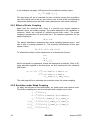
To get the results above, we made extensive use of the Euler relation. The
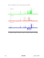
form of the signal function should look familiar: it describes a frequency
spectrum with four signals at the frequencies ν1+J12/2, ν1-J12/2, ν2+J12/2 and
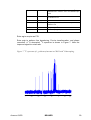
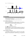
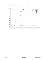
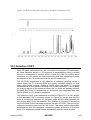
ν2-J12/2. We recognize a spectrum with two doublet signals, each doublet
having two lines of equal intensity that are separated by J12 Hz.
At this point, we are able two handle a two-spin system in a 1D experiment.
Most of the calculations using the spin operator formalism will never include
a spin system larger then two, as the number of operators quickly become
too cumbersome to handle. Nevertheless, let us take a look at a simple 3spin system in order to introduce some important simplification schemes for
handling such large system.
2.9 Simplification Schemes on A Thr e e-Spin System
Our spin system shall include three spins of the same type, all three being
coupled with each other and two coupling constants should be identical:
H = δ1I1z + δ 2 I 2 z + δ 3 I 3 z + 2 ⋅ π ⋅ J12 ⋅ I1z I 2 z + 2 ⋅ π ⋅ J13 ⋅ I1z I 3 z + 2 ⋅ π ⋅ J 23 ⋅ I 2 z I3 z
with J12=J13=J.
The full set of spin operators includes 43=64 elements and we certainly don’t
want to mess with that many operators! The first simplification consists in
only considering one spin, e.g. instead of using the full equilibrium density
matrix we use only a reduced form. In this way, we will obtain the signal
originating from that particular spin only. Most of the time, this is absolutely
sufficient. In our example, we will look at spin 1 only.
σ eq = I1z y → σ 0 = I1x
90
Again, the Hamiltonian is split it into chemical shift terms and scalar coupling
terms which are the applied subsequently. But this time, we will only keep the
terms including I1{x,y,z}, knowing that the other terms will not have any effect
on σ0:
20
BRUKER
Avance 1D/2D
δ1I1z
2 ⋅ π ⋅ J12 ⋅ I1z I 2 z
2 ⋅ π ⋅ J13 ⋅ I1z I 3 z
Applying this reduced Hamiltonian to σ0 yields:
H ⋅t
σ 0 →
I1x cos(π ⋅ J13 ⋅ t ) ⋅ cos(π ⋅ J12 ⋅ t ) ⋅ cos(δ1 ⋅ t )
+
I1 y cos(π ⋅ J13 ⋅ t ) ⋅ cos(π ⋅ J12 ⋅ t ) ⋅ sin(δ1 ⋅ t )
+ 2 I1 y I 3 z sin(π ⋅ J13 ⋅ t ) ⋅ cos(π ⋅ J12 ⋅ t ) ⋅ cos(δ1 ⋅ t )
− 2 I1x I 3 z sin(π ⋅ J13 ⋅ t ) ⋅ cos(π ⋅ J12 ⋅ t ) ⋅ sin(δ1 ⋅ t )
+ 2 I1 y I 2 z cos(π ⋅ J13 ⋅ t ) ⋅ sin(π ⋅ J12 ⋅ t ) ⋅ cos(δ1 ⋅ t )
− 2 I1x I 2 z cos(π ⋅ J13 ⋅ t ) ⋅ sin(π ⋅ J12 ⋅ t ) ⋅ sin(δ1 ⋅ t )
− 4 I1x I 2 z I3 z sin(π ⋅ J13 ⋅ t ) ⋅ sin(π ⋅ J12 ⋅ t ) ⋅ cos(δ1 ⋅ t )
− 4 I1 y I 2 z I3 z sin(π ⋅ J13 ⋅ t ) ⋅ sin(π ⋅ J12 ⋅ t ) ⋅ sin( δ1 ⋅ t )
= σ1
The corresponding signal function is:
Tr{I1+ ⋅ σ 1} = cos(π ⋅ J13 ⋅ t ) ⋅ cos(π ⋅ J12 ⋅ t ) ⋅ cos(δ1 ⋅ t )
+ i ⋅ cos(π ⋅ J13 ⋅ t ) ⋅ cos(π ⋅ J12 ⋅ t ) ⋅ sin(δ1 ⋅ t )
=
1 2⋅π ⋅i⋅(ν 1 +
(e
4
J 13 J 12
+
) ⋅t
2
2
2⋅π ⋅i ⋅(ν 1 +
J 13 J 12
−
) ⋅t
2
2
+e
+e
+e
2⋅π ⋅i ⋅(ν 1 −
2 ⋅π ⋅i ⋅(ν 1 −
J 13 J 12
+
) ⋅t
2
2
J 13 J 12
−
)⋅ t
2
2
)
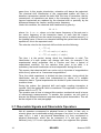
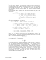
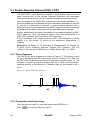
In the case, where J12=J13=J, this simplifies to:
Tr{I1+ ⋅ σ 1} =
1 2⋅π ⋅i ⋅(ν 1 + J )⋅t
(e
+ 2 ⋅ e 2⋅π ⋅i ⋅ν 1 ⋅t + e 2⋅π ⋅i ⋅(ν 1 − J )⋅t )
4
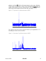
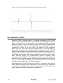
which is the well known 1:2:1 triplet we expected! Note, that the J23 is totally
irrelevant for the signal of the spin 1.
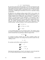
We have now seen 3 examples of a 1D-experiment. Let us now turn to 2Dexperiments. As an example for all 2D-experiments, we will study the most
fundamental 2D, the magnitude COSY experiment.
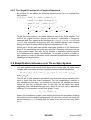
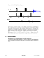
2.10 The COSY Experiment
The minimum spin system size for a COSY is a two spin system, as we need
at least two coupled spins. The pulse sequence of a COSY is very simple:
first, we use a 90º excitation pulse from the y-direction, followed by a free
evolution time t1 and a second 90º pulse around y just before the acquisition
time t2. As you may have noticed, the number of operator terms has a
tendency to dramatically increase during free evolution periods. Therefore we
will discuss more simplifications in order to keep the problem within
reasonable size.
For the COSY, we use a two-spin system with the Hamiltonian:
Avance 1D/2D
BRUKER
21
H = δ 1 ⋅ I1z + δ 2 ⋅ I 2 z + 2 ⋅ π ⋅ J12 ⋅ I1z I 2 z
For the equilibrium density operator, again we use the reduced version from
the previous section:
σ eq = I1z y → σ 0 = I1x
90
The evolution of σ0 under the above Hamiltonian therefore yields:
H ⋅t1
σ 0 
→ {I1x cos(π ⋅ J12 ⋅ t1 ) + 2 ⋅ I1 y I 2 z sin(π ⋅ J12 ⋅ t1 )} ⋅ cos(δ1 ⋅ t1 )
+ {I1 y cos(π ⋅ J12 ⋅ t1 ) − 2 ⋅ I1x I 2 z sin(π ⋅ J12 ⋅ t1 )} ⋅ sin(δ1 ⋅ t1 )
= I1x cos(π ⋅ J12 ⋅ t1 ) ⋅ cos(δ1 ⋅ t1 )
+ I1 y cos(π ⋅ J12 ⋅ t1 ) ⋅ sin(δ1 ⋅ t1 )
+ 2 ⋅ I1 y I 2 z sin(π ⋅ J12 ⋅ t1 ) ⋅ cos(δ1 ⋅ t1 )
− 2 ⋅ I1x I 2 z sin(π ⋅ J12 ⋅ t1 ) ⋅ sin(δ1 ⋅ t1 ) ⇒ σ 1
The first evolution period is identical to what we know from the 1D-example.
The 2D-experiment starts now by applying a second pulse after the first
evolution period during t1:
y
− I1z cos(π ⋅ J12 ⋅ t1 ) ⋅ cos(δ1 ⋅ t1 )
σ 1 →
90
+ I1 y cos(π ⋅ J12 ⋅ t1 ) ⋅ sin(δ1 ⋅ t1 )
+ 2 ⋅ I1 y I 2 x sin(π ⋅ J12 ⋅ t1 ) ⋅ cos(δ1 ⋅ t1 )
+ 2 ⋅ I1z I 2 x sin(π ⋅ J12 ⋅ t1 ) ⋅ sin(δ1 ⋅ t1 ) ⇒ σ 2
We now could simply apply the Hamiltonian again for the evolution during t2
and battle through 16 operators with countless coefficients just to realize, that
in fact very few of the original operators contribute to the observable
magnetization. It’s probably more rewarding however, to consider σ2 for a
while and try to figure out, which operators will evolve into observable
magnetization and which will just keep us busy.
I1z is a clear cut case, as we can see from our calculus table: it will not evolve
at all. The same is true for I1yI2x. The reduced density matrix relevant for the
observable magnetization σ2’ is then:
σ ′2 = I1 y cos(π ⋅ J12 ⋅ t1 ) ⋅ sin(δ1 ⋅ t1 )
+ 2 ⋅ I1z I 2 x sin(π ⋅ J12 ⋅ t1 ) ⋅ sin(δ1 ⋅ t1 )
Applying the chemical shift part of the Hamiltonian yields:
δ 1 ⋅ I1z + δ 2 ⋅ I 2 z ) t 2
σ 2′ (
  → [ I1 y cos(δ1 ⋅ t2 ) − I1x sin( δ1 ⋅ t2 )] cos(π ⋅ J12 ⋅ t1 ) ⋅ sin(δ1 ⋅ t1 )
+ 2 ⋅ I1z [ I 2 x cos(δ 2 ⋅ t2 ) + I 2 y sin(δ 2 ⋅ t2 )]sin(π ⋅ J12 ⋅ t1 ) ⋅ sin( δ1 ⋅ t1 )
= − I1x sin(δ 1 ⋅ t2 ) ⋅ cos(π ⋅ J12 ⋅ t1 ) ⋅ sin(δ1 ⋅ t1 )
+ I1 y cos(δ1 ⋅ t2 ) ⋅ cos(π ⋅ J12 ⋅ t1 ) ⋅ sin(δ1 ⋅ t1 )
+ 2 ⋅ I1z I 2 x cos(δ 2 ⋅ t2 ) ⋅ sin(π ⋅ J12 ⋅ t1 ) ⋅ sin(δ 1 ⋅ t1 )
+ 2 ⋅ I1z I 2 y sin(δ 2 ⋅ t2 ) ⋅ sin(π ⋅ J12 ⋅ t1 ) ⋅ sin( δ1 ⋅ t1 ) ⇒ σ 3
Finally, the coupling Hamiltonian is applied:
22
BRUKER
Avance 1D/2D
σ3
2⋅π ⋅ J12 ⋅I1 z I 2 z ⋅t 2

 → σ 4
σ 4 = − (I1x cos(π ⋅ J 12 ⋅ t 2 ) + 2 ⋅ I1 y I 2 z sin(π ⋅ J 12 ⋅ t 2 ) )sin(δ 1 ⋅ t 2 ) ⋅ cos(π ⋅ J 12 ⋅ t1 ) ⋅ sin( δ 1 ⋅ t1 )
+ (I1 y cos(π ⋅ J 12 ⋅ t 2 ) − 2 ⋅ I1x I 2 z sin(π ⋅ J 12 ⋅ t 2 ))cos(δ 1 ⋅ t 2 ) ⋅ cos(π ⋅ J 12 ⋅ t1 ) ⋅ sin(δ 1 ⋅ t1 )
+ (2 ⋅ I1z I 2 x cos(π ⋅ J 12 ⋅ t 2 ) + I 2 y sin(π ⋅ J 12 ⋅ t 2 ) )cos(δ 2 ⋅ t 2 ) ⋅ sin(π ⋅ J 12 ⋅ t1 ) ⋅ sin( δ 1 ⋅ t1 )
+ (2 ⋅ I1z I 2 y cos(π ⋅ J 12 ⋅ t 2 ) − I 2 x sin(π ⋅ J 12 ⋅ t 2 ) )sin(δ 2 ⋅ t 2 ) ⋅ sin(π ⋅ J 12 ⋅ t1 ) ⋅ sin(δ 1 ⋅ t1 )
= − I1x cos(π ⋅ J 12 ⋅ t 2 ) ⋅ sin( δ 1 ⋅ t 2 ) ⋅ cos(π ⋅ J 12 ⋅ t1 ) ⋅ sin(δ 1 ⋅ t1 )
+ I1 y cos(π ⋅ J 12 ⋅ t 2 ) ⋅ cos(δ 1 ⋅ t 2 ) ⋅ cos(π ⋅ J 12 ⋅ t1 ) ⋅ sin( δ 1 ⋅ t1 )
− I 2 x sin(π ⋅ J 12 ⋅ t 2 ) ⋅ sin( δ 2 ⋅ t 2 ) ⋅ sin(π ⋅ J 12 ⋅ t1 ) ⋅ sin( δ 1 ⋅ t1 )
+ I 2 y sin(π ⋅ J 12 ⋅ t 2 ) ⋅ cos(δ 2 ⋅ t 2 ) ⋅ sin(π ⋅ J 12 ⋅ t1 ) ⋅ sin(δ 1 ⋅ t1 )
− 2 ⋅ I1x I 2 z sin(π ⋅ J 12 ⋅ t 2 ) ⋅ cos(δ 1 ⋅ t 2 ) ⋅ cos(π ⋅ J 12 ⋅ t1 ) ⋅ sin(δ 1 ⋅ t1 )
− 2 ⋅ I1 y I 2 z sin(π ⋅ J 12 ⋅ t 2 ) ⋅ sin(δ 1 ⋅ t 2 ) ⋅ cos(π ⋅ J 12 ⋅ t1 ) ⋅ sin(δ 1 ⋅ t1 )
+ 2 ⋅ I1z I 2 x cos(π ⋅ J 12 ⋅ t 2 ) ⋅ cos(δ 2 ⋅ t 2 ) ⋅ sin(π ⋅ J 12 ⋅ t1 ) ⋅ sin(δ 1 ⋅ t1 )
+ 2 ⋅ I1z I 2 y cos(π ⋅ J 12 ⋅ t 2 ) ⋅ sin( δ 2 ⋅ t 2 ) ⋅ sin(π ⋅ J 12 ⋅ t1 ) ⋅ sin( δ 1 ⋅ t1 )
The corresponding signal function therefore is:
Tr{F+ ⋅ σ 4 } = − cos(π ⋅ J12 ⋅ t 2 ) ⋅ sin( δ1 ⋅ t 2 ) ⋅ cos(π ⋅ J 12 ⋅ t1 ) ⋅ sin(δ 1 ⋅ t1 )
+ i ⋅ cos(π ⋅ J12 ⋅ t 2 ) ⋅ cos(δ 1 ⋅ t 2 ) ⋅ cos(π ⋅ J 12 ⋅ t1 ) ⋅ sin(δ 1 ⋅ t1 )
− sin(π ⋅ J12 ⋅ t 2 ) ⋅ sin(δ 2 ⋅ t 2 ) ⋅ sin(π ⋅ J12 ⋅ t1 ) ⋅ sin(δ1 ⋅ t1 )
+ i ⋅ sin(π ⋅ J 12 ⋅ t2 ) ⋅ cos(δ 2 ⋅ t2 ) ⋅ sin(π ⋅ J 12 ⋅ t1 ) ⋅ sin(δ 1 ⋅ t1 )
J
J
2⋅π ⋅i⋅(ν1 + 12 )⋅t 2
2⋅π ⋅i⋅(ν1 − 12 )⋅t 2
i
2
2
⋅ cos(π ⋅ J 12 ⋅ t1 ) ⋅ sin( δ1 ⋅ t1 ) ⋅ (e
+e
)
2
J
J
2⋅π ⋅i⋅(ν 2 + 12 )⋅t2
2⋅π ⋅i⋅(ν 2 − 12 )⋅t 2
i
2
2
+ ⋅ sin(π ⋅ J12 ⋅ t1 ) ⋅ sin(δ1 ⋅ t1 ) ⋅ (e
−e
)
2
J
J
2⋅π ⋅i⋅(ν1 + 12 )⋅t 2
2⋅π ⋅i⋅(ν1 − 12 )⋅t2
1
2⋅π ⋅i⋅ν1⋅t 1
− 2⋅π ⋅i ⋅ν1⋅t1
2
2
=
⋅ cos(π ⋅ J 12 ⋅ t1 ) ⋅ (e
−e
+e
) ⋅ (e
)
4
J
J
2⋅π ⋅i ⋅(ν 2 + 12 )⋅t 2
2⋅π ⋅i⋅(ν 2 − 12 )⋅t 2
1
2
2
+ ⋅ sin(π ⋅ J12 ⋅ t1 ) ⋅ (e 2⋅π ⋅i⋅ν1⋅t1 − e −2⋅π ⋅i⋅ν1⋅t1 ) ⋅ (e
+e
)
4
J
J
J
J
2⋅π ⋅i⋅( −ν1 − 12 )⋅t1
1 2⋅π ⋅i⋅(ν1 + 212 )⋅t1 2⋅π ⋅i⋅(ν1 − 212 )⋅t1 2⋅π ⋅i⋅( −ν1 + 212 )⋅t1
2
=
⋅ (e
+e
−e
−e
)
8
=
⋅ (e
i
− ⋅ (e
8
⋅ (e
2⋅π ⋅i⋅(ν1 +
J12
)⋅t2
2
J
2⋅π ⋅i⋅(ν1 + 12 )⋅t 1
2
2⋅π ⋅i⋅(ν 2 +
J12
)⋅t2
2
+e
−e
2⋅π ⋅i ⋅(ν1 −
J12
)⋅t2
2
J
2⋅π ⋅i⋅(ν1 − 12 )⋅t 1
2
−e
2⋅π ⋅i ⋅(ν 2 −
J12
)⋅t 2
2
)
−e
2⋅π ⋅i⋅( −ν1 +
J12
)⋅t1
2
+e
2⋅π ⋅i⋅( −ν1 −
J12
)⋅t1
2
)
)
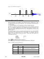
This signal function is not quiet what we expected: first the signals are
mirrored in the t1t dimension, and second the cross peak is in the imaginary
part of the spectrum. What is the problem?
To be able to distinguish between positive and negative signals, we need
both the sine and the cosine modulation. This is true for the t2 domain in the
Avance 1D/2D
BRUKER
23
above signal function, but not for the t1 part, where we only have the sine
modulation of the chemical shift. What can be done?
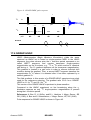
In case of the two pulse COSY, fortunately this is quite simple: we repeat the
experiment but apply the second pulse now around the x-axis instead of the
y-axis. After a lot of painstaking manipulations, we finally find for the
sequence 90y-t1-90x-t2:
σ4′ = I1x cos(π ⋅ J12 ⋅t2 )⋅cos(δ1 ⋅t2)⋅cos(π ⋅ J12 ⋅t1)⋅cos(δ1 ⋅t1)
+ I1y cos(π ⋅ J12 ⋅t2 )⋅sin(δ1 ⋅t2 )⋅cos(π ⋅ J12 ⋅t1)⋅cos(δ1 ⋅t1)
+ I2x sin(π ⋅ J12 ⋅t2)⋅cos(δ2 ⋅t2 )⋅sin(π ⋅ J12 ⋅t1)⋅cos(δ1 ⋅t1)
+ I2y sin(π ⋅ J12 ⋅t2)⋅sin(δ2 ⋅t2)⋅sin(π ⋅ J12 ⋅t1)⋅cos(δ1 ⋅t1)
+L
compared with the sequence 90y-t1-90y-t2:
σ4 = −I1x cos(π ⋅ J12 ⋅t2)⋅sin(δ1 ⋅t2)⋅cos(π ⋅ J12 ⋅t1)⋅sin(δ1 ⋅t1)
+ I1y cos(π ⋅ J12 ⋅t2)⋅cos(δ1 ⋅t2 )⋅ cos(π ⋅ J12 ⋅t1)⋅sin(δ1 ⋅t1)
− I2x sin(π ⋅ J12 ⋅t2)⋅sin(δ2 ⋅t2)⋅sin(π ⋅ J12 ⋅t1)⋅sin(δ1 ⋅t1)
+ I2y sin(π ⋅ J12 ⋅t2 )⋅cos(δ2 ⋅t2 )⋅sin(π ⋅ J12 ⋅t1)⋅sin(δ1 ⋅t1)
+L
If we sum up the signal functions of both experiments, we find:
Tr{F+ ⋅ σ 4 } + Tr{F+ ⋅ σ 4′ } = − cos(π ⋅ J 12 ⋅ t 2 ) ⋅ sin(δ 1 ⋅ t 2 ) ⋅ cos(π ⋅ J 12 ⋅ t1 ) ⋅ sin( δ 1 ⋅ t1 )
+ i ⋅ cos(π ⋅ J 12 ⋅ t 2 ) ⋅ cos(δ 1 ⋅ t 2 ) ⋅ cos(π ⋅ J 12 ⋅ t1 ) ⋅ sin( δ 1 ⋅ t1 )
− sin(π ⋅ J 12 ⋅ t 2 ) ⋅ sin(δ 2 ⋅ t 2 ) ⋅ sin(π ⋅ J 12 ⋅ t1 ) ⋅ sin(δ 1 ⋅ t1 )
+ i ⋅ sin(π ⋅ J 12 ⋅ t 2 ) ⋅ cos(δ 2 ⋅ t 2 ) ⋅ sin(π ⋅ J 12 ⋅ t1 ) ⋅ sin(δ 1 ⋅ t1 )
+ cos(π ⋅ J 12 ⋅ t 2 ) ⋅ cos(δ 1 ⋅ t 2 ) ⋅ cos(π ⋅ J 12 ⋅ t1 ) ⋅ cos(δ 1 ⋅ t1 )
+ i ⋅ cos(π ⋅ J 12 ⋅ t 2 ) ⋅ sin(δ 1 ⋅ t 2 ) ⋅ cos(π ⋅ J 12 ⋅ t1 ) ⋅ cos(δ 1 ⋅ t1 )
+ sin(π ⋅ J 12 ⋅ t 2 ) ⋅ cos(δ 2 ⋅ t 2 ) ⋅ sin(π ⋅ J 12 ⋅ t1 ) ⋅ cos(δ 1 ⋅ t1 )
+ i ⋅ sin(π ⋅ J 12 ⋅ t 2 ) ⋅ sin(δ 2 ⋅ t 2 ) ⋅ sin(π ⋅ J 12 ⋅ t1 ) ⋅ cos(δ 1 ⋅ t1 )
2⋅π ⋅i ⋅(ν1 +
i
⋅ cos(π ⋅ J 12 ⋅ t1 ) ⋅ sin(δ 1 ⋅ t1 ) ⋅ (e
2
=
J12
)⋅t 2
2
J
+e
2⋅π ⋅i ⋅(ν1 −
J 12
)⋅t 2
2
)
J
2⋅π ⋅i ⋅(ν 2 + 12 )⋅t 2
2⋅π ⋅i ⋅(ν 2 − 12 )⋅t 2
i
2
2
⋅ sin(π ⋅ J 12 ⋅ t1 ) ⋅ sin( δ 1 ⋅ t1 ) ⋅ (e
−e
)
2
J
J
2⋅π ⋅i ⋅(ν1 + 12 )⋅t 2
2⋅π ⋅i ⋅(ν1 − 12 )⋅t 2
1
2
2
+ ⋅ cos(π ⋅ J 12 ⋅ t1 ) ⋅ cos(δ 1 ⋅ t1 ) ⋅ (e
+e
)
2
J
J
2⋅π ⋅i ⋅(ν 2 + 12 )⋅t 2
2⋅π ⋅i ⋅(ν 2 − 12 )⋅t 2
1
2
2
+ ⋅ sin(π ⋅ J 12 ⋅ t1 ) ⋅ cos(δ 1 ⋅ t1 ) ⋅ (e
−e
)
2
+
24
BRUKER
Avance 1D/2D
Which can also be expressed as:
1
(cos(π ⋅ J 12 ⋅ t1 ) ⋅ cos(δ 1 ⋅ t1 ) + i ⋅ cos(π ⋅ J 12 ⋅ t1 ) ⋅ sin( δ 1 ⋅ t1 ) )
2
Tr{F+ ⋅ σ 4 } + Tr{F+ ⋅ σ 4′ } =
⋅ (e
+
2⋅π ⋅i ⋅(ν1 +
J12
)⋅t 2
2
+e
2⋅π ⋅i ⋅(ν 1 −
J12
)⋅t 2
2
)
1
(sin(π ⋅ J 12 ⋅ t1 ) ⋅ cos(δ 1 ⋅ t1 ) + i ⋅ sin(π ⋅ J 12 ⋅ t1 ) ⋅ sin( δ 1 ⋅ t1 ))
2
⋅ (e
2⋅π ⋅i ⋅(ν 2 +
J12
)⋅t 2
2
−e
2⋅π ⋅i ⋅(ν 2 −
J12
)⋅t 2
2
)
The final result will then lead to:
1 2⋅π ⋅i ⋅(ν 1 +
(e
4
Tr{F+ ⋅ σ 4} + Tr{F+ ⋅ σ 4′ } =
+
J 12
) ⋅t1
2
1 2⋅π ⋅i ⋅(ν 1 +
(e
4
+e
J 12
)⋅t1
2
2 ⋅π ⋅i ⋅(ν 1 −
−e
J 12
) ⋅t1
2
2 ⋅π ⋅i ⋅(ν 1 −
) ⋅ (e
J 12
) ⋅t1
2
2 ⋅π ⋅i ⋅(ν 1 +
) ⋅ (e
J 12
) ⋅t 2
2
2⋅π ⋅i ⋅(ν 2 +
J 12
) ⋅t 2
2
+e
2 ⋅π ⋅i ⋅(ν 1 −
−e
J 12
) ⋅t 2
2
2 ⋅π ⋅i ⋅(ν 2 −
)
J 12
)⋅ t 2
2
)
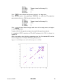
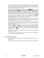
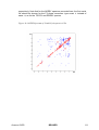
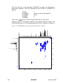
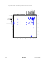
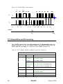
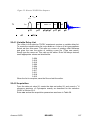
After Fourier transform, we find an all positive diagonal peak multiplet and an
anti-phase cross peak multiplet of four peaks each.
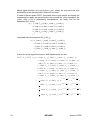
2.11 Summary and Useful Formulae
2.11.1
Effects on Spins in the Product Operator Formalism
Effect of pulses on magnetization:
βx
I z →
I z cos β − I y sin β
β
y
I z →
I z cos β + I x sin β
βx
I x →
Ix
β
y
I y →
Iy
β
y
I x →
I x cos β − I z sin β
βx
I y →
I y cos β + I z sin β
If the flip angle β = 90° then:
y ,x
I z 

→ ± I x, y
90
y,x
I x, y 

→ mIz
90
Effect of chemical shift on magnetization:
⋅ I z ⋅t
I z δ
→ I z
δ ⋅I z ⋅t
I x 
→ I x cos(δ t ) + I y sin( δ t )
δ ⋅I z ⋅t
I y 
→ I y cos(δ t ) − I x sin( δ t )
Avance 1D/2D
BRUKER
25
Effect of scalar coupling on magnetization:
2π J 12 I1 z I 2 z t
I 1z 
 → I 1z
2π J 12 I1 z I 2 z t
I 1x 
 → I 1x cos(πJ 12 t ) + 2 I 1 y I 2 z sin(πJ 12 t )
2π J 12 I1 z I 2 z t
I 1 y 
 → I 1 y cos(πJ 12 t ) − 2 I 1x I 2 z sin(πJ 12 t )
2π J 12 I1 z I 2 z t
2 ⋅ I 1x I 2 z 
 → 2 I1x I 2 z cos(πJ 12 t ) + I 1 y sin(πJ 12 t )
2π J 12 I1 z I 2 z t
2 ⋅ I 1 y I 2 z 
 → 2 I1 y I 2 z cos(πJ 12 t ) − I 1x sin(πJ 12 t )
2π J 12 I1 z I 2 z t
2 ⋅ I1x I 2 y 
 → 2 I1x I 2 y
2.11.2
Mathematical Relations and other Information
The Euler relations where used extensively in the previous paragraphs:
ei ⋅ω ⋅t = cos(ω ⋅ t ) + i ⋅ sin(ω ⋅ t )
e − i ⋅ω ⋅t = cos(ω ⋅ t ) − i ⋅ sin(ω ⋅ t )
1
cos(ω ⋅ t ) = (ei ⋅ω ⋅t + e − i ⋅ω ⋅t )
2
i
sin(ω ⋅ t ) = − (ei ⋅ω ⋅t − e − i ⋅ω ⋅t )
2
Frequently used simplifications in 2D:
− i ⋅ cosα + sin α = −i ⋅ cosα − i 2 ⋅ sin α
= −i (cosα + i ⋅ sin α )
= −i ⋅ ei ⋅α
1 i ⋅α ⋅t
(e + e − i ⋅α ⋅t ) ⋅ ei ⋅ β
2
1
= (ei ( β +α )⋅t + e i ( β −α )⋅t )
2
cosα ⋅ ei ⋅ β =
i
sin α ⋅ e i⋅β = − (e i⋅α ⋅t − e −i⋅α ⋅t ) ⋅ e i⋅β
2
i
= − (e i ( β +α )⋅t − e i ( β −α )⋅t )
2
The sensitivity of NMR experiments is given by the signal to noise ratio:
Nγ excT2 (γ det B0 )
S/N =
T
3/ 2
S/N
N
γexc
γdet
ns
26
=
=
=
=
=
ns
signal to noise ratio
number of spins in the system (sample concentration)
gyromagnetic ratio of the excited nucleus
gyromagnetic ratio of the detected nucleus
number of scans
BRUKER
Avance 1D/2D
B0
T2
T
=
=
=
external magnetic field
transverse relaxation time (determines the line width)
sample temperature
(Comment: here we can already see that it might be useful for a better signal
to noise ratio to excite one kind of nuclei and detect another kind with a better
gyromagnetic ratio in the same experiment. This is done in inverse
experiments which are described in sections 15 to 17).
2.12 Useful Coupling Constants
Many NMR constants such as chemical shift ranges, sensitivities, common
NMR solvent properties etc. can be found in the Bruker Almanac. Here we
added the values of some common coupling constants that are used more
often as parameters (cnst1 – cnst5) in some pulse programs.
2.12.1
n
JCH Coupling Constants
As a rule of thumb it is possible to estimate the 1JCH coupling constant from
the following equation: 1JCH ~ 500*(fractional CH s character). That is: 125Hz
< 1JCH < 250Hz, so that 1JCH = 145Hz is a good approximation in most cases.
The values of 2JCH coupling constants increase with increasing HCαCβ
angles and with the electronegativity of the Cβ substituent. They vary
between –5 and 50Hz.
The 3JCH coupling constants are mostly positive and are maximal at CCCH
angles of 0° and 180°. The values for trans couplings are larger as for cis
couplings (Karplus relation).
Table 2: Useful CH Coupling Constants
Avance 1D/2D
Compound
Ethane
Acetonitrile
Ethene
Benzene
Dichloromethane
Chloroform
Formaldehyde
1
System
C(sp3)C(sp3)H
C(sp3)C(sp2)H
C(sp2)C(sp3)H
C(sp2)C(sp2)H
2
JCH in Hz
-10 to +6
0 to +30
-7 to -4
-4 to +14
System
C(sp3)C(sp3)C(sp3)H
C(sp3)C(sp2) C(sp2)H
C(sp2)C(sp2) C(sp3)H
3
JCH in Hz
124.9
136.0
156
159
178.0
209.0
222.0
JCH in Hz
0 to 8
0 to 20
0 to 20
Jtrans > Jcis
BRUKER
27
2.12.2
n
JHH Coupling Constants of Hydrocarbons
Usually 2JHH coupling constants are negative and vary in a range between
-0.5Hz and -15Hz in hydrocarbons. 3JHH coupling constants are mostly
positive and usually range from 2 up to 18Hz. The n>3JHH coupling is positive
or negative with smaller absolute values, that range from 0 to 3Hz. The
Karplus relation is also valid: Jtrans > Jcis.
Table 3: Useful HH Coupling Constants
2
System
HC(sp3)H
HC(sp2)H
JHH in Hz
-12 to -15
-0.5 to -3
System
HC(sp3)C(sp3)H
HC(sp3)C(sp2)H
HC(sp2)C(sp2)H
HC(sp3)CHO
HC(sp2)CHO
3
System
HC(sp3)C(sp3)C(sp3)H
HC(sp3)C(sp2)C(sp2)H
HC(sp)C(sp)C(sp3)H
4
JHH in Hz
2 to 9
4 to 10
6 to 18
1 to 3
2 to 4
JHH (abs. value) in Hz
0
0 to 3
2 to 3
Heteroatoms with considerable I or M effect can shift the J values
dramatically.
28
BRUKER
Avance 1D/2D
3 Preparing for Acqu isition
3.1 Sample Preparation
The sample quality can have a significant impact on the quality of the NMR
spectrum. The following is a brief list of suggestions to ensure high sample
quality:
•
Always use clean and dry sample tubes to avoid contamination of the
sample.
•
Always use high quality sample tubes to avoid difficulties with shimming.
•
Filter the sample solution.
•
Always use the same sample volume or solution height (recommended
values: 0.6 ml or 4 cm of solution for 5 mm sample tubes, 4.0 ml or 4 cm
of solution for 10 mm sample tubes). This minimizes the shimming that
needs to be done between sample changes.
•
Use the depth gauge to position the sample tube in the spinner. This is
discussed further in Chapter 5 ‘Sample Positioning' of the BSMS User's
Manual.
•
Check that the sample tube is held tightly in the spinner so that it does not
slip during an experiment.
•
Wipe the sample tube clean before inserting it into the magnet.
•
For experiments using sample spinning, be sure that the spinner,
especially the reflectors, are clean. This is important for maintaining the
correct spinning rate.
3.2 Bruker NMR software
There are three major tasks that are controlled by the NMR software:
acquisition, processing and plotting. The XWinNMR program is the user
interface for all of these tasks. The commands can either be called up by
selecting the menu items or by typing the appropriate command in the
command line followed by RETURN. There are many parameters that are
important for each job and they can be accessed and edited by the user.
Each individual parameter name is attached to one default parameter. Each
parameter can also be accessed directly by entering it’s name in the
command line followed by RETURN or in the eda, edp or edg window. Since
these panels contain all possible parameters and are rather large, it is often
more convenient to use somewhat more reduced parameter editor interfaces.
Avance 1D/2D
BRUKER
29
The ased command opens the panel for the acquisition parameters that are
of importance only for the selected pulse program. Here the parameters are
also commented on.
3.2.1 XWinNMR parameters and commands
A list of commonly used acquisition and processing commands and
parameter names as well as a description of the corresponding command or
parameter is given in short in the tables below.
Table 4: Data Set Editing Commands
edc, new
iexpno
wrpa
re
rep
search
wpar
rpar
create a new data set, experiment number or processing number
copy the current experiment number
a copy of the current data set is created
change experiment number only
change processing number only
find data set
save the current parameters
select and read a predefined parameter set
Table 5: Acquisition Parameters
ns
ds
td
sw
aq
o1p
o2p
rg
number of scans
number of dummy scans
Time domain, number of acquired data points
sweep width in ppm
acquisition time
transmitter frequency of f1 channel in ppm
transmitter frequency of f2 channel in ppm
receiver gain
Table 6: Acquisition and Preacquisition Commands
edhead
edprosol
edhead
ppg
spdisp
dpa
define the current probehead
define probehead specific pulse lengths and power levels (3.0)
use probehead specific pulse lengths and power levels in the
current pulse program (3.0)
configure the routing of the spectrometer
set the pulse program
open the current pulse program in a text editor window
edit all acquisition parameters
edit the acquisition parameters that are relevant for the current
pulse program
graphical display of the current pulse program
open the graphical pulse program editor (3.0)
display all status parameters for the acquisition
wbchan
wobb
atma
atmm
select the wobbling channel for tuning and matching
tuning and matching the probe
automatic tune and match the ATM probe
manually tune and match the ATM probe
edsp, edasp
pulprog
edcpul
eda
ased, as
30
BRUKER
Avance 1D/2D
edlock
lock
lockdisp
rsh
gradshim
wsh
locking parameter for probhead and solvent
automatically lock on solvent (parameters defined in edlock)
open the lock display window
select and read shim values
start the gradient shimming subprogram
save the current shim values
setres
edte
edau
stdisp
customize the XwinNMR interface
open the temperature control window
select or edit AU programs
open the shape tool
expt
rga
zg
xaua
gs
tr
estimate the experiment time
automatically adjust the receiver gain
start acquisition
start the acquisition AU program (this also starts the acquisition)
interactive adjustment of acquisition parameters
data transfer during acquisition
halt, stop
kill
stop the acquisition
kill a specific process
Table 7: Processing Parameters
si
phc0, phc1
lb
size of the real spectrum
parameters for zero order and first order phase corrections
line broadening factor for em
Table 8: Processing Parameters
Avance 1D/2D
edp
dpp
edit all processing parameters
display all status parameters for processing
ft
em
ef
phase
apk
abs
efp
Fourier transform the current data
apply exponential window function
combined command of ft and em
set the phase correction defined by phc0 and phc1
automatically phase correct the spectrum
automatically baseline correct and integrate the spectrum
combined command of ft, em and phase
sr
sref
spectral referencing
automatically calibrate the spectrum
edc2
dual
select a second and a third data processing number
invoke the dual display
edo
edg
view
xwinplot
select an output device
edit all graphics and plotting parameters
plot preview
start the plot program
BRUKER
31
Table 9: Pulse Program Specific Parameters
pl1
pl2
pl9
pl10
pl11
pl12
pl14
pl15
f1 channel - power level for pulse (default)
f2 channel - power level for pulse (default)
f1 channel - power level for presaturation
f1 channel - power level for TOCSY-spinlock
f1 channel - power level for ROESY-spinlock
f2 channel - power level for CPD/BB decoupling
f2 channel - power level for cw saturation
f2 channel - power level for TOCSY-spinlock
sp1
f1 channel - shaped pulse for selective excitation or f1 channel shaped pulse for water flipback
f1 channel - shaped pulse 180 degree or f2 channel - shaped pulse
90 degree (on resonance)
f2 channel - shaped pulse 180 degree (off resonance2) or f2
channel - shaped pulse 180 degree (adiabatic) or f1 channel shaped pulse for wet
sp2
sp7
p0
p15
p16
p17
p18
for different applications i.e. f1 channel - variable flip angle high
power pulse in DEPT
f1 channel - 90 degree high power pulse
f1 channel - 180 degree high power pulse
f2 channel - 90 degree high power pulse
f2 channel - 180 degree high power pulse
f1 channel - 90 degree low power pulse
f1 channel - 90 degree shaped pulse (selective excitation or water
flipback/watergate or wet)
f1 channel - pulse for ROESY spinlock
homospoil/gradient pulse
f1 channel - trim pulse at pl10 or pl15
f1 channel - shaped pulse (off resonance presaturation)
d0
d1
d2
d3
d4
d6
d7
d8
d9
d11
d12
d14
d16
d17
d18
d19
d20
incremented delay (2D)
[3 usec]
relaxation delay 1-5 * T1
1/(2J)
1/(3J)
1/(4J)
delay for evolution of long range couplings
delay for inversion recovery
NOESY mixing time
TOCSY mixing time
delay for disk I/O
[30 msec]
delay for power switching
[20 usec]
delay for evolution after shaped pulse
delay for homospoil/gradient recovery
delay for DANTE pulse-train
delay for evolution of long range couplings
delay for binomial water suppression
for different applications
p1
p2
p3
p4
p6
p11
32
BRUKER
Avance 1D/2D
cnst0
cnst1
cnst2
cnst3
cnst4
cnst5
cnst11
cnst12
for different applications
J (HH)
J (XH)
J (XX)
J (YH)
J (XY)
for multiplicity selection
for multiplicity selection
vc
vd
variable loop counter, taken from vc-list
variable delay, taken from vd-list
l1
l2
l3
loop for MLEV cycle (((p6*64) + p5) * l1) + (p17*2) = mixing time
loop for GARP cycle l2 * 31.75 * 4 * p9 => AQ
loop for phase sensitive 2D or 3D using States et al. or States-TPPI
method l3 = td1/2
for different applications i.e. noediff
l4
Note that the default units for pulses are microseconds (u), the units
for delays are seconds (s), but one can always enter a value combined
with a unit to define a time slot in XWinNMR. The nomenclature here
is: s = seconds, m = milliseconds and u = microseconds. For example
To set the value of d1 to 500m would define d1 to last for half a
second.
The complete information on the nomenclature and default usage of
the pulse program parameters can be found in:
$XWinNMRHome/exp/stan/nmr/lists/pp/Param.info
The nomenclature and description of the standard pulse programs and
predefined parameter sets can be found in:
$XWinNMRHome/exp/stan/nmr/lists/pp/Pulprog.info
Acquisition, processing and plotting commands can be given either in the
XWinNMR command line or via menu selection. Examples are zg, which
starts the acquisition, ft which performs a Fourier transformation on the
current data or apk which invokes the automatic phase correction.
Another possibility to manage different task in XWinNMR are AU programs.
They handle many routine jobs an can be selected or edited by the edau
command. AU programs have to be compiled before first usage. Compile and
start AU Programs by entering xau followed by the program name.
XWinNMR also offers extensive online documentation, which can be
accessed via the help menu in the XWinNMR menu bar.
3.2.2 Changes for XWinNMR 3.0
XWinNMR version 3.0 is shipped with new systems now. There are some
new commands and the handling of some pulse programs have changed
from the software version 2.6. Specific parameters or commands for
Avance 1D/2D
BRUKER
33
XWinNMR 3.0 are marked by the comment: “[use this parameter for
XWinNMR 3.0]” throughout this manual.
•
•
The XWinNMR 2.6 commands solvloop, liprosol, gpro and
prosol are replaced by the more powerful routines edprosol and
getprosol. edprosol opens a table for the definition and calculation of
power levels, pulse lengths, different delays and gradient pulse
information. The parameters can be updated for each data set by the
command getprosol.
•
The new edhead command uses the probe information from the PICS
interface of recent probeheads which can be used in XWinNMR. Each
specific PICS probe is now automatically and uniquely identified.
•
The number of different pulse programs and parameter sets were
reduced dramatically by the introduction of a new parameter in the eda
table. The parameter FnMODE controls the mode in 2D and 3D
experiments for phase sensitive detection such as TPPI, States TPPI or
others. The “mc” command has been introduced in the pulse
programming command syntax for this task. Therefore, TPPI (*tp*) and
States-TPPI (*st*) as well as absolute value type pulse programs have
been replaced by a *ph* version that uses the mc command. The mode
can be set in the FnMODE parameter in the eda table.
The usage of gradients is simplified in pulse programming since only the
gp syntax is used. Therefore the parameters cnst21 - cnst24 for
gradients are no longer valid and are replaced by corresponding gp
parameters.
For more information on general changes, please refer to the release letter of
your software packet. Information for pulse program specific changes can be
found in: $XWinNMRHome/exp/stan/nmr/lists/pp/Update.info
3.3 Tuning and Matching the Probe
In a probehead there are resonant circuits for each nucleus indicated on the
probehead label (e.g., one for 1H and one for 13C in a dual 1H/13C probehead;
one for 1H and one for a wide range of nuclei in BBO or BBI probeheads).
There is also a resonant circuit for the lock nucleus, but the standard user will
never need to adjust this, so we will ignore it in the following. Each of the
circuits has a frequency at which it is most sensitive (the resonance
frequency). Once the sample is inserted, the probehead should be tuned and
matched for these individual frequencies.
Tuning is the process of adjusting this frequency until it coincides with the
frequency of the pulses transmitted to the circuit. For example, the frequency
at which the 1H resonant circuit is most sensitive must be set to the carrier
frequency of the 1H pulses (which is sfo1 if the 1H circuit is connected to the
34
BRUKER
Avance 1D/2D
f1 channel, sfo2 if it is connected to the f2 channel, etc.). Matching is the
process of adjusting the impedance of the resonant circuit until it corresponds
with the impedance of the transmission line connected to it. This impedance
is 50 Ω. Correct matching maximizes the power that is transmitted to the coil.
A probehead is said to be tuned and matched when all of its resonant circuits
are tuned and matched. Once a probehead has been tuned and matched, it
is not necessary to retune or rematch it after slight adjustments of the carrier
frequency, since the probehead is generally tuned and matched over a range
of a couple of hundred kHz. On the other hand, large adjustments to the
carrier frequency, necessary when changing nuclei, warrant retuning and
rematching of the probehead. Thus, a broadband probe needs to be retuned
and rematched each time the heteronucleus is changed.
If you have an ATM probe, enter edsp and set the spectrometer parameters
for the channels that should be matched and tuned. For 1H on channel F1
and 13C on channel F2 enter the following values:
NUC1
NUC2
NUC3
1H
13C
OFF
This automatically sets sfo1 to a frequency appropriate for 1H and sfo2 to
the corresponding 13C frequency for tuning and matching. Exit edsp by
clicking SAVE.
Type atma. This will invoke the automatic match and tune program for all
nuclei that were selected previously in edsp. Therefore it is not necessary to
tune and match manually.
3.4 Tuning and Matching 1H (non ATM Probes)
When the NMR experiments to be performed are 1H homonuclear
experiments (e.g., 1H 1D spectroscopy, COSY, NOESY, or TOCSY), only the
1
H circuit of the probehead has to be tuned and matched.
Make sure that the sample is in the magnet, and the probehead is connected
for standard 1H acquisition. Note that there is no special configuration for
tuning and matching. Also, it is recommended to tune and match without
sample spinning.
3.4.1 Set the Parameters
In XWIN-NMR, enter edsp and set the following spectrometer parameters:
NUC1
NUC2
NUC3
1H
OFF
OFF .
This automatically sets sfo1 to a frequency appropriate for 1H tuning and
matching. There is no need to adjust sfo1 carefully now. Exit edsp by
clicking SAVE.
Avance 1D/2D
BRUKER
35
3.4.2 Start Wobbling
Tuning and matching are carried out simultaneously using XWIN-NMR.
During wobbling, a low power signal is transmitted to the probehead. This
signal is swept over a frequency range determined by the parameter wbsw
(the default value is 4 MHz) centered around the carrier frequency (i.e.,
sfo1, sfo2, etc., depending on which nucleus is being tuned/matched).
Within the preamplifier (High Performance Preamplifier Assembly or HPPR),
the impedance of the probe over this frequency range is compared to the
impedance of a 50 Ω resistor. The results are shown both on the LED display
of the HPPR and in the acquisition submenu of XWIN-NMR. Both displays
show the reflected power of the probehead versus the frequency of the
signal. The user observes either one or both of these displays while tuning
and matching the probehead.
Before starting the wobbling procedure, ensure that no acquisition is in
progress, e.g., enter stop.
Enter acqu to switch to the acquisition window of XWIN-NMR, if it is desired
to use this to monitor the tuning and matching. Notice that being in the
acquisition window slows down the wobbling procedure, so if the HPPR LED
display will be used to monitor tuning and matching, it is best to remain in the
main XWIN-NMR window and not to switch to the acquisition window.
Start the frequency sweep by typing wobb. The curve that appears in the
acquisition window is the reflected power as a function of frequency. Unless
the probehead is quite far from the correct tuning and matching, there will be
a noticeable dip in the curve. When the 1H circuit is properly tuned, the dip
will be in the center of the window, denoted by the vertical marker; and when
the circuit is properly matched, the dip will extend all the way down to the x
axis. Similar information is conveyed by the LED display on the HPPR. The
horizontal row of LED's indicates tuning and the vertical row matching. When
the circuit is properly tuned and matched, the number of LEDs is minimized.
This usually means that only green LED, are lit in both the horizontal and
vertical displays.
3.4.3 Tune and Match
Adjust the tuning and matching screws (labeled T and M) at the base of the
probehead. Note that the screws are color coded and those for the 1H circuit
are usually yellow. Also note that the screws have a limited range and
attempting to turn them beyond this range will damage the probehead.
Since there is an interplay between tuning and matching, it is generally useful
to adjust the T and M screws in an iterative fashion. Turn the M screw until
the dip is well matched at some frequency (the dip extends to the x axis and
the number of LEDs lit in the vertical HPPR display is minimized). Most likely
this will not be the desired frequency. Adjust the T screw slightly to move the
dip toward the center of the window, or equivalently, to reduce the number of
LEDs lit in the horizontal HPPR display. Rematch the dip by adjusting the M
screw again. Note that it is possible to run out of range on the M screw. If this
happens, return M to the middle of its range, adjust T to get a well matched
dip at some frequency, and walk the dip towards the correct frequency as
described above.
36
BRUKER
Avance 1D/2D
As mentioned above, ideal tuning and matching is when the dip is centered in
the window and extends to y = 0 (the x axis) on the acquisition window, or
equivalently, when the number of LED's lit on the preamplifier is minimized in
both the vertical and horizontal display.
When the 1H circuit is tuned and matched, exit the wobble routine by typing
stop. Click on return to exit the acquisition window and return to the main
window.
3.5 Tuning and Matching 13C (non ATM Probes)
Since most 13C experiments make use of 1H decoupling, besides 13C the 1H
should be tuned and matched as well. When tuning and matching a
probehead with multiple resonant circuits, it is best to tune and match the
lowest frequency circuit first. Thus, when tuning and matching a probehead
for both 1H and 13C, first do the 13C and then the 1H adjustments.
Make sure that the sample is in the magnet, and the probehead is connected
for the appropriate experiment. Also, it is recommended to tune and match
without sample spinning.
3.5.1 Set the Parameters
In XWIN-NMR, enter edsp and set the following spectrometer parameters:
NUC1
NUC2
NUC3
13C
OFF
OFF .
This automatically sets sfo1 to a frequency appropriate for
matching. Exit edsp by clicking SAVE.
13
C tuning and
3.5.2 Start Wobbling, Tune and Match
Ensure that no acquisition is in progress, enter stop.
Enter acqu to switch to the acquisition window, if this will be used to monitor
the tuning and matching.
Start the frequency sweep by typing wobb. The curve that appears in the
acquisition window is for 13C. Adjust the tuning and matching following the
guidelines given above for 1H. Notice that some probeheads (e.g., broadband
probeheads) have sliding bars instead of screws, one set labeled tuning and
another labeled matching. Set the tuning and matching sliding bars to the
values indicated for 13C on the menu. Adjust the tuning and matching bars
until the dip is well tuned and matched at some frequency as described
above for 1H.
Once the 13C circuit is tuned and matched, the 13C wobbling must be stopped
before the 1H wobbling. Exit the wobble routine by typing stop. Enter edsp,
change NUC1 to 1H, and exit by clicking SAVE. Start the 1H frequency sweep
Avance 1D/2D
BRUKER
37
by typing wobb. After a few seconds the 1H curve appears in the acquisition
window and the 1H circuit can be tuned and matched as described above.
Alternatively, if the user already has a data set in which NUC1 = 1H and
NUC2 = OFF, there is no need to redo edsp for the current data set. The
user may simply read in the 1H data set and then type wobb.
Once the probehead is tuned and matched for
routine by typing stop.
Click on
window.
13
C and 1H, exit the wobble
to exit the acquisition window and return to the main
3.6 Locking and Shimming
Before running an NMR experiment, it is necessary to lock and shim the
magnetic field.
3.6.1 Locking
To display the lock signal enter lockdisp. This opens a window in which
the lock trace appears.
The most convenient way to lock is to use the XWIN-NMR command lock.
To start the lock-in procedure, enter lock and select the appropriate solvent
from the menu. Alternatively, enter the solvent name together with the lock
command, e.g., lock cdcl3. During lock-in, several parameters such as the
lock power, the field value, and the frequency shift for the solvent are set
according to the values in the lock table. This table can be edited using the
command edlock. Note that the lock power listed in this table is the level
used once lock-in has been achieved. The field-shift mode is then selected
and autolock is activated. Once lock-in is achieved, the lock gain is set so
that the lock signal is visible in the lock window. At this point the message
“lock: finished” appears in the status line at the bottom of the window.
The lock-in procedure outlined above sets the frequency shift to the exact
frequency shift value for the given solvent as listed in the edlock table. It
also sets the field value to the value listed in the edlock table and then
adjusts it slightly to achieve lock-in (the absolute frequency corresponding to
a given ppm value no longer depends on the lock solvent). Following this
lock-in procedure, the solvent parameter in the eda table is set
automatically, which is important if you wish to use the automatic calibration
command sref (see “Spectrum Calibration and Optimization”).
The lock-phase adjustment by monitoring the sweep wiggles (i.e., while the
field is not locked but is being swept) is recommended each time the
probehead is changed, because autolock may fail. If the original phase is
reasonably close to the correct value, lock-in can be achieved and the phase
can be adjusted using autophase. Note that the lock phase for each
probehead is stored in the edlock table. In some cases, the lock power level
listed in the edlock table is set too high leading to a saturation of the lock
signal. Usually, lock-in can be achieved, but the signal oscillates due to
38
BRUKER
Avance 1D/2D
saturation. A quick fix is simply to reduce the lock power manually after lockin. However, it is better to change the power level in the edlock table. Note
that the appropriate lock power level depends on the lock solvent, the field
value, and the probehead.
3.6.2 Shimming
If the sample has been changed, the first step after locking is shimming the
magnetic field. Enter rsh and select an appropriate shim file from the menu.
Usually, only the Z and Z2 shims (and probably the X and Y) must be
adjusted while observing the lock signal. The best shim values correspond to
the highest lock level (height of the lock signal in the window). For further
discussion of shimming see Chapter 6 ‘Shim Operation' of the BSMS User's
Manual.
If you have a gradient probe, you can also use the gradient shimming tool,
which can be started by the command gradshim. For more Information,
please refer to the gradient shimming installation and users guide which is
available online in the XWinNMR help menu.
Avance 1D/2D
BRUKER
39
40
BRUKER
Avance 1D/2D
1
4 Basic H Acquisition and
Processing
4.1 Introduction
This chapter describes the acquisition and processing of a 1D 1H NMR
spectrum using the simple one-pulse NMR experiment shown in Figure 1.
The pulse sequence consists of the recycling delay, trd, the radio-frequency
(RF) pulse, and the acquisition time during which the signal is recorded. The
pulse angle is shown to be π/2, although, in practice, it is often chosen less.
The two parameters, d1 and p1, correspond to the length of the recycle
delay, trd, and the length of the RF pulse, respectively.
Note that the time intervals depicted in the pulse sequence diagrams are not
drawn to scale. For example, d1 is typically a few seconds while p1 is
typically a few microseconds in length.
Figure 1: 1D 1H NMR One-Pulse Sequence
π/2
1H
trd
¦
d1
¦ p1
acq
4.1.1 Sample
The sample used for demonstrating the basic 1D 1H experiment is 100 mg
Cholesterylacetate in CDCl 3 with 0.5 % TMS.
4.1.2 Preparation
Make sure that you have done the following steps (see also Chapter 3
‘Preparing for Acquisition'):
•
Insert a suitable probehead
•
Read in the corresponding shim file
•
Insert the sample
•
Lock the spectrometer
Avance 1D/2D
BRUKER
41
•
Optimize the Z and Z2 (and probably X and Y) shims
•
Tune and match the probehead for 1H
4.2 Spectrometer and Acquisition Parameters
Before the acquisition of a spectrum a new data set must be created. All the
spectrometer and acquisition parameters are entered within the new data set.
The spectrometer parameters are responsible for the hardware settings
necessary for configuring the spectrometer for a particular experiment. The
command edsp calls up a window in which the spectrometer parameters for
the observe and the decoupler channel(s) are set.
The acquisition parameters include all pulse sequence parameters, the
number of data points, number of scans, receiver gain, and many others.
These may be displayed and edited by entering eda. Notice that the
spectrometer parameters are also listed in the eda table. It is important to set
the spectrometer parameters before setting the acquisition parameters,
because the values from edsp automatically overwrite the corresponding
ones from the eda table.
4.3 Create a New File Directory for the Data Set
To create a new data set, type edc in the command line of the XWIN-NMR
window. This calls up a small window entitled “Current Data Parameters”.
Enter a data set name (NAME), an experiment number (EXPNO), a
processed data number (PROCNO), the disk unit (DU) where the data is
stored, the user id (USER), and the data type (TYPE). Change the
parameters as follows:
NAME
EXPNO
PROCNO
proton
1
1
Click on SAVE. This exits edc and creates the data set proton/1/1. The
message “NEW DATA SET” should now appear on the screen.
4.4 Set Up the Spectrometer Parameters
Enter edsp and set the following spectrometer parameters:
NUC1
NUC2
NUC3
42
1H
off
off
BRUKER
Avance 1D/2D
Since there is no decoupling, the only relevant spectrometer parameters are
SFO1. Click on SAVE to save the spectrometer parameters and return to the
main window. The spectrometer is now prepared to pulse and detect at the
1
H frequency.
4.5 Set Up the Acquisition Parameters
Enter eda and set the acquisition parameters as shown in Table 10, where
only the relevant parameters are listed. Note that the parameters d1, p1, and
pl1 are included in the parameter arrays D, P and PL in the eda table,
respectively. These parameters can be edited within eda, by clicking the ‘
**Array**-button next to the corresponding parameter
Table 10: Basic 1H Spectrum Acquisition Parameters
Parameter
Value
Comments
PULPROG
zg
see Figure 1 for the pulse sequence diagram
AQ_mod
DQD
If DQD is not available, use qsim
TD
32 k
32 k is a standard value for a high-resolution
1D spectrum
PARMODE
1D
One-dimensional experiment
NS
1
one scan is recorded for parameter
optimization
DS
0
no dummy scans are recorded
D1
2
the default unit for delays is seconds; entering
“2” sets a delay of 2 seconds
(click the D**Array** button)
P1
3
the default unit for pulse lengths is
microseconds; entering “3* sets a pulse length
of 3 microseconds (µs)
(click the P**Array** button)
PL1
PL1 =
power level for the p1 pulse
see also “An Important Note on Power Levels”
on page 7
(click the P**Array** button)
Avance 1D/2D
SW
50
for the first spectrum of an unknown sample
use a large spectral width; when you enter
“50” the registered value is slightly different
RG
64
suggested receiver gain
NUC1
1H
observe nucleus
O1P
15
position of the carrier frequency is 15 ppm
BRUKER
43
Click on SAVE to save the acquisition parameters and return to the main
window. Click on DONE to save the changes and return to the eda table. As
with most acquisition parameters, however, d1, p1, and pl1 can also be
edited by typing them in the command line of the main XWIN-NMR window.
As mentioned before, most of the acquisition parameters for the current pulse
program can also be entered in the ased table.
4.6 Acquisition
Enter acqu to switch to the acquisition window. While it is possible to acquire
a spectrum from the main window, the buildup of the FID can only be
observed in the acquisition window.
Enter the command rga, which performs several acquisitions and sets a
suitable value for the receiver gain (rg). Enter zg, which deletes any
previous data (‘zero') and starts the experiment (‘go'). The message scan
1/1 indicates that the spectrometer is performing the first scan and that only
one scan will be performed.
If, at any time, a submenu is entered accidentally, click on the
button
located on the button bar and then enter acqu to switch back to the
acquisition window.
If, at some point the message “DATA OUT OF WINDOW” appears, or if the
scaling is unsuitably large or small, click on the
and
buttons
located on the button bar.
4.7 Processing
After the FID has been acquired the next step is to process the acquired
data. The processing parameters are displayed and edited by entering edp.
First, Fourier transformation is performed by entering the command ft. The
number of points used to resolve the resulting spectrum is determined by the
processing parameter si (size). The spectrum consists of si real points and
si imaginary points, and thus the default setting of si is td/2, where td is
the acquisition parameter indicating the number of time domain data points.
In general, td/2 and si are numbers described by powers of 2 (2, 4, 8, 16,
32, 64, 128, ...). If si < td/2 not all the time domain data is used for the
Fourier transformation, and if si > td/2 the time domain data is zero-filled
with 2(si) before the Fourier transformation. In 1D spectroscopy, it is often
recommended to zero-fill once, i.e., to set si = td.
Check the value of si. Enter si and when prompted enter 32k (appropriate
for td = 32 k). Enter ft: The display automatically switches from the
acquisition window to the main window and displays the. The FID can still be
viewed by returning to the acquisition window. If the x axis of the Fourier
transformed spectrum is displayed in Hz, click on
to convert into a
ppm scale. If necessary, use the buttons as described above to scale the
spectrum.
44
BRUKER
Avance 1D/2D
You can zoom into a part of the spectrum by defining the appropriate 1D plot
range. Move the cursor into the display window and press the left mouse
button to tie the cursor to the spectrum. Move the cursor to one side of the
desired zoom region and click the middle mouse button to define it. Move the
cursor to the other side of the desired plot region and click the middle mouse
button again to zoom into this region. To display the whole spectrum push
the
button.
4.8 Phase Correction
Once the spectrum is Fourier transformed it must be phase corrected. Click
on
to enter the phase correction submenu. Click on
for
th
setting the reference for the 0 -order phase correction to the position of the
biggest peak in the spectrum and adjusts its phase. To adjust the 0th-order
phase manually, place the cursor on
and hold down the left mouse
button. Move the mouse until the reference peak is positive and the baseline
on either side is as flat as possible.
Most likely, the peaks on either side of the reference peak are not yet phased
correctly and require a 1st-order phase correction. To adjust the 1st-order
phase correction, place the cursor on
and hold down the left mouse
button, and move the mouse until the peaks far from the reference point are
also in-phase.
Note that it is advisable to select the reference peak for the 0th-order phase
correction near one edge of the spectrum. However, for some samples the
biggest peak will be located in the middle of the spectrum. In such cases,
click on
and define the reference peak by moving the cursor onto
the desired peak and clicking with the middle mouse button.
Once the spectrum is phased correctly, click on return to exit the submenu
and save the phase corrections by selecting Save & return. The 0th- and 1storder phase correction values are stored as processing parameters phc0
and phc1, respectively. To quit the phase correction submenu without saving
the corrections, simply click on return and select return. In either case, the
display returns to the main menu and the spectrum appears on the screen.
Note that once suitable values of phc0 and phc1 have been stored it is
possible to use them for phase correcting subsequent spectra by typing the
command pk. In addition, the Fourier transformation (ft) and the phase
correction (pk) can be performed within one step using the command fp.
4.9 Windowing
Before the Fourier transformation is performed, it is common to apply a
window (or filter) function to the time domain data. The main reason for this is
the improvement of either signal-to-noise, or resolution. Usually, for a simple
1D spectrum as described here, the signal-to-noise ratio is improved by
multiplying the FID with a simple exponential function achieved by the
command em.
Avance 1D/2D
BRUKER
45
The decay rate of the exponential function determines the amount of line
broadening. This rate is determined by the processing parameter lb (in Hz).
Enter lb and set the value to 0.3, which corresponds to an appropriate line
broadening for high-resolution 1H spectra. Enter em to perform the
multiplication, and then enter fp to Fourier transform and phase correct the
filtered data. You can also use the combined command efp, which performs
the windowing, Fourier transformation and the phasing with the previously
determined phase correction. The final spectrum should look like the one
shown in Figure 2.
Figure 2: 1H 1D Spectrum of 100 mg Cholesterylacetate in CDCl3
9.0
46
8.0
7.0
6.0
5.0
4.0
BRUKER
3.0
2.0
1.0
0.0
ppm
Avance 1D/2D
4.10 Integration
To quantitatively analyze an observed signal, the integrated intensity of the
peaks are compared within each other.
Click
to enter the integration submenu. To integrate a peak, first
move the cursor into the spectral window and click the left mouse button.
Next, click the middle mouse button once at each end of the range of
interest; the integral appears automatically. Click the left mouse button again
to release the cursor from the spectrum. An asterisk or a vertical arrow
appears next to the right end of the integral (if not, select the integral with the
left mouse button). Correct the baseline of the integral with the
buttons. Integrate the other areas or peaks in the same way.
For the calibration, select an integral (asterisk/arrow) and click on
Enter 100 to calibrate this integral to 100%. Upon return select Save & store
‘intrng' to save the integral and normalization constant and return to the
main 1D processing window.
It is also possible to compare integral values of spectra located in different
data sets: Integrate both spectra and calibrate the integral(s) in one of them,
e.g. to 100 as described above. Enter the integration mode in the second
spectrum, select the corresponding integral (asterisk/arrow) and click on the
button to display the integral value compared to the calibrated
100% of the other signal.
Avance 1D/2D
BRUKER
47
48
BRUKER
Avance 1D/2D
5 Pulse Calibration: Protons
5.1 Introduction
This chapter describes pulse calibration procedures for 1H and 13C. It is
assumed that the user is already familiar with acquisition and processing of
simple 1D NMR spectra. Appendix A (Data Sets and Selected Parameters),
which lists all data sets generated throughout this course, and Appendix B
(Pulse Calibration Results), which provides all the pulse lengths and power
levels determined during this course, maybe useful in this context.
5.2 1H Observe 90° Pulse
For the calibration of a 1H 90° pulse on the observe channel (F1), the onepulse sequence described in Chapter 4 is used. The carrier frequency (o1p)
is set onto the resonance frequency of a peak in the 1H spectrum of an
appropriate sample. This peak is monitored while the length (p1) and/or the
strength (pl1) of the RF pulse is adjusted to determine the exact conditions
for a 90° pulse.
A common sample used for the 1H pulse calibration is 0.1% Ethylbenzene in
CDCl3. Ethylbenzene shows a simple 1H spectrum with well-separated
signals, which facilitates the selection of a single resonance line. However,
due to the relatively long spin-lattice or longitudinal relaxation time (T1) of
Ethylbenzene, a long recycle delay time must be used.
5.2.1 Preparation
Insert the sample and lock the spectrometer (lock). Readjust the Z and Z2
shims until the lock level is maximal (use lockdisp). Tune and match the
probehead for 1H observation (see Chapter 3.3).
First, create a new data set. Since this will be a 1H observe experiment, it is
best to start out from a previous 1H data set, e.g., proton/1/1: Enter re
proton 1 1, then enter edc and change the following parameters:
NAME
EXPNO
PROCNO
test1h
1
1
Click on SAVE to create the data set test1h/1/1.
Enter eda and set the acquisition parameter values as shown in Table 11.
Avance 1D/2D
BRUKER
49
Table 11: 1D 1H one-pulse Acquisition Parameters
Parameter
Value
Comments
PULPROG
zg
see Figure 1 for the pulse sequence diagram.
TD
4k
NS
1
number of scans
DS
0
no dummy scans
D1
10
interscan delay (10s, because of long T1)
P1
3
start with 3µs, which should correspond to
less than a 90° pulse
PL1
power level for the p1 pulse
see “An Important Note on Power Levels” on
page 7
SW
20
start with a large spectral width of 20ppm;
which will be optimized lateron
o1p
5
will be optimized lateron
Enter rga to perform an automatic receiver gain adjustment, then enter zg to
acquire the FID, and edp to set the processing parameters as shown in
Table 12.
Table 12: 1D 1H one-pulse Processing Parameters
Parameter
Value
SI
2k
LB
1 Hz
PSCAL
global
Comments
Fourier transform the spectrum with the command ef and phase the
spectrum according to Chapter 4.8. Type sref to calibrate the spectrum and
confirm the message “no peak found in ‘sref' default calibration done”.
5.2.2 Optimize the Carrier Frequency and the Spectral Width
The carrier position (o1p) should now be set to the signal used for monitoring
the 90° pulse calibration, which is the quartet signal of the Ethylbenzene 1H
spectrum. Expand the spectrum so that only the quartet at 2.6 ppm is
displayed. Click on
to enter the calibration submenu. Click on
with the left mouse button, move the cursor to the center of the quartet and
click the middle mouse button to assign o1p to this frequency. Click on
to exit the calibration submenu and return to the main window.
Reduce the spectral width by entering swh and change the value to 1000
(Hz).
50
BRUKER
Avance 1D/2D
Enter zg to acquire a new FID using the new values for o1p and swh and
process the spectrum using the command ef.
5.2.3 Define the Phase Correction and the Plot Region
The phase correction and the spectral region plotted in the output file must
be optimized before the automation program for the pulse calibration is
executed. Phase correct the spectrum according to Chapter 4.8 in a way that
the quartet signal is positive. Expand the spectrum so that the quartet covers
approximately the central quarter of the screen. Click on
with the left
mouse button and hit return for the following three prompts, or answer them
as follows:
F1
F2
change y-scaling on display according to PSCAL?
2.8 ppm
2.4 ppm
y
The preparations are now completed and the calibration experiment can be
executed as described in the next section.
5.2.4 Calibration: High Power
For the 90° pulse calibration an automation program called paropt is used.
(Since the execution of this automation is time consuming, it is not the best
choice if the correct pulse times and power levels are already known
approximately. In such cases, the correct values are usually just checked by
acquiring 1D spectra with different pulse widths to check for maximal signal.)
The automation program is started by typing xau paropt and answering the
appearing questions as follows:
Enter parameter to modify:
Enter initial parameter value:
Enter parameter increment:
Enter # of experiments:
p1
2
2
16
The spectrometer acquires and processes 16 spectra with incrementing the
parameter p1 from 2 µsec by 2 µsec to a final value of 32 µsec. For each of
the 16 spectra, only the spectral region defined above is plotted, and all the
spectra are plotted side-by-side in the file test1h/1/999 as shown in Figure 3.
At the end of the experiment, the message “paropt finished” and a value for
the parameter p1 is displayed, which corresponds to the 90° pulse length of
the 1H transmitter with the power level as defined by pl1. Write this value
down and follow the procedure described below to obtain a more accurate
90° pulse measurement.
Return to the data set test1h/1/1 by entering re 1 1. Type p1 and enter a
value which corresponds to a 360° pulse (i.e., four times the 90° value
determined by paropt before). Acquire and process a new spectrum by typing
zg and efp (see Chapter 4.9) respectively. Change p1 slightly and acquire
and process a spectrum again, until the quartet undergoes a zero crossing as
expected for an exact 360° pulse. Note that the quartet signal is negative for
pulse angles slightly less than 360° and positive when the pulse angle is
slightly more than 360°.
Avance 1D/2D
BRUKER
51
The 360° pulse length divided by four yields the accurate 1H 90° transmitter
pulse length for the actual power level pl1.
Figure 3: Paropt Results for 1H 90° Pulse Calibration
p1 = 180°
p1 = 270°
p1 = 90°
5.2.5 Calibration: Low Power for MLEV Pulse Train (TOCSY)
The 1H 90° pulse for the MLEV pulse train used during the spinlock period of
a TOCSY sequence is between 30 µsec to 40 µsec. The procedure outlined
below uses the paropt routine to determine the corresponding power level.
However, the power level can be estimated roughly by using a rule of thumb:
The pulse length doubles for an additional 6 dB increase of the power level.
For example, the 90° pulse length (p1) was determined 8 µsec for pl1 =
0 dB. Thus, the p1 = 16 µsec for pl1 = 6 dB, or the p1 = 32 µsec for pl1 =
12 dB.
For performing the exact determination of the low power pulse, return to the
file test1h/1/1 (re 1 1). Enter p1 and change the value to 35 (µsec), type xau
paropt and answer the questions as follows:
Enter parameter to modify:
Enter initial parameter value:
Enter parameter increment:
Enter # of experiments:
pl1
0
1
16 .
Again, the 16 spectra will be displayed in the file test1h/1/999 and at the end
of the experiment, the message “paropt finished” and a value for pl1 is
52
BRUKER
Avance 1D/2D
displayed. This value corresponds to the 1H transmitter power level for a 90°
pulse length of 35 µsec. Write down this value and follow the procedure
described below to obtain a more accurate 90° pulse measurement.
Return to test1h/1/1 (re 1 1), type p1 and change the value to 140 µsec (=
360° pulse). Acquire and process a spectrum (zg, efp) by using the power
level pl1 determined by paropt above. Change pl1 slightly until the quartet
undergoes a zero-crossing indicating the accurate 360° pulse. Divide this
360° pulse time by four to get the 90° pulse length.
Note that the parameters used by the TOCSY sequence are p6 for the 90°
pulse length and pl10 for the power level, rather than p1 and pl1.
5.2.6 Calibration: Low Power for ROESY Spinlock
The power level required for the cw spinlock pulse used with ROESY
experiments corresponds to a 90° pulse length of 100 µsec to 120 µsec. As
described for the 90° pulse determination of the MLEV pulse above in
Chapter 5.2.5, the power level can again be estimated using the rule of
thumb, or measured using the paropt automation.
When using paropt, return to the file test1h/1/1 (re 1 1), enter p1 and
change the value to 110 (µsec), and type xau paropt. Answer the questions
as follows:
Enter parameter to modify:
Enter initial parameter value:
Enter parameter increment:
Enter # of experiments:
pl1
10
1
16 .
The results are displayed in the file test1h/1/999, and at the end of the
experiment, the message “paropt finished” and a value for pl1
corresponding to the 1H transmitter power level for a 90° pulse length of 110
µsec are displayed. Follow the same procedure as described in Chapters
5.2.4 and 5.2.5 for a more accurate determination of the power level.
Note that since ROESY uses cw spinlock, only the power level determination
is important here, but not the actual 90° pulse length. The power level
parameter used with the ROESY sequence is pl11, rather than pl1.
Avance 1D/2D
BRUKER
53
54
BRUKER
Avance 1D/2D
13
6 Basic C acquisition and
processing
6.1 Introduction
This chapter describes the acquisition and processing of a 13C spectrum
acquired with a one-pulse sequence with and without 1H decoupling.
6.1.1 Sample
Since NMR is much less sensitive to 13C nuclei than to 1H, it is advisable to
replace the 100 mg sample of cholesterylacetate used in chapter 3 ‘Basic 1H
Acquisition and Processing’ with a 1g sample of cholesterylacetate in CDCl3.
6.1.2 Prepare a New Data Set
Create a new data set starting from setup1h/1/1 created in the last chapter.
Enter edc and change the following parameters:
NAME
EXPNO
PROCNO
setup13c
1
1
Click on SAVE to create the data set setup13c/1/1. Enter edsp and set the
following spectrometer parameters:
NUC1
NUC2
13C
1H
Click on SAVE. The spectrometer is now ready to pulse and detect at the
frequency and to pulse and decouple at the 1H frequency.
13
C
Lock the spectrometer (lock cdcl3), adjust the Z and Z2 shims until the
lock level is optimized (use lockdisp), tune and match the probehead for
13
C and 1H.
6.2 One-Pulse Experiment without 1H Decoupling
The one-pulse sequence without decoupling is identical to the one used in
Chapter 3 (Figure 1) except that the RF pulse is applied at the 13C frequency.
Enter eda and set the acquisition parameters values as shown in Table 13.
Avance 1D/2D
BRUKER
55
Table 13: 13C Basic Acquisition Parameters
Parameter
Value
Comments
PULPROG
zg
see Figure 1 for pulse sequence diagram.
TD
64 k
NS
1
DS
0
D1
2
P1
3
the default unit for pulse lengths is microseconds; entering “3” sets a pulse length of 3
microseconds
high power level on F1 channel (13C)
PL1
see also “Important note on power levels”
SW
250
13
O1P
100
will be optimized later
C spectra cover a much broader spectral
range than 1H spectra
Enter rga to start the automatic receiver gain adjustment and then zg to
acquire the FID.
Type si and enter a value of 32k. Type lb and enter 3. Enter ef to add line
broadening and Fourier transform the data. Manually phase correct the
spectrum and store the correction. Subsequent 13C spectra can now be
processed with the command efp, which combines the exponential
multiplication, Fourier transformation, and phase correction using the stored
phc0 and phc1 values.
The processed spectrum is very noisy and most likely only one single peak is
visible arising from the CDCl3 solvent as shown in Figure 4. Type sref to
calibrate the spectrum correctly. Note that the sref command works
properly only if the parameter solvent is set to the correct solvent in the
eda table.
The signal-to-noise ratio is improved by acquiring more than one scan.
Enter edc and set EXPNO to 2. Click on SAVE to create the data set
setup13c/2/1.
Enter ns (number of scans) and change the current value to 64. Enter ds
(dummy scans) and change the current value to 4. The four dummy scans
ensure that the system reaches steady state conditions before any spectra
are added together. Enter zg to acquire the FID and efp to add line
broadening, Fourier transform, and phase correct the data after the
acquisition is completed. As shown in Figure 5, more peaks are visible now.
However, the signal-to-noise ratio still is unsatisfactory.
The 13C carrier frequency must be adjusted and set to the center of the
spectrum. To do so, click on the button
to enter the calibration
56
BRUKER
Avance 1D/2D
submenu, and then
with the left mouse button to select o1p calibration.
Tie the cursor to the spectrum, move it to the Chloroform peak and press the
middle mouse button to set o1p to this frequency. Click on
. Acquire
and process another spectrum with this new o1p (zg, efp).
Figure 4: 13C spectrum of 1 g cholesterylacetate in CDCl3
150
100
50
0
-50
-100
ppm
The signal-to-noise ratio can be improved further by the application of 1H
decoupling as shown in the next section.
Figure 5: 13C spectrum of 1 g cholesterylacetate in CDCl3
150
Avance 1D/2D
100
50
0
BRUKER
-50
-100
ppm
57
6.3 One-Pulse Experiment with 1H Decoupling
The one-pulse sequence with 1H decoupling is shown in Figure 6. In addition
to the one-pulse sequence used before, 1H is decoupled throughout the
entire length of the pulse program.
Figure 6: 13C One-Pulse Sequence with 1H Decoupling
π/2
13C
trd
d1
¦
1H
¦ p1
acq
decoupling
Before acquiring a 1H-decoupled 13C spectrum, the frequency of the 1H
signals in must be determined. Figure 2 (Section 3.9) shows a 1H spectrum
of cholesterylacetate (or look it up with re setup1h 1 1): Most 1H signals
lie in the range of 0.5 to 5.5 ppm. An appropriate frequency for 1H decoupling
would therefore be 3 ppm. In general, 5 ppm is a safe frequency to select for
1
H decoupling if no 1H spectrum is available.
In case you looked up the 1H spectrum (data set proton/1/1), return to the
previous carbon spectrum by entering re setup13c 3 1. Enter edc, set
EXPNO to 3 and click on SAVE to create the data set setup13c/3/1.
Enter eda and set the acquisition parameters as shown in Table 14.
Table 14: 13C Acquisition Parameters for 1H Decoupled Spectrum
Parameter
Value
Comments
PULPROG
zgdc
see Figure 6 for pulse sequence diagram.
TD
32k
NS
1
DS
0
D1
2
should be 1–5*T1(13C).
P1
3
the default unit for pulse lengths is microseconds; entering “3” sets a pulse length of 3
microseconds
PL1
13
power level for the p1 pulse ( C)
See also “Important note on power levels”
58
BRUKER
Avance 1D/2D
1
Pl12
low power level on F2 channel ( H) as
determined in Section 4.2.6 for ROESY spin
lock
PCPD2
1
SW
H 90° pulse for cpd sequence as determined
in Section 4.2.6
350 ppm
O1P
frequency of
Section 5.2
13
C carrier as optimized in
O2P
3
frequency of 1H carrier
CPDPRG2
waltz16
1
H decoupling sequence
Enter zg to acquire an FID.
Enter efp to perform line broadening, Fourier transformation, and phase
correction. A 1H decoupled 13C spectrum is shown in Figure 7. Note the
improved signal-to-noise ratio.
Figure 7: 13C spectrum of 1 g cholesterylacetate in CDCl3 with 1H decoupling
200
Avance 1D/2D
150
100
50
BRUKER
0
-50
ppm
59
60
BRUKER
Avance 1D/2D
7 Pulse Calibration: Carbon
7.1 13C Observe 90° Pulse
The 13C observe pulse calibration experiment requires a sample with a strong
13
C signal, e.g., 80% Benzene in Acetone-d6. If no appropriate sample is
available, the inverse mode 13C pulse calibration procedure described in
Section 7.3 can be used instead.
7.1.1 Preparation
Insert the sample and lock the spectrometer (lock). Readjust the Z and Z2
shims until the lock level is maximal (use lockdisp). Tune and match the
probehead for 13C observation and 1H decoupling (see Chapter 3.5). Create a
new data set: Enter re proton 1 1, enter edc and change the following
parameters:.
NAME
EXPNO
PROCNO
test13c
1
1.
Click on SAVE to create the data set test13c/1/1.
Enter edsp and set NUC1 to 13C, turn off NUC2 and press the DEFAULT
button, then click on SAVE.
Enter eda and set the acquisition parameters as shown in Table 15.
Table 15: 1D 1H one-pulse Acquisition Parameters
Parameter
Value
Comments
PULPROG
zg
see Figure 1 for pulse sequence diagram.
TD
4k
NS
1
DS
0
D1
20
interscan delay (20s, because of long T1)
P1
3
start with 3µs, which should correspond to
less than a 90° pulse
PL1
power level for the p1 pulse
see “An Important Note on Power Levels” on
page 7
SW
o1p
Avance 1D/2D
350
start with a large spectral width of 350ppm;
which will be optimized lateron
start with 100ppm, it will be optimized later
BRUKER
61
Enter rga to perform an automatic receiver gain adjustment; enter zg to
acquire the FID, and edp to set the processing parameters as shown in
Table 16.
Table 16: 1D 13C one-pulse Processing Parameters
Parameter
Value
SI
2k
LB
3 Hz
PSCAL
global
Comments
Add line broadening and Fourier transform the spectrum with the command
ef. Manually phase correct the spectrum and store the correction.
Type sref to calibrate the spectrum and confirm the message “no peak
found in ‘sref' default calibration done”.
7.1.2 Optimize the Carrier Frequency and the Spectral Width
The carrier frequency should now be set to the signal used to calibrate the
90° pulse: Expand the spectrum until only the doublet at 130 ppm is
displayed. Enter the calibration submenu by clicking
. Click on
with the left mouse button and move the cursor to the center of the doublet.
Click the middle mouse button to assign o1p to this frequency. Click
to exit the calibration submenu and return to the main window.
Reduce the spectral width by entering swh and change the value to 1000
(Hz). Acquire and Fourier transform another spectrum (zg, ef).
7.1.3 Define the Phase Correction and the Plot Region
Now it is necessary to define the phase correction and spectral region that
will be plotted in the output file produced by paropt. Phase correct the
spectrum so that the doublet is positive. Expand the spectrum so that the
doublet covers approximately the central third of the screen. Click on
with the left mouse button and answer the three questions as follows:
F1
F2
change y-scaling on display according to PSCAL?
133 ppm
127 ppm
y
7.1.4 Calibration: High Power
As for the 1H 90° calibration (Chapter 5.2.4), the automation program paropt
is used. Type xau paropt and answer the questions as follows:
Enter parameter to modify:
Enter initial parameter value:
Enter parameter increment:
Enter # of experiments:
62
BRUKER
p1
2
2
16
Avance 1D/2D
Paropt acquires and processes 16 spectra while incrementing the parameter
p1 from 2 µsec to 32 µsec. The result is displayed side-by-side in
test13c/1/999 and should resemble Figure 8. At the end of the experiment,
the message “paropt finished” appears and a value for p1 is displayed, which
corresponds to the 90° pulse length of the 13C transmitter using the current
power level pl1. Write this value down and follow the procedure below to
obtain a more accurate 90° pulse measurement.
Return to the data set test13c/1/1 by entering re 1 1. Type p1 and enter a
value corresponding to a 360° pulse (i.e., four times the 90° value
determined by paropt above). Acquire and process another spectrum (zg,
efp). Change p1 slightly, acquire and process a spectrum again, until the
doublet shows a zero-crossing indicating the 360° pulse. The 360° pulse time
divided by 4 is the exact 90° pulse length for the 13C transmitter for the power
level pl1.
Note that the probe may arc, if the 90° pulse length is less than 5 µsec for
5 mm probes and less than 10 µsec for 10 mm probes. In this case the pl1
must be set to a higher value (increase the attenuation on the transmitter)
and the corresponding 90° pulse length must be determined again.
Figure 8: Paropt Results for 13C 90° Pulse Calibration
p1 = 180°
p1 = 270°
p1 = 90°
7.2 1H Decoupling 90° Pulse During 1 3 C Acquisition
Ideally, this procedure is carried out immediately following the 13C observe
pulse calibration described above, since the magnet is then locked and
shimmed, and the probehead is tuned and matched for both 13C and 1H.
Avance 1D/2D
BRUKER
63
7.2.1 Sample
For the 1H decoupling pulse calibration, the sample must yield a 13C signal of
reasonable intensity with a detectable scalar 13C–1H coupling: Therefore,
80% Benzene in Acetone-d6 is a good choice.
7.2.2 Pulse Sequence
The pulse sequence used is called DECP90 and it is shown in Figure 9. The
sequence consists of a recycle delay (trd, d1) followed by a 90° 13C pulse
(p1), a delay 1/[2J(13C,1H)] (d2, cnst2) for the evolution of antiphase 13C–1H
magnetization, a 1H pulse (p3), and the 13C detection period (acq, aq). For
the calibration of the 90° 1H decoupling pulse, the length (and/or the strength)
of the 1H pulse p3 (and/or the power level pl2) is adjusted. No signal is
acquired for an exact 1H 90° pulse p3, since only undetectable multiple
quantum coherence 13C magnetization is present.
Figure 9: DECP90 Pulse Sequence
π/2
13
C
1/[2J(13C,1H)]
trd
d1
p1
d2
acq
p3
1
H
7.2.3 Set the 1H Carrier Frequency
The first spectrum will be a 1H observe experiment to determine the correct
frequency for the DECP90 1H decoupling pulse. Create a new data set
starting from e.g., proton/1/1 (re proton 1 1), enter edc and change the
following parameters:
NAME
EXPNO
PROCNO
testdec
1
1
Click on SAVE to create the data set testdec/1/1 and enter eda to set the
acquisition parameters as shown in Table 17.
Table 17: 1D 1H one-pulse Acquisition Parameters
64
Parameter
Value
Comments
PULPROG
zg
see Figure 1 for the pulse sequence diagram.
BRUKER
Avance 1D/2D
TD
4k
NS
1
DS
0
D1
10
interscan delay (10s, because of long T1)
P1
3
start with 3µs, which should correspond to
less than a 90° pulse
high power level on F1 channel (1H) as
determined in Section 5.2.4
PL1
SW
20
o1p
5
start with a large spectral width of 20ppm;
which will be optimized lateron
Enter rga, zg and edp to perform an automatic receiver gain adjustment,
acquire an FID, and set the processing parameters as shown in Table 18.
Table 18: 1D 1H one-pulse Processing Parameters
Parameter
Value
SI
2k
LB
1
PSCAL
global
Comments
Type the command ef to perform line broadening and Fourier
transformation, and phase correct the spectrum. Type sref to calibrate the
spectrum and confirm the message “no peak found in ‘sref' default calibration
done”.
Click the left mouse button with the cursor placed in the spectral field of the
main window. Move the cursor to the top of the Benzene peak at around
7.3 ppm and note the exact ppm-value of the cursor position in the small
“Info” window. Click the left mouse button to release the cursor from the
spectrum.
7.2.4 Set the 13C Carrier Frequency and the Spectral Width
These parameters were already determined for the data set test13c/1/1. To
transfer all the parameters from test13c/1/1 to the new data set, enter re
test13c 1 1, enter edc and change the following parameters:
NAME
EXPNO
PROCNO
testdec
2
1
Click on SAVE to create the data set testdec/2/1.
Since now 1H decoupling is required, enter edsp and set NUC2 to 1H so that
the spectrometer parameters are as follows:
Avance 1D/2D
BRUKER
65
NUC1
NUC2
(NUC3
13C
1H
off)
Enter eda and set the acquisition parameters values as shown in Table 19.
The parameters o1p and swh should be set as used in test13c/1/1. Set o2p
to the exact 1H offset frequency determined in the previous section (around
7.3ppm). The DECP90 experiment will not work as described below unless
both o1p and o2p are set correctly.
Table 19: DECP90 Acquisition Parameters
Parameter
Value
PULPROG
decp90
TD
4k
NS
1
DS
0
Comments
see Figure 9 for pulse sequence diagram.
PL1
high power level on F1 channel (13C) as
determined in Section 7.1.4
PL2
high power level on F2 channel (1H) as
determined in Section 5.2.4
P1
13
C 90° pulse as determined in Section 7.1.4
P3
3
start with 3µs, which should correspond to
less than a 90° pulse
D1
5
interscan delay (5s, because of long T1)
CNST2
160 Hz
heteronuclear scalar J(13C,1H) coupling
D2
3.125 msec
1/[2J(13C,1H)]
(calculated automatically from cnst2 above)
SWH
1000 Hz
o1p
13
o2p
1
C offset as determined in Section 7.1.2
H offset as determined in Section 7.2.3
Enter zg to acquire the FID (the receiver gain should already be set
appropriately), enter edp and verify the processing parameters as shown in
Table 20.
Table 20: DECP90 Processing Parameters
66
Parameter
Value
SI
2k
LB
1 Hz
PSCAL
global
Comments
BRUKER
Avance 1D/2D
Fourier transform the spectrum with line broadening by the command ef.
Manually phase correct the spectrum so that the left peak is positive and the
right peak is negative, and store the correction.
The spectrum is already calibrated if the current data set was created from
test13c/1/1. Since paropt is not used here, neither the phase correction nor
the plot region have to be defined.
7.2.5 Calibration: High Power
The 1H 90° decoupling pulse length should be close to the 1H 90° observe
pulse length for the same power level: Set p3 to the value found in Section
5.2.4 and acquire and process a spectrum (zg, efp). If the 1H 90° pulse (p3)
is less than 90°, the left peak will be positive and the right peak negative. If
the pulse angle is between 90° and 270°, the phase of the two peaks will be
opposite. If the p3 pulse length corresponds to a 90° pulse, the signals show
a zero-crossing as shown in Figure 10.
Figure 10: 1H Decoupling 90° Pulse Calibration
p3 > 90°
p3 = 90°
p3 < 90°
133
131
129
127
ppm
7.2.6 Calibration: Low Power for WALTZ-16 Decoupling
The WALTZ-16 composite pulse decoupling (cpd) sequence requires a 1H
90° decoupling pulse length of 80 to 100 µsec. Adjust pl2 and p3 to
determine the 90° pulse length in this range. Make use of the rule of thumb:
90° pulse length approximately doubles for an additional 6 dB increase in
attenuation.
Avance 1D/2D
BRUKER
67
Note that the parameters used by cpd sequences are pcpd2 for the 90°
pulse length and pl12 for the decoupler power level, rather than p3 and pl2
as used here.
7.3 13C Decoupler 90° Pulse (Inverse Mode)
This calibration procedure should yield approximately the same pulse length
as for the 13C observe 90° pulse (Section 7.1.4). However, the method
described here is more convenient because of the more sensitive 1H
detection instead of 13C. In addition, the T1 of 1H is shorter than for 13C, which
allows the selection of shorter interscan delays.
7.3.1 Sample
For these so-called inverse experiments, the detected nucleus is 1H, but 13C
satellites must be visible. Therefore, a convenient sample is the 1H
Lineshape Sample (3% Chloroform in Acetone-d6 for frequencies between
300 MHz and 500 MHz, and 1% Chloroform in Acetone-d6 for frequencies
>600 MHz). Here the procedure is described for this readily available
standard sample. However, use the “Pulse Calibration” sample containing
0.1M 13C-methanol and 0.1M 15N-urea in DMSO-d6, if this is available.
The same DECP90 pulse sequence as used for the 1H 90° decoupling pulse
determination in Section 7.2 is used here, except that the 1H and 13C
channels are interchanged as shown in Figure 11.
Figure 11: DECP90 Pulse Sequence
π/2
1
H
1/[2J(13C,1H)]
trd
d1
p1
d2
acq
p3
π/2
13
C
7.3.2 Preparation
Insert the sample, lock the spectrometer, readjust the Z and Z2 shims until
the lock level is optimized, tune and match the probehead for 1H observation
and 13C decoupling.
68
BRUKER
Avance 1D/2D
7.3.3 Set the 13C Carrier Frequency
First, a 13C observe experiment is recorded to determine the correct 13C
carrier frequency (which is o1p here but will be o2p in the inverse calibration
experiment).
Create a new data set starting from a previous 13C data set, e.g., carbon/1/1
(re carbon 1 1), enter edc and change the following parameters:
NAME
EXPNO
PROCNO
testinv
1
1
Click on SAVE to create the data set testinv/1/1. Type edsp and set the
parameters as follows for observing 13C and decoupling 1H:
NUC1
NUC2
(NUC3
13C
1H
off)
Click on SAVE to save the spectrometer parameters and return to the main
window and enter eda to set the acquisition parameters as shown Table 21.
Table 21: 1D 13C One-pulse Acquisition Parameters
Parameter
Value
PULPROG
zgdc
TD
4k
NS
1
DS
0
Comments
PL1
high power level on F1 channel (13C) as
determined in Section 7.1.4
PL12
low power level on F2 channel (1H) for cpd as
determined in Section 7.2.6
P1
3
start with less than a 90° pulse
1
PCPD2
H 90° pulse for cpd sequence as determined
in Section 7.2.6
D1
5
SWH
1000
RG
4k
o1p
77ppm
o2p
5
CPDPRG2
waltz16
Chloroform resonance
cpd sequence for the 1H decoupling
Notice that the spectral width (swh) is much smaller than usually used for 13C
spectra, because only the chloroform signal must be recorded and o1p is set
to almost the correct frequency in this data set.
Avance 1D/2D
BRUKER
69
Enter zg to acquire the FID. Enter edp and set the processing parameters as
shown in Table 22.
Table 22: 1D 13C One-pulse Processing Parameters
Parameter
Value
SI
2k
LB
1 Hz
PSCAL
global
Comments
Fourier transform the data (ef) and phase the spectrum manually. Type
sref to calibrate the spectrum and confirm the message “no peak found in ‘
sref' default calibration done”.
Expand the spectrum until only the chloroform signal at 77 ppm is displayed.
Enter the calibration submenu by clicking
. Click on
with the
left mouse button and move the cursor to the center of the signal. Click the
middle mouse button to assign o1p to this frequency. Click
to exit
the calibration submenu and return to the main window. This o1p value will
be the 13C o2p value for the DECP90 pulse sequence below.
7.3.4 Set the 1H Carrier Frequency and the Spectral Width
Now, a 1H observe experiment to determine the correct offset for 1H (o1p)
must be recorded: Create a new 1H data set starting from a previous one,
e.g., proton/1/1 (re proton 1 1). Enter edc and change the following
parameters:
NAME
EXPNO
PROCNO
testinv
2
1
Click on SAVE to create the data set testinv/2/1, then enter eda and change
the acquisition parameters as shown in Table 23.
70
BRUKER
Avance 1D/2D
Table 23: 1D 1H One-pulse Acquisition Parameters
Parameter
Value
Comments
PULPROG
zg
see Figure 1 for pulse sequence diagram.
TD
8k
NS
1
DS
0
high power level on F1 channel (1H) as
determined in Section 5.2.4
PL1
P1
3
D1
5
SW
20 ppm
o1p
5
1
H pulse (less than a 90° pulse)
Enter rga to perform an automatic receiver gain adjustment, zg to acquire
the FID and edp to set the processing parameters as shown in Table 24.
Table 24: 1D 1H One-pulse Processing Parameters
Parameter
Value
SI
4k
LB
0.3 Hz
PSCAL
global
Comments
Fourier transform the data (ef) and phase correct the spectrum. Type sref
to calibrate the spectrum and confirm the message “no peak found in ‘sref'
default calibration done”.
Expand the spectrum until only the chloroform signal at 7.2ppm is displayed
and set the o1p value exactly on the methanol peak in the
menu
(follow the same procedure as described in Section 5.2.2). The spectral width
(swh) can now be reduced to 1000 Hz.
7.3.5 Preparations for the Inverse Pulse Calibration
The correct 1H and 13C frequencies have now been determined. Next, a
DECP90 spectrum is acquired to determine the appropriate phase correction
values. Create a new data set by entering edc and change EXPNO to 3.
Click SAVE to create the data set testinv/3/1.
Enable 13C decoupling by entering edsp and set the following spectrometer
parameters:
Avance 1D/2D
BRUKER
71
NUC1
NUC2
NUC3
1H
13C
off
Click on SAVE to save the spectrometer parameters and return to the main
window. Set o2p to the o1p value of the 13C determined in Section 7.3.3.
Enter eda and set the acquisition parameters as shown in Table 25.
Table 25: DECP90 Acquisition Parameters
Parameter
Value
Comments
PULPROG
decp90
see Figure 11 for pulse sequence diagram.
TD
8k
NS
1
DS
0
1
PL1
high power level on F1 channel ( H) as
determined in Section 5.2.4
PL2
high power level on F2 channel (13C) as
determined in Section 7.1.4
P1
1
H 90° pulse as determined in Section 5.2.4
P3
0
for the phase correction, do not use p3
D1
5
relaxation delay; should be 1–5 * T1(1H).
CNST2
214
heteronuclear scalar J(13C,1H) coupling [Hz]
D2
3.34ms
1/[2J(13C,1H)]
(calculated automatically from cnst2 above)
SWH
1000 Hz
RG
use value from testinv/2/1.
o1p
~7.24ppm
1
o2p
~77ppm
13
H offset frequency of chloroform peak as
determined in Section 7.3.4
C offset frequency of chloroform peak as
determined in Section 7.3.3
Enter zg to acquire the FID and enter edp to set the processing parameters
as shown in Table 26.
Table 26: DECP90 Processing Parameters
72
Parameter
Value
SI
4k
LB
0.3 Hz
PSCAL
global
Comments
BRUKER
Avance 1D/2D
Fourier transform the spectrum (ef). Expand the spectrum to display the
region between 8.5 to 7.5 ppm, in the region of the chloroform peak with it’s
two 13C satellites. Correct the phase in a way that the left satellite is positive
and the right satellite is negative.
7.3.6 Calibration: High Power
Set p3 to the value obtained with the direct method in Section 7.1. Acquire
and process another spectrum (zg, efp). If the pulse is less than 90°, the left
satellite will remain positive and the right satellite negative. If the pulse angle
is between 90° and 270°, the two satellite signals will show opposite phase. If
the p3 pulse corresponds to 90°, the satellites show a zero-crossing (Figure
12).
Figure 12: 13C Decouple 90° Pulse Calibration Results on the chloroform sample
p3 > 90°
p3 = 90°
p3 < 90°
8.5
8.3
8.1
7.9
7.7
ppm
7.3.7 Calibration: Low Power for GARP Decoupling
The GARP composite pulse decoupling (cpd) sequence requires a 90°
decoupling pulse length of 60 to 70 µsec. Adjust pl2 and p3 to determine
the combination that yields a 90° pulse length in this range. Use the rule of
thumb: The pulse length doubles for a 6 dB increase in attenuation.
Avance 1D/2D
BRUKER
73
Note that the parameters used by cpd sequences are pcpd2 for the 90°
pulse length and pl12 for the decoupler power level, rather than p3 and pl2
as used here.
7.4 1D Inverse Test Sequence
The 1D HMQC pulse sequence shown in Figure 13 is used to check the
parameters for inverse experiments. This experiment detects only signals of
protons directly attached to 13C nuclei, whereas the signal arising from
protons attached to 12C is suppressed by phase cycling. Thus, the 1D HMQC
spectrum of the current sample (10% Chloroform in Acetone-d6) yields only
signal from the 13C satellites without the large central peak.
Figure 13: 1D HMQC Pulse Sequence
π/2
1H
π
trd
p1
¦ d1
13C
π/2
p2
π/2
d2
d2
1/(2JXH)
acq
1/(2JXH)
p3
p3
Create a new data set starting from testinv/3/1 (re testinv 3 1), enter
edc and set EXPNO to 4. Click SAVE to create the data set testinv/4/1. Enter
eda and set the acquisition parameters as shown in Table 27.
Table 27: 1D HMQC Acquisition Parameters
74
Parameter
Value
Comments
PULPROG
inv4ndrd1d
TD
8k
NS
16
the number of scans should be 4 * n in order
for the phase cycling to work properly.
DS
16
number of dummy scans.
see Figure 13 for pulse sequence diagram.
1
PL1
high power level on F1 channel ( H) as
determined in Section 5.2.4
PL2
high power level on F2 channel (13C) as
determined in Section 7.1.4
BRUKER
Avance 1D/2D
P1
1
P2
1
P3
13
H 90° pulse as determined in Section 5.2.4
H 180° pulse: set to 2*P1
C 90° pulse as determined in Section 7.3.6
D1
20 sec
relaxation delay; should be 1–5 * T1(1H).
CNST2
214
heteronuclear scalar J(13C,1H) coupling [Hz]
Enter zg to acquire the FID and edp to set the processing parameters as
shown in Table 28.
Table 28: 1D HMQC Processing Parameters
Parameter
Value
SI
4k
WDW
EM
LB
0.30 Hz
PKNL
TRUE
Comments
necessary when using the digital filter.
Fourier transform the data (ef) and phase correct the spectrum.
A 1D HMQC spectrum of Chloroform is shown in Figure 14. Note that the
phase cycling is not as perfect to completely suppress the main signal arising
from 1H directly attached to 12C, due to technical limitations
.
Avance 1D/2D
BRUKER
75
Figure 14: 1D HMQC Spectrum of Chloroform
8.7
76
8.5
8.3
8.1
7.9
BRUKER
7.7
7.5
ppm
Avance 1D/2D
8 Advanced 1D
13
C Experiments
8.1 13C Experiments with Gated 1H-Decoupling
In principle, the values for scalar couplings between 1H and 13C, and the
signal multiplicity can give additional information for the structure
determination. The disadvantages of not decoupling 1H in 13C spectra are the
decreased sensitivity due to the distribution of the signal intensity into the
different lines of the multiplet, the signal overlap, and the missing NOE effect.
This chapter describes the acquisition and processing of 13C spectra
acquired with commonly used 1H decoupling techniques called ‘gateddecoupling’ and ‘inverse gated-decoupling’.
The gated-decoupled 13C spectrum is recorded with 1H decoupling during the
relaxation delay, whereas the decoupling is switched off during 13C
acquisition.
For the inverse gated-decoupling experiment the 1H decoupling is active
during the acquisition, whereas it is switched off during the relaxation delay.
The sensitivity improvement due to the NOE-effect is suppressed for this
experiment and thus the acquired spectrum can be integrated. Note that
there is a build up of the NOE-effect during the acquisition period when
decoupling is active. In order to suppress this NOE-effect the relaxation delay
must be 10-times the T1 relaxation time for 13C.
The pulse sequences for the gated-decoupling and the inverse gateddecoupling experiments are shown in Figure 15 and Figure 16, respectively.
However, before acquiring a 1H-decoupled 13C spectrum, the frequencies of
the cholesterylacetate 1H signals must be determined. See Section 6.3 for
the determination of the exact 1H carrier frequency. As a rule of thumb,
5 ppm is a safe frequency to select for 1H decoupling when no optimized 1H
spectrum is available.
Figure 15: 13C Pulse Sequence with Gated 1H Decoupling
π/2
13C
trd
¦
1H
Avance 1D/2D
d1
¦ p1
acq
decoupling
BRUKER
77
Return to the carbon/3/1 data set by entering re carbon 3 1. Enter edc and
set EXPNO to 4. Click on
to create the data set carbon/4/1 for the
1
13
H-gated-decoupled C spectrum.
Enter edsp and set NUC2 to 1H. Set o1p to the value determined from the
1
H spectrum or to 5 ppm. Enter eda and set the acquisition parameters as
shown in Table 29.
Table 29: 13C Acquisition Parameters with Gated and Inverse Gated-1H Decoupling
Parameter
Value
Comments
PULPROG
zggd
zggd for gated-decoupling
zgig
zgig for inverse gated-decoupling
TD
32 k
NS
16
DS
4
13
PL1
PL2
high power level on F1 channel ( C) as
determined in Section 7.1.4
120
low power level on F2 channel (1H) for CPD
as determined in Section 7.2.6
PL12
D1
no high power pulses on F2 channel (1H)
2
2s for gated-decoupling
60
60s for inverse gated-decoupling
13
C 90o pulse as determined in Section 7.1.4
P1
SW
250
250 ppm
RG
8k
or use rga
o1p
120
frequency of the 13C carrier (120 ppm)
o2p
frequency of the 1H carrier (see text)
PCPD2
1
CPDPRG2
o
H 90 pulse for cpd sequence as determined
in Section 7.2.6
waltz16
1
H decoupling sequence
Enter rga to start the automatic receiver gain adjustment and zg to acquire
the FID.
Enter si and set it to 32k, set lb to 3 and Fourier transform the data using
ef. Phase correct the spectrum and store the correction.
The resulting spectrum is noisy compared to the regularly decoupled 13C
spectrum. The most intense peak arises from the Chloroform solvent, which
actually is a triplet.
78
BRUKER
Avance 1D/2D
Figure 16: 13C Spectrum of 1g Cholesterylacetate in CDCl3 using (a) GatedDecoupling, and
8.1.1 Plotting 1D 13C Spectra
1D 13C spectra are most easily plotted using the standard plot parameter file,
which sets most of the plotting parameters to appropriate values. Type rpar
and select standard1D from the list of parameter file names. Select plot
Avance 1D/2D
BRUKER
79
from the menu of parameter file types. Equivalently, simply enter rpar
standard1D plot.
To select the spectral region (full or expanded) to be plotted, make sure the
spectrum appears on the screen as desired, and then type defplot. Hit
return in response to the following three questions:
F1 =
F2 =
Change y-scaling on display according to PSCAL?
<return>
<return>
<return>
Unless special precautions are taken to deal with the long 13C T1 relaxation
times and potential NOE build-up during 1H decoupling, the integrated
intensities in 1D 13C-NMR spectra do not reflect the correct numbers of
different types of 13C nuclei in a given molecule. Thus, standard 13C spectra
are usually not integrated and the integrals are therefore not plotted: Type
edg and click the button next to the parameter INTEGR so that it toggles to
no. Click
to exit the edg menu.
Finally, create a title for the spectrum by entering setti and write a title.
Save the file and simply enter plot (provided the correct plotter is selected
in edo) to plot the spectrum.
8.2 DEPT
DEPT (Distortionless Enhancement by Polarization Transfer) is a polarization
transfer technique used for the observation of nuclei with a small
gyromagnetic ratio, which are J-coupled to 1H (most commonly 13C). DEPT is
a spectral editing sequence, that is, it can be used to generate separate 13C
subspectra for methyl (CH3), methylene (CH2), and methine (CH) signals.
DEPT makes use of the generation and manipulation of multiple quantum
coherences to differentiate between the different types of 13C signals.
Quaternary carbons are missing from DEPT spectra because the large onebond heteronuclear J-coupling (JXH) is used for polarization transfer.
DEPT may be run with or without 1H-decoupling and it is relatively insensitive
to the precise matching of delays with coupling constants, and so is much
easier to use than the closely related INEPT sequence. DEPT, on the other
hand, is more sensitive to pulse imperfections than INEPT.
The sample used in this chapter is 1 g Cholesterylacetate in CDCl 3.
80
BRUKER
Avance 1D/2D
The DEPT pulse sequence is shown in Figure 17. The final 1H pulse with flip
angle α selects for the CH3, CH2 or CH signals. This angle is set to 45° in the
DEPT-45 sequence, which yields spectra with positive CH, CH2, and CH3
signals; to 90° in DEPT-90, which yields spectra with only CH signals; and to
135° in DEPT-135, which yields spectra with positive CH and CH3 signals
and negative CH2 signals.
Figure 17: DEPT Pulse Sequence
13C
π/2
π
p1
p2
trd
π/2
1H
π
1/(2JXH)
1/(2JXH)
p3
¦ d1
α
p4
d2
1/(2JXH)
cpd
p0
d2
d2
acq
8.2.1 Acquisition and Processing
Insert the sample in the magnet. Lock the spectrometer. Readjust the Z and
Z2 shims until the lock level is optimized. Tune and match the probehead for
13
C observation and 1H decoupling.
8.2.2 Reference Spectra
Since DEPT is a 13C-observe experiment with 1H-decoupling experiment, a
reference 1H spectrum of the sample must be recorded to determine the
correct o2p for 1H decoupling. Then, a 1H-decoupled 13C spectrum must be
recorded to determine the correct o1p and sw for the DEPT experiments.
However, both steps were already carried out in Section 6.3 (a 1H-decoupled
13
C reference spectrum of this sample can be found in carbon/3/1).
8.2.3 Create a New Data Set
Enter re carbon 3 1 to call up the reference spectrum. Enter edc and
change the following parameters:
NAME
EXPNO
PROCNO
Click
Avance 1D/2D
dept
1
1
to create the data set dept/1/1.
BRUKER
81
8.2.4 Spectrum Acquisition
Enter eda and set the acquisition parameters as shown in Table 30.
Table 30: DEPT Acquisition Parameters
Parameter
Value
Comments
PULPROG
dept
or dept45, dept90, dept135
TD
32k
NS
4
the number of scans must be 4 * ns
DS
8
number of dummy scans.
13
PL1
high power level on F1 channel ( C) as
determined in Section 7.1.4
PL2
high power level on F2 channel (1H) as
determined in Section 5.2.4
PL12
low power level on F2 channel (1H) for CPD
as determined in Section 7.2.6
P0
13
P1
13
P2
13
P3
1
P4
1
PCPD2
1
C αo pulse as 90o determined in Section
7.1.4 (α = 45o, 90o, 135o)
C 90o pulse as determined in Section 7.1.4
C 180o pulse, calculated from P1
H 90° pulse as determined in Section 5.2.4
H 180o pulse, calculated from P3
H 90° pulse for cpd sequence as determined
in Section 7.2.6
D1
2
relaxation delay; should be 1–5 * T1(13C).
CNST2
145
heteronuclear scalar J(13C,1H) coupling
145 Hz is a good intermediate value
D2
3.45 msec
13
1
1/[2J( C, H)]
(calculated automatically from cnst2 above)
CPDPRG2
waltz16
1
cpd sequence for the H decoupling
Acquire a DEPT-45 spectrum by either selecting the pulse program dept45
(type pulprog dept45) or set p0 to the length of a 45° pulse pulse (type
p0 and enter the value of 0.5*p1 at the prompt). Enter zg to acquire the data
(the receiver gain should already be set correctly if this data set was created
from carbon/3/1).
8.2.5 Processing of the Spectrum
Enter edp and set the processing parameters as shown in Table 31.
82
BRUKER
Avance 1D/2D
Table 31: DEPT Processing Parameters
Parameter
Value
Comments
SI
16k
WDW
EM
exponential multiplication
LB
2
2 Hz line broadening.
PKNL
TRUE
necessary when using the digital filter
Add line broadening and Fourier transform the time domain data with the
command ef. Manually phase correct the spectrum so that all peaks are
positive. The signals in this spectrum arise from the 13C nuclei in CH, CH2,
and CH3 groups.
8.2.6 Other spectra
To obtain a DEPT-90 spectrum create the data set dept/2/1 and either select
the pulse program dept90 (type pulprog dept90) or set p0 to the length of
a 90° pulse (type p0 and enter the value of p1 at the prompt). Acquire (zg)
and process (efp) the data. Only signals from CH groups are visible in this
experiment.
To obtain a DEPT-135 spectrum, create the data set dept/3/1 and either
select the pulse program dept135 (type pulprog dept135) or set p0 to the
length of a 135° pulse (type p0 and enter the value of 1.5*p1 at the prompt).
Acquire (zg) and process (efp) the data. Only signals from CH and CH3
groups are visible in this experiment.
8.2.7 Plot the spectra
See Section 8.1.1 for instructions on how to plot the acquired spectra. DEPT45, DEPT-90, and DEPT-135 spectra of 1 g Cholesterylacetate in CDCl 3 are
shown in Figure 18.
The DEPT results can be compared with the standard 1H-decoupled 13C
spectrum in carbon/3/1 (see Section 6.3). Note that the signals from the
quaternary 13C in the carbon/3/1 do not appear in any of the DEPT spectra.
From the combination of standard 1H-decoupled, and DEPT-45, -90, and 135 spectra, it is possible to determine which signals arise from primary,
secondary, tertiary, and quaternary 13C's.
Avance 1D/2D
BRUKER
83
Figure 18: DEPT Spectra of 1 g Cholesterylacetate in CDCl3
DEPT-45
DEPT-90
DEPT-135
120
84
100
80
60
BRUKER
40
20
0 ppm
Avance 1D/2D
9 COSY
9.1 Introduction
COSY (COrrelation SpectroscopY) is a homonuclear 2D technique that is
used to correlate the chemical shifts of 1H nuclei which are J-coupled to one
another. In this chapter, two types of COSY sequences, magnitude COSY
and double-quantum filtered DQF-COSY with and without pulsed field
gradients, will be discussed. The different pulse sequences are quite simple
and can be explained as follows: The first pulse creates transverse
magnetization components which evolve chemical shift and homonuclear Jcoupling during the evolution period t1. The second pulse mixes the
magnetization components among all the transitions that belong to the same
coupled spin systems. The final distribution of labeled magnetization
components is detected by measuring their precession frequencies during
the detection period t2. The COSY spectrum is processed by a 2D Fourier
transform with respect to t1 and t2, and the cross peaks indicate which 1H
nuclei are J-coupled.
The sample used to demonstrate magnitude and DQF-COSY in this chapter
is 50 mM Cyclosporin in benzene-d6.
9.2 Magnitude COSY
Several simple two-pulse programs can be used to record a magnitude mode
COSY spectrum, e.g., cosy, cosy45, and cosy90. These vary with respect to
the angle of the final pulse. Any value between 20o and 90o may be chosen
for the final pulse angle. However, a pulse angle of 45o is recommended
because this yields the best signal-to-noise ratio together with a simple cross
peak structure in the final spectrum.
The signals acquired with one of these experiments have absorptive and
dispersive lineshape contributions in both F1 and F2 dimensions. This means
that it is impossible to phase the spectrum with all peaks purely absorptive,
and, as a consequence, the spectrum must be displayed in magnitude mode.
A typical spectral resolution of 3 Hz/pt is sufficient for resolving large scalar
couplings. In order to resolve small J-couplings fine digital resolution is
required, which significantly increases the experimental time. In general, the
DQF-COSY experiment is recommended if a higher resolution is desired.
References: W. P. Aue, E. Bartholdi, and R. R. Ernst, J. Chem. Phys., 64,
2229 (1976); K. Nagayama, A. Kumar, K. Wüthrich, and R. R. Ernst, J. Magn.
Reson., 40, 321 (1980).
Avance 1D/2D
BRUKER
85
9.2.1 Pulse Sequence
The COSY-45 pulse sequence is shown in Figure 19. The pulse p1 must be
set to the appropriate 90o pulse length found in Chapter 5.2.4
Figure 19: COSY-45 Pulse Sequence
π/2
1H
trd
¦
d1
π/4
t1
¦ p1
p1
acq
d0
9.2.2 Acquisition of the 2D COSY Spectrum
Insert the sample in the magnet. Lock the spectrometer. Readjust the Z and
Z2 shims until the lock level is optimized. Tune and match the probehead for
1
H observation.
It is recommended to run all 2D experiments without sample spinning.
Record a 1H reference spectrum to obtain the correct carrier frequency (o1p)
and spectral width (sw) values: Enter re proton 1 1 to call up the data set
proton/1/1; enter edc and change the following parameters
NAME
EXPNO
PROCNO
Click
cosy
1
1
to create the data set cosy/1/1.
Enter rga to perform an automatic receiver gain adjustment. Acquire and
process a standard 1H spectrum. Calibrate the spectrum, and optimize sw
and o1p so that the 1H signals cover almost the entire spectral width. Acquire
an optimized spectrum.
Type xau iexpno (increment experiment number) to create the data set
cosy/2/1.
Enter eda and set PARMODE to 2D. Click on
and ok the message
“Delete ‘meta.ext' files?”. The window now switches to a 2D display and the
message “NEW 2D DATA SET” appears.
Enter eda and set the acquisition parameters as shown in Table 32. The F2
parameters o1p and sw should be identical to the values used in the
optimized 1H reference spectrum (cosy/1/1). Note that in0 and sw(F1) are
not independent from each other.
86
BRUKER
Avance 1D/2D
Table 32: COSY Acquisition Parameters
F2 Parameters
Parameter
Value
Comments
PULPROG
cosy45
see Figure 19 for pulse sequence diagram
[cosyqf]
[use this parameter for XWinNMR 3.0]
TD
1k
NS
8
the number of scans should be 4 * n
DS
16
number of dummy scans.
PL1
high power level on F1 channel (1H) as
determined in Section 5.2.4
P1
1
P0
P1*0.5
1
D0
3
incremented delay (t1); predefined
D1
3
relaxation delay; should be about
1.25 * T1(1H).
H 90° pulse as determined in Section 5.2.4
H 45° pulse
XWinNMR 3.0]
[use
this
parameter
for
F1 Parameters
Parameter
Value
Comments
TD
256
number of experiments
FnMODE
QF
absolute value mode [use this parameter for
XWinNMR 3.0]
ND0
1
there is one d0 period per cycle
IN0
t1 increment: equal to 2 * DW used in F2
SW
sw of the optimized 1H spectrum (cosy/1/1):
same as for F2.
NUC1
select 1H frequency for F1; same as for F2.
The receiver gain is already set correctly. Enter zg to acquire the data, which
requires about 1.4 hours. (This can be estimated previously by entering expt
into the command line).
9.2.3 Processing of the 2D COSY Spectrum
Enter edp and set the processing parameters as shown in Table 33.
Table 33: COSY Processing Parameters
F2 Parameters
Parameter
Value
SI
512
SF
Avance 1D/2D
Comments
spectrum reference frequency (1H)
BRUKER
87
WDW
SINE
multiply data by phase-shifted sine function
SSB
0
choose pure sine wave
PH_mod
no
this is a magnitude spectrum
PKNL
TRUE
necessary when using the digital filter
BC_mod
quad
F1 Parameters
Parameter
Value
SI
512
Comments
spectrum reference frequency (1H)
SF
WDW
SINE
multiply data by phase-shifted sine function.
SSB
0
choose pure sine wave
PH_mod
mc
this is a magnitude spectrum
BC_mod
no
MC2
QF
determines type of FT in F1; QF results in a
forward quadrature complex FT
Enter xfb to perform the 2D Fourier transformation.
For the magnitude COSY, sine-type window functions are selected to
suppress the diagonal peaks relative to the cross peaks. Such a window
function is also resolution enhancing, which is appropriate for a magnitude
mode 2D spectrum. Adjust the threshold level by placing the cursor on the
button, holding down the left mouse button and moving the mouse up
and down.
Since this is a magnitude spectrum, click on
button until only the positive peaks are displayed.
with
the
left
mouse
The region can be expanded with the
button followed by choosing the
desired spectral region with the left mouse button depressed. The full
spectrum is displayed again by clicking the
button.
The optimum may be saved by clicking on
appearing questions as follows
Change levels?
Please enter number of positive levels?
Display contours?
and
confirming
the
y
6
n
9.2.4 Plotting the Spectrum
Read in the plot parameter file standard2D (rpar standard2D plot), which
sets most of the plotting parameters to appropriate values.
Enter edg to edit the plotting parameters: Click the ed next to the parameter
EDPROJ1 to enter the F1 projection parameters submenu. Edit the
parameters as follows:
88
BRUKER
Avance 1D/2D
PF1DU
PF1USER
PF1NAME
PF1EXP
PF1PROC
Click
u
(name of user for file cosy/1/1)
cosy
1
1
to save these changes and return to the edg menu.
Click the ed next to the parameter EDPROJ2 to enter the F2 projection
parameters submenu. Edit the parameters as follows:
PF2DU
PF2USER
PF2NAME
PF2EXP
PF2PROC
u
(name of user for file cosy/1/1)
cosy
1
1.
Click
to save these changes and return to the edg menu, and again
to exit the edg menu.
Create a title for the spectrum (setti) and plot the spectrum (plot).
A magnitude COSY spectrum of 50 mM Cyclosporin in C6D6 is shown in
Figure 20.
More information about plotting parameters and the file standard2D can be
found in Appendix C ‘1D and 2D Plotting Parameters'.
Figure 20: COSY Spectrum of 50 mM Cyclosporin in C6D6
Avance 1D/2D
BRUKER
89
9.3 Double-Quantum Filtered (DQF) COSY
The DQF-COSY pulse sequence consists of three pulses, where the third
pulse converts part of the multiple quantum coherence into observable
single-quantum coherence, which is detected during the acquisition period.
One advantage of the DQF-COSY experiment is the phase-sensitivity, i.e.,
the cross peaks can be displayed with pure absorption lineshapes in both the
F1 and the F2 dimension. In general, a phase-sensitive spectrum has a
higher resolution than an otherwise equivalent magnitude spectrum because
the magnitude lineshape is broader than the pure absorption lineshape.
Another advantage is the partial cancellation of the diagonal peaks in a DQFCOSY spectrum: Thus, the diagonal ridge is much less pronounced in a
DQF-COSY spectrum than in a normal COSY spectrum.
A third advantage of the double quantum filter is the elimination of strong
signals, e.g., the solvent 1H which do not experience homonuclear Jcoupling.
References: M. Rance, O. W. Sørensen, G. Bodenhausen, G. Wagner, R.
R. Ernst, and K. Wüthrich, Biochem. Biophys. Res. Commun., 117, 479
(1984); A. Derome and M. Williamson, J. Magn. Reson., 88, 117 (1990).
9.3.1 Pulse Sequence
The DQF-COSY pulse sequence is shown in Figure 21. The pulse p1 must
be set to the appropriate 90o pulse length found in Chapter 5.2.4. Note that
the DQF-COSY experiment is sensitive to high pulse-repetition rates, i.e., it is
important to choose a long recycle delay time d1 in order to avoid multiplequantum artifacts in the spectrum. A suitable value for this sample is d1 =
3 sec.
Figure 21: DQF-COSY Pulse Sequence
π/2
1H
trd
¦
d1
π/2 π/2
t1
¦ p1
p1 p1
acq
d0
9.3.2 Acquisition and Processing
From the data set cosy/2/1, enter edc and change EXPNO to 3.
Click
90
to create the data set cosy/3/1.
BRUKER
Avance 1D/2D
Enter eda and change the following acquisition parameters: It is
recommended to use a larger value of td in both F1 (type 1 td 512) and
F2 (type td 2k) and a larger number of scans (ns 16) for a DQF-COSY
experiment than for a magnitude COSY experiment. The pulse program must
be set by typing pulprog cosydfst. (For XWinNMR Version 3.0 type:
pulprog cosydfph and set the FnMODE in the F1 parameter list in the eda
table to “States-TPPI”).
Enter zg to acquire the data. The approximate experiment time for the DQFCOSY using the acquisition parameters above can be estimated by the
command expt and should be 5.5 hours.
Enter edp and set the processing parameters as shown in Table 34.
Table 34: DQF-COSY Processing Parameters
F2 Parameters
Parameter
Value
Comments
SI
2k
PH_mod
pk
determine 0- and 1st-order phase correction
with phasing subroutine
PKNL
TRUE
necessary when using the digital filter.
BC_mod
no
if aq_mod=DQD
F1 Parameters
Parameter
Value
Comments
SI
1k
PH_mod
pk
BC_mod
no
MC2
States-TPPI
determine 0- and 1st-order phase correction
with phasing subroutine
States-TPPI results in a forward complex FT
Enter xfb to perform the 2D Fourier transformation and adjust the displayed
spectrum as described in Section 9.2.3.
9.3.3 Phase correct the spectrum
The phase correction of DQF-COSY spectra is best performed while
examining the cross peaks rather than the diagonal peaks. When the
spectrum is phased properly, the cross peaks will be purely absorptive (i.e.,
they will not have the slowly decaying wings characteristic of dispersion
peaks). However, since DQF-COSY peaks are antiphase (i.e., each multiplet
has adjacent positive and negative peaks), it is not possible to phase the
spectrum so that all peaks are positive.
Generally, a 2D spectrum is first phase corrected in the F2 dimension (rows),
and then in the F1 dimension (columns). To phase correct the spectrum in
Avance 1D/2D
BRUKER
91
F2, three rows each with a cross peak should be selected. The cross peak of
one row should be to the far left of the spectrum, the cross peak of the
second row should be close to the middle, and the one of the third row
should be to the far right of the spectrum.
Enter the phase correction menu by clicking on the
button. Select
one row by clicking on
with the left mouse button to tie the cursor to
the 2D spectrum appearing in the upper left corner of the display. Move the
mouse until the horizontal cross hair is aligned with a row that has a cross
peak. Select the row by clicking the middle mouse button. If the selected row
does not intersect the most intense portion of the cross peak, click
with the left mouse button until it does. Once the desired row is selected,
click on
with the left mouse button to move the row to window 1
appearing in the upper right hand corner of the display.
Repeat the selection of rows described above for a row with a cross peak in
the middle and another row with a cross peak at the right edge of the
spectrum and move them to window 2 and 3, respectively.
Now that three rows have been selected, the 0th- and 1st-order phase
corrections in F2 are determined by hand exactly as described for the 1D
spectrum in Section 4.8:
Click on the
or the
button to tie the cursor to the biggest peak of
the row in window 1. Phase Correct this row using the 0th-order phase
correction button
. Correct the 1st-order phase correction for the other
two rows using the
button and observe the rows in window 2 and 3,
respectively.
Save the phase correction by returning to the main window (select Save &
return at the prompt).
To phase correct the spectrum in F1, repeat the above procedure by
selecting three columns rather than rows.
9.3.4 Plot the spectrum
See the plotting instructions given for the magnitude COSY spectrum in
Section 9.2.4.
A DQF-COSY spectrum of 50 mM cyclosporin in C6D6 is shown in Figure 22.
92
BRUKER
Avance 1D/2D
Figure 22: DQF-COSY Spectrum of 50 mM Cyclosporin in C6D6
9.4 Double-Quantum Filtered COSY using Pulsed Field
Gradients (GRASP-DQF-COSY)
The first high-resolution NMR experiments using pulsed field gradients (PFG)
were the COSY experiments mainly to demonstrate that the application of
PFGs can replace phase cycling. The quality in selecting a desired
coherence pathway by PFGs turned out to be more efficient than phase
cycling. In contrast to phase cycling, which requires several scans for each t1
increment for coherence selection, field gradients allow coherence selection
with only a single scan for each t1 increment.
There are mainly two common PFG applications with COSY experiments:
1. Quadrature detection in the ω1 dimension. The experiment time for such a
COSY is in the order of a few minutes.
2. Double-quantum filter: the quality of the double-quantum filter using field
gradients is very efficient. Therefore, solvent signals without homonuclear
1
H coupling (like water) can be suppressed very efficiently without
additional solvent suppression techniques.
In this chapter we will describe the phase-sensitive double-quantum filtered
COSY experiment and the pulse sequence is shown in Figure 23.
Avance 1D/2D
BRUKER
93
9.4.1 Pulse Sequence
The GRASP-DQF-COSY pulse sequence is very similar to the conventional
DQF-COSY pulse program. After the second pulse, the spin system exhibits
multiple-quantum coherence and the application of a PFG G1 yields complete
dephasing of all coherences. In order to obtain a phase sensitive spectrum
later on, the effect of chemical shift evolution during G1 has to be eliminated
by a spin echo. The third 90o pulse converts part of the multiple quantum
coherence into observable single-quantum coherence, which is rephased by
the PFG G2 of proper intensity. All the unwanted magnetization stays
dephased and can not be observed during the acquisition: Only spins Jcoupled to at least one other spin are detected and solvent signals,
especially water, are suppressed very efficiently.
The intensity ratio of the PFGs G1:G2 is 2: 1 for a double-quantum filter, and
3:1 for a triple quantum filter:
Figure 23: GRASP-DQF-COSY Pulse Sequence
π/2
1H
trd
π/2
π
π/2
π
p1
p2
p1
p2
t1
¦ p1
¦
d1
acq
d0
Gradient
G1
G2
9.4.2 Acquisition and Processing
Follow the instructions given in Sections 9.3.2 to 9.3.4 for the conventional
DQF-COSY and create the data set cosy/4/1 starting out from the DQFCOSY data set (cosy/3/1).
Three parameters related to the PFGs G1 and G2 must be defined: The
length of the PFG (p16), the recovery delay after the PFG (d16), and the
shape and the intensity of the individual gradients.
Table 35: GRASP DQF-COSY Acquisition Parameters
F2 Parameters
Parameter
Value
Comments
PULPROG
cosygpmftp
cosygpmfph
TD
2K
NS
4
DS
16
PL1
94
[use this parameter for XWinNMR 3.0]
1
high power level on F1 channel ( H) as
BRUKER
Avance 1D/2D
determined in Section 5.2.4
1
H 90° pulse as determined in Section 5.2.4
P1
D0
3u
incremented delay (t1); predefined
D1
3
relaxation delay; should be about
1.25 * T1(1H).
Gradient Parameters for the gp-syntax
Parameter
Value
Comments
P16
1.5m
Length of gradient pulses
D16
150u
Gradient recovery delay
gpz1
10
% of the maximum gradient amplitude
gpz2
20
% of the maximum gradient amplitude
20 for double-quantum selection, 30 for triplequantum selection
gpnam1
SINE.100
Gradient shape
gpnam2
SINE.100
Gradient shape
F1 Parameters
Parameter
Value
Comments
TD
512
number of experiments
FnMODE
TPPI
[use this parameter for XWinNMR 3.0]
ND0
1
there is one d0 period per cycle
IN0
t1 increment: equal to 2 * DW used in F2
SW
sw of the optimized 1H spectrum (cosy/1/1):
same as for F2.
NUC1
select 1H frequency for F1; same as for F2
Enter zg to start the DQF-COSY experiment. With the acquisition parameters
shown above, the approximate experiment time is 1h.
Enter edp and set the processing parameters as shown in Table 34 for the
conventional DQF-COSY except that the F1 parameter MC2 must be set to
TPPI instead of States-TPPI.
Enter xfb to multiply the time domain data by the window functions and to
perform the 2D Fourier transformation, adjust the threshold level, set the
phase correction and plot the spectrum. A GRASP-DQF-COSY spectrum of
50 mM Cyclosporin in C6D6 is shown in Figure 24.
Avance 1D/2D
BRUKER
95
Figure 24: GRASP-DQF-COSY experiment of 50mM Cyclosporin in C6D6
96
BRUKER
Avance 1D/2D
10 TOCSY
10.1 Introduction
TOCSY (TOtal Correlation SpectroscopY) provides a different mechanism of
coherence transfer than COSY for 2D correlation spectroscopy in liquids. In
TOCSY, cross peaks are generated between all members of a coupled spin
network. An advantage is that pure absorption mode spectra with positive
intensity peaks are created. In traditional COSY, cross peaks have zero
integrated intensity and the coherence transfer is restricted to directly spincoupled nuclei. In TOCSY, oscillatory exchange is established which
proceeds through the entire coupling network so that there can be net
magnetization transfer from one spin to another even without direct coupling.
The isotropic mixing which occurs during the spin-lock period of the TOCSY
sequence exchanges all in-phase as well as antiphase coherences.
The coherence transfer period of the TOCSY sequence occurs during a
multiple-pulse spin-lock period. The multiple-pulse spin-lock sequence most
commonly used is MLEV-17. The length of the spin-lock period determines
how far the spin coupling network will be probed. A general rule of thumb is
that 1/(10 JHH) should be allowed for each transfer step, and five transfer
steps are typically desired for the TOCSY spectrum.
The sample used to demonstrate TOCSY in this chapter is 50 mM
Cyclosporin in C6D6.
References: L. Braunschweiler and R. R. Ernst, J. Magn. Reson., 53, 521
(1983); A. Bax and D. G. Davis, J. Magn. Reson., 65, 355 (1985).
The TOCSY pulse sequence is shown in Figure 25. The pulse p1 must be
set to the appropriate 90° time found Section 5.2.4 and the MLEV-17
sequence used during the spinlock period requires the calibrated 90° time p6
as determined in Section 5.2.5.
Figure 25: TOCSY Pulse Sequence
π/2
1H
trd
t1
p11
d1
Avance 1D/2D
trim
p17
MLEV-17
trim
p5,p6,p7 p17
d0
BRUKER
97
10.2 Acquisition
Insert the sample in the magnet. Lock the spectrometer. Readjust the Z and
Z2 shims until the lock level is optimized. Tune and match the probehead for
1
H observation.
It is recommended to run 2D experiments without sample spinning.
Record a 1H reference spectrum to determine the correct values for o1p and
sw. A 1H reference spectrum of this sample was already created for the
magnitude COSY experiment (Section 9.2.2). This spectrum is found in the
data set cosy/1/1.
The TOCSY data set can be created from the data set of any of the previous
homonuclear 2D experiments run on this sample. For example, enter re
cosy 2 1 to call up the data set cosy/2/1. Enter edc and change the
following parameters:
NAME
EXPNO
PROCNO
Click
tocsy
1
1
to create the data set tocsy/1/1.
Enter eda and set the acquisition parameters as shown in Table 36.
The parameter l1 determines the number of cycles of the MLEV spinlock
sequence, and thus determines the length of the “mixing period”. The mixing
period typically lasts 20 to 100 msec, and so l1 should be chosen so that the
quantity [(p6 * 64) + p5) *11 + (p17 * 2)] is 20 to 100 msec. The general rule
of thumb is that a mixing time of 1/2JHH or approximately 75 msec should be
used.
The parameter p17 determines the length of the trim pulses at the beginning
and end of the mixing period. A good value for p17 is 2.5 msec. The trim
pulses are used to ensure that the final 2D spectrum can be phased. Note,
however, that for aqueous samples only the first trim pulse should be used, in
which case l1 should be adjusted so that [(p6 * 64) + p5) *11 + p17 ] is 20
to 100 msec.
Table 36: TOCSY Acquisition Parameters
F2 Parameters
Parameter
Value
PULPROG
mlevst
mlevph
[use this parameter for XWinNMR 3.0]
TD
1k
NS
8
the number of scans should be 8 * n
DS
16
number of dummy scans
PL1
98
Comments
high power level on F1 channel (1H) as
determined in Section 5.2.4
BRUKER
Avance 1D/2D
PL10
low power level on F1 channel (1H) for MLEVmixing as determined in Section 5.2.5
P1
1
P5
1
P6
1
P7
1
H 90° pulse as determined in Section 5.2.4
H 60° pulse, calculated from p6
H 90° pulse as determined in Section 5.2.5
H 180° pulse, calculated from p6
P17
2.5m
2.5 msec trim pulse
D1
2
relaxation delay; should about 1.25 * T1 (1H)
D9
80ms
TOCSY mixing time
L1
~ 30
loop for MLEV cycle ((p6 * 64) + p5) *11 +
(p17 * 2) = mixing time); calculated internally
F1 Parameters
Parameter
Value
Comments
TD
256
number of experiments
FnMODE
States-TPPI
[use this parameter for XWinNMR 3.0]
ND0
1
one d0 period
IN0
t1 increment: equal to 2 * DW used in F2
SW
sw of the optimized 1H spectrum (cosy/1/1):
same as for F2
NUC1
select 1H frequency for F1; same as for F2.
Type rga to set the receiver gain and zg to acquire the time domain data.
The approximate experiment time for the TOCSY with the acquisition
parameters set as shown above is 1.3 hours.
10.3 Processing
Enter edp and set the processing parameters as shown in Table 37.
Table 37: TOCSY Processing Parameters
F2 Parameters
Parameter
Value
SI
512
spectrum reference frequency (1H)
SF
Avance 1D/2D
Comments
WDW
SINE
multiply data by phase-shifted sine function
SSB
2
choose pure cosine wave
PH_mod
pk
PKNL
TRUE
BRUKER
99
BC_mod
no
F1 Parameters
Parameter
Value
SI
512
Comments
spectrum reference frequency (1H)
SF
WDW
SINE
multiply data by phase-shifted sine function
SSB
2
choose pure cosine wave
PH_mod
pk
BC_mod
no
MC2
States-TPPI
Enter xfb to multiply the time domain data by the window functions and to
perform the 2D Fourier transformation.
The threshold level can be adjusted by placing the cursor on the
button,
holding down the middle mouse button, and moving the mouse back and
forth. The optimum may be saved by typing defplot and answering the
questions which appear.
10.4 Phase Correction
To simplify the phasing of the 2D TOCSY spectrum, it helps to first phase the
second row. Enter rser 2 to transfer the second row to the 1D data set
~TEMP/1/1. Enter sinm to apply the sine-bell windowing function, and enter
ft to Fourier transform the data. Manually phase correct the spectrum as
any 1D spectrum except that when you are finished, click
and select
Save as 2D & return to save the corrections phc0 and phc1 to the 2D data
file tocsy/1/1. Click
to return to the 2D data set tocsy/1/1.
Now enter xfb to Fourier transform the TOCSY spectrum again, this time
applying the appropriate phase correction to F2. The spectrum should now
require additional phase correction only in F1, and this can be accomplished
in the 2D phasing subroutine.
Click on
to enter the phase correction submenu.
Click on
with the left mouse button to tie the cursor to the 2D
spectrum appearing in the upper left hand corner of the display. Move the
mouse until the vertical cross hair is aligned with a column towards one end
of the spectrum. Once the desired column is selected, move it to window 1,
appearing in the upper right hand corner of the display (see Section 9.3.3).
Repeat the above procedure to select two further columns, one with a
diagonal peak in the middle and one with a peak at the other end of the
spectrum. Move these columns to window 2 and 3, respectively.
Now that three columns have been selected, the 0 - and 1st-order phase
corrections in F1 are determined manually exactly as for the DQF-COSY
100
BRUKER
Avance 1D/2D
spectrum (see Section 9.3.3). When the phase correction is satisfactory, click
on and select Save & return to save the results and confirm the xf1p option
to apply this phase correction to the spectrum.
At this point, the spectrum should be phased correctly. If, however, the user
wishes to make further adjustments, the above procedure can be repeated to
adjust the F1 phasing. To further phase correct the spectrum in F2, repeat
the above procedure for rows rather than columns. Phase correct as
described above and confirm the xf2p option.
It should be possible to phase correct the spectrum so that all TOCSY peaks
are positive.
10.5 Plot the Spectrum
Set the region, the threshold and peak type (positive and/or negative) to be
used for plotting the spectrum. Make sure the spectrum appears as desired
on the screen, type defplot and answer the following questions:
Change levels?
Please enter number of positive levels?
Please enter number of negative levels?
Display contours?
y
6
3
n
Enter edg to edit the plotting parameters.
Click the ed next to the parameter EDPROJ1 to enter the F1 projection
parameters submenu. Edit the parameters from PF1DU to PF1PROC as
follows:
PF1DU
PF1USER
PF1NAME
PF1EXP
PF1PROC
Click
u
(name of user for file cosy/1/1)
cosy
1
1
to save these changes and return to the edg menu.
Click the ed next to the parameter EDPROJ2 to enter the F2 projection
parameters submenu as described for EDPROJ1 above. Click
to
save all the above changes and exit the edg menu. Enter setti to open the
title file and enter a title.
To plot the spectrum, simply enter plot. A TOCSY spectrum of 50 mM
Cyclosporin in C6D6 is shown in Figure 26.
Avance 1D/2D
BRUKER
101
Figure 26: TOCSY Spectrum of 50 mM Cyclosporin in C6D6
102
BRUKER
Avance 1D/2D
11 ROESY
11.1 Introduction
ROESY (Rotating-frame Overhauser Effect SpectroscopY) is an experiment
in which homonuclear Nuclear Overhauser effects (NOEs) are measured
under spin-locked conditions. ROESY is especially suited for molecules with
motional correlation times (τc) such that ωτc ~ 1, were ω is the angular
frequency ω=γB. In such cases the laboratory-frame NOE is nearly zero, but
the rotating-frame NOE (or ROE) is always positive and increases
monotonically for increasing values of τc. In ROESY the mixing time is the
spin-lock period during which spin exchange occurs among spin-locked
magnetization components of different nuclei (recall that spin exchange in
NOESY occurs while magnetization is aligned along the z axis). Different
spectral density functions are relevant for ROESY than for NOESY and these
cause the ROE to be positive for all values of τc.
ROESY spectra can be obtained in 2D absorption mode. This is also useful
for the identification of certain artifacts. Spurious cross peaks, both COSYtype and TOCSY-type, can be observed due to coherence transfer between
scalar coupled spins. COSY-type artifacts (anti-phase) arise when the mixing
pulse transfers anti-phase magnetization from one spin to another. TOCSYtype artifacts (which have the same phase as the diagonal peaks, while
ROESY cross peaks have opposite phase) arise when the Hartmann-Hahn
condition is met (e.g., when spins A and B have opposite but equal offsets
from the transmitter frequency or when they have nearly identical chemical
shifts). In general, to minimize these artifacts, it is suggested to limit the
strength of the spin-locking field.
Reference: A. Bax and D. G. Davis, J. Magn. Reson., 63, 207 (1985).
The sample used to demonstrate ROESY in this chapter is 50 mM
Cyclosporin in C6D6.
The ROESY pulse sequence is shown in Figure 27.
Figure 27: ROESY Pulse Sequence
π/2
1H
trd
¦
Avance 1D/2D
d1
t1
p1
¦
spinlock
p15
acq
d0
BRUKER
103
11.2 Acquisition
Insert the sample in the magnet. Lock the spectrometer. Readjust the Z and
Z2 shims until the lock level is optimized. Tune and match the probehead for
1
H observation.
It is recommended to run 2D experiments without sample spinning.
Record a 1H reference spectrum to determine the correct values for o1p and
sw. A 1H reference spectrum of this sample was already created for the
magnitude COSY experiment (Section 9.2.2). This spectrum is found in the
data set cosy/1/1.
The ROESY data set can be created from the data set of any of the previous
homonuclear 2D experiments run on this sample. For example, enter re
cosy 2 1 to call up the data set cosy/2/1. Enter edc and change the
following parameters:
NAME
EXPNO
PROCNO
Click
roesy
1
1
to create the data set roesy/1/1.
Enter eda and set the acquisition parameters as shown in Table 38.
The pulse p15 at pl11 sets the length of the cw spinlock pulse. The value
listed in Table 38 is appropriate for this sample. For other samples with
different relaxation properties, optimal results may be achieved with slightly
different values. The typical range for p15 is from 50 to 300 msec. A good
rule of thumb is that p15 for the ROESY experiment of a molecule should be
about the same as d8 for the NOESY experiment of that molecule.
Table 38: ROESY Acquisition Parameters
F2 Parameters
Parameter
Value
PULPROG
roesyst
roesyph
104
Comments
[use this parameter for XWinNMR 3.0]
TD
1k
NS
32
the number of scans must 8 * n
DS
16
number of dummy scans.
PL1
high power level on F1 channel (1H) as
determined in Section 5.2.4
PL11
low power level on F1 channel (1H) for
spinlock as determined in Section 4.2.6
P1
1
H 90° pulse as determined in Section 5.2.4
P15
200m
D1
2
spinlock pulse
BRUKER
Avance 1D/2D
F1 Parameters
Parameter
Value
Comments
TD
256
number of experiments.
FnMODE
States-TPPI
[use this parameter for XWinNMR 3.0]
ND0
1
one d0 period per cycle
IN0
t1 increment: equal to 2 * DW used in F2
SW
sw of the optimized 1H spectrum (cosy/1/1):
same as for F2
NUC1
select 1H frequency for F1; same as for F2
Enter zg to acquire the time domain data. The approximate experiment time
for ROESY with the acquisition parameters set as shown above is 5.5 hours.
11.3 Processing
Enter edp and set the processing parameters as shown in Table 39.
Table 39: ROESY Processing Parameters
F2 Parameters
Parameter
Value
SI
512
Comments
spectrum reference frequency (1H)
SF
WDW
SINE
multiply data by phase-shifted sine function
SSB
2
choose pure cosine wave
PH_mod
pk
PKNL
TRUE
BC_mod
no
F1 Parameters
Parameter
Value
SI
512
Comments
spectrum reference frequency (1H)
SF
Avance 1D/2D
WDW
SINE
multiply data by phase-shifted sine function
SSB
2
choose pure cosine wave
PH_mod
pk
BC_mod
no
MC2
States-TPPI
BRUKER
105
Enter xfb to multiply the time domain data by the window functions and to
perform the 2D Fourier transformation.
The threshold level can be adjusted by placing the cursor on the
button,
holding down the middle mouse button, and moving the mouse back and
forth. The optimum may be saved by typing defplot and answering the
questions which appear.
11.4 Phase Correction and Plotting
For the phase correction procedure and the plotting procedure please follow
the instructions given for the TOCSY spectrum in Sections 10.4 and 10.5,
respectively.
Figure 28: ROESY Spectrum of 50 mM Cyclosporin in C6D6
106
BRUKER
Avance 1D/2D
12 NOESY
12.1 Introduction
NOESY (Nuclear Overhauser Effect SpectroscopY) is a 2D spectroscopy
method whose aim is to identify spins undergoing cross-relaxation and to
measure the cross-relaxation rates. Most commonly, NOESY is used as a
homonuclear 1H technique. In NOESY, direct dipolar couplings provide the
primary means of cross-relaxation, and so spins undergoing cross-relaxation
are those which are close to one another in space. Thus, the cross peaks of
a NOESY spectrum indicate which protons are close to each other in space.
This can be distinguished from COSY, for example, which relies on Jcoupling to provide spin-spin correlation, and whose cross peaks indicate
which 1H's are close to which other 1H's through the bonds of the molecule.
The basic NOESY sequence consists of three π/2 pulses. The first pulse
creates transverse spin magnetization. This precesses during the evolution
time t1, which is incremented during the course of the 2D experiment. The
second pulse produces longitudinal magnetization equal to the transverse
magnetization component orthogonal to the pulse direction. Thus, the basic
idea is to produce an initial situation for the mixing period τm Note that, for he
basic NOESY experiment, τm is kept constant throughout the 2D experiment.
The third pulse creates transverse magnetization from the remaining
longitudinal magnetization. Acquisition begins immediately following the third
pulse, and the transverse magnetization is observed as a function of the time
t2. The NOESY spectrum is generated by a 2D Fourier transform with respect
to t1 and t2.
Axial peaks, which originate from magnetization that has relaxed during τm,
can be removed by the appropriate phase cycling.
NOESY spectra can be obtained in 2D absorption mode. Occasionally,
COSY-type artifacts appear in the NOESY spectrum; however, these are
easy to identify by their anti-phase multiplet structure.
References: J. Jeener, B. H. Meier, P. Bachmann, R. R. Ernst, J. Chem.
Phys., 69, 4546 (1979); G. Wagner and K. Wüthrich, J. Mol. Biol., 155, 347
(1982).
The sample used to demonstrate NOESY in the chapter is 50 mM
Cyclosporin in C6D6.
The NOESY pulse sequence is shown in Figure 29. The delay d8 determines
the length of the mixing period, during which NOE buildup occurs.
Avance 1D/2D
BRUKER
107
Figure 29: NOESY Pulse Sequence
π/2
1H
trd
p1
¦
π/2
τm
t1
d1
¦
π/2
p1
d0
p1
acq
d8
12.2 Acquisition and Processing
Insert the sample in the magnet. Lock the spectrometer. Readjust the Z and
Z2 shims until the lock level is optimized. Tune and match the probehead for
1
H observation.
It is recommended to run 2D experiments without sample spinning.
Record a 1H reference spectrum to determine the correct values for o1p and
sw. A 1H reference spectrum of this sample was already created for the
magnitude COSY experiment (Section 9.2.2). This spectrum is found in the
data set cosy/1/1.
The NOESY data set can be created from the data set of any of the previous
homonuclear 2D experiments run on this sample. For example, enter re
cosy 2 1 to call up the data set cosy/2/1. Enter edc and change the
following parameters:
NAME
EXPNO
PROCNO
Click
noesy
1
1
to create the data set noesy/1/1.
Enter eda and set the acquisition parameters as shown in Table 40.
Table 40: NOESY Acquisition Parameters
F2 Parameters
Parameter
Value
PULPROG
noesyst
noesyph
108
Comments
[use this parameter for XWinNMR 3.0]
TD
1k
NS
32
the number of scans must 8 * n
DS
16
number of dummy scans.
BRUKER
Avance 1D/2D
PL1
high power level on F1 channel (1H) as
determined in Section 5.2.4
P1
1
H 90° pulse as determined in Section 5.2.4
D8
350m
D1
2
Mixing time
F1 Parameters
Parameter
Value
Comments
TD
256
number of experiments.
FnMODE
States-TPPI
[use this parameter for XWinNMR 3.0]
ND0
1
one d0 period per cycle
IN0
t1 increment: equal to 2 * DW used in F2
SW
sw of the optimized 1H spectrum (cosy/1/1):
same as for F2
NUC1
select 1H frequency for F1; same as for F2
12.2.1 Optimize Mixing Time
The parameter d8 determines the length of the mixing period during which
NOE buildup occurs. This should be on the order of T1. The value listed in
Table 40 is appropriate for this sample at 300 MHz and room temperature. If
no appropriate value of d8 is available the following quick and easy
procedure can be used.
Create a 1D data set from the NOESY 2D data set: Enter edc, set EXPNO to
2, and click
to create the data set noesy/2/1. Enter eda, set PARMODE
to 1D, click and ok the requests to delete a number of files.
In eda set PULPROG to zg (or enter pulprog zg). Set ns to 1 and ds to 0.
Use zg and ef to acquire and process a 1D 1H spectrum. Manually phase
correct the spectrum and store the correction.
In eda change PULPROG to the pulse program t1ir1d (or enter pulprog
t1ir1d). This is a so-called inversion recovery sequence. Set d7 to
approximately 1 msec (d7 1m), record and process a spectrum using zg
and efp. The signals should all be negative.
To set d7 to 1 sec, enter d7 1 and record and process another spectrum
using zg and efp. The signals should all be positive. Now find a value for d7
in the range of 300-600ms, where all the signals are minimal. This length of
time is sufficient for NOE buildup in small molecules (in order to avoid spin
diffusion in macromolecules, it may be necessary to use a shorter length of
time).
Return to the NOESY data set by typing re 1. Enter d8 and set this to the
value of d7 determined above.
Avance 1D/2D
BRUKER
109
12.2.2 Acquire the 2D data set
Enter zg to acquire the time domain data. The approximate experiment time
for NOESY with the acquisition parameters set as shown above is 5.8 hours.
12.3 Processing
Enter edp and set the processing parameters as shown in Table 41.
Table 41: NOESY Processing Parameters
F2 Parameters
Parameter
Value
SI
512
Comments
spectrum reference frequency (1H)
SF
WDW
SINE
multiply data by phase-shifted sine function
SSB
2
choose pure cosine wave
PH_mod
pk
PKNL
TRUE
BC_mod
no
F1 Parameters
Parameter
Value
SI
512
Comments
spectrum reference frequency (1H)
SF
WDW
SINE
multiply data by phase-shifted sine function
SSB
2
choose pure cosine wave
PH_mod
pk
BC_mod
no
MC2
States-TPPI
Enter xfb to multiply the time domain data by the window functions and to
perform the 2D Fourier transformation.
The threshold level can be adjusted by placing the cursor on the
button,
holding down the middle mouse button, and moving the mouse back and
forth. The optimum may be saved by typing defplot and answering the
questions which appear.
12.4 Phase Correction and Plotting
For the phase correction procedure and the plotting procedure please follow
the instructions given for the TOCSY spectrum in Sections 10.4 and 10.5,
110
BRUKER
Avance 1D/2D
respectively. Note that for the NOESY spectrum recorded here, the first serial
file should be chosen for the F2 phase correction: type rser 1 instead of
rser 2, as for the TOCSY and ROESY spectra.
Figure 30: NOESY Spectrum of 50 mM Cyclosporin in C6D6
Avance 1D/2D
BRUKER
111
112
BRUKER
Avance 1D/2D
13 XHCORR
13.1 Introduction
Heteronuclear (X, H) shift CORRelation spectroscopy is a 2D technique that
can be used to determine which 1H of a molecule are bonded to which 13C
nuclei (or other X nuclei). Like DEPT, XHCORR makes use of the large onebond heteronuclear J-coupling (JXH) for polarization transfer, and thus only
13
C bonded directly to 1H's are detected. For 13C and directly attached 1H, JXH
= 100 to 200 Hz, while for more distant 1H, JXH = 5 to 20 Hz.
The final 2D XHCORR spectrum has a projection onto the F2 axis which is
the usual 1H-decoupled 13C spectrum with all quaternary carbons missing,
and a projection onto the F1 axis which is the normal 1H spectrum with
reduced signal to noise since only 1H directly attached to 13C contribute to the
signal. The XHCORR experiment is not phase-sensitive, and so the final 2D
spectrum must be displayed in magnitude mode.
Reference: A. Bax and G. A. Morris, J. Magn. Reson., 42, 501 (1981).
The sample used to demonstrate XHCORR in this chapter is 1 g
Cholesterylacetate in CDCl 3, which was used to demonstrate DEPT.
The XHCORR pulse sequence is shown in Figure 31. The short delay
between the final 13C pulse and the start of acquisition is a refocusing period
so that the 13C lines do not have opposite phase and thus do not cancel one
another when 1H-decoupling is applied. The optimal refocusing time (∆2)
depends on whether the 13C belongs to a CH, CH2 or CH3 group. Generally a
compromise value of ∆2=1/(3JXH) is chosen. 13C couplings during t1 are
removed by adding a 13C π pulse in the middle of t1, so that there is
refocusing by the end of t1. To enable maximum polarization transfer, a fixed
delay ∆1=1/(2JXH) is added after t1. This delay allows anti-phase
magnetization to be re-established.
In this pulse sequence, the delay time d2 determines the length of the delay
for the creation of anti-phase magnetization (∆1=1/(2JXH)), and the time d3
determines the length of the refocusing delay (∆2=1/(αJXH)), were α is usually
chosen to be 3.
Avance 1D/2D
BRUKER
113
Figure 31: XHCORR Pulse Sequence
π
13C
π/2
trd
p2
π/2
1H
t1/2
p1
t1/2
π/2
∆1 =
1/(2JXH)
p3
¦ d1
¦
∆2 =
1/(αJXH)
cpd
p3
d0
d0
d2
d3
acq
13.2 Acquisition
Insert the sample in the magnet. Lock the spectrometer. Readjust the Z and
Z2 shims until the lock level is optimized. Tune and match the probehead for
13
C observation and 1H decoupling.
It is recommended to run 2D experiments without sample spinning.
13.2.1 1H Reference Spectrum
Record a 1H reference spectrum to obtain the correct 1H carrier frequency
(o1p) and spectral width (sw) values: Enter re proton 1 1 to call up the
data set proton/1/1; enter edc and change the following parameters
NAME
EXPNO
PROCNO
Click
xhcorr
1
1
to create the data set xhcorr/1/1.
Enter rga to perform an automatic receiver gain adjustment. Acquire and
process a standard 1H spectrum. Calibrate the spectrum, and optimize sw
and o1p so that the 1H signals cover almost the entire spectral width. Acquire
an optimized spectrum.
13.2.2 13C Reference Spectrum
A 1H-decoupled 13C reference spectrum to determine the correct carrier
frequency (o1p) and spectral width (sw) values for 13C: Since XHCORR
detects only 13C directly bonded to 1H, a DEPT-45 spectrum is typically used
114
BRUKER
Avance 1D/2D
as a 13C reference spectrum. Enter re dept 1 1 to call up the data set
dept/1/1; enter edc and change the following parameters
NAME
EXPNO
PROCNO
Click
xhcorr
2
1
to create the data set xhcorr/2/1.
Enter rga to perform an automatic receiver gain adjustment. Acquire and
process a 13C spectrum. Calibrate the spectrum, and optimize sw and o1p so
that the 13C signals cover almost the entire spectral width. Acquire an
optimized spectrum.
13.2.3 Acquire the 2D Data Set
Type xau iexpno (increment experiment number) to create the data set
xhcorr/3/1.
Enter eda and set PARMODE to 2D. Click on
and ok the message
“Delete ‘meta.ext' files?”. The window now switches to a 2D display and the
message “NEW 2D DATA SET” appears.
Enter eda and set the acquisition parameters as shown in Table 42.
Table 42: XHCORR Acquisition Parameters
Parameter
Value
PULPROG
hxco
hxcoqf
Comments
[use this parameter for XWinNMR 3.0]
TD
1k
NS
8
the number of scans must be 4 * ns
DS
16
number of dummy scans.
PL1
high power level on F1 channel (13C) as
determined in Section 7.1.4
PL2
high power level on F2 channel (1H) as
determined in Section 5.2.4
PL12
low power level on F2 channel ( H) for CPD
as determined in Section 7.2.6
P1
13
P2
13
P3
1
PCPD2
1
1
C 90o pulse as determined in Section 7.1.4
C 180o pulse, calculated from P1
H 90° pulse as determined in Section 5.2.4
H 90° pulse for cpd sequence as determined
in Section 7.2.6
D1
2
relaxation delay; should be 1–5 * T1(13C)
CNST2
145
heteronuclear scalar J(13C,1H) coupling
145 Hz is a good intermediate value
D2
Avance 1D/2D
3.45 msec
13
1
1/[2J( C, H)],
BRUKER
115
calculated automatically from cnst2 above
CNST11
3
used to calculate d3; 3 for all multiplicities
D3
2.30 msec
calculated automatically from cnst11 above
CPDPRG2
waltz16
cpd sequence for the 1H decoupling
F1 Parameters
Parameter
Value
Comments
TD
256
number of experiments.
FnMODE
QF
[use this parameter for XWinNMR 3.0]
ND0
2
two d0 periods per cycle
SW
sw of the optimized 1H spectrum (xhcorr/1/1)
IN0
t1 increment, calculated from SW above
NUC1
selects 1H frequency for F1
Since this data set was created from the DEPT-45 reference spectrum, the
receiver gain is already set correctly.
Enter zg to acquire the spectrum; the approximate experiment time for
XHCORR with the acquisition parameters set as shown above is 2.5 hours.
13.3 Processing
Enter edp and set the processing parameters as shown in Table 43.
Table 43: XHCORR Processing Parameters
F2 Parameters
Parameter
Value
SI
1k
13
SF
116
Comments
spectrum reference frequency ( C)
WDW
EM
LB
3
a value of 2-5 Hz is appropriate
PH_mod
no
this is a magnitude spectrum.
PKNL
TRUE
necessary when using the digital filter
BC_mod
quad
BRUKER
Avance 1D/2D
F1 Parameters
Parameter
Value
SI
512
Comments
spectrum reference frequency (1H)
SF
WDW
QSINE
multiply data by squared sine function
SSB
1
choose pure sine bell
PH_mod
mc
this is a magnitude spectrum.
BC_mod
no
MC2
QF
Enter xfb to perform the 2D Fourier transformation.
The threshold level can be adjusted by placing the cursor on the
button,
holding down the left mouse button, and moving the mouse up and down.
The
button is used to set the number of levels. The user can
choose to display positive peaks only, negative peaks only, or both positive
and negative peaks by clicking on
with the left mouse button. Since
this is a magnitude spectrum, only positive peaks need to be displayed.
Since this is a magnitude spectrum, no phase adjustment can be made.
When the spectrum appears as desired on the screen, click
answer the following questions.
Change levels?
Please enter number of positive levels?
Display contours?
and
y
6
n
13.4 Plotting the Spectrum
Read in the plot parameter file standard2D by entering rpar standard2D
plot to set most of the plotting parameters to values which are appropriate
for this 2D spectrum.
Enter edg to edit the plotting parameters. Click the ed next to the parameter
EDPROJ1 to enter the F1-projection parameters submenu. Edit the
parameters from PF1DU to PF1PROC as follows:
PF1DU
PF1USER
PF1NAME
PF1EXP
PF1PROC
Click
Avance 1D/2D
u
(name of user for file xhcorr/1/1)
xhcorr
1
1
to save these changes and return to the edg menu.
BRUKER
117
Click the ed next to the parameter EDPROJ2 to enter the F2-projection
parameters submenu. Edit the parameters from PF2DU to PF2PROC as
follows:
PF2DU
PF2USER
PF2NAME
PF2EXP
PF2PROC
Click twice
u
(name of user for file dept/4/1)
xhcorr
2
1
to save these changes and return to main menu.
Create a title for the spectrum (setti) and plot the spectrum (plot). An
XHCORR spectrum of 1 g Cholesterylacetate in CDCl 3 is shown in Figure 32.
Figure 32: XHCORR Spectrum of 1g Cholesterylacetate in CDCl3
ppm
1.0
2.0
3.0
4.0
5.0
120
118
100
80
60
BRUKER
40
20
ppm
Avance 1D/2D
14 COLOC
14.1 Introduction
COLOC (COrrelation spectroscopy via LOng-range Coupling) is a 2D
heteronuclear correlation technique very similar to the XHCORR experiment
described in the previous Section 13. However, unlike XHCORR, COLOC
makes use also of small long-range heteronuclear J-couplings (nJXH, n > 1)
for the polarization transfer, and detects all 13C, even those which are not
directly bonded to 1H.
Because of the close similarity to the XHCORR, the COLOC experiment is
only described in brief here.
Reference: H. Kessler, C. Griesinger, J. Zarbock, and H. R. Loosli, J. Magn.
Reson., 57, 331 (1984).
The sample used to demonstrate COLOC in this chapter is 1 g
Cholesterylacetate in CDCl 3 as already used for the DEPT and XHCORR
experiments.
The COLOC pulse sequence is shown in Figure 33. The evolution time t1 is
incorporated in the polarization transfer period ∆1=1/(2 nJXH): Since the longrange heteronuclear coupling constants are small (e.g. nJCH=5 to 20 Hz), the
time period ∆1 is rather long and serious sensitivity losses due to transverse
relaxation are inevitable.
Figure 33: COLOC Pulse Sequence
13C
π
π/2
p2
p1
trd
π/2
1H
π
t1/2
p3
¦ d1
¦
π/2
∆2 =
1/(αJXH)
t1/2
p4
d0
cpd
p3
d0
d2
d18
acq
∆1 = 1/(n2JXH)
Avance 1D/2D
BRUKER
119
14.2 Acquisition and Processing
Start out from the xhcorr/3/1 data set (re xhcorr 3 1) and create the data
set coloc/1/1 (type edc and change the name to coloc and the experiment
number to 1). The acquisition parameters are shown in Table 44.
In this pulse sequence, the delay time d6 determines the length of the delay
for the creation of anti-phase magnetization (∆1 = 1/(2 nJCH)), and the time
d18 determines the length of the refocusing (∆1 = 1/(a nJCH)), where a is
generally chosen to be 3. To ensure that the pulses occur during ∆1, the user
must make sure that d6 = d0 + (td(F1) * in0) + (p2 or p4); in other words,
that d6 is at least as long as the maximum evolution time (t1) plus the length
of the longest pulse (p2 or p4).
Table 44: COLOC Acquisition Parameters
Parameter
Value
PULPROG
coloc
colocqf
120
Comments
[use this parameter for XWinNMR 3.0]
TD
1k
NS
8
the number of scans must be 4 * ns
DS
16
number of dummy scans.
PL1
high power level on F1 channel (13C) as
determined in Section 7.1.4
PL2
high power level on F2 channel (1H) as
determined in Section 5.2.4
PL12
low power level on F2 channel (1H) for CPD
as determined in Section 7.2.6
P1
13
P2
13
P3
1
P4
1
PCPD2
1
C 90o pulse as determined in Section 7.1.4
o
C 180 pulse, calculated from P1
H 90° pulse as determined in Section 5.2.4
H 180° pulse, calculated from P3
H 90° pulse for cpd sequence as determined
in Section 7.2.6
D1
2
relaxation delay; should be 1–5 * T1(13C)
D6
50m
Delay for evolution of heteronuclear scalar
long-range J(13C,1H) couplings
D18
33.3m
Delay for evolution of heteronuclear scalar
13
1
long-range J( C, H) couplings
CPDPRG2
waltz16
cpd sequence for the 1H decoupling
BRUKER
Avance 1D/2D
F1 Parameters
Parameter
Value
Comments
TD
256
number of experiments.
FnMODE
QF
[use this parameter for XWinNMR 3.0]
ND0
2
two d0 periods per cycle
SW
sw of the optimized 1H spectrum (xhcorr/1/1)
IN0
t1 increment, calculated from SW above
NUC1
selects 1H frequency for F1
The 1H- and the 13C-reference spectra have already been recorded for the
XHCORR experiment. Follow the instructions given there for the acquisition
and the processing of the 2D COLOC experiment
A COLOC spectrum of 1g Cholesterylacetate in CDCl3 is shown inFigure 34.
Avance 1D/2D
BRUKER
121
Figure 34: COLOC Spectrum of 1g Cholesterylacetate in CDCl3
ppm
1.0
2.0
3.0
4.0
5.0
160
122
140
120
100
80
BRUKER
60
40
20
ppm
Avance 1D/2D
15 HMQC
15.1 Introduction
HMQC (Heteronuclear Multiple Quantum Correlation) spectroscopy is an
inverse chemical shift correlation experiment that yields exactly the same
information as the XHCORR. The advantage of HMQC is that the nucleus
with the highest γ (1H) is detected, and so it is possible to obtain the highest
sensitivity. The challenge of an inverse chemical shift correlation experiment,
however, is that the large signals from 1H not coupled directly to a 13C
nucleus must be suppressed in a difference experiment. This poses a
dynamic range problem: the signal of interest is that of 1H coupled directly to
13
C nuclei; however, the signal detected is dominated by the contribution of
1
H bonded directly to 12C nuclei. HMQC minimizes this dynamic range
problem while optimizing the sensitivity of the experiment. The resonance
frequency of low γ spins can be detected with enhanced sensitivity by the
creation and 1H detection of 1H-13C (or other X nucleus) multiple-quantum
coherence.
References: A. Bax, R. H. Griffey, and B. L. Hawkins, J. Magn. Reson., 55,
301 (1983); A. Bax and S. Subramanian, J. Magn. Reson., 67, 565 (1986).
The sample used to demonstrate HMQC in this chapter is 50 mM
Cyclosporin in C6D6. This is the same sample that was used to demonstrate
COSY, NOESY, ROESY, and TOCSY.
The HMQC pulse sequence is shown in Figure 35, which should be used on
samples consisting of proteins and other macromolecules. The first 1H pulse
creates transverse magnetization, some of which evolves into anti-phase
magnetization at the end of the first 1/(2JXH) delay. This anti-phase
magnetization is converted into multiple-quantum coherence by the (π/2)X
pulse and evolves chemical shift during t1. In analogy with XHCORR a delay
1/ (2JXH) is inserted between the final 90° pulse after t1 and the start of the
acquisition so that 13C decoupling can be used during acquisition. Without
this delay, the 1H magnetization components would be anti-phase at the start
of the acquisition and so 13C decoupling would result in mutual cancellation
of the 1H signals.
Note that since it is the longitudinal 1H magnetization present before the first (
π/2)H pulse that is converted into heteronuclear multiple-quantum coherence,
it is the 1H T1 which determines the appropriate recycle delay. Thus, it is
possible to use a shorter recycle delay for HMQC than for XHCORR.
For small molecules, it is useful to use a BIRD preparation period in
conjunction with the HMQC experiment (Figure 36). The basic idea of this
preparation period is to saturate all 1H not directly attached to a 13C nucleus.
Avance 1D/2D
BRUKER
123
HMQC is a phase-sensitive experiment, and after a 2D Fourier transform with
respect to t1 and t2, the 2D spectrum can be phased so that all peaks are
purely absorptive.
Figure 35: HMQC Pulse Sequence
π/2
1H
π
trd
p1
13C
p2
π/2
1/(2JXH)
t1/2
t1/2
p3
¦ d1
¦
acq
π/2
1/(2JXH)
cpd
p3
d2
d2
Figure 36: HMQC with BIRD Pulse Sequence
T
1H
τ
π/2
π
π/2
π/2
p1
p2
p1
p1
π
trd
π
p2
π/2
acq
π/2
13C
1/(2JXH)
p4
¦
d1
¦
d2
t1/2
t1/2
d0
d0
p3
d2
d7
d2
1/(2JXH)
cpd
p3
d2
15.2 Acquisition
Insert the sample in the magnet. Lock the spectrometer. Readjust the Z and
Z2 shims until the lock level is optimized. Tune and match the probehead for
1
H observation and 13C decoupling.
It is recommended to run 2D experiments without sample spinning
As for the XHCORR experiment, both 1H and 13C reference spectra of this
sample must be recorded; see Sections 13.2.1 and 13.2.2 for the
124
BRUKER
Avance 1D/2D
corresponding instructions. Use wrpa to store the reference spectra as data
sets hmqc/1/1 (for the 1H spectrum) and hmqc/2/1 (for the 13C spectrum).
Enter re hmqc 1 1 to return to the optimized 1H spectrum. Create the data
set hmqc/3/1 by using edc.
Enter edsp and set NUC2 to 13C.
Set o2p to the value found for the optimized 13C spectrum in hmqc/2/1.
Enter eda and set PARMODE = 2D. Click on
and ok the message
“Delete ‘meta.ext' files?”. The window now switches to a 2D display and the
message “NEW 2D DATA SET” appears.
Enter eda and set the acquisition parameters as shown in Table 45.
Table 45: HMQC with BIRD Acquisition Parameters
F2 Parameters
Parameter
Value
Comments
PULPROG
invbst
HMQC with BIRD
for HMQC without BIRD choose inv4tp
invbph
[use this parameter for XWinNMR 3.0, for
HMQC without BIRD in 3.0 choose inv4ph]
TD
1k
NS
8
the number of scans should be 4 *
DS
16
number of dummy scans.
PL1
high power level on F1 channel (1H) as
determined in Section 5.2.4
PL2
high power level on F2 channel (13C) as
determined in Section 7.1.4
PL12
low power level on F2 channel (13C) for CPD
as determined in Section 7.3.7
P1
1
P2
1
P3
13
P4
13
PCPD2
13
H 90o pulse as determined in Section 5.2.4
o
H 180 pulse, calculated from P1
C 90° pulse as determined in Section 7.1.4
o
C 180 pulse, calculated from P3
C 90° pulse for cpd sequence as determined
in Section 7.3.7
D1
1.5
relaxation delay; should be 1–5 * T1(1H)
CNST2
145
heteronuclear scalar J(13C,1H) coupling
145 Hz is a good intermediate value
D2
3.45 msec
1/[2J(13C,1H)],
calculated automatically from cnst2 above
CPDPRG2
D7
Avance 1D/2D
garp
cpd sequence for the
13
C decoupling
delay for inversion recovery (optimize)
BRUKER
125
F1 Parameters
Parameter
Value
Comments
TD
256
number of experiments.
FnMODE
States-TPPI
[use this parameter for XWinNMR 3.0]
ND0
2
there are two d0 periods per cycle
IN0
t1 increment.
SW
190
sw of the 13C spectrum ,typically 190 ppm
select 13C frequency for F1
NUC1
15.2.1 Optimize d7 (only for HMQC with BIRD)
Set the acquisition parameters as shown above and choose a starting value
of 400 msec for d7. Enter acqu to enter the acquisition window. Enter gs to
start the go setup routine. Click the left mouse button to fix the acquisition-gs
window somewhere on the screen, and then click on the box in the upper
right hand corner of the window to iconize it. While monitoring the intensity of
the time domain data, adjust the value of d7 (simply enter d7 and then a new
value at the prompt). The optimum value of d7 corresponds to the minimum
signal intensity. Once the optimum value of d7 is found and stored, enter rga
to optimize the receiver gain for this minimum signal.
15.2.2 Acquire the 2D data set
Enter zg to start the HMQC experiment. With the acquisition parameters
shown above, the approximate experiment time is 1.2 hours.
15.3 Processing
Enter edp and set the processing parameters as shown in Table 46.
Table 46: HMQC with BIRD Processing Parameters
F2 Parameters
Parameter
Value
SI
1k
spectrum reference frequency (1H)
SF
126
Comments
WDW
QSINE
sine-squared window function
SSB
2
pure cosine-squared wave
PH_mod
pk
apply 0- and 1st-order phase correction
determined by phase correcting the first row
PKNL
TRUE
necessary when using the digital filter.
BC_mod
no
BRUKER
Avance 1D/2D
F1 Parameters
Parameter
Value
SI
512
Comments
spectrum reference frequency (13C)
SF
WDW
QSINE
sine-squared window function
SSB
2
pure cosine-squared wave
PH_mod
pk
apply 0- and 1st-order phase correction
determined by automation program calcphinv
BC_mod
no
MC2
States-TPPI
Enter xfb to multiply the time domain data by the window functions and to
perform the 2D Fourier transformation.
The threshold level can be adjusted by placing the cursor on the
button,
holding down the middle mouse button, and moving the mouse back and
forth. Both positive and negative peaks can be displayed by clicking on the
button. The optimum may be saved by typing defplot and answering
the questions which appear.
15.4 Phase Correction
Enter rser 1 to transfer the first row to the 1D data set ~TEMP/1/1. Enter
sinm to apply the sine-bell windowing function, and enter ft to Fourier
transform the data. Manually phase correct the spectrum. Click
and
select Save as 2D & return to save the corrections phc0 and phc1 to the
corresponding F2 parameters in the 2D data file hmqc/3/1. Click
with the
left mouse button to return to the 2D data set hmqc/3/1.
It is convenient to use an automation program to determine the F1 phase
correction. From the data set hmqc/3/1, simply enter xau calcphinv. Note
that this automation program is designed specifically for HMQC-type
experiments.
Now enter xfb to Fourier transform the HMQC spectrum again using the
appropriate phase correction to F1 and F2. The spectrum should be phased
correctly and all peaks should be positive. Further adjustments can be made
in the 2D phase subroutine, as described in previous chapters.
15.5 Plotting
Follow the instructions given for the previous experiments, i.e., XHCORR. An
HMQC spectrum of 50 mM Cyclosporin in C6D6 is shown in Figure 37.
Avance 1D/2D
BRUKER
127
Figure 37: HMQC Spectrum of 50 mM Cyclosporin in C6D6
128
BRUKER
Avance 1D/2D
16 HMBC
16.1 Introduction
HMBC (Heteronuclear Multiple Bond Correlation) spectroscopy is a modified
version of HMQC suitable for determining long-range 1H-13C connectivities.
Since it is a long-range chemical shift correlation experiment, HMBC provides
basically the same information as COLOC but it has a higher sensitivity,
since it is an inverse experiment.
Reference: A. Bax and M. F. Summers, J. Am. Chem. Soc., 108, 2093
(1986).
The sample used to demonstrate HMBC in this chapter is 50 mM cyclosporin
in C6D6 as was used to demonstrate HMQC.
The HMBC pulse sequence is shown in Figure 38. The first 13C 90° pulse,
which is applied 1/(2 1JXH) after the first 1H 90° pulse, serves as a low-pass Jfilter to suppress one-bond correlations in the 2D spectrum by creating 1H13
C heteronuclear multiple quantum coherence. This unwanted coherence is
removed by phase cycling the first 13C 90° pulse with respect to the receiver.
After the delay ∆2 of about 60msec, the second 13C 90° pulse creates the
desired heteronuclear multiple-quantum coherence for long-range 1H-13C Jcouplings. Phase cycling of the second 13C 90°pulse removes signals from
1
H without long-range coupling to 13C. The final 13C 90°pulse after the t1
evolution period is followed immediately by the detection period t2. The signal
detected during t2 is phase modulated by the homonuclear 1H J-couplings.
The 2D spectrum is generated by a Fourier transform with respect to t1 and
t2. If more than one long-range 1H-13C connectivity is detected for one
particular proton, the relative intensities of the corresponding resonances are
directly related to the magnitude of the coupling constant.
Because of phase modulation the spectrum has peaks with a combined
absorptive and dispersive lineshape. It is not possible to phase correct the
spectrum so that the peaks are purely absorptive, and so the spectrum must
be presented in magnitude mode.
Avance 1D/2D
BRUKER
129
Figure 38: HMBC Pulse Sequence
π/2
1H
π
trd
p1
13C
π/2
1/(21JXH)
p2
π/2
1/(n2JXH)
t1/2
t1/2
p3
¦ d1
acq
π/2
p3
d2
d6
d0
d0
16.2 Acquisition and Processing
Follow the instructions given for the HMQC experiment (Section 15), since
the HMBC is very similar to the HMQC experiment.
Create the data set hmbc/1/1 and set the parameters as described in Section
15.2 except the pulse program, number of scans and the delay d6, which are
to set as described in Table 47.
Table 47: HMBC Acquisition Parameters
F2 Parameters
Parameter
Value
PULPROG
inv4lplrnd
Comments
inv4lplrndqf
TD
4k
NS
64
DS
32
D6
50m
[use this parameter for XWinNMR 3.0]
the number of scans should be 16 * n
delay for evolution of long range couplings
(1/ ( n JXH))
F2 Parameters
130
Parameter
Value
TD
256
FnMODE
QF
Comments
[use this parameter for XWinNMR 3.0]
BRUKER
Avance 1D/2D
Enter zg to start the HMBC experiment. With the acquisition parameters
shown above, the approximate experiment time is 13.5 hours.
Enter edp and set the processing parameters as shown in
Table 48.
Table 48: HMBC Processing Parameters
F2 Parameters
Parameter
Value
SI
2k
Comments
spectrum reference frequency (1H)
SF
WDW
QSINE
sine-squared window function
SSB
0
pure sine-squared wave
PH_mod
no
PKNL
TRUE
BC_mod
quad
necessary when using the digital filter.
F1 Parameters
Parameter
Value
SI
512
Comments
spectrum reference frequency (13C)
SF
WDW
SINE
sine window function
SSB
2
pure cosine wave
PH_mod
mc
MC2
QF
Enter xfb to multiply the time domain data by the window functions and to
perform the 2D Fourier transformation.
Adjust the display as described for the HMQC spectrum.
An HMBC spectrum of 50 mM Cyclosporin in C6D6 is shown in Figure 39.
Avance 1D/2D
BRUKER
131
Figure 39: HMBC spectrum of 50 mM Cyclosporin in C6D6
132
BRUKER
Avance 1D/2D
1
13
17 H, C Inverse Shift
Correlation- Experiments using
Pulsed Field Gradients
17.1 Introduction
The three most common inverse chemical shift correlation experiments are
HSQC, HMQC and HMBC, which are used to determine which 1H of a
molecule are bonded to which 13C nuclei (or other X nuclei). The advantage
of inverse experiments over X detection experiments is that with inverse
experiments the nucleus with the highest γ (usually 1H) is detected yielding
the highest sensitivity. The challenge of an inverse chemical shift correlation
experiment, however, is that the large signals from 1H not coupled directly to
a 13C nucleus must be suppressed in a difference experiment, which poses a
dynamic range problem. Common techniques for the suppression of 1H
bound to 12C are the BIRD-sequence in HMQC experiments and a trim pulse
of 1-2ms during the first INEPT in HSQC experiments. However, the
suppression is still imperfect and usually additional phase cycling is required.
The introduction of pulsed field gradients in high-resolution NMR greatly
improved the problem of suppressing signals from 1H bonded to 12C: The
suppression is almost perfect without additional phase cycling.
In general, NMR experiments using PFGs are called GRASP experiments:
GRASP-HSQC, GRASP-HMQC, GRASP-HMBC etc.
Details on the GRASP technique are covered by the GRASP course and will
not be discussed here.
17.2 GRASP-HMQC
See Section 15 for information about the HMQC experiment.
The GRASP-HMQC pulse sequence is shown in Figure 40. The PFGs in the
experiment are used for coherence selection and the quadrature detection in
the ω1 dimension. The two gradients applied during t1 (gradients G1 and G2)
dephase all 1H magnetization, while the third gradient G3 rephases the
magnetization of interest.
The gradient ratio G1+G2:G3 for a GRASP-HMQC is 2:1 for
N.
13
C and 5:1 for
15
This version of the GRASP-HMQC experiment is not phase sensitive.
Avance 1D/2D
BRUKER
133
Figure 40: GRASP-HMQC Pulse Sequence
π/2
1H
π
trd
p1
13C
p2
π/2
1/(21JXH)
t1/2
t1/2
p3
¦ d1
acq
π/2
p3
d2
d0
d0
Gradient
G1
G2
G3
Note that all correlation peaks of any HMQC experiment are splitted along
the ω1 dimension due to evolution of the homonuclear 1H-1H coupling, which
cannot be refocussed by the 180o 1H pulse applied during t1. Therefore, the
resolution of the HMQC experiment along the ω1 dimension is limited. For a
better resolution in the ω1 dimension the HSQC experiments must be done.
References: A. Bax, R. H. Griffey, and B. L. Hawkins, J. Magn. Reson., 55,
301 (1983); A. Bax and S. Subramanian, J. Magn. Reson., 67, 565 (1986).
17.3 GRASP-HMBC
See Section 16 for information about the HMBC experiment.
The GRASP-HMBC pulse sequence is shown in Figure 41. Identical gradient
ratios are used for the GRASP-HMBC as for the GRASP-HMQC (see Section
17.2).
134
BRUKER
Avance 1D/2D
Figure 41: GRASP-HMBC pulse sequence
π/2
1H
π
trd
p1
13C
1/(21JXH)
π/2
1/(n2JXH)
p3
¦ d1
d2
p2
π/2
t1/2
acq
π/2
t1/2
p3
p3
d6
d0
d0
Gradient
G1
G2
G3
17.4 GRASP-HSQC
HSQC (Heteronuclear Single Quantum Correlation) yields the same
spectrum as HMQC but is based on single-quantum NMR. In the HSQC
sequence, the pulse scheme prior the t1 evolution period represents a so
called INEPT sequence and creates transverse single-quantum
magnetization on the X-nucleus, e.g., 13C or 15N, which evolves X chemical
shift during t1. The G1 gradient dephases all the transverse magnetization.
This gradient is located in a spin echo in order to refocus chemical shift
evolution during the gradient. Then, a second INEPT segment transfers the
magnetization to 1H, where it is detected after it has been rephased by a
second gradient G2.
The field gradients in this version of a GRASP-HSQC experiment are solely
used for the coherence selection. The gradient ratio G1:G2 for a GRASPHSQC is 4:1 for 13C and 10:1 for 15N.
This version of the GRASP-HMQC experiment is phase sensitive.
Compared to the HMQC experiment no line broadening along the ω1
dimension appears as only 13C single-quantum magnetization is present
during the t1 evolution period.
References: A. Bax, R. H. Griffey, and B. L. Hawkins, J. Magn. Reson., 55,
301 (1983); A. Bax and S. Subramanian, J. Magn. Reson., 67, 565 (1986).
Pulse sequence for GRASP-HSQC is shown in Figure 42.
Avance 1D/2D
BRUKER
135
Figure 42: GRASP-HSQC Pulse Sequence
1H
π/2
π
trim
p1
p2
p28
p1 p2
p1
p2
p1
p3
p4
p3
p1
p2
acq
trd
1/(41JXH)
π
1/(41JXH )
π/2
13C
t1/2
p4
¦ d1
d4
t1/2 ∆1
p3
d4
p4
d0
d0
d20
d24
d24
d4
d4
d21
Gradient
G1
+/-G2
17.5 Acquisition and Processing
The GRASP experiments are best started from a corresponding data set
without gradients, e.g. for the GRASP-HMQC and GRASP-HSQC from the
HMQC data set (re hmqc 3 1) (Section 15) or HMBC (Section 16).
Table 49: 1H,13C HMQC, HMBC and HSQC Acquisition Parameters
F2 Parameters
136
Parameter
Value
Comments
PULPROG
inv4gp
For GRASP-HMQC
inv4gplplrnd
For GRASP-HMBC
invietgpsi
For GRASP-HSQC.
inv4gpqf
[For GRASP-HMQC in XWinNMR 3.0]
inv4gplplrndqf
[For GRASP-HMBC in XWinNMR 3.0]
invietgpsi
[For GRASP-HSQC in XWinNMR 3.0]
TD
2k
NS
2
For GRASP-HMQC GRASP-HSQC
8
For GRASP-HMBC
DS
16
number of dummy scans, has to be ns*2*n
P28
0.5u
Trim pulse in HSQC
BRUKER
Avance 1D/2D
Do not set it to a longer value
D24
0.86msec
For HSQC only: delay for refocussing JXH
F1 Parameters
Parameter
Value
Comments
TD
256
number of experiments.
FnMODE
QF
[For GRASP-HMQC in XWinNMR 3.0]
QF
[For GRASP-HMBC in XWinNMR 3.0]
ND0
2
IN0
t1 increment.
SW
190ppm
For HSQC and HMQC
260ppm
For HMBC
select 13C frequency for F1
NUC1
Gradient Parameters for the gp-syntax
Parameter
Value
Comments
P16
1.5ms
Length of gradient pulses
D16
150u
Gradient recovery delay
gpz1
50
For HMQC and HMBC
80
For HSQC
30
For HMQC and HMBC
20.1
For HSQC
gpz3
40.1
For HMQC and HMBC
gpnam1
SINE.100
gradient shape
gpnam2
SINE.100
gradient shape
gpnam3
SINE.100
gradient shape
gpz2
With the acquisition parameters shown above, the approximate experiment
times are 0.3h for HMQC and HSQC, and 1.2 hours for HMBC.
Process the data according to Sections 15.3 and 16.2, respectively, except
that for the HSQC the parameter MC2 must be set to echo-antiecho. Figures
46-48 show GRASP-HMQC, GRASP-HMBC and GRASP-HSQC spectra of
Cyclosporin in benzene.
Avance 1D/2D
BRUKER
137
Figure 43: 1H,13C GRASP-HMQC experiment of 50mM Cyclosporin in C6D6
Figure 44: 1H,13C GRASP-HMBC experiment of 50mM Cyclosporin in C6D6
138
BRUKER
Avance 1D/2D
Figure 45: 1H,13C GRASP-HSQC experiment of 50mM Cyclosporin in C6D6
Avance 1D/2D
BRUKER
139
140
BRUKER
Avance 1D/2D
18 1D NOE Difference
18.1 Introduction
The Nuclear Overhauser Effect (NOE) is a net change of the signal intensity
from one spin due to the relaxation of a saturated spin that is dipole-dipole
coupled to the first spin. NOE's develop due to through-space rather than
through-bond interactions, and thus contain information on the distances
between spins.
The rate or efficiency of the NOE buildup depends on the rate or efficiency of
the dipole-dipole relaxation, which itself depends on the strength and
frequency of the fluctuating fields. These fluctuating fields depend on the
distance between the nuclei involved, the tumbling rate of the molecule, and
the characteristics of the nuclei themselves. The presence of paramagnetic
molecules (e.g., metal ions, rust, or dissolved oxygen) distorts any NOE
experiment, since they dominate T1 relaxation processes.
In an NOE difference experiment, a 1H resonance is selectively preirradiated
until saturation is achieved. During the preirradiation period, NOE buildup
occurs at other 1H nuclei close in space. A π/2 pulse then creates observable
magnetization, which is detected during the acquisition period. The
experiment is repeated using different preirradiation frequencies, including
one which is off-resonance. The latter is used to obtain a reference or control
spectrum. The final spectra are displayed as the difference between a
spectrum recorded with on-resonance preirradiation and the reference
spectrum.
Very small phase or frequency shifts between two spectra will give rise to
imperfect signal subtraction. To minimize subtraction artifacts an efficient
signal averaging and maximal acceptable line broadening should be used.
Other artifacts from temperature instability or magnetic field drift may be
minimized by acquiring the preirradiated and the reference data in an
interleaved manner.
Reference: D. Neuhaus and M. P. Williamson, “The Nuclear Overhauser
Effect in Structural and Conformational Analysis,” New York: VCH
Publishers, Inc., 1989.
The sample used to demonstrate a 1D NOE difference experiment in this
chapter is 100 mM Pamoic Acid in DMSO-d6.
The NOE difference pulse sequence is shown in Figure 46. The pulse
sequence begins with the recycle delay time d1. This is followed by the cw
irradiation period of total time l4*d20, where d20 is the irradiation time for
one particular frequency. The pulse program makes use of a frequency list
(fq2list) to determine the frequencies for cw irradiation. The final 90°
pulse p1 creates the observable magnetization and is followed by the
acquisition period.
Avance 1D/2D
BRUKER
141
Several spectra are acquired during an NOE difference experiment, and for
each spectrum a different fq2list is used. For the reference spectrum, the
cw pulse is applied off-resonance and the au program noemult is used to
acquire the spectra in an interleaved manner.
Figure 46: 1D NOE Difference Pulse Sequence
π/2
1H
trd
¦
d1
cw
¦
L14*d20
¦ p1
acq
18.2 Acquisition
Insert the sample in the magnet. Lock the spectrometer. Readjust the Z and
Z2 shims until the lock level is optimized. Tune and match the probehead for
1
H observation.
For best results it is recommended to optimize the lock parameters as
described. NOE difference experiments should be run without sample
spinning.
The parameters and spectra shown below are from a 300 MHz spectrometer.
The signal enhancements for Pamoic Acid in DMSO-d6 at other field
strengths will be different than those shown here. If an NOE response is
difficult to obtain, it may be necessary to change the sample temperature or
solvent. In particular for this sample at 400 MHz, it is recommended to use a
temperature of 40°C.
18.2.1 Create a new file directory
Enter re proton 1 1 to call up the data set proton/1/1. Enter edc and create
the data set noediff/1/1.
Enter edasp and set both NUC1 and NUC2 to 1H. The f2 channel is used for
cw irradiation during the NOE experiment.
18.2.2 1H reference spectrum
Enter rga to perform an automatic receiver gain adjustment. Acquire and
process a standard 1H spectrum, as described in Chapter 4. Calibrate the
spectrum and optimize sw and o1p. Keep in mind that the control spectrum
should be irradiated well off-resonance (in this case –2 ppm). Acquire and
process an optimized spectrum.
142
BRUKER
Avance 1D/2D
18.2.3 Select the resonances for irradiation
The frequencies used by the f2 channel during the preirradiation periods of
the NOE experiment must be written to the corresponding fq2list. A
separate list must be created for each resonance to be irradiated, where a
given list may contain several frequencies if irradiation of a resonance at
several points is needed. One of the lists must contain a frequency well offresonance for generating the reference spectrum.
Here, we will create lists with frequencies for the resonances at 4.8 ppm and
8.5 ppm, and one with the off-resonance frequency –2 ppm. The frequency
lists are defined using the
routine, which is found in the submenu .
Note that if it is necessary to expand the spectrum in order to
accurately define the irradiation points this must be done before entering the
routine. Display the peak at 4.8 ppm and enter the
routine
and
answer the questions as shown below:
Please enter type of list (f1, f2, f3):
Please enter name of f1 list:
Write name of f1 list to acqu parameters?
f1
noedif.1
n
The following option appears if a f1 frequency list with the same name
already exists:
Frequency list exists, append (a), overwrite (o) or quit (q):
Answer a if you wish to add new frequencies to the existing list, o if you wish
to overwrite the existing list, or q if you wish to quit the routine and keep the
old list.
Once the questions have been answered, move the mouse until the cursor is
tied to the spectrum. Click on the peak at 4.8 ppm with the middle mouse
button. Finish the list by clicking the left mouse button. Remember that for a
given list, multiple irradiation points should all be part of the same multiplet. A
separate frequency list should be generated for each multiplet irradiated.
Note: The “type of list (f1, f2, f3)” refers to the directory where the frequency
list is stored and not to the spectrometer channel for which the list will be
used). In any acquisition parameter set it is possible to define eight separate
frequency lists (fq1list, fq2list, etc.). The pulse program noemul uses
only one frequency list: fq2list. Therefore, set the parameter fq2list to
the appropriate list name “noedif.1” within the eda menu, The automation
program noemult redefines fq2list each time noemul is to be run with a
different frequency list.
Repeat this procedure for the peak at 8.5 ppm and for the off-resonance
frequency of –2 ppm. Write the lists to the files noedif.2 and noedif.3,
respectively. Note that the automation program noemult requires that all
frequency lists have the same base name and increasing extension numbers.
Click on
to leave the utilities submenu and return to the main menu.
18.2.4 Set up the acquisition parameters
Enter edc and change EXPNO to 2 to create the data set noedif/2/1.
Avance 1D/2D
BRUKER
143
Enter eda and set the acquisition parameters as shown in Table 50. Verify
that NUC2 has been set to 1H in edasp.
Table 50: 1D NOE Difference Acquisition Parameters
Parameter
Value
PULPROG
noemul
TD
16k
NS
8
DS
4
the number of scans must be 8 * n
high power level on F1 channel (1H) as
determined in Section 5.2.4
PL1
PL14
Comments
70
power level for NOE buildup
1
H 90o pulse as determined in Section 5.2.4
P1
D1
1
relaxation delay
D20
50m
50 msec irradiation time
L4
50
loop counter to determine overall irradiation
time (l4 * d20)
FQ2LIST
noedif.1
frequency list for f2 frequency of selective
irradiation
The pulse program noemul operates such that o2 is set to the first frequency
of the fq2list and the selected multiplet is irradiated with this frequency for
a time d20. Then o2 is set to the next frequency (if there is one) of the
fq2list and the selected multiplet is irradiated with this frequency for a
time d20. This process continues until the multiplet is irradiated for a total of
l4 times.
18.2.5 Optimize the irradiation power and duration
For the NOE difference experiment, the au program noemult will run the
pulse program noemul with successive fq2lists. However, the optimization of
irradiation power and duration can be performed for a single resonance.
Thus, the au program is not necessary and the pulse program noemul can
be started with the command zg.
Make sure that fq2list is set to noedif.1 (or noedif.2, i.e., make sure
that the cw irradiation will be applied on resonance for one of the multiplets).
Start the acquisition with zg, process the spectrum with ef (see the
processing parameters listed below in Table 51), and manually phase correct
the spectrum.
Compare this spectrum with the reference spectrum noedif/1/1 by using the
current data set (noedif/2/1), enter edc2 to
dual mode. From the
define the second data set to be shown in the dual display. Set EXPNO2 to 1
and PROCNO2 to 1 and click .
144
BRUKER
Avance 1D/2D
Click
to enter the dual display mode. Both the spectra from
noedif/1/1 and noedif/2/1 appear in the window. When the comparison of the
spectra is finished, click
to return to the main 1D processing
window.
Ideally, the target resonance is completely saturated by the selective
irradiation, while all other signals are unaffected by the irradiating field. In
practice, the chemical shift difference between signals is often too small, so
that neighboring resonances may be saturated as well.
It is almost always preferable to use low-power (and hence selective)
irradiation rather than unwanted saturation of nearby resonances. However,
partial saturation of a multiplet leads to selective population transfer which
may obscure NOE effects. To avoid this, the individual components of a
target multiplet are irradiated in an interleaved manner during the
preirradiation period before each scan.
If needed, adjust pl14 to change the power level of the cw irradiation.
Note that the total cw irradiation time (l4*d20) should be approximately
equal to T1 of the irradiated peak, but with the au program noemult, it is
necessary to use the same total irradiation time for each peak irradiated.
Thus, the irradiation time should be chosen based on the longest T1. Here a
total irradiation time of 2.5 sec is used, which is longer than the T1 of the
peak at 8.5 ppm.
18.2.6 Perform the multiple NOE experiment
To start the NOE difference experiment, type xau noemult and answer the
questions as follows:
base name of all frequency lists:
# of frequency lists:
# of cycles through each list:
# of average cycles:
noedif
3
50
10
The number of frequency lists is the number of fq2lists written above and it
will be the number of spectra acquired. The number of cycles through each
list is the loop counter l4. The number of average cycles controls the total
number of scans for each frequency list. For each frequency list (and hence,
for each spectrum) the total number of scans is ns, where ns should be as
small as possible (e.g., 8) and then the signal-to-noise ratio is improved by
increasing the number of average cycles (to, e.g., 10).
The au program automatically starts the pulse program noemul using the
acquisition parameters defined in the current data set (noedif/2/1) and the o2
frequencies defined in the first fq2list (noedif.1). Next, an experiment is
performed using the o2 frequencies defined in the second fq2list (noedif.2)
and the results are written to the next data set (noedif/3/1) and so on. Note,
that new data sets created by noemult have the same name as the original
data set, but increasing EXPNO. Here, the spectrum irradiated at 4.5 ppm is
noedif/2/1, that at 8.5 ppm is noedif/3/1, and that at –2 ppm is noedif/4/1.
Avance 1D/2D
BRUKER
145
The entire cycle is repeated until the experiment is finished. The number of
times this cycle is performed is determined by the value entered for the
number of average cycles.
18.3 Processing
Enter edp and set the processing parameters as shown in Table 51.
Table 51: 1D NOE Difference Processing Parameters
Parameter
Value
SI
8k
WDW
EM
LB
0.3
PKNL
TRUE
Comments
18.3.1 Perform the Phase Correction
To process the spectra acquired by noemult it is necessary to define the
phase correction parameters first.
Read in the first file (re 2 1). Apply the window function and Fourier
transformation with the command ef. Manually phase correct the spectrum
and store the correction (see Section 4.8).
All spectra are processed identically by entering xau multiefp and answer
the questions as follows:
Enter first expno to process:
Enter number of expnos:
2
3
Here, the “first expno to process” indicates the spectrum that is already
Fourier transformed and phase corrected. The au program multiefp reads
all processing parameters (including 0th- and 1st-order phase corrections)
from this data set and uses them to process the following three spectra with
the same data set name
At this point the data consists of a series of spectra with various saturated
resonances and one reference spectrum. The procedure for creating the
difference spectra is outlined below.
18.3.2 Create NOE Difference Spectra
The NOE difference spectra are created by subtracting the reference
spectrum from each of the preirradiated spectra. Within the data set of each
preirradiated spectrum, the second and third data sets are defined by using
the edc2 command, where the second data set refers to the reference
spectrum and the third data set refers to the data set where the difference
spectrum is stored.
146
BRUKER
Avance 1D/2D
Display the first preirradiated spectrum (re 2 1). Enter edc2 and set
EXPNO2 and PROCNO2 to 4 and 1, respectively (reference spectrum). Set
EXPNO3 and PROCNO3 2 and 2, respectively, so that the difference
spectrum will be stored with the same experiment number and processing
number 2. Click on
to the main menu.
Enter the dual submenu by clicking on
. Both the current spectrum
and the reference spectrum appear on the screen. Click on
and
select Save & return to subtract the reference spectrum from the current
preirradiated spectrum. The difference spectrum appears automatically in the
window.
Click
to save the results and return to the main menu. The
message “result will be put into: DU = u, USER = <username>, NAME =
noedif, EXPNO = 2, PROCNO = 2, click OK if ok” appears. Click OK and
notice that the current data set is now noedif/2/2.
Move to the next preirradiated spectrum (re 3 1) and repeat the above
procedure (set EXPNO2 = 4, PROCNO2 = 1, EXPNO3 = 3 and PROCNO2 =
2 to store the difference spectrum in noedif/3/2).
Two NOE difference spectra (with cw irradiation on-resonance at 8.5 ppm
and 4.8 ppm) and the reference spectrum (with cw irradiation off-resonance
at –2 ppm) of 100 mM Pamoic Acid in DMSO-d6 are shown in Figure 47.
In both the difference spectra with cw irradiation at 8.5 ppm and 4.8 ppm, the
large negative peak is the irradiated resonance and the small positive doublet
is the NOE. Note that these spectra were recorded on a DPX300 at 298 K.
Experiments recorded at 500 MHz and 298 K will have negative NOE peaks,
while those recorded at 400 MHz and 298 K may show no NOE peaks at all.
18.3.3 Quantitate the NOE
To quantitate an observed NOE, the integrated intensity of the NOE peak in
the difference spectrum is compared with the integrated intensity of the peak
that was irradiated. However, this latter intensity should be measured in the
reference spectrum. Thus, it is necessary to integrate peaks in both the
control and the difference spectrum, and to use the same normalization
constant for the integrals in both spectra (see Section 4.10).
Avance 1D/2D
BRUKER
147
Figure 47: NOE Difference Spectra of 100 mg Pamoic Acid in DMSO
reference
8.5 ppm
4.8 ppm
9.0
148
8.0
7.0
6.0
BRUKER
5.0
ppm
Avance 1D/2D
19 T1 Measurement
19.1 Introduction
The spin-lattice (T1) relaxation time of the various 1H nuclei of a molecule
may be determined by using an inversion recovery experiment. The pulse
sequence begins with a recycle delay (trd) that is sufficiently long to ensure
that all magnetization returns to equilibrium (i.e., pure z-magnetization). A
180° pulse is applied for the inversion of the whole magnetization. During the
recovery delay the magnetization is allowed to recover to a certain amount
and the final 90° pulse then converts the residual z-magnetization into
observable transverse magnetization, which is detected during the
acquisition period. Note that for a very short recovery delay time the pulse
sequence is equivalent to a 270° pulse, and the detected signal has full,
negative intensity; if the delay is very long, full T1 relaxation occurs between
the 180° and 90° pulses, and the detected signal has full positive intensity. T1
can be determined by repeating the experiment with different recovery delay
values. The resulting curve is an exponential with rate 1/T1. Note that for
some intermediate value of the recovery delay, the peak intensity is zero and
T1 = tnull/ln(2).
The procedure described in this chapter is for determining 1H T1 values. A
similar procedure may be used for measuring 13C T1 values. However, for
measuring 13C T1's, it is important to use inverse-gated 1H decoupling to
improve the spectral signal-to-noise ratio without selectively enhancing peak
intensities through NOE effects. It is also important to use a sufficiently long
recycle delay (recall that 13C T1 can be much longer than 1H T1).
The sample used to demonstrate a T1 experiment in this chapter is 100 mM
Pamoic Acid in DMSO-d6.
The inversion recovery pulse sequence is shown in Figure 48. The 180°
pulse p2 is followed by the recovery delay vd. The value of vd is determined
by the delays contained in the appropriate vdlist, and is varied over the
course of the experiment. A 1D spectrum is obtained for each value of vd,
and the results are stored in a 2D data set. The 2D data set is used by the T1
calculation routine, which allows the user to determine T1 for any number of
peaks of the 1D spectrum.
Avance 1D/2D
BRUKER
149
Figure 48: Inversion Recovery Pulse Sequence
π
1H
trd
d1
π/2
vd
p2
p1
acqu
19.2 Acquisition
Insert the sample in the magnet. Lock the spectrometer. Readjust the Z and
Z2 shims until the lock level is optimized. Tune and match the probehead for
1
H observation.
Create the data set t1data/1/1 starting out from noedif/1/1 and record a 1H
reference spectrum (see Section 18.2).
From the data set t1data/1/1, enter xau iexpno to create the data set
t1data/2/1. This data set will be used for the inversion recovery experiment.
Although inversion recovery is not technically a 2D experiment, it does
generate an array of 1D spectra which are most easily handled as one 2D
file. Thus, t1data/2/1 must be changed into a 2D data set as described below.
Enter parmode and select 2D. The window now switches to a 2D display and
the message “NEW 2D DATA SET” appears.
19.2.1 Write the variable delay list
The inversion recovery experiment requires a variable delay list to provide all
the values of the recovery time vd. To create the variable delay list enter
edlist. A menu of list types appears. Select vd from this menu. This calls
up a menu of existing vdlist filenames and gives the user the option of
creating a new file (‘Type new name'). Type the name t1delay to call up the
editor. Enter the delays (in [s]) as listed below:
10
5
4
3
2
1
0.5
0.25
0.1
0.01
150
BRUKER
Avance 1D/2D
Save the file and exit the editor. It is recommended to begin and end the list
with the longest vd value and to scramble the order of the intermediate
values.
19.2.2 Set up the acquisition parameters
Enter eda and set the acquisition parameters as shown in Table 52.
Table 52: Inversion Recovery Acquisition Parameters
F2 Parameters
Parameter
Value
Comments
PULPROG
t1ir
see Figure 48 for pulse sequence diagram.
TD
16k
NS
8
the number of scans must be 8 * n
DS
4
number of dummy scans
PL1
high power level on F1 channel (1H) as
determined in Section 5.2.4
P1
1
P2
1
H 90o pulse as determined in Section 5.2.4
H 180o pulse (2*P1)
D1
10
10s relaxation delay
L4
10
loop counter; set to number of entries in vdlist
VDLIST
t1delay
vdlist with various recovery delays
F1 Parameters
Parameter
Value
Comments
TD
10
number of experiments; set to value of L4
19.2.3 Acquire the 2D data set
If this data set was created from the 1H reference spectrum t1data/1/1, the
receiver gain is already set correctly. Enter zg to acquire the time domain
data. The approximate experiment time for the inversion recovery experiment
with the acquisition parameters set as shown above is 30 minutes.
Avance 1D/2D
BRUKER
151
19.3 Processing
Enter edp and set the processing parameters as shown in Table 53.
Table 53: Inversion Recovery Processing Parameters
F2 Parameters
Parameter
Value
SI
8k
Comments
spectrum reference frequency (1H)
SF
WDW
EM
LB
1
PH_mod
no
PKNL
TRUE
BC_mod
quad
necessary when using the digital filter
F1 Parameters
Parameter
Value
Comments
SI
16
select a power of two greater than or equal to
the number of delays in vdlist
BC_mod
no
MC2
QF
The spectra will be processed by the automation program proc_t1. If
desired, however, the spectra may be processed manually. Simply enter xf2
to multiply the time domain data by the window function and also perform the
Fourier transformation in F2 only. The 2D data set is displayed automatically.
19.3.1 Write the integral range file and baseline point file
The automation program proc_t1 which will be used to calculate T1 for the
defined peaks requires a predefined integral range file and baseline point file.
These files must exist before running the automation program.
From the 2D data set, move to a 1D data set containing the row for which vd
is a maximum, e.g. the first spectrum here with 10s recovery delay. This may
be accomplished by entering rser 1, which copies the FID of the first row
into the data set ~TEMP/1/1.
Enter ef to apply line broadening. Manually phase correct the spectrum and
store the correction.
Click
to enter the integration mode (see Section 4.10) and
integrate each peak for which T1 should be calculated. Click the left mouse
152
BRUKER
Avance 1D/2D
button to release the cursor from the spectrum. Click on and select Save as ‘
intrng' and return to store the regions and return to the main 1D window.
Enter wmisc to call up the menu of miscellaneous list types. Select intrng
to select the integral range file type. This calls up the list of possible files.
Simply type the new name t1reg. Now the integral regions selected above
are written to the integral range file t1reg.
Enter basl to enter the baseline submenu and from here click on
to enter the baseline point subroutine. In this subroutine, the cursor is tied to
the spectrum. Use the middle mouse button to select the points for which T1
will be calculated. One and only one point must be selected for each integral
region defined above. Take care to select the point of maximum intensity for
each peak (region). When finished, click the left-hand mouse button to
release the cursor from the spectrum and store the baseline points. Next
enter wmisc to call up the menu of miscellaneous list types. Select
baslpnts to select the baseline point file type. This calls up the list of
possible files. Simply type the new name t1bas. Now the baseline points
selected above are written to the baseline point file t1bas.
Click on return to return to the main 1D window. From here, click on
return to the 2D data set.
to
19.4 T1 Calculation
Once the T1 data has been acquired and the integral range and baseline
point files have been defined, the data may be processed and the T1
calculation is carried out using the automation program proc_t1. This
program first Fourier transforms and phase corrects the rows of the 2D T1
data set. It then performs a T1 calculation on all the peaks indicated by the
integral range and baseline point files.
Start the automation program from the 2D data set by entering xau
proc_t1. Answer the questions as follows:
Enter fid no. for phase determination:
Enter left limit for baseline correction:
Enter right limit for baseline correction:
Enter no. of drift points:
Enter name of baseline point file:
Enter name of integral range file:
Enter name of VD list to use:
Enter calc. type (T1=1, T2=2):
1
1000
–1000
20
t1bas
t1reg
t1delay
1
The FID corresponding to the largest value of vd (i.e., full relaxation between
the 180° and 90° pulses) should be used for the phase determination. The
values ±1000ppm are suggested merely to ensure that the whole spectrum is
corrected. The automation program applies a baseline correction in F2
(abs2) between these two limits, and it is important to baseline correct the
entire spectral width.
The number of drift points accounts for the fact that the maximum of a peak
selected for a T1 calculation is usually not at exactly the same position for
Avance 1D/2D
BRUKER
153
each of the 1D spectra. The number of drift points specifies how many digital
points the peak maximum may vary. This parameter may need some
optimization. It is important to select the number of drift points large enough
so that you are always sure to find the peak maximum, yet small enough so
that the maximum is always of the same peak. If the number of drift points is
chosen incorrectly, peak picking will not work properly and the T1 curves will
not be smooth exponential curves.
When proc_t1 is finished, the message “T1 result stored in t1r” appears.
The pathname of this file is t1data/2/pdata/1/t1r (i.e., it is in the same
directory as the processed NMR data).
The peak intensity vs. vd time data are also gathered and plotted for each
resonance. To view these results type t1/t2 to enter the T1/T2 routine. The
first T1 curve appears automatically in the window. Enter nxtp to view the T1
curves for successive peaks.
19.4.1 Check T1 curves
The T1 curve for each selected resonance must be verified that the vd values
were chosen so that all curves are clearly defined. If any T1 curve is not well
defined, it is necessary to edit the vdlist t1delay and rerun the experiment
so that reliable T1 measurements for those resonances may be obtained as
well.
Also check all T1 curves to be smoothly exponential. If not, the T1 calculation
can be redone with bad points eliminated for the calculation. Points may be
removed from a curve one at a time by typing elim and then selecting a
point with the middle mouse button (click the left mouse button to quit without
choosing a peak). Eliminated points may be restored by entering rstp (this
restores all eliminated points to all T1 curves). Once the bad points have
been removed from a curve, enter ct1 to begin the T1 calculation for that
resonance. Enter nxtp to call up the next curve, remove the bad points,
enter ct1 to calculate T1 for that peak, and so on. Alternatively, remove the
unwanted points from all curves and then enter dat1 to begin the T1
calculation for all selected peaks. (Note that unless CURPRIN is changed
before using ct1 or dat1 to recalculate T1, the numerical results from
proc_t1 will be overwritten as discussed below.)
If there are too many bad points for a given T1 curve to be a reliable fit,
proc_t1 should be rerun. It may be necessary to use a different number of
drift points, or to redefine the integral range and baseline point files.
19.4.2 Check numerical results
The numerical results generated by the T1 calculation routine may be stored
in a file, displayed on the monitor, or sent directly to the printer. The
automation program proc_t1 automatically stores the results in the file t1r in
the processed data subdirectory. (After running proc_t1 enter edo to call up
the plotter options menu and note that CURPRIN is set to t1r). Each time a
T1 calculation is run with CURPRIN set to t1r, this file is overwritten.
However, before using ct1 or dat1, the user also has the option to set
CURPRIN to $screen or to the appropriate printer.
154
BRUKER
Avance 1D/2D
To display the numerical results on the screen, set CURPRIN to $screen as
follows: enter edo, click the box next to CURPRIN with the left mouse button
and enter $screen. Click
to exit the edo menu.
The numerical results consist of a table for each selected peak. These tables
indicate TAU (i.e., vd value), CURSOR, FREQ, PPM, INTEGRAL, and
INTENSITY for each point. Below each table is the statement “[n] intensities
fit” or “[n] areas fit”. This is an indication of how well the peak picking worked.
For example, if peak picking worked well for the 10 vd values, 10 intensities
should have been fit for each peak selected. If 0 or very few intensities were
fit for one or more peaks, it is a good idea to redefine the integral range and
baseline point files and rerun proc_t1.
Finally, for each selected peak there is a table indicating the T1 and standard
deviation.
19.4.3 T1 parameters
If necessary, the user may edit a number of parameters used in the T1
calculation routine. In the T1/T2 menu (type t1/t2) enter edt1: Some
appropriate values are indicated in Table 54.
Table 54: T1 Parameters
Parameter
Value
Comments
NUMPTS
10
number of delays in vdlist.
FITTYPE
intensity
T1 will be calculated from peak intensity
(rather than integrated area).
CURSOR
1
start with the first peak chosen.
CONV
e–5
convergence criterion for the fit algorithm.
DRIFT
20
allowed peak drift for peak picking.
START
1
starting spectrum for peak picking.
INC
1
increment for next spectrum used in peak
picking.
NUMTERM
3
number of variables used in fitting routine.
19.5 Create a Stacked Plot
This section describes a method for obtaining a stacked plot of the 2D data
set. The plot is created by the au program stack2d, which uses the plot
parameter set stackplot. Note that stackplot is a 1D plot parameter set.
To create the 1D parameter set, first return to the reference spectrum (enter
re 1 1) and select an appropriate region for plotting. Next create the plot
parameter set to be used by the au program. Enter edg to call up the plot
parameter menu. Make sure that SPECT is set to YES, but that XAXIS,
Avance 1D/2D
BRUKER
155
YAXIS, TITLE, INTEGR, and PARAM are set to NO. Save these changes
and exit the edg menu.
Next, save these parameters as the plot parameter file by entering wpar
stackpar plot.
Return to the 2D processing menu (enter re 2 1) and start the stacked plot
automation program by entering xau stack2d. Answer the questions as
follows:
Enter NAME:
Enter EXPNO:
Enter PROCNO:
Enter USER:
Enter DISK:
Repeat dialog (r) or continue (c):
Enter first row to plot:
Enter row increment:
Enter number of rows:
Enter row for scaling:
Enter x increment [cm]:
Enter y increment [cm]:
t1data
2
1
[user name]
u
c
10
–1
10
1
0.2
1.2 .
The resulting stacked plot is sent to the plotter specified by the parameter
CURPLOT. To check or change this parameter, enter edo to call up the
output device parameter menu and click on the box next to CURPLOT to
open the menu of plotter options. Select one of these with the left-hand
mouse button and exit the edo menu.
A stacked plot of the results of the inversion recovery sequence run on
100 mM Pamoic Acid in DMSO-d6 is shown in Figure 49.
156
BRUKER
Avance 1D/2D
Figure 49: Inversion Recovery Spectra of 100 mM Pamoic Acid in DMSO-d6
vd = 10 s
vd = 0.01 s
9.0
Avance 1D/2D
8.0
7.0
BRUKER
6.0
ppm
157
158
BRUKER
Avance 1D/2D
20 Selective Excitation
20.1 Introduction
The hard pulses used in all the experiments from the previous chapters are
used to uniformly excite the entire spectral width. This chapter introduces soft
pulses which selectively excite only one multiplet of a 1H spectrum. Important
characteristics of a soft pulse include the shape, the amplitude, and the
length. The selectivity of a pulse is measured by its ability to excite a certain
resonance (or group of resonances) without affecting near neighbors. Since
the length of the selective pulse affects its selectivity, the length is selected
based on the selectivity desired and then the pulse amplitude (i.e., power
level) is adjusted to give a 90° (or 270°) flip angle.
Note that the transmitter offset frequency of the selective pulse must be set
to the frequency of the desired resonance. This transmitter frequency does
not have to be the same as o1p (the offset frequency of the hard pulses), but
for reasons of simplicity, they are often chosen to be identical.
Most selective excitation experiments rely on phase cycling, and thus
subtraction of spectra, to eliminate large unwanted signals. It is important to
minimize possible sources of subtraction artifacts, and for this reason it is
generally suggested to run selective experiments non-spinning.
References: C. J. Bauer, R. Freeman, T. Frenkiel, J. Keeler, and A. J.
Shaka, J. Magn. Reson., 58, 442 (1984); H. Kessler, H. Oschkinat, C.
Griesinger, and W. Bermel, J. Magn. Reson., 70, 106 (1986); L. Emsley and
G. Bodenhausen, J. Magn. Reson., 82, 211 (1989).
The sample used to demonstrate selective pulse experiments in this chapter
is 50 mM Cyclosporin in C6D6.
20.2 Selective Pulse Calibration
Insert the sample in the magnet. Lock the spectrometer. Readjust the Z and
Z2 shims until the lock level is optimized. Tune and match the probehead for
1
H observation. Selective experiments are measured without sample
spinning.
Before performing selective excitation experiments, it is necessary to
calibrate the selective pulse. First, a 1H reference spectrum must be recorded
and the resonance frequency of the desired resonance is determined;
second, define the shaped pulse; and third, perform the pulse calibration
experiment.
Avance 1D/2D
BRUKER
159
20.2.1 1H reference spectrum
Acquire and process a standard 1H spectrum in the data set selex/1/1.
Optimize o1p and sw. Click on
to enter the calibration submenu.
Click on
with the left mouse button to select the o1p calibration. Move the
cursor to the center of the doublet at 8.1ppm and click the middle mouse
button to assign o1p to this frequency. Exit the utilities submenu and return
to the main window.
Make sure sw is large enough to include the entire 1H spectrum with this new
o1p value. Acquire and process a 1H spectrum.
20.2.2 Selective one-pulse sequence
The pulse sequence used to calibrate the selective pulse is shown in Figure
50. This sequence is identical to the standard one-pulse sequence shown in
Figure 1, except for the pulse is applied with low-power and a shape. The
pulse length p11 and the pulse strength sp1 must be adjusted so that the
pulse is 90° or 270° (see below)
Figure 50: Selective One-Pulse Sequence
π/2
1H
trd
¦
d1
¦ p11
acq
.
20.2.3 Define the pulse shape
Shaped pulses are designed using the shape tool of XWIN-NMR (version 2.1
and higher). Enter stdisp in XWIN-NMR. Select Gauss from the pull-down
menu Shapes. A small window appears containing default parameters for the
shapes pulse. Select OK. Store the shape by choosing Save As from the
File menu and enter the filename gauss1.1k.
20.2.4 Acquire and process the selective one-pulse spectrum
Create the data set selex/2/1 for the 1D selective experiment by typing xau
iexpno starting from the data set selex/1/1. Set up the acquisition
parameters as shown in Table 55.
160
BRUKER
Avance 1D/2D
Table 55: Selective One-Pulse Acquisition Parameters
Parameter
Value
Comments
PULPROG
selzg
see Figure 50 for pulse sequence diagram.
TD
8k
NS
1
no need for signal averaging yet.
DS
0
no need for dummy scans yet.
SP1
80
shaped pulse power level on f1 channel.
P11
80m
90° shaped pulse on f1 channel.
D1
10
relaxation delay
PL0
120dB
Sets power to zero before selective pulse.
SP
edit
enter this array to edit power level, offset, and
filename for the shaped pulse
In the eda menu enter the power level, offset, and filename for the shaped
pulse by clicking on the edit button next to the parameter SP07. This calls
up the table “Power for shaped pulses”, which has four columns: one for the
shaped pulse index number (Index), one for the power level (Power[dB]), one
for the offset frequency (Offset-Frequency), and one for the filename of the
shaped pulse (Filename). The pulse program selzg makes use of shaped
pulse 1 only. In row 1, set the power level for the shaped pulse to 80 dB.
(This parameter is also known as sp1). For on-resonance selective
excitation, make sure that the offset frequency is set to 0 Hz. Click on the
filename box with the right mouse button to call up the menu of possible
shape files. From this list, select gauss1.1k with the left mouse button.
All other acquisition parameters should be the same as for the reference
spectrum, in particular td, o1, sw, and rg.
Acquire and process a selective one-pulse spectrum. The spectrum should
be processed with the command efp using the same phase settings as for
the reference spectrum with hard pulse. The N-H resonance should appear in
the middle of the window and no other peaks should be visible. Phase correct
the N-H resonance at 8.1ppm using the 0th-order correction only. Note this
value, but return to the main menu without storing the phase correction. This
additional phase correction might to be applied to the shaped pulse only, not
to the hard pulses (used in the pulse programs selco and selmlzf below):
Type 2 phcor 1 and enter the phase correction value.
Now if the spectrum is reacquired and processed with efp, the peptide N-H
should be phased properly.
Expand the spectrum so that the N-H doublet occupies approximately the
center quarter of the window (e.g., so that the region from approximately
9.2 ppm to 8.1 ppm is displayed). Save this as a plotting region by clicking on
with the left-hand mouse button and hit return in response to the
questions. This plotting region will be used by the au program paropt,
below.
Avance 1D/2D
BRUKER
161
20.2.5 Perform the pulse calibration
The au program paropt may is used to perform an automatic pulse
calibration. Simply enter xau paropt and answer the questions as follows:
Enter parameter to modify:
Enter initial parameter value:
Enter parameter increment:
Enter # of experiments:
sp1
90
–2
20
At the end of the experiment, the message “paropt finished” and a value for
sp1 are displayed. This value is the approximate 1H transmitter power level
for a 90° pulse time of 80 msec.
To obtain a more accurate 90° pulse, repeat paropt using a smaller
increment for sp1. (At this point it may be useful to repeat the above
procedure for a range of p11 pulse lengths.)
Paropt results of selective excitation of a N-H resonance is shown in Figure
51. A selective one-pulse 1H spectrum of Cyclosporin, together with the
reference spectrum, is shown in Figure 52.
Figure 51: Selective One-pulse Paropt Results
90°
270°
162
BRUKER
Avance 1D/2D
Figure 52: Selective One-pulse Spectrum of 50 mM Cyclosporin in C6D6
Figure
20.3 Selective COSY
Many 2D NMR experiments can be converted to analogous 1D experiments
by using Gaussian pulses. A 1D sequence is advantageous when a limited
amount of information is desired, which is often the case for medium-sized
molecules. In such cases, the total experiment and data manipulation times
are shorter for the 1D experiment than for the 2D experiment.
The 2D COSY experiment is very effective at indicating coupling except in
cases where the 1H chemical shifts are closely crowded together so that
many cross-peaks overlap. Selective COSY gives the same 1H coupling
information at a time without involving a 2D Fourier transform. This is useful
for probing regions of the spectrum where the 1H shifts are densely packed,
provided that some 1H resonances are sufficiently well separated that they
can be picked out for selective irradiation.
The selective COSY pulse sequence is shown in Figure 53. It is very similar
to the standard COSY sequence shown in Figure 19, except that the first
pulse is a frequency selective 90° excitation pulse and the delay between the
two pulses (d14) is not incremented. The duration of this delay is measured
from the middle of the Gaussian envelope. As with 2D COSY, the second (or
coherence transfer) pulse is a hard 90° pulse. This pulse creates observable
magnetization from the antiphase coherence present at the end of the fixed
delay. The acquisition period follows immediately after the second pulse.
Avance 1D/2D
BRUKER
163
The frequency of the selective pulse is set to the chemical shift of a multiplet
and the selectivity is chosen so that adjacent multiplets are unperturbed. The
spectral width is set large enough to cover the entire chemical shift range
whatever the transmitter offset. The intensity of the transferred signal
depends on the magnitude of the appropriate coupling constant and on the
length of the fixed delay, and varies in a sinusoidal fashion. There is a
chance that a particular transfer falls accidentally at a null, in which case a
coupling path would be overlooked. This risk can be minimized by selecting
the precession interval short compared with the reciprocal of the largest
expected coupling constant. The lower level of the delay is one half the
Gaussian duration needed to get the required selectivity.
Since the final pulse gives coherence transfer to spins whose couplings are
in antiphase to the selectively excited spin, 1D selective COSY gives rise to
antiphase multiplets (which will unavoidably have adjacent positive and
negative intensities). Thus, direct extraction of the coupling constants may be
complicated due to annihilation of individual lines within the multiplet.
Note that the final pulse also converts any longitudinal magnetization into
transverse magnetization. The resulting signals are intense for all 1H other
than the one excited by the selective pulse. These signals are eliminated by
the same phase cycling as is used in 2D COSY; however, the corresponding
signals in the 2D experiment are much weaker, and so are more easily
eliminated by the phase cycling.
Figure 53: Selective COSY Pulse Sequence
1/2JHH
π/2
1H
π/2
trd
¦
d1
¦ p11
d14
p1
acq
20.3.1 Acquisition
For best results, run selective COSY experiments non-spinning.
Insert the Cyclosporin sample (see Section 20.2) and, starting from the data
set selex/2/1, create the data set selco/1/1 and record a reference 1H
spectrum for the selective COSY experiment with o1p set to the N-H
resonance at 8.1ppm.
Enter eda and set the acquisition parameters as shown in Table 56.
164
BRUKER
Avance 1D/2D
Table 56: Selective COSY Acquisition Parameters
Parameter
Value
Comments
PULPROG
selco
see Figure 53 for pulse sequence diagram
TD
32k
NS
64
DS
16
number of scans must be 8 * n
PL1
high power level on F1 channel (1H) as
determined in Section 5.2.4
P1
1
SP1
shaped pulse power level on F1 channel ( H)
as determined in Section 20.2
P11
1
H 90o pulse as determined in Section 5.2.4
1
H 90o shaped pulse as determined in Section
20.2
D1
2
D14
35m
PHCOR(1)
delay for evolution after shaped pulse ((p11)/2
+ d14 = 1/(2 JHH))
additional phase correction applied to shaped
pulse p11 (see Section 20.2)
Note that in this pulse sequence, the delay d14 is to ensure that the
magnetization is antiphase when the second pulse is applied. This is
accomplished by choosing d14 such that p11/2 + d14 = 1/2JHH.
Perform a routine acquisition with zg. The approximate experiment time for
Selective COSY with the parameters set as shown above is 4 minutes.
20.3.2 Processing
Enter edp and set the processing parameters as shown in Table 57.
Table 57: Selective COSY Processing Parameters
Parameter
Value
SI
16k
WDW
EM
LB
0.30
PKNL
TRUE
Comments
necessary when using the digital filter.
Add line broadening and Fourier transform the time domain signal with the
command ef. Manually phase correct the spectrum. The resulting spectrum
should look like that inFigure 54.
Avance 1D/2D
BRUKER
165
Figure 54: Selective COSY Spectrum of 50 mM Cyclosporin in C6D6
20.4 Selective TOCSY
Selective TOCSY gives the same 1H coupling information as 2D TOCSY
without a 2D Fourier transformation. The selective TOCSY pulse sequence is
shown in Figure 55. It is very similar to the standard TOCSY sequence
shown in Figure 25, except that the first pulse is a low-power shaped pulse,
the following delay (d14) is not incremented, and the spin-lock period is
followed by a z-filter. As for the COSY, the selective TOCSY sequence
begins with a 90° frequency selective excitation pulse. This is followed by a
fixed delay (rather than the variable evolution period of the 2D TOCSY
sequence) during which in-phase coherence is created by evolution due to Jcoupling. The duration of this delay is measured from the middle of the
Gaussian envelope. Next, the coherence transfer occurs during the multiplepulse spin-lock period. The multiple-pulse spin-lock sequence most
commonly used is MLEV-17. The length of the spin-lock period determines
how “far” the spin coupling network will be probed. A general rule of thumb is
that 1/(10 JHH) should be allowed for each transfer step, and five transfer
steps are typically desired for the TOCSY spectrum.
Immediately after the spin-lock period a z-filter is introduced, which allows
easier phase correction of the final spectrum. Since the TOCSY correlation
peaks arise from magnetization that was in-phase during the fixed delay, they
can be phase corrected to be positive and absorptive.
166
BRUKER
Avance 1D/2D
Figure 55: Selective TOCSY Pulse Sequence
π/2
1H
1/JHH
trd
trim
p11
d1
p17
MLEV-17
trim
vd
p5,p6,p7 p17 p6
p6
d14
20.4.1 Variable Delay List
The z-filter in the selective TOCSY experiment requires a variable delay list.
To create the variable delay list, enter edlist. A menu of list types appears.
Select vd from this menu. This calls up a menu of existing vdlist filenames
and gives the user the option of creating a new file (‘Type new name').
Simply type the name zf. This calls up the editor. Enter the delays desired,
some appropriate values are listed below:
0.004
0.016
0.010
0.006
0.004
0.010
0.017
0.011
0.018
0.012
When the list is complete, save the file and exit the editor.
20.4.2 Acquisition
From the data set selco/1/1 create the data set seltoc/1/1 and record a 1H
reference spectrum of Cyclosporin exactly as described for the selective
COSY in Section 20.3.
Enter eda and set the acquisition parameters as shown in Table 58.
Avance 1D/2D
BRUKER
167
Table 58: Selective TOCSY Acquisition Parameters
F2 Parameters
Parameter
Value
Comments
PULPROG
selmlzf
TD
32k
NS
32
the number of scans should be 16 * n
DS
16
number of dummy scans
PL1
high power level on F1 channel (1H) as
determined in Section 5.2.4
PL10
low power level on F1 channel (1H) for MLEVmixing as determined in Section 5.2.5
SP1
shaped pulse power level on F1 channel (1H)
as determined in Section 20.2
P11
1
P5
1
P6
1
P7
1
H 90o shaped pulse as determined in Section
20.2
H 60° pulse, calculated from p6
H 90° pulse as determined in Section 5.2.5
H 180° pulse, calculated from p6
P17
2.5m
2.5 msec trim pulse
D1
2
relaxation delay; should about 1.25 * T1 (1H)
D14
delay for evolution after shaped pulse ((p11)/2
+ d14 = 1/JHH).
L1
30
loop for MLEV cycle ((p6 * 64) + p5) *11 +
(p17 * 2) = mixing time)
L4
10
number of delays in vdlist.
VDLIST
zf
name of vdlist used for z-filter
PHCOR(1)
phase correction applied to shaped pulse P11
Perform a routine acquisition with zg.
20.4.3 Processing
Enter edp and set the processing parameters as shown in Table 59.
Table 59: Selective TOCSY Processing Parameters
168
Parameter
Value
SI
16 k
WDW
EM
LB
0.30
PKNL
TRUE
Comments
necessary when using the digital filter.
BRUKER
Avance 1D/2D
Add line broadening and Fourier transform the time domain signal with the
command ef. Manually phase correct the spectrum using the 0th-order phase
correction. The resulting spectrum should look like that in Figure 56.
Figure 56: Selective TOCSY Spectrum of 50mM Cyclosporin in C6D6
Avance 1D/2D
BRUKER
169