Download User Manual - DITABIS AG

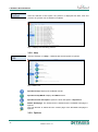
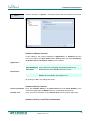
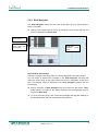
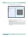
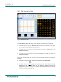
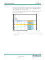
Content
User Manual
1
Software Version 1.0
Content
2
Software Version 1.0
Content
Content
1.
Overview........................................................................................................ 6
1.1.
What is SpotScout and SpotScout Pro .......................................................... 6
1.2.
System Requirements .................................................................................... 6
1.3.
Program Version ............................................................................................ 7
1.4.
Content and Structure of the Manual ............................................................. 7
1.5.
Writing Rules .................................................................................................. 7
1.6.
License Information ........................................................................................ 7
2.
Software Installation and Connection with MArS ..................................... 9
3.
Software Documentation ........................................................................... 11
3.1.
3.1.1.
3.1.2.
3.1.3.
3.1.4.
Program Structure and Operation ................................................................ 11
Structure of the Program Window ................................................................ 11
Operation ...................................................................................................... 12
Program Structure ........................................................................................ 17
File Formats.................................................................................................. 18
3.2.
3.2.1.
3.2.2.
3.2.3.
3.2.4.
3.2.5.
3.2.6.
3.2.7.
3.2.8.
3.2.9.
Menu File ...................................................................................................... 19
Save ............................................................................................................. 19
Save As ........................................................................................................ 20
Open ............................................................................................................. 21
Close ............................................................................................................ 21
Information.................................................................................................... 21
Recent .......................................................................................................... 21
LabBook ....................................................................................................... 21
Help .............................................................................................................. 22
Options ......................................................................................................... 22
3.3.
3.3.1.
3.3.2.
3.3.3.
3.3.4.
3.3.5.
3.3.6.
3.3.7.
Menu Viewer................................................................................................. 26
Overview....................................................................................................... 26
Slide Navigator ............................................................................................. 27
Area Navigator ............................................................................................. 28
Histogram ..................................................................................................... 28
Spot Viewer .................................................................................................. 29
Ribbon – View Functions .............................................................................. 29
Ribbon – Lookup Table Functions ............................................................... 30
3.4.
3.4.1.
3.4.2.
3.4.3.
3.4.4.
3.4.5.
3.4.6.
Menu Protocol .............................................................................................. 31
Overview....................................................................................................... 31
Protocol Flow ................................................................................................ 32
Section Save Options ................................................................................... 33
Define New Session ..................................................................................... 35
Load Protocols ............................................................................................. 35
Start/Stop the Processing of the Protocol .................................................... 37
3.5.
3.5.1.
3.5.2.
3.5.3.
3.5.4.
Menu Scan ................................................................................................... 38
Overview....................................................................................................... 38
View Functions ............................................................................................. 39
Scan Functions ............................................................................................. 39
Section Scan Settings .................................................................................. 40
3
Software Version 1.0
Content
3.5.5. Section Grid Structure .................................................................................. 41
3.6.
3.6.1.
3.6.2.
3.6.3.
3.6.4.
3.6.5.
3.6.6.
3.6.7.
3.6.8.
Menu Evaluation (only SpotScout Pro) ........................................................ 43
Tab Finding Settings .................................................................................... 44
Tab Quality Settings ..................................................................................... 45
Grid Finding Options .................................................................................... 47
Evaluation Options ....................................................................................... 48
Flags Visibility Options ................................................................................. 48
Tab Histogram .............................................................................................. 49
Tab Scatter Plot ............................................................................................ 50
Tab Evaluation Table ................................................................................... 51
4.
Appendix ..................................................................................................... 53
4.1.
Evaluation Table ........................................................................................... 53
4.2.
License Information ...................................................................................... 54
4
Software Version 1.0
Content
Dear customer
We are delighted that have chosen SpotScout or SpotScout Pro, a ScanSoftware to control the Microarray Scanner MArS of Ditabis and to qualify and
evaluate biochip image data.
The Software has been developed with utmost care involving the use of newest
tools and high-performance algorithms to allow routine operation as well as
individual research tasks.
The intuitive user navigation makes working with the SpotScout (Pro) very simple.
The operator’s manual includes all that you need for operating the software and for
using all implemented functions.
We wish you every success in solving your tasks with SpotScout (Pro). If you
have any questions or if a problem occurs, please do not hesitate to contact us.
Your Ditabis AG Development Team
Freiburger Straße 3
75179 Pforzheim
www.ditabis.de
5
Software Version 1.0
2. Software Installation and Connection with MArS1. Overview
1. Overview
1.1. What is SpotScout and SpotScout Pro
SpotScout is the basic module of the scanner software to control the MArS
Microarray Scanner and to display biochip image data for analysis. It is also
possible to load and display image data of other devices if they are available as 16
bit grey scale images in TIF format. Besides, it is possible to import all GAL files.
SpotScout Pro additionally includes the complete evaluation module to evaluate
image data automatically or pursuant to individual specifications:

Automatic grid finding

Quantification of image data

Reliable and efficient quality control (spot position evaluation, artifact
identification, saturation check) with report

Export of the results in GPR format
With the evaluation module of SpotScout Pro you can also evaluate TIF image
files.
Definition of Terms
To simplify matters, we talk about the software system SpotScout in this operator’s
manual if functions are concerned which exist in both systems. SpotScout Pro is
used if functions are concerned existing only in this system.
1.2. System Requirements
Hardware
Processor
2GHz (multi-core recommended)
Main Memory
at least 2GB (4GB recommended)
USB 1.0
Software
Operating System
Windows XP – Win7 (only 32bit!)
Acrobat 6.0 or higher
MArS with firmware 1.0.32 or higher
During a scan, no other software besides SpotScout may be running.
6
Software Version 1.0
1. Overview
1.3. Program Version
Version 1.
1.4. Content and Structure of the Manual
The available manual is the operating manual and software documentation for
SpotScout and SpotScout Pro. Since SpotScout is a subset of SpotScout Pro,
it is indicated which software functions surpass the basis module SpotScout.
Basically, it is the menu Evaluation.
The manual is structured in such a way that every user can immediately find “his”
parts.
Chapter 1
includes an overview over the software, explains the writing rules and provides
license information.
Chapter 2
describes the installation of the software and the connection with the Microarray
Scanner MArS as well as the activation of the Software with the license key.
Chapter 3
represents the Software documentation. Here, the individual functions and their
meaning are described.
Chapter 4
is the appendix with further explanations about the program.
1.5. Writing Rules
In the available manual we use the following writing rules for better orientation:
The names of Menus, Options, Register
Tabs etc. are written in bold letters
File, Viewer, Protocol
The Selection of an Option in a Menu is
written as a command sequence, separated
by a vertical line
File | Options
Buttons, if not depicted, are written in bold
letters and set in angle brackets
<Save>, <Open>, <Close>
Enumerations

Action steps

1.6. License Information
ZedGraph is published under LGPL
GNU LESSER GENERAL PUBLIC LICENSE
Version 3, 29 June 2007
7
Software Version 1.0
2. Software Installation and Connection with MArS1. Overview
Copyright (C) 2007 Free Software Foundation, Inc. http://fsf.org/
Please read the license information completely and observe it. It is included in the appendix
in chapter 4.2.
8
Software Version 1.0
2. Software Installation and Connection with MArS.
2. Software Installation and Connection with MArS
This chapter describes the installation of SpotScout or SpotScout Pro on your PC
and the connection of the PC with the Microarray Scanner MArS and the
activation of the Software.
You get the Software either on CD-ROM or by download.
After the Installation of the Software, the Software is activated by receiving a
license key from Ditabis AG.
Installation Procedure
 You get the Setup file on the enclosed CD-ROM or have downloaded it.
 Start the file setup.exe.
 When asked for the target drive,
C:\Programme\Ditabis\SpotScout\.
enter
the
desired
path,
e.g.
 If .Net Framework 4.0 is not installed on your computer it will be automatically
installed during the setup.
 If you connect the Microarray Scanner MArS with the PC for the first time you
have to install the corresponding USB driver:
 For that, switch on MArS, wait a few seconds and connect the instrument with
your PC with an USB cable.
 The PC now detects a new USB device and Windows requests you to search a
corresponding driver in a directory. Select the setup directory or the directory
you have downloaded. After that, the USB driver is installed automatically.
 As last installation step, click on <Next> or <Continue>. Finally, Windows
indicates that the installation has been successful.
 The setup routine creates a file in the Start menu and the icon
desktop.
on your
 For starting SpotScout or SpotScout Pro double-click the program icon on
your desktop.
9
Software Version 1.0
2. Software Installation and Connection with MArS1. Overview
Activation of the Software with a License Key - Procedure
 Select “GetSpotScoutID” in the start menu. Then, the file “HardwareID.txt” is
created on your desktop.
 Send the file “HardwareID.txt” per email to [email protected].
 After having paid the license fee, we will send you the license file immediately.
Otherwise, you get information on payment options.
 Copy the license file in the SpotScout program directory and start SpotScout.
10
Software Version 1.0
3. Software Documentation
3. Software Documentation
3.1. Program Structure and Operation
3.1.1. Structure of the Program Window
After the program start (click on the program icon on the desktop), SpotScout or
SpotScout Pro is loaded and the program with the start window is displayed. This
is the window of the menu Viewer with the display fields for the images still being
empty.
If MArS is not connected and switched on, all functions are deactivated.
Quick Access Bar
with user-defined
tools
Menu Bar
Splitter Bar
can be moved
randomly
Ribbon
tools corresponding
to the selected menu
Display Bar for slots
and loaded files
Slide View
display of the loaded/
scanned image
Setting and
Evaluation Section
Status Display
Progress Bar for the
selected Slot
Loading
Status
Global Progress
Bar
Fig. 1: Structure of the Program Window
In all program parts, the program window is structured similarly. Only in the menu
File there is no Slide View.
11
Software Version 1.0
3. Software Documentation
3.1.2. Operation
Quick Access
You can copy buttons and tools which you use frequently from the Ribbon into the
tool bar Quick Access. Then, they are additionally available in every menu. The
quick access can be configured pursuant to your individual needs. For that, the
Context Menu of the individual Buttons or Functional Groups (e.g. View or
Lookup Table) is available. The options of the Context Menu are related to the
clicked-on object.
The buttons can be removed from the Quick Access again by opening the
Context Menu of the Button or the Functional Group in Quick Access and
selecting the relevant option (e.g. Remove...).
The options of the context menu
Add to Quick Access Toolbar
Remove from Quick
Access Toolbar
Customize
Toolbar…
Quick
Copies the clicked- on function or function group
into the Quick Access Bar.
Reversing: Right mouse click on the function or
the functional group in the Quick Access Bar
and select Remove...
Access Via a dialogue window, selected functions of all
menus can be selected and copied in Quick
Access or removed from Quick Access.
Place Quick Access Toolbar Relocates Quick Access into the bar below or
below/ above the Ribbon
above the Ribbon.
Minimize the Ribbon
Maximize the Ribbon
Fades the ribbon out.
Reversing: Right mouse click on a function in
Quick Access opens the Context Menu with the
option Maximize the Ribbon.
Fig. 2: Context Menu of the functions on the ribbon
12
Software Version 1.0
3. Software Documentation
Procedure: Extend Quick Access (Option Quick Access Toolbar)
Copied into Quick Access
Fig. 3: Quick Access and Ribbon
 Click with the right mouse button on the desired function on the Ribbon. The
relating Context Menu (Fig. 2) is opened.
 Click on Add to Quick Access Toolbar. The relevant function is copied into
the Quick Access (Fig. 3).
Menu Bar
Here are the menus of the program. A click on the menu name activates the menu.
The tab of the active menu is highlighted brightly. The tab of the menu File is
always highlighted in orange.
Fig. 4: Menu Bar
Ribbon
Depending on the menu, the required functions and tools in the form of buttons are
arranged and subdivided into functional groups here. You can also move functions
which you use frequently to Quick Access. See above.
Setting and Evaluation Section
Depending on the menu, the parameters are entered or the displayed image can
be analyzed and evaluated here.
Display Bar for Slots and Loaded Files
Here, the four slot tabs as well as all loaded files are displayed. (A *.ses file always
only includes the files of one slot.) The active slot or the active file is highlighted.
By clicking on a slot or a file name, the relevant slot or file is activated.
A scan can only be performed in a slot tab. These tabs are always available if a
MArS is connected and identified.
13
Software Version 1.0
3. Software Documentation
The files can also be selected via the drop-down menu of the Display Bar <▼>.
The active file is closed via <x> in the Display Bar.
Slide Display
In this section, the scanned or loaded image is displayed. The following scroll and
zoom functions are available if the zoom function
is active:
Scroll vertically
Moving the mouse wheel
Scroll horizontally
Moving the mouse wheel with pushed <Shift> button
Enlarge/
reduce image
Moving the mouse wheel with pushed <Ctrl> button
Select
detail
and
zoom Draw a rectangle with the mouse. The selected detail is
zoomed to the size of the slide display.
Splitter Bar
The splitter bar between Slide Display and the Setting and Evaluation Section
can be moved randomly. For that purpose, the splitter bar is provided with a
marking in the middle to be dragged with the mouse or to be clicked on.
Move
Click on the marking of the splitter bar and move the
splitter bar in the desired direction with the mouse button
being pushed
Maximize
A click on the marking of the splitter bar enlarges the
image display to the total width of the program window
Restore
Double-clicking the marking of the splitter bar restores
the original division between the two sections. In the
maximized state, the splitter bar is on the far left at the
edge of the program window.
On the tabs Histogram and Scatter Plot in the menu Evaluation (only SpotScout
Pro), clicking on the Splitter Bar has the effect that the image display is faded out
in favor of the result display.
Status Display
Status display for the scanner as well as for the analyzing processes like <Find
Grid> and <Analyze>.
14
Software Version 1.0
3. Software Documentation
Progress Bar of the Selected Slot
It displays the progress of the current action (like e.g. scanning) in the active slot in
%.
Loading Status
Unloaded
The MArS loading table is moved out.
Empty
The MArS loading table is in scan position and contains no
slides (sample carriers).
Loaded
The MArS loading table is in scan position and includes one
slide in the displayed slot (sample carrier).
Barcode
If the barcode is read it replaces the loading status.
Global Progress Bar
Displays the progress of the processing of a protocol in % of the total time (see
menu Protocol).
Context Menu of the Slide View Main Window:
A click with the right mouse button on the Slide View opens the Context Menu
with the following functions:
Navigate Back
The program returns to the last navigation setting (e.g.
zoom setting)
Navigate Forward
Proceeds by one navigation setting
Zoom
Activates the zoom function
Hand
Activates the hand function
Zoom to Slide
Zooms to the complete slide
Zoom to Scan
Zooms to the complete scanned image
Keyboard Control
The program can also be controlled via the keyboard:
Pushing the <Alt> button indicates the letter to perform a function.
For the options of the drop-down menu, the letter which performs the option is
underlined.
Default Protocol
15
Software Version 1.0
3. Software Documentation
A default protocol for all parameter settings is implemented in the program which
the user can define according to his needs. It must only be observed that there is
only one single default file.
There are two basic possibilities for a modification of the default protocol:

Modification of individual parameter groups: Every parameter group in the
menus Scan and Evaluation has a drop-down menu Presets. Here, the
relevant parameter group can be saved in the default file. Thus, only the
relevant parameters are overwritten, the remaining data remain unaffected.

Modification of the complete default protocol is performed if you save a
protocol in the menu Protocol as default file, since then the associated
settings are saved together with the protocol steps.
As standard, the default file is loaded if a new session is opened (<New Scan
Sessions>).
Drop-Down Menus Presets
In the drop-down menus Presets there is the possibility to save the current settings
of the associated parameter group and to load or to delete settings already saved.
Save
Saves the parameter group under a user-defined name.
Save as Default
Saves the parameter group in the available default file (see
above).
Load Default
If you have overwritten a default file, you can restore the
previous state of the default file with this command.
Organize
Lists the available parameter files in this parameter group.
Here, you can delete files.
Import from
Session
Here, you can read in parameters of a session file. For that,
the available *.ses files are displayed.
Import GAL
This option is only available for grid settings. Here, a GAL file
with a grid structure can be loaded.
xxx
In the lower part of the window, the available presets of the
relevant parameter group are displayed.
16
Software Version 1.0
3. Software Documentation
3.1.3. Program Structure
The program is subdivided into several menus which refer to special program
functions:
Menu File
It includes

Functions for loading and saving of files,

Function for modifying program settings as well as

Information and documentation functions.
Menu Viewer
In the menu Viewer, the loaded or scanned images are displayed, in which you can
navigate, zoom and analyze spots with the different functions. A histogram shows the
color value distribution of the complete image.
Menu Protocol
In the menu Protocol, the steps for a session (from the parameter input to
scanning and evaluation) are defined as a Protocol Flow and the complete
process is started. The parameter input itself is done in the menus Scan and
Evaluation (only SpotScout Pro) or by loading saved protocols in the menu
protocol.
For routine analyses, protocols saved by means of Quick Function can be loaded
with corresponding scan and grid parameters and the scan and evaluation process
can be started.
Menu Scan
Here, the Scan Parameters as well as the Grid Structure for the slide (sample
carrier) are defined. A single slot can be scanned with the parameters defined
here or be tested with a Preview Function.
Menu Evaluation (only SpotScout Pro)
Before scanning, the Evaluation Parameters are defined in the evaluation menu.
After scanning, the image is analyzed and evaluated here. The results are
available as Result Table (GPR format). The values of the result table can be
directly assigned to every spot in the slide view. Besides, Regression Analyses
with random value pairs can be performed and displayed as Scatter Plot.
Additionally, a report on the quality of the evaluation can be created.
17
Software Version 1.0
3. Software Documentation
3.1.4. File Formats
SES Files
Files with the ending .ses are created by SpotScout. Here, all information,
program and scan settings as well as evaluation settings and results (only for
SpotScout Pro) are saved per slot. Additionally, the image files are saved as TIF
files – corresponding to the number of images and used filters. They have file
names which correspond to the associated *.ses file. When loading a *.ses file, the
associated TIF files are also loaded.
To prevent the destruction of the relationship of these files, you
should not modify the names of the files and copy all related files
when copying.
TIF Files
The scanned images are saved as *.ses files and associated TIF files. It is also
possible to load individual TIF files (16 bit grey scale images), even if they originate
from other scanners. In this case, SpotScout Pro only needs the information
included in the TIF file.
You can also save a session as TIF file. In this case, only image data are saved, all
other data get lost.
GAL Files
GAL files (GenePix® format) include grid definitions for slides. They can be directly
loaded in the menu Scan and replace a manual creation of the grid structure.
GPR Files
The results are given in GPR file format (GenePix® Format). They include image
data and analysis data. In this format, the evaluation results of SpotScout Pro are
given.
SEP and SLT Files
In this format, protocols are saved.
HTML Format
The reports of SpotScout Pro are saved in HTML format.
BAK Files in case of Computer Crash
In case of a computer/software crash, you are prompted to save the current
session. In case of an inconsistency of the new file, the previous session is saved
as backup (file extension *.bak).
18
Software Version 1.0
3. Software Documentation
3.2. Menu File
After the selection of the menu File, the menu window with the menu options (on
the left) and the option Recent (last used files and directories) is displayed (see
Fig. 5).
Fig. 5: Menu File with options and default setting Recent
3.2.1. Save
A click on <Save> saves the session or image file active in the menu Viewer.
If a *.tif file is active, the selection window Save as always appears at the function
<Save> to define the name and to select the file format. Loaded *.tif files can also
be saved as *.ses files. In this case, they also include the additional information of
the session.
If the opened file is a *.ses file, the available file is overwritten with the changes.
Default setting for the saving of file images is
My Files\MArS\ScanImages.
19
Software Version 1.0
3. Software Documentation
3.2.2. Save As
This option saves the session or image file active in the menu Viewer under a new
name to be entered.
The following settings have to be considered and made:
 Enter the desired File Name.
 Set the desired File Type (*.tif or *.ses). Please observe the explanations on
the file types in chapter 3.1.4.
 Set the desired memory mode:
Single TIFF:
Every scan image (e.g. per ScanSetting, per area) is
saved as individual *.tif file.
Multi TIFF:
All images are saved in a *.tif file.
Multi TIFF per Area: All images per area are saved in a *.tif file.
 Enter the desired Orientation of the image. For that, click on the arrow button
next to Orientation. A selection list opens where the orientation of the sample
carrier is pictorially represented.
Fig. 6: Dialogue window Save as
20
Software Version 1.0
3. Software Documentation
3.2.3. Open
The default path for the opening of image files is:
My Documents\MArS\ScanImages.
This path can be modified like in the Windows Explorer.
Open file:
 Select the desired path.
 Select the desired file type (*.ses; *.tif or *.*).
 Select the desired file name and click on <Open>.
3.2.4. Close
By clicking on <Close>, the file currently active in the menu Viewer is closed. If the
data have not yet been saved or if you have made modifications you are asked
whether you want to save the data.
3.2.5. Information
By clicking on <Information>, the program version of SpotScout or SpotScout
Pro is displayed.
3.2.6. Recent
By clicking on <Recent>, the documents (column Recent Documents) and
directories (column Recent Places) opened recently are displayed (see Fig. 5).
 If you click on a document in the column Recent Document, the relevant
image file is opened and displayed in the menu Viewer.
 If you click on a directory in the column Recent Places, here the relevant
directory with the files included therein is displayed. Here, you can select and
load a file. The file is displayed in the menu Viewer.
Permanent Display
The displayed files and directories are provided with one pin each, displayed as
loose pin
. By clicking on a pin, the file or the folder are displayed permanently
even if it has not been opened for a long time. This is marked symbolically by an
inserted pin
(see Fig. 5).
3.2.7. LabBook
In the LabBook, all processes of SpotScout are protocolled and saved.
21
Software Version 1.0
3. Software Documentation
After the selection of this option, the protocol is displayed with date, time and
process. No process can be deleted or modified.
Fig. 7: Display of a laboratory protocol
3.2.8. Help
After the selection of <Help>, a window with several options is opened.
Fig. 8: Menu File
SpotScout Help. Displays the available manual.
SpotScout Help MArS. Displays the MArS manual.
SpotScout short description. Opens the short description of SpotScout.
Ditabis Homepage. The web browser is started and the DITABIS homepage is
opened.
The web browser is started and the contact page of the DITABIS homepage is
opened.
3.2.9. Options
22
Software Version 1.0
3. Software Documentation
After the selection of <Options>, a dialogue window with two submenus is opened:
Fig. 9: Menu Options, submenu Options | General
Submenu Options | General
In this submenu, the general appearance (Appearance) of SpotScout and the
size of the spots in the Spot Viewer (Menu Viewer and in the menu Evaluation,
tab Scatter Plot and Evaluation Table) can be modified:
Appearance
Color scheme
Here, the color scheme can be selected (blue, black, silver)
Show brightness If the control box is activated, the brightness values are
near cursor
displayed in the menu Viewer next to the cursor.
Spot Viewer
Zoom
With the slider control, the spot size displayed in the Spot
Viewer can be modified. See chapter 3.3.5
By clicking on <Ok>, the settings are saved.
Submenu Device | General
Device Information Here, the Firmware Version, the FPGA Version and the Serial Number of the
scanner are displayed if the MArS Scanner is connected and switched on.
Preview scan
Here, the scanner resolution for the Preview Scan can be selected (spot size).
Submenu Device | Laser/Filter Combination
23
Software Version 1.0
3. Software Documentation
Fig. 10: The four preset laser/filter combinations
The four preset laser and filter combinations (see Fig. 10) are displayed.
Meaning of the individual columns:
Name
Name of the laser/filter combination.
Laser
The possible values (Red/Green) depend on the desired laser [Red
(635 nm) or Green (532 nm)].
Filter
Filter position on the filter wheel in MArS (see Fig. 11). Possible
values are 1...8.
CalCor
Calibration correction value. At the delivery of the device it is “0” =
no correction. For user-defined filter settings, a deviating value can
be entered here, which affects the value in the column Calibration.
Please note that the top value is 255 counts there.
Calibration
This is the calibration value individually identified for your device. It
can be between 0 and 255.
24
Software Version 1.0
3. Software Documentation
Add Individual Laser/Filter Settings
You can add any individual settings according to the arrangement of the filters in
the filter wheel of MArS.
Procedure
 Click on the <+> button. A new line is added to the available table.
 Enter the parameters of the additional filter pursuant to the above description.
 Confirm the entry by clicking on <Apply>.
 For more filters, repeat this process accordingly.
 To save the modifications, click on <Ok>.
4
5
6
3
2
8
1
Fig. 11: Filter wheel with the position numbers for the individual filters
Be careful when handling the setting of the calibration correction
factors: Even minor modifications of e.g. 1% can increase the
measured fluorescence measuring signal by 6 to 10 %.
25
Software Version 1.0
3. Software Documentation
3.3. Menu Viewer
The menu Viewer is the start page of the program as well as the display page for a
loaded file or a scanned slide.
The menu window is subdivided into the following sections:

Ribbon with all tools for image setting and navigation

Display bar for loaded files and slots

Setting and evaluation section with navigators, histogram and Spot Viewer

Slide View with display of the scanned or loaded image.
Ribbon
Display Bar for
loaded files and slots
Setting and
Evaluation Section
Slide View
Fig. 12: Menu Viewer, setting: slide - total view
3.3.1. Overview
Via the Slide Navigator and the Area Navigator, desired image details for the
Slide View can be selected and enlarged or reduced. Likewise, the Slide View
itself can be zoomed (see chapter 3.1.3). These settings mirror themselves in the
navigator windows and show you the image detail with surroundings (Area
Navigator) within the total view of the slide (Slide Navigator).
The Histogram shows the brightness distribution of the total image as well as the
number of counts at the cursor position in the image or in the section you have
highlighted in the histogram with the cursor.
The Spot Viewer indicates the spot and background values for the spots on which
the cursor is placed. A setting of the size of the indicated spots can be made in the
menu File | Options | General (3.2.9).
26
Software Version 1.0
3. Software Documentation
3.3.2. Slide Navigator
The Slide Navigator shows the total view of the slide, the grey frame shows a
block on the slide.
 Clicking on the block sets the zoom on the block in such a way that only the
block is indicated in the Slide View.
Blue Rectangle
Zoom range
Blue Rectangle
Zoom range with
surrounding
Slide View
zoomed
image
detail
Fig. 13: Selection in Slide Navigator and display in Slide View
Set and Move Zoom Range
The blue rectangle is the range which is currently displayed in the main window.
You can define a random blue rectangle in the Slide Navigator and with that
define the zoom range for the main window and move it afterwards. At the same
time, the selected range is displayed in the Area Navigator together with the
surrounding.
 Drag a rectangle in Slide Navigator with the mouse with the button <Strg>
being pushed. According to the drawn rectangle, the corresponding range is
zoomed in Slide View.
 To move the zoom range, click on the blue rectangle and drag the rectangle in
the desired direction with the mouse button being pushed.
27
Software Version 1.0
3. Software Documentation
3.3.3. Area Navigator
In addition to the selected image detail, the Area Navigator shows a range around
the displayed image detail (see Fig. 13).
Set and Move Zoom Range
 A random rectangle can be drawn with the mouse in the Area Navigator.
Accordingly, the display in Slide View changes.
 To draw a range within the blue frame, push the button <Strg> and draw the
desired rectangle with the button <Strg> being pushed.
 The “dragging” on one side of the frame enlarges or reduces the detail in the
main window.
 To move the zoom range, click on the blue rectangle and drag the rectangle in
the desired direction with the mouse button being pushed.
3.3.4. Histogram
The histogram illustrates the distribution of the color values of the complete image. In
order to visualize the distribution, the Y-axis is displayed logarithmically (default). You
can also change to linear illustration. Depending on the setting either the red or the
green or both channels (see chapter 3.3.7) are displayed at the same time (see Fig.
14). For the relevant cursor position, the corresponding values (Level, Red count,
Green count) are displayed numerically. A random range can be dragged with the
mouse. Thereby, the values for this range (Level from ... to; Red count; Green
count) are shown. The selected range is displayed in orange. If you push and hold
the button <Strg>, the percent values instead of the absolute values for the red
and/or green channel are displayed (see Fig. 14).
Fig. 14: Histogram illustration with selected range
The histogram also shows whether the scanned image is overexposed or
underexposed. If the values on the left side of the histogram are too high, the
image is underexposed, if peaks appear on the right side of the histogram, the
image is overexposed.
28
Software Version 1.0
3. Software Documentation
3.3.5. Spot Viewer
The Spot Viewer shows the extreme enlargement of the spot which is in Slide
View below the cursor. At the same time, the intensity value is displayed at the
cursor position. After evaluation, the brightness of the spot and the background for
every channel (Red Channel, Green Channel, Overlayed) is displayed. Below
there are the values for the X-Y-position of the cursor on the slide.
Abb. 15: Spot Viewer
3.3.6. Ribbon – View Functions
Goes to the previous or next view.
In this drop-down menu there are preset zoom factors. Next to these values, a
random zoom factor up to 10000% can be entered. The input must be confirmed
with <Enter>.
Those three functions are related to the scanned image:
The loaded image is enlarged until the width or the height of the scan
exactly fills in the main window.
The loaded image is enlarged until the scanned part is completely visible in
the main window.
Those three functions are related to the slide
The slide is displayed in full width or in full height.
In the main window, the zoom factor is set so that the slide is entirely visible.
Zoom tool. If this tool is activated, a section can be selected in the Slide View with
the mouse which then is enlarged accordingly (see chapter 3.1.2).
Hand tool. If this tool is active, the image can be moved in the Slide View so that
another image detail is displayed. For that, you have to click on the image and
drag it.
In the drop-down menu Orientation, the orientation of the slide can be changed
in steps of 90°.
29
Software Version 1.0
3. Software Documentation
With the option As saved, the image is displayed in the saved original position.
As saved
3.3.7. Ribbon – Lookup Table Functions
Selection of the displayed channel (red or green). In case of more than one scan
image, the desired image can be selected via a drop-down menu <▼>.
The selected images are overlaid (red and green channel).
In this drop-down menu, the type of the lookup table can be selected:
Brightness/Contrast, Ramp and False color.
Via the slider control (on the right), the parameters can be set. The relevant
setting is displayed on the screen. (As long as the slider control is hold with the
mouse, the image is displayed in the preview mode.) If the function Linked is
active, red and green are set via one slider control, otherwise via separate slider
controls.
Option Brightness/Contrast: Via the slider control, Brightness and Contrast of
the image can be set.
The option Ramp is the default setting. At Low, the lowest and at High, the
highest intensity value for the desired illustration is entered. Between those two
values, the illustration from black to bright (color) takes place. Values below the
low value are illustrated black, values above the high value are illustrated bright.
Option False color: The intensity values are shown on the color scale. See
explanations for the option Ramp.
Automatic setting of the LookUp Table.
If this function is active, the Lookup Table settings for all sessions are taken over.
If this option is active, the red and the green channel are set via joint slider
controls. Otherwise, different slider controls are displayed for the two channels.
30
Software Version 1.0
3. Software Documentation
3.4. Menu Protocol
Fig. 16: Menu Protocol: Protocol Flow in the left section, above: file name
3.4.1. Overview
Display of the defined steps in a Protocol Flow and Start
In the Protocol Flow, the steps to be processed are defined. The steps include the
settings which are made in the menus Scan and Evaluation (only SpotScout Pro)
for the active slot.
The steps highlighted in yellow are active and are performed. The individual steps
of the Protocol Flow are displayed as buttons which can be activated or
deactivated by clicking.
Next to the step switches, the scan surface and the settings of the active slot are
displayed like they are defined by the selected protocol.
Define New Session
Via the button <New Sessions>, new sessions in the four slots can be defined.
Then, the parameters for the new session can be entered by loading available
protocols or by entering the parameters for the currently active slot in the menus
Scan and Evaluation (only SpotScout Pro).
31
Software Version 1.0
3. Software Documentation
Saving the Session
In the section Save Options, the saving parameters for the session can be
defined.
Starting the Scan Process
With the defined settings, the scan process either for the active or for all occupied
and defined slots can be started via the button <Start>.
3.4.2. Protocol Flow
The meaning of the individual steps:
Read Barcode
Scans the barcode.
Scan Slide
Scans the loaded slots.
Find Grid
Searches the grid structure pursuant to the preset parameters
(only for SpotScout Pro).
Evaluate Spots
Performs the evaluation pursuant to the preset evaluation
parameters (only for SpotScout Pro).
Save Session
Saves the session under the file name specified in Save
Options.
Export Results
Exports the evaluation results as GPR file (GenePix® Results).
It is filed together with the session file under the same name.
The files only differ from each other in the ending.
Create Report
Creates a HTML report about the quality of the evaluated grid
structure. The report is filed together with the session file under
the same name. The files only differ from each other in the
ending.
32
Software Version 1.0
3. Software Documentation
3.4.3. Section Save Options
Fig. 17: Section Save Options
Here, it is specified how the scanned image is to be saved.
Please note that a *.ses file only includes the data of one slot each!
Mode
Selection of the file format in which the image (not the session)
is to be saved. Multi TIFF, Single TIFF and Multi TIFF per area
can be selected. See chapter 3.1.4.
Stitched Areas
If the checkbox is activated, the section between the areas is
filled black (intensity 0) and one single image is created per
Scan Setting.
Orientation
By clicking on the arrow button, the drop-down menu is opened
in which it is defined with which orientation the image is to be
saved.
Folder
Specification of the folder in which the file is to be filed. Default
setting is My Files\MArS\ScanImages\.
File Name
Specification of the file name. By clicking on the arrow button,
the dialogue window Auto Filename for the input of the
parameters for the file name opens (Fig. 18). After the saving
of the entries, the file name is displayed.
Fig. 18: Dialogue window Auto Filename
33
Software Version 1.0
3. Software Documentation
For the automatic scan process with the Protocol Flow, please note that the file
names are generated automatically. For the automatic naming, a selection of the
following elements in random order can be used:
<Date>, <Time>, <Barcode>, <Prompt> and <Fixed text>.
As separator, you can use either an underline or a blank.
Procedure
 Define the Separator.
 If you want to use a specified text in the file name, enter it in the box Fixed
Text.
 Then, click on the element buttons in the desired order. The selected elements
are then displayed in the box Order.
 To change the order, you can use the arrow buttons below the box Order
(explanation see below).
 To delete an element, click on <
>.
 By clicking on <OK> you save the parameters for the file name.
The Elements of the automatic file naming in detail:
Date
Uses the current date for the file name
Time
Uses the current time for the file name
Barcode
Uses the barcode for the file name. The barcode is read
before the Slide Scan
Prompt
Uses a Prompt for the file name. The Prompt can then be
specified before the processing of the protocol in a pop-up
window.
Fixed Text
You can add a fixed text which e.g. characterizes the
sample.
Moves the element highlighted in the box Order forward by one position.
Moves the element highlighted in the box Order backward by one position.
Deletes the highlighted element.
34
Software Version 1.0
3. Software Documentation
3.4.4. Define New Session
A new session for all slots is defined via the button <New Scan Sessions>.
 Click on <New Scan Sessions>. A possibly opened session is closed and a
new protocol for all slots is opened.
 If information of an old session which is not yet saved is available, a save
prompt is performed. If applicable, save the data of the last session. Only then,
a new protocol for all slots is opened.
A new session for the active slot is defined via the drop-down menu of the button
<New Scan Sessions>.
 Click on the drop-down menu of <New Scan Sessions> and then the option
Current Slot. A possibly opened session for the active slot is closed and a
new protocol for this slot is opened.
3.4.5. Load Protocols
In the ribbon, the protocol files already saved are displayed.
At the first program start, only placeholders for the protocols are displayed (Fig.
19). After the protocol has been saved, the placeholder is replaced as well as the
name of the saved protocol is displayed.
Fig. 19: Display of the placeholders for protocols in the ribbon
Fig. 20: Saved protocol
Save/Delete Protocol - Procedure
35
Software Version 1.0
3. Software Documentation
 Click on the arrow button in the protocol display (see red arrow in Fig. 19). The
drop-down menu with the available protocols as well as the options is
displayed.
 For saving, select the option Save and then enter the desired file name in
the dialogue window.
 You can also save a protocol as default protocol (Option Save as
Default). Since there is only one default file (Default), you are asked
whether you want to overwrite the previous settings in the default file. If
you confirm this, the old default file is overwritten with the new files (see
also the details on default files, page 15).
 To delete a protocol file, select the option Organize. The window
Organize Protocols opens in which all protocols are listed. Highlight the
protocols to be deleted and click on the button <Delete>.
Load Protocol – Procedure
 To load a protocol, click on the desired protocol in the ribbon. The highlighted
protocol is loaded for the active slot.
Quick Load Function
Via the button <Quick Load> a quick load function for protocols is available to
provide several slots with protocols subsequently.
Procedure
 Click on <Quick Load>. The quick load function is activated.
 Click on the desired protocol in the ribbon. Then, the selected protocol for the
active slot is loaded. At the same time, the program jumps to the next slot and
activates it.
 Click on the protocol that you want to assign to this slot. It is loaded and the
program jumps to the next slot.
 In this way, you can provide all slots one after the other with different (or
identical) protocols.
36
Software Version 1.0
3. Software Documentation
3.4.6. Start/Stop the Processing of the Protocol
The protocol can be started if the protocol steps and the saving parameters are
defined.
Start the Processing of the Protocol - Procedure
 To scan all slots, click on <Start>.
 To scan only the displayed slot, click on the drop-down menu of <Start> and
select the option Current Slot.
 Then, all steps of the Protocol Flow are processed automatically and – if
defined in the Protocol Flow - saved. The data are saved per slot in a *.ses
file.
Stop the Processing of the Protocol - Procedure
 Click on the button <Stop>. The processing of the protocol is stopped.
 To proceed with the processing, click on <Start> again or select the option
Start | Current Slot again in the drop-down menu of the button <Start>.
37
Software Version 1.0
3. Software Documentation
3.5. Menu Scan
Fig. 21: Menu Scan
3.5.1. Overview
Parameter Input and Grid Definition
In the left section, the parameters for the scanning and the grid structure of the
active slot are entered. The parameters can be saved via the corresponding dropdown menus Presets and saved parameters can be loaded.
In the slide view, the settings are displayed.
Scanning
The active slot can be scanned according to the entered settings: As preview (with
lower resolution) or as optimal scan. The barcode can also be scanned.
Please note that these scanning functions only refer to the active slot. In the menu
Protocol, all slots can be scanned one after the other automatically.
38
Software Version 1.0
3. Software Documentation
3.5.2. View Functions
If this button is active, the defined block structure is faded in as halftransparent image in the Slide View.
The range which is scanned at the moment is displayed.
3.5.3. Scan Functions
If MArS is closed, the loading table is retracted.
The barcode is scanned in the active slot.
The preview image of the current slide is generated in one or all
wavelengths for the active slot with low resolution. The selection can be
selected via the related drop-down menu.
Scans the active slot with current settings.
Stops the current scan process.
39
Software Version 1.0
3. Software Documentation
3.5.4. Section Scan Settings
Fig. 22: Scan Settings
The scan parameters for the active slot are displayed. In our example, it is Slot 3.
These parameters can be saved via the button <Presets> or available parameters
can be loaded.
The Parameters in Detail:
Displays the resolution (spot size) in µm with which the slide is scanned.
Selection of the laser and filter for the scan process.
Intensity of the laser with which the slide is scanned.
Data transfer via the standard channel
Data transfer via the high channel
Data transfer in Dual Mode, St and Hi
Allows adding more wavelengths.
Removes the currently selected wavelength.
Moves the selected wavelength in the scan sequence down by one position.
Moves the selected wavelength in the scan sequence up by one position.
Setting possibility of the Defocus in µm.
Loading / saving of the settings for the scan process. See page 16.
40
Software Version 1.0
3. Software Documentation
3.5.5. Section Grid Structure
Here, the grid structure and the distances between the blocks are defined.
Fig. 23: Grid Structure and Barcode Settings
The Parameters in Detail
Number of Blocks
Number of blocks in X – or Y – direction.
Block Size
Size of blocks
First Block Location
X and Y position of the first block
Block Spacing
Distance between the individual blocks.
Scan Overrun
Indicates the scan excess, i.e. how far does the scanner
scan beyond the block borders. Tolerances of spotter and
insertion tolerances are evened out.
Block Naming
Naming of the blocks. You can select numerical or
alphabetical for each the X – or Y – coordinate.
Number of Spots
Number of spots within a blocks in X – and Y – direction.
Barcode Settings
Size
Indication of the size of the barcode
Location
Indication of the position of the barcode
Type / Orientation
Selection of barcode type and orientation
Presets
Loading / saving of the grid structure settings (see details
on Presets on page 16).
Hints for the Setting of the Grid Structure
41
Software Version 1.0
3. Software Documentation
 First define the top left block.
 For that, measure the size of this block and enter the values in the line Block
Size.
 Then measure the position of this block on the slide and enter the values in the
line First Block Location.
 Measure the distance between the blocks and enter the value in the line Block
Spacing.
 Enter the number of blocks in X- and Y-direction in the line Number of Blocks.
42
Software Version 1.0
3. Software Documentation
3.6. Menu Evaluation (only SpotScout Pro)
Fig. 24: Evaluation Ribbon: Finding Settings
The menu Evaluation is provided with two different functionalities:

Parameter input for evaluation. For that, 2 tabs in the left section are available
(Finding Settings, Quality Settings).

Evaluation after the scan process: Display of the used parameters and display
of the evaluation results. For that, more tabs are available in the left section
(Histogram, Scatter Plot and Evaluation Table). After evaluation, the
parameters for the Grid Finding can be changed as well as specific evaluation
and analyzing functions can be performed which are available in the form of
buttons in the ribbon.
43
Software Version 1.0
3. Software Documentation
3.6.1. Tab Finding Settings
Parameters for the Finding of the Grid Structure (see Fig. 24).
Auto Shift Limit
Here, the maximum distance of the ideal grid structure
is defined within which spots are still searched. 100%
corresponds to half the spot distance.
Spot Cutting
Fraction
This parameter defines the lower intensity limit. It
defines how much background is to be deducted of
each spot in percent.
Radius Detection
This parameter defines whether the grid finding is to be
performed with a fix or variable radius.
Radius Interval
This parameter defines the range for the spots radii,
which is acceptable. 100% corresponds to the radius of
the spot.
Spot Eccentricity
Maximum
Here, the possible eccentricity of the expected spots,
i.e. the deviation from an exact circle is set. A value of
0% means that only perfect circles are accepted as
spots. A value of 10% means that also slightly oval
spots are accepted. At the maximum input of 100%,
even a linear spot is accepted.
Rotation Angle
Maximum
Here, the angle is entered by which the grid can be
maximally rotated. The smaller the angle entered here,
the smaller the searching range of the grid finding
function.
Low Signal
Enhancement
This parameter influences the depth of focus for lower
image signals. High image signals lead to an exact
analysis while lower values consume storage space
and evaluation time in favor of a high-grade detection
of lower spot signals.
Presets
Via the drop-down menu, Grid Finding parameters
can be saved or saved parameters can be loaded. See
details on Presets on page 16.
44
Software Version 1.0
3. Software Documentation
3.6.2. Tab Quality Settings
Fig. 25: Tab Quality Settings
Section Evaluation Settings
Good Shaped Spot
Radius Interval
With these parameters, the upper and lower limit for
the deviation of a spot position from the defined
position is set. The distance is entered as
percentage of the spot radius median. Values of
more than 100% are possible.
Saturated Spot
Area Threshold
This parameter defines the limit from which a spot is
considered to be overexposed. Here, the
percentage of spot pixel is entered which has an
intensity value of more than 98% of the maximum
intensity.
45
Software Version 1.0
3. Software Documentation
Section Array Quality Settings
Here, the limits for the evaluation ranges are defined. They are the basis for the
Report.
In the medium range, values are accepted as OK (“Green”).
This range is followed at both ends by ranges with the evaluation “yellow”. Outside
those ranges, the evaluation is „red“.
Fig. 26: Scheme Quality Parameter
For the levels as well as for the following parameters, a weight for flowing
into the total evaluation and the definition as exclusion criteria can be made.
The exclusion criteria say: if the parameter concerned delivers a red
evaluation, the chip must be evaluated as being red.
Average Signal
Limits for the average intensity of all spots.
Signal Variance
Limits for the variance of the intensity of all spots.
Image Saturation
Limits for the percentage
overexposure limit.
Average
Background
Limits for the average background intensity of all spots.
Saturated Spots
Limits for the percentage of overexposed spots within the
relevant spot range.
Poorly-Sized
Spots
Limits for the percentage of badly positioned spots within the
spot range.
No-Signal Spots
Limits for the percentage of no-signal spots within the spot
range.
User tagged
Limits for the percentage of user-defined spots within the
spot range
Presets
Loading or saving of parameters. See details on Presets on
page 16.
46
Software Version 1.0
of
the
pixels
above
the
3. Software Documentation
3.6.3. Grid Finding Options
In this section of the ribbon, the options for Grid Finding are summarized.
Starts the Grid Finding. For that, at least 5 spots must be defined.
By another click on this button, the function is reset. By yet another click, the grid
finding is started again.
Cancels the Grid Finding.
Activates the tool Move Spot. Then, click on the button <Spot> or <Block>. By
that, you can move a spot or a spot block or all spots (with the mouse button being
pushed).
If you select a range with the button <Strg> being pushed, the spots in this range
are highlighted and the spots in this range which have already been highlighted
remain highlighted.
Tool to move a spot. The tool Move Spots must be activated.
Tool to move a spot block. The tool Move Spots must be activated.
Tool to move all spots together. The tool Move Spots must be activated.
Resets the last spot movement.
Repeats the last spot movement.
47
Software Version 1.0
3. Software Documentation
3.6.4. Evaluation Options
In this section of the ribbon, the evaluation options are summarized.
Analyzes the spots within a grid structure.
Cancels the grid analysis.
To be able to evaluate the data with other programs, the analyzing result can be
exported as *.gpr file (gene pix results).
Creates a HTML Report which describes the quality of the grid analysis. The report
is filed together with the session file of the same name.
Tool to highlight spots. Individual spots are highlighted by clicking. A spot group is
highlighted by selecting the relevant range with the mouse. If you push the button
<Strg> during that, spots already highlighted in this range remain highlighted.
3.6.5. Flags Visibility Options
In this section of the ribbon, the options are summarized with which the flags
defined by the evaluation parameters can be displayed.
Display of the highlighting symbols for the spots highlighted by the user. See
tab Quality Settings, parameter User tagged.
Display of the highlighting symbols for the spots classified as “bad”. See tab
Quality Settings, parameter Poorly-sized Spots.
Display of the highlighting symbols for the spots classified as no-signal spots.
See tab Quality Settings, parameter No-Signal Spots.
Display of the highlighting symbols for the spots classified as saturated. See
tab Quality Settings, parameter Saturated Spots.
48
Software Version 1.0
3. Software Documentation
3.6.6. Tab Histogram
Fig. 27: Evaluation Ribbon: Histogram
Please read description in chapter 3.3.4.
49
Software Version 1.0
3. Software Documentation
3.6.7. Tab Scatter Plot
After the analysis of the spots, two new tabs are displayed in the left section,
Scatter Plot and EvaluationTable.
Fig. 28: Tab Scatter Plot with an example evaluation
In Scatter Plot, all features of the spots, like e.g. background intensity of the
relevant wavelength can be plotted against each other on the X-axis and on the Yaxis.
The blue line in the plot is a Regression Line, which is calculated depending on the
selected value pairs.
The symbol size of the displayed spots can be set in the box Symbol Size below
the Scatter Plot. By clicking on <Default Scale>, the original size is restored.
When you move the mouse over a spot, the ID of the spot is faded in via Tooltip
and the relevant spot is displayed in the Spot Viewer.
50
Software Version 1.0
3. Software Documentation
3.6.8. Tab Evaluation Table
Fig. 29: Evaluation Table
In the Evaluation Table, all results of the analysis of the slide are summarized.
 A double-click on a spot in Slide View lets the table jump directly to this spot,
e.g. in Fig. 29, spot 5396 has been clicked on.
 A double-click on a spot in the table positions the spot in Slide View in the
middle of the image.
 A double-click on the splitter bar between Slide View and Table (see page 14)
maximizes the table.
Next to the vertical splitter bar, there are two other splitter bars above and below
the table:
 A double-click on the lower splitter bar hides/shows the Spot Viewer.
 A double-click on the top splitter bar opens/closes the section where columns
displayed in the evaluation table can be selected. Selected columns are
highlighted by ticks. Clicking on a checkbox deactivates/activates the relevant
column in the table (see Fig. 30).
51
Software Version 1.0
3. Software Documentation
In Fig. 30, the columns ID, X and Y are faded out. Likewise, the column Name of
spot 5396 has been changed into an example text. In the Evaluation Table, the
columns Name, ID can be individually labeled.
The columns User Tag, No Signal, Poor Size and Saturated can also be
changed via drop-down menu.
Fig. 30: Evaluation Table with edited names
If you move over the lines with the cursor in the table, the relevant spot is displayed
in the Spot Viewer.
52
Software Version 1.0
4. Appendix
4. Appendix
4.1. Evaluation Table
Block
Column
Row
Name
ID
X
Y
Dia
Columns created by the evaluation algorithms:
Block number of the feature
Column number of the feature (in block)
Row of the feature (in block)
Description field for spot
Description field for spot
X-coordinate in μm of the center of the feature-indicator associated with the
feature, where (0,0) is the top left of the image
Y-coordinate in μm of the center of the feature-indicator associated with the
feature, where (0,0) is the top left of the image
Diameter in μm of the feature indicator
For each analyzed channel (XXX marks channels wavelength):
FXXX Median
FXXX Mean
median feature pixel intensity
mean feature pixel intensity
FXXX SD
standard deviation of the feature pixel intensity
FXXX CV
Coefficient of variation - is calculated by FXXX SD/ F XXX Median
BXXX
median feature background intensity
BXXX Median
median feature background intensity
BXXX Mean
mean feature background intensity
BXXX SD
standard deviation of the feature background intensity
BXXX CV
Coefficient of variation - is calculated by BXXX SD/ B XXX Median
%>BXXX+1SD
percentage of feature pixels with intensities more than one standard
deviation above the background pixel intensity
%>BXXX+2SD
percentage of feature pixels with intensities more than two standard
deviations above the background pixel intensity
FXXX%Sat.
FXXX Median –
BXXX
FXXX Mean – BXXX
Percentage of feature pixels which intensity equals the maximum intensity
the median feature pixel intensity at wavelength with the median
background subtracted
the mean feature pixel intensity at wavelength with the median background
subtracted
FXXX Total
Intensity
SNR XXX
the sum of spot pixel intensities at wavelength Index number of the spot as
it occurs on the array
the signal-to-noise ratio at wavelength, defined by (Mean Foreground 1 –
Mean Background 1)/(Standard deviation of Background 1)
53
Software Version 1.0
4. Appendix
4.2. License Information
ZedGraph is published under LGPL
GNU LESSER GENERAL PUBLIC LICENSE
Version 3, 29 June 2007
Copyright (C) 2007 Free Software Foundation, Inc. http://fsf.org/
Everyone is permitted to copy and distribute verbatim copies of this license document, but
changing it is not allowed.
This version of the GNU Lesser General Public License incorporates the terms and
conditions of version 3 of the GNU General Public License, supplemented by the additional
permissions listed below.
0. Additional Definitions.
As used herein, "this License" refers to version 3 of the GNU Lesser General Public License,
and the "GNU GPL" refers to version 3 of the GNU General Public License.
"The Library" refers to a covered work governed by this License, other than an Application or
a Combined Work as defined below.
An "Application" is any work that makes use of an interface provided by the Library, but
which is not otherwise based on the Library.
Defining a subclass of a class defined by the Library is deemed a mode of using an interface
provided by the Library.
A "Combined Work" is a work produced by combining or linking an Application with the
Library. The particular version of the Library with which the Combined Work was made is
also called the "LinkedVersion".
The "Minimal Corresponding Source" for a Combined Work means the Corresponding
Source for the Combined Work, excluding any source code for portions of the Combined
Work that, considered in isolation, are based on the Application, and not on the Linked
Version.
The "Corresponding Application Code" for a Combined Work means the object code and/or
source code for the Application, including any data and utility programs needed for
reproducing the Combined Work from the Application, but excluding the System Libraries of
the Combined Work.
1. Exception to Section 3 of the GNU GPL.
You may convey a covered work under sections 3 and 4 of this License without being bound
by section 3 of the GNU GPL.
2. Conveying Modified Versions.
If you modify a copy of the Library, and, in your modifications, a facility refers to a function or
data to be supplied by an Application that uses the facility (other than as an argument
passed when the facility is invoked), then you may convey a copy of the modified version:
a) under this License, provided that you make a good faith effort to
ensure that, in the
event an Application does not supply the function or data, the facility still operates, and
performs whatever part of its purpose remains meaningful, or
54
Software Version 1.0
4. Appendix
b) under the GNU GPL, with none of the additional permissions of this License applicable
to that copy.
3. Object Code Incorporating Material from Library Header Files.
The object code form of an Application may incorporate material from a header file that is
part of the Library. You may convey such object code under terms of your choice, provided
that, if the incorporated material is not limited to numerical parameters, data structure
layouts and accessories, or small macros, inline functions and templates(ten or fewer lines
in length), you do both of the following:
a) Give prominent notice with each copy of the object code that the Library is used in it and
that the Library and its use are covered by this License.
b) Accompany the object code with a copy of the GNU GPL and this license document.
4. Combined Works.
You may convey a Combined Work under terms of your choice that, taken together,
effectively do not restrict modification of the portions of the Library contained in the
Combined Work and reverse engineering for debugging such modifications, if you also do
each of the following:
a) Give prominent notice with each copy of the Combined Work that the Library is used in it
and that the Library and its use are covered by this License.
b) Accompany the Combined Work with a copy of the GNU GPL and this license document.
c) For a Combined Work that displays copyright notices during execution, include the
copyright notice for the Library among these notices, as well as a reference directing the
user to the copies of the GNU GPL and this license document.
d) Do one of the following:
0) Convey the Minimal Corresponding Source under the terms of this License, and
the Corresponding Application Code in a form suitable for, and under terms that
permit, the user to recombine or relink the Application with a modified version of the
Linked Version to produce a modified Combined Work, in the manner specified by
section 6 of the GNU GPL for conveying Corresponding Source.
1) Use a suitable shared library mechanism for linking with the Library. A suitable
mechanism is one that (a) uses at run time a copy of the Library already present on
the user's computer system, and (b) will operate properly with a modified version of
the Library that is interface-compatible with the Linked Version.
e) Provide Installation Information, but only if you would otherwise be required to provide
such information under section 6 of the GNU GPL, and only to the extent that such
information is necessary to install and execute a modified version of the Combined Work
produced by recombining or relinking the Application with a modified version of the Linked
Version. (If you use option 4d0, the Installation Information must accompany the Minimal
Corresponding Source and Corresponding Application Code. If you use option 4d1, you
must provide the Installation Information in the manner specified by section 6 of the GNU
GPL for conveying Corresponding Source.)
55
Software Version 1.0
4. Appendix
5. Combined Libraries.
You may place library facilities that are a work based on the Library side by side in a single
library together with other library facilities that are not Applications and are not covered by
this License, and convey such a combined library under terms of your choice, if you do both
of the following:
a) Accompany the combined library with a copy of the same work based on the Library,
uncombined with any other library facilities, conveyed under the terms of this License.
b) Give prominent notice with the combined library that part of it is a work based on the
Library, and explaining where to find the accompanying uncombined form of the same work.
6. Revised Versions of the GNU Lesser General Public License.
The Free Software Foundation may publish revised and/or new versions of the GNU Lesser
General Public License from time to time. Such new versions will be similar in spirit to the
present version, but may differ in detail to address new problems or concerns.
Each version is given a distinguishing version number. If the Library as you received it
specifies that a certain numbered version of the GNU Lesser General Public License "or any
later version” applies to it, you have the option of following the terms and conditions either of
that published version or of any later version published by the Free Software Foundation. If
the Library as you received it does not specify a version number of the GNU Lesser General
Public License, you may choose any version of the GNU Lesser General Public License
ever published by the Free Software Foundation.
If the Library as you received it specifies that a proxy can decide whether future versions of
the GNU Lesser General Public License shall apply, that proxy's public statement of
acceptance of any version is permanent authorization for you to choose that version for the
Library.
56
Software Version 1.0