1
objsegm
– User Manual
D. Schlesinger, TU Dresden
September 4, 2007
Contents
1
Introduction
2
2
Theoretical background
3
3
Overview
3.1 Elements . . . . . . . . . . . . . . . . . . . . . . . . . . . . . . . . . .
3.2 Building of a complex model . . . . . . . . . . . . . . . . . . . . . . . .
6
6
7
4
Detailed description
4.1 Options, common for all elements . . . .
4.2 Feature maps . . . . . . . . . . . . . . .
4.3 Parameters . . . . . . . . . . . . . . . . .
4.4 Options, common for all models . . . . .
4.5 Options, common for terminal models . .
4.6 Options, common for non-terminal models
4.7 Model overview . . . . . . . . . . . . . .
4.7.1 Non-terminal models . . . . . . .
4.7.2 Terminal models . . . . . . . . .
5
Interface
5.1 Setting the options . . . . . . . . . . .
5.1.1 Models . . . . . . . . . . . . .
5.1.2 Feature maps . . . . . . . . . .
5.1.3 Adding the learning information
5.2 Output . . . . . . . . . . . . . . . . . .
5.2.1 Text-output . . . . . . . . . . .
1
.
.
.
.
.
.
.
.
.
.
.
.
.
.
.
.
.
.
.
.
.
.
.
.
.
.
.
.
.
.
.
.
.
.
.
.
.
.
.
.
.
.
.
.
.
.
.
.
.
.
.
.
.
.
.
.
.
.
.
.
.
.
.
.
.
.
.
.
.
.
.
.
.
.
.
.
.
.
.
.
.
.
.
.
.
.
.
.
.
.
.
.
.
.
.
.
.
.
.
.
.
.
.
.
.
.
.
.
.
.
.
.
.
.
.
.
.
.
.
.
.
.
.
.
.
.
.
.
.
.
.
.
.
.
.
.
.
.
.
.
.
.
.
.
.
.
.
.
.
.
.
.
.
.
.
.
.
.
.
.
.
.
.
.
.
.
.
.
.
.
.
.
.
.
.
.
.
.
.
.
.
.
.
.
.
.
.
.
.
.
.
.
.
.
.
.
.
.
.
.
.
.
.
.
.
.
.
.
.
.
.
.
.
.
.
.
.
.
.
.
.
.
.
.
.
.
.
.
.
.
.
.
.
.
.
.
.
.
.
.
.
.
.
.
.
.
.
.
.
.
.
.
.
.
.
8
9
9
10
10
11
12
12
12
13
.
.
.
.
.
.
19
19
19
19
20
20
21
5.2.2 Image-output . . . . . . . . . . . . . . . . . . . . . . . . . . . .
Error messages . . . . . . . . . . . . . . . . . . . . . . . . . . . . . . .
21
22
6
Examples
6.1 Program objsegm_simple . . . . . . . . . . . . . . . . . . . . . . .
6.2 Segmentation examples . . . . . . . . . . . . . . . . . . . . . . . . . . .
23
23
26
7
Conclusion
32
8
Acknowledgments
38
5.3
1
Introduction
This is the user manual for the software system objsegm. It it developed to perform
different kinds of segmentation. Usually the segmentation is considered as a dividing the
set of image pixels into disjoint subsets or, equivalently, as an assignment of a segment
name (number or label) to each pixel of the image. In doing so it is assumed, that the
pixels, which belong to a particular segment, are in a certain sense “similar”. The pixels,
which belong to different segments, are thereby “different”. In addition some prior knowledge about the segmentation itself should be often taken into account – e.g. compactness,
expected shape of segment boundaries etc. Depending on the chosen dissimilarity measure, different kinds of segmentation can be distinguished – e.g. threshold methods, texture
segmentation etc. However, we would like to point out, that the segmentation itself is initially defined without any respect to some dissimilarity measure. The aim of the system
objsegm is not to perform some particular kind of segmentation, but rather to allow the
user to build and to apply different complex segmentation models based on some relatively
small number of “base models”.
This document is not an “user manual” in a usual sense, but rather something between
an “user manual” and a “programmers manual”. The reason for that is, that in case of
segmentation (to be able to use the system) it is absolutely necessary to understand not
only, what the system does, but also how does it work.
Technically the system is implemented as a library. The software package consists
of a couple of precompiled libraries (compiled under Linux with gcc 4.1.2), header
files and a simple program objsegm_simple, which illustrates the usage of the system
(is given as source code). We used Qt4 library by Trolltech. To compile the program
objsegm_simple, do the following:
– Download objsegm_<arch>.tgz, where <arch> is your architecture,
– Unpack it e.g. by tar -xzf objsegm_<arch>.tgz,
– Go to the directory objsegm_<arch>/objsegm_simple,
– Run qmake-qt4 followed by make
If all went right the executable objsegm_simple occurs in the current directory.
The rest of the user manual is organized as follows:
– In the next section we recall briefly the theoretical background of our approach.
– In section 3 an overview of system parts will be given (in 3.1) as well as an explanation, how a complex segmentation model can be built using base models (in
3.2).
– Section 4 contains the detailed description of system elements.
– In section 5 the interface part of the system will be explained – how to set parameters, visualize the results etc.
– Finally we give in section 6 examples, which illustrate the usage of the system and
the program objsegm_simple.
2
Theoretical background
In this section we recall briefly the theoretical background, which our approach is based
on. More detailed considerations can be found e.g. in the following sources:
– Labeling problems: [8, 13, 2, 4, 11];
– Gibbs Sampler: [6, 9];
– Expectation-Maximization algorithm: [14, 1];
– Applications: [3, 5, 7, 10, 12].
Our approach is based on statistical modeling by Gibbs probability distributions. Let
us consider this in a little bit more detail on an example of a very simple segmentation
model. Let R be the set of pixels of an image and K be the set of segments (labels).
The segmentation is then a mapping f : R → K, that assigns a label from K to each
pixel r ∈ R of the image. In statistical modelling the a-priori probability distribution of
segmentations is often assumed to be a Gibbs probability distribution of second order:
Y
p(f ) ∼
grr0 f (r), f (r0 ) .
(1)
rr0 ∈E
Here E ⊂ R × R is the set of pairs of pixels, which are defined to be neighbors (we use in
particular the 4-neighborhood); f (r) ∈ K denotes the label, chosen by the segmentation
f in a node r ∈ R; functions g : K × K → R+ are quality functions, which mirror
assumptions for the a-priori probability distribution of segmentations (for instance the
Potts model with g(k, k 0 ) = exp[a · 1I(k = k 0 )]1 is suitable for segmentation tasks).
Let the conditional probability distribution for observations given a labeling be conditionally independent, i.e.
Y
qr f (r), x(r) ,
(2)
p(x | f ) =
r∈R
where x : R → X is the mapping, which maps the set of pixels into the set X of color
values, i.e. the image, functions q : K × X → R+ are local conditional probability
distributions p(x | k) to observe color value x given a label k.
The segmentation task can be posed in such models as a Bayes decision task with
respect to a cost function C(f, f 0 ) as follows:
X
f ∗ = arg min
p(f 0 | x) · C(f, f 0 ).
(3)
f
f0
Using of the additive delta cost function
C(f, f 0 ) =
X
1I f (r) 6= f 0 (r)
(4)
r∈R
leads to the following decision strategy:
f ∗ (r) = arg max p f (r) = k | x , where
k∈K
X
p(f, x)
p f (r) = k | x ∼
(5)
(6)
f :f (r)=k
Unfortunately there are no known
closed solutions to compute the marginal probability
distributions p f (r) = k | x . Therefore we use Gibbs Sampler to estimate these probabilities approximately.
1
1I(expr) = 1 if expr is true and 0 otherwise.
Besides of technical problems (approximate solutions), there are also many modeling
problems. First of all, simple observation models like (2) do not allow to model segments
adequately, if the appearances of the segments are complex themselves (e.g. if one segment is a texture). To overcome this difficulty it is often necessary to extend the label
set K by something in addition to take into account the look of each particular segment
(see e.g. [12]). Consequently the (less or more) general segmentation model (1) becomes
dependent on a particular application.
Let us consider briefly a technical aspect, namely the implementation of the Gibbs
Sampler for a simple segmentation model (1) and (2). To perform the generation by the
Gibbs Sampler it is necessary to calculate in a pixel r the following “local” conditional
probability distribution:
Y
pr (k) ∼ qr k, x(r) ·
grr0 k, f (r0 ) .
(7)
r0 :rr0 ∈E
It is easy to see, that it is thereby not necessary “to know”
the observation x, it is only
necessary to know the values of the function qr k, x(r) at the position r for all segments
k. Let us imagine, that each segment k ∈ K is represented in the implementation by
a “black box”, that gives the values of qr depending (somehow) on the actual position
r and the observed image x. Then the generation according to (7) could be obviously
performed. The Gibbs Sampler does not need to know even the types of the used segments
– conditionally independent probability distributions of grayvalues, textures, Gaussians
or whatever. The types of segments can be even different. Moreover, one “black box”
can be a segmentation model (like (1)) itself. It allows to connect segmentation models
hierarchically, building a tree-like structure of models.
The main idea of the system objsegm is the exploration of the fact, described above.
The system consists of a relatively small number of “base models”. Each model is able
to give for all pixels of the processed image values, which can be interpreted as probabilities of observation in these pixels. Segmentation models use these values to perform
segmentation, taking into account in addition their a-priori probability distribution of segmentations.
Another topic, that should be necessarily taken into account, is the following. Each
base model has (sometimes many) free parameters. When building a complex model from
the base ones, the number of free parameters in the whole model becomes very large.
Consequently there should be a possibility to learn them either in superwised or in unsupervised manner. We use mainly Expectation-Maximization schemes (derived for each
particular base model) to do that.
One of very important modeling problems is the fact, that in the scope of labeling
formulation it is very difficult to use prior knowledge about the form of segments. This
Elements
Models
Interface
Feature maps
Learning
information
Parameters:
Circles
Non-terminal models:
Split
SplitR
Modalities
Weight
Terminal models:
Background
Mix
Shading
General
Gshading
Texture
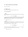
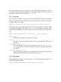
Figure 1: Hierarchy of elements.
is the case, because as a rule such information can not be incorporated into the model
“in a local manner”. To overcome this problem, some mechanism should be defined, that
allows “to influent segmentation model non-locally”. In our approach one such method is
realized. It is based on the assumption, that such non-local additional information can be
in principle seen as an unknown parameter of the probability distribution. The estimation
of this unknown parameter can be then performed according for instance to the Maximum
Likelihood principle.
3
Overview
3.1
Elements
In this subsection we give an overview of the parts of the system objsegm. We call these
parts “elements”. The classification/hierarchy of elements is illustrated in fig. 1. The most
essential part of the system consists of base models. They are divided into two groups.
– Non-terminal models (or shortly non-terminals) perform different types
of segmentations as well as some other kinds of “linking together” for other models.
– Terminal models (or shortly terminals) correspond to different types of
segments.
Each model performs its own kind of optimization. For some of them a generation procedure is necessary to estimate statistics, needed to perform optimization steps (for example
in a (1)-like segmentation model Gibbs Sampler should take place to estimate marginal
probabilities). Summarizing, the optimization/generation algorithm for each model consists of an infinite loop, so that in each iteration some activities are performed (e.g. one
optimization step). We call such a type of optimization/generation procedure “working
loop”.
Parameters represent non-local prior information for segmentation models. We
decided to define parameters as a separate element to realize a certain flexibility of the
whole system – one segmentation model can use many parameters, a particular type of
parameters can be used for different models etc. The behavior of parameters is similar
to the behavior of models – they have their own optimization procedure (working loop),
which consists of an infinite loop of optimization iterations.
Feature maps (or shortly maps) are responsible for loading of the input images
and performing of some preprocessing steps (e.g. convertion, normalizing etc.). Since
these elements do preprocessing only, they have no working loop – i.e. all activities are
performed before the working loops of the used models/parameters start.
Learning information is a static data block, which should be specified manually (if present) in advance. It allows to fix segments at some places of the processed
image. We will distinguish in further the learning information from other elements, because this information can not be seen as a part of a complex model. It is rather “an
additional input” for the system (like the input images). Therefore we will use in further
the notation “element” having in mind all parts of the system (presented in fig. 1) besides
of the learning information.
Interface is a system for storing and visualization of the results. It provides a
feedback only, i.e. it does not influent the behavior of the system.
3.2
Building of a complex model
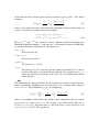
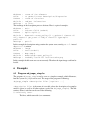
A complex model is a tree-like structure, where the leafs are terminal models and interior
nodes are non-terminal ones. The connections between elements in a complex model are
illustrated in fig. 2 .
– Each non-terminal model has children, which may be either terminals or non-terminals.
A non-terminal model has access to all its children as well as to its parent.
Non-terminal
Interface
Learning
information
Terminal
Parameter
Terminal
Non-terminal
Terminal
Map
Map
Figure 2: Complex model.
– Non-terminals may have parameters. Models have access to their parameters. Parameters have access to the models, to which they are attached.
– Non-terminal models may have an associated block of learning information.
– Each terminal model refers to exactly one feature map. Many terminals can refer to
one map. Terminals have access to their parents.
– Interface object is attached to the root of the model tree. Each model has its interface
functions. The interface object can call all interface functions of the model tree.
4
Detailed description
In this section we give a detailed description of elements. The majority of elements have
their options. Thereby some of them are common for all (or for a certain subset) of elements. Other are specific ones. At this place we would like to note, that the system
objsegm is still under development. We think, that at this stage it is much more important to specify the connections between the elements, rather then to fully implement
certain models. In this situation it is common, that not all elements, implemented so far,
fully support all options, which are foreseen yet. Let us suppose, that there is an option,
which is intended to be common for a certain subset of elements. But may be not for all
elements from this subset this option is relevant. In spite of this situation we would like to
present options as they are at the moment, apart from whether they are supported/used by
particular elements or not.
We prefer to describe firstly the options themselves. In doing so we will follow the
hierarchy of the elements (see fig. 1). After that we explain, how to set the options for
each particular element of a complex model.
The majority of options have less or more reasonable default values. They will be
given together with the corresponding options in form
<option>=<default value>.
4.1
Options, common for all elements
Name
Each element should be named. Name is a symbol string without empty spaces.
Names provide a way to identify elements, therefore they should be unique (otherwise the behavior of the system is unpredictable). At the moment this option is
not relevant for Interface, because it need not be identified/accessed by other
elements of the system. Interface obtains a “dummy” default name. For all
other elements this option is mandatory.
reset_policy=31
Each element can be reset once awhile during the work. One reason for that could
be for example a program, that segments a sequence of images rather then a single
image (in particular this option is not used in the program objsegm_simple).
This option is a bitwise mask, which controls the behavior of the element, when
resetting. Each element interprets this option in its own way. At the moment this
option is supported by SplitR, Shading, Gshading and Circles.
4.2
Feature maps
They represent features, which are computed from input images in advance. Basically one
feature is a real number. The feature map is an array of real values, that has the same sizes
as the image. Their options are:
File
The filename of the image, from which the feature should be computed. Mandatory.
code=0
This options defines, which feature should be computed. At the moment the
following possibilities are realized:
0 features are graylevels of the image pixels,
1 features are taken from the red channel,
2 features are taken from the green channel,
3 features are taken from the blue channel,
4 experimental (images are stored in a special format).
align=-1.
If not equal −1, the values of the feature map are shifted to have the mean value
equal align.
4.3
Parameters
In contrast to models, which are less or more general, parameters are specific for each
particular application. So far we have implemented only one type of such non-local parameter, namely Circles. Therefore at the moment we have no specification of options
for this element.
4.4
Options, common for all models
Type
This option determines, which model is used. Should be one of the following:
Split, SplitR, Modalities, Weight, Background, Mix, Shading,
Gshading, General, Texture. Mandatory option.
Parent
This defines the name of the parent for the model in a complex model. If it is not
given, the object is assumed to be a root of the model tree.
The following three options control the behavior of the working loop. One iteration of the
loop consists of successive calls of the following procedure:
1. Perform optimization/generation step,
2. Once per n_update iterations perform an update step,
3. Adjust timeout,
4. Wait timeout milliseconds.
All working loops of the whole complex model work in parallel (technically, objsegm
is realized as a multithreaded system). Each working loop performs a kind of indirect
synchronization by adjustment of its timeout (time to sleep). The adjustment procedure
follows the principle: “The number of iterations performed by me so far should be similar
to the number of iterations performed so far by my parent”. timeout of the root remains
constant.
n_update=0
This option controls, how often an update-procedure is called during the working
loop. The default value 0 means “never”. Such an update-procedure is implemented yet only for Split, General and Texture. Thereby it has almost
no influence in Split and General (the default situation “never update” is
suitable in most cases). The update-procedure of Texture in contrast contains
a learning step. Therefore the default value causes situation, that the texture parameters are not learned at all. Obviously it is only reasonable, if the used texture
is pre-learned in advance (see Texture description for details).
timeout=10
This option sets the initial timeout for the working loop.
min_timeout=1
This option sets the lower limit for the timeout of the working loop.
4.5
Options, common for terminal models
Map
Each terminal model should refer to exactly one Map. This option sets the name
of the map, which the model refers to. It is mandatory.
4.6
Options, common for non-terminal models
There are no such options.
4.7
Model overview
In this subsection a more detailed description of models is given.
4.7.1
Non-terminal models
Split
This model performs segmentation according to the Potts model. It means, that the quality
function grr0 in (1) is
a if k = k 0
0
g(k, k ) =
(8)
1 otherwise
(position independent). The model uses the Gibbs Sampler to estimate marginal a-posteriori
probabilities of labels in each pixel. The decision for each pixel is done according to (5).
At the moment this model does not support parameters. The only one option is
potts=10.
Potts parameter a in (8).
SplitR
This is an extention of the Potts model. The state set K is supposed to be ordered, i.e. states
are enumerated from 1 to |K|. The functions grr are just the same as for the model “Split”
except that jumps greater then 1 are disabled in addition:
a if k = k 0
0
1 if |k − k 0 | = 1
g(k, k ) =
(9)
0 otherwise.
At the moment this model dos not support the learning information. It supports
parameters. Just as in the previous case there is only one option
potts=10.
Potts parameter a in (9).
Modalities
This is a “transitional” model, which is used to combine many conditional probability
distributions to one under the assumption, that the original distributions are conditionally
independent. The model performs nothing other, but multiplication of probabilities, given
by its children:
Y
p x(r) | f (r) =
pi x(r) | f (r) ,
(10)
i
where i is the index for children models. This Model has no options. One iteration of the
working loop consists of simply recalculation of probability values for all pixels according
to (10).
Weight
This model is used to compute a weighted sum of probabilities, given by its children:
X
p x(r) | f (r) =
wi · pi x(r) | f (r) ,
(11)
i
P
where i is the index for children models, the weights wi satisfy wi ≥ 0, i wi = 1. A
simple example for this model is the Gaussian mixture – the children are Gaussians in
that case. The weights wi are learned during the working loop. The new values of wi
are computed as a convex combination of the old ones and the “best ones”, which are
estimated by an EM-like schema:
(new)
wi
(old)
= wi
(best)
· (1 − γ) + wi
· γ,
(12)
i.e. a step in the gradient ascent direction is performed. The options are:
step=0.1
The speed of learning, i.e. γ in (12).
w(<i>)=1.
Initial values for wi . The index <i> can vary from 0 to n−1, where n is the number of children models. After all parameters are set, the weights are normalized
to sum to 1.
4.7.2
Terminal models
Background
This terminal model realizes the Gaussian probability distribution for features. Let x(r)
be the value of the used feature (stored in the associated Map) in a pixel r. This model
computes
"
2 #
x(r) − µ
1
p x(r) = √
,
(13)
exp −
2σ 2
2πσ
where µ is the mean value and σ is the dispersion. During the working loop the values of
µ and σ are learned in a gradient ascent way as follows:
µ(new) = µ(old) · (1 − γ) + µ(best) · γ
σ (new) = σ (old) · (1 − γ) + σ (best) · γ · λ
(14)
Here are µ(best) and σ (best) the “actual best” values, which are estimated according to the
Maximum Likelihood principle, γ is the step size, λ is an heuristic parameter, which allow
to control the behavior of the dispersion. The options are:
mean=128.
The initial value of µ.
sigma=1000.
The initial value for 2σ 2 .
step=0.1
The step size, i.e. γ in (14).
l_q=1.
The value of λ in (14). As already said, this option is an heuristic one, i.e. the use
of other values than 1 is theoretically not grounded. For example use of λ > 1
causes the dispertion to be greater, as the “real” one. Use other then the default
values with care.
Mix
This model realizes a Gaussian mixture. It is in a certain sense obsolete, because the same
family of probability distributions can be realized by Weight together with a couple of
Backgrounds. The probabilities p x(r) are computed by
"
2 #
n
X
x(r) − µi
1
exp −
,
(15)
p x(r) =
wi · √
2
2σ
2πσ
i
i
i=1
where n is the number of Gaussians in the mixture, other notations have the same meaning as in Weight and Background. The weights wi are learned in the same way as
in Weight, i.e. by (12), the mean values µi and dispersions σi in the same way as in
Background, i.e. by (14). The options are:
ng=2
The number of Gaussians in the mixture.
step=0.1
The step size γ.
m(<i>)=128.
The initial mean value µi for the i-th Gaussian. The index <i> vary from 0 to
n − 1.
s(<i>)=1000.
The initial value of 2σi2 for the i-th Gaussian.
w(<i>)=1.
The initial weight wi for the i-th Gaussian. After all options are set, the weights
are normalized to sum to 1.
l(<i>)=1.
The parameter λi for the i-th Gaussian.
General
This model realizes a general discrete probability distribution p(x). The values of the
feature x (stored in the associated Map) are thereby rounded to the closest integer value
and cut to the range 0 to 255 (initially, this model was designed to represent probability
distributions of grayvalues). Speaking shortly, the probability distribution is represented
by an array of 256 real values, one per one value of x – i.e. the normalized histogram. This
histogram is learned during the work by a gradient ascent method, i.e. one iteration of the
working loop consists in the recalculation
p(x)(new) = p(x)(old) · (1 − γ) + p(x)(best) · γ,
(16)
for x = 0 . . . 255, where p(x)(best) are the “best” values, which are estimated according to
Maximum Likelihood principle. This model has only one option
step=0.1
The step size γ in (16).
Shading
This model assumes, that there is an “ideal” field of feature values, where the values
in two neighboring pixels (according to the 4-neighborhood) differ not more, then some
predefined constant. This unknown “ideal profile” of feature values is considered as a field
of hidden variables and modelled by the following Gibbs probability distribution. Let us
denote by c : R → Z the field of hidden variables, let as usual x : R → R denote values,
stored in the associated Map. The probability of a pair (c, x) is
Y
Y
p(c, x) ∼
g c(r), c(r0 ) ·
q x(r), c(r) ,
rr0 ∈E
where
0
(17)
r∈R
g(c, c ) =
1
0
if |c − c0 | ≤ δ
otherwise.
(18)
In this model the Gaussian is used for q:
q(x, c) = p(x|c) = √
h (c − x)2 i
1
.
exp −
2σ 2
2πσ
(19)
One iteration of the working loop consists of a generation step for the field c (one iteration
of the Gibbs Sampler), followed by the learning step for σ. The latter is learned in a
gradient ascent way similar to (14). The options of this model are:
init_mode=0
Controls the initialization of the field c. Possible values are:
0 All values c(r) are set to mean (see below).
1 The initial field c is chosen in such a way, that it satisfies the conditions (18)
and “fits good” (in some reasonable sense) the whole associated feature
map – i.e. the model assumes, that it is visible everywhere.
mean=128
The initial value for c(r) if init_mode=0, if init_mode=1 this option is
ignored.
sigma=1000.
The initial value for 2σ 2 .
min_sigma=10.
The lower bound for 2σ 2 .
l_q=1.
The parameter λ, which is used to control the behavior of the dispersion during
the learning (see (14)).
jump=1
The maximal difference of values in two neighboring pisels – i.e. δ in (18).
step=0.1
Step size λ in (14).
Gshading
This model is a kind of superposition of General and Shading. As in the Shading
there is an unknown slowly varied field c, which represents “value shift”. The conditional
probability distribution q(x, c) is in contrast not the Gaussian, but a general probability
distribution of the “shifted” value (x − c). Summarized, the model is
Y
Y
p(c, x) =
g c(r), c(r0 ) ·
q x(r) − c(r) ,
(20)
rr0 ∈E
r∈R
where the function g(c, c0 ) is just the same, as in Shading, i.e. (18), function q(x, c) =
p(x − c) is a general probability distribution. During the working loop fields c are generated according to the a-posteriori probability distribution p(c|x) by the Gibbs Sampler.
The probability distribution q is learned using Expectation Maximization algorithm in an
gradient ascent way (like in (16)). It is easy to see, that the Maximum Likelihood formulation is ambiguous, when learning/generating both c and q without further restriction.
Therefore the field c is normalized after each M-step to have the mean value equal zero.
The field c is initialized with constant zero value, the probability distribution q as uniform
probability distribution. The options are:
jump=1
The parameter δ in (18).
step=0.01
The step size γ in (16).
Texture
This model is a realization of ideas, given in [12]. This model is rather complex, therefore
we omit here a detailed description. The main idea is, that the texture can be represented by
a “template”, which can be understood an “elementary texture element”. A textured image
(or a textured segment) is characterized by a spatial distribution of templates over the field
of view. The template itself is a set of elements, which are organized in an orthogonal grid
(like pixels in an image). To each element a Gaussian probability distribution of grayvalues
is attached, i.e. each element is characterized by its mean greyvalue and dispersion. The
options of this model are:
height_e=16
The height of the texture template.
width_e=16
The width of the texture template.
s_g=4.
The above mentioned distribution of templates over the field of view is modeled
by a Gibbs probability distribution of second order. This parameter controls,
“how regular” should be this distribution. Small values (about 1.) correspond to
very regular textures, big values (s_g≈height_e or width_e) correspond
to a weak regularity. For s_g→ ∞ the model nears to the simple mixture of
Gaussians with equal weights.
l_q=1.
The parameters of the template elements (mean values and dispersions) are
learned during the working loop in an unsupervised manner. Note, that the learning step for this model is performed by a special function, which is called once per
n_update iterations of the working loop. The option l_q controls the behavior
of dispersions (similar to (14)).
init_min=50
The mean values of the template elements are initialized randomly and uniformly
in the range init_min to init_max.
init_max=200
See above.
min_sigma=1.
The lover bound for the dispersions of the template elements.
step=0.01
Step size for learning of the template elements (for both mean grayvalues and
dispersions), similar to (14).
This model has its own “shading” part, which allow the mean grayvalues to (slowly) vary
over the field of view. The optimization of the shading part is performed in each iteration
of the working loop pixelwise as follows. In a pixel r the new value of shading is calculated
as a convex combination of the following components:
– The value, that fits as best as possible the feature value (stored in the associated
Map) at the position r;
– The actual shading value;
– The shading values of neighboring pixels.
The following three options are coefficients of this convex combination. After these options are set, they are normalized to sum to 1.
shad_next=1.
The more, the faster the shading converges.
shad_prev=100.
The more, the slower the shading converges.
shad_neigh=1000.
The more, the smoother is the shading profile.
5
5.1
5.1.1
Interface
Setting the options
Models
Technically the options are transferred to the models by passing a string, which describes
the passed options according to the following simple syntax:
<option>:<value> [<option>:<value> ...]
The string consists of fields, each one describing one option. The fields are separated by
empty spaces. The order of fields can be arbitrary. <option> is the name of the option,
described by this field (e.g. n_update, l_q, Type etc.). <value> is the value of the
option, which can be either a number or a string. There are some examples:
Name:segm1 Type:Split Parent:root potts:3
This string describes the non-terminal model of the type Split named segm1, whose
parent model (in the model tree) has the name root. The Potts parameter a in (8) is set
to 3. All other options are set to defaults.
Type:Background Parent:segm Name:b1 mean:100 Map:image
This string describes the terminal model of the type Background named b1, whose
parent model has the name segm. The initial mean value µ in (13) is set to 100. This
model refers to the feature map named image. All other options are default.
5.1.2
Feature maps
The feature maps are described in a similar manner, i.e. by a string like
Type:Map <option>:<value> [<option>:<value> ...]
(the key field Type:Map is used to distinguish Maps from models). There is an example:
Type:Map Name:red File:something.png code:1
This string describes the feature map named red, which stores the values from the red
channel (determined by code:1) of the image something.png.
Name:segm Type:Split ...
Name:s1 Parent:segm Type:Background ...
Name:s2 Parent:segm Type:Background ...
Learn:s1 0 0 34 51
Learn:s1 0 100 21 132
Learn:s2 200 58 220 70
Figure 3: Example – how to define learning information.
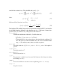
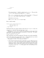
5.1.3
Adding the learning information
As already mentioned, each non-terminal model can have a block of learning information,
which gives the possibility to fix segments in particular pixels. This block consists of
elements, each one describing a rectangular area of the processed image, where a segment
should be fixed. One such rectangle is set by passing to a model of a string of type:
Learn:<child_name> <x_left> <y_top> <x_right> <y_bottom>
<child_name> is the name of a child model, whose label should be fixed. <x_...>
and <y_...> are the rectangle coordinates. In fig. 3 an example is given. It describes a
segmentation (model segm) into two segments called s1 and s2, which are Gaussians.
There are three rectangular areas, where the segments should be fixed – two rectangles for
the segment s1 and one for the segment s2.
– It is assumed, that x_left≤x_right and y_top≤y_bottom holds. Otherwise
the rectangle is empty.
– Segments are fixed inside the corresponding rectangles inclusive borders. For example a rectangle with x_left=x_right and y_top=y_bottom is just a single
pixel.
– If rectangle coordinates lay out of the image, this rectangle is cropped.
– If there are pixels, which are covered by many learning rectangles, the last occurring
<child_name> is used to fix segment in these pixels.
5.2
Output
As already mentioned there is an Interface object, which is a tool for storing and
visualization of the results. At the moment it provides a feedback only, i.e. it does not
allow interactions between the user and the system. Technically, the output is described
by a couple of strings, each one defining one “elementary” output. There are two types of
“elementary” outputs, that are managed by Interface.
5.2.1
Text-output
One elementary text-output is a string (we will call it output-string), which contains option
values for a particular model. Each model forms this string in its own way, depending on
its options. Here is an example:
Name:main timeout:40 gen_count:98 nobj:2 nlearn:2 potts:5
Some fields of the output-string describe options of the model, other are variables, which
are usefull for debugging. For instance gen_count is the number of iterations of the
working loop, performed so far. One elementary text-output is defined by a string as follows:
Output:Text Name:<name> [File:<file>] [Format:<format>]
Output:Text
The key field to identify an elementary text-output.
<name>
The name of the model, which should provide the output-string. This field is
mandatory.
<file>=out_<name>.log
This is the file name, where the string should be stored. If <file> is cerr
or cout the string is sent to the standart error stream or standart output stream
respectively.
<format>=<empty string>
This is the comma separated list of options/variables, which the output-string
should contain. If this field is absent, all options are given.
5.2.2
Image-output
Each model provides images to visualize results. One elementary image-output is described by a string like follows:
Output:Image Name:<name> code:<code> File:<file>
Output:Image
The key field to identify an elementary image-output.
<name>
The name of the model, which should provide the image. Mandatory.
<code>=1
The number, which identifies, what for image should be retrieved. Allowed numbers are: 1, 2, 3, −1 and −2. Each model interprets the code in its own way.
Thereby not all codes are supported by all models. The table below summarizes,
which codes are supported by which models at the moment:
1
Split
+
SplitR
?
Modalities ?
Weight
Background Mix
General
Shading
+
Gshading
+
Texture
+
2
+
+
3
?
+
? means, that a modell supports this code only, if there is no models of type
General in its subtree. The codes −1 and −2 are supported by all models but
they are mainly for debugging purposes.
<file>=out_<name>_<code>.png
The file name to store the image. The image format is always png (does not
depend on the extention).
5.3
Error messages
Since the interactions with user are not allowed yet, there is practically no other way to
handle errors, than simply to abort the program. In that case an error description is printed
out in the following format:
ObjName : <name of the element>
error
: <a general error description/diagnostic>
FnName : <name of function>
ObjInfo : <object information>
Message : <a hint>
The meanings of the description parts are obvious. Here is a pair of examples:
ObjName : main
error
: Unknown field (code=4)
FnName : Split::Split()
ObjInfo : Name:main reset_policy:31 n_update:0 timeout:40
min_timeout:1 gen_count:0 nobj:2 nlearn:2 Type:Split
potts:10
Message : pott:5.
In this example the description string contains the syntax error, namely pott:5. instead
of potts:5. is written.
ObjName : image
error
: Load (code=2)
FnName : Map::Map()
ObjInfo : Name:image reset_policy:31
Message : Probably could not load tentacke.png
In this example the file name was set not correctly. Therefore the input image could not be
loaded.
6
6.1
Examples
Program objsegm_simple
The program objsegm_simple can be seen as a simplest example, which illustrates,
how the system objsegm can be used. The usage of the program is following:
objsegm_simple <description file> [<option> ...]
<description file> is the name of a text file, where the description of a complex
model is given (as well as all other options, needed for objsegm_simple). This file
consists of lines, each line can be one of the following:
# <arbitrary text>
The lines, which start with # are comments.
END
The lines, following this one are ignored. They can be used e.g. to store some old
experiments, comments, notations etc. The line END is not mandatory, i.e. the
description file is processed until the end of file if there is no such string.
<model/interface/map/parameter/learning string>
The description string for a model (an elementary output, feature map, parameter,
learning item correspondingly). They describe element options according to the
format given in section 4.
<objsegm_simple option>
The program objsegm_simple has its own options (which do not relate to the
model tree). These are
Time=-1
The time to work in seconds. The default value “−1” means infinity. The
string, describing this option looks like
Time:<number>
dtime=10
The “output” activities of the Interface object are performed once
per each dtime seconds. The description string is
dtime:<number>
The order of lines is arbitrary. Each line can start or end with empty spaces, the fields
in a line can be separated by multiple spaces (the parser of objsegm_simple removes
unnecessary spaces). For convenience, the description file can be simplified in addition
in the following way to avoid repetitions of option values, which are common for many
elements. The following substitution is allowed. A couple of lines, which have common
parts, i.e. which look like
<prefix> <line 1> <suffix>
<prefix> <line 2> <suffix>
...
<prefix> <line n> <suffix>
can be replaced by
<prefix> {
<line 1>
<line 2>
...
<line n>
} <suffix>
– The opening bracket “{” should be attached to the <prefix>. The part of the
<prefix>-line, which is located right to the “{”, is ignored.
– The <suffix> should be in the same line as the closing bracket “}”. The part of
the <suffix>-line, which is located left to the “}” is ignored.
– Indentation is not necessary.
– Both <prefix> and <suffix> may be empty.
Here is a simple example:
Parent:main Type:Background {
Name:b1 mean:100
Name:b2 mean:150
} Map:image
This block describes two segments, which are of the same type Background, have common parent main and refer to the same feature map image.
The program objsegm_simple realizes also a possibility to transfer options by the
commandline. It is very usefull to perform experiments in a batch mode. The options,
given in the commandline have format
<name>:<option>:<value>
They override those, given in the description file. The options, given in the commandline,
can be model options or the program options only, i.e. neither options for Maps nor for
Interface nor learning information nor Parameter options.
The program objsegm_simple proceeds as follows:
1. First of all the description file and the commandline are parsed. Thereby the parser
of objsegm_simple does not check the syntax completely. It only makes substitutions (see above), merges together options from the description file and the
commandline options (if any) and separates lines by the element types (models,
Parameters, Maps etc.) – i.e. it only prepares lines for transferring to corresponding elements.
2. Then Maps are constructed (input images are loaded, preprocessing activities are
performed etc.).
3. The next step is the construction of the model tree. At this stage all description lines
are transferred to the corresponding models and Parameters. The majority of
errors occur just here because in this phase each model parses its options.
4. The Interface object is constructed. Thereby the description lines are not parsed
but only transferred to the Interface.
5. The working loops of all models in the model tree are started. Once per dtime
seconds the output activities of the Interface object are performed. If the description lines for the Interface were not correct, the error occurs.
6.
– If Time=-1 the working loops never stop, i.e. the program should be aborted
from outside.
– Otherwise the program finishes after Time seconds are elapsed.
6.2
Segmentation examples
In this section we give examples, which illustrate the usage of the system and in particular
the program objsegm_simple. Before we present the examples we would like to note
the following.
As already said our approach is based on statistical modeling. Moreover, most of the
used algorithms are mainly not deterministic, but stochastic ones (e.g. the Gibbs Sampler).
It means, that the results can be in principle seen as statistical variables itself. Therefore
they are in general not fully reproducible – they only “look similar”. Summarized, many
calls of the program may produce different results. Main source of this irreproducibility are random initialization of almost all components (in particular all segmentations are
initialized randomly if there is no learning information, associated with them). Another
source is the use of the Expectation-Maximization algorithm for learning. As known, it
does not converge in general to the global optima. Consequently “a reasonable” initialization of learned parameters is very usefull to make the results reproducible.
For each presented example we give the corresponding description files, used by the
program objsegm_simple. Among other things there are many parameters/options,
which influent “convergence speed” of the method (mainly the step option) as well as
the synchronization of model parts (e.g. timeout-s). In some cases these options influent
not only the speed of convergence but the results as well. We performed our experiments
mainly on a two processors computer with AMD64 X2. Consequently all options are
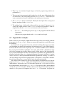
Figure 4: Artificial example – original image.
tuned to reach good results/reproducibility just on this computer. Eventually they should
be changed accordingly if working on other platforms.
The parameter Time in presented examples is set to a relatively big number to ensure
a segmentation, which is “the best one in scope of the used model”. As a rule, reasonable
results occur much earlier. In addition the time of generation can be essentially reduced,
if the learning of unknown parameters starts from a good initialization.
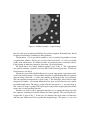
We begin with a very simple artificial example, given in fig. 4. The segmentation
was painted manually, segments were then filled with constant grayvalues. Finally the
Gaussian noise was added.
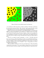
Obviously it is possible to build different (less or more) appropriate segmentation models for such a kind of images. One possibility would be to segment them into four segments
each one being a Gaussian – i.e. in the same manner, as the image in fig. 4 was produced.
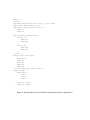
The corresponding description file is given in fig. 5. The Gaussians were learned in fully
unsupervised manner – no learning information was given and all Gaussians were initialized with default values. The images, produced by the root model main are given in fig. 6.
The “denoised” image is produced by replacing in each pixel the original grayvalue by the
mean value of corresponding Gaussian.
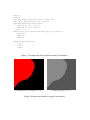
Another way (may be not so appropriate but faster) is to segment the image into only
two segments, assuming a Gaussian mixtures for both segments. The corresponding description file is given in fig. 7. In this case we initialized the mean values of Gaussians
with true ones (which were used to produce the original image). The option step is set to
Time:1000
dtime:2
Type:Map Name:image File:test5_20.png code:0
Type:Split Name:main potts:15 timeout:0
Type:Background Map:image Parent:main {
Name:b1
Name:b2
Name:b3
Name:b4
} step:0.1
Output:Text File:cerr {
Name:main
Name:b1
Name:b2
Name:b3
Name:b4
} Format:Name,gen_count,timeout,mean,sigma
Output:Image Name:main {
code:1
code:2
code:3
}
Figure 5: Description file for the artificial example (four Gaussians).
(a) Segmentation into four segments (code:2)
(b) “Denoised” image (code:3)
Figure 6: Results for the artificial example (four Gaussians).
a very small value, which corresponds to “almost no learning”. The images, produced by
the root model are presented in fig. 8. The “denoised” image contains grayvalues, which
are the weightet sum of mean values of Gaussians from corresponding mixtures.
Finally, the same scene can be modeled in an hierarchical manner: it consists of two
segments, each one consisting itself of two segments. The terminal models are Gaussian.
The corresponding description file is presented in the fig. 9. In that case it was also possible
to learn Gaussians in fully unsupervised manner without to violate the reproducibility (up
to the permutation of segments). The images, produced by the non-terminal models are
given in fig. 10. The “denoised” image is not shown since it looks very similar to that in
fig. 6.
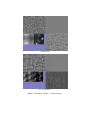
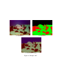
The next is an example of texture segmentation – see fig. 11. We should admit, that
here it was necessary to tune the parameters of textures very carefully. But with this parameters the segmentation were done in fully unsupervised manner (inclusive the learning
of texture templates). The corresponding description file is given in fig. 12. In fig. 13
the images, produced by the Texture models t1 and t2 are presented (see [12] for
description of image contents).
The last example is an image of a real scene, presented in fig. 14. The corresponding
description file is given in fig. 15. It is a good example to illustrate how to take into account
colors (in contrast to the above examples, where the input images were grayvalued ones).
Time:1000
dtime:2
Type:Map Name:image File:test5_20.png code:0
Type:Split Name:main potts:20 timeout:0
Type:Mix Map:image Parent:main {
Name:m1 m(0):50 m(1):200
Name:m2 m(0):150 m(1):100
} step:0.001
Output:Text File:cerr Format:Name,gen_count,timeout {
Name:main
Name:m1
Name:m2
}
Output:Image Name:main {
code:1
code:2
code:3
}
Figure 7: Description file for the artificial example (two mixtures).
(a) Segmentation into two segments (code:2)
(b) “Denoised” image (code:3)
Figure 8: Results for the artificial example (two mixtures).
Time:6000
dtime:2
Type:Map Name:image File:test5_20.png code:0
Type:Split Name:main potts:20
Type:Split Parent:main potts:10 {
Name:s1
Name:s2
}
Type:Background Map:image {
Parent:s1 {
Name:b1
Name:b2
}
Parent:s2 {
Name:b3
Name:b4
}
} step:0.1
Output:Text File:cerr {
Name:main
Name:b1
Name:b2
Name:b3
Name:b4
} Format:Name,gen_count,timeout
Output:Image {
Name:main {
code:1
code:2
code:3
}
Name:s1 code:2
Name:s2 code:2
}
Figure 9: Description file for the artificial example (hierarchical segmentation).
(a) Name:main code:2
(b) Name:s1 code:2
(c) Name:s2 code:2
Figure 10: Results for the artificial example (hierarchical segmentation).
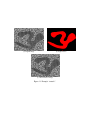
Here it is assumed, that RGB-channels of the image are conditionally independent (modeled by Modalities). Unfortunately it was very difficult for this example to reach good
and reproducible segmentation in fully unsupervised manner. Therefore learning information was included. The “reconstructed” image in fig. 14.c) is produced by subtracting for
each pixel its “shading” part (see description of Gshading).
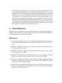
7
Conclusion
First of all we would like no note, that the system objsegm is still in progress. To say
frankly, we do not think, that in the closest time the system will be in such a state, that an
“ordinary user” could use it without going deep in the theory. This is the case, because
only at the moment this theory becomes less or more practicable.
Here is a short list of future work:
– First of all we would like to precise the notation of Parameter. As already said,
they can be seen as a kind of mechanism, which allow to influent statistical models
non locally. At the moment there are still many open questions, both theoretical
and practical ones: how to learn such a kind of parameter, what is common for all
parameter of such kind etc. Therefore in this user manual we only mentioned this
mechanism, but not documented them.
– From the technical side, the system should give the user more possibilities for interactions. In particular interactions during the work should be allowed. Functions for
storing and loading of models should be implemented.
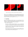
(a) Original image
(b) Segmentation
(c) “Reconstructed” image
Figure 11: Example “tentacle”.
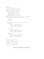
Time:15000
dtime:60
Name:image Type:Map File:tentacle.png code:0
Output:Image {
Name:main {
code:1
code:2
code:3
}
Name:t1
Name:t2
}
Output:Text File:cerr {
Name:main
Name:t1
Name:t2
} Format:Name,n_update,gen_count,timeout
Name:main Type:Split Parent: potts:11. timeout:40
Type:Texture Parent:main Map:image {
Name:t1 height_e:9 width_e:9 s_g:4.
Name:t2 height_e:14 width_e:14 s_g:2.
} step:0.1 n_update:10 min_timeout:0 shad_neigh:500
Figure 12: Description file for the example “tentacle”.
(a) First texture
(b) Second texture
Figure 13: Example “tentacle” – texture images.
(a) Original image
(b) Segmentation
(c) “Reconstructed” image
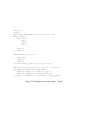
Figure 14: Example “fish”.
Time:6000
Output:Image Name:main code:2
Output:Image Name:main code:3
Output:Text File:cerr Name:main
Type:Map File:fisch_e.ppm {
Name:image_red
code:1
Name:image_green code:2
Name:image_blue code:3
} Format:Name,timeout,gen_count
Name:main Type:Split potts:6 timeout:400 n_update:100
Parent:main Type:Modalities min_timeout:10 {
Name:t1
Name:t2
Name:t3
}
Type:Gshading jump:3 step:0.01 min_timeout:10 {
Parent:t1 {
Name:t1_r Map:image_red
Name:t1_g Map:image_green
Name:t1_b Map:image_blue
}
Parent:t2 {
Name:t2_r Map:image_red
Name:t2_g Map:image_green
Name:t2_b Map:image_blue
}
Parent:t3 {
Name:t3_r Map:image_red
Name:t3_g Map:image_green
Name:t3_b Map:image_blue
}
}
Learn:t1 4 5 846 162
Learn:t2 14 321 100 400
Learn:t2 625 480 686 521
Learn:t3 674 371 771 448
Learn:t3 115 516 414 564
Learn:t3 650 193 840 240
Figure 15: Description file for the example “fish”.
– The main idea of our approach is, that “complex” models can be built using a relatively small number of simple “base” models in an hierarchical manner – i.e. a complex model is a tree-like structure. This reminds of the notation of two-dimensional
grammars (see e.g. [8]). A segmentation model can be understood in this context as
a derivation rule. The main difference from the two-dimensional grammars (in our
opinion) is the fact, that in our method the tree-like structure of a complex model is
fixed. Therefore the hierarchical segmentation approach can be seen as an intermidiate stage between labeling problems and two-dimensional grammars. The question
arises, whether it is possible to extend hierarchical segmentations in such a way, that
the structure of a complex model need not to be fixed.
8
Acknowledgments
This work was done within the scope of an industrial project, funded by Sächsische Aufbaubank. We would like especially to thank our partners from GWT-TUD GmbH, Abt.
Aello for fruitfull discussions and motivations.
References
[1] A. P. Dempster, N. M. Laird, and D. B. Durbin. Maximum likelihood from incomplete data via the EM algorithm. Journal of the Royal Statistical Society, 39:185–197,
1977.
[2] B. Flach. Strukturelle Bilderkennung: Habilitationsschrift. Dresden University of
Technology, 2003. in German.
[3] B. Flach and R. Sara. Joint non-rigid motion estimation and segmentation. In IWCIA04, pages 631–638, 2004.
[4] B. Flach and D. Schlesinger. Best labeling search for a class of higher order gibbs
models. Pattern Recognition and Image Analysis, 14(2):249–254, 2004.
[5] B. Flach, D. Schlesinger, E. Kask, and A. Skulisch. Unifying registration and segmentation for multi-sensor images. In Luc Van Gool, editor, DAGM 2002, LNCS
2449, pages 190–197. Springer, 2002.
[6] Stuart Geman and Donald Geman. Stochastic relaxation, Gibbs distributions, and the
Bayesian restoration of images. IEEE Transactions on Pattern Analysis and Machine
Intelligence, 6(6):721–741, 1984.
[7] I. Kovtun. Texture segmentation of images on the basis of markov random fields.
Technical report, TUD-FI03, May 2003.
[8] Schlesinger M.I. and Hlavác V. Ten Lectures on Statistical and Structural Pattern
Recognition. Kluwer Academic Publishers, Dordrecht, May 2002.
[9] James Gary Propp and David Bruce Wilson. Exact sampling with coupled markov
chains and applications to statistical mechanics. Random Structures Algorithms,
9(1):223–252, 1996.
[10] D. Schlesinger. Gibbs probability distributions for stereo reconstruction. In
B. Michaelis and G. Krell, editors, DAGM 2003, volume 2781 of LNCS, pages 394–
401, 2003.
[11] D. Schlesinger and B. Flach. Transforming an arbitrary minsum problem into a binary one. Technical report, Dresden University of Technology, TUD-FI06-01, April
2005. http://www.bv.inf.tu-dresden.de/∼ds24/tr_kto2.pdf.
[12] Dmitrij Schlesinger. Template based gibbs probability distributions for texture modeling and segmentation. In DAGM-Symposium, pages 31–40, 2006.
[13] M.I. Schlesinger and B. Flach. Some solvable subclasses of structural recognition
problems. In Tomáˆs Svoboda, editor, Czech Pattern Recognition Workshop 2000,
pages 55–62, 2000.
[14] Michail I. Schlesinger. Connection between unsupervised and supervised learning in
pattern recognition. Kibernetika, 2:81–88, 1968. In Russian.