Download MIQL: A Fortran Subroutine for Convex Mixed

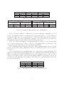
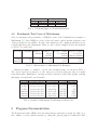
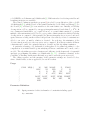
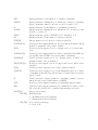
MIQL: A Fortran Subroutine for Convex
Mixed-Integer Quadratic Programming
- User’s Guide T. Lehmann, K. Schittkowski
Address:
Prof. K. Schittkowski
Siedlerstr. 3
D - 95488 Eckersdorf
Germany
Phone:
(+49) 921 32887
E-mail:
[email protected]
Web:
http://www.klaus-schittkowski.de
Date:
October, 2013
Abstract
The Fortran subroutine MIQL solves strictly convex mixed-integer quadratic programming problems subject to linear equality and inequality constraints by a branchand-bound method. The continuous subproblem solutions are obtained by the primaldual method of Goldfarb and Idnani. The code is designed for solving small to medium
size mixed-integer programs. Its usage is outlined and an illustrative example is presented.
Keywords: mixed-integer quadratic programming; quadratic optimization; MIQP; branchand-bound; numerical algorithms
1
1
Introduction
The Fortran subroutine MIQL solves strictly convex-mixed integer quadratic programming
problems subject to linear equality and inequality constraints of the form
T T
x
x
1
T
+d
min 2 x , y C
y
y
x
j = 1, . . . , me ,
aTj
+ bj = 0 ,
y
x ∈ Rn c , y ∈ Nn i :
(1)
x
T
aj
j = me + 1, . . . , m ,
+ bj ≥ 0 ,
y
xl ≤ x ≤ xu ,
yl ≤ y ≤ yu ,
with an n by n positive definite matrix C and n := ni + nc , an n-dimensional vector d,
an m by n matrix A = (a1 , ..., am )T , and an m-vector b. Lower and upper bounds for the
continuous and integer variables, xl , xu , yl and yu respectively, are separately handled. The
objective function of (1) is denoted by
1 T T
x
x
T
f (x, y) = (x , y )C
+d
.
(2)
y
y
2
If ni > 0, the mixed-integer quadratic program (1) is now solved by a branch-and-bound
method.
This manual is organized as follows. The subsequent section introduces the basic concept
of a branch-and-bound method and describes the different options of the underlying Fortran
subroutine. Section 3 describes more details of the implementation, especially the warm
start features. Section 4 summarizes some numerical results to compare different options.
Further implementation details and program documentation are found in Section 5, followed
by an illustrative example in Section 6.
2
The Branch-and-Bound Procedure
A branch-and-bound algorithm starts at the solution of the relaxed problem, in our case the
optimal solution of a continuous quadratic program where the integrality condition y ∈ Nni
is replaced by y ∈ Rni , see also Dakin [3] for an early paper on mixed-integer linear programming. An integer variable yk ∈ I is selected and two different continuous subproblems
are generated. They are obtained by rounding the continuous value of yk , k ∈ I, to get two
separate subproblems, one with upper bound yk , another one with lower bound yk + 1.
2
Each subproblem determines a node in a binary search tree, which is internally created step
by step.
A particular advantage of branch-and-bound methods is that certain subtrees can be
eliminated or fathomed at an early stage before trying all possible combinations by exploring
the whole tree. There are three:
• A subproblem is infeasible: All subsequently generated subproblems obtained by branching from this node would also be infeasible.
• A subproblem has a feasible integer solution. If the corresponding optimal objective
function value is less than a known upper bound, a better upper bound is provided. A
better solution cannot be generated starting from this node.
• Let the optimal value of a non-integral solution of a subproblem be greater than the actual upper bound. Then further branching from the node would only increase function
values, and there is no chance to find a better integer solution.
A branch-and-bound method represents a general framework, which is easily adapted to
other classes of mathematical optimization problems, say linear or nonlinear programming,
see for example Gupta and Ravindran [6]. An essential assumption is the convexity of the
given nonlinear program or the possibility to compute global solutions at all nodes. The
integral node with minimal objective value represents the solution or we get the information
that no feasible mixed-integer solution exists. Note that although the relaxed version of (1)
is assumed to be a strictly convex optimization problem, the solution of the mixed-integer
problem may not be unique. There is also a possibility to exploit lower bounds within a
branch-and-bound algorithm by investigation the dual of (1), see Leyffer and Fletcher [9] for
details.
Thus, there remain decisions by which the numerical performance of a branch-and-bound
algorithm may become influenced:
1. Select an integer variable with a non-integer value in the actual continuous solution of
a node for branching:
(a) maximal fractional branching: Select an integer variable from solution values of a
relaxed subproblem with largest distance from neighbored integer values.
(b) minimal fractional branching: Select an integer variable from solution values of a
relaxed subproblem with smallest distance from neighbored integer values.
2. Search for a free node in the whole tree from where branching, i.e., the generation of
two new subproblems, is initiated:
(a) best of all: All free nodes are compared and a node with lowest objective function
value is selected.
3
(b) best of two: The optimal objective function values of the two child nodes are
compared and the node with a lower value is chosen. If both are leafs, i.e., if the
corresponding solution is integral, or if the corresponding problem is infeasible or
if there is already a better integral solution, strategy best of all is started.
(c) depth first: Select a child node whenever possible. If the node is a leaf, the best
of all strategy is applied.
The depth first strategy has the advantage that the quadratic problem of a child node
can be solved very fast, since the only difference between the both continuous programs is
one additional box constraint. Usually, the search tree is smaller, i.e., there remain less
unexplored nodes. The disadvantage is that the child node is arbitrarily selected leading to
a possibly larger number of subproblems to be solved.
After selecting an integer variable for branching and an unexplored node to continue,
the optimal solutions of the corresponding relaxed quadratic programs are computed. This
process is iterated until all nodes are either explored or fathomed. The upper bound is
infinity until the first integer feasible solution is found.
3
Algorithmic Features of MIQL
An essential component of a branch-and-bound is the ability to solve continuous quadratic
programming problems very efficiently. The primal dual method of Goldfarb and Idnani [5]
is frequently used to solve convex quadratic programs. To exploit as much information as
possible from an existing solution within a branch-and-bound framework, we extend the
Fortran code QL of Schittkowski [13]. This version is called QLX and its calling sequence is
described in the next section.
When called from MIQL, QLX performs warm starts depending on the relationship
between successive subproblems, e.g., in a branch-and-bound procedure:
1. A new node is a child of the actual one, i.e., the new quadratic program is identical to
the previous one apart from one additional box constraint subject to an integer variable.
Since the primal-dual method of Goldfarb and Idnani successively adds constraints to
the active set, we need, in most cases, only one additional iteration to get a new optimal
solution. Even if more iterations are needed, almost always we save some calculation
time compared to a complete new solution of the quadratic program.
2. The new node has the same parent node as the actual one, i.e., both problems differ only
in one box constraint for an integer variable. The algorithm identifies the solution of a
quadratic program by an linearly independent active set. A problem is solved by adding
constraints to and eliminating constraints from the active set, until all constraints are
satisfied, and each iterate is dual feasible. To enable a warm start in the present
situation, one tries first to ensure dual feasibility. This is achieved by saving the active
4
constraints of the common parent node. They are compared to those of the child, i.e.,
the previously solved quadratic program. All other active constraints are eliminated.
Then a dual feasible point is obtained and a new iteration of the algorithm is started
by searching for a violated constraint. Time savings are achieved since in most cases,
only few active constraints have to be deleted and added afterwards.
3. The new node is the child of a node which has the same parent node as the actual
one (nephew): The warm start procedure is similar to the previous one. The only
difference is that active constraints in the two child nodes are compared. This option
is particularly efficient in case of the best of two strategy.
It is possible that warm starts lead to numerical instabilities based on round-off errors.
To avoid this situation, it is possible to limit the number of successive warm starts. In case
of a numerical error, the problem is automatically resolved. Warm starts are indicated by
parameter START of QLX that can obtain the following values:
START
0
10
11
30
31
40
41
42
43
Warm start performed by QLX
Normal execution, no warm starts performed.
Dual warm start, where only bounds are changed.
Dual warm start, where additional constraints are included.
Warm start and early termination, only one QL iteration to be performed.
Warm start and early termination, more than one QL iteration to be performed
as provided by the parameter STEPS.
Remove active constraints from the active set, where the number of these
constraints is stored in the calling parameter NRDC and the indices of the
constraints to be removed are specified in the array DELC.
Remove active constraints from the active set analogue to START = 40, but
continue afterwards with START = 30.
Remove active constraints from the active set analogue to START = 40, but
continue afterwards with START = 31.
Remove active constraints from the active set analogue to START = 40, but
continue afterwards with START = 10.
Table 1: Warm Start Modes
The term dual warm start indicates a situation where a known solution is dual feasible
for the subsequent continuous program. START = 10 is applicable to a child problem during
a branching step.
Furthermore code QLX is able to handle the following special formulation of a quadratic
5
program in an efficiently. Suppose we want to solve a problem of the form
x
x
1
T
T ˆ
T
min
(x , z )C
+d
2
z
z
np
T
T
aj x + a
ˆj z + bj = 0,
j = 1, . . . , me ,
x∈R ,
ˆTj z + bj ≥ 0,
z ∈ Rn−np : aTj x + a
j = me + 1, . . . , m ,
(3)
xl ≤ x ≤ xu ,
zl ≤ z ≤ zu
where Cˆ is an n × n block-diagonal matrix
C
0
,
Cˆ =
0 CD
(4)
where C is a np × np matrix and CD is a (n − np ) × (n − np ) diagonal matrix. np ≤ n can
be considered as reduced problem dimension. a
ˆj is the j-th column of a matrix AD , i.e. the
constraint matrix Aˆ is decomposed in the form
A AD ,
(5)
Aˆ =
where A is a m × np matrix and AD is an m × (n − np ) diagonal matrix. This problem
formulation (3) arises, e.g., when a quadratic program is relaxed by the introduction of m
additional slack variables to ensure feasibility, or in special data mining problems related to
support vector machines, see Schittkowski [14].
There are further features of our new version of our branch-and-bound code MIQL:
1. The new depth first search benefits from warm starts.
2. Since a node marked by a fathoming rule, is not needed any longer, the node data will
become overwritten.
3. In case of false termination when solving a quadratic program, the whole process is
not terminated and the error is treated in the same way as an infeasible leaf.
4. Improved bounds according to Leyffer and Fletcher [9] are calculated, if nodes are
selected by best of all, by using warm start options START = 30 and START = 41 of
QLX.
5. The branching direction for depth first search is determined by evaluating the Layj , where j is the selected branching variable and
grangian function at ˆ
yj and ˆ
(ˆ
x, yˆ) the solution of the previous branch-and-bound QP.
6
6. Lagrangian multipliers are be calculated independently of the solution method by a
modified least squares approach, which uses an extended QP formulation to guarantee
feasibility. This calculation is executed, if storage for (2n + m + 4)2 branch-and-bound
nodes is provided. Otherwise, multipliers would depend, e.g., on the node selection
strategy and the branching rule. Independent multipliers are especially useful, if MIQL
is used as subproblem solver for the mixed-integer nonlinear solver MISQP of Exler
and Schittkowski [4], since then Lagrangian multipliers are needed to calculate a BFGS
update.
4
4.1
Numerical Results
MISQP Subproblems
All numerical results are obtained on a Intel E6600 Dual Core CPU with 2.4 GHz under
Windows XP 64 using Intel Fortran Compiler version 9.1.
For testing the nonlinear mixed-integer code MISQP, a large number of test problems
have been implemented by Exler and Schittkowski [4]. Since in each iteration of the SQPbased method, a mixed-integer quadratic programming problem must be solved by MIQL,
a large number of test examples is available. A subset of 35 MIQP subproblems is selected
with calculation times over 0.1 seconds. Table 2 shows some characteristic data of the
corresponding nonlinear programs.
problem
MITP57
MITP60
MITP62
MITP63
MITP66
MITP83
MITP115
MITP116
MITP117
continuous
variables
2
0
0
0
16
0
9
9
9
integer
variables
4
24
35
48
19
20
27
27
27
inequality
constraints
0
35
44
53
1
20
12
12
12
equality
constraints
1
0
0
0
17
0
9
9
9
Table 2: Problem Characteristics
Most of those test examples are selected from the GAMS MINLP-Library, see Bussieck,
Drud, and Meeraus [2]. Some are simple case studies from petroleum industry. Problems
MITP115, MItp116, and MItp117 have multiple global optima. In the subsequent tables,
the total number of branch-and-bound nodes and the total calculation times are reported.
For comparing all other options, we always choose the fastest alternative.
7
best of all
nodes time (sec)
115,588
36.3
best of two
nodes time (sec)
121,996
26.5
depth first
nodes time (sec)
122,055
26.4
Table 3: Node Selection Strategy
best of two
warm start
no warm start
nodes time (sec) nodes time (sec)
121,996
26.5
122,516
33.8
depth first
warm start
no warm start
nodes time (sec) nodes time (sec)
122,055
26.4
121,739
33.6
Table 4: Performance Improvements due to Warm Starts
Table 3 shows the influence of different node selection strategies. Although best of all
leads to the smallest amount of continuous QP problems that have to be solved during the
branch-and-bound process, calculation time is considerably higher than for the other two
strategies because of very few warm starts. Strategies best of two and depth first guided by
the Lagrangian function value exhibit nearly identical performance.
Next, we consider the influence of warm starts subject to the node selection strategies
best of two and depth first, see Table 4. For best of all warm starts can be neglected. We
observe that warm starts improve the performance significantly.
The branching direction is chosen by the value of the Lagrangian function in case of depth
first to prevent blind diving. Significant reduction of branch-and-bound nodes is achieved,
see Table 5.
Table 6 shows the effect of calculating improved bounds leading to faster fathoming. The
improved bounds exploit dual information and are calculated by an additional QL iteration.
Improved bounds, see Leyffer and Fletcher [9], are only calculated in case of the best of all
strategy. The results of Table 6 show that although the number of branch-and-bound nodes
is reduced by early fathoming, the calculation of the improved bound information slows down
the overall performance.
Lagrangian
nodes time (sec)
122,055
26.4
no Lagrangian
nodes time (sec)
302,145
44.5
Table 5: Branching Direction by Lagrangian Function
8
improved bounds
nodes time (sec)
115,588
36.3
no improved bounds
nodes
time (sec)
99,717
40.3
Table 6: Calculating Improved Bounds Information
4.2
Benchmark Test Cases of Mittelmann
Next, we investigate the performance of MIQL for some of the benchmark test examples of
Mittelmann [10]. Since MIQL is a dense solver and cannot exploit sparsity patterns, some
of the problems are not suitable. In some other situations, the continuous relaxation is not
solvable without special adjustments. Thus, we only consider examples ibell3a and imas284,
see Table 7 for some data.
problem
constraints
ibell3a
imas284
104
68
number of
variables
number of non-zero density non-zero density
integer
of constraint
of objective
variables
matrix function matrix
122
60
3.1%
0.4%
151
150
95.3%
0.6%
Table 7: Characteristics of Mittelmann Test Examples
Numerical results, i.e., number of nodes and calculation time, are shown in Table 8.
The option depth first is superior to the other node selection strategies, since it benefits
from warm starts. Furthermore, an integer feasible solution is often found quickly, enabling
fathoming of branch-and-bound branches.
problem
ibell3a
ibell3a
ibell3a
imas284
imas284
imas284
branching strategy
maximal fraction
maximal fraction
maximal fraction
maximal fraction
maximal fraction
maximal fraction
node selection
best of all
best of two
depth first
best of all
best of two
depth first
nodes time (sec)
61,588
1,201
63,777
1,125
74,720
952
142,241
3,610
186,412
3,576
142,434
1,940
Table 8: Results for Mittelmann Test Examples without Cuts
5
Program Documentation
The Fortran subroutine MIQL solves the mixed-integer quadratic program (1) with a positive definite objective function matrix by calling the general purpose branch-and-bound
9
code BFOUR, see Lehmann and Schittkowski [8]. Different rules for selecting variables and
branching strategies are available.
The relaxed continuous quadratic program (1) is solved by a modification of the code QL
of Schittkowski [13], which is based on the primal-dual method of Goldfarb and Idnani [5], see
also Powell [11] or Boland [1] for an extension to the semi-definite case. Initially, a Cholesky
decomposition of C is computed by an upper triangular matrix R such that C = RT R. In
case of numerical instabilities, e.g., round-off errors, or a semi-definite matrix C, a certain
multiple of the unit matrix is added to C to get a positive definite matrix for which a Cholesky
decomposition is computed. Subsequently, the known triangular factor is saved and used
again, whenever solving another relaxed subproblem. Successively, violated constraints are
added to an active set until a solution is obtained. In each step, the minimizer of the
objective function subject to the new active set is computed. If an iterate satisfies all linear
constraints and bounds, the optimal solution is obtained and the algorithm terminates.
A particular advantage of a dual method is that phase I of a primal algorithm, i.e., the
computation of an initial feasible point satisfying all linear constraints and bounds, can be
avoided. The algorithm proves its robustness and efficiency in the framework of sequential
quadratic programming algorithm, see Schittkowski [12, 15]. A further advantage is the
possibility of handling warm starts efficiently as pointed out in the previous section.
The calling sequence and the meaning of the parameter settings are described below,
where default values, as far as applicable, are set in brackets.
Usage:
CALL
MIQL (
/
/
/
/
/
/
M,
ME, MMAX,
N, NMAX,
MNN,
NI,
IND,
C,
D,
A,
B,
XL,
XU,
X,
U,
F,
ACC,
EPS,
IOPT,
ROPT, LOPT,
IOUT, IFAIL, IPRINT,
RW,
LRW,
IW,
LIW,
LW,
LLW
)
Parameter Definition:
M:
Input parameter for the total number of constraints including equality constraints.
10
ME :
MMAX :
N:
NMAX :
MNN :
NI :
IND(NI) :
C(NMAX,N) :
D(N) :
A(MMAX,N) :
B(MMAX) :
XL(N),XU(N) :
X(N) :
U(MNN) :
F:
ACC :
EPS :
IOPT(20) :
IOPT(1)
IOPT(2)
Input parameter for the number of equality constraints.
Input parameter defining the row dimension of array A containing
linear constraints, must be at least one and or equal to M.
Input parameter for the number of optimization variables.
Input parameter defining the row dimension of C, at least one and
greater or equal to N.
Input parameter equal to MMAX+N+N, dimension of U.
Input parameter for the number of integer variables.
Integer input vector for indices of integer variables.
Double precision input matrix for objective function matrix, which
should be symmetric and positive definite.
Double precision input vector for constant vector of objective function.
Double precision input matrix for linear constraints, first ME rows
for equality, then M-ME rows for inequality constraints.
Double precision input vector for constant values of linear constraints in same order as matrix A.
Double precision input vectors for upper and lower bounds of the
variables.
Double precision output vector for the optimal solution.
Double precision output vector for the multipliers subject to linear
constraints at the first M positions and for bounds, first lower then
upper bounds.
Double precision output parameter containing optimal objective
function value at successful return, see IFAIL.
Double precision input parameter for identifying integer values.
Double precision input parameter for termination accuracy of the
QP solver QL, should not be smaller than machine precision.
Integer option array:
Branching rule,
1 : Maximal fractional branching.
2 : Minimal fractional branching.
Node selection strategy,
1 : Best of all.
11
IOPT(3)
IOPT(4)
IOPT(5)
IOPT(6)
IOPT(7)
IOPT(12)
IOPT(14)
ROPT(20) :
LOPT(20) :
IOUT :
IFAIL :
2 : Best of two.
3 : Depth first.
Maximal number of nodes (100,000).
Maximal number of successive warmstarts to avoid numerical instabilities (100).
Calculate improved bounds if best-of-all node selection strategy is
used (0).
Select direction for depth-first according to value of Lagrange function (0).
Cholesky decomposition mode (1),
0 : Calculate Cholesky decomposition once and reuse it.
1 : Calculate new Cholesky decomposition whenever warmstart is
not activate.
Input parameter for the reduced quadratic program dimension (N).
Output parameter for total number of branch-and-bound nodes.
Double precision option array to remain compatible with previous
versions.
Logical option array to remain compatible with previous versions.
Input parameter for desired output unit number, i.e., all writestatements start with ’WRITE(IOUT,... ’.
Output parameter for termination reason:
-4 : Branch-and-bound root QP not solvable.
-3 : Relaxed QP without feasible solution.
-2 : Feasible solution could not be computed within maximal number of nodes.
-1 : Feasible integer solution does not exist.
0 : Optimal solution found.
1 : Feasible solution found, but the maximum number of nodes
reached.
2 : Index in IND out of bounds.
3 : Termination due to internal inconsistency of branch-and-bound
routine BFOUR.
4 : Length of a working array RW, IW, or LW too small.
12
IPRINT :
RW(LRW) :
LRW :
IW(LIW) :
LIW :
5 : Parameters N, M, MNN, ME, or NI incorrect.
6 : Option of IOPT incorrectly set.
7 : Independent Lagrangian multipliers could not be calculated,
primal solution is valid. Increase IOPT(3) for performing independent Lagrangian multiplier calculation.
8 : IOUT or IPRINT incorrectly set.
9 : Lower variable bound greater than upper one.
10 + i : Problem is continuous and could not be solved due to error
i of QP solver QL, see corresponding documentation.
100 + i : Problem is continuous and infeasible, constraint i could
not be included in active set.
Input parameter defining the output level:
0 : No output to be generated.
1 : Root QP and final performance summary.
2 : Additional branch and bound iterations counter.
3 : Additional output from all generated subproblems:
* : fractional feasible node,
B : new best integer feasible solution,
I
: infeasible node,
M : marked node,
3 : Complete output for all nodes, e.g., with bounds.
4 : Full debug output.
Double precision working array of length LRW
Input parameter for length of RW, must be at least
5*NMAX*NMAX/2 + 7*NI + 10*NMAX + 3*MMAX + 8*N +
3*MAXNDS + 33
Integer working array of length LIW
Input parameter for length of IW, must be at least NMAX + NI +
MMAX + 6*MAXNDS + 4*N + 30
13
LW(LLW) :
LLW :
6
Logical working array of length LLW
Input parameter for length of LW, must be at least 3*NI + 23
Example
To give an example, we consider the simple quadratic program
min 12 5i=1 x2i − 21.98x1 − 1.26x2 + 61.39x3 + 5.3x4 + 101.3x5
x1 , x2 ∈ R,
−7.56x1 + 0.5x5 + 39.1 ≥ 0 ,
x3 , x4 , x5 ∈ N :
−100 ≤ xi ≤ 100 , i = 1 . . . , 5
The corresponding Fortran source code is listed below.
IMPLICIT
INTEGER
PARAMETER
NONE
NMAX, MMAX, MNNMAX, LIW, LRW, LLW, MAXNDS
(NMAX
= 5,
/
MMAX
= 1,
/
MAXNDS = 1000,
/
MNNMAX = MMAX + NMAX + NMAX,
/
LIW
= 6*NMAX + MMAX + 6*MAXNDS + 30,
/
LRW
= 5*NMAX*NMAX/2 + 25*NMAX + 3*MMAX
/
+ 3*MAXNDS + 33,
/
LLW
= 3*NMAX + 23)
INTEGER
M, ME, N, MNN, NI, IND(NMAX), IOUT, IFAIL,
/
IPRINT, IW(LIW), I, J, IOPT(20)
DOUBLE PRECISION F, ACC, EPS, A(MMAX,NMAX), C(NMAX,NMAX), B(MMAX),
/
D(NMAX), XL(NMAX), XU(NMAX), X(NMAX), U(MNNMAX),
/
RW(LRW), ROPT(20)
LOGICAL
LW(LLW), LOPT(20)
C
C
C
Set parameters
N
= 5
M
= 1
ME
= 0
MNN
= MMAX + N + N
NI
= N
ACC
= 1.0D-10
EPS
= 1.0D-12
IPRINT = 2
IOUT
= 6
DO I=1,20
ROPT(I) = -1.0D0
IOPT(I) = -1
LOPT(I) = .TRUE.
END DO
IOPT(1) = 1
IOPT(2) = 1
IOPT(3) = MAXNDS
C
C
C
Set problem data
DO I=1,N
DO J=1,N
C(I,J) = 0.0D0
14
END DO
C(I,I) =
1.0D0
A(1,I) =
0.0D0
XL(I) = -100.0D0
XU(I) = 100.0D0
END DO
DO I=1,NI
IND(I) = I
END DO
A(1,1) = -7.56D0
A(1,5) =
0.5D0
B(1)
=
39.1D0
D(1)
= -21.98D0
D(2)
= -1.26D0
D(3)
= 61.39D0
D(4)
=
5.3D0
D(5)
= 101.3D0
C
C
C
Call MIQL
CALL MIQL(
/
/
/
/
/
/
M,
MNN,
A,
U,
ROPT,
RW,
LLW )
ME,
NI,
B,
F,
LOPT,
LRW,
MMAX,
IND,
XL,
ACC,
IOUT,
IW,
N,
NMAX,
C,
D,
XU,
X,
EPS,
IOPT,
IFAIL, IPRINT,
LIW,
LW,
C
STOP
END
The following output should appear on screen:
MIQL - A branch and bound mixed integer quadratic solver
***
***
***
***
***
***
INFO
INFO
INFO
INFO
INFO
INFO
(MIQL):
(MIQL):
(MIQL):
(MIQL):
(MIQL):
(MIQL):
Maximal number of successive warmstarts set to zero!
Improved bound computation deactivated!
Lagrangian direction deactivated!
Cholesky decomposition mode set to 1!
Reduced QP dimension set to original dimension!
Initial number of branch and bound nodes set to zero!
Parameters:
Maximal branch and bound nodes
Node selection strategy
Branching variable selection
Improved bounds calculation
Lagrangian direction
QL decomposition mode
Maximal successive warmstarts
=
=
=
=
=
=
=
1000
1
1
0
0
1
0
-------------------------------------------------------------------Start of the Mixed-Integer Branch and Bound Code BFOUR
Version 3.0 (Mar 2013)
--------------------------------------------------------------------
15
Parameters:
Number of integer variables
5
Maximal number of nodes
1000
Integer tolerance
0.10D-09
Branching strategy
1
Node selection
1
Convex problem
No initial integer feasible solution known
Output in the following order:
S
- status of current node
B ... branched node
I ... infeasible node
M ... marked node
* ... other node
IT
- iteration count
ND
- index of current node
F
- objective function value
P
- index of parent node
LB
- lower bound
UB
- upper bound
S
IT
ND
F
P
LB
UB
-----------------------------------------------------------------------*
1
1 -.699651D+04
0 -.699651D+04 0.100000D+31
*
2
2 -.698324D+04
1 -.699651D+04 0.100000D+31
*
3
3 -.697573D+04
1 -.699651D+04 0.100000D+31
*
4
4 -.698317D+04
2 -.698324D+04 0.100000D+31
*
5
5 -.698306D+04
2 -.698324D+04 0.100000D+31
*
6
6 -.698312D+04
4 -.698317D+04 0.100000D+31
*
7
7 -.698292D+04
4 -.698317D+04 0.100000D+31
B
8
8 -.698285D+04
6 -.698312D+04 -.698285D+04
B
9
8 -.698309D+04
6 -.698312D+04 -.698309D+04
Optimal solution:
Number of explored subproblems:
Highest index:
7
F(Y)
=
-6983.0900
Y(
1) =
-2.0000000
Y(
2) =
1.0000000
Y(
3) =
-61.000000
Y(
4) =
-5.0000000
Y(
5) =
-100.00000
9
*** INFO (MIQL): QPs with numerical problems =
0
Optimal solution of original problem:
Objective
X(
1)
X(
2)
X(
3)
X(
4)
X(
5)
function value:-6983.090000
=
-2.0000000
=
1.0000000
=
-61.000000
=
-5.0000000
=
-100.00000
Some further quadratic programs for testing a correct implementation are found in Hock
and Schittkowski [7].
16
References
[1] Boland N.L. (1997): A dual-active-set algorithm for positive semi-definite quadratic
programming, Mathematical Programming, Vol. 78, 1-27
[2] Bussieck M.R., Drud A.S., Meeraus A. (2007): MINLPLib - A collection of test models for mixed-integer nonlinear programming, GAMS Development Corp., Washington
D.C., USA
[3] Dakin R.J. (1965): A tree search algorithm for mixed-integer programming problems,
Computer Journal, Vol. 8, 250-255
[4] Exler O., Schittkowski K. (2006): MISQP: A Fortran implementation of a trust region
SQP algorithm for mixed-integer nonlinear programming - User’s guide, version 2.0,
Report, Department of Computer Science, University of Bayreuth, Germany
[5] Goldfarb D., Idnani A. (1983): A numerically stable method for solving strictly convex
quadratic programs, Mathematical Programming, Vol. 27, 1-33
[6] Gupta O.K., Ravindran A. (1985): Branch-and-bound experiments in convex nonlinear
integer programming, Management Science, Vol. 31, 1533-1546
[7] Hock W., Schittkowski K. (1981): Test Examples for Nonlinear Programming Codes,
Lecture Notes in Economics and Mathematical Systems, Vol. 187, Springer
[8] Lehmann T., Schittkowski K. (2008): BFOUR: A Fortran subroutine for integer optimization by branch-and-bound - user’s guide -, Report, Department of Computer
Science, University of Bayreuth, Germany
[9] Leyffer S., Fletcher R. (1998): Numerical experiments with lower bounds for MIQP
branch-and-bound, SIAM Journal on Optimization, Vol. 8, 604-616
[10] Mittelmann H. (2007): Mixed-integer (QC) QP benchmark,
http://plato.asu.edu/ftp/miqp.html
[11] Powell M.J.D. (1983): ZQPCVX, A Fortran subroutine for convex quadratic programming, Report DAMTP/1983/NA17, University of Cambridge, England
[12] Schittkowski K. (1985/86): NLPQL: A Fortran subroutine solving constrained nonlinear programming problems, Annals of Operations Research, Vol. 5, 485-500
[13] Schittkowski K. (2003): QL : A Fortran code for convex quadratic programming User’s guide, Report, Department of Mathematics, University of Bayreuth, Germany
[14] Schittkowski K. (2005): Optimal parameter selection in support vector machines, Journal of Industrial and Management Optimization, Vol. 1, 465-476
17
[15] Schittkowski K. (2006): NLPQLP: A Fortran implementation of a sequential quadratic
programming algorithm with distributed and non-monotone line search - user’s guide,
version 2.2, Report, Department of Computer Science, University of Bayreuth, Germany
18