1
TSSpredator User Guide
v 1.00
Alexander Herbig
[email protected]
Kay Nieselt
[email protected]
June 3, 2013
1
Getting Started
TSSpredator is a tool for the comparative detection of transcription start
sites (TSS) from RNA-seq data. It can integrate data from different experimental conditions but also from different organisms on the basis of a multiple
whole-genome alignment.
There are two ways to use TSSpredator. The most convenient way is
to use its graphical user interface (GUI), which is described in section 3.
Here, all settings and parameters can be specified that are needed for the
prediction. For a detailed description of the parameters see section 4. After
setting up the study the configuration can be saved. Pressing the RUN button
starts the prediction procedure. All results are saved in the specified output
folder. The most important result file is the Master Table (MasterTable.tsv ).
For a detailed description of all result files see section 5.
Another way to utilize TSSpredator is via its command line interface. This is especially useful for automatization or integration in an analysis
pipeline. For this, TSSpredator has to be started with a single argument,
which is the path of a configuration file, as it is saved by TSSpredator’s
GUI. For example:
java -Xmx1G -jar TSSpredator.jar config.conf
1
2
2.1
Methods
Normalization
Before the comparative analysis we normalize the expression graph data that
is used as input. A percentile normalization step is applied to normalize the
graphs from the enriched library. For this the 90th percentile (default, see
normalization percentile) of all data values is calculated for each graph of a
treated library. This value is then used to normalize this graph as well as
the respective graph of the untreated library. Thus, the relative differences
between each pair of libraries (treated and untreated) are not changed in this
normalization step. All graphs are multiplied with the overall lowest value
to restore the original data range.
To account for different enrichment rates a further normalization step is
applied. During this step a prediction of TSS candidates is performed for each
strain/condition. These candidates are then used to determine the median
enrichment factor for each library pair (default, see enrichment normalization
percentile). Using these medians all untreated libraries are then normalized
against the library with the strongest enrichment.
2.2
The SuperGenome
To be able to assign TSS that have been detected in different genomes to
each other TSSpredator computes a common coordinate system for the
genomes. This is done on the basis of a whole-genome alignment. For the
generation of whole-genome alignments the software Mauve can be used, for
example. It is able to detect genomic rearrangements and builds multiple
whole-genome alignments as a set of collinearly aligned blocks. The resulting xmfa file is then read by TSSpredator and the alignment information
in the blocks is used to calculate a joint coordinate system for the aligned
genomes and mappings between this coordinate system and the original genomic coordinates. In addition to the cross-genome comparison of detected
TSS this allows for an alignment of RNA-seq expression graphs, which can
then be visualized in a genome browser. If different experimental conditions
are compared with the same genome, the SuperGenome construction step is
skipped (see Type of Study setting).
2.3
TSS Prediction
The initial detection of TSS in the single strains/conditions is based on the
localization of positions, where a significant number of reads start. Thus, for
2
each position i in the RNA-seq graph corresponding to the treated library the
algorithm calculates e(i)−e(i−1), where e(i) is the expression height at position i. In addition, the factor of height change is calculated, i.e. e(i)/e(i − 1).
To evaluate if the reads starting at this position are originating from primary transcripts the enrichment factor is calculated as etreated (i)/euntreated (i).
For all positions where these values exceed the threshold a TSS candidate
is annotated. If the TSS candidate reaches the thresholds in at least one
strain/condition the thresholds are decreased for the other strains/conditions.
We declare a TSS candidate to be enriched in a strain/condition if the respective enrichment factor reaches the respective threshold. A TSS candidate has
to be enriched in at least one strain/condition and is discarded otherwise. If
a TSS candidate does not appear to be enriched in a strain/condition but
still reaches the other thresholds it is only indicated as detected. However,
a TSS candidate can only be labeled as detected in a condition if its untreated expression value does not exceed its treated expression value by a
factor higher than the chosen processing site factor. Otherwise we consider
it to be a processing site. TSS candidates that are in close vicinity (TSS
cluster distance) are grouped into a cluster and by default only the TSS candidate with the highest expression is kept (see cluster method ). The final
TSS annotations are then characterized with respect to their occurrence in
the different strains/conditions and in which strain/condition they appear to
be enriched. The TSS are then further classified according to their location
relative to annotated genes. For this we used a similar classification scheme
as previously described (Sharma et al., 2010). Thus for each TSS it is decided
if it is the primary or secondary TSS of a gene, if it is an internal TSS, an
antisense TSS or if it cannot be assigned to one of these classes (orphan). A
TSS is classified as primary or secondary if it is located upstream of a gene
not further apart than the chosen UTR length. The TSS with the strongest
expression considering all conditions is classified as primary. All other TSS
that are assigned to the same gene are classified as secondary. Internal TSS
are located within an annotated gene on the sense strand and antisense TSS
are located inside a gene or within a chosen maximal distance (antisense
UTR length) on the antisense strand. These assignments are indicated by
a 1 in the respective column of the Master Table. Orphan TSS, which are
not in the vicinity of an annotated gene, are indicated by zeros in all four
columns.
3
Figure 1: Screenshot of the TSSpredator graphical user interface.
A: General settings for the study. B: TSS prediction parameters and other settings.
C: Genome/Condition specific settings and files. D: Message area, where information
about the prediction procedure is displayed. E: Buttons to Load or Save a configuration.
F: RUN button to start the prediction procedure. The Cancel button stops a running
prediction.
3
The User Interface
Study setup In the study setup area (Figure 1A) general settings for the
study can be made. Most importantly these are the type of the study (comparison of strains (requires alignment file) or conditions), the number of
genomes/conditions and replicates, and the path to the output directory. A
project name can also be specified.
Parameter area In the parameter area (Figure 1B) specific parameters of
the TSS prediction procedure can be changed. Instead of changing individual
parameters it is also possible to select a parameter preset from the drop-down
menu.
4
Genome/Condition related settings For each genome/condition of the
study a tab is generated (Figure 1C), in which settings specific for this
genome/condition can be made. This includes the name and ID, and
file paths to the genomic sequence (FASTA) and the genome annotation
(GFF). In addition, for each replicate a tab is displayed within the respective genome/condition tab, where the RNA-seq wiggle files of the replicate
can be entered.
Message Area In the message area (Figure 1D) information about a running prediction process is displayed. Thus, it can be easily determined in
which step a running prediction procedure currently is. At the end of the
procedure a brief summary is shown.
Load/Save Configuration Using the Save or Load button (Figure 1E)
a configuration including all settings can be saved, or a previously saved
configuration can be loaded, respectively. Loading a configuration overwrites
all current settings.
Run prediction By pressing the RUN button (Figure 1F) the prediction
procedure is started using the current settings and parameters. Information
about the running process is displayed in the message area. The running
prediction can be canceled using the Cancel button. Note that this might
result in incomplete output files.
4
4.1
Settings and Parameters
Study Setup
Project Name Enter a name for the study.
Type of Study Chose between Comparison of different conditions and
Comparison of different strains/species.
For a cross-strain analysis an Alignment file has to be provided (see below).
In addition, in each genome tab an individual genomic sequence and genome
annotation has to be set.
When comparing different conditions no alignment file is needed and the
genomic sequence and genome annotation of the organism has to be set in
the first genome tab only.
5
Number of Genomes Set the number of different strains/conditions
in the study. Press the ’Set’ button to generate a settings tab for each
strain/condition and each replicate of the study.
Number of Replicates Set the number of different replicates for each
strain/condition. Press the ’Set’ button to generate a settings tab for each
strain/condition and each replicate of the study.
Output Data Path Select the folder in which all result files will be placed.
Alignment File Select the xmfa alignment file containing the aligned
genomes. If the study compares different conditions, this field is inactive.
4.2
TSS prediction parameters
In the following the parameters affecting the TSS prediction procedure are
described. Instead of changing the parameters manually it is also possible
to select predefined parameters sets using the parameter presets drop-down
menu.
step height This value relates to the minimal number of read starts at a
certain genomic position to be considered as a TSS candidate. To account
for different sequencing depths this is a relative value based on the 90th
percentile of the expression height distribution. A lower value results in a
higher sensitivity.
step height reduction When comparing different strains/conditions and
the step height threshold is reached in at least one strain/condition, the
threshold is reduced for the other strains/conditions by the value set here.
A higher value results in a higher sensitivity. Note that this value must be
smaller than the step height threshold.
step factor This is the minimal factor by which the TSS height has to
exceed the local expression background. This feature makes sure that a TSS
candidate has to show a higher expression in regions of locally high expression than would be necessary in regions where no expression background is
detected. A lower value results in a higher sensitivity. Set this value to 1 to
disable the consideration of the local expression level.
6
step factor reduction When comparing different strains/conditions and
the step factor threshold is reached in at least one strain/condition, the
threshold is reduced for the other strains/conditions by the value set here.
A higher value results in a higher sensitivity. Note that this value must be
smaller than the step factor threshold.
enrichment factor The minimal enrichment factor for a TSS candidate.
The threshold has to be exceeded in at least one strain/condition. If the
threshold is not exceeded in another condition the TSS candidate is still
marked as detected but not as enriched in this strain/condition. A lower value
results in a higher sensitivity. Set this value to 0 to disable the consideration
of the enrichment factor.
processing site factor The maximal factor by which the untreated library
may be higher than the treated library and above which the TSS candidate
is considered as a processing site and not annotated as detected. A higher
value results in a higher sensitivity.
step length Minimal length of the TSS related expression region (in base
pairs). This value depends on the length of the reads that are stacking at the
TSS position. In most cases this feature can be disabled by setting it to ’0’.
However, it can be useful if RNA-seq reads have been trimmed extensively
before mapping.
base height This value relates to the minimal number of reads in the nonenriched library that start at the TSS position. This feature is disabled by
default.
4.3
Normalization Settings
normalization percentile By default a percentile normalization is performed on the RNA-seq data. This value defines the percentile that is used
as a normalization factor. Set this value to ’0’ to disable normalization.
enrichment normalization percentile By default a percentile normalization is performed on the enrichment values. This value defines the percentile that is used as a normalization factor. Set this value to ’0’ to disable
normalization.
7
4.4
Output options
write RNA-seq graphs If this option is enabled, the normalized RNAseq graphs are written into the output folder. Disable this option, if the
normalized graphs are not needed or if they have been written before. Note
that writing the graphs will increase the runtime.
4.5
TSS Clustering Settings
cluster method TSS candidates in close vicinity are clustered and only
one of the candidates is kept. HIGHEST keeps the candidate with the highest
expression. FIRST keeps the candidate that is located most upstream.
TSS clustering distance This value determines the maximal distance (in
base pairs) between TSS candidates to be clustered together. Set this value
to ’0’ to disable clustering.
4.6
Comparative Settings
allowed cross-genome/condition shift This is the maximal positional
difference (bp) for TSS candidates from different strains/conditions to be
assigned to each other.
allowed cross-replicate shift This is the maximal positional difference
(bp) for TSS candidates from different replicates to be assigned to each other.
matching replicates This is the minimal number of replicates in which a
TSS candidate has to be detected. A lower value results in a higher sensitivity.
4.7
Classification Settings
UTR length The maximal upstream distance (in base pairs) of a TSS
candidate from the start codon of a gene that is allowed to be assigned as a
primary or secondary TSS for that gene.
antisense UTR length The maximal upstream or downstream distance
(in base pairs) of a TSS candidate from the start or end of a gene to which
the TSS candidate is in antisense orientation that is allowed to be assigned
as an antisense TSS for that gene. If the TSS is located inside the coding
region on the antisense strand it is also annotated as an antisense TSS.
8
4.8
Genome specific Settings
Name Brief unique name for this strain/condition, which can be freely
chosen. As this name is also used in some filenames any special characters
(including spaces) should be avoided.
Alignment ID The identifier of this genome in the alignment file. If
Mauve was used to align the genomes, the identifiers are just numbers
assigned to the genomes in the order as they have been chosen as input in
Mauve.
The first lines of the alignment file should also contain this information:
#FormatVersion Mauve1
#Sequence1File genomeA.fa
#Sequence1Format FastA
#Sequence2File genomeB.fa
#Sequence2Format FastA
In this example ‘genomeA’ has ID 1 and ‘genomeB’ has ID 2.
When loading an alignment file (xmfa) TSSpredator tries to set the
alignment IDs automatically.
genome FASTA FASTA file containing the genomic sequence of this
genome.
genome annotation GFF file containing genomic annotations for this
genome (as can be downloaded from NCBI).
4.9
Graph Files
enriched plus Select the file containing the RNA-seq expression graph for
the plus strand (forward) from the 5’ enrichment library.
enriched minus Select the file containing the RNA-seq expression graph
for the plus strand (forward) from the library without 5’ enrichment.
normal plus Select the file containing the RNA-seq expression graph for
the minus strand (reverse) from the 5’ enrichment library.
normal minus Select the file containing the RNA-seq expression graph for
the minus strand (reverse) from the library without 5’ enrichment.
9
5
5.1
Output
Master Table (MasterTable.tsv)
This table contains information on positions and class assignments of all
automatically annotated TSS. The table consists of the following columns:
SuperPos The position of the TSS in the SuperGenome.
SuperStrand The strand of the TSS in the SuperGenome.
MapCount Number of strains into which the TSS can be mapped. Separate entry lines exist for each strain to which the TSS can be mapped whether
the TSS was detected in that strain or not.
detCount The number of strains/conditions in which this TSS was detected in the RNA-seq data.
Condition The identifier of the strain/condition to which the rest of the
line relates.
detected Contains a ’1’ if the TSS was detected in this strain/condition.
enriched Contains a ’1’ if the TSS is enriched in this strain/condition.
stepHeight The expression height change at the position of the TSS. This
relates to the number of reads starting at this position. (e(i) - e(i-1); e(i):
expression height at position i)
stepFactor The factor of height change at the position of the TSS.
(e(i)/e(i-1); e(i): expression height at position i)
enrichmentFactor The enrichment factor at the position of the TSS.
classCount The number of classes to which this TSS was assigned.
Pos Position of the TSS in that genome.
Strand Strand of the TSS in that genome.
10
Locus tag The locus tag of the gene to which the classification relates.
Product The product description of this gene.
UTRlength The length of the untranslated region between the TSS and
the respective gene (nt). (Only applies to ’primary’ and ’secondary’ TSS.)
GeneLength The length of the gene (nt).
Primary Contains a ’1’ if the TSS was classified as ’primary’ with respect
to the gene stated in ’locusTag’.
Secondary Contains a ’1’ if the TSS was classified as ’secondary’ with
respect to the gene stated in ’locusTag’.
Internal Contains a ’1’ if the TSS was classified as ’internal’ with respect
to the gene stated in ’locusTag’.
Antisense Contains a ’1’ if the TSS was classified as ’antisense’ with respect to the gene stated in ’locusTag’.
Automated Contains a ’1’ if the TSS was detected automatically.
Manual Contains a ’1’ if the TSS was annotated manually.
Putative sRNA Contains a ’1’ if the TSS might be related to a novel
sRNA. (Not evaluated automatically)
Putative asRNA Contains a ’1’ if the TSS might be related to an asRNA.
Sequence -50 nt upstream + TSS (51nt) Contains the base of the TSS
and the 50 nucleotides upstream of the TSS.
5.2
Supplemental Files
strain super.fa Contains the genome sequence of each strain mapped to
the coordinate system of the SuperGenome. All 4 files together actually
contain the whole-genome alignment. These files can be used in genome
browsers that allow the user to load several sequences simultaneously.
11
strain super.gff Contains the gene annotations of each strain mapped to
the coordinate system of the SuperGenome.
strain superTypeStrand.gr Contains the xy-graphs of each strain
mapped to the coordinate system of the SuperGenome. Type is either
’FivePrime’ (treated) or ’Normal’ (untreated). Strand is either ’Plus’ or
’Minus’. Note that the files now contain the value 0.0001 instead of 0 as a
value of 0 (i.e. no entry line) now indicates a gap. This is necessary for IGB’s
thresholding feature (see below).
superTSS.gff Contains all TSS predicted in the four strains in the coordinate system of the SuperGenome. Also all TSS that were only predicted
in one strain are listed. The information in how many strains (and in which)
a TSS was detected is given in superClasses.tsv
TSSstatistics.tsv Contains some general statistics about the TSS prediction results.
12