Download DSGE: User Guide

DSGE: User Guide
Alfred Maußner
17 July 2010
Contents
1. Introduction
1
2. Installation
2
3. Linear Approximation
3.1. Structure of the Model
3.2. Example . . . . . . . .
3.3. Linearization . . . . .
3.4. Solution Algorithm . .
3.5. Additional Variables .
.
.
.
.
.
2
2
3
4
5
6
.
.
.
.
6
6
7
7
8
.
.
.
.
.
4. Quadratic Approximation
4.1. Structure of the Model .
4.2. Example . . . . . . . . .
4.3. Derivatives . . . . . . . .
4.4. Solution Algorithm . . .
.
.
.
.
.
.
.
.
.
.
.
.
.
.
.
.
.
.
.
.
.
.
.
.
.
.
.
.
.
.
.
.
.
.
.
.
.
.
.
.
.
.
.
.
.
.
.
.
.
.
.
.
.
.
.
.
.
.
.
.
.
.
.
5. Output Options
.
.
.
.
.
.
.
.
.
.
.
.
.
.
.
.
.
.
.
.
.
.
.
.
.
.
.
.
.
.
.
.
.
.
.
.
.
.
.
.
.
.
.
.
.
.
.
.
.
.
.
.
.
.
.
.
.
.
.
.
.
.
.
.
.
.
.
.
.
.
.
.
.
.
.
.
.
.
.
.
.
.
.
.
.
.
.
.
.
.
.
.
.
.
.
.
.
.
.
.
.
.
.
.
.
.
.
.
.
.
.
.
.
.
.
.
.
.
.
.
.
.
.
.
.
.
.
.
.
.
.
.
.
.
.
.
.
.
.
.
.
.
.
.
.
.
.
.
.
.
.
.
.
.
.
.
.
.
.
.
.
.
8
6. Summary of Global Control Variables
11
7. References
12
1.
Introduction
The Gauss program DSGE provides a framework for solving DSGE models along the
lines of Heer and Maußner (2009a), Chapter 2 and Heer and Maußner (2009b). Its
aim is to allow less experienced users of Gauss to solve and simulate their model using
either linear or quadratic approximations of the model’s equilibrium conditions.
I assume that you are familiar with dynamic stochastic equilibrium models and,
in particular, with perturbation methods that obtain approximate solutions of these
models. I also assume that you know how to start the Gauss software under the
Windows operating system and that you have a basic knowledge of the Gauss syntax.
In this document I use the typewriter font to print Gauss commands and file names.
Vectors are typeset in boldface, e.g., x denotes a vector of n(x) elements.
1
2.
Installation
The code of DSGE is stored in various files. The files with the .src extension contain
source code that the user should not change. Gauss will look for these files in its src
subdirectory. For instance, if c:\gauss is the directory where Gauss is installed then
copy the files to this directory. You may also wish to use a different directory. In this
case you must append the src_path variable in the file Gauss.cfg with the path to
the directory where you want to store the .src files. Yet a third possibility is to copy
the files in the working directory that you use for your project. This directory can be
accessed via the working directory button or by executing the command chdir path
from the Gauss command window, where path is the path to this directory.
The file Tools.dll must be placed in the Gauss dlib subdirectory (for instance
in c:\Gauss\dlib if Gauss is installed in c:\Gauss). This dynamic link library contains routines written in Fortran that implement the Schur and the generalized Schur
factorization of matrices. In order to use this library you also have to install the file
DFORRT.dll in the system32 subdirectory of your Windows 32 bit operating system
(i.e. in c:\windows\system32) or in the SysWOW64 subdirectory of your Windows 64
bit system.
The file DSGE_??.g, where ?? either equals LA or QA, is designed as a shell, where you
must input your model, determine the solution method and choose the output options.
After you have input your code you should save this file under a different name so that
you will be able to use the original file for other models.
The use of DSGE_??.g is illustrated with the benchmark business cycle mode of
Hansen (1985) as described in Heer and Maußner (2009a), Section 2.6.1. You should
run these files to check your installation.
3.
Linear Approximation
3.1.
Structure of the Model
Solutions of DSGE models that build on a linearized version of the model are implemented in DSGE_LA.g. We distinguish between four types of variables:
• State variables: these are variables that have given initial conditions, as, for
instance, the stock of capital or the level or nominal money balances. They are
stored in the n(x) vector xt , where t denotes time.
• Costate variables: these are variables without initial conditions, as, for instance,
the Lagrange multiplier of the household’s budget constraint. They are stored in
the n(λ) vector λt .
2
• Control variable: these are variables without initial conditions that can be determined from the given values of the state and costate variable, as, for instance,
output and working hours. They are stored in the n(u) vector ut .
• Shock variables: these are variables that follow given stochastic processes, as, for
instance, the level of total factor productivity. They are stored in the n(z) vector
zt .
Let Et denote expectations as of period t. The model can then be summarized by
the n(u) equations
g i (ut , xt , λt , zt ) = 0,
i = 1, 2, . . . , n(u),
(3.1)
the n(x) + n(λ) equations
Et hi (ut , xt , λt , zt , ut+1 , xt+1 , λt+1 , zt+1 ) = 0,
i = 1, 2, . . . , n(x) + n(λ),
(3.2)
and the system of n(z) equations
zt+1 = Πzt + ǫt+1 ,
ǫ ∼ N(0n(z)×1 , Σ),
(3.3)
where N(µ, Σ) denotes the multivariate normal distribution with mean vector µ and
covariance matrix Σ.
Usually the shocks in zt will not follow the vector autoregressive process (3.3), then
we assume that the percentage deviations of the variables in zt , zit , from their unconditional means zi , i.e.,
zˆit :=
zit − zi
,
zi
i = 1, 2, . . . , n(z)
are governed by (3.3).
3.2.
Example
The stationary variables of the benchmark business cycle model from Section 1.5.1
of Heer and Maußner (2009a) are the capital stock per efficiency unit, kt , output,
consumption, and investment per efficiency unit, yt , ct , and it , respectively, working
hours Nt , the rental rate of capital rt , the real wage per efficiency unit of labor wt ,
the level of total factor productivity Zt , and the scaled Lagrange multiplier of the
household’s budget constraint λt . Thus:
• xt = kt ,
• λ t = λt ,
• ut = [yt , ct , it , rt , wt , Nt ]′ ,
3
• zt = ln Zt .
The system of equations (3.1) is:
θ(1−η)−λt
0 = c−η
,
t (1 − Nt )
0 = c1−η
(1 − Nt )θ(1−η)−1 − λt wt ,
t
0 = rt − αZt Nt1−α ktα−1 ,
0 = wt − (1 − α)Zt Nt−α ktα ,
0 = yt − Zt Nt1−α ktα ,
0 = yt − it − ct ,
where η, θ, and α are parameters of the model. These equations determine the variables
in ut given kt , λt and Zt . The model’s dynamics from (3.2) is governed by
0 = akt+1 − (1 − δ)kt − it ,
0 = λt − βa−η Et λt+1 (1 − δ + rt+1 ) ,
where a and δ are also parameters of the model. Finally, with EZt = Z ≡ 1, zt :=
ln Zt ≃ ((Zt ) − 1)/1 evolves according to
zt+1 = ̺zt + ǫt+1 ,
3.3.
ǫ ∼ N(0, σ).
Linearization
The model in (3.1) and (3.2) is linearized at the stationary solution of the deterministic
counterpart of the model, which is obtained from (3.1) and (3.2) in the following steps:
Step1: Replace zt by its unconditional mean z so that the expectations operator Et
can be ignored.
Step2: Assume stationarity, i.e., drop the time index from all variables.
Step3: Solve
0 = g i (u, x, λ, z),
i = 1, 2, . . . , n(u),
0 = hi (u, x, λ, z, u, x, λ, z), i = 1, 2, . . . , n(x) + n(λ).
for u, x, and λ.
Let xˆt := (xt −x)/x denote the percentage deviation of a variable from its stationary
solution x. In terms of these variables the log-linearized model can be written as:
" #
ˆt
x
ˆ t = Cxλ
+ Cz ˆzt ,
(3.4a)
Cu u
ˆt
λ
" #
"
#
ˆt
ˆ t+1
x
x
ˆ t+1 + Fu u
ˆ t + Dz Et zˆt+1 + Fz zˆt ,
= Du Et u
(3.4b)
+ Fxλ
Dxλ Et
ˆt
ˆ
λ
λt+1
zˆt = Πˆzt−1 + ǫt ,
4
ǫt ∼ N(0, Σ)
(3.4c)
You can either derive this structure using paper and pencil or input the equations
(3.1) and (3.2) and let the program determine the matrices in (3.4a) and (3.4b). In the
first case you must set the variable _equations equal to zero and input the non-zero
elements of the matrices Cu , Cxλ , Cz , Dxλ , Fxλ , Du , Fu , Dz , and Fz . In the second case
put _equations=1 and supply the equations (3.1) and (3.2) in the Gauss procedures
Sys1 and Sys2, respectively. Note that df (ln x) = fx xˆ. Therefore, the input to Sys1
and Sys2 are the (natural) logarithms of the variables not the levels of the variables.
Therefore, Sys1 and Sys2 must contain the statement w=exp(w), where w = [u, x, λ, z].
As a final step you must input the matrices Π and Σ1/2 from equation (3.4c).
3.4.
Solution Algorithm
Internally the program reduces (3.4) to the system
"
#
" #
ˆ t+1
ˆt
x
x
BEt
=A
+ Cˆzt ,
ˆ
ˆt
λt+1
λ
(3.5)
where
B := Dxλ − Du Cu−1 Cxλ ,
A := − Fxλ − Fu Cu−1 Cxλ ,
C := Dz + Du Cu−1 Cz Π + Fz + Fu Cu−1 Cz .
If the matrix B is invertible, which will usually be the case if you correctly specify (3.1)
and (3.2), you can use the Schur factorization of W = B −1 A to obtain linear feed back
rules of the form:
ˆ t+1 = Lxx x
ˆ t + Lxz ˆzt ,
x
ˆ t = Lux x
ˆ t + Luz zˆt ,
u
λ
ˆ t = Lλ x
λ
zt .
x ˆ t + Lz ˆ
(3.6)
In this case, set the global control variable _GSchur equal to zero. If B is not invertible
(something you will at least get to know if the program stops with an error message)
– and if you are sure that your matrices or your equations are correctly specified – you
can use the generalized Schur factorization to compute the feed back rules (3.6).
The program will be able to compute a solution if n(x) of the eigenvalues of B −1 A
or of the matrix pencil (B, A) are within the unit circle and n(λ) of the eigenvalues are
outside the unit circle. If this condition is not met the program stops with an error
message. You will also get error messages if
• the program is not able to obtain a factorization of (B, A),
• if the program detects complex coefficients in Lxx , Lxz , Lλx , or Lλz .
In both cases the computed solution will be misleading and you should check your
program.
5
3.5.
Additional Variables
Occasionally you may want solutions for variables that can not be included in ut or λt .
For instance, in the benchmark model consider Et λt+1 . From the linear solution
ˆ t = Lλ xˆt + Lλ zˆt
λ
x
z
you get
ˆ t+1 = Et Lλ xˆt+1 + Lλ zˆt+1 ,
Et λ
x
z
= Lλx {Lxx xˆt + Lxz zˆt } + Lλz Et {Πˆ
zt + ǫt+1 } ,
λ x
λ x
λ
= Lx Lx xˆt + Lx Lz + Lz Π zˆt .
ˆ t+1 as a linear function of xˆt and zˆt with matrices
Therefore, you can determine Et λ
Lyx = Lλx Lxx ,
Lyz = Lλx Lxz + Lλz Π.
Note, that the program must compute the linear solution before it can determine Lyx
and Lyz . For this reason you must input the two matrices after the statement
#include SolveLA2.src;
in the file DSGE_LA.
4.
Quadratic Approximation
4.1.
Structure of the Model
The quadratic approximate solution of the model is implemented in DSGE_QA. Since it
rests on numeric second derivatives you always have to specify the equations of your
model. The program distinguishes between three types of variables:
• State variables (see above) are collected in the vector xt ,
• variables without given initial conditions are collected in the vector yt ,
• and the model’s shocks in the vector zt .
The model is summarized in the n(x) + n(y) equations
Et g i (xt , yt , zt , xt+1 , yt+1 , zt+1 ) = 0,
i = 1, 2, . . . , n(x) + n(y)
(4.1)
and the transition equation for the shocks
zt+1 = Πzt + ǫt+1 ,
ǫt+1 = σΩη t+1 ,
η t+1 ∼ N(0n(z) , In(z) ).
(4.2)
Note that (4.2) implies that the mean of z is 0n(z) . Thus, if the shocks in your model
have mean z 6= 0n(z) you must replace zt by zˆt in equations (4.1) and (4.2).
6
4.2.
Example
In order to apply the quadratic solution to the benchmark business cycle model we
collect its variables in
• xt = kt ,
• yt = [yt , ct , it , rt , wt , Nt , λt ]′ ,
• zt = ln Zt .
The system of equations (4.1) is:
0 = ct−η (1 − Nt )θ(1−η)−λt ,
0 = c1−η
(1 − Nt )θ(1−η)−1 − λt wt ,
t
0 = rt − αZt Nt1−α ktα−1 ,
0 = wt − (1 − α)Zt Nt−α ktα ,
0 = yt − Zt Nt1−α ktα ,
0 = yt − it − ct ,
0 = akt+1 − (1 − δ)kt − it ,
0 = λt − βa−η Et (1 − δ + rt+1 ) .
The parameters of (4.2) are ̺, σ and Ω = 1.
4.3.
Derivatives
The program computes first and second derivatives of the system (4.1) at (x, y, z) that
solve
g i (x, y, z, x, y, z) = 0,
i = 1, 2, . . . , n(x) + n(y).
In DSGE_QA you must provide both the system of equations (4.1) and the stationary
solution of the model. The stationary values must be stored in the vectors _xstar,
_ystar, and _zstar. Remember that z = 0n(z)×1 so that _zstar always has to be a
vector of n(z) zero elements.
The second derivatives are computed for each equation in (4.1). To accomplish this
the procedure SYS must contain the command
if _eqno==0; retp(fx); else; retp(fx[_eqno]); endif;
before the endp statement. Different from DSGE_LA the procedure SYS receives w =
(x, y, z, x, y, z) as argument.
7
4.4.
Solution Algorithm
The first step in the computation of the solution is similar to the linear approximation.
For this reason you can use DSGE_QA also to obtain a linear approximate solution of
your model. To accomplish this set the global control variable _linear equal to 1.
From the Jacobian matrix of (4.1) the program derives
"
#
" #
¯ t+1
¯t
x
x
BEt ¯
= A ¯ + Czt ,
(4.3)
λt+1
λt
¯ t = λt − λ (¯zt is always equal to zt ). The matrices A, B,
¯ t = xt − x and λ
where x
and C are functions of the model’s parameters. The linear part of the feed back rules
is computed via the generalized Schur factorization of (B, A). Therefore, you will get
the same error messages as in the linear case if the factorization fails, if the conditions
on the eigenvalues are not satisfied or if complex coefficients appear in the solution.
The quadratic part of the feed back rule for xit+1 or yit is given by
 
¯t
x
h
i
1 ′
i
i 
qt :=
¯ , zt , σ H  zt 
x
2 t
σ
where the matrix H i depends on the parameters of the first and second derivatives
of (4.1). Again, if zˆt instead of zt is governed by (4.2) then zˆt is an argument of the
quadratic feed back rule.
5.
Output Options
The program provides two output options:
• if _IR=1 impulse responses will be computed and plotted,
• if _Moments=1 second moments obtained from simulations of the model will be
computed and printed to the file you specify in the string on the right of the
command outfile="summary.txt".
• if _confidence=1 the program computes and prints 95 percent intervals for the
simulated moments.
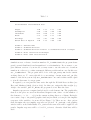
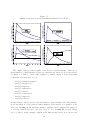
For instance, the program’s graphic output for the benchmark business cycle model
may look like Figure 5.1 and the printed output could be as presented in Table 5.1.
The number of periods considered in the computation of impulse responses is stored
in the variable nobs1. Second moments are computed as average over nofs simulations of the model, where each simulation computes times series of length nobs. The
8
Table 5.1
Second moments from simulated data:
Output
Consumption
Investment
Hours
Real Wage
Rental Rate of Capital
Column
Column
Column
Column
Column
1:
2:
3:
4:
5:
1.44
0.56
6.13
0.77
0.67
1.48
1.00
0.39
4.26
0.54
0.47
1.03
1.00
0.99
1.00
1.00
0.99
0.98
0.65
0.66
0.64
0.64
0.66
0.64
Variable name
Standard deviation
Standard deviation relative to standard deviation of Output
Cross correlation with Output
First order autocorrelation
simulations rest on draws of random numbers. If _loadShocks=0, the program draws
pseudo normal distributed random numbers for each simulation. If you want to compare different versions of your model you may want to use the same set of random
numbers in order not to confuse systematic differences with random ones. In this case
use _loadShocks=1. The program will look for a file eps_array.fmt in the current
working directory. To create this file for your settings of nobs, nofs and _nz (the
number of shocks in your model) uses _MakeShocks=1 once and set this variable equal
to 0 in all other runs of your program.
If required, you can pass the time series through the Hodrick-Prescott filter (see
Heer and Maußner (2009), Section 12.4). In this case, assign the filter weight (e.g.
1600) to the variable _HPL. If _HPL=0, the program does not filter the data.
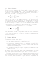
Impulse responses are computed and plotted for each element of zt . The graphic files
that store the plots are saved in files named Figure?.tkf, where ? is the number of
the element zi , i = 1, 2, . . . , n(z), in the current working directory of Gauss. Each plot
can consist of up to six panels (graphic windows) in which you can plot the impulse
responses of the variables of your model (see Figure 5.1). There are two other options
that determine the way impulse responses are plotted. If _scale=0, each graphics
window will be scaled individually. For _scale=1 the same scale will be applied to all
panels. Impulse responses will be colored if _color=1, otherwise black lines will be
used.
9
Figure 5.1
Impulse Responses from the Benchmark Business Cycle Model
The output of the program is further controlled by a Gauss structure. There are as
many instances of this structure as there are variables in your model. For each variable
for which you want to obtain either graphics or printed output your program must
contain the following lines of code:
1
2
3
4
5
6
7
8
Var[1].varname="Output";
Var[1].vartype="u";
Var[1].varpos=5;
Var[1].varprint=1;
Var[1].relsx=1;
Var[1].crosscorr=1;
Var[1].varplot=1;
Var[1].plotno=1;
In this example, Var[1] refers to the first instance of the structure Var. This instance
stores information on the variable named Output. This variable is a member of the
vector ut . In DSGE_LA the structure member vartype can be assigned the strings u,
x, l (if the variable belongs to the vector λt ), z, or y. In DSGE_QA accepted strings
are x, y, and z. In the example, output is the fifth variable in the vector u (see line
10
3). In lines 4-7, the assignment of 1 stands for true and 0 for false. Thus, varprint=1
tells the program that you want information on the second moments of the variable
output to be printed to the file specified in the variable outfile. Without any further
information the program prints the standard deviation of this variable and its first-order
autocorrelation. If you also set relsx and crosscorr to true the output table has two
additional columns that show the standard deviations of other variables relative to the
standard deviation of output and the cross-correlations of other variables with output.
In line 7 and 8 you tell the program to print the impulse response of output to the
graphics panel 1. Accepted values for plotno are the integers 1 through 6.
Finally, you may want to overwrite the program’s automatic positioning of plot
legends. In this case, you must edit the global variable _plegend. If you want to
change the lower left corner of the legend in panel i of figure j to the plot coordinates
(x, y) type
1
2
6.
_plegend[j,i,1]=x;
_plegend[j,i,2]=y;
Summary of Global Control Variables
File
Variable
Possible Settings and Effect
DSGE_LA
DSGE_LA
_GSchur
_equations
DSGE_QA
DSGE_LA/DSGE_QA
DSGE_LA/DSGE_QA
_linear
_Moments
_confidence
DSGE_LA/DSGE_QA
DSGE_LA/DSGE_QA
DSGE_LA/DSGE_QA
DSGE_LA/DSGE_QA
DSGE_LA/DSGE_QA
_IR
_nobs1
_nobs
_nofs
_HPL
DSGE_LA/DSGE_QA
DSGE_LA/DSGE_QA
DSGE_LA/DSGE_QA
_scale
_color
_LoadShocks
DSGE_LA/DSGE_QA
_MakeShocks
DSGE_LA/DSGE_QA
_outfile
1: the generalized Schur factorization will be used
1: the program expects the equations of your model in Sys1
and Sys2
1: the program computes only linear feed back rules
1: the program computes second moments
1: the program computes and prints 95 percent intervals
for the simulated moments
1: the program computes and plots impulse responses
the number of periods in each impulse response
the length of simulated time sereis
the number of simulations
the filter weight of the HP-filter, if equal to 0 the HP-filter
will not be applied
1: all graphic panels share the same scale
1: colored impulse responses are plotted
1: the program uses random numbers from the file
eps_array.fmt
1: the program draws random numbers and stores them
in the file eps_array.fmt in the current Gauss working
directory
string variable, the name of the output file
11
7.
References
Hansen, Gary D. 1985. Indivisible Labor and the Business Cycle, Journal of Monetary
Economics. Vol. 16. 309-327.
Heer, Burkhard und Alfred Maußner. 2009a. Dynamic General Equilibrium Modeling. Springer: Berlin
Heer, Burkhard und Alfred Maußner. 2009b. Computation of Business-Cycle Models with the Generalized Schur Method. Indian Growth and Development Review. Vol. 2. 173-182
12