Download CoRRAM Version 2: User Guide

CoRRAM Version 2: User Guide
Alfred Maußner
University of Augsburg
27 November 2012
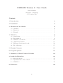
Contents
1 Introduction
2
2 Installation
2
3 Structure of the Models
3.1 Variables . . . . . . . . . . . . . . . . . . . . . . . . . . . . . . . . . . .
3.2 Equations . . . . . . . . . . . . . . . . . . . . . . . . . . . . . . . . . .
3.3 Example . . . . . . . . . . . . . . . . . . . . . . . . . . . . . . . . . . .
4
4
5
5
4 Solutions
4.1 Steady State . . . . . . . . . .
4.2 Linearization . . . . . . . . .
4.3 Structure of Solutions . . . . .
4.4 Additional Variables . . . . .
4.5 Difference Stationary Growth
4.6 Error Messages . . . . . . . .
.
.
.
.
.
.
.
.
.
.
.
.
.
.
.
.
.
.
.
.
.
.
.
.
.
.
.
.
.
.
.
.
.
.
.
.
.
.
.
.
.
.
.
.
.
.
.
.
.
.
.
.
.
.
.
.
.
.
.
.
.
.
.
.
.
.
.
.
.
.
.
.
.
.
.
.
.
.
.
.
.
.
.
.
.
.
.
.
.
.
.
.
.
.
.
.
.
.
.
.
.
.
.
.
.
.
.
.
.
.
.
.
.
.
.
.
.
.
.
.
.
.
.
.
.
.
.
.
.
.
.
.
.
.
.
.
.
.
6
7
8
13
13
14
15
5 Example Program
15
6 Program Options
21
7 Summary of Global Control Variables
22
8 Inside the Black Box
8.1 Linear Solutions . . . . . . . . . . . . . . . . . . . . . . . . . . . . . . .
8.2 Quadratic Part of the Solution . . . . . . . . . . . . . . . . . . . . . . .
8.3 Simulation . . . . . . . . . . . . . . . . . . . . . . . . . . . . . . . . . .
24
25
25
26
9 References
26
1
1
Introduction
The Gauss program CoRRAM provides a framework for computing recursive representative agent models along the lines of Heer and Maußner (2009a), Chapter 2 and Heer
and Maußner (2009b). Its aim is to allow less experienced users of Gauss to solve and
simulate their model using either linear or quadratic approximations of the model’s
equilibrium conditions.
I assume that you are familiar with dynamic stochastic general equilibrium (DSGE)
models and, in particular, with perturbation methods that obtain approximate solutions of these models. I also assume that you know how to start the Gauss software
under the Windows operating system and that you have a basic knowledge of the Gauss
syntax.
In this document I use the typewriter font to print Gauss commands and file names,
typeset vectors in boldface, and denote the number of elements in a vector x by n(x).
CoRRAM Version 2 differs from the previous version in three respects:
1. It dispenses with #include commands. The program’s functionality is provided by
Gauss procedures.
2. It includes several additional features. In particular, if you run Gauss version 12.1
or higher, you can use the new graphic capabilities of Gauss.
3. I cleaned up the code in the core, which makes the program more efficient.
2
Installation
The code of CoRRAMis stored in various files. The files with the .src and the .dec
extension contain source code that you should not change. Gauss will look for these
files in its src subdirectory. For instance, if c:\gauss is the directory where Gauss is
installed then copy the files to c:\gauss\src.
The file Tools.dll must be placed in the Gauss dlib subdirectory (for instance in
c:\Gauss\dlib). This dynamic link library contains routines written in Fortran. In
order to use this library you also have to install the file DFORRT.dll in the system32
subdirectory of your Windows 32 bit operating system (i.e. in c:\windows\system32)
or in the SysWOW64 subdirectory of your Windows 64 bit system. If you do not want
to use these routines, you can set the flag _GaussOnly=1. Yet, in this case, you will
not be able to use routines that require the generalized Schur factorization.
There are two versions of the CoRRAM Gauss library file. If you run Gauss
version 12.1 or higher copy the file CoRRAM-1.lcg to the Gauss lib directory, e.g., in
2
c:\gauss\lib and rename the file to CoRRAM.lcg. If you run Gauss version 8-12, copy
the file CoRRAM-2.lcg to the Gauss lib directory and rename it CoRRAM.lcg.
There are also two versions of a file that defines certain Gauss structures. For Gauss
versions 12.1 or higher copy CoRRAM-1.sdf to the Gauss scr directory and rename it to
CoRRAM.sdf. For Gauss versions 8-12 copy the file CoRRAM-2.sdf to src and rename
it to CoRRAM.sdf.
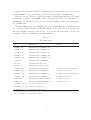
The files CoRRAM_Test_1.g, CoRRAM_Test_2.g, and CoRRAM_Test_3.g illustrate the
use of the program with the benchmark business cycle model as it is described in
Heer and Maußner (2009a), Section 2.6.1. You should run these files to check your
installation. Table 2.1 summarizes the file installation.
Table 2.1
File Installation
File
Destination
Remark
CoRRAM_1.src
[GaussDir]\src\CoRRAM_1.src
CoRRAM_2.src
[GaussDir]\src\CoRRAM_2.src
CoRRAM_3.src
[GaussDir]\src\CoRRAM_3.src
CoRRAM_4.src
[GaussDir]\src\CoRRAM_4.src
CoRRAM_5.src
[GaussDir]\src\CoRRAM_5.src
CoRRAM.dec
[GaussDir]\src\CoRRAM.dec
Plot.src
[GaussDir]\src\Plot.src
Plot-b.src
[GaussDir]\src\Plot_b.src
CoRRAM-1.sdf
[GaussDir]\src\CoRRAM.sdf
for Gauss version 12.1 and higher
CoRRAM-2.sdf
[GaussDir]\src\CoRRAM.sdf
for Gauss version 8-12
CoRRAM-1.lcg
[GaussDir]\lib\CoRRAM.lcg
for Gauss version 12.1 and higher
CoRRAM-2.lcg
[GaussDir]\lib\CoRRAM.lcg
for Gauss version 8-12
DFORRT.dll
[WinDir]\system32\DFORRT.dll
for Windows 32 bit
DFORRT.dll
[WinDir]\SysWOW64\DFORRT.dll
for Windows 64 bit
CorRRAM_Test_1.g
the users working directory
CorRRAM_Test_2.g
the users working directory
CorRRAM_Test_3.g
the users working directory
Notes: [GaussDir] refers to the directory where you have installed Gauss. [WinDir] refers to the directory
where your Windows operation system is installed.
3
3
Structure of the Models
In this section I describe the canonical form of the models that the CoRRAM-program
is able to solve. Later sections will consider different ways to input your model.
3.1
Variables
Basically, DSGE models have three different kinds of variables:
1. Purely exogenous variables, the model’s shocks,
2. state variables, i.e., endogenous variables, whose values at the beginning of time t
are predetermined (as, e.g., the stock of capital or the stock of nominal bonds),
3. endogenous variables, whose values are determined within period t.
′
I stack the shocks of period t in the column vector zt = z1t , z2t , . . . , zn(z)t . Anal
′
′
ogously, the column vectors xt = x1t , x2t , . . . , xn(x)t and yt = y1t , y2t , . . . , yn(y)t
collect the n(x) state variables and the n(y) remaining endogenous variables, respectively.
With respect to the model’s shocks, the programs assume that either their absolute or their relative deviations from their unconditional means follow the first-order
autoregressive vector process
zt = Πzt−1 + ǫt ,
(3.1a)
ǫt = σΩν t ,
(3.1b)
σ ≥ 0,
ν t ∼ N(0n(z)×1 , In(z) ).
(3.1c)
In order for this process to be stationary, the eigenvalues of the matrix Π must all be
located within the unit circle. Note that the covariance matrix Σ of the vector ǫt is
Σ = E (ǫt ǫ′t ) = E (σΩη t η ′t Ω′ σ) = σΩInz Ω′ σ = σ 2 ΩΩ′ .
Thus, if the positive definite matrix Σ rather then Ω is given and the scaling factor σ
is set equal to unity, Ω can be computed from
Ω = CΛ1/2
where
• Λ1/2 is the diagonal matrix with the square roots of the eigenvalues of the matrix
Σ on the main diagonal, and
• C is the matrix of the normalized eigenvectors of Σ so that CC ′ = In(z) .
You can use the procedure GetOmega (documented in the file CoRRAM_3.src) to obtain
Ω from Σ.
4
3.2
Equations
The dynamics of the models must be governed by the set of equations:
Et g i (xt , yt , zt , xt+1 , yt+1 , zt+1 ) = 0,
i = 1, 2, . . . , n(x) + n(y),
(3.2)
where Et denotes expectations as of period t. Usually, a subset of n(u) of the equations
will only involve date t dated variables. In this case, the dimension of the linearized
dynamic model can be reduced. Towards this purpose we partition the vector yt :
" #
ut
yt =
.
(3.3)
λt
I refer to the n(u) variables in the vector ut as control variables (this naming is borrowed
from the linear-quadratic control problem) and to the remaining variables in the n(λ)
vector λt as costate variables. Technically, the n(u) static equations determine u1t
through un(u)t for given values of the shocks zt , the state variables xt and the costate
variables λt . However, while the initial values of the variables in xt are truly given, the
initial values of the costate variables are chosen by the solution algorithm to satisfy
the model’s transversality conditions.
3.3
Example
The stationary variables of the benchmark business cycle model from Section 1.5.1
of Heer and Maußner (2009a) are the capital stock per efficiency unit, kt , output,
consumption, and investment per efficiency unit, yt , ct , and it , respectively, working
hours Nt , the rental rate of capital rt , the real wage per efficiency unit of labor wt ,
the level of total factor productivity Zt , and the scaled Lagrange multiplier of the
household’s budget constraint λt . Thus:
• xt = kt ,
• yt = [yt , ct , it , Nt , wt , rt , λt ]′ ,
• zt = ln Zt .
5
The model’s equations are:
θ(1−η)
0 = c−η
− λt ,
t (1 − Nt )
(3.4a)
0 = θc1−η
(1 − Nt )θ(1−η)−1 − λt wt ,
t
yt
0 = rt − α ,
kt
yt
0 = wt − (1 − α) ,
Nt
0 = yt − Zt Nt1−α ktα ,
(3.4b)
0 = yt − it − ct ,
(3.4f)
0 = akt+1 − (1 − δ)kt − it ,
(3.4g)
0 = λt − βa−η Et λt+1 (1 − δ + rt+1 ) ,
(3.4h)
(3.4c)
(3.4d)
(3.4e)
where a, α, β, δ, η, and θ are parameters of the model. Equations (3.4a) through (3.4f)
are static equations (i.e., they only involve variables with time index t) and, thus, 6 of
the 7 variables in the vector yt can be determined for given values of kt , Zt , and one
other variable. For instance, if we use λt as costate variable, λt ≡ λt , the vector ut
consists of yt , ct , it , Nt , wt , and rt .
Finally, with EZt = Z ≡ 1, zt := ln Zt ≃ ((Zt ) − 1)/1 evolves according to
zt+1 = ̺zt + σ Z νt+1 ,
ν ∼ N(0, 1)
so that zt ≡ zt , Π ≡ ̺, Ω ≡ 1, and σ ≡ σ Z is the standard deviation of the innovation
in the AR(1)-process of the technology shock ln Zt .
4
Solutions
Note that for σ = 0 the model in (3.1) and (3.2) collapses to a deterministic model, in
which all shocks equal their conditional means of zero. Given that the deterministic
model is stable, it will approach a stationary solution (or a balanced growth path) in
which all variables remain constant. The CoRRAM program computes linear and
quadratic approximations of the stochastic model’s solution at this point.
There are two ways to compute the quadratic part. If the global control variable
_QA_type is set to zero, the code is based on Heer and Maußner (2009a), pp. 124-131.
If this variable is set to one, the algorithm of Gomme and Klein (2011) is employed. In
this case, the global control variable _sylvester determines if the respective Sylvester
equation is solved by applying the vec operator or by a call to a routine stored in
Tools.dll. The default settings of _QA_type and _sylvester are 1.
Both the linear and the quadratic approximations build on the linearized equations
(3.2). In order to understand the way you can input your model and to be able to
6
respond to error messages reported by the program you need a basic understanding of
the linearized model.
4.1
Steady State
The stationary solution is obtained from (3.2) in the following steps:
1. Replace zt by its unconditional mean z = 0 so that the expectations operator Et
can be ignored.
2. Assume stationarity, i.e., drop the time index from all variables.
3. Solve
g i (x, y, z, x, y, z) = 0,
i = 1, 2, . . . , n(x) + n(y),
for x and y.
There are two ways to compute this solution: a) Use paper and pencil to reduce
the system so that it can be solved equation by equation, and b) employ a non-linear
equations solver.
Step by Step. Consider example (3.4). In the steady state with Z ≡ 1 it reduces
to:
0 = c−η (1 − N)θ(1−η) − λ,
(4.1a)
0 = θc1−η (1 − N)θ(1−η)−1 − λw,
y
0=r−α ,
k
y
0 = w − (1 − α) ,
N
1−α α
0 =y−N
k ,
(4.1b)
(4.1c)
(4.1d)
(4.1e)
0 = y − i − c,
(4.1f)
0 = ak − (1 − δ)k − i,
(4.1g)
−η
0 = λ − βa λ (1 − δ + r) .
(4.1h)
Substituting equation (4.1c) into (4.1h) we can solve for the output-capital ratio:
aη − β(1 − δ)
y
=
.
k
αβ
(4.2a)
The resource constraint (4.1f) and equation (4.1g) imply
c
y
= − (a − 1 + δ).
k
k
(4.2b)
7
Substituting for λ in (4.1b) from (4.1a) and for w from (4.1d) yields:
N
1−αy
=
1−N
θ c
(4.2c)
which can be solved for N, since y/c = (y/k)/(c/k). The production function (4.1e)
implies
1
k
= (y/k) α−1 .
N
(4.2d)
Thus, given the solution for N we can back out the stationary values of k, y, c. Given
these, equations (4.1a), (4.1c), and (4.1d) can be used to determine λ, r, and w,
respectively.
Simultaneously. Instead of solving (4.1) stepwise you may want to input the system
in Gauss and use either the Gauss command EqSolve or any other program that solves
a system of non-linear equations. The Gauss non-linear equations solver needs an
initial vector x0 = [k0 , y0 , c0 , i0 , N0 , w0, r0 , λ0 ]′ to start the algorithm. If you do not
have prior knowledge of the solution, you can use random numbers distributed on a
positive subset of R8 . However, since solving non-linear equations is sometimes a tricky
business, there is no guarantee that this approach works in all situations.
Given that you have managed to find the stationary solution of the model, you can
proceed to give the program the information from which it will compute the linearized
model.
4.2
Linearization
The CoRRAM program has two options that are chosen by the flag _equations.
• _equations=1: numeric differentiation will be used,
• _equations=0: you must provide the coefficient matrices of the log-linearized
system.
However, since the quadratic part of the solution always rests on second derivatives of
the system (3.2), the option _equations=0 restricts you to linear approximate solutions. In addition, the option _GSchur=1 cannot be used. I will provide further details
below.
8
Via Numeric Differentiation. Internally, the program uses two different representations of the linearized model. If the flag GSchur is set to 1 (i.e., to true), the program
computes
"
#
" #
¯ t+1
¯t
x
x
BEt
=A
+ Czt ,
(4.3)
¯ t+1
¯t
y
y
¯t ≡
where the bar denotes (absolute) deviations from the stationary solution, i.e., x
1
xt − x and so forth. The matrices B, A, and C are derived from the derivatives of
g i (x1 , y1 , z1 , x2 , y2 , z2 ),
i = 1, 2, . . . , n(x) + n(y)
(4.4)
with respect to current period variables (superscript 1) and next period variables (superscript 2) evaluated at the stationary solution. If some of the model’s equations
involve only current period values, the matrix B will be singular. The generalized
Schur factorization (see Heer and Maußner (2009b)) is applied to find a linear approximate solution.
If GSchur=0 the program reduces the dynamic linearized system to a smaller one.
Toward this purpose it must know the number of static equations, which you must
supply in the scalar _nu. First, the program computes the matrices of the system:
" #
¯t
x
¯ t = Cxλ
Cu u
+ C z zt ,
(4.5a)
¯t
λ
"
#
" #
¯ t+1
¯t
x
x
¯ t+1 + Fu u
¯ t + Dz Et zt+1 + Fz zt ,
Dxλ Et
+ Fxλ
= Du Et u
(4.5b)
¯ t+1
¯t
λ
λ
Second, it reduces this system to
"
#
" #
¯ t+1
¯t
x
x
Et
= B −1 A
+ B −1 Czt ,
¯
¯
λt+1
λt
(4.6)
where
B := Dxλ − Du Cu−1 Cxλ ,
A := − Fxλ − Fu Cu−1 Cxλ ,
C := Dz + Du Cu−1 Cz Π + Fz + Fu Cu−1 Cz .
This system is solved for the linear part of the solution by applying the Schur factorization to the matrix B −1 A. Error messages may occur:
• if the matrix Cu is singular,
1
Since the stationary value of the vector zt is the zero vector, ¯zt ≡ zt .
9
• if the matrix B is singular.
The first error message will occur, if the ordering of your variables in the vector yt is
unfortunate. The program partitions the vector yt (see (3.3)) by assigning the first
_nu variables to the vector ut and the remaining n(y) − n(u) variables to the vector λt .
Now, suppose that one of your static equations only involves variables from the vectors
xt and λt . In this case, the respective line of Cu has zero elements and the matrix,
thus, is singular. By changing the ordering of the variables, you can work around this
problem.
The second error message will occur, if more than n(u) of the linearized equations are
static. This will happen, if some of the linearized dynamic equations can be arranged
to imply a further static equation. If you are not able to figure this out and change
the system accordingly, use GSchur=1.
In order to compute the matrices in either (4.3) or (4.5), you must supply the
equations in a procedure named Sys. This procedure receives the vector
w = [x1 , y1 , z1 , x2 , y2 , z2 ]′
and returns the right-hand side of (4.4). If GSchur=0 the program assumes that the
first _nu equations in Sys are static equations.
As an example of Sys consider the system (3.4).
1
proc(1)=Sys(w);
2
3
4
5
6
7
8
9
10
11
12
13
local fx, c1, y1, i1, r1,w1,n1, k1, l1, z1,
c2, y2, i2, r2,w2,n2, k2, l2, z2;
k1=w[1];
y1=w[2];
c1=w[3];
i1=w[4];
r1=w[5];
w1=w[6];
n1=w[7];
l1=w[8];
z1=exp(w[9]);
14
15
16
17
18
19
20
21
k2=w[10];
y2=w[11];
c2=w[12];
i2=w[13];
r2=w[14];
w2=w[15];
n2=w[16];
10
22
23
l2=w[17];
z2=exp(w[18]);
24
25
fx=zeros(_nx+_ny,1);
26
27
28
29
30
31
32
fx[1]=(c1^(-eta))*((1-n1)^(theta*(1-eta)))-l1;
fx[2]=theta*(c1^(1-eta))*((1-n1)^(theta*(1-eta)-1))-w1*l1;
fx[3]=w1-(1-alpha)*z1*(n1^(-alpha))*(k1^alpha);
fx[4]=r1-alpha*z1*(n1^(1-alpha))*(k1^(alpha-1));
fx[5]=y1-z1*(n1^(1-alpha))*(k1^alpha);
fx[6]=y1-c1-i1;
33
34
35
fx[7]=a*k2-(1-delta)*k1 - i1;
fx[8]=beta*(a^(-eta))*l2*(1-delta+r2)-l1;
36
37
38
if _eqno==0; retp(fx); else; retp(fx[_eqno]); endif;
retp(fx);
39
40
endp;
In lines 5-23 the variables in the vector w are written in scalar variables with obvious
notation. This makes it easier to write the equations. Of course, you can use w[1]w[17] instead of the auxiliary variables. The code in lines 27-32 evaluates the static
functions (3.4a)-(3.4f) and stores the respective results in the vector fx. Lines 34 and
35 relate to the dynamic equations (3.4g) and (3.4h). Line 38 returns the vector fx
to the calling program. The code in line 37 is required to compute second derivatives
(which is done equation by equation) and must not be changed!
Linearization by Paper and Pencil. Numeric derivatives cannot be as precise as
analytical ones. In addition, by writing the linearized model in terms of percentage
instead of absolute deviations, the coefficient matrices usually involve only elasticities
so that the numeric differences between their elements are small making matrix factorization less imprecise. Furthermore, it is often not necessary to derive the stationary
solutions of all variables.
Consider the benchmark model of (3.4). Its linearized version is an example of:
" #
ˆt
x
ˆ t = Cxλ
Cu u
+ Cz ˆzt ,
(4.7a)
ˆt
λ
"
" #
#
ˆ t+1
ˆt
x
x
ˆ t+1 + Fu u
ˆ t + Dz Et zˆt+1 + Fz ˆzt ,
(4.7b)
Dxλ Et
+ Fxλ
= Du Et u
ˆ t+1
ˆt
λ
λ
zˆt = Πˆzt−1 + σΩν t , ν t ∼ N(0n(z)×1 , In(z) ),
11
(4.7c)
where the hat denotes relative deviations from the stationary solution, i.e., xˆt ≡ (xt −
x)/x for any variable x of the model including the shocks. The vectors and matrices
are:
ˆt ≡ λ
ˆ t , ˆzt ≡ Zˆt ,
ˆt , wˆt , rˆt ]′ , x
ˆ t ≡ [ˆ
ˆ t ≡ kˆt , λ
u
yt , cˆt , ˆit , N


N
0
−η
0
−θ(1 − η) 1−N
0 0
 0 (1 − η) 0 −[θ(1 − η) − 1] N −1 0


1−N


−1
0
0
0
0 1

,
Cu = 

−1
0
0
1
1
0




1
0
0
α−1
0 0
− yi
0
0 0
1
− yc

 

0 1
0

 

 0 1
0
"
#
"
#

 

−1 0
0
δ
−
1
0
a
0
 

Cxλ = 
,
 0 0 , Cz = 0 , Dxλ = 0 1 , Fxλ =
0
−1

 


 

 α 0
1
0 0
0
"
#
0 0 0 0 0
0
Du =
,
0 0 0 0 0 βa−η (1 − δ) − 1
"
#
0 0 a−1+δ 0 0 0
Fu =
,
0 0
0
0 0 0
" #
0
Dz = Fz =
.
0
If you set _equations=0, you must input the matrices Cu, Cxl, Cz, Dxl, Fxl, Du,
Fu, Dz and Fz. Also note that in this case the program assumes that the percentage
(and not the absolute) deviations of the shock variables are governed by the first-order
vector autoregressive process (4.7c).
As in the case of (4.5), the system (4.7) is reduced to the smaller dynamical system
"
#
" #
ˆ t+1
ˆt
x
x
Et
= B −1 A
+ B −1 Cˆzt ,
ˆ
ˆ
λt+1
λt
(4.8)
B := Dxλ − Du Cu−1 Cxλ ,
A := − Fxλ − Fu Cu−1 Cxλ ,
C := Dz + Du Cu−1 Cz Π + Fz + Fu Cu−1 Cz .
Thus, you will observe error messages if either Cu or B are not invertible.2 In this
2
The solution algorithm does not use matrix inversion but solves the respective linear systems.
Yet, it checks whether Cu and B are singular before trying to solve theses systems.
12
case you must check your derivation of the model for mistakes or your model input for
typing errors.
4.3
Structure of Solutions
The approximate solutions of a DSGE model are feed-back rules that determine the
model’s endogenous variables xt+1 and yt as linear or quadratic functions of the model’s
current states xt and realizations of the shocks zt .
If _equations=0 the program computes the four matrices that govern the approximate dynamic solution
ˆ t+1 = Lxx x
ˆ t + Lxz ˆzt ,
x
(4.9a)
ˆ t = Lyx x
ˆ t + Lyz zˆt .
y
(4.9b)
If _equations=1 and linear=0 the solutions are:
 
¯t
x
i
1h ′
i ′
i ′
i 
′
¯ t + (lz ) ¯zt +
= xi + (lx ) x
¯ , zt , σ H  zt  , i = 1, . . . , n(x),
x
2 t
σ
(4.10a)
 
¯t
x
h
i
1 ′


j
j ′
j ′
¯ t + (lz ) z¯t +
yjt = yj + (lx ) x
¯ t , z′t , σ H  zt  , j = 1, . . . , n(y).
x
2
σ
(4.10b)
xit+1
If _linear=1 the program returns only the linear part of this solution.
4.4
Additional Variables
Occasionally you may want solutions for variables that cannot be included in yt , since
they depend on the model’s solution. For instance, in the benchmark model the current
price pt of a bond that pays one unit of consumption for certain in the next period is
given by
pt = βa−η Et
λt+1
,
λt
so that
ˆ t+1 − λ
ˆt.
pˆt = Et λ
From the linear solution (where lλx denotes the row of Lyx that refers to the coefficients
of the solution for λ)
ˆ t = (lλ )′ xˆt + (lλ )′ zˆt
λ
x
z
13
you get
ˆ t+1 = Et (lλ )′ xˆt+1 + (lλ )′ zˆt+1 ,
Et λ
x
z
= (lλx )′ {Lxx xˆt + Lxz zˆt } + (lλz )′ Et {Πˆ
zt + ǫt+1 } ,
= (lλx )′ Lxx xˆt + ((lλx )′ Lxz + (lλz )′ Π zˆt .
Therefore, you can determine pˆt as a linear function of xˆt and zˆt with matrices:3
Lsx = (lλx )′ (Lxx − In(x) ),
(4.11)
Lsz = (lλx )′ Lxz + (lλz )′ (Π − In(z) ).
Note that the program must compute the linear solution before it can determine Lsx
and Lsz . For this reason you must input the two matrices before your simulate the
model. Also, you must set the scalar _ns to the number of additional variables and
position these variables in the vector y to the right of the model’s original variables.
Note also that this opportunity is available to you in the case _equations=0 only!
4.5
Difference Stationary Growth
The computation of impulse responses and second moments depends on the interpretation of the model’s variables. In the model of equations (3.4) the variables are scaled
by the level of labor augmenting technical progress At which growth deterministically
at the rate a − 1. Many DSGE models, however, assume that At grows according to
the law
at =
At+1
,
At
(4.12)
at = eln a+ln zt ,
ln zt = ρ ln zt−1 + σǫt ,
ǫt ∼ N(0, 1),
so that ln At is a difference stationary growth process. In this case, the program assumes
that you have defined stationary variables according to Xt = xt Aξt−1 , where Xt is the
level of a variable, xt is the solution for the scaled variable computed by the program,
and the exponent ξ is either zero (if the variable needs not to be scaled, as for instance
hours Nt ), equal to ξ = 1 (if division by At−1 makes a variable stationary), or equal
to ξ = η, as in the case of the Lagrange multiplier in the benchmark business cycle
model, where η is coefficient of relative risk aversion.
3
The program uses the matrices Lsx and Lsz to denote the relation between the additional variables
ˆ t and ˆzt . In this one variable example, Lsx and Lsz are row
in the subvector s and the variables in x
vectors.
14
To get the correct interpretation of impulse responses and second moments4 you
must
• set the flag _DS=1,
• provide information on ξ in the structure _Var (see below),
• use the variable at as the first element in the vector yt .
4.6
Error Messages
DSGE models have determinate solutions if:
• n(x) of the eigenvalues of B −1 A or n(x) of the eigenvalues of the matrix pencil
(B, A) are inside the unit circle, and
• n(λ) of the eigenvalues B −1 A or n(y) of the eigenvalues of the matrix pencil
(B, A) are outside of the unit circle.
The program stops with an error message if these two conditions are not satisfied or if
it is not able to factorize either B −1 A or (B, A). The latter usually points to errors in
your code.
When the program computes the linear part of the solution it uses complex arithmetic. If the matrices of your model are large and/or rather unbalanced, roundoff
errors may cause the complex part of the solution matrices to be non-negligible. If
this happens, the program issues a warning message. Please check if errors in your
code cause this problem or if changing the matrix factorization method (see above, the
setting of GSchur) solves the problem.
5
Example Program
This section explains the code in the file CoRRAM_Test_2.g which solves and simulates
the model of (3.4) using the model’s equations.
1
@ ----------- CoRRAM_Test_3.g ------------------------
2
3
4
Alfred Maußner
17 September 2012
5
6
Purpose: Solve the benchmark business cycle model
4
See Appendix C of Heer and Maußner (2010) for the computation of impulse responses in such a
model.
15
7
8
of Heer and Maußner (2009) using the
CoRRAM toolbox.
9
10
------------------------------------------------------ @
11
12
13
14
15
// Do not change the next there lines of code:
new;
library user, pgraph, corram;
#include CoRRAM.sdf;
16
17
18
19
20
21
22
23
nx=1;
ny=7;
nu=6;
nz=1;
ns=0;
_PQG=1;
_loadShocks=1;
24
25
NewModel("Benchmark-1.txt",nx,ny,nu,nz,ns);
26
27
28
29
30
31
32
33
34
_Var[1].name="Output";
_Var[1].type="y";
_Var[1].pos=1;
_Var[1].print=1;
_Var[1].crosscorr=1;
_Var[1].plot=1;
_Var[1].plotno=2;
_Var[1].relsx=1;
35
36
37
38
39
40
41
42
_Var[2].name="Consumption";
_Var[2].type="y";
_Var[2].pos=2;
_Var[2].print=1;
_Var[2].crosscorr=0;
_Var[2].plot=1;
_Var[2].plotno=2;
43
44
45
46
47
48
49
50
_Var[3].name="Investment";
_Var[3].type="y";
_Var[3].pos=3;
_Var[3].print=1;
_Var[3].crosscorr=0;
_Var[3].plot=1;
_Var[3].plotno=2;
51
16
52
53
54
55
56
57
58
_Var[4].name="Hours";
_Var[4].type="y";
_Var[4].pos=4;
_Var[4].print=1;
_Var[4].crosscorr=0;
_Var[4].plot=1;
_Var[4].plotno=2;
59
60
61
62
63
64
65
66
_Var[5].name="Real Wage";
_Var[5].type="y";
_Var[5].pos=5;
_Var[5].print=1;
_Var[5].crosscorr=1;
_Var[5].plot=1;
_Var[5].plotno=3;
67
68
69
70
71
72
73
74
_Var[6].name="User Costs of Capital";
_Var[6].type="y";
_Var[6].pos=6;
_Var[6].print=1;
_Var[6].crosscorr=0;
_Var[6].plot=1;
_Var[6].plotno=3;
75
76
77
78
79
80
81
82
_Var[7].name="Marginal Utility";
_Var[7].type="y";
_Var[7].pos=7;
_Var[7].print=1;
_Var[7].crosscorr=0;
_Var[7].plot=1;
_Var[7].plotno=3;
83
84
85
86
87
88
89
90
_Var[8].name="Capital Stock";
_Var[8].type="x";
_Var[8].pos=1;
_Var[8].print=0;
_Var[8].crosscorr=0;
_Var[8].plot=1;
_Var[8].plotno=4;
91
92
93
94
95
96
_Var[9].name="TFP Shock";
_Var[9].type="z";
_Var[9].pos=1;
_Var[9].print=0;
_Var[9].crosscorr=0;
17
97
98
_Var[9].plot=1;
_Var[9].plotno=1;
99
100
101
102
/* Set legend positions individually */
_plegend[1,1,1]=10;
_plegend[1,1,2]=0.5;
103
104
105
_plegend[1,2,1]=10;
_plegend[1,2,2]=3.5;
106
107
108
_plegend[1,4,1]=6;
_plegend[1,4,2]=0.5;
109
110
111
112
113
114
115
116
117
118
// The parameter of the model
a=1.005;
alpha=0.27;
beta=0.994;
eta=2.0;
delta=0.011;
rhoZ=0.90;
sigmaz=0.0072;
nstar=0.13;
119
120
121
122
_Rho[1,1]=RhoZ;
_Omega[1,1]=SigmaZ;
_Sigma=1;
123
124
125
126
127
128
129
130
131
132
133
134
135
// Compute the stationary solution
yk=(a^eta-beta*(1-delta))/(beta*alpha);
ck=yk+(1-a-delta);
theta = (1-alpha)*(yk/ck)*(1-nstar)*(1/nstar);
kn=yk^(1/(alpha-1));
kstar=kn*nstar;
ystar=yk*kstar;
cstar=ck*kstar;
istar=ystar-cstar;
wstar=(1-alpha)*(ystar/nstar);
rstar=alpha*yk;
lstar=(cstar^(-eta))*((1-nstar)^(theta*(1-eta)));
136
137
138
139
140
141
// assign the stationary values
_var[1].star=ystar;
_var[2].star=cstar;
_var[3].star=istar;
_var[4].star=nstar;
18
142
143
144
145
146
_var[5].star=wstar;
_var[6].star=rstar;
_var[7].star=lstar;
_var[8].star=kstar;
_var[9].star=0;
147
148
149
// solve the model
retc=SolveModel;
150
151
152
153
154
// simulate the model
if retc;
SimulateModel(25,80,500);
endif;
155
156
ende:
157
158
end;
159
The file header in lines 1-10 provides information on the author of the program, the
date at which the program was written, and the purpose of the program. Lines 13-15
must be present in each program. The new command clears the Gauss memory. The
command in line 14 loads the Gauss libraries required by the program. These provide
information to Gauss where the CoRRAM procedures are stored. The command in
line 15 loads the definitions of several Gauss structures that are used by CoRRAM.
Lines 17-21 provide information on the number of variables. In lines 22 and 24 two
of the default options are changed. The option _LoadShocks=1 instructs the program
to load the random numbers used to simulate the model from a file. Depending on
the flag _GLight this file has the extension .fmt (_Glight=0) or .xls (_Glight=1).
You will get an error message if this file is not present in the current working directory.
You can create this file with the command MakeShocks(nz,nobs,nofs) (place it before
the command SimulateModel or issue this command from the command prompt.) nz,
nobs, and nofs refer to the number of shock, the length of the simulated time series,
and the number of simulations, respectively.
The command in line 25 sets up a new model. Output (including error messages)
will be directed to the file Benchmark-1.txt in the current working directory.
The code in lines 27-98 provides CoRRAM with information on the variables
(names, types,positions,stationary values,scaling,print and output options) which I will
explain below in more detail.
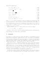
In lines 104-108 the legends in the Gauss publication quality graphics are repositioned (see below). The statements in lines 111-118 assign values to the parameters of
19
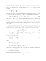
Figure 5.1
Impulse Responses from the Benchmark Business Cycle Model
the model. The code in lines 120-122 provides CoRRAM with information about the
matrices Π (_Rho in CoRRAM) and Ω.
Lines 125-146 compute and assign the stationary values of the variables. The statement in line 149 solves the model, i.e., it computes either the linear or quadratic
approximate solution. The procedure SolveModel returns retc=1 if the model could
be solved and zero otherwise.
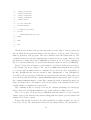
The statement in line 153 computes impulse responses and second moments. The
number of periods for which impulse responses are computed is given in nobs1. If
this is set equal to zero, the program does not compute and plot impulse responses.
Depending on the flag _PQG, the program will plot the impulse responses either with the
Gauss publication quality graphic routines (_PQG=1) or with the new graphic routines
implemented since Gauss version 12.1. For instance, the program’s graphic output for
the benchmark business cycle model may look like Figure 5.1
There are two other options that determine the way impulse responses are plotted.
If _scale=0, each graphics window will be scaled individually. This option does not
20
work under _PQG=0. For _scale=1 the same scale will be applied to all panels. Impulse
responses will be colored if _color=1, otherwise black lines will be used.
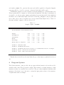
CoRRAM computes second moments from nofs simulations of length nobs2 each.
The program will not compute second moments if nobs2=0. If the flag _confidence is
set equal to one, the program computes and prints 95 percent intervals for the simulated
moments. If you run Gauss Light, and have set the flag _GLight=1, the program will
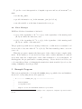
ignore this option, since it requires more storage than Gauss Light allows. Table 5.1
presents example output for the model in (3.4).
Table 5.1
Sample output of CoRRAM
Second moments from simulated data:
Output
Consumption
Investment
Hours
Real Wage
Rental Rate of Capital
Column
Column
Column
Column
Column
1:
2:
3:
4:
5:
1.44
0.56
6.13
0.77
0.67
1.48
1.00
0.39
4.26
0.54
0.47
1.03
1.00
0.99
1.00
1.00
0.99
0.98
0.65
0.66
0.64
0.64
0.66
0.64
Variable name
Standard deviation
Standard deviation relative to standard deviation of Output
Cross correlation with Output
first order autocorrelation
Finally, lines 160-201 (not shown) define the procedure Sys as explained in Section
4.2.
6
Program Options
The Gauss structure _Var provides the program with information about the model’s
variables and controls the program’s output. There must be as many instances of this
structure as there are variables in your model. The procedure NewModel initializes this
structure. It is then to up to the user to assign the appropriate values to the structure.
I explain this with an example.
21
1
2
3
4
5
6
7
8
9
10
_Var[1].name="Output";
_Var[1].type="y";
_Var[1].pos=1;
_Var[1].print=1;
_Var[1].relsx=1;
_Var[1].crosscorr=1;
_Var[1].plot=1;
_Var[1].plotno=1;
_Var[1].star=ystar;
_Var[1].xi=1;
_Var[1] refers to the first instance of the structure _Var. This instance stores
information on the variable named Output. This variable is a member of the vector yt .
The structure member type can be assigned the strings x, y, and z, depending on to
which vector of variables it belongs. In the example, output is the first variable in the
vector y (see line 3). In lines 4-7, the assignment of 1 stands for true and 0 for false.
Thus, print=1 tells the program that you want information on the second moments
of the variable output to be printed. Without any further information the program
prints the standard deviation of this variable and its first-order autocorrelation. If you
also set relsx and crosscorr to true, the output table has two additional columns
that show the standard deviations of other variables relative to the standard deviation
of output and the cross-correlations of other variables with output.
In line 7 and 8 you tell the program to print the impulse response of output to the
graphics panel 1. Accepted values for plotno are the integers 1 through 6. Finally,
you may want to overwrite the program’s automatic positioning of plot legends. In
this case, you must edit the global variable _plegend. If you want to change the lower
left corner of the legend in panel i of figure j to the plot coordinates (x, y), type
1
2
_plegend[j,i,1]=x;
_plegend[j,i,2]=y;
Note, this works only if _PQG=1. For _PQG=0 you must position the legend box manually
in the Gauss graphics tab.
7
Summary of Global Control Variables
Table 7.1 explains the settings of the variables that determine the solution method and
the output options of CoRRAM.
22
Table 7.1
Global Control Variables of CoRRAM
Variable
Possible Settings and Effect
_color
_confidence
1
0
1
_DS
0
1
0
_GaussOnly
1
0
1
_Glight
0
1
_equations
0
_GSchur
1
0
_HPL
0
_plegend
_LoadShocks
1
0
1
_PQG
0
1
_linear
0
_QA_type
_scale
_Sylvester
1
0
1
0
1
0
Default
colored impulse responses are plotted
all impulse responses are black.
the program prints 95 percent intervals for the computed second moments
the program prints only averages of the second moments
the program assumes a difference stationary growth process. The
variable at must be the first element in the vector yt .
the program assumes that the variables in your model are stationary,
either since there is no growth or since the growth process is deterministic.
the program expects the equations of your model in Sys
you must input the coefficient matrices of the log-linearized model
no foreign language code will be loaded, the generalized Schur factorization is then not available.
Fortran routines from Tools.dll will be used.
if _LoadShocks=1 random numbers will be read from an Excel spreadsheet which you can create with the procedure MakeShocks.
if _LoadShcoks=1 random numbers will be read from a Gauss matrix
file. In addition, you may use the flag _confidenc=1.
the generalized Schur factorization will be used
the Schur factorization will be used
the filter weight of the HP-filter
the HP-filter will not be applied
three dimensional array that stores information on the individual positioning of legends.
the program computes only linear feed back rules
the program computes quadratic feed back rules
the program uses random numbers from the file eps_array.fmt or
eps_array.xls
the program generates new random numbers for each simulation.
impulse responses will be plotted using publication quality graphic
commands.
impulse responses will be plotted using the new (since Gauss version
12.1) plotXY command.
second order solution is based on the chain rule for Hessian matrices
second order solution is based on tensor products
all graphic panels share the same scale
all graphic panels will be scaled individually.
if _QA_type=1 the routine sylvester in Tools.dll is used
if _QA_type=1 the vec operator is used
1
0
0
1
0
0
0
1600
0
0
1
1
1
1
Besides the control variables there are a number of other global variables used by the
program. All global variables begin with an underscore _. Please do not use variable
names that begin with an underscore. This avoids that you interfere with the program
code. Table 7.2 displays variables used by CoRRAM. Please adhere to these naming
conventions.
23
Table 7.2
Symbol Table
8
Symbol Name
Equivalent Symbol or Function
_Cu
_Cxl
_Cz
_Dxl
_Fxl
_Du
_Fu
_Dz
_Fz
_sigma
_Omega
_Rho
_nx
_ny
_nz
_ns
_nu
_xstar
_ystar
_wstar
_xt
_yt
_zt
Sys
_Lxx
_Lxz
_Lyx
_Lyz
_Lsx
_Lsz
_xcube
_ycube
Cu from (4.7a)
Cxλ from (4.7a)
Cz from (4.7a)
Dxλ from (4.7b)
Fxλ from (4.7b)
Du from (4.7b)
Fu from (4.7b)
Dz from (4.7b)
Fz from (4.7b)
σ from (3.1b) or (4.7c)
Ω from (3.1b) or (4.7c)
Π from (3.1b) or (4.7c)
n(x) the number of variables in the vector xt
n(y) the number of variables in the vector yt
n(z) the number of variables in the vector zt
the number of additional variables (see Section 4.4)
the number of static equations
the vector with the stationary solutions of the state variables
the vector with the stationary solutions of the non predetermined variables
the vector _xstar|_ystar|_zstar
three dimensional array that stores the impulse responses of the variables in xt .
three dimensional array that stores the impulse responses of the variables in yt .
three dimensional array that stores the impulses from zt .
the procedure with the model’s equations from (3.2)
Lx
x from (4.9)
Lx
z from (4.9)
Lyx from (4.9)
Lyz from (4.9)
Lsx from (4.11)
Lsz from (4.11)
three dimensional array, page j stores H j from (4.10a)
three dimensional array, page j stores H j from (4.10b)
Inside the Black Box
If the standard options provided to you via the command NewModel, SolveModel, and
SimulateModel satisfy your needs, you can skip this section and start right away with
setting up your own model or run CoRRAM_Test_1.g and CoRRAM_Test_2.g. Otherwise,
the information in this section will help you to use the main procedures that make up
CoRRAM.
24
8.1
Linear Solutions
If you do not input the matrices from the system (4.7), the code in the procedure
SolveModel in the file CoRRAM_1.src sets up the matrices from which the linear
part of the solution will be computed. If _GSchur=0 (the default), the procedure
SolveReducedModel builds the model in (4.6) and solves it with a call to SolveLA1 (in
CoRRAM_4.src), otherwise SolveModel builds the model in (4.3) and solves it with a
call to SolveLA2 (also in the file CoRRAM_4.src). Depending on the flag _GaussOnly,
the procedure SolveLA1 either uses Gauss commands to compute the Schur factorization of the matrix B −1 A or calls a procedure in the dynamic link library Tools.dll to
get the factorization. The option GSchur=1 always calls a procedure in Tools.dll since
Gauss provides no command to compute the generalized Schur factorization. When
SolveModel is finished, the matrices _Lxx, _Lxz, _Lyx, and _Lyz store the solution
matrices from (4.9).
8.2
Quadratic Part of the Solution
Given the linear part of the solution, either the program SolveQA2 or the program
SolveQA3 (both in the file CoRRAM_5.src) computes two three dimensional arrays that
store the matrices H i and H j from (4.10). The respective call is:
{_xcube,_ycube}=SolveQA2(_Lxx,_Lxz,_Lyx,_Lyz,_gmat,hcube);
or
{_xcube,_ycube}=SolveQA3(_Lxx,_Lxz,_Lyx,_Lyz,_gmat,hcube);
If the global control variable _QA_type is true (i.e. set equal to one, the default setting)
SolveQA2 is used.
The matrix _gmat stores the Jacobian matrix of the system (4.4), and the three
dimensional array hcube holds the Hesse matrices of the individual equations g i (·)
of (4.4). They are computed by CDJac and CDHesse, which employ central difference
formulas to approximate first and second derivatives, respectively. Each page of _xcube
stores one of the n(x) matrices H i of (4.10a). Analogously, the n(y) pages of _ycube
store the matrices H j of (4.10b). The procedure PF uses _Lxx, _Lxz, _Lyx, _Lyz,
¯ t and z¯t , so that you can
_xcube, and _ycube and returns xit+1 and ytj as functions of x
use this procedure to simulate your model. The respective call is:
xi = PF("x",i,whut),
yj = PF("y",j,whut),
where i and j refer to the position number (starting from the left) of xi and yj in the
vectors xt and yt , respectively. The vector whut stores wt := [¯
x′t , ¯z′t , σ]′ .
25
8.3
Simulation
The procedures Impulse1 and Impulse2 compute the impulse responses. Impulse1
is invoked, if _equations=0. Both procedures return the percentage deviations of the
model’s variables in the matrices xt, yt, and zt. Each row of these matrices stores
nobs1 elements of the response of the respective variable to a one-standard deviation
shock νl2 = σΩel , where el is the row vector with its l-th element equal to one and
zeros elsewhere. The impulse response of the state variables are stored in xt, those of
the non-predetermined variables in yt, and those of the shocks in zt. The program
computes as many impulse responses as are elements in the vector zt . They are stored in
three arrays, _xt, _yt, and _zt, respectively. Page i refers to shock i ∈ {1, 2, . . . , n(z)}.
The order of the variables in the columns of each page confirms to the numbering of the
variables specified in the structure _Var. When the program is finished, these arrays
stay in the Gauss memory until a new version of the program is run or the Gauss
window is closed.
Analogously, the procedures RBCRun1 and RBCRun2 simulate the model for ongoing
shocks. If _confidence=0 they return a vector sx and a matrix rx. The vector sx stores
the standard deviations (in percent) of the variables. The first n(x) elements refer to
the state variables, the second n(y) elements refer to the non-predetermined variables
and third n(z) elements relate to model’s shocks. The matrix sx has dimension 2n×2n,
n = n(x) + n(y) + n(z). Its first n × n block stores the contemporaneous correlation
between the elements of the vector
′
vt = x1t , . . . , xn(x)t , y1t , . . . , yn(y)t , z1t , . . . , zn(z)t .
The block with elements sxij , i = 1, . . . , n, j = n+1, . . . , 2n, holds the cross-correlations
between the elements of vt and vt−1 .
If _confidence=1, sx is a matrix. Column i of this matrix stores the standard
deviations of the elements of the vector [x, y, z]′ from the i-th simulation of the model.
Analogously, rx is a three dimensional array, where the i-th page stores the contemporaneous and one-period lagged correlations between the model’s variables.
9
References
Gomme, Paul and Paul Klein. 2011. Second-Order Approximation of Dynamic Models
Without the Use of Tensors. Journal of Economic Dynamics & Control. Vol. 35.
604-615.
Hansen, Gary D. 1985. Indivisible Labor and the Business Cycle, Journal of Monetary
Economics. Vol. 16. 309-327.
26
Heer, Burkhard und Alfred Maußner. 2009a. Dynamic General Equilibrium Modeling. Springer: Berlin
Heer, Burkhard und Alfred Maußner. 2009b. Computation of Business-Cycle Models with the Generalized Schur Method. Indian Growth and Development Review. Vol. 2. 173-182
Heer, Burkhard and Alfred Maußner. 2010. Inflation and Output Dynamics in a Model
with Labor Market Search and Capital Accumulation. Review of Economic Dynamics. Vol. 13. pp. 654-686.
27