Download LLBo Applets User Guide - Lehrstuhl für Leichtbau

Technische Universität München
Aerospace Department
Institute of Lightweight Structures
Univ. Prof. Dr.-Ing. Horst Baier
LLBo Applets User Guide
Author:
Supervisor:
Date:
Alexei Perro B.Sc.
Erich Wehrle M.Sc.
September 9, 2010
Abstract:
Application of concepts introduced in the course Multidisciplinary Design Optimization often
requires skills that cannot be acquired from theoretical studies only. This set of interactive
applets is meant to illustrate the most fundamental notions in a hands-on way. This guide can
serve as a reference while using those applets and also provides some theoretical background
on relevant topics.
Keywords:
Minimization, constrained optimization, finite differencing, feasible directions, SUMT, KuhnTucker conditions, fiber reinforced plate, Lagrangian, dual method, ALP
Technische Universität München
Lehrstuhl für Leichtbau
Boltzmannstr. 15
85748 Garching
Contents
List of Figures
1
1 Introduction
3
2 Unconstrained Optimization in One Dimension
2.1 Overview . . . . . . . . . . . . . . . . . . . .
2.2 The Graphical User Interface . . . . . . . . .
2.3 The Iterative Minimization Procedure . . . . .
2.4 Termination Criteria . . . . . . . . . . . . . .
.
.
.
.
5
5
5
7
8
.
.
.
.
11
11
11
13
13
.
.
.
.
.
.
.
15
15
15
17
17
18
18
19
.
.
.
.
21
21
21
22
25
.
.
.
.
.
.
.
.
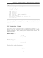
3 Constrained Optimization in One Dimension
3.1 Overview . . . . . . . . . . . . . . . . . . . . . .
3.2 The Graphical User Interface . . . . . . . . . . .
3.3 The Method of Usable Feasible Direction . . . . .
3.4 Sequential Unconstrained Minimization Technique
4 The
4.1
4.2
4.3
Kuhn-Tucker conditions in Two Dimensions
Overview . . . . . . . . . . . . . . . . . . . . .
The Graphical User Interface . . . . . . . . . .
Optimization of the Fiber Reinforced Plate . . .
4.3.1 Load Cases . . . . . . . . . . . . . . . .
4.3.2 Coordinate System Transformation . . .
4.3.3 Constraints . . . . . . . . . . . . . . . .
4.4 Calculating the Lagrangian Multipliers . . . . . .
5 Augmented Lagrangian Procedure
5.1 Overview . . . . . . . . . . . . . . . .
5.2 The Graphical User Interface . . . . .
5.3 The Dual Method . . . . . . . . . . .
5.4 The Augmented Lagrangian Procedure
6 Bibliography
.
.
.
.
.
.
.
.
.
.
.
.
.
.
.
.
.
.
.
.
.
.
.
.
.
.
.
.
.
.
.
.
.
.
.
.
.
.
.
.
.
.
.
.
.
.
.
.
.
.
.
.
.
.
.
.
.
.
.
.
.
.
.
.
.
.
.
.
.
.
.
.
.
.
.
.
.
.
.
.
.
.
.
.
.
.
.
.
.
.
.
.
.
.
.
.
.
.
.
.
.
.
.
.
.
.
.
.
.
.
.
.
.
.
.
.
.
.
.
.
.
.
.
.
.
.
.
.
.
.
.
.
.
.
.
.
.
.
.
.
.
.
.
.
.
.
.
.
.
.
.
.
.
.
.
.
.
.
.
.
.
.
.
.
.
.
.
.
.
.
.
.
.
.
.
.
.
.
.
.
.
.
.
.
.
.
.
.
.
.
.
.
.
.
.
.
.
.
.
.
.
.
.
.
.
.
.
.
.
.
.
.
.
.
.
.
.
.
.
.
.
.
.
.
.
.
.
.
.
.
.
.
.
.
.
.
.
.
.
.
.
.
.
.
.
.
.
.
.
.
.
.
.
.
.
.
.
.
.
.
.
.
.
.
.
.
.
.
.
.
.
.
.
.
.
.
.
.
29
III
List of Figures
2.1
2.2
Applet window - 1D unconstrained. . . . . . . . . . . . . . . . . . . . . . .
One iteration of the iterative minimization procedure. . . . . . . . . . . . .
6
7
3.1
Applet window - 1D constrained . . . . . . . . . . . . . . . . . . . . . . . .
12
4.1
4.2
Applet window - 2D Kuhn-Tucker . . . . . . . . . . . . . . . . . . . . . . .
Fiber reinforced plate - the two load cases . . . . . . . . . . . . . . . . . .
16
18
5.1
5.2
5.3
Applet window - The Augmented Lagrangian Procedure . . . . . . . . . . .
The Dual Method . . . . . . . . . . . . . . . . . . . . . . . . . . . . . . .
The Augmented Lagrangian Procedure . . . . . . . . . . . . . . . . . . . .
22
24
26
1
1 Introduction
The following sections describe a suite of interactive Java applets designed to support the
course Multidisciplinary Design Optimization. The sample problems were chosen to make
them easy to follow.
Thus, unconstrained optimization is illustrated with an objective function in one variable
(Section 2). Then, constraints are added to the same problem (Section 3). For optimization
in multiple dimensions, a 2D case is taken as an example (Section 4). In order to better
understand the concept of the Lagrangian, a method that uses it directly is also implemented
(Section 5).
The illustrative examples enumerated above allow making many important connections to
the material of the lectures [1]. Hopefully, experimenting with the applets can be helpful in
grasping the practical implications of the theory involved.
Concerning the theory in both its mathematical and its algorithmical aspects, the necessary
remarks can be found in the text that follows. Special attention is devoted to those crucial
details that are covered only at an abstract level in the lecture script [1].
Of course, this User’s Guide cannot provide the overall picture of all the relevant topics. For
that, the lecture notes must be consulted. Both detailed and comprehensive treatment of
optimization theory aspects can be found in books [3, 4, 5]. References to those are made
accordingly.
3
2 Unconstrained Optimization in One
Dimension
2.1 Overview
As an introductory example, the problem of unconstrained minimization in 1D is considered.
In the following, the relevant theoretical aspects are outlined and the workings of this particular iteractive implementation are explained. The very next section describes available GUI
controls and how they help to explore the effects of various decisions in the construction of
the minimization procedure. Further, the algorithm of root finding with the method of iterations is explained. In this applet, the minimum is identified as the root of the first derivative
(for the details, see [1, §6.4]). Finally, the three available termination criteria are explicated
with formulas.
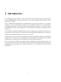
2.2 The Graphical User Interface
The overall view of the applet window is shown in Figure 2.1.
The left part shows a plot of the objective function and on the right there are a number of
panes for controlling the optimization procedure.
Procedure control contains two buttons:
• Minimize runs the procedure with the parameters currently set and displays the intermediate steps in the plot;
• Start over clears the plot to the initial state.
Initial point provides one button and displays a message string. Upon pressing Set start
you will be offered to specify the initial approximation with a mouse click in the
plot.
Objective function offers a choice among the two available objective function.
Gradient calculation allows adjustment of the way in which the derivative of the objective
function is evaluated:
5
CHAPTER 2. UNCONSTRAINED OPTIMIZATION IN ONE DIMENSION
• Analytical: the formula that results from differentiating the objective function by hand
is used.
• Finite differences:
y(x + ∆x) − y(x)
∆x
∆x
) − y(x −
y(x
+
2
central: y 0 (x) =
∆x
y(x)
−
y(x
− ∆x)
backward: y 0 (x) =
∆x
forward: y 0 (x) =
(2.1)
∆x
)
2
(2.2)
(2.3)
Step size accepts a value for the parameter α (explained in section 2.3).
Termination criteria offers a selection of termination criteria (explained in Section 2.4).
Optimization ends as soon as at least one of the criteria that are currently checked on
is fulfilled.
Figure 2.1: Applet window - 1D unconstrained.
6
CHAPTER 2. UNCONSTRAINED OPTIMIZATION IN ONE DIMENSION
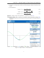
2.3 The Iterative Minimization Procedure
The algorithm described below can be viewed as a (simplified) special case of “the steepest
descent” in 1D, see [1, §6.4]. For numerical optimization, an initial point x0 must be selected
as a rough approximation. A sequence of increasingly better approximations is generated via
the following update rule:
xi+1 = xi − α · ∇y(xi )
The value for xi when i = 0 and the value of α are parameters to the procedure. The derivative ∇y can be evaluated either numerically or analytically, as was mentioned in section 2.2,
Gradient calculation. The update rule is illustrated in Figure 1.2.
Figure 2.2: One iteration of the iterative minimization procedure.
The overall procedure flow may be summarized in pseudo-code as follows (assuming that the
functions y, y_prime, and converged have been suitably defined):
7
CHAPTER 2. UNCONSTRAINED OPTIMIZATION IN ONE DIMENSION
Algorithm
10:
20:
30:
40:
50:
60:
70:
80:
100:
110:
120:
130:
2.1
minimize_iterative(x0, alpha)
i = 0;
xi_1 = x0;
yi_1 = y(xi_1);
do
i = i + 1;
xi = xi_1;
yi = yi_1;
xi_1 = xi - alpha * y_prime(xi);
yi_1 = y(xi_1);
while not converged(xi, yi, xi_1, yi_1, i);
return xi_1;
As can be seen, the call to converged in line 120 accepts both the old and the updated
values of x and y. The next section describes how these values are used to halt the procedure
in due time.
2.4 Termination Criteria
Three different criteria are implemented and can be applied either individually or in combination. In every case, the purpose is to halt the optimization procedure when no further
progress is envisioned, i.e. when xi would stay almost constant in further iterations. The
criteria are as follows.
Relative change in y:
|
yi+1 − yi
|≤ε
yi
Absolute change in x:
|xi+1 − xi | ≤ δ
Predefined limit number of evaluations:
i ≥ imax
8
CHAPTER 2. UNCONSTRAINED OPTIMIZATION IN ONE DIMENSION
The parameters ε, δ, and imax can be set independently for every criterion in the user
interface. When more than one criteria are checked, a change in a parameter sometimes
has no effect on the course of execution. This indicates that the respective criterion does
not cause termination of the algorithm in this particular setting, but rather one of the other
activated criteria does.
Also note that the effect of imax on the number of iterations changes depending whether the
Finite differences or the Analytical mode is selected in the Gradient calculation tab. In the
former case, the counter i in line 60 of Algorithm 1.1 is incremented by two units instead
of one. The difference in the number of evaluations per iteration should be apparent from
formulas 2.1-2.3. Of course, with finite differences function evaluations are counted, not
evaluations of the analytical derivative.
9
3 Constrained Optimization in One
Dimension
3.1 Overview
The following sections describe the applet that illustrates two approaches to constrained
optimization. The sample problem is identical to the one considered previously (see Section
2), just the constraints are added. Therefore, the user interface contains some additional
controls, which are described in the next section.
Sections 3.3 and 3.4 provide references concerning two methods based on the iterative procedure (Section2.3).
• The method of usable feasible direction is quite a straightforward extension, just one
more termination criterion is added. An outline of this principle can be found in [1,
§6.6].
• Sequential unconstrained minimization technique (SUMT) constructs an auxiliary function that automatically takes the constraints into account (for details please consult
[1, §6.2]).
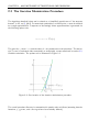
3.2 The Graphical User Interface
The applet window is shown in Figure 3.1 with the additional control pane expanded. The
rest of the panes are the same as in LLBoApplet1, please refer to Section 2.2 for details.
The Methods pane contains two radio buttons and also the means to fine-tune the factor r:
• Usable feasible direction activates the simple way of constraint handling, it has no
parameters (see Section 3.3).
• SUMT activates Sequential Unconstrained Minimization Technique, which depends on
parameter r (see Section 3.4).
• The text field labeled [ r = ] accepts the value for r. The new value is applied upon
the next minimization run (invoked via the Minimize button in the Procedure control
pane).
11
CHAPTER 3. CONSTRAINED OPTIMIZATION IN ONE DIMENSION
• The buttons labeled [ / 10 ] and [ * 10 ] serve to automatically scale r by an order
of magnitude with every click. Besides, they simultaneously produce a convenient side
effect: the currently achieved minimum is set as the initial approximation x0 for the
next run (see Section 2.3).
Figure 3.1: Applet window - 1D constrained
12
CHAPTER 3. CONSTRAINED OPTIMIZATION IN ONE DIMENSION
3.3 The Method of Usable Feasible Direction
For the 1D setting the method under consideration is trivial. Another termination criterion
that is added internally to the algorithm is all that changes compared to the basic steepest
descent (see Section 2.3). This additional criterion is simply, “as soon as xi+1 lies outside
the feasibility region, return xi as an optimum.” One example of how the same principle is
applied in a more sophisticated context is Sequential Quadratic Programming (SQP), see [1,
§6.6].
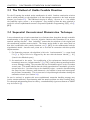
3.4 Sequential Unconstrained Minimization Technique
A more advanced way to hanle constraints is to eliminate them altogether through a suitable
transformation of the problem: from the objective function with constraints to an unconstrained auxiliary function1 . Here “suitability” means that the solutions of the original and
the transformed problems must coincide. The lecture script dwells in quite some detail on
how this is achievable with penalty functions, see [1, §6.2] for the mathematical and the
algorithmical details. Just two more points are to be made in connection with this specific
implementation:
1. For illustrative purposes, the algorithm is left to be “semi-automatic”, i.e. steps 4 and
5 in [1, p. 76] are left to be triggered by the user with the button labeled [ / 10 ]
(found in the Methods pane).
2. As mentioned in the script, “the conditioning of the replacement function becomes
increasingly worse as r becomes smaller” ([1, p. 76]). Indeed, this may manifest itself as
an error message reading ’The procedure led into an infeasible region’ in the Procedure
control pane. This would indicate that the initial approximation is unsuitable, given the
current value for α. In order to keep to the feasibility region, α must be decreased using
the Step size pane. However, with decreased α the number of steps until convergence
may become unreasonable. This in turn can be helped through somewhat relaxing the
temination criteria (see Section 2.4).
As can be noticed, in practice this more sophisticated constraint handling strategy may
involve certain subtleties. Experimenting with the sample problem can help revealing them.
For thorough understanding based on theory, a mathematically rigorous treatment of SUMT
may be found in [3].
1
Also called “replacement function” in [1].
13
4 The Kuhn-Tucker conditions in Two
Dimensions
4.1 Overview
The applet described below illustrates some fundamental aspects of optimization in multiple
dimensions. To keep the example comprehensible, a problem in just two dimensions is
considered.
The very next section describes the user interface, which displays the 2D space of design
variables, the objective function, the constraints, and some supplementary visual clues.
Further, the design problem to be considered is introduced (Section 4.3). Evaluation and
analysis of the Kuhn-Tucker conditions (see [1, §3.6]), which form the essence of this applet,
is discussed last (Section 4.4).
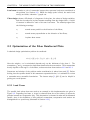
4.2 The Graphical User Interface
The overall view of the applet window is shown in Figure 4.1. A 2D plot on the left represents the design space in variables α and d (see Section 4.3 for a reference to the problem
statement). A click in the plot selects the point to analyse. On the right there are three
panes that display characteristics of the currently selected design space point.
Lagrangian multipliers displays the following values once they are calculated:
1
λ1,2
The values of the Lagrangian multipliers selected through application
of the least squares method , see Section 4.4 for details.
L
The value of the selected Lagrangian at the current point.
∇x1,2 L
The gradient of the selected Lagrangian1 at the current point (allows
judging whether the point can be an optimum).
Note that the multipliers λ1,2 are calculated to be the best in the least squares sense. The values thus
obtained differ over the neighbourhood of a given point in the design space. It should be noted that both
the value and the gradient of the Lagrangian depend on these multipliers. Essentially, a different function
L is considered in every design point. Therefore, the habitual relation between function derivatives and
how the function itself varies cannot be expected to hold in this particular case.
15
CHAPTER 4. THE KUHN-TUCKER CONDITIONS IN TWO DIMENSIONS
g1,2
The values of the constraint functions (allow judging whether the
point lies within the feasibility region).
x1,2
The values of the design variables (x1 and x2 correspond to α and
d, respectively).
The Calculate multipliers button makes the current point fixed and triggers
caluclation of the values enumerated above. The Reset button produces the
reverse effect, the values disappear and the selected point again traces the mouse
pointer freely, thus updating the Plate design pane.
Figure 4.1: Applet window - 2D Kuhn-Tucker
16
CHAPTER 4. THE KUHN-TUCKER CONDITIONS IN TWO DIMENSIONS
Load cases contains a pair of mnemonic images that represent load cases considered in
the problem (see Section 4.3). When the design point is fixed, the active load
case(s) are black; otherwise - grayed out.
Plate design shows a 3D sketch of a fragment of the plate, the values of design variables,
and also six values for in-plane stresses resulting from the design choice. A triple
of stresses is defined for each of the two load cases. The subscript signs have
the following meanings:
σ||
normal stress parallel to the direction of the fibers;
σ⊥
normal stress perpendicular to the direction of the fibers;
σ]
in-plane shear stress.
4.3 Optimization of the Fiber Reinforced Plate
A classical design optimization problem is considered:
min {w(d) | g1 (α, d) ≤ 0, g2 (α, d) ≤ 0}
Here the weight w to be minimized depends only on the thickness of the plate d. The
constraints g1 and g2 correspond to load cases described in the next section. These constraints
heavily depend on the angle α of the fibers, as becomes clear from sections 4.3.2 and 4.3.3.
Statement and solution of the problem under consideration is taken from work [2]. Before
delving into the specific details of this statement expounded below, it is advisable to review
a somewhat more accessible formulation. The lecture script [1, §2.1.3] can be helpful in
gaining an overall picture.
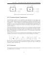
4.3.1 Load Cases
The specific load values that were used as an example in this implementation are given in
Figure 4.2. Regarding load case g2 it can be observed that due to the choice of values the
principal stresses are compressive only. This observation is relevant for what will be discussed
further, since in the definition of this problem’s constraints, compression and tension are
distinguished in a special way (discussed in Section 4.3.3).
17
CHAPTER 4. THE KUHN-TUCKER CONDITIONS IN TWO DIMENSIONS
Figure 4.2: Fiber reinforced plate - the two load cases
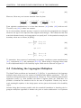
4.3.2 Coordinate System Transformation
The loads shown in Figure 4.2 are expressed as forces distributed over the length of the
edges of a plate element. In other words, integration of stresses over plate thickness has
been performed. The constraints that will be discussed in a moment are formulated in terms
of stresses σ|| , σ⊥ , and σ] . Therefore, the values of distributed forces are to be divided by
thickness d in order to obtain stresses. Moreover, the stresses must be transformed to the
coordinate system that is aligned to the direction of the fibers (in other words, the system is
rotated by angle α).
The needed transformation involves two rotations. First, it is necessary to calculate horizontal
and vertical components of stresses at the edges of a rotated element of the plate. Second,
these components must be expressed relative to the rotated axes of the new coordinate
system. This explains why the transformation matrix in (4.1) has products of trigonometric
functions as its elements.
Uniting all that was said so far, the following formula allows arriving from distributed forces
(defined by the load cases) to fiber-aligned stresses (used for defining the constraints):
cos2 α
sin2 α
2 · sin α · cos α
F11
σ||
1 
 


2
2
sin α
cos α
−2 · sin α · cos α  ×  F22 

 σ⊥  = · 
d
− sin α · cos α sin α · cos α cos2 α − sin2 α
F12
σ]






(4.1)
As can be seen, all derived quantities are obtained analytically. However, the expressions
became quite involved already. More complications are added at the stage of defining the
constraints, which is discussed next.
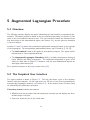
4.3.3 Constraints
The requirement that the fibers must not suffer damage is formulated in terms of the boundary allowable stress σ|| B as follows:
18
CHAPTER 4. THE KUHN-TUCKER CONDITIONS IN TWO DIMENSIONS
σ|| (α, d)
σ|| B
!2
−160
(4.2)
Moreover, fibers may not become detached from the plate:
σ|| (α, d)
σ|| B
!2
σ⊥ (α, d)
+
σ⊥ B
!2
σ] (α, d)
+
σ] B
!2
−160
(4.3)
From algebraic considerations it is clear that whenever (4.3) holds, (4.2) holds as well.
Therefore, only (4.3) is taken into account.
As for the boundary allowable stresses, it must be noted that their magnitudes are changed
whenever the sign of the respective fiber-aligned stress changes. This reflects the fact that
materials withstand tension and compression not equally well. In this particular example, the
boundary values are as follows (in [MPa]):
σ|| B =

200
75
for σ|| > 0
for σ|| < 0
σ] B = 6.1

4.8
for σ⊥ > 0
σ⊥ B = 
15.5 for σ⊥ < 0
(4.4)
(4.5)
(4.6)
To summarize, three sources of nonlinearity are present: coordinate system transformation
(4.1), requirement (4.3), and parameters (4.4, 4.6). When acting in sequence these result
in the complicated shape of the feasibility region, which can be observed in Figure 4.1.
4.4 Calculating the Lagrangian Multipliers
The Kuhn-Tucker conditions are introduced in [1, §3.6] as “a generalization of the Lagrange
multiplier theory that is true for extrema of functions with equality restrictions.” The construction of this generalization is explicated in [4, Chapter 5]. There, additional mathematical
apparatus is used, e.g. slack variables, the notion of regular points, etc. With that, it is
possible to formulate the conditions also for the case of inequalities. Besides, they can be
made meaningful anywhere in the design space and not just at the bounds of the feasibility
region.
Another thing that becomes possible with the extended formulation is obtaining the Lagrangian multipliers regardless of whether the point x under consideration is an optimum
19
CHAPTER 4. THE KUHN-TUCKER CONDITIONS IN TWO DIMENSIONS
or not. The vector λ is calculated under an a priory assumption that the primary condition
holds:
X ∂gj
∂L
∂f
=
−
=0
λj
∂xi
∂xi
∂xi
j
Or, in matrix form:
∇f − N λ = 0
Here ∇f is the gradient of the objective function at point x, and N is defined by nij =
(4.7)
∂gj
.
∂xi
The following formula from [4] approximates λ as a solution to (4.7) in the least squares
sense:
λ = NT N
−1
N T ∇f
(4.8)
Once the multipliers are calculated, the gradient of the Lagrangian ∇L at point x can be
obtained. One of the following things then happens:
1. ∇L is zero. This indicates that the formula (4.8) produced an exact solution to
equation (4.7), and x may be an optimum. The rest of the conditions must be
checked.
2. ∇L is nonzero. This means that the initial assumption was wrong and x cannot be
an optimum.
20
5 Augmented Lagrangian Procedure
5.1 Overview
The following sections describe the applet illustrating the dual method of constrained optimization. The sample problem is similar to the one considered previously (see Section 3), but
there is only one constraint instead of two. The user interface controls are identical to the
first three panes in the unconstrained applet (see Section 2.2), and the plots are described
in the next section.
Sections 5.3 and 5.4 outline two constrained optimization strategies based on the concept
of the Lagrangian. The corresponding mathematical theory can be found in [5, Ch 17].
• The dual method is used in this guide for introductory purposes. The applet itself is
implemented in a more sophisticated way.
• The Augmented Lagrangian Procedure (ALP) is a further development aiming at
better stability and faster convergence. The implemented algorithm is given in full
detail as a flow chart in Figure 5.3. However, only the most fundamental aspects are
thoroughly commented upon.
For a detailed treatment of the topic, please refer to [5].
5.2 The Graphical User Interface
The applet window is shown in Figure 5.1. The left part shows a plot of the objective
function and the constraint. On the right there is a 2D plot of level lines representing the
corresponding Lagrangian function (see Section 5.3). At the bottom there are three panes
for controlling the optimization procedure:
Procedure control contains two buttons:
• Minimize runs the procedure with the parameters currently set and displays the intermediate steps in the plot;
• Start over clears the plot to the initial state.
21
CHAPTER 5. AUGMENTED LAGRANGIAN PROCEDURE
Initial point provides one button and displays a message string. Upon pressing Set start
you will be offered to specify the initial approximation with a mouse click in
either of the two plots.
Objective function offers a choice among the two available objective function.
Figure 5.1: Applet window - The Augmented Lagrangian Procedure
5.3 The Dual Method
Along the lines of a more general case [5, §17.1], let us consider the Lagrangian function
that corresponds to the 1D constrained optimization problem with one equality constraint:
22
CHAPTER 5. AUGMENTED LAGRANGIAN PROCEDURE
L(x, λ) = f (x) + λg(x),
where f (x) is the objective function, g(x) - the constraint, and λ- the Lagrangian multiplier.
Now we can define the dual function D(λ),which is the minimum of L(x, λ) along x when
λ is fixed to a certain value as the independent variable:
D(λ) = minx L(x, λ)
The optimum of the constrained problem is defined as the saddle point of the Lagrangian.
Using the definitions introduced above, at the optimum it holds:
maxλ D(λ) = minx L(x, λ)
Conventional descent methods are not applicable for finding saddle points. Still, an iterative
procedure called the dual method can be constructed as a sequence of repeated minimizations
while λ is adjusted:
1. Given L(x, λ) = f (x) + λg(x), assume some initial λ = λk , k = 0.
2. Obtain the intermediate optimal solution x∗ (λ) = minx L(x, λ).
3. Modify λ = λk+1 .
4. Repeat steps 2 and 3 until convergence.
An open question here is how to modify λ. One possibility is to change it by the value of
the constraint g at current point x, multiplied by certain factor 1/µ:
λk+1 = λk +
g(x∗ (λk ))
µ
The reasoning behind this formula goes like this, “If constraint g is still violated at the
saddle point, this means that the lagrangian multiplier λ is not large enogh”. In case the
iterative process does not converge, this indicates that factor µ should be decreased. The
resulting algorithm is presented as a flowchart in Figure 5.2. To make the update rule for
λ mathematically sound, we need to augment the Lagrangian function with an extra term,
which is discussed in the next section.
23
CHAPTER 5. AUGMENTED LAGRANGIAN PROCEDURE
λk−1 = λk = 0
x = x0
f k = L(x, λk )
L0x k = L0x (x, λk )
f k = f k+1
L0x k = L0x k+1
α = α0
α = α/2
f k+1 = L(x − α · L0x k , λ)
L0x k+1 = L0x (x − α · L0x k , λ)
T
F
f
k+1
k
≤ (f − σ · α ·
L0x k )
x = x − α · L0x k
T
|L0x k+1 | ≤ xT ol
F
λk−1 = λk
λk = λk + g(x)/µg
F
T
k
|λ − λ
k−1
| ≤ λT ol
DONE
Figure 5.2: The Dual Method
24
CHAPTER 5. AUGMENTED LAGRANGIAN PROCEDURE
5.4 The Augmented Lagrangian Procedure
The ALP (see [5, §17.5]) is similar to the penalty method in that a penalty term is added
(see Section 3.4). But to avoid an ill-conditioned problem in the end, it is added not to the
objective function itself but rather to the Lagrangian. If we take g to be again an equality
for a start, the Lagrangian is augmented as follows:
LA (x, λ; µ) = L(x, λ) +
1 2
1 2
g (x) = f (x) + λg(x) +
g (x)
2µ
2µ
From the Kuhn-Tucker condition by certain transformations it follows that near a critical
point this holds:
λ+
g(x)
≈ λ∗
µ
The above suggests an update rule for converging to the correct value for lambda. From
this, the following algorithmic framework results:
1. Start with initial approximation x0 , λ0 , and a chosen factor µ0 > 0. Request final
tolerance tol. For k = 0, 1, 2 . . .
2. Starting from xk , minimize LA (x, λk ; µ) until
k OLA (x, λk ; µ) k< τk
The result of minimization is x∗k .
3. If τk < tol - we are done!
Else
λk+1 = λk + µ1 g(x∗k )
xk+1 = x∗k
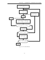
The flowchart for the resulting algorithm is shown in Figure 5.3.
25
λk−1 = λk = 0
x = x0
xT ol = xT ol0
s1 = max(g(x), 0)
k=1
α = α0
k =k+1
T
F
α = α0
k == 2
f k = LA (x, sk , λk )
L0x k = LA 0x (x, sk , λk )
F
T
|L0x k | ≤ xT ol
L0x k+1 = |L0x k |
sk+1 = max(g(x − α · L0x k ), 0)
f k+1 = LA (x − α · L0x k , λk )
L0x k+1 = LA 0x (x − α · L0x k , λk )
α = α/2
F
f
k+1
T
L0x k )
k
≤ (f − σ · α ·
x = x − α · L0x k
sk = sk+1
T
F
L0x k+1 ≤ xT ol
sk = max(g(x), 0)
f k = f k+1
L0x k = L0x k+1
T
F
k == 1
k−1
λ
=λ
k)
k
λ = λ + (g(x)−s
µ
k
T
T
xT ol = xT ol/3
|λk − λk−1 | ≤ λT ol &&
|L0x k+1 | ≤ xT ol
|L0x k+1 | ≤ xT ol &&
xT ol > xT olM in
T
DONE
F
F
|λk − λk−1 | ≤ λT ol &&
|L0x k+1 | ≤ xT ol
F
CHAPTER 5. AUGMENTED LAGRANGIAN PROCEDURE
It can be seen that the flowchart contains a number of algorithmic features in addition to
those outlined in the framework. They were added as improvements and are sometimes
heuristic in nature. The purpose and main ideas of these enhancements are briefly outlined
below:
1. Slack variable s is used to account for the fact that g is in fact inequality constraint.
An expression (g(x) − s) is used in place of g(x), and s is kept equal to max(0, g(x)).
2. Adjustment of α is needed to ensure stability of the search along x. Armijo condition
(see [5, §3.1]) is used to determine whether α is small enough to produce sufficient
decrease in the objective function value, and σ is a parameter to that condition.
3. Multi-step optimization along x for k = 1 allows to reach good approximation
of the intermediate optimum during the first run along x, regardless of the initial x0 .
This allows making just one optimization step along x per every adjustment of λ.
4. Adjustment of xT ol can result in this parameter changing by as much as three orders
of magnitude during an optimization run. It improves efficiency to opt for less precise
but faster solutions while the final optimum is far away. As the method converges, the
precision is gradually increased.
27
6 Bibliography
[1] Baier, Horst; Huber, Martin; Petersson, Ögmundur; and Wehrle, Erich. Multidisciplinary
Design Optimization, Lecture Notes.
[2] Baier, Horst; Mathematische Programmierung zur Optimierung von Tragwerken insbesondere bei mehrfachen Zielen, Dissertation. Darmstadt, 1978.
[3] Fiacco, Anthony V. and McCormick, Garth P. Nonlinear programming: sequential unconstrained minimization techniques. Philadelphia: SIAM, 1990.
[4] Haftka, Raphael T. abd Gürdal, Zafer. Elements of structural optimization. Dordrecht:
Kluwer Academic Publishers, 1992.
[5] Nocedal, Jorge and Wright, Stephen. Numerical Optimization. New York: SpringerVerlag, 2000.
29