Download User guide

User guide
To develop matrices for ESTScan
Ludivine Rielle
Directed by Prof. Victor Jongeneel
Supervised by Christian Iseli
Janvier 2007
1
Contents
1.
Introduction............................................................................................................................4
2.
Required configuration...........................................................................................................5
3.
Content of the ESTScan package............................................................................................6
4.
Configuration file ...................................................................................................................7
4.1.
Description of the configuration file ...............................................................................7
4.2.
Creation of the configuration file ....................................................................................8
4.2.1.
Opening a configuration file....................................................................................8
4.2.2.
Changing the species’ name ....................................................................................8
4.2.3.
The variable $hightaxo............................................................................................9
4.2.4.
Location of the downloaded files ............................................................................9
4.2.5.
Location of new files ............................................................................................10
4.2.6.
Number of isochores .............................................................................................10
4.2.7.
Number of tuplesize..............................................................................................11
4.2.8.
Number of minmask .............................................................................................11
5.
Sequences to download ........................................................................................................12
6.
Isochores..............................................................................................................................14
7.
Obtaining the matrices..........................................................................................................17
8.
Evaluation of the matrices ....................................................................................................19
9.
Input and output of scripts ....................................................................................................20
9.1.
Input and output of extract_mRNA...............................................................................20
9.2.
Input and output of prepare_data...................................................................................20
9.3.
Input and output of build_model ...................................................................................21
9.4.
Input and output of extract_UG_EST............................................................................21
9.5.
Input and output of evaluate_model ..............................................................................22
2
10.
Results .............................................................................................................................23
10.1.
Description of the results ..........................................................................................23
10.2.
How to use the results ...............................................................................................27
10.2.1.
The report’s files...................................................................................................27
10.2.2.
The files ending with “gplot” ................................................................................28
10.2.3.
The file ending with “.R” ......................................................................................28
11.
Conclusion .......................................................................................................................29
12.
Appendix..........................................................................................................................30
12.1.
RefSeq format...........................................................................................................30
12.2.
EMBL format ...........................................................................................................31
12.3.
UniGene Format .......................................................................................................31
12.4.
Example of ug.data file: ............................................................................................33
12.5.
Example of cluster.lst file .........................................................................................34
12.6.
Example of matches.lst file .......................................................................................34
13.
References........................................................................................................................35
14.
Web site references ..........................................................................................................36
3
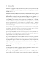
1. Introduction
ESTScan is a bioinformatic tool that permits the analysis of ESTs (expressed sequence tags). The
program scans the ESTs, detects their coding part even if they are of low quality, and corrects the
frameshift errors [6, 8, 9].
ESTScan takes advantages of the known associated bias in hexanucleotide composition, imposed
by species dependent codon usage biases and amino acid composition inhomogeneities. This bias,
which is used as a component in many gene prediction algorithms [2,3], was formalized as an
inhomogeneous 3-periodic fifth-order Hidden Markov Model (HMM) in the ESTScan program
[5]. This HMM has been extended to allow for various types of sequencing errors: (1) frameshift
errors that would destroy the periodicity of the Markov chain; (2) sequencing errors that would
introduce erroneous stop codons; (3) the presence of a considerable number of ambiguous
nucleotides. It has also been normalized to correct biases introduced by the length of the sequence
and its G+C isochore group.
In order to function correctly, the program needs some scores matrices which are normally specific
for each species. These matrices reflect the codon preferences in the studied organism and can be
obtained by using three scripts: extract_mrna, prepare_data and build_model.
The first script, extract_mrna extracts the data from files previously downloaded from FTP sites.
The extraction is done by taking the sequences, contained in files, that correspond to a species or to
a higher taxonomic level according to what has been chosen by the user.
The second script, prepare_data, classifies the mRNAs extracted previously. First, it separates the
mRNAs in two groups: training and test data, if the user chooses to separate them. If he does not,
the same data will appear in both files. Second, the training data is divided according to the
mRNAs’ GC-content. Third, the redundancy is masked. Fourth, the coding and non-coding parts of
mRNAs are classified in two different files.
Finally, the third program called build_model creates the matrices using the data prepared by the
previous scripts.
Following this, it could be useful to evaluate the efficiency of the matrices. This step is done by
using two different scripts: extract_UG_EST and evaluate_model.
The first script, extract_UG_EST, uses UniGene clusters produced by the NCBI [12, 15]. A
cluster is composed of ESTs that match a genomic sequence with an annotation making reference
4
to RefSeq or EMBL mRNA sequence. This script searches for the clusters that correspond to the
mRNAs of the test file. All clustered ESTs are aligned with their respective mRNA with
megablast. The alignment enables the annotation of the ESTs and their classification into two main
groups: coding or non-coding sequences.
The second program called evaluate_model evaluates the matrices. It launches ESTScan on data
that have been obtained previously in order to predict the coding parts.It then calculates the false
negative rate (sensitivity): the percentage of coding sequences classified as non-coding, the false
positive rate (specificity): the percentage of non-coding sequences classified as coding and the
detection accuracy of the start and stop sites.
The use of the different programs is not difficult. Nevertheless, this user guide will assist people
using ESTScan during the first stages: the writing of the configuration file, which contains
information required for the programs and the execution thereof.
2. Required configuration
The use of ESTScan requires:
-The use of a computer that has a C compiler and manage to use the Perl language.
-The download of the programs from http://sourceforge.net/projects/estscan/:
- Download all the files from the BTLib package
- Download all the files from the ESTScan package, version 3.0.
-The
download
of
megaBLAST
[13]
distributed
from
the
NCBI
FTP
site:
ftp://ftp.ncbi.nlm.nih.gov/blast/ under the /blast/executables/ directory. Some information is
available on the blast/documents/ directory of this FTP site.
-The download of R and gnuplot; in most cases, they are in the Unix distribution.
-The download of files containing sequences from the RefSeq, EMBL and UniGene FTP sites.
One should bear in mind that the creation of the matrices implies the use of mRNAs that must be
annotated and must contain the entire coding region. Without these two conditions being met, it
is impossible to create reliable matrices.
Note: the explanations in this user guide consider that the user has chosen a UNIX environment,
for example Fedora [19].
5
3. Content of the ESTScan package
Some information, reports and links are available at http://estscan.sourceforge.net/.
The programs that must be downloaded are available from http://sourceforge.net/projects/estscan/.
There are fives groups of files:
- The BTLib files that are necessary for the partitioning of the EMBL or RefSeq files.
- The ESTscan package that contains all the programs required to run the program on
sequences (version 3.0).
- The ESTscan1 package
- The ESTscan2 package
- Some matrices with their evaluation.
All the scripts needed to create and evaluate the matrices are available in files in the ESTScan
package version 3.0:
- estscan-devel-3.0-0.i386.rpm
- estscan-devel-3.0-0.ia64.rpm
- estscan-devel-3.0-0.x86_64.rpm
6
4. Configuration file
The use of ESTScan implies the creation of matrices that reflect the codon preferences of the
species of interest. All the scripts used to create or evaluate these matrices need a configuration
file that contains the main piece of information.
4.1. Description of the configuration file
The configuration file must be in Perl syntax; it looks as follows.
################################################################################
#
# Parameters for the mouse
# (use PERL syntax!)
#
$organism
= "Mus musculus";
$hightaxo
= "Rodentia";
$dbfiles
="/db/refseq/release/mus*.gbff
/db/refseq/new/mus*.gbff
/db/embl/86/mus*.dat
/db/embl/new/mus*.dat";
$ugdata
= "/db/unigene/Mm.data";
$estdata
= "/db/dbest/est_mus-??.seq";
$datadir
= "/ESTScan/Results/Mm";
$nb_isochores
= 2;
$tuplesize
= 6;
$minmask
= 30;
#
# End of File
#
################################################################################
7
The first variable $organism contains in quotation marks the name of the species you are
interested in. This variable is used to select entries in files containing information for various
species.
$hightaxo is a variable that can be used to consider sequences from a group of species instead of
only involving those from one species. It contains a taxonomic level that has been chosen by the
user (see section 5).
$dbfiles specifies the local files, in EMBL or RefSeq format, from which full-length mRNA
sequences are extracted.
$ugdata specifies the files containing the UniGene clusters.
$estdata specifies the files containing ESTs.
$datadir is the base directory where all the files are located and the temporary results are stored.
$nb_isochores or @isochore_borders allows the separation of the training data according to their
GC content (see section 6).
$tuplesize indicates the order of the Hidden Markov Model; its default value is 6.
Finally $minmask is a parameter used during masking redundancy. It indicates the threshold
length above which redundant pieces of sequences will be masked. Its default value is 30.
4.2. Creation of the configuration file
4.2.1.
Opening a configuration file
For the generation of matrices for a specific species one needs to follow a series of steps in order to
create the configuration file which allows the use of the scripts.
The
first
step
is
to
copy
a
configuration
file
(“.conf”
ending)
available
from
http://estscan.sourceforge.net/.
Save this file with a name that reminds you of the content of the file, for example: hs.conf for the
configuration file for human sequences.
4.2.2.
Changing the species’ name
One configuration file per species has to be written for it to be used during the execution of the
scripts. Thus it is necessary to replace the name of the species by the name of the species you are
interested in.
8
Changing the name on the first line
You have to change the name written in the first line after “parameter for” in order to inform users
that this file corresponds to a specific species.
Changing the name following the variable $organism
You also have to change the name of the species that is stored in the variable $organism.
Pay attention to the spelling and the capital letters, because they are essential for the program to
find the entries corresponding to the species of interest (e.g.: Homo sapiens). In case of doubt,
check for species names on the NCBI website [14].
4.2.3.
The variable $hightaxo
If there is not enough data available in databases for the species of interest, you need to add the
variable $hightaxo below $organism. Choose the taxonomic level from which the data will be
extracted on the taxonomic part of the NCBI’s website [21] and write this level after $hightaxo. Do
not forget to use quotation marks and to put a semicolon at the end of the line.
If you want to use the sequences of one organism only, do not add the $hightaxo variable or leave
a space between the quotation marks. Remember that $hightaxo has priority over $organism, thus
the files will be processed according to this $hightaxo variable and not according to $organism
(see section 5).
4.2.4.
Location of the downloaded files
The mRNA or ESTs sequences can be provided as several files. The name of these files must be
contained in the configuration file.
There are two methods for indicating the files to the program: -globbing
-listing of all files
In order to refer to several sequences with similar file names, use an asterisk (*) to replace a part of
the files name or use a question mark (?) to replace one character only. Remember that the Unix
separation of directories is a slash (/).
RefSeq sequences
After $dbfiles you need to indicate the file names in quotation marks.
For example: $dbfiles = “/db/refseq/release/mus*.gbff”;
The asterisk replaces the number written after the abbreviation of the species (e.g. 01, 02, 03,... of
mus01.gbff, mus02.gbff, mus03.gbff)
9
EMBL sequences
You have to indicate the location as previously described just after the information for the RefSeq
sequences. Again, use the asterisk to indicate that you require multiple sequences.
For example: $dbfiles = “/db/refseq/release/mus*.gbff /db/embl/new/mus*.dat”;
UniGene sequences
Indicate the location of the requisite file after $ugdata in the same way as for the RefSeq and
EMBL sequences files. This time you do not need to use the asterisk because there is only one file.
For example: $ugdata = “/db/unigene/Mm.data”;
DbEST sequences
The variable $estdata specifies the location of the ESTs that will be analyzed later. This variable is
not necessary at the moment, however, we can specify the location of the files after $estdata.
For example: $estdata = “db/dbest/est_mus-??.seq”;
4.2.5.
Location of new files
Add in quotation marks after $datadir where the results of the build_model program should be
stored.
For example: $datadir
= “ /home/user/ESTScan/Results/Mm”;
To create some new directories use either the windows-like graphical interface or the terminal. If
you use the shell, enter the directories with the order cd followed by the name of the directories
and then use the order mkdir to create directories.
4.2.6.
Number of isochores
The coding potential of sequences can change according to the GC percentage (reviewed in [1]). In
order to obtain better matrices, one should separate the data according to their GC content.
The user can specify the desired number of isochores. The program will then calculate the
delimitation of the different isochores in order to have the same number of sequences in each
group.
It is also possible to specify the delimitation of the isochores. In this case, the program will apply
the parameter specified by the user and the number of sequences in each group may vary a lot.
10
Number of isochores
If you have no specific idea of the GC percentage distribution, it is advisable to simply choose a
number of isochores. The value can be chosen arbitrarily and then written beside $nb_isochores
(see section 6).
Delimitation of the isochores
In the case that you have a publication that explains the content of the genome of interest, specify
the delimitation of the isochores. Replace $nb_isochores with @isochore_borders and indicate
the isochores’ borders after it (e.g. @isochore_borders = (0.0, 43.0, 47.0, 51.0, 100.0)).
4.2.7.
Number of tuplesize
The tuple size indicates the number of nucleotides used in the Hidden Markov Model. Its default
value is 6.
The user has to indicate the number of tuples after the variable $tuplesize.
4.2.8.
Number of minmask
In order to avoid biases in the training data, redundant pieces of sequences longer than a given
threshold should be masked. The threshold can be set using the variable $minmask.
Its default value is 30. Write this number after $minmask.
11
5. Sequences to download
The amount of data available on FTP sites like EMBL or RefSeq can vary a lot depending on the
species. For some organisms the amount of data will be sufficient to create reliable matrices.
For other organisms, not enough data is available. You may download files from other species
which are phylogenetically closely related. In this case, the user has to choose a higher taxonomic
level from which all the sequences will be extracted. The choice of this level can be done with the
help of the taxonomic browser of the NCBI website [21]. This website provides the lineage of
species and also the classification of some model organisms that can help understand the
phylogeny.
For example:
If you want to analyze some ESTs of the beetle (Tribolium castaneum) :
You can find its abbreviated taxonomy (which is the same as that used in EMBL and RefSeq) in
the taxonomy part of the website of the NCBI:
Eukaryota; Metazoa; Arthropoda; Hexapoda; Insecta; Pterygota; Neoptera; Endopterygota;
Coleoptera; Polyphaga; Cuccjiformia; Tenebrionidae; Tribolium
If you have a look at the classification of model organisms, you will discover that the closest
organism commonly used in molecular research projects is Drosophila melanogaster. In this case,
one solution is to involve all the sequences of the Insecta class.
When we extract the data of Tribolium castaneum in RefSeq and Embl database (data available on
15th december 2006) we obtain only 239 sequences, whereas the extraction of the data for the
insecta class provides 50'361 sequences. Thus we may suppose that the matrix obtained with 239
sequences of the beetle would not be reliable as there is not enough data to permit a significant
training of the program. Using the data for all insects allows one to obtain matrices that are
useable, and thus a better analysis of the ESTs using ESTScan.
To discover how many sequences are required to obtain reliable matrices, we build matrices with
different numbers of sequences. We see that at least 2000 sequences are required.
12
In practice, the user has to add the variable $hightaxo in the configuration file to indicate the
taxonomic level. The program will process all the sequences of organisms in this taxonomic level
and use them to build the matrices (see section 4.2.3).
For example: $hightaxo = “Insecta”;
Moreover, there is sometimes one file per species in the databases, but commonly there are the
sequences of many species in one file. Thus the user has to download the file that contains the
sequences of the species of interest or taxonomic group, and then the program will use the
sequences of interest only (species or the taxonomic group). The sequences of other species or
groups will be excluded from the analysis.
13
6. Isochores
At the beginning of the 1970s, centrifugations in analytical CsCl density gradients of warmblooded vertebrate DNAs showed a compositional heterogeneity, which is not the case for coldblooded vertebrates.
The analysis of the DNA by centrifugation in Cs2SO4 density gradients in the presence of
sequence-specific DNA ligands (e.g. Ag+) then allowed the identification of families of DNA
fragments. These families are characterized by different GC levels. Long DNA stretches (more
than 300 kb) that contain local similarities in GC content are called isochores.
If this type of analysis is applied to human DNA preparations in the 30-100 Kilobase (Kb) size
range, we can observe 5 families, two with GC-poor major components (L1, L2) representing
about two thirds of the genome and three GC-rich components (H1, H2, H3). Furthermore, the
gene distribution is not uniform in the genome. Most of the genes are localized in component H3,
which is the most heterogeneous component and represents 3-5 % of the genome (reviewed in [1]).
Nowadays, if the genomic sequence is available, it is possible to use a computer to analyse the GC
content and to discover the presence of isochores. The bioinformatics approach has mostly
replaced the experimental studies using the CsCl density gradient.
The use of ESTScan implies the choice of some parameters, like the number of tuple or the
number of isochores. Defining the isochores number can be quite difficult. We can analyse the GC
content using a computer or refer to some articles that report the border for the different isochores
present in the species and explain their significance [4], but this information does not exist for
every species.
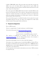
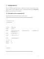
In order to show the effect of the number of isochores on the false positive and false negative rates
of ESTScan, we performed the analysis on mRNAs and ESTs data, using different matrices
created with a variable number of isochores. We can see that the number of isochores does not
seem to be of major importance (Figure 1). There are no significant differences between the
groups.
14
Evaluation of the matrix on ESTs
25,00%
Hs
20,00%
Hs_1is
15,00%
Hs_2is
Hs_4is
10,00%
Hs_47
5,00%
Hs_6is
Hs_8is
0,00%
false positive
rate (nt)
false positive
rate (seq)
false negative
rate (nt)
false negative
rate (seq)
Figure 1: Representation of the false positive and negative rates on the nucleotide and sequence
levels, using matrices created with different number of isochores. The Hs training data was split
into four isochores, with the borders: 0.0, 43.0, 47.0, 51.0, 100.0. The data of Hs_47 was divided
into two parts, choosing 47 as a boundary. The other groups are composed of a variable number of
isochores indicated after Hs. The boundaries are chosen by the computer in order to have the same
number of data in each group.
start predicted at distance
10000
9000
8000
7000
6000
5000
4000
3000
2000
1000
0
Hs
Hs_1is
Hs_2is
Hs_4is
Hs_47
Hs_6is
Hs_8is
<= 0
<= 10
<= 25
<= 50
<= 100
> 100
missed
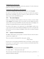
Figure 2: Number of start sites predicted at a specific distance from the annotation, using matrices
created with different number of isochores.
15
stop predicted at distance
12000
Hs
10000
Hs_1is
8000
Hs_2is
6000
Hs_4is
4000
Hs_47
Hs_6is
2000
Hs_8is
0
<= 0
<= 10
<= 25
<= 50
<= 100
> 100
missed
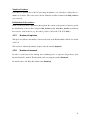
Figure 3: Number of stop sites predicted at a specific distance from the annotation, using matrices
created with different number of isochores.
As one matrix is created for each isochore, the amount of data necessary to build the matrices
increases with the number of isochores. It is advisable to use only one isochore to create the matrix
and, in case of trouble, to retry with a higher number of isochores.
16
7. Obtaining the matrices
Once the file has been written and saved, the three programs that calculate the matrices can be
executed.
The first program extract_mrna extracts the data from the files previously downloaded from the
FTP sites. The extraction is done taking the sequences that correspond to a species or to a higher
taxonomic level. Moreover, the program checks if the sequence is an mRNA and if the entire
coding sequence is contained in the sequence.
To launch the program, type into a terminal:
$ cd ESTScan
# where the scripts are
$ ./ extract_mrna sp.conf.
# sp.conf correspond to the configuration file you created
previously
The program extract_mrna will be executed using the file sp.conf. The script build_model_utils.pl
contained in the package enables the reading of the configuration files. The results will be stored in
the directory indicated in $datadir.
When the processing of the program is finished, “ sp.conf done” will appear in the terminal. This
information will appear after the execution of any script.
Then you have to use the second program which classifies the sequences into several groups. It is
possible to use the option -e with this script. This option is useful in cases where the matrices must
be evaluated, because it allows the splitting of the data into two groups : a training and a test set.
The splitting is necessary for the evaluation, because it is not particulary relevant to test the
discrimination power of the matrix on the same data as the data used for the training. If no option
is used, the training and test data will be the same. In addition the program splits the data from the
training set into several isochores and masks the redundant pieces of sequences. Finally, the
mRNAs are split into two files, one containing the coding part and the second containing the noncoding part.
17
To launch the program write:
$ ./prepare_mrna -e sp.conf
If you not need to evaluate the matrices, write only:
$ ./prepare_mrna sp.conf
Finally, you have to launch the third program that creates the codon usage table.
$ ./build_model sp.conf
18
8. Evaluation of the matrices
Once the matrices have been built, the user can evaluate their accuracy with the help of two
programs: extract_UG_est and evaluate_model.
Extract_UG_est searches UniGene clusters with an annotation making reference to the mRNA of
the test file previously created. It then does a megablast to know where the sequences match.
Finally based on the length of the match, its location and the mismatches, the program selects one
coding and another non coding sequence that matches an mRNA of the test file. These sequences
are used by the last script evaluate_model, which calculates the sensitivity and the specificity of
the matrices and also the accuracy to detect the start and stop sites. Furthermore, it produces some
histograms to illustrate the results.
$ cd ESTScan
# where the scripts are
$./extract_UG_est sp.conf
This step is time consuming.
Then you can launch the second program used for the evaluation: evaluate_model.
$ ./evaluate_model sp.conf.
The results appear in the shell and are also stored in your computer (see section 10).
19
9. Input and output of scripts
Each script has its own input and output files. In the following section, existing files will be
described.
9.1. Input and output of extract_mRNA
The script extract_mRNA expects files in Genbank or EMBL format [7, 11] (see section 12.1 and
12.2).
The output of this script is a file containing mRNA sequences in FASTA format with headers
containing: the accession number, annotation of coding sequence start and stop as two integers
values following the tag 'CDS:' and a description.
Example of sequence in FASTA format:
>tem|NM_014580 CDS: 46 1479 Homo sapiens solute carrier family 2, (facilitated glucose transporter) member 8
(SLC2A8), mRNA
GGCGGTTCAGGCGCCAGAGCTGGCCGATCGGCGTTGGCCGCCGACATGACGCCCGAGGACCCAGAGGA
AACCCAGCCGCTTCTGGGGCCTCCTGGCGGCAGCGCGCCCCGCGGCCGCCGCGTCTTCCTCGCCGCCTTC
GCCGCTGCCCTGGGCCCACTCAGCTTCGGCTTCGCGCTCGGCTACAGCTCCCCGGCCATCCCTAGCCTGC
AGCGCGCCGCGCCCCCGGCCCCGCGCCTGGACGACGCCGCCGCCTCCTGGTTCGGGGCTGTCGTGACCC
Description of the FASTA format:
A sequence in FASTA format begins with a greater-than (">") symbol immediately followed by
the identifier of the sequence and eventually followed by a description. After that, there are several
lines of sequence data. The sequence ends when another line starts with the ">" symbol, indicating
the start of another sequence, or at the end of the file.
9.2. Input and output of prepare_data
Prepare_data classifies mRNAs sequences, normally extracted from RefSeq or EMBL files by the
script extract_mRNA. However, it is possible to use a particular collection of mRNAs. In this case,
you must provide the data in FASTA format under the name of mRNA file: mrna.seq (where
extract_mRNA would store the extracted data). The header must contain annotations of coding
sequence start and stop in the header as two integer values following the tag 'CDS:'. The first
integer points to the first and the second integer to the last nucleotide of the CDS. Thus the length
20
of the CDS is <stop> - <start> + 1. The first nucleotide in the sequence has index 1 (see section
9.1).
The output of this script is mRNA data classified in several files: training and test set. Furthermore
the data from the training set is split according to its GC content. These files in FASTA format are
stored in the main directory and in the Isochores directory (see section 9.1). Two other files in
FASTA format are created and stored in the Evaluate directory. The first file contains the coding
part of the mRNAs (rnacds.seq) and the second contains the non-coding part (rnautr.seq).
9.3. Input and output of build_model
Build_model needs as input the mRNAs of the training set, always in FASTA format with the
annotation of the coding region in the header (see section 9.1 and 9.2). The sequences of the
training set can be taken from EMBL or RefSeq files if the scripts extract_mrna and prepare_data
have been used or from a particular collection of mRNAs in FASTA format.The output consists of
the matrices, one for each isochore, and which look like this:
FORMAT: hse_4is.conf CODING REGION 6 3 1 s C+G: 0 44
-1
0
2
-2
2
1
-8
0
1
0
1
-4
-1
-1
4
-3
0
-2
3
-2
3
0
-8
0
0
0
2
-1
-3
0
4
-2
2
-1
1
-3
3
1
-9
-1
9.4. Input and output of extract_UG_EST
The input of extract_UG_EST are the mRNA sequences of the test file (FASTA format) and the
UniGene clusters taken from the UniGene FTP site [15] (see section 12.3).
21
The output of this script includes two files containing the UTR part or the coding part of ESTs
(estutr.seq and estcds.seq respectively). These are in FASTA format. Three other files are created
during the execution of the script: ug.data which contains the information about the UniGene
clusters, clusters.lst which contains organized data of ug.data and matches.lst which contains the
information about the megablast done between the ESTs and the mRNAs (see section 12.4, 12.5,
12.6).
If during the use of the first script you have provided your own mRNAs, you also have to provide
ESTs with annotation in order to enable the evaluation. The annotation of the ESTs is possible
doing like extract_UG_EST. You can blast the ESTs against an mRNA to benefit from the
annotation of the mRNA in order to find out which part is coding or not, and divide the data into
two groups in the files estcds.seq and estutr.seq. Estutr.seq only contains non-coding nucleotides
whereas estcds.seq contains partially coding ESTs. For the sequences that are in the estcds.seq file,
it is necessary to indicate the location of the coding part (see section 9.1).
9.5. Input and output of evaluate_model
The execution of evaluate_model requires the following files:
-test.seq
-rnautr.seq
-rnacds.seq
-estutr.seq
-estcds.seq
-The matrices
All of the files except for the matrices are in FASTA format (see section 9.1). Estutr.seq and
nrautr.seq do not necessarily contain the tag 'CDS:' followed by the location of the coding
sequence, because all nucleotides may be non-coding.
The output is composed of many files, some containing sequences (ending with .seq), some ending
with “.dat”, containing data necessary to build gnuplot graphs. Other files end with “.gplot” and
are needed to create the graph easily and, finally, one file ends with “.R” containing the
information to draw a pie chart representing the percentage of start or stop sites that have been
found with a specific accuracy (see section 10). The most important file is stored in the report
directory and contains all the false positive and negative rates.
22
10. Results
10.1. Description of the results
The results are stored in the location indicated in the configuration file ($datadir). When the user
has launched the first script: extract_mrna, a directory is created for the species. This directory
contains several sub-directories: Evaluate, Isochores, Matrices, Report and Shuffled, as well as
a file called mrna.seq, which contains all the extracted mRNAs. Running prepare_data will add
two more files to the main directory: test.seq and training.seq.
The Evaluate sub-directory contains:
-
one file named 6_00030_0000001_4242_piecharts.R
-
Files containing sequences used during the evaluation (files ending with “.seq”).
-
Files ending with “.dat”, which contain the values to create some histograms.
-
Files ending with “gplot” that permit an easy output of histograms, because they contain all
the information needed (e.g. the title of the graph and the name of axes).
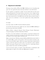
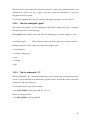
Examples of graphs that can be obtained with the files ending with gplot:
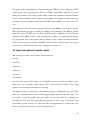
Figure 4: Distribution of distances between predicted and annotated start sites. Position zero is the
predicted start/stop site. Number (left) and percentage (right) of start sites predicted with a
particular accuracy.
23
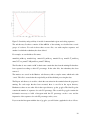
Figure 5: Sensitivity and specificity of models for untranslated regions and coding sequences.
The sub-directory Isochores contains all the mRNAs of the training set classified into several
groups of isochores. For each isochore there are two files, one with complete sequences and
another for which the redundancy has been deleted.
For example, we can find these file names:
mrna0-44_mr30.seq mrna0-44.seq mrna44-51_mr30.seq mrna44-51.seq mrna51-57_mr30.seq
mrna51-57.seq mrna57-100_mr30.seq mrna57-100.seq
The files that do not contain “mr30” in their name contain the data from the training file that have
been separated according to their GC percentage. In the other files, the redundancy has been
removed.
The matrices are stored in the Matrices sub-directory with a complex name, which ends with
“.smat”. This file is created after the script build_model has finished processing the data.
The Report sub-directory is useful to obtain the text written in the terminal when the program is
running. For each script that has been executed, there is one file in the report directory.
Furthermore, there are two other files in the report directory: gc.dat, gc.gplot. The first file gc.dat
contains the number of sequences for each CG percentage. The second file gc.gplot contains the
information necessary to build a histogram with the GC percentage on the x axes and the
frequencies of the sequences for each GC percentage on the y axes.
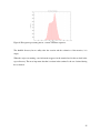
If you create the histogram with the data of gc.gplot, you will obtain a graph that looks as follows:
24
Figure 6: Histogram representing the GC content of human sequences.
The shuffled directory has no utility after the creation and the evaluation of the matrices, it is
empty.
When the scripts are running, some information appears in the terminal and is then stocked in the
report directory. The most important data that is written in the terminal is the one obtained during
the evaluation.
25
For example:
Using estscan to scan EST/mRNA
Evaluating new model on mRNA data using -m -100 -d -50 -i -50 -N 0....
⇐rate calculated on part
of mRNAs or ESTs
- predicting CDS for /export/scratch/ludi/ESTScan/Hse_4is/Evaluate/rnautr.seq...
found 44471302 coding of 176493655 nucleotides in 69999 of 335386 sequences
estimated false positive rate: 25.20% (nt) 20.87% (seq)
- predicting CDS for /export/scratch/ludi/ESTScan/Hse_4is/Evaluate/rnacds.seq...
found 180346838 coding of 182762167 nucleotides in 127695 of 167693 sequences
estimated false negative rate: 1.32% (nt) 23.85% (seq)
- predicting CDS on /export/scratch/ludi/ESTScan/Hse_4is/test.seq...
- computing histograms from
/export/scratch/ludi/ESTScan/Hse_4is/Evaluate/rnaprc6_00030_0000001_4242m100d50i50N0.seq...
predicted 159980 coding regions
estimated false positive rate 17.73% (nt)
⇐ rate calculated on complete mRNAs or ESTs
estimated false negative rate 2.47% (nt)
- writing data-files and gnuplot scripts...
start predicted at distance
<= 0:
45143
<= 10:
34804
<= 25:
8233
<= 50:
13089
<= 100:
19731
> 100:
38980
missed:
7713
stop predicted at distance
<= 0: 102436
<= 10:
3400
<= 25:
4445
<= 50:
8196
<= 100:
11503
> 100:
30000
missed:
7713
26
Four blocks like this one are written in the shell. The first two summarize the evaluation of the
matrix obtained on mRNAs, and the last two describe the evaluation obtained on ESTs (from
UniGene clusters). Moreover, if we focus on the results obtained on mRNAs or ESTs, we notice
that the second block reflects the analysis scanning the data (mRNAs or ESTs of UniGene clusters)
in one direction only, and the first block analyzing the data in both directions.
After the sentence: “computing histograms from” we have the false positive and negative rates
calculated on complete mRNAs or ESTs.
Finally, we can see the number of start sites followed by the number of stop sites, predicted at a
specific distance from the annotation.
This information is particulary important to get an idea of the precision for detecting the coding
region (sensitivity and specificity) and the accuracy of prediction of the start and stop site. These
numeric data help the user to determine if the matrix is good enough and then enable the results
obtained using ESTscan to be interpreted. Some graphical data is available, too; it helps to
visualize and understand the results (see section 10.2).
10.2. How to use the results
10.2.1.
The report’s files
All the information that appears in the terminal when the programs are running are stored in the
Report directory.
To see these files, go to the location you specified in $datadir and then enter the Report directory
using the command cd. Use the command ls to see the content of the directory, and then the
command less followed by the name of the file you are interested in to see the file.
Content of the report directory :
6_00030_0000001_4242_evaluate_model.log
6_00030_0000001_4242_prepare_data.log
6_00030_0000001_4242_extract_data.log
6_00030_0000001_4242_readconfig.log
6_00030_0000001_4242_extract_UG_EST.log
gc.gplot
6_00030_0000001_4242_generate_tables.log
gc.dat
27
The first six files represent the data obtained from the five scripts used to build the matrices and
evaluate them, and the last two, gc.gplot and gc.dat, contain the information to create the
histogram for the GC content.
To create the graph that shows the GC content use the gnuplot program (see section 10.2.2).
10.2.2.
The files ending with “gplot”
The creation of the graphs is possible with gnuplot [20]. The files ending with “.gplot” contain the
information necessary to draw the graph.
Write gnuplot in the terminal. At the end of the text which appears, just after “gnuplot >” write:
load “filename.gplot”
# Here, filename replaces the name of the file you want to visualize.
Saving the graph is possible using some commands in gnuplot, write:
> set terminal png
> set output “/tmp/gc.png”
> replot
> set output
> quit
10.2.3.
The file ending with “.R”
The file ending with “ .R ” contains the information to draw a pie chart representing the percentage
of start or stop sites that have been found with a specific accuracy. It draws the results stored in the
evaluate file of the report directory.
To obtain these charts, type into the terminal:
Cat 6_00030_0000001_4242_piecharts.R ¦ R -- no-save
Then to see the graph, write:
gv 6_00030_0000001_4242_piecharts.R.
28
11. Conclusion
The creation of the matrices is one of the first steps if you want to use ESTScan. This step is really
important since it determines all the results that will be obtained. Some parameters should be
optimized in order to develop reliable matrices.
Once the matrices are available for analysis, it is necessary to have a look at the sensitivity and
specificity of ESTScan using these matrices. These values reflect the capacity of ESTScan to
correctly classify sequences into the two groups: coding and non-coding. Thus these values allow
the results that will be obtained with ESTScan to be interpreted.
When we are able to use the matrices and understand their power, ESTScan can be launched on the
ESTs that must be analyzed. This type of analysis enables a better utilization of the information
contained in the ESTs. For example it allows the assessment of cDNA libraries that are subject to
contamination with genomic contaminants (non-coding). It can also lead to exon detection and
gene discovery.
29
12. Appendix
12.1. RefSeq format
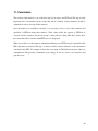
(b) Excerpt of a reviewed RefSeq nucleotide record. Note some of the revisions in annotation: the
official gene symbol and gene name defined by the Human Gene Nomenclature Committee; the
primary source of this sequence, links to OMIM and LocusLink, the brief gene description
(Summary), and the link to the RefSeq protein record [11].
30
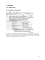
12.2. EMBL format
ID
XX
AC
XX
DT
DT
XX
DE
XX
KW
XX
OS
OC
OC
OC
XX
RN
RP
RX
RA
RT
RT
RL
XX
RN
RP
RA
RT
RL
RL
RL
XX
FH
FH
FT
FT
FT
FT
FT
FT
FT
FT
FT
FT
FT
FT
FT
FT
FT
FT
FT
FT
FT
FT
FT
FT
FT
FT
XX
SQ
X56734; SV 1; linear; mRNA; STD; PLN; 1859 BP.
X56734; S46826;
12-SEP-1991 (Rel. 29, Created)
25-NOV-2005 (Rel. 85, Last updated, Version 11)
Trifolium repens mRNA for non-cyanogenic beta-glucosidase
beta-glucosidase.
Trifolium repens (white clover)
Eukaryota; Viridiplantae; Streptophyta; Embryophyta; Tracheophyta;
Spermatophyta; Magnoliophyta; eudicotyledons; core eudicotyledons; rosids;
eurosids I; Fabales; Fabaceae; Papilionoideae; Trifolieae; Trifolium.
[5]
1-1859
PUBMED; 1907511.
Oxtoby E., Dunn M.A., Pancoro A., Hughes M.A.;
"Nucleotide and derived amino acid sequence of the cyanogenic
beta-glucosidase (linamarase) from white clover (Trifolium repens L.)";
Plant Mol. Biol. 17(2):209-219(1991).
[6]
1-1859
Hughes M.A.;
;
Submitted (19-NOV-1990) to the EMBL/GenBank/DDBJ databases.
Hughes M.A., University of Newcastle Upon Tyne, Medical School, Newcastle
Upon Tyne, NE2 4HH, UK
Key
Location/Qualifiers
source
1..1859
/organism="Trifolium repens"
/mol_type="mRNA"
/clone_lib="lambda gt10"
/clone="TRE361"
/tissue_type="leaves"
/db_xref="taxon:3899"
14..1495
/product="beta-glucosidase"
/EC_number="3.2.1.21"
/note="non-cyanogenic"
/db_xref="GOA:P26204"
/db_xref="InterPro:IPR001360"
/db_xref="UniProtKB/Swiss-Prot:P26204"
/protein_id="CAA40058.1"
/translation="MDFIVAIFALFVISSFTITSTNAVEASTLLDIGNLSRSSFPRGFI
FGAGSSAYQFEGAVNEGGRGPSIWDTFTHKYPEKIRDGSNADITVDQYHRYKEDVGIMK
DQNMDSYRFSISWPRILPKGKLSGGINHEGIKYYNNLINELLANGIQPFVTLFHWDLPQ
VLEDEYGGFLNSGVINDFRDYTDLCFKEFGDRVRYWSTLNEPWVFSNSGYALGTNAPGR
CSASNVAKPGDSGTGPYIVTHNQILAHAEAVHVYKTKYQAYQKGKIGITLVSNWLMPLD
..."
1..1859
/experiment="experimental evidence, no additional details
recorded"
CDS
mRNA
Sequence 1859 BP; 609
aaacaaacca aatatggatt
cacaattact tccacaaatg
tcggagcagt tttcctcgtg
A; 314 C; 355 G; 581 T; 0 other;
ttattgtagc catatttgct ctgtttgtta ttagctcatt
cagttgaagc ttctactctt cttgacatag gtaacctgag
gcttcatctt tggtgctgga …
60
120
180
//
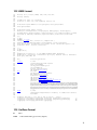
12.3. UniGene Format
ID
TITLE
Mm.1
S100 calcium binding protein A10 (calpactin)
31
GENE
S100a10
CYTOBAND
GENE_ID
3 F1-F2|3 41.7 cM
20194
LOCUSLINK 20194
EXPRESS
whole body; gastrointestinal tract; mixed; prostate; embryonic tissue; spleen; urinary; thymus; lymph
node; mammary gland; muscle; whole brain; endocrine; pancreas; uncharacterized tissue; bone marrow; female
genital; head and neck; extraembryonic tissue; eye; blood; brain; heart; liver; testis; limb; adipose tissue; lung;
sympathetic ganglion; connective tissue; dorsal root ganglion;
skin; inner ear
CHROMOSOME 3
STS
ACC=RH125510 UNISTS=162328
STS
ACC=M16465 UNISTS=178878
STS
ACC=RH124908 UNISTS=161730
STS
ACC=RH128467 UNISTS=211775
STS
ACC=S100a10 UNISTS=465493
PROTSIM
ORG=Homo sapiens; PROTGI=107251; PROTID=pir:JC1139; PCT=91; ALN=97
PROTSIM
ORG=Mus musculus; PROTGI=116487; PROTID=sp:P08207; PCT=100; ALN=97
PROTSIM
ORG=Rattus norvegicus; PROTGI=116489; PROTID=sp:P05943; PCT=94; ALN=94
SCOUNT
340
SEQUENCE
ACC=CA461262.1; NID=g24917614; CLONE=IMAGE:6754724; END=5'; LID=12110;
MGC=6677832; SEQTYPE=EST; TRACE=158140953
SEQUENCE
ACC=CB575716.1; NID=g29495246; CLONE=IMAGE:30295364; END=5'; LID=12733;
SEQTYPE=EST; TRACE=196933136
SEQUENCE
ACC=CB566164.1; NID=g29485694; CLONE=IMAGE:30294362; END=5'; LID=12615;
SEQTYPE=EST; TRACE=196939979
SEQUENCE
ACC=DV053483.1; NID=g76380766; CLONE=DLP01_06_N20; LID=18145; SEQTYPE=EST
SEQUENCE
ACC=DV060885.1; NID=g76388183; CLONE=NEONATAL_04_M20; LID=18147; SEQTYPE=EST
SEQUENCE
ACC=DV064402.1; NID=g76391700; CLONE=NEONATAL_22_E09; LID=18147; SEQTYPE=EST
SEQUENCE
ACC=DV066639.1; NID=g76393937; CLONE=UGS01_04_L15; LID=18148; SEQTYPE=EST
SEQUENCE
ACC=DV055636.1; NID=g76382938; CLONE=DLP01_15_A03; LID=18145; SEQTYPE=EST
//
32
12.4. Example of ug.data file:
ID
Hs.100043
TITLE
Coiled-coil domain containing 124
GENE
CCDC124
CYTOBAND
GENE_ID
19p13.11
115098
LOCUSLINK 115098
HOMOL
YES
EXPRESS brain; lung; skin; colon; eye; mixed; whole body; placenta; embryonic tissue; connective tissue; larynx;
uncharacterized tissue; bone; whole brain;
pharynx; salivary gland; lymph; muscle; uterus; spleen; ovary; blood; liver; parathyroid; heart; testis; mammary gland;
lymph node; kidney; prostate; mouth; pancreas; cervix
CHROMOSOME 19
STS
ACC=RH93753 UNISTS=84827
STS
ACC=RH46130 UNISTS=88276
PROTSIM
ORG=Arabidopsis thaliana; PROTGI=18394335; PROTID=ref:NP_563993.1; PCT=33.04; ALN=216
PROTSIM
ALN=221
ORG=Caenorhabditis elegans; PROTGI=17510611; PROTID=ref:NP_490873.1; PCT=50.43;
PROTSIM
ORG=Homo sapiens; PROTGI=1070603; PROTID=pir:CGHU7L; PCT=29.64; ALN=263
PROTSIM
ORG=Mus musculus; PROTGI=5921190; PROTID=sp:P08121; PCT=28.37; ALN=263
SCOUNT
261
SEQUENCE ACC=BM554853.1; NID=g18794811; CLONE=IMAGE:5468925; END=5'; LID=8775;
MGC=34147541; SEQTYPE=EST; TRACE=115579612
SEQUENCE ACC=BU539378.1; NID=g22849819; CLONE=IMAGE:6570116; END=5'; LID=10554;
MGC=34147541; SEQTYPE=EST; TRACE=158255138
SEQUENCE ACC=BM558432.1; NID=g18801173; CLONE=IMAGE:5476590; END=5'; LID=8775;
MGC=34147541; SEQTYPE=EST; TRACE=115580613
SEQUENCE ACC=BQ883763.1; NID=g22275771; CLONE=IMAGE:6291297; END=5'; LID=7269;
MGC=34147541; SEQTYPE=EST; TRACE=142965156
estcds.seq
>emb|BM912135|BM912135.1 CDS: 12 565 [Homo sapiens]AGENCOURT_6613231 NIH_MGC_41 Homo sapiens
cDNA clone IMAGE:5473631 5', mRNA sequence. (first 565 nucleotides)
CCTGCTGAGGGATGCCCAAGAAGTTCCAGGGTGAGAACACCAAGTCGGCAGCGGCCCGGGCACGTAGG
GCAGAGGCCAAGGCGGCCGCTGATGCCAAGAAGCAGAAGGAGCTGGAGGATGCCTACTGGAAGGACGA
CGACAAACACGTCATGAGGAAGGAGCAGCGCAAGGAGGAGAAGGAGAAGCGGCGCCTCGACCAGCTG
GAACGTAAGAAGGAGACGCAGCGCCTACTGGAGGAGGAGGACTCCAAGCTCAAGGGCGGCAAGGCGCC
GCGGGTGGCCACGTCCAGCAAGGTCACCCGGGCCCAGATCGAGGACACGCTGCGCCGAGACCATCAGCT
CAGGGAGGCCCCGGACACAGCCGAGAAAGCCAAGAGCCATCTGGAGGTGCCGCTGGAGGAGAACGTGA
ACCGCCGCGTGCTGGAGGAGGGCAGCGTGGAGGCGCGCACCATCGAGGACGCCATTGCAGTGCTCAGC
GTGGCGGAGGAGGCGGCCGACCCGGCCCCAGAAAGACGCATGCGGGCACCCCTTCCCCGCTTTCAGGAA
CACCATCTGCCGCGGTTCAA
33
12.5. Example of cluster.lst file
rs:NM_138442 : embl:BM554853 embl:BU539378 embl:BM558432 embl:BQ883763
embl:BM912135 embl:BQ878175 embl:BM554613 embl:BM810865 embl:BM913379
embl:BE733510
embl:BM551615
embl:BQ071416
embl:BQ052057
embl:BM558385
embl:BQ889758 embl:BM811068 embl:BM915137 embl:BM914662 embl:BM915698
12.6. Example of matches.lst file
rs:NM_138442 108 779 embl:BM913379 97 948 11 31
rs:NM_138442 108 779 embl:BE733510 191 947 1 10
rs:NM_138442 108 779 embl:BQ071416 97 853 4 25
rs:NM_138442 108 779 embl:BQ052057 98 975 21 42
rs:NM_138442 108 779 embl:BM558385 97 1039 12 31
rs:NM_138442 108 779 embl:BQ889758 97 723 4 17
rs:NM_138442 108 779 embl:BM811068 97 773 24 33
rs:NM_138442 108 779 embl:BM915137 97 993 22 38
rs:NM_138442 108 779 embl:BM914662 97 1026 11 34
rs:NM_138442 108 779 embl:BM915698 97 985 22 36
rs:NM_138442 108 779 embl:BQ062920 97 975 17 39
34
13. References
[1]
Bernardi, G. 1989. The isochore organization of the human genome. Annu. Rev. Genet.
1989.23:637-659.
[2]
Borodovsky, M. Y. and J. D. McIninch 1993. GENMARK: parallel gene recognition for both
DNA strands. Comput. Chem. 17: 123-133.
[3]
Burge, C. and S. Karlin 1997. Prediction of complete gene structures in human genomic
DNA. Journal of Molecular Biology 268(1): 78-94.
[4]
Costantini, M., Clay, O., Auletta, F., Bernardi, G. 2006. An isochore map of human
chromosomes. Genome Res. Apr;16(4):536-41
[5]
Durbin, R., S. Eddy, A. Krogh, and G. Mitchison. Biological sequence analysis –
Probabilistic models of proteins and nucleic acids . Cambridge University Press, 1998.
[6]
Iseli, C., C. Victor Jongeneel, Philipp Bucher, 1999. ESTScan: a program for detecting,
evaluating, and reconstructing potential coding regions in EST sequences. In Intelligent
Systems for Molecular Biology, pages 138_148, Heidelberg, Germany, August 1999. AAAI
Press.
[7]
Kanz, C, P Aldebert, N Althorpe, W Baker, A Baldwin, K Bates, P Browne, A van den
Broek, M Castro, G Cochrane, K Duggan, R Eberhardt, N Faruque, J Gamble, F Garcia Diez,
N Harte, T Kulikova, Q Lin, V Lombard, R Lopez, R Mancuso, M McHale, F Nardone, V
Silventoinen, S Sobhany, P Stoehr, MA Tuli, K Tzouvara, R Vaughan, D Wu, W Zhu and R
Apweiler. The EMBL Nucleotide Sequence Database. Nucleic Acids Research, 2005, Vol.
33, Database issue
[8]
Lottaz, C, Iseli C, Jongeneel CV, Bucher P. (2003) Modeling sequencing errors by
combining Hidden Markov models. Bioinformatics 19, 103-112
[9]
Lottaz, C. 2002. Master’s thesis in bioinformatics: Modelling expressed sequence Tags with
a hidden markov model (http://estscan.sourceforge.net/).
[10] Pearson, W. R. Searching protein sequence libraries: comparison of the sensitivity and
specificity of the smith-waterman and FASTA algorithms. Genomics, 11(3):635_650,
November 1991.
[11] Pruitt KD, Katz KZ, Sicotte H, Maglott DR. 2000. Introducing RefSeq and LocusLink:
curated human genome resources at the NCBI. Trends Genet 16(1):44-7.
35
[12] Wheeler, DL., T Barrett, DA. Benson, SH. Bryant, K Canese, V Chetvernin, DM. Church,
M, R Edgar, S Federhen, LY. Geer, W Helmberg, Y Kapustin, DL. Kenton, O Khovayko,
DJ. Lipman, TL. Madden, DR. Maglott, J Ostell, KD. Pruitt, GD. Schuler, LM. Schriml, E
Sequeira, ST. Sherry, K Sirotkin, A Souvorov, G Starchenko, TO. Suzek, R Tatusov, TA.
Tatusova, L Wagner and E Yaschenko. Database resources of the National Center for
Biotechnology Information. Nucleic Acids Research, 2006, Vol. 34, Database issue D173–
D180 doi:10.1093/nar/gkj158
[13] Zhang,Z., Schwartz,S., Wagner,L. and Miller,W. (2000) A greedyalgorithm for aligning
DNA sequences. J. Comput. Biol., 7, 203–214.
14. Web site references
[14]
http://www.ncbi.nlm.nih.gov
[15]
http://www.ncbi.nlm.nih.gov/UniGene
[16]
http://www.ebi.ac.uk/
[17]
http://sourceforge.net/projects/estscan/
[18]
http://estscan.sourceforge.net/
[19]
http://fedora.redhat.com/
[20]
http://www.gnuplot.info/
[21]
http://www.ncbi.nlm.nih.gov/Taxonomy/
36