Download GeoLing user guide

user guide
version 1.0
22nd September 2014
“Neue Dialektometrie mit Methoden der stochastischen Bildanalyse”
DFG-financed project (2008-2014)
Stephan Elspaß
Henrik Hassfeld
Werner König
Daniel Meschenmoser
Simon Pickl
Simon Pröll
Jonas Rumpf
Volker Schmidt
Aaron Spettl
Evgeny Spodarev
Julius Vogelbacher
Raphael Wimmer
http://www.geoling.net/
table of contents
table of contents ........................................................................................................................................... 2
acknowledgements ....................................................................................................................................... 2
license and terms of useage ......................................................................................................................... 2
I.
basics ...................................................................................................................................................... 3
I.1
what is GeoLing and what does it do? ........................................................................................ 3
I.2
download and installation ........................................................................................................... 3
I.3
starting GeoLing ............................................................................................................................ 3
I.4
entering your data ........................................................................................................................ 4
I.5
customizing and expanding the program ............................................................................... 14
II.
program functions ......................................................................................................................... 15
II.1
map browser ............................................................................................................................... 16
II.2
intensity estimation .................................................................................................................... 16
II.3
group browser ............................................................................................................................ 21
II.4
export........................................................................................................................................... 21
II.5
factor analysis ............................................................................................................................. 22
II.6
cluster analysis ............................................................................................................................ 26
III.
references ........................................................................................................................................ 26
acknowledgements
GeoLing – along with this accompanying manual – was written as a part of the project Neue
Dialektometrie mit Methoden der stochastischen Bildanalyse (“new dialectometry using methods of
stochastic image analysis”), financed by the Deutsche Forschungsgemeinschaft (DFG) between
2008 and 2014. All work has been carried out by people associated with three institutions:
- Institute of Stochastics (Ulm University)
- Lehrstuhl für Deutsche Sprachwissenschaft (University of Augsburg)
- Germanistische Sprachwissenschaft (University of Salzburg)
license and terms of useage
This software is licensed under the GNU General Public License v 3.0 (published on 29 June
2007). The full text of GPL 3 is available at https://www.gnu.org/licenses/gpl-3.0.
2
Although we took reasonable precautions and conducted extensive testing, we would like to
stress that the software comes without any warranty or guarantee.
I.
I.1
basics
what is GeoLing and what does it do?
In short, GeoLing is a handy tool for performing statistical analyses on spatial data: You can use
data from dialect surveys, transform them into smoothed maps (via density estimation), detect
structures that run through the data and find groups of maps that share spatial features.
We developed this program with linguistic applications in mind, but that should not stop you
from using it for any kind of spatially conditioned data.
I.2
download and installation
The software is written in Java – as Java runs on multiple platforms, there is one version for all
users. Please make sure that the Java version running on your machine is up to date; updates are
obtainable on http://www.java.com. The latest version of GeoLing and this accompanying guide
are available for download at http://www.geoling.net/ as an archive file (geoling.zip). Note that
GeoLing requires at least 2 GB RAM, furthermore we recommend a dual-core processor.
GeoLing is ready to use after unzipping the archive file (geoling.zip); no installation is required. It is
important that GeoLing has full access to its own directory. This will be the case by default if you
extract GeoLing somewhere in your own home directory. (In particular, write-access to the
“properties” and “databases” subdirectories is required.)
Originally, the software was developed for and tested on the data of the Sprachatlas von BayerischSchwaben (SBS).1 The corresponding database (that served as basis for most examples in this
documentation as well) is supplied for demonstration purposes.
I.3
starting GeoLing
The program starts by executing the file geoling.jar.
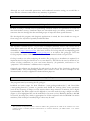
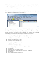
Included are batch scripts for both Windows (“start-geoling-windows.vbs”) and Linux/Mac
(“start-geoling-linux.sh”) systems to provide more RAM for GeoLing. Since some operations
(such as the clustering of maps, see II.6) require relative large amounts of memory, this is highly
recommended. The batch scripts can be adapted to your own needs by using a simple text editor
(Figure 1). The highlighted line can be modified to use more (or less) RAM. By default, 1400 MB
are used as Java heap size, which is appropriate for 32-bit computers with 2 GB RAM. On 64-bit
machines (with 64-bit Java installed) larger values may be used.
1
The Sprachatlas von Bayerisch-Schwaben is based on dialect data gathered in the 1980s in the transient area of the
political regions of Swabia, Bavaria and Franconia in southern Germany (see SBS Volume 1 for further
information).
3
Figure 1: Batch script for running GeoLing with more RAM on a Windows platform.
I.4
entering your data
GeoLing requires all data to be in the form of a SQL database. You can either set up a database
running on a local server yourself or use the program’s built-in options to let it set one up for
you. Both options will be outlined in the following passages.
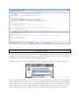
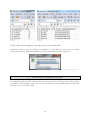
In either case, choose “Create new database” in the “Database” dialogue on startup (Figure 2).
Figure 2: Creating a new database.
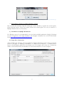
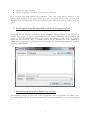
The following dialogue box (Figure 3) allows choosing between both options: Using a database
that is running on a separate server or using a stripped-down built-in database management
system. While the first option offers higher speed and usability in a network situation, it is only
recommended for users with prior knowledge of database systems. The second one is easier to
use for novices, but leads to slightly slower performance of GeoLing and is limited to local use.
4
Figure 3: Choosing the database type.
 First option: setting up a SQL database yourself
We start with the necessary steps for setting up a server. Should you prefer the second option,
please skip this section. (If you are unsure, choose the second option. It is easy to switch to a
MySQL database later on, if necessary.)
a) Installation of MySQL Workbench
For Windows users it is recommended to use the freely available application MySQL Workbench
for the management of the SQL databases. The MySQL Community Server can be downloaded
from http://dev.mysql.com/downloads/mysql/.
b) Setup New Connection
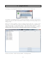
After installing the software, start the application MySQL Workbench 6.0 CE. Click on the plus
button to the right of “MySQL Connections” to “Setup New Connection”. A window like in
Figure 4 should appear; please fill in the blanks as in our example. (Of course, the “Connection
Name” can be chosen freely. We decided on “IceCreamConnection” for our example.)
Figure 4: Setting up a new connection in MySQL.
5
If all values have been entered correctly, a click on the button “Test Connection” should yield the
message “Connection parameters are correct”. Then, click on “OK” and you will see the new
connection in MySQL Workbench.
c) Create a new schema in the connected server
Click on the new connection and a new view appears. On the left, you can see a navigator bar
containing some exemplary schemas. Click on the symbol “Create a schema in the connected
server”, which shows two disks (marked yellow in Figure 5).
Figure 5: Creating a new schema in MySQL.
Enter a name (e.g. icecream) for the new schema and click “Apply”. Then, click on the symbol
“Data Import/Restore”. In the window which opens next, choose the toggle button “Import
from Self-Contained File” and choose the path to the file “dialectometry.sql”, which contains the
create-statements for the tables. Then, select the “Default Schema to be Imported to” (e.g.
icecream) and click on “Start Import”. After the import has been finished, a click on the new
schema should reveal the following tables (in brackets: the names of the columns):
 bandwidths (id, map_id, weights_identification, kernel_identification,
distance_identification, estimator_identification, bandwidth)
 border_coordinates (id, border_id, order_index, latitude, longitude)
 borders (id, name)
 categories (id, parent_id, lft, rgt, name)
 categories_maps (id, category_id, map_id)
 configuration_options (id, name, value)
 distances (id, name, type, identification)
 groups (id, name)
 groups_maps (id, group_id, map_id)
 informants (id, location_id, name)
 interview_answers (id, interviewer_id, informant_id, variant_id)
 interviewers (id, name)
 levels (id, name)
 locations (id, name, code, latitude, longitude)
 location_distances (id, distance_id, location_id1, location_id2, distance)
 maps (id, name)
 tags (id, parent_type, parent_id, name, value)
6


variants (id, map_id, name)
variants_mappings (id, variant_id, level_id, to_variant_id)
If all 19 tables have been created, the installation of the local server and the creation of the
required SQL database in the given format have been successful. Please make sure that your
MySQL Server is running after every restart of your system. Otherwise, GeoLing cannot access the
server.
 Second option: using GeoLing’s built-in database management system
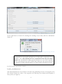
On startup, choose “Create new database” in the “Database” dialogue (Figure 2) and “SQLite” as
database type (Figure 3). You are then prompted to set location and name for the database file
(Figure 6). The filename should follow the pattern databasename.db (make sure you explicitly
specify the file extension “.db”). A suitable location for the database file is the subdirectory
“databases” located in the GeoLing directory. For example, the included SBS database is stored in
“databases/SBS/SBS.db”.
Figure 6: Specifying location and name of the database file.
 After setting up the database: import your own data
The following passages outline each of the original files that are necessary for import. They
should all be placed in one folder. Press the button “Choose input folder” to set its path (Figure
7).
7
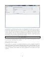
Figure 7: Window for data import in GeoLing.
To the right there is a button for selecting the encoding of your data, UTF-8 or ISO-8859-1
(Figure 8).
Figure 8: Choosing the encoding of the data.
NB: GeoLing uses a decimal point (".") as a decimal mark, not a comma. There is
no separator for thousands. All tables are csv-files with a semicolon (";") as
delimiter – thus, there should never be a semicolon in the data you wish to
import. We recommend avoiding special characters in your data if possible,
because this eliminates the need to think about characters with special meanings
or character encodings (like ISO-8859-1 or UTF-8) during data import/export.
Let’s look at the specific files in detail:
border_coordinates.csv
This table determines the outer border of the basic map, delimiting the area of investigation. The
first column features the order of the waypoints; the following ones latitude and longitude of
these points (see Figure 9).
8
Figure 9: border_coordinates.csv.
NB: It is possible to define more than one outer border; thus, you will be asked
to specify a name for each border.
locations.csv
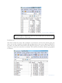
This table contains the names and coordinates of all locations, with the first column giving the
name, the second an identifier (number/ID-tag/abbreviation) (that can be displayed directly in
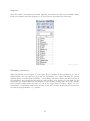
the maps), the third and fourth latitude and longitude (Figure 10). Note that the name must be
unique, it is used in the other files as reference. All locations should have different geographical
coordinates.
Figure 10: locations.csv.
9
maps.csv
Here, the names of all maps are recorded. Typically, this will be the same as the variable’s name.
Only one column is necessary (Figure 11). As for locations, the name has to be unique.
Figure 11: maps.csv.
informant_answers.csv
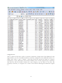
This will probably be the largest of your source files: It bundles all the information (in case of
dialectological uses all responses given by the informants) in a table following the pattern
informant (rows) x variables/maps (columns) = record (fields). The first column contains the name of
the informant, the second one the location (same spelling as in locations.csv), the third one the
interviewer (or similar additional information on the record). Starting with the fourth column,
each column’s header bears the name of one of the maps listed in maps.csv (Figure 12). If a
combination of informant and location features more than one record, they can be entered into
the same field, separated by a “|” symbol.
10
Figure 12: informant_answers.csv.
categories.txt
This is a plain text file that is used to construct a hierarchy of maps that is later displayed in the
map browser (see II.1). Possible hierarchies would for example be the traditional system of a
dialect atlas: volumes > topics > subtopics > single maps. Each line contains the name of a category,
followed by a colon, followed by all its direct children, each of them separated by a semicolon.
The first line after the header contains the “top” category, e.g. the name of the atlas. The
hierarchy is recursive, i.e. categories on a “lower” level can have subcategories themselves (Figure
13.
11
Figure 13: categories.txt.
categories_maps.txt
Each map has to be assigned to a category to be visible and accessible in the GUI. This allocation
is taken care of through the entries in categories_maps.txt. The basic principle follows the one
above: Each line features a category, followed by a colon, and all maps that are to be assigned to
the category. These maps are again separated from each other by a semicolon (Figure 14).
Figure 14: categories_maps.txt.
groups_maps.txt
This third plain text file can be used to simplify analyses by providing ready-made groups of
maps in the GUI (for example all maps containing fronted vowels). The difference of categories
and groups is that categories are hierarchical and for selecting individual maps in the GUI, but
groups are sets of maps which are used later on for analyses based on a sub-corpus. Principle and
execution follow the other two text files above. This function is not mandatory for a successful
import; groups can be generated from within the GUI as well (see II.3).
NB: It is essential to end all lines – also the last one – of these three plain text
files with a line break; otherwise the import routine will ignore their content.
distances.csv
GeoLing is able to calculate the geographic distances between the locations based on the
coordinates you provided in locations.csv. Nevertheless you are free to enter your own distance
measures (e.g. travel time) using distances.csv. Figure 15 displays the way the distance values should
be arranged.
12
Figure 15: distances.csv.
As last steps, the functions “Prepare variant mapping” and “Read variant mapping” are used to
generate levels of abstraction or granularity over the base layer: For example, the data might
contain complex phonetic transcriptions for every record, but you intend to use the data to draw
a map on phonological or on purely lexical variation. You could then create a level of abstraction,
where various raw phonetic values are mapped to a few phonological values – and another level
where you disregard phonetic/phonological detail completely and focus on lexical differences
instead.2 “Prepare variant mapping” outputs a CSV table for every map that contains all variants
(and their count) that are contained in the data (Figure 16). This file can be edited and then be
imported again. Each additional column may contain one individual abstraction (see Figure 17 for
a basic example with just one level). Should you not need any abstraction at all, it is sufficient to
simply copy the first column and insert it as the third.
2
Or, you might just use it to handle misspellings in the data.
13
Figure 17: Mapping with one level of abstraction.
Figure 16: Empty csv for mapping.
Finally, “Read variant mapping” reads and processes these edited tables.
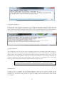
Should you wish to revise or enlarge your database at a later time, you can access the editing
process by choosing “Edit existing database” during the startup selections (Figure 18).
Figure 18: Editing an existing database.
I.5
customizing and expanding the program
In compliance with the GPL 3 license, the entire source code for GeoLing is part of the package
provided on the homepage. Thus, you can not only add your own program parts but tweak the
existing ones to your exact needs.
14
II.
program functions
On startup, you are prompted for the database you want to work with (Figure 19).
Figure 19: Database selection.
The database for the SBS (Sprachatlas von Bayerisch-Schwaben) is included for demonstration
purposes. You may also create a new database or edit an existing one from this prompt (see I.4,
entering your data).
When you’ve chosen a database, a screen as in Figure 20 opens. Three tabs – Categories, Groups
and Export – are accessible in the top left of the window, three buttons on the right bottom –
“Open selected map…”, “Open factor analysis…” and “Open cluster analysis…” – can be
clicked to open further tabs. Each of those tabs contains one way of accessing, visualizing or
analyzing the data. All of these tabs are explained in detail through the next paragraphs.
Figure 20: Startup screen.
The tab to the far left – which is active by default – is the map browser.
15
II.1 map browser
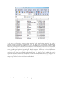
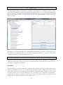
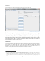
The map browser displays the datasets contained in the database. For example, Figure 21 shows
part of the SBS database structure: Just like in the printed form of the atlas, the data is subdivided
into 13 volumes, and each of these volumes is subdivided into categories of maps. The map
browser reflects this structure. Navigation through the tree enables the user to access each single
dataset or “map”.
Figure 21: Map browser.
Highlighting an entry (as in Figure 21) reveals additional information about it in the right half of
the window; a double click on it (or the button “Open selected map…”) opens a tab named
“density estimation” for generating a density map.
II.2 intensity estimation
This tab contains the means to transform the discrete point data of the map you clicked into
graded area class maps. Before we get into the technical details, it might be wise to take a look at
why doing so might be a good idea.
Motivation
The motivation for intensity estimation of dialect data stems from the issues introduced in data
collecting: All dialect data we survey are merely statistical samples. While dialectologists have
always done their best in controlling for unwanted bias and putting great emphasis on the choice
of subjects, there can be no doubt that there is no such thing as an “maximally representative”
sample. But drawing conventional point-symbol maps from data sampled at isolated points
suggests this nonetheless; graded area class maps do not.
16
If we acknowledge that our data are statistical samples, we must acknowledge that they contain a
margin of error. Consider that we asked another person, consider that we asked more persons
overall, consider that we asked the same persons on another day and in a different state of mind,
etc. To compensate for this, we can assign a certain probability to every one of the data points –
the intensity – and map that instead of the original samples. To estimate this individual
probability, we take into account the surrounding data points since proximity often entails
linguistic similarity. (We will have to define what exactly we talk about when we talk about
“proximity”, however. As will be explained, we use distance measures for this.) Thus, maps
generated employing intensity estimation are not only eye candy but offer a probabilistic view on
the underlying data.3 This is a reinterpretation of the data, not a modification: In intensity
estimation, the “weight” of a data point is not altered, but is “smeared” across a certain ambit.
Note that sometimes we say “density estimation” instead of “intensity estimation”. This is exactly
the same – “density” comes from the statistical background, “intensity” is closer to the
interpretation.
Parameters
With this in mind, we can return to the program’s GUI. Figure 22 shows the tab for intensity
estimation, where different parameters can be selected using check boxes and drop-down menus.
These parameters are used to perform a so-called “kernel density estimation” to estimate the
intensities.
Figure 22: Tab for density estimation
3
RUMPF / PICKL / ELSPAß / KÖNIG / SCHMIDT (2009) explain the whole process in full detail. Some applications
are documented by RUMPF (2010), PICKL / RUMPF (2011, 2012), PICKL (2013a, b) and PRÖLL (2013a, b).
SCHERRER (2011) and SCHERRER / RAMBOW (2010a, b) use this approach for automatic dialect translation
systems.
17
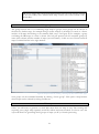
Let’s look at them from top to bottom:
parameter
Level
Distance
Plotting type
Kernel
Automatic bandwidth
Manual bandwidth
description
This drop-down menu sets the level of abstraction or “granularity”. For
the SBS database, we used these levels to disregard phonetic or
morphological details that would be over-informative for certain questions.
PICKL (2013b: 75–78) covers this thoroughly.
Here, the type of distance measure between locations has to be selected.
The SBS database features geographic and linguistic distances;4 you can
easily integrate your own distances (see I.4).
There are two types of maps that can be generated. One type subdivides
the mapping space into Voronoi cells; every point of the area is assigned to
the nearest point of measurement. The other one is continuous; it
interpolates each value on a dense grid (only for geographic distances, see
PRÖLL 2013b: 58–64 for more details).
This is for choosing the kernel (Gauss, K3 or Epanechnikov), which is
used in kernel density estimation. In principle, the choice of kernel is not
as relevant for the result as other parameters (see JANERT 2010: 20 in
general or RUMPF 2010: 49–63 for our data). Still, it can have an effect.
These options select one of three methods for optimizing the bandwidth,
which controls the range of the distance-dependent smoothing:
- LCV (likelihood cross-validation)
- LSCV (least-squares cross-validation)
- Min-C-Max-L, an algorithm that minimizes cost between two
concurring statistical parameters of the map (see PICKL 2013a for
details).
This lets you choose a bandwidth manually by entering a numeric value; it
overrides the choices made in the field for automatic bandwidth above.
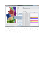
Visualization
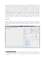
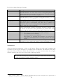
After choosing the parameters, a click on the button “Draw area class map” computes and
visualizes the data. Figure 23 displays an example from the SBS data. The different colour hues
represent different dominant variants. By “dominant” we mean that the variant has a higher
intensity (density) than every one of the locally competing variants.
NB: Point the mouse to any location on the map to obtain more information in
a tooltip (e.g. name of location, intensity values).
4
PICKL / SPETTL / PRÖLL / ELSPAß / KÖNIG / SCHMIDT (2014) provide a comparison of the performance of
geographic and linguistic distances in intensity estimation.
18
Figure 23: Display of an area class map.
Spatial characteristics
The values displayed between the parameters and the buttons are three spatial characteristics
established in RUMPF / PICKL / ELSPAß / KÖNIG / SCHMIDT (2009):
- total border length in kilometers, or complexity
- overall area compactness and
- overall homogeneity
The uses of these values are manifold: PICKL (2013a,b) and PRÖLL (2013b) show only some of
the possible interpretations that arise from statistical tests performed on these values and their
differences across maps.
Export
Export options are available through a click on “Save map”. This opens a dialogue that allows to
export the map itself to an Encapsulated PostScript (*.eps) file or a Portable Network Graphics
(*.png) file, but also the intensity values in the form of an Extensive Markup Language (*.xml)
file.
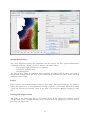
Dealing with single variants
The fields to the lower right side of the window show all the variants the currently viewed
variable/map contains. Double-clicking on one of them allows for changing its colour in the area
class map (see Figure 24).
19
Figure 24: Changing the colour of a variant.
With just a single click on the variant and another one on “Draw variant map”, one can visualize
a map of the density of just this single variant (be it dominant in the area class map or not). The
colour of these maps is blue by default (see Figure 25).
Figure 25: Display of a single variant.
20
NB: If you single click on the right-hand column (the one with colours) instead
of the left column, then “Draw variant map” will use this colour instead of the
default blue.
II.3 group browser
The group browser tab is for combining single maps to groups; these groups can be chosen as
the basis for further steps, for example doing a cluster analysis on all maps of vowels or a factor
analysis of all maps that belong to the semantic field “crop”. In Figure 26, for example, a group
containing all SBS maps on verbs is shown. The left part presents all the accessible groups by
name (first column) and the number of maps (second column). A click on one of them reveals all
maps contained therein in the right window.
Figure 26: Group browser tab, featuring a selected group (left) and its content (right).
New groups can be assembled manually by clicking “Create group”. This opens a map browser
where maps can be selected by ticking checkboxes.
II.4 export
Often, you will want to generate or work with more than one map at once. But creating and
exporting every single map separately would be tedious and uneconomical. For those cases the
export tab allows for generating whole groups of maps (see II.3) via batch processing.
21
Figure 27: Export tab.
You can choose a pre-defined group of maps, select the parameters the same way as it’s done in
the calculation of single maps (see II.2) and set an output directory; the process then generates an
EPS file and a PNG file containing the map as well as an XML file containing the resulting
intensity values for each of the maps in the chosen group. In addition to that, it outputs a CSV
(Comma Separated Value) file (easily interpretable by a broad selection of consumer software)
that contains a list of all maps in the group, their respective complexity, overall compactness and
overall homogeneity, as well as the number of dominant variants.
II.5 factor analysis
The second of the tabs accessible via button on the startup screen (cf. the beginning of section
II) opens a tab for performing a factor analysis.
Background on factor analysis
Factor analysis is a technique for reducing the dimensions in data (originally developed for
application in psychology, see e.g. WOTTAWA 1996: 813). It can be used for finding “traits” that
run through the data, a small number of underlying patterns that can describe large parts of the
overt variation in a compact way. To our knowledge, WERLEN (1984) was the first to use factor
analysis in a variationist context; BIBER (1985, 1991) popularized its use by applying it in corpus
linguistics.
22
Parameters
Three parameters are directly accessible through the GUI (see Figure 28):
Figure 28: Factor analysis, basic mask.
The first one is – again – the abstraction level. For factor analysis, we recommend using an
abstraction level as low as possible (e.g. level 1). The menu for “Group” lets you choose any of
the groups of maps you specified in the group tab (II.3). The checkbox options deal with the
number of factors that will be extracted from the data. There is a consensus that there is no right
or wrong number of factors; nevertheless, methods for optimizing the number of factors have
been developed and used for many years. We implemented the Kaiser criterion5, which is a widely
used standard criterion. Still, it is possible to disregard the Kaiser criterion and set the number of
factors manually by entering it in the text box.6
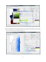
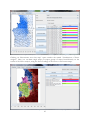
Visualization
A click on the button “Draw factor map” starts the calculation of the factors. Figure 29 shows a
typical result of an analysis like this, a factor map of all SBS maps dealing with nominal
morphology. As always, the map has a mouse-over function: If you point the mouse to any
location, a tooltip will reveal the local composition and interplay of factors.
5
6
The Kaiser criterion disregards factors with an eigenvalue smaller than 1.
In general, the Kaiser criterion is seen as a rather conservative approach that yields results with relatively high
numbers of quite weak factors. However, our applications (PICKL 2013b, PRÖLL 2013, PRÖLL / PICKL / SPETTL
to appear) could show that even those small factors are reasonably interpretable from a geolinguistic point of
view.
23
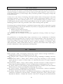
Figure 29: Example: Factor analysis of SBS maps featuring nominal morphology.
On the right side, a list with all the extracted factors appears, each giving the percentage of the
overall variation it represents. The buttons “Save results” and “Save map” open save dialogues
for exporting XML and EPS files of the analyses. As seen with the variants in density estimation
(II.2), if you select one of the factors in this list and click “Show factor loading”, the drawing area
visualizes this factor individually (Figure 30).
24
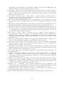
Figure 30: Example: Factor analysis of SBS maps featuring nominal morphology, display of single factor.
Clicking on “Reconstruct area class map” opens another tab named “Visualization of factor
weights”. Here, you can draw single maps (or export groups of maps) based directly on the
results of the factor analysis, using the factor loadings of all factors to reconstruct maps.
Figure 31: Reconstruction of an area class map using results of factor analysis.
25
II.6 cluster analysis
This tab provides the means for clustering. While clustering in general long since has become a
common technique in dialectometry, the way GeoLing uses cluster analysis is new: It does not
cluster dialects/locations, it clusters maps. Thus, it becomes possible to find groups of maps that
are spatially similar.
A short note on the theory of clustering: The human mind is able to find groups in data with
astonishing precision, as long as the data satisfies certain psychological premises and is of
manageable size. In order to identify which of, say, a thousand dialect maps are similar in terms
of their spatial structure, neither of these preconditions are met; we need an “objective” way of
identifying patterns in data using a machine. This is what clustering makes possible.
Clustering needs a) pairwise distances or similarities between maps and b) an algorithm to group
the maps depending on their mutual similarities. By default, our program provides three different
types of distances between maps:
1. distance vectors based on sectors
2. average differences in local dominances
3. distance vectors based on covariance
The algorithms that are available are Hierarchical Agglomerative Clustering, K-Means and Fuzzy CMeans.
Our publications on clustering dialect maps concentrate on two combinations of distances
between maps and algorithm: One is based on sectors and dominance values and makes use of
Hierarchical Agglomerative Clustering (RUMPF / PICKL / ELSPAß / KÖNIG / SCHMIDT 2010); the
others feature fuzzy clustering (using the Fuzzy C-Means algorithm) of covariance values
(MESCHENMOSER / PRÖLL 2012a; PRÖLL 2013a, b). However, the software allows employing all
possible combinations of data representation and algorithm.
III.
references
BIBER, Douglas (1985): Investigating macroscopic textual variation through multifeature /
multidimensional analyses. In: Linguistics 23/2, 337–360.
BIBER, Douglas (1991): Variation across speech and writing. Cambridge: Cambridge University
Press.
MESCHENMOSER, Daniel / PRÖLL, Simon (2012a): Using fuzzy clustering to reveal recurring
spatial patterns in corpora of dialect maps. In: International Journal of Corpus Linguistics
17/2, 176–197.
MESCHENMOSER, Daniel / PRÖLL, Simon (2012b): Automatic detection of radial structures in
dialect maps: determining diffusion centers. In: Dialectologia et Geolinguistica 20, 71–83.
PICKL, Simon (2013a): Lexical Meaning and Spatial Distribution. Evidence from Geostatistical
Dialectometry. In: Literary and Linguistic Computing 28/1, 63–81.
PICKL, Simon (2013b): Probabilistische Geolinguistik. Geostatistische Analysen lexikalischer
Distribution in Bayerisch-Schwaben. Stuttgart: Steiner.
PICKL, Simon / RUMPF, Jonas (2011): Automatische Strukturanalyse von Sprachkarten. Ein neues
statistisches Verfahren. In: GLASER, Elvira / SCHMIDT, Jürgen Erich / FREY, Natascha (eds.):
Dynamik des Dialekts – Wandel und Variation. Akten des 3. Kongresses der Internationalen
26
Gesellschaft für Dialektologie des Deutschen (IGDD). (Zeitschrift für Dialektologie und
Linguistik, Beihefte. Band 144.) Stuttgart: Steiner, 267–285.
PICKL, Simon / RUMPF, Jonas (2012): Dialectometric Concepts of Space: Towards a VariantBased Dialectometry. In: HANSEN, Sandra / SCHWARZ, Christian / STOECKLE, Philipp /
STRECK, Tobias (eds.): Dialectological and folk dialectological concepts of space. Berlin:
Walter de Gruyter, 199–214.
PICKL, Simon / SPETTL, Aaron / PRÖLL, Simon / ELSPAß, Stephan / KÖNIG, Werner /
SCHMIDT, Volker (2014): Linguistic Distances in Dialectometric Intensity Estimation. In:
Journal of Linguistic Geography 2/1, 25–40.
PRÖLL, Simon (2013a): Detecting Structures in Linguistic Maps – Fuzzy Clustering for Pattern
Recognition in Geostatistical Dialectometry. In: Literary and Linguistic Computing 28/1, 108–
118.
PRÖLL, Simon (2013b): Raumvariation zwischen Muster und Zufall. Geostatistische Analysen am
Beispiel des Sprachatlas von Bayerisch-Schwaben. PhD thesis, Universität Augsburg.
PRÖLL, Simon (2014): Stochastisch gestützte Methoden der Dialektdifferenzierung. In: HUCK,
Dominique / BOGATTO, François / ERHART, Pascale (eds.): Dialekte im Kontakt. Beiträge zur
17. Arbeitstagung zur alemannischen Dialektologie; Université de Strasbourg vom 26.–28.
Oktober 2011. Stuttgart: Steiner, 229–242.
PRÖLL, Simon / PICKL, Simon / SPETTL, Aaron (to appear): Latente Strukturen in
geolinguistischen Korpora. To appear in: ELMENTALER, Michael / HUNDT, Markus (eds.):
Deutsche Dialekte. Konzepte, Probleme, Handlungsfelder. 4. Kongress der Internationalen
Gesellschaft für Dialektologie des Deutschen (IGDD), Kiel vom 13.–15. September 2012.
Stuttgart: Steiner.
RUMPF, Jonas (2010): Statistical Models for Geographically Referenced Data. Applications in
Tropical Cyclone Modelling and Dialectology. PhD thesis, Universität Ulm.
RUMPF, Jonas / PICKL, Simon / ELSPAß, Stephan / KÖNIG, Werner / SCHMIDT, Volker (2009):
Structural analysis of dialect maps using methods from spatial statistics. In: Zeitschrift für
Dialektologie und Linguistik 76/3, 280–308.
RUMPF, Jonas / PICKL, Simon / ELSPAß, Stephan / KÖNIG, Werner / SCHMIDT, Volker (2010):
Quantification and Statistical Analysis of Structural Similarities in Dialectological Area-Class
Maps. In: Dialectologia et Geolinguistica 18, 73–100.
SBS = KÖNIG, Werner (ed.) (1996–2009): Sprachatlas von Bayerisch-Schwaben. Volumes 1–14.
Heidelberg: Winter.
SCHERRER, Yves (2011): Morphology Generation for Swiss German Dialects. In: MAHLOW,
Cerstin / PIOTROWSKI, Michael (eds.): Systems and Frameworks for Computational
Morphology: Second International Workshop, SFCM 2011, Zurich, Switzerland, August 26,
2011, Proceedings, 130–140.
SCHERRER, Yves / RAMBOW, Owen (2010a): Natural Language Processing for the Swiss German
dialect area. In: PINKAL, Manfred / REHBEIN, Ines / SCHULTE IM WALDE, Sabine / STORRER,
Angelika (eds.): Semantic Approaches in Natural Language Processing. Proceedings of the
Conference on Natural Language Processing 2010, 93–102.
SCHERRER, Yves / RAMBOW, Owen (2010b): Word-based dialect identification with
georeferenced rules. In: Proceedings of the 2010 Conference on Empirical Methods in Natural
Language Processing, MIT, Massachusetts, USA, 9.–11. October 2010, 1151–1161.
VOGELBACHER, Julius (2011): Statistische Analyse von Wortvarianten des Sprachatlas von
Bayerisch-Schwaben. Diploma thesis, Universität Ulm.
WERLEN, Erika (1984): Studien zur Datenerhebung in der Dialektologie. Stuttgart: Steiner.
27