Download A USER'S GUIDE TO DISCRETE MORSE THEORY 0. Introduction A

S´
eminaire Lotharingien de Combinatoire 48 (2002), Article B48c
A USER’S GUIDE TO DISCRETE MORSE THEORY
ROBIN FORMAN
Abstract. A number of questions from a variety of areas of mathematics lead one
to the problem of analyzing the topology of a simplicial complex. However, there
are few general techniques available to aid us in this study. On the other hand,
some very general theories have been developed for the study of smooth manifolds.
One of the most powerful, and useful, of these theories is Morse Theory. In this
paper we present a combinatorial adaptation of Morse Theory, which we call discrete
Morse Theory, that may be applied to any simplicial complex (or more general cell
complex). The goal of this paper is to present an overview of the subject of discrete
Morse Theory that is sufficient both to understand the major applications of the
theory to combinatorics, and to apply the the theory to new problems. We will
not be presenting theorems in their most recent or most general form, and simple
examples will often take the place of proofs. We hope to convey the fact that the
theory is really very simple, and there is not much that one needs to know before
one can become a “user”.
0. Introduction
A number of questions from a variety of areas of mathematics lead one to the
problem of analyzing the topology of a simplicial complex. We will see some examples
in these notes. However, there are few general techniques available to aid us in this
study. On the other hand, some very general theories have been developed for the
study of smooth manifolds. One of the most powerful, and useful, of these theories
is Morse Theory.
There is a very close relationship between the topology of a smooth manifold M and
the critical points of a smooth function f on M . For example, if f is compact, then M
must achieve a maximum and a minimum. Morse Theory is a far-reaching extension
of this fact. Milnor’s beautiful book [30] is the standard reference on this subject.
In this paper we present an adaptation of Morse Theory that may be applied to any
simplicial complex (or more general cell complex). There have been other adaptations
of Morse Theory that can be applied to combinatorial spaces. For example, a Morse
theory of piecewise linear functions appears in [26] and the very powerful “Stratified
Morse Theory” was developed by Goresky and MacPherson [19], [20]. These theories,
especially the latter, have each been successfully applied to prove some very striking
results.
This work was partially supported by the National Science Foundation.
2
ROBIN FORMAN
We take a slightly different approach than that taken in these references. Rather
than choosing a suitable class of continuous functions on our spaces to play the role
of Morse functions, we will be assigning a single number to each cell of our complex,
and all associated processes will be discrete. Hence, we have chosen the name discrete
Morse Theory for the ideas we will describe.
Of course, these different approaches to combinatorial Morse Theory are not distinct. One can sometimes translate results from one of these theories to another by
“smoothing out” a discrete Morse function, or by carefully replacing a continuous
function by a discrete set of its values. However, that is not the path we will follow
in this paper. Instead, we show that even without introducing any continuity, one
can recreate, in the category of combinatorial spaces, a complete theory that captures
many of the intricacies of the smooth theory, and can be used as an effective tool for
a wide variety of combinatorial and topological problems.
The goal of this paper is to present an overview of the subject of discrete Morse
Theory that is sufficient both to understand the major applications of the theory to
combinatorics, and to apply the theory to new problems. We will not be presenting
theorems in their most recent or most general form, and simple examples will often
take the place of proofs. We hope to convey the fact that the theory is really very
simple, and there is not much that one needs to know before one can become a
“user”. Those interested in a more complete presentation of the theory can consult
the reference [10]. Earlier surveys of this work have appeared in [9] and [13].
1. CW Complexes
The main theorems of discrete (and smooth) Morse Theory are best stated in
the language of CW complexes, so we begin with an overview of the basics of such
complexes. J.H.C. Whitehead introduced CW complexes in his foundational work on
homotopy theory, and all of the results in this section are due to him. The reader
should consult [28] for a very complete introduction to this topic. In this paper we
will consider only finite CW complexes, so many of the subtleties of the subject will
not appear.
The building blocks of CW complexes are cells. Let B d denote the closed unit ball
in d-dimensional Euclidean space. That is, B d = {x ∈ Ed : |x| ≤ 1}. The boundary
of B d is the unit (d − 1)-sphere S (d−1) = {x ∈ Ed : |x| = 1}. A d-cell is a topological
space which is homeomorphic to B d . If σ is d-cell, then we denote by σ˙ the subset
of σ corresponding to S (d−1) ⊂ B d under any homeomorphism between B d and σ. A
cell is a topological space which is a d-cell for some d.
The basic operation of CW complexes is the notion of attaching a cell. Let X be a
topological space, σ a d-cell and f : σ˙ → X a continuous map. We let X ∪f σ denote
the disjoint union of X and σ quotiented out by the equivalence relation that each
point s ∈ σ˙ is identified with f (s) ∈ X. We refer to this operation by saying that
A USER’S GUIDE TO DISCRETE MORSE THEORY
3
X ∪f σ is the result of attaching the cell σ to X. The map f is called the attaching
map.
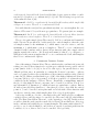
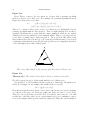
We emphasize that the attaching map must be defined on all of σ.
˙ That is, the
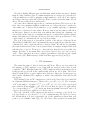
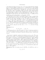
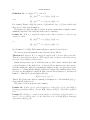
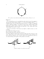
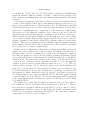
entire boundary of σ must be “glued” to X. For example, if X is a circle, then
Figure 1.1(i) shows one possible result of attaching a 1-cell to X. Attaching a 1-cell
to X cannot lead to the space illustrated in Figure 1.1(ii) since the entire boundary
of the 1-cell has not been “glued”to X.
(i)
(ii)
(i). A 1-cell attached to a circle. (ii). This is not a 1-cell attached to a circle
Figure 1.1.
We are now ready for our main definition. A finite CW complex is any topological
space X such that there exists a finite nested sequence
(1.1)
∅ ⊂ X0 ⊂ X1 ⊂ · · · ⊂ Xn = X
such that for each i = 0, 1, 2, . . . , n, Xi is the result of attaching a cell to X(i−1) .
Note that this definition requires that X0 be a 0-cell. If X is a CW complex, we
refer to any sequence of spaces as in (1.1) as a CW decomposition of X. Suppose that
in the CW decomposition (1.1), of the n + 1 cells that are attached, exactly cd are
d-cells. Then we say that the CW complex X has a CW decomposition consisting of
cd d-cells for every d.
We note that a (closed) d-simplex is a d-cell. Thus a finite simplicial complex is a
CW complex, and has a CW decomposition in which the cells are precisely the closed
simplices.
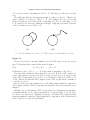
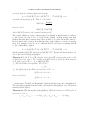
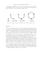
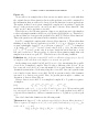
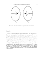
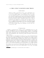
In Figure 1.2 we demonstrate a CW decomposition of a 2-dimensional torus which,
beginning with the 0-cell, requires attaching two 1-cells and then one 2-cell. Here
we can see one of the most compelling reasons for considering CW complexes rather
than just simplicial complexes. Every simplicial decomposition of the 2-torus has at
least 7 vertices, 21 edges and 14 triangles.
4
ROBIN FORMAN
X0
X1
X2
X3
A CW decomposition of a 2-torus
Figure 1.2.
It may seem that quite a bit has been lost in the transition from simplicial complexes
to general CW complexes. After all, a simplicial complex is completely described by
a finite amount of combinatorial data. On the other hand, the construction of a CW
decomposition requires the choice of a number of continuous maps. However, if one
is only concerned with the homotopy type of the resulting CW complex, then things
begin to look a bit more manageable. Namely, the homotopy type of X ∪f σ depends
only on the homotopy type of X and the homotopy class of f .
Theorem 1.3. Let h : X → X 0 denote a homotopy equivalence, σ a cell, and f1 :
σ˙ → X, f2 : σ˙ → X 0 two continuous maps. If h ◦ f1 is homotopic to f2 , then X ∪f1 σ
and X 0 ∪f2 σ are homotopy equivalent.
An important special case is when h is the identity map. We state this case separately
for future reference.
Corollary 1.4. Let X be a topological space, σ a cell, and f1 , f2 : σ˙ → X two
continuous maps. If f1 and f2 are homotopic, then X ∪f1 σ and X ∪f2 σ are homotopy
equivalent.
(See Theorem 2.3 on page 120 of [28].) Therefore, the homotopy type of a CW complex
is determined by the homotopy classes of the attaching maps. Since homotopy classes
are discrete objects, we have now recaptured a bit of the combinatorial atmosphere
that we seemingly lost when generalizing from simplicial complexes to CW complexes.
Let us now present some examples.
1) Suppose X is a topological space which has a CW decomposition consisting of
exactly one 0-cell and one d-cell. Then X has a CW decomposition ∅ ⊂ X0 ⊂ X1 = X.
The space X0 must be the 0-cell, and X = X1 is the result of attaching the d-cell
to X0 . Since X0 consists of a single point, the only possible attaching map is the
constant map. Thus X is constructed from taking a closed d-ball and identifying all
of the points on its boundary. One can easily see that this implies that the resulting
space is a d-sphere.
2) Suppose X is a topological space which has a CW decomposition consisting of
exactly one 0-cell and n d-cells. Then X has a CW decomposition as in (1.1) such that
A USER’S GUIDE TO DISCRETE MORSE THEORY
5
X0 is the 0-cell, and for each i = 1, 2, . . . , n the space Xi is the result of attaching a dcell to X(i−1) . From the previous example, we know that X1 is a d-sphere. The space
X2 is constructed by attaching a d-cell to X1 . The attaching map is a continuous map
from a (d − 1)-sphere to X1 . Every map of the (d − 1)-sphere into X1 is homotopic to
a constant map (since π(d−1) (X1 ) ∼
= π(d−1) (S d ) ∼
= 0). If the attaching map is actually
a constant map, then it is easy to see that the space X2 is the wedge of two d-spheres,
denoted by S d ∧ S d . (The wedge of a collection of topological spaces is the space
resulting from choosing a point in each space, taking the disjoint union of the spaces,
and identifying all of the chosen points.) Since the attaching map must be homotopic
to a constant map, Corollary 1.4 implies that X2 is homotopy equivalent to a wedge
of two d-spheres.
When constructing X3 by attaching a d-cell to X2 , the relevant information is a
map from S d−1 to X2 , and the homotopy type of the resulting space is determined
by the homotopy class of this map. All such maps are homotopic to a constant map
(since πd−1 (X2 ) ∼
= πd−1 (S d ∧ S d ) ∼
= 0). Since X2 is homotopy equivalent to a wedge
of two d-spheres, and the attaching map is homotopic to a constant map, it follows
from Theorem 1.3 that X3 is homotopy equivalent to the space that would result from
attaching a d-cell to S d ∧ S d via a constant map, i.e., X3 is homotopy equivalent to
a wedge of three d-spheres.
Continuing in this fashion, we can see that X must be homotopy equivalent to a
wedge of n d-spheres.
The reader should not get the impression that the homotopy type of a CW complex
is determined by the number of cells of each dimension. This is true only for very
few spaces (and the reader might enjoy coming up with some other examples). The
fact that wedges of spheres can, in fact, be identified by this numerical data partly
explains why the main theorem of many papers in combinatorial topology is that a
certain simplicial complex is homotopy equivalent to a wedge of spheres. Namely
such complexes are the easiest to recognize. However, that does not explain why so
many simplicial complexes that arise in combinatorics are homotopy equivalent to a
wedge of spheres. I have often wondered if perhaps there is some deeper explanation
for this.
3) Suppose that X is a CW complex which has a CW decomposition consisting
of exactly one 0-cell, one 1-cell and one 2-cell. Let us consider a CW decomposition
for X with these cells: ∅ ⊂ X0 ⊂ X1 ⊂ X2 = X. We know that X0 is the 0-cell.
Suppose that X1 is the result of attaching the 1-cell to X0 . Then X1 must be a circle,
and X2 arises from attaching a 2-cell to X1 . The attaching map is a map from the
boundary of the 2-cell, i.e., a circle, to X1 which is also a circle. Up to homotopy, such
a map is determined by its winding number, which can be taken to be a nonnegative
integer. If the winding number is 0, then without altering the homotopy type of
X we may assume that the attaching map is a constant map, which yields that
X ∼ S 1 ∧ S 2 (where ∼ denotes homotopy equivalence). If the winding number is
6
ROBIN FORMAN
1 then without altering the homotopy type of X we may assume that the attaching
map is a homeomorphism, in which case X is a 2-dimensional disc. If the winding
number is 2, then without altering the homotopy type of X we may assume that the
attaching map is a standard degree 2 mapping (i.e., that wraps one circle around
the other twice, with no backtracking). The reader should convince him/herself that
the result in this case is that X is the 2-dimensional projective space P2 . In fact,
each winding number results in a homotopically distinct space. These spaces can be
distinguished by their homology, since H1 (X, Z) for the space X resulting from an
attaching map with winding number n is isomorphic to Z/nZ.
It seems that we are not quite done with this example, because we assumed that
the 1-cell was attached before the 2-cell, and we must consider the alternative order,
in which X1 is the result of attaching a 2-cell to X0 . In this case, X1 is a 2-sphere,
and X = X2 is the result of attaching a 1-cell to X1 . The attaching map is a map
of S 0 into S 2 . Since S 2 is connected (i.e., π0 (S 2 ) = 0) all such maps are homotopic
to a constant map. Taking the attaching map to be a constant map yields that X =
S 1 ∧ S 2 . Thus adding the cells in this order merely resulted in fewer possibilities for
the homotopy type of X. This is a general phenomenon. Generalizing the argument
we just presented, using the fact that πi (S d ) = 0 for i < d, yields the following
statement.
Theorem 1.5. Let
(1.2)
∅ ⊂ X0 ⊂ X2 ⊂ · · · ⊂ Xn = X
be a CW decomposition of a finite CW complex X. Then X is homotopy equivalent to
a finite CW decomposition with precisely the same number of cells of each dimension
as in (1.2), and with the cells attached so that their dimensions form a nondecreasing
sequence.
I first learned of simplicial complexes in an algebraic topology course. They were
introduced as a category of topological spaces for which it was rather easy to define
homology and cohomology, i.e., in terms the simplicial chain- and cochain-complexes.
One might be concerned that in the transition from simplicial complexes to CW
complexes we have lost this ability to easily compute the homology. In fact, much of
this computability remains. Let X be a CW complex with a fixed CW decomposition.
Suppose that in this decomposition X is constructed from exactly cd cells of dimension
d for each d = 0, 1, 2, . . . , n = dim(K), and let Cd (X, Z) denote the space Zcd (more
precisely, Cd (X, Z) denotes the free abelian group generated by the d-cells of X, each
endowed with an orientation). The following is one of the fundamental results in the
theory of CW complexes.
Theorem 1.6. There are boundary maps ∂d : Cd (X, Z) → Cd−1 (X, Z), for each d, so
that
∂d−1 ◦ ∂d = 0
A USER’S GUIDE TO DISCRETE MORSE THEORY
7
and such that the resulting differential complex
∂
∂n−1
∂
n
1
0 −→ Cn (X, Z) −→
Cn−1 (X, Z) −→ · · · −→
C0 (X, Z) −→ 0
calculates the homology of X. That is, if we define
Ker(∂d )
Hd (C, ∂) =
Im(∂d+1 )
then for each d
Hd (C, ∂) ∼
= Hd (X, Z)
where Hd (X, Z) denotes the singular homology of X.
The actual definition of the boundary map ∂ is slightly nontrivial and we will not
go into it here (see Ch. V Sec. 2 of [28] for the details). At first it may seem that
without knowing this boundary map, there is little to be gained from Theorem 1.6.
In fact, much can be learned from just knowing of the existence of such a boundary
map. For example, let us choose a coefficient field F, and tensor everything with F
to get a differential complex
∂
∂n−1
∂
n
1
0 −→ Cn (X, F) −→
Cn−1 (X, F) −→ · · · −→
C0 (X, F) −→ 0
which calculates H∗ (X, F), where now Cd (X, F) ∼
= Fcd . From basic linear algebra. we
can deduce the following inequalities.
Theorem 1.7. Let X be a CW complex with a fixed CW decomposition with cd cells
of dimension d for each d. Fix a coefficient field F and let b∗ denote the Betti numbers
of X with respect to F, i.e., bd = dim(Hd (X, F)).
(i) (The Weak Morse Inequalities) For each d
cd ≥ bd .
(ii) Let χ(X) denote the Euler characteristic of X, i.e.,
χ(X) = b0 − b1 + b2 − . . . .
then we also have
χ(X) = c0 − c1 + c2 − . . . .
As the name “Weak Morse Inequalities” implies, this theorem can be strengthened.
The following inequalities, known as the “Strong Morse Inequalities” also follow from
standard linear algebra.
Theorem 1.8 (The Strong Morse Inequalities). With all notation as in Theorem 1.7,
for each d = 0, 1, 2, . . .
cd − cd−1 + cd−2 − · · · + (−1)d c0 ≥ bd − bd−1 + bd−2 − · · · + (−1)d b0 .
8
ROBIN FORMAN
Comparing Strong Morse Inequalities for consecutive values of d, and using the fact
that bi = 0 for i larger than the dimension of K, yields Theorem 1.7.
We mentioned earlier that a great benefit of passing from simplicial complexes to
the more general CW complexes is that one often can use many fewer cells. Let us
take another look at this phenomenon in light of the Morse inequalities. Consider the
case where X is a two-dimensional torus, so that with respect to any coefficient field
b0 = 1, b1 = 2, b2 = 1. From the weak Morse inequalities, we have that for any CW
decomposition,
c 0 ≥ b0 = 1
c 1 ≥ b1 = 2
c2 ≥ b2 = 1.
A simplicial decomposition is a special case of a CW decomposition, so these inequalities are satisfied when cd denotes the number of d-simplices in a fixed simplicial
decomposition. However, every simplicial decomposition has at least 7 0-simplices,
21 1-simplices and 14 2-simplices, so these inequalities are far from equality. It is
generally the case that for a simplicial decomposition these inequalities are very far
from optimal, and hence are generally of little interest. On the other hand, earlier
we demonstrated a CW decomposition of the two-torus with exactly one 0-cell, two
1-cells and one 2-cell. The inequalities tell us, in particular, that one cannot build a
two-torus using fewer cells.
2. The Basics of Discrete Morse Theory
The discussion in the previous section leads us to an important question. Suppose
one is given a finite simplicial complex X. Typically, we can expect that X has a CW
decomposition with many fewer cells than in the original simplicial decomposition.
How can one go about finding such an “efficient” CW decomposition for X? In this
section we present a technique, discrete Morse Theory, which can be useful in such
an investigation. (We note that the ideas we will describe can be applied with no
modification at all to any finite regular CW complex, and with only minor modifications to a general finite CW complex. However, for simplicity, in this paper we will
restrict attention to simplicial complexes.)
We begin by recalling that a finite simplicial complex is a finite set of vertices V ,
along with a set of subsets K of V . The set K satisfies two main properties:
1) V ⊆ K
2) If α ∈ K and β ⊆ α then β ∈ K.
By a slight abuse of notation, we will refer to the simplicial complex simply as K.
The elements of K are called simplices. If α ∈ K, and α contains p + 1 vertices,
then we say that the dimension of α is p, and we will sometimes denote this by α(p) .
For simplices α and β we will use the notation α < β or β > α to indicate that α
is a proper subset of β (thinking of α and β as subsets of V ), and say that α is a
A USER’S GUIDE TO DISCRETE MORSE THEORY
9
face of β. We emphasize that at this point we will not be placing any restrictions on
the finite simplicial complexes under investigation. In particular, the complexes need
not be manifolds (even though many of our examples will be). In Section 9 we will
briefly indicate how some of our conclusions can be strengthened in the case that the
complexes are assumed to have additional structure.
A discrete Morse function on K is a function which, roughly speaking, assigns
higher numbers to higher dimensional simplices, with at most one exception, locally,
at each simplex. More precisely,
Definition 2.1. A function
f : K −→ R
is a discrete Morse function if for every α(p) ∈ K
(1) #{β (p+1) > α | f (β) ≤ f (α)} ≤ 1,
and
(2) #{γ (p−1) < α | f (γ) ≥ f (α)} ≤ 1.
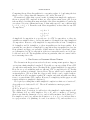
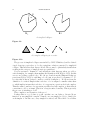
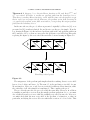
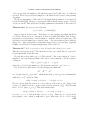
A simple example will serve to illustrate the definition. Consider the two complexes
shown in Figure 2.2. Here we indicate functions by writing next to each simplex the
value of the function on that simplex. The function (i) is not a discrete Morse function
as the edge f −1 (0) violates rule (2), since it has 2 lower dimensional “neighbors” on
which f takes on higher values, and the vertex f −1 (5) violates rule (1), since it has 2
higher dimensional “neighbors” on which f takes on lower values. The function (ii)
is a Morse function. Note that a discrete Morse function is not a continuous function
on K. Rather, it is an assignment of a single number to each simplex.
5
2
5
4
3
1
0
(i)
2
4
1
3
0
(ii)
(i). This is not a discrete Morse function. (ii). This is a discrete Morse function.
Figure 2.2.
The other main ingredient in Morse Theory is the notion of a critical point.
10
ROBIN FORMAN
Definition 2.3. A simplex α(p) is critical if
(1) #{β (p+1) > α | f (β) ≤ f (α)} = 0,
and
(2) #{γ (p−1) < α | f (γ) ≥ f (α)} = 0.
For example, Figure 2.2(ii), the vertex f −1 (0) and the edge f −1 (5) are critical, and
there are no other critical simplices.
We mention for later use that it follows from the axioms that a simplex cannot
simultaneously fail both conditions in the test for criticality.
Lemma 2.4. If K is a simplicial complex with a Morse function f , then for any
simplex α, either
(1) #{β (p+1) > α | f (β) ≤ f (α)} = 0,
or
(2) #{γ (p−1) < α | f (γ) ≥ f (α)} = 0.
(See Lemma 2.5 of [10].) This lemma will play a crucial role in Section 3.
We can now state the main theorem of discrete Morse Theory.
Theorem 2.5. Suppose K is a simplicial complex with a discrete Morse function.
Then K is homotopy equivalent to a CW complex with exactly one cell of dimension p
for each critical simplex of dimension p.
Rather than present a proof of this theorem, we will content ourselves here with
a brief discussion of the main ideas. A discrete Morse function gives us a way to
build the simplicial complex by attaching the simplices in the order prescribed by the
function, i.e., adding first the simplices which are assigned the smallest values. More
precisely, for any simplicial complex K with a discrete Morse function f , and any real
number c, define the level subcomplex K(c) by
K(c) = ∪f (α)≤c ∪β≤α β.
That is, K(c) is the subcomplex consisting of all simplices α of K such that f (α) ≤ c
along with all of their faces.
Theorem 2.5 follows from two basic lemmas.
Lemma 2.6. If there are no critical simplices α with f (α) ∈ (a, b], then K(b) is
homotopy equivalent to K(a). (In fact, K(b) collapses to K(a) — this will be explained
later.)
Lemma 2.7. If there is a single critical simplex α with f (α) ∈ (a, b] then there is a
map F : S (d−1) → K(a), where d is the dimension of α, such that K(b) is homotopy
equivalent to K(a) ∪F B d .
A USER’S GUIDE TO DISCRETE MORSE THEORY
11
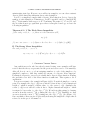
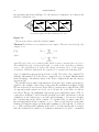
In Figure 2.8 we illustrate all of the level subcomplexes in the case that K is the
circle triangulated with 3 edges and 3 vertices, and f is the Morse function shown in
Figure 2.2 (ii). Here we can see why these lemmas are true.
5
2
2
1
0
K(0)
4
3
1
0
K(1)=K(2)
0
K(3)=K(4)
4
2
1
3
0
K(5)=K
The level subcomplexes of the discrete Morse function shown in Figure 2.2(ii)
Figure 2.8.
Let us begin with Lemma 2.6. Consider the transition from K(0) to K(1). We
have not added any critical simplices, and, just as the lemma predicts, K(0) and K(1)
are homotopy equivalent. Let us try to understand why the homotopy type did not
change. To construct K(1) from K(0), we first have to add the edge f −1 (1). This
edge is not critical because it has a codimension-one face which is assigned a higher
value, namely the vertex f −1 (2). In order to have K(1) be a subcomplex, we must
also add this vertex. Thus we see that the edge f −1 (1) in K(1) has a free face, i.e., a
face which is not the face of any other simplex in K(1). We can deformation retract
K(1) to K(0) by “pushing in” the edge f −1 (1) starting at the vertex f −1 (2).
This is a very general phenomenon. That is, it follows from the axioms for a discrete
Morse function that for any simplicial complex with any discrete Morse function, when
passing from one level subcomplex to the next the noncritical simplices are added in
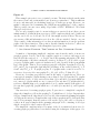
pairs, each of which consists of a simplex and a free face. Suppose that K2 ⊂ K1 are
simplicial complexes, and K1 has exactly two simplices α and β that are not in K2 ,
where β is a free face of α. Then it is easy to see that K2 is a deformation retract
of K1 , and hence K1 and K2 are homotopy equivalent (see Figure 2.9). This special
sort of combinatorial deformation retract is called a simplicial collapse. If one can
transform a simplicial complex K1 into a subcomplex K2 by simplicial collapses, then
we say that K1 collapses to K2 , and we indicate this by K1 & K2 . Figure 2.10 shows
a 2-dimensional simplex collapsing to one of its vertices.
12
ROBIN FORMAN
β
α
Κ2
Κ1
A simplicial collapse.
Figure 2.9.
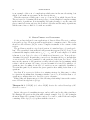
A 2-simplex collapsing to a vertex.
Figure 2.10.
The process of simplicial collapse was studied by J.H.C. Whitehead, and he defined
simple homotopy equivalence to be the equivalence relation generated by simplicial
collapse. This indicates that discrete Morse Theory may be particularly useful when
working in the category of simple homotopy equivalence.
Now let us turn to Lemma 2.7 and investigate what happens when one adds a
critical simplex, for example when making the transition from K(4) to K(5). In this
case we are adding a critical edge. We can see clearly from the illustration that we
pass from K(4) to K(5) by attaching a 1-cell, just as predicted by Lemma 2.7. To
see why this works in general, consider a critical d-simplex α. It follows from the
definition of a critical simplex that each face of α is assigned a smaller value than
α, which implies in turn that each face of α appears in a previous level subcomplex.
Thus the entire boundary of α appears in an earlier level subcomplex, so that when it
comes time to add α, we must “glue it in” along its entire boundary. This is precisely
the process of attaching a d-cell.
This completes our discussion of the proof.
Perhaps this is a good time to point out that one can define a discrete Morse
function on any simplicial complex. Namely, one can simply let f (α) = dim(α) for
each simplex α. In this case, every simplex is critical, and Theorem 2.5 is a rather
A USER’S GUIDE TO DISCRETE MORSE THEORY
13
uninteresting tautology. However, as we will see in examples, one can often construct
discrete Morse functions with many fewer critical simplices.
Let K be a simplicial complex with a discrete Morse function. Let mp denote the
number of critical simplices of dimension p. Let F be any field, and bp = dim Hp (K, F)
the pth Betti number with respect to F. Combining Theorems 2.5, 1.7 and 1.8, and
the fact that homotopy equivalent spaces have isomorphic homology, we have the
following inequalities.
Theorem 2.11. I. The Weak Morse Inequalities.
(i)For each p = 0, 1, 2, . . . , n (where n is the dimension of K)
m p ≥ bp .
(ii) m0 − m1 + m2 − · · · + (−1)n mn = b0 − b1 + b2 − · · · + (−1)n bn [= χ(K)].
II. The Strong Morse Inequalities.
For each p = 0, 1, 2, . . . , n, n + 1,
mp − mp−1 + · · · + (−1)p m0 ≥ bp − bp−1 + · · · + (−1)p b0 .
3. Gradient Vector Fields
Any ambitious reader who has already started trying some examples will have
noticed that the theory as presented in the previous section can be a bit unwieldy.
After all, how is one to go about assigning numbers to each of the simplices of a
simplicial complex so that they satisfy the axioms of a discrete Morse function?
Fortunately, in practice one need not actually find a discrete Morse function. Finding
the gradient vector field of the Morse function is sufficient. This requires a bit of
explanation.
Let us now return to the example in Figure 2.2(ii). Noncritical simplices occur in
pairs. For example, the edge f −1 (1) is not critical because it has a “lower dimensional
neighbor” which is assigned a higher value, i.e., the vertex f −1 (2). Similarly, the
vertex f −1 (2) is not critical because it has a “higher dimensional neighbor” which
is assigned a lower value, i.e., the edge f −1 (1). We indicate this pairing by drawing
an arrow from the vertex f −1 (2), pointing into the edge f −1 (1). Similarly, we draw
an arrow from the vertex f −1 (4) pointing into the edge f −1 (3). (See Figure 3.1.)
One can think of these arrows as pictorially indicating the simplicial collapse that is
referred to in the proof of Lemma 2.6.
14
ROBIN FORMAN
5
2
4
1
3
0
The gradient vector field of the Morse function shown in Figure 2.2 (ii).
Figure 3.1.
We can apply this process to any simplicial complex with a discrete Morse function.
The arrows are drawn as follows. Suppose α(p) is a non-critical simplex with β (p+1) > α
satisfying f (β) ≤ f (α). We then draw an arrow from α to β. Figure 3.2 illustrates
a more complicated example. Note that the discrete Morse function drawn in this
figure has one critical vertex, f −1 (0), and one critical edge, f −1 (11). Theorem 2.5
implies this simplicial complex is homotopy equivalent to a CW complex with exactly
one 0-cell and one 1-cell, i.e., a circle.
It follows from Lemma 2.4 that that every simplex α satisfies exactly one of the
following:
(i) α is the tail of exactly one arrow.
(ii) α is the head of exactly one arrow.
(iii) α is neither the head nor the tail of an arrow.
Note that a simplex is critical if and only if it is neither the tail nor the head of any
arrow. These arrows can be viewed as the discrete analogue of the gradient vector
field of the Morse function. (To be precise, when we say “gradient vector field” we
are really referring to the negative of the gradient vector field.)
6
7
10
9
8
14
16 17
5
12 13
3
11
4
(i)
15
0
1 2
(ii)
Another example of a gradient vector field
A USER’S GUIDE TO DISCRETE MORSE THEORY
15
Figure 3.2.
As we will see in examples later, these arrows are much easier to work with than
the original discrete Morse function. In fact, this gradient vector field contains all of
the information that we will need to know about the function for most applications.
The upshot is that if one is given a simplicial complex and one wishes to apply the
theory of the previous section, one need not find a discrete Morse function. One
“only” needs to find a gradient vector field.
This leads us to the following question. Suppose we attach arrows to the simplices
so that each simplex satisfies exactly one of properties (i),(ii),(iii) above. Then how do
we know if that set of arrows is the gradient vector field of a discrete Morse function?
This is the question we will answer in the remainder of this section.
Let K be a simplicial complex with a discrete Morse function f . Then rather than
thinking about the discrete gradient vector field V of f as a collection of arrows,
we may equivalently describe V as a collection of pairs {α(p) < β (p+1) } of simplices
of K, where {α(p) < β (p+1) } is in V if and only if f (β) ≤ f (α). In other words,
{α(p) < β (p+1) } is in V if and only if we have drawn an arrow that has α as its
tail, and β as its head. The properties of a discrete Morse function imply that each
simplex is in at most one pair of V . This leads us to the following definition.
Definition 3.3. A discrete vector field V on K is a collection of pairs {α(p) < β (p+1) }
of simplices of K such that each simplex is in at most one pair of V .
Such pairings were studied in [41] and [8] as a tool for investigating the possible
f -vectors for a simplicial complex. Here we take a different point of view. If one
has a smooth vector field on a smooth manifold, it is quite natural to study the
dynamical system induced by flowing along the vector field. One can begin the same
sort of study for any discrete vector field. In [12] we present a study of the dynamics
associated to a discrete vector field. Here, we present just enough to continue our
discussion of discrete Morse Theory.
Given a discrete vector field V on a simplicial complex K, a V −path is a sequence
of simplices
(3.1)
(p)
(p+1)
α0 , β0
(p)
(p+1)
, α1 , β1
(p)
(p)
, α2 , . . . , βr(p+1) , αr+1
such that for each i = 0, . . . r, {α < β} ∈ V and βi > αi+1 6= αi . We say such a path
is a non-trivial closed path if r ≥ 0 and α0 = αr+1 . If V is the gradient vector field of
a discrete Morse function f , then we sometimes refer to a V -path as a gradient path
of f .
One idea behind this definition is the following result.
Theorem 3.4. Suppose V is the gradient vector field of a discrete Morse function f .
Then a sequence of simplices as in (3.1) is a V -path if and only if αi < βi > αi+1 for
each i = 0, 1, . . . , r, and
f (α0 ) ≥ f (β0 ) > f (α1 ) ≥ f (β1 ) > · · · ≥ f (βr ) > f (αr+1 ).
16
ROBIN FORMAN
That is, the gradient paths of f are precisely those “continuous” sequences of simplices
along which f is decreasing. In particular, this theorem implies that if V is a gradient
vector field, then there are no nontrivial closed V -paths. In fact, the main result of
this section is that the converse is true.
Theorem 3.5. A discrete vector field V is the gradient vector field of a discrete
Morse function if and only if there are no non-trivial closed V -paths.
We will not prove this theorem here. However, many readers may notice the similarity with the following standard theorem from the subject of directed graphs.
Theorem 3.6. Let G be a directed graph. Then there is a real-valued function of the
vertices that is strictly decreasing along each directed path if and only if there are no
directed loops.
We will show in Section 6 that, in fact, Theorem 3.6 implies Theorem 3.5. The
power of Theorem 3.5 is indicated in the next two sections in which we construct some
discrete vector fields and use Theorem 3.5 to verify that they are gradient vector fields.
4. Our First Example: The Real Projective Plane
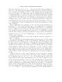
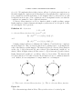
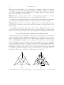
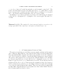
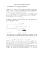
Figure 4.1 (i) shows a triangulation of the real projective plane P2 . Note that the
vertices along the boundary with the same labels are to be identified, as are the edges
whose endpoints have the same labels. In Figure 5(ii) we illustrate a discrete vector
field V on this simplicial complex. One can easily see that there are no closed V -paths
(since all V -paths go to the boundary of the figure and there are no closed V -paths
on the boundary), and hence is a gradient vector field. The only simplices which are
neither the head nor the tail of an arrow are the vertex labelled 1, the edge e, and
the triangle t. Thus, by Theorem 2.5, the projective plane is homotopy equivalent
to a CW complex with exactly one 0-cell, one 1-cell and one 2-cell. (Of course, we
already knew this from our discussion of Example 3 in Section 2.)
3
3
e
2
1
2
1
t
1
3
(i)
2
1
e
3
2
(ii)
(i) A triangulation of the real projective plane. (ii) A discrete gradient vector field on P2 .
A USER’S GUIDE TO DISCRETE MORSE THEORY
17
Figure 4.1.
This example gives rise to two potential concerns. The first is that from the main
theorem we learn only a statement about “homotopy equivalence”. This is sufficient
if one is only interested in calculating homology or homotopy groups. However, one
might be interested in determining the (PL-)homeomorphism type of the complex.
This is possible, in some cases, using deep results of J.H.C. Whitehead. We revisit
this topic in Section 8.
The second potential point of concern is that as we saw in Section 2 there are an
infinite number of different homotopy types of CW complexes which can be built from
exactly one 0-cell, one 1-cell and one 2-cell. One might wonder if Morse Theory can
give us any additional information as to how the cells are attached. In fact, one can
deduce much of this information if one has enough information about the gradient
paths of the Morse function. This point is discussed further in Section 7, where we
will return to this example of the triangulated projective plane.
5. Our Second Example: The Complex of Not Connected Graphs
A number of fascinating simplicial complexes arise from the study of monotone
graph properties. Let Kn denote the complete graph on n vertices, and suppose we
have labelled the vertices 1,2,. . . ,n. Let Gn denote the spanning subgraphs of Kn , that
is, the subgraphs of Kn that contain all n vertices. A subset P ⊂ Gn is called a graph
property of graphs with n vertices if inclusion in P only depends on the isomorphism
type of the graph. That is, P is a graph property if for all pairs of graphs G1 , G2 ∈ Gn ,
if G1 and G2 are isomorphic (ignoring the labellings on the vertices) then G1 ∈ P
if and only if G2 ∈ P. A graph property P of graphs with n vertices is said to be
monotone decreasing if for any graphs G1 ⊂ G2 ∈ Gn , if G2 ∈ P then G1 ∈ P.
Monotone decreasing properties abound in the study of graph theory. Here are
some typical examples: graphs having no more than k edges (for any fixed k), graphs
such that the degree of every vertex is less that δ (for any fixed δ), graphs which are
not connected, graphs which are not i-connected (for any fixed i), graphs which do
not have a Hamiltonian cycle, graphs which do not contain a minor isomorphic to H
(for any fixed graph H), graphs which are r-colorable (for any fixed r), and bipartite
graphs.
Any monotone decreasing graph property P gives rise to a simplicial complex K
where the d-simplices of K are the graphs G ∈ P which have d+1 edges. In particular,
if G is a d-simplex in K, then the faces of G are all of the nontrivial spanning subgraphs
of G (the monotonicity of P implies that each of these graphs is in K). Said in another
way, if P is nonempty, then the vertices of K are the edges of Kn , and a collection of
vertices in K span a simplex if the spanning subgraph of Kn consisting of all edges
which correspond to these vertices lies in P.
The simplicial complexes induced by many of the above-mentioned monotone decreasing graph properties have been studied using the techniques of this paper. See
18
ROBIN FORMAN
for example [6], [7], [21], [22], [27], [37]. These papers contain some beautiful mathematics in which the authors construct, “by hand”, explicit discrete gradient vector
fields, along the way illuminating some of the intricate finer structures of the graph
properties.
Some monotone graph properties have recently been the focus of intense interest
because of their relation to knot theory. Unfortunately this is probably not a good
time for an in depth discussion of this fascinating topic. We will mention only that
Vassiliev has shown how one can derive “finite type knot invariants” from the study
of the space of “singular knots” (i.e., maps from S 1 to R3 which are not embeddings).
The homology of the simplicial complexes of not connected and not 2-connected
graphs show up in his spectral sequence calculation of the homology of this space.
This is explained in [43], where Vassiliev derives the homotopy type of the complex
of not connected graphs. In [42] and [1], the topology of the space of not 2-connected
graphs is determined, with discrete Morse Theory playing a minor role in the latter
reference. This topic is reexamined in [37], in which the entire investigation is framed
in the language of discrete Morse Theory. Discrete Morse Theory is used to determine
the topology of not 3-connected graphs in [21].
In this section, we will provide an introduction to this work by taking a look at the
simpler case of the complex of not connected graphs. We will show how the ideas of
this paper may be used to determine the topology of Nn , the simplicial complex of
not connected graphs on n vertices. Let me begin by pointing out that this complex
can be well studied by more classical methods, and the answer has also been found by
Vassiliev in [43]. The only novelty of this section is our use of discrete Morse Theory.
Our goal is to construct a discrete gradient vector field V on Nn , the simplicial
complex of all not-connected graphs with the vertex set {1, 2, 3, . . . , n}. The construction will be in steps. Let V12 denote the discrete vector field consisting of all
pairs {G, G + (1, 2)}, where G is any graph in Nn which does not contain the edge
(1, 2) and such that G + (1, 2) ∈ Nn . Another way of describing V12 is that if G is
any graph in Nn which contains the edge (1, 2), then G − (1, 2) and G are paired in
V12 . Actually, there is one exception to this rule. Let G∗ denote the graph consisting
of only the single edge (1,2). Then G∗ − (1, 2) is the empty graph, which corresponds
to the empty simplex in Nn , and may not be paired in a discrete vector field. Thus,
G∗ is unpaired in V12 .
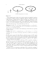
The graphs in Nn other than G∗ which are unpaired in V12 are those that do
not contain the edge (1, 2) and have the property that G + (1, 2) 6∈ Nn . That is,
those disconnected graphs G with the property that G + (1, 2) is connected. Such a
graph must have exactly two connected components, one of which contains the vertex
labelled 1, and one which contains the vertex labelled 2. We denote these connected
components by G1 and G2 , resp. See Figure 5.1.
A USER’S GUIDE TO DISCRETE MORSE THEORY
a
connected
graph
1
G1
2
19
a
connected
graph
G2
The graphs other than G∗ which are unpaired in the vector field V12 .
Figure 5.1.
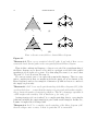
Let G be a graph other than G∗ which is unpaired in V12 , and consider vertex 3.
This vertex must either be in G1 or G2 . Suppose that vertex 3 is in G1 . If G does
not contain the edge (1, 3) then G + (1, 3) is also unpaired in V12 , so we can pair G
with G + (1, 3). If vertex 3 is in G1 , then the graph G is still unpaired if and only if
G contains the edge (1,3) and G − (1, 3) is the union of three connected components,
one containing vertex 1, one containing vertex 2, and one containing vertex 3.
Similarly, if vertex 3 is in G2 and G does not contain the edge (2, 3), then pair G
with G + (2, 3). Let V3 denote the resulting discrete vector field.
The unpaired graphs in V3 are G∗ and those that either contain the edge (1,3) and
have the property that G − (1, 3) is the union of three connected components, one
containing vertex 1, one containing vertex 2, and one containing vertex 3, or contain
the edge (2,3) and have the property that G − (2, 3) is the union of three connected
components, one containing vertex 1, one containing vertex 2, and one containing
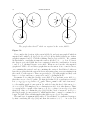
vertex 3. We illustrate these graphs in Figure 5.2. The circles in this figure indicate
connected graphs.
20
ROBIN FORMAN
1
3
2
1
2
3
The graphs other than G∗ which are unpaired in the vector field V3 .
Figure 5.2.
Now consider the location of the vertex labelled 4, and pair any graph G which is
unpaired in V3 with G + (1, 4), G + (2, 4), or G + (3, 4) if possible (at most one of these
graphs is unpaired in V3 ). Call the resulting discrete vector field V4 . We continue
in this fashion, considering in turn the vertices labelled 5, 6, . . . , n. Let Vi denote
the discrete vector field that has been constructed after the consideration of vertex
i, and V = Vn the final discrete vector field. When we are done the only unpaired
graphs in V will be G∗ and those graphs that are the union of two connected trees,
one containing the vertex 1 and one containing the vertex 2. In addition, both trees
have the property that the vertex labels are increasing along every ray starting from
the vertex 1 or the vertex 2. There are precisely (n − 1)! such graphs, and they each
have n − 2 edges, and hence correspond to an (n − 3)-simplex in Nn .
It remains to see that the discrete vector field V is a gradient vector field, i.e.,
that there are no closed V -paths. We first check that V12 is a gradient vector field.
(p)
(p+1)
(p)
Let γ = α0 , β0
, α1 denote a V12 -path. Then α0 must be the “tail of an arrow”,
i.e., the smaller graph of some pair in V12 , with β0 being the head of the arrow, i.e.,
β0 = α0 + (1, 2). The simplex α1 is a codimension-one face of β0 other than α0 . Thus,
α1 corresponds to a graph of the form α0 + (1, 2) − e, where e is an edge of α0 other
than (1,2). Since α1 contains the edge (1, 2) it is the “head of an arrow” in V12 , i.e.,
the larger graph of some pair in V12 , which implies that γ cannot be continued to a
longer V12 -path. This certainly implies that there are no closed V12 -paths.
The same sort of argument will work for V . Recall that V is constructed in stages,
by first considering the edge (1,2) and then the vertices 3, 4, 5, . . . in order. Let
A USER’S GUIDE TO DISCRETE MORSE THEORY
21
γ = α0 , β0 , α1 denote a V -path. In particular, α0 and β0 must be paired in V . The
reader can check that if α0 and β0 are first paired in Vi , i ≥ 3, then either α1 is the
head of an arrow in Vi , in which case the V -path cannot be continued, or α1 is paired
in Vi−1 . It follows by induction that there can be no closed V -paths.
In summary, V is a discrete gradient vector field on Nn with exactly one unpaired
vertex, and (n − 1)! unpaired (n − 3)-simplices. We can now apply Theorem 2.5 to
conclude
Theorem 5.3 ([43]). The complex Nn of not connected graphs on n-vertices is homotopy equivalent to the wedge of (n − 1)! spheres of dimension (n − 3).
6. A Combinatorial Point of View
The notion of a gradient vector field has a very nice purely combinatorial description
due to Chari [6], using which we can recast the Morse Theory in an appealing form.
We begin with the Hasse diagram of K, that is, the partially ordered set of simplices
of K ordered by the face relation. Consider the Hasse diagram as a directed graph.
The vertices of the graph are in 1-1 correspondence with the simplices of K, and there
is a directed edge from β to α if and only if α is a codimension-one face of β. (See
Figure 6.1 (i).) Now let V be a combinatorial vector field. We modify the directed
graph as follows. If {α < β} ∈ V then reverse the orientation of the edge between α
and β, so that it now goes from α to β. (See Figure 6.1(ii).) A V -path can be thought
of as a directed path in this modified graph. There are some directed paths in this
modified Hasse diagram which are not V -paths as we have defined them. However,
the following result is not hard to check.
22
ROBIN FORMAN
t
v1
e3
v3
t
e1
e2
v
2
e1
e2
e3
v1
v2
v3
(i)
v1
e3
v3
t
e2
t
e1
v2
e1
e2
e3
v1
v2
v3
(ii)
From a discrete vector field to a directed Hasse diagram.
Figure 6.1.
Theorem 6.2. There are no nontrivial closed V -paths if and only if there are no
nontrivial closed directed paths in the corresponding directed Hasse diagram.
Thus, in this combinatorial language, a discrete vector field is a partial matching of
the Hasse diagram, and a discrete vector field is a gradient vector field if the partial
matching is acyclic in the above sense. Note that using Theorem 6.2, we can see that
Theorem 3.5 does follow from Theorem 3.6.
We can now restate some of our earlier theorems in this language. There is a very
minor complication in that one usually includes the empty set as an element of the
Hasse diagram (considered as a simplex of dimension -1) while we have not considered
the empty set previously.
Theorem 6.3. Let V be an acyclic partial matching of the Hasse diagram of K (of the
sort described above — assume that the empty set is not paired with another simplex).
Let up denote the number of unpaired p-simplices. Then K is homotopy equivalent to
a CW-complex with exactly up cells of dimension p, for each p ≥ 0.
An important special case is when V is a complete matching, that is, every simplex
(this time including the empty simplex) is paired with another simplex. In this case,
Lemma 2.9 implies the following result.
Theorem 6.4. Let V be a complete acyclic matching of the Hasse diagram of K,
then K collapses onto a vertex, so that, in particular, K is contractible.
A USER’S GUIDE TO DISCRETE MORSE THEORY
23
This result was used in a very interesting fashion in [1].
7. The Morse Complex
In this section we will see how knowledge of the gradient paths of a discrete Morse
function on a space K can allow one to strengthen the conclusions of the main theorems. In particular, rather than just knowing the number of cells in a CW decomposition for K, one can calculate the homology exactly.
Let K be a simplicial complex with a Morse function f . Let Cp (X, Z) denote the
space of p-simplicial chains, and Mp ⊆ Cp (X, Z) the span of the critical p-simplices.
We refer to M∗ as the space of Morse chains. If we let mp denote the number of
critical p-simplices, then we obviously have
Mp ∼
= Zmp .
Since homotopy equivalent spaces have isomorphic homology, the following theorem
follows from Theorems 2.5 and 1.6.
Theorem 7.1. There are boundary maps ∂˜d : Mp → Md−1 , for each d, so that
∂˜d−1 ◦ ∂˜d = 0
and such that the resulting differential complex
(7.1)
∂˜n−1
∂˜
∂˜
n
1
0 −→ Mn −→
Mn−1 −→ · · · −→
M0 −→ 0
calculates the homology of X. That is, if we define
˜
˜ = Ker(∂d )
Hd (M, ∂)
Im(∂˜d+1 )
then for each d
˜ ∼
Hd (M, ∂)
= Hd (X, Z).
In fact, this statement is equivalent to the Strong Morse inequalities. The main
˜ This
goal of this section is to present an explicit formula for the boundary operator ∂.
requires a closer look at of the notion of a gradient path. Let α and α
˜ be p-simplices.
Recall from Section 7 that a gradient path from α
˜ to α is a sequence of simplices
(p)
(p+1)
α
˜ = α0 , β0
(p)
(p+1)
, α1 , β1
(p)
(p)
, α2 , . . . , βr(p+1) , αr+1 = α
such that αi < βi > αi+1 for each i = 0, 1, 2, . . . , r and f (α0 ) ≥ f (β0 ) > f (α1 ) ≥
f (β1 ) > · · · ≥ f (βr ) > f (αr+1 ). Equivalently, if V is the gradient vector field of f , we
require that for each i, αi and βi be paired in V and βi > αi+1 6= αi . In Figure 7.2 we
show a single gradient path from the boundary of a critical 2-simplex β to a critical
edge α, where the arrows indicate the gradient vector field V .
Given a gradient path as shown in Figure 7.2, an orientation on β induces an
orientation on α. We will not state the precise definition here. The idea is that
one “slides” the orientation from β along the gradient path to α. For example, for
24
ROBIN FORMAN
the gradient path shown in Figure 7.2, the indicated orientation on β induces the
indicated orientation on α.
α
β
A gradient path from the boundary of β to α.
Figure 7.2.
We are now ready to state the desired formula.
Theorem 7.3. Choose an orientation for each simplex. Then for any critical (p + 1)simplex β set
X
e =
(7.2)
∂β
cα,β α
critical α(p)
where
cα,β =
X
m(γ)
γ∈Γ(β,α)
where Γ(β, α) is the set of gradient paths which go from a maximal face of β to α.
The multiplicity m(γ) of any gradient path γ is equal to ±1, depending on whether,
given γ, the orientation on β induces the chosen orientation on α, or the opposite
orientation. With this differential, the complex (7.1) computes the homology of K.
A proof of this theorem appears in Section 8 of [10]. We refer to the complex (7.1)
with the differential (7.2) as the Morse complex (it goes by many different names
in the literature). An extensive study of the Morse complex in the smooth category
appears in [36].
We end this section with a demonstration of how the ideas of this section may be
applied to the example of the real projective plane P2 as illustrated in Figure 4.1(ii).
We saw in Section 2 how discrete Morse Theory can help us see that P2 has a CW
decomposition with exactly one 0-cell, one 1-cell and one 2-cell. Here we will see
how Morse Theory can distinguish between the spaces which have such a CW decomposition. In Figure 7.4 we redraw the gradient vector field, and indicate a chosen
orientation on the critical edge e and the critical triangle t. Let us now calculate
˜
the boundary map in the Morse complex. To calculate ∂(e),
we must count all of
the gradient paths from the boundary of e to v. There are precisely two such paths.
Namely, following the unique gradient path beginning at each endpoint of e leads us
to v. (The gradient path beginning at the head of e is the trivial path of 0 steps.)
Since the orientation of e induces a + orientation on the head of e, and a − orientation
A USER’S GUIDE TO DISCRETE MORSE THEORY
25
on the tail of e, adding these two paths with their corresponding signs leads us to the
˜ = 0. It can be seen from the illustration that there are precisely two
formula that ∂(e)
gradient paths from the boundary of t to e, and, with the illustrated orientation for t,
˜ = 2e. Therefore the homology
both induce the chosen orientation on e, so that ∂(t)
of the real projective plane can be calculated from the following differential complex.
×2
0
Z −→ Z −→ Z −→ 0.
Thus we see that
H0 (P2 , Z) ∼
= Z, H1 (P2 , Z) ∼
= Z/2Z, H2 (P2 , Z) ∼
= 0.
3
e
2
1
t
1
e
3
2
A gradient vector field on the real projective plane.
Figure 7.4.
8. Sphere Theorems
As mentioned in our discussion at the end of Section 4, one can sometimes use
discrete Morse Theory to make statements about more than just the homotopy type
of the simplicial complex. One can sometimes classify the complex up to homeomorphism or combinatorial equivalence. This will be a very short section, as this topic
seems a bit far from the main thrust of this paper. In addition, some terms will unfortunately have to be defined only cursorily or not at all. So far, we have not placed
any restrictions on the simplicial complexes under consideration. The main idea of
this section is that if our simplicial complex has some additional structure, then one
may be able to strengthen the conclusion. This idea rests on some very deep work of
J.H.C. Whitehead [44].
Recall that a simplicial complex K is a combinatorial d-ball if K and the standard
d-simplex Σd have isomorphic subdivisions. A simplicial complex K is a combinatorial (d − 1)-sphere, if K and Σ˙d have isomorphic subdivisions (where Σ˙d denotes the
boundary of Σd with its induced simplicial structure). A simplicial complex K is a
26
ROBIN FORMAN
combinatorial d-manifold with boundary if the link of every vertex is either a combinatorial (d − 1)-sphere or a combinatorial (d − 1)-ball. The following is a special case
of the main theorem of [44].
Theorem 8.1. Let K be a combinatorial d-manifold with boundary which simplicially
collapses to a vertex. Then K is a combinatorial d-ball.
It is with this theorem (and its generalizations) that one can strengthen the conclusion of Theorem 2.5 beyond homotopy equivalence. We present just one example.
Theorem 8.2. Let X be a combinatorial d-manifold with a discrete Morse function
with exactly two critical simplices. Then X is a combinatorial d-sphere.
The proof is quite simple (given Theorem 8.1). If X is a combinatorial d-manifold
with a discrete Morse function f with exactly two critical simplices, then the critical simplices must be the minimum of f , which must occur at a vertex v, and the
maximum of f , which must occur at a d-simplex α. Then X − α is a combinatorial
d-manifold with boundary with a discrete Morse function with only a single critical
simplex, namely the vertex v. It follows from Lemma 2.6 that X − α collapses to v.
Whitehead’s theorem now implies that X − α is a combinatorial d-ball, which implies
that X is a combinatorial d-sphere.
9. Cancelling Critical Points
One of the main problems in Morse Theory, whether in the combinatorial or smooth
setting, is to find a Morse function for a given space with the fewest possible critical
points (much of the book [38] is devoted to this topic). In general this is a very
difficult problem, since, in particular, it contains the Poincar´e conjecture — spheres
can be recognized as those spaces which have a Morse function with precisely 2 critical
points. In [31], Milnor presents Smale’s proof [40] of the higher dimensional Poincar´e
conjecture (in fact, a proof is presented of the more general h-cobordism theorem)
completely in the language of Morse Theory. Drastically oversimplifying matters,
the proof of the higher Poincar´e conjecture can be described as follows. Let M be a
smooth manifold of dimension ≥ 5 which is homotopy equivalent to a sphere. Endow
M with a (smooth) Morse function f . One then proceeds to show that the critical
points of f can be cancelled out in pairs until one is left with a Morse function with
exactly two critical points, which implies that M is a (topological) sphere.
A key step in this proof is the “cancellation theorem” which provides a sufficient
condition for two critical points to be cancelled (see Theorem 5.4 in [31], which Milnor
calls “The First Cancellation Theorem”, or the original proof in [33]). In this section
we will see that the analogous theorem holds for discrete Morse functions. Moreover,
in the combinatorial setting the proof is much simpler. The main result is that if α(p)
and β (p+1) are 2 critical simplices, and if there is exactly 1 gradient path from the
boundary of β to α, then α and β can be cancelled. More precisely,
A USER’S GUIDE TO DISCRETE MORSE THEORY
27
Theorem 9.1. Suppose f is a discrete Morse function on M such that β (p+1) and
α(p) are critical, and there is exactly one gradient path from the boundary β to α.
Then there is another Morse function g on M with the same critical simplices except
that α and β are no longer critical. Moreover, the gradient vector field associated to
g is equal to the gradient vector field associated to f except along the unique gradient
path from the boundary β to α.
In the smooth case, the proof, either as presented originally by Morse in [33] or as
presented in [31], is rather technical. In our discrete case the proof is simple. If, in the
top drawing in Figure 9.2, the indicated gradient path is the only gradient path from
the boundary of β to α, then we can reverse the gradient vector field along this path,
replacing the figure by the vector field shown in the bottom drawing in Figure 9.2.
α
β
Cancelling critical points.
Figure 9.2.
The uniqueness of the gradient path implies that the resulting discrete vector field
has no closed orbits, and hence, by Theorem 3.5, is the gradient vector field of some
Morse function. Moreover, α and β are not critical for this new Morse function, while
the criticality of all other simplices is unchanged. This completes the proof.
The proof in the smooth case proceeds along the same lines. However, in addition
to turning around those vectors along the unique gradient path from β to α, one must
also adjust all nearby vectors so that the resulting vector field is smooth. Moreover,
one must check that the new vector field is the gradient of a function, so that, in
particular, modifying the vectors did not result in the creation of a closed orbit. This
28
ROBIN FORMAN
is an example of the sort of complications which arise in the smooth setting, but
which do not make an appearance in the discrete theory.
This theorem was recently put to very good use in [2], in which discrete Morse
Theory is used to determine the homotopy type of some simplicial complexes arising
in the study of partitions. It is fascinating, and quite pleasing, to see the same idea
play a central role in two subjects, the Poincar´e conjecture and the study of partitions,
which seem to have so little to do with one another.
10. Morse Theory and Evasiveness
So far, we have indicated some applications of discrete Morse Theory to combinatorics and topology. We now present an application to computer science. The reader
should see the reference [14] for a more complete treatment of the content of this
section.
The problem we study is a topological version of a standard type of “search problem”. The generalized version that we will present first appeared in [35]. Let S be an
n-dimensional simplex, with vertices v0 , v1 , . . . , vn , and K a subcomplex of S which
is known to you. Let σ be a face of S which is not known to you. Your goal is to
determine if σ is in K. In particular, you need not determine the face σ, just whether
or not it is in K. You are permitted to ask questions of the form “Is vi in σ?”. You
may use the answers to the questions you have already asked in determining which
vertex to ask about next. Of course, you can determine if σ is in K by asking n + 1
questions, since by asking about all n + 1 vertices you can completely determine σ.
You win this game if you answer the given question after asking fewer than n + 1
questions.
Say that K is nonevasive if there is a winning strategy for this game, i.e there
is a question algorithm that determines whether or not σ ∈ K in fewer than n + 1
questions, no matter what σ is. Say K is evasive otherwise.
Kahn, Saks and Sturtevant proved the following relationship between the evasiveness of K and its algebraic topology.
˜ ∗ (K) 6= 0, where H
˜ ∗ (K) denotes the reduced homology of K,
Theorem 10.1. If H
then K is evasive.
In fact, they proved something stronger, and we will come back to this point later.
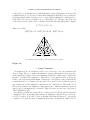
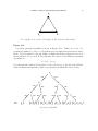
We illustrate the previous theorem with a simple example. Let S be the 2-simplex
shown in Figure 10.2, spanned by the vertices v0 , v1 and v2 , with K the subcomplex
consisting of the edge [v0 , v1 ] together with the vertex v2 .
A USER’S GUIDE TO DISCRETE MORSE THEORY
29
v2
v0
v1
An example of an evasive subcomplex of the 2-dimensional simplex.
Figure 10.2.
A possible guessing algorithm is shown in Figure 10.3. Define an evader of a
guessing algorithm to be a face σ of S with the property that when questions are asked
in the order determined by the algorithm one must ask all three questions before it is
known whether or not σ is in K. In particular, the evaders of the illustrated guessing
algorithm are:
σ = [v2 ], [v0 , v2 ]
Note that the subcomplex K has nonzero reduced homology, so the theorem of Kahn,
Saks and Sturtevant guarantees that every guessing algorithm has some evaders.
v2
no
yes
v0
no
v1
no
σ=
[]
yes no
v1
yes
no
v1
v0
yes
yes
v0
no
yes
no
yes
[v ] [v0 ] [v0 ,v ] [v2 ] [v ,v ] [v ,v ] [v ,v ,v ]
1
1
A guessing algorithm
0
2
1
2
0
1
2
30
ROBIN FORMAN
Figure 10.3.
Morse Theory comes to the fore when one observes that a guessing algorithm
induces a discrete vector field on S. For example, the guessing algorithm shown in
Figure 10.3 induces the vector field
V =
{ {∅ < [v1 ]}, {[v0 ] < [v0 , v1 ]},
{[v2 ] < [v0 , v2 ]}, {[v1 , v2 ] < [v0 , v1 , v2 ]} }
That is, V consists of those pairs of faces of S which are not distinguished by the
guessing algorithm until the last question. There is slight subtlety here in that a
guessing algorithm pairs a vertex with the empty simplex ∅, while in our original
definition, it was not permitted to pair a simplex with ∅. Thus, to get a true discrete
vector field, we must remove this pair from V . (It is precisely this subtle point
that results in the reduced homology of K being the relevant measure of topological
complexity, rather than the nonreduced homology.) However, for simplicity, from now
on we will simply ignore this technical point.
v2
v0
v1
The vector field induced by the guessing algorithm shown in Figure 10.3.
Figure 10.4.
Theorem 10.5. This induced vector field is always a gradient vector field.
We will postpone the proof of this result until the end of this section.
Now restrict V to K (by taking only those pairs in V such that both simplices are
in K). For example, in our example, this results in the vector field
VK = {{[v0 ] < [v0 , v1 ]}}.
From the previous theorem, V has no closed orbits. Any discrete vector field consisting
of a subset of the pairs of V has fewer paths, and hence also has no closed orbits.
Therefore, VK is a gradient vector field on K. Note that V pairs every face of S with
another face, and hence there are no critical simplices (we are continuing to ignore
for now the simplex which is paired with the emptyset). Thus, the critical simplices
A USER’S GUIDE TO DISCRETE MORSE THEORY
31
of VK are precisely the simplices of K which are paired in V with a face of S which is
not in K. These are precisely the simplices of K which are the evaders of the guessing
algorithm.
The Morse inequalities of Theorem 2.11 (i) imply that the number of evaders in K
e ∗ (K). Evaders occur in pairs, with each pair having one face of K and
is at least dim H
one face not in K. This yields the following quantitative refinement of Theorem 10.1.
Theorem 10.6. For any guessing algorithm
e ∗ (K)
# of evaders ≥ 2 dim H
Suppose that K is nonevasive. Then there is some guessing algorithm which has
no evaders. From our above discussion we have seen that this implies that K has a
gradient vector field with no critical simplices. Actually, this is not quite true. The
gradient vector field must have a critical vertex — the vertex that is paired with the
empty set — this is that minor technicality that we have been ignoring. Applying
Lemma 2.6 yields the following strengthening of Theorem 10.1.
Theorem 10.7. If K is nonevasive, then K simplicially collapses to a point.
This theorem appears in [23]. The interested reader can consult [14] for some additional refinements of this theorem.
We end this section with a proof of Theorem 10.5. Fix a subcomplex K of an nsimplex S, and a guessing algorithm. Associate to each p-simplex α of S the sequence
of integers
n(α) = n0 (α) < n1 (α) < · · · < np (α)
where the ni (α)’s are the numbers of the questions answered “yes” if σ = α.
If V is the vector field induced by the guessing algorithm and
(p)
(p+1)
α0 , β0
(p)
, α1
is a V -path, then {α0 , β0 } is in V , which means that α0 and β0 are not distinguished
until the (n + 1)st question. Thus,
n(β0 ) = n0 (α0 ) < n1 (α0 ) < · · · < np (α0 ) < n + 1.
We now observe that the vertices of a1 are a subset of the vertices of b0 . Suppose the
vertex of β0 which is not in α1 is the vertex tested in question ni (β0 ). Then we must
have i 6= n + 1 (since α0 6= α1 ). This demonstrates that
n(α1 ) = n0 (α0 ) < n1 (α0 ) < · · · < ni−1 (α0 ) < ni (α1 ) < . . .
for some i < n + 1, and such that ni (α1 ) > ni (α0 ). Thus n(α1 ) > n(α0 ) in the
lexicographic order, which is sufficient to prove that there are no closed orbits.
QED
32
ROBIN FORMAN
11. Further Thoughts
We close this paper with some additional thoughts on the subjects discussed in this
paper.
I would like to begin by encouraging the reader to take a look at the papers [24],
[25], and [3]. In these papers, discrete Morse Theory is used to investigate quite
interesting problems. These references were not mentioned earlier only because they
did not easily fit into any of the previous sections of this paper.
There are a number of directions in which discrete Morse Theory can be extended
and generalized. Here we mention a few such possibilities. In [16] we show how one
can recover the ring structure of the cohomology of a simplicial complex from the
point of view of discrete Morse Theory (this follows work of Betz and Cohen [4] and
Fukaya [17, 18] in the smooth setting). In [34], Novikov presents a generalization
of standard smooth Morse Theory in which the role of the Morse function is now
played by a closed 1-form (the classical case arises when the closed 1-form is exact).
In [15] we present the analogous generalization for discrete Morse Theory. In [45],
Witten shows how smooth Morse Theory can be seen as arising from considerations
of supersymmetry in quantum physics. In [11] we present a combinatorial version of
Witten’s derivation. We believe that this latter work may have greater significance.
At crucial points in [45], Witten appeals to path integral arguments which are rather
standard in quantum physics, but are ill-defined mathematically. In the corresponding
moments in [11] what arises is a well-defined discrete sum. Perhaps the approach in
[11] can find uses in the analysis of other quantum field theories.
One topic which we have only touched upon is the study of the dynamics associated
to flowing along the gradient vector field associated to a discrete Morse function. In
fact, an understanding of the dynamics is crucial to the proof of theorem 7.3, for
example. The relevant study takes place in Section 6 of [10]. In [12] we study the
dynamical properties of the flow associated to a general discrete vector field.
One area in which much work remains to be done is the investigation of discrete
Morse Theory for infinite simplicial complexes. The theory as described in this paper
can be applied without change to an infinite simplicial complex K endowed with a
discrete Morse function f which is proper, i.e., one in which for each real number c
the level subcomplex K(c) is a finite complex. Unfortunately, properness is often an
unnatural requirement when considering the infinite simplicial complexes which arise
in practice. In the interesting paper [29], discrete Morse Theory is applied to the
investigation of infinite simplicial complexes K which arise as a covering space of a
finite simplicial complex K 0 . In this case, the authors restrict attention to discrete
Morse functions which are lifts of a Morse function on K 0 , and compare the number
of critical simplices to the L2 -Betti numbers of K. While it appears to be too much
to hope that one can develop a useful theory that applies to all infinite simplicial
complexes with no restrictions on the discrete Morse function, it seems likely that
A USER’S GUIDE TO DISCRETE MORSE THEORY
33
there is room for very useful investigations of large classes of complexes and functions
with restrictions different than those already considered.
I will close these notes with some comments of a less rigorous nature. Whether in
the smooth category or the combinatorial category, Morse Theory is not essential to
any problem, it is usually “only” a convenient and efficient language. Anything that
can be done with Morse Theory can be done without it. It seems to me that Morse
Theory takes on a special significance in three different cases. First are the cases in
which Morse Theory is not intrinsic to the problem, but where the existence of such
an efficient language may make the difference between whether or not one is able to
see the way to the end of a problem. The best example of this in the smooth setting, I
think, is the proof of the higher dimensional Poincar´e conjecture ([39], [31]). Most of
the applications of discrete Morse Theory mentioned in Section 5, for example, seem
to fall into this category. Second are the cases in which the space one is studying
comes naturally endowed with a Morse function, or a gradient vector field. Here the
prime example is Bott’s proof of Bott periodicity ([5], see also Part IV of [30]), resting
on the fact that the loop space of a Riemannian manifold is endowed with a natural
Morse function. In the combinatorial setting, I would place the Morse-theoretic examination of evasiveness of the previous section in this category. Third are the cases
in which the objects under investigation can be naturally identified as the critical
points of a Morse function on a larger space. Examples of this phenomenon abound
in differential geometry, where one often studies extremals of energy functionals. In
particular, Morse’s first great triumph with Morse Theory was his investigation of the
set of geodesics between two points in a Riemannian manifold ([32], see also Part III
of [30]). The geodesics are precisely the critical points of the natural Morse function
on the path space, and Morse used the Morse inequalities, along with a knowledge
of the topology of the path space, to deduce the existence of many critical points.
It is intriguing to this author that there are as yet no corresponding examples in
the combinatorial setting. I know of no examples in which a collection of classically
studied objects in combinatorics can be naturally identified with the critical simplices
of a Morse function on some larger complex. Indeed, I believe that soon combinatorial examples of interest will be found that fit into this third category. I wonder if
applications of discrete Morse theory will be found that approach the beauty, depth
and fundamental significance of the applications of smooth Morse Theory mentioned
in this paragraph.
On a broader note, I believe that discrete Morse Theory is only a small part of what
someday will be a more complete theory of “combinatorial differential topology”,
although I hesitate to predict (at least in print) what form such a theory will take.
34
ROBIN FORMAN
References
[1] E. Babson, A. Bj¨
orner, S. Linusson, J. Shareshian and V. Welker, Complexes of not iConnected Graphs, Topology 38 (1999), pp. 271-299.
[2] E. Babson, P. Hersh, Discrete Morse functions from lexicographic orders, to appear in
Topology.
[3] E. Batzies and V. Welker Discrete Morse Theory for Cellular Resolutions, J. Reine Angew.
Math. 543 (2002), pp. 147–168.
[4] M. Betz and R. Cohen, Graph moduli space and cohomology operations, Turk. J. of Math.
18 (1994), pp. 23-41.
[5] R. Bott, Stable homotopy of the classical groups, Ann. of Math. 70 (1959), pp. 313-337.
[6] M. Chari, On Discrete Morse Functions and Combinatorial Decompositions, Discrete
Math. 217 (2000), pp. 101-113.
[7] X. Dong, The Topology of Bounded Degree Graph Complexes and Finite Free Resolutions,
thesis, Univ. of Minn., 2001.
[8] A. Duval A Combinatorial Decomposition of Simplicial Complexes, Israel J. of Math. 87
(1994), pp. 77-87.
[9] R. Forman, A Discrete Morse Theory for Cell Complexes, in: Geometry, Topology &
Physics for Raoul Bott, S.T. Yau (ed.), International Press, 1995.
, Morse Theory for Cell Complexes, Adv. in Math. 134 (1998), pp. 90-145.
[10]
[11]
, Witten-Morse Theory for Cell Complexes, Topology 37 (1998), pp. 945-979.
[12]
, Combinatorial Vector Fields and Dynamical Systems, Math. Zeit. 228 (1998),
pp. 629-681.
[13]
, Combinatorial differential topology and geometry, in: New Perspectives in Algebraic Combinatorics (Berkeley, CA. 1996-97), Math. Sci. Res. Inst. Publ. 38, Cambridge
Univ. Press, Cambridge, 91999), pp. 177-206.
[14]
, Morse Theory and Evasiveness, Combinatorica 20 (2000), pp. 498-504.
[15]
, Novikov-Morse theory for cell complexes, to appear in Int. J. of Math.
[16]
The Cohomology Ring and Discrete Morse Theory, preprint 2001.
[17] K. Fukaya, Morse homotopy, A∞ -category, and Floer homologies, in: Proc. Garc. Workshop on Geometry and Topology ’93, (Seoul, 1993), ed. H. J. Kim, Lecture Notes Ser. 18,
Seoul National University, pp 1-102.
[18]
, Morse homotopy and its quantization, in: Geometric Topology (Athens, GA
˙ Amer. Math. Soc., Prov. RI, 1997, pp. 409-440.
1993),AMS/IP Stud. Adv. Math21,
[19] M. Goresky and R. MacPherson Stratified Morse Theory, in: Singularities, Part I (Arcata,
CA, 1981), Proc. Sympos. Pure Math., 40, Amer. Math. Soc., R.I., (1983), pp. 517-533.
[20]
Stratified Morse Theory, Ergebnisse der Mathematik und ihrer Grenzgebiete (3),
14, Springer Verlag, Berlin-New York, 1988.
[21] J. Jonsson, On the homology of some complexes of graphs, preprint, 1998.
[22]
, The decision tree method, preprint, 1999.
[23] J. Kahn, M. Saks and D. Sturtevant A topological approach to evasiveness, Combinatorica
4 (1984), pp. 297-306.
[24] D. Kozlov, Collapsibility of ∆(Πn )/Sn and some related CW complexes, Proc. Amer.
Math. Soc. 128 (2000), pp. 2253-2259.
[25]
, Topology of spaces of hyperbolic polynomials with multiple roots, to appear in
Israel J. Math.
[26] W. K¨
uhnel, Triangulations of Manifolds with few Vertices, in: Advances in Differential
Geometry and Topology, World Sci. Publishing, N.J., (1990), pp. 59-114.
A USER’S GUIDE TO DISCRETE MORSE THEORY
35
[27] S. Linusson and J. Shareshian, Complexes of t-colorable graphs, preprint.
[28] A. Lundell and S. Weingram, The Topology of CW Complexes, Van Nostrand Reinhold
Company, New York, 1969.
[29] V. Mathai and S.G. Yates, Discrete Morse theory and extended L2 homology, J. Funct.
Anal. 168 (1999), pp. 84–110.
[30] J. Milnor Morse Theory, Annals of Mathematics Study No. 51, Princeton University Press,
1962.
[31]
, Lectures on the h-Cobordism Theorem Princeton Mathematical Notes, Princeton
University Press, 1965.
[32] M. Morse, The Calculus of Variations in the Large, Amer. Math. Soc. Colloquium Pub.
18, Amer. Math. Soc., Providence R.I., (1934).
, Bowls of a Non-Degenerate Function on a Compact Differentiable Manifold, in:
[33]
Differential and Combinatorial Topology (A Symposium in Honor of M. Morse), Princeton
University Press (1965), pp. 81-104.
[34] S. Novikov, Multivalued functions and functions: An analogue of the Morse theory, Soviet
Math. Dokl. 24 (1981), pp. 222-226.
[35] R.L. Rivest and J. Vuillemin On recognizing graph properties from adjacency matrices,
Theor. Comp. Sci. 3 (1976), pp. 371-384.
[36] M. Schwartz, Morse Homology Progress in Mathematics, 111, Birkh¨auser Verlag, Basel
(1993).
[37] J. Shareshian, Discrete Morse Theory for Complexes of 2-Connected Graphs, to appear
in Topology.
[38] V. Sharko, Functions on Manifolds, Algebraic and Topological Aspects, Trans. of Math.
Monographs 131, Amer. Math. Soc., Providence, R.I., (1993).
[39] S. Smale, On Gradient Dynamical Systems, Annals of Math. 74 (1961), pp. 199-206.
The Generalized Poincar´e Conjecture in Dimensions Greater than Four, Annals of
[40]
Math. 74 (1961), pp. 391-406.
[41] R. Stanley, A Combinatorial Decomposition of Acyclic Simplicial Complexes, Discrete
Math. 120 (1993), pp. 175–182.
[42] V. Turchin, Homology of Complexes of Biconnected Graphs, Uspekhi Mat. Nauk. 52
(1997), pp. 189-190; translation in Russian Math. Surveys 52 (1997), 426–427.
[43] V. Vassiliev, Complexes of Connected Graphs, in: The Gelfand Mathematical Seminars,
1990–1992, pp. 223–235. Birkh¨auser Boston, Boston, (1993).
[44] J.H.C. Whitehead, Simplicial Spaces, Nuclei, and m-Groups, Proc. London Math. Soc.
45 (1939), pp. 243-327.
[45] E. Witten Supersymmetry and Morse Theory J. Diff. Geom. 17 (1982), pp. 661–692.
Department of Mathematics, Rice University, Houston, TX 77251