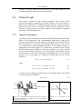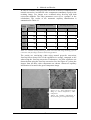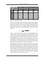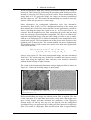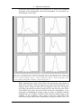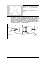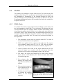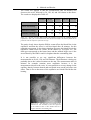
Download fulltext01 - DiVA Portal

Skin Capillary Ensemble Visualisation
and Computation
Ingemar Fredriksson
2004-03-10
LiTH-IMT/BIT20-EX--04/360--SE
Linköpings tekniska högskola
Institutionen för medicinsk teknik
ISRN: LiTH-IMT/BIT20-EX--04/360--SE
Datum: 2004-03-10
Svensk
titel
Visualisering och beräkning av hudkapillärer
Engelsk
titel
Skin Capillary Ensemble Visualisation and Computation
Författare
Ingemar Fredriksson
URL http://www.ep.liu.se/exjobb/imt/bit20/2004/360/
Uppdragsgivare:
Rapporttyp:
Rapportspråk:
Göran Salerud, IMT
Examensarbete
Engelska
Sammanfattning
Abstract
The aim of this thesis was to develop an objective and automatic method for identifying
capillaries in microscope images of the skin. Furthermore, statistical data about the
identified capillaries and the capillary distribution should be computed and stored in a
database. The method was implemented using the platform independent programming
language Java. An analysis of microscope improvement using various polarization filter
setups and wavelength filters has also been performed, as well as a pilot study of the effect
of applying a local anaesthetic cream on the skin.
The method is developed and aimed at research on various pathological skin conditions
affecting the capillary distribution. Hypertension, diabetes, inflammation, ischemia,
connective tissue disease, and erythromelalgia are all examples of diseases or pathological
conditions which are supposed to affect the distribution of the skin capillaries.
Nyckelord
Keywords
Microscopy, Capillary, Skin, Triangulation, Polarization, Image processing, Java
Bibliotekets anteckningar:
Abstract
Abstract
The aim of this thesis was to develop an objective and automatic method for
identifying capillaries in microscope images of the skin. Furthermore,
statistical data about the identified capillaries and the capillary distribution
should be computed and stored in a database. The method was implemented
using the platform independent programming language Java. An analysis of
microscope improvement using various polarization filter setups and
wavelength filters has also been performed, as well as a pilot study of the
effect of applying a local anaesthetic cream on the skin.
The method is developed and aimed at research on various pathological skin
conditions affecting the capillary distribution. Hypertension, diabetes,
inflammation, ischemia, connective tissue disease, and erythromelalgia are
all examples of diseases or pathological conditions which are supposed to
affect the distribution of the skin capillaries.
Acknowledgements
Acknowledgements
First of all I would like to thank my supervisor and examiner Göran Salerud
for his support and for showing a great interest and participation in my
work, and also for taking time for random chat. My vice supervisor Erik
Häggblad deserves a special thank for all practical tips and help with the
material, the study, and theoretical details. I would also like to thank Håkan
Rohman who gave me some practical tips with the microscope and the
polarizing filters. Other people who have eased my work are my
“roommate” Tobias Lindbergh, the factotum Michail Ilias, my master thesis
pals Mikael Svärd and Robert Holgersson, and all other nice men and
women who have made me feel welcome here at IMT.
Sv. Ps. 59
Linköping, February 2004
Ingemar Fredriksson
Table of Contents
Table of Contents
Glossary .........................................................................................................1
1
Introduction ............................................................................................3
2
Background ............................................................................................5
3
4
2.1
Skin Capillaries and Optical Properties of the Skin.......................5
2.2
Polarized Light...............................................................................7
2.2.1
Types of Polarization .................................................................7
2.2.2
Unpolarized Light ......................................................................9
2.2.3
Optical Components with Polarization Properties .....................9
Material ................................................................................................13
3.1
Microscope...................................................................................13
3.2
Computer......................................................................................14
Methods and Results ............................................................................15
4.1
Software .......................................................................................15
4.1.1
Microscope Images ..................................................................16
4.1.2
Pre-Processing..........................................................................16
4.1.3
Capillary Identification ............................................................22
4.1.4
Pattern Analysis........................................................................25
4.1.5
Database ...................................................................................30
4.1.6
JavaCap Features......................................................................30
4.2
4.2.1
Software Reliability .....................................................................34
Threshold Sensitivity................................................................34
Table of Contents
4.2.2
4.3
Hardware......................................................................................37
4.3.1
Microscope ...............................................................................37
4.3.2
Immersion Oil ..........................................................................38
4.3.3
Polarizing Filters ......................................................................39
4.3.4
Wavelength Filters ...................................................................41
4.4
4.4.1
5
Platform Independency ............................................................35
Studies..........................................................................................44
EMLA Study ............................................................................44
Discussion and Future Extensions........................................................47
5.1
Discussion ....................................................................................47
5.2
Future Extensions.........................................................................48
References....................................................................................................51
Appendices...................................................................................................53
A
Project Plan ..........................................................................................53
B
Requirement Specification ...................................................................71
C
User Manual .........................................................................................85
D
Test Images ........................................................................................111
E
Database Definitions ..........................................................................115
Glossary
Glossary
Artery, arteriole – Blood vessels which deliver blood from the heart to the
cells. The arterioles are the smallest arteries, and thus located closest to
the capillaries.
Base-64 encoding – Encoding technique which converts all characters of a
binary string to the secure 64 character subset of ‘A’ to ‘Z’, ‘a’ to ‘z’,
‘0’ to ‘9’, ‘+’, and ‘/’. That is done by concatenating three 8-bit groups
(three normal binary characters) to four 6-bit groups. These four 6-bit
groups are then translated to the characters above. The technique is
useful when no quote marks or other special characters are allowed,
e.g. in a database.
Capillary apex – The top loop of a skin capillary.
Circumcircle – The circle which totally circumfuses a given
triangle and touches all three corners of the triangle.
Dermis – The skin layer beneath the epidermis.
Circumcircle
Dorsal – The back or top of for example a foot or hand.
EMLA® – Local anaesthetic cream, sold at regular drugstores.
Epidermis – The thin superficial layer of the skin, normally about 70-180
µm thick and optically quite transparent in the visible spectra
[Anderson and Parrish 1982].
Erythromelalgia – Disease characterized by burning pain and high skin
temperature in distal parts of the body [Mørk, Kvernebo et al. 2002].
GUI – Graphical User Interface
ImCap – The analysing platform developed during PhD Claes Asker’s
work with his thesis “Computer Assisted Video Microscopy in
Characterisation of Capillary Ensembles” [Zhong, Asker et al. 2000].
IMT – Department of Biomedical Engineering, Linköpings universitet.
1
Glossary
In vivo – Measurement “in the living body”, the opposite of in vitro,
measurement “in an artificial environment” such as a test tube.
In vitro – See in vivo
Ischemia – Pathological state in which the blood cells are mechanically
obstructed, e.g. by narrowed arteries or inflammation [Spraycar 1990].
Java – Platform independent object oriented programming language
developed by Sun Microsystems.
Java VM – The Java Virtual Machine is the layer between a running java
application and the operating system which is needed in order to run
java applications.
JavaCap – The new platform independent analysing platform of ImCap
developed during this project.
JBuilder – Free development environment for Java used during the
software development of the project.
NIH Image – A public domain image processing and analysis program
originally developed for the Macintosh by the Research Services
Branch (RSB) of the National Institute of Mental Health (NIMH), part
of the National Institutes of Health (NIH). It was later on also
transferred to an open source Java project.
http://rsb.info.nih.gov/nih-image/index.html
NIR – Near Infra Red light, about 770-3000 nm.
ROI – Region Of Interest
Vein, venule – The blood vessels which return the blood from the cells to
the heart. The venules are the smallest veins, and thus located closest
to the capillaries.
Volar – The underside of for example an arm.
Wrist – sv. “handled”
2
1 – Introduction
1
Introduction
Capillary microscopy is a method to visualize the top loops, or actually the
red blood cells in the loops, of the capillaries located in the skin. The
technique is mostly used in order to measure parameters such as diameter
and blood flow in the individual capillaries in order to characterize and
diagnose various diseases. Hypertension, diabetes, inflammation, ischemia,
connective tissue disease, and erythromelalgia are diseases or pathological
conditions which all have some impact on those parameters [Asker 2000].
The technique has consequently been used to diagnose those conditions.
However, when diagnosing skin diseases not only the parameters of the
single capillaries are of interest, but also more global parameters like
capillary distribution could be of great importance. The analysis of the
global distribution in capillary ensembles was the focus of Claes Asker’s
PhD thesis [Asker 2000]. Part of his work was to develop an application
which made the analysis of the capillary ensembles automatic, and thus, in a
sense, objective. A major part of this master thesis was to improve that
method of identifying capillaries and computing the statistics wanted. That
was achieved by implementing a new application, with improved
functionality, using a platform independent programming language.
The capillaries were identified in microscope images from in vivo
measurements, and it was also investigated how polarization filters affect
those images, and how various light sources affect the images. Finally, the
application was used in one pilot study of how EMLA®, a local anaesthetic
cream, affects the capillaries.
In the beginning of the project, two documents were created. The first, the
Project Plan, describes how the project should be carried out, and the
project has then followed that plan. The other document, the Requirement
Specification, specifies the detailed requirements of both the application
built and the analyses made. The two documents can be found in
Appendix A and Appendix B, respectively.
The target group for this report is first of all persons who will use the
JavaCap application in research, but also students and others who have an
interest in the topics of the report. Fundamental knowledge in any or all of
the topics image processing, optics, and skin anatomy will be helpful when
reading the report.
Keywords: Microscopy, Capillary, Skin, Triangulation, Polarization,
Image processing, Java
3
2 – Background
2
Background
Some background theory needed for the understanding of the report is
located in this chapter.
2.1
Skin Capillaries and Optical Properties of the Skin
The smallest blood vessels in the body are called capillaries and they are
systematically located between the arterioles and the venules. Due to their
primary task, which is to exchange nutrients and waste between the blood
and the tissue, capillaries are found near almost every cell in the body and
the skin is no exception.
The skin capillaries are located in the papillary region in the dermis, see
Figure 2.1. The dermis is a 1000-4000 µm thick layer which mainly consists
of connective tissue, but also blood vessels, glands, and hair follicles. The
most superficial layer of the skin is called epidermis and is located above
the dermis (epi- = above). The epidermis is about 60-180 µm thick. The
wave-formed papillary region with the capillaries is the region closest to
epidermis and the capillary apexes are thus located at a depth of 60-200 µm.
[Tortora and Grabowski 2000]
Epidermis
~60-200 µm
Papillary
region
Capillary
Dermis
Figure 2.1 – Schematic view of the skin and its blood vessels.
5
2 – Background
The epidermis contains four different cell types. A majority of the cells are
keratinocytes which produces keratin, but from an optical point of view, the
melanocytes which produces melanin is the most interesting cells. Melanin
is a brown-black pigment which contributes to skin color and absorbs UV
light. An absorption spectra of melanin is shown in Figure 2.2a. Except
from the melanin, the main absorber of visible light in normal skin is blood,
or more precisely, the hemoglobin in the blood. The two types of
hemoglobin which are present in the blood are oxy-hemoglobin and deoxyhemoglobin. They have absorption spectra which differ slightly, but both
have absorption peaks at 410-440 nm and 520-580 nm [Tuchin 1997], see
Figure 2.2b. Mostly due to these two absorbers, the penetration depth of the
light in skin will be limited. In fair Caucasian skin, the penetration deep is
dependent of the wavelength according to Table 2.1.
a
b
Figure 2.2 a) – Absorption spectra of melanin. b) – Absorption spectra of oxy-hemoglobin
(solid line) and deoxy-hemoglobin (dashed line). The most interesting parts in these
spectra are the peaks in the green-yellow interval (520 – 580 nm). Values from [Prahl
1999]
Wavelength (nm)
250
280
300
350
400
450
500
600
700
800
Depth (µm)
2
1.5
6
60
90
150
230
550
750
1200
Table 2.1 – Approximate depth for
penetration of optical radiation in
fair Caucasian skin to a value of 1/e
(37%) of the incident energy density.
[Anderson and Parrish 1981]
In order to acquire capillary images with good visible capillaries, it is
convenient to use light with a wavelength which corresponds to any of the
absorption peaks of hemoglobin. The first interval to consider is thus 410440 nm, which contains the first high absorption peaks of hemoglobin.
According to Table 2.1, light at this wavelength has lost about 70% or more
of its intensity when reaching capillaries located at a depth of 150 µm.
Considering that the light has to return up through the skin again, almost all
intensity is then lost why the use of this wavelength interval is probably not
6
2 – Background
feasible. The other interval at 520-580 nm is more interesting since the
penetration depth for this interval is much greater.
2.2
Polarized Light
The nature of light has long confused mankind. The ancient Greeks
proposed that light is composed by particles, photons. The wave theory of
light was first proposed by Christian Huygens in the late 1600s. Nowadays,
both theories are used to explain the light, and the following sections
describe a special property of light using the electromagnetic approach,
polarization. [Freudenrich 2004]
2.2.1
Types of Polarization
According to the four equations of Maxwell [Nordling and Österman 1999],
which is the foundation of the electromagnetic light theory, light can be
described comprising an electric field and a magnetic field. Those fields are
best described as two vectors, E and B, which behave as waves. The vectors
are perpendicular to the propagation direction of the light, and they are
orthogonal to each other, Figure 2.3. Furthermore, given the electric field E,
B can be determined via Maxwell’s equations, and vice versa. Hence only E
is part of the discussion from now on. In the figures and formulas used in
this chapter, the z-axis is the direction of propagation, the x-axis is vertical
and the y-axis is horizontal, as in Figure 2.4. Using those axes, E can be
written as
E( x, y, z , t ) = E x xˆ + E y yˆ
(2.1)
E x ( x, y, z , t ) = Ax cos(ωt − kz + φ x )
(2.2)
E y ( x, y, z , t ) = Ay cos(ωt − kz + φ y )
(2.3)
where
Ax and Ay are the amplitudes and φx and φy are the phase angles from which
the relative phase is defined as
φ = φ y − φx
E
B
Propagation of light
(2.4)
x
y
z
Figure 2.3 – Illustration of the E and B vectors of light at
fixed time. E and B are perpendicular to the propagation of
light and to each other.
7
Figure 2.4 – Orientation of the
axes
2 – Background
The general case of polarization is described by equations (2.1)-(2.3). For a
fixed value of z the electric field vector describes an elliptic motion, as in
Figure 2.5a, and is therefore called elliptically polarized light.
For the special case of φ = 0 or φ = π, the light is linearly polarized, also
called plane polarized. In this case, Ey is proportional to Ex:
Ey =
Ay
Ax
Ex
(2.5)
for φ = 0, or
Ey = −
Ay
Ax
Ex
(2.6)
for φ = π. When z is fixed, E describes a harmonic motion along a line, as
shown in Figure 2.5b.
If φ = ± π / 2 and Ax = Ay, the light is said to be circularly polarized, see
Figure 2.5c. Ex and Ey can then be written as
E x = A cos(ωt − kz + φ x )
E y = A cos(ωt − kz + φ x ± π / 2)
(2.7)
= m A sin(ωt − kz + φ x )
which describes a circular movement of E. Circularly polarized light can be
either right circularly polarized (RCP) or left circularly polarized (LCP). It
is RCP when φ = +π / 2, since Ey then leads Ex by π / 2 rad, i.e. it reaches its
maximum a quarter of a cycle before Ex and thus describes a clockwise
motion in the x-y plane. The opposite is true for LCP. The same discussion
can be made for elliptically circular light, and is then called REP and LEP.
[Klein and Furtak 1986]
Ay
y
x
Ax
x
Ay
y
Ax
E
Ay
y
E
a
x
Ax
E
b
c
Figure 2.5 – The motion of the electric field E for three types of polarized light with fixed z. a) shows
the general case of equations (2.2) and (2.3) called elliptically polarized light. b) shows the special
case where φ = 0. E here oscillates along the line and the polarization type is thus called linear
polarization. c) shows the special case where Ax = Ay and φ = ± π / 2. The electric field varies along
the circle and the light is called circularly polarized.
8
2 – Background
2.2.2
Unpolarized Light
From a microscopic point of view, all light is polarized since a microscopic
light source such as an atom emits light with a well defined polarization
state. Unpolarized light is the result of many microscopic light sources with
various polarization states and thus exist in a macroscopic context only.
From a macroscopic point of view, the light is linearly polarized when all
microscopic parts of the light have the same polarization plane, it is
circularly polarized when all microscopic parts are circularly polarized in
the same direction and so on. Macroscopic light could also be partially
polarized, i.e. one dominating polarization plane. [Klein and Furtak 1986]
2.2.3
Optical Components with Polarization Properties
Polarized or partially polarized light is not very uncommon in daily life.
The light emitted from any LCD display is for example linearly polarized,
and light reflected from smooth interfaces is partially polarized in the plane
perpendicular to the reflection surface. Even the blue sky is partially
polarized, more polarized when the angle between the horizon and the sun
is small.
Special optical components exist which affect the polarization. The most
common is the linear polarizing filter. Such filters are oriented in one
direction and transmit the part of the light which is polarized in that
direction only. Therefore, an ideal linear polarizing filter transmits 50% of
the incoming light intensity if the light is totally unpolarized. In reality, the
filters however transmit only about 30-40% due to absorption and
reflections in the filter.
Circular polarizing filters are a bit more
complex. It would be natural to assume
that such filters transmit circular
polarized light only, but that is not the
case. They are composed by two steps;
the first step is an ordinary linear filter
and the second step converts the linear
polarized light to circular polarized. The
component
which
performs
this
“conversion” is called a quarter-wave
plate and a simple description of such a
component is that it consists of two axes;
one fast and one slow. Now consider the
illustration in Figure 2.6. The electric
field of the incident light, which is
linearly polarized, is at an angle of ψ =
45° with respect to the axes of the wave
plate and E can then be expressed as
Ay
LCP
Ax
y slow
ψ = 45°
E
Figure 2.6 – Illustration of the linear
to circular polarization conversion
using a quarter-wave plate. The
electric field of the incident linearly
polarized light is at an angle of 45°
with respect to the axes of the
quarter-wave plate.
E x = A cosψ cos ωt
E y = A sinψ cos ωt
9
x fast
(2.8)
2 – Background
After the transmission through the quarter-wave plate, there will be a
common phase shift φ´ and a relative phase shift of –π / 2 between the fast
and the slow axes. With A´ = Acos 45° = Asin 45°, E is expressed as
E x = A´cos(ωt − φ´)
E y = A´cos(ωt − φ´−π / 2)
(2.9)
= A´sin(ωt − φ´)
The transmitted light is in other words circularly polarized (compare with
eq. 2.7). The same discussion could be made for ψ ≠ 45°, and the result
would then be elliptically polarized light.
Circular polarization filters can be used to block reflected light when used
as in Figure 2.7. The changes of the electric field E during the passage
through the quarter-wave plate, before and after the reflection are shown in
Figure 2.8.
Linearly
polarized light
Circular
polarizing
filter
Unpolarized
light
Circularly
polarized light
Quarter-wave
plate
Linear
polarizing filter
Reflecting
surface
10
Figure 2.7 – Illustration of how a
circular polarizing filter can be used in
order to block reflected light. The
unpolarized light is filtered to linear
polarized, in the direction parallel with
the plane of the paper and perpendicular
to the direction of the light beam, in the
first passage through the linear filter.
The linearly polarized light is then
converted to RCP light by the quarterwave plate. When the light is reflected, it
is changed to LCP and in the second
passage through the wave plate it is
converted back to linearly polarized
light, but this time with the polarization
direction perpendicular to the paper
plane. The light is thus blocked when it
reaches the linear polarizing filter the
second time.
2 – Background
fast
slow
a
b
c
d
Figure 2.8 – The figures above illustrates why reflected light will be blocked using a
circular polarizing filter. A light wave with the E-vector projected on the slow and the fast
axes is shown, that is to say, the true E-vector is the resultant of the two components
shown in the images. The wave in a) is the linear polarized wave after the linear polarizing
filter. The wave in b) is the wave after the first pass through the quarter-wave plate. The
slow component is now λ/4 after the fast (compared to a), and the wave is left circular
polarized. The wave in c) is the reflected wave. The slow component is λ/4 ahead of the
fast, and the wave is right circular polarized. The wave in d) is the wave after the second
pass through the quarter-wave plate. The phase difference is λ/2 relative to a, and the
wave is again linear polarized, but the polarization angle is twisted 90°. That wave will be
blocked in the return through the linear polarizing filter.
11
3 – Material
3
Material
The material used in the project is described in this chapter.
3.1
Microscope
The microscope mostly used during the project, Scalar USB Microscope
M2 (Scalar Corporation), is a handheld microscope marketed for a wide
spectrum of costumers. The
microscope is connected to the
computer via the USB port and
the images are acquired via the
TWAIN interface like most
scanners and digital cameras.
The lens used gives a
magnification of about 200
(based on a 14 inch screen) so
that an image of size 640 × 480 Figure 3.1 – The USB microscope
pixels corresponds to about
1.6 × 1.2 mm.
Another microscope, Microvision MV 2100 (Finlay Microvision Co. Ltd.),
was tested for comparison. The images from this microscope have a
resolution of 760 × 564 pixels and about the same order of magnification as
the USB microscope.
When acquiring images of the skin, reflections in the skin are very
dominant and complicate the detection of the capillaries. In order to get rid
of these reflections, two methods were tested. The first method was to use
immersion oil (immersion oil for microscopy, Nikon, MXA20235,
refraction index = 1.515 (23°C)).
The second method was to use polarizing filters. Tech spec™ linear
polarizing laminated film was used, a filter with an even and rather high
(38% average) transmission in the visible spectra. Circular polarizing filters,
which are a combination of a linear filter combined with a ¼λ retarder, was
also used (3M, 37% transmission, neutral color).
Three green band-pass wavelength filters (Rosco Laboratories Ltd.) were
tested with the microscope. The filters were named: #86 – pea green, #89 –
moss green, and #388 – gaslight green. When measuring the wavelength
13
3 – Material
spectra from the original light source and from the light source together
with the various filters, a spectroscope was used (AvaSpec 2048-5-RM,
serial number 0309006SF). An integrating sphere (Oriel, model number
70461) was also used and the integrating sphere and the spectroscope was
connected via a 200/230 µm glass fibre.
3.2
Computer
The computer used for development of the JavaCap application, testing of
JavaCap, and finally computation of the results using JavaCap was a Dell
Optiplex GX270 computer with an Intel® Pentium 4 2.4 GHz processor and
512 MB of RAM. The operating system was Microsoft Windows XP home
edition. JavaCap is however platform independent and was also tested on a
Macintosh G3 with a 350 MHz PowerPC processor with Mac OS X, and on
a Sun Solaris 9 machine.
The programming environment used during the software development was
Borland JBuilder (personal edition). It is a free Java development
environment available at the Borland web page (www.borland.com).
As coding references, the Java™ 2 Platform, Standard Edition, v 1.4.2 API
Specification was used as well as the book Core JAVA 2, Volume 1 –
Fundamentals [Horstmann and Cornell 2003]. Various internet resources
were also consulted.
14
4 – Methods and Results
4
Methods and Results
The methods used and the results obtained in the project are described in
this chapter. The chapter is divided into four sections, were the first section
describes the software development and the resulting JavaCap application
and the second chapter contains some tests of the application. The third
section describes the methods used during the hardware analysis, and the
fourth section describes the methods used during the EMLA® study and the
results of that study.
4.1
Software
The previous ImCap application contained five image processing steps and
those were: greyscale converting, alpha trimmed mean filtering, band-pass
filtering, thresholding, and median filtering. They are implemented in
JavaCap, with some modifications, and a description of each step as well as
motivations of their presence in the application and possible improvements
and/or alternatives, are presented in section 4.1.2 – Pre-Processing. The
capillary identification process is described in section 4.1.3, and then
section 4.1.4 – Pattern Analysis follows, motivating and describing the
capillary ensemble analysis. Section 4.1.5 describes the database
functionality of the application and the chapter ends with a description of
other features in JavaCap, such as options and histograms (section 4.1.6).
Section 4.1.1 discusses the contents of the microscope images, in order to
motivate the image processing steps.
Almost all code of the JavaCap application was written from scratch. Before
the coding started, it was assumed that a lot of code could be more or less
copied from the old ImCap application and from the Java version of NIH
Image (ImageJ). The reasons not reusing code from ImCap are the lack of
code documentation, and since the old code was written in C++ it contains a
lot of pointers making the code difficult to comprehend. The reason not
using code from ImageJ is the use of a very powerful but complex image
handling system, which would be unnecessary to implement in JavaCap.
The application is only supposed to be used in a scientific environment,
why functionality is prioritized before automatic processes. See also the
User Manual in Appendix C for a description how to use the application.
15
4 – Methods and Results
4.1.1
Microscope Images
The images from the microscope are
captured as 24-bit color images. In
most parts of the human skin, the
capillaries are perpendicular to the
skin surface, and the part of the
single capillaries shown in the
images are just the apex of the
capillary loop, appearing as a dark
red spot in the image. A typical
capillary image is shown in Figure
4.1.
4.1.2
Figure 4.1 – Capillary image. The dark
spots are the capillary apexes.
Pre-Processing
The first image processing step converts the color image into an 8-bit grey
scale image. The color image will after that only be used as a reference. The
greyscale conversion will lead to loss of data, but the following image
processing will be much simpler if performed on greyscale images. In order
to reduce the drawbacks of this data reduction, and even turn it into an
advantage, it can manually be adjusted how much each color band (red,
green, blue) will affect the resulting grey scale image. If these factors are
chosen in a favourable way, the contrast between the capillaries and the
background can be enhanced. Best results are obtained if the green
component of the image is allowed to dominate the greyscale conversion.
The greyscale conversion is in detail performed according to the following
steps:
1. The conversion factors of the three color bands are chosen as values
between 0 and 1, with the sum of the factors automatically set to 1.
2. For each pixel in the color image, the values of the three color
components are retrieved.
3. The resulting grey value of the pixel is set to the sum of the pixel
values multiplied with the conversion factors:
GrayValue = redComponent × redFactor +
greenComponent × greenFactor +
blueComponent × blueFactor
(4.1)
The ability to change the color factors is a new feature in JavaCap. It
reduces the drawbacks of the data reduction since it keeps the information
about the capillaries and removes redundant information. If a proper green
wavelength filters are used, most information about the capillaries is in the
green color band and little or no capillary information is lost in this step.
16
4 – Methods and Results
In order to evaluate if this greyscale conversion is better in comparision to a
normal conversion, in which all color components contributes equaly to the
resulting image, five images were evaluated using JavaCap with both
conversion methods. The other parameters were set to “optimal” in the
calculations. The results of the automatic capillary identification is
summarized in Table 4.1.
Total
number of
capillaries
Missed caps.
1
63
16
1
0
1
2
126
27
1
1
1
3
117
7
1
3
1
4
54
8
6
1
1
5
64
26
8
12
6
Image
no.
Normal conversion
JavaCap conversion
False caps.
Missed caps.
False caps.
Table 4.1 – Results of using normal greyscale conversion and using JavaCap greyscale
conversion. The five images used are shown in Appendix D.
The results are convincing; when using normal greyscale conversion,
JavaCap fails to detect 20% of the capillaries in average, compared to 4%
when using the JavaCap conversion. Furthermore, less false capillaries are
detected when using the JavaCap conversion. See also Figure 4.2, where the
images from all three color components are shown. Almost all capillary
information is located in the green component image.
a
b
Figure 4.2 a) – Red component of the
image. b) – Green component c) – Blue
component.
Almost all capillary information is
located in the green component image.
c
17
4 – Methods and Results
The aim of the next image processing step is to reduce the noise in the
image without removing the capillary edges. A simple running average
filter removing Gaussian noise could be considered. Another approach is to
use a median filter which is optimal for removing long-tail distributed noise.
An α-trimmed mean filter is a compromise between the two, and a
mathematical definition of the filter is found in equation 4.2. Suppose the
grey value pixels in a convolution window Wij around the pixel xij are sorted
in an ascending order into: x1 ≤ x2 ≤ … ≤xN, where N is the size of the
window. The α-trimmed mean filter is then defined as,
xˆ ij =
N −αN
1
∑ x k , 0 ≤ α < 0 .5
N (1 − 2α ) k =αN +1
(4.2)
where α = 0 results in a normal moving average filter and lim α → 0.5
results in a median filter. A simple modification of the filter can also
produce an additional edge enhancing effect. It is done by using two
different α-values,
xˆij =
N −α 2 N
1
∑ x k , 0 ≤ α 1 , α 2 < 0 .5
N (1 − α1 − α 2 ) k =α1N +1
(4.3)
When α1 = 0.5 and α2 = 0, the resulting filter has an effect as a maximal
filter, and when α1 = 0 and α2 = 0.5 the effect is a minimal filter. The filter
used in JavaCap is closer to a minimal filter than to a maximal and does
enhance the dark capillaries a bit, which must be considered in later
processing steps.
The actual filter used in JavaCap is defined as
xˆij =
N − 2 / 9 N 
1
∑ xk
N − 1 / 9 N  − 2 / 9 N  k = 1 / 9 N +1
(4.4)
The size of the convolution window can be changed in JavaCap. A window
of size 3 × 3 (N = 9) seems to work fine and is thus used as default. It
results in a quite strong smoothing effect reducing the Gaussian noise
effectively. [Zhong, Asker et al. 2000]
The result of an α-trimmed filter on five images is showed in Table 4.2. The
result is compared to the result obtained when not using the filter. The effect
is small, but less false capillaries are identified when using the filter.
18
4 – Methods and Results
Total
number of
capillaries
Missed caps.
1
63
0
1
0
1
2
126
0
4
1
1
3
117
1
2
3
1
4
54
3
2
1
1
5
64
9
12
12
6
Image
no.
No filter
α-trimmed filter
False caps.
Missed caps.
False caps.
Table 4.2 – Results of using α-trimmed mean filter compared to not using it. The five
images used are shown in Appendix D.
The next step is to achieve a uniform background and enhance the capillary
edges. Since the background is of low spatial frequency, and the capillary
edges are of high spatial frequency, low frequencies should be filtered.
Thus, a high-pass filter is used. A high-pass filter can be implemented by
subtracting an image with its own low-pass filtered image. The low-pass
filter process is performed by convolving the image with a Gaussian kernel
defined by
f ( x, y ) =
1
2πσ
2
e
−
( x − x0 ) 2 + ( y − y 0 ) 2
2σ 2
(4.5)
where x0, y0 is the center of the kernel and σ is the spatial standard deviation
[Weisstein 1999a]. The low-pass cut-off frequency is controlled by σ where
a smaller σ implies a larger cut-off frequency. An ideal Gaussian kernel has
infinite size, but since that is impossible to implement, the kernel size can
be adjusted between 3 × 3 and 35 × 35 pixels in JavaCap. The σ-value is
then calculated to get the sum of the kernel to about 0.99. If the sum is
smaller than 0.99, it implies too big σ and is then decreased until the sum is
greater than 0.99. Decreasing σ when the sum is too large makes σ smaller
for smaller kernels, and the kernel size thus controls the cut-off frequency
indirectly – the cut-off frequency is larger for smaller kernels.
Transforming the low-pass filter to a high-pass filter is done by subtracting
the original image with the low-pass filtered image. The kernel size controls
the high-pass cut-off frequency; a larger kernel implies a higher cut-off
frequency for the high-pass filter. A high cut-off frequency is necessary in
order to remove illumination differences in the background, but a too high
cut-off frequency can remove some blurred capillaries. The process also
creates a white border surrounding the image, with a width of half the
kernel size, and is therefore a reason of using a small kernel size and a low
cut-off frequency. A kernel size of 13 × 13 pixels is used as default in
JavaCap, and that size is based on empirical tests.
19
4 – Methods and Results
When performing the high-pass filtering, maximum contrast in the image is
preserved. This is done by performing all operations with double precision,
instead of using the 255 discrete greyscale values. When transforming the
image back to a 255 greyscale image, the values are linearly transformed
into the range 0 to 255. This makes the thresholding less sensitive since the
discrete values are spread over a wider range.
Other alternatives for background subtraction exist. One alternative
described by Russ [1995] is to fit a background function to the image and
then subtract the result of the same function. In this application it could be
done by dividing the image into a grid of size n × m. For each of the n × m
sections, find the brightest pixel, then interpolate the pixels and put them
back into an image representing the background. The idea is to subtract the
acquired background image from the other image in order to get an image
with an even background. Two different methods for the interpolation were
tested in the project. The first method sets all the pixels in the sections to the
brightest pixel in that section. The second method was more sophisticated.
The brightest values of all sections was used to fit a third order polynomial
with ten coefficients
P( x, y ) = a0 + a1 ⋅ x + a 2 ⋅ x 2 + a3 ⋅ x 3 + a 4 ⋅ xy +
a5 x 2 y + a6 ⋅ xy 2 + a7 ⋅ y + a8 ⋅ y 2 + a9 ⋅ y 3
(4.6)
using a least square fit. The entire background image was then calculated
from (4.6). The result using any of these two methods was however much
worse than using the high-pass filter and they were therefore discarded
without further testing or improvements.
The result of the background elimination using a high-pass filter is shown in
Figure 4.3. Notice the resulting image is quite grainy.
a
b
Figure 4.3 a) – α-trimmed image, window size 3 × 3. b) – High-pass filtered image with
a kernel size of 13 × 13.
Before thresholding the image, an ordinary mean filter is applied. The aim
of this operation is to make dark areas more evenly dark, and bright areas
more evenly bright, and thus eliminate the graininess of the high-pass
filtered image. In ImCap, this step was not present, but the background
equalization step was performed by a band-pass filter instead of a high-pass
filter. The result of a high-pass filter and this mean filter is approximately
20
4 – Methods and Results
the same as a band-pass filter, and this approach is chosen since the
parameters of the two filters are easier to control when adjusted separately.
The window size of the mean kernel can be adjusted, and the default value
is set to 5 × 5 pixels, based on empirical tests.
Table 4.3 shows the results of applying the filter to five images. Without the
filter, 16% of the capillaries are missed by JavaCap, and this should be
compared with 4% if it is used.
Total
number of
capillaries
Missed caps.
1
63
17
1
0
1
2
126
10
0
1
1
3
117
11
1
3
1
4
54
7
3
1
1
5
64
21
9
12
6
Image
no.
No filter
Mean filter
False caps.
Missed caps.
False caps.
Table 4.3 – Results with and without mean filtering. The five images used are shown in
Appendix D.
Thresholding the image is performed in order to make a binary image for
further analysis. Thresholding means that all greyscale values greater than
or equal to the threshold value become white, and all lower values become
black. The threshold value can be adjusted manually (between 0 and 255).
Although this threshold value could be computed automatically, it should be
adjusted manually for optimal results. A mean filtered image and its
processed image is shown in Figure 4.4.
a
b
Figure 4.4 a) – Mean filtered image b) Thresholded image
Before the capillary identification process start, one more pre-processing
step remains. A simple median filter is run twice in order to reduce spike
noise. The size of the median window is 3 × 3 by default, but can be
changed if the image still contains much noise. The result of the median
21
4 – Methods and Results
filter is elimination of small isolated objects and smoothing of larger
objects. This also shrinks the objects in order to compensate for the
enlargement done by the α-trimmed mean filter.
Table 4.4 shows the results of using the median filter compared to not using
it. When not using the median filter, about twice as many capillaries are
missed, and the number of false capillaries is eight times higher.
Total
number of
capillaries
Missed caps.
1
63
5
2
0
1
2
126
3
18
1
1
3
117
14
15
3
1
4
54
5
16
1
1
5
64
9
29
12
6
Image
no.
No filter
Median filter
False caps.
Missed caps.
False caps.
Table 4.4 – Results of using the median filter step and not using it. The five images used
are shown in Appendix D.
4.1.3
Capillary Identification
To localize the black regions of the thresholded and median filtered image,
line scanning is used. Whenever a black pixel is found, the algorithm enters
a recursive state, looking in the neighbourhood for other black pixels. When
performing the line scan, only every second line and column is scanned.
This makes the scan almost four times faster than if every pixel would have
been scanned, and the objects missed are so small that they can not be
considered as capillaries. When entering the recursive state, all pixels in the
neighbourhood are scanned though.
The objects found must pass a number of criteria before they can be treated
as capillaries, and those steps are described below.
The first processing step is the use of a calibration measurement. The aim is
to remove objects which origins from dust particles on the microscope and
thus are present at the same location in all images. A calibration
measurement is a normal measurement preferably calculated from an image
of a white paper where the dust particles are stored as capillaries. All
objects in the image which corresponds to the “capillaries” of the
calibration measurement are then simply removed.
The second step removes very large objects, since they are certainly not
capillaries and the computation of the following steps will decrease if
removed. The upper limit of the size of the objects is 100 times the lower
limit which can be set in the application.
22
4 – Methods and Results
An optional third step deletes objects which are not filled and this is useful
if many small bubbles exist in the image.
Deleting objects which are artefacts arising from bubbles in the immersion
oil are performed in the fourth step. They are objects localized at the border
of larger bubbles. Due to these objects’ locations at the border of bubbles,
the greyscale value of each side of the object will differ markedly and the
aim is to remove objects which have large differences in greyscale values.
The algorithm is as follows: from every edge-point of the object, search is
performed in the four directions left, right, up, and down. When outside the
object in each direction, the greyscale value of the brightest out of the five
closest pixels in the current direction is stored. Then the difference is
calculated between left and right, and up and down, respectively. If the
difference in either of these two directions is greater than a threshold value,
increase a test counter. When this test is performed for all edge points, the
test counter is controlled. If the test counter is greater than one third of the
size of the object, the object is considered as a false capillary, and thus
rejected. Since it is only the edge points which are tested, objects which are
not very circular or quadratic have a harder time to pass the test, (they have
a higher concentration of edge points) which is good since this kind of
artefact objects often are more stretched than true capillaries. See also
Figure 4.5.
a
b
Figure 4.5 – The white object marked in a) is an artefact due to air in the immersion oil.
The edge of this object is enhanced by the high-pass filter and the result is two black
objects after thresholding and median filter as shown in the magnified image b). b) also
describes the algorithm; for the pixel P, which is an edge pixel, locate one pixel in each of
the four directions. The properties of these detected pixels are: they are outside the black
object and it is the brightest pixel of the five pixels closest to P outside the object and in the
current direction. The pixels in the directions left, right, up and down are marked as L, R,
U, and D respectively. The difference of the greyscale value is then calculated between L
and R , and U and D and the difference is compared to a threshold value.
The fifth step is to remove artefacts originating from undesired particles.
The idea is that the color of such objects differs from true capillaries. The
algorithm calculates the mean color of each object, or actually the mean
value of each color component (red, green, blue) of each object. In the
23
4 – Methods and Results
formula below, redi, greeni, and bluei is the red, green, and blue mean value
for each object, respectively. Ni is the number of pixels of object i and
redPixelValueij, greenPixelValueij, and bluePixelValueij are the red, green,
and blue pixel values for pixel j of object i.

1 Ni
=
red
redPixelValueij
 i
∑
N
j
=
1
i


1 Ni
 greeni =
∑ greenPixelValueij
N i j =1


1 Ni
bluei =
∑ bluePixelValueij
N i j =1

(4.7)
The mean values are sorted according to
red1 ≤ red 2 ≤ ... ≤ red M

 green1 ≤ green2 ≤ ... ≤ greenM
blue ≤ blue ≤ ... ≤ blue
1
2
M

(4.8)
where M = the number of objects. When this is done, the median color of all
objects is calculated, again for all three color bands.
redMedian = red M / 2 

 greenMedian = greenM / 2 

blueMedian = blueM / 2 
(4.9)
The sum of the quadratic distance for the three color bands to the median
color is then calculated for each object.
 (redMedian − red i )2 +
M 
2
sqDist = ∑  (redMedian − greeni )
i =1 
 (redMedian − bluei )2



+  ≤ threshold



(4.10)
If sqDist exceeds threshold, the object is rejected. This step could probably
be improved if the background was subtracted in the original color image,
since the color of the capillaries then would be more similar and the
threshold could thus be more accurate.
The sixth step is to merge objects which are very close to each other. There
is a high probability that those objects belong to the same capillary, and
therefore should be merged. This algorithm is very time consuming since
the distances between many points are calculated. Not only the center points
of the objects are considered, but all the points of the object. Objects with a
space between them which is less than three times the radius of the smallest
capillary allowed are merged together. This limit is chosen since it is not
likely that capillaries are tighter together than that. The size of the smallest
capillaries allowed can be adjusted in the application.
24
4 – Methods and Results
The seventh step is quite simple, it just removes all objects which are
smaller than the minimum size allowed for capillaries. This size can be
changed in the options dialog, and the default value is set to 100 µm which
is a value based on empirical tests.
The eighth and final step removes objects which are not at all circular in
shape. In JavaCap, a test is performed in order to evaluate if all points of the
object are close enough to the center of the object. The radius of the object,
supposing the object was a perfect circle, is calculated. The center of the
object is also calculated, by identifying the minimum and maximum x and y
coordinates of the objects and dividing by two. The actual test is then to
check that the distance from each pixel of the object to the center is less
than or equal to the calculated radius times a tolerance factor of 2.0. The use
of that value only removes the worst objects, but it could not be smaller
since some capillaries are quite stretched. If the test is fulfilled, the object is
considered to be a capillary.
After these eight steps, the automatic
capillary identification process is
done, and all remaining objects are
stored with their position and size.
An image with the identified
capillaries is shown in Figure 4.6. In
order to correct any mistakes
performed by the process, it is now
possible to manually add and remove
capillaries.
Figure 4.6 – The identified capillaries are
marked in the image.
4.1.4
Pattern Analysis
In order to obtain information of clinical use, statistics such as capillary size
and the capillary distribution in the image will be analyzed.
First capillary density (capillaries/mm²), capillary size, and the capillary
size uniformity are calculated. The capillary size stored is the mean size,
equation 4.11, and the standard deviation, calculated by equation 4.12.
meanSize =
standardDeviation =
1
N
N
∑ size
i =1
i
1 N
(meanSize − sizei ) 2
∑
N i =1
(4.11)
(4.12)
In all equations, N is the number of capillaries and sizei is the size of
capillary i.
25
4 – Methods and Results
The capillary size uniformity is calculated by
uniformity = 1 −
standardDe viation
meanSize
(4.13)
where uniformity = 1 means that all capillaries are equal in size, and a value
closer to 0 or even negative means a huge difference in size.
The shape of the capillaries is of minor importance when analyzing the
distribution, and therefore only size and position are stored for each
capillary. Actually, in the analyse made in this project, the size of the
capillaries is not considered either, even though that parameter could be of
great importance for the oxygen diffusion in the skin, since larger capillaries
are able to transport more blood and could thus support more tissue than
smaller capillaries.
The Krogh model is a simplified oxygen diffusion model described by
[Friedman 1986]. It describes the condition for an effective interaction in a
tissue metabolic process due to geometric proximity. Using this model the
basis for the analysis of the capillary ensemble will therefore be to
investigate the 2-dimensional capillary distribution. This is performed in
two ways. The first is the neighbour identification, and the second is the
triangulation and is described later in this section.
All capillaries registered in the image have a nearest neighbour capillary,
and those capillaries can be connected via an edge ei from the first capillary
to the second with a length li. All the edges in an image comprise a minimal
distance map, similar to that shown in Figure 4.7a. The average length of
the edges in the minimal distance map is calculated by
meanLength =
1 N
∑ li
N i =1
(4.14)
where N is the number of edges. The standard deviation and the uniformity
are given by
standardDeviation =
uniformity = 1 −
1
N
N
∑ (meanLength − l )
i =1
standardDeviation
meanLength
i
2
(4.15)
(4.16)
As seen in Figure 4.7a, the resulting map, or graph, is divided into many sub
graphs, and the minimal distance map is a local descriptor of the geometric
pattern, maybe a too local descriptor. In JavaCap, this is solved by
generating a minimal distance map in which also the second and the third
neighbours of each capillary are included, a third order minimal distance
map. Such a map is shown in Figure 4.7b, and that map clearly
demonstrates clusters of capillaries. The mean length, the standard
deviation, and the uniformity are also calculated by equations 4.14, 4.15,
and 4.16 (li is now the length of the second and third neighbour edge).
26
4 – Methods and Results
a
b
Figure 4.7 a) – Minimal distance map. The edge to the closest neighbour of each
capillary is shown. b) Minimal distance map with the edges to the three closest
neighbours.
The third order minimal distance map reveals a lot of information about the
capillary distribution, but it could still be a too local description. The natural
solution would be too calculate the (N – 1):th order minimal distance map.
Unfortunately, such a map violates Krogh’s diffusion model since the map
would contain edges connecting capillaries far from each other. The optimal
solution is to have a fully connected graph with as many, and as short edges
as possible, and no edges intersecting each other. The technique for solving
such problem is called triangulation and the result is a mutual distance map.
Triangulation methods are usually used for reconstructing surface meshes
based on a random or irregular set of sampling points. The aim is then to
establish the local adjacent relationship among the sampling points and then
use the relationship in order to derive an interpolation formula for the
surface reconstruction [Zhong, Asker et al. 2000].
The statistics derived from the triangulation is a measure of the global
distribution. The mutual distance is calculated by 4.14 and 4.15 (mean
length of the edges ± the standard deviation), and the distribution uniformity
is calculated by 4.16.
The triangulation method first implemented in JavaCap was the greedy
algorithm, which is built up of the following steps:
1. Create an array of all edges between all capillaries (one edge per
capillary pair).
2. Sort that array in ascending order, the shortest edge is first, and the
longest last.
3. Step through the array, starting with the shortest edge. Remove all
longer edges which properly intersect that edge. Edges properly
intersect each other if they have any common point except the start
and end points.
The algorithm is of complexity O(N2logN2) [Asker 2000] and tends to
contain as short edges as possible. At the border of the convex hull of the
27
4 – Methods and Results
triangulation a lot of long edges exist, see Figure 4.8a. Many of those long
edges would not exist if the image was larger, since capillaries on the other
side of the image border then would generate another triangulation without
these long edges. Therefore we have a delicate problem at the border of the
ROI, hard to solve accurately. The solution should contain statistical data,
derived both globally and locally, in order to calculate the probability of a
capillary which should change the triangulation edges. A proper solution of
the problem is left out in this project, but a simpler approach is presented
and implemented, and it seems to work acceptably. The algorithm simply
steps through the edges, starting with the longest edge, and removes the
edge as long as it is a border edge. The result of the triangulation after the
removal of the elongated border edges can be seen in Figure 4.8b.
a
b
Figure 4.8 a) – Greedy triangulation. b) – Greedy triangulation with elongated border
edges removed.
Other triangulation methods also exist. One is the optimal triangulation
method. It is defined to have the minimal sum of edge lengths. However,
since no general algorithms exist for optimal triangulation it is not
implemented in JavaCap. Besides, the result of the greedy method is often
very close to the optimal. [Asker 2000; Zhong, Asker et al. 2000]
Another common triangulation method is the Delaunay triangulation [Asker
2000]. The criterion for this triangulation is that no point of the point set
should be positioned inside the circumcircle of any other triangle of points.
This makes the angles of the triangles as large as possible and the edges will
be the edges between the natural neighbours (Voronoi neighbours) [Zhong,
Asker et al. 2000]. The triangulation could be computed in O(NlogN) time
[Leach 1992], but the algorithm used in JavaCap is of O(N4) complexity. It
is a straightforward algorithm and consists of the following steps:
1. Find all possible triangles in the capillary set, i.e. all triangles with
corners in three of the capillaries. This is done in O(N3) time.
2. For all triangles, calculate the circumcircle. The calculations are
based on equations (4.17-4.21) [Weisstein 1999a]:
x1
a = x2
x3
28
y1 1
y2 1
y3 1
(4.17)
4 – Methods and Results
2
2
x1 + y1
2
2
bx = x 2 + y 2
2
2
x3 + y 3
2
2
x1 + y1
2
2
b y = − x2 + y 2
2
2
x3 + y 3
cx =
cy =
bx
2a
by
2a
y1 1
y2 1
y3 1
x1 1
x2 1
x3 1
(4.18)
(4.19)
(4.20)
(4.21)
where xn, yn is the coordinate of the corner n (1 to 3) and cx, cy is the
center of the circumcircle. The radius is then calculated with
Pythagora’s theorem (a2 + b2 = c2).
3. For each such circumcircle, check if it contains any other capillary,
which is done in O(N) time. If this is true, remove the edges of that
triangle.
4. The remaining edges (no duplicates) results in the triangulation.
5. As in the greedy algorithm, elongated edges at the border are
removed.
An algorithm of less complexity is a future extension to the project if the
Delaunay method proves to be superior to the greedy algorithm.
a
b
Figure 4.9 Comparision of the triangulation methods. a) – Greedy triangulation.
b) – Delaunay triangulation
The edges marked in b) are examples of edges which differs from a), but as could be
seen, the differences are minimal, and the effect of the differences is even smaller. This is
however a healthy subject and the differences might be greater in pathological tissue.
It is possible to choose triangulation method in JavaCap and the results
normally do not differ significantly (see Figure 4.9). The Delaunay
triangulation could be considered as a better representation of the real world
29
4 – Methods and Results
since it chooses the natural neighbours and thus satisfies the Krogh model
better. For more information about natural neighbours, read about Delaunay
triangulation and Voronoi diagrams in [Asker 2000]. Something that would
motivate the use of the greedy algorithm is error sensitivity. The sum of the
lengths of the edges is a function of the vertex (capillary) positions – if a
vertex is moved, the sum will change. The important parameters calculated,
such as the distribution uniformity, are dependent of that sum. In order to
eliminate an error source, the error dependent of the vertex positions should
go towards zero when the error of the positions goes towards zero, which is
not always the case in the Delaunay algorithm [Zhong, Asker et al. 2000].
Which of the triangulation methods to use is still to be investigated, and the
greedy algorithm is used as default till then since it is faster.
4.1.5
Database
The information about the patients and the measurements is stored in a
MySQL database. The database consists of three tables, which can be found
in Appendix E.
The information stored in the patient table is the civic registration number
of the patient, the name, and the gender. The measurement table contains
both data such as date, part, and comments about the measurement, but it
also contains the parameters used in the computation of the measurement
and the capillaries. All the statistics about the measurements are stored in
the statistics table. JavaCap never reads from this table, it is only used in the
comparison of measurements in a database environment.
The relation between the patient and the measurement table is an 1-n
relation, meaning that a patient can have many measurements, but a
measurement can only belong to one patient. The relation between the
measurement table and the statistics table is a 1-1 relation, meaning that an
entry in the statistics table belongs to one specific measurement and vice
versa.
4.1.6
JavaCap Features
This section describes some of the many features of JavaCap. A user
manual, which in detail describes how to use the application, is presented in
Appendix C.
Figure 4.10 shows the main window of the JavaCap application. It consists
of four parts. At the bottom, a status bar is shown. At the top a menu is
shown from which all the commands can be executed and at the right, the
results and statistics are showed. The statistics are updated as soon as new
computations affecting the statistics are performed.
30
4 – Methods and Results
Figure 4.10 – The JavaCap main window.
To the top, there is a tab area, which is the most important part of the
application. Each tab contains an image of the process. The ‘original’ tab
contains the original colored image, the ‘greyscale’ tab contains the
greyscale image and so on. When clicking on a tab, the contents of the tab is
calculated and the tab is shown. Certain controls also appear in a toolbox
depending on the tabbed clicked. The controls shown are listed below:
•
No tab – Four buttons are shown, and they are: open a new image,
acquire an image from the TWAIN interface, open an old
measurement, and store measurement (not enabled). These four
buttons are always shown.
•
Original tab – A magnifying glass is added and shown for all tabs.
When the magnify button is selected, by clicking on the image, that
part of the image will be magnified. A button for calculating the
next step is also added.
•
Greyscale tab – Except the magnifiyng glass three slider controls are
also shown, one for each color band (red, green, blue). When
altering these sliders, the greyscale conversion factors are changed
and the image is updated (see section 2.1 and 4.3.4).
•
Alpha trimmed tab – A spinner control is shown. The value of the
spinner control controls the size of the window of the alpha trimmed
mean filter.
31
4 – Methods and Results
•
Background subtracted tab – Like the alpha trimmed tab, except that
the size of the band-pass kernel is altered with the spinner control.
See Figure 4.11a.
•
Mean filtered tab – Like the alpha trimmed tab.
•
Thresholded tab – A slider object controlling the threshold value is
shown.
•
Median filtered tab – Like the alpha trimmed tab.
•
Capillaries tab – Four checkboxes are shown controlling whether or
not to show the capillaries and/or any of the three closest
neighbours. The shown buttons are: ‘Delete capillaries’ which
deletes the selected capillary/capillaries, ‘Select capillaries’ which
enables selection of one or more capillaries by clicking in the
capillary image, ‘Draw capillary’ which enables the user to draw
new capillaries missed by the capillary identification process, and
two histogram buttons. The histogram buttons draws the histograms
of the capillary sizes and the neighbour distances, respectively. A
button from which it is possible to change the capillary identification
steps to use is also shown. The dialog for the capillary controls is
shown in Figure 4.11b.
•
Triangulation tab – A button which shows the histogram of the edge
lengths of the mutual distance map is shown, as well as two radio
buttons which select which triangulation method to be used, i.e.
greedy or Delaunay.
a
b
Figure 4.11 – Examples of the contents of the controls dialog.
a) – Background subtraction controls. b) – Capillaries controls.
As mentioned above, histograms can be shown for capillary size, neighbour
distances and mutual distance edge length. The histograms first divide the
value range into a number of intervals (between 10 and 50 intervals
depending on the number of values). Then, it counts the number of values in
each interval and, finally, bars representing the number of values in each
interval are drawn. The minimum, middle, and maximum values are shown
on the x-axis. A typical histogram is shown in Figure 4.12.
32
4 – Methods and Results
Figure 4.12 – Triangulation edge length histogram.
A number of options can be controlled in the options dialog (shown in
Figure 4.13). The Restore values button restores the options to the values
from the point when the options dialog was opened. The Default values
button sets the options to the pre-defined values.
Figure 4.13 – Options dialog
33
4 – Methods and Results
4.2
Software Reliability
Two formal tests have been performed in order to evaluate the reliability of
the JavaCap software. The first test was performed in order to evaluate the
sensitivity of the threshold value, which is to be manually adjusted for each
measurement. The second was to evaluate the platform independency.
In addition to the two formal tests, all functionality has been tested during
the development. The application has also been tested by the supervisor of
the project, and an early version was used in a laboratory moment in a
graduate course during the fall of 2003, where the functionality was tested
indirectly. Comparisons to the old ImCap application have also been done,
with satisfying results. The reason of not making that comparison more
formal and detailed is that ImCap requires images of a very special format,
which has not been possible to generate. The comparison was thus
performed with just two, very “nice”, images which are not representative.
A solid software test is only meaningful if it is performed by a person which
is not involved in the details of the development. Thus, such a test could not
be performed by the master thesis student, and since no one else has been
engaged, a thorough software test has not been performed.
4.2.1
Threshold Sensitivity
To evaluate the sensitivity of the threshold value, it was tested how many
capillaries were missed and how many false capillaries were present for
various threshold values in five different images. The results are shown in
Figure 4.14. The conclusion drawn is that a change in the threshold value a
few digits does not affect the result significantly. Some experience with the
program is however required in order to find the interval of acceptable
values. The width of the interval is also dependent on the quality of the
microscope images.
34
4 – Methods and Results
a
b
c
d
Figure 4.14 – The figures show how many
capillaries are missed (dashed line) and how
many false capillaries are incorrectly identified
(dotted line) for various threshold values. The
solid line represents the sum of missed and false
capillaries. The values are relative to the true
number of capillaries in each image. The five
images used are shown in Appendix D.
e
4.2.2
Platform Independency
Except from the TWAIN support, JavaCap is expected to be platform
independent. To test this, the application was tested on the following
systems: Windows XP, Mac OS X, and Sun Solaris 9. First, the GUI was
tested on the three systems. Both on the Mac and the Sun systems, some
minor bugs were present. Since those bugs arise due to the Java VM, and
since they do not affect the functionality of the application, they are
ignored.
The results of the five test images in Appendix D were also compared for
the three systems. The results were identical for Windows XP and
Mac OS X, but the results on the Sun Solaris system deviated slightly. The
cause of the deviation were examined, and it turned out that the greyscale
35
4 – Methods and Results
values of some pixels in the mean filter diverged by one digit. That was
probably due to truncation problems in the convolve operation, and a
different, slower, implementation of the mean filter fixed the problem.
The database was also tested for the three systems. Some problems with
user identification were encountered, but except from that, the database
functionality worked fine for all three platforms. A solution of the user
identification problems are left as a future extension.
The conclusion of the tests above is that JavaCap is close to platform
independent. The most important for the application to be considered as
platform independent is that the results are the same for all systems, which
they are. The small problems with GUI and the user identification for the
database are not crucial.
36
4 – Methods and Results
4.3
Hardware
The aim with the hardware analyse was first of all to find a microscope
which most importantly acquired good images with respect to skin capillary
visualization. Then, various methods for making the images more reliable
should be evaluated. The three methods used was immersion oil, polarizing
filters, and wavelength filters.
4.3.1
Microscope
Two microscopes were tested and compared, a handheld USB microscope
from Scalar, and an ordinary video microscope from Finlay, both described
in section 3.1.
A schematic view of the USB microscope, consisting of four important
parts, is shown in Figure 4.15. The first part is the light source which is a
number of broad band light diodes mounted in a ring-shaped fashion. The
light is guided into a light focusing dome which focuses the light onto the
examined object. The dome is also used to adjust the focus of the image
since it determines the distance between the CCD-grid and the skin. The
light travels in the walls of the dome and escapes through a hole in the top.
When the light is reflected and back scattered from the examined object, it
returns through the hole of the dome, through the light source ring and to a
magnifying lens. From the lens the light finally impinge a CCD-grid from
which the information is transferred digitally to the computer via USB.
CCD-grid
Magnifying lens
Light focusing dome
Light source
Skin
Figure 4.15 – Schematic picture over the USB microscope.
After several hours of testing and adjustments of various software options,
images with distinct capillaries were finally acquired. The worst problem
was to get the correct exposure (for more information about the adjustments
made, please refer to user manual in Appendix C). Figure 4.16 shows an
image acquired with the USB microscope using immersion oil.
37
4 – Methods and Results
Figure 4.16 – Image acquired
with
the
handheld
USB
microscope, using immersion oil.
The image is from the left wrist.
The video microscope was also tested for comparison. It was more intuitive
to adjust the exposure with this microscope, but the final result of the
images did not differ significantly. Thus, the USB microscope was chosen
due to its flexibility. It can be plugged into almost any PC or Macintosh
computer – via the USB port, it can be easily moved (it weigh not more than
about 200 grams), and it uses the TWAIN interface just like any scanner or
digital camera, properties which together with the low price makes that
microscope a good choice.
4.3.2
Immersion Oil
When acquiring images with the microscope, reflections in the skin surface
conceal the capillaries located deeper in the skin. One solution to eliminate
these reflections is to use immersion oil. The effect of using immersion oil
is described in Figure 4.17, and a comparison of images with and without
oil is shown in Figure 4.18.
Incident beams
Reflected beams
n1
n2
Immersion oil
n1
n2´
Skin surface
n2
Figure 4.17 – The effect of using immersion oil. In the left figure, no oil is used and a big
portion of the light beams which are not (locally) perpendicular to the rough skin surface is
reflected. The reflection is due to the difference in the index of refraction, which is n1 ≈ 1.0
for air and n2 ≈ 1.4 for skin. When using oil with the same index of refraction as the skin,
as in the right figure, no reflections arise at the skin surface. Since the border between the
oil and the air is very smooth, all light beams can be perpendicular to that border and no
reflection then occur and the light beams can go straight through both the oil and the skin
surface.
38
4 – Methods and Results
a
b
Figure 4.18 – Comparison of image acquired without immersion oil and with immersion
oil. a) – No oil used. b) – Oil used. The capillaries in b) are clearly more visible and it is
very likely that some capillaries are concealed under the reflections (bright areas) in a).
Both images are from the left wrist.
4.3.3
Polarizing Filters
Even though the immersion oil works well, it is inconvenient in some
measurements. Another approach to the problem of reflections is to use
polarizing filters.
Three different setups were evaluated during the project. The first, shown in
Figure 4.19, is a simple linear polarizing filter set prior to the CCD-grid.
The filter will stop all light perpendicular to it [Klein and Furtak 1986], and
since neither the light reflected from the skin surface nor the light deeper
from the skin has any dominating polarization direction, half of the
reflections and half of the other light will be blocked. In other words, there
will be no improvement of capillary visibility compared with no filter used.
CCD-grid
Magnifying lens
Linear
polarizing filter
Light focusing dome
Light source
Skin
Figure 4.19 – Schematic picture over the microscope with a linear polarizing filter.
In order to filter more of the reflected light than other light the reflected
should have a dominating polarization direction and the other light another
direction or none at all. With the setup shown in Figure 4.20, the incident
light is polarized in the direction perpendicular to the direction the filter at
the CCD-grid will let through. Due to the many scattering events in the
39
4 – Methods and Results
skin, the backscattered light from within the skin is partially depolarized,
while the reflected light in the skin surface is not depolarized. Therefore, the
second polarizing filter at the CCD-grid blocks more of the light that is
reflected at the skin surface than the light backscattered from the skin.
Nevertheless, there are some problems with this setup. The light depolarizes
already in the focusing dome before it has reached the skin. The second
problem is that the light loses some of its polarization in the reflection at the
skin surface. Due to those two factors much of the reflected light will still
pass the second polarizing filter at the CCD-grid in this setup why the
improvements compared with using no filters are not satisfactory. An image
using two filters in comparison without filters are showed in Figure 4.21.
Magnifying lens
Light focusing dome
CCD-grid Linear
Light source Linear
polarizing filter
polarizing filter
Skin
Figure 4.20 – Schematic picture over the microscope with two linear polarizing filters, oriented
perpendicular to each other.
a
b
Figure 4.21 – Comparison of image acquired without filters and with two filters
perpendicular to each other. a) – No filter used. b) – Filters used. There are more
reflections in a), but the improvements are small, much smaller than for immersion oil.
Compare with Figure 4.18.
A third polarizing filter setup is shown in Figure 4.22. Here, the filter is a
circular polarizing filter located between the light focusing dome and the
skin. Using a circular polarizing filter blocks the light which is just reflected
in the skin, as explained in section 2.2.3. The reflections in the skin should
in other words be eliminated in the resulting images. However, the problem
with the setup is that since the light from the dome comes from the walls,
when the light leaves the hole of the dome, the angle to the polarizing filter
is quite small, almost parallel. That leads to almost total reflection of the
40
4 – Methods and Results
incoming light and practically no light reaches the skin. Therefore, this
setup is rejected.
CCD-grid
Magnifying lens
Light focusing dome
Light source
Ciurcular
polarizing filter
Skin
Figure 4.22 – Schematic picture over the microscope with a circular polarizing filter. The distance
between the dome, the filter and the skin is in real world much smaller than in this schematic picture.
Three different setups with polarizing filters have been tested, and none of
them has turned out well. The most promising setup however is the second
with two linear polarizers, and if the light focusing problem could be solved
without using the dome, this setup could prove working well.
4.3.4
Wavelength Filters
The aim of using wavelength filters with the microscope is to enhance the
contrast in the acquired image, in this case the contrast between the
capillaries, or the blood in the capillaries, and the surrounding tissue. In
order to maximize the contrast, a wavelength which has high absorption
differences in blood and in the surrounding tissue should be used.
In order to get light with desired wavelength properties there are at least two
alternatives. One alternative is to have a light source which emits light of
that wavelength. The other alternative is to use wavelength filters, which is
done in this project.
The wavelength spectra of the light source of the USB microscope is shown
in Figure 4.23a. As mentioned in section 2.1, hemoglobin has high
absorption in the wavelength interval 500-600 nm. The important properties
of the filter used should therefore be to depress the peak at 430-500 nm and
also to depress red light above 600 nm. Four filters from Rosco
Laboratories with those properties were tested (Figure 4.23b-d) with best
result in b) (rosco filter number 86, ‘pea green’). A combination of filter 86
and 89 were also tested as well as two 86:s. The results are shown in Figure
4.23e and f), respectively. The desired properties of the filters were a high
peak at 520-580 nm, and remaining wavelengths heavily depressed. The
spectrum in f is closest to that and two filters of number 86 are consequently
chosen for further testing. Figure 4.24 shows the light spectra of the
41
4 – Methods and Results
microscope light filtered with two of filter #86, as well as the absorption
spectrums of oxy-hemoglobin and deoxy-hemoglobin. The spectrums are
well adapted to each other.
a
b
c
d
e
f
Figure 4.23 – The figures show measured wavelenght spectra from the light source of the USB
microscope with various filters. a) – Spectra of the light source of the USB microscope without any
filter. b) – Spectra using filter #86. c) – Spectra using filter #89. d) – Spectra using filter #388.
e) – Spectra using #86 together with #89. f) – Spectra using #86 × 2.
When analysing the results of the filters, the microscope setup shown in
Figure 4.25 was used. About 30 images were acquired on the left hand wrist
using no filters, using one filter #86, and using two filter #86. The images
were then converted to greyscale using JavaCap, and only the green factor
of the RGB color space was used in the conversion. Surprisingly, it was
impossible to distinguish the image quality in respect to capillary visibility
regardless the use of filters. In other words, the filter did not improve the
visibility of the capillaries. The reason is that the CCD-grid in the
microscope partly has the same functionality as the green filters. The CCD
42
4 – Methods and Results
Figure 4.24 – Spectra of the filtered light used
(filter #86 × 2, solid line) and absorption
spectra of oxy-hemoglobin (dashed line) and
deoxy-hemoglobin (dotted line). For optimal
results the light spectra should be moved about
20 nm to the right, but this is considered “good
enough”.
splits the light into three components, red, green, and blue respectively.
That is done by three filters and the light from the three filters are stored as
red, green, and blue in the resulting image. If the green filter in the CCD is
similar to the filter put prior to the CCD, that extra filter has practically no
effect, which is most likely the case here. Unfortunately, no specifications
of the filters used in the CCD-grid were available.
CCD-grid
Magnifying lens
Pea green filter × 2
Light source
Light focusing dome
Skin
Figure 4.25 – Schematic picture over the microscope with no, one, or two pea-green wavelength
filters which filter the incoming light.
43
4 – Methods and Results
4.4
Studies
Two studies were planned to be part of the project. The first was the pilot
study described below. The second study was intended to be performed on
the Department of Dermatology of the National Hospital in Oslo with
patients suffering from erythromelalgia. That study was however not able to
be performed during this project, due to problems to find a day suitable for
all persons involved.
4.4.1
EMLA Study
To evaluate the JavaCap system under normal conditions, a pilot study with
the local anaesthetic cream EMLA® was performed. The question at issue
was how EMLA affects the capillary density and how local heating of the
skin affects the capillary density. Since it was a pilot study, only one person
was tested. Step by step instruction lists and measurement protocols were
developed and used during the study and a summary of the study procedure
and the results are presented here. The study was performed according to
the steps below:
1. The temperature in the room was raised to about 26°C in order to
increase the blood flow in the capillaries.
2. EMLA was applied on five regions on the right arm. The regions
were randomly marked with 20, 40, 60, 120, and 180 minutes
respectively. The left arm was chosen as a reference, Figure 4.26.
3. After 20 minutes, the cream on the region marked with 20 was
removed. Images were acquired with the microscope from that
region as well as on the corresponding region on the left arm.
4. The skin in the region was heated with a small circular heating
device, about 1 cm in diameter, 45°C for nine seconds, both on the
left and the right arm.
5. Five minutes after the
heating, new images were
acquired from the heated
regions.
6. The procedure in steps 2-5
were repeated for 40, 60,
120, and 180 minutes.
7. JavaCap was used in order
to calculate the capillary
density in the images
acquired.
44
Figure 4.26 – EMLA applied on five regions
on the right arm. The left arm was used as a
reference.
4 – Methods and Results
The cream was applied so that the measurement after 60 minutes was
closest to the wrist, followed by 20, 120, 40, and 180 closest to the elbow.
The results are displayed in Table 4.5.
20 min
40 min
60 min
120 min
180 min
EMLA before heating
-
0
0
0
0
EMLA after heating
-
7
20
14
10
Reference b. heating
-
18
26
21
26
Reference a. heating
-
24
27
21
25
Table 4.5 – Results from the EMLA study. The numbers represent the capillary density
(capillaries / mm2) for each measurement. The measurement after 20 minutes failed due to
problems with the software of the microscope.
The study clearly shows that the EMLA cream affects the blood flow in the
capillaries and that the effect is well developed after 40 minutes, for this
particular test person. It also shows that heat increases the blood flow in the
capillaries. Both effects are visible for the naked eye. In Figure 4.27, the
dark spot corresponds to the heated area and the marked larger area is the
area affected by the EMLA and it is brighter than the surrounding skin.
It is not possible to see any significant differences between the
measurements at 40, 60, 120, and 180 minutes. The differences existing are
probably due to the various locations on the arm. The measurement after 60
minutes for example contains more capillaries because it is the
measurement closest to the wrist. It is not possible to see any change in the
capillary density between heated and not heated areas on the reference arm
either. That is due to that most of the capillaries are blood filled before the
heating.
Figure 4.27 – The dark spot corresponds to the
heated area. The boundary of the area affected
by the EMLA cream is also marked and it is
brighter than the surrounding skin.
45
5 – Discussion and Future Extensions
5
Discussion and Future Extensions
5.1
Discussion
The aim of the project was to implement and improve the previous ImCap
application. This has been successful and the result is a much more flexible
application due to its platform independency. The new application also
supports a much wider spectrum of image formats, which, together with the
TWAIN support, results in an application able to be used with virtually any
digital microscope.
The most important improvement in the image processing is the ability to
control the greyscale conversion which results in a more accurate
implementation of the capillaries. Most other steps are also easier to control
which is important since the application is to be used in scientific
environments. The histogram function helps the user to interpret the results,
and the database support should also be most useful when analyzing the
results of a study.
During the project, various methods for improving the images from the
microscope were tested and evaluated. The use of two perpendicular linear
polarizing filters is most promising, but still not good enough to be fully
implemented. The use of a green filter should be favourable in theory, but
turned out to be less useful in practice. Thus, since none of the two methods
above improved the image quality enough, in respect to capillary visibility,
immersion oil is used which results in images with good capillary visibility.
Finally, a study of the effect of using a local anaesthetic cream was
performed. The results were analyzed with support by JavaCap and the
disappearance of capillaries in the treated areas clearly showed the effect of
the cream. The study also showed that JavaCap can be of practical use.
The most important difference between this method and capillary analyzing
methods is that this method focuses on global capillary parameters, while
other methods usually analyze the parameters of the single capillaries, such
as diameter and shape. One such method is presented by [Allen, Hillier et
al. 2003]. The results from the two methods will consequently differ, and it
would be interesting to compare the two methods for various pathological
conditions.
47
5 – Discussion and Future Extensions
Measurements of capillary density and distribution have been done before,
not only with the use of ImCap, but also manually. The pros of
computerized methods are that they are much faster than manual
measurements, and they are also more objective, due to the automatic
analysis in the methods. This particular method is however still subjective
in two manners; the threshold is adjusted manually, and capillaries can be
removed or added manually. Hence, it is still the human eye that makes the
final conclusion about the capillaries, and that conclusion will differ from
person to person and from time to time. The person who interprets the
results must be aware of this.
5.2
Future Extensions
Except the EMLA study, this project has only been a development of a
method. A patient study of subjects suffering from erythromelalgia was also
planned, but due to problems with finding a suitable day for all persons
involved that study was cancelled. The aim is however to perform the study
after the project with hopes that the results will be interesting for both the
physicians involved, and for the future development of JavaCap.
It would also be interesting to further analyse the use of polarizing filters,
especially the use of two perpendicular linear filters. To further improve the
image quality, better microscopes could be considered. Other alternatives,
such as autofocusing [Geusebroek, Cornelissen et al. 2000], automatic
brightness adjustment and so on, also open for evaluation.
The method has only been tested with fair Caucasians. The optical
properties of the skin are different for colored people, and therefore the
method could be further developed by testing it with other types of skin
pigmentation. The same holds when testing with various pathological types
of skin.
A concrete suggestion to improve JavaCap is to use the information from
the red component of the capillary image in order to eliminate artefacts
from bubbles and dust. Since the capillaries are not visible for the red
component, all components visible in that image could be removed from the
green component image, see Figure 5.1.
a
b
Figure 5.1 a) – Normal greyscale capillary image calculated from the green component
only. b) – The red component from the same image, where no capillaries are visible, but
three hairs, two air bubbles, and five dust particles are visible.
48
5 – Discussion and Future Extensions
Another improvement of the application is to calculate the threshold value
automatically so that the method becomes more objective. The user
identification for the database should also improve as mentioned before in
this report, and the speed of some calculations could be further improved.
That could either be done by improving the algorithms, or by implementing
the algorithms as C++ libraries.
Furthermore, it should be evaluated which triangulation method to use, the
greedy or the Delaunay algorithm. The ROI problem should also be further
analyzed and a proper solution should be implemented. An alternative or
complement to the triangulation would be to calculate an area modelling of
the capillary set. The aim of such an area model is to calculate the area each
capillary supports. If the size of the capillaries is ignored, a Voronoi
diagram [Asker 2000] would be a suitable model, and that can be calculated
from the Delaunay triangulation.
The method could also be extended by adding one dimension to the
measurements. This extra dimension could be the time in order to study the
capillary changes over time, or the extra dimension could be spectroscopic
data for each point of the image.
49
References
References
Allen, P. D., Hillier, V. F., et al. (2003). Computer Based System for Acquisition and
Analysis of Nailfold Capillary Images. Medical Image Understanding and
Analysis, Sheffield, UK.
Anderson, R. R. and Parrish, J. A. (1981). "The optics of human skin." J Invest
Dermatol 77(1): 13-9.
Anderson, R. R. and Parrish, J. A. (1982). "Optical Properties of Human Skin". The
Science of Photomedicine. J. D. Regan and J. A. Parrish. New York, Plenum
Press. 147-194.
Asker, C. L. (2000). Computer Assisted Video Microscopy in Characterisation of
Capillary Ensembles. Linköping, Linköpings universitet.
Freudenrich, C. (2004). "How Light Works". 2004
http://science.howstuffworks.com/light.htm
Friedman, M. H. (1986). "Gas Transport". Principles and models of biological
transport. Berlin, Springer Verlag. 235-249.
Geusebroek, J. M., Cornelissen, F., et al. (2000). "Robust autofocusing in
microscopy." Cytometry 39(1): 1-9.
Horstmann, C. S. and Cornell, G. (2003). Core Java 2, Volume I - Fundamentals,
Prentice Hall.
Klein, M. V. and Furtak, T. E. (1986). "Polarization". Optics, John Wiley & Sons, Inc.
585-646.
Leach, G. (1992). Improving Worst-Case Optimal Delaunay Triangulation
Algorithms. Fourth Canadian Conference on Computational Geometry.
MySQL (2004)a. "MySQL Connector/J Documentation". 2004 www.mysql.com
MySQL (2004)b. "MySQL Reference Manual". 2004 www.mysql.com
Mørk, C., Kvernebo, K., et al. (2002). "Reduced skin capillary density during attacks
of erythromelalgia implies arteriovenous shunting as pathogenetic
mechanism." J Invest Dermatol 119(4): 949-53.
51
References
Nordling, C. and Österman, J. (1999). Physics handbook for science and engineering.
Lund, Studentlitteratur.
Prahl, S. (1999). "Optical Absorption of Hemoglobin". 1999
http://omlc.ogi.edu/spectra/hemoglobin/index.html
Russ, J. C. (1995). "Fitting a Background Function". The Image Processing
Handbook, IEEE Press. 184-187.
Spraycar, M., Ed. (1990). Steadman's Medical Dictionary, Williams & Wilkins.
Tortora, G. J. and Grabowski, S. R. (2000). "Structure of the Skin". Principles of
Anatomy and Physiology, John Wiley & Sons, Inc. 140-145.
Tuchin, V. V. (1997). "Light scattering study of tissues." Physics - Uspekhi 40(5):
495-515.
Weisstein, E. W. (1999)a. "Circumcircle". 2003
http://mathworld.wolfram.com/Circumcircle.html
Weisstein, E. W. (1999)b. "Gaussian Function". 2004
http://mathworld.wolfram.com/GaussianFunction.html
Zhong, J., Asker, C. L., et al. (2000). "Imaging, image processing and pattern analysis
of skin capillary ensembles." Skin Res Technol 6(2): 45-57.
52
Appendix A – Project Plan
Appendices
A
Project Plan
This appendix contains the Project Plan which was written in the beginning
of the project. It describes what should be done in the project, who are
involved, a time plan, which documents should be written and so on.
53
Appendix A – Project Plan
Project Plan
Version 1.1
2003-10-23
JavaCap
Ingemar Fredriksson
IMT 2003
Appendix A – Project Plan
Table of Contents
1
Introduction ..........................................................................................59
1.1
Computer Assisted Video Microscopy ........................................59
1.2
Parties...........................................................................................60
1.3
Purpose and Aim..........................................................................60
2
Time Plan .............................................................................................61
3
Contacts................................................................................................63
3.1
Meeting Plan ................................................................................63
4
Material ................................................................................................65
5
Risk Analysis........................................................................................67
References....................................................................................................69
57
Appendix A – Project Plan
1
Introduction
This chapter briefly describes what should be done in this masters thesis. It
is specified which time frames are present, what material should be
accessible, and how the project will be performed in general. First of all, the
term computer assisted video microscopy is explained very briefly, and also
the parties, aims and some background information about the project are
presented.
1.1
Computer Assisted Video Microscopy
Capillary microscopy: Studying capillaries in vivo has since long been a
reliable clinical method. Most often it has been purely visually observations
with a strong subjective element. During the last years video microscopy
has been used in order to document and diagnose the micro vascular bed,
most often in the nail folds. The visual material has however been difficult
to standardize and document. Relatively good diagnoses have been
performed though.
Computer assisted: On the registered video images and image sequences
captured, computer power has sometimes been applied in order to perform
some kind of simple standardized image analysis.
The starting point of the work with “computer assisted video microscopy”
has been to develop a video microscopic technology which by the use of
modern technology and mathematical algorithms makes it possible diagnose
the micro vascular bed in an objective manner by describing a small number
of physiological and visual properties. Within the framework of Claes
Asker’s thesis, the analyse platform ImCap was developed.
For more information about computer assisted video microscopy in general
and ImCap, please take a look in Claes Asker’s thesis “Computer Assisted
Video Microscopy in Characterization of Capillary Ensambles” [Asker,
2003].
59
Appendix A – Project Plan
1.2
Parties
The supervisor and examiner of this master thesis project is Professor Göran
Salerud, IMT. Erik Häggblad, PhD student on IMT is vice supervisor
providing assistance at some studies and filling in when the supervisor is
not available. Ingemar Fredriksson is the master student performing the
project.
1.3
Purpose and Aim
The purpose of the project is to create a platform independent environment
in which computations of adequate parameters of the capillary network will
be done as in ImCap. The software will be developed in Java and all of the
functionality of ImCap will be implemented plus some additions and
database connections. The hardware will also be completed with filters and
an analysis of light sources, and some studies will also be performed. For
more specific details of the aims, see the Requirement Specification
[Fredriksson, 2003].
60
Appendix A – Project Plan
2
Time Plan
The project begins 2003-09-01 and ends with a presentation probably
sometime during February 2004. The work will be done continuously
during office time during that period. There will not exist any kind of time
reporting though.
Below, a preliminary and rough time plan follows. This time plan will most
probably not be followed exactly during the project, and major differences
could cause the time plan to change. The purpose of the time plan is just to
get structure of what should be done when, in which order, and some sort of
time estimation.
2003-09-01 – The master degree’s project starts.
2003-09-01 - 2009-09-10 – Practical stuff concerning the project are taken
care of, such as room, computers, keys and so on. Study of the old
system and general knowledge of capillaries, microscopy, Java and so
on.
2003-09-10 - 2003-09-12 – Preliminary design of the application.
2003-09-12 – First versions of the Project Plan and Requirement
specifications finished.
2003-09-15 - 2003-10-24 – Implementation, redesigning, and testing of the
application. In this stage, the basic requirements should have focus.
Preparations of the work with the polarisation.
2003-10-27 - 2003-11-28 – Work with various hardware aspects, such as
polarization filters and different light sources.
2003-12-01 - 2003-12-19 – Further development of the application. Data
storage in mySQL database.
2003-12-22 - 2004-01-06 – Christmas break.
2004-01-06 - 2004-01-16 – EMLA pilot study.
2004-01-19 - 2004-01-30 – Evaluation of the measurements made on
patients at the dermatology department, Oslo University. Further
implementation of extended and extra requirements.
61
Appendix A – Project Plan
2004-02-02 - 2004-02-16 – Final documentation. Presentation preparations.
2004-02-17 – Presentation
2004-02-18 – 2004-02-20 – The master’s degree project ends.
62
Appendix A – Project Plan
3
Contacts
Continuous contacts will be held between the project member and the
supervisor, both in planned meetings and through more spontaneous
contacts. It is mostly up to the master student to keep these contacts and
inform the supervisor how the work proceeds.
3.1
Meeting Plan
In order to ease the planning of the booked meetings a meeting plan follows
here. The meetings is planned to last one hour, even if some of them
probably do not need to take so long time. The content of the meetings and
the times of them could be changed.
2003-09-18 – First report about how the programming has started and if the
time plan for the implementation seems reasonable.
2003-10-08 – According to the time plan, halfway through the first part of
the software implementation. Thorough feedback of the structure of the
application. The work with the polarizing filters should also be
discussed. (1.5 h)
2003-10-20 – Most of the software should be finished. Discussion about
some details and reporting of how the implementation has worked out.
2003-11-03 – Discussion about the polarizing filter work and the report.
2003-11-18 – Discussion and reports about the polarizing and light sources.
2003-12-02 – The hardware analysis work should be finished. Discussion
about the results and what has the highest priority next.
2003-12-18 – Last meeting this autumn. Discussion of the work so far and
what to do next.
2004-01-12 – Meeting with vice supervisor. How should the EMLA pilot
study be performed?
2004-01-19 – Discussion about the patient studies.
2004-02-02 – Meeting with focus on the report.
63
Appendix A – Project Plan
2004-02-12 – The presentation is discussed.
2004-02-20 – Final meeting. Evaluation. Continuation?
64
Appendix A – Project Plan
4
Material
The material resources needed in the project is:
•
A computer with Mac OS X and the old version of ImCap installed.
•
A computer with MS Windows XP with which the software
development will be done with the assistance of Borland JBuilder
(personal edition).
•
Video microscope with needed objectives, polarizing film, and
filters.
•
Requisite books, articles and so on.
These recourses are present at IMT, free or ordered.
65
Appendix A – Project Plan
5
Risk Analysis
A project is always exposed for risks of various natures. These risks shall
obviously not be excessive, but it is a good thing to be aware of them. In
this chapter, some of the risks this project is exposed for are presented, and
what to do if they appear is also stated.
Supervisor not accessible
If the supervisor due to illness or other reason is not accessible during a
longer time period, the vice supervisor should be used. Otherwise the work
has to be replanned.
Project member absent
If the project member is absent for a longer time, the project is simply
delayed.
Lack of material
If delivery of a needed component or similar is delayed or can not be
delivered at all, the project must be replanned and requirements may have to
be changed.
System error
In order to avoid loss of work due to computer errors, the work should
regularly be backed up.
Cooperation problems
If the student or the supervisor experiences difficulties in the cooperation,
that has to be discussed between them.
Unviable task
If some basic requirement due to the students lack of competence, lack of
time or due to any other reason can not be performed, the requirement
should be renegotiated, or as the outermost consequence, the project will
not be approved at all.
67
Appendix A – Project Plan
References
Asker, 2000 – Claes Asker, Computer Assisted Video Microscopy in
Characterisation of Capillary Ensembles, Department of Biomedical
Engineering, Linköping, 2000. ISBN: 91-7219-822-2
69
Appendix B – Requirement Specification
B
Requirement Specification
The Requirement Specification was developed during the first weeks of the
project. It specifies what should be done, in three levels. These three levels
are basic, extended and extra requirements. The basic requirements should
all be fulfilled and have highest priority, and could only be altered under
special circumstances. The aim was to fulfil the extended requirements also,
but some of those could be skipped after a short discussion with the project
supervisor. The extra requirements could be fulfilled if time allowed it.
At the end of the project, a column in the requirement table was added,
containing the final state of the requirements, i.e. if the requirements were
fulfilled or not.
71
Appendix B – Requirement Specification
Requirement Specification
Version 1.1
2004-03-10
JavaCap
Ingemar Fredriksson
IMT 2003
Appendix B – Requirement Specification
Table of Contents
1
Introduction ..........................................................................................77
1.1
Computer Assisted Video Microscopy ........................................77
1.2
Parties...........................................................................................78
1.3
Purpose and Aim..........................................................................78
2
System Overview .................................................................................79
3
General Requirements ..........................................................................81
References....................................................................................................83
75
Appendix B – Requirement Specification
1
Introduction
This chapter briefly describes what should be done in this masters thesis. It
is specified which time frames are present, what material should be
accessible, and how the project will be performed in general. First of all, the
term computer assisted video microscopy is explained very briefly, and also
the parties, aims and some background information about the project are
presented.
1.1
Computer Assisted Video Microscopy
Capillary microscopy: Studying capillaries in vivo has since long been a
reliable clinical method. Most often it has been purely visually observations
with a strong subjective element. During the last years video microscopy
has been used in order to document and diagnose the micro vascular bed,
most often in the nail folds. The visual material has however been difficult
to standardize and document. Relatively good diagnoses have though been
performed.
Computer assisted: On the registered video images and image sequences
captured, computer power has sometimes been applied in order to perform
some kind of simple standardized image analysis.
The starting point of the work with “computer assisted video microscopy”
has been to develop a video microscopic technology which by the use of
modern technology and mathematical algorithms makes it possible diagnose
the micro vascular bed in an objective way by describing a small number of
physiological and visual properties. Within the framework of Claes Asker’s
thesis, the analyse platform ImCap was developed.
For more information about computer assisted video microscopy in general
and ImCap, please take a look in Claes Asker’s thesis “Computer Assisted
Video Microscopy in Characterization of Capillary Ensambles” (Asker,
2003).
77
Appendix B – Requirement Specification
1.2
Parties
The supervisor and examiner of this master thesis project is Professor Göran
Salerud, IMT. Erik Häggblad, PhD student on IMT is vice supervisor
providing assistance at some studies and filling in when the supervisor is
not available. Ingemar Fredriksson is the master student performing the
project.
1.3
Purpose and Aim
The purpose of the project is to create a platform independent environment
in which computations of adequate parameters of the capillary network will
be done as in ImCap. The software will be developed in Java and all of the
functionality of ImCap will be implemented plus some additions and
database connections. The hardware will also be completed with filters and
an analysis of light sources, and some studies will also be performed. For
more specific details of the aims, see the Requirement Specification
(Fredriksson, 2003).
78
Appendix B – Requirement Specification
2
System Overview
A simple schematic overview of the system including the capillary
microscope and the JavaCap application is presented in this section.
The microscope is a video microscope with a magnification factor of about
200. It should at least be possible to add a polarizing filter to the
microscope, and maybe also a colored filter and possibility to change the
light source. In the first stage the Scalar pro scope should be used. It is a
quite cheap microscope sold on the common market and it connects to the
computer via the USB slot. If that microscope turns out to be insufficient, a
video microscope more common in research will be used.
In the first stage, the images from the microscope will be stored on the
computers hard drive by a separate program before it is opened with the
JavaCap application. But in time, it should be possible to acquire the images
directly in the application, see requirement number 11.
The JavaCap application is built up of eight steps, each step briefly
described in the list below. For motivation and more details about each step,
see the project report.
1. The original image is loaded from the computers hard drive, or
acquired directly from the microscope (see requirement number 11).
2. The original image is converted to a greyscale image. In this step, it
is possible to adjust which of the color components (red, green,
blue) should be the most prominent.
3. A so called alpha trimmed mean filter is applied on the image. That
is a kind of blur filter.
4. A band-pass filter is applied in order to subtract the low frequency
background, and enhance the capillaries.
5. Thresholding of the image. All pixels of a greyscale value less then
the threshold will be black, and all above it will be white.
6. A median filter is applied in order to reduce noise.
7. The black spots left in the image will, if certain parameters of the
spots are fulfilled, be identified as capillaries and the size of those
79
Appendix B – Requirement Specification
capillaries and also the distance to the three closest neighbours of
each capillary will be computed.
8. A triangulation of the capillaries will be performed in order to
extract some statistics about the global distribution of capillaries.
80
Appendix B – Requirement Specification
3
General Requirements
In this chapter the general requirements of the project are specified. The
requirements are categorized in three levels. These three levels are basic,
extended and extra requirements. The basic requirements should all be
fulfilled and have highest priority, and could only be altered under special
circumstances. The aim was to fulfil the extended requirements also, but
some of those could be skipped after a short discussion with the project
supervisor. The extra requirements could be fulfilled if time allowed it.
The table below contains all the requirements. The table is divided in four
columns. Column one specifies the requirement number, column two
specifies whether or not the requirement has been changed during the
project, column three contains the requirement itself, and column four gives
the level.
Number Change
Requirement Specification
Level
Done
1 Original Create a platform independent
analyze platform, equivalent to
the former ImCap for Mac OS
9.x.
Basic
Yes
2 Original All result analyze methods part of
the old application shall be
implemented in the new software.
Also all of the image processing
steps shall be implemented.
Basic
Yes
3 Original Programming environment: Java
Basic
Yes
4 Original Robustness and stability shall be
examined after the
implementation.
Basic
Yes
5 Original The code shall be well
documented, using JavaDoc.
Basic
Yes
6 Original A manual shall be written.
Basic
Yes
81
Appendix B – Requirement Specification
7 Original A histogram function to
calculated data shall be added.
Extended Yes
8 Original An alternative to the greedy
triangulation method shall be
implemented and chooseable.
Analyze not necessary.
Extended Yes
9 Original If change of triangulation
algorithm is performed, the
results shall be analyzed.
Extra
No
10 Original Problems at the border of the ROI
shall be examined and measures
shall be taken.
Extra
Partly
11 Original Image acquiring from the
microscope shall be able to be
performed in the program by
acquire modules.
Extra
Yes
12 Original Storage of data and project results
shall be done in a database, such
as MySQL.
Extra
Yes
13 Original The head of the microscope shall
be modified so that the image
capturing is done with linear
polarized light.
Extended Yes
14 Original Possibility to polarize both
outgoing and incoming light.
Extra
15 Original Evaluation of light source
dependent of application.
Possibly only theoretically.
Extended Yes
16 Original A pilot study of capillary
parameters after treatment with
EMLA, a local anaesthetic cream.
Basic
17 Original Measurements on a small number
of patients, e g erythromelalgia
patients.
Extended No
82
Partly
Yes
Appendix B – Requirement Specification
References
Asker, 2000 – Claes Asker, Computer Assisted Video Microscopy in
Characterisation of Capillary Ensembles, Department of Biomedical
Engineering, Linköping, 2000. ISBN: 91-7219-822-2
83
Appendix C – User Manual
C
User Manual
This appendix contains the user manual of the JavaCap application.
85
Appendix C – User Manual
User Manual
for JavaCap Version 1.1
2004-02-13
JavaCap
Ingemar Fredriksson
IMT 2004
Appendix C – User Manual
Table of Contents
1
Introduction ..........................................................................................91
2
System Requirements...........................................................................93
3
USB Microscope M2............................................................................95
4
JavaCap Software.................................................................................97
4.1
Step by Step Instructions .............................................................97
4.2
Statistics and Results..................................................................104
4.3
Histograms .................................................................................105
4.4
Options.......................................................................................106
4.5
The Database..............................................................................107
4.6
Main Window Menu ..................................................................109
89
Appendix C – User Manual
1
Introduction
This manual intends to describe how to use the JavaCap software developed
during the master thesis project “Skin Capillary Ensemble Visualisation and
Computation”. The project was performed by Ingemar Fredriksson at the
Department of Biomedical Engineering, Linköpings Universitet, 20032004. The manual also briefly describes the system requirements and the
M2 USB Microscope from Scalar which could be used with the software.
JavaCap was developed for scientific purposes, primary for dermatologists.
Hence, functionality is more important than a fully automatic system, and
the end user is assumed to have a thorough knowledge of which information
in the processed images is important.
For detailed information about the individual algorithms, please read the
master thesis report, “Skin Capillary Ensemble Visualization and
Computation” by Ingemar Fredriksson, IMT 2004.
91
Appendix C – User Manual
2
System Requirements
The software should run on any system with Java 2 Platform, Standard
Edition, v 1.4.2 (J2SE). Please refer to java.sun.com for details.
For database functionality, a MySQL server should also be present on the
system. MySQL could be downloaded free from www.mysql.com, where
also documentation can be found.
The TWAIN support is currently only available in a Microsoft Windows
environment.
Although the software should run on any system, it has only been tested in
Microsoft Windows XP, Mac OS X (no TWAIN support) and Sun Solaris 9
(no TWAIN support) environments.
93
Appendix C – User Manual
3
USB Microscope M2
This chapter describes how to use the M2 microscope in order to acquire
high quality capillary images. For information how to install the microscope
and the enclosed software, refer to the documentation of the microscope.
Images can be acquired with the microscope using any
software supporting the TWAIN interface. The images
could then be read into JavaCap from the hard drive.
The images could also be read directly into JavaCap
via the menu File→Import→Acquire Image…, or the
acquire button in the controls toolbox, Figure 3.1.
Figure 3.1 – Acquire
The following settings, set in the Video Source dialog, are recommended
for capillary images: Under the tab named “Image Control”, the “Contrast”
should be set to 63 (maximum) and the “Auto Exposure” box should be
checked. The “Brightness” value is to be varied, but a value around 50 is
usually good. The “Saturation” and “Sharpness” should be quite low (1020). Under the other tab, “Advanced Control”, “Auto White Balance”
should be off and the “Light Frequency” should be set to 220 VAC (50 Hz).
The red, green, and blue values should all be set to 10. These settings work
fine, but they could be altered for optimization. For further information of
the microscope settings, please refer to the user manual of the microscope.
Figure 3.2 – Recommended settings.
95
Appendix C – User Manual
4
JavaCap Software
This chapter describes, step by step, how to reveal capillary information
from microscope images. It also describes how to use and adjust the
options, the database and other features of JavaCap.
4.1
Step by Step Instructions
When opening the application, the window showed in
Figure 4.2 appears, as well as the toolbox dialog in
Figure 4.1. The main window consists of four parts; a
menu bar at the top, a status bar at the bottom, a result
area at the right and an empty area at the left.
Figure 4.1 – Basic
toolbox
Figure 4.2 – Opening window
The functionality of the buttons in the toolbox are explained below
Opens a new image
Acquires an image via the TWAIN interface
Opens a measurement stored in the database. See also section 4.5.
97
Appendix C – User Manual
Stores a measurement in the database. Only available when the whole
measurement is computed, i.e. after the triangulation.
Step one is to open an image, which is done via the File menu or via the
toolbox. Images of the types gif, jpeg, png, tiff and bmp are supported. An
alternative to open an existing image is to acquire a new from the
microscope, which is done via the File→Import menu or via the toolbox. If
more than one TWAIN source is available, the one to use can be selected in
the File→Import→Select TWAIN source menu. When the image is opened
or acquired it is shown in the former empty area at the left, Figure 4.3.
Above the image, nine tabs are shown which represent the nine calculating
steps. When clicking on one of the tabs, all steps to that step is calculated
and the step clicked is shown.
Figure 4.3 – Opened image
The buttons added to the toolbox when an image is opened are explained
below:
Calculates the next step
Magnifies a part of the image
Figure 4.4 – Original image and its toolbox
98
Appendix C – User Manual
The second step is to convert the image to greyscale. The user can select the
weightings of the three different color components red, green, and blue. If
only the green component is part of the weighting only information of the
green color affects the greyscale image. This is often preferred, since the
capillaries are as sharp as possible in the green color band.
Figure 4.5 – Greyscale converted image and its toolbox
The third step is to perform an alpha-trimmed filter process. The effect of
the filter is a smoother image, and it is used in order to remove small but
sharp edges. The window size of the filter can be changed. Larger window
leads to stronger smoothing.
Figure 4.6 – Alpha filtered image and its toolbox
99
Appendix C – User Manual
The fourth step eliminates variations in the background. This is done by a
high-pass filter which eliminates low spatial variations in the image and
enhances high spatial variations. The kernel size of the Gaussian kernel
used by the filter can be altered. A larger kernel leads to a larger cut-off
frequency which in turn leads to elimination of larger variations.
Figure 4.7 – High-pass filtered image and its toolbox
The fifth step results in a new smoothing effect. It is a mean filter and the
window size of the filter can be changed in the controls dialog. A larger
window size leads to a stronger smoothing effect.
Figure 4.8 – Mean filtered image and its toolbox
100
Appendix C – User Manual
The sixth step is thresholding of the image. In this context, thresholding
means that all dark pixels become black, and all bright pixels become white.
The threshold value can and should be adjusted so that the black areas more
or less correspond to the capillaries, as in Figure 4.9.
Figure 4.9 – Thresholded image and its toolbox
The seventh step aims to remove spike noise in the thresholded image. This
is done by a simple median filter and it results in the removal of small black
objects and smother edges of the larger objects. The window size of the
median filter can be altered via the toolbox dialog.
Figure 4.10 – Median filtered image and its toolbox
101
Appendix C – User Manual
The eighth step is the magic step that identifies the capillaries and finds the
three closest neighbours to each capillary.
Figure 4.11 – The capillary
image and its toolbox
Some special buttons are added in the toolbox for the capillary
identification:
Opens a popup menu from which it can be controlled which capillary
identification steps should be used. These are:
• Remove calibration objects – a calibration measurement can be
chosen and all objects in that measurement will be removed from the
current measurement. The calibration measurement is a
measurement stored in the database and the measurement to use can
be chosen from the same menu, “Change calibration
measurement…”.
• Remove big objects – when this option is set, really big objects are
removed from the measurement. The boundary is set to 100 times
the size of the smallest capillary allowed, which can be set from the
same popup menu “Change the minimum capillary size…”.
• Remove not filled objects – objects which are not filled could be
bubble artefacts and could thus be removed. It is however common
that objects which are not filled are capillaries anyway why this
option is not recommended.
• Remove objects with strange edges – removing objects which are
artefacts from the border of large air bubbles is the aim of this
option. Because these objects are located at the border between a
bubble and normal background, the greyscale values of each side of
the object will differ more than normal and this option removes such
objects.
• Remove objects of odd color – this option removes objects which
have a mean RGB-value which is very different from the majority of
the objects.
102
Appendix C – User Manual
•
Merge objects – this option merges objects which are very close to
each other and thus probably belong to the same capillary. Very time
consuming but important option.
• Remove small objects – very small objects are probably not
capillaries and could thus be removed. The minimum size can be
changed from the same popup menu “Change the minimum
capillary size…”.
• Remove odd shaped objects – this option removes objects which are
very stretched in shape.
Whenever an option is changed in this menu, the capillaries are
re-identified.
Removes the marked capillary or capillaries
Marks one or more capillaries by clicking in the image. The capillary
closest to the spot clicked is selected, and if the mouse is dragged, several
capillaries can be selected simultaneously. A right click de-selects all
capillaries.
Marks a new capillary missed by the automatic capillary identification
process. This is done by clicking and dragging in the image.
Shows a histogram of the capillary size distribution
Shows a histogram of the closest neighbour distance distribution
103
Appendix C – User Manual
The ninth and last step is a triangulation of the capillary set. The
triangulation is performed to get a measure of the global distribution of the
capillaries and two different triangulation methods exist; the greedy method
which tends to find short edges, and the Delaunay method which locates all
natural neighbours. Which method to use is controlled via the toolbox.
Figure 4.12 – Triangulated image and its toolbox
One special button is showed in the toolbox dialog for the triangulation
image:
Shows a histogram of the triangulation edge length distribution
4.2
Statistics and Results
The statistics of the identified capillary set is shown at the right in the main
window. The fields shown are described below, see also Figure 4.13.
•
Capillary density (capillaries/mm2) – the total number of capillaries
divided by the area of the image in mm2.
•
Capillary size (µm2) – The average capillary size and the standard
deviation which is calculated by
meanSize =
standardDeviation =
1
N
N
∑ size
i =1
i
1 N
∑ (meanSize − sizei ) 2
N i =1
(4.1)
(4.2)
where N = the total number of capillaries and sizei = the size of
capillary i.
104
Appendix C – User Manual
•
Capillary size uniformity – A measure of the capillary size
uniformity calculated by
uniformity = 1 −
standardDe viation
meanSize
(4.3)
uniformity = 1 means that all capillaries are equal in size, and a
value closer to 0 or even negative means that the sizes differs much.
•
First, second, third neighbour (µm) – The average distance to the
closest, second closest, or third closest neighbour of each capillary
and the standard deviation.
•
First,
second,
third
neighbour uniformity –
The uniformity of the
neighbour distances.
•
Number of edges – The
total number of edges of
the triangulation.
•
Mutual distance – The
average length of the edges
of the triangulation and the
standard deviation. This is
a measure of the global
distribution
of
the
capillaries.
•
Distribution uniformity –
The uniformity of the
triangulation edge length.
Figure 4.13 – Results and statistics
The capillary statistics and the neighbour statistics are calculated when the
capillaries are identified or updated. The triangulation statistics are updated
when the triangulation is calculated or when the triangulation method to use
is changed. The statistics are also updated when the scale of the
measurement is changed in the options dialog.
4.3
Histograms
A function in JavaCap which could be helpful is the histogram
functionality. The histograms show the distribution of the capillary size,
neighbour distance, and mutual distance in a more user friendly fashion than
the numbers shown in the statistics do.
To explain the histogram, consider the triangulation histogram shown in
Figure 4.14. The horizontal axis is divided into a number of intervals
(between 10 and 50 intervals depending on the size of the data set). For
105
Appendix C – User Manual
each interval, the vertical bar represents the relative number of
measurements (sizes, distances) which are in that particular interval. For the
histogram shown in Figure 4.14, it could thus be seen that edges with a
length between about 60 and 150 are dominating, but that some
significantly longer edges also exist.
Figure 4.14 – Triangulation histogram window
The copy and export buttons copy the histogram to the clipboard and saves
it in png or jpeg format, respectively.
4.4
Options
The options dialog, showed in Figure 4.15, is opened via the File menu. In
that dialog, it can be set which steps to view in the computation. By default,
the computation pauses at the threshold step so that the user can adjust the
threshold value. The computation also pauses at the capillary identification
step so that missed capillaries can be added and false capillaries removed.
Other options which can be set via the options dialog are the colors to use,
the scale of the image, the magnification and the number of fraction digits
to show in the statistics.
106
Appendix C – User Manual
Figure 4.15 – Options dialog
4.5
The Database
All information about the patients and the measurements are stored in a
mySQL database. A mySQL server must be separately installed on the
system in order to use the database functionality. JavaCap can be used
without the database support, but no measurements can then be stored.
In order to store a measurement, the measurement must be completely
computed, i.e. the triangulation
must be computed. When that is
done, the measurement can be
stored by clicking on the store
measurement button in the toolbox
or go via the File menu. A dialog
then appears, Figure 4.16, in which
a patient is to be selected, a date is
specified, the part of the body
where the image origins from is to
be typed, and a comment of the
measurement can also be filled in.
The button at the right side of the Figure 4.16 – The store measurement dialog
107
Appendix C – User Manual
patient combo box leads to a dialog in which new patients, and even new
databases, can be created. The button at the right side of the date field sets
the field to the current date and time.
A stored measurement can be loaded via the dialog shown in Figure 4.17,
which is reached via the toolbox or the File menu. The database to load the
measurements from can be selected from the combo box in the top left
corner. When clicking the button on the right side of that box, a dialog in
which it is possible to create new databases and remove databases is shown.
In that dialog, the login to the database can also be specified.
The combo box beneath the database combo box contains all patients of the
selected database. When selecting a patient, the civic registration number
and the gender appear in the corresponding text fields. Two buttons for
adding new patients and removing the selected patient are also available.
The measurements shown in the table at the right are the measurements of
the selected patient. The information shown in the table is the date and part,
and when selecting a measurement, the comment of that measurement is
shown in the lower right corner. A button for removing the selected
measurement also exist.
Finally, the OK button confirms the selection and opens the measurement.
Figure 4.17 – The open measurement dialog
The patients and measurements are stored in two tables in the mySQL
database. The statistics are also stored in the database, even though JavaCap
never reads from that table. The definitions of all tables are shown in the
appendix, and for more information about mySQL please refer to
www.mysql.com.
108
Appendix C – User Manual
4.6
Main Window Menu
Some special functionality is only available in the JavaCap menu bar and
not explained elsewhere in this manual, and those functions are explained
below:
•
Under the File→Import and Export menus, it is possible to export
and import the options of JavaCap in xml-format.
•
Under the File→Export menu, the current image shown can be
copied to the clipboard or saved in png or jpeg format.
•
In the Window menu, it can be chosen whether or not to show the
status bar, the results and statistics, and the toolbox, respectively.
109
Appendix D – Test Images
D
Test Images
This appendix contains the five images which have been used in the
evaluation of the pre-processing steps in section 4.1.2.
Image 1 – Volar side of left wrist
111
Appendix D – Test Images
Image 2 – Palmar side of left index finger
Image 3 – Dorsal side of left index finger
112
Appendix D – Test Images
Image 4 – Volar side of left forearm
Image 5 – Dorsal side of left forearm
113
E
Database Definitions
The definitions of the three tables of the database used are located in this
appendix. The type-column contains the MySQL type. For more
information about MySQL and its connection to Java, please refer to
[MySQL 2004a; MySQL 2004b].
Patient
Field
Type
Description
pid
mediumint(9) Patient id. The primary key of this table used to
distinguish the patients. The value is auto
generated by MySQL when inserting a new
entry.
personalNumber varchar(20)
The personal number or civic registration
number of the patient.
fName
varchar(20)
Patient’s first name.
lName
varchar(20)
Patient’s last name.
gender
char(1)
Patient’s gender, ‘f’ or ‘m’.
Measurement
Field
Type
Description
mid
mediumint(9)
Measurement id. The primary
key of this table used to
distinguish the measurements.
The value is auto generated by
MySQL when inserting a new
entry.
pid
mediumint(9)
Patient id. Foreign key to the
patient table. Used to keep track
of which patient the current
measurement belongs to.
115
Measurement
Field
Type
Description
date
bigint(20)
The date of the measurement
stored as the number of
milliseconds since “the epoch”,
i.e. January 1, 1970, 00:00:00
GMT.
part
varchar(40)
The part of the body where the
measurement was performed,
e.g. “left index finger”.
image
mediumblob
The original image of the
measurement stored in PNGformat encoded to Base-64.
scale
double
The scale of the image
(µm/pixel).
greyFactors
int(11)
The grey scale factors used in
the grey scale conversion. The
red factor is stored in the third
least significant byte, the green
factor in the second, and the
blue factor in the least
significant byte.
alphaW
tinyint(4)
The window size used by the
alpha filter. A size of for
example 5 means a window size
of 5 × 5 pixels.
highpassK
tinyint(4)
The kernel size used by the
high-pass filter.
meanW
tinyint(4)
The windows size used by the
mean filter.
threshold
tinyint(3)
unsigned
The threshold value used.
medianW
tinyint(4)
The window size used by the
median filter.
116
Measurement
Field
Type
Description
capillaries
blob
The capillaries of the
measurements stored with their
center coordinates and size (in
pixels). Each capillary results in
a 15 character string where the
first five characters represent
the five digit hexadecimal value
of the center x coordinate, the
next five characters to the
center y coordinate and the last
five characters to the size. Thus,
a capillary with center in (1673,
4562) and size of 234 pixels
would result in the string
‘00689011D2000EA’. The
strings of each capillary are
then simply concatenated after
each other. A five digit
hexadecimal value varies from
00000 to FFFFF = 0 to
220 = 1,048,576.
triangType
tinyint(1)
The triangulation method used.
‘0’ = greedy, ‘1’ = Delaunay.
calCaps
blob
Calibration capillaries stored as
the other capillaries.
capillaryIdentificationSteps tinyint(4)
Stores which steps are part of
the capillary identification
process. The integer is built up
from a binary number where the
least significant bit holds
information of step 1, the
second least significant bit
holds information of step 2 and
so on.
minimumCapillarySize
float
Holds information about the
minimum size allowed for the
capillaries.
comments
text
Any comments of the
measurement.
117
Statistics
Field
Type
Description
mid
mediumint(9) Foreign key to the measurement
table. Used to keep track of
which measurement this
statistics belongs to. This field
can also be used as primary key.
capillaryDensity
float
Capillaries per mm2.
capillaryMeanSize
float
Mean size of the capillaries.
capillarySizeStandardDeviation float
Standard deviation of the
capillary sizes.
capillarySizeUniformity
float
Capillary size uniformity.
neighbour1MeanLength
float
Mean length to each capillary’s
closest neighbour.
neighbour1StandardDeviation
float
Standard deviation of the
distances between the closest
neighbours.
Neighbour1Uniformity
float
Distance uniformity to the
closest neighbours.
neighbour2MeanLength
float
Mean length to each capillary’s
second neighbour.
neighbour2StandardDeviation
float
Standard deviation of the
distances between the second
neighbours.
Neighbour2Uniformity
float
Distance uniformity to the
second neighbours.
neighbour3MeanLength
float
Mean length to each capillary’s
third neighbour.
neighbour3StandardDeviation
float
Standard deviation of the
distances between the third
neighbours.
Neighbour3Uniformity
float
Distance uniformity to the third
neighbours.
numberOfEdges
int(11)
Number of edges in the
triangulation.
edgeMeanLength
float
Mean length of the edges.
118
Statistics
Field
Type
Description
edgeStandardDeviation
float
Edge length standard deviation.
distributionUniformity
float
Capillary distribution
uniformity.
119