1
GAMS — A User’s Guide
Tutorial by Richard E. Rosenthal
c June 2015
GAMS Development Corporation, Washington, DC, USA
Table of Contents
1 Introduction
1.1
Motivation . . . . . . . . .
1.2
Basic Features of GAMS .
1.2.1
General Principles
1.2.2
Documentation . .
1.2.3
Portability . . . .
1.2.4
User Interface . . .
1.2.5
Model Library . .
1.3
Organization of the Book .
.
.
.
.
.
.
.
.
.
.
.
.
.
.
.
.
.
.
.
.
.
.
.
.
.
.
.
.
.
.
.
.
.
.
.
.
.
.
.
.
.
.
.
.
.
.
.
.
.
.
.
.
.
.
.
.
.
.
.
.
.
.
.
.
.
.
.
.
.
.
.
.
.
.
.
.
.
.
.
.
.
.
.
.
.
.
.
.
.
.
.
.
.
.
.
.
.
.
.
.
.
.
.
.
.
.
.
.
.
.
.
.
.
.
.
.
.
.
.
.
.
.
.
.
.
.
.
.
.
.
.
.
.
.
.
.
.
.
.
.
.
.
.
.
.
.
.
.
.
.
.
.
.
.
.
.
.
.
.
.
.
.
.
.
.
.
.
.
.
.
.
.
.
.
.
.
1
1
1
1
2
2
2
2
3
2 A GAMS Tutorial by Richard E. Rosenthal
2.1
Introduction . . . . . . . . . . . . . . . . . . . . . . . . . . .
2.2
Structure of a GAMS Model . . . . . . . . . . . . . . . . . .
2.3
Sets . . . . . . . . . . . . . . . . . . . . . . . . . . . . . . . .
2.4
Data . . . . . . . . . . . . . . . . . . . . . . . . . . . . . . .
2.4.1
Data Entry by Lists . . . . . . . . . . . . . . . . . .
2.4.2
Data Entry by Tables . . . . . . . . . . . . . . . . .
2.4.3
Data Entry by Direct Assignment . . . . . . . . . .
2.5
Variables . . . . . . . . . . . . . . . . . . . . . . . . . . . . .
2.6
Equations . . . . . . . . . . . . . . . . . . . . . . . . . . . .
2.6.1
Equation Declaration . . . . . . . . . . . . . . . . .
2.6.2
GAMS Summation (and Product) Notation . . . . .
2.6.3
Equation Definition . . . . . . . . . . . . . . . . . .
2.7
Objective Function . . . . . . . . . . . . . . . . . . . . . . .
2.8
Model and Solve Statements . . . . . . . . . . . . . . . . . .
2.9
Display Statements . . . . . . . . . . . . . . . . . . . . . . .
2.10 The ’.lo, .l, .up, .m’ Database . . . . . . . . . . . . . . . . .
2.10.1 Assignment of Variable Bounds and/or Initial Values
2.10.2 Transformation and Display of Optimal Values . . .
2.11 GAMS Output . . . . . . . . . . . . . . . . . . . . . . . . . .
2.11.1 Echo Prints . . . . . . . . . . . . . . . . . . . . . . .
2.11.2 Error Messages . . . . . . . . . . . . . . . . . . . . .
2.11.3 Reference Maps . . . . . . . . . . . . . . . . . . . . .
2.11.4 Equation Listings . . . . . . . . . . . . . . . . . . . .
2.11.5 Model Statistics . . . . . . . . . . . . . . . . . . . .
2.11.6 Status Reports . . . . . . . . . . . . . . . . . . . . .
2.11.7 Solution Reports . . . . . . . . . . . . . . . . . . . .
2.12 Summary . . . . . . . . . . . . . . . . . . . . . . . . . . . . .
.
.
.
.
.
.
.
.
.
.
.
.
.
.
.
.
.
.
.
.
.
.
.
.
.
.
.
.
.
.
.
.
.
.
.
.
.
.
.
.
.
.
.
.
.
.
.
.
.
.
.
.
.
.
.
.
.
.
.
.
.
.
.
.
.
.
.
.
.
.
.
.
.
.
.
.
.
.
.
.
.
.
.
.
.
.
.
.
.
.
.
.
.
.
.
.
.
.
.
.
.
.
.
.
.
.
.
.
.
.
.
.
.
.
.
.
.
.
.
.
.
.
.
.
.
.
.
.
.
.
.
.
.
.
.
.
.
.
.
.
.
.
.
.
.
.
.
.
.
.
.
.
.
.
.
.
.
.
.
.
.
.
.
.
.
.
.
.
.
.
.
.
.
.
.
.
.
.
.
.
.
.
.
.
.
.
.
.
.
.
.
.
.
.
.
.
.
.
.
.
.
.
.
.
.
.
.
.
.
.
.
.
.
.
.
.
.
.
.
.
.
.
.
.
.
.
.
.
.
.
.
.
.
.
.
.
.
.
.
.
.
.
.
.
.
.
.
.
.
.
.
.
.
.
.
.
.
.
.
.
.
.
.
.
.
.
.
.
.
.
.
.
.
.
.
.
.
.
.
.
.
.
.
.
.
.
.
.
.
.
.
.
.
.
.
.
.
.
.
.
.
.
.
.
.
.
.
.
.
.
.
.
.
.
.
.
.
.
.
.
.
.
.
.
.
.
.
.
.
.
.
.
.
.
.
.
.
.
.
.
.
.
.
.
.
.
.
.
.
.
.
.
.
.
.
.
.
.
.
.
.
.
.
.
.
.
.
.
.
.
.
.
.
.
.
.
.
.
.
.
.
.
.
.
.
.
.
.
.
.
.
.
.
.
.
.
.
.
.
.
.
.
.
.
.
.
.
.
.
.
.
.
.
.
.
.
.
.
.
.
.
.
.
.
.
.
.
.
.
.
.
.
.
.
.
.
.
.
.
.
.
.
.
.
.
.
.
.
.
.
.
.
.
.
.
.
.
.
.
.
.
.
.
.
.
.
.
.
.
.
.
.
.
.
.
.
.
.
.
.
.
.
.
.
.
.
.
.
.
.
.
.
.
.
.
.
.
.
.
.
.
.
.
.
.
.
.
.
.
.
.
.
.
.
.
.
.
.
.
.
.
.
.
.
.
.
.
.
.
.
.
.
.
.
.
.
.
.
.
.
.
.
.
.
.
.
.
.
.
.
.
.
.
.
.
.
.
.
.
.
.
.
.
.
.
.
.
5
5
7
8
9
10
11
11
12
12
13
13
14
15
15
16
16
16
17
18
18
19
21
22
23
23
24
25
3 GAMS Programs
3.1
Introduction . . . . . . . . . . . . . . . . .
3.2
The Structure of GAMS Programs . . . .
3.2.1
Format of GAMS Input . . . . . .
3.2.2
Classification of GAMS Statements
.
.
.
.
.
.
.
.
.
.
.
.
.
.
.
.
.
.
.
.
.
.
.
.
.
.
.
.
.
.
.
.
.
.
.
.
.
.
.
.
.
.
.
.
.
.
.
.
.
.
.
.
.
.
.
.
.
.
.
.
.
.
.
.
.
.
.
.
.
.
.
.
.
.
.
.
.
.
.
.
.
.
.
.
27
27
27
27
28
.
.
.
.
.
.
.
.
.
.
.
.
.
.
.
.
.
.
.
.
.
.
.
.
.
.
.
.
.
.
.
.
.
.
.
.
.
.
.
.
.
.
.
.
.
.
.
.
.
.
.
.
.
.
.
.
.
.
.
.
.
.
.
.
.
.
.
.
.
.
.
.
.
.
.
.
.
.
.
.
.
.
.
.
.
.
.
.
.
.
.
.
.
.
.
.
.
.
.
.
.
.
.
.
.
.
.
.
.
.
.
.
.
.
.
.
.
.
.
.
.
.
.
.
.
.
.
.
.
.
.
.
.
.
.
.
.
.
.
.
.
.
.
.
.
.
.
.
.
.
.
.
.
.
.
.
.
.
.
.
.
.
.
.
.
.
.
.
.
.
.
.
.
.
.
.
.
.
.
.
.
.
.
.
4
TABLE OF CONTENTS
.
.
.
.
.
.
.
.
.
.
.
.
.
.
.
.
.
.
.
.
.
.
.
.
.
.
.
.
.
.
.
.
.
.
.
.
.
.
.
.
.
.
.
.
.
.
.
.
.
.
.
.
.
.
.
.
.
.
.
.
.
.
.
.
.
.
.
.
.
.
.
.
.
.
.
.
.
.
.
.
.
.
.
.
.
.
.
.
.
.
.
.
.
.
.
.
.
.
.
.
.
.
.
.
.
.
.
.
.
.
.
.
.
.
.
.
.
.
.
.
.
.
.
.
.
.
.
.
.
.
.
.
.
.
.
.
.
.
.
.
.
.
.
.
.
.
.
.
.
.
.
.
.
.
.
.
.
.
.
.
.
.
.
.
.
.
.
.
.
.
.
.
.
.
.
.
.
.
.
.
.
.
.
.
.
.
.
.
.
.
.
.
.
.
.
.
.
.
.
.
.
.
.
.
.
.
.
.
.
.
.
.
.
.
.
.
.
.
.
.
.
.
.
.
.
.
.
.
.
.
.
.
.
.
.
.
.
.
.
.
.
.
.
.
.
.
.
.
.
.
.
.
.
.
.
.
.
.
.
.
.
.
.
.
.
.
.
.
.
.
.
.
.
.
.
.
.
.
.
.
.
.
.
.
.
.
.
.
.
.
.
.
.
.
.
.
.
.
.
.
.
.
.
.
.
.
.
.
.
.
.
.
.
.
.
.
.
.
.
.
.
.
.
.
.
.
.
.
.
.
.
.
.
.
.
.
.
.
.
.
.
.
.
.
.
.
.
.
28
29
29
30
30
30
31
31
32
32
32
33
4 Set Definitions
4.1
Introduction . . . . . . . . . . . . . . . . . . . .
4.2
Simple Sets . . . . . . . . . . . . . . . . . . . .
4.2.1
The Syntax . . . . . . . . . . . . . . . .
4.2.2
Set Names . . . . . . . . . . . . . . . .
4.2.3
Set Elements . . . . . . . . . . . . . . .
4.2.4
Associated Text . . . . . . . . . . . . .
4.2.5
Sequences as Set Elements . . . . . . . .
4.2.6
Declarations for Multiple Sets . . . . . .
4.3
The Alias Statement: Multiple Names for a Set
4.4
Subsets and Domain Checking . . . . . . . . . .
4.5
Multi-dimensional Sets . . . . . . . . . . . . . .
4.5.1
One-to-one Mapping . . . . . . . . . . .
4.5.2
Many-to-many Mapping . . . . . . . . .
4.5.3
Projection and Aggregation of Sets . . .
4.6
Singleton Sets . . . . . . . . . . . . . . . . . . .
4.7
Summary . . . . . . . . . . . . . . . . . . . . . .
.
.
.
.
.
.
.
.
.
.
.
.
.
.
.
.
.
.
.
.
.
.
.
.
.
.
.
.
.
.
.
.
.
.
.
.
.
.
.
.
.
.
.
.
.
.
.
.
.
.
.
.
.
.
.
.
.
.
.
.
.
.
.
.
.
.
.
.
.
.
.
.
.
.
.
.
.
.
.
.
.
.
.
.
.
.
.
.
.
.
.
.
.
.
.
.
.
.
.
.
.
.
.
.
.
.
.
.
.
.
.
.
.
.
.
.
.
.
.
.
.
.
.
.
.
.
.
.
.
.
.
.
.
.
.
.
.
.
.
.
.
.
.
.
.
.
.
.
.
.
.
.
.
.
.
.
.
.
.
.
.
.
.
.
.
.
.
.
.
.
.
.
.
.
.
.
.
.
.
.
.
.
.
.
.
.
.
.
.
.
.
.
.
.
.
.
.
.
.
.
.
.
.
.
.
.
.
.
.
.
.
.
.
.
.
.
.
.
.
.
.
.
.
.
.
.
.
.
.
.
.
.
.
.
.
.
.
.
.
.
.
.
.
.
.
.
.
.
.
.
.
.
.
.
.
.
.
.
.
.
.
.
.
.
.
.
.
.
.
.
.
.
.
.
.
.
.
.
.
.
.
.
.
.
.
.
.
.
.
.
.
.
.
.
.
.
.
.
.
.
.
.
.
.
.
.
.
.
.
.
.
.
.
.
.
.
.
.
.
.
.
.
.
.
.
.
.
.
.
.
.
.
.
.
.
.
.
.
.
.
.
.
.
.
.
.
.
.
.
.
.
.
.
.
.
.
.
.
.
.
.
.
.
.
.
.
.
.
.
.
.
.
.
.
.
.
.
.
.
.
.
.
.
.
.
.
.
.
.
.
.
.
.
.
.
.
.
.
.
.
.
.
.
.
.
.
.
.
.
.
.
.
.
.
.
.
.
.
.
.
.
.
.
.
.
.
.
.
.
.
.
.
.
.
.
.
.
.
.
.
.
.
.
.
.
.
.
.
35
35
35
35
35
36
36
37
37
38
38
39
39
40
41
42
42
5 Data Entry: Parameters, Scalars & Tables
5.1
Introduction . . . . . . . . . . . . . . . . . . . .
5.2
Scalars . . . . . . . . . . . . . . . . . . . . . . .
5.2.1
The Syntax . . . . . . . . . . . . . . . .
5.2.2
An Illustrative Example . . . . . . . . .
5.3
Parameters . . . . . . . . . . . . . . . . . . . . .
5.3.1
The Syntax . . . . . . . . . . . . . . . .
5.3.2
An Illustrative Examples . . . . . . . .
5.3.3
Parameter Data for Higher Dimensions
5.4
Tables . . . . . . . . . . . . . . . . . . . . . . .
5.4.1
The Syntax . . . . . . . . . . . . . . . .
5.4.2
An Illustrative Example . . . . . . . . .
5.4.3
Continued Tables . . . . . . . . . . . . .
5.4.4
Tables with more than Two Dimensions
5.4.5
Condensing Tables . . . . . . . . . . . .
5.4.6
Handling Long Row Labels . . . . . . .
5.5
Acronyms . . . . . . . . . . . . . . . . . . . . .
5.5.1
The Syntax . . . . . . . . . . . . . . . .
5.5.2
Illustrative Example . . . . . . . . . . .
5.6
Summary . . . . . . . . . . . . . . . . . . . . . .
.
.
.
.
.
.
.
.
.
.
.
.
.
.
.
.
.
.
.
.
.
.
.
.
.
.
.
.
.
.
.
.
.
.
.
.
.
.
.
.
.
.
.
.
.
.
.
.
.
.
.
.
.
.
.
.
.
.
.
.
.
.
.
.
.
.
.
.
.
.
.
.
.
.
.
.
.
.
.
.
.
.
.
.
.
.
.
.
.
.
.
.
.
.
.
.
.
.
.
.
.
.
.
.
.
.
.
.
.
.
.
.
.
.
.
.
.
.
.
.
.
.
.
.
.
.
.
.
.
.
.
.
.
.
.
.
.
.
.
.
.
.
.
.
.
.
.
.
.
.
.
.
.
.
.
.
.
.
.
.
.
.
.
.
.
.
.
.
.
.
.
.
.
.
.
.
.
.
.
.
.
.
.
.
.
.
.
.
.
.
.
.
.
.
.
.
.
.
.
.
.
.
.
.
.
.
.
.
.
.
.
.
.
.
.
.
.
.
.
.
.
.
.
.
.
.
.
.
.
.
.
.
.
.
.
.
.
.
.
.
.
.
.
.
.
.
.
.
.
.
.
.
.
.
.
.
.
.
.
.
.
.
.
.
.
.
.
.
.
.
.
.
.
.
.
.
.
.
.
.
.
.
.
.
.
.
.
.
.
.
.
.
.
.
.
.
.
.
.
.
.
.
.
.
.
.
.
.
.
.
.
.
.
.
.
.
.
.
.
.
.
.
.
.
.
.
.
.
.
.
.
.
.
.
.
.
.
.
.
.
.
.
.
.
.
.
.
.
.
.
.
.
.
.
.
.
.
.
.
.
.
.
.
.
.
.
.
.
.
.
.
.
.
.
.
.
.
.
.
.
.
.
.
.
.
.
.
.
.
.
.
.
.
.
.
.
.
.
.
.
.
.
.
.
.
.
.
.
.
.
.
.
.
.
.
.
.
.
.
.
.
.
.
.
.
.
.
.
.
.
.
.
.
.
.
.
.
.
.
.
.
.
.
.
.
.
.
.
.
.
.
.
.
.
.
.
.
.
.
.
.
.
.
.
.
.
.
.
.
.
.
.
.
.
.
.
.
.
.
.
.
.
.
.
.
.
.
.
.
.
.
.
.
.
.
.
.
.
.
.
.
.
.
.
.
.
.
.
.
.
.
.
.
.
.
.
.
.
.
.
.
.
.
.
.
.
.
.
.
.
.
.
45
45
45
45
46
46
46
46
47
47
47
48
48
49
49
50
50
50
50
51
3.3
3.4
3.5
3.2.3
Organization of GAMS Programs
Data Types and Definitions . . . . . . .
Language Items . . . . . . . . . . . . . .
3.4.1
Characters . . . . . . . . . . . .
3.4.2
Reserved Words . . . . . . . . .
3.4.3
Identifiers . . . . . . . . . . . . .
3.4.4
Labels . . . . . . . . . . . . . . .
3.4.5
Text . . . . . . . . . . . . . . . .
3.4.6
Numbers . . . . . . . . . . . . .
3.4.7
Delimiters . . . . . . . . . . . . .
3.4.8
Comments . . . . . . . . . . . .
Summary . . . . . . . . . . . . . . . . . .
.
.
.
.
.
.
.
.
.
.
.
.
.
.
.
.
.
.
.
.
.
.
.
.
.
.
.
.
.
.
.
.
.
.
.
.
6 Data Manipulations with Parameters
53
6.1
Introduction . . . . . . . . . . . . . . . . . . . . . . . . . . . . . . . . . . . . . . . . . . . . . . . . 53
6.2
The Assignment Statement . . . . . . . . . . . . . . . . . . . . . . . . . . . . . . . . . . . . . . . . 53
6.2.1
Scalar Assignments . . . . . . . . . . . . . . . . . . . . . . . . . . . . . . . . . . . . . . . . 53
TABLE OF CONTENTS
6.3
6.4
5
6.2.2
Indexed Assignments . . . . . . . . . . . . . . . .
6.2.3
Using Labels Explicitly in Assignments . . . . .
6.2.4
Assignments Over Subsets . . . . . . . . . . . . .
6.2.5
Issues with Controlling Indices . . . . . . . . . .
6.2.6
Extended Range Identifiers in Assignments . . .
6.2.7
Acronyms in Assignments . . . . . . . . . . . . .
Expressions . . . . . . . . . . . . . . . . . . . . . . . . .
6.3.1
Standard Arithmetic Operations . . . . . . . . .
6.3.2
Indexed Operations . . . . . . . . . . . . . . . .
6.3.3
Functions . . . . . . . . . . . . . . . . . . . . . .
6.3.4
Extended Range Arithmetic and Error Handling
Summary . . . . . . . . . . . . . . . . . . . . . . . . . . .
7 Variables
7.1
Introduction . . . . . . . . . . . . . . . . . . . . .
7.2
Variable Declarations . . . . . . . . . . . . . . . .
7.2.1
The Syntax . . . . . . . . . . . . . . . . .
7.2.2
Variable Types . . . . . . . . . . . . . . .
7.2.3
Styles for Variable Declaration . . . . . .
7.3
Variable Attributes . . . . . . . . . . . . . . . . .
7.3.1
Bounds on Variables . . . . . . . . . . . .
7.3.2
Fixing Variables . . . . . . . . . . . . . .
7.3.3
Activity Levels of Variables . . . . . . . .
7.4
Variables in Display and Assignment Statements .
7.4.1
Assigning Values to Variable Attributes .
7.4.2
Variable Attributes in Assignments . . . .
7.4.3
Displaying Variable Attributes . . . . . .
7.5
Summary . . . . . . . . . . . . . . . . . . . . . . .
.
.
.
.
.
.
.
.
.
.
.
.
.
.
.
.
.
.
.
.
.
.
.
.
.
.
.
.
.
.
.
.
.
.
.
.
.
.
.
.
.
.
.
.
.
.
.
.
.
.
.
.
.
.
.
.
.
.
.
.
.
.
.
.
.
.
.
.
.
.
.
.
.
.
.
.
.
.
.
.
.
.
.
.
.
.
.
.
.
.
.
.
.
.
.
.
.
.
.
.
.
.
.
.
.
.
.
.
.
.
.
.
.
.
.
.
.
.
.
.
.
.
.
.
.
.
.
.
.
.
.
.
.
.
.
.
.
.
.
.
.
.
.
.
.
.
.
.
.
.
.
.
.
.
.
.
.
.
.
.
.
.
.
.
.
.
.
.
.
.
.
.
.
.
.
.
.
.
.
.
.
.
.
.
.
.
.
.
.
.
.
.
.
.
.
.
.
.
.
.
.
.
.
.
.
.
.
.
.
.
.
.
.
.
.
.
.
.
.
.
.
.
.
.
.
.
.
.
.
.
.
.
.
.
.
.
.
.
.
.
.
.
.
.
.
.
.
.
.
.
.
.
.
.
.
.
.
.
.
.
.
.
.
.
.
.
.
.
.
.
.
.
.
.
.
.
53
54
54
54
55
55
55
56
56
57
65
66
.
.
.
.
.
.
.
.
.
.
.
.
.
.
.
.
.
.
.
.
.
.
.
.
.
.
.
.
.
.
.
.
.
.
.
.
.
.
.
.
.
.
.
.
.
.
.
.
.
.
.
.
.
.
.
.
.
.
.
.
.
.
.
.
.
.
.
.
.
.
.
.
.
.
.
.
.
.
.
.
.
.
.
.
.
.
.
.
.
.
.
.
.
.
.
.
.
.
.
.
.
.
.
.
.
.
.
.
.
.
.
.
.
.
.
.
.
.
.
.
.
.
.
.
.
.
.
.
.
.
.
.
.
.
.
.
.
.
.
.
.
.
.
.
.
.
.
.
.
.
.
.
.
.
.
.
.
.
.
.
.
.
.
.
.
.
.
.
.
.
.
.
.
.
.
.
.
.
.
.
.
.
.
.
.
.
.
.
.
.
.
.
.
.
.
.
.
.
.
.
.
.
.
.
.
.
.
.
.
.
.
.
.
.
.
.
.
.
.
.
.
.
.
.
.
.
.
.
.
.
.
.
.
.
.
.
.
.
.
.
.
.
.
.
.
.
.
.
.
.
.
.
.
.
.
.
.
.
.
.
.
.
.
.
.
.
.
.
.
.
.
.
.
.
.
.
.
.
.
.
.
.
.
.
.
.
.
.
.
.
.
.
.
.
.
.
.
.
.
.
.
.
.
.
.
.
.
.
.
.
.
.
.
.
.
.
.
.
.
.
.
.
.
.
.
.
.
.
.
.
.
.
.
.
.
.
.
.
.
.
.
.
.
.
.
.
.
.
.
.
67
67
67
67
68
68
69
69
69
70
70
70
70
71
71
8 Equations
8.1
Introduction . . . . . . . . . . . . . . . . . . . . . . . .
8.2
Equation Declarations . . . . . . . . . . . . . . . . . .
8.2.1
The Syntax . . . . . . . . . . . . . . . . . . . .
8.2.2
An Illustrative Example . . . . . . . . . . . . .
8.3
Equation Definitions . . . . . . . . . . . . . . . . . . .
8.3.1
The Syntax . . . . . . . . . . . . . . . . . . . .
8.3.2
An Illustrative Example . . . . . . . . . . . . .
8.3.3
Scalar Equations . . . . . . . . . . . . . . . . .
8.3.4
Indexed Equations . . . . . . . . . . . . . . . .
8.3.5
Using Labels Explicitly in Equations . . . . . .
8.4
Expressions in Equation Definitions . . . . . . . . . . .
8.4.1
Arithmetic Operators in Equation Definitions .
8.4.2
Functions in Equation Definitions . . . . . . .
8.4.3
Preventing Undefined Operations in Equations
8.5
Data Handling Aspects of Equations . . . . . . . . . .
.
.
.
.
.
.
.
.
.
.
.
.
.
.
.
.
.
.
.
.
.
.
.
.
.
.
.
.
.
.
.
.
.
.
.
.
.
.
.
.
.
.
.
.
.
.
.
.
.
.
.
.
.
.
.
.
.
.
.
.
.
.
.
.
.
.
.
.
.
.
.
.
.
.
.
.
.
.
.
.
.
.
.
.
.
.
.
.
.
.
.
.
.
.
.
.
.
.
.
.
.
.
.
.
.
.
.
.
.
.
.
.
.
.
.
.
.
.
.
.
.
.
.
.
.
.
.
.
.
.
.
.
.
.
.
.
.
.
.
.
.
.
.
.
.
.
.
.
.
.
.
.
.
.
.
.
.
.
.
.
.
.
.
.
.
.
.
.
.
.
.
.
.
.
.
.
.
.
.
.
.
.
.
.
.
.
.
.
.
.
.
.
.
.
.
.
.
.
.
.
.
.
.
.
.
.
.
.
.
.
.
.
.
.
.
.
.
.
.
.
.
.
.
.
.
.
.
.
.
.
.
.
.
.
.
.
.
.
.
.
.
.
.
.
.
.
.
.
.
.
.
.
.
.
.
.
.
.
.
.
.
.
.
.
.
.
.
.
.
.
.
.
.
.
.
.
.
.
.
.
.
.
.
.
.
.
.
.
.
.
.
.
.
.
.
.
.
.
.
.
.
.
.
.
.
.
.
.
.
.
.
.
.
.
.
.
.
.
.
.
.
.
.
.
.
.
.
.
.
.
.
.
.
.
.
.
.
.
.
.
.
.
.
.
.
.
.
.
.
.
.
.
.
.
.
.
.
.
.
.
73
73
73
73
73
74
74
74
75
75
75
76
76
76
76
77
9 Model and Solve Statements
9.1
Introduction . . . . . . . . . . . . . . . . . . . . .
9.2
The Model Statement . . . . . . . . . . . . . . . .
9.2.1
The Syntax . . . . . . . . . . . . . . . . .
9.2.2
Classification of Models . . . . . . . . . .
9.2.3
Model Attributes . . . . . . . . . . . . . .
9.3
The Solve Statement . . . . . . . . . . . . . . . .
9.3.1
The Syntax . . . . . . . . . . . . . . . . .
9.3.2
Requirements for a Valid Solve Statement
9.3.3
Actions Triggered by the Solve Statement
.
.
.
.
.
.
.
.
.
.
.
.
.
.
.
.
.
.
.
.
.
.
.
.
.
.
.
.
.
.
.
.
.
.
.
.
.
.
.
.
.
.
.
.
.
.
.
.
.
.
.
.
.
.
.
.
.
.
.
.
.
.
.
.
.
.
.
.
.
.
.
.
.
.
.
.
.
.
.
.
.
.
.
.
.
.
.
.
.
.
.
.
.
.
.
.
.
.
.
.
.
.
.
.
.
.
.
.
.
.
.
.
.
.
.
.
.
.
.
.
.
.
.
.
.
.
.
.
.
.
.
.
.
.
.
.
.
.
.
.
.
.
.
.
.
.
.
.
.
.
.
.
.
.
.
.
.
.
.
.
.
.
.
.
.
.
.
.
.
.
.
.
.
.
.
.
.
.
.
.
.
.
.
.
.
.
.
.
.
.
.
.
.
.
.
.
.
.
.
.
.
.
.
.
.
.
.
.
.
.
.
.
.
.
.
.
79
79
79
79
80
81
85
85
86
86
.
.
.
.
.
.
.
.
.
.
.
.
.
.
.
.
.
.
.
.
.
.
.
.
.
.
.
.
.
.
.
.
.
.
.
.
.
.
.
.
.
.
.
.
.
.
.
.
.
.
.
.
.
.
.
6
TABLE OF CONTENTS
9.4
9.5
Programs with Several Solve Statements . . . . .
9.4.1
Several Models . . . . . . . . . . . . . . .
9.4.2
Sensitivity or Scenario Analysis . . . . . .
9.4.3
Iterative Implementation of Non-Standard
Making New Solvers Available with GAMS . . . .
10 GAMS Output
10.1 Introduction . . . . . . . . . . . . . . . . .
10.2 The Illustrative Model . . . . . . . . . . .
10.3 Compilation Output . . . . . . . . . . . .
10.3.1 Echo Print of the Input File . . . .
10.3.2 The Symbol Reference Map . . . .
10.3.3 The Symbol Listing Map . . . . .
10.3.4 The Unique Element Listing - Map
10.3.5 Useful Dollar Control Directives .
10.4 Execution Output . . . . . . . . . . . . . .
10.5 Output Produced by a Solve Statement . .
10.5.1 The Equation Listing . . . . . . .
10.5.2 The Column Listing . . . . . . . .
10.5.3 The Model Statistics . . . . . . . .
10.5.4 The Solve Summary . . . . . . . .
10.5.5 Solver Report . . . . . . . . . . . .
10.5.6 The Solution Listing . . . . . . . .
10.5.7 Report Summary . . . . . . . . . .
10.5.8 File Summary . . . . . . . . . . . .
10.6 Error Reporting . . . . . . . . . . . . . . .
10.6.1 Compilation Errors . . . . . . . . .
10.6.2 Compilation Time Errors . . . . .
10.6.3 Execution Errors . . . . . . . . . .
10.6.4 Solve Errors . . . . . . . . . . . . .
10.7 Summary . . . . . . . . . . . . . . . . . . .
. . . . . . .
. . . . . . .
. . . . . . .
Algorithms
. . . . . . .
.
.
.
.
.
.
.
.
.
.
.
.
.
.
.
.
.
.
.
.
.
.
.
.
.
.
.
.
.
.
.
.
.
.
.
.
.
.
.
.
.
.
.
.
.
.
.
.
.
.
.
.
.
.
.
.
.
.
.
.
.
.
.
.
.
.
.
.
.
.
.
.
.
.
.
.
.
.
.
.
.
.
.
.
.
.
.
.
.
.
.
.
.
.
.
.
.
.
.
.
87
87
87
88
89
.
.
.
.
.
.
.
.
.
.
.
.
.
.
.
.
.
.
.
.
.
.
.
.
.
.
.
.
.
.
.
.
.
.
.
.
.
.
.
.
.
.
.
.
.
.
.
.
.
.
.
.
.
.
.
.
.
.
.
.
.
.
.
.
.
.
.
.
.
.
.
.
.
.
.
.
.
.
.
.
.
.
.
.
.
.
.
.
.
.
.
.
.
.
.
.
.
.
.
.
.
.
.
.
.
.
.
.
.
.
.
.
.
.
.
.
.
.
.
.
.
.
.
.
.
.
.
.
.
.
.
.
.
.
.
.
.
.
.
.
.
.
.
.
.
.
.
.
.
.
.
.
.
.
.
.
.
.
.
.
.
.
.
.
.
.
.
.
.
.
.
.
.
.
.
.
.
.
.
.
.
.
.
.
.
.
.
.
.
.
.
.
.
.
.
.
.
.
.
.
.
.
.
.
.
.
.
.
.
.
.
.
.
.
.
.
.
.
.
.
.
.
.
.
.
.
.
.
.
.
.
.
.
.
.
.
.
.
.
.
.
.
.
.
.
.
.
.
.
.
.
.
.
.
.
.
.
.
.
.
.
.
.
.
.
.
.
.
.
.
.
.
.
.
.
.
.
.
.
.
.
.
.
.
.
.
.
.
.
.
.
.
.
.
.
.
.
.
.
.
.
.
.
.
.
.
.
.
.
.
.
.
.
.
.
.
.
.
.
.
.
.
.
.
.
.
.
.
.
.
.
.
.
.
.
.
.
.
.
.
.
.
.
.
.
.
.
.
.
.
.
.
.
.
.
.
.
.
.
.
.
.
.
.
.
.
.
.
.
.
.
.
.
.
.
.
.
.
.
.
.
.
.
.
.
.
.
.
.
.
.
.
.
.
.
.
.
.
.
.
.
.
.
.
.
.
.
.
.
.
.
.
.
.
.
.
.
.
.
.
.
.
.
.
.
.
.
.
.
.
.
.
.
.
.
.
.
.
.
.
.
.
.
.
.
.
.
.
.
.
.
.
.
.
.
.
.
.
.
.
.
.
.
.
.
.
.
.
.
.
.
.
.
.
.
.
.
.
.
.
.
.
.
.
.
.
.
.
.
.
.
.
.
.
.
.
.
.
.
.
.
.
.
.
.
.
.
.
.
.
.
.
.
.
.
.
.
.
.
.
.
.
.
.
.
.
.
.
.
.
.
.
.
.
.
.
.
.
.
.
.
.
.
.
.
.
.
.
.
.
.
.
.
.
.
.
.
.
.
.
.
.
.
.
.
.
.
.
.
.
.
.
.
.
.
.
91
91
91
92
92
93
95
95
95
96
97
97
98
98
99
102
103
104
104
105
105
106
107
107
108
11 Conditional Expressions, Assignments and Equations
11.1 Introduction . . . . . . . . . . . . . . . . . . . . . . . . . .
11.2 Logical Conditions . . . . . . . . . . . . . . . . . . . . . .
11.2.1 Numerical Expressions as Logical Conditions . . .
11.2.2 Numerical Relationship Operators . . . . . . . . .
11.2.3 Logical Operators . . . . . . . . . . . . . . . . . .
11.2.4 Set Membership . . . . . . . . . . . . . . . . . . .
11.2.5 Logical Conditions Involving Acronyms . . . . . .
11.2.6 Numerical Values of Logical Conditions . . . . . .
11.2.7 Mixed Logical Conditions - Operator Precedence .
11.2.8 Mixed Logical Conditions - Examples . . . . . . .
11.3 The Dollar Condition . . . . . . . . . . . . . . . . . . . . .
11.3.1 An Example . . . . . . . . . . . . . . . . . . . . .
11.3.2 Nested Dollar Conditions . . . . . . . . . . . . . .
11.4 Conditional Assignments . . . . . . . . . . . . . . . . . . .
11.4.1 Dollar on the Left . . . . . . . . . . . . . . . . . .
11.4.2 Dollar on the Right . . . . . . . . . . . . . . . . .
11.4.3 Filtering Controlling Indices in Indexed Operations
11.4.4 Filtering Sets in Assignments . . . . . . . . . . . .
11.5 Conditional Indexed Operations . . . . . . . . . . . . . . .
11.5.1 Filtering Controlling Indices in Indexed Operations
11.6 Conditional Equations . . . . . . . . . . . . . . . . . . . .
11.6.1 Dollar Operators within the Algebra . . . . . . . .
11.6.2 Dollar Control over the Domain of Definition . . .
.
.
.
.
.
.
.
.
.
.
.
.
.
.
.
.
.
.
.
.
.
.
.
.
.
.
.
.
.
.
.
.
.
.
.
.
.
.
.
.
.
.
.
.
.
.
.
.
.
.
.
.
.
.
.
.
.
.
.
.
.
.
.
.
.
.
.
.
.
.
.
.
.
.
.
.
.
.
.
.
.
.
.
.
.
.
.
.
.
.
.
.
.
.
.
.
.
.
.
.
.
.
.
.
.
.
.
.
.
.
.
.
.
.
.
.
.
.
.
.
.
.
.
.
.
.
.
.
.
.
.
.
.
.
.
.
.
.
.
.
.
.
.
.
.
.
.
.
.
.
.
.
.
.
.
.
.
.
.
.
.
.
.
.
.
.
.
.
.
.
.
.
.
.
.
.
.
.
.
.
.
.
.
.
.
.
.
.
.
.
.
.
.
.
.
.
.
.
.
.
.
.
.
.
.
.
.
.
.
.
.
.
.
.
.
.
.
.
.
.
.
.
.
.
.
.
.
.
.
.
.
.
.
.
.
.
.
.
.
.
.
.
.
.
.
.
.
.
.
.
.
.
.
.
.
.
.
.
.
.
.
.
.
.
.
.
.
.
.
.
.
.
.
.
.
.
.
.
.
.
.
.
.
.
.
.
.
.
.
.
.
.
.
.
.
.
.
.
.
.
.
.
.
.
.
.
.
.
.
.
.
.
.
.
.
.
.
.
.
.
.
.
.
.
.
.
.
.
.
.
.
.
.
.
.
.
.
.
.
.
.
.
.
.
.
.
.
.
.
.
.
.
.
.
.
.
.
.
.
.
.
.
.
.
.
.
.
.
.
.
.
.
.
.
.
.
.
.
.
.
.
.
.
.
.
.
.
.
.
.
.
.
.
.
.
.
.
.
.
.
.
.
.
.
.
.
.
.
.
.
.
.
.
.
.
.
.
.
.
.
.
.
.
.
.
.
.
.
.
.
.
.
.
.
.
.
.
.
.
.
.
.
.
.
.
.
.
.
.
.
.
.
.
.
.
.
.
.
.
.
.
.
.
.
.
.
.
.
.
.
.
.
.
.
.
.
.
.
.
.
.
.
.
.
.
.
.
.
.
.
.
.
.
.
.
.
.
.
.
.
.
.
.
.
.
.
109
109
109
109
109
110
110
111
111
111
112
112
112
112
113
113
114
114
115
116
117
117
117
117
.
.
.
.
.
.
.
.
.
.
.
.
.
.
.
.
.
.
.
.
.
.
.
.
.
.
.
.
.
.
.
.
.
.
.
.
.
.
.
.
.
.
.
.
.
.
.
.
.
.
.
.
.
.
.
.
.
.
.
.
.
.
.
.
.
.
.
.
.
.
.
.
.
.
.
.
.
.
.
.
.
.
.
.
.
.
.
.
.
.
.
.
.
.
.
.
.
.
.
.
.
.
.
.
.
.
.
.
.
.
.
.
.
.
.
.
.
.
.
.
.
.
.
.
.
.
.
.
.
.
.
.
.
.
.
.
.
.
.
.
.
.
.
.
.
.
.
.
.
.
.
.
.
.
.
.
.
.
.
.
.
.
.
.
.
.
.
.
TABLE OF CONTENTS
11.6.3
7
Filtering the Domain of Definition . . . . . . . . . . . . . . . . . . . . . . . . . . . . . . . 118
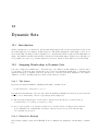
12 Dynamic Sets
12.1 Introduction . . . . . . . . . . . . . . . . . . . . . . . . . . .
12.2 Assigning Membership to Dynamic Sets . . . . . . . . . . .
12.2.1 The Syntax . . . . . . . . . . . . . . . . . . . . . . .
12.2.2 Illustrative Example . . . . . . . . . . . . . . . . . .
12.2.3 Dynamic Sets with Multiple Indices . . . . . . . . .
12.2.4 Assignments over the Domain of Dynamic Sets . . .
12.2.5 Equations Defined over the Domain of Dynamic Sets
12.2.6 Assigning Membership to Singleton Sets . . . . . . .
12.3 Using Dollar Controls with Dynamic Sets . . . . . . . . . . .
12.3.1 Assignments . . . . . . . . . . . . . . . . . . . . . .
12.3.2 Indexed Operations . . . . . . . . . . . . . . . . . .
12.3.3 Equations . . . . . . . . . . . . . . . . . . . . . . . .
12.3.4 Filtering through Dynamic Sets . . . . . . . . . . . .
12.4 Set Operations . . . . . . . . . . . . . . . . . . . . . . . . . .
12.4.1 Set Union . . . . . . . . . . . . . . . . . . . . . . . .
12.4.2 Set Intersection . . . . . . . . . . . . . . . . . . . . .
12.4.3 Set Complement . . . . . . . . . . . . . . . . . . . .
12.4.4 Set Difference . . . . . . . . . . . . . . . . . . . . . .
12.5 Summary . . . . . . . . . . . . . . . . . . . . . . . . . . . . .
13 Sets
13.1
13.2
13.3
13.4
13.5
13.6
13.7
.
.
.
.
.
.
.
.
.
.
.
.
.
.
.
.
.
.
.
.
.
.
.
.
.
.
.
.
.
.
.
.
.
.
.
.
.
.
.
.
.
.
.
.
.
.
.
.
.
.
.
.
.
.
.
.
.
.
.
.
.
.
.
.
.
.
.
.
.
.
.
.
.
.
.
.
.
.
.
.
.
.
.
.
.
.
.
.
.
.
.
.
.
.
.
.
.
.
.
.
.
.
.
.
.
.
.
.
.
.
.
.
.
.
.
.
.
.
.
.
.
.
.
.
.
.
.
.
.
.
.
.
.
.
.
.
.
.
.
.
.
.
.
.
.
.
.
.
.
.
.
.
.
.
.
.
.
.
.
.
.
.
.
.
.
.
.
.
.
.
.
.
.
.
.
.
.
.
.
.
.
.
.
.
.
.
.
.
.
.
.
.
.
.
.
.
.
.
.
.
.
.
.
.
.
.
.
.
.
.
.
.
.
.
.
.
.
.
.
.
.
.
.
.
.
.
.
.
.
.
.
.
.
.
.
.
.
.
.
.
.
.
.
.
.
.
.
.
.
.
.
.
.
.
.
.
.
.
.
.
.
.
.
.
.
.
.
.
.
.
.
.
.
.
.
.
.
.
.
.
.
.
.
.
.
.
.
.
.
.
.
.
.
.
.
.
.
.
.
.
.
.
.
.
.
.
.
.
.
.
.
.
.
.
.
.
.
.
.
.
.
.
.
.
.
.
.
.
.
.
.
.
.
.
.
.
.
.
.
.
.
.
.
.
.
.
.
.
.
.
.
.
.
.
.
.
.
.
.
.
.
.
.
.
.
.
.
.
.
.
.
.
.
.
.
.
.
.
.
.
119
119
119
119
119
120
120
121
121
121
122
122
122
123
123
123
123
123
124
124
.
.
.
.
.
.
.
.
.
.
.
.
.
.
.
.
.
.
.
.
.
.
.
.
.
.
.
.
.
.
.
.
.
.
.
.
.
.
.
.
.
.
.
.
.
.
.
.
.
.
.
.
.
.
.
.
.
.
.
.
.
.
.
.
.
.
.
.
.
.
.
.
.
.
.
.
.
.
.
.
.
.
.
.
.
.
.
.
.
.
.
.
.
.
.
.
.
.
.
.
.
.
.
.
.
.
.
.
.
.
.
.
.
.
.
.
.
.
.
.
.
.
.
.
.
.
.
.
.
.
.
.
.
.
.
.
.
.
.
.
.
.
.
.
.
.
.
.
.
.
.
.
.
.
.
.
.
.
.
.
.
.
.
.
.
.
.
.
.
.
.
.
.
.
.
.
.
.
.
.
.
.
.
.
.
.
.
.
.
.
.
.
.
.
.
.
.
.
.
.
.
.
.
.
.
.
.
.
.
.
.
.
.
.
.
.
.
.
.
.
.
.
.
.
.
.
.
.
.
.
.
.
.
.
.
.
.
.
.
.
.
.
.
.
.
.
.
.
.
.
.
.
.
.
.
.
.
.
.
.
.
.
.
.
.
.
.
.
.
.
.
.
.
.
.
.
.
.
.
.
.
.
.
.
.
.
.
.
.
.
.
.
.
.
.
.
.
.
.
.
.
.
.
.
.
.
.
.
.
.
.
.
.
.
.
.
.
.
.
.
.
.
.
.
.
.
.
.
.
.
125
125
125
126
126
127
127
127
128
128
129
129
130
130
131
131
. . . .
. . . .
. . . .
. . . .
. . . .
. . . .
. . . .
. . . .
in List
. . . . .
. . . . .
. . . . .
. . . . .
. . . . .
. . . . .
. . . . .
. . . . .
Format
.
.
.
.
.
.
.
.
.
.
.
.
.
.
.
.
.
.
.
.
.
.
.
.
.
.
.
.
.
.
.
.
.
.
.
.
.
.
.
.
.
.
.
.
.
.
.
.
.
.
.
.
.
.
.
.
.
.
.
.
.
.
.
.
.
.
.
.
.
.
.
.
.
.
.
.
.
.
.
.
.
.
.
.
.
.
.
.
.
.
.
.
.
.
.
.
.
.
.
.
.
.
.
.
.
.
.
.
.
.
.
.
.
.
.
.
.
.
.
.
.
.
.
.
.
.
.
.
.
.
.
.
.
.
.
.
.
.
.
.
.
.
.
.
.
.
.
.
.
.
.
.
.
.
.
.
.
.
.
.
.
.
.
.
.
.
.
.
.
.
.
.
.
.
.
.
.
.
.
.
.
.
.
.
.
.
.
.
.
133
133
133
133
134
135
135
136
136
137
.
.
.
.
.
.
.
.
.
.
.
.
.
.
.
.
.
.
.
.
.
.
.
.
.
.
.
.
.
.
.
.
.
.
.
.
.
.
.
.
.
.
.
.
.
.
.
.
.
.
.
.
.
.
.
.
.
.
.
.
.
.
.
.
.
.
.
.
.
.
.
.
.
.
.
.
.
.
.
.
.
.
.
.
.
.
.
.
.
.
.
.
.
.
.
.
.
.
.
.
.
.
.
.
.
.
.
.
.
.
.
.
.
.
.
139
139
139
140
141
141
as Sequences: Ordered Sets
Introduction . . . . . . . . . . . . . . . . . . . . . . . . . .
Ordered and Unordered Sets . . . . . . . . . . . . . . . . .
Ord and Card . . . . . . . . . . . . . . . . . . . . . . . . .
13.3.1 The Ord Operator . . . . . . . . . . . . . . . . . .
13.3.2 The Card Operator . . . . . . . . . . . . . . . . .
Lag and Lead Operators . . . . . . . . . . . . . . . . . . .
Lags and Leads in Assignments . . . . . . . . . . . . . . .
13.5.1 Linear Lag and Lead Operators - Reference . . . .
13.5.2 Linear Lag and Lead Operators - Assignment . . .
13.5.3 Circular Lag and Lead Operators . . . . . . . . . .
Lags and Leads in Equations . . . . . . . . . . . . . . . . .
13.6.1 Linear Lag and Lead Operators - Domain Control
13.6.2 Linear Lag and Lead Operators - Reference . . . .
13.6.3 Circular Lag and Lead Operators . . . . . . . . . .
Summary . . . . . . . . . . . . . . . . . . . . . . . . . . . .
14 The
14.1
14.2
14.3
14.4
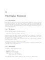
Display Statement
Introduction . . . . . . . . . . . . . . . . . .
The Syntax . . . . . . . . . . . . . . . . . .
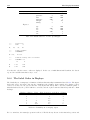
An Example . . . . . . . . . . . . . . . . . .
The Label Order in Displays . . . . . . . . .
14.4.1 Example . . . . . . . . . . . . . . . .
14.5 Display Controls . . . . . . . . . . . . . . . .
14.5.1 Global Display Controls . . . . . . .
14.5.2 Local Display Control . . . . . . . .
14.5.3 Display Statement to Generate Data
15 The
15.1
15.2
15.3
15.4
.
.
.
.
.
.
.
.
.
.
.
.
.
.
.
.
.
.
.
Put Writing Facility
Introduction . . . . . .
The Syntax . . . . . .
An Example . . . . . .
Output Files . . . . . .
15.4.1 Defining Files .
.
.
.
.
.
.
.
.
.
.
.
.
.
.
.
.
.
.
.
.
.
.
.
.
.
.
.
.
.
.
.
.
.
.
.
.
.
.
.
.
.
.
.
.
.
.
.
.
.
.
.
.
.
.
.
.
.
.
.
.
.
.
.
.
.
.
.
.
.
.
.
.
.
.
.
.
.
.
.
.
.
.
.
.
.
.
.
.
.
.
.
.
.
.
.
8
TABLE OF CONTENTS
15.5
15.6
15.7
15.8
15.9
15.10
15.11
15.12
15.13
15.14
15.15
15.16
15.17
15.4.2 Assigning Files . . . . . . . . . . . . . . . . .
15.4.3 Closing a File . . . . . . . . . . . . . . . . . .
15.4.4 Appending to a File . . . . . . . . . . . . . .
Page Format . . . . . . . . . . . . . . . . . . . . . . .
Page Sections . . . . . . . . . . . . . . . . . . . . . .
15.6.1 Accessing Various Page Sections . . . . . . .
15.6.2 Paging . . . . . . . . . . . . . . . . . . . . . .
Positioning the Cursor on a Page . . . . . . . . . . .
System Suffixes . . . . . . . . . . . . . . . . . . . . .
Output Items . . . . . . . . . . . . . . . . . . . . . .
15.9.1 Text Items . . . . . . . . . . . . . . . . . . .
15.9.2 Numeric Items . . . . . . . . . . . . . . . . .
15.9.3 Set Value Items . . . . . . . . . . . . . . . . .
Global Item Formatting . . . . . . . . . . . . . . . .
15.10.1 Field Justification . . . . . . . . . . . . . . .
15.10.2 Field Width . . . . . . . . . . . . . . . . . . .
Local Item Formatting . . . . . . . . . . . . . . . . .
Additional Numeric Display Control . . . . . . . . . .
15.12.1 Illustrative Example . . . . . . . . . . . . . .
Cursor Control . . . . . . . . . . . . . . . . . . . . .
15.13.1 Current Cursor Column . . . . . . . . . . . .
15.13.2 Current Cursor Row . . . . . . . . . . . . . .
15.13.3 Last Line Control . . . . . . . . . . . . . . .
Paging Control . . . . . . . . . . . . . . . . . . . . .
Exception Handling . . . . . . . . . . . . . . . . . . .
Source of Errors Associated with the Put Statement .
15.16.1 Syntax Errors . . . . . . . . . . . . . . . . . .
15.16.2 Put Errors . . . . . . . . . . . . . . . . . . .
Simple Spreadsheet/Database Application . . . . . .
15.17.1 An Example . . . . . . . . . . . . . . . . . .
16 Programming Flow Control Features
16.1 Introduction . . . . . . . . . . . . .
16.2 The Loop Statement . . . . . . . .
16.2.1 The Syntax . . . . . . . . .
16.2.2 Examples . . . . . . . . . .
16.3 The If-Elseif-Else Statement . . . .
16.3.1 The Syntax . . . . . . . . .
16.3.2 Examples . . . . . . . . . .
16.4 The While Statement . . . . . . . .
16.4.1 The Syntax . . . . . . . . .
16.4.2 Examples . . . . . . . . . .
16.5 The For Statement . . . . . . . . .
16.5.1 The Syntax . . . . . . . . .
16.5.2 Examples . . . . . . . . . .
.
.
.
.
.
.
.
.
.
.
.
.
.
.
.
.
.
.
.
.
.
.
.
.
.
.
.
.
.
.
.
.
.
.
.
.
.
.
.
.
.
.
.
.
.
.
.
.
.
.
.
.
.
.
.
.
.
.
.
.
.
.
.
.
.
.
.
.
.
.
.
.
.
.
.
.
.
.
.
.
.
.
.
.
.
.
.
.
.
.
.
.
.
.
.
.
.
.
.
.
.
.
.
.
.
.
.
.
.
.
.
.
.
.
.
.
.
.
.
.
.
.
.
.
.
.
.
.
.
.
.
.
.
.
.
.
.
.
.
.
.
.
.
.
.
.
.
.
.
.
.
.
.
.
.
.
.
.
.
.
.
.
.
.
.
.
.
.
.
.
.
.
.
.
.
.
.
.
.
.
.
.
.
.
.
.
.
.
.
.
.
.
.
.
.
.
.
.
.
.
.
.
.
.
.
.
.
.
.
.
.
.
.
.
.
.
.
.
.
.
.
.
.
.
.
.
.
.
.
.
.
.
.
.
.
.
.
.
.
.
.
.
.
.
.
.
.
.
.
.
.
.
.
.
.
.
.
.
.
.
.
.
.
.
.
.
.
.
.
.
.
.
.
.
.
.
.
.
.
.
.
.
.
.
.
.
.
.
.
.
.
.
.
.
.
.
.
.
.
.
.
.
.
.
.
.
.
.
.
.
.
.
.
.
.
.
.
.
.
.
.
.
.
.
.
.
.
.
.
.
.
.
.
.
.
.
.
.
.
.
.
.
.
.
.
.
.
.
.
.
.
.
.
.
.
.
.
.
.
.
.
.
.
.
.
.
.
.
.
.
.
.
.
.
.
.
.
.
.
.
.
.
.
.
.
.
.
.
.
.
.
.
.
.
.
.
.
.
.
.
.
.
.
.
.
.
.
.
.
.
.
.
.
.
.
.
.
.
.
.
.
.
.
.
.
.
.
.
.
.
.
.
.
.
.
.
.
.
.
.
.
.
.
.
.
.
.
.
.
.
.
.
.
.
.
.
.
.
.
.
.
.
.
.
.
.
.
.
.
.
.
.
.
.
.
.
.
.
.
.
.
.
.
.
.
.
.
.
.
.
.
.
.
.
.
.
.
.
.
.
.
.
.
.
.
.
.
.
.
.
.
.
.
.
.
.
.
.
.
.
.
.
.
.
.
.
.
.
.
.
.
.
.
.
.
.
.
.
.
.
.
.
.
.
.
.
.
.
.
.
.
.
.
.
.
.
.
.
.
.
.
.
.
.
.
.
.
.
.
.
.
.
.
.
.
.
.
.
.
.
.
.
.
.
.
.
.
.
.
.
.
.
.
.
.
.
.
.
.
.
.
.
.
.
.
.
.
.
.
.
.
.
.
.
.
.
.
.
.
.
.
.
.
.
.
.
.
.
.
.
.
.
.
.
.
.
.
.
.
.
.
.
.
.
.
.
.
.
.
.
.
.
.
.
.
.
.
.
.
.
.
.
.
.
.
.
.
.
.
.
.
.
.
.
.
.
.
.
.
.
.
.
.
.
.
.
.
.
.
.
.
.
.
.
.
.
.
.
.
.
.
.
.
.
.
.
.
.
.
.
.
.
.
.
.
.
.
.
.
.
.
.
.
.
.
.
.
.
.
.
.
.
.
.
.
.
.
.
.
.
.
.
.
.
.
.
.
.
.
.
141
142
142
142
143
144
144
144
145
145
146
147
147
147
147
148
148
149
149
150
150
151
151
152
152
152
152
152
153
153
.
.
.
.
.
.
.
.
.
.
.
.
.
.
.
.
.
.
.
.
.
.
.
.
.
.
.
.
.
.
.
.
.
.
.
.
.
.
.
.
.
.
.
.
.
.
.
.
.
.
.
.
.
.
.
.
.
.
.
.
.
.
.
.
.
.
.
.
.
.
.
.
.
.
.
.
.
.
.
.
.
.
.
.
.
.
.
.
.
.
.
.
.
.
.
.
.
.
.
.
.
.
.
.
.
.
.
.
.
.
.
.
.
.
.
.
.
.
.
.
.
.
.
.
.
.
.
.
.
.
.
.
.
.
.
.
.
.
.
.
.
.
.
.
.
.
.
.
.
.
.
.
.
.
.
.
.
.
.
.
.
.
.
.
.
.
.
.
.
.
.
.
.
.
.
.
.
.
.
.
.
.
.
.
.
.
.
.
.
.
.
.
.
.
.
.
.
.
.
.
.
.
.
.
.
.
.
.
.
.
.
.
.
.
.
.
.
.
.
.
.
.
.
.
.
.
.
.
.
.
.
.
.
.
.
.
.
.
.
.
.
.
.
.
.
.
.
.
.
.
.
.
.
.
.
.
.
.
.
.
.
.
.
.
.
.
.
.
.
.
.
.
.
.
.
.
.
.
.
.
.
.
.
.
.
.
.
.
.
.
.
.
.
.
.
.
.
.
.
.
.
.
.
.
.
.
.
.
.
.
.
.
.
.
.
.
.
.
.
.
.
.
.
.
.
.
.
.
.
.
.
.
.
.
.
.
.
.
.
.
.
.
.
.
.
.
.
.
.
.
.
.
.
.
.
.
.
.
.
.
.
.
.
.
.
.
.
.
.
.
.
.
.
.
.
.
.
.
.
.
.
.
.
.
.
.
.
.
.
.
.
.
.
.
.
.
.
.
.
.
.
.
.
155
155
155
155
156
156
156
157
158
158
158
158
159
159
17 Special Language Features
17.1 Introduction . . . . . . . . . . . . . . . . . .
17.2 Special MIP Features . . . . . . . . . . . . .
17.2.1 Types of Discrete Variables . . . . .
17.2.2 Special Order Sets of Type 1 (SOS1)
17.2.3 Special Order Sets of Type 2 (SOS2)
17.2.4 Semi-Continuous Variables . . . . .
17.2.5 Semi-Integer Variables . . . . . . . .
17.2.6 Setting Priorities for Branching . . .
17.3 Model Scaling - The Scale Option . . . . . .
.
.
.
.
.
.
.
.
.
.
.
.
.
.
.
.
.
.
.
.
.
.
.
.
.
.
.
.
.
.
.
.
.
.
.
.
.
.
.
.
.
.
.
.
.
.
.
.
.
.
.
.
.
.
.
.
.
.
.
.
.
.
.
.
.
.
.
.
.
.
.
.
.
.
.
.
.
.
.
.
.
.
.
.
.
.
.
.
.
.
.
.
.
.
.
.
.
.
.
.
.
.
.
.
.
.
.
.
.
.
.
.
.
.
.
.
.
.
.
.
.
.
.
.
.
.
.
.
.
.
.
.
.
.
.
.
.
.
.
.
.
.
.
.
.
.
.
.
.
.
.
.
.
.
.
.
.
.
.
.
.
.
.
.
.
.
.
.
.
.
.
.
.
.
.
.
.
.
.
.
.
.
.
.
.
.
.
.
.
.
.
.
.
.
.
.
.
.
.
.
.
.
.
.
.
.
.
.
.
.
.
.
.
.
.
.
.
.
.
.
.
.
.
.
.
.
.
.
.
.
.
.
.
.
.
.
.
.
.
.
.
.
.
.
.
.
.
.
.
.
.
.
.
.
.
.
.
.
.
.
.
.
.
.
.
.
.
.
.
.
161
161
161
161
161
162
163
163
164
164
.
.
.
.
.
.
.
.
.
.
.
.
.
.
.
.
.
.
.
.
.
.
.
.
.
.
.
.
.
.
.
.
.
.
.
.
.
.
.
.
.
.
.
.
.
.
.
.
.
.
.
.
TABLE OF CONTENTS
17.3.1
17.3.2
17.3.3
17.3.4
The Scale Option . . .
Variable Scaling . . .
Equation Scaling . . .
Scaling of Derivatives
9
.
.
.
.
.
.
.
.
.
.
.
.
.
.
.
.
.
.
.
.
.
.
.
.
.
.
.
.
.
.
.
.
.
.
.
.
.
.
.
.
.
.
.
.
.
.
.
.
.
.
.
.
.
.
.
.
.
.
.
.
.
.
.
.
.
.
.
.
.
.
.
.
.
.
.
.
.
.
.
.
.
.
.
.
.
.
.
.
.
.
.
.
.
.
.
.
.
.
.
.
.
.
.
.
.
.
.
.
.
.
.
.
.
.
.
.
.
.
.
.
.
.
.
.
.
.
.
.
.
.
.
.
.
.
.
.
.
.
.
.
.
.
.
.
.
.
.
.
.
.
.
.
164
165
165
166
Appendix
168
A Glossary
169
B The GAMS Model Library
175
C The GAMS Call
C.1 The Generic “no frills” GAMS Call . . . . . . . . . . .
C.1.1 Specifying Options through the Command Line
C.2 List of Command Line Parameters . . . . . . . . . . .
C.3 Detailed Description of Command Line Parameters . .
.
.
.
.
.
.
.
.
.
.
.
.
.
.
.
.
.
.
.
.
.
.
.
.
.
.
.
.
.
.
.
.
.
.
.
.
.
.
.
.
.
.
.
.
.
.
.
.
.
.
.
.
.
.
.
.
.
.
.
.
.
.
.
.
.
.
.
.
.
.
.
.
.
.
.
.
.
.
.
.
.
.
.
.
.
.
.
.
.
.
.
.
.
.
.
.
177
177
177
178
179
D Dollar Control Options
D.1 Introduction . . . . . . . . . . . . . . . . . . . .
D.1.1 Syntax . . . . . . . . . . . . . . . . . . .
D.2 List of Dollar Control Options . . . . . . . . . .
D.3 Detailed Description of Dollar Control Options
.
.
.
.
.
.
.
.
.
.
.
.
.
.
.
.
.
.
.
.
.
.
.
.
.
.
.
.
.
.
.
.
.
.
.
.
.
.
.
.
.
.
.
.
.
.
.
.
.
.
.
.
.
.
.
.
.
.
.
.
.
.
.
.
.
.
.
.
.
.
.
.
.
.
.
.
.
.
.
.
.
.
.
.
.
.
.
.
.
.
.
.
.
.
.
.
.
.
.
.
.
.
.
.
.
.
.
.
.
.
.
.
203
203
203
203
206
E The Option Statement
E.1 Introduction . . . . . . . . . . .
E.1.1 The Syntax . . . . . . .
E.2 List of Options . . . . . . . . .
E.3 Detailed Description of Options
.
.
.
.
.
.
.
.
.
.
.
.
.
.
.
.
.
.
.
.
.
.
.
.
.
.
.
.
.
.
.
.
.
.
.
.
.
.
.
.
.
.
.
.
.
.
.
.
.
.
.
.
.
.
.
.
.
.
.
.
.
.
.
.
.
.
.
.
.
.
.
.
.
.
.
.
.
.
.
.
.
.
.
.
.
.
.
.
.
.
.
.
.
.
.
.
.
.
.
.
.
.
.
.
.
.
.
.
.
.
.
.
.
.
.
.
.
.
.
.
.
.
.
.
245
245
245
246
247
F The Save and Restart Feature
F.1 Introduction . . . . . . . . . . . . . . . . . .
F.2 The Save and Restart Feature . . . . . . . .
F.2.1 Saving The Work File . . . . . . . .
F.2.2 Restarting from the Work File . . .
F.3 Ways in which a Work File is Useful . . . .
F.3.1 Separation of Model and Data . . .
F.3.2 Incremental Program Development .
F.3.3 Tacking Sequences of Difficult Solves
F.3.4 Multiple Scenarios . . . . . . . . . .
F.3.5 The GAMS Runtime License . . . .
.
.
.
.
.
.
.
.
.
.
.
.
.
.
.
.
.
.
.
.
.
.
.
.
.
.
.
.
.
.
.
.
.
.
.
.
.
.
.
.
.
.
.
.
.
.
.
.
.
.
.
.
.
.
.
.
.
.
.
.
.
.
.
.
.
.
.
.
.
.
.
.
.
.
.
.
.
.
.
.
.
.
.
.
.
.
.
.
.
.
.
.
.
.
.
.
.
.
.
.
.
.
.
.
.
.
.
.
.
.
.
.
.
.
.
.
.
.
.
.
.
.
.
.
.
.
.
.
.
.
.
.
.
.
.
.
.
.
.
.
.
.
.
.
.
.
.
.
.
.
.
.
.
.
.
.
.
.
.
.
.
.
.
.
.
.
.
.
.
.
.
.
.
.
.
.
.
.
.
.
.
.
.
.
.
.
.
.
.
.
.
.
.
.
.
.
.
.
.
.
.
.
.
.
.
.
.
.
.
.
.
.
.
.
.
.
.
.
.
.
.
.
.
.
.
.
.
.
.
.
.
.
.
.
.
.
.
.
.
.
.
.
.
.
.
.
.
.
.
.
.
.
.
.
.
.
.
.
.
.
.
.
.
.
.
.
.
.
.
.
.
.
.
.
.
.
.
.
.
.
.
.
.
.
.
.
.
.
.
.
.
.
.
.
.
.
.
.
.
.
251
251
251
252
252
253
253
254
255
255
255
G Secure Work Files
G.1 Introduction . . . . . . . . . . . . . .
G.2 A First Example . . . . . . . . . . . .
G.3 Secure Work Files . . . . . . . . . . .
G.4 Access Control Commands . . . . . .
G.5 Advanced Use of Access Control . . .
G.6 Limitations and Future Requirements
G.7 Obfuscated Work Files . . . . . . . .
.
.
.
.
.
.
.
.
.
.
.
.
.
.
.
.
.
.
.
.
.
.
.
.
.
.
.
.
.
.
.
.
.
.
.
.
.
.
.
.
.
.
.
.
.
.
.
.
.
.
.
.
.
.
.
.
.
.
.
.
.
.
.
.
.
.
.
.
.
.
.
.
.
.
.
.
.
.
.
.
.
.
.
.
.
.
.
.
.
.
.
.
.
.
.
.
.
.
.
.
.
.
.
.
.
.
.
.
.
.
.
.
.
.
.
.
.
.
.
.
.
.
.
.
.
.
.
.
.
.
.
.
.
.
.
.
.
.
.
.
.
.
.
.
.
.
.
.
.
.
.
.
.
.
.
.
.
.
.
.
.
.
.
.
.
.
.
.
.
.
.
.
.
.
.
.
.
.
.
.
.
.
.
.
.
.
.
.
.
.
.
.
.
.
.
.
.
.
.
.
.
.
.
.
.
.
.
.
.
.
.
.
.
.
.
.
.
.
.
.
.
.
.
.
.
.
.
.
.
.
.
.
.
.
.
.
.
.
.
.
.
.
.
.
.
.
.
.
.
.
.
.
.
.
.
.
.
.
.
.
.
.
257
257
258
259
259
260
261
262
H Compressed and Encrypted Input Files
H.1 Introduction . . . . . . . . . . . . . . .
H.2 A First Example . . . . . . . . . . . . .
H.3 The CEFILES Gamslib Model . . . . .
H.4 The ENCRYPT GAMSLIB Model . . .
.
.
.
.
.
.
.
.
.
.
.
.
.
.
.
.
.
.
.
.
.
.
.
.
.
.
.
.
.
.
.
.
.
.
.
.
.
.
.
.
.
.
.
.
.
.
.
.
.
.
.
.
.
.
.
.
.
.
.
.
.
.
.
.
.
.
.
.
.
.
.
.
.
.
.
.
.
.
.
.
.
.
.
.
.
.
.
.
.
.
.
.
.
.
.
.
.
.
.
.
.
.
.
.
.
.
.
.
.
.
.
.
.
.
.
.
.
.
.
.
.
.
.
.
.
.
.
.
.
.
.
.
265
265
265
266
267
I
The GAMS Grid Computing Facility
269
I.1
Introduction . . . . . . . . . . . . . . . . . . . . . . . . . . . . . . . . . . . . . . . . . . . . . . . . 269
10
TABLE OF CONTENTS
I.2
I.3
I.4
.
.
.
.
.
.
.
.
.
.
.
.
.
.
.
.
.
.
.
.
.
.
.
.
.
.
.
.
.
.
.
.
.
.
.
.
.
.
.
.
.
.
.
.
.
.
.
.
.
.
.
.
.
.
.
.
.
.
.
.
.
.
.
.
.
.
.
.
.
.
.
.
.
.
.
.
.
.
.
.
.
.
.
.
.
.
.
.
.
.
.
.
.
.
.
.
.
.
.
.
.
.
.
.
.
.
.
.
.
.
.
.
.
.
.
.
.
.
.
.
.
.
.
.
.
.
.
.
.
.
.
.
.
.
.
.
.
.
.
.
.
.
.
.
.
.
.
.
.
.
.
.
.
.
.
.
.
.
.
.
.
.
.
.
.
.
.
.
.
.
.
.
.
.
.
.
.
.
.
.
.
.
.
.
.
.
.
.
.
.
.
.
.
.
.
.
.
.
.
.
.
.
.
.
269
270
272
272
273
274
274
275
275
275
276
277
J Extrinsic Functions
J.1
Introduction . . . . . . . . . . . . . . . . . . . . . . .
J.2
Fitpack Library . . . . . . . . . . . . . . . . . . . . .
J.3
Piecewise Polynomial Library . . . . . . . . . . . . .
J.4
Stochastic Library . . . . . . . . . . . . . . . . . . . .
J.5
LINDO Sampling Library . . . . . . . . . . . . . . .
J.6
Build Your Own: Trigonometric Library Example . .
J.7
Build Your Own: Reading the GAMS Parameter File
J.8
CPP Library . . . . . . . . . . . . . . . . . . . . . . .
J.8.1
Automatic differentiation . . . . . . . . . . .
J.8.2
Multi-variate Normal Distributions . . . . . .
. . . . . . . . .
. . . . . . . . .
. . . . . . . . .
. . . . . . . . .
. . . . . . . . .
. . . . . . . . .
in your Library
. . . . . . . . .
. . . . . . . . .
. . . . . . . . .
.
.
.
.
.
.
.
.
.
.
.
.
.
.
.
.
.
.
.
.
.
.
.
.
.
.
.
.
.
.
.
.
.
.
.
.
.
.
.
.
.
.
.
.
.
.
.
.
.
.
.
.
.
.
.
.
.
.
.
.
.
.
.
.
.
.
.
.
.
.
.
.
.
.
.
.
.
.
.
.
.
.
.
.
.
.
.
.
.
.
.
.
.
.
.
.
.
.
.
.
.
.
.
.
.
.
.
.
.
.
.
.
.
.
.
.
.
.
.
.
.
.
.
.
.
.
.
.
.
.
.
.
.
.
.
.
.
.
.
.
.
.
.
.
.
.
.
.
.
.
.
.
.
.
.
.
.
.
.
.
279
279
279
280
281
283
286
287
288
288
288
K Installation and System Notes
K.1 Installation . . . . . . . . . . .
K.2 Command Line Use of GAMS
K.3 Installation . . . . . . . . . . .
K.4 Access to GAMS . . . . . . .
K.5 Installation . . . . . . . . . . .
K.6 Access to GAMS . . . . . . .
K.7 Example . . . . . . . . . . . .
.
.
.
.
.
.
.
.
.
.
.
.
.
.
.
.
.
.
.
.
.
.
.
.
.
.
.
.
.
.
.
.
.
.
.
.
.
.
.
.
.
.
.
.
.
.
.
.
.
.
.
.
.
.
.
.
.
.
.
.
.
.
.
.
.
.
.
.
.
.
.
.
.
.
.
.
.
.
.
.
.
.
.
.
.
.
.
.
.
.
.
.
.
.
.
.
.
.
.
.
.
.
.
.
.
.
.
.
.
.
.
.
.
.
.
.
.
.
.
291
291
292
292
293
294
295
295
I.5
I.6
I.7
Index
Basic Concepts . . . . . . . . . .
A First Example . . . . . . . . . .
Advanced use of Grid Features . .
I.4.1
Very Long Job Durations
Summary of Grid Features . . . .
I.5.1
Grid Handle Functions . .
I.5.2
Grid Model Attributes . .
I.5.3
Grid Solution Retrieval .
I.5.4
Grid Directory . . . . . .
Architecture and Customization .
I.6.1
Grid Submission Testing .
Glossary and Definitions . . . . .
.
.
.
.
.
.
.
.
.
.
.
.
.
.
.
.
.
.
.
.
.
.
.
.
.
.
.
.
.
.
.
.
.
.
.
.
.
.
.
.
.
.
.
.
.
.
.
.
.
.
.
.
.
.
.
.
.
.
.
.
.
.
.
.
.
.
.
.
.
.
.
.
.
.
.
.
.
.
.
.
.
.
.
.
.
.
.
.
.
.
.
.
.
.
.
.
.
.
.
.
.
.
.
.
.
.
.
.
.
.
.
.
.
.
.
.
.
.
.
.
.
.
.
.
.
.
.
.
.
.
.
.
.
.
.
.
.
.
.
.
.
.
.
.
.
.
.
.
.
.
.
.
.
.
.
.
.
.
.
.
.
.
.
.
.
.
.
.
.
.
.
.
.
.
.
.
.
.
.
.
.
.
.
.
.
.
.
.
.
.
.
.
.
.
.
.
.
.
.
.
.
.
.
.
.
.
.
.
.
.
.
.
.
.
.
.
.
.
.
.
.
.
.
.
.
.
.
.
.
.
.
.
.
.
.
.
.
.
.
.
.
.
.
.
.
.
.
.
.
.
.
.
.
.
.
.
.
.
.
.
.
.
.
.
.
.
.
.
.
.
.
.
.
.
.
.
.
.
.
.
.
.
.
.
.
.
.
.
.
.
.
.
.
.
.
.
.
.
.
.
.
.
.
.
.
.
.
.
.
.
.
.
.
.
.
.
.
.
.
.
.
.
.
.
.
.
.
.
.
.
.
.
.
.
.
.
.
.
.
.
.
.
.
.
.
.
.
.
.
.
.
.
.
.
.
.
.
.
.
.
.
.
.
.
.
.
.
.
.
.
.
.
.
.
.
299
List of Tables
2.1
2.2
2.3
Data for the transportation problem (adapted from Dantzig, 1963) . . . . . . . . . . . . . . . . . . 6
The basic components of a GAMS model . . . . . . . . . . . . . . . . . . . . . . . . . . . . . . . . 8
Permissible variable types . . . . . . . . . . . . . . . . . . . . . . . . . . . . . . . . . . . . . . . . . 12
3.1
3.2
3.3
3.4
Organization of GAMS programs . .
Legal characters . . . . . . . . . . .
Reserved words and symbols . . . .
Rules for constructing identifiers and
4.1
Examples of the compact representation of sets . . . . . . . . . . . . . . . . . . . . . . . . . . . . . 41
6.1
6.2
6.3
GAMS functions . . . . . . . . . . . . . . . . . . . . . . . . . . . . . . . . . . . . . . . . . . . . . . 63
Special symbols for extended arithmetic . . . . . . . . . . . . . . . . . . . . . . . . . . . . . . . . . 65
Exponentiation and Division . . . . . . . . . . . . . . . . . . . . . . . . . . . . . . . . . . . . . . . 66
7.1
Variable types and default bounds . . . . . . . . . . . . . . . . . . . . . . . . . . . . . . . . . . . . 68
8.1
8.2
Classification of functions with endogenous arguments . . . . . . . . . . . . . . . . . . . . . . . . . 76
Subfield definitions for equations . . . . . . . . . . . . . . . . . . . . . . . . . . . . . . . . . . . . 77
9.1
9.2
Model Attributes mainly used before solve . . . . . . . . . . . . . . . . . . . . . . . . . . . . . . . . 84
Model Attributes mainly used after solve . . . . . . . . . . . . . . . . . . . . . . . . . . . . . . . . . 85
. . . .
. . . .
. . . .
labels
.
.
.
.
.
.
.
.
.
.
.
.
.
.
.
.
.
.
.
.
.
.
.
.
.
.
.
.
.
.
.
.
.
.
.
.
.
.
.
.
.
.
.
.
.
.
.
.
.
.
.
.
.
.
.
.
.
.
.
.
.
.
.
.
.
.
.
.
.
.
.
.
.
.
.
.
.
.
.
.
.
.
.
.
.
.
.
.
.
.
.
.
.
.
.
.
.
.
.
.
.
.
.
.
.
.
.
.
.
.
.
.
.
.
.
.
.
.
.
.
.
.
.
.
29
30
30
31
10.1 List of GAMS data types . . . . . . . . . . . . . . . . . . . . . . . . . . . . . . . . . . . . . . . . . 94
11.1 Truth table of logical operators . . . . . . . . . . . . . . . . . . . . . . . . . . . . . . . . . . . . . . 110
11.2 Operator precedence . . . . . . . . . . . . . . . . . . . . . . . . . . . . . . . . . . . . . . . . . . . . 111
11.3 Examples of logical conditions . . . . . . . . . . . . . . . . . . . . . . . . . . . . . . . . . . . . . . . 112
14.1 Default values for .lo and .up subtypes . . . . . . . . . . . . . . . . . . . . . . . . . . . . . . . . 134
14.2 Default layout of display output . . . . . . . . . . . . . . . . . . . . . . . . . . . . . . . . . . . . . 134
C.1 GAMS command line parameters . . . . . . . . . . . . . . . . . . . . . . . . . . . . . . . . . . . . . 179
D.1 Dollar control options . . . . . . . . . . . . . . . . . . . . . . . . . . . . . . . . . . . . . . . . . . . 205
E.1 GAMS options . . . . . . . . . . . . . . . . . . . . . . . . . . . . . . . . . . . . . . . . . . . . . . . 246
J.1
J.2
J.3
J.4
J.5
J.6
J.7
J.8
Fitpack functions . . . . . . . .
Piecewise polynomial functions
Random number generators . .
Distribution functions . . . . .
Normal distribution functions .
LINDO sampling functions . .
Trigonometric functions . . . .
GAMS Parameter File reading
.
.
.
.
.
.
.
.
.
.
.
.
.
.
.
.
.
.
.
.
.
.
.
.
.
.
.
.
.
.
.
.
.
.
.
.
.
.
.
.
.
.
.
.
.
.
.
.
.
.
.
.
.
.
.
.
.
.
.
.
.
.
.
.
.
.
.
.
.
.
.
.
.
.
.
.
.
.
.
.
.
.
.
.
.
.
.
.
.
.
.
.
.
.
.
.
.
.
.
.
.
.
.
.
.
.
.
.
.
.
.
.
.
.
.
.
.
.
.
.
.
.
.
.
.
.
.
.
.
.
.
.
.
.
.
.
.
.
.
.
.
.
.
.
.
.
.
.
.
.
.
.
.
.
.
.
.
.
.
.
.
.
.
.
.
.
.
.
.
.
.
.
.
.
.
.
.
.
.
.
.
.
.
.
.
.
.
.
.
.
.
.
.
.
.
.
.
.
.
.
.
.
.
.
.
.
.
.
.
.
.
.
.
.
.
.
.
.
.
.
.
.
.
.
.
.
.
.
.
.
.
.
.
.
.
.
.
.
.
.
.
.
.
.
.
.
.
.
.
.
.
.
.
.
.
.
.
.
.
.
.
.
.
.
.
.
.
.
.
.
.
.
.
.
.
.
.
.
.
.
.
.
.
.
.
.
.
.
.
.
.
.
.
.
.
.
.
.
.
.
.
.
.
.
279
280
282
282
283
285
286
287
12
LIST OF TABLES
J.9
CPP Library functions . . . . . . . . . . . . . . . . . . . . . . . . . . . . . . . . . . . . . . . . . . . 288
1
Introduction
1.1
Motivation
Substantial progress was made in the 1950s and 1960s with the development of algorithms and computer codes
to solve large mathematical programming problems. The number of applications of these tools in the 1970s was
less then expected, however, because the solution procedures formed only a small part of the overall modeling
effort. A large part of the time required to develop a model involved data preparation and transformation and
report preparation. Each model required many hours of analyst and programming time to organize the data
and write the programs that would transform the data into the form required by the mathematical programming
optimizers. Furthermore, it was difficult to detect and eliminate errors because the programs that performed the
data operations were only accessible to the specialist who wrote them and not to the analysts in charge of the
project.
GAMS was developed to improve on this situation by:
â Providing a high-level language for the compact representation of large and complex models
â Allowing changes to be made in model specifications simply and safely
â Allowing unambiguous statements of algebraic relationships
â Permitting model descriptions that are independent of solution algorithms
1.2
1.2.1
Basic Features of GAMS
General Principles
The design of GAMS has incorporated ideas drawn from relational database theory and mathematical programming and has attempted to merge these ideas to suit the needs of strategic modelers. Relational database theory
provides a structured framework for developing general data organization and transformation capabilities. Mathematical programming provides a way of describing a problem and a variety of methods for solving it. The
following principles were used in designing the system:
1. All existing algorithmic methods should be available without changing the user’s model representation.
Introduction of new methods, or of new implementations of existing methods, should be possible
without requiring changes in existing models. Linear, nonlinear, mixed integer, mixed integer nonlinear
optimizations and mixed complementarity problems can currently be accommodated.
2. The optimization problem should be expressible independently of the data it uses. This separation of
logic and data allows a problem to be increased in size without causing an increase in the complexity of
the representation.
2
Introduction
3. The use of the relational data model requires that the allocation of computer resources be automated.
This means that large and complex models can be constructed without the user having to worry about
details such as array sizes and scratch storage.
1.2.2
Documentation
The GAMS model representation is in a form that can be easily read by people and by computers. This means
that the GAMS program itself is the documentation of the model, and that the separate description required in
the past (which was a burden to maintain, and which was seldom up-to-date) is no longer needed. Moreover, the
design of GAMS incorporates the following features that specifically address the user’s documentation needs:
â A GAMS model representation is concise, and makes full use of the elegance of the mathematical
representation.
â All data transformations are specified concisely and algebraically. This means that all data can be
entered in their most elemental form and that all transformations made in constructing the model and
in reporting are available for inspection.
â Explanatory text can be made part of the definition of all symbols and is reproduced whenever
associated values are displayed.
â All information needed to understand the model is in one document.
Of course some discipline is needed to take full advantage of these design features, but the aim is to make models
more accessible, more understandable, more verifiable, and hence more credible.
1.2.3
Portability
The GAMS system is designed so that models can be solved on different types of computers with no change. A
model developed on a small personal computer can later be solved on a large mainframe. One person can develop
a model that is later used by others, who may be physically distant from the original developer. In contrast to
previous approaches, only one document need be moved — the GAMS statement of the model. It contains all
the data and logical specifications needed to solve the model.
1.2.4
User Interface
Portability concerns also have implications for the user interface. The basic GAMS system is file-oriented, and no
special editor or graphical input and output routines exist. Rather than burden the user with having to learn yet
another set of editing commands, GAMS offers an open architecture in which each user can use his word processor
or editor of choice. This basic user interface facilitates the integration of GAMS with a variety of existing and
future user environments.
1.2.5
Model Library
When architects begin to design a new building, they develop the new structure by using ideas and techniques
that have been tested in previous structures. The same is true in other fields: design elements from previous
projects serve as sources of ideas for new developments.
From the early stages of the development of GAMS we have collected models to be used in a library of examples.
Many of these are standard textbook examples and can be used in classes on problem formulation or to illustrate
points about GAMS. Others are models that have been used in policy or sector analysis and are interesting for
both the methods and the data they use. All the substantive models in the library are described in the open
literature. A collection of models is now included with all GAMS systems, along with a database to help users
locate examples that cover countries, sectors, or topics of interest to them.
The syntax used to introduce features in the various chapters are presented using the Backus-Naur form (BNF)
notation where:
1.3
Organization of the Book
[]
denotes that the enclosed construct is optional,
{}
denotes that the enclosed construct may be repeated zero or more times, and
|
denotes that there is an or operator across the arguments on both sides of the symbol.
1.3
3
Organization of the Book
Some introductions to software systems are like reference manuals: they describe each command in detail. Others
take you step by step through a small number of examples. This book uses elements of both approaches. The
text is divided into three parts. The first part (Chapters 1 and 2) is introductory. Chapter 2 is a self-contained
tutorial that guides you through a single example, a small transportation model, in some detail: you can quickly
investigate the flavor of GAMS by reading it.
The second part (Chapters 3 to 17) comprises the meat of the book. The components of the GAMS language are
introduced in an ordered way, interspersed with detailed examples that are often drawn from the model library. All
models from the model library are enclosed in square parenthesis (for example, [TRNSPORT]). Some specialized
material has deliberately been omitted in this process because the primary aim is to make GAMS accessible
to the widest possible audience, especially those without extensive experience with computers or mathematical
programming systems. Some familiarity with quantitative methods and mathematical representations is assumed.
The third part consists of specialized discussions of advanced topics and can be studied as needed. Users with
large, complex, or expensive models will find much useful material in this part.
4
Introduction
2
A GAMS Tutorial
2.1
by Richard E. Rosenthal
Introduction
The introductory part of this book ends with a detailed example of the use of GAMS for formulating, solving,
and analyzing a small and simple optimization problem. Richard E. Rosenthal of the Naval Postgraduate School
in Monterey, California wrote it. The example is a quick but complete overview of GAMS and its features. Many
references are made to other parts of the book, but they are only to tell you where to look for more details; the
material here can be read profitably without reference to the rest of the book.
The example is an instance of the transportation problem of linear programming, which has historically served
as a ’laboratory animal ’ in the development of optimization technology. [See, for example, Dantzig (1963)1 .] It is
a good choice for illustrating the power of algebraic modeling languages like GAMS because the transportation
problem, no matter how large the instance at hand, possesses a simple, exploitable algebraic structure. You will
see that almost all of the statements in the GAMS input file we are about to present would remain unchanged if
a much larger transportation problem were considered.
In the familiar transportation problem, we are given the supplies at several plants and the demands at several
markets for a single commodity, and we are given the unit costs of shipping the commodity from plants to
markets. The economic question is: how much shipment should there be between each plant and each market so
as to minimize total transport cost?
The algebraic representation of this problem is usually presented in a format similar to the following.
Indices:
i = plants
j = markets
Given Data:
ai = supply of commodity of plant i (in cases)
bj = demand for commodity at market j
cij = cost per unit shipment between plant i and market j ($/case)
Decision Variables:
xij = amount of commodity to ship from plant i to market j (cases),
where xij ≥ 0, for all i, j
Constraints:
Observe supply limit at plant i:
Satisfy demand at market j:
Objective Function:
P
x ≤ ai
Pj ij
x
j P
i ij ≥ bP
Minimize i j cij xij
for all i
for all j
(cases)
(cases)
($K)
Note that this simple example reveals some modeling practices that we regard as good habits in general and
that are consistent with the design of GAMS. First, all the entities of the model are identified (and grouped) by
type. Second, the ordering of entities is chosen so that no symbol is referred to before it is defined. Third, the
1 Dantzig,
George B. (1963). Linear Programming and Extensions, Princeton University Press, Princeton N.J.
6
A GAMS Tutorial by Richard E. Rosenthal
units of all entities are specified, and, fourth, the units are chosen to a scale such that the numerical values to be
encountered by the optimizer have relatively small absolute orders of magnitude. (The symbol $K here means
thousands of dollars.)
The names of the types of entities may differ among modelers. For example, economists use the terms exogenous
variable and endogenous variable for given data and decision variable, respectively. In GAMS, the terminology
adopted is as follows: indices are called sets, given data are called parameters, decision variables are called
variables, and constraints and the objective function are called equations.
The GAMS representation of the transportation problem closely resembles the algebraic representation above.
The most important difference, however, is that the GAMS version can be read and processed by the computer.
Plants
Seattle
San Diego
Demands
Shipping Distances to Markets (1000 miles)
New York
Chicago
Topeka
2.5
1.7
1.8
2.5
1.8
1.4
325
300
275
Supplies
350
600
Table 2.1: Data for the transportation problem (adapted from Dantzig, 1963)
As an instance of the transportation problem, suppose there are two canning plants and three markets, with the
data given in table 2.1. Shipping distances are in thousands of miles, and shipping costs are assumed to be $90.00
per case per thousand miles. The GAMS representation of this problem is as follows:
Sets
i
j
canning plants
markets
/ seattle, san-diego /
/ new-york, chicago, topeka / ;
Parameters
a(i)
/
capacity of plant i in cases
seattle
350
san-diego
600 /
b(j)
/
demand at market j in cases
new-york
325
chicago
300
topeka
275 / ;
Table d(i,j)
distance in thousands of miles
new-york
chicago
seattle
2.5
1.7
san-diego
2.5
1.8
Scalar f
topeka
1.8
1.4 ;
freight in dollars per case per thousand miles
Parameter c(i,j)
/90/ ;
transport cost in thousands of dollars per case ;
c(i,j) = f * d(i,j) / 1000 ;
Variables
x(i,j)
z
shipment quantities in cases
total transportation costs in thousands of dollars ;
Positive Variable x ;
Equations
cost
supply(i)
demand(j)
define objective function
observe supply limit at plant i
satisfy demand at market j ;
cost ..
z
=e=
sum((i,j), c(i,j)*x(i,j)) ;
supply(i) ..
sum(j, x(i,j))
=l=
a(i) ;
2.2
Structure of a GAMS Model
demand(j) ..
sum(i, x(i,j))
=g=
7
b(j) ;
Model transport /all/ ;
Solve transport using lp minimizing z ;
Display x.l, x.m ;
If you submit a file containing the statements above as input to the GAMS program, the transportation model
will be formulated and solved. Details vary on how to invoke GAMS on different of computers, but the simplest
(’no frills’) way to call GAMS is to enter the word GAMS followed by the input file’s name. You will see a number
of terse lines describing the progress GAMS is making, including the name of the file onto which the output is
being written. When GAMS has finished, examine this file, and if all has gone well the optimal shipments will
be displayed at the bottom as follows.
seattle
san-diego
new-york
50.000
275.000
chicago
300.000
topeka
275.000
You will also receive the marginal costs (simplex multipliers) below.
chicago
seattle
san-diego
topeka
0.036
0.009
These results indicate, for example, that it is optimal to send nothing from Seattle to Topeka, but if you insist
on sending one case it will add .036 $K (or $36.00) to the optimal cost. (Can you prove that this figure is correct
from the optimal shipments and the given data?)
2.2
Structure of a GAMS Model
For the remainder of the tutorial, we will discuss the basic components of a GAMS model, with reference to the
example above. The basic components are listed in table 2.2.
There are optional input components, such as edit checks for bad data and requests for customized reports of
results. Other optional advanced features include saving and restoring old models, and creating multiple models
in a single run, but this tutorial will discuss only the basic components.
Before treating the individual components, we give a few general remarks.
1. A GAMS model is a collection of statements in the GAMS Language. The only rule governing the
ordering of statements is that an entity of the model cannot be referenced before it is declared to exist.
2. GAMS statements may be laid out typographically in almost any style that is appealing to the user.
Multiple lines per statement, embedded blank lines, and multiple statements per line are allowed. You
will get a good idea of what is allowed from the examples in this tutorial, but precise rules of the road
are given in the next Chapter.
3. When you are a beginning GAMS user, you should terminate every statement with a semicolon, as in
our examples. The GAMS compiler does not distinguish between upper-and lowercase letters, so you
are free to use either.
4. Documentation is crucial to the usefulness of mathematical models. It is more useful (and most likely
to be accurate) if it is embedded within the model itself rather than written up separately. There are
at least two ways to insert documentation within a GAMS model. First, any line that starts with an
asterisk in column 1 is disregarded as a comment line by the GAMS compiler. Second, perhaps more
important, documentary text can be inserted within specific GAMS statements. All the lowercase
words in the transportation model are examples of the second form of documentation.
8
A GAMS Tutorial by Richard E. Rosenthal
Inputs:
Outputs:
• Sets
• Echo Print
Declaration
Assignment of members
• Reference Maps
• Equation Listings
• Data (Parameters, Tables, Scalars)
Declaration
Assignment of values
• Status Reports
• Results
• Variables
Declaration
Assignment of type
• Assignment of bounds and/or initial values (optional)
• Equations
Declaration
Definition
• Model and Solve statements
• Display statement (optional)
Table 2.2: The basic components of a GAMS model
5. As you can see from the list of input components above, the creation of GAMS entities involves two
steps: a declaration and an assignment or definition. Declaration means declaring the existence of
something and giving it a name. Assignment or definition means giving something a specific value or
form. In the case of equations, you must make the declaration and definition in separate GAMS
statements. For all other GAMS entities, however, you have the option of making declarations and
assignments in the same statement or separately.
6. The names given to the entities of the model must start with a letter and can be followed by up to
thirty more letters or digits.
2.3
Sets
Sets are the basic building blocks of a GAMS model, corresponding exactly to the indices in the algebraic
representations of models. The Transportation example above contains just one Set statement:
Sets
i
j
canning plants
markets
/ seattle, san-diego /
/ new-york, chicago, topeka / ;
The effect of this statement is probably self-evident. We declared two sets and gave them the names i and j. We
also assigned members to the sets as follows:
i = {Seattle, San Diego}
j = {New York, Chicago, Topeka}.
You should note the typographical differences between the GAMS format and the usual mathematical format
for listing the elements of a set. GAMS uses slashes ’/’ rather than curly braces ’{}’ to delineate the set simply
2.4
Data
9
because not all computer keyboards have keys for curly braces. Note also that multiword names like ’New York’
are not allowed, so hyphens are inserted.
The lowercase words in the sets statement above are called text. Text is optional. It is there only for internal
documentation, serving no formal purpose in the model. The GAMS compiler makes no attempt to interpret the
text, but it saves the text and ’parrots’ it back to you at various times for your convenience.
It was not necessary to combine the creation of sets i and j in one statement. We could have put them into
separate statements as follows:
Set
Set
i
j
canning plants
markets
/ seattle, san-diego / ;
/ new-york, chicago, topeka / ;
The placement of blank spaces and lines (as well as the choice of upper- or lowercase) is up to you. Each GAMS
user tends to develop individual stylistic conventions. (The use of the singular set is also up to you. Using set
in a statement that makes a single declaration and sets in one that makes several is good English, but GAMS
treats the singular and plural synonymously.)
A convenient feature to use when you are assigning members to a set is the asterisk. It applies to cases when the
elements follow a sequence. For example, the following are valid set statements in GAMS.
Set
Set
t
m
time periods
machines
/1991*2000/;
/mach1*mach24/;
Here the effect is to assign
t
= {1991,1992,1993, ....., 2000}
m = {mach1 , mach2 ,......, mach24 }.
Note that set elements are stored as character strings, so the elements of t are not numbers.
Another convenient feature is the alias statement, which is used to give another name to a previously declared
set. In the following example:
Alias (t,tp);
the name tp is like a t0 in mathematical notation. It is useful in models that are concerned with the interactions
of elements within the same set.
The sets i, j, t, and m in the statements above are examples of static sets, i.e., they are assigned their members
directly by the user and do not change. GAMS has several capabilities for creating dynamic sets, which acquire
their members through the execution of set-theoretic and logical operations. Dynamic sets are discussed in Chapter 12, page119. Another valuable advanced feature is multidimensional sets, which are discussed in Section 4.5,
page 39.
2.4
Data
The GAMS model of the transportation problem demonstrates all of the three fundamentally different formats
that are allowable for entering data. The three formats are:
• Lists
• Tables
• Direct assignments
The next three sub-sections will discuss each of these formats in turn.
10
A GAMS Tutorial by Richard E. Rosenthal
2.4.1
Data Entry by Lists
The first format is illustrated by the first Parameters statement of the example, which is repeated below.
Parameters
a(i)
/
capacity of plant i in cases
seattle
350
san-diego
600 /
b(j)
/
demand at market j in cases
new-york
325
chicago
300
topeka
275 / ;
This statement has several effects. Again, they may be self-evident, but it is worthwhile to analyze them in
detail. The statement declares the existence of two parameters, gives them the names a and b, and declares their
domains to be i and j, respectively. (A domain is the set, or tuple of sets, over which a parameter, variable, or
equation is defined.) The statement also gives documentary text for each parameter and assigns values of a(i)
and b(j) for each element of i and j. It is perfectly acceptable to break this one statement into two, if you
prefer, as follows.
Parameters a(i) capacity of plant i in cases
/ seattle
350
san-diego
600 / ;
Parameters b(j)
/ new-york
chicago
topeka
demand at market j in cases
325
300
275 / ;
Here are some points to remember when using the list format.
1. The list of domain elements and their respective parameter values can be laid out in almost any way
you like. The only rules are that the entire list must be enclosed in slashes and that the element-value
pairs must be separated by commas or entered on separate lines.
2. There is no semicolon separating the element-value list from the name, domain, and text that precede
it. This is because the same statement is being used for declaration and assignment when you use the
list format. (An element-value list by itself is not interpretable by GAMS and will result in an error
message.)
3. The GAMS compiler has an unusual feature called domain checking, which verifies that each domain
element in the list is in fact a member of the appropriate set. For example, if you were to spell ’Seattle’
correctly in the statement declaring Set i but misspell it as ’Seatle’ in a subsequent element-value list,
the GAMS compiler would give you an error message that the element ’Seatle’ does not belong to the
set i.
4. Zero is the default value for all parameters. Therefore, you only need to include the nonzero entries in
the element-value list, and these can be entered in any order .
5. A scalar is regarded as a parameter that has no domain. It can be declared and assigned with a Scalar
statement containing a degenerate list of only one value, as in the following statement from the
transportation model.
Scalar f freight in dollars per case per thousand miles /90/;
If a parameter’s domain has two or more dimensions, it can still have its values entered by the list format. This
is very useful for entering arrays that are sparse (having few non-zeros) and super-sparse (having few distinct
non-zeros).
2.4
Data
2.4.2
11
Data Entry by Tables
Optimization practitioners have noticed for some time that many of the input data for a large model are derived
from relatively small tables of numbers. Thus, it is very useful to have the table format for data entry. An
example of a two-dimensional table (or matrix) is provided in the transportation model:
Table d(i,j)
distance in thousands of miles
new-york
chicago
seattle
2.5
1.7
san-diego
2.5
1.8
topeka
1.8
1.4 ;
The effect of this statement is to declare the parameter d and to specify its domain as the set of ordered pairs in
the Cartesian product of i and j. The values of d are also given in this statement under the appropriate heading.
If there are blank entries in the table, they are interpreted as zeroes.
As in the list format, GAMS will perform domain checking to make sure that the row and column names of the
table are members of the appropriate sets. Formats for entering tables with more columns than you can fit on
one line and for entering tables with more than two dimensions are given in Chapter 5, page 45.
2.4.3
Data Entry by Direct Assignment
The direct assignment method of data entry differs from the list and table methods in that it divides the tasks
of parameter declaration and parameter assignment between separate statements. The transportation model
contains the following example of this method.
Parameter c(i,j) transport cost in thousands of dollars per case ;
c(i,j) = f * d(i,j) / 1000 ;
It is important to emphasize the presence of the semicolon at the end of the first line. Without it, the GAMS
compiler would attempt to interpret both lines as parts of the same statement. (GAMS would fail to discern a
valid interpretation, so it would send you a terse but helpful error message.)
The effects of the first statement above are to declare the parameter c, to specify the domain (i,j), and to provide
some documentary text. The second statement assigns to c(i,j) the product of the values of the parameters
f and d(i,j). Naturally, this is legal in GAMS only if you have already assigned values to f and d(i,j) in
previous statements.
The direct assignment above applies to all (i,j) pairs in the domain of c. If you wish to make assignments for
specific elements in the domain, you enclose the element names in quotes. For example,
c(’Seattle’,’New-York’)
= 0.40;
is a valid GAMS assignment statement.
The same parameter can be assigned a value more than once. Each assignment statement takes effect immediately
and overrides any previous values. (In contrast, the same parameter may not be declared more than once. This
is a GAMS error check to keep you from accidentally using the same name for two different things.)
The right-hand side of an assignment statement can contain a great variety of mathematical expressions and
built-in functions. If you are familiar with a scientific programming language such as FORTRAN or C, you will
have no trouble in becoming comfortable writing assignment statements in GAMS. (Notice, however, that GAMS
has some efficiencies shared by neither FORTRAN nor C. For example, we were able to assign c(i,j) values for
all (i,j) pairs without constructing ’do loops’.)
The GAMS standard operations and supplied functions are given later. Here are some examples of valid assignments. In all cases, assume the left-hand-side parameter has already been declared and the right-hand-side
parameters have already been assigned values in previous statements.
csquared
= sqr(c);
12
A GAMS Tutorial by Richard E. Rosenthal
e
w
eoq(i)
t(i)
euclidean(i,j)
present(j)
=
=
=
=
=
=
m*csquared;
l/lamda;
sqrt( 2*demand(i)*ordcost(i)/holdcost(i));
min(p(i), q(i)/r(i), log(s(i)));
qrt(sqr(xi(i) - xi(j) + sqr(x2(i) - x2(j)));
future(j)*exp(-interest*time(j));
The summation and product operators to be introduced later can also be used in direct assignments.
2.5
Variables
The decision variables (or endogenous variables ) of a GAMS-expressed model must be declared with a Variables
statement. Each variable is given a name, a domain if appropriate, and (optionally) text. The transportation
model contains the following example of a Variables statement.
Variables
x(i,j)
z
shipment quantities in cases
total transportation costs in thousands of dollars ;
This statement results in the declaration of a shipment variable for each (i,j) pair. (You will see in Chapter 8,
page 73, how GAMS can handle the typical real-world situation in which only a subset of the (i,j) pairs is
allowable for shipment.)
The z variable is declared without a domain because it is a scalar quantity. Every GAMS optimization model
must contain one such variable to serve as the quantity to be minimized or maximized.
Once declared, every variable must be assigned a type. The permissible types are given in table 2.3.
Variable Type
free(default)
positive
negative
binary
integer
Allowed Range of Variable
−∞ to +∞
0 to +∞
−∞ to 0
0 or 1
0, 1, . . . , 100 (default)
Table 2.3: Permissible variable types
The variable that serves as the quantity to be optimized must be a scalar and must be of the free type. In our
transportation example, z is kept free by default, but x(i,j) is constrained to non-negativity by the following
statement.
Positive variable x ;
Note that the domain of x should not be repeated in the type assignment. All entries in the domain automatically
have the same variable type.
Section 2.10 describes how to assign lower bounds, upper bounds, and initial values to variables.
2.6
Equations
The power of algebraic modeling languages like GAMS is most apparent in the creation of the equations and
inequalities that comprise the model under construction. This is because whenever a group of equations or
inequalities has the same algebraic structure, all the members of the group are created simultaneously, not
individually.
2.6
Equations
2.6.1
13
Equation Declaration
Equations must be declared and defined in separate statements. The format of the declaration is the same as
for other GAMS entities. First comes the keyword, Equations in this case, followed by the name, domain and
text of one or more groups of equations or inequalities being declared. Our transportation model contains the
following equation declaration:
Equations
cost
supply(i)
demand(j)
define objective function
observe supply limit at plant i
satisfy demand at market j ;
Keep in mind that the word Equation has a broad meaning in GAMS. It encompasses both equality and inequality
relationships, and a GAMS equation with a single name can refer to one or several of these relationships. For
example, cost has no domain so it is a single equation, but supply refers to a set of inequalities defined over the
domain i.
2.6.2
GAMS Summation (and Product) Notation
Before going into equation definition we describe the summation notation in GAMS. Remember that GAMS is
designed for standard keyboards and line-by-line input readers, so it is not possible (nor would it be convenient
for the user) to employ the standard mathematical notation for summations.
The summation notation in GAMS can be used for simple and complex expressions. The format is based on
the idea of always thinking of a summation as an operator with two arguments: Sum(index of summation,
summand) A comma separates the two arguments, and if the first argument requires a comma then it should be
in parentheses. The second argument can be any mathematical expression including another summation.
As a simple example, the transportation problem contains the expression
Sum(j, x(i,j))
that is equivalent to
P
j
xij .
A slightly more complex summation is used in the following example:
Sum((i,j), c(i,j)*x(i,j))
that is equivalent to
P P
i
j cij xij .
The last expression could also have been written as a nested summation as follows:
Sum(i, Sum(j, c(i,j)*x(i,j)))
In Section 11.3, page 112, we describe how to use the dollar operator to impose restrictions on the summation
operator so that only the elements of i and j that satisfy specified conditions are included in the summation.
Products are defined in GAMS using exactly the same format as summations, replacing Sum by Prod. For example,
prod(j, x(i, j))
is equivalent to: Πj xij .
Summation and product operators may be used in direct assignment statements for parameters. For example,
scalar totsupply
total supply over all plants;
totsupply = sum(i, a(i));
14
A GAMS Tutorial by Richard E. Rosenthal
2.6.3
Equation Definition
Equation definitions are the most complex statements in GAMS in terms of their variety. The components of an
equation definition are, in order:
1. The name of the equation being defined
2. The domain
3. Domain restriction condition (optional)
4. The symbol ’..’
5. Left-hand-side expression
6. Relational operator: =l=, =e=, or =g=
7. Right-hand-side expression
The transportation example contains three of these statements.
cost ..
z
=e=
sum((i,j), c(i,j)*x(i,j)) ;
supply(i) ..
sum(j, x(i,j))
=l=
a(i) ;
demand(j) ..
sum(i, x(i,j))
=g=
b(j) ;
Here are some points to remember.
â The power to create multiple equations with a single GAMS statement is controlled by the domain.
For example, the definition for the demand constraint will result in the creation of one constraint for
each element of the domain j, as shown in the following excerpt from the GAMS output.
DEMAND(new-york)..X(seattle,new-york) + X(san-diego,new-york)=G=325 ;
DEMAND(chicago).. X(seattle,chicago) + X(san-diego,chicago) =G=300 ;
DEMAND(topeka).. X(seattle,topeka) + X(san-diego,topeka)
=G=275 ;
â The key idea here is that the definition of the demand constraints is exactly the same whether we are
solving the toy-sized example above or a 20,000-node real-world problem. In either case, the user enters
just one generic equation algebraically, and GAMS creates the specific equations that are appropriate
for the model instance at hand. (Using some other optimization packages, something like the extract
above would be part of the input, not the output.)
â In many real-world problems, some of the members of an equation domain need to be omitted or
differentiated from the pattern of the others because of an exception of some kind. GAMS can readily
accommodate this loss of structure using a powerful feature known as the dollar or ’such-that’
operator, which is not illustrated here. The domain restriction feature can be absolutely essential for
keeping the size of a real-world model within the range of solvability.
â The relational operators have the following meanings:
=l=
less than or equal to
=g=
greater than or equal to
=e=
equal to
â It is important to understand the difference between the symbols ’=’ and ’=e=’. The ’=’ symbol is used
only in direct assignments, and the ’=e=’ symbol is used only in equation definitions. These two
contexts are very different. A direct assignment gives a desired value to a parameter before the solver
is called. An equation definition also describes a desired relationship, but it cannot be satisfied until
after the solver is called. It follows that equation definitions must contain variables and direct
assignments must not.
2.7
Objective Function
15
â Variables can appear on the left or right-hand side of an equation or both. The same variable can
appear in an equation more than once. The GAMS processor will automatically convert the equation to
its equivalent standard form (variables on the left, no duplicate appearances) before calling the solver.
â An equation definition can appear anywhere in the GAMS input, provided the equation and all
variables and parameters to which it refers are previously declared. (Note that it is permissible for a
parameter appearing in the equation to be assigned or reassigned a value after the definition. This is
useful when doing multiple model runs with one GAMS input.) The equations need not be defined in
the same order in which they are declared.
2.7
Objective Function
This is just a reminder that GAMS has no explicit entity called the objective function. To specify the function to
be optimized, you must create a variable, which is free (unconstrained in sign) and scalar-valued (has no domain)
and which appears in an equation definition that equates it to the objective function.
2.8
Model and Solve Statements
The word model has a very precise meaning in GAMS. It is simply a collection of equations. Like other GAMS
entities, it must be given a name in a declaration. The format of the declaration is the keyword model followed by
the name of the model, followed by a list of equation names enclosed in slashes. If all previously defined equations
are to be included, you can enter /all/ in place of the explicit list. In our example, there is one Model statement:
model transport
/all/
;
This statement may seem superfluous, but it is useful to advanced users who may create several models in one
GAMS run. If we were to use the explicit list rather than the shortcut /all/, the statement would be written as
model transport / cost, supply, demand / ;
The domains are omitted from the list since they are not part of the equation name. The list option is used when
only a subset of the existing equations comprises a specific model (or sub-model) being generated.
Once a model has been declared and assigned equations, we are ready to call the solver. This is done with a solve
statement, which in our example is written as
solve transport using lp minimizing z ;
The format of the solve statement is as follows:
1. The key word solve
2. The name of the model to be solved
3. The key word using
4. An available solution procedure. The complete list is
lp
for linear programming
qcp
for quadratic constraint programming
nlp
for nonlinear programming
dnlp
for nonlinear programming with discontinuous derivatives
mip
for mixed integer programming
rmip
for relaxed mixed integer programming
miqcp
for mixed integer quadratic constraint programming
16
A GAMS Tutorial by Richard E. Rosenthal
rmiqcp
minlp
rminlp
mcp
mpec
rmpec
cns
emp
for
for
for
for
for
for
for
for
relaxed mixed integer quadratic constraint programming
mixed integer nonlinear programming
relaxed mixed integer nonlinear programming
mixed complementarity problems
mathematical programs with equilibrium constraints
relaxed mathematical program with equilibrium constraints
constrained nonlinear systems
extended mathematical programming
5. The keyword ’minimizing’ or ’maximizing’
6. The name of the variable to be optimized
2.9
Display Statements
The solve statement will cause several things to happen when executed. The specific instance of interest of the
model will be generated, the appropriate data structures for inputting this problem to the solver will be created,
the solver will be invoked, and the output from the solver will be printed to a file. To get the optimal values of
the primal and/or dual variables, we can look at the solver output, or, if we wish, we can request a display of
these results from GAMS. Our example contains the following statement:
display x.l, x.m ;
that calls for a printout of the final levels, x.l, and marginal (or reduced costs), x.m, of the shipment variables,
x(i,j). GAMS will automatically format this printout in to dimensional tables with appropriate headings.
2.10
The ’.lo, .l, .up, .m’ Database
GAMS was designed with a small database system in which records are maintained for the variables and equations.
The most important fields in each record are:
.lo
lower bound
.l
level or primal value
.up
upper bound
.m
marginal or dual value
The format for referencing these quantities is the variable or equation’s name followed by the field’s name, followed
(if necessary) by the domain (or an element of the domain).
GAMS allows the user complete read-and write-access to the database. This may not seem remarkable to you
now, but it can become a greatly appreciated feature in advanced use. Some examples of use of the database
follow.
2.10.1
Assignment of Variable Bounds and/or Initial Values
The lower and upper bounds of a variable are set automatically according to the variable’s type (free, positive,
negative, binary, or integer), but these bounds can be overwritten by the GAMS user. Some examples follow.
x.up(i,j)
= capacity(i,j) ;
x.lo(i,j)
= 10.0 ;
x.up(’seattle’,’new-york’) = 1.2*capacity(’seattle’,’new-york’) ;
2.10
The ’.lo, .l, .up, .m’ Database
17
It is assumed in the first and third examples that capacity(i,j) is a parameter that was previously declared and
assigned values. These statements must appear after the variable declaration and before the Solve statement.
All the mathematical expressions available for direct assignments are usable on the right-hand side.
In nonlinear programming it is very important for the modeler to help the solver by specifying as narrow a range
as possible between lower and upper bound. It is also very helpful to specify an initial solution from which
the solver can start searching for the optimum. For example, in a constrained inventory model, the variables
are quantity(i), and it is known that the optimal solution to the unconstrained version of the problem is a
parameter called eoq(i). As a guess for the optimum of the constrained problem we enter
quantity.l(i)
=
0.5*eoq(i)
;
(The default initial level is zero unless zero is not within the bounded range, in which case it is the bound closest
to zero.)
It is important to understand that the .lo and .up fields are entirely under the control of the GAMS user. The
.l and .m fields, in contrast, can be initialized by the user but are then controlled by the solver.
2.10.2
Transformation and Display of Optimal Values
(This section can be skipped on first reading if desired.)
After the optimizer is called via the solve statement, the values it computes for the primal and dual variables
are placed in the database in the .l and .m fields. We can then read these results and transform and display
them with GAMS statements.
For example, in the transportation problem, suppose we wish to know the percentage of each market’s demand
that is filled by each plant. After the solve statement, we would enter
parameter pctx(i,j) perc of market j’s demand filled by plant i;
pctx(i,j) = 100.0*x.l(i,j)/b(j) ;
display pctx ;
Appending these commands to the original transportation problem input results in the following output:
pctx
percent of market j’s demand filled by plant I
new-york
chicago
topeka
seattle
15.385
100.000
san-diego
84.615
100.000
For an example involving marginal, we briefly consider the ratio constraints that commonly appear in blending
and refining problems. These linear programming models are concerned with determining the optimal amount of
each of several available raw materials to put into each of several desired finished products. Let y(i,j) be the
variable for the number of tons of raw material i put into finished product j. Suppose the ratio constraint is that
no product can consist of more than 25 percent of one ingredient, that is,
y(i,j)/q(j) =l=
.25 ;
for all i, j. To keep the model linear, the constraint is written as
ratio(i,j).. y(i,j) - .25*q(j)
=l=
0.0
;
rather than explicitly as a ratio.
The problem here is that ratio.m(i,j), the marginal value associated with the linear form of the constraint,
has no intrinsic meaning. At optimality, it tells us by at most how much we can benefit from relaxing the linear
constraint to
y(i,j) - .25*q(j)
=l=
1.0 ;
18
A GAMS Tutorial by Richard E. Rosenthal
Unfortunately, this relaxed constraint has no realistic significance. The constraint we are interested in relaxing
(or tightening) is the nonlinear form of the ration constraint. For example, we would like to know the marginal
benefit arising from changing the ratio constraint to
y(i,j)/q(j)
=l=
.26
;
We can in fact obtain the desired marginals by entering the following transformation on the undesired marginals:
parameter amr(i,j) appropriate marginal for ratio constraint ;
amr(i,j) = ratio.m(i,j)*0.01*q.l(j) ;
display amr ;
Notice that the assignment statement for amr accesses both .m and .l records from the database. The idea behind
the transformation is to notice that
y(i,j)/q(j)
=l=
.26
;
is equivalent to
y(i,j) - .25*q(j)
2.11
=l=
0.01*q(j)
;
GAMS Output
The default output of a GAMS run is extensive and informative. For a complete discussion, see Chapter 10,
page 91. This tutorial discusses output partially as follows:
Echo Print
Error Messages
Reference Maps
Model Statistics
Status Reports
Solution Reports
A great deal of unnecessary anxiety has been caused by textbooks and users’ manuals that give the reader the false
impression that flawless use of advanced software should be easy for anyone with a positive pulse rate. GAMS
is designed with the understanding that even the most experienced users will make errors. GAMS attempts to
catch the errors as soon as possible and to minimize their consequences.
2.11.1
Echo Prints
Whether or not errors prevent your optimization problem from being solved, the first section of output from a
GAMS run is an echo, or copy, of your input file. For the sake of future reference, GAMS puts line numbers on
the left-hand side of the echo. For our transportation example, which luckily contained no errors, the echo print
is as follows:
3
4
5
6
7
8
9
10
11
12
13
14
15
16
17
18
19
20
Sets
i
j
canning plants
markets
/ seattle, san-diego /
/ new-york, chicago, topeka / ;
Parameters
a(i)
/
capacity of plant i in cases
seattle
350
san-diego
600 /
b(j)
/
demand at market j in cases
new-york
325
chicago
300
topeka
275 / ;
Table d(i,j)
seattle
distance in thousands of miles
new-york
chicago
2.5
1.7
topeka
1.8
2.11
21
22
23
24
25
26
27
28
29
30
31
32
33
34
35
36
37
38
39
40
41
42
43
44
45
46
47
48
49
50
51
GAMS Output
19
san-diego
Scalar f
2.5
1.8
1.4
;
freight in dollars per case per thousand miles
/90/ ;
Parameter c(i,j) transport cost in thousands of dollars per case;
c(i,j) = f * d(i,j) / 1000 ;
Variables
x(i,j) shipment quantities in cases
z
total transportation costs in thousands of dollars ;
Positive Variable x ;
Equations
cost
supply(i)
demand(j)
define objective function
observe supply limit at plant i
satisfy demand at market j ;
cost ..
z
=e=
sum((i,j), c(i,j)*x(i,j)) ;
supply(i) ..
sum(j, x(i,j))
=l=
a(i) ;
demand(j) ..
sum(i, x(i,j))
=g=
b(j) ;
Model transport /all/ ;
Solve transport using lp minimizing z ;
Display x.l, x.m ;
The reason this echo print starts with line number 3 rather than line number 1 is because the input file contains
two dollar-print-control statements. This type of instruction controls the output printing, but since it has nothing
to do with defining the optimization model, it is omitted from the echo. The dollar print controls must start in
column 1.
$title a transportation model
$offuppper
The $title statement causes the subsequent text to be printed at the top of each page of output. The $offupper
statement is needed for the echo to contain mixed upper- and lowercase. Other available instructions are given
in Appendix D, page 203.
2.11.2
Error Messages
When the GAMS compiler encounters an error in the input file, it inserts a coded error message inside the echo
print on the line immediately following the scene of the offense. These messages always start with **** and
contain a ’$’ directly below the point at which the compiler thinks the error occurred. The $ is followed by a
numerical error code, which is explained after the echo print. Several examples follow.
Example 1:
set
q
Entering the statement
quarterly time periods
/ spring, sum, fall, wtr / ;
results in the echo
1
****
set q quarterly time periods / spring, sum, fall, wtr
$160
/ ;
In this case, the GAMS compiler indicates that something is wrong with the set element sum. At the bottom of
the echo print, we see the interpretation of error code 160:
20
A GAMS Tutorial by Richard E. Rosenthal
Error Message
160 UNIQUE ELEMENT EXPECTED
The problem is that sum is a reserved word denoting summation, so our set element must have a unique name like
’summer’. This is a common beginner’s error. The complete list of reserved words is shown in the next chapter.
Example 2:
Another common error is the omission of a semicolon preceding a direct assignment or equation
definition. In our transportation example, suppose we omit the semicolon prior to the assignment of c(i,j), as
follows.
parameter c(i,j) transport cost in 1000s of dollars per case
c(i,j) = f * d(i,j) / 1000 ;
Here is the resulting output.
16
parameter c(i,j) transport cost in 1000s of dollars per case
17
c(i,j) = f*d(i,j)/1000
****
$97
$195$96$194$1
Error Message
1
REAL NUMBER EXPECTED
96
BLANK NEEDED BETWEEN IDENTIFIER AND TEXT
(-OR-ILLEGAL CHARACTER IN IDENTIFIER)
(-OR-CHECK FOR MISSING ’;’ ON PREVIOUS LINE)
97
EXPLANATORY TEXT CAN NOT START WITH ’$’, ’=’, or ’..’
(-OR-CHECK FOR MISSING ’;’ ON PREVIOUS LINE)
194
SYMBOL REDEFINED
195
SYMBOL REDEFINED WITH A DIFFERENT TYPE
It is not uncommon for one little offense like our missing semicolon to generate five intimidating error messages.
The lesson here is: concentrate on fixing the first error and ignore the other! The first error detected (in line 17),
code 97, indicate that GAMS thinks the symbols in line 17 are a continuation of the documentary text at the
end of line 16 rather than a direct assignment as we intended. The error message also appropriately advises us
to check the preceding line for a missing semicolon.
Unfortunately, you cannot always expect error messages to be so accurate in their advice. The compiler cannot
read your mind. It will at times fail to comprehend your intentions, so learn to detect the causes of errors by
picking up the clues that abound in the GAMS output. For example, the missing semicolon could have been
detected by looking up the c entry in the cross-reference list (to be explained in the next section) and noticing
that it was never assigned.
SYMBOL
C
TYPE
PARAM
REFERENCES
DECLARED
15
REF
17
Example 3:
Many errors are caused merely by spelling mistakes and are caught before they can be damaging.
For example, with ’Seattle’ spelled in the table differently from the way it was introduced in the set declaration,
we get the following error message.
4
sets
5
i
canning plants /seattle, san-diego /
6
j
markets /new-york, chicago, topeka /
7
8
table d(i,j) distance in thousand of miles
9
new-york
chicago
topeka
10
seatle
2.5
1.7
1.8
****
$170
11
san-diego
2.5
1.8
1.4
;
Error Message
170 DOMAIN VIOLATION FOR ELEMENT
;
Example 4:
Similarly, if we mistakenly enter dem(j) instead of b(j) as the right-hand side of the demand
constraint, the result is
2.11
GAMS Output
21
45
demand(j) ..
sum(i, x(i,j) )
=g=
****
Error Message
140 UNKNOWN SYMBOL, ENTERED AS PARAMETER
dem(j)
$140
;
Example 5:
The next example is a mathematical error, which is sometimes committed by novice modelers and
which GAMS is adept at catching. The following is mathematically inconsistent and, hence, is not an interpretable
statement.
X
For all i,
xij = 100
i
There are two errors in this equation, both having to do with the control of indices. Index i is over-controlled
and index j is under-controlled.
You should see that index i is getting conflicting orders. By appearing in the quantifier ’for all i’, it is supposed
to remain fixed for each instance of the equation. Yet, by appearing as an index of summation, it is supposed to
vary. It can’t do both. On the other hand, index j is not controlled in any way, so we have no way of knowing
which of its possible values to use.
If we enter this meaningless equation into GAMS, both errors are correctly diagnosed.
meaninglss(i) ..
sum(i, x(i,j))
=e=
100 ;
****
$125
$149
ERROR MESSAGES
125 SET IS UNDER CONTROL ALREADY
[This refers to set i]
149 uncontrolled set entered as constant
[This refers to set j]
A great deal more information about error reporting is given in Section 10.6, page 105. Comprehensive error
detection and well-designed error messages are a big help in getting models implemented quickly and correctly.
2.11.3
Reference Maps
The next section of output, which is the last if errors have been detected, is a pair of reference maps that contain
summaries and analyses of the input file for the purposes of debugging and documentation.
The first reference map is a cross-reference map such as one finds in most modern compilers. It is an alphabetical,
cross-referenced list of all the entities (sets, parameters, variables, and equations) of the model. The list shows
the type of each entity and a coded reference for each appearance of the entity in the input. The cross-reference
map for our transportation example is as follows (we do not display all tables).
SYMBOL
A
B
C
COST
D
DEMAND
F
J
SUPPLY
TRANSPORT
X
TYPE
PARAM
PARAM
PARAM
EQU
REFERENCES
DECLARED
DECLARED
DECLARED
DECLARED
REF
PARAM DECLARED
EQU
DECLARED
REF
PARAM DECLARED
SET
DECLARED
18
2*42
44
SET
DECLARED
18
42
44
EQU
DECLARED
REF
MODEL DECLARED
REF
VAR
DECLARED
40
9 DEFINED
13 DEFINED
25 ASSIGNED
36 DEFINED
46
18 DEFINED
38 DEFINED
46
23 DEFINED
4 DEFINED
25
27
44 CONTROL
5
25
2*44
DEFINED
27
CONTROL
37 DEFINED
46
46 DEFINED
48
30 IMPL-ASN
42
44
10
REF
14
REF
27
REF
40 IMPL-ASN
42
44
40
48
18
REF
44 IMPL-ASN
27
48
23
4
30
27
REF
REF
37
40
27
9
2*40
42
5
30
27
REF
38
40
13
2*40
42
42 IMPL-ASN
48
46 IMPL-ASN
48
48
2*50
REF
33
22
A GAMS Tutorial by Richard E. Rosenthal
Z
VAR
DECLARED
48
31 IMPL-ASN
48
REF
40
For example, the cross-reference list tells us that the symbol A is a parameter that was declared in line 10, defined
(assigned value) in line 11, and referenced in line 43. The symbol I has a more complicated entry in the crossreference list. It is shown to be a set that was declared and defined in line 5. It is referenced once in lines 10, 19,
26, 28, 31, 38, 45 and referenced twice in lines 41 and 43. Set I is also used as a controlling index in a summation,
equation definition or direct parameter assignment in lines 28, 41, 43 and 45.
For the GAMS novice, the detailed analysis of the cross-reference list may not be important. Perhaps the most
likely benefit he or she will get from the reference maps will be the discovery of an unwanted entity that mistakenly
entered the model owing to a punctuation or syntax error.
The second part of the reference map is a list of model entities grouped by type and listed with their associated
documentary text. For example, this list is as follows.
sets
i
j
canning plants
markets
parameters
a
b
c
d
f
capacity of plant i in cases
demand at market j in cases
transport cost in 1000s of dollars per case
distance in thousands of miles
freight in dollars per case per thousand miles
variables
x
z
shipment quantities in cases
total transportation costs in 1000s of dollars
equations
cost
demand
supply
define objective function
satisfy demand at market j
observe supply limit at plant i
models
transport
2.11.4
Equation Listings
Once you succeed in building an input file devoid of compilation errors, GAMS is able to generate a model. The
question remains, and only you can answer it, does GAMS generate the model you intended?
The equation listing is probably the best device for studying this extremely important question.
A product of the solve command, the equation listing shows the specific instance of the model that is created
when the current values of the sets and parameters are plugged into the general algebraic form of the model. For
example, the generic demand constraint given in the input file for the transportation model is
demand(j)
..
sum(i, x(i,j))
=g=
b(j)
;
while the equation listing of specific constraints is
--------demand
=g=
satisfy demand at market j
demand(new-york).. x(seattle, new-york) +x(san-diego, new-york) =g= 325 ;
demand(chicago).. x(seattle, chicago) +x(san-diego, chicago ) =g= 300 ;
demand(topeka).. x(seattle, topeka) +x(san-diego, topeka) =g= 275 ;
The default output is a maximum of three specific equations for each generic equation. To change the default,
insert an input statement prior to the solve statement:
option limrow
=
r ;
2.11
GAMS Output
23
where r is the desired number.
The default output also contains a section called the column listing, analogous to the equation listing, which
shows the coefficients of three specific variables for each generic variable. This listing would be particularly useful
for verifying a GAMS model that was previously implemented in MPS format. To change the default number of
specific column printouts per generic variable, the above command can be extended:
option limrow
=
r,
limcol
= c ;
where c is the desired number of columns. (Setting limrow and limcol to 0 is a good way to save paper after
your model has been debugged.)
In nonlinear models, the GAMS equation listing shows first-order Taylor approximations of the nonlinear equations. The approximations are taken at the starting values of the variables.
2.11.5
Model Statistics
The last section of output that GAMS produces before invoking the solver is a group of statistics about the
model’s size, as shown below for the transportation example.
MODEL STATISTICS
BLOCKS OF EQUATIONS
BLOCKS OF VARIABLES
NON ZERO ELEMENTS
3
2
19
SINGLE EQUATIONS
SINGLE VARIABLES
6
7
The BLOCK counts refer to the number of generic equations and variables. The SINGLE counts refer to individual
rows and columns in the specific model instance being generated. For nonlinear models, some other statistics are
given to describe the degree of non-linearity in the problem.
2.11.6
Status Reports
After the solver executes, GAMS prints out a brief solve summary whose two most important entries are SOLVER
STATUS and the MODEL STATUS. For our transportation problem the solve summary is as follows:
S O L V E
MODEL
TYPE
SOLVER
TRANSPORT
LP
BDMLP
**** SOLVER STATUS
**** MODEL STATUS
**** OBJECTIVE VALUE
RESOURCE USAGE, LIMIT
ITERATION COUNT, LIMIT
S U M M A R Y
OBJECTIVE
DIRECTION
FROM LINE
Z
MINIMIZE
49
1 NORMAL COMPLETION
1 OPTIMAL
153.6750
0.110
5
1000.000
1000
The status reports are preceded by the same **** string as an error message, so you should probably develop
the habit of searching for all occurrences of this string whenever you look at an output file for the first time.
The desired solver status is 1 NORMAL COMPLETION, but there are other possibilities, documented in Section 10.5,
page 97, which relate to various types of errors and mishaps.
There are eleven possible model status’s, including the usual linear programming termination states (1 OPTIMAL,
3 UNBOUNDED, 4 INFEASIBLE), and others relating to nonlinear and integer programming. In nonlinear programming, the status to look for is 2 LOCALLY OPTIMAL. The most the software can guarantee for nonlinear
programming is a local optimum. The user is responsible for analyzing the convexity of the problem to determine
whether local optimality is sufficient for global optimality.
24
A GAMS Tutorial by Richard E. Rosenthal
In integer programming, the status to look for is 8 INTEGER SOLUTION. This means that a feasible integer solution
has been found. More detail follows as to whether the solution meets the relative and absolute optimality tolerances
that the user specifies.
2.11.7
Solution Reports
If the solver status and model status are acceptable, then you will be interested in examining the results of the
optimization. The results are first presented in as standard mathematical programming output format, with the
added feature that rows and columns are grouped and labeled according to names that are appropriate for the
specific model just solved. In this format, there is a line of printout for each row and column giving the lower
limit, level, upper limit, and marginal. Generic equation block and the column output group the row output by
generic variable block. Set element names are embedded in the output for easy reading. In the transportation
example, the solver outputs for supply(i), demand(j), and x(i,j) are as follows:
---- EQU SUPPLY
seattle
san-diego
LOWER
LEVEL
UPPER
MARGINAL
-INF
-INF
350.000
550.000
350.000
600.000
EPS
.
---- EQU DEMAND
new-york
chicago
topeka
observe supply limit at plant i
satisfy demand at market j
LOWER
LEVEL
UPPER
MARGINAL
325.000
300.000
275.000
325.000
300.000
275.000
+INF
+INF
+INF
0.225
0.153
0.126
---- VAR X
seattle .new-york
seattle .chicago
seattle .topeka
san-diego.new-york
san-diego.chicago
san-diego.topeka
shipment quantities in cases
LOWER
LEVEL
UPPER
MARGINAL
.
.
.
.
.
.
50.000
300.000
.
275.000
.
275.000
+INF
+INF
+INF
+INF
+INF
+INF
.
.
0.036
.
0.009
.
The single dots ’.’ in the output represent zeroes. The entry EPS, which stands for epsilon, mean very small but
nonzero. In this case, EPS indicates degeneracy. (The slack variable for the Seattle supply constraint is in the
basis at zero level. The marginal is marked with EPS rather than zero to facilitate restarting the optimizer from
the old basis.)
If the solvers results contain either infeasibilities or marginal costs of the wrong sign, then the offending entries
are marked with INFES or NOPT, respectively. If the problem terminates unbounded, then the rows and columns
corresponding to extreme rays are marked UNBND.
At the end of the solvers solution report is a very important report summary, which gives a tally of the total
number of non-optimal, infeasible, and unbounded rows and columns. For our example, the report summary
shows all zero tallies as desired.
**** REPORT SUMMARY :
0
NONOPT
0 INFEASIBLE
0 UNBOUNDED
After the solver’s report is written, control is returned from the solver back to GAMS. All the levels and marginals
obtained by the solver are entered into the GAMS database in the .l and .m fields. These values can then be
transformed and displayed in any desired report. As noted earlier, the user merely lists the quantities to be
displayed, and GAMS automatically formats and labels an appropriate array. For example, the input statement.
2.12
Summary
25
display x.l, x.m
;
results in the following output.
----
50 VARIABLE
seattle
san-diego
----
X.L
new-york
chicago
50.000
275.000
300.000
50 VARIABLE
topeka
275.000
X.M
chicago
seattle
san-diego
shipment quantities in cases
shipment quantities in cases
topeka
0.036
0.009
As seen in reference maps, equation listings, solution reports, and optional displays, GAMS saves the documentary
text and ’parrots’ it back throughout the output to help keep the model well documented.
2.12
Summary
This tutorial has demonstrated several of the design features of GAMS that enable you to build practical optimization models quickly and effectively. The following discussion summarizes the advantages of using an algebraic
modeling language such as GAMS versus a matrix generator or conversational solver.
â By using an algebra-based notation, you can describe an optimization model to a computer nearly as
easily as you can describe it to another mathematically trained person.
â Because an algebraic description of a problem has generality, most of the statements in a GAMS model
are reusable when new instances of the same or related problems arise. This is especially important in
environments where models are constantly changing.
â You save time and reduce generation errors by creating whole sets of closely related constraints in one
statement.
â You can save time and reduce input errors by providing formulae for calculating the data rather than
entering them explicitly.
â The model is self-documenting. Since the tasks of model development and model documentation can
be done simultaneously, the modeler is much more likely to be conscientious about keeping the
documentation accurate and up to date.
â The output of GAMS is easy to read and use. The solution report from the solver is automatically
reformatted so that related equations and variables are grouped together and appropriately labeled.
Also, the display command allows you to modify and tabulate results very easily.
â If you are teaching or learning modeling, you can benefit from the insistence of the GAMS compiler
that every equation be mathematically consistent. Even if you are an experienced modeler, the
hundreds of ways in which errors are detected should greatly reduce development time.
â By using the dollar operator and other advanced features not covered in this tutorial, one can efficiently
implement large-scale models. Specific applications of the dollar operator include the following:
1. It can enforce logical restrictions on the allowable combinations of indices for the variables and
equations to be included in the model. You can thereby screen out unnecessary rows and
columns and keep the size of the problem within the range of solvability.
2. It can be used to build complex summations and products, which can then be used in
equations or customized reports.
3. It can be used for issuing warning messages or for terminating prematurely conditioned upon
context-specific data edits.
26
A GAMS Tutorial by Richard E. Rosenthal
3
GAMS Programs
3.1
Introduction
This chapter provides a look at the structure of the GAMS language and its components. It should be emphasized
again that GAMS is a programming language, and that programs must be written in the language to use it. A
GAMS program is contained in a disk file, which is normally constructed with a text editor of choice. When
GAMS is ’run’, the file containing the program (the input file) is submitted to be processed. After this processing
has finished the results, which are in the output file(s), can be inspected with a text editor. On many machines
a few terse lines appear on the screen while GAMS runs, keeping the user informed about progress and error
detection. But it is the responsibility of the user to inspect the output file carefully to see the results and to
diagnose any errors.
The first time or casual reader can skip this chapter: the discussion of specific parts of the language in the next
Chapters does not assume an understanding of this chapter.
3.2
The Structure of GAMS Programs
GAMS programs consist of one or more statements (sentences) that define data structures, initial values, data
modifications, and symbolic relationships (equations). While there is no fixed order in which statements have to
be arranged, the order in which data modifications are carried out is important. Symbols must be declared as to
type before they are used, and must have values assigned before they can be referenced in assignment statements.
Each statement is followed by a semicolon except the last statement, where a semicolon is optional.
3.2.1
Format of GAMS Input
GAMS input is free format. A statement can be placed anywhere on a line, multiple statements can appear on a
line, or a statement can be continued over any number of lines as follows:
statement;
statement;
statement; statement; statement;
the words that you are now reading is an example of a very
long statement which is stretched over two lines;
Blanks and end-of-lines can generally be used freely between individual symbols or words. GAMS is not case
sensitive, meaning that lower and upper case letters can be mixed freely but are treated identically. Up to
255 characters can be placed on a line and completely blank lines can be inserted for easier reading.
Not all lines are a part of the GAMS language. Two special symbols, the asterisk ’*’ and the dollar symbol ’$’
can be used in the first position on a line to indicate a non-language input line. An asterisk in column one means
28
GAMS Programs
that the line will not be processed, but treated as a comment. A dollar symbol in the same position indicates
that compiler options are contained in the rest of the line.
Multiple files can be used as input through the use of the $include facility described in Appendix D. In short,
the statement,
$include file1
inserts the contents of the specified file (file1 in this case) at the location of the call. A more complex versions of
this is the $batinclude which is described in Appendix D.
3.2.2
Classification of GAMS Statements
Each statement in GAMS is classified into one of two groups:
â declaration and definition statements; or
â execution statements
A declaration statement describes the class of symbol. Often initial values are provided in a declaration, and
then it may be called a definition. The specification of symbolic relationships for an equation is a definition. The
declaration and definition statements are:
acronym
set
alias
parameter
scalar
table
variable
equation declaration
equation definition
model
Execution statements are instructions to carry out actions such as data transformation, model solution, and
report generation. The execution statements are:
option
assignment
for
display
abort
while
execute
solve
loop
repeat
Although there is great freedom about the order in which statements can be placed in a GAMS program, certain
orders are commonly used. The two most common arrangements are discussed in the next sub-section.
3.2.3
Organization of GAMS Programs
The two most common ways of organizing GAMS programs are shown in table 3.1. The first style places the data
first, followed by the model and then the solution statements. In this style of organization, the sets are placed
first. Then the data are specified with parameter, scalar, and table statements. Next the model is defined with
the variable, equation declaration, equation definition, and model statement. Finally the model is solved and the
results are displayed.
A second style emphasizes the model by placing it before the data. This is a particularly useful order when the
model may be solved repeatedly with different data sets. There is a separation between declaration and definition.
For example, sets and parameters may be declared first with the statements
set c "crops" ;
parameter yield "crop yield" ;
and then defined later with a statement:
set c
/ wheat, clover, beans/ ;
parameter yield / wheat
1.5
clover
6.5
beans
1.0 / ;
3.3
Data Types and Definitions
29
Style 1
Data:
Style 2
Model:
Set declarations and definitions
Parameter declarations and definitions
Assignments
Displays
Set declarations
Parameter declarations
Variable declarations
Equation declaration
Equation definition
Model definition
Model:
Variable declarations
Equation declaration
Equation definition
Model definition
Data:
Set definitions
Parameter definitions
Assignments
Displays
Solution:
Solve
Displays
Solution:
Solve
Displays
Table 3.1: Organization of GAMS programs
The first statement declares that the identifier c is a set and the second defines the elements in the set
+ Sets and parameters used in the equations must be declared before the equations are specified; they
can be defined, however, after the equation specifications but before a specific equation is used in a
solve statement. This gives GAMS programs substantial organizational flexibility.
3.3
Data Types and Definitions
There are five basic GAMS data types and each symbol or identifier must be declared to belong to one of the
following groups:
acronyms
equations
models
parameters
sets
variables
Scalars and tables are not separate data types but are a shorthand way to declare a symbol to be a parameter,
and to use a particular format for initializing the numeric data.
Definitions have common characteristics, for example:
parameter
data-type-keyword
a
identifier
(i,j)
domain list
input-output matrix
text
The domain list and the text are always optional characteristics. Other examples are:
set
model
variables
time
time periods;
turkey
turkish fertilizer model ;
x,y,z ;
In the last example a number of identifiers (separated by commas) are declared in one statement.
3.4
Language Items
Before proceeding with more language details, a few basic symbols need to be defined and the rules for recognizing
and writing them in GAMS established. These basic symbols are often called lexical elements and form the building
blocks of the language. They are:
characters
comments
delimiters
text
labels
numbers
reserved words and tokens
identifiers (indents)
30
GAMS Programs
Each of these items are discussed in detail in the following sub-sections.
+ As noted previously, we can use any mix of lower and upper case. GAMS makes no distinction
between upper and lower case.
3.4.1
Characters
A few characters are not allowed in a GAMS program because they are illegal or ambiguous on some machines.
Generally all unprintable and control characters are illegal. The only place where any character is legal is in an
’$ontext-$offtext’ block as illustrated in the section on comments below. For completeness the full set of legal
characters are listed in table 3.2. Most of the uncommon punctuation characters are not part of the language,
but can be used freely in text or comments.
A to Z
&
*
@
\
:
,
$
.
+
alphabet
a to z
ampersand
"
asterisk
=
at
>
back slash
<
colon
−
comma
( )
dollar
[ ]
dot
{ }
plus
%
alphabet
0 to 9 numerals
double quote
#
pound sign
equals
?
question mark
greater than
;
semicolon
less than
’
single quote
minus
/
slash
parenthesis
space
underscore
square brackets
braces
!
exclamation mark
percent
ˆ
circumflex
Table 3.2: Legal characters
3.4.2
Reserved Words
GAMS, like computer languages such as C and Pascal, uses reserved words (often also called keywords) that
have predefined meanings. It is not permitted to use any of these for one’s own definitions, either as identifiers
or labels. The complete list of reserved words are listed in table 3.3. In addition, a small number of symbols
constructed from non-alphanumeric characters have a meaning in GAMS.
abort
acronym
acronyms
alias
all
and
assign
binary
card
diag
display
else
eps
eq
equation
equations
file
files
for
free
ge
gt
if
inf
integer
le
loop
lt
maximizing
minimizing
model
models
na
ne
negative
no
not
option
options
or
ord
parameter
parameters
positive
prod
putpage
puttl
repeat
sameas
scalar
scalars
semicont
semiint
set
sets
smax
smin
solve
sos1
sos2
sum
system
table
then
until
using
variable
variables
while
xor
yes
The reserved non-alphanumeric symbols are:
..
=l=
=g=
=e=
=n=
=x=
=c=
--
++
**
Table 3.3: Reserved words and symbols
3.4.3
Identifiers
Identifiers are the names given to sets, parameters, variables, models, etc. GAMS requires an identifier to start
with a letter followed by more letters or digits. The length of an identifier is currently limited to 63 characters.
3.4
Language Items
31
Identifiers can only contain alphanumeric characters (letters or numbers). Examples of legal identifiers are:
a
a15
revenue
x0051
whereas the following identifiers are incorrect:
15
$casg
milk&meat
+ A name used for one data type cannot be reused for another.
3.4.4
Labels
Labels are set elements. They may be up to 63 characters long and can be used in quoted or unquoted form.
The unquoted form is simpler to use but places restrictions on characters used, in that any unquoted label must
start with a letter or digit and can only be followed by letters, digits, or the sign characters + and -. Examples
of unquoted labels are:
Phos-Acid
September
1986
H2S04
1952-53
Line-1
A
In quoted labels, quotes are used to delimit the label, which may begin with and/or include any legal character.
Either single or double quotes can be used but the closing quote has to match the opening one. A label quoted
with double quotes can contain a single quote (and vice versa). Most experienced users avoid quoted labels
because they can be tedious to enter and confusing to read. There are a couple of special circumstances. If one
wants to make a label stand out, then one can, for instance, put asterisks in it and indent it. A more subtle
example is that GAMS keywords can be used as labels if they are quoted. If one needs to use labels like no, ne
or sum then they will have to be quoted. Examples of quoted labels are:
’*TOTAL*’
’MATCH’
’10%INCR’
’12"/FOOT’
’LINE 1’
+ Labels do not have a value. The label ’1986’ does not have the numerical value 1986 and the label
’01’ is different from the label ’1’.
The rules for constructing identifiers and labels are shown in table 3.4.
Number of Characters
Must Begin With
Permitted Special Characters
Identifiers
63
A letter
None
Unquoted Labels
Quoted Labels
63
63
A letter or a number Any character
+ or – characters
Any but the starting quote
Table 3.4: Rules for constructing identifiers and labels
3.4.5
Text
Identifiers and simple labels can also be associated with a line of descriptive text. This text is more than a
comment: it is retained by GAMS and is displayed whenever results are written for the identifier.
Text can be quoted or unquoted. Quoted text can contain any character except the quote character used. Single
or double quotes can be used but must match. Text has to fit on one line and cannot exceed 80 characters in
length. Text used in unquoted form must follow a number of mild restrictions. Unquoted text cannot start with
a reserved word, ’..’ or ’=’ and must not include semicolon ’;’, commas ’,’, or slashes ’/’. End of lines terminate
a text. These restrictions are a direct consequence of the GAMS syntax and are usually followed naturally by the
user. Some examples are:
32
GAMS Programs
this is text
final product shipment (tpy)
"quoted text containing otherwise illegal characters ; /,"
’use single quotes to put a "double" quote in text’
3.4.6
Numbers
Numeric values are entered in a style similar to that used in other computer languages
+ Blanks can not be used in a number: GAMS treats a blank as a separator.
+ The common distinction between real and integer data types does not exist in GAMS. If a number is
used without a decimal point it is still stored as a real number.
In addition, GAMS uses an extended range arithmetic that contains special symbols for infinity (INF), negative
infinity (-INF), undefined (UNDF), epsilon (EPS), and not available (NA). One cannot enter UNDF; it is only produced
by an operation that does not have a proper result, such as division by zero. All the other special symbols can
be entered and used as if they were ordinary numbers.
The following example shows various legal ways of entering numbers:
0
2e10
0.0
EPS
156.70
2e+10
.0
NA
-135
15.e+10
0.
.095
.314e5
INF
1.
+1.7
-INF
The letter e denotes the well-known scientific notation allowing convenient representation of very large or small
numbers.
For example:
1e-5 = 1 ∗ 10−5 = 0.00001
3.56e6 = 3.56 ∗ 106 = 3, 560, 000
+ GAMS uses a smaller range of numbers than many computers are able to handle. This has been
done to ensure that GAMS programs will behave in the same way on a wide variety of machines,
including personal computers. A good general rule is to avoid using or creating numbers with
absolute values greater than 1.0e+20.
+ A number can be entered with up to ten significant digits on all machines, and more on some.
3.4.7
Delimiters
As mentioned before, statements are separated by a semicolon ’;’. However, if the next statement begins with a
reserved word (often called keyword in succeeding chapters), then GAMS does not require that the semicolon be
used.
The characters comma ’,’ and slash ’/’ are used as delimiters in data lists, to be introduced later. The comma
terminates a data element (as does an end-of-line) and the slash terminates a data list.
3.4.8
Comments
A comment is an explanatory text that is not processed or retained by the computer. There are three ways to
include comments in a GAMS program.
The first, already mentioned above, is to start a line with an asterisk ’*’ in the first character position. The
remaining characters on the line are ignored but printed on the output file.
The second is to use special ’block’ delimiters that cause GAMS to ignore an entire section of the program. The
$ symbol must be in the first character position. The choice between the two ways is a matter of individual taste
or utility. The example below illustrates the use of the block comment.
3.5
Summary
33
$ontext
Following a $ontext directive in column 1 all lines are ignored by GAMS but
printed on the output file until the matching $offtext is encountered, also
in column 1. This facility is often used to logically remove parts of programs
that are not used every time, such as statements producing voluminous reports.
Every $ontext must have a matching $offtext in the same file
$offtext
The third style of comment allows embedding a comment within a line. It must be enabled with the compiler
option $inlinecom or $eolcom as in the following example.
$eolcom #
$inlinecom {}
x = 1 ;
# this is a comment
y = 2 ;
{ this is also a comment }
3.5
z = 3 ;
Summary
This completes the discussion of the components of the GAMS language. Many unfamiliar terms used in this
chapter have been further explained in the Glossary.
34
GAMS Programs
4
Set Definitions
4.1
Introduction
Sets are fundamental building blocks in any GAMS model. They allow the model to be succinctly stated and
easily read. In this chapter we will discuss how sets are declared and initialized. There are some more advanced
set concepts, such as assignments to sets as well as lag and lead operations, but these are not introduced until
much later in the book. However the topics covered in this chapter will be enough to provide a good start on
most models.
4.2
Simple Sets
A set S that contains the elements a, b and c is written, using normal mathematical notation, as:
S = {a, b, c}
In GAMS notation, because of character set limitations, the same set must be written as
set
S
/a, b, c/
The set statement begins with the keyword set (or sets). S is the name of the set, and its members are a, b,
and c. They are labels, but are often referred to as elements or members.
4.2.1
The Syntax
In general, the syntax in GAMS for simple sets is as follows:
set set_name ["text"] [/element ["text"] {,element ["text"]} /]
{,set_name ["text"] [/element ["text"] {,element ["text"]} /] } ;
set name is the internal name of the set (also called an identifier) in GAMS. The accompanying text is used to
describe the set or element immediately preceding it.
4.2.2
Set Names
The name of the set is an identifier. An identifier has to start with a letter followed by more letters or digits.
It can only contain alphanumeric characters, and can be up to 63 characters long. This is enough to construct
meaningful names, and explanatory text can be used to provide more details.
Examples of legal identifiers are
36
Set Definitions
i
i15
countries
s0051
whereas the following identifiers are incorrect:
25
4.2.3
$currency
food&drink
Set Elements
The name of each set element can be up to 63 characters long, and can be used in quoted or unquoted form. The
unquoted form is simpler to use but places restrictions on characters used, in that any unquoted label must start
with a letter or digit and can only be followed by letters, digits, or the sign characters + and -. Examples of legal
unquoted labels are:
Phos-Acid
September
1986
H2S04
1952-53
Line-1
A
In quoted labels, quotes are used to delimit the label, which may begin with and/or include any legal character.
Either single or double quotes can be used but the closing quote has to match the opening one. A label quoted
with double quotes can contain a single quote (and vice versa). Most experienced users avoid quoted labels
because they can be tedious to enter and confusing to read. There are a couple of special circumstances. If one
wants to make a label stand out, then to put asterisks in it and indent it, as below, is common. A more subtle
example is that it is possible to use GAMS keywords as labels if they are quoted. If one need to use labels like
no, ne or sum then they will have to be quoted.
Examples of quoted labels are:
’*TOTAL*’
’Match’
’10%incr’
’12"/foot’
’Line 1’
+ Labels do not have a value. The label ’1986’ does not have the numerical value 1986 and the label
’01’ is different from the label ’1’.
Each element in a set must be separated from other elements by a comma or by an end-of-line. In contrast, each
element is separated from any associated text by a blank.
Consider the following example from the Egyptian fertilizer model [FERTS], where the set of fertilizer nutrients
could be written as
set
cq
"nutrients"
/ N, P2O5 / ;
cq
"nutrients"
/ N
P2O5
or as
set
/ ;
The order in which the set members are listed is normally not important. However, if the members represent, for
example, time periods, then it may be useful to refer to next or previous member. There are special operations
to do this, and they will be discussed in Chapter 13. For now, it is enough to remember that the order in which
set elements are specified is not relevant, unless and until some operation implying order is used. At that time,
the rules change, and the set becomes what we will later call an ordered set.
4.2.4
Associated Text
It is also possible to associate text with each set member or element. Explanatory text must not exceed 254 characters and must all be contained on the same line as the identifier or label it describes.
For example, label text for the set of final products in [SHALE] contains details of the units of measurement.
4.2
Simple Sets
Set
f
/yncrude
lpg
ammonia
coke
sulfur
/;
37
"final products"
"refined crude (million barrels)"
"liquified petroleum gas(million barrels)"
"ammonia (million tons)"
"coke (million tons)"
"sulfur (million tons)"
Notice that text may have embedded blanks, and may include special characters such as parentheses. There
are, however, restrictions on special characters in text. Include slashes, commas or semicolons only if the text is
enclosed in quotes. A set definition like
set
prices
prices of commodities in dollars/ounce
/ gold-price, sil-price / ;
will cause errors since the slash between dollars and ounce will signal the beginning of the set declaration, and
the GAMS compiler will treat ounce as the name of the first element. Further, the slash before gold-price will be
treated as the end of the set definition, and gold-price will be treated as a new set. However, by enclosing the
explanatory text in quotes, this problem is avoided. The following text is valid:
set
prices
4.2.5
"prices of commodities in dollars/ounce"
Sequences as Set Elements
The asterisk ’*’ plays a special role in set definitions. It is used to relieve the tedium of typing a sequence of
elements for a set, and to make intent clearer. For example in a simulation model there might be ten annual time
periods from 1991 to 2000. Instead of typing ten years, the elements of this set can be written as
set
t
"time"
/1991 * 2000 /;
which means that the set includes the ten elements 1991, 1992,...,2000. GAMS builds up these label lists by
looking at the differences between the two labels. If the only characters that differ are digits, with the number L
formed by these digits in the left and R in the right, then a label is constructed for every integer in the sequence
L to R. Any non-numeric differences or other inconsistencies cause errors.
The following example illustrates the most general form of the ’asterisked ’ definition:
set
g
/ a1bc * a20bc /;
Note that this is not the same as
set
g
/ a01bc * a20bc /;
although the sets, which have 20 members each, have 11 members in common. As a last example, the following
are both illegal because they are not consistent with the rule given above for making lists:
set
illegal1 / a1x1 * a9x9 /
illegal2 / a1 * b9 /;
Note one last time that set elements (often referred to as labels) can contain the sign characters ’-’ and ’+’ as
well as letters and numbers.
4.2.6
Declarations for Multiple Sets
The keyword set (if you prefer, say sets instead: the two are equivalent) does not need to be used for each set,
rather only at the beginning of a group of sets. It is often convenient to put a group of set declarations together
38
Set Definitions
at the beginning of the program. When this is done the set keyword need only be used once. If you prefer to
intermingle set declarations with other statements, you will have to use a new set statement for each additional
group of sets.
The following example below shows how two sets can be declared together. Note that the semicolon is used only
after the last set is declared.
sets
s
"Sector"
r
4.3
"regions"
/
/
manuf
agri
services
government /
north
eastcoast
midwest
sunbelt
/ ;
The Alias Statement: Multiple Names for a Set
It is sometimes necessary to have more than one name for the same set. In input-output models, for example,
each commodity may be used in the production of all other commodities and it is necessary to have two names
for the set of commodities to specify the problem without ambiguity. In the general equilibrium model [ORANI],
the set of commodities is written
set
c
"commodities"
/ food, clothing /
;
and a second name for the set c is established with either of the following statements
alias (c, cp) ;
alias (cp, c) ;
where cp is the new set that can be used instead of the original set c.
+ The newly introduced set can be used as an alternative name for the original set, and will always
contain only the same elements as the original set.
The alias statement can be used to introduce more than one new name for the original set.
alias (c,cp, cpp, cppp);
where the new sets cp, cpp, cppp are all new names for the original set c.
+ The order of the sets in the alias statement does not matter. The only restriction set by GAMS is
that exactly one of the sets in the statement be defined earlier. All the other sets are introduced by
the alias statement.
We will not demonstrate the use of set aliases until later. Just remember they are used for cases when a set has
to be referred to by more than one name.
4.4
Subsets and Domain Checking
It is often necessary to define sets whose members must all be members of some larger set. The syntax is:
set set_ident1 (set_ident2) ;
where set ident1 is a subset of the larger set set ident2.
For instance, we may wish to define the sectors in an economic model following the style in [CHENERY].
4.5
Multi-dimensional Sets
39
set
i
"all sectors" / light-ind, food+agr, heavy-ind, services /
t(i) "traded sectors" / light-ind, food+agr, heavy-ind /
nt
"non-traded sectors" / services / ;
Some types of economic activity, for example exporting and importing, may be logically restricted to a subset
of all sectors. In order to model the trade balance, for example, we need to know which sectors are traded, and
one obvious way is to list them explicitly, as in the definition of the set t above. The specification t(i) means
that each member of the set t must also be a member of the set i. GAMS will enforce this relationship, which
is called domain checking. Obviously the order of declaration is important: the membership of i must be known
before t is declared for checking to be done. There will be much more on this topic in succeeding chapters. For
now it is important to note that domain checking will find any spelling errors that might be made in establishing
the members of the set t. These would cause errors in the model if they went undetected.
It is legal but unwise to define a subset without reference to the larger set, as is done above for the set nt. If
services were misspelled no error would be marked, but the model would give incorrect results. So we urge you
to use domain checking whenever possible. It catches errors and allows you to write models that are conceptually
cleaner because logical relationships are made explicit.
This completes the discussion of sets in which the elements are simple. This is sufficient for most GAMS applications; however, there are a variety of problems for which it is useful to have sets that are defined in terms of
two or more other sets.
4.5
Multi-dimensional Sets
It is often necessary to provide mappings between elements of different sets. For this purpose, GAMS allows the
use of multi-dimensional sets.
+ GAMS allows sets with up to 20 dimensions.
The next two sub-sections explain how to express one-to-one and many-to-many mappings between sets.
4.5.1
One-to-one Mapping
Consider a set whose elements are pairs: A = {(b, d), (a, c), (c, e)}.
In this set there are three elements and each element consists of a pair of letters. This kind of set is useful in
many types of modeling. As an illustrative example, consider the world aluminum model [ALUM], where it is
necessary to associate, with each bauxite-supplying country, a port that is near to the bauxite mines. The set of
countries is
set
c
/
"countries"
jamaica
haiti
guyana
brazil / ;
and the set of ports is
set
p
"ports"
/ kingston
s-domingo
georgetown
belem / ;
Then a set can be created to associate each port with its country, viz.,
set
ptoc(p, c)
"port to country relationship"
40
Set Definitions
/
kingston
s-domingo
georgetown
belem
.jamaica
.haiti
.guyana
.brazil /;
The dot between kingston and jamaica is used to create one such pair. Blanks may be used freely around
the dot for readability. The set ptoc has four elements, and each element consists of a port-country pair. The
notation (p,c) after the set name ptoc indicates that the first member of each pair must be a member of the set
p of ports, and that the second must be in the set c of countries. This is a second example of domain checking.
GAMS will check the set elements to ensure that all members belong to the appropriate sets.
4.5.2
Many-to-many Mapping
A many-to-many mapping is needed in certain cases. Consider the following set
set
i / a, b /
j / c, d, e /
ij1(i,j) /a.c, a.d/
ij2(i,j) /a.c, b.c/
ij3(i,j) /a.c, b.c, a.d, b.d/ ;
ij1
represents a one-to-many mapping where one element of i maps onto many elements of j.
ij2
represents a many-to-one mapping where many elements of i map onto one element of j.
ij3
is the most general case where many elements of i map on to many elements of j.
These sets can be written compactly as
set
i / a, b /
j / c, d, e /
ij1(i,j) /a.(c,d)/
ij2(i,j) /(a,b).c/
ij3(I,j) /(a,b).(c,d)/ ;
The parenthesis provides a list of elements that can be expanded when creating pairs.
+ When complex sets like this are created, it is important to check that the desired set has been
obtained. The checking can be done by using a display statement.
The hash sign (#) followed by the set name is a shorthand for referring to all the elements in a set.
The matching operator (:) can be used to map ordered sets. The operator is similar to the product operator (.),
however, in this case elements are matched pairwise by mapping elements with the same order number.
The below example demonstrates the two concepts.
set i
j
ij4a(i,j)
ij4b(i,j)
ij5a(i,j)
ij5b(i,j)
ij6a(i,j)
ij6b(i,j)
ij7a(i,j)
ij7b(i,j)
/a, b/
/c, d, e/
/a.#j/
/a.c, a.d, a.e/
/#i.#j/
/a.c, a.d, a.e, b.c, b.d, b.e/
/#i:#j/
/a.c, b.d/
/#i:(d*e)/
/a.d, b.e/ ;
Sets which name differ only by the last letter map to the same elements. Consider set ij6a(i,j), where the
element with the highest order number in set i is element b, with order number 2. Similarly, the element with
the highest order number in set j is element e, with order number 3. Hence, element e is without a match and,
therefore, not mapped.
4.5
Multi-dimensional Sets
41
The concepts may be generalized to sets with more than two labels per set element. Mathematically these are
called 3-tuples, 4-tuples, or more generally, n-tuples.
This section ends with some examples to illustrate definitions of multi-label set elements. Some examples of the
compact representation of sets of n-tuples using combinations of dots, parentheses, and commas are shown in
Table 4.1.
Construct
(a,b).c.d
(a,b).(c,d) .e
(a.1*3).c
1*3. 1*3. 1*3
Result
a.c.d, b.c.d
a.c.e, b.c.e, a.d.e, b.d.e
(a.1, a.2, a.3).c or a.1.c, a.2.c, a.3.c
1.1.1, 1.1.2, 1.1.3, ..., 3.3.3
Table 4.1: Examples of the compact representation of sets
Note that the asterisk can also be used in conjunction with the dot. Recall, that the elements of the list 1*4 are
{1, 2, 3, 4}.
4.5.3
Projection and Aggregation of Sets
Projection and aggregation operations on sets and parameters can be performed in two different ways: a slower
and more intuitive way, as well as, a faster and more compact way. The more intuitive way is to use assignment
and the sum operator, while the faster and more compact way is to use the OPTION statement. The OPTION
statement can be used as follows:
Option item1 < item2 ;
Option item1 <= item2 ;
After the OPTION keyword the left and right items are identifiers with conforming domain declarations. The
dimensionality of the left symbol has to be equal or less the dimensionality of the right side. If the left dimensionality is less than the right one, the operation performed is an aggregation or projection depending on the data
type of the left side. In all cases, indices are permuted according to the domain definitions. This means that
if the domain identifier is unique, then the permutation is performed unambiguously. However, if the domain
has identical domain symbol definitions, then they are permuted right to left (<) or left to right (<=). A later
example in this section will clarify this. The following example demonstrates the two ways to do projection and
aggregation on sets:
Sets i
j
k
ijk(i,j,k)
ij1a(i,j)
ij1b(i,j);
/
/
/
/
i1*i3 /
j1*j2 /
k1*k4 /
#i.#j.#k /
Scalars Count_1a, Count_1b, Count_2a, Count_2b;
* Method 1:
ij1a(i,j) =
Count_1a =
Count_2a =
by using assignment and the sum operator
sum(k,ijk(i,j,k));
sum(ij1a(i,j),1);
sum(ijk(i,j,k),1);
* Method 2: Option statement performs a projection
Option ij1b <= ijk;
* Method 2: Option statement performs an aggregation (counts elements)
Option Count_1b <= ij1b;
Option Count_2b <= ijk;
Display ij1a, ij1b, ijk, Count_1a, Count_1b, Count_2a, Count_2b;
+ The OPTION statement for projection and aggregation operations can also be applied on
parameters!
42
Set Definitions
However, in the special case, where a domain has identical domain symbol definitions, e.g., set i1(i,i,i), a
permutation of the domain is ambiguous. The projection can be performed by permuting the indices from right
to left (<) or left to right (<=). The below example clarifies the difference:
Set
i
/ i1*i3 /
i1(i,i,i) "Set members" / i1.i2.i3, i3.i3.i1/
i2a(i,i) "i2a(i,ii) = sum(i1(iii,ii,i),1)"
i2b(i,i) "Option i2b<i1 (right to left)"
i3a(i,i) "i3a(i,ii) = sum(i1(i,ii,iii),1)"
i3b(i,i) "Option i3b<=i1 (left to right)";
Alias (i,ii,iii);
* Two ways to assign: i1.i3, i3.i2
i2a(i,ii) = sum(i1(iii,ii,i),1);
Option i2b<i1;
* Two ways to assign: i1.i2, i3.i3
i3a(i,ii) = sum(i1(i,ii,iii),1);
Option i3b<=i1;
Option i1:0:0:1, i2a:0:0:1, i2b:0:0:1, i3a:0:0:1, i3b:0:0:1;
Display i1, i2a,i2b, i3a, i3b;
Hence, the left to right (<=) permutation might be more intuitive.
4.6
Singleton Sets
A singleton set in GAMS is a special set that has at most one element (zero elements are allowed as well).
Like other sets, singleton sets can have up to 20 dimensions.
Set
Singleton Set
i
j
k(i)
l(i,j)
/
/
/
/
a, b, c /;
d
/
b
/
c.d
/;
A data statement for a singleton set with more than one element will create a will create a compilation error:
1
****
2
Singleton Set s / s1*s3 /;
$844
display s;
Error Messages
844 Singleton with more than one entry (see $onStrictSingleton)
This behavior can be changed with $offStrictSingleton.
+ Singleton sets can be especially useful in assignment statements since they don’t need to be
controlled by an controlling index nor an indexed operator. More information about this can be
found in chapter 6.
4.7
Summary
In GAMS, a simple set consists of a set name and the elements of the set. Both the name and the elements may
have associated text that explains the name or the elements in more detail. More complex sets have elements that
are pairs or even n-tuples. These sets with pairs and n-tuples are ideal for establishing relationships between the
elements in different sets. GAMS also uses a domain checking capability to help catch labeling inconsistencies
and typographical errors made during the definition of related sets.
The discussion here has been limited to sets whose members are all specified as the set is being declared. For
many models this is all you need to know about sets. Later we will discuss more complicated concepts, such as
4.7
Summary
43
sets whose membership changes in different parts of the model (assignment to sets) and other set operations such
as unions, complements and intersections.
44
Set Definitions
5
Data Entry: Parameters, Scalars &
Tables
5.1
Introduction
One of the basic design paradigms of the GAMS language has been to use data in its most basic form, which
may be scalar, list oriented, or tables of two or more dimensions. Based on this criterion, three data types are
introduced in this chapter.
Scalar
Single (scalar) data entry.
Parameter List oriented data.
Table
Table oriented data. Must involve two or more dimensions.
Each of these data types will be explained in detail in the following sections.
+ Initialization of data can only be done once for parameters; thereafter data must be modified with
assignment statements.
5.2
Scalars
The scalar statement is used to declare and (optionally) initialize a GAMS parameter of dimensionality zero.
That means there are no associated sets, and that there is therefore exactly one number associated with the
parameter.
5.2.1
The Syntax
In general, the syntax in GAMS for a scalar declaration is:
scalar[s] scalar_name [text] [/signed_num/]
{ scalar_name [text] [/signed_num/]} ;
Scalar name is the internal name of the scalar (also called an identifier) in GAMS. The accompanying text is
used to describe the element immediately preceding it. Signed num is a signed number and is assigned to be the
value of scalar name.
As with all identifiers, scalar name has to start with a letter followed by more letters or digits. It can only contain
alphanumeric characters, and can be up to 63 characters long. Explanatory text must not exceed 254 characters
and must all be contained on the same line as the identifier or label it describes.
46
Data Entry: Parameters, Scalars & Tables
5.2.2
An Illustrative Example
An example of a scalar definition in GAMS is shown below.
Scalars
rho "discount rate" / .15 /
irr "internal rate of return"
life "financial lifetime of productive units"
/20/;
The statement above initializes rho and life, but not irr. Later on another scalar statement can be used to
initialize irr, or, (looking ahead to a notion that will be developed later), an assignment statement could be used
to provide the value:
irr
5.3
=
0.07;
Parameters
While parameter is a data type that encompasses scalars and tables, the discussion in this chapter will focus on
the use of parameters in data entry. List oriented data can be read into GAMS using the parameter statement.
5.3.1
The Syntax
In general, the syntax in GAMS for a parameter declaration is:
parameter[s] param_name [text] [/ element
{,element
{,param_name [text] [/ element
{,element
[=]
[=]
[=]
[=]
signed_num
signed num} /]
signed_num
signed num} /]} ;
Param name is the internal name of the parameter (also called an identifier) in GAMS. The accompanying text is
used to describe the parameter immediately preceding it. Signed num is a signed number and is declared to be
the value of the entry associated with the corresponding element.
As with all identifiers, param name has to start with a letter followed by more letters or digits. It can only contain
alphanumeric characters, and can be up to 63 long. Explanatory text must not exceed 254 characters and must
all be contained on the same line as the identifier or label it describes.
A parameter may be indexed over one or more sets (the maximum number being 20). The elements in the data
should belong to the set that the parameter is indexed over.
+ The default value of a parameter is 0.
Parameter initialization requires a list of data elements, each consisting of a label and a value. Slashes must be
used at the beginning and end of the list, and commas must separate data elements entered more than one to a
line. An equals sign or a blank may be used to separate the label-tuple from its associated value. A parameter
can be defined in a similar syntax to that used for a set.
5.3.2
An Illustrative Examples
The fragment below is adapted from [MEXSS]. We also show the set definitions because they make the example
clearer.
Set
i
"steel plants"
j
"markets"
parameter
dd(j)
/ hylsa
"monterrey"
hylsap
"puebla" /
/ mexico-df, monterrey, guadalaja / ;
distribution of demand
/ mexico-df
55,
guadalaja
15 / ;
5.4
Tables
47
The domain checking specification for dd means that there will be a vector of data associated with it, one number
corresponding to every member of the set j listed. The numbers are specified along with the declaration in a
format very reminiscent of the way we specified sets: in this simple case a label followed by a blank separator and
then a value. Any of the legal number entry formats are allowable for the value. The default data value is zero.
Since monterrey has been left out of the data list, then the value associated with dd(’monterrey’), the market
share in monterrey, would be zero.
We can also put several data elements on a line, separated by commas:
parameter
a(i)
b(i)
/ seattle
/ seattle
=
350,
2000,
san-diego
san-diego
=
600 /
4500 / ;
As with sets, commas are optional at end-of-line.
5.3.3
Parameter Data for Higher Dimensions
A parameter can have up to 20 dimensions. The list oriented data initialization through the parameter statement
can be easily extended to data of higher dimensionality. The label that appears on each line in the one-dimensional
case is replaced by a label-tuple for higher dimensions. The elements in the n-tuple are separated by dots (.)
just like in the case of multi-dimensional sets.
The following example illustrates the use of parameter data for higher dimensions:
parameter
salaries(employee,manager,department)
/anderson .murphy .toy
= 6000
hendry
.smith
.toy
= 9000
hoffman
.morgan .cosmetics
= 8000 /
;
All the mechanisms using asterisks and parenthesized lists that we introduced in our discussion of sets are available
here as well. Below is an artificial example, in which a very small fraction of the total data points are initialized.
GAMS will mark an error if the same label combination (or label-tuple) appears more than once in a data list.
Set
row / row1*row10 /
col / col1*col10 /
parameter a(row, col)
/ (row1,row4)
row10
row1*row7
;
. col2*col7
. col10
. col10
12
17
33 / ;
In this example, the twelve elements row1.col2 to row1.col7 and row4.col2 to row4.col7 are all initialized
at 12, the single element row10.col10 at 17, and the seven elements rows1.col10 to row7.col10 at 33. The
other 80 elements (out of a total of 100) remain at their default value, which is 0. This example shows the ability
of GAMS to provide a concise initialization, or definition, for a sparse data structure.
5.4
Tables
Tabular data can be declared and initialized in GAMS using a table statement. For 2- and higher-dimensional
parameters this provides a more concise and easier method of data entry than the list based approach, since each
label appears only once (at least in small tables).
5.4.1
The Syntax
In general, the syntax in GAMS for a table declaration is:
table table_name [text] EOL
element
{ element }
element
signed_num { signed_num} EOL
{element
signed_num { signed_num} EOL} ;
48
Data Entry: Parameters, Scalars & Tables
Table name is the internal name of the table (also called an identifier) in GAMS. The accompanying text is used
to describe the parameter immediately preceding it. Signed num is a signed number and is declared to be the
value of the entry associated with the corresponding element.
+ The table statement is the only statement in the GAMS language that is not free format.
The following rules apply:
â The relative positions of all entries in a table are significant. This is the only statement where end of
line (EOL) has meaning. The character positions of the numeric table entries must overlap the
character positions of the column headings.
â The column section has to fit on one line.
â The sequence of signed numbers forming a row must be on the same line.
â The element definition of a row can span more than one line.
â A specific column can appear only once in the entire table.
The rules for forming simple tables are straightforward. The components of the header line are the by now
familiar keyword-identifier-domain list-text sequence, the domain-list and text being optional. Labels
are used on the top and the left to map out a rectangular grid that contains the data values. The order of labels
is unimportant, but if domain checking has been specified each label must match one in the associated set. Labels
must not be repeated, but can be left out if the corresponding numbers are all zero or not needed. At least
one blank must separate all labels and data entries. Blank entries imply that the default value (zero) will be
associated with that label combination.
+ Notice also that, in contrast to the set, scalar, and parameter statements, only one identifier can
be declared and initialized in a table statement.
5.4.2
An Illustrative Example
The example below, adapted from [KORPET], is preceded by the appropriate set definitions,
sets
i
/
m
"plants"
inchon,ulsan,yosu /
"productive units"
atmos-dist
steam-cr
aromatics
hydrodeal
"atmospheric distillation unit"
"steam cracker"
"aromatics unit"
"hydrodealkylator" / ;
table ka(m,i) "initial cap. of productive units (100 tons per yr)"
inchon
ulsan
yosu
atmos-dist
3702
12910
9875
steam-cr
517
1207
aromatics
181
148
hydrodeal
180
;
In the example above, the row labels are drawn from the set m, and those on the column from the set i. Note
that the data for each row is aligned under the corresponding column headings.
+ If there is any uncertainty about which data column a number goes with, GAMS will protest with an
error message and mark the ambiguous entry.
5.4.3
Continued Tables
If a table has too many columns to fit nicely on a single line, then the columns that don’t fit can be continued on
additional lines. We use the same example to illustrate:
5.4
Tables
table ka(m,i)
49
atmos-dist
steam-cr
aromatics
hydrodeal
initial cap. of productive units (100 tons per yr)
inchon
ulsan
3702
12910
517
181
180
+
atmos-dist
steam-cr
aromatics
yosu
9875
1207
148
;
The crucial item is the plus ’+’ sign above the row labels and to the left of the column labels in the continued
part of the table. The row labels have been duplicated, except that hydroreal has been left out, not having
associated data. Tables can be continued as many times as necessary.
5.4.4
Tables with more than Two Dimensions
A table can have up to 20 dimensions. Dots are again used to separate adjacent labels, and can be used in the
row or column position. The label on the left of the row corresponds to the first set in the domain list, and that
on the right of each column header to the last. Obviously there must be the same number of labels associated
with each number in the table, as there are sets in the domain list.
The actual layout chosen will depend on the size of the controlling sets and the amount of data, and the ideal
choice should be the one that provides the most intuitively satisfactory way of organizing and inspecting the data.
Most people can more easily look down a column of numbers than across a row, but to put extra labels on the
row leads to a greater density of information.
The following example, adapted from [MARCO], illustrates the use of tables with more than two dimensions.
Sets
ci
"commodities :
intermediate"
/ naphtha
"naphtha"
dist
"distillate"
gas-oil
"gas-oil" /
cr
"commodities :
crude oils"
/ mid-c
"mid-continent"
w-tex
"west-texas" /
q
"attributes of intermediate products"
/ density, sulfur / ;
table attrib(ci, cr, q)
blending attributes
density
sulfur
naphtha. mid-c
272
.283
naphtha. w-tex
272
1.48
dist
. mid-c
292
.526
dist
. w-tex
297
2.83
gas-oil. mid-c
295
.98
gas-oil. w-tex
303
5.05
;
The table attrib could also be laid out as shown below:
table attrib (ci,cr,q)
blending attributes
w-tex.density mid-c.density w-tex.sulfur mid-c.sulfur
naphtha
272
272
1.48
.283
dist
297
297
2.83
.526
gas-oil
303
303
5.05
.98
;
5.4.5
Condensing Tables
All the mechanisms using asterisks and parenthesized lists that were introduced in the discussion of sets are
available here as well. The following example shows how repeated columns or rows can be condensed with
asterisks and lists in parentheses follows. The set membership is not shown, but can easily be inferred.
50
Data Entry: Parameters, Scalars & Tables
table upgrade(strat,size,tech)
small.tech1 small.tech2
strategy-1
.05
.05
strategy-2
.2
.2
strategy-3
.2
.2
strategy-4
medium.tech1
.05
.2
.2
.2
medium.tech2
.05
.2
.2
.2
table upgradex(strat,size,tech) alternative way of writing table
tech1*tech2
strategy-1.(small,medium)
.05
strategy-2*strategy-3.(small,medium)
.2
trategy-4.medium
.2;
display attrib, attribx;
Here we encounter the display statement again. It causes the data associated with upgrade and upgradex to
be listed on the output file.
5.4.6
Handling Long Row Labels
It is possible to continue the row labels in a table on a second, or even third, line in order to accommodate
a reasonable number of columns. The break must come after a dot, and the rest of each line containing an
incomplete row label-tuple must be blank.
The following example, adapted from [INDUS], is used to illustrate. As written, this table actually has nine
columns and many rows: we have just reproduced a small part to show continued row label-tuples.
table yield (c,t,s,w,z)
wheat.(bullock,
wheat.(bullock,
wheat.(bullock,
wheat.(bullock,
5.5
crop yield (metric tons per acre)
nwfp
pmw
semi-mech).la-plant.
(heavy, january)
.385
.338
semi-mech).la-plant.light
.506
.446
semi-mech).la-plant. standard
.592
.524
semi-mech).(qk-harv, standard).
(heavy, january) .439
.387
Acronyms
An acronym is a special data type that allows the use of strings as values.
5.5.1
The Syntax
The declaration for an acronymis similar to a set or parameter declaration in that several of them can be declared
in one statement.
Acronym[s]
acronym_name {,acronym_name}
Acronym name is an identifier and follows the same naming convention as other identifiers like names of sets,
parameters, or tables.
5.5.2
Illustrative Example
Consider the following example,
set machines /m-1*m-5/ ; acronyms monday, tuesday, wednesday, thursday, friday ;
parameter shutdown(machines) /
m-1 tuesday
5.6
Summary
m-2
m-3
m-4
m-5
/ ;
51
wednesday
friday
monday
thursday
In the example above, data entries are in the form of strings like ’monday’ and ’tuesday’. By declaring each of
those character strings as acronyms, this kind of data entry can be used by GAMS. Sections 6.2.7 and 11.2.5 will
explain the further use of acronyms once entered in this form.
5.6
Summary
In this chapter, the declaration and initialization of parameters with the parameter, scalar and the table
statement have been discussed. The next chapter will describe how this data can be changed with assignment
statements.
52
Data Entry: Parameters, Scalars & Tables
6
Data Manipulations with Parameters
6.1
Introduction
Data once initialized may require manipulation in order to bring it to the form required in the model. The first
part of this chapter will deal explicitly with parameter manipulation. The rest of the chapter will be devoted to
explaining the ramifications: indexed assignment functions, index operations.
6.2
The Assignment Statement
The assignment statement is the fundamental data manipulation statement in GAMS. It may be used to define
or alter values associated with any sets, parameters, variables or equations.
A simple assignment is written in the style associated with many other computer languages. GAMS uses the
traditional symbols for addition (+), subtraction (-), multiplication (*) and division (/). We will use them in the
examples that follow, and give more details in Section 6.3, page 55.
6.2.1
Scalar Assignments
Consider the following artificial sequence:
scalar x / 1.5/ ;
x = 1.2;
x = x + 2;
The scalar x is initialized to be 1.5. The second statement changes the value to 1.2, and the third changes it
to 3.2. The second and third statement assignments have the effect of replacing the previous value of x, if any,
with a new one.
Note that the same symbol can be used on the left and right of the = sign. The new value is not available until
the calculation is complete, and the operation gives the expected result.
+ An assignment cannot start with a reserved word. A semicolon is therefore required as a delimiter
before all assignments.
6.2.2
Indexed Assignments
The syntax in GAMS for performing indexed assignments is extremely powerful. This operation offers what may
be thought of as simultaneous or parallel assignment and it provides a concise way of specifying large amounts of
data. Consider the mathematical statement, DJd = 2.75DAd for all d.
54
Data Manipulations with Parameters
This means that for every member of the set d, a value is assigned to DJ. This can be written in GAMS as
follows,
dj(d) = 2.75*da(d) ;
This assignment is known technically as an indexed assignment and set d will be referred to as the controlling
index or controlling set.
+ The index sets on the left hand side of the assignment are together called the controlling domain of
the assignment
The extension to two or more controlling indices should be obvious. There will be an assignment made for each
label combination that can be constructed using the indices inside the parenthesis. Consider the following example
of an assignment to all 100 data elements of a.
Set
row
/ r-1*r-10 /
col
/ c-1*c-10 /
sro(row)
/ r-7*r-10 / ;
parameters a(row,col),
a(row,col) = 13.2 + r(row)*c(col)
;
The calculation in the last statement is carried out for each of the 100 unique two-label combinations that can
be formed from the elements of row and col. The first of these is, explicitly,
a(’r-1’,’c-1’) = 13.2 + r(’r-1’)*c(’c-1’).
6.2.3
Using Labels Explicitly in Assignments
It is often necessary to use labels explicitly in assignments. This can be done as discussed earlier with parameters
- by using quotes around the label. Consider the following assignment,
a(’r-7’,’c-4’) = -2.36 ;
This statement assigns a constant value to one element of a. All other elements of a remain unchanged. Either
single or double quotes can be used around the labels.
6.2.4
Assignments Over Subsets
In general, wherever a set name can occur in an indexed assignment, a subset (or even a label) can be used instead
if you need to make the assignment over a subset instead of the whole domain.
Consider the following example,
a(sro,’col-10’)
=
2.44 -33*r(sro) ;
where sro has already been established to be a proper subset of row.
6.2.5
Issues with Controlling Indices
+ The number of controlling indices on the left of the = sign should be at least as many as the number
of indices on the right. There should be no index on the right hand side of the assignment that is not
present on the left unless it is operated on by an indexed operator
Consider the following statement,
a(row,’col-2’)
= 22 - c(col) ;
6.3
Expressions
55
GAMS will flag this statement as an error since col is an index on the right hand side of the equation but not
on the left.
There would be no error here if col would be a singleton set. Since there is not more than one element in a
singleton set it is not required that this index gets controlled by an controlling index on the left or an indexed
operator.
+ Each set is counted only once to determine the number of controlling indices. If the same set appears
more than once within the controlling domain, the second and higher occurrences of the set should
be aliases of the original set in order for the number of controlling indices to be equal to the
number of indices.
Consider the following statement as an illustration,
b(row,row)
=
7.7 - r(row) ;
This statement has only one controlling index (row). If one steps through the elements of row one at a time
assignments will be made only to the diagonal entries in b. This will assign exactly 10 values! None of the
off-diagonal elements of b will be filled.
If an additional name is provided for row and used in the second index position, then there will be two controlling
indices and GAMS will make assignments over the full Cartesian product, all 100 values. Consider the following
example,
alias(row,rowp) ;
b(row,rowp) = 7.7 - r(row) + r(rowp) ;
6.2.6
Extended Range Identifiers in Assignments
The GAMS extended range identifiers can also be used in assignment statements, as in
a(row,’col-10’)
=
inf ;
a(row,’col-1’)
=
-inf ;
Extended range arithmetic will be discussed later in this Section. The values most often used are NA in incomplete
tables, and INF for variable bounds.
6.2.7
Acronyms in Assignments
Acronyms can also be used in assignment statements, as in
acronym monday, tuesday, wednesday, thursday, friday ;
parameter dayofweek ;
dayofweek = wednesday ;
+ Acronyms contain no numeric value, and are treated as character strings only.
6.3
Expressions
An expression is an arbitrarily complicated specification for a calculation, with parentheses nested as needed for
clarity and intent. In this section, the discussion of parameter assignments will continue by showing in more detail
the expressions that can be used on the right of the = sign. All numerical facilities available in both standard and
extended arithmetic will be covered.
56
Data Manipulations with Parameters
6.3.1
Standard Arithmetic Operations
The standard arithmetic symbols and operations are
**
exponentiation
*,/
multiplication and division
+,-
addition and subtraction (unary and binary)
They are listed above in precedence order, which determines the order of evaluation in an expression without
parentheses.
Consider, for example:
x = 5 + 4*3**2 :
For clarity, this could have been written:
x = 5 + (4*(3**2)) ;
In both cases the result is 41.
+ It is better to use parentheses than to rely on the precedence of operators, since it prevents errors
and clarifies intentions.
+ Expressions may be freely continued over many lines: an end-of-line is permissible at any point
where a blank may be used. Blanks may be used for readability around identifiers, parentheses and
operator symbols. Blanks are not allowed within identifiers or numbers, and are significant inside the
quote marks used to delimit labels.
+
x**n is equivalent to the function call rPower(x,y) and is calculated inside GAMS as
exp[n*log(x)]. This operation is not defined if x has a negative value, and an error will result. If
the possibility of negative values for x is to be admitted and the exponent is known to be an integer,
then a function call, power(x,n), is available.
Three additional capabilities are available to add power and flexibility of expression calculations. They are indexed
operations, functions and extended range arithmetic.
6.3.2
Indexed Operations
In addition to the simple operations explained before, GAMS also provides the following four indexed
operations.
sum
Summation over controlling index
prod
Product over controlling index
smin
Minimum value over controlling index
smax
Maximum value over controlling index
These four operations are performed over one or more controlling indices. The syntax in GAMS for these
operations is,
indexed_op( (controlling_indices), expression)
If there is only one controlling index, the parentheses around it can be removed. The most common of these is
sum, which is used to calculate totals over the domain of a set. Consider the following simple example adapted
from [ANDEAN] for illustration.
6.3
Expressions
sets i
m
57
plants / cartagena, callao, moron /
product / nitr-acid, sulf-acid, amm-sulf /;
parameter capacity(i,m) capacity in tons per day
totcap(m)
total capacity by process ;
totcap(m) = sum(i, capacity(i,m));
This would be written, using normal mathematical representation, as totCm =
P
i
Cim .
The index over which the summation is done, i, is separated from the reserved word sum by a left parenthesis
and from the data term capacity(i,m) by a comma. i is again called the controlling index for this operation.
The scope of the control is the pair of parentheses () that starts immediately after the sum. It is not likely to be
useful to have two independent index operations controlled by the same index.
It is also possible to sum simultaneously over the domain of two or more sets, in which case more parentheses are
needed. Also, of course, an arithmetic expression may be used instead of an identifier;
count = sum((i,j), a(i,j)) ;
emp = sum(t, l(t)*m(t)) ;
The equivalent mathematical forms are:
count =
XX
i
j
Aij
and emp =
X
Lt Mt
t
The smin and smax operations are used to find the largest and smallest values over the domain of the index set
or sets. The index for the smin and smax operators is specified in the same manner as in the index for the sum
operator. Consider the following example to find the largest capacity,
lrgunit = smax((i,m),capacity(i,m));
6.3.3
Functions
Functions play an important part in the GAMS language, especially for non-linear models. Similar to other
programming languages, GAMS provides a number of built-in (intrinsic) functions. However, GAMS is used
in an extremely diverse set of application areas and this creates frequent requests for the addition of new and
often sophisticated and specialized functions. There is a trade-off between satisfying these requests and avoiding
complexity not needed by most users. The GAMS Function Library Facility (6.3.3) provides the means for
managing that trade-off.
Intrinsic Functions
GAMS provides commonly used standard functions such as exponentiation, and logarithmic, and trigonometric
functions. The complete list of available functions is given in table 6.1. There are cautions to be taken when
functions appear in equations; these are dealt with in Section 8.4, page 76.
In table 6.1, the Endogenous Classification (second column) specifies in which models the function can legally
appear with endogenous (non-constant) arguments. In order of least to most restrictive, the choices are any,
DNLP, NLP or none (see Section 9.2.2 for details).
The following conventions are used for the function arguments. Lower case indicates that an endogenous variable
is allowed. Upper case indicates that a constant argument is required. The arguments in square brackets can be
omitted and default values will be used. Those default values are specified in the function description provided
in the last column.
58
Function
Data Manipulations with Parameters
Endogenous
Classification
Description
abs(x)
DNLP
returns the absolute value of an expression or term x
arccos(x)
NLP
returns the inverse cosine of the argument x where x is a real
number between -1 and 1 and the output is in radians, see
MathWorld
arcsin(x)
NLP
returns the inverse sine of the argument x where x is a real
number between -1 and 1 and the output is in radians, see
MathWorld
arctan(x)
NLP
returns the inverse tangent of the argument x where x is a real
number and the output is in radians, see MathWorld
arctan2(y,x)
NLP
four-quadrant arctan function yielding arctangent(y/x) which
is the angle the vector (x,y) makes with (1,0) in radians
Beta(x,y)
DNLP
beta function: B(x, y) =
betaReg(x,y,z)
NLP
regularized beta function, see MathWorld
binomial(n,k)
NLP
returns the (generalized) binomial coefficient for n, k ≥ 0
ceil(x)
DNLP
returns the smallest integer number greater than or equal to x
centropy(x,y[,Z])
NLP
Centropy: x · ln( x+Z
y+Z ), default setting: Z = 0
cos(x)
NLP
returns the cosine of the argument x where x must be in radians, see MathWorld
cosh(x)
NLP
returns the hyperbolic cosine of x where x must be in radians,
see MathWorld
cvPower(X,y)
NLP
returns X y for X ≥ 0
div(dividend,divisor)
NLP
returns
div0(dividend,divisor)
NLP
eDist(x1[,x2,x3,...])
NLP
returns 10299 for divisor = 0
p
Euclidean or L-2 Norm:
x21 + x22 + ..., default setting:
x2 , x3 , ... = 0
entropy(x)
NLP
Entropy: −x · ln(x)
errorf(x)
NLP
calculates the integral of the standard normal distribution from
Rx −t2
negative infinity to x, errorf (x) = √12π
e 2 dt
execSeed
none
reads or writes the seed for the random number generator
exp(x)
NLP
returns the exponential function ex of an expression or term
x, see MathWorld
fact(N)
any
returns the factorial of N where N is an integer
floor(x)
DNLP
returns the greatest integer number less than or equal to x
frac(x)
DNLP
gamma(x)
DNLP
returns the fractional part of x
R∞
gamma function: γ(x) = tx−1 e−t dt, see MathWorld
gammaReg(x,a)
NLP
regularized gamma function, see MathWorld
log(x)
NLP
returns the natural logarithm, logarithm base e, see MathWorld
logBeta(x,y)
NLP
log beta function: log(B(x, y))
logGamma(x)
NLP
log gamma function as discussed in MathWorld
Mathematical functions
returns
dividend
divisor ,
dividend
divisor ,
γ(x)γ(y)
γ(x+y) ,
see MathWorld
undefined for divisor = 0
−∞
0
6.3
Expressions
59
log10(x)
NLP
returns the common logarithm, logarithm base 10, see MathWorld
log2(x)
NLP
returns the binary logarithm, logarithm base 2, see MathWorld
mapVal(x)
none
Function that returns an integer value associated with a numerical result that can contain special values. Possible values
are:
• 0 for all regular numbers
• 4 for UNDF which means undefined
• 5 for NA which means not available
• 6 for INF which means plus infinity
• 7 for -INF which means minus infinity
• 8 for EPS which means very close to zero but different
from zero
max(x1,x2,x3,...)
DNLP
returns the maximum of a set of expressions or terms, the
number of arguments is not limited
min(x1,x2,x3,...)
DNLP
returns the minimum of a set of expressions or terms, the number of arguments is not limited
mod(x,y)
DNLP
returns the remainder of x divided by y
ncpCM(x,y,Z)
NLP
function that computes a Chen-Mangasarian smoothing equalx−y
ing: x − Z · ln(1 + e Z )
ncpF(x,y[,Z])
NLP
function
that computes a Fisher smoothing equaling:
p
(x2 + y 2 + 2 · Z) − x − y,
Z ≥ 0, default setting: Z = 0
ncpVUpow(r,s[,MU])
NLP
NCP Veelken-Ulbrich:
smoothed min
( (r+s−|t|)
ncpVUpow =
if |t| ≥ µ
2
t 4
t 2
(r+s− µ
8 ·(−( µ ) +6( µ ) +3))
2
otherwise
where t = r − s, default setting: M U = 0
ncpVUsin(r,s[,MU])
NLP
NCP Veelken-Ulbrich:
( (r+s−|t|)smoothed min
ncpVUsin =
2
π·
3π
(r+s−( 2µ
π sin( 2µ + 2 )+µ))
2
if |t| ≥ µ
otherwise
where t = r − s, default setting: M U = 0
normal(MEAN,STDDEV)
none
generates a random number with normal distribution with
mean MEAN and standard deviation STDDEV, see MathWorld
pi
any
value of π = 3.141593...
poly(x,A0,A1,A2[,A3,...])
NLP
computes a polynomial over scalar x where result = A0 +A1 x+
A2 x2 +A3 x3 +... - this has a maximum of 20 arguments, default
setting: A3 , ... = 0
power(x,Y)
NLP
returns xY where Y must be an integer
randBinomial(N,P)
none
generates a random number with binomial distribution where
n is the number of trials and p the probability of success for
each trial, see MathWorld
randLinear(LOW,SLOPE,HIGH) none
generates a random number between LOW and HIGH with
linear distribution, SLOPE must be greater than HIGH2−LOW
randTriangle(LOW,MID,HIGH) none
generates a random number between LOW and HIGH with
triangular distribution, MID is the most probable number, see
MathWorld
round(x[,DECPL])
DNLP
rounding x, DECPL declares the number of decimal places,
default setting: DECPL = 0
60
Data Manipulations with Parameters
rPower(x,y)
NLP
returns xy for x > 0, however, if x = 0 then other restrictions
for y apply. This function is equal to the arithmetic operation
’x**y’ which is explained at 6.3.1
sigmoid(x)
NLP
Sigmoid calculation:
sign(x)
DNLP
sign of x, returns 1 if x > 0, -1 if x < 0, and 0 if x = 0
signPower(x,Y)
NLP
signed power where Y must be greater than 0, returns xY if
x ≥ 0 and −1 · |x|Y if x < 0
sin(x)
NLP
returns the sine of the argument x where x must be in radians,
see MathWorld
sinh(x)
NLP
returns the hyperbolic sine of x where x must be in radians,
see MathWorld
slexp(x[,SP])
NLP
smooth (linear) exponential function, SP means smoothing parameter, default setting: SP = 150
sllog10(x[,SP])
NLP
smooth (linear) logarithm base 10, SP means smoothing parameter, default setting: SP = 10−150
slrec(x[,SP])
NLP
smooth (linear) reciprocal, SP means smoothing parameter,
default setting: SP = 10−10
sqexp(x[,SP])
NLP
smooth (quadratic) exponential funtion, SP means smoothing
parameter, default setting: SP = 150
sqlog10(x[,SP])
NLP
smooth (quadratic) logarithm base 10, SP means smoothing
parameter, default setting: SP = 10−150
sqr(x)
NLP
returns the square of an expression or term x
sqrec(x[,SP])
NLP
smooth (quadratic) reciprocal, SP means smoothing parameter, default setting: SP = 10−10
sqrt(x)
NLP
returns the squareroot of x, see MathWorld
tan(x)
NLP
returns the tangent of the argument x where x must be in
radians, see MathWorld
tanh(x)
NLP
returns the hyperbolic tangent of x where x must be in radians,
see MathWorld
trunc(x)
DNLP
truncation, removes decimals from x
uniform(LOW,HIGH)
none
generates a random number between LOW and HIGH with
uniform distribution, see MathWorld
uniformInt(LOW,HIGH)
none
generates an integer random number between LOW and HIGH
with uniform distribution, see MathWorld
vcPower(x,Y)
NLP
returns xY for x ≥ 0.
bool and(x,y)
DNLP
boolean and: returns 0 if x = 0 ∨ y = 0, else returns 1,
another possible command is ’x and y’
bool eqv(x,y)
DNLP
boolean equivalence: returns 0 if exactly one argument is 0,
else returns 1, another possible command is ’x eqv y’
bool imp(x,y)
DNLP
boolean implication: returns 1 if x = 0 ∨ y 6= 0, else returns 0,
another possible command is ’x imp y’
bool not(x)
DNLP
boolean not: returns 1 if x = 0, else returns 0, another possible
command is ’not x’
bool or(x,y)
DNLP
boolean or: returns 0 if x = y = 0, else returns 1, another
possible command is ’x or y’
1
1+e−x ,
see MathWorld
Logical functions
6.3
Expressions
61
bool xor(x,y)
DNLP
boolean xor: returns 1 if exactly one argument is 0, else returns
0, another possible command is ’x xor y’
ifThen(cond,iftrue,else)
DNLP
first argument contains a condition (e.g. x > y). If the condition is true, the function returns iftrue else it returns else.
rel eq(x,y)
DNLP
relation ’equal’: returns 1 if x = y, else returns 0, another
possible command is ’x eq y’
rel ge(x,y)
DNLP
relation ’greater equal’: returns 1 if x ≥ y, else returns 0,
another possible command is ’x ge y’
rel gt(x,y)
DNLP
relation ’greater than’: returns 1 if x > y, else returns 0, another possible command is ’x gt y’
rel le(x,y)
DNLP
relation ’less equal’: returns 1 if x ≤ y, else returns 0, another
possible command is ’x le y’
rel lt(x,y)
DNLP
relation ’less than’: returns 1 if x < y, else returns 0, another
possible command is ’x lt y’
rel ne(x,y)
DNLP
relation ’not equal’: returns 1 if x 6= y, else returns 0, another
possible command is ’x ne y’
Time and Calendar functions
gday(SDAY)
any
returns Gregorian day from a serial day number date.time,
where Jan 1, 1900 is day 1
gdow(SDAY)
any
returns Gregorian day of week from a serial day number
date.time, where Jan 1, 1900 is day 1
ghour(SDAY)
any
returns Gregorian hour of day from a serial day number
date.time, where Jan 1, 1900 is day 1
gleap(SDAY)
any
returns 1 if the year that corresponds to a serial day number
date.time, where Jan 1, 1900 is day 1, is a leap year, else
returns 0
gmillisec(SDAY)
any
returns Gregorian milli second from a serial day number
date.time, where Jan 1, 1900 is day 1
gminute(SDAY)
any
returns Gregorian minute of hour from a serial day number
date.time, where Jan 1, 1900 is day 1
gmonth(SDAY)
any
returns Gregorian month from a serial day number date.time,
where Jan 1, 1900 is day 1
gsecond(SDAY)
any
returns Gregorian second of minute from a serial day number
date.time, where Jan 1, 1900 is day 1
gyear(SDAY)
any
returns Gregorian year from a serial day number date.time,
where Jan 1, 1900 is day 1
jdate(YEAR,MONTH,DAY)
any
returns a serial day number, starting with Jan 1, 1900 as day
1
jnow
none
returns the current time as a serial day number, starting with
Jan 1, 1900 as day 1
jstart
none
returns the time of the start of the GAMS job as a serial day
number, starting with Jan 1, 1900 as day 1
jtime(HOUR,MIN,SEC)
any
returns fraction of a day that corresponds to hour, minute and
second
GAMS utility and performance functions
errorLevel
none
error code of the most recently used command
62
Data Manipulations with Parameters
execError
none
number of execution errors, may either be read or assigned to
gamsRelease
none
returns the version number of the current GAMS release, for
example 23.8
gamsVersion
none
returns the current gams version, for example 238
handleCollect(HANDLE)
none
tests if the solve of the problem identified by the calling argument HANDLE is done and if so loads the solution into GAMS.
In particular it returns:
• 0: if the model associated with HANDLE had not yet
finished solution or could not be loaded
• 1: if the solution has been loaded
handleDelete(HANDLE)
none
deletes the grid computing problem identified by the HANDLE
calling argument and returns a numerical indicator of the status of the deletion as follows:
• 0: if the the model instance has been removed
• 1: if the argument HANDLE is not a legal handle
• 2: if the model instance is not known to the system
• 3: if the deletion of the model instance encountered errors
A nonzero return indicates a failure in the deletion and causes
an execution error.
handleStatus(HANDLE)
none
tests if the solve of the problem identified by the calling argument HANDLE is done and if so loads the solution into a
GDX file. A numerical indication of the result is returned as
follows:
• 0: if a model associated with HANDLE is not known to
the system
• 1: the model associaed with HANDLE exists but the
solution process is incomplete
• 2: the solution process has terminated and the solution
is ready for retrieval
• 3: the solution process signaled completion but the solution cannot be retrieved
An execution error is triggered if GAMS cannot retrieve the
status of the handle.
handleSubmit(HANDLE)
none
resubmits a previously created instance of the model identified
by the HANDLE for solution. A numerical indication of the
result is returned as follows:
• 0: the model instance has been resubmitted for solution
• 1: if the argument HANDLE is not a legal handle
• 2: if a model associated with the HANDLE is not known
to the system
• 3: the completion signal could not be removed
• 4: the resubmit procedure could not be found
• 5: the resubmit process could not be started
In case of a nonzero return an execution error is triggered.
heapFree
none
allocated memory which is no more in use but not freed yet
heapLimit
none
interrogates the current heap limit (maximum allowable memory use) in Mb and allows it to be reset
heapSize
none
returns the current heap size in Mb
jobHandle
none
returns the Process ID (PID) of the last job started
jobKill(PID)
none
sends a kill signal to the running job with Process ID PID, the
return value is one if this was succesful, otherwise it is zero
6.3
Expressions
63
jobStatus(PID)
none
checks for the status of the job with the Process ID PID, possible return values are:
• 0: error (input is not a valid PID or access is denied)
• 1: process is still running
• 2: process is finished with return code which could be
accessed by errorlevel
• 3: process not running anymore or was never running,
no return code available
jobTerminate(PID)
none
sends an interrupt signal to the running job with Process ID
PID, the return value is one if this was succesful, otherwise it
is zero
licenseLevel
any
returns an indicator of type of license:
• 0: demo license, limited to small models
• 1: full unlimited developer license
• 2: run time license, no new variables or equations can be
introduced besides those inherited in a work file
• 3: application license, only works with a specific work
file which is locked to the license file
licenseStatus
any
returns a non zero when a license error is incurred
maxExecError
none
maximum number of execution errors, may either be read or
assigned to
sleep(SEC)
none
execution pauses for SEC seconds
timeClose
none
returns the model closing time
timeComp
none
returns the compilation time in seconds
timeElapsed
none
returns the elapsed time in seconds since the start of a GAMS
run
timeExec
none
returns the execution time in seconds
timeStart
none
returns the model start time since last restart
Table 6.1: GAMS functions
Consider the following example of a function used as an expression in an assignment statement,
x(j) = log(y(j))
;
which replaces the current value of x with the natural logarithm of y over the domain of the index set j.
Extrinsic Functions
Using the GAMS Function Library Facility, functions can be imported from an external library into a GAMS
model. Apart from the import syntax, the imported functions can be used in the same way as intrinsic functions.
In particular, they can be used in equation definitions. Some function libraries are included with the standard
GAMS software distribution (see Appendix J) but GAMS users can also create their own libraries using an open
programming interface. The GAMS Test Library instances trilib01, trilib02, trilib03, and cpplib00 are
simple examples in the programming languages C, Delphi, Fortran, and C++ that come with every GAMS system.
Using Function Libraries
Function libraries are made available to a model using a compiler directive:
64
Data Manipulations with Parameters
$FuncLibIn <InternalLibName> <ExternalLibName>
Note that the Function Library Facility gives you complete control over naming so that potential name conflicts
between libraries can be avoided. The <InternalLibName> is a sort of handle and will be used to refer to
the library inside your model source code. The <ExternalLibName> is the file name for the shared library that
implements the extrinsic functions. To access libraries included with your GAMS distribution you use the library’s
name with no path prefix. GAMS will look for the library in a standard place within the GAMS installation. To
access a library that does not reside in this standard place, the external name should include a relative or absolute
path to the library’s location. GAMS will search for the shared library you specify using the mechanisms specific
to the host operating system. When processing the $FuncLibIn directive, GAMS will validate the library, make
the included functions available for use, and add a table of the included functions to the listing file.
Before using individual functions you must declare them:
Function <InternalFuncName> /<InternalLibName>.<FuncName>/;
Note that the syntax is similar to that used for declaring Sets, Parameters, Variables and so forth and that the
control over potential naming conflicts extends to the names of the individual functions. The <InternalFuncName>
is the one that you will use in the rest of your model code. The <InternalLibName> is the one that you created
with the $FuncLibIn directive and <FuncName> is the name given the function when the library was created.
Once functions have been declared with the Function statement they may be used exactly like intrinsic functions
in the remainder of your model code.
Example
Here is an example that adds some concrete detail.
$eolcom //
$FuncLibIn trilib testlib_ml%system.dirsep%tridclib
*
*
*
*
Declare each
myCos, mySin
Cosine, Sine
Note the use
//
//
//
//
//
Make the library available.
trilib is the internal name being created now.
tridclib is the external name.
With no path, GAMS will look for tridclib in
the GAMS system directory.
of the functions that will be used.
and MyPi are names being declared now for use in this model.
and Pi are the function names from the library.
of the internal library name.
Function myCos /trilib.Cosine/
mySin /trilib.Sine/
myPi /trilib.Pi/;
scalar i, grad, rad, intrinsic;
for (i=1 to 360,
intrinsic = cos(i/180*pi);
grad = mycos(i,1);
abort$round(abs(intrinsic-grad),4) ’cos’, i, intrinsic, grad;
rad = mycos(i/180*pi);
abort$round(abs(intrinsic-rad) ,4) ’cos’, i, intrinsic, rad;);
variable x;
equation e;
e.. sqr(mysin(x)) + sqr(mycos(x)) =e= 1;
model m /e/;
x.lo = 0; x.l=3*mypi;
solve m min x using nlp;
The following lines from the listing file describe the library loaded.
6.3
Expressions
65
FUNCLIBIN trilib tridclib
Function Library trilib
Mod. Function
Type
NLP Cosine(x[,MODE])
NLP Sine(x[,MODE])
any Pi
Description
Cosine: mode=0 (default) -> rad, mode=1 -> grad
Sine : mode=0 (default) -> rad, mode=1 -> grad
Pi
A description of the libraries included in the GAMS sytem can be found in Appendix J.
Stateful Libraries
While GAMS intrinsic function are stateless, a user can implement stateful extrinsic functions, meaning that the
extrinsic libraries can have some memory. This can be done in two ways:
1. Library initialization (see Piecewise Polynomial Library, appendix J.3): At initialization time, the function
library reads some data to provide the necessary functions
2. Previous function calls (see Trigonometric Library, function setMode, appendix J.6): Function calls that
alter the execution of successive function calls
The latter type of memory is problematic, since different parts of the GAMS system potentially use different
instances of the function library. For example, if one sets SetMode(1) before the solve statement and one uses
GAMS option solvelink<>5 (see solvelink), the solver runs in a separate process with a new instance of the
function library and therefore uses the default mode, which is 0. Even worse, if solvelink=0 is set, the GAMS
process terminates in order to execute the solve statement and restarts a new GAMS process after the solve which
again starts up with a fresh function library instance, so the function library’s memory is lost also in this case.
The GAMS Test Library model trilib04 demonstrates this problem.
6.3.4
Extended Range Arithmetic and Error Handling
GAMS uses an extended range arithmetic to handle missing data, the results of undefined operations, and the
representation of bounds that solver systems regard as infinite. The special symbols are listed in table 6.2, with
the brief explanation of the meaning of each.
Special symbol
inf
-inf
na
mapval
6
7
5
undf
4
eps
8
Description
Plus infinity. A very large positive number
Minus infinity. A very large negative number
Not available. Used for missing data. Any Operation that uses the value NA
will produce the result NA
Undefined. The result of an undefined or illegal operation. A user cannot
directly set a value to UNDF
Very close to zero, but different from zero.
Table 6.2: Special symbols for extended arithmetic
GAMS has defined the results of all arithmetic operations and all function values using these special values.
The results can be inspected by running the model library problem [CRAZY] . As one would expect, 1+INF
evaluates to INF, and 1-EPS to 1.
+ The mapval function should be used in comparisons involving extended range arithmetic. Only the
extended range arithmetic shown in the table above give non-zero values for mapval. For example,
mapval(a) takes a value of 6 if a is inf. All regular numbers result in a mapval of 0.
The following table shows a selection of results for exponentiation and division for a variety of input parameters.
66
Data Manipulations with Parameters
Value
a
2
-2
2
na
3
inf
2
b
2
2
2.1
2.5
0
2
inf
a**b
4
undf
4.28
na
1
inf
undf
Operations
power(a,b)
4
4
undf
na
1
inf
undf
a/b
1
-1
.952
na
undf
inf
0
Table 6.3: Exponentiation and Division
+ One should avoid creating or using numbers with absolute values larger than 1.0E20. If a number is
too large, it may be treated by GAMS as undefined (UNDF), and all values derived from it in a model
may be unusable. Always use INF (or -INF) explicitly for arbitrarily large numbers
When an attempted arithmetic operation is illegal or has undefined results because of the value of arguments
(division by zero is the normal example), an error is reported and the result is set to undefined (UNDF).
From there on, UNDF is treated as a proper data value and does not trigger additional error messages.
+ GAMS will not solve a model if an error has been detected, but will terminate with an error
condition.
It is thus always necessary to anticipate conditions that will cause errors, such as divide by zero. This is most
easily done with the dollar control, and will be discussed in the next section.
6.4
Summary
GAMS provides powerful facilities for data manipulation with parallel assignment statements, built-in functions
and extended range arithmetic.
7
Variables
7.1
Introduction
This chapter covers the declaration and manipulation of GAMS variables. Many of the concepts covered in the
previous Chapters are directly applicable here.
A variable is the GAMS name for what are called endogenous variables by economists, columns or activities
by linear programming experts, and decision variables by industrial Operations Research practitioners. They are
the entities whose values are generally unknown until after a model has been solved. A crucial difference between
GAMS variables and columns in traditional mathematical programming terminology is that one GAMS variable
is likely to be associated with many columns in the traditional formulation.
7.2
Variable Declarations
A GAMS variable, like all other identifiers, must be declared before it is referenced.
7.2.1
The Syntax
The declaration of a variable is similar to a set or parameter declaration, in that domain lists and explanatory
text are allowed and recommended, and several variables can be declared in one statement.
[var-type] variable[s] var_name [text] {, var_name [text]}
Var type is the optional variable type that is explained in detail later. Var name is the internal name of the
variable (also called an identifier) in GAMS. An identifier has to start with a letter followed by more letters or
digits. It can only contain alphanumeric characters, and can be up to 63 characters long. The accompanying text
is used to describe the set or element immediately preceding it. This must not exceed 254 characters and must
all be contained on the same line as the identifier it describes.
One important difference between variable and parameter declarations is that values cannot be initialized in a
variable declaration.
A typical variable statement, adapted from [RAMSEY], is shown below for illustration:
variables
k(t)
c(t)
i(t)
utility
capital stock (trillion rupees)
consumption (trillion rupees per year)
investment (trillion rupees per year)
utility measure
;
The declaration of k above implies, as usual, that references to k are restricted to the domain of the set t. A model
that includes k will probably have several corresponding variables in the associated mathematical programming
68
Variables
problem: most likely one for each member of t. In this way, very large models can be constructed using a small
number of variables. (It is quite unusual for a model to have as many as 50 distinct variables.) It is still unclear
from the declaration whether utility is not domain checked or whether it is a scalar variable, i.e., one without
associated sets. Later references will be used to settle the issue.
It is important that variable declarations include explanatory text and that this be as descriptive as possible,
since the text is used to annotate the solution output. Note the use of ’per’ instead of ’/’ in the text above:
slashes are illegal in all unquoted text.
7.2.2
Variable Types
There are five basic types of variables that may be used in variable statements. These are shown in table 7.1.
Keyword
free (default)
positive
negative
binary
integer
Default Default Description
Lower Upper
Bound Bound
-inf
+inf No bounds on variable. Both bounds can be changed from the
default values by the user
0
+inf No negative values are allowed for variable. The user can change
the upper bound from the default value.
-inf
0 No positive values are allowed for variables. The user can change
the lower bound from the default value.
0
1 Discrete variable that can only take values of 0 or 1
0
100 Discrete variable that can only take integer values between the
bounds. The user can change bounds from the default value.
Table 7.1: Variable types and default bounds
The default type is free, which means that if the type of the variable is not specified, it will not be bounded
at all. The most frequently used types are free and positive, for descriptions of variables for which negative
values are meaningless, such as capacities, quantities or prices.
Four additional, although more exotic, variable types - sos1, sos2, semicont and semiint are available in GAMS.
These are explained in Section 17.2.1.
7.2.3
Styles for Variable Declaration
Two styles are commonly used to declare variable types. The first is to list all variables with domain specifications
and explanatory text as a group, and later to group them separately as to type. The example shown below is
adapted from [MEXSS]. The default type is free, so phi, phipsi, etc. will be free variables in the example
below. Note the use of variable names derived from the original mathematical representation.
variables
u(c,i) "purchase of domestic materials (mill units per yr)"
v(c.j) "imports
(mill tpy)"
e(c,i) "exports
(mill tpy)"
phi
"total cost
(mill us$)"
phipsi "raw material cost (mill us$)" ;
positive variables u, v, e ;
The commas in the list of positive variables are required separators.
+ It is possible to declare an identifier more than once, but that the second and any subsequent
declarations should only add new information that does not contradict what has already been
entered.
The second popular way of declaring variables is to list them in groups by type. We rewrite the example above
using this second method:
7.3
Variable Attributes
free variables
phi
"total cost
phipsi "raw material cost
69
(mill us$)"
(mill us$)"
positive variables
u(c,i) "purchase of domestic materials (mill units per yr)"
v(c,j) "imports
(mill typ)"
e(c,i) "exports
(mill typ)" ;
The choice between the two approaches is best based on clarity.
7.3
Variable Attributes
Another important difference between parameters and variables is that an additional set of keywords can be
used to specify various attributes of variables. A GAMS parameter has one number associated with each unique
label combination. A variable, on the other hand, has seven. They represent:
.lo
The lower bound for the variable. Set by the user either explicitly or through default values.
.up
The upper bound for the variable. Set by the user either explicitly or through default values.
.fx
The fixed value for the variable.
.l
The activity level for the variable. This is also equivalent to the current value of the variable.
Receives new values when a model is solved.
.m
The marginal value (also called dual value) for the variable. Receives new values when a model is
solved.
.scale
This is the scaling factor on the variable. This is normally an issue with nonlinear programming
problems and is discussed in detail in Section 17.3.
.prior
This is the branching priority value of a variable. This parameter is used in mixed integer
programming models only, and is discussed in detail later.
The user distinguishes between these suffix numbers when necessary by appending a suffix to the variable name.
7.3.1
Bounds on Variables
All default bounds set at declaration time can be changed using assignment statements.
+ For binary and integer variable types, the consequences of the type declaration cannot be completely
undone.
Bounds on variables are the responsibility of the user. After variables have been declared, default bounds have
already been assigned: for many purposes, especially in linear models, the default bounds are sufficient. In
nonlinear models, on the other hand, bounds play a far more important role. It may be necessary to provide
bounds to prevent undefined operations, such as division by zero.
It is also often necessary to define a ’reasonable’ solution space that will help to make the nonlinear programming
problem be solved more efficiently.
+ The lower bound cannot be greater than the upper: if you happen to impose such a condition,
GAMS will exit with an error condition.
7.3.2
Fixing Variables
GAMS allows the user to set variables through the .fx variable suffix. This is equivalent to the lower bound and
upper bound being equal to the fixed value. Fixed variables can subsequently be freed by changing the lower and
upper bounds.
70
Variables
7.3.3
Activity Levels of Variables
GAMS allows the user to fix the activity levels of variables through the .l variable suffix. These activity levels
of the variables prior to the solve statement serve as initial values for the solver. This is particularly important
for nonlinear programming problems.
7.4
Variables in Display and Assignment Statements
GAMS allows the modeler to use the values associated with the various attributes of each variable in assignment
and display statements. The next two sub-sections explain the use of variables in the left and right hand sides of
assignment statements respectively. Later we will explain the use of variables in display statements.
7.4.1
Assigning Values to Variable Attributes
Assignment statements operate on one variable attribute at a time, and require the suffix to specify which attribute
is being used. Any index list comes after the suffix.
The following example illustrates the use of assignment statements to set upper bounds for variables.
x.up(c,i,j) = 1000 ; phi.lo = inf ;
p.fx(’pellets’, ’ahmsa’, ’mexico-df’) = 200
c.l(t)
= 4*cinit(t) ;
;
Note that, in the first statement, the index set covering the domain of x appears after the suffix. The first
assignment puts an upper bound on all variables associated with the identifier x. The statement on the second
line bounds one particular entry. The statement on the last line sets the level values of the variables in c to four
times the values in the parameter cinit.
Remember that the order is important in assignments, and notice that the two pairs of statements below produce
very different results. In the first case, the lower bound for c(’1985’) will be 0.01, but in the second, the lower
bound is 1.
c.fx(’1985’) = 1;
c.lo(t)
= 0.01 ;
c.lo(t)
=
0.01 ;
c.fx (’1985’)= 1 ;
Everything works as described in the previous chapter, including the various mechanisms described there of
indexed operations, dollar operations, subset assignments and so on.
7.4.2
Variable Attributes in Assignments
Using variable attributes on the right hand side of assignment statements is important for a variety of reasons.
Two common uses are for generating reports, and for generating initial values for some variables based on the
values of other variables.
The following examples, adapted from [CHENERY], illustrate the use of variable attributes on the right hand
side of assignment statements:
scalar
rva
cli
cva
cli
rva
=
=
=
cva
"total value added at current prices"
"real value added"
"cost of living index" ;
sum (i, v.l(i)*x.l(i)) ;
sum(i, p.l(i)*ynot(i))/sum(i, ynot(i))
cva/cli ;
display cli, cva, rva ;
;
7.5
Summary
71
As with parameters, a variable must have some non-default data values associated with it before one can use
it in a display statement or on the right hand side of an assignment statement. After a solve statement (to be
discussed later) has been processed or if non-default values have been set with an assignment statement, this
condition is satisfied.
+ The .fx suffix is really just a shorthand for .lo and .up and can therefore only be used only on the
left-hand side of an assignment statement.
7.4.3
Displaying Variable Attributes
When variables are used in display statements you must specify which of the six value fields should be displayed.
Appending the appropriate suffix to the variable name does this. As before, no domain specification can appear.
As an example we show how to display the level of phi and the level and the marginal values of v from [MEXSS]:
display phi.l, v.l, v.m;
The output looks similar, except that (of course) the listing shows which of the values is being displayed. Because
zeroes, and especially all zero rows or columns, are suppressed, the patterns seen in the level and marginal displays
will be quite different, since non-zero marginal values are often associated with activity levels of zero.
Mexico Steel - Small Static
E x e c u t i o n
----
203 VARIABLE
PHI.L
----
203 VARIABLE
V.L
( ALL
----
203 VARIABLE
steel
mexico-df
7.018
V.M
monterrey
18.822
(MEXSS,SEQ=15)
=
538.811 total cost
(mill us$)
imports
(mill tpy)
0.000 )
imports
(mill tpy)
guadalaja
6.606
We should mention here a clarification of our previous discussion of displays. It is actually the default values
that are suppressed on display output. For parameters and variable levels, the default is zero, and so zero entries
are not shown. For bounds, however, the defaults can be non-zero. The default value for the upper bound of a
positive variable is +INF, and if above you also would display v.up, for example, you will see:
----
203 VARIABLE
V.UP
( ALL
imports
(mill tpy)
+INF )
If any of the bounds have been changed from the default value, then only the entries for the changed elements will
be shown. This sounds confusing, but since few users display bounds it has not proved troublesome in practice.
7.5
Summary
Remember that wherever a parameter can appear in a display or an assignment statement, a variable can also
appear - provided that it is qualified with one of the four suffixes. The only places where a variable name can
appear without a suffix is in a variable declaration, as shown here, or in an equation definition, which is discussed
in the next chapter.
72
Variables
8
Equations
8.1
Introduction
Equations are the GAMS names for the symbolic algebraic relationships that will be used to generate the
constraints in the model. As with variables, one GAMS equation will map into arbitrarily many individual
constraints, depending on the membership of the defining sets.
8.2
Equation Declarations
A GAMS equation, like all identifiers, must be declared before it can be used.
8.2.1
The Syntax
The declaration of an equation is similar to a set or parameter declaration, in that domain lists and explanatory
text are allowed and recommended, and several equations can be declared in one statement.
Equation[s] eqn_name [text] {, eqn_name [text]} ;
Eqn name is the internal name of the equation (an identifier) in GAMS. An identifier has to start with a letter
followed by more letters or digits. It can only contain alphanumeric characters, and can be up to 63 characters
long. The accompanying text is used to describe the set or element immediately preceding it. This must not
exceed 254 characters and must all be contained on the same line as the identifier it describes.
There are no modifying keywords as there are with variables, and no initializing data list as there may be with
parameters or sets.
8.2.2
An Illustrative Example
The example is adapted from [PRODSCH] , an inventory and production management problem. The relevant set
definitions are also shown.
sets
q
s
’quarters’
’shifts’
/ summer,fall,winter,spring /
/ first,second /;
equations
cost
’total cost definition’
invb(q)
’inventory balance’
sbal(q,s) ’shift employment balance’
;
74
Equations
The declaration of the first equation follows the keyword equations. This declaration begins with the name of
the equation, in this case cost, and is followed by the text, namely ’Total cost definition’. The equation
cost above is a scalar equation, which will produce at most one equation in the associated optimization problem.
By contrast, the equation sbal is declared over the sets q (4 members) and s (2 members), and is thus likely to
produce eight individual equations, one for each unique combination of labels. The circumstances under which
less than eight equations might be produced will be discussed in later chapters. It is certainly true, however, that
no more than eight equations will be produced.
8.3
Equation Definitions
The definitions are the mathematical specification of the equations in the GAMS language. The next sub-section
explain the syntax for an equation definition and this is followed by an illustrative example. The rest of this
section is devoted to discussions about some of the key components of equation definitions.
8.3.1
The Syntax
The syntax in GAMS for defining an equation is as follows,
eqn_name(domain_list).. expression eqn_type expression ;
Eqn name is the name of the equation as in the equation declaration. The two dots ’..’ are always required
between the equation name and start of the algebra. The expressions in the equation definition can be of the
forms discussed in the Chapters before, but can involve variables as well. Eqn type refers to the symbol between
the two expressions that form the equation, and can be of the following types,
=e=
Equality: rhs must equal lhs
=g=
Greater than: lhs must be greater than or equal to rhs
=l=
Less than: lhs must be less than or equal to rhs
=n=
No relationships enforced between lhs and rhs. This equation type is rarely used.
=x=
External equation. Only supported by selected solvers.
=c=
Conic constraint. Only supported by selected solvers.
+ As with the assignment statement, equation definitions can be carried over as many lines of input as
needed. Blanks can be inserted to improve readability, and expressions can be arbitrarily
complicated.
+ An equation, once defined, can not be altered or re-defined. If one needs to change the logic, a new
equation with a new name will have to be defined. It is possible, however, to change the meaning of
an equation by changing the data it uses, or by using exception handling mechanisms (dollar
operations) built into the definition
8.3.2
An Illustrative Example
Consider the following example, adapted from [MEXSS]. The associated declarations are also included.
Variables
equations
obj.. phi
phi, phipsi, philam, phipi, phieps ;
obj ;
=e= phipsi + philam + phipi - phieps ;
Obj is the name of the equation being defined. The =e= symbol means that this is an equality. Any of the
following forms of the equation are mathematically equivalent,
8.3
Equation Definitions
obj..
obj..
obj..
obj..
75
phipsi + philam + phipi - phieps =e= phi ;
phieps - phipsi =e= philam - phi + phipi ;
phi - phieps - phipsi - philam - phipi =e= 0 ;
0 =e= phi - phieps - phipsi - philam - phipi ;
+ The arrangement of the terms in the equation is a matter of choice, but often a particular one is
chosen because it makes the model easier to understand.
8.3.3
Scalar Equations
A scalar equation will produce at most one equation in the associated optimization problem. The equation defined
in the last Section is an example of a scalar equation, which contains only scalar variables. Note that in general,
scalar equations may contain indexed variables operated on by index operators. Consider the following example
from [CHENERY]
dty..
8.3.4
td =e= sum(i, y(i)) ;
Indexed Equations
All the set references in scalar equations are within the scope of index operations - many references can therefore
be included in one equation. However, GAMS allows for equations to be defined over a domain, thereby developing
a compact representation for constraints. The index sets to the left of the ’..’ are called the domain of definition
of the equation.
+ Domain checking ensures that the domain over which an equation is defined must be the set or a
subset of the set over which the equation is declared.
Consider the following example of a singly indexed equation, meaning one that produces a separate constraint
for each member of the driving (or controlling) set.
dg(t)..
g(t)
=e= mew(t) + xsi(t)*m(t)
;
As t has three members, three constraints will be generated , each one specifying separately for each member of
t, the dependence of g on m. Mew and xsi are parameters: the data associated with them are used in building up
the individual constraints. These data do not have to be known when the equation is defined, but do have to be
when a model containing the equation is solved.
The extension to two or more index positions on the left of the ’..’ should be obvious. There will be one constraint
generated for each label combination that can constructed using the indices inside the parenthesis. Here are two
examples from [AIRCRAFT], a scheduling model.
bd(j,h)..
yd(j,h)..
b(j,h)
y(j,h)
=e=
=l=
dd(j,h) - y(j,h) ;
sum(i, p(i,j)*x(i,j)) ;
The domain of definition of both equations is the Cartesian product of j and h: constraints will be generated for
every label pair that can be constructed from the membership of the two sets.
8.3.5
Using Labels Explicitly in Equations
It is often necessary to use labels explicitly in equations. This can be done as with parameters - by using quotes
around the label. Consider the following example,
dz.. tz
=e=
y(’jan’) + y(’feb’) + y(’mar’) + y(’apr’)
;
76
Equations
8.4
Expressions in Equation Definitions
The arithmetic operators and functions that were described in Section 6.3, page 55, can be used inside equations
as well.
8.4.1
Arithmetic Operators in Equation Definitions
+ All the mechanisms that may be used to evaluate expressions in assignments are also available in
equations.
Consider the following example adapted from [CHENERY] showing parentheses and exponentiation,
dem(i) .. y(i)
8.4.2
=e= ynot(i)*(pd*p(i))**thet(i)
;
Functions in Equation Definitions
Function references in equation definitions can be classified into two types based on the type of the arguments,
Exogenous arguments: The arguments(s) are known. Parameters and variable attributes (for example, .l
and .m attributes) are used as arguments. The expression is evaluated once when the model is being
set up, and all functions except the random distribution functions uniform and normal are allowed.
Endogenous arguments: The arguments are variables and therefore unknown. The function will be evaluated
many times at intermediate points while the model is being solved.
+ The occurrence of any function with endogenous arguments implies that the model is not linear.
+ It is forbidden to use the uniform and normal functions in an equation definition.
Functions with endogenous arguments can be further classified into types listed in table 8.1.
Type
Smooth
Non-Smooth
Discontinuous
Function
Continuous
Continuous
Discontinuous
Derivative
Continuous
Discontinuous
Discontinuous
Examples
exp, sin, log
max, min, abs
ceil, sign
Table 8.1: Classification of functions with endogenous arguments
Smooth functions can be used routinely in nonlinear models, but non-smooth ones may cause numerical problems
and should be used only if unavoidable, and only in a special model type called dnlp. However, the use of the
dnlp model type is strongly discouraged and the use of binary variables is recommended to model non-smooth
functions. Discontinuous functions are not allowed at all with variable arguments.
A fuller discussion is given in Chapter 9, page 79. For convenience, all the available functions are classified in
table 6.1.
8.4.3
Preventing Undefined Operations in Equations
Certain operations can be undefined at particular values for the arguments. For example, the log-function is
undefined when the argument is 0. Division by 0 is another example. While this can easily be determined for
exogenous functions and expressions, it is a lot more difficult when the operands are variables. The expression
may be evaluated many times when the problem is being solved. One way of preventing an expression from
becoming undefined at all intermediate points is by adding bounds to the variable concerned. Consider the
following function reference from [RAMSEY], preceded by the bounding of the variables:
8.5
Data Handling Aspects of Equations
c.lo(t)
util ..
= 0.01 ;
utility
77
=e= sum(t, beta(t)*log(c(t))) ;
The bounding on c(t) away from 0 prevents the log function from being undefined.
8.5
Data Handling Aspects of Equations
The previous section dealt with the algebraic nature of equations. This section deals with the other aspect of an
equation - it also serves as data. As with variables, four data values are associated with each unique label-tuple
(unique label combination) of every equation. In practice these are used mainly for reporting purposes after a
solve, and so the discussion will be brief. The suffixes associated with the four values are .l, .m, .lo and .up,
as with variables. They may be assigned values in assignments (this is rare), or referenced in expressions or
displayed, which is more common, especially for the marginal, .m. The meanings of the attributes .lo, .l and
.up will be described with respect to an individual constraint rather than the symbolic equation.
After a solution has been obtained, there is a value associated with the unknown terms on the left, and this is
by definition .l. The meaning of .lo and .up are shown in table 8.2 in terms of the constant right-hand-side
(rhs) and the variable left-hand-side (.l) for each of the equation types. The relationship between rhs and .l is
satisfied only if the constraint is feasible at the solution point.
Type
=e=
=l=
=g=
=n=
.lo
rhs
-inf
rhs
-inf
.up
rhs
rhs
inf
inf
.l
rhs
rhs
rhs
any
Table 8.2: Subfield definitions for equations
The meaning of the marginal value (.m) in terms of the objective value is discussed in detail in most texts on
mathematical programming. The crude but useful definition is that it is the amount by which the objective
function would change if the equation level were moved one unit.
78
Equations
9
Model and Solve Statements
9.1
Introduction
This chapter brings together all the concepts discussed in previous chapters by explaining how to specify a model
and solve it.
9.2
The Model Statement
The model statement is used to collect equations into groups and to label them so that they can be solved. The
simplest form of the model statement uses the keyword all: the model consists of all equations declared before
the model statement is entered. For most simple applications this is all you need to know about the model
statement.
9.2.1
The Syntax
In general, the syntax in GAMS for a model declaration is:
model[s] model_name [text] [/ all | eqn_name {, eqn_name} /]
{,model_name [text] [/ all | eqn_name {, eqn_name} /]} ;
Model name is the internal name of the model (also called an identifier) in GAMS. The accompanying text is
used to describe the set or element immediately preceding it. Eqn name is the name of an equation that has been
declared prior to the model statement.
As with all identifiers, model name has to start with a letter followed by more letters or digits. It can only contain
alphanumeric characters, and can be up to 63 characters long. Explanatory text must not exceed 80 characters
and must all be contained on the same line as the identifier or label it describes.
An example of a model definition in GAMS is shown below.
Model
transport
"a transportation model"
/ all /
;
The model is called transport and the keyword all is a shorthand for all known (declared) equations.
Several models can be declared (and defined) in one model statement. This is useful when experimenting with
different ways of writing a model, or if one has different models that draw on the same data. Consider the
following example, adapted from [PROLOG], in which different groups of the equations are used in alternative
versions of the problem. Three versions are solved – the linear, nonlinear, and ’expenditure’ versions. The model
statement to define all three is
80
Model and Solve Statements
model
nortonl
nortonn
nortone
"linear version"
"nolinear version"
"expenditure version
/ cb,rc,dfl,bc,obj /
/ cb,rc,dfn,bc,obj /
/ cb,rc,dfe,bc,obj /
;
where cb, rc, etc. are the names of the equations. We will describe below how to obtain the solution to each of
the three models.
9.2.2
Classification of Models
Various types of problems can be solved with GAMS. The type of the model must be known before it is solved.
The model types are briefly discussed in this section. GAMS checks that the model is in fact the type the user
thinks it is, and issues explanatory error messages if it discovers a mismatch - for instance, that a supposedly
linear model contains nonlinear terms. This is because some problems can be solved in more than one way, and
the user has to choose which way to go. For instance, if there are binary or integer variables in the model, it can
be solved either as a MIP or as a RMIP.
The problem types and their identifiers, which are needed in the a solve statement, are listed below.
LP
Linear programming. There are no nonlinear terms or discrete (binary or integer) variables in your
model.
QCP
Quadratic constraint programming. There are linear and quadratic terms but no general nonlinear
term or discrete (binary or integer) variables in your model.
NLP
Nonlinear programming. There are general nonlinear terms involving only smooth functions in the
model, but no discrete variables. The functions were classified as to smoothness in the previous
chapter.
DNLP
Nonlinear programming with discontinuous derivatives. This is the same as NLP, except that
non-smooth functions can appear as well. These are more difficult to solve than normal NLP
problems. The user is strongly recommended not to use this model type.
RMIP
Relaxed mixed integer programming. The model can contain discrete variables but the discrete
requirements are relaxed, meaning that the integer and binary variables can assume any values
between their bounds.
MIP
Mixed integer programming. Like RMIP but the discrete requirements are enforced: the discrete
variables must assume integer values between their bounds.
RMIQCP
Relaxed mixed integer quadratic constraint programming. The model can contain both discrete
variables and quadratic terms. The discrete requirements are relaxed. This class of problem is the
same as QCP in terms of difficulty of solution.
RMINLP
Relaxed mixed integer nonlinear programming. The model can contain both discrete variables and
general nonlinear terms. The discrete requirements are relaxed. This class of problem is the same
as NLP in terms of difficulty of solution.
MIQCP
Mixed integer quadratic constraint programming. Characteristics are the same as for RMIQCP, but
the discrete requirements are enforced.
MINLP
Mixed integer nonlinear programming. Characteristics are the same as for RMINLP, but the discrete
requirements are enforced.
RMPEC
Relaxed Mathematical Programs with Equilibrium Constraints.
MPEC
Mathematical Programs with Equilibrium Constraints.
MCP
Mixed Complementarity Problem.
CNS
Constrained Nonlinear System.
EMP
Extended Mathematical Program.
Each of these model types will be discussed in detail in later chapters.
9.2
The Model Statement
9.2.3
81
Model Attributes
Model attributes can be accessed through
model_name.attribute
Some of the attributes are mainly used before the solve statement to provide information to GAMS or the solver
link. Others are set by GAMS or the solver link and hence are mainly used after a solve statement.
Moreover, some of the input attributes can also be set globally via an option statement or the command line, e.g.
option reslim = 10
gamsmodel.gms reslim = 10
Note that a model specific option takes presedence over the global setting and that a setting via an option
statement takes presedence over via the command line parameter.
The complete list of model attributes is shown below. The third and fourth column indicate whether there is also
a global option and/or a command line parameter.
Model Attributes mainly used before solve
Attribute
Description
option
command
line
bRatio
Basis acceptance test. A bratio of 0 accepts any basis, and a bratio of 1
always rejects the basis.
x
x
cheat
Cheat value. Requires a new integer solution to be a given amount better
than the current best integer solution. Default value is 0.
cutOff
Cutoff value. Occasionally used attribute that causes MIP solvers to delete
parts of the branch and bound tree with an objective worse than the
numerical value of the cutoff attribute.
dictFile
Force writing of a dictionary file if dictfile > 0.
domLim
Maximum number of domain errors. This attribute allows errors to occur
up to a given number during solution. Default value is 0.
x
x
holdFixed
This attribute can reduce the problem size by treating fixed variables as
constants. Allowable values are:
• 0: fixed variables are not treated as constants (default)
• 1: fixed variables are treated as constants
integer1
Integer communication cell that can contain any integer number.
x
x
integer2
Integer communication cell that can contain any integer number.
x
x
integer3
Integer communication cell that can contain any integer number.
x
x
integer4
Integer communication cell that can contain any integer number.
x
x
integer5
Integer communication cell that can contain any integer number.
x
x
iterLim
Iteration limit. The solvers will interrupt the solution process when the
iteration count reaches that limit. The default value is 2 billion.
x
x
limCol
Maximum number of cases written to the LST file for each named variable
in a model. The default value is 3.
x
x
limRow
Maximum number of cases written to the LST file for each named equation
in a model. The default value is 3.
x
x
nodLim
Node limit. This attribute specifies the maximum number of nodes to
process in the branch and bound tree for a MIP problem. The default
value is 0 and is interpreted as ’not set’.
x
x
82
Model and Solve Statements
optCA
Absolute optimality criterion. This attribute specifies an absolute termination tolerance for use in solving all mixed-integer models. The default
value is 0.
x
x
optCR
Relative optimality criterion. This attribute specifies a relative termination tolerance for use in solving all mixed-integer models. The default
value is 0.1.
x
x
optFile
Look for a solver options file if optFile > 0. The value of optfile
determines which option file is used:
• If Optfile = 1 the option file solvername.opt will be used.
• If Optfile = 2 the option file solvername.op2 will be used.
• If Optfile = 3 the option file solvername.op3 will be used.
• If Optfile = 15 the option file solvername.o15 will be used.
• If Optfile = 222 the option file solvername.222 will be used.
• If Optfile = 1234 the option file solvername.1234 will be used.
• If Optfile = 0 no option file will be used. (default)
priorOpt
Priority option. Variables in mixed integer programs can have a priority
attribute. One can use this parameter to specify an order for picking
variables to branch on during a branch and bound search for MIP model
solutions. The default value is 0 in which case priorities will not be used.
real1
Real communication cell that can contain any real number.
x
real2
Real communication cell that can contain any real number.
x
real3
Real communication cell that can contain any real number.
x
real4
Real communication cell that can contain any real number.
x
real5
Real communication cell that can contain any real number.
x
reform
Reformulation level.
x
resLim
Maximum time available in wall clock seconds to solve in seconds. The
default value is 1000.
x
x
savePoint
This parameter tells GAMS to save a point format GDX file that contains
the information on the current solution point. One can save the solution
information from the last solve or from every solve. Numeric input with
the following values is expected:
• 0: no point gdx file is to be saved
• 1: a point gdx file called model name p.gdx is to be saved from the
last solve in the GAMS model
• 2: a point gdx file called model name pnn.gdx is to be saved from
every solve in the GAMS model, where nn is the solve number as
determined internally by GAMS
x
x
scaleOpt
This attribute tells GAMS whether to employ user specified variable and
equation scaling factors. It must be set to a nonzero value if the scaling
factors are to be used.
solPrint
This attribute controls the printing of the model solution to the LST
file. Note that the corresponding option expects a text, while the use
of model name.solPrint and the command line expect a numeric value.
Allowed are:
• 0/Off: remove solution listings following solves
• 1/On: include solution listings following solves
• 2/Silent: suppress all solution information
The default value is 1 respectively ’On’.
x
x
x
9.2
The Model Statement
83
solveLink
This attribute controls GAMS function when linking to solve. Allowable
values are:
• 0: GAMS operates as always (default)
• 1: the solver is called from a shell and GAMS remains open
• 2: the solver is called with a spawn (if possible as determined by
GAMS) or a shell (if the spawn is not possible) and GAMS remains
open
• 3: GAMS starts the solution and continues in a Grid computing
environment
• 4: GAMS starts the solution and waits (same submission process as
3) in a Grid computing environment
• 5: the problem is passed to the solver in core without use of temporary files.
x
x
solveOpt
This attribute tells GAMS how to manage the model solution when only
part of the variables and equations are in the particular problem being
solved. Note that the corresponding option expects a text, while the use
of model name.solveOpt and the command line expect a numeric value.
Allowed are:
• 0/replace: the solution information for all equations appearing in the
model is completely replaced by the new model results; variables are
only replaced if they appear in the final model
• 1/merge: the solution information for all equations and variables is
merged into the existing solution information; (default)
• 2/clear: the solution information for all equations appearing in the
model is completely replaced; in addition, variables appearing in the
symbolic equations but removed by conditionals will be removed
There is an example called ’solveopt’ in the model library.
x
sysOut
This attribute controls the incorporation of additional solver generated
output (that in the solver status file) to the LST file. Note that the corresponding option expects a text, while the use of model name.solPrint
and the command line expect a numeric value. Allowed are:
• 0/Off: suppress additional solver generated output (default)
• 1/On: include additional solver generated output
x
x
threads
This attribute controls the number of threads or CPU cores to be used by
a solver. Allowable values are:
• -n: number of cores to leave free for other tasks
• 0: use all available cores
• n: use n cores (will be reduced to the available number of cores if n
is too large)
x
x
tolInfeas
Infeasibility tolerance for an ’empty’ row of the form a.. 0*x =e=
0.0001;. By default this tolerance is set ’close’ to the machine precision.
tolInfRep
This attribute sets the tolerance for marking infeasible in the equation
listing. The default value is 1.0e-6.
tolProj
This attribute controls the tolerance for filtering marginals (i.e. setting
marginals within the tolerance to 0) and projecting levels to the lower
or upper bound that are within the tolerance when reading a solution,
default is 1e-8.
84
Model and Solve Statements
tryInt
Signals the solver to make use of a partial or near-integer-feasible solution
stored in current variable values to get a quick integer-feasible point. If
or how tryint is used is solver-dependent.
tryLinear
Examine empirical NLP model to see if there are any NLP terms active.
If there are none the default LP solver will be used. To activate use
model name.trylinear=1. Default value is 0. The procedure also checks
to see if QCP, and DNLP models can be reduced to an LP; MIQCP and
MINLP can be solved as an MIP; RMIQCP and RMINLP can be solved
as an RMIP.
workFactor
This attribute tells the solver how much workspace to allocate for problem
solution relative to the GAMS estimate.
x
workSpace
This attribute tells the solver how much workspace in Megabytes to allocate for problem solution.
x
Table 9.1: Model Attributes mainly used before solve
Model Attributes mainly used after solve
Attribute
Description
domUsd
Number of domain violations.
etAlg
This attribute returns the elapsed time it took to execute the solve algorithm. The time does not
include the time to generate the model, reading and writing of files etc. The time is expressed
in seconds of wall-clock time.
etSolve
This attribute returns the elapsed time it took to execute a solve statement in total. This time
includes the model generation time, time to read and write files, time to create the solution
report and the time taken by the actual solve. The time is expressed in seconds of wall-clock
time.
etSolver
This attribute returns the elapsed time taken by the solver only. This does not include the
GAMS model generation time and time taken to report and load the solution back into the
GAMS database. The time is expressed in seconds of wall-clock time.
handle
Every solve gets unique handle number that may be used by handlecollect, handlestatus or
handledelete. See Appendix I.
iterUsd
Number of iterations used.
line
Line number of last solve of the corresponding model
linkUsed
Integer number that indicates the value of solveLink used for the last solve
modelStat
Model status. Range from 1 to 19. For details check page 100.
nodUsd
The number of nodes used by the MIP solver.
number
Model instance serial number. The first model solved gets number 1, the second number 2 etc.
The user can also set a value and the next model solved will get value+1 as number.
numDepnd
Number of dependencies in a CNS model.
numDVar
Number of discrete variables.
numEqu
Number of equations.
numInfes
Number of infeasibilities.
numNLIns
Number of nonlinear instructions.
numNLNZ
Number of nonlinear nonzeros.
numNOpt
Number of nonoptimalities.
numNZ
Number of nonzero entries in the model coefficient matrix.
9.3
The Solve Statement
85
numRedef
Number of MCP redefinitions.
numVar
Number of variables.
numVarProj
Number of bound projections during model generation.
objEst
The estimate of the best possible solution for a mixed-integer model.
objVal
The objective function value.
procUsed
Integer number that indicates the used model type. Possible values are:
• 1: LP
• 2: MIP
• 3: RMIP
• 4: NLP
• 5: MCP
• 6: MPEC
• 7: RMPEC
• 8: CNS
• 9: DNLP
• 10: RMINLP
• 11: MINLP
• 12: QCP
• 13: MIQCP
• 14: RMIQCP
• 15: EMP
resGen
Time GAMS took to generate the model in CPU seconds.
resUsd
Time the solver used to solve the model in CPU seconds.
rObj
The objective function value from the relaxed solve of a mixed-integer model when the integer
solver did not finish.
solveStat
This model attribute indicates the solver termination condition. Range from 1 to 13. For details
check page 102.
sumInfes
Sum of infeasibilities.
Table 9.2: Model Attributes mainly used after solve
9.3
The Solve Statement
Once the model has been put together through the model statement, one can now attempt to solve it using the
solve statement. On seeing this statement, GAMS calls one of the available solvers for the particular model type.
+ It is important to remember that GAMS itself does not solve your problem, but passes the problem
definition to one of a number of separate solver programs.
The next few sub-sections discuss the solve statement in detail.
9.3.1
The Syntax
In general, the syntax in GAMS for a model declaration is:
solve model_name using model_type maximizing|minimizing var_name|;
solve model_name maximizing|minimizing var_name using model_type ;
86
Model and Solve Statements
Model name is the name of the model as defined by a model statement. Var name is the name of the objective
variable that is being optimized. Model type is one of the model types described before. An example of a solve
statement in GAMS is shown below.
Solve transport using lp minimizing cost ;
Solve and using are reserved words. Transport is the name of the model, lp is the model type, minimizing
is the direction of optimization, and cost is the objective variable. The opposite of minimizing is maximizing,
both reserved words. Note that an objective variable is used instead of an objective row or function
+ The objective variable must be scalar and type free, and must appear in the least one of the
equations in the model.
The next two sub-sections will describe briefly below what happens when a solve statement is processed, and more
details on how the resulting output is to be interpreted will be given in the next chapter. After that sequences of
solve statements will be discussed. The final section will describe options that are important in controlling solve
statements.
9.3.2
Requirements for a Valid Solve Statement
When GAMS encounters a solve statement, the following are verified:
1. All symbolic equations have been defined and the objective variable is used in at least one of the
equations
2. The objective variable is scalar and of type free
3. Each equation fits into the specified problem class (linearity for lp, continuous derivatives for nlp, as
we outlined above)
4. All sets and parameters in the equations have values assigned.
9.3.3
Actions Triggered by the Solve Statement
The solve statement triggers a sequence of steps that are as follows:
1. The model is translated into the representation required by the solution system to be used.
2. Debugging and comprehension aids are produced and written to the output file (EQUATION LISTING,
etc).
3. GAMS verifies that there are no inconsistent bounds or unacceptable values (for example NA or UNDF)
in the problem.
4. Any errors detected at this stage cause termination with as much explanation as possible, using the
GAMS names for the identifiers causing the trouble.
5. GAMS passes control to the solution subsystem and waits while the problem is solved.
6. GAMS reports on the status of the solution process and loads solution values back into the GAMS
database. This causes new values to be assigned to the .l and .m fields for all individual equations and
variables in the model. A row by row and column by column listing of the solution is provided by
default. Any apparent difficulty with the solution process will cause explanatory messages to be
displayed. Errors caused by forbidden nonlinear operations are reported at this stage.
The outputs from these steps, including any possible error messages, are discussed in detail in the next chapter.
9.4
Programs with Several Solve Statements
9.4
87
Programs with Several Solve Statements
Several solve statements can be processed in the same program. If you have to solve sequences of expensive
or difficult models, you should read the chapter on workfiles to find out how to interrupt and continue program
execution. The next few sub-sections discuss various instances where several solve statements may be needed in
the same file.
9.4.1
Several Models
If there are different models then the solves may be sequential, as below. Each of the models in [PROLOG]
consists of a different set of equations, but the data are identical, so the three solves appear in sequence with no
intervening assignments:
solve nortonl using nlp maximizing
solve nortonn using nlp maximizing
solve nortone using nlp maximizing
z;
z;
z;
When there is more than one solve statement in your program, GAMS uses as much information as possible
form the previous solution to provide a starting point in the search for the next solution.
9.4.2
Sensitivity or Scenario Analysis
Multiple solve statements can be used not only to solve different models, but also to conduct sensitivity tests,
or to perform case (or scenario) analysis of models by changing data or bounds and then solving the same model
again. While some commercial LP systems allow access to sensitivity analysis through GAMS, it is possible to
be far more general and not restrict the analysis to either solver or model type. This facility is even more useful
for studying many scenarios since no commercial solver will provide this information.
An example of sensitivity testing is in the simple oil-refining model [MARCO]. Because of pollution control, one
of the key parameters in oil refinery models is an upper bound on the sulfur content of the fuel oil produced by
the refinery. In this example, the upper bound on the sulfur content of the fuel oil produced in the refinery. In
this example, the upper bound on the sulfur content of fuel oil was set at 3.5 percent in the original data for
the problem. First the model is solved with this value. Next a slightly lower value of 3.4 percent is used and
the model is solved again. Finally, the considerably higher value of 5 percent is used and the model is solved for
the last time. After each solve, key solution values (the activity levels are associated with z, the process levels
by process p and by crude oil type cr) are saved for later reporting. This is necessary because a following solve
replaces any existing values. The complete sequence is :
parameter report(*,*,*)
"process level report" ;
qs(’upper’,’fuel-oil’,’sulfur’) = 3.5
solve oil using lp maximizing phi;
report(cr,p,’base’) = z.l(cr,p) ;
;
report(’sulfur’,’limit’,’base’) = qs(’upper’,’fuel-oil’,’sulfur’);
qs (’upper’,’fuel-oil’,’sulfur’) = 3.4 ;
solve oil using lp maximizing phi ;
report(cr,p,’one’) = z.l(cr,p) ;
report(’sulfur’,’limit’,’one’) = qs (’upper’,’fuel-oil’,’sulfur’);
qs(’upper’,’fuel-oil’,’sulfur’) = 5.0 ;
solve oil using lp maximizing phi ;
report(cr,p,’two’) = z.l(cr,p) ;
report(’sulfur’,’limit’,’two’) = qs(’upper’,’fuel-oil’,’sulfur’);
display report ;
This example shows not only how simply sensitivity analysis can be done, but also how the associated multi-case
reporting can be handled. The parameter qs is used to set the upper bound on the sulfur content in the fuel
oil, and the value is retrieved for the report.
88
Model and Solve Statements
The output from the display is shown below. Notice that there is no production at all if the permissible sulfur
content is lowered. The case attributes have been listed in the row SULFUR.LIMIT. The wild card domain is useful
when generating reports: otherwise it would be necessary to provide special sets containing the labels used in the
report. Any mistakes made in spelling labels used only in the report should be immediately apparent, and their
effects should be limited to the report. Section 14.5.1, page 136, contains more detail on how to arrange reports
in a variety of ways.
-----
205
PARAMETER REPORT
MID-C
.A-DIST
MID-C
.N-REFORM
MID-C
.CC-DIST
W-TEX
.CC-GAS-OIL
W-TEX
.A-DIST
W-TEX
.N-REFORM
W-TEX
.CC-DIST
W-TEX
.HYDRO
SULFUR.LIMIT
9.4.3
PROCESS LEVEL REPORT
BASE
89.718
20.000
7.805
ONE
3.500
3.400
TWO
35.139
6.772
3.057
5.902
64.861
12.713
4.735
28.733
5.000
Iterative Implementation of Non-Standard Algorithms
Another use of multiple solve statements is to permit iterative solution of different blocks of equations, solution
values from the first are used as data in the next. These decomposition methods are useful for certain classes
of problems because the sub-problems being solved are smaller, and therefore more tractable. One of the most
common examples of such a method is the Generalized Bender’s Decomposition method.
An example of a problem that is solved in this way is an input-output system with endogenous prices, described
in Henaff (1980)1 . The model consists of two groups of equations. The first group uses a given final demand
vector to determine the output level in each sector. The second group uses some exogenous process and inputoutput data to compute sectoral price levels. Then the resulting prices are used to compute a new vector of final
demands, and the two block of equations are solved again. This iterative procedure is repeated until satisfactory
convergence is obtained. Henaff has used GAMS statements to perform this kind of calculation. The statements
that solve the system for the first time and the next iteration are shown below:
model usaio
model dualmodel
/ mb, output /;
/ dual, totp /;
solve usaio using lp maximizing total ;
solve dualmodel using lp maximizing totprice;
pbar(ta) = (sum(ipd.l(i,ta))/4.);
d(i,t) = (db(i)*g(t))/(pd.l(i,t)/pbar(t))
;
solve usaio using lp maximizing total;
solve dualmodel using lp maximizing totprice;
Mb is a set of material balance (input-output) equations, and output is a total output equation. Dual is a group
of price equations, and totp is an equation that sums all the sectoral prices. The domestic prices pd used in the
calculation of the average price pbar are divided by four because there are four sectors in this example. Also
the .l is appended to pd to indicate that this is the level of the variable in the solution of the model namely in
dualmodel. Thus the iterative procedure uses solution values from one iteration to obtain parameter values for
the next one. In particular, both pbar and pd are used to compute the demand d for the i-th product in time
period t, d(i,t). Also, the base year demand db and the growth factor g are used in that calculation. Then
when the new final demand vector d is calculated, the two blocks of equations are solved again.
1 Henaff, Patrick (1980). An Input-Output Model of the French Economy, Master’s Thesis, Department of Economics, University
of Maryland.
9.5
9.5
Making New Solvers Available with GAMS
89
Making New Solvers Available with GAMS
This short section is to encourage those of you who have a favorite solver not available through GAMS. Linking
a solver program with GAMS is a straightforward task, and we can provide documents that describe what is
necessary and provide the source code that has been used for existing links. The benefits of a link with GAMS
to the developer of a solver are several. They include:
â Immediate access to a wide variety of test problems.
â An easy way of making performance comparisons between solvers.
â The guarantee that a user has not somehow provided an illegal input specification.
â Elaborate documentation, particularly of input formats, is not needed.
â Access to the existing community of GAMS users, for marketing or testing.
This completes the discussion of the model and solve statements. In the next chapter the various components of
GAMS output are described in some detail.
90
Model and Solve Statements
10
GAMS Output
10.1
Introduction
The output from GAMS contains many aids for checking and comprehending a model. In this chapter the contents
of the output file are discussed. Ways by which the amount of diagnostic output produced can be controlled will
also be discussed, although complete lists of all these controls are not given until later. A small nonlinear model,
[ALAN] by Alan S. Manne, is used to illustrate the output file, and list it piece by piece as we discuss the
various components. The possibilities for extension to large models with voluminous output (which is when the
diagnostics are really useful) should be apparent.
The output from a GAMS run is produced on one file, which can be read using any text editor. The default name
of this output file depends on the operating system, but Appendix C describes how this default can be changed.
The display statement, described in detail in Chapter 14, can be used to export information from the GAMS
program to the listing file.
10.2
The Illustrative Model
[ALAN] is a portfolio selection model whose object is to choose a portfolio of investments whose expected return
meets a target while minimizing the variance. We will discuss a simplified version of this model. The input file
is listed for reference.
$Title A Quadratic Programming Model for Portfolio Analysis ALAN,SEQ=124a)
$onsymlist onsymxref onuellist onuelxref
$Ontext
This is a mini mean-variance portfolio selection problem described in
’GAMS/MINOS:Three examples’ by Alan S. Manne, Department of Operations
Research, Stanford University, May 1986.
$Offtext
* This model has been modified for use in the documentation
Set i
securities
Scalar target
lowyield
highrisk
/hardware, software, show-biz, t-bills/; alias (i,j);
target mean annual return on portfolio % /10/,
yield of lowest yielding security,
variance of highest security risk ;
Parameters mean(i) mean annual returns on individual securities (%)
/ hardware
8
software
9
show-biz 12
t-bills
7 /
Table v(i,j)
variance-covariance array (%-squared annual return)
92
GAMS Output
hardware
software
show-biz
t-bills
hardware
4
3
-1
0
software
3
6
1
0
show-biz
-1
1
10
0
t-bills
0
0
0
0 ;
lowyield = smin(i, mean(i)) ;
highrisk = smax(i, v(i,i)) ;
display lowyield, highrisk ;
Variables
x(i)
variance
fraction of portfolio invested in asset i
variance of portfolio
Positive Variable x;
Equations
fsum
dmean
dvar
fractions must add to 1.0
definition of mean return on portfolio
definition of variance;
fsum..
dmean..
dvar..
sum(i, x(i))
sum(i, mean(i)*x(i))
sum(i, x(i)*sum(j,v(i,j)*x(j)))
=e=
=e=
=e=
1.0 ;
target;
variance;
Model portfolio / fsum, dmean, dvar / ;
Solve portfolio using nlp minimizing variance;
10.3
Compilation Output
This is the output produced during the initial check of the program, often referred to as compilation. It contains
two or three parts: the echo print of the program, an explanation of any errors detected, and the maps. The next
four sub-sections will discuss each of these in detail.
10.3.1
Echo Print of the Input File
The Echo Print of the program is always the first part of the output file. It is just a listing of the input with the
lines numbers added. The $offlisting directive would turn off the listing of the input file.
A Quadratic Programming Model for Portfolio Analysis (ALAN,SEQ=124a)
This is a mini mean-variance portfolio selection problem described in
’GAMS/MINOS: Three examples’ by Alan S. Manne, Department of Operations
Research, Stanford University, May 1986.
9
* This model has been modified for use in the documentation
Note that the first line number shown is 9. If the lines on the input are counted, it can be seen that this comment
line shown above appears after 8 lines of dollar directives and comments.
The line starting $title has caused text of the users choice to be put on the page header, replacing the default
tile, which just announces GAMS. The following $- directives are used to display more information in the output
file and we be discussed. The text within the $ontext-$offtext pair is listed without line numbers, whereas
comments starting with asterisks have line numbers shown. Line numbers always refer to the physical line number
in your input file.
+ Dollar control directives are only listed if a directive to list them is enabled, or if they contain errors.
Here is the rest of the echo print:
10
11 Set i securities /hardware,software,show-biz,t-bills/; alias (i,j);
10.3
Compilation Output
93
12
13
Scalar target
target mean annual return on portfolio % /10/,
14
lowyield
yield of lowest yielding security,
15
highrisk
variance of highest security risk ;
16
17 Parameters mean(i) mean annual returns on individual securities (%)
18
19
/ hardware
8
20
software
9
21
show-biz 12
22
t-bills
7 /
23
24
Table v(i,j) variance-covariance array (%-squared annual return)
25
26
hardware software show-biz t-bills
27
28
hardware
4
3
-1
0
29
software
3
6
1
0
30
show-biz
-1
1
10
0
31
t-bills
0
0
0
0 ;
32
33
lowyield = smin(i, mean(i)) ;
34
highrisk = smax(i, v(i,i)) ;
35
display lowyield, highrisk ;
36
37
Variables x(i)
fraction of portfolio invested in asset i
38
variance
variance of portfolio
39
40
Positive Variable x;
41
42
Equations fsum
fractions must add to 1.0
43
dmean
definition of mean return on portfolio
44
dvar
definition of variance;
45
46
fsum..
sum(i, x(i))
=e= 1.0 ;
47
dmean..
sum(i, mean(i)*x(i))
=e= target;
48
dvar..
sum(i, x(i)*sum(j,v(i,j)*x(j))) =e= variance;
49
50
Model portfolio / fsum, dmean, dvar / ;
51
52
Solve portfolio using nlp minimizing variance;
That is the end of the echo of the input file. If errors had been detected, the explanatory messages would be
found in this section of the listing file. All discussion of error messages have been grouped in the section 10.6,
page 105.
10.3.2
The Symbol Reference Map
The maps are extremely useful if one is looking into a model written by someone else, or if trying to make some
changes in one’s own model after spending time away from it.
The first map is the Symbol Cross Reference, which lists the identifiers (symbols) from the model in alphabetical
order, identifies them as to type, shows the line numbers where the symbols appear, and classifies each appearance.
The symbol reference map can be turned on by entering a line containing $onsymxref at the beginning of the
program. The map that resulted from [ALAN] is shown.
Symbol Listing
SYMBOL
TYPE
REFERENCES
DMEAN
EQU
DVAR
EQU
FSUM
EQU
DECLARED
REF
DECLARED
REF
DECLARED
43
50
44
50
42
DEFINED
47 IMPL-ASN
52
DEFINED
48 IMPL-ASN
52
DEFINED
46 IMPL-ASN
52
94
GAMS Output
HIGHRISK
I
PARAM
SET
J
SET
LOWYIELD
MEAN
PARAM
PARAM
PORTFOLIO
MODEL
TARGET
V
PARAM
PARAM
VARIANCE
VAR
X
VAR
REF
DECLARED
DECLARED
17
2*47
47
DECLARED
CONTROL
DECLARED
DECLARED
47
DECLARED
REF
DECLARED
DECLARED
48
DECLARED
52
DECLARED
46
50
15 ASSIGNED
11 DEFINED
24
33
2*48 CONTROL
48
11
REF
48
14 ASSIGNED
17 DEFINED
34
11
2*34
33
REF
REF
37
34
24
2*48
33
19
REF
REF
35
33
DEFINED
50 IMPL-ASN
52
DEFINED
DEFINED
13
24
REF
REF
47
34
38 IMPL-ASN
52
REF
48
37 IMPL-ASN
47
2*48
52
REF
40
50
52
13
24
35
11
46
46
For each symbol, the name and type of the symbol are first provided. For example, the last symbol listed is X
which is defined to be of type VAR. The complete list of data types are given in table 10.1.
Entry in symbol reference table
EQU
MODEL
PARAM
SET
VAR
GAMS Data Type
equation
model
parameter
set
variable
Table 10.1: List of GAMS data types
Then comes a list of references to the symbol, grouped by reference type and identified by the line number in the
output file. The actual reference can then be found by referring to the echo print of the program, which has line
numbers on it. In the case of the symbol X in the example above, the list of references as shown in the symbol
reference map are as follows,
DECLARED
IMPL-ASN
REF
37
52
40
46
47
2*48
This means that X is declared on line 37, implicitly assigned through a solve statement on line 52, and referenced
on lines 40, 46, and 47. The entry 2*48 means that there are two references to X on line 48 of the input file .
The complete list of reference types is given below.
DECLARED This is where the identifier is declared as to type. This must be the first appearance of the
identifier.
DEFINED
This is the line number where an initialization (a table or a data list between slashes) or symbolic
definition (equation) starts for the symbol.
ASSIGNED This is when values are replaced because the identifier appears on the left of an assignment
statement.
IMPL-ASN This is an implicit assignment: an equation or variable will be updated as a result of being referred
to implicitly in a solve statement.
CONTROL
This refers to the use of a set as the driving index in an assignment, equation, loop or other
indexed operation (sum, prod, smin or smax).
REF
This is a reference: the symbol has been referenced on the right of an assignment, in a display, in
an equation, or in a model or solve statement.
10.3
Compilation Output
10.3.3
95
The Symbol Listing Map
The next map is called the Symbol Listing. All identifiers are grouped alphabetically by type and listed with their
explanatory texts. This is another very useful aid to have handy when first looking into a large model prepared
by someone else. The symbol listing map can be turned on by entering a line containing $onsymlist at the
beginning of the program.
Symbol Listing
SETS
I
J
securities
Aliased with I
PARAMETERS
HIGHRISK
LOWYIELD
MEAN
TARGET
V
variance of highest security risk
yield of lowest yielding security
mean annual returns on individual securities (%)
target mean annual return on portfolio %
variance-covariance array (%-squared annual return)
VARIABLES
VARIANCE
X
variance of portfolio
fraction of portfolio invested in asset i
EQUATIONS
DMEAN
DVAR
FSUM
definition of mean return on portfolio
definition of variance
fractions must add to 1.0
MODELS
PORTFOLIO
10.3.4
The Unique Element Listing - Map
The following map is called the Unique Element Listing. All unique elements are first grouped in entry order and
then in sorted order with their explanatory texts. The unique element listing map can be turned on by entering
a line containing $onuelxref at the beginning of the program.
Unique Element Listing
Unique Elements in Entry Order
1 hardware
software
show-biz
t-bills
Unique Elements in Sorted Order
1 hardware
ELEMENT
hardware
show-biz
software
t-bills
10.3.5
show-biz
software
t-bills
REFERENCES
DECLARED
DECLARED
DECLARED
DECLARED
11
11
11
11
REF
REF
REF
REF
19
21
20
22
26
26
26
26
28
30
29
31
Useful Dollar Control Directives
This sub-section reviews the most useful of the Dollar Control Directives. These must not be confused with the
dollar exception-handling operators that will be introduced later: the similarity of terminology is unfortunate.
96
GAMS Output
The dollar control directives are compiler directives that can be put in the input file to control the appearance
and amount of detail in the output produced by the GAMS compiler.
$offlisting, $onlisting
This directive stops the echo print of the input file. $onlisting restores the default.
$offsymxref, $offsymlist, $onsymxref, $onsymlist
These four directives are used to control the production of symbol maps. Maps are most often turned on
or off at the beginning of the program and left as initially set, but it is possible to produce maps of part of
the program by using a on-map directive followed later by an off-map. The symlist lists all the symbols
in the model. The symxref shows a complete cross-reference list of symbols by number. Both these maps
are suppressed by default.
$offuelxref, $offuellist, $onuelxref, $onuellist
These four directives are used to control the production of Unique Element maps which show set
membership labels. Maps are most often turned on or off at the beginning of the program and left as
initially set, but it is possible to produce maps of part of the program by using a on-map directive followed
later by an off-map. The uellist lists all labels in both GAMS entry and alphabetical order. The
uelxref shows a complete cross-reference list by number. These label maps are suppressed by default.
$offupper, $onupper
This directive causes the echo print of the portion of the GAMS program following the directive to appear
on the output file in the case that it has been entered in. This is the default on newer GAMS systems. It
is necessary if case conventions have been used in the program, for example to distinguish between
variables and equations. $onupper, will cause all echo print to be in upper case.
$ontext, $offtext
$ontext-$offtext pairs are used to create block comments that are ignored by GAMS. Every $ontext
must have a matching $offtext in the same file. The $offtext must be on a line by itself.
$title ’text’
The text can have up to 80 characters. This causes every page of the output to have the title specified.
+ In all dollar control directives, the $ symbol must be in the first character position on the line.
+ Dollar control directives, are dynamic: they affect only what happens after they are encountered,
and they can be set and reset wherever appropriate.
They are remembered in continued compilations started from work files The directives that do not have following
text can be entered many to a line, as shown below for the map controls.
10.4
Execution Output
The only output to the listing file while GAMS is executing (performing data manipulations) is from the display
statement. All the user controls available to change the format will be discussed in detail later. The output from
the display statement on line 41 of the example is shown below. Note the wrap of the explanatory text.
----
32 PARAMETER LOWYIELD
=
PARAMETER HIGHRISK
=
7.000 yield of
yielding
10.000 variance
security
lowest
security
of highest
risk
If errors are detected because of illegal data operations, a brief message indicating the cause and the line number
of the offending statement will appear.
10.5
Output Produced by a Solve Statement
10.5
97
Output Produced by a Solve Statement
In this section, the content of the output produced when a solve statement is executed will be explained. In
Chapter 9 all the actions that are triggered by a solve were listed. All output produced as a result of a solve is
labeled with a subtitle identifying the model, its type, and the line number of the solve statement.
10.5.1
The Equation Listing
The first output is the Equation Listing, which is marked with that subtitle on the output file. By default, the
first three equations in every block are listed. If there are three or fewer single equations in any equation block,
then all the single equations are listed. The equation listing section from the example is listed below. This model
has three equation blocks, each producing one single equation.
A Quadratic Programming Model for Portfolio Analysis (ALAN,SEQ=124a)
Equation Listing
SOLVE PORTFOLIO USING NLP FROM LINE 48
---- FSUM
FSUM..
=E=
fractions must add to 1.0
X(hardware) + X(software) + X(show-biz) + X(t-bills) =E= 1 ;
(LHS = 0, INFES = 1 ***)
---- DMEAN
DMEAN..
=E=
definition of mean return on portfolio
8*X(hardware) + 9*X(software) + 12*X(show-biz) + 7*X(t-bills) =E= 10
; (LHS = 0, INFES = 10 ***)
---- DVAR
DVAR..
=E=
definition of variance
(0)*X(hardware) + (0)*X(software) + (0)*X(show-biz) - VARIANCE =E= 0 ;
(LHS = 0)
+ The equation listing is an extremely useful debugging aid. It shows the variables that appear in each
constraint, and what the individual coefficients and right-hand-side value evaluate to after the data
manipulations have been done.
Most of the listing is self-explanatory. The name, text, and type of constraints are shown. The four dashes are
useful for mechanical searching.
+ All the terms that depend on variables are collected on the left, and all the constant terms are
combined into one number on the right, any necessary sign changes being made.
Four places of decimals are shown if necessary, but trailing zeroes following the decimal point are suppressed.
E-format is used to prevent small numbers being displayed as zero.
+ The nonlinear equations are treated differently. If the coefficient of a variable in the equation listing
is enclosed in parentheses, then the corresponding constraint is nonlinear, and the value of the
coefficient depends on the activity levels of one or more of the variables. The listing is not algebraic,
but shows the partial derivative of each variable evaluated at their current level values.
Note that, in the equation listing from our example, the equation dvar is nonlinear. A simpler example will help
to clarify the point. Consider the following equation and associated level values.
eq1.. 2*sqr(x)*power(y,3) + 5*x - 1.5/y =e= 2; x.l = 2; y.l = 3 ;
then the equation listing will appear as
EQ1.. (221)*X + (216.1667)*Y
=E=
2 ; (LHS = 225.5 ***)
98
GAMS Output
The coefficient of x is determined by first differentiating the equation above with respect to x. This results in
2*(2*x.l)*power(y.l,3)+ 5, which evaluates to 221. Similarly the coefficient of y is obtained by differentiating the equation above with respect to y which results in 2*(sqr(x.l)*3*sqr(y.l) + 1.5/sqr(y.l), giving
216.1667. Notice that the coefficient of y could not have been determined if its level had been left at zero. The
attempted division by zero would have produced an error and premature termination.
The result of evaluating the left-hand-side of the equation at the initial point is shown at the end of each individual
equation listing. In the example above it is 225.5, and the three asterisks (***) are a warning that the constraint
is infeasible at the starting point.
+ The order in which the equations are listed depends on how the model was defined. If it was defined
with a list of equation names, then the listing will be in the order in that list. If it was defined as
/all/, then the list will be in the order of declaration of the equations. The order of the entries for
the individual constraints is determined by the label entry order.
10.5.2
The Column Listing
The next section of the listing file is the Column Listing. This is a list of the individual coefficients sorted by
column rather than by row. Once again the default is to show the first three entries for each variable, along
with their bound and level values. The format for the coefficients is exactly as in the equation listing, with the
nonlinear ones enclosed in parentheses and the trailing zeroes dropped. The column listing section from our
example follows.
A Quadratic Programming Model for Portfolio Analysis (ALAN,SEQ=124a)
Column Listing
SOLVE PORTFOLIO USING NLP FROM LINE 48
---- X
fraction of portfolio invested in asset I
X(hardware)
1
8
(0)
(.LO, .L, .UP = 0, 0, +INF)
FSUM
DMEAN
DVAR
X(software)
1
9
(0)
(.LO, .L, .UP = 0, 0, +INF)
FSUM
DMEAN
DVAR
X(show-biz)
1
12
(0)
(.LO, .L, .UP = 0, 0, +INF)
FSUM
DMEAN
DVAR
REMAINING ENTRY SKIPPED
---- VARIANCE
variance of portfolio
VARIANCE
-1
(.LO, .L, .UP = -INF, 0, +INF)
DVAR
+ The order in which the variables appear is the order in which they were declared.
10.5.3
The Model Statistics
The final information generated while a model is being prepared for solution is the statistics block, shown below.
Its most obvious use is to provide details on the size and nonlinearity of the model.
10.5
Output Produced by a Solve Statement
Model Statistics
99
SOLVE PORTFOLIO USING NLP FROM LINE 48
MODEL STATISTICS
BLOCKS OF EQUATIONS
BLOCKS OF VARIABLES
NON ZERO ELEMENTS
DERIVATIVE POOL
CODE LENGTH
GENERATION TIME
3
2
12
10
87
=
SINGLE EQUATIONS
SINGLE VARIABLES
NON LINEAR N-Z
CONSTANT POOL
0.020 SECONDS
0.1 Mb
3
5
3
10
WAT-50-094
The BLOCK counts refer to GAMS equations and variables, the SINGLE counts to individual rows and columns
in the problem generated. The NON ZERO ELEMENTS entry refers to the number of non-zero coefficients in the
problem matrix.
There are four entries that provide additional information about nonlinear models. The NON LINEAR N-Z entry
refers to the number of nonlinear matrix entries in the model.
All forms of nonlinearity do not have the same level of complexity. For example, x*y is a simpler form of
nonlinearity than exp(x*y). So, even though both these terms count as 1 nonlinear entry in the matrix, additional
information is required to provide the user with a feel for the complexity of the nonlinearity. GAMS provides
the CODE LENGTH entry as a good yardstick for this purpose. There are two other entries - DERIVATIVE POOL and
CONSTANT POOL that provide some more information about the nonlinearity. In general, the more nonlinear a
problem is, the more difficult it is to solve.
The times that follow statistics are also useful. The GENERATION TIME is the time used since the syntax check
finished. This includes the time spent in generating the model. The measurement units are given, and represent
ordinary clock time on personal computers, or central processor usage (CPU) time on other machines.
10.5.4
The Solve Summary
This is the point (chronologically speaking) where the model is solved, and the next piece of output contains
details about the solution process. It is divided into two parts, the first being common to all solvers, and the
second being specific to a particular one.
The section of the solve summary that is common for all solvers is first discussed. The corresponding section for
the example model is shown below.
S O L V E
MODEL
TYPE
SOLVER
S U M M A R Y
PORTFOLIO
NLP
MINOS5
**** SOLVER STATUS
**** MODEL STATUS
**** OBJECTIVE VALUE
OBJECTIVE
DIRECTION
FROM LINE
VARIANCE
MINIMIZE
48
1 NORMAL COMPLETION
2 LOCALLY OPTIMAL
2.8990
RESOURCE USAGE, LIMIT
ITERATION COUNT, LIMIT
EVALUATION ERRORS
0.020
5
0
1000.000
10000
0
The common part of the solve summary is shown above. It can be found mechanically by searching for four
asterisks. The explanation for the information provided in this section follows.
MODEL
PORTFOLIO
This provides the name of the model being solved.
TYPE
NLP
100
GAMS Output
This provides the model type of the model being solved.
SOLVER
MINOS5
This provides the name of the solver used to solve the model.
OBJECTIVE
VARIANCE
This provides the name of the objective variable being optimized
DIRECTION
MINIMIZE
This provides the direction of optimization being performed.
**** SOLVER STATUS
**** MODEL STATUS
1 NORMAL COMPLETION
2 LOCALLY OPTIMAL
These provide the solver status and model status for the problem, and are discussed in greater detail at the end
of this subsection.
**** OBJECTIVE VALUE
2.8990
This provides the value of the objective function at the termination of the solve. If the Solver and Model have
the right status, this value is the optimum value for the problem.
RESOURCE USAGE, LIMIT
0.109
1000.000
These two entries provide the amount of CPU time (in seconds) taken by the solver, as well as the upper limit
allowed for the solver. The solver will stop as soon as the limit on time usage has been reached. The default
limit on time usage is 1000 seconds. This limit can be changed by entering a line containing the statement option
reslim = xx ; in the program before the solve statement, where xx is the required limit in wall clock seconds.
ITERATION COUNT, LIMIT
5
1000
These two entries provide the number of iterations used by the solver, as well as the upper limit allowed for the
solver. The solver will stop as soon as this limit is reached. The default limit on iterations used is pratically
infinity. This limit can be changed by entering a line containing the statement option iterlim = nn ; in the
program before the solve statement, where nn is the required limit on the iterations used.
EVALUATION ERRORS
0
0
These two entries provide the number of numerical errors encountered by the solver, as well as the upper limit
allowed for the solver. These errors result due to numerical problems like division by 0. This is suppressed for
LP, RMIP, and MIP models since evaluation errors are not applicable for these model types. The default limit on
evaluation errors used is 0. This limit can be changed by entering a line containing the statement option domlim =
nn ; in the program before the solve statement, where nn is the required limit on the evaluation errors allowed.
The SOLVER STATUS and MODEL STATUS require special explanation. The status for the solver (the state of the
program) and the model (what the solution looks like) are characterized, and a complete list of possible MODEL
STATUS and SOLVER STATUS messages is given below.
Here is a list of possible MODEL STATUS messages:
1 OPTIMAL
This means that the solution is optimal, that is, it is feasible (within tolerances) and it has been proven
that no other feasible solution with better objective value exists. Note, that the latter criterion is not
influenced by the optcr and optca options.
2 LOCALLY OPTIMAL
This message means that a local optimum has been found, that is, a solution that is feasible (within
tolerances) and it has been proven that there exists a neighborhood of this solution in which no other
feasible solution with better objective value exists.
10.5
Output Produced by a Solve Statement
101
3 UNBOUNDED
This means that the solution is unbounded. This message is reliable if the problem is linear, but
occasionally it appears for difficult nonlinear problems that are not truly unbounded, but that lack some
strategically placed bounds to limit the variables to sensible values.
4 INFEASIBLE
This means that the problem has been proven to be infeasible. If this was not intended, something is
probably misspecified in the logic or the data.
5 LOCALLY INFEASIBLE
This message means that no feasible point could be found for the problem from the given starting point.
It does not necessarily mean that no feasible point exists.
6 INTERMEDIATE INFEASIBLE
This means that the current solution is not feasible, but that the solver stopped, either because of a limit
(e.g., iteration or resource), or because of some sort of difficulty. Check the solver status for more
information.
7 FEASIBLE SOLUTION
A feasible solution has been found to a problem without discrete variables.
8 INTEGER SOLUTION
A feasible solution has been found to a problem with discrete variables. There is more detail following
about whether this solution satisfies the termination criteria (set by options optcr and optca).
9 INTERMEDIATE NON-INTEGER
This is an incomplete solution to a problem with discrete variables. A feasible solution has not yet been
found.
10 INTEGER INFEASIBLE
It has been proven that there is no feasible solution to a problem with discrete variables.
11 LIC PROBLEM - NO SOLUTION
The solver cannot find the appropriate license key needed to use a specific subsolver.
12 ERROR UNKNOWN
After a solver error, the model status is unknown.
13 ERROR NO SOLUTI0N
An error occurred and no solution has been returned. No solution will be returned to GAMS because of
errors in the solution process.
14 NO SOLUTION RETURNED
A solution is not expected for this solve. For example, the convert solver only reformats the model but
does not give a solution.
15 SOLVED UNIQUE
This is used when a CNS model is solved and the solver somehow can be certain that there is only one
solution. The simplest examples are a linear model with a non-singular Jacobian, a triangular model with
constant non-zero elements on the diagonal, and a triangular model where the functions are monotone in
the variable on the diagonal.
16 SOLVED
Locally feasible in a CNS models - this is used when the model is feasible and the Jacobian is non-singular
and we do not know anything about uniqueness.
17 SOLVED SINGULAR
Singular in a CNS models - this is used when the model is feasible (all constraints are satisfied), but the
Jacobian / Basis is singular. In this case there could be other solutions as well, in the linear case a linear
ray and in the nonlinear case some curve.
18 UNBOUNDED - NO SOLUTION
The model is unbounded and no solution can be provided.
19 INFEASIBLE - NO SOLUTION
The model is infeasible and no solution can be provided.
102
GAMS Output
This is the list of possible SOLVER STATUS messages:
1 NORMAL COMPLETION
This means that the solver terminated in a normal way: i.e., it was not interrupted by a limit (resource,
iterations, nodes, ...) or by internal difficulties. The model status describes the characteristics of the
accompanying solution.
2 ITERATION INTERRUPT
This means that the solver was interrupted because it used too many iterations. Use option iterlim to
increase the iteration limit if everything seems normal.
3 RESOURCE INTERRUPT
This means that the solver was interrupted because it used too much time. Use option reslim to increase
the time limit if everything seems normal.
4 TERMINATED BY SOLVER
This means that the solver encountered difficulty and was unable to continue. More detail will appear
following the message.
5 EVALUATION ERROR LIMIT
Too many evaluations of nonlinear terms at undefined values. You should use variable bounds to prevent
forbidden operations, such as division by zero. The rows in which the errors occur are listed just before
the solution.
6 CAPABILITY PROBLEMS
The solver does not have the capability required by the model, for example, some solvers do not support
certain types of discrete variables or support a more limited set of functions than other solvers.
7 LICENSING PROBLEMS
The solver cannot find the appropriate license key needed to use a specific subsolver.
8 USER INTERRUPT
The user has sent a message to interrupt the solver via the interrupt button in the IDE or sending a
Control+C from a command line.
9 ERROR SETUP FAILURE
The solver encountered a fatal failure during problem set-up time.
10 ERROR SOLVER FAILURE
The solver encountered a fatal error.
11 ERROR INTERNAL SOLVER FAILURE
The solver encountered an internal fatal error.
12 SOLVE PROCESSING SKIPPED
The entire solve step has been skipped. This happens if execution errors were encountered and the GAMS
parameter ExeErr has been set to a nonzero value, or the property MaxExecError has a nonzero value.
13 ERROR SYSTEM FAILURE
This indicates a completely unknown or unexpected error condition.
10.5.5
Solver Report
The next section in the listing file is the part of the solve summary that is particular to the solver program
that has been used. This section normally begins with a message identifying the solver and its authors: MINOS
was used in the example here. There will also be diagnostic messages in plain language if anything unusual was
detected, and specific performance details as well, some of them probably technical. The Solver Manual will help
explain these. In case of serious trouble, the GAMS listing file will contain additional messages printed by the
solver. This may help identify the cause of the difficulty. If the solver messages do not help, a perusal of the
solver documentation or help from a more experienced user is recommended. The solver report from our example
follows.
10.5
Output Produced by a Solve Statement
103
GAMS/MINOS
B. A. Murtagh, University of New South Wales
and
P. E. Gill, W. Murray, M. A. Saunders and M. H. Wright
Systems Optimization Laboratory, Stanford University.
Work space allocated
--
EXIT -- OPTIMAL SOLUTION FOUND
MAJOR ITNS, LIMIT
11
FUNOBJ, FUNCON CALLS
0
SUPERBASICS
4
INTERPRETER USAGE
0.02
NORM RG / NORM PI
1.801E-09
0.04 Mb
200
71
The line ’work space allocated -- 0.04 MB’ provides the amount of memory used by the solver for the problem. If the amount of memory the solver estimates that it needs is not available, GAMS will return a message
saying that not enough memory was allocated. GAMS will also return the maximum amount of memory available
on the machine. The user can direct the solver to use less memory by entering a line containing the statement
mymodel.workspace = xx; were mymodel is the name of the model being solved as specified by the model statement, and xx is the amount of memory in Megabytes. Note that the solver will attempt to solve the problem
with xx MB of memory, however it is not guaranteed to succeed since the problem may require more memory.
More information can be obtained for a successful run by entering a line containing the statement option sysout
= on ; in the program above the solve statement.
10.5.6
The Solution Listing
The next section of the listing file is a row-by-row then column-by-column listing of the solutions returned to
GAMS by the solver program. Each individual equation and variable is listed with four pieces of information.
This section of the listing file can be turned off by entering a line containing the statement option solprint =
off ; in the program above the solve statement.
The solution listing section from our example is shown below.
---- EQU FSUM
---- EQU DMEAN
---- EQU DVAR
FSUM
DMEAN
DVAR
UPPER
MARGINAL
1.000
10.000
.
1.000
10.000
.
1.000
10.000
.
-13.529
1.933
-1.000
fraction of portfolio invested in asset i
LOWER
.
.
.
.
---- VAR VARIANCE
VARIANCE
LEVEL
fractions must add to 1.0
definition of mean return on portfolio
definition of variance
---- VAR X
hardware
software
show-biz
t-bills
LOWER
LEVEL
UPPER
MARGINAL
0.303
0.087
0.505
0.106
+INF
+INF
+INF
+INF
.
EPS
.
EPS
LOWER
LEVEL
UPPER
MARGINAL
+INF
.
-INF
2.899
variance of portfolio
The order of the equations and variables are the same as in the symbol listing described before and will be
described later
104
GAMS Output
The four columns associated with each entry have the following meaning,
LOWER
lower bound (.lo)
LEVEL
level value (.l)
UPPER
upper bound (.up)
MARGINAL marginal (.m)
For variables the values in the LOWER and UPPER columns refer to the lower and upper bounds. For equations
they are obtained from the (constant) right-hand-side value and from the relational type of the equation. These
relationships were described in Chapter 8.
+ The LEVEL and MARGINAL values have been determined by the solver, and the values shown are used
to update the GAMS values. In the list they are shown with fixed precision, but the values are
returned to GAMS with full machine accuracy. The single dots ’.’ on the list represent zero.
EPS is the GAMS extended value that means very close to but different from zero. It is common to see a marginal
value given as EPS, since GAMS uses the convention that marginal are zero for basic variables, and not zero for
others.
+ EPS is used with non-basic variables whose marginal values are very close to, or actually, zero, or in
nonlinear problems with superbasic variables whose marginals are zero or very close to it. A
superbasic variable is one between its bounds at the final point but not in the basis.
There are brief explanations of technical terms used in this section in the Glossary. For models that are not solved
to optimality, some constraints may additionally be marked with certain flags. The list of these flags and their
description is given below.
INFES
The row or column is infeasible. This mark is made for any entry whose level value is not between
the upper and lower bounds.
NOPT
The row or column is non-optimal. This mark is made for any non-basic entries for which the
marginal sign is incorrect, or superbasic ones for which the marginal value is too large.
UNBND
The row or column that appears to cause the problem to be unbounded.
10.5.7
Report Summary
The final section of the solution listing is the report summary, marked with four asterisks (as are all important
components of the output). It shows the count of rows or columns that have been marked INFES, NOPT, or UNBND
in the solution listing section. The sum of infeasibilities will be shown if it the reported solution is infeasible. The
error count in is only shown if the problem is nonlinear.
**** REPORT SUMMARY :
0
NONOPT
0 INFEASIBLE
0 UNBOUNDED
0
ERRORS
If our example had display output for reporting, it would come here.
10.5.8
File Summary
The last piece of the output file is important: it gives the names of the input and output disk files. If work files
(save or restart) have been used, they will be named here as well.
**** FILE SUMMARY
INPUT
OUTPUT
C:\PROGRAM FILES\\gamsIDE\ALAN.GMS
C:\PROGRAM FILES\\gamsIDE\ALAN.LST
10.6
Error Reporting
10.6
105
Error Reporting
All the comments and description about errors have been collected into this section for easy reference when
disaster strikes.
Effective error detection and recovery are important parts of any modeling system. GAMS is designed around
the assumption that the error State is the normal state of modeling. Experience shows that most compilations
during the early stages of development will produce errors. Not to Worry! The computer is much better at
checking details that the human mind and should be able to provide positive feedback and suggestions about how
to correct errors or avoid ambiguities. Developing a model is like writing a paper or an essay ; many drafts and
rewrites are required until the arguments are presented in the most effective way for the reader and meet all the
requirements of proper English. GAMS acts like a personal assistant with knowledge of mathematical modeling
and of the syntactic and semantic details of the language.
Errors are detected at various stages in the modeling process. Most of them are caught at the compilation stage,
which behaves like the proofreading stage of the modeling process. Once a problem has passed through the
rigorous test of this stage, the error rate drops almost to zero. Most of the execution runs, which are much
more expensive than compilation, proceed without difficulties because GAMS knows about modeling and has
anticipated problems. Many of the typical errors made with conventional programming languages are associated
with concepts that do not exist in GAMS. Those error sources – such as address calculations, storage assignment,
subroutine linkages, input-output and flow control – create problems at execution time, are difficult to locate,
often lead to long and frustrating searches, and leave the computer user intimidated. GAMS takes a radically
different approach. Errors are spotted as early as possible, are reported in a way understandable to the user,
including clear suggestions for how to correct the problem, and a presentation of the source of the error in terms
of the user’s problem.
+ All errors are marked with four asterisks ’****’ at the beginning of a line in the output listing.
As soon as an error is detected, processing will be stopped at the next convenient opportunity. A model will
never be solved after an error has been detected. The only remedy is to fix the error and repeat the run.
Errors are grouped into the three phases of GAMS modeling! compilation, execution and model generation (which
includes the solution that follows). The following three sub-sections discuss these types of errors.
10.6.1
Compilation Errors
Compilation errors were discussed in some detail in Chapter 2. There is some overlap between the material in
those sections and this one. Several hundred different types of errors can be detected during compilation and
can often be traced back to just one specific symbol in the GAMS input. Most of the errors will be caused by
simple mistakes: forgetting to declare an identifier, putting indices in the wrong order, leaving out a necessary
semicolon, or misspelling a label. For errors that are not caused by mistakes, the explanatory error message text
will help you diagnose the problem and correct it.
+ When a compilation error is discovered, a $-symbol and error number are printed below the
offending symbol (usually to the right) on a separate line that begins with the four asterisks.
If more than one error is encountered on a line (possibly because the first error caused a series of other spurious
errors) the $-signs may be suppressed and error number squeezed. GAMS will not list more than 10 errors on
any one line.
+ At the end of the echo print of the program, a list of all error numbers encountered, together with a
description of the probable cause of each error, will be printed. The error messages are
self-explanatory and will not be listed here.
It is worth noting that it is easy to produce a model that does not do what you want it to do, but does not
contain errors in the sense that the term is being used in this section. The best precaution is to check your work
carefully and build in as many automatic consistency checks as possible.
106
GAMS Output
One mistake that may cause confusion is if a GAMS reserved word is used for a label or an identifier. In this
case, it is impossible to provide helpful messages for technical reasons.
+ In some cases, an error may not be detected until the statement following its occurrence, where it
may produce a number of error conditions whose explanations seem quite silly. Always check
carefully for the cause of the first error is such a group, and look at the previous statement (and
especially for missing semicolons) if nothing seems obvious.
The following example illustrates the general reporting format for compiler errors.
1 set c crops / wheat, corn, wheat, longaname /
****
$172
2 parameter price(c) / wheat 200, cotton 700 /
****
$170
3
Error Messages
170
172
Domain violation for element
Element is redefined
**** 2 ERROR(S)
0 WARNING(S)
..
**** USER ERROR(S) ENCOUNTERED
10.6.2
Compilation Time Errors
The reporting format for errors found while analyzing solve statements is more complicated than for normal
compilation errors, mainly because many things must be checked. All identifiers referenced must be defined or
assigned, the mathematics in the equations must match the model class, and so on. More elaborate reporting is
required to accurately describe any problems found. The solve statement is only checked if the model has been
found to be error free up to this point. This is not only because the check is comparatively expensive, but also
because many erroneous and confusing messages can be produced while checking a solve in a program containing
other errors.
+ Solve error messages are reported in two places and in two formats. First, they are shown
immediately below the solve statement with a short text including the name of any offending
identifier and the type of model involved. This will be sufficient in most cases. Second, a longer
message with some hints appears with the rest of the error messages at the end of the compilation.
The example below illustrates how the general reporting format for compiler errors associated with a solve
statement.
1 variables x,y, z ;
2 equations eq1 , eq2;
3
4 eq1.. x**2 - y =e= z ;
5 eq2.. min(x,y) =l= 20 ;
6
7 model silly / all / ;
8 solve silly using lp maximizing z ;
****
$54,51,256
**** THE FOLLOWING LP ERRORS WERE DETECTED IN MODEL SILLY:
**** 54 IN EQUATION EQ1
.. ENDOG OPERANDS FOR **
**** 51 IN EQUATION EQ2
.. ENDOG ARGUMENT(S) IN FUNCTION
9
Error Messages
51
54
256
Endogenous function argument(s) not allowed in linear models
Endogenous operands for ** not allowed in linear models
Error(s) in analyzing solve statement. More detail appears
Below the solve statement above
10.6
Error Reporting
107
**** 3 ERROR(S)
0 WARNING(S)
**** USER ERROR(S) ENCOUNTERED
10.6.3
Execution Errors
Execution time errors are usually caused by illegal arithmetic operations such as division by zero or taking the
log of a negative number. GAMS prints a message on the output file with the line number of the offending
statement and continues execution. A GAMS program should never abort with an unintelligible message from
the computer’s operating system if an invalid operation is attempted. GAMS has rigorously defined an extended
algebra that contains all operations including illegal ones. The model library problem [CRAZY] contains all
non-standard operations and should be executed to study its exceptions.
Recall that GAMS arithmetic is defined over the closed interval [-INF,+INF] and contains values EPS (small but
not zero), NA (not available), and UNDF (the result of an illegal operation). The results of illegal operations are
propagated through the entire system and can be displayed with standard display statements. However remember
that one cannot solve a model or save a work file if errors have been detected previously.
10.6.4
Solve Errors
The execution of a solve statement can trigger additional errors called MATRIX ERRORS, which report on problems
encountered during transformation of the model into a format required by the solver. Problems are most often
caused by illegal or inconsistent bounds, or an extended range value being used as a matrix coefficient. The
example below shows the general format of these errors:
1
2
3
4
5
6
7
8
9
variable x;
equation eq1;
eq1.. x =l= 10 ;
x.lo = 10 ;
x.up = 5 ;
model wrong /eq1/;
solve wrong using lp maximizing x ;
**** MATRIX ERROR - LOWER BOUNDS > UPPER BOUND
X
(.LO, .L, .UP = 10, 0, 5)
...
**** SOLVE from line 8 ABORTED, EXECERROR = 1
**** USER ERROR(S) ENCOUNTERED
Some solve statement require the evaluation of nonlinear functions and the computation of derivatives. Since
these calculations are not carried out by GAMS but by other subsystems not under its direct control, errors
associated with these calculations are reported in the solution report. Unless reset with the domlim option the
subsystems will interrupt the solution process if arithmetic exceptions are encountered. They are then reported
on the listing as shown in the following example:
1
2
3
4
5
6
7
8
9
variable x, y;
equation one;
one.. y =e= sqrt(10/x);
x.l = 10;
x.lo = 0;
model divide / all / ;
solve divide maximizing y using nlp;
S O L V E
MODEL
TYPE
SOLVER
S U M M A R Y
DIVIDE
NLP
MINOS5
OBJECTIVE
DIRECTION
FROM LINE
Y
MAXIMIZE
9
108
GAMS Output
**** SOLVER STATUS
**** MODEL STATUS
**** OBJECTIVE VALUE
5 EVALUATION ERROR LIMIT
7 FEASIBLE SOLUTION
1.0000
RESOURCE USAGE, LIMIT
ITERATION COUNT, LIMIT
EVALUATION ERRORS
0.141
0
2
1000.000
10000
0
EXIT -- Termination requested by User in subroutine FUNOBJ after
**** ERRORS(S) IN EQUATION ONE
2 INSTANCES OF - DIVISION BY ZERO (RESULT SET TO
**** REPORT SUMMARY :
7
calls
0.1E+05)
1
NONOPT ( NOPT)
0 INFEASIBLE
0 UNBOUNDED
2
ERRORS ( ****)
Note that the solver status returned with a value of 5, meaning that the solver has been interrupted because more
than domlim evaluation errors have been encountered. The type of evaluation error and the equation causing the
error are also reported.
If the solver returns an intermediate feasible solution because of evaluation errors, the following solve will still
be attempted. The only fatal GAMS error that can be caused by a solver program is the failure to return any
solution at all. If this happens, as mentioned above, all possible information is listed on the GAMS output file
and any solves following will not be attempted.
10.7
Summary
This is the end of the sequential discussion of the basic features of the GAMS language. All further chapters are
geared towards more advanced use of GAMS.
11
Conditional Expressions, Assignments
and Equations
11.1
Introduction
This chapter deals with the way in which conditional assignments, expressions and equations are made in GAMS.
The index operations already described are very powerful, but it is necessary to allow for exceptions of one sort
or another. For example, heavy trucks may not be able use a particular route because of a weak bridge, or some
sectors in an economy may not produce exportable product. The use of a subset in an indexed expression has
already been shown to provide some ability to handle exceptions.
11.2
Logical Conditions
Logical conditions are special expressions that evaluate to a value of True or False. Numerical Expressions can
also serve as logical conditions. Additionally, GAMS provides for numerical relationship and logical operators
that can be used to generate logical conditions. The next four sub-sections discuss these various building blocks
that can be used to develop complex logical conditions.
11.2.1
Numerical Expressions as Logical Conditions
+ Numerical expressions can also serve as logical conditions - a result of zero is treated as a logical
value of False, and a non-zero result is treated as a logical value of True.
The following numerical expression can be used to illustrate this point.
2*a - 4
This expression results in a logical value of False when a is 2 because the expression numerically evaluates to 0.
For all other values of a, the expression results in a non-zero value, and therefore is equivalent to a logical value
of True.
11.2.2
Numerical Relationship Operators
Numerical relationship operators compare two numerical expressions. For completeness all numerical relationship
operators are listed below.
lt, <
strictly less than
110
le,
eq,
ne,
ge,
gt,
Conditional Expressions, Assignments and Equations
less than-or-equal to
equal to
not equal to
greater than or equal to
strictly greater than
<=
=
<>
>=
>
The following example of a numerical relationship illustrates its use as a logical condition.
(sqr(a) > a)
This condition evaluates to False if −1 ≤ a ≤ 1. For all other values of a, this condition evaluates to True. Note
that the same expression can also be written as (sqr(a) gt a).
11.2.3
Logical Operators
The logical
not
and
or
xor
operators available in GAMS are listed below.
not
and
inclusive or
exclusive or
The truth table generated by these logical operators is given in table 11.1.
Operands
a
b
0
0
0
non-zero
non-zero
0
non-zero
non-zero
a and b
0
0
0
1
Results
a or b
a xor b
0
0
1
1
1
1
1
0
not a
1
1
0
0
Table 11.1: Truth table of logical operators
11.2.4
Set Membership
Set membership can also be used as a logical condition. The label results in a logical value of True if it is a
member of the set in question, and False if it is not. This is used with subsets and dynamic sets.
Consider the following example for illustration.
set i
subi(i)
/1*10/
/1*3/ ;
The set subi(i) results in a logical value of True for all elements that belong to subi and False for all elements
of i that do not belong to subi.
The use of set membership as a logical condition is an extremely powerful feature of GAMS and while its use
will be illustrated later on in this chapter, its full power becomes clear when considered with the description of
dynamic sets later.
11.2
Logical Conditions
11.2.5
111
Logical Conditions Involving Acronyms
Acronyms, which are character string values, can be used in logical conditions only with the = or <> operators
only.
Consider the following example of logical conditions involving the use of acronyms,
dayofweek = wednesday
dayofweek <> thursday
where dayofweek is a parameter, and wednesday and thursday are acronyms.
11.2.6
Numerical Values of Logical Conditions
The previous four sub-sections have described the various features in GAMS that can be used as logical conditions.
However, GAMS does not have a Boolean data type.
+ GAMS follows the convention that the result of a relational operation is zero if the assertion is False,
and one if True.
Consider the following example for illustration,
x = (1 < 2) + (2 < 3)
The expression to the right of the assignment evaluates to 2 since both logical conditions within parenthesis are
true and therefore assume a value of 1. Note that this is different from the assignment below,
x = (1 < 2) or (2 < 3)
which evaluates to 1 due to the or operator behaving as explained above.
11.2.7
Mixed Logical Conditions - Operator Precedence
The building blocks discussed in the first four subsections can be used to generate more complex logical conditions.
The default precedence order in a logical condition used by GAMS in the absence of parenthesis is shown in
table 11.2 in decreasing order.
Operation
Exponentiation
Numerical Operators
- Multiplication, Division
- Unary operators - Plus, Minus
- Binary operators - addition, subtraction
Numerical Relationship operators
Logical Operators
- not
- and
- or, xor
Operator
**
*, /
+, +, <, <=, =, <>, >=, >
not
and
or, xor
Table 11.2: Operator precedence
Note that in the case of operators with the same precedence, the order in which the operator appears in the
expression is used as the precedence criterion, with the order reducing from left to right.
+ It is always advisable to use parentheses rather than relying on the precedence order of operators. It
prevents errors and makes the intention clear.
Consider the following example for illustration,
112
Conditional Expressions, Assignments and Equations
x - 5*y and z - 5
is treated equivalent to (x - (5*y)) and (z-5). However, note that the use of parenthesis does make the
expression clearer to understand.
11.2.8
Mixed Logical Conditions - Examples
Some simple examples of logical conditions, containing the building blocks described in the previous sub-sections,
are shown in table 11.3 to illustrate the generation and use of more complex logical conditions.
Logical Condition
(1 < 2) + (3 < 4)
(2 < 1) and (3 < 4)
(4*5 - 3) + (10/8)
(4*5 - 3) or (10 - 8)
(4 and 5) + (2*3 <= 6)
(4 and 0) + (2*3 < 6)
Numerical Value
2
0
17.125
1
2
0
Logical Value
True
False
True
True
True
False
Table 11.3: Examples of logical conditions
11.3
The Dollar Condition
This section introduces the dollar operator, which is one of the most powerful features of GAMS. The dollar
operator operates with a logical condition. The term $(condition) can be read as ’such that condition is valid ’
where condition is a logical condition.
+ The dollar logical conditions cannot contain variables. Variable attributes (like .l and .m) are
permitted however.
The dollar operator is used to model conditional assignments, expressions, and equations. The following subsection
provides an example that will clarify its use. The next section will deal individually with the topic of using dollar
conditions to model conditional assignments, expressions, and equations respectively.
11.3.1
An Example
Consider the following simple condition,
if (b > 1.5), then a = 2
This can be modeled in GAMS using the dollar condition as follows,
a$(b > 1.5) = 2 ;
If the condition is not satisfied, no assignment is made. Note that one can read the $ as ’such that’ to clarify the
meaning: ’a, such that b is greater than 1.5, equals 2 ’.
11.3.2
Nested Dollar Conditions
Dollar conditions can be also nested. The term $(condition1$(condition2)) can be read as $(condition1
and condition2).
+ For nested dollar conditions, all succeeding expressions after the dollar must be enclosed in
parentheses.
11.4
Conditional Assignments
113
Consider the following example,
u(k)$(s(k)$t(k)) = a(k) ;
K, s(k), t(k), and i are sets, while u(k) and a(i) are parameters. The assignment will be made only for those
members of k that are also members of both s and t. Note the position of the parenthesis in the dollar condition.
The statement above can be rewritten as
u(k)$(s(k) and t(k)) = a(k) ;
+ To assist with the readability of statements, it is strongly recommended to use the logical and
operator instead of nesting dollar operators.
11.4
Conditional Assignments
The statement comprising the example in the Section before was a conditional assignment. In this example, the
dollar condition was on the left-hand-side of the assignment.
+ The effect of the dollar condition is significantly different depending on which side of the assignment
it is in.
+ In many cases, it may be possible to use either of the two forms of the dollar condition to describe an
assignment. In such a case, clarity of logic should be used as the criterion for choice.
The next two subsections describe the use of the dollar condition on each side of the assignment.
11.4.1
Dollar on the Left
The example illustrated in the section above uses the dollar condition on the left-hand side of the assignment
statement.
+ For an assignment statement with a dollar condition on the left-hand side, no assignment is made
unless the logical condition is satisfied. This means that the previous contents of the parameter on
the left will remain unchanged for labels that do not satisfy the condition.
+ If the parameter on the left-hand side of the assignment has not previously been initialized or
assigned any values, zeroes will be used for any label for which the assignment was suppressed.
Consider the following example adapted from [CHENERY],
rho(i)$(sig(i) ne 0) = (1./sig(i)) - 1. ;
The parameter sig(i) has been previously defined in the model and the statement above is used to calculate
rho(i). The dollar condition on the statement protects against dividing by zero. If any of the values associated
with sig(i) turn out to be zero, no assignment is made and the previous values of rho(i) remain. As it happens,
rho(i) was previously not initialized, and therefore all the labels for which sig(i) is 0 will result in a value of 0.
Now recall the convention, explained in Section 11.2.1 that non zero implies True and zero implies False. The
assignment above could therefore be written as
rho(i)$sig(i)
=
(1./sig(i)) - 1. ;
114
11.4.2
Conditional Expressions, Assignments and Equations
Dollar on the Right
+ For an assignment statement with a dollar condition on the right hand side, an assignment is always
made. If the logical condition is not satisfied, the corresponding term that the logical dollar
condition is operating on evaluates to 0.
Consider the following example, which is a slight modification to the one described in Section 11.3.1,
x = 2$(y > 1.5)
;
Expressed in words, this is equivalent to,
if (y > 1.5)
then (x = 2),
else (x = 0)
Therefore an if-then-else type of construct is implied, but the else operation is predefined and never made explicit.
Notice that the statement in the illustrative example above can be re-written with an explicit if-then-else and
equivalent meaning as
x = 2$(y gt 1.5) + 0$(y le 1.5) ;
This use of this feature is more apparent for instances when an else condition needs to be made explicit. Consider
the next example adapted from [FERTD]. The set i is the set of plants, and are calculating mur(i), the cost of
transporting imported raw materials. In some cases a barge trip must be followed by a road trip because the
plant is not alongside the river and we must combine the separate costs. The assignment is:
mur(i) =(1.0 +. 0030*ied(i,’barge’))$ied(i,’barge’)
+(0.5 + .0144*ied(i,’road’))$ied(i,’road’);
This means that if the entry in the distance table is not zero, then the cost of shipping using that link, which has a
fixed and a variable components, is added to the total cost,. If there is no distance entry, there is no contribution
to the cost, presumably because that mode is not used.
11.4.3
Filtering Controlling Indices in Indexed Operations
The controlling indices can, in certain cases, be filtered through the conditional set without the use of the dollar
operator. Consider the example described in that section. The total cost of shipment is obtained through the
following equation,
variable shipped(i,j), totcost ;
equation costequ ;
cost.. totcost =e= sum((i,j)$ij(i,j), shipcost(i,j)*shipped(i,j));
where shipped is the amount of material shipped from i to j, and totcost is the total cost of all shipment. The
equation above can be written as,
cost.. totcost =e= sum(ij, shipcost(ij)*shipped(ij));
However, if the original equation is expressed as,
cost.. totcost =e= sum((i,j)$ij(i,j),
factor*congestfac(j)*distance(i,j) *shipped(i,j));
Index j appears separately from i in congestfac(j). The equation then needs to be simplified as,
cost.. totcost =e= sum(ij(i,j),
factor*congestfac(j)*distance(ij) *shipped(ij));
Note that the presence of j separately in the indexed expression necessitated the use of ij(i,j) rather than ij.
11.4
Conditional Assignments
11.4.4
115
Filtering Sets in Assignments
Consider the following statement,
u(k)$s(k) = a(k) ;
where k and s(k) are sets, while u and a are parameters. This can be rewritten as,
u(s) = a(s) ;
Note that the assignment has been filtered through the conditionality without the use of the dollar operator. This
is a cleaner and more understable representation of the assignment. This feature gets more useful when dealing
with tuples (sets with multiple indices).
Consider the following example for calculating the travel cost for a fictional parcel delivery service between
collection sites (i) and regional transportation hubs (j),
set
i /miami,boston,chicago,houston,sandiego,phoenix,baltimore/
j /newyork,detroit,losangeles,atlanta/ ;
set ij(i,j) /
boston.newyork
baltimore.newyork
miami.atlanta
houston.atlanta
chicago.detroit
sandiego.losangeles
phoenix.losangeles / ;
table distance(i,j) "distance in miles"
newyork
detroit losangeles
miami
1327
1387
2737
boston
216
699
3052
chicago
843
275
2095
houston
1636
1337
1553
sandiego
206
phoenix
2459
1977
398
atlanta
665
1068
695
814
1810;
parameter factor,shipcost(i,j) ; factor = 0.009 ;
The set ij denotes the regional transportation hub for each collection site. Factor is the cost estimate per unit
mile. The cost of transporting parcels (shipcost) from a local collection site (i) to a regional hub(j) is then
provided by the following assignment,
shipcost(i,j)$ij(i,j) = factor*distance(i,j) ;
Note that i and j do not appear separately in the assignment for shipcost. The assignment can then be simply
written as,
shipcost(ij) = factor*distance(ij) ;
If i or j appear separately in any assignment, the above simplification cannot be made. For example, consider
that travelcost depended not only on factor and the distance between collection sites and regional hubs but also
the load on the regional hub.
Parameter congestfac(j) /
newyork
1.5
detroit
0.7
losangeles
1.2
atlanta
0.9/ ;
Congestfac is a parameter used to model the congestion at each regional hub. The unit cost of shipment is then
computed as follows:
116
Conditional Expressions, Assignments and Equations
shipcost(i,j)$ij(i,j) = factor*congestfac(j)*distance(i,j) ;
This cannot be re-written as
shipcost(ij) = factor*congestfac(j)*distance(ij) ;
The above representation has the index j on the right hand side, but not on the left hand side. As explained
before, GAMS will flag this assignment as an error. However, the following representation will work:
shipcost(ij(i,j)) = factor*congestfac(j)*distance(ij) ;
In the above assignment ij is specifically denoted as a tuple of i and j which then appear on the left hand side.
11.5
Conditional Indexed Operations
Another important use of the dollar condition is to control the domain of operation of indexed operations. This
is conceptually similar to the ’dollar on the left’ described in Section 11.3.1.
Consider the following example adapted from [GTM].
tsubc
=
sum(i$(supc(i) ne inf), supc(i))
;
This statement evaluates the sum of the finite values in supc.
+ A common use of dollar controlled index operations is where the control is itself a set. This
importance of this concept will become apparent with the discussion of dynamic sets.
A set has been used to define the mapping between mines and ports in Chapter 4. Another typical example is
a set-to-set mapping defining the relationship between states and regions, used for aggregating data obtained by
state to the models requirements (by region).
sets r / west,east /
s / florida,texas,vermont,maine /
corr(r,s) / north.(vermont,maine)
south.(florida,texas) /
parameter y(r)
income (s) "income of each state"
/ florida
4.5, vermont
4.2
texas
6.4, maine
4.1 / ;
The set corr provides a correspondence to show which states belong to which regions. The parameter income is
the income of each state. Y(r) can be calculated with this assignment statement:
y(r) = sum(s$corr(r,s), income(s)) ;
For each region r, the summation over s is only over those pairs of (r,s) for which corr(r,s) exists. Conceptually, set existence is analogous to the Boolean value True or the arithmetic value ’not zero’. The effect is that
only the contributions for ’vermont’ and ’maine’ are included in the total for ’north’, and ’south’ includes only
’texas’ and ’florida’.
Note that the summation above can also be written as sum(s, income(s)$corr(r,s)) but this form is not as
easy to read as controlling the index of summation.
11.6
Conditional Equations
11.5.1
117
Filtering Controlling Indices in Indexed Operations
The controlling indices can, in certain cases, be filtered through the conditional set without the use of the dollar
operator. Consider the example described in that section. The total cost of shipment is obtained through the
following equation,
variable shipped(i,j), totcost ;
equation costequ ;
cost.. totcost =e= sum((i,j)$ij(i,j), shipcost(i,j)*shipped(i,j));
where shipped is the amount of material shipped from i to j, and totcost is the total cost of all shipment. The
equation above can be written as,
cost.. totcost =e= sum(ij, shipcost(ij)*shipped(ij));
However, if the original equation is expressed as,
cost.. totcost =e= sum((i,j)$ij(i,j),
factor*congestfac(j)*distance(i,j) *shipped(i,j));
Index j appears separately from i in congestfac(j). The equation then needs to be simplified as,
cost.. totcost =e= sum(ij(i,j),
factor*congestfac(j)*distance(ij) *shipped(ij));
Note that the presence of j separately in the indexed expression necessitated the use of ij(i,j) rather than ij.
11.6
Conditional Equations
The dollar operator is also used for exception handling in equations. The next two subsections discuss the two
main uses of dollar operators within equations - within the body of an equation, and over the domain of definition.
11.6.1
Dollar Operators within the Algebra
A dollar operator within an equation is analogous to the dollar control on the right of assignments as discussed
in Section 11.4.2, and if one thinks of ’on the right’ as meaning on the right of the ’..’ then the analogy is even
closer. An if-else operation is implied as it was with assignments. It is used to exclude parts of the definition
from some of the generated constraints.
Consider the following example adapted from [CHENERY],
mb(i).. x(i) =g= y(i) + (e(i) - m(i))$t(i) ;
The term is added to the right hand side of the equation only for those elements of i that belong to t(i).
Controlling indexing operations using the dollar condition can also be done as with any assignment. Consider the
following supply balance (sb) equation from [GTM],
sb(i)..
11.6.2
sum(j$ij(i,j), x(i,j))
=l=
s(i)
;
Dollar Control over the Domain of Definition
This is analogous to the dollar control on the left of assignments as discussed in Section 11.4.1, and if one thinks
of ’on the left’ as meaning on the left of the ’..’ then the analogy is even closer.
118
Conditional Expressions, Assignments and Equations
+ The purpose of the dollar control over the domain of definition of equations is to restrict the number
of constraints generated to less than that implied by the domain of the defining sets.
Consider the following example adapted from [FERTS]:
cc(m,i)$mpos(m,i)..
sum(p$ppos(p,i), b(m,p)*z(p,i))
=l= util*k(m,i);
Cc is a capacity constraint defined for all units (m) and locations (i).
Not all types of units exist at all locations, however, and the mapping set mpos(m,i) is used to restrict the number
of constraints actually generated. The control of the summation over p with ppos(p,i) is an additional one, and
is required because not all processes (p) are possible at all locations (i).
11.6.3
Filtering the Domain of Definition
The same rules that apply to filtering assignments and controlling indices in indexed operations applies to equation
domains as well. Consider the following equation using the same set definitions as described before,
parameter bigM(i,j) ;
variable shipped(i,j) ;
binary variable bin(i,j) ;
equation logical(i,j) ;
logical(i,j)$ij(i,j).. shipped(i,j) =l= bigM(i,j)*bin(i,j) ;
The equation logical relates the continuous variable shipped(i,j) to the binary variable bin(i,j). This can
be simplified as follows:
logical(ij).. shipped(ij) =l= bigM(ij)*bin(ij) ;
Note that if the right hand side of the equation contained any term that was indexed over i or j separately, then
the equation logical(i,j)$ij(i,j) would have to be simplified as logical(ij(i,j)).
12
Dynamic Sets
12.1
Introduction
All the sets that have been discussed so far had their membership declared as the set itself was declared, and
the membership was never changed. In this chapter we will discuss changing the membership of sets. A set
whose membership can change is called a dynamic set to contrast it with a static set whose membership will never
change. The distinction is important and will be discussed in detail in this chapter. This is a topic that has been
avoided until now because of a potential confusion for new users. Advanced Users will, however, find it useful.
12.2
Assigning Membership to Dynamic Sets
Sets can be assigned in a similar way to other data types. One difference is that arithmetic operations cannot
be performed on sets in the same way that they can on value typed identifiers (parameters, or variables and
equations subtypes). A dynamic set is most often used as a controlling index in an assignment or an equation
definition, or as the controlling entity in a dollar-controlled indexed operation.
12.2.1
The Syntax
In general, the syntax in GAMS for assigning membership to dynamic sets is:
set_name(domain_name | domain_label) = yes | no ;
Set name is the internal name of the set (also called an identifier) in GAMS. Yes and no are keywords used in
GAMS to denote membership or absence respectively from the assigned set.
+ The most important principle to follow is that a dynamic set should always be domain checked at
declaration time to be a subset of a static set (or sets).
+ It is of course possible to use dynamic sets that are not domain checked, and this provides additional
power, flexibility, lack of intelligibility, and danger. Any label is legal as long as the dimensionally,
once established, is preserved.
12.2.2
Illustrative Example
The following example, adapted from [ZLOOF], is used to illustrate the assignment of membership to dynamic
sets.
120
Dynamic Sets
set item
all items
/ dish,ink,lipstick,pen,pencil,perfume /
subitem1(item)
first subset of item
/ pen,pencil /
subitem2(item)
second subset of item;
subitem1(’ink’) = yes ; subitem1(’lipstick’)
subitem2(item) = yes ; subitem2(’perfume’)
display subitem1, subitem2;
=
=
yes ;
no ;
Note that the sets subitem1 and subitem2 are declared like any other set. The two sets become dynamic because
of assignments. They are also domain checked: the only members they will ever be able to have must also be
members of item. And item is a static set and henceforth its membership is frozen. The first two assignments
each add one new element to subitem1. The third is an example of the familiar indexed assignment: subitem2 is
assigned all the members of item. The output caused by the display statement, that will reveal the membership
of the sets, is shown below for verification.
---INK
,
7 SET
SUBITEM1
LIPSTICK,
PEN
---DISH
,
7 SET
INK
,
first subset of item
PENCIL
SUBITEM2
second subset of item
,
LIPSTICK,
PEN
,
PENCIL
+ The elements are displayed in the order specified in the declaration of item.
12.2.3
Dynamic Sets with Multiple Indices
Dynamic sets, like static sets, can have up to 20 dimensions. The following example illustrates assignments for
multi-dimensional sets.
Sets item items sold /pencil, pen/
sup suppliers /bic, parker, waterman /
supply(item,sup) ;
supply(’pencil’,’bic’) = yes ;
supply(’pen’,sup) = yes ;
All the mechanisms using asterisks and parenthesized lists that we introduced in the discussion on static sets in
chapter 4 are available for dynamic sets as well.
12.2.4
Assignments over the Domain of Dynamic Sets
One can make an assignment over the domain of a dynamic set because dynamic sets are known to be proper
subsets of static sets. This is not the same as doing domain checking using a dynamic set.
The following example, adapted from the Section 12.2.2 illustrates the use of dynamic sets as domains:
subitem1(item) = no
subitem1(subitem2) =
yes;
The first assignment ensures that subitem1 is empty. Note that this can also be done with parameters. For
example,
parameter inventory(item) ;
inventory(subitem1) = 25 ;
12.3
Using Dollar Controls with Dynamic Sets
12.2.5
121
Equations Defined over the Domain of Dynamic Sets
It is sometimes necessary to define an equation over a dynamic set.
+ The trick is to declare the equation over the entire domain but define it over the dynamic set.
The following example illustrates its use,
set
allr
all regions / n, s, w, e, n-e, s-w /
r(allr) region subset for particular solution ;
scalar price /10/ ;
equations
prodbal(allr)
variables
activity(allr)
revenue(allr)
production balance ;
first activity
revenue
;
prodbal(r).. activity(r)*price =e= revenue(r) ;
To repeat the important point: the equation is declared over allr but referenced over r. Then arbitrary assignments can be made to r within the membership of allr.
12.2.6
Assigning Membership to Singleton Sets
Assigning membership to singleton sets is different than to usual sets. Since singleton sets can never have
more than one element, any assignment to a singleton set first clears or empties the set, so no explicit clear is
necessary. This is illustrated in the following example:
Set
Singleton Set
i
Static Set
/ a, b, c /
ii(i) Dynamic Set
/
b
/;
si(i) Dynamic Singleton Set /
b
/;
ii(’c’) = yes;
si(’c’) = yes;
Display ii, si;
Here is the output from the display statement in the listing file:
---b,
----
8 SET ii
Dynamic Set
8 SET si
Dynamic Singleton Set
c
c
This behavior can be changed with strictSingleton, and option strictSingleton.
12.3
Using Dollar Controls with Dynamic Sets
The rest of this chapter requires an understanding of the dollar condition. All the dollar control machinery is
available for use with dynamic sets. In fact, the full power of dynamic sets can be exploited using these dollar
controls.
Note that the dynamic set has values of yes and no only, and can therefore be treated as a logical statement. The
only operations that can be performed on dynamic sets inside the dollar operator are therefore not, and, or, or
xor , as well as the set operations described in Section 12.4, page 123.
122
Dynamic Sets
The main uses of dynamic sets inside dollar conditions are in assignments, indexed operations and in equations.
Each of these will be discussed in detail in the following subsections. Examples will be used to illustrate its use
in each of the three cases.
12.3.1
Assignments
Dynamic sets can be used inside dollar conditions within assignments defining other dynamic sets or parameters.
As an illustration of its use in defining other dynamic sets, the two statements in the example from Section 12.2.4
can be written with equivalent effect as
subitem1(item)
=
yes$subitem2(item)
;
which is a terse form of the following statement
subitem1(item)
=
yes$subitem2(item) + no$(not subitem2(item))
;
+ The value used in the implied ”else” that goes with ”dollar on the right” is no in a set assignment,
rather than zero which is used with normal data.
The second example from Section 12.2.4 can be rewritten as follows to illustrate the use of dynamic sets in defining
parameters,
inventory(item)$subitem1(item) = 25 ;
12.3.2
Indexed Operations
Another important use of dollar controls with dynamic sets is to control the domain while performing indexed
operations like sum and prod. Consider the following adaptation of the second example from Section 12.3.1.
parameter totinv total inventory ;
totinv = sum(item$subitem1(item),inventory(item)) ;
This example has been shown only for illustration. Note that the second statement above can also be rewritten
tersely as
totinv = sum(subitem1,inventory(subitem1)) ;
This is not always possible. Consider the following artificially created example,
sets item items sold /pencil, pen/
sup suppliers
/bic, parker, waterman /
dep department /stationery, household/
supply(item,sup) ;
supply(’pencil’, ’bic’) = yes ; supply(’pen’,sup) = yes ;
parameter totsales(dep) ;
totsales(dep) = sum(item$supply(item,’bic’), sales(dep,item)) ;
The assignment above is used to find the total sales of all departments that sell items supplied by bic. Note that
the dynamic set is used to limit the domain of summation to those for which supply(item,’bic’) is true.
12.3.3
Equations
Dynamic sets can be used inside dollar conditions in equations both as part of the equation algebra, or while
defining the domain of the equation. The first case is similar to the case of assignments discussed in Section 12.3.1.
The latter case is used to restrict the equation over the domain of a dynamic set. The equation defined in the
example from Section 12.2.5 can be rewritten with equivalent effect as follows,
12.4
Set Operations
123
prodbal(allr)$r(allr).. activity(allr)*price =e= revenue(allr) ;
The domain of definition of equation prodbal is restricted to those elements that belong to the dynamic set r.
12.3.4
Filtering through Dynamic Sets
The filtering process explained in previous sections is valid when the conditional set is a dynamic one. Consider
the following two examples as described before,
inventory(item)$subitem1(item) = 25 ;
prodbal(allr)$r(allr).. activity(allr)*price =e= revenue(allr) ;
These statements can be rewritten as,
inventory(subitem1) = 25 ;
prodbal(r).. activity(r)*price =e= revenue(r) ;
12.4
Set Operations
This section describes how various symbolic set operations can be performed in GAMS using dynamic sets.
The Union, Intersection, Complement, and Difference set operations are described individually in the following
subsections. Once again the example from Section 12.2.2 is used to illustrate each operation.
12.4.1
Set Union
The symbol + performs the set union operation. Consider the following example,
subitem3(item)
=
subitem1(item) + subitem2(item)
;
The membership of subitem3 is set equal to all the elements of subitem1 and all the elements of subitem2. The
operation above is equivalent to the following longer way of representation,
subitem3(item)=no; subitem3(subitem2)=yes; subitem3(subitem1)=yes;
12.4.2
Set Intersection
The symbol * performs the set intersection operation. Consider the following example,
subitem3(item)
=
subitem1(item) * subitem2(item)
;
The membership of subitem3 is set equal to only those present in both subitem1 and subitem2. The operation
above is equivalent to the following longer way of representation,
subitem3(item)=yes$(subitem1(item) and subitem2(item)) ;
12.4.3
Set Complement
The operator not performs the set complement operation. Consider the following example,
subitem3(item)
=
not subitem1(item)
;
The membership of subitem3 is set equal to all those in item but not in subitem1. The operation above is
equivalent to the following longer way of representation,
subitem3(item)=yes; subitem3(subitem1)=no;
124
12.4.4
Dynamic Sets
Set Difference
The operator - performs the set difference operation. Consider the following example,
subitem3(item)
=
subitem1(item) - subitem2(item)
;
The membership of subitem3 is set equal to all elements that are members of subitem1 but subitem2. The
operation above is equivalent to the following longer way of representation,
subitem3(item)=yes$(subitem1(item)); subitem3(subitem2)=no;
12.5
Summary
The purpose of set assignments is to make calculations based on given data (the static sets) for use in exception
handling. It is one more example of the principle of entering a small amount of data and building a model up
from the most elemental information.
13
Sets as Sequences: Ordered Sets
13.1
Introduction
In our original discussion of sets in Chapter 4, we said that unless there is a special need to do things differently,
a one-dimensional set should be regarded as an unordered collection of labels. In this chapter we will discuss
special features that can be used when you need to be able to deal with a set as if it were a sequence.
For example, in economic models that explicitly represent conditions in different time periods, it is necessary to
refer to the next or previous time period, because there must be links between the periods. As another example,
stocks of capital are normally tracked through such models by equations of the form ’stocks at the end of period
n are equal to stocks at the end of period n − 1 plus net gains during period n’. Location problems, where the
formulation may require a representation of contiguous areas, as in a grid representation of a city, and scheduling
problems are other classes of problems in which sets must also have the properties of sequences.
+ Models involving sequences of time periods are often called dynamic models, because they describe
how conditions change over time. This use of the word dynamic unfortunately has a different
meaning from that used in connection with sets, but this is unavoidable.
13.2
Ordered and Unordered Sets
As with sets used in domain checking, restrictions are imposed when the set needs to be referred as if it were
a sequence. The notion of static sets was introduced already: the set must be initialized with a list of labels
enclosed in slashes at the time the set is declared, and never changed afterwards.
+ Ordered sets must be static sets. In other words, no order is possible for dynamic sets.
+ GAMS maintains one list of unique elements - the labels that are used as elements in one or more
sets. The order of the elements in any one set is the same as the order of those elements in that
unique element list. This means that the order of a set may not be what it appears to be if some of
the labels were used in an earlier definition.
+ The map of your labels in the GAMS order can be seen by putting the compiler directive
$onuellist somewhere before the first set declaration.
+ A good rule of thumb is that if the labels in a set one wants to be ordered have not been used
already, then they will be ordered.
The map is shown with the other compiler maps after the listing of your program. In the example below we show
ordered and unordered sets and the map showing the order. The input is:
126
Sets as Sequences: Ordered Sets
$onuellist
set
t1 / 1987, 1988, 1989, 1990, 1991 /
t2 / 1983, 1984, 1985, 1986, 1987 /
t3 / 1987, 1989, 1991, 1983, 1985 / ;
The map below shows the entry order (the important one) and the sorted order, obtained by sorting the labels
into dictionary order. The single digits on the left are the sequence numbers of the first label on that line.
G e n e r a l
A l g e b r a i c
Unique Element Listing
M o d e l i n g
S y s t e m
Unique Elements in Entry Order
1
1987
1988
1989
7
1984
1985
1986
Unique Elements in Sorted Order
1
1983
1984
1985
7
1989
1990
1991
1990
1991
1983
1986
1987
1988
A set can always be made ordered by moving its declaration closer to the beginning of the program. With these
restrictions in mind, we move on the operations that are used in dealing with sets as sequences.
13.3
Ord and Card
In Chapter 4, it was explained that labels do not have a numerical value. The examples used were that the label
’1986’ does not have a numerical value of 1986 and the label ’01’ is different from the label ’1’. This section
introduces two operators - ord and card that return integer values when applied to sets. While the integer values
returned do not represent the numerical value of the label, they can be used for the same purpose.
The next two subsections describe each of these two functions in turn.
13.3.1
The Ord Operator
Ord returns the relative position of a member in a set. + Ord can be used only with a one-dimensional, static, ordered set.
Some examples show the usage.
set t time periods
parameter val(t) ;
val(t) = ord(t);
/ 1985*1995 /
As a result of the statements above, the value of val(’1985’) will be 1, val(’1986’) will be 2 and so on.
A common use of ord is in setting up vectors that represent quantities growing in some analytically specified way.
For example, suppose a country has 56 million people in the base period and population is growing at the rate of
1.5 percent per year. Then the population in succeeding years can be calculated by using:
population(t)
=
56*(1.015**(ord(t) - 1))
;
It is often useful to simulate general matrix operations in GAMS. The first index on a two dimensional parameter
can conveniently represent the rows, and the second the columns, and order is necessary. The example below
shows how to set the upper triangle of a matrix equal to the row index plus the column index, and the diagonal
and lower triangle to zero.
set i
row and column labels / x1*x10 /; alias (i,j);
parameter a(i,j) a general square matrix;
a(i,j)$(ord(i) lt ord(j)) = ord(i) + ord(j) ;
13.4
Lag and Lead Operators
13.3.2
127
The Card Operator
Card returns the number of elements in a set. Card can be used with any set, even dynamic or unordered ones.
The following example illustrates its use:
set t time periods
parameter s ; s =
/ 1985*1995 /
card(t);
As a result of the statement above, s will be assigned the value 11.
A common use of card is to specify some condition only for the final period, for example to fix a variable. An
artificial example is:
c.fx(t)$(ord(t) = card(t))
=
demand(t)
;
which fixes the variable for the last member only: no assignment is made for other members of t. The advantage
of this way of fixing c is that the membership of t can be changed safely and this statement will always fix c for
the last one.
13.4
Lag and Lead Operators
The lag and lead operators are used to relate the current to the next or previous member of a set. In order to
use these operators the set in question must, of course, be ordered. GAMS provides two forms of lag and lead
operators
â Linear Lag and Lead Operators (+, -)
â Circular Lag and Lead Operators (++, --)
The difference between these two types of operators involves the handling of endpoints in the sequence. GAMS
provides some built in facilities to deal with this issue, but in any work involving sequences the user must think
carefully about the treatment of endpoints, and all models will need special exception handling logic to deal with
them.
In the linear case, the members of the set that are endpoints are left hanging. In other words, there are no
members preceding the first member or following the last one. This may cause the use of non-existent elements.
The next section will describe how this is handled in GAMS. This form of the lag and lead operators is useful for
modeling time periods that do not repeat. A set of years (say 1990 to 1997) is an example. The operators are +
and -.
+ GAMS is able to distinguish linear lag and lead operators (+,-) from arithmetic operators by
context. To avoid ambiguity, GAMS does not allow to mix lag and lead operators with arithmetic
operators. For example, i + 1 + 1 is not allowed, but writing i + (1 + 1) would work.
In the circular case, the first and last members of the set are assumed to be adjacent, so as to form a circular
sequence of members. The notion is that ’first - 1’ is a reference to ’last’ and ’last + 2’ is the same as ’first
+ 1’ and so on. All references and assignments are defined. This is useful for modeling time periods that repeat,
such as months of the year or hours in the day. It is quite natural to think of January as the month following
December. Agricultural farm budget models and workforce scheduling models are examples of applications where
circular leads occur naturally. The operators are ++ and --.
The next two sections will describe the use of these lag and lead operators in assignment statements and in
equations respectively.
13.5
Lags and Leads in Assignments
One use of the lag and lead operator is in assignment statements. The use of a lag and lead operator on the
right-hand-side of an assignment is called a reference, while its use in the left-hand-side is called an assignment and
128
Sets as Sequences: Ordered Sets
involves the definition of a domain of the assignment. The concepts behind reference and assignment are equally
valid for the linear and circular forms of the lag and lead operator. However, the importance of the distinction
between reference and assignment is not pronounced for circular lag and lead operators because non-existent
elements are not used in this case.
+ A reference to a non-existent element causes the default value (zero in this case) to be used, whereas
an attempt to assign to a non-existent element results in no assignment being made.
The next two sub-sections provide examples illustrating the use of the linear form of the lag and lead operators for
reference and assignment. Section 13.5.3 will illustrate the use of the circular form of the lag and lead operator.
13.5.1
Linear Lag and Lead Operators - Reference
Consider the following example, where two parameters a and b are used to illustrate the linear lag and lead
operators for reference.
set t time sequence / y-1987*y-1991 / ;
parameter a(t), b(t) ;
a(t) = 1986 + ord(t) ;
b(t) = -1; b(t) = a(t-1) ;
option decimals=0; display a, b ;
The option statement suppresses the decimal places from the display.
The results are shown below.
---6 PARAMETER A
Y-1987 1987, Y-1988 1988, Y-1989 1989, Y-1990 1990, Y-1991 1991
---6 PARAMETER B
Y-1988 1987, Y-1989 1988, Y-1990 1989, Y-1991 1990
For a, as expected, the values 1987, 1988 up to 1991 are obtained corresponding to the labels y-1987, y-1988
and so on. b is initialized to −1.
For b, the assignment is done over all members of t, and for each, the value of a from the previous period is
assigned to the current member of b. If no previous period, as with y-1987, zero is used, and b(’y-1987’)
becomes zero, replacing the previous value of −1.
13.5.2
Linear Lag and Lead Operators - Assignment
Consider the following example, where two parameters a and c are used to illustrate the assignment of linear lag
and lead operators.
set
t time sequence / y-1987*y-1991 / ;
parameter a(t), c(t) ;
a(t) = 1986 + ord(t) ;
c(t) = -1; c(t+2) = a(t) ;0; display a, c;
The results are shown below,
---6 PARAMETER A
Y-1987 1987, Y-1988 1988, Y-1989 1989, Y-1990 1990, Y-1991 1991
---Y-1987
6 PARAMETER C
-1, Y-1988 -1,
Y-1989 1987, Y-1990 1988, Y-1991 1989
The assignment to a is explained in Section 13.5.1. The assignment to c is different. It is best to spell it out in
words. For each member of t in sequence, find the member of c associated with t+2. If it exists, replace its value
with that of a(t). If not (as with y-1990 and y-1991) make no assignment. The first member of t is y+1987,
13.6
Lags and Leads in Equations
129
and therefore the first assignment is made to c(’y-1989’) which takes the value of a(’y-1987’), viz., 1987. No
assignments at all are made to c(’y-1987’) or c(’y-1988’): these two retain their previous values of −1.
The lag (or lead) value does not have to be an explicit constant: it can be arbitrary expression, provided that it
evaluates to an integer. If it does not, error messages will be produced. A negative result causes a switch in sense
(from lag to lead, for example). The following is guaranteed to set d(t) to all zero:
d(t)
=
13.5.3
d(t - ord(t));
Circular Lag and Lead Operators
The following example illustrates the use of circular lag and lead operators.
set
seasons / spring, summer, autumn, winter /;
parameter
val(s) /spring 10, summer 15, autumn 12, winter
lagval2(s)
leadval(s);
lagval2(s) = -1 ; lagval2(s) = val(s--2) ;
leadval(s) = -1 ; leadval(s++1) = val(s) ;
option decimals=0; display val, lagval2, leadval;
8 /
The results are shown below,
---7 PARAMETER VAL
SPRING 10,
SUMMER 15,
AUTUMN 12,
WINTER
8
---7 PARAMETER LAGVAL2
SPRING 12,
SUMMER 8,
AUTUMN 10,
WINTER 15
---SPRING
WINTER 12
7 PARAMETER LEADVAL
8,
SUMMER 10,
AUTUMN 15,
The parameter lagval2 is used for reference while lagval1 if used for assignment. Notice that the case of
circular lag and lead operators does not lead to any non-existent elements. The difference between reference and
assignment is therefore not important. Note that the following two statements from the example above,
lagval2(s)
leadval(s++1)
=
=
val(s--2) ;
val(s) ;
are equivalent to
lagval2(s++2)
leadval(s) =
= val(s) ;
val(s--1) ;
The use of reference and assignment have been reversed with no difference in effect.
13.6
Lags and Leads in Equations
The principles established in the previous section follow quite naturally into equation definitions. A lag or lead
operation in the body of an equation (to the right of the ’..’ symbol) is a reference, and if the associated label is
not defined, the term vanishes. A lag or lead to the left of the ’..’ is a modification to the domain of definition
of the equation. The linear form may cause one or more individual equations to be suppressed.
+ All lag and lead operands must be exogenous.
The next two sub-sections provide examples illustrating the use of the linear form of the lag and lead operators
in equations for reference and to modify the domain of its definition. Section 13.5.3 will illustrate the use of the
circular form of the lag and lead operator in equations.
130
Sets as Sequences: Ordered Sets
13.6.1
Linear Lag and Lead Operators - Domain Control
Consider the following example adapted from [RAMSEY],
sets
t time periods /1990*2000/
tfirst(t) first period
tlast(t)
last period;
tfirst(t) = yes$(ord(t) eq 1);
tlast(t)
= yes$(ord(t) eq card(t) ) ;
display tfirst, tlast;
variables k(t)
i(t)
equations kk(t)
tc(t)
capital stock (trillion rupees)
investment (trillion rupees per year)
;
capital balance (trillion rupees)
terminal condition(provides for post-term growth) ;
kk(t+1)..
k(t+1)
tc(tlast).. g*k(tlast)
=e=
=l=
k(t) + i(t) ;
i(tlast);
The declaration of t is included, as are a couple of dynamic sets that are used to handle the first and last periods
(terminal conditions) in a clean way.
The interesting equation is kk, the capital balance. The set t contains members 1990 to 2000, and so there will
be a capital stock constraint for 1991 to 2000. Spelling out the constraint for 1991,
k(’1991’)
=e=
k(’1990’) + i(’1990’)
;
The lead operator on the domain of definition has restricted the number of constraints generated so that there are
no references to non-existent variables: the generated problem will have 10 kk constraints defining the relationship
between the 11 k capital values.
The other interesting point in the [RAMSEY] excerpt is that the constraint tc is explicitly defined only for the
final period because of the assignment to the set tlast. Notice the use of dynamic sets to control the domain of
the two equations. The set tfirst is also used in other parts of the model to set initial conditions, particularly
the capital stock in the first period, k(’1990’).
13.6.2
Linear Lag and Lead Operators - Reference
In the example discussed in Section 13.6.1, equation kk can be rewritten with equivalent effect as
kk(t)$(not tfirst(t))..
k(t+1)
=e=
k(t)
+
i(t) ;
The dollar condition will cause one of the individual equations to be suppressed.
However, note that using lags and leads in the equation domain will always cause one or more individual equations
to be suppressed, and this may not be desirable in every case. Consider the following modified set of constraints
to the one discussed in the previous example. It is expressed with the lag and lead operators being used to control
the domain of the equation definition.
kk(t+1)..
k(t+1) =e= k(t) + i(t);
kfirst(tfirst)
k(tfirst) =e= k0 ;
Here, the important boundary is the one at the beginning of the set rather than at the end. This can be expressed
more compactly as
kk(t)..
k(t)
=e=
k(t-1) + k0$tfirst(t) + i(t-1);
In general, the choice between using lag and lead operators as reference or in domain control is often a matter of
taste.
13.7
Summary
13.6.3
131
Circular Lag and Lead Operators
In the case of circular lag and lead operators, the difference between its use in domain control and as reference
is not important because it does not lead to any equations or terms being suppressed. Consider the following
artificial example,
set
s
seasons / spring, summer, autumn, winter /;
variable prod(s) amount of goods produced in each season
avail(s) amount of goods available in each season
sold(s) amount of goods sold in each season ;
equation matbal(s) ;
matbal(s).. avail(s++1) =e= prod(s) + sold(s) ;
In this example, four individual examples are generated. They are listed below.
avail(summer)
avail(autumn)
avail(winter)
avail(spring)
=e=
=e=
=e=
=e=
prodn(spring)
prodn(summer)
prodn(autumn)
prodn(winter)
+
+
+
+
sold(spring)
sold(summer)
sold(autumn)
sold(winter)
;
;
;
;
Note that none of the equations are suppressed.
13.7
Summary
This chapter introduced the concept of ordering in sets. All the features in GAMS that dealt with this issue
including the ord and card functions, as well as the linear and circular forms of the lag and lead operators were
described in detail.
132
Sets as Sequences: Ordered Sets
14
The Display Statement
14.1
Introduction
In this chapter we will provide more detail about display statements, including the controls that a user has
over the layout and appearance of the output. These controls are a compromise to provide some flexibility. The
display statement will not provide a publication quality reporting function, but is instead aimed for functionality
that is easy to use, and provides graceful defaults. The execution of the display statement allows the data to be
written into the listing file only.
14.2
The Syntax
In general, the syntax in GAMS for the display statement is:
display ident-ref | quoted text {, ident-ref | quoted text}
Ident-ref means the name without domain lists or driving indices of a set or parameter, or a sub-field of an
equation or variable. The identifier references and the text can be mixed and matched in any order, and the
whole statement can be continued over several lines.
The output produced by a display consists of labels and data. For sets, the character string yes (indicating
existence) is used instead of values.
+ Only the non-default values are displayed for all data types.
The default value is generally zero, except for the .lo and .up subtypes of variables and equations. The
default values for these are shown in table 14.1.
14.3
An Example
An example of a display statement is given below.
set s /s1*s4/ , t /t5*t7/ ;
parameter p(s) / s1 0.33, s3 0.67 / ;
parameter q(t) / t5 0.33, t7 0.67 / ;
variable v(s,t) ; v.l(s,t) = p(s)*q(t);
display ’first a set’, s, ’then a parameter’,p,
’then the activity level of a variable’,v.l;
The resulting listing file will contain the following section that corresponds to the display statement.
134
The Display Statement
.lo
.up
positive
free
negative
integer
binary
0
-INF
-INF
0
0
+INF
+INF
0
100
1
=g=
=n=
=c=
=l=
=e=
0
-INF
0
-INF
0
+INF
+INF
+INF
0
0
Variable
Equation
Table 14.1: Default values for .lo and .up subtypes
------S1,
5 first a set
5 SET
S
S2,
-------
S1
S3
S4
5 then a parameter
5 PARAMETER P
S1 0.330,
-------
S3,
S3 0.670
5 then the activity level of a variable
5 VARIABLE V.L
T5
T7
0.109
0.221
0.221
0.449
Note that the only the non-zero values are displayed. In the case of multi-dimensional identifiers, the data is
reported in a tabular form that is easy to read.
14.4
The Label Order in Displays
The default layout of a display for identifiers of different dimensionality is summarized in table 14.2. The figures
in the table refer to the index position in the domain list of the identifier. As an example, if we display c, where
c has been declared as c(i,j,k,l), then the i labels (the first index) will be associated with the planes or
individual sub-tables, the j and k with the row labels, and the l (the fourth and last index) with the column
headings.
Numbers of Indices
1
2
3
4
5
6
Plane
1
1,2
1,2,3
Index Position(s) on the Row
List Format
1
1,2
2,3
3,4
4,5
Column
1
2
3
4
5
6
Table 14.2: Default layout of display output
For 7 to 10 indices, the natural progression is followed. The labels vary slowest for the first index position, and
14.5
Display Controls
135
quickest for the highest. Within each index position the order is the GAMS entry order of the labels.
The order of the indices is always as in the declaration statement for the symbol. One can declare them in the
order that is found appealing, or make an assignment to a new identifier with a different order.
+ The only way to change the order in which the labels for each index position appear on display
output is to change the order of appearance of the labels in the GAMS program. This is most easily
done by declaring a set whose only purpose is to list all the labels in the order that is needed. Make
this set the very first declaration in the GAMS program.
14.4.1
Example
Consider the following example. X has four dimensions or index positions. It is initialized using parameter format
and then displayed as shown below:
set
i
j
k
l
first index
second index
third index
fourth index
/first, second /
/one, two, three /
/a, b /
/i, ii / ;
parameter x(i,j,k,l) a four dimensional structure /
second.one.a.i
+inf,
first .three.b.i
first .one.b.i
5.63559,
second.two .b.i
second.one.b.ii
-17.29948,
first .two .b.ii
first .two.a.ii
0.02873,
second.one .a.ii
second.two.a.ii
+inf,
first .two .a.i
first .one.a.ii
0.00000
/ ;
display x;
-6.3161
19.8350
10.3457
1.0037
-2.9393
This code fragment produces the following output:
----
12 PARAMETER X
a four dimensional structure
INDEX 1 = first
i
one .b
two .a
two .b
three.b
5.636
-2.939
ii
0.029
10.346
-6.316
INDEX 1 = second
one.a
one.b
two.a
two.b
i
ii
+INF
1.004
-17.299
+INF
19.835
Notice that there are two sub-tables, one for each label in the first index position. Note that the zero in the
list for x(’first’,’one’,’a’,’ii’) has vanished, since zero values are suppressed in each sub-table separately.
The order of the labels is not the same as in the input data list.
14.5
Display Controls
GAMS allows the user to modify the number of row and column labels in the display listing, as well as the
accuracy of the data being displayed. The global display controls allows the user to affect more than one display
statement. If specific data need to be listed in a particular format, the local display controls can be used to
over-ride the global controls. The next two sub-sections will deal with each of these display controls in turn.
136
14.5.1
The Display Statement
Global Display Controls
The simplest of these options is the one controlling the number of digits shown after the decimal point. It affects
numbers appearing in all display output following the option statement, unless changed for a specific identifier
as shown below. The general form of the statement is: ’option decimals = value;’ where value is an integer
between 0 and 8. If you use 0, the decimal point is suppressed as well. The width of the number field does not
change, just the number of decimals, but this may cause numbers which would normally be displayed in fixed to
appear in E-format, i.e., with the exponent represented explicitly.
Consider the following extension to the example discussed in the previous section.
option decimals = 1;
display x
;
GAMS has rounded or converted numbers to E-format where necessary and the output is as follows:
----
12 PARAMETER X
a four dimensional structure
INDEX 1 = first
i
one .b
two .a
two .b
three.b
ii
5.6
-2.9 2.873000E-2
10.3
-6.3
INDEX 1 = second
one.a
one.b
two.a
two.b
14.5.2
i
ii
+INF
1.0
-17.3
+INF
19.8
Local Display Control
It is often more useful to control the number of decimals for specific identifiers separately. Using a statement
whose general form can do this:
option ident:d-value:
Ident represent the name of a parameter, variable or equation, and d-value must be (as before) in the range
0 and 8 . Exactly d-value places of decimals will be shown on all displays of ident that follow. This form can
be extended to control layout of the data. The general form is:
option ident:d-value:r-value:c-value ;
Here r-value means the number of index positions that are combined to form the row label and c-value means
the number on the column headers.
The example discussed in the previous section is further extended in order to illustrate the local display control.
option x :5:3:1;
display
x;
and the output:
----
12 PARAMETER X
a four dimensional structure
i
ii
14.5
Display Controls
first .one .b
first .two .a
first .two .b
first .three.b
second.one .a
second.one .b
second.two .a
second.two .b
5.63559
-2.93930
-6.31610
+INF
137
0.02873
10.34570
1.00370
-17.29948
+INF
19.83500
Five places of decimals are shown, and three labels are used to mark the rows and one on the column. Since this
is a four-dimensional structure, there are no remaining indices to be used as sub-table labels (on the plane), and
we now have the results in one piece. The option statement is checked for consistency against the dimensionality
of the identifier, and error messages issued if necessary. Here is an example that puts two indices on each of the
row and column labels, and retains five decimal places:
option x:5:2:2; display x ;
The output is :
----
12 PARAMETER X
first .one
first .two
first .three
second.one
second.two
14.5.3
a four dimensional structure
a.i
a.ii
-2.93930
0.02873
b.i
b.ii
5.63559
10.34570
-6.31610
+INF
1.00370
+INF
-17.29948
19.83500
Display Statement to Generate Data in List Format
This is a special use of the local display controls to generate data in list format using the display statement. This
is when all the labels are spelled out for each value as in the parameter style of data initialization. The format of
the option is option:ident:d-value:0:c-value; and in this case the c-value specifies the maximum number
of items displayed on a line. The actual number will depend on the page width and the number and length of
your labels.
Using the same example as in the previous sections, the following extension:
option
x:5:0:1;
display x;
changes the output to look like below:
----
12 PARAMETER X
a four dimensional structure
first .one .b.i
5.63559
first .two .a.i
-2.93930
first .two .a.ii
0.02873
first .two .b.ii 10.34570
first .three.b.i
-6.31610
second.one .a.i
+INF
second.one .a.ii
1.00370
second.one .b.ii -17.29948
second.two .a.ii
+INF
second.two .b.i
19.83500
This output nicely illustrates the label order used. The first index varies the slowest, the last the fastest, and
each one runs from beginning to end before the next one to the left advances. This ordering scheme is also used
on equation and column lists and on the solution report, all produced by the solve statement.
138
The Display Statement
15
The Put Writing Facility
15.1
Introduction
In this chapter, the put writing facility of the GAMS language is introduced. The purpose of this writing facility
is to output individual items under format control onto different files. Unlike the display statement, the entire
set of values for indexed identifiers cannot be output using a single put statement (identifiers are the names
given to data entities such as the names for parameters, sets, variables, equations, models, etc). While its
structure is more complex and requires more programming than is required for the display statement, there is
much greater flexibility and control over the output of individual items.
In this chapter, the working of the put writing facility is described as well as the syntax for accessing files and
globally formatting documents using file suffixes for various attributes of a file. The put writing facility enables
one to generate structured documents using information that is stored by the GAMS system. This information is
available using numerous suffixes connected with identifiers, models, and the system. Formatting of the document
can be facilitated by the use of file suffixes and control characters.
The put writing facility generates documents automatically when GAMS is executed. A document is written to
an external file sequentially, a single page at a time. The current page is stored in a buffer, which is automatically
written to an external file whenever the page length attribute is exceeded. Consequently, the put writing facility
only has control of the current page and does not have the ability to go back into the file to alter former pages
of the document. However, while a particular page is current, information placed on it can be overwritten or
removed at will.
15.2
The Syntax
The basic structure of the put writing facility in its simplest form is:
file fname(s);
put fname;
put item(s);
where fname represents the name used inside the GAMS model to refer to an external file. Items are any type
of output such as explanatory text, labels, parameters, variable or equation values. In the basic structure shown
above, the first line defines the one or more files which you intend to write to. The second line assigns one of
these defined files as the current file, that is the file to be written to. Lastly, the third line represents the actual
writing of output items to the current file.
140
15.3
The Put Writing Facility
An Example
It is instructive to use a small example to introduce the basics of the put writing facility. The example will be
based on the transportation model [TRNSPORT]. The following program segment could be placed at the end of
the transportation model to create a report:
file factors /factors.dat/, results /results.dat/ ;
put factors ;
put ’Transportation Model Factors’///
’Freight cost ’, f,
@1#6, ’Plant capacity’/;
loop(i, put @3, i.tl, @15, a(i)/);
put /’Market demand’/;
loop(j, put @3, j.tl, @15, b(j)/);
put results;
put ’Transportation Model Results’// ;
loop((i,j), put i.tl, @12, j.tl, @24, x.l(i,j):8:4 /);
In the first line, the internal file names factors and results are defined and connected to the external file names
factors.dat and results.dat. These internal file names are used inside the model to reference files, which are
external to the model. The second line of this example assigns the file factors.dat as the current file, that is
the file which is currently available to be written to.
In the third line of the example, writing to the document begins using a put statement with the textual item
’Transportation Model Factors’. Notice that the text is quoted. The slashes following the quoted text
represent carriage returns. The example continues with another textual item followed by the scalar f. Notice
that these output items are separated with commas. Blanks, commas, and slashes serve as delimiters for separating
different output items. As mentioned above, the slash is used as a carriage return. Commas and blank spaces
serve as item delimiters. These delimiters leave the cursor at the next column position in the document following
the last item written. In most cases, the blank and the comma can be used interchangeably; however, the comma
is the stronger form and will eliminate any ambiguities.
In the fifth line of the program above, the cursor is repositioned to the first column of the sixth row of the output
file where another textual item is written. The cursor control characters # and @ serve to reposition the cursor
to a specific row or column as designated by the row or column number following the cursor control character.
Lastly, the put statement is terminated with a semicolon.
Next, the parameters a and b are written along with their corresponding set labels. Only one element of the
index set can be written using a put. To write the entire contents of the parameters a and b, the put statement
is embedded inside a loop which iterates over the index set. In the example above, the set element labels are
identified using their set identifier and the suffix .tl. As can be seen, the set element labels are located starting
in the third column and the parameter a at column 15. The example continues with the display of another quoted
textual item followed by the parameter b. When executed, the factors.dat file will look like:
Transportation Model Factors
Freight cost
90.00
Plant capacity
seattle
san-diego
350.00
600.00
Market demand
new-york
chicago
topeka
325.00
300.00
275.00
This output has been formatted using the default file format values. The methods to change these defaults will
be described later in this chapter.
In the last two lines of the example, the file results.dat is made current and the values associated with the
variable x along with their corresponding set element index labels are written line by line. The output results of
15.4
Output Files
141
the variable x are formatted by specifying a field width of eight spaces with four of these spaces reserved for the
decimal. Notice that the local formatting options are delimited with colons. The results.dat file will look like:
Transportation Model Results
seattle
seattle
seattle
san-diego
san-diego
san-diego
new-york
chicago
topeka
new-york
chicago
topeka
0.0000
300.0000
0.0000
325.0000
0.0000
275.0000
With just this brief introduction to the put writing facility, it is easy to envision its many uses such as report
writing, providing output to a file for use by another computer program, or simply the display of intermediate
calculations. But, the surface of the put writing facility has just barely been scratched. In the sections that follow,
the many features and structure of the put writing facility are described in more detail, along with examples.
15.4
Output Files
As noted earlier, the put statement allows the user to write to external files. This section describes the various
features related to the use of external files.
15.4.1
Defining Files
The complete syntax for defining files is:
file
fname
text
/ external file name /
where file is the keyword used to define files. Fname is the internal file name and is used inside the GAMS model
to refer to an external file. External files are the actual files that output is written to. During file declaration,
the external file name and explanatory text are optional. When the external file name is omitted, GAMS will
provide a system specific default external file name, often fname.put. Note that multiple files can be defined
using a single file statement. Consider the following example:
file
class1
class2
con
this defines a specific external file /report.txt/
this defines access to the console (screen) for PC systems;
The first output file is recognized in the model by the name class1 and corresponds to the default file class1.put
for a PC system. The second output file is recognized in the model by the name class2 and it corresponds to
the defined external file report.txt. Lastly, the special internal file name con is defined to write output to the
console (screen) for a PC systems. Writing to the screen can be useful to advise the user of various aspects of the
model during the model’s execution.
15.4.2
Assigning Files
The put statement is used both to assign the current file and to write output items to that file. The complete
syntax for using the put statement is:
put
fname item(s)
fname item(s)
. . . ;
As indicated by this syntax, multiple files can be sequentially written using a single put statement. Note that
only one file is current at a time. After the output items following an internal file name are written, the current
file is reassigned based on the next internal file name in the statement. The last internal file name used in a put
statement remains as the current file until a subsequent put statement uses an internal file name.
142
15.4.3
The Put Writing Facility
Closing a File
The keyword putclose is used to close a file during the execution of a GAMS program. The syntax is as follows:
putclose myfile item(s)
where myfile is the internal name of the file to be closed, and item(s) are the final entries into the file before it
is closed. If the internal file name is omitted from the putclose statement, the current put file is closed. Note
that after using the putclose command, the file does not have to be redefined in order to use it again. Simply
make the file current and use put statements as would be done normally. Of course, the existing file will either
be overwritten or appended to depending on the value of the append file suffix.
+ One application where this is useful is to write the solver option file from within the GAMS model.
Option file statements can be written using put and the file closed with a putclose prior to the solve
statement. This makes the option file available for use by the solver.
The following example shows the creation and closing of an option file for the MINOS solver:
file opt Minos option file
put opt;
put ’Iteration limit
’Feasibility tolerance
putclose opt;
/ minos.opt /;
500’/
1.0E-7’/ ;
This program segment would be placed inside the GAMS model prior to the solve statement.
15.4.4
Appending to a File
The put writing facility has the ability to append to or overwrite an existing file. The file suffix .ap determines
which operation occurs. The default suffix value 0 overwrites the existing file while the value 1 causes appending
to the file. Let’s consider our report.txt file to be an existing file.
Using the following statement appends output items to it:
class2.ap = 1;
Any items put into report.txt will from that point on be added to the end of the existing file contents. If the
file had not existed, the file would be created.
15.5
Page Format
The pages within files can also be structured using file suffixes to specify many attributes such as the printing
format, page size, page width, margins, and the case which text is displayed in. The following file suffixes can be
used for formatting:
print control (.pc) Used to specify the format of the external file. The options 4,5,6, and 8 create delimited
files, which are especially useful when preparing output for the direct importation into other computer
programs such as spreadsheets.
0 Standard paging based on the current page size. Partial pages are padded with blank lines. Note
that the .bm file suffix is only functional when used with this print control option.
1 FORTRAN page format. This option places the numeral one in the first column of the first row of
each page in the standard FORTRAN convention.
2 Continuous page (default). This option is similar to .pc option zero, with the exception that
partial pages in the file are not padded with blank lines to fill out the page.
3 ASCII page control characters inserted.
15.6
Page Sections
4
5
6
7
8
143
Formatted output; Non-numeric output is quoted, and each item is delimited with a blank space.
Formatted output; Non-numeric output is quoted, and each item is delimited with commas.
Formatted output; Non-numeric output is quoted, and each item is delimited with tabs.
Fixed width; Fills up line with trailing blanks.
Formatted output; Each item is delimited with a blank space.
page size (.ps) Used to specify the number of rows (lines) which can be placed on a page of the document.
Can be reset by the user at any place in the program. However, an error will result if set to a value less
than the number of rows which have already been written to the current page. Maximum value is 130.
The default value is 60
page width (.pw) Used to specify the number of columns (characters) which can be placed on a single row of
the page. Can be reset by the user at any place in the program. However, an error will result if set to a
value less than the number of rows or columns which have already been written to the current page. The
default value is 255.
top margin (.tm) Number of blank lines to be placed at the top margin of the page. These lines are in
addition to the number of lines specified in the .ps file suffix. Default value is 0.
bottom margin (.bm) Number of blank lines to be placed in the bottom margin of the page. These lines are
in addition to the number of lines specified in the .ps file suffix. This is functional with .pc option 0 only.
Default value is 0.
alphabetic case (.case) Used to specify the case in which alphabetic characters are displayed in the output
file.
0 (default) Causes mixed case to be displayed.
1 Causes the output to be displayed in upper case regardless of the case used for the input.
To illustrate the use of these file suffixes, the following example involves formatting report.txt so that the pages
are 72 spaces wide with 58 lines of output, an additional top margin of 6 lines, using ASCII page control characters
(inserted every 64 lines), and with the output displayed in upper case.
file class2 /report.txt/ ;
class2.pw = 72; class2.ps = 58;
class2.pc = 3;
class2.case = 1;
class2.tm = 6;
+ Using a value of 4, 5, or 6 for the print control suffix (.pc) will cause data to be squeezed and
therefore will ignore spacing information provided by the user through the @ character. However,
these values can be used to pass data on to be read by spreadsheets.
15.6
Page Sections
There are three independent writing areas on each page of a document. These areas are the title block, the
header block, and the window. This is quite useful when there are sections of a page which remain relatively
constant throughout a document. Title and header blocks are often used to provide organizational information
in a document with the window being used for specific reporting.
These writing areas are always sequentially located on the page in the order shown on the following diagram. It
is important to note that the title and header blocks are essentially the same as the window and use exactly the
same syntax rules. However, the window is required in each page of your document, while the title and headers
are optional. Also note that once the window is written to, any further modifications of the title or header blocks
will be shown on subsequent pages and not the current page. Writing to the window is what ultimately forces a
page to be written
144
The Put Writing Facility
Title Block
Header Block
Window
In the illustrative example described in Section 15.3, all the data was written to the window. A title block might
have been included, if more elaboration were needed, to provide the model name along with the page number.
In addition, a header block might have been used to display a disclaimer or an instruction, which we wanted
consistently, repeated on every page. Once this information is placed in the title or header blocks, it is displayed
on each page thereafter unless modified. This could be especially useful for a long document covering many pages.
15.6.1
Accessing Various Page Sections
Each of these areas of a page are accessed by using different variations of the keyword put. These variations are:
puttl
puthd
put
write to title block
write to header block
write to window
The size of any area within a given page is based entirely on the number of lines put into it. Note that the total
number of lines for all areas must fit within the specified page size. If the total number of lines written to the
title and header block equals or exceeds the page size, an overflow error will be displayed in the program listing.
When this occurs, this means there is no room remaining on the page to write to the window.
As mentioned above, the syntax for writing an output item to any of the three possible writing areas of the page
is basically the same, the only difference being the choice of put keyword. This is illustrated by writing to the
title block of our report.dat file:
puttl class2 ’GAMS Put Example’ ;
In this case, the text ’GAMS Put Example’ has been placed in the first column of the first row of the title block.
Any subsequent pages in the report.dat file will now start with this information.
+ If the title block was modified or the header block was started after the window of the current page
has been written to, these modifications would appear in the next page and not the current page.
15.6.2
Paging
Paging occurs automatically whenever a page is full. However, note that the window must be used in order for
the page to be written to the output file. When a page has no output in its window, the page is not written to
file regardless of whether there are output items in the title or header blocks. To force a page that has an empty
window out to file, simply write something innocuous to the window such as:
put ’’;
Now the window of the page has been initiated and it will be written.
15.7
Positioning the Cursor on a Page
The cursor is positioned at the space immediately following the last character written unless the cursor is specifically moved using one of the following cursor control characters:
#n
Move cursor position to row n of current page
15.8
System Suffixes
@n
Move cursor position to column n of current line
/
Move cursor to first column of next line. Also acts as a delimiter between output items
145
In addition to numerals, any expression or symbol with a numeric value can be used to follow the # and @
characters. The following example illustrates the use of these position controls to write out the value of a
parameter a(i,j) in a tabular form:
file out; put out;
scalar col column number /1/ ;
loop(i,
loop (j, put @col a(i,j); col=col+10; ) ; put / ;
) ;
15.8
System Suffixes
The complete list of system suffixes that can be used to recover information about the GAMS run are:
.date
.ifile
.ofile
.page
.rdate
.rfile
.rtime
.sfile
.time
.title
program execution date
input file name
output file name
current file page
restart file date
restart file name
restart file time
save file name
program execution time
title of the model as specified by $title
As an illustration, consider the example discussed in the previous section. One can add page numbers to the title
of the report file by modifying the puttl statement to read
puttl class2 ’GAMS Put Example’, @65,’page ’,system.page ///;
This causes the word page followed by the page number to appear on the title of every page starting at column 65.
15.9
Output Items
Output items for the put statement are of the following forms:
text
Any quoted text, set element label or text, any identifier symbol text or contents of the system
suffixes.
numeric
Values associated with parameters, variables, equations, or any of the model suffixes.
set values Represent existence of set elements and carry the values yes or no only.
The methods for identifying and using each of these different types of output items are described in the following
sub-sections.
146
15.9.1
The Put Writing Facility
Text Items
Output items, which are quoted text, are any combination of characters or numbers set apart by a pair of single
or double quotes. However, the length of quoted text, as well as any output item, has a limit. No portion of the
output item can be placed outside of the page margin. When the page width is exceeded, several asterisks are
placed at the end of the line and a put error is recorded in the program listing.
In addition to quoted text, the output of other text items is possible through the use of system and identifier
suffixes. The identifier suffixes are:
identifier symbol text (.ts) Displays the text associated with any identifier
set element labels (.tl) Displays the individual element labels of a set
set element text (.te(index)) Displays the text associated with an element of a set. Notice that the .te
suffix requires a driving index. This driving index controls the set, which will be displayed and does not
necessarily have to be the same as the controlled set. Often a subset of indices of the controlled set is
used.
text fill (.tf) Used to control the display of missing text for set elements.
0 suppresses the fill of missing explanatory text with element names leaving blanks
1 results in blank entries when an element is referenced which does not exist and does the default
fill otherwise
2 (default) always fills empty explanatory text with the element name
3 always fills the .te output with the element names not using the defined explanatory text
4 puts out the .te as when 3 in quotes with comma separators
5 same as 4 with periods as separators
6 same as 4 with blanks as separators
The following example illustrates these ideas:
file out; put out;
set i
master set of sites / i1 Seattle, i2 Portland
i3 San Francisco, i4 Los Angeles
i5
/
j
subset of sites
/ i3 * i5 / ;
put j.ts /;
loop(j, put j.tl, i.te(j) /);
The resulting file out.put will look like:
subset of sites
i3
San Francisco
i4
Los Angeles
i5
i5
In this example, the symbol text for the identifier of the subset j is written first. This is followed with the labels
for the subset j and the associated element text found in its domain, that is, the set i. Notice the driving set j
is used for the element text specification of the set i. Since there was no set element text associated with the i5
element of set i, the set element label was displayed again. By placing the following before the last line:
out.tf = 0;
The missing element text is now no longer replaced with the label text. The resulting file out.put file would now
look like:
subset of sites
i3
San Francisco
i4
Los Angeles
i5
15.10
Global Item Formatting
15.9.2
147
Numeric Items
The syntax used for the display of numeric items is generally easier to work with. To output a parameter, only
the identifier along with its index set (as appropriate) has to be used. To output a variable or equation value,
the identifier is combined with one of the variable and equation suffixes. The variable and equation
suffixes are:
.l
level or marginal value
.lo
lower bound
.m
marginal or dual value
.prior
priority
.scale
scaling
.up
upper bound
15.9.3
Set Value Items
Set value items are easy to work with. To output the set value, only the identifier along with its index set has to
be used. In the example from Section 15.9.1, consider altering the loop statement to read:
loop(i, put i.tl, j(i), ’
’,i.te(j) /);
The resulting output file looks like follows:
subset
i1
i2
i3
i4
i5
of sites
NO Seattle
NO Portland
YES San Francisco
YES Los Angeles
YES
The second columns represents whether the element belongs to set j or not.
15.10
Global Item Formatting
It is often important to be able to control the display format of output items. In this section we describe how
this is done. For formatting purposes, output items are classified into four categories. These are labels, numeric
values, set values, and text. For each, global formatting of the field width and field justification is possible.
15.10.1
Field Justification
The possible global justifications are right (value 1), left (value 2), and center (value 3). The field justification is
represented by the following file suffixes:
.lj
label justification (default 2)
.nj
numeric justification (default 1)
.sj
set value justification (default 1)
.tj
text justification (default 2)
148
15.10.2
The Put Writing Facility
Field Width
This is done using the following file suffixes:
.lw
label field width (default 12)
.nw
numeric field width (default 12)
.sw
set value field width (default 12), (maximum 20)
.tw
text field width (default 0)
The field width is specified with the number of spaces to be allocated to the field. Variable length field widths
are possible by using a suffix value of 0. This forces the field width to match the exact size of the item being
displayed. If a textual output item does not fit within the specified field, truncation occurs to the right. For
numeric output items, the decimal portion of a number is rounded or scientific notation used to fit the number
within the given field. If a number is still too large, asterisks replace the value in the output file.
As an example, to set the global numeric field width to four spaces from its default of 12 in the file out.put, we
would use the following statement:
out.nw = 4;
15.11
Local Item Formatting
It is often useful to format only specific put items. For this, we use the local format feature, which overrides
global format settings. The syntax of this feature is as follows:
item:{<>}width:decimals;
The item is followed by a justification symbol, the field width, and the number of decimals to be displayed.
The specification of the number of decimals is only valid for numeric output. The following local justification
symbols are applicable:
>
right justified
<
left justified
<>
center justified
Omitting any of the components causes their corresponding global format settings to be used. As with global
formatting, when the field width is given a value of 0, the field width is variable in size. The item, width, and
decimals are delimited with colons as shown above. The use of the local format feature as well as the inclusion
any of the components for justification, field width, or the number of decimals is entirely optional.
The following example shows some examples of the local formatting feature:
* default justification and a field width of variable size
* with no decimals
loop(i, put dist(i):0:0 /);
put ’Right justified comment’:>50,
’Center justified truncated comment’:<>20;
* left justified scalar with a six space field width and
* two decimals
put f:<6:2 ;
15.12
Additional Numeric Display Control
15.12
149
Additional Numeric Display Control
In addition to the numeric field width and the numeric justification as mentioned in the previous section, the
following file suffixes can also be globally specified for numeric display:
number of decimals displayed (.nd) Sets the number of decimals displayed for numeric items. A value of 0
results in only the integer portion of a number being displayed. The maximum value is 10. The default
value is 2.
numeric round format (.nr) Allows one to display a numeric value in scientific notation, which would
otherwise be displayed as zero because of being smaller than the number of decimals allowed by the .nd
suffix. This situation occurs when a number is smaller than the .nd specification, but is larger than the
zero tolerance level set by .nz. In many situations, it is important to know that these small values exist.
The default is 1.
0 displayed in F or E format
1 rounded to fit fields
2 displayed in scientific notation
numeric zero tolerance (.nz) Sets the tolerance level for which a number will be rounded to zero for display
purposes. When it is set equal to zero, rounding is determined by the field width. Default value is 1.0e-5.
The maximum size of a displayed number must fit within 20 spaces using at most 10 significant digits. The
remaining 10 spaces are used for the sign, exponential notation, or padding with zeros.
15.12.1
Illustrative Example
The following illustrative example shows the results of different combinations of these numeric file suffixes. The
example uses five combinations of the numeric file suffixes .nd, .nz, .nr, and .nw. Four number values, each of
which is shifted by three decimal places from its predecessor, are used with these suffix combinations. The combinations are chosen to show various format results when these suffix values are used together in put statements:
set
c
v
table
comb1
comb2
comb3
comb4
comb5
suffix combinations
value indices
/
/
comb1 * comb4
value1* value3
/
/ ;
suffix(c,*)
numeric suffix combinations
nd
nz
nr
nw
3
0
0
12
3
1e-5
0
12
3
1e-5
1
12
8
0
0
10
6
1e-5
2
12 ;
parameter value(v)
test values
/ value1
123.4567
value2
0.1234567
value3
0.0001234567 / ;
file out; put out; out.nj=2; out.lw=10;
out.cc=11;
loop(v, put v.tl:21);
loop(c, out.nd=suffix(c,"nd");
out.nz=suffix(c,"nz");
out.nr=suffix(c,"nr");
out.nw=suffix(c,"nw");
put / c.tl;
loop(v, put @(ord(v)*21-10), value(v)));
For readability, the numeric values have purposely been made left justified using the .nj suffix since the numeric
field width is changed as the model goes through the suffix combinations. The following is the resulting file
out.put, which shows the value/suffix combinations:
150
The Put Writing Facility
value1
123.457
123.457
123.457
1.23457E+2
123.456700
comb1
comb2
comb3
comb4
comb5
value2
0.123
0.123
0.123
0.12345670
0.123457
value3
1.2345670E-4
1.2345670E-4
0.000
0.00012346
0.000123
Notice that in comb1, the display of values switch to exponential notation when a value becomes smaller than the
number of decimal places allowed. This is triggered by the suffix .nr being set to zero. Of particular interest is
value3 for comb2 and comb3. Value3 is greater than the zero tolerance level in .nz, but smaller than the number
of decimals allowed by .nd. In comb2, since .nr is set to zero, the value is displayed in exponential format. In
comb3, .nr is set to 1, so this small value is rounded to 0. In comb5, value1 is rounded to an integer because of
.nd being set to 0.
15.13
Cursor Control
Having described the display of various output items using the put statement, this section describes features
available to position these items in the output file. GAMS has several file suffixes which determine the location
of the cursor and the last line of the file. These suffixes can also be used to reposition the cursor or reset the last
line. As such, they are instrumental in formatting output items in documents. These suffixes are grouped by the
title, header, or window writing area for which they are valid.
15.13.1
Current Cursor Column
These suffixes have numeric values corresponding to coordinates in the window of the page. Because of this, they
can be used in conjunction with cursor control characters to manipulate the position of the cursor in the output
file.
.cc
.hdcc
.tlcc
current cursor column in window
header current column
title current column
+ The convention for updating the values stored for the .cc suffix is that it are updated at the
conclusion of a put statement. Consequently, the .cc value remains constant throughout the writing
of items for the next put statement, even if multiple items are displayed.
The following example illustrates the updating of the cursor control suffixes and the use of cursor control characters. The example is trivial but instructive:
scalar lmarg left margin
/6/;
file out; put out;
put @(lmarg+2) ’out.cc = ’, out.cc:0:0 ’
put @out.cc ’x’/ @out.cc ’y’/ @out.cc ’z
put ’out.cc = ’ out.cc:0:0;
’;
’;
The following is the resulting file out.put:
out.cc = 1
x
y
z
out.cc = 23
Initially, the scalar lmarg is set to a specific value to use as an alignment tab. Symbols which hold common
alignment values such as margins or tabs are often useful for large structured documents. The first put statement
uses the current column cursor control character to relocate the cursor. In this example, the cursor is moved to
column 8where out.cc and its value is displayed.
15.13
Cursor Control
151
The second put statement illustrates the updating of the cursor control suffixes by writing the letters x, y, and
z on three different lines. Each is preceded by the cursor being moved to the out.cc value. Initially, the value
for the cursor control suffice is 20. Since a single put statement is used for these three items, the out.cc value
remains constant and consequently the letters end up in the same column. Following this put statement, the
out.cc value is updated to 23, which is the location of the cursor at the end of the second put statement (note
the additional blank spaces displayed with the letter z).
15.13.2
Current Cursor Row
These suffixes have numeric values corresponding to coordinates in the window of the page. Because of this, they
can be used in conjunction with cursor control characters to manipulate the position of the cursor in the output
file.
.cr
current cursor row in window
.hdcr
header current row
.tlcr
title current row
The convention for updating the values stored for the .cr suffix is that it are updated at the conclusion of a
put statement. Consequently, the .cr value remains constant throughout the writing of items for the next put
statement, even if multiple items are displayed. It’s behavior is similar to that of .cl.
15.13.3
Last Line Control
These suffixes control the last line used in a writing area.
.ll
last line used in window
.hdll
header last line
.tlll
title last line
Unlike the row and column control, the last line suffix is updated continuously. Last line suffixes are especially
useful for modifying the various writing areas of a page.
+ The .tlll and .hdll suffixes may not hold values applicable to the current page because when the
title or header blocks are modified, they correspond to the title or header blocks of the next page
whenever the window has been written to on the current page.
+ Not only can this suffix be used to determine the last line used in a writing area, but it can also be
used to delete lines within this area.
In the following example, the header section will be completely deleted by resetting the .hdll suffix to 0.
file out;
puthd out ’This header statement will be eliminated’;
out.hdll = 0;
In this example, a header is initially written. By changing the .hdll suffix to 0, the cursor is reset to the top
of the header block. Consequently the header will not be written unless something new is added to the header
block.
152
15.14
The Put Writing Facility
Paging Control
In addition to the automatic paging, which occurs when the bottom of the page is reached, a page can also be
written to file early. The keyword putpage is used to do this. Putpage forces the current page to immediately
be written to file, making a new page available for put statements. In its simplest form, the keyword putpage
is used by itself to eject the current page. Additionally, it can be used with output items. When it is used with
output items, the page is written to file including the output items contained in the putpage statement. The
putpage statement is in fact another variation of the put statement. In the following statement, the quoted text
is placed in the current page, which is then written to the file out.put:
putpage out ’This text is placed in window and the page ends’;
Two additional file suffixes that can help the user in determining when to page a file are:
last page (.lp) Indicates the number of pages that are already in the document. Note that setting this to 0
does not erase the pages that have previously been written to the file.
window size (.ws) Shows the number of rows, which can be placed in the window, considering the number of
lines that are in the title and header blocks of the current page and the existing page size. The .ws file
suffix value is calculated by GAMS and is not changeable by the user. This suffix is useful for manual
pagination when used in conjunction with the .ll file suffix.
15.15
Exception Handling
In this section, the topic of exception handling is dealt with. As with other GAMS statements, dollar control
exception handling can be used with put statements to control whether particular output items are displayed.
In the following example, the put statement is only displayed if the dollar condition is true. If it is not, the put
statement is ignored:
put$(flag gt 10) ’some output items’;
15.16
Source of Errors Associated with the Put Statement
There are two types of errors that can occur when using the put writing facility: syntax errors and put errors.
The following subsections discuss each of these types of errors.
15.16.1
Syntax Errors
Syntax errors are caused by the incorrect usage of the GAMS language. These errors are the same or are similar
to what one finds elsewhere with GAMS such as unmatched parentheses, undefined identifiers, uncontrolled sets,
or the incorrect use of a keyword or suffix. These errors are detected during program compilation and are always
fatal to program execution. Errors of this kind are identified in the program listing at the location of the error
with a $ symbol and corresponding error numbers. The program listing includes a brief description of the probable
cause of the error.
15.16.2
Put Errors
Put errors are unique to the put writing facility. This type of error occurs during program execution and is caused
when one or more of the file or page attributes are violated. These errors are non-fatal and are listed at the end
of the program listing. They typically occur when a put statement attempts to write outside of a page, such as
moving the cursor with the @ character to a location beyond the page width. Other typical errors are the inability
15.17
Simple Spreadsheet/Database Application
153
to open a specified file, the overflow of a page, or an inappropriate value being assigned to a suffix. For many of
these errors, an additional set of asterisks will be placed at the location of the error in the output file.
Since put errors are non-fatal and are not overemphasized in the output file, their presence is sometimes overlooked.
Without reviewing the program listing, these put errors might go undetected, especially in large output files.
Consequently, GAMS has included the following file suffix to help one detect errors:
.errors
Allows one to display the number of put errors occurring in a file.
To illustrate its use, the following statement could be inserted at any point of a program to detect the number of
errors, which have occurred up to its location. The choice of output file could be the same file, a different file, or
the console as appropriate:
putpage error ///’***
put errors: ’, out.errors:0:0,’
***’/;
In this example it is assumed that the files out.put and error.put have previously been defined with a file
statement. With this statement, the number of put errors that occur in the file out.put are displayed in the file
error.put. Using putpage would allow the immediate display to the screen of a PC system at the location of
this statement if the console had been the output device.
15.17
Simple Spreadsheet/Database Application
This last section provides a simple example of the preparation of output for spreadsheets, databases, or other
software packages, which allow importation of delimited files. As mentioned in Section 15.3, output items can
be prepared with comma delimiters and text items in quotes. This is implemented by using .pc suffix value 5.
Delimited files are different than normal put files. All output items are written with variable field widths and
separated by delimiters. Consequently, all global and local format specifications for field widths and justification
are ignored by GAMS. Note that the number of decimals for numeric items can still be specified with the .nd
file suffix. Each item is written immediately following the previous delimiter on the same line unless the cursor is
reset.
+ Avoid horizontal cursor relocations in a program, which creates a delimited file. Horizontally
relocating the cursor in a delimited file is potentially damaging since a delimiter could be overwritten.
While the comma is the most common delimiting character for spreadsheets, other delimiters like blank space
and tab characters can also be used.
15.17.1
An Example
In the following example, the capacity sub-table of the [MEXSS] report program is prepared as a delimited file.
The following program segment demonstrates .pc suffix value 5. The program segment could be placed at the
end of the original [MEXSS] model:
file out; put out; out.pc=5;
put ’capacity (metric tons)’;
loop(i, put i.tl);
loop(m,
put / m.te(m);
loop(i, put k(m,i));
);
The first line of this program segment creates the file out.put as the delimited file. Notice that in the remainder
of this program, field widths, justifications, and horizontal cursor relocations are completely avoided. All text
items are quoted. The following is the resulting output file:
154
The Put Writing Facility
"CAPACITY (tons)","AHMSA","FUNDIDORA","SICARTSA","HYLSA","HYLSAP"
"BLAST FURNACES",3.25,1.40,1.10,0.00,0.00
"oPEN HEARTH FURNACES",1.50,0.85,0.00,0.00,0.00
"BASIC OXYGEN CONVERTERS",2.07,1.50,1.30,0.00,0.00
"DIRECT REDUCTION UNITS",0.00,0.00,0.00,0.98,1.00
"ELECTRIC ARC FURNACES",0.00,0.00,0.00,1.13,0.56
Notice that each item is delimited with a comma and that textual output is quoted.
16
Programming Flow Control Features
16.1
Introduction
The previous chapters have focused on the ability of GAMS to describe models. This chapter will describe the
various programming features available in GAMS to help the advanced user. The various programming flow
control features discussed in this chapter are
Loop Statement
For Statement
If-Else Statement
While Statement
Each of these statements will be discussed in detail in the following sections.
16.2
The Loop Statement
The loop statement is provided for cases when parallel assignments are not sufficient. This happens most often
when there is no analytic relationship between, for example, the values to be assigned to a parameter. It is, of
course, also useful to have a looping statement for general programming - for example, the production of reports
with the put statement.
16.2.1
The Syntax
The syntax of the loop statement is,
loop(controlling_domain[$(condition)],
statement {; statement}
) ;
If the controlling domain consists of more than one set, then parentheses are required around it.
The loop statement causes GAMS to execute the statements within the scope of the loop for each member of
the driving set(s) in turn. The order of evaluation is the entry order of the labels. A loop is thus another, more
general, type of indexed operation. The loop set may be dollar-controlled and does not need to be static or
nested. Loops may be controlled by more than one set.
+ One cannot make declarations or define equations inside a loop statement.
+ It is illegal to modify any controlling set inside the body of the loop.
156
16.2.2
Programming Flow Control Features
Examples
Consider a hypothetical case when a growth rate is empirical:
set
t
/ 1985*1990 /
parameter pop(t)
growth(t)
/ 1985
/ 1985
1988
3456 /
25.3, 1986
27.1, 1989
27.3,
26.6,
1987
1990
26.2
26.6 /;
The loop statement is then used to calculate the cumulative sums
loop(t, pop(t+1)
= pop(t) + growth(t) ) ;
in an iterative rather than a parallel way. In this example there is one statement in the scope of the loop, and
one driving, or controlling, set.
A loop is often used to perform iterative calculations. Consider the following example, which uses finds square
roots by Newton’s method. This example is purely for illustration - in practice, the function sqrt should be used.
Newton’s method is the assertion that if x is an approximation to the square root of v, then (x + v/x)/2 is a
better one
set i "set to drive iterations" / i-1*i-100 /;
parameter value(i) "used to hold successive approximations" ;
scalars
target
sqrtval
curacc
reltol
"number whose square root is needed" /23.456
"final approximation to sqrt(target)"
"accuracy of current approximation"
"required relative accuracy" / 1.0e-06 / ;
/
abort$(target <= 0) "argument to newton must be positive", target;
value("i-1") = target/2 ; curacc = 1 ;
loop(i$(curacc > reltol),
value(i+1) = 0.5*(value(i) + target/value(i));
sqrtval = value(i+1);
curacc = abs (value(i+1)-value(i))/(1+abs(value(i+1)))
) ;
abort$(curacc > reltol) "square root not found"
option decimals=8;
display "square root found within tolerance", sqrtval, value;
The output is:
----
18 square root found within tolerance
----
18 PARAMETER SQRTVAL
----
18 PARAMETER VALUE
i-1 11.72800000,
i-5 4.84314711,
16.3
i-2
i-6
=
4.84313948 final approximation
to sqrt(target)
used to hold successive approximations
6.86400000,
4.84313948,
i-3
i-7
5.14062471,
4.84313948
i-4
4.85174713
The If-Elseif-Else Statement
The if-else statement is useful to branch conditionally around a group of statements. In some cases this can
also be written as a set of dollar conditions, but the if statement may be used to make the GAMS code more
readable. An optional else part allows you to formulate traditional if-then-else constructs.
16.3.1
The Syntax
The syntax for an if-elseif-else statement is:
16.3
The If-Elseif-Else Statement
157
if (condition,
statements;
{elseif condition, statements; }
[else statements;]
);
where condition is a logical condition.
+ One cannot make declarations or define equations inside an if statement.
16.3.2
Examples
Consider the following set of statements
p(i)$(f <= 0) = -1 ;
p(i)$((f > 0) and (f <
p(i)$(f > 1) = p(i)**3
q(j)$(f <= 0) = -1 ;
q(j)$((f > 0) and (f <
q(j)$(f > 1) = q(j)**3
1)) = p(i)**2 ;
;
1)) = q(j)**2 ;
;
They can be expressed using the if-elseif-else statement as
if (f <= 0,
p(i) = -1 ;
q(j) = -1 ;
elseif ((f > 0) and (f < 1)),
p(i) = p(i)**2 ;
q(j) = q(j)**2 ;
else
p(i) = p(i)**3 ;
q(j) = q(j)**3 ;
) ;
The body of the if statement can contain solve statements. For instance, consider the following bit of GAMS
code:
if ((ml.modelstat eq 4),
*
model ml was infeasible
*
relax bounds on x and solve again
x.up(j) = 2*x.up(j) ;
solve ml using lp minimizing lp ;
else
if ((ml.modelstat ne 1),
abort "error solving model ml ;
);
);
The following GAMS code is illegal since one cannot define equations inside an if statement.
if (s gt 0,
eq.. sum(i,x(i)) =g= 2 ;
);
The following GAMS code is illegal since one cannot make declarations inside an if statement.
if (s gt 0,
scalar y ; y = 5 ;
);
158
16.4
Programming Flow Control Features
The While Statement
The while statement is used in order to loop over a block of statements.
16.4.1
The Syntax
The syntax of the while statement is:
while(condition,
statements;
);
+ One cannot make declarations or define equations inside a while statement.
16.4.2
Examples
One can use while statements to control the solve statement. For instance, consider the following bit of GAMS
code that randomly searches for a global optimum of a non-convex model:
scalar count ; count = 1 ;
scalar globmin ; globmin = inf ;
option bratio = 1 ;
while((count le 1000),
x.l(j) = uniform(0,1) ;
solve ml using nlp minimizing obj ;
if (obj.l le globmin,
globmin = obj.l ;
globinit(j) = x.l(j) ;
) ;
count = count+1 ;
) ;
In this example, a non-convex model is solved from 1000 random starting points, and the global solution is tracked.
The model [PRIME] from the model library illustrates the use of the while statement through an example where
the set of prime numbers less than 200 are generated
The following GAMS code is illegal since one cannot define equations inside a while statement.
while (s gt 0,
eq.. sum(i,x(i)) =g= 2 ;
);
The following GAMS code is illegal since one cannot make declarations inside a while statement.
while(s gt 0,
scalar y ; y = 5 ;
);
16.5
The For Statement
The for statement is used in order to loop over a block of statements.
16.5
The For Statement
16.5.1
159
The Syntax
The syntax is:
for (i = start to|downto end [by incr],
statements;
);
Note that i is not a set but a parameter. Start and end are the start and end, and incr is the increment by
which i is changed after every pass of the loop.
+ One cannot make declarations or define equations inside a for statement.
+ The values of start, end and incr need not be integer. The start and end values can be positive or
negative real numbers. The value of incr has to be a positive real number.
16.5.2
Examples
One can use for statements to control the solve statement. For instance, consider the following bit of GAMS
code that randomly searches for a global optimum of a non-convex model:
scalar i ;
scalar globmin ; globmin = inf ;
option bratio = 1 ;
for (i = 1 to 1000,
x.l(j) = uniform(0,1) ;
solve ml using nlp minimizing obj ;
if (obj.l le globmin,
globmin = obj.l ;
globinit(j) = x.l(j) ;
);) ;
In this example, a non-convex model is solved from 1000 random starting points, and the global solution is tracked.
The use of real numbers as start, end and incr can be understood from the following example,
for (s = -3.4 to 0.3 by 1.4,
display s ;
);
The resulting listing file will contain the following lines,
----------
2 PARAMETER S
2 PARAMETER S
2 PARAMETER S
=
=
=
-3.400
-2.000
-0.600
Notice that the value of s was incremented by 1.4 with each pass of the loop as long as it did not exceed 0.3.
The following GAMS code is illegal since one cannot define equations inside a for statement.
for (s = 1 to 5 by 1,
eq.. sum(i,x(i)) =g= 2 ;
);
The following GAMS code is illegal since one cannot make declarations inside a for statement.
for (s=1 to 5 by 1,
scalar y ; y = 5 ;
);
160
Programming Flow Control Features
17
Special Language Features
17.1
Introduction
This chapter introduces special features in GAMS that do not translate across solvers, or are specific to certain
model types. These features can be extremely useful for relevant models, and are among the most widely used.
17.2
Special MIP Features
Some special features have been added to GAMS to help in simplifying the modeling of MIP problems. Two
special types of discrete variables are defined and discussed. Finally, creating priorities for the discrete variables
is discussed. The solvers use this information when solving the problem.
17.2.1
Types of Discrete Variables
The following types of discrete variables have been discussed so far in the book,
binary variables These can take on values of 0 or 1 only.
integer variables These can take on integer values between the defined bounds. The default lower and upper
bounds are 0 and 100 respectively.
In addition to these two, two new types of discrete variables that are introduced in this section. Both these
variables exploit special structures in MIP models during the solution phase. These are the following
Special Ordered Sets (SOS) The precise definition of special ordered sets differ from one solver to another
and the development of these features has been driven more by internal algorithmic consideration than by
broader modeling concepts. GAMS offers sos1 and sos2 variables as two types of compromise features
that model special ordered sets. Sections 17.2.2 and 17.2.3 discuss these two types of variables in greater
detail.
Semi-continuous variables GAMS offers semicont and semiint variables to model this class of variables.
These are explained in Sections 17.2.3 and 17.2.4.
The presence of any of the above types of discrete variables requires a mixed integer model and all the discreteness
is handled by the branch and bound algorithm in the same way as binary and general integer variables are handled.
17.2.2
Special Order Sets of Type 1 (SOS1)
At most one variable within a SOS1 set can have a non-zero value. This variable can take any positive value.
Special ordered sets of type 1 are defined as follows,
162
Special Language Features
sos1 Variable s1(i), t1(k,j), w1(i,j,k) ;
The members of the innermost (the right-most) index belongs to the same set. For example, in the sets defined
above, s1 represents one special ordered set of type 1 with i elements, t1 defines k sets of j elements each, and
w1 defines (i,j) sets with k elements each.
+ The default bounds for SOS1 variables are 0 to +∞. As with any other variable, the user may set
these bounds to whatever is required.
+ The user can, in addition, explicitly provide whatever convexity row that the problem may need
through an equation that requires the members of the SOS set to be less than a certain value. Any
such convexity row would implicitly define bounds on each of the variables.
Consider the following example,
sos1 Variable s1(i) ;
Equation defsoss1 ;
defsoss1.. sum(i,s1(i)) =l= 3.5 ;
The equation defsoss1 implicitly defines the non-zero values that one of the elements of the SOS1 variable s1
can take.
A special case of SOS1 variables is when exactly one of the elements of the set have to be non-zero. In this case,
the defsoss1 equation will be
defsoss1.. sum(i,s1(i)) =e= 3.5 ;
A common use of the use of this set is for the case where the non-zero value is 1. In such cases, the SOS1 variable
behaves like a binary variable. It is only treated differently by the solver at the level of the branch and bound
algorithm. For example, consider the following example to model the case where at most one out of n options
can be selected. This is expressed as
sos1 variable x(i)
equation defx ;
defx.. sum(i,x(i)) =l= 1 ;
The variable x can be made binary without any change in meaning and the solution provided by the solver will
be indistinguishable from the SOS1 case.
The use of special ordered sets may not always improve the performance of the branch and bound algorithm.
If there is no natural order the use of binary variables may be a better choice. A good example of this is the
assignment problem.
+ Not all MIP solvers allow SOS1 variables. Furthermore, among the solvers that allow their use, the
precise definition can vary from solver to solver. Any model that contains these variables may not be
transferable among solvers. Please verify how the solver you are interested in handles SOS1 variables
by checking the relevant section of the Solver Manual.
17.2.3
Special Order Sets of Type 2 (SOS2)
At most two variables within a SOS2 set can have non-zero values. The two non-zero values have to be adjacent.
The most common use of SOS2 sets is to model piece-wise linear approximations to nonlinear functions.
+ The default bounds for SOS2 variables are 0 to +∞. As with any other variable, the user may set
these bounds to whatever is required.
Special ordered sets of type 2 are defined as follows,
17.2
Special MIP Features
163
sos2 Variable s2(i), t2(k,j), w2(i,j,k) ;
The members of the innermost (the right-most) index belongs to the same set. For example, in the sets defined
above, s2 represents one special ordered set of type 2 with i elements, t2 defines k sets of j elements each, and
w2 defines (i,j) sets with k elements each.
[PRODSCHX] shows SOS type formulations with binary, SOS1 and SOS2 sets. The default bounds for SOS
variables are 0 to +∞. As with any other variable, the user may set these bounds to whatever is required.
+ Not all MIP solvers allow SOS2 variables. Furthermore, among the solvers that allow their use, the
precise definition can vary from solver to solver. Any model that contains these variables may not be
transferable among solvers. Please verify how the solver you are interested in handles SOS2 variables
by checking the relevant section of the Solver Manual.
17.2.4
Semi-Continuous Variables
Semi-continuous variables are those whose values, if non-zero, must be above a given minimum level. This can
be expressed algebraically as: Either x = 0 or L ≤ x ≤ U .
By default, this lower bound (L) is 1 and the upper bound (U ) is +∞. The lower and upper bounds are set
through .lo and .up. In GAMS, a semi-continuous variable is declared using the reserved phrase semicont
variable. The following example illustrates its use.
semicont variable x ;
x.lo = 1.5 ; x.up = 23.1 ;
The above slice of code declares the variable x to be semi-continuous variable that can either be 0, or can behave
as a continuous variable between 1.5 and 23.1.
+ Not all MIP solvers allow semi-continuous variables. Please verify that the solver you are interested
in can handle semi-continuous variables by checking the relevant section of the Solver Manual.
+ The lower bound has to be less than the upper bound, and both bounds have to be greater than 0.
GAMS will flag an error if it finds that this is not the case.
17.2.5
Semi-Integer Variables
Semi-integer variables are those whose values, if non-zero, must be integral above a given minimum value. This
can be expressed algebraically as: Either x = 0 or x ∈ {L, . . . , U }
By default, this lower bound (L) is 1 and the upper bound (U ) is 100. The lower and upper bounds are set
through .lo and .up. In GAMS, a semi-integer variable is declared using the reserved phrase semiint variable.
The following example illustrates its use.
semiint variable x ;
x.lo = 2 ; x.up = 25 ;
The above slice of code declares the variable x to be semi-continuous variable that can either be 0, or can take
any integer value between 2 and 25.
+ Not all MIP solvers allow semi-integer variables. Please verify that the solver you are interested in
can handle semi-integer variables by checking the relevant section of the Solver Manual.
+ The lower bound (L) has to be less than the upper bound (U ), and both bounds have to be greater
than 0. GAMS will flag an error during model generation if it finds that this is not the case.
+ The bounds for semiint variables have to take integer values. GAMS will flag an error during model
generation if it finds that this is not the case.
164
17.2.6
Special Language Features
Setting Priorities for Branching
The user can specify an order for picking variables to branch on during a branch and bound search for MIP
models through the use of priorities. Without priorities, the MIP algorithm will determine which variable is the
most suitable to branch on. The GAMS statement to use priorities for branching during the branch and bound
search is:
mymodel.prioropt = 1 ;
where mymodel is the name of the model specified in the model statement. The default value is 0 in which case
priorities will not be used.
Using the .prior suffix sets the priorities of the individual variables. Note that there is one prior value for each
individual component of a multidimensional variable. Priorities can be set to any real value. The default value
is 1. As a general rule of thumb, the most important variables should be given the highest priority.
The following example illustrates its use,
z.prior(i,’small’)
z.prior(i,’medium’)
z.prior(i,’large’)
= 3 ;
= 2 ;
= 1 ;
In the above example, z(i,’large’) variables are branched on before z(i, ’small’) variables.
+ The lower the value given to the .prior suffix, the higher the priority for branching.
+ All members of any SOS1 or SOS2 set should be given the same priority value since it is the set itself
which is branched upon rather than the individual members of the set.
17.3
Model Scaling - The Scale Option
The rules for good scaling are exclusively based on algorithmic needs. GAMS has been developed to increase the
efficiency of modelers, and one of the best ways seems to be to encourage modelers to write their models using
a notation that is as natural as possible. The units of measurement are one part of this natural notation, and
there is unfortunately a potential conflict between what the modeler thinks is a good unit and what constitutes
a well-scaled model.
17.3.1
The Scale Option
To facilitate the translation between a natural model and a well scaled model, GAMS has introduced the concept
of a scale factor, both for variables and equations. The notations and definitions are quite simple. Scaling is
turned off by default. Setting the model suffix .scaleopt to 1 turns on the scaling feature. For example,
model mymodel /all/ ;
mymodel.scaleopt = 1 ;
solve mymodel using nlp maximizing dollars ;
The statement should be inserted somewhere after the model statement and before the solve statement. In order
to turn scaling off again, set the model.scaleopt parameter to 0 before the next solve.
The scale factor of a variable or an equation is referenced with the suffix .scale, i.e. the scale factor of variable
x(i) is referenced as x.scale(i). Note that there is one scale value for each individual component of a multidimensional variable or equation. Scale factors can be defined using assignment statements. The default scale
factor is always 1.
GAMS scaling is in most respects hidden from the user. The solution values reported back from a solution
algorithm are always reported in the user’s notation. The algorithm’s versions of the equations and variables are
17.3
Model Scaling - The Scale Option
165
only reflected in the derivatives in the equation and column listings in the GAMS output if the options limrow
and limcol are positive, and the debugging output from the solution algorithm generated with sysout option
set to on.
17.3.2
Variable Scaling
The scale factor on a variable, Vs , is used to relate the variable as seen by the user, Vu , to the variable as seen by
the algorithm, Va , as follows: Va = Vu /Vs
For example, consider the following equation,
positive variables x1,x2 ;
equation eq ;
eq.. 200*x1 + 0.5*x2 =l= 5 ;
x1.up = 0.01; x2.up = 10 ;
x1.scale = 0.01; x2.scale = 10 ;
By setting x1.scale to 0.01 and x2.scale to 10, the model seen by the solver is,
positive variables xprime1,xprime2 ;
equation eq ;
eq.. 2*xprime1 + 5*xprime2 =l= 5 ;
xprime1.up = 1; xprime2.up = 1 ;
Note that the solver does not see the variables x1 or x2, but rather the scaled (and better-behaved) variables
xprime1 and xprime2.
+ Upper and lower bounds on variables are automatically scaled in the same way as the variable itself.
+ Integer and binary variables cannot be scaled.
17.3.3
Equation Scaling
Similarly, the scale factor on an equation, Gs , is used to relate the equation as seen by the user, Gu , to the
equation as seen by the algorithm, Ga , as follows: Ga = Gu /Gs
For example, consider the following equations,
positive variables y1,y2 ;
equation eq1, eq2 ;
eq1.. 200*y1 + 100*y2 =l= 500 ;
eq2.. 3*y1 - 4*y2 =g= 6 ;
By setting eq1.scale to 100, the model seen by the solver is,
positive variables y1,y2 ;
equation eqprime1, eq2 ;
eqprime1.. 2*y1 + 1*y2 =l= 5 ;
eq2.. 3*y1 - 4*y2 =g= 6 ;
+ The user may have to perform a combination of equation and variable scaling until a well-scaled
model is obtained.
Consider the following example,
positive variables x1,x2 ;
equation eq1, eq2 ;
eq1.. 100*x1 + 5*x2 =g= 20 ;
eq2.. 50*x1 - 10*x2 =l= 5 ;
x1.up = 0.2 ; x2.up = 1.5 ;
166
Special Language Features
Setting the following scale values:
x1.scale = 0.1 ;
eq1.scale = 5 ;
eq2.scale = 5 ;
will result in the solver seeing the following well scaled model,
positive variables xprime1,x2 ;
equation eqprime1, eqprime2 ;
eqprime1.. 2*xprime1 + x2 =g= 4 ;
eqprime2.. xprime1 - 2*xprime2 =l= 1 ;
xprime1.up = 2 ; x2.up = 1.5 ;
17.3.4
Scaling of Derivatives
For nonlinear models, the derivatives also need to be well scaled. The derivatives in the scaled model seen by the
algorithm, i.e. d(Ga )/d(Va ) are related to the derivatives in the user’s model, d(Gu )/d(Vu ) through the formula:
d(Ga )/d(Va ) = d(Gu )/d(Vu ) · Vs /Gs .
The user can affect the scaling of derivatives by scaling both the equation and variable involved.
Appendix
A
Glossary
acronym A GAMS data type used to give logical classifications to data points.
alias An alternative name for a set.
algorithm This term may be used in two ways. It is either a prescription for how to solve a problem, or a
particular solver system.
assignment The statement used to change values associated with an identifier.
basic A classification of a row or column that is in the basis maintained by solution methods that use linear
programming iterations.
binding An inequality constraint is binding when the value of the associated slack is zero.
bounds Upper and lower limits on the possible values that a column may assume in a feasible solution. May be
infinite, meaning that no limit is imposed.
column An individual decision variable in the model seen by a solver program. Many may be associated with
one GAMS variable
compilation The initial phase of GAMS processing, when the program is being checked for syntax and
consistency.
constant set A set is constant if it remains unchanged. It has to be initialized with a set definition statement
and cannot be changed using assignment statement. Sets used in domain definitions must be constant.
Sets used in lag operations must be ordered as well. Sometimes the word static is used instead of constant.
constraint A relationship between columns that must hold in a feasible solution. There may be many
constraints associated with one GAMS equation.
continuous There are two contexts. First a classification of a function. A plot of the function values will be a
line without breaks in it. Second, a classification of variables. A continuous variable may assume any value
within its bounds.
controlling sets See driving sets.
data types Each symbol or identifier has to be declared to be one of the seven data types, which are set,
parameter, variable, equation, model, file and acronym. The keywords scalar and table do not
introduce separate data types but rather comprise a shorthand way to declare a symbol to be a parameter
that will use a particular format for specifying initial values.
declaration The entry of a symbol and the specification of its data type. A declaration may include the
specification of initial values, and then it is more properly called a definition.
default The value used, or the action taken, if the user provides no information.
170
Glossary
definition The definitions of the algebraic relationships in an equation are the assignment of initial values to
parameters or of elements to sets as part of the initial declaration of the identifier.
definition statements Units that describe symbols, assign initial values to them, and describe symbolic
relationships. Some examples of the set, parameter, table, and model statements, and the equation
definition statement.
direction Either maximization or minimization, depending on whether the user is interested in the largest or
the smallest possible value for the objective function.
discontinuous A classification of a function. A plot of the function values will be a line with breaks in it.
discrete A discrete variable (type binary or integer) may not assume any value between the bounds, but
must assume integer values.
dollar control option Directives or options used to control input or output detail associated with the GAMS
compiler.
dollar operator An operator used for exceptions handling in assignment statements and in equation
definitions.
domain checking The check that ensures that only legal label combination are used on every assignment to,
or reference of, an identifier.
domain definition The label combinations whose data will be updated in an assignment statement, or that
will generate an individual constraint in an equation definition.
domain restriction condition The alteration to the domain of definition caused when a dollar operator is
used on the left (of the ’= in an assignment or of the ’..’ in an equation definition).
driving set The set that determine the domain of definition, or that control and index operation such as sum.
dynamic set A set is dynamic if it has been changed with an assignment statement. Dynamic sets cannot be
used with lag operations or in domain definitions.
endogenous Data values that change when a solve statement is processed. In GAMS most often associated
with variables.
equation The GAMS data type used to specify required relationships between activity levels of variables.
execution The second phase of GAMS processing, when GAMS is actually carrying out data transformations
or generating a model.
execution statements Instructions to carry out actions such as data transformations, model solutions, and
report generation. Some examples are the assignment and the option, display, loop and solve
statements.
exogenous Data values known before a solve statement is processed, and not changed by the solve. In GAMS
most often parameters.
explanatory text See text.
exponent A scale factor used to conveniently represent very large or small numbers.
extended arithmetic The usual computer arithmetic is extended to include plus and minus infinity (+inf and
-inf) and a special value for an arbitrarily a small number (i.e. one which is close to zero) known as
epsilon (eps). Also, not available (na) can be used to indicate missing data, and undefined (undf) is the
result of illegal operation. GAMS allows extended arithmetic for all operations and functions. The library
problem [CRAZY] demonstrates extended arithmetic by showing the results for all operations and
functions.
e-format The representation of numbers when an exponent is used explicitly. For example, 1.1E+07.
feasible Often used to describe a model that has at least one feasible solution (see below).
171
feasible solution A solution to a model in which all column activity levels are within the bounds and all the
constraints are satisfied.
GAMS coordinator The person who looks after the administration of a GAMS system, and who will know
what solvers are available and can tell you who to approach for help with GAMS problems. Unlikely to
apply to personal computer versions.
identifiers Names given to data entities. Also called symbols.
index position(s) Another way of describing the set(s) that must be used when referencing a symbol of
dimensionality one or more (i.e., a vector or a matrix).
inequality constraint A constraint in which the imposed relationship between the columns is not fixed, but
must be either greater than or equal to, or less than or equal to, a constant. The GAMS symbols =g= and
=l= are used in equation definitions to specify these relationships.
infeasible Used to describe either a model that has no feasible solution, or an intermediate solution that is not
feasible (although feasible solutions may exist). See feasible, above.
initialization Associating initial values with sets or parameters using lists as part of the declaration or
definition, or (for parameters only) using table statements.
list One of the ways of specifying initial values. Used with sets or parameters, most often for one-dimensional
but also for two and higher dimensional data structures.
list format One of the ways in which sets and parameters, can be initialized and all symbol classes having data
can be displayed. Each unique label combination is specified in full, with the associated non-default value
alongside.
marginal Often called reduced costs or dual values. The values, which are meaningful only for non-basic rows
or columns in optimal solutions, contain information about the rate at which the objective value will
change of if the associated bound or right hand side is changed.
matrix element See nonzero element
model generation The initial phase of processing a solve statement: preparing a problem description for the
solver.
model list A list of equations used in a model, as specified in a model statement.
nonbasic A column that is not basic and (in nonlinear problems) not superbasic. Its value will be the same as
the one of the finite bounds (or zero if there are no finite bounds) if the solution is feasible.
nonlinear nonzero In a linear programming problem, the nonzero elements are constant. In a nonlinear
problem, one or more of them vary because their values depend on that of one or more columns. The ratio
of nonlinear (varying) to linear (constant) non linear zero elements is a good indicator of the pervasiveness
of non-linearities in the problem.
nonoptimal There are two contexts. First, describing a variable: a non-basic variable that would improve the
objective value if made basic. The sign of the marginal value is normally used to test for non-optimality.
Second, for a solution: other solutions exists with better objective values.
nonsmooth A classification of function that does not have continuous first derivatives, but has continuous
function values. A plot of the function values will be a line with kinks in it.
nonzero element The coefficient of a particular column in a particular row if it is not zero. Most
mathematical programming problems are sparse meaning that only a small proportion of the entries in the
full tableau of dimensions number of rows by number of columns is different from zero.
objective row (or function) Solver system require the specification of a row on (for nonlinear systems) a
function whose value will be maximized or minimized. GAMS users, in contrast, must specify a scalar
variable.
172
Glossary
objective value The current value of the objective row or of the objective variable.
objective variable The variable specified in the solve statement.
optimal A feasible solution in which the objective value is the best possible.
option The statement that allows users to change the default actions or values in many different parts of the
system.
ordered set A set is ordered if its content has been initialized with a set definition statement and the entry
order of the individual elements of the set has the same partial order as the chronological order of the
labels. A set name alone on the left-hand side of an assignment statement destroys the ordered property.
Lag and Ord operations rely on the relative position of the individual elements and therefore require
ordered sets. Ordered sets are by definition constant.
output A general name for the information produced by a computer program.
output file A disk file containing output. A GAMS task produces one such file that can be inspected.
parameter A constant or group of constants that may be a scalar, a vector, or a matrix of two or more
dimensions. Of the six data types in GAMS.
problem type A model class that is dependent on functional form and specification. Examples are linear,
nonlinear, and mixed integer programs.
program A GAMS input file that provides a representation of the model or models.
relational operator This term may be used in two ways. First, in an equation definition it describes the type
of relationships the equation specifies, for example equality, as specified with the =e= symbol. Second, in
a logical expression, the symbols eq, ne, lt and so on are also called relational operators, and are used to
specify a required relationship between two values.
right hand side The value of constant term in a constraint.
scalar One of the forms of parameter inputs. Used for single elements.
set
A collection of elements (labels). The set statement is used to declare and define a set.
simplex method The standard algorithm used to solve linear programming problems.
slack The amount by which an inequality constraint is not binding.
slack variable An artificial column introduced by a solver into a linear programming problem. Makes the
implementation of simplex method much easier.
smooth A classification of a function that has continuous first derivatives.
solver A computer code used to solve a given problem type. An example is GAMS/MINOS, which is used to
solve either linear or nonlinear programming problems.
statements Sometimes called units. The fundamental building block of GAMS programs. Statements or
sentences that define data structures, initial values, data modifications, and symbolic relationships.
Examples are table, parameter, variable, model, assignment and display statements.
static set See constant set
superbasic In nonlinear programming, a variable that it is not in the basis but whose value is between the
bounds. Nonlinear algorithms often search in the space defined by the superbasic variables.
symbol An identifier.
table One of the ways of initializing parameters. Used for two and higher dimensional data structures.
text A description associated with an identifier or label.
173
type See data type, problem type or variable type.
unique element A label used to define set membership.
variable type The classification of variables. The default bounds are implicit in the type, and also whether
continuous or discrete. The types are free, positive, binary, integer, semicont, semiint and
negative.
vector A one-dimensional array, corresponding to a symbol having one index position.
zero default Parameter values are initially set to zero. Other values can be initialized using parameter or
table statements. Assignment statements have to be used thereafter to change parameter values.
174
Glossary
B
The GAMS Model Library
Professor Paul Samuelson is fond of saying that he hopes each generation economists will be able to “stand on
the shoulders” of the previous generation. The library of models included with the GAMS system is a reflection
of this desire. We believe that the quality of modeling will be greatly improved and the productivity of modelers
enhanced if each generation can stand on the shoulders of the previous generation by beginning with the previous
models and enhancing and improving them. Thus the GAMS systems includes a large library, collectively called
GAMSLIB .
The models included have been selected not only because they collectively provide strong shoulders for new users
to stand on, but also because they represent interesting and sometimes classic problems. For example the tradeoff between consumption and investment is richly illustrated in the Ramsey problem, which can be solved using
nonlinear programming methods. Examples of other problems included in the library are production and shipment
by firms, investment planning in time and space, cropping patterns in agriculture, operation of oil refineries and
petrochemical plants, macroeconomics stabilization, applied general equilibrium, international trade in aluminum
and in copper, water distribution networks, and relational databases.
Another criterion for including models in the library is that they illustrate the modeling capabilities GAMS offers.
For example, the mathematical specification of cropping patterns can be represented handily in GAMS. Another
example of the system’s capability is the style for specifying initial solutions as staring points in the search for
the optimal solution of dynamic nonlinear optimization problems.
Finally, some models have been selected for inclusion because they have been used in other modeling systems.
Examples are network problems and production planning models. These models permit the user to compare how
problems are set up and solved in different modeling systems.
Most of the models have been contributed by GAMS users. The submission of new models is encouraged. If you
would like to see your model in a future release of the library, please send the model and associated documents
and reports to GAMS Development Corporation.
The most convenient way (Windows only) to access the model library is from within the GAMS IDE by going
through: File → Model Library → Open GAMS Model Library. A window will pop up and give you access to all
models.
Another way to access the library is through the gamslib command. This command copies a model from the
library directory into the current directory. If you enter gamslib without any parameters, the command syntax
will be displayed as shown below:
>gamslib modelname [target]
or
>gamslib modelnum [target]
where modelname is the modelname, modelnum is the model sequence number, and target is the target file name.
If the target file name is not provided, the default is modelname.gms. For example, the [TRNSPORT] model
could be copied in any of the following ways
176
>gamslib
>gamslib
>gamslib
>gamslib
The GAMS Model Library
trnsport
1
trnsport myname
1 myname
target file: trnsport.gms
trnsport.gms
myname
myname
The full and annotated list of the
http://www.gams.com/modlib/modlib.htm
models
of
the
GAMS
Model
Library
is
available
at:
C
The GAMS Call
The entire GAMS system appears to the user as a single call that reads the input files and produces output files.
Several options are available at this level to customize the GAMS run and define the output desired. Although
details will vary with the type of computer and operating system used, the general operating principles are the
same on all machines.
C.1
The Generic “no frills” GAMS Call
The simplest way to start GAMS is to enter the command
>gams myfile
from the system prompt and GAMS will compile and execute the GAMS statements in the file myfile. If a file
with this name cannot be found, GAMS will look for a file with the extended name myfile.gms. The output will
be written by default on the file myfile.lst. For example, the following statement compiles and executes the
example problem [TRNSPORT] from the GAMS model library,
>gams trnsport
The output goes by default to the file trnsport.lst.
C.1.1
Specifying Options through the Command Line
GAMS allows for certain options to be passed through the command line. The syntax of the simple GAMS call
described in Section C.2 is extended to look as follows,
>gams myfile key1=value1, key2=value2, ...
where key1 is the name of the option that is being set on the command line, and value1 is the value to which the
option is set. Depending on the option, value1 could be a character string, an integer number or a real number.
For example, consider the following commands to run [TRNSPORT] from the GAMS model library,
gams
gams
gams
gams
trnsport o myrun.lst
trnsport -o myrun.lst
trnsport o=myrun.lst
trnsport -o=myrun.lst
lo 2
-lo 2
lo=2
-lo=2
All the four commands above are equivalent, and each directs the output listing to the file myrun.lst. o is the
name of the option, and it is set to myrun.lst. In addition, in each case, the log of the run is redirected to the
file trnsport.log.
178
C.2
The GAMS Call
List of Command Line Parameters
The options available through the command line are grouped into the following functional categories affecting
the specific GAMS run
system settings
input file processing
output in listing file
other files
Table C.1 briefly describes the various options in each of the categories. Section C.3 contains a reference list of
all options available through the command line with detailed description for each.
Parameters controlling the specific GAMS run:
action
cerr
dumpopt
errmsg
etlim
forcework
fsave
holdfixed
iterlim
nodlim
optcr
reslim
strictsingleton
timer
workfactor
zerores
processing options
sets compile time error limit
workfile dump option
error message option
elapsed time limit in seconds
force workfile translation
force workfile to be written
treat fixed variables as constants
iteration limit
node limit in branch and bound tree
relative optimality criterion
solve time limit
Error if assignment to singleton set has multiple elements
instruction timer threshold in milli seconds
work space multiplier
set results of certain operations to zero
bratio
domlim
eolonly
error
execmode
forlim
heaplimit
integer1
keep
optca
procdir
seed
threads
warnings
workspace
zeroresrep
basis acceptance threshold
domain error limit
singe keyword-value pair option
parameter error message
limits on call, execute, put and echo commands
GAMS looping limit
maximum Heap size allowed in Mb
integer communication cell
keep scratch files
absolute optimality criterion
run or process directory
random number seed
number of threads to be used by a solver
number of warnings permitted
work space in Mb
report use of zerores as a warning
cns
dnlp
errnam
execerr
gridscript
inputdir
jobtrace
license
maxprocdir
minlp
miqcp
nlp
plicense
qcp
rminlp
rmiqcp
scrdir
scriptexit
scriptnext
solvelink
solverdict
solvermatr
solverstat
symbol
sysdir
trace
user1
default CNS solver
default DNLP solver
error message file name
execution time error limit
grid submission script
sets input search path
string written at the end of a trace
sets license file name
maximum number of process directories
default MINLP solver
default MIQCP solver
default NLP solver
privacy license file name
default QCP solver
default RMINLP solver
default RMIQCP solver
sets scratch directory
script executed at the end of a GAMS run
script mailbox file name
solver link options
solver dictionary file name
solver matrix file name
solver status file name
symbol file name
sets system directory
trace file name
strings passed to subsystems
input
on115
optfile
tabin
sets input file name
generate certain errors
option file indicator
sets tab spacing
case
limcol
output
sets output case
default column listing
sets output file name
Parameters controlling system settings:
charset
curdir
emp
errorlog
griddir
ide
inputdir1
libincdir
lp
mcp
mip
mpec
parmfile
putdir
reference
rmip
rmpec
scrext
scriptfrst
scrnam
solvercntr
solverinst
solversolu
subsys
sys11
sysincdir
traceopt
workdir
extended character set
sets current directory
default EMP solver
error message lines written to the log file
grid file directory
Integrated Development Environment
sets individual input search path
sets library include directory
default LP solver
default MCP solver
default MIP solver
default MPEC solver
command line parameter include file
sets put directory
symbol reference file
default RMIP solver
default RMPEC solver
scratch extension for temporary files
first line written to gamsnext
scratch name
solver control file name
solver instruction file name
solver solution file name
sets configuration file name
dynamic resorting
sets system library directory
trace file format option
sets working directory
Parameters affecting input file processing:
g205
multipass
optdir
stringchk
sets version compatibility
controls multiple pass facility
option file directory
controls string substitution check
Parameters affecting output in listing file:
appendout
dformat
limrow
output listing file append option
sets date format
default row listing
C.3
Detailed Description of Command Line Parameters
page control
sets page width
profile time tolerance
controls step summary in listing file
solver Status file reporting option
pagecontr
pagewidth
profiletol
stepsum
sysout
179
pagesize
profile
solprint
suppress
tformat
sets page size
global execution profiling option
solution report print option
compilation listing option
sets time format
Parameters affecting other files
appendexpand
dumpparms
ferr
gdx
gdxconvert
logline
profilefile
save
xsave
C.3
append to expand file
appendlog
controls parameter logging
expand
sets compilation error message file name
filecase
GAMS data exchange file name
gdxcompress
conversion to older version of gdx file
logfile
controls amount of line tracing to log file
logoption
write profile information to this file
restart
sets save file name
savepoint
compressed save file name
Table C.1: GAMS command line parameters
log file append option
expand file name
casing of new file names (put, gdx, ref etc.)
compression of generated gdx file
sets log file name
log file option
sets restart file name
save solver point in GDX file
Detailed Description of Command Line Parameters
This section describes each of the command line parameters in detail. These parameters are in alphabetical
order for easy reference. In each of the following options, an abbreviation and the default value, if available, are
bracketed.
action
(a=ce)
Processing option
GAMS currently processes the input file in multiple passes. The three passes in order are:
Compilation During this pass, the file is compiled, and syntax errors are checked for. Data initialization
statements like scalar, parameter, and table statements are also processed during this stage.
Execution During this stage, all assignment statements are executed.
Model Generation During this stage, the variables and equations involved in the model being solved are
generated.
Values:
c
e
ce
r
g
gt
compile only
execute only
compile and execute
restart
glue code generation
trace report
The a=e setting can only be used during restart on files that have previously been compiled, since models first
need to be compiled before they can be executed.
appendexpand
(ae=1)
append to expand file
This option controls the manner of file opening of the expand file.
Values:
appendlog
0
1
reset expand file
append to expand file
(al=0)
log file append option
This option is used in conjunction with the lo=2 setting where the log from the GAMS run is redirected to a file.
Setting this option to 1 will ensure that the log file is appended to and not rewritten.
180
The GAMS Call
Values:
0
1
appendout
reset log file
append to log file
(ao=0)
output listing file append option
Setting this option to 1 will ensure that the listing file is appended to and not rewritten.
Values:
0
1
bratio
reset listing file
append to listing file
(bratio=0.25)
basis acceptance threshold
Certain solution procedures can restart from an advanced basis that is constructed automatically. This option is
used to specify whether or not basis information (probably from an earlier solve) is used. The use of this basis
is rejected if the number of basic variables is smaller than bratio times the size of the basis. Setting bratio to 1
will cause all existing basis information to be discarded, which is sometimes needed with nonlinear problems. A
bratio of 0 accepts any basis, and a bratio of 1 always rejects the basis. Setting bratio to 0 forces GAMS to
construct a basis using whatever information is available. If bratio has been set to 0 and there was no previous
solve, an ’all slack ’ (sometimes called ’all logical ’) basis will be provided. This option is not useful for MIP solvers.
Range:
0-1
case
(case=0)
Values:
cerr
0
1
(cerr=0)
output case option
write listing file in mixed case
write listing file in upper case only
compile time error limit
The compilation will be aborted after n errors have occurred. By default, there is no error limit and GAMS
compiles the entire input file and collects all the compilation errors that occur. If the file is too long and the
compilation process is time consuming, cerr could be used to set to a low value while debugging the input file.
Values:
charset
Values:
cns
0
n
(charset=1)
0
1
(cns=text)
curdir
no error limit
stop after n errors
extended character set
use limited GAMS characters set
accept any character in comments and text items (foreign language characters)
default CNS solver
(curdir=text)
set current directory
This option sets the current directory. It is useful when GAMS is called from an external system like Visual
Basic. If not specified, it will be set to the directory the GAMS module is called from.
C.3
Detailed Description of Command Line Parameters
dformat
(df=0)
181
date format
This option controls the date format in the listing file. The three date formats correspond to the various conventions used around the world. For example, the date December 2, 1996 will be written as 12/02/96 with the
default df value of 0, as 02.12.96 with df=1, and as 96-12-02 with df=2.
Values:
dnlp
0
1
2
mm/dd/yy
dd.mm.yy
yy-mm-dd
(dnlp=text)
domlim
default DNLP solver
(domlim=0)
domain error limit
This controls the maximum number of domain errors (undefined operations like division by zero) a nonlinear
solver will perform, while calculating function and derivative values, before it terminates the run. Nonlinear
solvers have difficulty recovering after attempting an undefined operation.
dumpopt
(dumpopt=0)
workfile dump option
This option creates a GAMS file of input that will reproduce results encapsulating all include files into one GAMS
file. If activated a file will be written containing GAMS source code for the entire problem. The file name is the
input file name plus the extension dmp.
Values:
no dumpfile
extract referenced data from the restart file using original set element names
extract referenced data from the restart file using new set element names
extract referenced data from the restart file using new set element names and drop
symbol text
4 extract referenced symbol declarations from the restart file
11 write processed input file without comments
21 write processed input file with all comments
0
1
2
3
To illustrate the use of the dumpopt option, [TRNSPORT] has been split into two files. The first file (say
trans1.gms) contains most of the original file except for the solve statement, and looks as follows,
sets
i
j
canning plants
markets
parameters
a(i)
/
b(j)
/
/ seattle, san-diego /
/ new-york, chicago, topeka / ;
capacity of plant i in cases
seattle
350
san-diego
600 /
demand at market j in cases
new-york
325
chicago
300
topeka
275 / ;
table d(i,j)
distance in thousands of miles
new-york
chicago
seattle
2.5
1.7
san-diego
2.5
1.8
scalar f
topeka
1.8
1.4 ;
freight in dollars per case per thousand miles
/90/ ;
parameter c(i,j) transport cost in thousands of dollars per case ;
c(i,j) = f * d(i,j) / 1000 ;
variables
182
The GAMS Call
x(i,j)
z
shipment quantities in cases
total transportation costs in thousands of dollars ;
positive variable x ;
equations
cost
supply(i)
demand(j)
cost ..
supply(i) ..
demand(j) ..
define objective function
observe supply limit at plant i
satisfy demand at market j ;
z =e= sum((i,j), c(i,j)*x(i,j)) ;
sum(j, x(i,j)) =l= a(i) ;
sum(i, x(i,j)) =g= b(j) ;
model transport /all/ ;
All comments have been removed from [TRNSPORT] for brevity. Running this model and saving the work files
through the save parameter leads to the generation of eight work files. The second file (say trans2.gms) generated
from [TRNSPORT] looks as follows,
solve transport using lp minimizing z ;
display x.l, x.m ;
One can then run trans2.gms restarting from the saved work files generated from running trans1.gms. The
result obtained is equivalent to running [TRNSPORT].
+ In order to use the dumpopt parameter effectively, it is required that the first line in the restart file is
the solve statement.
To illustrate the use of the dumpopt option, run the second model using the following command
gams trans2 r=trans dumpopt=1
where trans is the name of the saved files generated through the save parameter from trans1.gms. A new file
trans2.dmp is created as a result of this call, and looks as follows,
* This file was written with DUMPOPT=1 at 11/30/11 08:43:06
*
*
INPUT = C:\Fred\GAMS options\test\trnsport2.gms
*
DUMP = C:\Fred\GAMS options\test\trnsport2.dmp
* RESTART = C:\Fred\GAMS options\test\trans1.g0?
*
*
with time stamp of 11/30/11 08:40:41
*
* You may have to edit this file and the input file.
* There are 5 labels
Set WorkFileLabelOrder dummy set to establish the proper order /
seattle,san-diego,new-york,chicago,topeka /;
Model transport;
Variable z total transportation costs in thousands of dollars;
Set i(*) canning plants /
seattle,san-diego /
Set j(*) markets /
new-york,chicago,topeka /
Parameter c(i,j) transport cost in thousands of dollars per case /
seattle.new-york 0.225,seattle.chicago 0.153,seattle.topeka 0.162,
san-diego.new-york 0.225,san-diego.chicago 0.162,san-diego.topeka 0.126 /
C.3
Detailed Description of Command Line Parameters
183
Positive Variable x(i,j) shipment quantities in cases;
Parameter a(i) capacity of plant i in cases /
seattle 350,san-diego 600 /
Parameter b(j) demand at market j in cases /
new-york 325,chicago 300,topeka 275 /
Equation demand(j) satisfy demand at market j;
Equation supply(i) observe supply limit at plant i;
Equation cost define objective function;
*
*** EDITS FOR INPUT FILE ***
*** END OF DUMP ***
Note that all the data entering the model in the solve statement has been regenerated. The parameter d has
not been regenerated since it does not appear in the model, but the parameter c is. Changing the value of the
parameter dumpopt will result in alternate names being used for the identifiers in the regenerated file.
dumpparms
(dp=0)
GAMS parameter logging
The dumpparms parameter provides more detailed information about the parameters changed or set by the user,
GAMS or the IDE during the current run.
Values:
0
1
2
no logging
lists accepted parameters
log of file operations plus parameters
Note that with dp=2, all the file operations are listed including the full path of each file on which any operation
is performed.
emp
(emp=text)
eolonly
(ey=0)
default EMP solver
single key-value pair option
By default, any number of keyword-value pairs can be present on the same line. This parameter is an immediate
switch that forces only one keyword-value pair to be read on a line. If there are more than one such pairs on a
line, then this option will force only the first pair to be read while all the other pairs are ignored.
Values:
errmsg
0
1
any number of keys or values
only one key-value pair on a line
(errmsg=0)
error message option
This option controls the location in the listing file of the messages explaining the compilation errors.
Values:
0
1
2
error messages at the end of compiler listing
error messages immediately following error line
no error messages
To illustrate the option, consider the following slice of GAMS code:
set i /1*10/ ; set j(i) /10*11/;
parameter a(jj) / 12
25.0
/ ;
The listing file that results from running this model contains the following section,
184
The GAMS Call
1
****
2
****
3
120
170
set i /1*10/ ;
set j(i) /10*11/;
$170
parameter a(jj) / 12
25.0
/ ;
$120
Unknown identifier entered as set
Domain violation for element
**** 2 ERROR(S)
0 WARNING(S)
Note that numbers ($170 and $120) flag the two errors as they occur, but the errors are explained only at the
end of the source listing. However, if the code is run using the option errmsg=1, the resulting listing file contains
the following,
1 set i /1*10/ ; set j(i) /10*11/;
****
$170
**** 170 Domain violation for element
2 parameter a(jj) / 12
25.0
/ ;
****
$120
**** 120 Unknown identifier entered as set
3
**** 2 ERROR(S)
0 WARNING(S)
Note that the explanation for each error is provided immediately following the error marker.
errnam
(errnam=text)
error message file name
Used to change the name GAMSERRS.TXT. The name text will be used as is.
error
(error=text)
Force a parameter error with message text
Forces a parameter error with given message string. This option is useful if one needs to incorporate GAMS
within another batch file and need to have control over the conditions when GAMS is called. To illustrate the
use of the error option, the default GAMS log file from running a model with the option error=hullo.
*** ERROR =
*** Status:
--- Erasing
Exit code =
errorlog
Values:
etlim
hullo
Terminated due to parameter errors
scratch files
6
(er=99)
0
n
error message lines written to the log file
no error messages are written to log file
number of lines for each error written to log file
(etl=+inf )
elapsed time limit
This option controls the time limit for a GAMS job. The system will terminate with a compilation or execution
error if the limit is reached.
execerr
(execerr=0)
execution time error limit
Entering or processing a solve statement with more than execerr errors will abort.
Values:
0
n
no errors allowed
n errors allowed
C.3
Detailed Description of Command Line Parameters
execmode
(execmode=0)
Values:
0
1
2
3
4
expand
185
limits on call, execute, put and echo commands
everything allowed
interactive shells in $call and execute commands are prohibited
all $call and execute commands are prohibited
$echo or put commands can only write below the working or scratch directory
$echo and put commands are not allowed
(ef=text)
expand file name
The expand parameter generates a file that contains information about all the input files processed during a
particular compilation. The names of the input files are composed by completing the name with the current
directory. The following example illustrates the use of the expand parameter. Consider the following slice of
code,
parameter a ; a = 0 ;
$include file2.inc
$include file2.inc
The content of the include file file2.inc is shown below,
a = a+1 ;
display a ;
Running the model with the command line flag expand myfile.fil results in the creation of the file myfile.fil.
The content of this file is provided below,
1 INPUT
2 INCLUDE
3 INCLUDE
0
1
1
0
1
1
0
2
3
1
2
5
7
4
7
E:\TEMP\FILE1.GMS
E:\TEMP\FILE2.INC
E:\TEMP\FILE2.INC
The first row always refers the parent file called by the GAMS call. The first column gives the sequence number
of the input files encountered. The second column refers to the type of file being referenced. The various types
of files are
0
2
4
INPUT
BATINCLUDE
SYSINCLUDE
1
3
INCLUDE
LIBINCLUDE
The third column provides the sequence number of the parent file for the file being referenced. The fifth column
gives the local line number in the parent file where the $include appeared. The sixth column gives the global
(expanded) line number which contained the $include statement. The seventh column provides the total number
of lines in the file after it is processed. The eighth and last column provides the name of the file.
ferr
(ferr=text)
compilation error message file
Instructs GAMS to write error messages into a file. Completing the name with the scratch directory and the
scratch extension composes the file name. The default is no compilation error messages. This option can be used
when GAMS is being integrated into other environments like Visual Basic. The error messages that are reported
in the listing file can be extracted through this option and their display can be controlled from the environment
that is calling GAMS.
To illustrate the option, consider the following slice of GAMS code used to explain the errmsg option. Calling
GAMS on this code with ferr=myfile.err, will result in a file called myfile.err being created in the scratch
directory. This file contains the following lines:
0
1
2
0
1
2
0
170
120
0 D:\GAMS\NEW.LST
31 D:\GAMS\NEW.GMS
14 D:\GAMS\NEW.GMS
186
The GAMS Call
The first column refers to the global row number of the error in the listing file. The second column refers to
the row number of the error in the individual file where the problem occurs. This will be different from the first
column only if the error occurs in an include file. In this case, the second column will contain the line number in
the include file where the error occurs, while the first number will contain the global line number (as reported in
the listing file) where the error occurs. The number in the third column refers to the error number of the error.
The fourth number refers to the column number of the error in the source file. The fifth column contains the
individual file in which the error occurred.
filecase
(filecase=0)
casing of new file names (put, gdx, ref etc.)
This option allows one to alter the file name casing GAMS uses in saving put, gdx, ref etc. files. It only works
with new file names but for example it won’t create trnsport.REF if TRNSPORT.ref already exists.
Values:
0
1
2
forcework
causes GAMS to use default casing
causes GAMS to uppercase filenames
causes GAMS to lowercase filenames
(fw=0)
force workfile translation
Most of the work files generated by GAMS using the save option are in binary format. The information inside
these files will change from version to version. Every attempt is made to be backward compatible and ensure
that all new GAMS systems are able to read save files generated by older GAMS systems. However, at certain
versions, we are forced to concede default incompatibility (regarding save files, not source files) in order to protect
efficiency. The forcework option is used to force newer GAMS systems into translating and reading save files
generated by older systems.
Values:
forlim
0
1
no translation
try translation
(forlim=232 − 1)
GAMS looping limit
This option specifies the maximum number of allowable executions of Control Structures involving a For, While
or Repeat before GAMS signals an execution error and terminates the control structure.
fsave
(fsave=0)
force workfile to be written
This option allows to save a file even in the face of execution or other errors. How it works depends on the save
option.
Values:
0
1
workfile only written to file specified by save if no errors occur
workfile always written to file specified by save or if save is not present to a file
made up by GAMS
The option value 1 is mainly used by solvers that can be interrupted from the terminal.
g205
(g205=0)
GAMS version 2.05 backward compatability
This option sets the level of the GAMS syntax. This is mainly used for backward compatibility. New key words
have been introduced in the GAMS language since Release 2.05. Models developed earlier that use identifiers
that have since become keywords will cause errors when run with the latest version of GAMS. This option will
allow one to run such models.
Values:
0
1
2
latest syntax
syntax from Release 2.05 only
syntax from the first version of Release 2.25 only
For example, the word if is a key word in GAMS introduced with the first version of Release 2.25. Setting
the g205=1 option allows if to be used as an identifier since it was not a keyword in Release 2.05. As another
C.3
Detailed Description of Command Line Parameters
187
example, the word for is a key word in GAMS introduced with the later versions of Release 2.25. Setting the
g205=2 option allows for to be used as an identifier since it was not a keyword in the first version of Release 2.25.
+ Using values of 1 or 2 for g205 will not permit the use of enhancements to the language introduced
in the later versions.
gdx
(gdx=text)
GAMS data exchange file name
This option specifies the name of the GAMS data exchange file and causes such a file (a gdx file) to be written
containing all data in the model at the end of the job. Setting gdx to the string ’default’ causes GAMS to create
a gdx file with the gms file root name and a gdx extension. Thus gams trnsport with gdx=default will cause
GAMS to write the gdx file trnsport.gdx.
gdxcompress
(gdxcompress=0)
compression of generated gdx file
This option specifies whether the files are compressed or not.
Values:
0
1
do not compress gdx files
compress gdx files
Note that version 5 gdx files do not support compression.
gdxconvert
(gdxconvert=v7)
conversion to older version of gdx file
This option specifies in which format the gdx files will be written.
Values:
griddir
v5 version 5 gdx file, does not support compression
v6 version 6 gdx file
v7 version 7 gdx file
(gdir=text)
Grid file directory
This option sets the grid file directory.
gridscript
(gscript=gmsgrid)
grid submission script
This option provides the name of a script file to submit grid computing jobs. If only the file name is given the
file is assumed to be located in the system directory. A fully qualified name can be given as well. Advanced
knowledge of how GAMS sets up and calls solvers is needed for successful use.
heaplimit
(hl=1e20)
maximum heap size allowed in Mb
This option allows to limit the amount of memory a GAMS job can use during compilation and execution. If the
needed data storage exceeds this limit, the job will be terminate.
holdfixed
(holdfixed=0)
treat fixed variables as constants
This option can reduce the problem size by treating fixed variables as constants.
Values:
0
1
fixed variables are not treated as constants
fixed variables are treated as constants
188
ide
The GAMS Call
(ide=0)
Integrated Development Environment flag
This option instructs GAMS to write special instructions to the log file that are in turn read by the IDE.
Values:
input
1
0
causes the writing to occur (default when running under the IDE)
does not (default outside of IDE)
(i=text)
input file name
Completing the input file name with the current directory composes the final name. If such a file does not exist
and the extension was not specified, the standard input extension is attached and a second attempt is made to
open an input file.
inputdir
(idir)
input search path
In general, GAMS searches for input and include files in the current working directory only. This option allows
the user to specify additional directories for GAMS to search for the input files. A maximum of 40 separate
directories can be included with the directories separated by Operating System specific symbols. On a PC the
separator is a semicolon (;) character, and under Unix it is the colon (:) character. Note that libinclude and
sysinclude files are handled differently, and their paths are specified by libincdir and sysincdir.
Consider the following illustration:
gams myfile idir \mydir;\mydir2
The search order for the file myfile (or myfile.gms) and all included files in PC systems is as follows: (1)
current directory, (2) directories specified by inputdir (\mydir and \mydir2 directories) in order. Under Unix,
the corresponding command is
gams myfile idir \mydir:\mydir2
inputdir1 to inputdir40
(idir1=text,...,idir40=text)
input search path
The same information as in inputdir can be transferred to GAMS by entering the individual directories separately.
A maximum of 40 directories can be passed on in this manner. The number appended to inputdir is important
because the earlier inputdir directories are searched first.
The example used to illustrate the inputdir option can also be equivalently called as
gams myfile idir1 mydir1 idir2 mydir2
Note that the search order in this case is as follows:
1. current directory
2. mydir1
3. mydir2
However, if the command was altered to be
gams myfile idir3 \mydir1 idir2 \mydir2
then the search order is altered to be as follows:
1. current directory
2. mydir2
3. mydir1
Note that it is not the order in which they are specified that matters but the number of the inputdir that they
have been assigned to.
C.3
Detailed Description of Command Line Parameters
integer1 to integer5
(integer1=number )
189
integer communication cell
This integer communication cell that can contain any integer number.
iterlim
(iterlim=2000000000)
iteration limit
This option specifies the maximum number of allowable solver iterations, before the solver terminates the run.
jobtrace
(jt=text)
string written at the end of a trace
The string is written to the trace file at the end of a GAMS job.
keep
(keep=0)
keep scratch files
This parameter tells GAMS whether to keep the temporary files generated during a run.
Values:
0
1
libincdir
delete all files
keep intermediate files
(ldir=text)
library include directory
Used to complete a file name for $libinclude. If the ldir option is not set, the sub-directory inclib in the
GAMS system directory is searched.
+ Unlike idir, additional directories cannot be set with ldir. The string passed will be treated as one
directory. Passing additional directories will cause errors.
+ Note that if the ldir parameter is set, the default library include directory is not searched.
Consider the following illustration,
gams myfile ldir mydir
GAMS searches for any referenced $libinclude file in the directory mydir.
license
(license=text)
license file name
This option should only be used by advanced users attempting to override internal license information. The file
name is used as given. The default license file is gamslice.txt in the GAMS system directory.
limcol
(limcol=3)
default column listing
This controls the number of columns that are listed for each variable in the COLUMN LISTING section of the listing
file. Specify zero to suppress the COLUMN LISTING altogether.
Values:
limrow
n first n columns listed
(limrow=3)
default row listing
This controls the number of rows that are listed for each equation in the EQUATION LISTING section of the listing
file. Specify zero to suppress the EQUATION LISTING altogether
Values:
n first n rows listed
190
The GAMS Call
logfile
(lf=text)
log file name
This option is used in conjunction with the lo option. If lo is set to 2, then this option will specify the name
of the log file name. The name provided by the option is completed using the current directory. If no logfile is
given but the value of lo is 2, then the file name will be input file name with the extension .log
To illustrate the use of the logfile option, run [TRNSPORT] with the options lo=2 and lf=myfile.log. The
resulting log file is redirected to myfile.log, and looks as follows:
-----------------
Starting compilation
trnsport.gms(69) 3 Mb
Starting execution: elapsed 0:00:00.002
trnsport.gms(44) 4 Mb
Generating LP model transport
trnsport.gms(65) 4 Mb
6 rows 7 columns 19 non-zeroes
Executing CPLEX: elapsed 0:00:00.007
IBM ILOG CPLEX
Cplex 12.3.0.0
Jul 14, 2011 23.7.1 WEX 26779.26792 WEI x86_64/MS Windows
Reading data...
Starting Cplex...
Tried aggregator 1 time.
LP Presolve eliminated 1 rows and 1 columns.
Reduced LP has 5 rows, 6 columns, and 12 nonzeros.
Presolve time =
0.00 sec.
Iteration
Dual Objective
1
73.125000
2
119.025000
3
153.675000
4
153.675000
LP status(1): optimal
In Variable
Out Variable
x(seattle.new-york) demand(new-york) slack
x(seattle.chicago) demand(chicago) slack
x(san-diego.topeka)
demand(topeka) slack
x(san-diego.new-york) supply(seattle) slack
Optimal solution found.
Objective :
153.675000
----------***
---
Restarting execution
trnsport.gms(65) 2 Mb
Reading solution for model transport
Executing after solve: elapsed 0:00:00.046
trnsport.gms(67) 3 Mb
Status: Normal completion
Job trnsport.gms Stop 11/30/11 05:27:11 elapsed 0:00:00.046
logline
(ll=2)
amount of line tracing to log file
This option is used to limit the number of line tracing sent out to the log file during the compilation phase of a
GAMS run. Values of 0 and 1 are special. Setting ll=0 will cause the line tracing to be suppressed for all phases
of the GAMS processing.
Values:
0
1
2
all line tracing suppressed
limited line tracing
full line tracing
The log file that results from running [TRNSPORT] with the option ll=0 is shown below,
-----------
Starting compilation
Starting execution: elapsed 0:00:00.003
Generating LP model transport
6 rows 7 columns 19 non-zeroes
Executing CPLEX: elapsed 0:00:00.007
IBM ILOG CPLEX
Cplex 12.3.0.0
Jul 14, 2011 23.7.1 WEX 26779.26792 WEI x86_64/MS Windows
C.3
Detailed Description of Command Line Parameters
191
Reading data...
Starting Cplex...
Tried aggregator 1 time.
LP Presolve eliminated 1 rows and 1 columns.
Reduced LP has 5 rows, 6 columns, and 12 nonzeros.
Presolve time =
0.00 sec.
Iteration
Dual Objective
1
73.125000
2
119.025000
3
153.675000
4
153.675000
LP status(1): optimal
In Variable
Out Variable
x(seattle.new-york) demand(new-york) slack
x(seattle.chicago) demand(chicago) slack
x(san-diego.topeka)
demand(topeka) slack
x(san-diego.new-york) supply(seattle) slack
Optimal solution found.
Objective :
153.675000
------***
---
Restarting execution
Reading solution for model transport
Executing after solve: elapsed 0:00:00.096
Status: Normal completion
Job trnsport.gms Stop 11/30/11 05:42:55 elapsed 0:00:00.097
Comparing this output to the one shown in the example of option logfile, one can see that the line numbers
are absent from the log file.
logoption
(lo=1)
log file option
This option controls the location of the output log of a GAMS run. By default, GAMS directs the log of the
run to the screen/console. If lo=2, the log is redirected to a file. With lo=3 all the output goes to the standard
output. If no file name is provided for the log through the lf option, the file name will be the input file name
with the extension .log.
Values:
0
1
2
3
no log output
log output to screen/console
log output to file
log output to stdout
To illustrate the use of the lo option, run [TRNSPORT] with the options lo=2. The resulting log file, trnsport.log,
looks exactly as shown in the example of option logfile.
lp
(lp=text)
maxprocdir
default LP solver
(maxprocdir=26)
Maximum number of process directories
This option controls the maximum number of workfile directories that can be generated by GAMS. By default
they are called 225a, 225b, ..., 225aa, 225ab ...
192
The GAMS Call
mcp
(mcp=text)
minlp
default MCP solver
(minlp=text)
mip
(mip=text)
miqcp
default MINLP solver
default MIP solver
(miqcp=text)
mpec
(mpec=text)
multipass
(mp=0)
default MIQCP solver
default MPEC solver
multipass facility
This option allows slices of GAMS code to be independently checked for syntax errors. This option is useful when
a large model is being put together from smaller pieces.
Values:
0
1
standard compilation
check out compilation
Consider the following example,
a(i) = b(i)*5 ;
b(i) = c(j) ;
By default, running a file containing just the two statements shown above results in the following listing file,
1
****
2
****
120
140
149
****
a(i) = b(i)*5 ;
$140$120$140
b(i) = c(j) ;
$140$120$149
Unknown identifier entered as set
Unknown symbol
Uncontrolled set entered as constant
6 ERROR(S)
0 WARNING(S)
None of the sets i, or j have been defined or initialized, and the identifiers a,b and c have not been defined.
Further, an assignment cannot be made without the right hand side of the assignment being known. In both
assignments in the example above, there is no data available for the right hand side. Running the model with the
setting mp=1 results in the following listing file,
1
2
****
a(i) = b(i)*5 ;
b(i) = c(j) ;
$149
Error Messages
149 Uncontrolled set entered as constant
**** 1 ERROR(S)
0 WARNING(S)
Note that the statements in the example have now been processed independently of its context. They are now
checked only for consistency. GAMS now assumes that sets i and j, as well as the identifiers a, b, and c are
defined and, if necessary, initialized elsewhere. The only error that is reported is the inconsistency of indices in
the second statement.
nlp
(nlp=text)
nodlim
default NLP solver
(nodlim=0)
node limit in branch and bound tree
This option specifies the maximum number of nodes to process in the branch and bound tree for a MIP problem.
The default value 0 is interpreted as ’not set’.
C.3
Detailed Description of Command Line Parameters
on115
(on115=0)
193
generate certain errors
Generate errors for unknown unique elements in an equation.
Values:
optca
0
1
no error messages
issue error messages
(optca=0.0)
absolute optimalitty criterion
This option is only used with problems containing discrete variables (i.e. the GAMS model type mip). General
mixed integer problems are often extremely difficult to solve, and proving that a solution found is the best possible
can use enormous amounts of resources. This option sets an absolute termination tolerance, which means that the
solver will stop and report on the first solution found whose objective value is within optca of the best possible
solution.
optcr
(optcr=0.1)
relative optimality criterion
This option sets a relative termination tolerance for problems containing discrete variables, which means that
the solver will stop and report on the first solution found whose objective value is within 100*optcr of the best
possible solution.
optdir
(optdir=text)
option file directory
This keyword gives the name of the directory to be used by GAMS for solver option files. If not specified, it will
be set to the current working directory.
optfile
(optfile=0)
option file indicator
This option initializes the modelname.optfile parameter to the value set. Modelname is the name of the model
specified in the model statement. For example, the file myfile contains the slice of GAMS code
model m /all/ ;
solve m using nlp maximizing dollars ;
Consider the following call,
gams myfile optfile=1
The option file that is being used after this assignment is solvername.opt, where solvername is the name of the
solver that is specified. For CONOPT, the option file is called conopt.opt; for MINOS, it is minos.opt. The
names that you can use are listed in the Solver Manual.
+ Setting modelname.optfile in the GAMS input file overrides the value of the optfile parameter
passed through the command line.
To allow different option file names for the same solver, the optfile parameter can take other values as well.
Formally, the rule is optfile=n will use solvename.opt if n = 1, and solvername.opX, solvername.oXX or
solvername.XXX, where X’s are the characters representing the value of n, for n > 1 and will use no option file
at all for n = 0. For example, the following optfile values profile the option file names for the CONOPT solver
0 no option file used
2 conopt.op2
345 conopt.345
1 conopt.opt
26 conopt.o26
1234 conopt.1234
194
output
The GAMS Call
(o=text)
output file name
If no name is given, the input file name is combined with the current directory and the standard output file
extension (LST) is applied. If the output parameter is given as a file name without an absolute path, using the
current directory composes the final name. If the absolute path is included in the file name, then the name is
used as given.
Consider the following examples,
gams trnsport
gams trnsport o=trnsport.out
gams trnsport o=c:\test\trnsport.out
The first call will create an output file called trnsport.lst (for PC and Unix platforms) in the current directory.
The second call will create a file called trnsport.out in the current directory. The last call will create the file as
listed. If the directory c:\test does not exist, GAMS will exit with a parameter error.
pagecontr
(pc=3)
page control
This option affects the page control in the listing file.
Values:
0
1
2
3
pagesize
no page control with padding
Fortran style line printer format
no page control, no padding
Form feed character for new page
(ps=58)
page size
This is the number of lines that are used on a page for printing the listing file. The lower bound is 0 which is
interpreted as +inf. That means that everything is printed to one page.
pagewidth
(pw=255)
print width
This option sets the print width on a page in the listing file with a possible range from 72 to 32767. Note that
under the IDE the default is set to 80. If the value is outside the allowed range, the default value will be used.
The option can also be used to specify the pagewidth for the put facility, i.e.
file f /myfile.txt/; put f; f.pw=80;
In this case the range is from 0 to 32767 and if the value is above the range, then it is set to 32767.
parmfile
(pf=text)
command line parameter include file
This option specifies the name of a secondary customization parameter file to use. It is used to augment the
command line adding more command line parameters from a file. It is read from the current directory unless a
path is specified.
plicense
(plicense=text)
privacy license file name
This keyword tells the name of a privacy license file that contains file encryption codes. A full path should be
used.
procdir
(procdir=text)
run or process directory
This keyword gives the name of the directory where the work files generated by GAMS will be stored. This
directory must already exist, otherwise an error is triggered. If not specified, it will be set to 225 with characters
a,b,c,... attached.
C.3
Detailed Description of Command Line Parameters
profile
(profile=0)
195
global execution profiling option
This option initializes the profile option (see Appendix E) to the value set, and allows the profile of a GAMS run
to be printed in the listing file. The profile contains the individual and cumulative time required for the various
sections of the GAMS model.
+ Setting the profile option through the option statement in the GAMS input file overrides the value
of the profile parameter passed through the command line.
Values:
0
1
n
no profiling
minimum profiling
profiling depth for nested control structures
A value of 0 does not cause an execution profile to be generated. A value of 1 reports execution times for each
statement and the number of set elements over which the particular statement is executed. A value of 2 reports
specific times for statements inside control structures like loops etc. Running [TRNSPORT] with profile=1
provides the following additional information in the listing file,
-------------------------------------
1
44
65
57
59
61
65
65
1
65
67
67
ExecInit
Assignment
Solve Init
Equation
Equation
Equation
Solve Fini
GAMS Fini
ExecInit
Solve Read
Display
GAMS Fini
c
transport
cost
supply
demand
transport
transport
0.000
0.000
0.000
0.000
0.000
0.000
0.000
0.015
0.000
0.000
0.000
0.000
0.000
0.000
0.000
0.000
0.000
0.000
0.000
0.015
0.000
0.000
0.000
0.000
SECS
SECS
SECS
SECS
SECS
SECS
SECS
SECS
SECS
SECS
SECS
SECS
3
4
4
4
4
4
4
4
2
2
3
3
Mb
Mb
Mb
Mb
Mb
Mb
Mb
Mb
Mb
Mb
Mb
Mb
6
1
2
3
19
The first column provides the line number in the input file of the statement being executed. The second column
provides the type of statement being executed.
ExecInit
denotes the beginning of the execution phase of the GAMS input file.
GAMS Fini denotes the end of this phase.
Note that GAMS finishes processing of an input file as soon as a solve statement is processed, and passes control
to the solver being called. After the solver is done, GAMS restarts. This causes two ExecInit GAMS Fini pairs
to be generated for [TRNSPORT].
Assignment c denotes an assignment statement involving the identifier c.
Solve Init, Solver Fini are book ends enclosing the generation of the model [TRNSPORT].
Note that only equations are listed, and not variables. This happens because GAMS uses an equation based
scheme to generate a model. The third and fourth columns provide the individual time needed to execute the
statement, and the cumulative time taken by the GAMS system so far. The last column gives the number of
assignments generated in the specified line.
At the end of the log file a profile summary is created which contains (up to) ten of the slowest execution steps.
For example such a summary looks like this:
--- Profile Summary (184 records processed)
0.062
3621 GAMS Fini
0.047
3621 Solve Read wsisn
0.046
3529 Equation
divcnlsea (86)
0.032
3621 Solve Fini wsisn (39489)
0.016
3274 Assignment wnr (2502)
0.016
3447 Equation
cost (15)
0.016
3475 Equation
laborc (180)
0.016
3519 Equation
waterbaln (180)
0.016
3546 Equation
subirrc (84)
0.015
3030 Assignment gwtsa (273)
196
The GAMS Call
Note that this summary does not belong to [TRNSPORT] but is more capable for illustration because the summary
of [TRNSPORT] is empty.
profilefile
(pfile=text)
write profile information to this file
This option causes profiling information to be written to a file. Note that profiling information is only created
with profile=1 or profile=2. For example such a file looks like this:
1
45
66
58
60
62
66
66
1
66
68
68
profiletol
-1
6
-1
1
2
3
19
-1
-1
-1
-1
-1
0.000
0.000
0.000
0.000
0.000
0.000
0.015
0.000
0.000
0.000
0.000
0.000
(ptol=0.0)
0.003
0.004
0.004
0.004
0.004
0.004
0.004
0.004
0.002
0.002
0.003
0.003
ExecInit
Assignment
Solve Init
Equation
Equation
Equation
Solve Fini
GAMS Fini
ExecInit
Solve Read
Display
GAMS Fini
c
transport
cost
supply
demand
transport
transport
profile time tolerance
This option sets profile tolerance in seconds. All statements that take less time to execute than this tolerance are
not reported in the listing file.
putdir
(pdir=text)
put directory
This option specifies the directory where the put files are generated and saved. If not specified, it will be set to
the working directory. This option does not work if an absolute file name is provided through the file statement.
qcp
(qcp=text)
reference
default QCP solver
(rf=text)
symbol reference file
If specified, all symbol references will be written to this file. Setting rf or Reference to the string ’default’ causes
GAMS to create a reference file with the GMS file root name and a REF extension. Thus gams trnsport with
rf=default will cause GAMS to write the reference file trnsport.ref.
reslim
(reslim=1000)
solve time limit
This option specifies the maximum time in wall clock seconds that the computer can run during execution of a
solver, before the solver terminates the run.
restart
(r=text)
restart file name
This option provides the name of the save files to restart from. The final name is composed by completing the
file name with the current directory and the standard workfile extension. The name provided for the restart file
follows the same convention as that of the save file (see command line parameter save).
C.3
Detailed Description of Command Line Parameters
rminlp
rmip
(rmip=text)
rmiqcp
rmpec
save
(rminlp=text)
default RMINLP solver
default RMIP solver
(rmiqcp=text)
(rmpec=text)
(s=text)
197
default RMIQCP solver
default RMPEC solver
save file name
The final name is composed by completing the save file name with the current directory and the standard workfile
extension. Eight save files are generated, so the name provided by the user for the save file should be such that
GAMS can generate eight names from it. GAMS distinguishes file names from their extensions. If no extension
is provided by the user, GAMS adds the extensions g01 through g08 to name the eight saved work files. The
presence of a ? character in the save file name is used by GAMS to substitute the numbers 1 through 8 in its
place.
The following table illustrates through examples, the generation of names for the save files by GAMS from the
name provided through the save parameter.
myfile:
myfile?:
myfile.00?:
myfile?.wrk:
myfile?.???:
myfile.g01,
myfile1.g01,
myfile.001,
myfile1.wrk,
myfile1.111,
myfile.g02,
myfile2.g02,
myfile.002,
myfile2.wrk,
myfile2.222,
...,
...,
...,
...,
...,
myfile.g08
myfile8.g08
myfile.008
myfile8.wrk
myfile8.888
+ On Unix platforms the ? character is a special character and may require a backslash character (\)
in front of it in order to be interpreted correctly. The name myfile? should be written on this
platform as myfile\?.
savepoint
(sp=0)
save solver point in GDX file
This option tells GAMS to save a point format GDX file that contains the information on the current solution
point.
Values:
scrdir
0
1
2
no point GDX file is to be saved
a point gdx file from the last solve is to be saved
a point gdx file from every solve is to be saved
(sd=text)
scratch directory
This option sets the scratch directory where the intermediate files generated by GAMS and the various solvers are
stored. The files in the scratch directory are used by GAMS and the various solvers to communicate with each
other. The scratch directory and all its contents are usually deleted at the end of a GAMS run. If not specified,
the scratch directory will be set to the default one generated by GAMS.
scrext
(se=dat)
Scratch extension for temporary files
This keyword gives the name of the extension for the GAMS temporary files generated during execution.
scriptexit
run
(scriptexit=text)
program or script executed at the end of a GAMS
By default GAMS does not call an exit script anymore. If this is required, the GAMS parameter ScriptExit has
to be set explicitly to the script that should be called after GAMS terminates. An empty template of an exit
script can be found in the GAMS system directory (gmsxitnt.cmd (Windows) or gmsxitus.run (Unix)).
198
The GAMS Call
scriptfrst
(sf=text)
first line written to gamsnext
The default is an empty string and the first line is not written.
scriptnext
scrnam
(script=gamsnext)
(sn=text)
script mailbox file name
scratch name
Name stem used to complete the names of intermediate work files. This name stem has to have at least one ’ ?’.
Name will be completed with the scratch directory and the standard scratch name extension.
seed
(seed=3141)
random number seed
This option specifies the seed used for the pseudo random number generator.
solprint
(solprint=1)
solution report print option
This option controls the printing of the model solution to the listing file.
Values:
solvelink
0
1
2
remove solution listings following solves
include solution listings following solves
suppress all solution information
(sl=0)
solver link options
This option controls GAMS function when linking to solve.
Values:
0
1
2
3
4
5
solvercntr
GAMS operates as always
the solver is called from a shell and GAMS remains open
the solver is called with a spawn (if possible as determined by GAMS) or a shell
(if the spawn is not possible) and GAMS remains open
GAMS starts the solution and continues in a Grid computing environment
GAMS starts the solution and waits (same submission process as 3) in a Grid
computing environment
the problem is passed to the solver in core without use of temporary files
(scntr=text)
solver control file name default name override
Name completed with scratch directory and scratch extension.
solverdict
(sdict=text)
solver dictionary file name default name override
Name completed with scratch directory and scratch extension.
solverinst
(sinst=text)
solver instruction file name default name override
Name completed with scratch directory and scratch extension.
solvermatr
(smatr=text)
solver matrix file name default name override
Name completed with scratch directory and scratch extension.
solversolu
(ssolu=text)
solver solution file name default name override
Name completed with scratch directory and scratch extension.
C.3
Detailed Description of Command Line Parameters
solverstat
(sstat=text)
199
solver status file name default name override
Name completed with scratch directory and scratch extension.
stepsum
(stepsum=0)
step summary option
This option controls the generation of a step summary of the processing times taken by GAMS during a given
run.
Values:
0
1
no step summary
step summary printed
To illustrate the use of the stepsum option, the default GAMS lst file from running [TRNSPORT] with the option
stepsum=1 contains the following step summaries.
STEP SUMMARY:
0.000
0.000
0.000
0.000
0.000
0.008
3.949
0.000
0.000
0.000
0.000
0.000
0.008
3.949
STARTUP
COMPILATION
EXECUTION
CLOSEDOWN
TOTAL SECONDS
ELAPSED SECONDS
MAX HEAP SIZE (Mb)
STEP SUMMARY:
0.000
0.000
0.000
0.000
0.000
0.089
2.884
0.000
0.000
0.000
0.000
0.000
0.096
3.949
STARTUP
COMPILATION
EXECUTION
CLOSEDOWN
TOTAL SECONDS
ELAPSED SECONDS
MAX HEAP SIZE (Mb)
The first step summary occurs before the model is sent to the solver, and the second occurs after the solver
completes its task and returns control back to GAMS. The first column reports time for the individual section of
the run, while the second column reports accumulated times including previous sections.
strictsingleton
(strictsingleton=1)
behavior of assignment to singleton set
This option affects the behavior of a membership assignment to a singleton set. With strictSingleton = 0
GAMS does not complain about an assignment with more than one element on the right hand side but takes the
first one. With strictSingleton = 1 such an assignment creates an error.
stringchk
(stringchk=0)
string substitution check for %xxx% symbols
This option affects the result of the check for %xxx% symbols.
Values:
subsys
0
1
2
no substitution and no error if symbol is undefined
error if symbol undefined
remove entire symbol reference if undefined and no error
(subsys=text)
configuration file name
This option is only to be used by advanced users attempting to override internal sub-system information. The
file name is used as given. The default sub-systems file is GMSCMPNT.TXT on Windows or GMSCMPUN.TXT
on Unix.
suppress
(suppress=0)
compiler listing option
This option suppresses the echoing of the contents of the input file(s) to the listing file. This parameter is similar
in functionality to the $offlisting dollar control option.
200
The GAMS Call
Values:
0
1
standard compiler listing
suppress compiler listing
+ The $offlisting and $onlisting dollar control options effect the listing file only if suppress is set
to 0. If suppress is set to 1, the input file(s) is not echoed to the listing file, and these dollar control
options have no effect on the listing file.
symbol
(symbol=text)
symbol file name
Writes a partial symbol table to be used in conjunction with reference files.
sys11
(sys11=0)
dynamic resorting
Speed-up for expressions containing constant indices or indices that are not in the natural order at the cost of
increased memory use.
Values:
0
1
2
automatic optimization/restructuring of data
no optimization
always optimize/restructure
sysdir
(sysdir=text)
system directory
This option sets the GAMS system directory. This option is useful if there are multiple systems installed on the
machine, or when GAMS is called from an external system like Visual Basic.
sysincdir
(sdir=text)
system library search directory
Used to complete a file name for $sysinclude. If the sdir option is not set, the GAMS system directory is
searched.
+ Unlike idir, additional directories cannot be set with sdir. The string passed will be treated as one
directory. Passing additional directories will cause errors.
+ Note that if the sdir parameter is set, the default system include directory is not searched.
Consider the following illustration,
gams myfile sdir mydir
GAMS searches for any referenced $sysinclude file in the directory mydir.
sysout
(sysout=0)
expand solution output
This option controls the printing of the solver status file as part of the listing file. The contents of the solver
status file are useful if you are interested in the behavior of the solver. If the solver crashes or encounters any
difficulty, the contents of the solver status file will be automatically sent to the listing file.
Values:
tabin
0
1
suppress additional solver generated output
include additional solver generated output
(tabin=8)
tab spacing
This option sets the tab spacing. By default, tabs are not allowed in GAMS. However, the most common setting
is 8 which results in the positions of the tabs corresponding to columns 1, 9, 17, . . . and the intermediate columns
being replaced by blanks.
C.3
Detailed Description of Command Line Parameters
Values:
201
0 tabs are not allowed
1 tabs are replaced by blanks
n tabs are 1, n + 1, 2n + 1
tformat
(tf=0)
time format
This option controls the time format in the listing file. The three date formats correspond to the various conventions used around the world. For example, the time 7:45 PM will be written as 19:45:00 with the default tf
value of 0, and as 19.45.00 with tf=1.
Values:
0
1
threads
hh:mm:ss
hh.mm.ss
(threads=1)
number of threads to be used by a solver
This option controls the number of threads or CPU cores to be used by a solver.
Values:
timer
-n number of cores to leave free for other tasks
0 use all available cores
n use n cores (will be reduced to the available number of cores if n is too large)
(timer=0)
instruction timer threshold in milli seconds
Only details about internal GAMS intructions that took more than n milli seconds are echoed to the log.
Values:
trace
0
n
interpreted as +inf, no details echoed
echo all details about internal GAMS intructions that took more than n
milli seconds to the log
(trace=text)
trace file name
The trace file name is completed using the current directory.
traceopt
Values:
(traceopt=0)
0
1
2
3
5
user1 to user5
trace file format option
solver and GAMS step trace without headers
solver and GAMS step trace
solver step trace only
trace file format used for GAMS performance world
trace file with all available trace fields
(u1=text,...,u5=text)
strings passed to the subsystems
This options permit user entry of text for up to 5 user-defined options.
warnings
(warnings=MAXINT)
number of warnings permitted
This option specifies the maximum number of allowable warnings, before the run terminates.
workdir
(wdir=curdir)
sets working directory
This option sets the working directory. This option is useful when GAMS is called from an external system like
Visual Basic. If not specified, it will be set to the curdir directory.
202
The GAMS Call
workfactor
(workfactor=1.0)
work space multiplier
This option tells the solver how much workspace to allocate for problem solution relative to the GAMS estimate.
workspace
(workspace=number )
workspace in Mb
This option tells the solver how much workspace in Megabytes to allocate for problem solution. If not given by
the user the solver can choose the size and usually it is the memory available on the machine.
xsave
(xs=text)
extended save file name
In older GAMS systems (versions older than 21.7) the name of a save file written in ASCII format so it is platform
independent and can be moved to machines with different operating systems, otherwise like save.
In GAMS systems from release 22.3 and newer it causes writing of compressed save files.
zerores
(zerores=0.0)
set results of certain operations to zero
This option specifies the threshold value for internal rounding to zero in certain operations.
zeroresrep
(zeroresrep=0)
report underflow as a warning
This option causes GAMS to issue warnings whenever a rounding occurs because of zerores.
Values:
0
1
no warning when a rounding occurs because of zerores
issue warnings whenever a rounding occurs because of zerores
D
Dollar Control Options
D.1
Introduction
The Dollar Control Options are used to indicated compiler directives and options. Dollar control options are not
part of the GAMS language and must be entered on separate lines recognized by a $ symbol in the first column.
A dollar control option line may be placed anywhere within a GAMS program and it is processed during the
compilation of the program. The $ symbol is followed by one or more options identified by spaced. Since the
dollar control options are not part of the GAMS language, they do not appear on the compiler listing unless an
error had been detected. Dollar control option lines are not case sensitive and a continued compilation uses the
previous settings.
D.1.1
Syntax
In general, the syntax in GAMS for dollar control options is as follows,
$option_name argument_list {option_name argument_list}
where option name is the name of the dollar control option, while argument list is the list of arguments for the
option. Depending on the particular option, the number of arguments required can vary from 0 to many.
+ No blank space is permitted between the $ character and the first option that follows.
+ In most cases, multiple dollar control options can be processed on a line. However, some dollar
control options require that they be the first option on a line.
+ The effect of the dollar control option is felt immediately after the option is processed.
An example of a list of dollar control options is shown below,
$title Example to illustrate dollar control options
$onsymxref onsymlist
Note that there is no blank space between the $ character and the option that follows. The first dollar control
option $title sets the title of the pages in the listing file to the text that follows the option name. In the second
line of the example above, two options are set - $onsymxref and $onsymlist. Both these options turn of the
echoing of the symbol reference table and listings to the listing file.
D.2
List of Dollar Control Options
The Dollar Control Options are grouped into nine major functional categories affecting
204
Dollar Control Options
input comment format
reference maps
environment variables
input data format
program control
macro definitions
output format
GDX operations
Compression and encrypting
Table D.1 briefly describes the various options in each of the categories. Section D.3 contains a reference list of
all dollar control options in alphabetical order with detailed description for each.
Non-default settings are reported before the file summary at the end of a GAMS listing as a reminder for future
continued compilations. This is only relevant if a restart file has been requested with the GAMS call.
Options affecting input comment format:
comment
eolCom
inlineCom
maxCol
minCol
offEolCom
offInline
offMargin
set the comment character
set end-of-line comment character
set in line comment character
set right hand margin of input file
set left hand margin of input file
turn off end-of-line comments
turn off in-line comments
turn off margin marking
offNestCom
offText
onEolCom
onInline
onMargin
onNestCom
onText
turn off nested comments
off text mode
turn on end-of-line comments
turn on in-line comments
turn on margin marking
turn on nested comments
on text – following lines are comments
Options affecting input data format:
dollar
set the dollar character
onEmbedded
offDelim
offDigit
offEmbedded
offEmpty
offEnd
offEps
offGlobal
offUNDF
offWarning
onDelim
onDigit
delimited data statement syntax off
off number precision check
no embedded text or data allowed
disallow empty data initialization statements
disallow alternate program control syntax
disallow interpretation of EPS as 0
disallow inheritance of parent file settings
do not allow UNDF as input
do not convert domain errors into warnings
delimited data statement syntax on
on number precision check
onEmpty
onEnd
onEps
onGlobal
onUNDF
onWarning
use205
use225
use999
version
allow embedded text or data in set and parameter statements
allow empty data initialization statements
allow alternate program control syntax
interpret EPS as 0
force inheritance of parent file settings
allow UNDF as input
convert certain domain errors into warnings
Release 2.05 language syntax
Release 2.25 Version 1 language syntax
latest language syntax
test GAMS compiler version number
onEcho
onEchoS
onEchoV
onInclude
onListing
onLog
onPut
onPutS
onPutV
onVerbatim
remark
single
stars
sTitle
title
start of block echo with substitution
start of block echo with substitution
start of block echo without substitution
include file name echoed to listing file
input lines echoed to listing file
reset line logging
start of block put without substitution
start of block put with substitution
start of block put without substitution
start verbatim copy if dumpopt ≥ 10
comment line with suppressed line number
single-spaced listing follows
set **** characters in listing file
set subtitle and reset page
set title, reset subtitle and page
onSymList
onSymXRef
onUElList
onUElXRef
on
on
on
on
include file
kill data connected with identifier
label name as entry point from $goto
include file from library directory
turns off global options
turns off redefinition of data
allow lag and lead opereations on dynamic or
unordered sets
disable recursive include files
Options affecting output format:
double
echo
echoN
eject
hidden
lines
log
offDollar
offEcho
offInclude
offListing
offLog
offPut
offVerbatim
onDollar
double-spaced listing follows
echo text
echo a string to a file without ending the line
advance to next page
ignore text and do not list
next number of lines have to fit on page
send message to the log
turn the listing of DCO lines off
end of block echo
turn off listing of include file names
turn off echoing input lines to listing file
turn off line logging
end of block put
stop verbatim copy
turn the listing of DCO lines on
Options affecting listing of reference maps:
offSymList
offSymXRef
offUElList
offUElXRef
off
off
off
off
symbol list
symbol cross reference listing
unique element listing
unique element cross reference
symbol list
symbol cross reference listing
unique element listing
unique element cross listing
Options affecting program control:
abort
batInclude
call
call.Async
clear
clearError
clearErrors
issue an error message and abort compilation
include file with substitution arguments
executes program during compilation
executes another program asynchronously
reset all data for an identifier to its default values
clear compilation errors
clear compilation errors
include
kill
label
libInclude
offGlobal
offMulti
offOrder
else
else clause
offRecurse
D.2
List of Dollar Control Options
205
elseIf
elseIf structure with case sensitive compare
offStrictSingleton
elseIfE
elseIfI
endif
elseIf structure with expression evaluation
elseIf structure with case insensitive compare
closing of ifThen/ifThenE/ifThenI control structure
issue an error message
exit from compilation
onGlobal
onMulti
onOrder
load extrinsic function library
go to line with given label name
executes another program (hidden)
conditional processing, case sensitive
if statement with expression evaluation
conditional processing, case insensitive
ifThen-elseIf structure with case sensitive compare
ifThen-elseIf structure with expression evaluation
ifThen-elseIf structure with case insensitive compare
maxGoto
phantom
shift
stop
sysInclude
terminate
warning
error
exit
funcLibIn
goto
hiddenCall
if
ifE
ifI
ifThen
ifThenE
ifThenI
onRecurse
onStrictSingleton
take first record if data statement for singleton
set has multiple elements
turns on global options
turn on redefinition of data
lag and lead operations on constant and ordered
sets only
enable recursive include files
error if data statement for singleton set has multiple elements
maximum number of jumps to the same label
defines a phantom element
DOS shift operation
stop compilation
include file from system directory
terminate compilation and execution
issue compilation warning
GDX operations:
gdxIn
open GDX file for input
loadDCR
gdxOut
open GDX file for output
loadM
load
load symbols from GDX file - domain filtered
loadR
loadDC
loadDCM
load symbols from GDX file - domain checked
Load symbols from GDX file - domain checked merge
unload
load symbols from GDX file - domain checked replace
load symbols from GDX file - domain filtered merge
load symbols from GDX file - domain filtered replace
unload symbols into GDX file
Environment variables:
drop
dropEnv
drop a scoped environment variable
drop an OS environment variable
set
setArgs
dropGlobal
dropLocal
escape
eval
drop a global environment variable
drop a local environment variable
define the % escape symbol
evaluates and defines a scoped environment variable
evaluates and defines a local environment variable
evaluates and defines a global environment variable
prefix the path environment variable
setComps
setDDList
setEnv
setGlobal
define a scoped environment variable
define local environment variables using argument list
unpack dotted names into local variables
check double dash GAMS parameters
define an OS environment variable
define a global environment variable
setLocal
define a local environment variable
setNames
unpack a filename into local environment variables
show current GAMS environment variables
evalLocal
evalGlobal
prefixPath
show
Macro definitions:
macro
offDotL
preprocessing macro definition
do not assume .l for variables in assignments
onDotL
onExpand
offExpand
do not expand macros when processing macro
arguments
limit .local nesting to one
do not recognize macros for expansion
onLocal
assume .l for variables in assignments
expand macros when processing macro arguments
no limit on .local nesting
onMacro
recognize macros for expansion
offLocal
offMacro
Compression and encrypting of source files:
compress
decompress
encrypt
expose
DCO =
ˆ Dollar
create compressed GAMS system file
hide
decompress a GAMS system file
protect
create encrypted GAMS system file
purge
remove all access control restrictions
Control Option
Table D.1: Dollar control options
hide objects from user
protect objects from user modification
remove the objects and all associated data
206
Dollar Control Options
D.3
Detailed Description of Dollar Control Options
This section describes each of the dollar control options in detail. The dollar control options are listed in alphabetical order for easy reference. In each of the following dollar control options, the default value, if available, is
bracketed.
abort
This option will issue a compilation error and abort the compilation.
Consider the following example,
$if not %system.filesys% == UNIX
$abort We only do UNIX
This attempts to stop compilation if the operating system is not Unix. Running the above example on a
non-Unix platform results in the compilation being aborted, and the following listing file,
2
****
$abort We only do UNIX
$343
Error Messages
343 Abort triggered by above statement
batinclude
The $batinclude facility performs the same task as the $include facility in that it inserts the contents of
the specified text file at the location of the call. In addition, however, it also passes on arguments which
can be used inside the include file:
$batinclude file arg1 arg2 ...
The $batinclude option can appear in any place the $include option can appear. The name of the batch
include file may be quoted or unquoted, while arg1, arg2,.. are arguments that are passed on to the
batch include file. These arguments are treated as character strings that are substituted by number inside
the included file. These arguments can be single unbroken strings (quoted or unquoted) or quoted
multi-part strings.
The syntax has been modeled after the DOS batch facility. Inside the batch file, a parameter substitution
is indicated by using the character % followed immediately by an integer value corresponding to the order
of parameters on the list where %1 refers to the first argument, %2 to the second argument, and so on. If
the integer value is specified that does not correspond to a passed parameter, then the parameter flag is
substituted with a null string. The parameter flag %0 is a special case that will substitute a fully expanded
file name specification of the current batch included file. The flag %$ is the current $ symbol (see $dollar).
Parameters are substituted independent of context, and the entire line is processed before it is passed to
the compiler. The exception to this is that parameter flags appearing in comments are not substituted.
+ GAMS requires that processing the substitutions must result in a line of less than or equal to the
maximum input line length (currently 255 characters).
+ The case of the passed parameters is preserved for use in string comparisons.
Consider the following slice of code,
$batinclude "file1.inc" abcd "bbbb" "cccc dddd"
In this case, file1.inc is included with abcd as the first parameter, bbbb as the second parameter, and
cccc dddd as the third parameter.
Consider the following slice of code,
parameter a,b,c ;
a = 1 ; b = 0 ; c = 2 ;
$batinclude inc2.inc b a
display b ;
$batinclude inc2.inc b c
display b ;
$batinclude inc2.inc b "a+5"
display b ;
where inc2.inc contains the following line,
D.3
Detailed Description of Dollar Control Options
207
%1 = sqr(%2) - %2 ;
the listing file that results is as follows,
1 parameter a,b,c ;
2 a = 1 ; b = 0 ; c = 2 ;
BATINCLUDE D:\GAMS\INC2.INC
4 b = sqr(a) - a ;
5 display b ;
BATINCLUDE D:\GAMS\INC2.INC
7 b = sqr(c) - c ;
8 display b ;
BATINCLUDE D:\GAMS\INC2.INC
10 b = sqr(a+5) - a+5 ;
11 display b ;
Note that the three calls to $batinclude with the various arguments lead to GAMS interpreting the
contents of batch include file in turn as
b = sqr(a) - a ;
b = sqr(c) - c ;
b = sqr(a+5) - a+5 ;
Note that third call is not interpreted as sqr(a+5)-(a+5), but instead as sqr(a+5)-a+5. The results of
the display statement are shown at the end of the listing file,
----------
5 PARAMETER B
8 PARAMETER B
11 PARAMETER B
=
=
=
0.000
2.000
40.000
The third call leads to b = sqr(6)-1+5 which results in b taking a value of 40. If the statement in the
batch include file was modified to read as follows,
%1 = sqr(%2) - (%2) ;
the results of the display statement in the listing file would read,
----------
5 PARAMETER B
8 PARAMETER B
11 PARAMETER B
=
=
=
0.000
2.000
30.000
The third call leads to b = sqr(6)-6 which results in b taking a value of 30.
+ A $batinclude call without any arguments is equivalent to a $include call.
call
Passes a followed string command to the current operating system command processor and interrupts
compilation until the command has been completed. If the command string is empty or omitted, a new
interactive command processor will be loaded.
Consider the following slice of code,
$call ’dir’
This command makes a directory listing on a PC.
The command string can be passed to the system and executed directly without using a command
processor by prefixing the command with an ’=’ sign. Compilation errors are issued if the command or the
command processor cannot be loaded and executed properly.
$call ’gams trnsport’
$call ’=gams trnsport’
The first call runs [TRNSPORT] in a new command shell. The DOS command shell does not send any
return codes from the run back to GAMS. Therefore any errors in the run are not reported back. The
second call, however, sends the command directly to the system. The return codes from the system are
intercepted correctly and available to the GAMS system through the errorlevel DOS batch function.
+ Some commands (like copy on a PC and cd in Unix) are shell commands and cannot be spawned off
to the system. Using these in a system call will create a compilation error.
Consider the following slice of code,
$call ’copy myfile.txt mycopy.txt’
$call ’=copy myfile.txt mycopy.txt’
208
Dollar Control Options
The first call will work on a PC, but the second will not. The copy command can only be used from a
command line shell. The system is not aware of this command (Try this command after clicking Run
under the Start menu in Windows. You will find that it does not work).
call.Async
Works like $call but allows asynchronous job handling. This means you can start a job without waiting
for the result. You can continue in your model and collect the return code of the job later.
The function JobHandle can be used to get the Process ID (pid) of the last job started. With
JobStatus(pid) one could check for the status of a job. Possible return values are:
• 0: error (input is not a valid PID or access is denied)
• 1: process is still running
• 2: process is finished with return code which could be accessed by errorlevel
• 3: process not running anymore or was never running, no return code available
With JobTerminate(pid) an interrupt signal can be sent to a running job. If this was successful the return
value is one, otherwise it is zero.
With JobKill(pid) a kill signal can be sent to a running job. If this was successful the return value is one,
otherwise it is zero.
clear
This option resets all data for an identifier to its default values:
$clear id1 id2 ...
id1, id2, ... are the identifiers whose data is being reset. Note that this is carried out during compile
time, and not when the GAMS program executes. Not all data types can be cleared - only set,
parameter, equation and variable types can be reset.
Consider the following example,
set i /1*20/ ; scalar a /2/ ;
$clear i a
display i, a ;
The $clear option resets i and a to their default values. The result of the display statement in the listing
file shows that i is now an empty set, and a takes a value of 0.
-------
3 SET
I
(EMPTY)
3 PARAMETER A
=
0.000
+ The two-pass processing of a GAMS file can lead to seemingly unexpected results. Both the dollar
control options and the data initialization is done in the first pass, and assignments in the second,
irrespective of their relative locations. This is an issue particularly with $clear since data can be
both initialized and assigned.
Consider the following example,
scalar a /12/ ;
a=5;
$clear a
display a ;
The scalar data initialization statement is processed during compilation and the assignment statement a=5
during execution. In the order that it is processed, the example above is read by GAMS as,
* compilation step
scalar a /12/ ;
$clear a
* execution step
a=5;
display a ;
The example results in a taking a value of 5. The display statement in the resulting listing file is as follows,
----
4 PARAMETER A
=
5.000
clearError(s)
$clearError and $clearErrors clear GAMS awareness of compiler errors. Consider the following
example,
D.3
Detailed Description of Dollar Control Options
209
scalar z /11/;
$eval x sqrt(-1)
$clearerror
$log %x%
display z;
Without the use of $clearerror(s) the programm would not continue with the execution.
comment
(*)
This option changes the start-of-line comment to a single character which follows immediately the
$comment keyword. This should be used with great care, and one should reset it quickly to the default
symbol *.
+ The case of the start-of-line comment character does not matter when being used.
Consider the following example,
$comment
c now we
$comment
* now we
c
use a FORTRAN style comment symbol
*
are back how it should be
compress
Causes a file to be compressed into a packed file. The syntax is $compress source target where source
is the name of the source file to be compressed and target is the name for the resultant compressed file.
Consider the following example where the model library file TRNSPORT is used,
$call ’gamslib trnsport’
$compress trnsport.gms t2.gms
$include t2.gms
The first command retrieves the transport file and the second command compresses it. Then later the
compressed file can be solved as it is treated like any other GAMS input file.
decompress
Causes a compressed file to be decompressed into an unpacked file. The syntax is $decompress source
target where source is the name of the compressed file to be decompressed and target is the name for
the resultant decompressed file. Consider the following example where the model library file TRNSPORT
is used,
$call ’gamslib trnsport’
$compress trnsport.gms t2.gms
$decompress t2.gms t3.gms
The first command retrieves the transport file and the second command compresses it. The third command
decompresses the compressed file and t3.gms is exactly the same as the original file trnsport.gms.
dollar
($)
This option changes the current $ symbol to a single character which follows immediately the $dollar
keyword. When a include file is inserted, all dollar control options are inherited, and the current $ symbol
may not be known. The special %$ substitution symbol can be used to get the correct symbol (see
$batinclude).
Consider the following example,
$dollar #
#hidden now we can use # as the ’$’ symbol
double
The lines following the $double statement will be echoed double spaced to the listing file.
Consider the following example,
set i /1*2/ ;
scalar a /1/ ;
$double
set j /10*15/ ;
scalar b /2/ ;
The resulting listing file looks as follows,
210
Dollar Control Options
1
2
set i /1*2/ ;
scalar a /1/ ;
4
set j /10*15/ ;
5
scalar b /2/ ;
Note that lines before the $double option are listed singly spaced, while the lines after the option are
listed with double space.
drop
Destroys a variable that was defined with $set. The syntax is $drop varname.
dropEnv
Destroys an operating system envorinment variable. The syntax is $dropenv varname. For detailed
infoemation check $setEnv.
dropGlobal
Destroys a variable that was defined with $setGlobal. The syntax is $dropGlobal varname.
dropLocal
Destroys a variable that was defined with $setLocal. The syntax is $dropLocal varname.
echo
The echo option allows to write text to a file:
$echo
$echo
’text’ > file
’text’ >> file
These options send the message ’text’ to the file file. Both the text and the file name can be quoted or
unquoted. The file name is expanded using the working directory. The $echo statement tries to minimize
file operations by keeping the file open in anticipation of another $echo to be appended to the same file.
The file will be closed at the end of the compilation or when a $call or any kind of $include statement is
encountered. The redirection symbols > and >> have the usual meaning of starting at the beginning or
appending to an existing file.
Consider the following example,
$echo
$echo The message written goes from the first non blank
$echo ’to the first > or >> symbol unless the text is’
$echo "is quoted. The Listing File is %gams.input%. The"
$echo ’file name "echo" will be completed with’
$echo %gams.workdir%.
$echo
>
>>
>>
>>
>>
>>
>>
echo
echo
echo
echo
echo
echo
echo
The contents of the resulting file echo are as follows,
The message written goes from the first non blank
to the first > or >> symbol unless the text is
is quoted. The Listing File is C:\PROGRAM FILES\GAMSIDE\CC.GMS. The
file name "echo" will be completed with
C:\PROGRAM FILES\GAMSIDE\.
echoN
Sends a text message to an external file like $echo but writes no end of line marker so the line is
repeatedly appended to by subsequent commands. Consider the following example,
$echoN ’Text to be sent’ > ’aaa’
$echoN ’More text’ >> aaa
$echoN And more and more and more >> aaa
$echo This was entered with $echo >> ’aaa’
$echo This too >> aaa
The created file aaa contains,
Text to be sentMore textAnd more and more and moreThis was entered with $echo
This too
The redirection symbols > and >> have the usual meaning of starting at the beginning or appending to
an existing file.
Note that the text and the file name can be quoted or unquoted. By default the file name will go in the
working directory.
D.3
Detailed Description of Dollar Control Options
211
eject
Advances the output to the next page.
Consider the following example,
$eject
Set i,j ;
Parameter data(i,j) ;
$eject
This will force the statements between the two $eject calls to be reported on a separated page in the
listing file.
else
$else always appears together with an $ifThen[E/I] statement. It is followed by an instruction which is
executed if the matching if statement is not true.
elseIf
$elseIf always appears together with an $ifThen[E/I] statement. It is followed by another condition
and instruction.
elseIfE
$elseIfE does the same as $elseIf but evaluates numerical values of the control variables.
elseIfI
$elseIfI does the same as $elseIf but is case insensitive.
encrypt
Causes a file to be converted into an encrypted file. The syntax is $encrypt source target where source
is the name of the source file to be encrypted and target is the name for the resulting encrypted file.
Note that encryption requires a special GAMS license. The use of the Plicense parameter specifies the
target license to be used as a user key for decrypting. This must be done with the same license as was
used in encryption. Decryption is done when reading the GAMS system files. GAMS recognizes whether a
file is compressed or encrypted and will process the files accordingly.
endIf
$endIf must be matched with an $ifThen, $ifThenE or $ifThenI.
eolcom
(!!)
This option redefines the end-of-line comment symbol, which can be a one or two character sequence. By
default the system is initialized to ’!!’ but not active. The $oneolcom option is used to activate the
end-of-line comment. The $eolcom option sets $oneolcom automatically.
Consider the following example,
$eolcom ->
set i /1*2/ ;
parameter a(i) ;
-> set declaration
-> parameter declaration
The character set -> serves as the end-of-line-comment indicator.
+ GAMS requires that one does not reset the $eolcom option to the existing symbol.
The following code is illegal since $eolcom is being reset to the same symbol as it is currently,
$eolcom ->
$eolcom ->
error
This option will issue a compilation error and will continue with the next line.
Consider the following example,
$if not exist myfile
$error File myfile not found - will continue anyway
This checks if the file myfile exists, and if not, it will generate an error with the comment ’File not
found - will continue anyway’, and then compilation continues with the following line.
212
Dollar Control Options
escape
Allows one to print out or display the text sequence for the % syntax. It is employed using the syntax
$escape symbol. This renders all subsequent commands of the form %symbol to not have parameter
substitution done for them and on display or in a put to come out as just a %. One may reverse this
action with $escape %. Consider the following example,
$set tt DOIT
file it
put it
display "first %tt%";
display "second %&tt%&";
put "display one ", "%system.date%" /;
put "display two " "%&system.date%&"/;
$escape &
display "third %tt%";
display "fourth %&tt%&";
put "display third ", "%system.date%" /;
put "display fourth " "%&system.date%&"/;
$escape %
display "fifth %tt%";
display "sixth %&tt%&";
put "display fifth ", "%system.date%" /;
put "display sixth " "%&system.date%&"/;
The resulting listing file contains,
----
6 first DOIT
----
7 second %&tt%&
----
12 third DOIT
----
13 fourth %tt%
----
18 fifth DOIT
----
19 sixth %&tt%&
and it.put contains,
display
display
display
display
display
display
one 08/10/11
two %&system.date%&
third 08/10/11
fourth %system.date%
fifth 08/10/11
sixth %&system.date%&
This is really only present to allow one to be able to write GAMS instructions from GAMS as one would
not be able to use a put to write the symbols %gams.ps% otherwise.
eval
$eval evaluates a numerical expression at compile time and places it into a scoped control variable. In
turn one can use $if and $ife to do numeric testing on the value of this variable. The format is $eval
varname expression where the expression must consist of constants, functions or other control variables
with numerical values. No whitespace is allowed in the expression.
For differences to $evalGlobal and $evalLocal consider the following example,
$evalGlobal Anumber 3**2+2
$evalLocal Bnumber abs(-22)
$eval Cnumber min(33,34)
$ife %Anumber%=11 display "Anumber equals 11"
$ife %Bnumber%=22 display "Bnumber equals 22"
$ife %Cnumber%=33 display "Cnumber equals 33"
$include test.gms
$if %Dnumber%==44 display "Dnumber equals 44"
$if NOT %Dnumber%==44 display "Dnumber does NOT equal 44"
$if %Enumber%==55 display "Enumber equals 55"
D.3
Detailed Description of Dollar Control Options
213
$if NOT %Enumber%==55 display "Enumber does NOT equal 55"
$if %Fnumber%==66 display "Fnumber equals 66"
$if NOT %Fnumber%==66 display "Fnumber does NOT equal 66"
where test.gms is
$if
$if
$if
$if
$if
$if
%Anumber%==11 display "Anumber equals 11 in
NOT %Anumber%==11 display "Anumber does NOT
%Bnumber%==22 display "Bnumber equals 22 in
NOT %Bnumber%==22 display "Bnumber does NOT
%Cnumber%==33 display "Cnumber equals 33 in
NOT %Cnumber%==33 display "Cnumber does NOT
test.gms"
equal 11 in test.gms"
test.gms"
equal 22 in test.gms"
test.gms"
equal 33 in test.gms"
$evalGlobal Dnumber 44
$evalLocal Enumber 55
$eval Fnumber 66
The resulting listing file contains,
----
4 Anumber equals 11
----
5 Bnumber equals 22
----
6 Cnumber equals 33
----
9 Anumber equals 11 in test.gms
----
12 Bnumber does NOT equal 22 in test.gms
----
13 Cnumber equals 33 in test.gms
----
20 Dnumber equals 44
----
23 Enumber does NOT equal 55
----
25 Fnumber does NOT equal 66
Note that GAMS allows one to define scoped, local and global variables with the same name and has to
prioritize under some cases. Consider the following slice of code,
$evalglobal notunique 11
$evallocal notunique 22
$eval notunique 33
$log %notunique%
$log will echo 22, the current value of notunique, to the log file.
evalGlobal
$evalGlobal evaluates a numerical expression at compile time and places it into a global control variable.
In turn one can use $if and $ife to do numeric testing on the value of this variable. The format is
$evalGlobal varname expression where the expression must consist of constants, functions or other
control variables with numerical values. No whitespace is allowed in the expression.
For differences to $eval and $evalLocal check the example in the description of $eval.
Note that GAMS allows one to define scoped, local and global variables with the same name and has to
prioritize under some cases. Consider the following slice of code,
$evalglobal notunique 11
$evallocal notunique 22
$eval notunique 33
$log %notunique%
$log will echo 22, the current value of notunique, to the log file.
evalLocal
$evalLocal evaluates a numerical expression at compile time and places it into a local control variable. In
turn one can use $if and $ife to do numeric testing on the value of this variable. The format is
$evalLocal varname expression where the expression must consist of constants, functions or other
control variables with numerical values. No whitespace is allowed in the expression.
For differences to $eval and $evalGlobal check the example in the description of $eval.
Note that GAMS allows one to define scoped, local and global variables with the same name and has to
prioritize under some cases. Consider the following slice of code,
214
Dollar Control Options
$evalglobal notunique 11
$evallocal notunique 22
$eval notunique 33
$log %notunique%
$log will echo 22, the current value of notunique, to the log file.
exit
This option will cause the compiler to exit (stop reading) from the current file. This is equivalent to
having reached the end of file.
Consider the following example,
scalar a ; a = 5 ;
display a ;
$exit
a = a+5 ; display a ;
The lines following the $exit will not be compiled.
Note that there is a difference to $stop. If you have only one input file $stop and $exit will do the same
thing. If you are in an include file, $exit acts like an end-of file on the include file. However, if you
encounter a $stop in an include file, GAMS will stop reading all input.
expose
removes all privacy restrictions from the named item or items. The syntax is
$expose item1 item2 ...
or
$expose all
In the first case the privacy restrictions are removed only for the listed items and in the second case they
are removed for all items. One can set these privacy restrictions with $hide or $protect.
Note that a special license file is needed for this feature to work and that the expose only takes effect in
subsequent restart files.
funcLibIn
Function libraries are made available to a model using the compiler directive:
$FuncLibIn <InternalLibName> <ExternalLibName>
Similar to sets, parameters, variables, and equations, functions must be declared before they can be used:
Function <InternalFuncName> /<InternalLibName>.<FuncName>/;
gdxIn
This dollar command is used in a sequence to load specified items from a GDX file. It is employed using
the syntax $gdxIn filename where filename gives the name of the GDX file (with or without the
extension GDX) and the command opens the specified GDX file for reading.
The next use of $gdxIn closes the specified GDX file.
The command must be used in conjunction with the command $load.
gdxOut
This dollar command is used in a sequence to unload specified items from a GDX file. It is employed using
the syntax $gdxOut filename where filename gives the name of the GDX file (with or without the
extension GDX) and the command opens the specified GDX file for writing.
The next use of $gdxOut closes the specified GDX file.
The command must be used in conjunction with the command $unload.
goto
id
This option will cause GAMS to search for a line starting with ’$label id’ and then continue reading
from there. This option can be used to skip over or repeat sections of the input files. In batch include files,
the target labels or label arguments can be passed as parameters because of the manner in which
parameter substitution occurs in such files. In order to avoid infinite loops, one can only jump a maximum
of 100 times to the same label.
Consider the following example,
D.3
Detailed Description of Dollar Control Options
215
scalar a ; a = 5;
display a ;
$goto next
a = a+5 ; display a ;
$label next
a = a+10 ; display a ;
On reaching the $goto next option, GAMS continues from $label next. All lines in between are
ignored. On running the example, a finally takes a value of 15.
+ The $goto and $label have to be in the same file. If the target label is not found in the current file,
and error is issued.
hidden
This line will be ignored and will not be echoed to the listing file. This option is used to enter information
only relevant to the person manipulating the file.
Consider the following example,
$hidden You need to edit the following lines if you want to:
$hidden
$hidden
1. Change form a to b
$hidden
2. Expand the set
The lines above serve as comments to the person who wrote the file. However, these comments will not be
visible in the listing file, and are therefore hidden from view.
hiddenCall
$hiddencall does the same as $call but makes sure that the statement is neither shown on the log nor
the listing file.
hide
hides the named items so they cannot be displayed or computed but still allows them to be used in model
calculations (.. commands when the solve statement is executed). The syntax is
$hide item1 item2 ...
or
$hide all
In the first case the listed items are hidden and in the second case all items are hidden. These restrictions
can be removed with $expose or $purge.
Note that special license file is needed for this feature to work.
if
The $if dollar control option provides the greatest amount of control over conditional processing of the
input file(s). The syntax is similar to the IF statement of the DOS Batch language:
$if [not] {exist filename | string1 == string2} new_input_line
The syntax allows for negating the conditional with a not operator followed either of two types of
conditional expressions: a file operation or a string comparison. The result of the conditional test is used
to determine whether to read the remainder of the line, which can be any valid GAMS input line.
The exist file operator can be used to check for the existence of the given file name specification. The
string compare consists of two strings (quoted or unquoted) for which the comparison result is true only if
the strings match exactly. Null (empty) strings can be indicated by an empty quote: ""
+ The case of the strings provided either explicitly or, more likely, through a parameter substitution, is
preserved and therefore will effect the string comparison.
+ Quoted strings with leading and trailing blanks are not trimmed and the blanks are considered part
of the string.
+ If the string to be compared is a possibly empty parameter, the parameter operator must be quoted.
New input line is the remainder of the line containing the $if option, and could be any valid GAMS
input line.
216
Dollar Control Options
+ The first non-blank character on the line following the conditional expression is considered to be the
first column position of the GAMS input line. Therefore, if the first character encountered is a
comment character the rest of the line is treated as a comment line. Likewise if the first character
encountered is the dollar control character, the line is treated as a dollar control line.
An alternative to placing new input line on the same line as the conditional is to leave the remainder of
the line blank and place new input line on the line immediately following the if line. If the conditional
is found to be false, either the remainder of the line (if any) is skipped or the next line is not read.
Consider the following example,
$if exist myfile.dat $include myfile.dat
The statement above includes the file myfile.dat if the file exists. Note that the $ character at the
beginning of the $include option is the first non-blank character after the conditional expression, if
exist myfile.dat and is therefore treated as the first column position. The above statement can also be
written as
$if exist myfile.dat
$include myfile.dat
Consider the following additional examples,
$if not "%1a" == a $goto labelname
$if not exist "%1" display "file %1 not found" ;
The first statement illustrates the use of the $if option inside a batch include file where parameters are
passed through the $batinclude call from the parent file. The $if condition checks if the parameter is
empty, and if not processes the $goto option. Note that the string comparison attempted, "%1a" == a,
can also be done using %1 == "".
The second statement illustrates using standard GAMS statements if the conditional is valid. If the file
name passed as a parameter through the $batinclude call does not exist, the GAMS display statement is
processed.
+ In line and end of line comments are stripped out of the input file before processing for
new input line. If either of these forms of comments appears, it will be treated as blanks.
Consider the following example,
parameter a ; a=10 ;
$eolcom ! inlinecom /*
$if exist myfile.dat
/* in line comments */
a = 4 ;
display a;
*/
! end of line comments
The fourth line is ignored, and the fifth line involving an assignment setting a to 4 will be treated as the
result of the conditional. So the result of the display statement would be the listing of a with a value of 4
if the file myfile.dat exists, and a value of 10 if the file does not exist.
+ It is suggested that a $label not appear as part of the conditional input line. The result is that if
the $label appears on the $if line, a $goto to this label will re-scan the entire line thus causing a
reevaluation of the conditional expression. On the other hand, if the $label appears on the next
line, the condition will not be reevaluated on subsequent gotos to the label.
The following example illustrates how an unknown number of file specifications can be passed on to a
batch include file that will include each of them if they exist. The batch include file could look as follows,
/* Batch Include File - inclproc.bch */
/* Process and INCLUDE an unknown number of input files */
$label nextfile
$if "%1a" == a $goto end
$if exist "%1" $include "%1"
/* name might have blanks */
$shift goto nextfile
$label end
The call to this file in the parent file could look like:
$batinclude inclproc.bch
fil1.inc
fil2.inc
fil3.inc fil4.inc
ifE
The $ifE dollar control option does the same as $if but allows constant expression evaluation. There are
two different forms of that statement.
D.3
Detailed Description of Dollar Control Options
$ife
$ife
expr1 == expr2
expr
217
true if (expr1-expr2)/(1+abs(expr2)) < 1e-12
true if expr1 <> 0
Consider the following example,
scalar a;
$ife (log2(16)^2)=16 a=0; display a;
$ife log2(16)^2 == 16 a=1; display a;
$ife NOT round(log2(16)^2-16) a=2; display a;
$ife round(log2(16)^2-16) a=3; display a;
$ife round(log2(16)^2-17) a=4; display a;
This will create the following ouput,
----
2 PARAMETER a
=
1.000
----
3 PARAMETER a
=
2.000
----
5 PARAMETER a
=
4.000
ifI
The $ifI statement is working like the $if statement. The only difference is that $if makes comparisons
involving text in a case sensitive fashion while $ifI is case insensitive.
ifThen
$ifThen is a form of an $if that controls whether a number of statements are active. The syntax for the
condition is generally the same as for the $if statement. The $ifthen and $elseif have a few variants
and attributes that should be mentioned:
• $ifThen is used to do case sensitive comparisons. It must be matched with an $endIf.
• $ifThenE is used to do numerical comparisons. It must be matched with an $endIf.
• $ifThenI is used to do case insensitive comparisons. It must be matched with an $endIf.
• $endIf must be matched with an $ifThen, $ifThenE or $ifThenI.
• $else is followed by an instruction which is executed if the matching $ifThen statement is not true.
• $elseIf has another comparison behind it.
• $elseIfI is a case insensitive variant of $elseIf.
• $elseIfE is a numerical value evaluating variant of $elseIf.
• The statements following directly an $ifThen, $elseIf or $else on the same line can be a sequence
of other dollar control statements or contain proper GAMS syntax. The statements following directly
a $endif can only contain another dollar control statement.
• A NOT may be used in the commands.
• One may add a tag to the $ifThen and $endIf. Then for example $ifThen.tagone has to match
with $endif.tagone as shown below.
Consider the following example which illustrates the use of $ifThen and $elseIf.
$set x a
$label two
$ifthen %x% ==
$elseif %x% ==
$elseif %x% ==
$else
$endif $if NOT
a $set x ’c’ $log $ifthen
with x=%x%
b $set x ’k’ $log $elseif 1 with x=%x%
c $set x ’b’ $log $elseif 2 with x=%x%
$set x ’e’ $log $else
with x=%x%
%x% == e $goto two
the resulting log file contains
$ifthen
with x=a
$elseif 2 with x=c
$elseif 1 with x=b
$else
with x=k
The next examples illustrates the use of tags
$ifThen.one x == y
display "it1";
$elseIf.one a == a
display "it2";
$ifThen.two c == c
218
Dollar Control Options
display "it3";
$endIf.two
$elseIf.one b == b
display "it4";
$endIf.one
The resulting listing file contains
----
2 it2
----
4 it3
because the first condition (x == y) is obviously not true and the fourth condition (b == b) is not tested
because the second one (a == a) was already true.
ifThenE
$ifThenE does the same as $ifThen but evaluates numerical values of the control variables.
ifThenI
$ifThenI does the same as $ifThen but is case insensitive.
include
The $include option inserts the contents of a specified text file at the location of the call. The name of
the file to be included which follows immediately the keyword include may be quoted or unquoted.
Include files can be nested.
The include file names are processed in the same way as the input file is handled. The names are
expanded using the working directory. If the file cannot be found and no extension is given, the standard
GAMS input extension is tried. However, if an incomplete path is given, the file name is completed using
the include directory. By default, the library include directory is set to the working directory. The default
directory can be reset with the idir command line parameter.
The start of the include file is marked in the compiler listing. This reference to the include file can be
omitted by using the $offinclude option.
The following example illustrates the use of an include statement,
$include myfile
$include "myfile"
Both statements above are equivalent, and the search order for the include file is as follows:
1. myfile in current working directory
2. myfile.gms in current working directory
3. myfile and myfile.gms (in that order) in directories specified by idir parameter.
+ The current settings of the dollar control options are passed on to the lower level include files.
However, the dollar control options set in the lower level include file are passed on to the parent file
only if the $onglobal option is set.
Compiler errors in include files have additional information about the name of the include file and the
local line number.
At the end of the compiler listing, an include file summary shows the context and type of include files.
The line number where an include file has been called is given. For example, in the Include File Summary
below we see that:
SEQ
1
2
3
GLOBAL TYPE
1 INPUT
1 INCLUDE
6 INCLUDE
PARENT
LOCAL
0
1
1
0
1
4
FILENAME
C:\TEST\TEST1.GMS
.C:\TEST\FILE1.INC
.C:\TEST\FILE2.INC
The first column named SEQ gives the sequence number of the input files encountered. The first row
always refers the parent file called by the GAMS call. The second column named GLOBAL gives the global
(expanded) line number which contained the $include statement. The third column named TYPE refers to
the type of file being referenced. The various types of files are INPUT, INCLUDE, BATINCLUDE, LIBINCLUDE,
and SYSINCLUDE. The fourth column named PARENT provides the sequence number of the parent file for
the file being referenced. The fifth column named LOCAL gives the local line number in the parent file
D.3
Detailed Description of Dollar Control Options
219
where the $include appeared. In the example listed above, the include files file1.inc and file2.inc
were included on lines 1 and 4 of the parent file test1.gms.
inlinecom
(/* */)
This option redefines the in-line comment symbols, which are a pair of one or two character sequence. By
default, the system is initialized to /* and */, but is not active. The $oninline option is used to activate
the in-line comments. The $inlinecom option sets the $oninline automatically.
Consider the following example,
$inlinecom {{ }}
set {{ this is an inline comment }} i /1*2/ ;
The character pair {{ }} serves as the indicator for in-line comments.
+ GAMS requires that one not reset the $inlinecom option to an existing symbol.
The following code is illegal since $inlinecom is being reset to the same symbol as it is currently,
$inlinecom {{
$inlinecom {{
}}
}}
+ The $onnestcom enables the use of nested comments.
kill
Removes all data for an identifier and resets the identifier, only the type and dimension are retained. Note
that this is carried out during compile time, and not when the GAMS program executes. Not all data
types can be killed - only set, parameter, equation and variable types can be reset.
Consider the following example,
set i / 1*20 /; scalar a /2/
$kill i a
Note that this is different from $clear in the case that after setting $kill, i and a are treated as though
they have been only defined and have not been initialized or assigned. The result of the $kill statement
above is equivalent to i and a being defined as follows,
set i ; scalar a ;
Unlike the $clear, a display statement for i and a after they are killed will trigger an error.
label
id
This option marks a line to be jumped to by a $goto statement. Any number of labels can be used in files
and not all of them need to be referenced. Re-declaration of a label identifier will not generate an error,
and only the first occurrence encountered by the GAMS compiler will be used for future $goto references.
Consider the following example,
scalar a ; a = 5 ;
display a ;
$goto next
a = a+5 ; display a ;
$label next
a = a+10 ; display a ;
On reaching the $goto next option, GAMS continues from $label next. All lines in between are
ignored. On running the example, a finally takes a value of 15.
+ The $label statement has to be the first dollar control option of multiple dollar control options that
appear on the same line.
libinclude
Equivalent to $batinclude:
$libinclude file arg1 arg2 ...
However, if an incomplete path is given, the file name is completed using the library include directory. By
default, the library include directory is set to the inclib directory in the GAMS system directory. The
default directory can be reset with the ldir command line parameter.
Consider the following example,
$libinclude abc x y
220
Dollar Control Options
This call first looks for the include file [GAMS System Directory]/inclib/abc, and if this file does not
exist, GAMS looks for the file [GAMS System Directory]/inclib/abc.gms. The arguments x and y are
passed on to the include file to interpret as explained for the $batinclude option.
Consider the following example,
$libinclude c:\abc\myinc.inc x y
This call first looks specifically for the include file c:\abc\myfile.inc. The arguments x and y are passed
on to the include file to interpret as explained for the $batinclude option.
lines
n
This option starts a new page in the listing file if less than n lines are available on the current page.
Consider the following example,
$hidden Never split the first few lines of the following table
$lines 5
table io(i,j) Transaction matrix
This will ensure that if there are less than five lines available on the current page in the listing file before
the next statement (in this case, the table statement) is echoed to it, the contents of this statement are
echoed to a new page.
load
This dollar command loads specified items from a GDX file. It is employed using the syntax $load item1
item2 ... but must be used in conjunction with the command $gdxIn.
• $load must be preceded and succeeded by a $gdxIn. The preceding $gdxIn specifies the GDX file
name and opens the file. The succeeding $gdxIn closes the file. More than one $load can appear in
between.
• When $load is not followed by arguments this causes a listing of the GDX file contents to be
generated.
• If the same symbol names as in the underlying GDX file should be used, the symbols are listed as
arguments after $load, e.g. $load i j.
• Symbols can also be loaded with a new name, e.g. $load i new=i j new=j.
• The universal set can be loaded using $load uni=*.
Consider the following example, where transsol is the GDX file of the model trnsport.gms which can be
found in the GAMS Model Library.
$gdxin transsol
Sets i, jj, uni;
$load i jj=j
Parameters a(i), bb(jj);
$load a
$load bb=b
Scalar f;
$load f uni=*
$gdxin
display i, jj, a, bb, f, uni;
The resulting listing file contains,
----
11 SET i
seattle
,
----
11 SET jj
new-york,
---seattle
----
canning plants
san-diego
markets
chicago ,
11 PARAMETER a
350.000,
topeka
capacity of plant i in cases
san-diego 600.000
11 PARAMETER bb
demand at market j in cases
D.3
Detailed Description of Dollar Control Options
new-york 325.000,
chicago
----
11 PARAMETER f
----
11 SET uni
seattle
,
300.000,
topeka
=
221
275.000
90.000
freight in dollars pe
r case per thousand m
iles
Universe
san-diego,
new-york ,
chicago
,
topeka
loadDC
$loadDC is an alternative form of $load but checks to see if the set element names being loaded are in the
associated sets (i.e. checks the domain). Any domain violations will be reported and flagged as
compilation errors. All other features are the same as discussed under $load.
Consider the following example where transsol is the GDX file of the model trnsport.gms which can be
found in the GAMS Model Library.
set i,j;
parameter b(i),a(j);
$gdxin transsol
$load i b
$loadDC j a
$gdxin transsol
Note that in transsol a depends on i and b depends on j in contrast to this example. While $load i b
works and b is just empty after that line $loadDC j a triggers a domain violation error because in
transsol a depends on i.
loadDCM
$loadDCM does the same as $loadM plus domain checking like $loadDC.
loadDCR
$loadDCR does the same as $loadR plus domain checking like $loadDC.
loadM
$loadM is an alternative form of $load. Instead of replacing an item or causing a domain violation error if
the item was already initialized it merges the contents. Consider the following example where transsol is
the GDX file of the model trnsport.gms which can be found in the GAMS Model Library.
set j /1*5/;
$gdxin transsol
$loadm j
display j;
$gdxin transsol
The resulting listing file contains
----
4 SET j
1
,
chicago ,
markets
2
topeka
,
3
,
4
,
5
,
new-york
loadR
$loadR item1 item2 ... will replace the parameters or sets item1 item2 ... by the data stored in the
current GDX file. It must be used in conjunction with the command $gdxIn. Consider the following
example, where transsol is the GDX file of the model trnsport.gms which can be found in the GAMS
Model Library.
sets i / 1*3 /
j / 1*2 /;
$gdxin transsol
$loadr i j
$gdxin
display i,j;
The resulting listing file contains,
---seattle
6 SET i
,
canning plants
san-diego
222
Dollar Control Options
----
6 SET j
new-york,
markets
chicago ,
topeka
log
This option will send a message to the log file. By default, the log file is the console. The default log file
can be reset with the lo and lf command line parameters.
+ Leading blanks are ignored when the text is written out to the log file using the $log option.
+ All special % symbols will be substituted out before the text passed through the $log option is sent
to the log file.
Consider the following example,
$log
$log
$log
$log
$log
$log
The following message will be written to the log file
with leading blanks ignored. All special % symbols will
be substituted out before this text is sent to the log file.
This was line %system.incline% of file %system.incname%
The log file that results by running the lines above looks as follows,
--- Starting compilation
--- CC.GMS(0) 138 Kb
The following message will be written to the log file
with leading blanks ignored. All special % symbols will
be substituted out before this text is sent to the log file.
This was line 5 of file C:\PROGRAM FILES\GAMSIDE\CC.GMS
--- CC.GMS(7) 138 Kb
--- Starting execution - empty program
*** Status: Normal completion
Note that %system.incline% has been replaced by 5 which is the line number where the string
replacement was requested. Also note that %system.incname% has been substituted by the name of the
file completed with the absolute path. Also note that the leading blanks on the second line of the example
are ignored.
macro
GAMS includes the ability to define macros as of version 22.9. The definition takes the form $macro
name(arg1,arg2,arg3,...) body where name is the name of the macro which has to be unique,
arg1,arg2,arg3,... are the arguments and body defines what the macro should do. Consider the
following example,
scalar x1 /2/, x2 /3/, y;
$macro oneoverit(y) 1/y
y = oneoverit(x1);
display y;
$macro ratio(a,b) a/b
y = ratio(x2,x1);
display y;
The resulting listing file contains,
----
5 PARAMETER y
=
0.500
----
9 PARAMETER y
=
1.500
Macros can also be included within macros,
$macro product(a,b) a*b
$macro addup(i,x,z) sum(i,product(x(i),z))
when called with
z = addup(j,a1,x1);
will expand into:
D.3
Detailed Description of Dollar Control Options
223
z = sum(j,a1(j)*x1);
The recognition of macros and expansion of arguments can be more carefully controlled by the use of
ampersands (&) in the macro body. Ordinarily the macro will only substitute for full words thus the
macro group
$macro f(i) sum(j, x(i,j))
$macro equh(q) equation equ_q(i); equ_q(i).. q =e= 0;
equh(f(i))
which would expand to become
equation equ_q(i); equ_q(i).. sum(j, x(i,j)) =e= 0;
Note this contains q in a number of other places. If one wished to replace some of them as well one could
use
$macro f2(r,i) sum(j, r(i,j))
$macro equ2(z,d,q) equation equ2_&z&d; equ2_&z&d.. z*q =e= 0;
equ2(1,(i),f2(x,i))
equ2(2,(k),f2(r,k))
which would expand to become
equation equ2_1(i); equ2_1(i).. 1*sum(j, x(i,j)) =e= 0;
equation equ2_2(k); equ2_2(k).. 2*sum(j, r(k,j)) =e= 0;
where the &z and &d are replaced.
One can also include expressions with spaces, commas and unbalanced parentheses using && which
includes an expression removing the outer set of quotes.
$macro d(q) display &&q;
$macro ss(q) &&q)
d(’"hereit is" , i,k’)
d(’"(zz"’)
z=ss(’sum(j,a1(j)’);
z=ss(’prod(j,a1(j)’);
Note that the d expressions contain quotes, spaces and commas and the ss expression has unbalanced
parentheses within the quoted parts.
In turn these expand to become
display "hereit is" , i,k;
display "(zz";
z=sum(j,a1(j));
z=prod(j,a1(j));
Nested macro use can result in an expansion of infinite length. For example:
$macro a b,a
display a;
will expand into:
display b,b,b,b,b,b,b,b,b,b,b,b,b,b,b,b,b,...
Another feature of macros is the implicit use of the .L suffix in report writing and other data manipulation
statements. This allows using the same algebra in model definitions and assignment statements. The
following code illustrates this feature,
$macro sumit(i,term) sum(i,term)
cost ..
z =e= sumit((i,j), (c(i,j)*x(i,j))) ;
supply(i) ..
sumit(j, x(i,j)) =l= a(i) ;
demand(j) ..
sumit(i, x(i,j)) =g= b(j) ;
Model transport /all/ ;
Solve transport using lp minimizing z ;
$onDotL
parameter tsupply(i) total demand for report
tdemand(j) total demand for report;
tsupply(i)=sumit(j, x(i,j));
tdemand(j)=sumit(i, x(i,j));
which will expand to:
cost ..
z =e= sum((i,j),(c(i,j)*x(i,j))) ;
supply(i) ..
sum(j,x(i,j)) =l= a(i) ;
demand(j) ..
sum(i,x(i,j)) =g= b(j) ;
Model transport /all/ ;
Solve transport using lp minimizing z ;
parameter tsupply(i) total demand for report
tdemand(j) total demand for report;
tsupply(i)=sum(j,x.L(i,j));
tdemand(j)=sum(i,x.L(i,j));
224
Dollar Control Options
The $onDotL enables the implicit .L suffix for variables. This feature was introduced to make macros more
useful and is not limited to be used in macro bodies. The matching $offDotL will disable this feature.
maxcol
n
(80000)
Sets the right margin for the input file. All valid data is before and including column n in the input file.
All text after column n is treated as comment and ignored.
Consider the following example,
$maxcol 30
set i /vienna, rome/
scalar a /2.3/ ;
set definition
scalar definition
The text strings ’set definition’ and ’scalar definition’ are treated as comments and ignored since
they begin on or after column 31.
Any changes in the margins via maxcol or mincol will be reported in the listing file with the message that
gives the valid range of input columns. For example, the dollar control option $mincol 20 maxcol 110
will trigger the message:
NEW MARGIN = 20-110
+ GAMS requires that the right margin set by $maxcol is greater than 15.
+ GAMS requires that the right margin set by $maxcol is greater than the left margin set by $mincol.
maxGoto
100
Sets the maximum number of jumps to the same label. Once the maximum number is reached an error is
triggered. Consider the following example,
scalar a / 1 /;
$maxgoto 5
$label label1
a = a+10;
display a ;
$goto label1
When ’$goto label1’ is called for the fifth time an error is triggered.
mincol
n
(1)
Sets the left margin for the input file. All valid data is after and including column n in the input file. All
text before column n is treated as comment and ignored.
Consider the following example,
$mincol 30
set definition
scalar definition
set i /vienna, rome/
scalar a /2.3/ ;
The text strings ’set definition’ and ’scalar definition’ are treated as comments and ignored since
they begin before column 30.
Any changes in the margins via maxcol or mincol will be reported in the listing file with the message that
gives the valid range of input columns. For example, the dollar control option $mincol 20 maxcol 110
will trigger the message:
NEW MARGIN = 20-110
+ GAMS requires that the left margin set by $mincol is smaller than the right margin set by $maxcol.
[on|off ]Delim
($offDelim)
Controls whether data in table statements are in comma delimited format. Consider running the following
slice of code,
SETS
PLANT PLANT LOCATIONS /NEWYORK,CHICAGO,LOSANGLS /
MARKET DEMANDS /MIAMI,HOUSTON, PORTLAND/
table dist(plant,market)
$ondelim
,MIAMI,HOUSTON,PORTLAND
D.3
Detailed Description of Dollar Control Options
225
NEWYORK,1300,1800,1100
CHICAGO,2200,1300,700
LOSANGLS,3700,2400,2500
$offdelim
display dist;
The resulting listing file contains,
----
12 PARAMETER dist
NEWYORK
CHICAGO
LOSANGLS
[on|off ]Digit
MIAMI
HOUSTON
PORTLAND
1300.000
2200.000
3700.000
1800.000
1300.000
2400.000
1100.000
700.000
2500.000
($onDigit)
Controls the precision check on numbers. Computers work with different internal precision. Sometimes a
GAMS problem has to be moved from a machine with higher precision to one with lower precision.
Instead of changing numbers with too much precision the $offdigit tells GAMS to use as much precision
as possible and ignore the rest of the number. If the stated precision of a number exceeds the machine
precision an error will be reported. For most machines, the precision is 16 digits.
Consider running the following slice of code,
parameter y(*)
$offdigit
/ toolarge 12345678901234.5678
ignored
12345678901234.5678
/
The resulting listing file contains,
1 parameter y(*)
/ toolarge 12345678901234.5678
****
$103
3
ignored 12345678901234.5678 /
Error Messages
103 Too many digits in number
($offdigit can be used to ignore trailing digits)
Note that the error occurs in the 17th significant digit of y("toolarge"). However, after the $offdigit
line, y(”ignored”) is accepted without any errors even though there are more than 16 significant digits.
[on|off ]Dollar
($offDollar)
This option controls the echoing of dollar control option lines in the listing file.
Consider running the following slice of code,
$hidden this line will not be displayed
$ondollar
$hidden this line will be displayed
$offdollar
$hidden this line will not be displayed
The listing file that results looks like,
2
3
$ondollar
$hidden this line will be displayed
Note that all lines between the $ondollar and $offdollar are echoed in the listing file. Also note that
this action of this option is immediate, i.e. the $ondollar line is itself echoed on the listing file, while the
$offdollar line is not.
[on|off ]DotL
($offDotL)
Activates or deactivates the automatic addition of .L to variables on the right hand side of calculations as
described at $macro.
[on|off ]Echo
Sends multiple subsequent lines to an external file. These commands are used employing the syntax
$Onecho > externalfile1
line 1 to send
line 2 to send
$Offecho
or
226
Dollar Control Options
$Onecho >> externalfile2
line 1 to send
line 2 to send
$Offecho
In both cases the created file contains
line 1 to send
line 2 to send
The redirection symbols > and >> have the usual meaning of starting at the beginning or appending to
an existing file.
There is also a variant $onEchoS that permits parameter substitution as $onEcho also does and another
variant $onEchoV that forbids parameter substitution. Consider the following example,
$set it TEST
$OnechoS > externalfile1
send %it% to external file
line 2 to send
$Offecho
The created file contains
send TEST to external file
line 2 to send
while the file created by
$set it TEST
$OnechoV > externalfile1
send %it% to external file
line 2 to send
$Offecho
contains
send %it% to external file
line 2 to send
In contrast to the second case in the first case %it% is substituded by TEST. Note that when there is no
path included the file by default will be placed in the working directory.
[on|off ]Embedded
($offEmbedded)
Enables or disables the use of embedded values in parameter and set data statements. For sets, the final
text is concatenated with blank separators. For example, the element texts for the set i and j will be
identical:
set k /a,b/
l /a/;
set i(k,l) / a.a ’aaaa cccc dddd’, b.a ’bbbb cccc dddd’ /
$onEmbedded
set j(k,l) / (a aaaa, b bbbb).(a cccc) dddd /
[on|off ]Empty
($offEmpty)
This option allows empty data statements for list or table formats. By default, data statements cannot be
empty.
Consider running the following slice of code,
set i /1,2,3/ ;
set j(i) / / ;
parameter x(i) empty parameter / / ;
table y(i,i) headers only
1
2
3
;
$onempty
set k(i) / / ;
parameter xx(i) empty parameter / / ;
table yy(i,i)
1
2
3
;
The listing file that results looks like,
1
2
****
3
****
set i /1,2,3/ ;
set j(i) / / ;
$460
parameter x(i) empty parameter /
/ ;
$460
D.3
Detailed Description of Dollar Control Options
4
5
6
****
8
9
10
11
12
table y(i,i) headers only
1
2
3
;
$462
set k(i) / / ;
parameter xx(i) empty parameter /
table yy(i,i)
1
2
3
;
227
/ ;
Error Messages
460
462
Empty data statements not allowed. You may want to use $ON/OFFEMPTY
The row section in the previous table is missing
Note that empty data statements are not allowed for sets, parameters or tables. These are most likely
to occur when data is being entered into the GAMS model by an external program. Using the $onempty
dollar control option allows one to overcome this problem.
+ The empty data statement can only be used with symbols, which have a known dimension. If the
dimension is also derived from the data, the $phantom dollar control option should be used to
generate ’phantom’ set elements.
[on|off ]End
($offEnd)
Offers alternative syntax for flow control statements. Endloop, endif, endfor, and endwhile are
introduced as key-words with the use of the $onend option that then serves the purpose of closing the
loop, if, for, and while language constructs respectively.
The following example provides the alternate syntax for the four language constructs mentioned above
(standard syntax as eolcomment).
set i/1*3/ ; scalar cond /0/;
parameter a(i)/1 1.23, 2 2.65, 3 1.34/;
$maxcol 40
$onend
loop i do
display a;
endloop;
loop (i,
display a;
);
if (cond) then
display a;
else
a(i) = a(i)/2;
display a;
endif;
if (cond,
display a;
else
a(i) = a(i)/2;
display a;
);
for cond = 1 to 5 do
a(i) = 2 * a(i);
endfor;
for (cond = 1 to 5,
a(i) = 2 * a(i);
);
while cond < 2 do
a(i) = a(i) / 2;
endwhile;
while (cond < 2,
a(i) = a(i) / 2;
);
Note that the alternate syntax is more in line with syntax used in some of the popular programming
languages.
+ Both forms of the syntax will never be valid simultaneously. Setting the $onend option will make the
alternate syntax valid, but makes the standard syntax invalid.
[on|off ]EolCom
($offEolCom)
Switch to control the use of end-of-line comments. By default, the end-of-line comment symbol is set to
’!!’ but the processing is disabled.
Consider running the following slice of code,
$oneolcom
set i /1*2/ ;
parameter a(i) ;
!! set declaration
!! parameter declaration
228
Dollar Control Options
Note that comments can now be entered on the same line as GAMS code.
+ $eolcom automatically sets $oneolcom.
Consider the following example,
$eolcom ->
set i /1*2/ ;
parameter a(i) ;
-> set declaration
-> parameter declaration
The character set -> serves as the end-of-line-comment indicator.
[on|off ]Eps
($offEps)
This option is used to treat a zero as an EPS in a parameter or table data statement. This can be useful if
one overloads the value zero with existence interpolation.
Consider running the following slice of code,
set i/one,two,three,four/ ;
parameter a(i) /
$oneps
one
0
$offeps
two
0
three
EPS
/;
display a ;
The result of the display statement in the listing file is as follows,
---one
8 PARAMETER A
EPS,
three EPS
Note that only those entries specifically entered as 0 are treated as EPS.
[on|off ]Expand
($offExpand)
Changes the processing of macros appearing in the arguments of a macro call. The default operation is
not to expand macros in the arguments. The switch $onExpand enables the recognition and expansion of
macros in the macro argument list and $offexpand will restore the default behavior.
[on|off ]Global
($offGlobal)
When an include file is inserted, it inherits the dollar control options from the higher level file. However,
the dollar control option settings specified in the include file do not affect the higher level file. This
convention is common among most scripting languages or command processing shells. In some cases, it
may be desirable to break this convention. This option allows an include file to change options of the
parent file as well.
Consider running the following slice of code,
$include ’inc.inc’
$hidden after first call to include file
$onglobal
$include ’inc.inc’
$hidden after second call to include file
where the file inc.inc contains the lines,
$ondollar
$hidden text inside include file
The resulting listing file is as follows,
INCLUDE
D:\GAMS\INC.INC
2 $ondollar
3 $hidden text inside include file
INCLUDE
D:\GAMS\INC.INC
7 $ondollar
8 $hidden text inside include file
9 $hidden after second call to include file
Note that the effect of the $ondollar dollar control option inside the include file does not affect the
parent file until $onglobal is turned on. The $hidden text is then echoed to the listing file.
[on|off ]Include
($onInclude)
Controls the listing of the expanded include file name in the listing file.
Consider running the following slice of code,
D.3
Detailed Description of Dollar Control Options
229
$include ’inc.inc’
$offinclude
$include ’inc.inc’
where the file inc.inc contains the line,
$ondollar
$hidden text inside include file
The resulting listing file is as follows,
INCLUDE
D:\GAMS\INC.INC
2 $ondollar
3 $hidden text inside include file
6 $ondollar
7 $hidden text inside include file
Note that the include file name is echoed the first time the include file is used. However, the include file
name is not echoed after $offinclude is set.
[on|off ]Inline
($offInline)
Switch to control the use of in-line comments. By default, the in-line comment symbols are set to the two
character pairs ’/*’ and ’*/’ but the processing is disabled. These comments can span lines till the
end-of-comment characters are encountered.
Consider running the following slice of code,
$oninline
/* the default comment symbols are now
active. These comments can continue
to additional lines till the closing
comments are found */
+ $inlinecom automatically sets $oninline.
Consider running the following slice of code,
$inlinecom << >>
<< the in-line comment characters have been
changed from the default. >>
+ Nested in-line comments are illegal unless $onnestcom is set.
[on|off ]Listing
($onListing)
Controls the echoing of input lines to the listing file. Note that suppressed input lines do not generate
entries in the symbol and reference sections appearing at the end of the compilation listing. Lines with
errors will always be listed.
Consider running the following slice of code,
set i /0234*0237/
j /a,b,c/
;
table x(i,j) very long table
a
b
c
0234
1
2
3
$offlisting
0235
4
5
6
0236
5
6
7
$onlisting
0237
1
1
1
The resulting listing file looks as follows,
1
2
3
4
5
10
set i /0234*0237/
j /a,b,c/
;
table x(i,j) very long table
a
b
c
0234
1
2
3
0237
1
1
1
Note that the lines in the source file between the $offlisting and $onlisting settings are not echoed to
the listing file.
[on|off ]Local
($onLocal)
$onLocal allows unlimited use of .local on the same symbol in one control stack while $offLocal limits
the use to one. Consider the following example,
230
Dollar Control Options
set i /1*3/; alias(i,j);
parameter xxx(i,j) / 1.1 1, 2.2 2, 3.3 3, 1.3 13, 3.1 31 /;
display xxx;
parameter g(i,i);
g(i.local-1,i.local) = xxx(i,i);
display g;
$offlocal
g(i.local-1,i.local) = xxx(i,i)+1; display g;
The use of $offlocal causes a compilation error in the following line because .local is used twice on the
same symbol in one control stack.
[on|off ]Log
($onLog)
Turns on/off line logging for information about the line number and memory consumption during
compilation. This is scoped like the $on/offListing applying only to included files and any subsequent
included files but reverting to $onlog in the parent files i.e. when file1 includes file 2 and file 2 contains
$offlog then subsequent lines in file 2 will not be logged but lines in file 1 will be.
[on|off ]Macro
($onMacro)
Enables or disables the expansion of macros. For example
$macro oneoverit(y) 1/y
$offmacro
y = oneoverit(x1);
display y;
causes an error because the macro oneoverit can not be expanded in line 3.
[on|off ]Margin
($offMargin)
Controls the margin marking. The margins are set with $mincol and $maxcol.
Consider running the following slice of code,
$onmargin mincol 20 maxcol 45
Now we have
set i plant /US, UK/
turned on the
scalar x / 3.145 /
margin marking.
parameter a, b;
This defines I
A scalar example.
Define some
parameters.
$offmargin
Any statements between columns 1 and 19, and anything beyond column 45 are treated as comments.
[on|off ]Multi
($offMulti)
Controls multiple data statements or tables. By default, GAMS does not allow data statements to be
redefined. If this option is enabled, the second or subsequent data statements are merged with entries of
the previous ones. Note that all multiple data statements are executed before any other statement is
executed.
Consider running the following slice of code,
$eolcom !
set i / 1*10 /;
parameter x(i) /
$onmulti
parameter x(i) /
parameter x(i) /
parameter x(i) /
display x;
1*3
1 /
! 1=1,2=1,3=1
7*9
2*6
3*5
2 /
3 /
0 /
! 1=1,2=1,3=1,7=2,8=2,9=2
! 1=1,2=3,3=3,4=3,5=3,6=3,7=2,8=2,9=2
! 1=1,2=3,6=3,7=2,8=2,9=2
This would have been illegal without the presence of the $onmulti option. The result of the display
statement in the listing file is as follows,
---1 1.000,
8 PARAMETER X
2 3.000,
6 3.000,
7 2.000,
8 2.000,
9 2.000
Note that x("1") has a value of 1 after the first data statement since none of the subsequent data
statements affect it. x("2") on the other hand is reset to 3 by the third data statement.
+ The two-pass processing of a GAMS file can lead to seemingly unexpected results. Both the dollar
control options and the data initialization is done in the first pass, and assignments in the second,
irrespective of their relative locations. This is an issue particularly with $onmulti since it allows
data initializations to be performed more than once.
Consider the following example,
D.3
Detailed Description of Dollar Control Options
231
scalar a /12/ ;
a=a+1;
$onmulti
scalar a /20/ ;
display a ;
The two scalar data initialization statements and the $onmulti option are processed before the
assignment statement a=a+1. In the order that it is processed, the example above is read by GAMS as,
* compilation step
scalar a /12/ ;
$onmulti
scalar a /20/ ;
* execution step
a=a+1;
display a ;
The example results in a taking a value of 21. The display statement in the resulting listing file is as
follows,
----
5 PARAMETER A
[on|off ]NestCom
=
21.000
($offNestCom)
Controls nested in-line comments. Make sure that the open-comment and close-comment characters have
to match.
Consider running the following slice of code,
$inlinecom { } onnestcom
{ nesting is now possible in comments { braces
have to match } }
[on|off ]Order
($onOrder)
Lag and lead operations require the reference set to be ordered and constant. In some special cases one
would want to use those operation on dynamic and/or unordered sets. The option $on/offOrder has been
added to locally relax the default requirements. The use of this option comes with a price, the system will
not be able to diagnose odd and incorrect formulations and data sets.
[on|off ]Put
Causes a block of text to be placed in a put file. These commands are used employing the syntax
file putfile
put putfile
$onPut
Line 1 of text
Line 2 of text
Line 3 of text
Line 4 of text
$offPut
The resulting file putfile.put contains
Line 1 of text
Line 2 of text
Line 3 of text
Line 4 of text
There is also a variant $onPutS that permits parameter substitution and another variant onPutV that
forbids parameter substitution as onPut also does. Consider the following example,
$set it TEST
file putfile
put putfile
$onPutS
Line 1 of text "%it%"
Line 2 of text %it%
$offPut
The created putfile contains
Line 1 of text "TEST"
Line 2 of text TEST
while the putfile created by
232
Dollar Control Options
$set it TEST
file putfile
put putfile
$onPutV
Line 1 of text "%it%"
Line 2 of text %it%
$offPu
contains
Line 1 of text "%it%"
Line 2 of text %it%
In contrast to the second case in the first case %it% is substituded by TEST.
[on|off ]Recurse
$offRecurse
Allows a file to include itself. For example a file called file1.gms can contain
$onrecurse
$include file1
Note that the maximum include nesting level is 40 and if it is exceeded an error is triggered.
[on|off ]StrictSingleton
($onStrictSingleton)
With $offStrictSingleton GAMS does not complain about a data statement for a singleton set with
more than one element but takes the first one. With $onStrictSingleton such a data statement creates
an error.
[on|off ]SymList
($offSymList)
Controls the complete listing of all symbols that have been defined and their text, including pre-defined
functions and symbols, in alphabetical order grouped by symbol type.
The symbol listing in the listing file generated by running [TRNSPORT] with $onsymlist is as follows,
Symbol Listing
SETS
I
J
canning plants
markets
PARAMETERS
A
B
C
D
F
capacity of plant i in cases
demand at market j in cases
transport cost in thousands of dollars per case
distance in thousands of miles
freight in dollars per case per thousand miles
VARIABLES
X
Z
shipment quantities in cases
total transportation costs in thousands of dollars
EQUATIONS
COST
DEMAND
SUPPLY
define objective function
satisfy demand at market j
observe supply limit at plant i
MODELS
TRANSPORT
FILES
FILE
Current file name for FILE.xxx use
PREDEFINED
DIAG
SAMEAS
This serves as a simple description of the symbols used in a model, and can be used in reports and other
documentation.
[on|off ]SymXRef
($offSymXRef)
This option controls the following,
â Collection of cross references for identifiers like sets, parameters, and variables.
â Cross-reference report of all collected symbols in listing file
D.3
Detailed Description of Dollar Control Options
233
â Listing of all referenced symbols and their explanatory text by symbol type in listing file. This is
also reported by using $onsymlist.
Consider the following slice of code,
$onsymxref
set i / 1*6/,k;
$offsymxref
set j(i) will not show / 1*3 /
display i;
$onsymxref
k(’1’) = yes;
The resulting listing file will contain the following unique element reference reports,
SYMBOL
TYPE
i
k
REFERENCES
SET
SET
declared
declared
2 defined
2 assigned
2
7
SETS
i
k
[on|off ]Text
The $onText - $offText pair encloses comment lines. Line numbers in the compiler listing are suppressed
to mark skipped lines.
Consider the following,
* standard comment
$ontext
Everything here is
until we encounter
like the one below
$offtext
* another standard
line
a comment
the closing $offtext
comment line
The resulting listing file is as follows,
1
7
* standard comment
Everything here is
until we encounter
like the one below
* another standard
line
a comment
the closing $offtext
comment line
+ GAMS requires that every $ontext has a matching $offtext, and vice versa.
[on|off ]UElList
($offUElList)
This option controls the complete listing of all set elements that have been entered, in the listing file.
The unique element listing in the listing file generated by running [TRNSPORT] with $onUElList is as
follows,
Unique Element Listing
Unique Elements
1
SEATTLE
Unique Elements
1
CHICAGO
in Entry Order
SAN-DIEGO
NEW-YORK
in Sorted Order
NEW-YORK
SAN-DIEGO
CHICAGO
TOPEKA
SEATTLE
TOPEKA
Note that the sorted order is not the same as the entry order. This is explained in Section 12.2.
[on|off ]UElXRef
($offUElXRef)
This option controls the collection and listing (in the listing file) of cross references of set elements.
Consider the following slice of code,
$onuelxref
set i this is set declaration / one, two, three /, k(i)
$offuelxref
set j(i) will not show / two /;
$onuelxref
k(’one’) = yes;
234
Dollar Control Options
The resulting listing file will contain the following unique element reference reports,
ELEMENT
ONE
THREE
TWO
REFERENCES
DECLARED
2
DECLARED
2
DECLARED
2
[on|off ]UNDF
INDEX
6
($offUNDF)
Controls the use of the special value UNDF which indicates a result is undefined. A user may not use this
in an assignment unless the $onUNDF command has been used. The following slice of code
scalar x;
$onUNDF
x=UNDF;
display x;
creates the following part at the listing file
4 PARAMETER x
=
UNDF
Without the use of $onUndf an error would be triggered. The use of $offUNDF will disallow the usage of
UNDF in assignments.
[on|off ]Verbatim
These commands are used in conjunction with the GAMS parameter DUMPOPT to suppress the input
preprocessing for input lines that are copied to the dmp file. This feature is mainly used to maintain
different versions of related models in a central environment.
The $on/offVerbatim commands are only recognized for DUMPOPT ≥ 10 and apply only to lines in the file
the commands appeared.
The use of $goto and $on/offVerbatim are incompatible and may produce unexpected results. Consider
the following example,
$set f 123
$log %f%
$onVerbatim
$log %f%
$offverbatim
$log %f%
The corresponding dmp file contains
$log 123
$onVerbatim
$log %f%
$offVerbatim
$log 123
[on|off ]Warning
($offWarning)
Switch for data domain checking. In some cases it may be useful to accept domain errors in data
statements that are imported from other systems and report warnings instead of errors. Data will be
accepted and stored, even though it is outside the domain.
+ This switch effects three types of domain errors usually referred to as error numbers 116, 170 and 171.
+ This can have serious side affects and one has to exercise great care when using this feature.
Consider the following slice of code,
set i
/ one,two,three /
$onwarning
j(i) / four, five /
k
/ zero /;
parameter x(i) Messed up Data / one 1.0, five 2.0 /;
x(’six’) = 6; x(j) = 10; x(’two’) = x(’seven’);
j(k) = yes;
$offwarning
display i,j,x;
Note that the set j, although specified as a subset of i, contains elements not belonging to its domain.
Similarly, the parameter x contains data elements outside its domain. The skeleton listing file that results
from running this code is as follows,
D.3
Detailed Description of Dollar Control Options
235
1
set i
/ one,two,three /
3
j(i) / four, five /
****
$170 $170
4
k
/ zero /;
5 parameter x(i) Messed up Data / one 1.0, five 2.0 /;
****
$170
6 x(’six’) = 6; x(j) = 10; x(’two’) = x(’seven’);
****
$170
$116,170
7 j(k) = yes;
****
$171
9 display i,j,x;
Error Messages
116
170
171
Label is unknown
Domain violation for element
Domain violation for set
**** 0 ERROR(S)
7 WARNING(S)
E x e c u t i o n
---one ,
9 SET i
two ,
---four,
---one
three
9 SET j
five,
zero
9 PARAMETER x Messed up Data
1.000,
four 10.000,
five 10.000,
six
6.000
The domain violations are marked like normal compilation errors but are only treated as warnings and one
can execute the code.
phantom
id
Used to designate id as a phantom set element. Syntactically, a phantom element is handled like any
other set element. Semantically, however, it is handled like it does not exist. This is sometimes used to
specify a data template that initializes the phantom records to default values.
Consider the following example,
$phantom null
set i / null/
j / a,b,null/ ;
display i,j ;
The resulting section of the listing file is shown below,
----
---a,
4 SET
I
(EMPTY)
4 SET
J
b
Note that null does not appear in the listing file.
+ Assignment statements on the phantom label are ignored.
Consider the following extension to the previous example,
Parameter p(j) / a 1, null 23 / ;
display p ;
The resulting section of the listing file is shown below,
----
6 PARAMETER P
a 1.000
prefixPath
Augments the search path in the Windows path environment variable. The use of $prefixpath value
results in the text in value being appended to the beginning of the search path. Consider the following
example,
236
Dollar Control Options
display "%sysenv.PATH%";
$prefixpath C:\somewhereelse\anotherpath
display "%sysenv.PATH%";
If %sysenv.PATH% contains C:\some\path\somehwere in the beginning it will also contain
C:\somewhereelse\anotherpath after the second line and the resulting listing file contains
---1
C:\some\path\somehwere
---3
C:\somewhereelse\anotherpath;C:\some\path\somehwere
protect
Freezes all values of the named parameters not allowing modification but still allowing their use in model
calculation (.. commands when models are set up) in a privacy setting. The syntax is
$protect item1 item2 ...
or
$protect all
where one can list multiple items to protect them. The word all causes protection of all items. These
privacy restrictions can be removed with $expose or $purge.
purge
removes the items and all data associated in a privacy setting. The syntax is
$purge item1 item2 ...
or
$purge all
In the first case only the listed items are removed, in the second case all items are removed. One can set
the corresponding privacy restrictions with $hide or $protect.
Note that a special license file is needed for this feature to work and that the removal only takes effect in
the restart files.
remark
Adds a comment to the listing file with parameter substitution and suppressed line number. Consider the
following example,
$set it TEST
$remark write %it% to the listing file
The resulting listing file contains
write TEST to the listing file
set
Establishes or redefines contents of a control variable that is accessible in the code where the command
appears and all code included therein. The syntax is $set varname expression where varname is any
user chosen variable name and expression is optional and can contain text or a number. These variables
are destroyed using $drop varname.
In contrast to $eval the $set command does not evaluate the expression at compile time.
For differences to $setGlobal and $setLocal consider the following example,
$setGlobal Anumber 3**2+2
$setLocal Bnumber 44/2
$set Cnumber min(33,34)
$ife %Anumber%=11 display "Anumber equals 11"
$ife %Bnumber%=22 display "Bnumber equals 22"
$ife %Cnumber%=33 display "Cnumber equals 33"
$include test2.gms
$if
$if
$if
$if
$if
$if
%Dnumber%==44 display "Dnumber equals 44"
NOT %Dnumber%==44 display "Dnumber does NOT equal 44"
%Enumber%==55 display "Enumber equals 55"
NOT %Enumber%==55 display "Enumber does NOT equal 55"
%Fnumber%==66 display "Fnumber equals 66"
NOT %Fnumber%==66 display "Fnumber does NOT equal 66"
where test2.gms is
D.3
Detailed Description of Dollar Control Options
237
$ife %Anumber%==11 display "Anumber equals 11 in test2.gms"
$ife NOT %Anumber%==11 display "Anumber does NOT equal 11 in test2.gms"
$if %Bnumber%==22 display "Bnumber equals 22 in test2.gms"
$if NOT %Bnumber%==22 display "Bnumber does NOT equal 22 in test2.gms"
$ife %Cnumber%==33 display "Cnumber equals 33 in test2.gms"
$ife NOT %Cnumber%==33 display "Cnumber does NOT equal 33 in test2.gms"
$setGlobal Dnumber 44
$setLocal Enumber 55
$set Fnumber 66
The resulting listing file contains,
----
4 Anumber equals 11
----
5 Bnumber equals 22
----
6 Cnumber equals 33
----
9 Anumber equals 11 in test2.gms
----
12 Bnumber does NOT equal 22 in test2.gms
----
13 Cnumber equals 33 in test2.gms
----
20 Dnumber equals 44
----
23 Enumber does NOT equal 55
----
25 Fnumber does NOT equal 66
Note that GAMS allows one to define scoped, local and global variables with the same name and has to
prioritize under some cases. Consider the following slice of code,
$setglobal notunique aa
$setlocal notunique bb
$set notunique cc
$if "%notunique%" == "aa" display "it is aa";
$if "%notunique%" == "bb" display "it is bb";
$if "%notunique%" == "cc" display "it is cc";
The resulting listing file contains,
----
5 it is bb
setArgs
Sets up substitutable parameters as GAMS control variable names. Consider the following example,
scalar a /2/, b /4/, c /5/;
$batinclude test3 a b c
where test3.gms is,
scalar x;
x = %1 + %2 * %3 ;
display x;
$setargs aa bb cc
x = %aa% - %bb% * %cc%
display x;
x = %1 + %2 * %3 ;
display x;
;
The $setArgs command that must appear in the Batincluded file allows this Batinclude file to use %aa%
in place of %1, %bb% in place of %2 and %cc% in place of %3. Note that the use of %1, %2 etc. is still
allowed. The resulting listing file contains,
----
5 PARAMETER x
=
22.000
----
8 PARAMETER x
=
-18.000
----
10 PARAMETER x
=
22.000
setComps
Establishes or redefines control variables so they contain the components of a period delimited string. The
syntax is $setcomps perioddelimstring v1 v2 v3 ... where perioddelimstring is any period
delimited string like the set specification of a multidimensional parameter and
238
Dollar Control Options
v1 is the name of a control variable
v2 is the name of a control variable
v3 is the name of a control variable
The items may be recombined back
the following example,
that will contain the name of the set element in the first position
that will contain the name of the set element in the second position
that will contain the name of the set element in the third position.
into the original filename string by using %v1%.%v2%.%v3%. Consider
$setcomps period.delim.string v1 v2 v3
display "v1 = %v1%";
display "v2 = %v2%";
display "v3 = %v3%";
$set name %v1%.%v2%.%v3%
display "name = %name%";
The resulting listing file contains,
----
2 v1 = period
----
3 v2 = delim
----
4 v3 = string
----
6 name = period.delim.string
setDDList
Causes GAMS to look for misspelled or undefined ’double dash’ GAMS parameters. Consider the
following example:
The following ’double dash’ parameters are defined in the command line
--one=11 --three=33
--four=44
and the corresponding gms file contains
display ’%one%’;
display ’%two%’;
$setDDList three
display ’%three%’;
display ’%four%’;
$setDDList three checks if all ’double dash’ parameters have been used so far except three. An error is
triggered because four has not been used so far and the log file contains
*** 1 double dash variables not referenced
--four=44
setEnv
Defines an operating system environment variable. The syntax is $setEnv varname value where varname
is a user chosen environment variable name and value can contain text or a number. Environment
variables are destroyed with $dropenv varname. Consider the following example,
$ondollar
$set env this is very silly
$log %env%
$setenv verysilly %env%
$log %sysenv.verysilly%
$if NOT "%env%" == "%sysenv.verysilly%" $error setenv did not work
$dropenv verysilly
$if setenv verysilly $error should not be true
The following output is echoed to the log file,
--- Starting compilation
this is very silly
this is very silly
setGlobal
Establishes or redefines contents of a control variable that is accessible in the code where the command
appears and all code included therein. The syntax is $setglobal varname expression where varname is
any user chosen variable name and expression is optional and can contain text or a number. These
variables are destroyed using $dropglobal varname.
In contrast to $evalGlobal the $setGlobal command does not evaluate the expression at compile time.
For differences to $set and $setLocal check the example in the description of $set.
Note that GAMS allows one to define scoped, local and global variables with the same name but treats
them as different under some cases and prioritizes them when using $ife or $if.
D.3
Detailed Description of Dollar Control Options
239
Consider the following example,
$setglobal notunique aa
$setlocal notunique bb
$set notunique cc
$if "%notunique%" == "aa" display "it is aa";
$if "%notunique%" == "bb" display "it is bb";
$if "%notunique%" == "cc" display "it is cc";
The resulting listing file contains,
----
5 it is bb
setLocal
Establishes or redefines contents of a control variable that is accessible only in the code module where
defined. The syntax is $setLocal varname expression where varname is any user chosen variable name
and expression is optional and can contain text or a number. These variables are destroyed using
$droplocal varname.
In contrast to $evalLocal the $setLocal command does not evaluate the expression at compile time.
For differences to $set and $setGlobal check the example in the description of $set.
Note that GAMS allows one to define scoped, local and global variables with the same name but treats
them as different under some cases and prioritizes them when using $ife or $if.
Consider the following example,
$setglobal notunique aa
$setlocal notunique bb
$set notunique cc
$if "%notunique%" == "aa" display "it is aa";
$if "%notunique%" == "bb" display "it is bb";
$if "%notunique%" == "cc" display "it is cc";
The resulting listing file contains,
----
5 it is bb
setNames
Establishes or redefines three control variables so they contain the drive subdirectory, filename and
extension of a file named with full path. The syntax is setnames FILE filepath filename
fileextension where FILE is any filename, filepath is the name of a control variable that will contain
the name of the subdirectory where the file is located, filename is the name of a control variable that will
contain the root name of the file and fileextension is the name of a control variable that will contain
the extension of the file. Consider the following example,
$setnames d:\gams\xxx.txt filepath filename fileextension
$setglobal name %filepath%%filename%%fileextension%
$log %name%
FILE is seperated into its three components placing d:\gams into filepath, xxx into filename and .txt
into fileextension. The three items can be recombined back into the original filename by using
%filepath%%filename%%fileextension% as shown in the example.
shift
The $shift option is similar to the DOS batch shift operator. It shifts the order of all parameters passed
once to the ’left’. This effectively drops the lowest numbered parameter in the list.
Consider the following example,
scalar a, b, c ; a = 1 ;
$batinclude inc.inc a b c
display a, b, c ;
where the batch include file inc.inc is as follows,
%2 = %1 + 1 ;
$shift
%2 = %1 + 1 ;
The resulting listing file contains,
1 scalar a, b, c ; a = 1 ;
BATINCLUDE C:\PROGRAM FILES\GAMSIDE\INC.INC
3 b = a + 1 ;
5 c = b + 1 ;
6 display a, b, c ;
240
Dollar Control Options
In the first statement in the include file, %1 is the first argument in the $batinclude call and is
interpreted in this case as a. %2 is the second argument in the $batinclude call and is interpreted as b.
This leads to the overall assignment being interpreted as b=a+1.
The $shift option shifts the arguments to the left. So now, %1 is interpreted as b, and %2 is interpreted as
c. This leads to the second assignment being interpreted as c=b+1.
The result of the display statement in the input file is therefore,
----
6 PARAMETER A
PARAMETER B
PARAMETER C
=
=
=
1.000
2.000
3.000
show
Shows current values of the control variables plus a list of the macros. Consider the following example,
$set it 1
$setlocal yy
$setglobal gg what
$include includ
$show
where indlud.gms is
$set inincs
$setlocal inincsl
$setglobal inincsg
$show
The resulting listing file contains,
Level SetVal
Type
Text
----------------------------------------------------1 inincsl
LOCAL
1 inincs
SCOPED
0 yy
LOCAL
0 it
SCOPED
1
0 gg
GLOBAL
what
1 inincsg
GLOBAL
and
Level SetVal
Type
Text
----------------------------------------------------0 yy
LOCAL
0 it
SCOPED
1
0 gg
GLOBAL
what
1 inincsg
GLOBAL
Note that only the item defined as $setglobal in the included file carries over.
single
The lines following a $single option will be echoed single spaced on the compiler listing. This option is
the default, and is only useful as a switch to turn off the $double option.
Consider the following example,
set i /1*2/ ;
scalar a /1/ ;
$double
set j /10*15/ ;
scalar b /2/ ;
$single
set k /5*10/ ;
scalar c /3/ ;
The resulting listing file looks as follows,
1
2
set i /1*2/ ;
scalar a /1/ ;
4
set j /10*15/ ;
5
7
8
scalar b /2/ ;
set k /5*10/ ;
scalar c /3/ ;
Note that lines between the $double and $single options are listed double spaced, while the lines after
the $single option revert back to being listed singly spaced.
D.3
Detailed Description of Dollar Control Options
stars
241
(****)
This option is used to redefine the ’****’ marker in the GAMS listing file. By default, important lines like
those denote errors, and the solver/model status are prefixed with ’****’.
Consider the following example,
$stars ####
garbage
The resulting listing file looks as follows,
2 garbage
####
$140
#### $36,299 UNEXPECTED END OF FILE (1)
Error Messages
36 ’=’ or ’..’ or ’:=’ or ’$=’ operator expected
rest of statement ignored
140 Unknown symbol
299 Unexpected end of file
stitle
This option sets the subtitle in the page header of the listing file to ’text’ which follows immediately the
keyword stitle. The next output line will appear on a new page in the listing file.
Consider the following example,
$stitle data tables for input/output
stop
Stops program compilation without creating an error. But there is a difference to $exit. If you have only
one input file $stop and $exit will do the same thing. If you are in an include file, $exit acts like an
end-of file on the include file. However, if you encounter a $stop in an include file, GAMS will stop
reading all input.
sysInclude
Equivalent to $batInclude:
$sysinclude file arg1 arg2 ...
However, if an incomplete path is given, the file name is completed using the system include directory. By
default, the system include directory is set to the GAMS system directory. The default directory can be
reset with the sdir command line parameter.
Consider the following example,
$sysinclude abc x y
This call first looks for the include file [GAMS System Directory]/abc, and if this file does not exist,
looks for [GAMS System Directory]/abc.gms. The arguments x and y are passed on to the include file to
interpret as explained for the $batinclude option.
Consider the following example,
$sysinclude c:\abc\myinc.inc x y
This call first looks specifically for the include file c:\abc\myfile.inc.
terminate
$terminate terminates compilation and execution immediately.
title
This option sets the title in the page header of the listing file to ’text’ which follows immediately the
keyword title. The next output line will appear on a new page in the listing file.
Consider the following example,
$title Production Planning Model
$stitle Set Definitions
unload
This dollar command unloads specified items to a GDX file. It is employed using the syntax $unload
item1 item2 ... but must be used in conjunction with the command $gdxOut.
$unload must be proceeded and succeeded by a $gdxOut. The proceeding $gdxOut specifies the GDX file
name and opens the file. The succeeding $gdxOut closes the file. More than one $unload can appear in
between. Consider the following slice of code,
242
Dollar Control Options
Sets
i
j
canning plants
markets
/ seattle, san-diego /
/ new-york, chicago, topeka / ;
Parameters
a(i)
/
capacity of plant i in cases
seattle
350
san-diego
600 /
b(j)
/
demand at market j in cases
new-york
325
chicago
300
topeka
275 / ;
Table d(i,j)
distance in thousands of miles
new-york
chicago
seattle
2.5
1.7
san-diego
2.5
1.8
$gdxout
$unload
$unload
$unload
$gdxout
topeka
1.8
1.4 ;
tran
i j
b=dem a=sup
d
This will create a file tran.gdx containing i,j,d and parameters a and b which are now declared as dem
and sup.
use205
This option sets the GAMS syntax to that of Release 2.05. This is mainly used for backward
compatibility. New keywords have been introduced in the GAMS language since Release 2.05. Models
developed earlier that use identifiers that have since become keywords will cause errors when run with the
latest version of GAMS. This option will allow one to run such models.
Consider the following example,
$use205
set if /1.2.3/; scalar x ;
The word if is a keyword in GAMS introduced with the first version of Release 2.25. The setting of the
$use205 option allows if to be used as an identifier since it was not a keyword in Release 2.05.
use225
This option sets the GAMS syntax to that of first version of Release 2.25. This is mainly used for
backward compatibility. New keywords have been introduced in the GAMS language since the first version
of Release 2.25. Models developed earlier that use identifiers that have since become keywords will cause
errors when run with the latest version of GAMS. This option will allow one to run such models.
Consider the following example,
$use225
set for /1.2.3/; scalar x ;
The word for is a keyword in GAMS introduced with the later versions of Release 2.25. The setting of the
$use225 option allows for to be used as an identifier since it was not a keyword in the first version of
Release 2.25.
use999
This option sets the GAMS syntax to that of the latest version of the compiler. This option is the default.
Consider the following example,
$use225
set for /1.2.3/; scalar x ;
$use999
for (x=1 to 3, display x) ;
The word for is used as a set identifier by setting the option $use225, and later the keyword for is used
as a looping construct by setting the language syntax to that of the latest version by setting $use999.
version
$version nnn issues a compilation error if nnn is greater than the current GAMS version.
D.3
Detailed Description of Dollar Control Options
warning
$warning issues a compilation warning but continues compilation and execution.
243
244
Dollar Control Options
E
The Option Statement
E.1
Introduction
The option statement is used to set various global system parameters that control output detail, solution process
and the layout of displays. They are processed at execution time unlike the dollar control options discussed in
Appendix D. They are provided to give flexibility to the user who would like to change the way GAMS would
normally do things. GAMS does provide default values that are adequate for the most purposes, but there are
always cases when the user would like to maintain control of aspects of the run.
E.1.1
The Syntax
The general form of an option statement is
option ’keyword1’ [ = ’valuel’] { ,|EOL
’keyword2’ [ = ’value2’] } ;
where the ’keyword1’ and ’keyword2’ are recognized option names (but not reserved words) and the ’value1’
and ’value2’ are valid values for each of the respective options. Note that commas or end-of-line characters are
both legal separators between options.
+ Option names are not reserved words and therefore do not conflict with other uses of their name.
There are five possible formats:
1. a display specifier.
2. a recognized name, number following = sign or value
3. a recognized name, number following an = sign, then an unsigned integer value.
4. a recognized name, number following an = sign, then an unsigned real number.
5. a recognized name, number following an = sign, then either of two recognized words.
+ An option statement is executed by GAMS in sequence with other instructions. Therefore, if an
option statement comes between two solve statements, the new values are assigned between the
solves and thus apply only to the second one.
+ The values associated with an option can be changed as often as necessary, with the new value
replacing the older one each time.
An example of a list of option statements is shown below,
246
The Option Statement
option profit:0:3:2;
option eject
iterlim = 100 , solprint = off ;
solve mymodel using lp maximizing profit ;
display profit.l ;
input("val1") = 5.3 ;
option iterlim = 50 ;
solve mymodel using lp maximizing profit ;
The option statement in the second line affects the display format of the identifier profit. More details on this
option can be found under the heading <identifier> in the following section. The option on the second line has
no value associated with it, and serves to advance the output in the listing file to the next page. The third line
contains two options - iterlim, and solprint. The values associated with the two options on the fourth line are
of different types - iterlim has an integer value while solprint requires a character string as a value. Note also
that the end of line and the comma serve as legal separators between two options.
The option iterlim serves to limit the number of iterations taken by the solver while attempting to solve the
lp model mymodel. After mymodel is solved for the first time, some of the input data is changed and the model
is solved again. However, before the second solve statement, the option iterlim is changed to 50. The effect of
the sequence above is to limit the first solve to less than 100 iterations and the second to less than 50.
E.2
List of Options
The options available through the option statement are grouped into the following functional categories affecting
output detail
input program control
solver specific parameters
choice of solver
Table E.1 briefly describes the various options in each of the categories. Section E.3 contains a reference list of
all options available through the option statement in alphabetical order with detailed description for each.
Options controlling output detail:
<identifier>
decimals
eject
limcol
limrow
controls print format
global control of print format
advances output to next page
number of columns listed
number of rows listed
profile
profiletol
solprint
solslack
sysout
lists program execution profile
sets tolerance for execution profile
controls printing of solution
controls type of equation information
controls printing of solver status file
reslim
savepoint
solvelink
threads
limits amount of solver time
save solver point in GDX file
solver link options
number of threads to be used by a solver
mip
mpec
nlp
rminlp
rmip
sets
sets
sets
sets
sets
Options controlling solver specific parameters:
bratio
domlim
iterlim
optca
optcr
use of advanced basis
limits number of domain errors
limits number of solver iterations
sets absolute optimality tolerance
sets relative optimality tolerance
Options controlling choice of solver:
cns
dnlp
lp
mcp
minlp
sets
sets
sets
sets
sets
solver
solver
solver
solver
solver
for
for
for
for
for
cns model type
dnlp model type
lp model type
mcp model type
minlp model type
solver
solver
solver
solver
solver
for
for
for
for
for
mip model type
mpec model type
nlp model type
rminlp model type
rmip model type
Options affecting input program control:
seed
solveopt
strictsingleton
resets seed for pseudo random number generator
controls return of solution values to GAMS
error if assignment to singleton set has multiple elements
Other options:
integer1
integer communication cell
real1
real communication cell
Table E.1: GAMS options
E.3
Detailed Description of Options
E.3
247
Detailed Description of Options
This section describes each of the options in detail. The options are listed in alphabetical order for easy reference.
In each of the following options, the default value, if available, is bracketed.
<identifier>
Display specifier: identifier:d, identifier:d:r:c Defines print formats for identifier when used in a
display statement. d is the number of decimal places, r is the number of index positions printed as row
labels, c is the number of index positions printed as column labels; the remaining index positions (if any)
will be used to index the planes (index order: plane, row, column); if r is zero list format will be used.
The default setting is described in Section 14.4.
bratio
(0.25)
Certain solution procedures can restart from an advanced basis that is constructed automatically. This
option is used to specify whether or not basis information (probably from an earlier solve) is used. The
use of this basis is rejected if the number of basic variables is smaller than bratio times the size of the
basis. Setting bratio to 1 will cause all existing basis information to be discarded, which is sometimes
needed with nonlinear problems. A bratio of 0 accepts any basis, and a bratio of 1 always rejects the
basis. Setting bratio to 0 forces GAMS to construct a basis using whatever information is available. If
bratio has been set to 0 and there was no previous solve, an ’all slack ’ (sometimes called ’all logical ’)
basis will be provided. This option is not useful for MIP solvers.
Range:
0-1
cns
(default)
The default cns solver is set during installation. The user can change this default by setting this option to
the required solver. The list of cns solvers available with your system can be obtained by reading the
gamscmp**.txt file that is present in the GAMS system directory. A value of default will change the cns
solver back to the default one as specified in gamscmp**.txt.
decimals
(3)
Number of decimals printed for symbols not having a specific print format attached.
Range:
0-8
dnlp
(default)
This option controls the solver used to solve dnlp models. For details cf. option cns.
domlim
(0)
This controls the maximum number of domain errors (undefined operations like division by zero) a
nonlinear solver will perform, while calculating function and derivative values, before it terminates the
run. Nonlinear solvers have difficulty recovering after attempting an undefined operation.
eject
Advances output in the listing file to the next page.
integer1 to integer5
Integer communication cell that can contain any integer number.
iterlim
(2000000000)
This option will cause the solver to interrupt the solution process after iterlim iterations and return the
current solution values to GAMS.
limcol
(3)
This controls the number of columns that are listed for each variable in the COLUMN LISTING section of the
listing file. Specify zero to suppress the COLUMN LISTING altogether.
limrow
(3)
This controls the number of rows that are listed for each equation in the EQUATION LISTING section of the
listing file. Specify zero to suppress the EQUATION LISTING altogether.
248
lp
The Option Statement
(default)
This option controls the solver used to solve lp models. For details cf. option cns.
mcp
(default)
This option controls the solver used to solve mcp models. For details cf. option cns.
minlp
(default)
This option controls the solver used to solve minlp models. For details cf. option cns.
mip
(default)
This option controls the solver used to solve mip models. For details cf. option cns.
miqcp
(default)
This option controls the solver used to solve miqcp models. For details cf. option cns.
nlp
(default)
This option controls the solver used to solve nlp models. For details cf. option cns.
optca
(0.0)
This option is only used with problems containing discrete variables (i.e. the GAMS model type mip).
General mixed integer problems are often extremely difficult to solve, and proving that a solution found is
the best possible can use enormous amounts of resources. This option sets an absolute termination
tolerance, which means that the solver will stop and report on the first solution found whose objective
value is within optca of the best possible solution.
optcr
(0.1)
This option sets a relative termination tolerance for problems containing discrete variables, which means
that the solver will stop and report on the first solution found whose objective value is within 100*optcr
of the best possible solution.
profile
(0)
This option is used to generate more information on program execution profiles. This option is equivalent
in function to the profile command line parameter.
0
No execution profile is generated in listing file
1
The listing file reports execution times for each statement and the number of set elements
over which the particular statement is executed.
2
Specific times for statements inside control structures like loops.
profiletol
(0.0)
This option sets profile tolerance in seconds. All statements that take less time to execute than this
tolerance are not reported in the listing file.
qcp
(default)
This option controls the solver used to solve qcp models. For details cf. option cns.
real1 to real 5
Real communication cell that can contain any real number.
reslim
(1000)
This option specifies the maximum time in wall clock seconds that the computer can run during execution
of a solver, before the solver terminates the run.
rmip
(default)
This option controls the solver used to solve rmip models. For details cf. option cns.
rminlp
(default)
This option controls the solver used to solve rminlp models. For details cf. option cns.
savepoint
(0)
This option tells GAMS to save a point format GDX file that contains the information on the current
solution point.
E.3
Detailed Description of Options
0
1
2
seed
249
no point GDX file is to be saved
a point gdx file from the last solve is to be saved
a point gdx file from every solve is to be saved
(3141)
This option resets the seed for the pseudo random number generator.
solprint
(on)
This option controls the printing of the model solution in the listing file. Using this specification
suppresses the list of the solution following a solve.
on
The solution is printed one line per row and column in the listing file.
off
Solution details are not printed. Although this saves paper, we do not recommend it unless
you understand your model very well and solve it often.
silent
Suppress all solution information
solslack
(0)
This option causes the equation output in the listing file to contain slack variable values instead of level
values.
0
Equation output in listing file contains level values between lower and upper bound values
1
Equation output in listing file contains slack values between lower and upper bound values
solvelink
(0)
This option controls GAMS function when linking to solve.
0
GAMS operates as always
1
the solver is called from a shell and GAMS remains open
2
the solver is called with a spawn (if possible as determined by GAMS) or a shell
(if the spawn is not possible) and GAMS remains open
3
GAMS starts the solution and continues in a Grid computing environment
4
GAMS starts the solution and waits (same submission process as 3) in a Grid
computing environment
5
the problem is passed to the solver in core without use of temporary files
solveopt
(merge)
This option tells GAMS how to manage the model solution when only part of the variables and equations
are in the particular problem being solved.
replace
All equations appearing in the model list will be completely replaced by the new model
results. Variables are only replaced if they appear in the final model
merge
The new model results are merged into the existing structures.
clear
Similar to the replace option; in addition, variables appearing in the symbolic equations but
squeezed out in the final model, are removed.
strictSingleton
(1)
This option affects the behavior of a membership assignment to a singleton set.
0
GAMS does not complain about an assignment with more than one element
on the right hand side but takes the first one
1
GAMS creates an error for an assignment with more than one element
on the right hand side
sysout
(off)
This option controls the printing of the solver status file as part of the listing file. The contents of the
solver status file are useful if you are interested in the behavior of the solver. If the solver crashes or
encounters any difficulty, the contents of the solver status file will be automatically sent to the listing file.
250
The Option Statement
on
off
threads
Prints the system output file of the solver
No subsystem output appears on output file unless a subsystem error has occurred.
(1)
This option controls the number of threads or CPU cores to be used by a solver.
-n
number of cores to leave free for other tasks
0
use all available cores
n
use n cores (will be reduced to the available number of cores if n is too large)
F
The Save and Restart Feature
F.1
Introduction
GAMS saves the information provided in the input files in intermediate, mostly binary, files. These files are
referred to as work files or scratch files. Some of these files are used to exchange information between GAMS and
the various solvers. Just before a GAMS run is complete, these files are usually deleted.
Input files can be processed in parts through the use of these intermediate files. This is an extremely powerful
feature that can reduce the time needed when several runs of the same model are being made with different data.
It may be clearer if the process is described in a different way. Imagine taking a large GAMS program and running
it, producing one output file. Then think of splitting the program into two pieces. The first piece is run and the
resulting work file is saved along with the resulting listing file. Then the second piece is run after reading in the
data from the work file saved previously. A new listing file is generated for the second piece. The content of the
output that results is the same, though slightly rearranged, as the case when the large file was run. Splitting the
files allows one to interrupt a GAMS task and restart it later without loss of information. Furthermore, changes
could be made or errors corrected to the later parts.
F.2
The Save and Restart Feature
Using the save and restart command line parameters provides a mechanism to break up the compilation of a large
input file into many components and stages. Some of the reasons for using these features and running a model
in pieces are explained in Section F.3. The next two sub-sections explain the save and restart mechanisms in
GAMS. The save and restart command line parameters, described in Appendix C, are used for this purpose.
[TRNSPORT] is used for the purposes of illustration. Consider the following file, containing code extracted from
this model called file1.gms,
Sets
i
"canning plants"
/
j
"markets"
/
Parameters
a(i) "capacity of plant
/
seattle
350
san-diego
600
b(j)
/
seattle, san-diego /
new-york, chicago, topeka / ;
i in cases"
/
"demand at market j in cases"
new-york
325
chicago
300
topeka
275 / ;
Table d(i,j)
seattle
"distance in 1000 miles"
new-york
chicago
2.5
1.7
topeka
1.8
252
The Save and Restart Feature
san-diego
Scalar f
2.5
1.8
1.4
;
"freight in dollars/case per 1000 miles" /90/ ;
Parameter c(i,j) "transport cost in $1000/case" ;
c(i,j) = f * d(i,j) / 1000 ;
Variables
x(i,j)
z
"shipment quantities in cases"
"total transportation costs in 1000$" ;
Positive Variable x ;
Equations
cost
supply(i)
demand(j)
"define objective function"
"observe supply limit at plant i"
"satisfy demand at market j" ;
cost ..
supply(i) ..
demand(j) ..
z =e= sum((i,j), c(i,j)*x(i,j)) ;
sum(j, x(i,j)) =l= a(i) ;
sum(i, x(i,j)) =g= b(j) ;
Model transport /all/ ;
Consider the following file (say file2.gms),
Solve transport using lp minimizing z ;
Display x.l, x.m ;
Note that [TRNSPORT] results from appending file2.gms at the end of file1.gms.
F.2.1
Saving The Work File
The information in file1.gms can be stored by using the following call to GAMS,
gams file1 s=trans
One work file called trans.g00 is created in the working directory.
+ The Work file preserves all information (including declarations, values, option settings and compiler
dollar directives) known to GAMS at the end of the run that created them.
+ The work file is not machine specific, it is portable between platforms. For example, a work file
generated on a PC running Windows can be re-used on a Sun machine running Solaris.
F.2.2
Restarting from the Work File
Consider the following call,
gams file2 r=trans
GAMS reads the work file named trans.g00 and regenerates the information stored in file1.gms. Then
file2.gms is run and the result is as if the two files were concatenated.
A restarted run also requires a continuation input file. The restart does not alter work files. They can be used
repeatedly to continue a particular run many times, possibly with many different continuation input files.
The most common mistake that occurs in using the save and restart feature is running GAMS on the same file
twice, so all the data and equation definitions get repeated which causes compilation errors during restart. The
following calls will cause errors:
F.3
Ways in which a Work File is Useful
253
$gams trnsport s=trans
$gams trnsport r=trans
In general, definitions of data constructs should not be repeated either in the same file or across files used in the
Save and Restart operation. GAMS works as if the two files are actually concatenated. In order to avoid any
syntax problems, one needs to understand the GAMS syntax regarding data entry. By default GAMS requires
that each data item be entered only once. Once the elements that form the set have been defined, the set cannot
be redefined through the data statment. For example, the following set of statements are all invalid:
set i /seattle, san-diego / ;
set i /seattle, san-diego, portland / ;
Similar rules apply to Scalar, Parameter, and Table declarations. One can only use assignment statments to change
values of scalars, parameters and tables once they have been specified by the data statement. For example,
parameter a(i) /
seattle
20
san-diego 50 / ;
a("seattle")
= 10 ;
a("san-diego") = 100 ;
One can, however, separate the definition of the data type from the actual data entry. For example, the following
succession of statements is valid:
Set i ;
Set i /seattle, san-diego / ;
This is true with the other data types as well. This last feature is very useful in completely separating the model
definition from the data, and leads to the development of a good runtime GAMS model.
+ It is the responsibility of the modeler to ensure that the contents of the input file matches that of the
work file, although the compiler will issue errors if it detects any inconsistencies, such as references
to symbols not previously declared.
+ A Work file can be used only by GAMS tasks requesting a restarted run.
+ A Work file can be saved following a restarted run, thus producing another work file that reflects the
state of the job following completion of the statements in the continuation file.
F.3
Ways in which a Work File is Useful
The basic function of a work file is to preserve information that has been expensive to produce. Several reasons
for wanting to do this are described in this section.
F.3.1
Separation of Model and Data
The separation of model and data is one of the core principles of the GAMS modeling paradigm. The use of save
and restart features helps to exploit this separation.
Let us re-arrange the contents of file1.gms and file2.gms to separate the model from the data. The modified
version of file1.gms is shown below,
Sets i
j
canning plants
markets
Parameters
a(i)
"capacity of plant i in cases"
254
The Save and Restart Feature
b(j)
c(i,j)
d(i,j)
Scalar f
"demand at market j in cases"
"transport cost in 1000$/case"
"distance in 1000 miles" ;
"freight in $/case per 1000 miles"
Variables
x(i,j)
z
"shipment quantities in cases"
"total transportation costs in 1000$"
;
Positive Variable x ;
Equations
cost
supply(i)
demand(j)
cost ..
supply(i) ..
demand(j) ..
"define objective function"
"observe supply limit at plant i"
"satisfy demand at market j" ;
z =e= sum((i,j), c(i,j)*x(i,j)) ;
sum(j, x(i,j)) =l= a(i) ;
sum(i, x(i,j)) =g= b(j) ;
Model transport /all/ ;
Note that this representation does not contain any data, and is a purely algebraic representation of the transportation problem. Running this model and saving the resulting work file will allow the model to be used with
the data stored in a separate file (file2.gms).
Sets
i
j
Parameters
/ seattle, san-diego /
/ new-york, chicago, topeka / ;
a(i)
b(j)
/ seattle
san-diego
/ new-york
chicago
topeka
350
600
325
300
275
/
/
Table d(i,j)
seattle
san-diego
new-york
2.5
2.5
chicago
1.7
1.8
topeka
1.8
1.4 ;
Scalar f / 90 / ;
c(i,j) = f * d(i,j) / 1000 ;
Solve transport using lp minimizing z ;
Display x.l, x.m ;
This file contains the data for the model and the solve statement.
F.3.2
Incremental Program Development
GAMS programs are often developed in stages. A typically style is to put the sets first, followed by tables and
data manipulations, then equations, and finally the assignments used to generate reports. As each piece of the
model is built, it should be run and checked for errors by inserting diagnostic display and abort statements. As
confidence mounts in the correctness of what has been done, it is useful to save the completed parts in a work
file. Then by restarting it is possible to work only on the piece under active development, thereby minimizing
computer costs and the amount of output produced in each of the developmental runs. This approach is especially
useful when entering the statements needed for reporting. The solution is much more expensive than the report,
but the report is likely to involve many details of content and layout that have to be tried several times before
they are satisfactory. The model can be solved and the result saved in a work file. One can then restart from the
work file when developing the report. It is a great relief not to have to solve the model every time.
F.3
Ways in which a Work File is Useful
F.3.3
255
Tacking Sequences of Difficult Solves
In many cases where solves are known to be difficult and expensive, it may be too risky to ask GAMS to process
a job containing many solve statements. The risk is that if one solve does not proceed to normal completion, then
the following one will be started from a bad initial point, and much time and effort will be wasted.
An alternative is to request one solve at a time and save the work file. Then the output is carefully inspected
before proceeding. If everything is normal, the job is restarted with the next solve requested. If not, the previous
solve can be repeated, probably with a different initial point, or continued if the cause of the trouble was an
iteration limit, for example.
This approach is common when doing repeated solves of a model that successively represent several consecutive
time periods. It uses a work file in a sequential rather than a tree-structure way.
It also produces many files, which can be difficult to manage, if the solves are especially difficult, it is possible to
lose track of exactly what was done. Great care is needed to avoid losing control of this process.
F.3.4
Multiple Scenarios
The majority of modeling exercises involves a base case, and the point of the study is to see how the system
changes when circumstances change, either naturally or by design. This is often done by making many different
changes to the base case and separately considering the effects; it is sometimes called ’what if ’ analysis.
The point is that the base can be saved using a work file, and as many different scenarios as may be interesting
can then be run separately by restarting. Each scenario probably involves only making a change in data or in
bounds, solving the changed model (the base solution is automatically used as a starting point), and reporting.
This procedure is an example of how a work file is used in a tree-structured way: one work file is used with many
different (but probably very small) input files to produce many different output files. File handling is less likely
to be a problem than in the sequential case above.
F.3.5
The GAMS Runtime License
We assume the model and the data have been completely separated as shown above, with file1.gms containing
only the model, and file2.gms containing only the data.
The developer of the model can run the first model with the following command:
gams file1 s=trans
and then distribute the file trans.g00 file that result, along with the example file2.gms.
If the end-user has a run-time license for GAMS, they will not be able to see the model, nor change it by adding
any new variables or equations. The end-user will only be able to change the data, and run the model developed
during the save process. However, the end-user will have full control of the data, and will be able to manipulate
the number of elements in the set, and the values of the various scalars, parameters, and tables.
The end user will run the model with the following command:
gams file2 r=trans
256
The Save and Restart Feature
G
Secure Work Files
G.1
Introduction
When models are distributed to users other than the original developers or embedded in applications to be
deployed by other developers, issues of privacy, security, data integrity and ownership arise. We may have to
hide, protect or purge some parts of the model before it can be released. The information to be protected can be
of numeric or symbolic nature. For example:
Privacy
A Social Accounting Matrix supplied by a Statistical Office is required in a general equilibrium model to
be used by the Ministry of Finance. The data from the statistical office needs to be protected for obvious
privacy reasons and the model experiments are used to evaluate policy options that are highly
confidential. Most of the model structure is public, most of the data however is private and model results
need to be transformed in such a way as to prohibit the discovery of the original data.
Security
Components of a model contain proprietary information that describes mathematically a chemical
reaction. The associated algebra and some of the data are considered of strategic importance and need to
be hidden completely. The final model however, will be used at different locations around the world.
Integrity
Data integrity safeguards are needed to assure the proper functioning of a model. Certain data and
symbolic information needs to be protected from accidental changes that would compromise the operation
of the model.
To address these issues, access control at a symbol level and secure restart files have been added to the GAMS
system.
Access Control
The access to GAMS symbols like sets, variables, parameters and equations can be changed once with the
compile time commands $purge, $hide, $protect and $expose. $Purge will remove any information
associated with this symbol. $Hide will make the symbol and all its information invisible. $Protect
prevents changes to information. $Expose will revert the symbol to its original state.
Secure Restart Files
The GAMS licensing mechanism can be used to save a secure model in a secure work file. A secure work
file1 behaves like any other work file but is locked to a specific users license file. A privacy license, the
license file of the target users, is required to create a secure work file. The content of a secure work file is
disguised and protected against unauthorized access via the GAMS license mechanism.
A special license is required to set the access controls and to create a corresponding secure work file. Reporting
features have been added to allow audits and traces during generation and use of secure work files.
1 Work files are used to save and restart the state of a GAMS program. Depending on the context, we refer to those files as work
files, save files or restart files.
258
G.2
Secure Work Files
A First Example
The model TRNSPORT from the GAMS model library will be used to illustrate the creation and deployment of
a secure work file. Assume we want to distribute this model but have concerns about proprietary formulations
and data. In addition we would like to protect the user from making unintentional modifications to the model.
We assume that the objective function and the supply constraints are to be hidden from other users and only
the demand figures can be changed. Data that is not needed any more will be purged as well. This will be
demonstrated below using the command line interface to GAMS2 . First we will copy the model from the GAMS
model library, run the model and save a normal work file:
> gamslib trnsport
> gams trnsport s=t1
We continue to enter access control commands in a file called t2.gms and create a secure work file with the name
t2.g00:
> type t2.gms
$eolcom //
$protect all
$purge
d f
$hide
cost supply a
$expose transport b
//
//
//
//
make all symbol read only
remove items d and f
make objective invisible
allow changes to b
> gams t2 r=t1 s=t2 plicense=target
GAMS Rev 124 Copyright (C) 1987-2001 GAMS Development...
Licensee: Source User Name
Source Company Name
*** Creating a Secure Restart File for:
***
Target User Name
***
Target Company Name
--- Starting continued compilation
--- T2.GMS(6) 1 Mb
--- Starting execution
*** Status: Normal completion
The access control commands are activated by the use of the privacy GAMS license option PLICENSE. This
option specifies the name of the target user license file. The save/restart file t2.g00 can only be read with the
target license file.
The three lines starting with ’***’ are a recap of the content of the target license file. From now on, the source
and the target licensees are ’burned into’ this file and all its descendants. We are ready to send the restart file to
the target user or system.
The target user can now run the model with new data, add new GAMS statements, and make new save/restart
files. The only restrictions are that some of the symbols are hidden and that this model can only be executed
using the target license file. For example, the target user may want to half the demand and compare the original
solution with the new one. We will call this program t3.gms and it will be executed on the target system:
> type t3.gms
parameter rep summary report;
rep(i,j,’base’) = x.l(i,j);
b(j) = b(j)*0.5; solve transport minimizing z using lp;
rep(i,j,’half’) = x.l(i,j);
display rep;
> gams t3 r=t2
2 When using the GAMS/IDE interface, the GAMS parameters are entered and mainened in the text window just right to the Run
GAMS (F9) button.
G.3
Secure Work Files
259
GAMS Rev 124 Copyright (C) 1987-2001 GAMS Development...
Licensee: Target User Name
Target User Company
*** Restarting from a Secure Restart File created by:
***
Source User Name
***
Source Company Name
--- Starting continued compilation
--- T3.GMS(5) 1 Mb
...
Note that the originator/owner of the secure work file is mentioned by name on the log file. A similar message is
contained in the listing file:
> type t3.lst
...
EXECUTION TIME
=
0.000 SECONDS
1.1 Mb
WIN201-124
**** Secure Save/Restart File Source:
Source User Name
Source Company Name
**** Secure Save/Restart File Target:
Target User Name
Target User Company
...
A more detailed inspection of the listing file will show that the hidden variables and equations do not appear in
the usual equation/variable listings and the solution print. The hidden items can only be accessed via a public
(exposed) model and a solve statement.
In the following two sections we will describe secure work files and the access control commands in more detail.
G.3
Secure Work Files
Secure Work Files control access to symbolic and numeric information and can only be read by a specific GAMS
user. The initial creation or additions to access control requires a special GAMS license. Saving Secure Work
Files without new access controls does not require a special GAMS license. The creation or addition of access
control is signaled by the use of the GAMS parameter PLICENSE, which gives the name of a privacy license file.
The shortcut ’PLICENSE=LICENSE’ sets the privacy license to the current license file. This is convenient when
experimenting with access controls.
When a secure work file is written the first time, the first and second lines of the current license file and the
privacy license file are inserted into the work file. This information cannot be changed any more and the original
source and the intended target users are locked into the work file.
A secure work file can be used just like any other work file and new work files can be derived from secure files.
However, their use is restricted to the ’target’ user specified with the PLICENSE parameter. The target user
can, if licensed, add access controls to an existing secure file by using the PLICENSE=LICENSE parameter but
cannot change the original information about source and target users.
Secure work files can be tested on any GAMS system by specifying a non-default license file with the LICENSE=target parameter.
G.4
Access Control Commands
There are four Access Control Commands (ACC) that are processed during the compilation phase. These commands can be inserted anywhere and are processed in chronological order and have the following syntax:
$acc ident1 ident2 ...
$acc ALL
260
Secure Work Files
Where acc is one of the four ACC’s:
PURGE remove the objects and all data associated
HIDE
hide the objects but allow them to be used in model calculations
PROTECT the objects cannot be modified but used in model calculations
EXPOSE removes all restrictions
The keyword ALL applies the ACC to all identifiers defined up to this point in the GAMS source code. ACC’s
can be changed and redefined within the same GAMS program. Identifiers inherited from a restart file cannot be
changed, however.
G.5
Advanced Use of Access Control
We will again use the transport model to show how to hide input data and results from the target user. The
target user is only allowed to view percentage changes from an unknown base case. In addition to the original
model we will introduce a data initialization and a report model.
First we will define a new model to calculate input data. The previous parameter c is now the variable newc and
the model getc does the calculations:
$include trnsport.gms
variable newc(i,j)
new tansport data;
equation defnewc(i,j) definition of new transport data;
model getc
compute new transport data / defnewc /;
defnewc(i,j).. newc(i,j) =e= f*d(i,j)/1000;
solve getc using cns;
Next, we change the objective function of the original model to a more complicated nonlinear function. Furthermore, we will compute a base case value to be used later in the reporting model. Note the reference to
newc.l(i,j), since nexc is a variable we have to specify that we only want the level value:
scalar
beta scale coefficient / 1.1 /;
equation newcost definition of new objective function;
model newtrans / newcost,supply,demand /;
newcost.. z =e= sum((i,j), newc.l(i,j)*x(i,j)**beta);
solve newtrans using nlp minimizing z;
parameter basex(i,j) base values of x;
basex(i,j) = x.l(i,j);
Finally we transform the result by using a third model:
variable delta(i,j)
percentage change from base values;
equation defdelta(i,j) definition of delta;
model rep / defdelta /;
defdelta(i,j)$basex(i,j)..
delta(i,j) =e= 100*(x.l(i,j)- basex(i,j))/basex(i,j);
solve rep using cns;
We will save the above GAMS code under the name p1.gms, execute and make a save/restart file with the name
p1.g00 as follows:
> gams p1 s=p1
Now we are ready to make some test runs similar to those we expect to be defined by the target user. We will
define three scenarios to be solved in a loop and name the file u1.gms:
set s / one,two,three /;
parameter sbeta(s) / one 1.25, two 1.5, three 2.0 /
sf(s)
/ one 85,
two 75, three 50 /;
G.6
Limitations and Future Requirements
261
parameter report summary report;
loop(s,
beta = sbeta(s);
f
= sf(s);
solve getc using cns;
solve newtrans using nlp minmizing z;
solve rep using cns;
report(i,j,s) = delta.l(i,j);
report(’’,’beta’,s) = beta;
report(’’,’f’,s)
= f;
report(’obj’,’z’,s) = z.l ) ;
display report;
When executing the above GAMS code together with the original transport model from the GAMS model library
we will get the following results.
> gams u1 r=p1
----
109 PARAMETER report summary report
seattle .new-york
seattle .chicago
seattle .topeka
san-diego.new-york
san-diego.chicago
san-diego.topeka
.beta
.f
obj
.z
one
two
three
-4.050
-18.797
233.958
3.605
28.138
-15.512
1.250
85.000
526.912
-6.967
-27.202
348.468
6.201
40.719
-23.104
1.500
75.000
1652.963
-8.083
-31.550
404.187
7.194
47.228
-26.799
2.000
50.000
13988.774
Note that all symbols are still completely exposed. We need to add access controls to the model p1.gms before
we can ship it to the target client. The information to be protected is the original distance matrix and derived
information. We start out by hiding everything and then give access to selected parts of the model. We collect the
access control information in the file s1.gms shown below and save the secure work file under the name s1.g00.
Since we are still testing, we use our own license as target user. This will allows us to test the system the same
way the target user will use it:
$hide all
$expose getc newtrans rep
$expose i j z delta
$expose f beta a b
> gams s1 r=p1 s=s1 plicense=license
To test the new secure file, we run again the problem u1.gms. When doing so you will observe that equation,
variable and solution listings related to the hidden variables are not shown any more. Any attempt to reference
a hidden variable will case a compilation error.
> gams u1 r=s1
Before we can ship a secure work file we need a copy of the target user license file. We then will restart again
from p1.gms, zip the resulting secure files and we are ready to distribute the model:
> gams s1 r=p1 plicense=target.txt s=target
> zip target target.g00
G.6
Limitations and Future Requirements
One of the design goals for secure work files has been to minimize the impact on other components of the GAMS
system. Solvers used out of a secure environment should work as if called out of a normal environment. This
262
Secure Work Files
implies that, in principle, certain information could be recovered, if one has knowledge of GAMS solvers internals
and is willing to expand considerable programming effort. In this section we will discuss current limitations and
possible extension to the security features.
The following limitations exist:
â Solvers are not security aware and it would be possible to write a special GAMS solver that extracts
information about a specific model instance. Primal and duals values as well as first partial derivatives
could be extracted and displayed.
â The names and explanatory text of all GAMS symbols are retained in the work file and could be
accessed by a special GAMS solver.
â The source and target license files locked to the secure work file cannot be changed. If the target user
upgrades the GAMS system and receives a new license file, the secure work file cannot be read any
more.
G.7
Obfuscated Work Files
Massive parallel operations often require solving models on computational grids or clouds outside a secure computing environment. GAMS offers a limited set of facilities to change all the names and other documentation
related to a specific model run before submitted for solution to a public cloud facility.
The results will then be transformed back inside the secure environment. Imagine a company that needs to solve
hundreds or even thousands of difficult optimization problems once day, taking up to one hour to solve just one
problem, but only have a time window of little more than one hour.
There are two new save option SaveObjuscate (so) and XSaveObfuscate (xso) that create an obfuscated work
file (XSaveObfuscate creates a compressed obfuscated work file). One can combine the options with the regular
Save (s) and XSave (xs) options. The obfuscated work file is basically the original named work file but with a
string pool that has obfuscated names for symbols and labels. In order to keep the string pool structure (for easier
restoration of proper names) we obfuscate by keeping the original length of the symbol/label and create a sequence
of strings e.g. for symbols of length 3 we create A00, A01, A02, ..., Z . Similar for labels, but here we always use
the single quote character and can create many weird looking labels. For the other strings (symbol text and label
text) we just change all characters in these strings to (they do not need to be unique as symbols and labels).
The only other strings we obfuscate are the listing file titles and subtitles. All other strings are strings that have
some meaning in the execution of GAMS (e.g. Execute Load ’MyFileName’, sym=GDXNameSym;, MyFileName
as well as GDXNameSym are part of the string pool) and cannot be changed. Other than the changes in the string
pool the obfuscated work file has all the capabilities of normal work file.
The indented use of such an obfuscated work file is the following. We compile (only) a GAMS model into a named
and an obfuscated work file:
> gamslib trnsport
> gams trnsport a=c s=0named so=0obfuscated
Now we move the obfuscated work file to a non-secure machine and execute there:
> echo * Empty > empty.gms
> gams empty r=0obfuscated s=1obfuscated
We bring the new (still obfuscated) work file 1obfuscated.g00 with the results back to the safe machine and
do a continued compilation with reporting and export. The continued compilation restarts from the obfuscated
work file with all the results but gets a second work file (r=0named) with proper names through a new option
RestartNamed (rn):
> echo execute_unload ’supply’, supply.m; > unload.gms
> gams unload r=1obfuscated rn=0named
G.7
Obfuscated Work Files
263
We take everything from the obfuscated work file but only read the string pool and the listing file title and subtitle
from the file specified via rn. We do the following checks to ensure that the named and obfuscated work files are
consistent:
1. number of labels and symbols must be identical
2. the size of the string pool must be identical
3. the first 10 labels point to the same addresses in the string pool
All these checks can be done very quickly without reading too much of the named work file.
The first two checks imply that we can’t do a continued compilation with code that introduces new symbols or
labels off the obfuscated work file or even new strings (display ’this is a new string’;). We can’t write
useful code that can be executed off the obfuscated work file since we don’t know the obfuscated symbols and
labels. So practically we can just execute the obfuscated work file off an empty GAMS program as shown above.
264
Secure Work Files
H
Compressed and Encrypted Input Files
H.1
Introduction
When models are distributed to users other than the original developers, issues of privacy, security, data integrity
and ownership arise. Besides using secure work files, one can compress and encrypt GAMS input files. The
compression and decompression of files is available to any GAMS user. The encryption follows the work file
security model and requires special licensing. Three new Dollar Control Options have been introduced:
$Encrypt
$Compress
$Decompress
<source> <target>
<source> <target>
<source> <target>
Encrypts into a GAMS system file
Compresses into a GAMS system file
Decompresses a GAMS system file
Encryption is only available if a system is licensed for secure work files and usually requires a target license file
which will contain the user or target encryption key. Once a file has been encrypted it cannot be decrypted any
more.
The use of a PLICENSE parameter will specify the target or privacy license to be used as a user key for encrypting.
Decompression and encrypting is done on the fly into memory when reading the GAMS system files. GAMS
will recognize if a file is just plain text or compressed and/or encrypted and will validate and process the files
accordingly.
Finally, all compressed and encrypted files are, of course, platform independent as any other GAMS input file.
H.2
A First Example
The model TRNSPORT from the GAMS model library will be used to illustrate the creation of a compressed
input file. First we will copy the model from the GAMS model and create a compressed version. Spaces are
recognized as separators between the source and target file names which means you have to use quotes (single or
double) if the filenames contain spaces:
> gamslib trnsport
> echo $compress trnsport.gms t1.gms > t2.gms
> gams t2
...
--- Compress Source: C:\support\28Dec\trnsport.gms
--- Compress Target: C:\support\28Dec\t1.gms.gms
--- Compress Time : 0msec
...
Now we can treat the compressed input files like any other GAMS input file and the listing files will be identical
because the decompressed input is echoed just like any normal input line:
266
Compressed and Encrypted Input Files
> gams transport
> gams t1
We can decompress the file and compare it to the original file:
> echo $Decompress .t1.gms. .t3.org. > t4.gms
> gams t4
> diff t1.gms t3.org
Finally, we may want to encrypt the input file in a way to hide the equation definitions. To do this we just insert
$Offlisting and $Onlisting around the blocks of GAMS code we want to hide. We now can encrypt the modified
model file by using a privacy or target license file to lock the new encrypted file to this license key.
> echo $encrypt trnsport.gms t1.gms > t2.gms
> gams t2 plicense=target
This new version of t1.gms can only be used with the target license file. To simulate the target environment we
can force the target license to be used instead of the installed one.
> gams t1 license=target dumpopt=19
Note the use of dumopt=19 which is sometimes used for debugging and maintenance, writes a clean copy of the
input to the file t1.dmp (all include files and macros are expanded). In the file t1.dmp you will see that the input
text between $offlisting and $onlisting is suppressed.
An attempt to $Decompress and decrypt the file will fail as well. Once a file has been encrypted, it cannot be
decrypted any more. For example, trying to decompress as in the example before will fail:
> gams t4
...
--- Decompress Source: C:\support\28Dec\t1.gms
--- Decompress Target: C:\support\28Dec\t3.org
--- Decompress Error : Security violation
H.3
The CEFILES Gamslib Model
The CEFILES model from the GAMS Model Library contains a more elaborate example that can be easily
modified to test the use of compressed files. This example will also show how to use the PLICENSE=LICENSE
parameter to test the creation and use without having a target license file available.
$title Compressed Input Files (CEFILES,SEQ=317)
$ontext
This model demonstrates the use of compressed input files.
Remember, if the file names contain spaces you need
to use single or double quotes around the file names.
$offtext
* --- get model
$ondollar
$call gamslib -q trnsport
* --- compress and run model
$compress
trnsport.gms t1.gms
$decompress t1.gms
t1.org
$call
diff trnsport.gms t1.org > %system.nullfile%
$if
errorlevel 1 $abort files trsnport and t1 are different
* --- check to see if we get the same result
H.4
The ENCRYPT GAMSLIB Model
$call
$if
$call
$if
$call
$if
267
gams trnsport gdx=trnsport lo=%gams.lo%
errorlevel 1 $abort model trnsport failed
gams t1
gdx=t1
lo=%gams.lo%
errorlevel 1 $abort model t1 failed
gdxdiff trnsport t1 %system.redirlog%
errorlevel 1 $abort results for trnsport and t1 are not equal
* --- also works with include files
$echo $include t1.gms > t2.gms
$call gams t2 gdx=t2 lo=%gams.lo%
$if
errorlevel 1 $abort model t2 failed
$call gdxdiff trnsport t2 %system.redirlog%
$if
errorlevel 1 $abort results for trnsport and t2 are not equal
$terminate
H.4
The ENCRYPT GAMSLIB Model
The ENCRYPT model from the GAMS Model Library contains a more elaborate example of the use of encrypted
files. Note the use of LICENSE=DEMO which overrides the currently installed license with a demo license which
has the secure file option enabled.
$Title Input file encryption demo (ENCRYPT,SEQ=318)
$ontext
Input files can be encrypted and use the save/privacy license
file mechanism for managing the user password. Similar to
compression, we offer an $encrypt utility to lock any file to a
specific target license file. Once a file has been encrypted it
can only be read by a gams program that has the matching license
file. There is no inverse operation possible: you cannot recover
the original GAMS file from the encrypted version.
To create an encrypted file, we need a license file which has the
security option enabled. To allow easy testing and demonstration
a special temporary demo license can be created internally and
will be valid for a limited time only, usually one to two hours.
In the following example we will use the GAMS option license=DEMO to
use a demo license with secure option instead of our own license
file. Also note that we use the same demo license file to read the
locked file by specifying the GAMS parameter plicence=LICENSE.
$offtext
* --- get model
$ondollar
$call gamslib -q trnsport
* --$call
$echo
$call
$if
encrypt and try to decrypt
rm -f t1.gms
$encrypt trnsport.gms t1.gms > s1.gms
gams s1 license=DEMO plicense=LICENSE lo=%gams.lo%
errorlevel 1
$abort encryption failed
$eolcom //
$if NOT errorfree $abort pending errors
$decompress t1.gms t1.org // this has to fail
$if
errorfree $abort decompress did not fail
$clearerror
* --- execute original and encrypted model
$call gams trnsport gdx=trnsport lo=%gams.lo%
$if
errorlevel 1 $abort model trnsport failed
* Although this reads license=DEMO this license file is the one
* specified with plicense from the s1 call
$call gams t1 license=DEMO gdx=t1 lo=%gams.lo%
$if
errorlevel 1 $abort model t1 failed
$call gdxdiff trnsport t1 %system.redirlog%
268
Compressed and Encrypted Input Files
$if
errorlevel 1 $abort results for trnsport and t1 are not equal
* --- use the encrypted file as an include file
$onecho > t2.gms
$offlisting
* this is hidden
option limrow=0,limcol=0,solprint=off;
$include t1.gms
$onlisting
* this will show
$offecho
$call gams t2 license=DEMO lo=%gams.lo%
$if
errorlevel 1 $abort model t2 failed
* --- protect against viewing
*
now we will show how to protect parts of an input
*
file from viewing and extracting original source
*
via the gams DUMPOPT parameter. We just need to
*
encrypt again
* --$call
$echo
$call
$if
$call
$if
$call
$if
encrypt new model
rm -f t3.gms
$encrypt t2.gms t3.gms > s1.gms
gams s1 license=DEMO plicense=LICENSE lo=%gams.lo%
errorlevel 1 $abort encryption failed
gams t3 license=DEMO gdx=t3 dumpopt=19 lo=%gams.lo%
errorlevel 1 $abort model t3 failed
gdxdiff trnsport t3 %system.redirlog%
errorlevel 1 $abort results for trnsport and t3 are not equal
* --- check for hidden output
$call
grep "this is hidden" t3.lst > %system.nullfile%
$if not errorlevel 1 $abort did not hide in listing
$call
grep "this is hidden" t3.dmp > %system.nullfile%
$if not errorlevel 1 $abort did not hide in dump file
I
The GAMS Grid Computing Facility
I.1
Introduction
As systems with multiple CPUs and High Performance Computing Grids are becoming available more widely, the
GAMS language has been extended to take advantage of these new environments. New language features facilitate
the management of asynchronous submission and collection of model solution tasks in a platform independent
fashion. A simple architecture, relying on existing operating system functionality allows for rapid introduction of
new environments and provides for an open research architecture.
A typical application uses a coarse grain approach involving hundreds or thousands of model solutions tasks which
can be carried out in parallel. For example:
â Scenario Analysis
â Monte Carlo Simulations
â Lagrangian Relaxation
â Decomposition Algorithms
â Advanced Solution Approaches
The grid features work on all GAMS platforms and have been tailored to many different environments, like the
Condor Resource Manager, a system for high throughput computing from the University of Wisconsin or the Sun
Grid Engine. Researchers using Condor reported a delivery of 5000 CPU hours in 20 hours wall clock time.
Disclaimer. The use of the term grid computing may be offensive to some purists in the computer science world.
We use it very loosely to refer to a collection of computing components that allow us to provide high throughput
to certain applications. One may also think of it as a resurrection of the commercial service bureau concept of
some 30 years ago.
Caution. Although these features have been tested on all platforms and are part of our standard release we may
change the approach and introduce alternative mechanisms in the future.
Acknowledgments. Prof. Monique Guignard-Spielberg from the Wharton School at U Penn introduced us
to parallel Lagrangian Relaxation on the SUN Grid Environment. Prof. Michael Ferris from the University of
Wisconsin at Madison adopted our original GAMS grid approach to the high throughput system Condor and
helped to make this approach a practical proposition.
I.2
Basic Concepts
The grid facility separates the solution into several steps which then can be controlled separately. We will first
review what happens during the synchronous solution step and then introduce the asynchronous or parallel
solution steps.
When GAMS encounters a solve statement during execution it proceeds in three basic steps:
270
The GAMS Grid Computing Facility
1. Generation. The symbolic equations of the model are used to instantiate the model using the current state
of the GAMS data base. This instance contains all information and services needed by a solution method to
attempt a solution. This representation is independent of the solution subsystem and computing platform.
2. Solution. The model instance is handed over to a solution subsystem and GAMS will wait until the solver
subsystem terminates.
3. Update. The detailed solution and statistics are used to update the GAMS data base.
In most cases, the time taken to generate the model and update the data base with the solution will be much
smaller than the actual time spent in a specific solution subsystem. The model generation takes a few seconds,
whereas the time to obtain an optimal solution may take a few minutes to several hours. If sequential model
solutions do not depend on each other, we can solve in parallel and update the data base in random order. All we
need is a facility to generate models, submit them for solution and continue. At a convenient point in our GAMS
program we will then look for the completed solution and update the data base accordingly. We will term this
first phase the submission loop and the subsequent phase the collection loop:
Submission Loop. In this phase we will generate and submit models for solutions that can be solved independently.
Collection Loop. The solutions of the previously submitted models are collected as soon a solution is available.
It may be necessary to wait for some solutions to complete by putting the GAMS program to ’sleep’.
Note that we have assumed that there will be no errors in any of those steps. This, of course, will not always be
the case and elaborate mechanisms are in place to make the operation fail-safe.
I.3
A First Example
The model QMEANVAR form the GAMS model library will be used to illustrate the use of the basic grid facility.
This model traces an efficiency frontier for restructuring an investment portfolio. Each point on the frontier
requires the solution of independent quadratic mixed integer models. The original solution loop is shown below:
Loop(p(pp),
ret.fx = rmin + (rmax-rmin)/(card(pp)+1)*ord(pp) ;
Solve minvar min var using miqcp ;
xres(i,p)
= x.l(i);
report(p,i,’inc’) = xi.l(i);
report(p,i,’dec’) = xd.l(i) );
This loop will save the solutions to the model MINVAR for different returns RET. Since the solutions do not
depend on the order in which they are carried out, we can rewrite this loop to operate in parallel. The first step
is to write the submit loop:
parameter h(pp) model handles;
minvar.solvelink=3;
Loop(p(pp),
ret.fx = rmin + (rmax-rmin)/(card(pp)+1)*ord(pp) ;
Solve minvar min var using miqcp;
h(pp) = minvar.handle );
The model attribute .solvelink controls the behavior of the solve statement. A value of ’3’ tells GAMS to
generate and submit the model for solution and continue without waiting for the completion of the solution step.
There is a new model attribute .handle which provides a unique identification of the submitted solution request.
We need to store those handle values, in this case in the parameter h, to be used later to collect the solutions
once completed. This is then done with a collection loop:
I.3
A First Example
271
loop(pp$handlecollect(h(pp)),
xres(i,pp)
= x.l(i);
report(pp,i,’inc’) = xi.l(i);
report(pp,i,’dec’) = xd.l(i) );
The function handlecollect interrogates the solution process. If the solution process has been completed the
results will be retrieved and the function returns a value of 1. If the solution is not ready to be retrieved the
value zero will be returned.
The above collection loop has one big flaw. If a solution was not ready it will not be retrieved. We need to
call this loop several times until all solutions have been retrieved or we get tired of it and quit. We will use a
repeat-until construct and the handle parameter h to control the loop to look only for the not yet loaded solutions
as shown below:
Repeat
loop(pp$handlecollect(h(pp)),
xres(i,pp)
= x.l(i);
report(pp,i,’inc’) = xi.l(i);
report(pp,i,’dec’) = xd.l(i);
display$handledelete(h(pp)) ’trouble deleting handles’ ;
h(pp) = 0 ) ;
display$sleep(card(h)*0.2) ’sleep some time’;
until card(h) = 0 or timeelapsed > 100;
xres(i,pp)$h(pp) = na;
Once we have extracted a solution we will set the handle parameter to zero. In addition, we want to remove the
instance from the system by calling the function handledelete which returns zero if successful (see definition).
No harm is done if it fails but we want to be notified via the conditional display statement. Before running the
collection loop again, we may want to wait a while to give the system time to complete more solution steps. This
is done with the sleep command that sleeps some time. The final wrinkle is to terminate after 100 seconds elapsed
time, even if we did not get all solutions. This is important, because if one of the solution steps fails our program
would never terminate. The last statement sets the results of the missed solves to NA to signal the failed solve.
The parameter h will now contain the handles of the failed solvers for later analysis.
Alternatively, we could have used the function handlestatus and collect the solution which is stored in a GDX
file. For example we could write:
loop(pp$(handlestatus(h(pp))=2),
minvar.handle = h(pp);
execute_loadhandle minvar;
xres(i,pp)
= x.l(i);
report(pp,i,’inc’) = xi.l(i);
report(pp,i,’dec’) = xd.l(i) );
The function handlestatus interrogates the solution process and returns ’2’ if the solution process has been
completed and the results can be retrieved. The solution is stored in a GDX file which can be loaded in a
way similar to other gdx solution points. First we need to tell GAMS what solution to retrieve by setting
the minvar.handle to the appropriate value. Then we can use execute loadhandle to load the solution for
model minvar back into the GAMS data base. Using handlestatus and loadhandle instead of the simpler
handlecollect adds one more layer of control to the final collection loop. We now need one additional if statement
inside the above collection loop:
Repeat
loop(pp$h(pp),
if(handlestatus(h(pp))=2,
minvar.handle = h(pp);
execute_loadhandle minvar;
xres(i,pp)
= x.l(i);
report(pp,i,’inc’) = xi.l(i);
report(pp,i,’dec’) = xd.l(i);
display$handledelete(h(pp)) ’trouble deleting handles’ ;
h(pp) = 0 ) ) ;
272
The GAMS Grid Computing Facility
display$sleep(card(h)*0.2) ’sleep some time’;
until card(h) = 0 or timeelapsed > 100;
xres(i,pp)$h(pp) = na;
Now we are ready to run the modified model. The execution log will contain some new information that may be
useful on more advanced applications:
------------...
-----
LOOPS pp = p1
46 rows 37 columns 119 non-zeroes
311 nl-code 7 nl-non-zeroes
14 discrete-columns
Submitting model minvar with handle grid137000002
Executing after solve
GDXin=C:\answerv5\gams_srcdev\225j\grid137000003\gmsgrid.gdx
Removing handle grid137000003
The log will now contain some additional information about the submission, retrieval and removal of the solution
instance. In the following sections we will make use of this additional information. You can find a complete
example of a grid enabled transport model in the GAMS model library.
At a final note, we have made no assumptions about what kind of solvers and what kind of computing environment
we will operate. The above example is completely platform and solver independent and it runs on your Windows
laptop or on a massive grid network like the Condor system without any changes in the GAMS source code.
I.4
Advanced use of Grid Features
In this section we will describe a few special application requirements and show how this can be handled with
the current system. Some of those applications may involve thousands of model instances with solution times
of many hours each. Some may fail and require resubmission. More complex examples require communication
and the use of GAMS facilities like the BCH (Branch&Cut&Heuristic) which submit other models from within a
running solver.
I.4.1
Very Long Job Durations
Imagine a situation with thousands of model instances each taking between minutes and many hours to solve. We
will break the master program into a submitting program, an inquire program and a final collection program. We
will again use the previous example to demonstrate the principle. We will split the GAMS code of the modified
QMEANVAR GAMS code into three components: qsubmit, qcheck and qreport.
The file qsubmit.gms file will include everything up to and including the new submit loop. To save the instances
we will need a unique Grid Directory and to restart the problem we will have to create a save file. The first job
will then look a follows.
> gams qsubmit s=submit gdir=c:\test\grid
The solution of all the model instances may take hours. From time to time I can then run a quick inquiry job to
learn about the stats. The following program qcheck.gms will list the current status:
parameter status(pp,*); scalar handle;
acronym BadHandle,Waiting,Ready;
loop(pp,
handle := handlestatus(h(pp));
if(handle=0,
handle := BadHandle
elseif handle=2,
handle := Ready;
minvar.handle = h(pp);
execute_loadhandle minvar;
status(pp,’solvestat’) = minvar.solvestat;
I.5
Summary of Grid Features
273
status(pp,’modelstat’) = minvar.modelstat;
status(pp,’seconds’) = minvar.resusd;
else
handle := Waiting );
status(pp,’status’) = handle );
display status;
To run the above program we will restart from the previous save file by using the restart or r parameter.
> gams qcheck r=submit gdir=c:\test\grid
The output may then look like:
----
p1
p2
p3
p4
p5
173 PARAMETER status
solvestat
modelstat
seconds
status
1.000
1.000
1.000
1.000
0.328
0.171
1.000
1.000
0.046
Ready
Ready
Waiting
Waiting
Ready
You may want to do some more detailed analysis on one of the solved model instances. Then we may have
a qanalyze.gms program that may look like and be called using the double dash option, which sets a GAMS
environment variable:
$if not set instance $abort --instance is missing
if(not handlestatus(h(’%instance%’)),
abort$yes ’model instance %instance% not ready’);
minvar.handle = h(’%instance%’);
execute_loadhandle minvar;
display x.l,xi.l,xd.l;
. . .
> gams qanalyze r=submit gdir=c:\test\grid --instance=p4
Once all jobs are completed we can continue with the second part which will contain the collection loop, for
simplicity without the repeat loop because we would not run the final collection program unless we are satisfied
that we got most of what we wanted. Then the qreport.gms file could look like:
loop(pp$handlestatus(h(pp)),
minvar.handle = h(pp);
execute_loadhandle minvar;
xres(i,pp)
= x.l(i);
report(pp,i,’inc’) = xi.l(i);
report(pp,i,’dec’) = xd.l(i);
display$handledelete(h(pp)) ’trouble deleting handles’ ;
h(pp) = 0 );
xres(i,pp)$h(pp) = na;
. . .
We would restart the above program from the save file that was created by the submitting job like:
> gams qreport r=submit gdir=c:\test\grid
Note that it would not be necessary to run the job out of the same directory we did the initial submission. We
don’t even have to run the same operating system.
I.5
Summary of Grid Features
To facilitate the asynchronous or parallel execution of the solve solution steps we have introduced three new
functions, a new model attribute, a new gdx load procedure and a new GAMS option GridDir.
274
I.5.1
The GAMS Grid Computing Facility
Grid Handle Functions
HandleCollect(handle) collects (loads) the solution if ready.
0
1
the model instance was not ready or could not be loaded
the model instance solution has been loaded
HandleStatus(handle) returns the status of the solve identified by handle. An execution error is triggered if
GAMS cannot retrieve the status of the handle.
0
1
2
3
the model instance is not known to the system
the model instance exists but no solution process is complete
the solution process has terminated and the solution is ready for retrieval
the solution process signaled completion but the solution cannot be retrieved
HandleDelete(handle) returns the status of the deletion of the handle model instance. In case of a nonzero
return an execution error is triggered.
0
1
2
3
the model instance has been removed
the argument is not a legal handle
the model instance is not known to the system
the deletion of the model instance encountered errors
HandleSubmit(handle) resubmits a previously created instance for solution. In case of a nonzero return an
execution error is triggered.
0
1
2
3
4
5
the model instance has been resubmitted for solution
the argument is not a legal handle
the model instance is not known to the system
the completion signal could not be removed
the resubmit procedure could not be found
the resubmit process could not be started
In addition, GAMS will issue execution errors which will give additional information that may help to identify
the source of problems. The property execerror can be used to get and set the number of execution errors.
I.5.2
Grid Model Attributes
mymodel.solvelink specifies the solver linking conventions
0
1
2
3
4
5
automatic save/restart, wait for completion, the default
start the solution via a shell and wait
start the solution via spawn and wait
start the solution and continue
start the solution and wait (same submission process as 3)
start the solution via shared library and wait
mymodel.handle specifies the current instance handle
This is used to identify a specific model instance and to provide additional information needed for the process
signal management.
mymodel.number specifies the current instance number
Any time a solve is attempted for mymodel, the instance number is incremented by one and the handle is update
accordingly. The instance number can be reset by the user which then resyncs the handle.
I.6
Architecture and Customization
I.5.3
275
Grid Solution Retrieval
Execute loadhandle mymodel ;
This will update the GAMS data base with the status and solution for the current instance of mymodel. The
underlying mechanism is a gdx file and operates otherwise like the execute loadpoint procedure. Additional
arguments can be used to retrieve information from the gdx solution file.
I.5.4
Grid Directory
The instantiated (generated) models and their corresponding solution are kept in unique directories, reachable
from your submitting system. Each GAMS job can have only one Grid Directory. By default, the grid directory
is assumed to be the scratch directory. This can be overwritten by using the GAMS parameter GridDir, or short
GDir. For example:
>gams myprogram ...
GDir=gridpath
If gridpath is not a fully qualified name, the name will be completed using the current directory. If the grid path
does not exist, an error will be issued and the GAMS job will be terminated. A related GAMS parameter is the
DcrDir (SDir for short). Recall the following default mechanism:
When a GAMS job starts, a unique process directory is created in the current (job submitting), directory. These
directories are named 225a to 225z. When a GAMS job terminates it will remove the process directory at the
completion of a GAMS job. Any file that has not been created by the GAMS core system will be flagged.
Using the program gamskeep instead of gams will call another exit script which (the default script) will do nothing
and the process directory will not be removed.
If we do not specify a scratch directory, the scratch directory will be the same as the process directory. If we do
not specify a grid directory, the grid directory will be the same as the scratch directory.
If there is a danger that some of the model instances may fail or we want to break the GAMS program into several
pieces to run as separate jobs, we need to be careful not to remove the model instance we have not completely
processed. In such cases, we have to use the GridDir option in order to be able to access previously created model
instances.
I.6
Architecture and Customization
The current Grid Facility relies on very basic operating system features and does not attempt to offer real and
direct job or process control. The file system is used to signal the completion of a submitted task and GAMS
has currently no other way to interact with the submitted process directly, like forcing termination or change the
priority of a submitted task. This approach has its obvious advantages and disadvantages. There are a number of
attempts to use grid computing to provide value added commercial remote computing services, notably is SUN’s
recent commercial entry. Commercial services require transparent and reliable charge approaches and related
accounting and billing features which are still missing or inadequate.
When GAMS executes a solve under solvelink=3 it will perform the following steps:
1. Create a subdirectory in the GridDir with the name gridnnn. Where nnn stands for the numeric value of
the handle. The handle value is the internal symbol ID number x 1e6 + the model instance number. For
example, in the QMEANVAR example the first grid subdirectory was grid137000002.
2. Remove the completion signal in case the file already exists. Currently the signal is a file called finished.
For example, grid137000002/finished.
3. Create or replace a gdx file called gmsgrid.gdx which will contain a dummy solution with failed model
and solver status. This file will be overwritten by the final step of the solution process and will be read
when calling execute loadhandle.
4. Place all standard GAMS solver interface files into the above instance directory.
276
The GAMS Grid Computing Facility
5. Execute the submission wrapper called gmsgrid.cmd under Windows or gmsgrid.run under Unix. These
submission scripts are usually located in the GAMS system directory but are found via the current path if
not found in the GAMS system directory.
The grid submission script gmsgrid.cmd or gmsgrid.run is called with three arguments needed to make a
standard GAMS solver call:
1. The solver executable file name
2. The solver control file name
3. The solver scratch directory
The submission script then does the final submission to the operating system. This final script will perform the
following steps:
call the solver
call a utility that will create the final gdx file gmsgrid.gdx
set the completion signal finished
If we want to use the function handlesubmit() we also have to create the gmsrerun.cmd or gmsrerun.run
script which could later be used to resubmit the job.
For example, the default submission script for Windows is shown below:
@echo off
: gams grid submission script
:
: arg1 solver executable
:
2 control file
:
3 scratch directory
:
: gmscr_nx.exe processes the solution and produces ’gmsgrid.gdx’
:
: note: %3 will be the short name because START cannot
:
handle spaces and/or "...". We could use the original
:
and use %~s3 which will strip ".." and makes the name :
:
short
: gmsrerun.cmd will resubmit runit.cmd
echo @echo off
> %3runit.cmd
echo %1 %2
>> %3runit.cmd
echo gmscr_nx.exe %2
>> %3runit.cmd
echo echo OK ^> %3finished
>> %3runit.cmd
echo exit
>> %3runit.cmd
echo @start /b %3runit.cmd ^> nul > %3gmsrerun.cmd
start /b %3runit.cmd > nul
exit
I.6.1
Grid Submission Testing
The grid submission process can be tested on any GAMS program without having to change the source text.
The solvelink=4 option instructs the solve statement to use the grid submission process and then wait until the
results are available and then loads the solution into the GAMS data base. The solvelink option can be set via
a GAMS command line parameter or via assignment to a the model attribute. Once the model instance has been
submitted for solution, GAMS will check if the job has been completed. It will keep checking twice the reslim
seconds allocated for this optimization job and report a failure if this limit has been exceed. After successful or
failed retrieval of the solution gams will remove the grid directory, unless we have used gamskeep or have set the
gams keep parameter.
I.7
I.7
Glossary and Definitions
Glossary and Definitions
BCH
Condor
GAMS
GDX
HPC
SUN Grid Compute Utility
Branch & Cut & Heuristic
High throughput computing system
General Algebraic Modeling System
GAMS Data Exchange
High Performance Computing
277
278
The GAMS Grid Computing Facility
J
Extrinsic Functions
J.1
Introduction
Functions play an important role in the GAMS language, especially for non-linear models. Similarly to other
programming languages, GAMS provides a number of built-in (intrinsic) functions. However, GAMS is used in
an extremely diverse set of application areas and this creates frequent requests for the addition of new and often
sophisticated and specialized functions. There is a trade-off between satisfying these requests and avoiding complexity not needed by most users. The GAMS Function Library Facility (6.3.3) provides the means for managing
that trade-off. In this Appendix the extrinsic function libraries that are included in the GAMS distribution are
described. In addition, we provide some pointers for users wishing to build their own extrinsic function library.
In the tables that follow, the Endogenous Classification (second column) specifies in which models the function
can legally appear with endogenous (non-constant) arguments. In order of least to most restrictive, the choices
are any, NLP, DNLP or none.
The following conventions are used for the function arguments. Lower case indicates that an endogenous variable
is allowed. Upper case indicates that a constant argument is required. The arguments in square brackets can be
omitted and default values will be used.
J.2
Fitpack Library
FITPACK by Paul Dierckx1 is a FORTRAN based library for one and two dimensional spline interpolation. This
library has been repackaged to work with the GAMS Function Library Facility. As it can be seen in the GAMS
Test Library model fitlib01 the function data needs to be stored in a GDX file fit.gdx containing a three
dimensional parameter fitdata. The first argument of that parameter contains the function index, the second
argument is the index of the supporting point and the last one needs to be one of w (weight), x (x-value), y
(y-value) or z (z-value).
Function
Endogenous
Classification
Description
fitFunc(FUNIND,x[,y])
DNLP
Evalute Spline
fitParam(FUNIND,PARAM[,VALUE]) none
Read or set parameters
Table J.1: Fitpack functions
1 Paul
Dierckx, Curve and Surface Fitting with Splines, Oxford University Press, 1993, http://www.netlib.org/dierckx/
280
Extrinsic Functions
The function FitParam can be used to change certain parameters used for the evaluation:
• 1: Smoothing factor (S)
• 2: Degree of spline in direction x (Kx)
• 3: Degree of spline in direction y (Ky)
• 4: Lower bound of function in direction x (LOx)
• 5: Lower bound of function in direction y (LOy)
• 6: Upper bound of function in direction x (UPx)
• 7: Upper bound of function in direction y (UPy)
This library is made available by the following directive:
$FuncLibIn <InternalLibName> fitfclib
J.3
Piecewise Polynomial Library
This library can be used to evaluate piecewise polynomial functions. The functions which should be evaluated
need to be defined and stored in a GDX file like it is done in the GAMS Test Library model pwplib01:
* Define two piecewise polynomial functions
Table pwpdata(*,*,*) ’1st index: function number, 2nd index: segment number, 3rd index: degree’
leftBound
0
1
2
1.1
1
2.4
-2.7
0.3
1.2
4
5.6
-4.3
0.5
2.1
0
0
-6.3333
0
2.2
0.3333
1.0370
-12.5554
9.3333
2.3
0.6667
9.7792
-38.7791
29
;
* Write pwp data to gdx file read by external library
$gdxout pwp.gdx
$unload pwpdata
$gdxout
On each row of the Table pwpdata we have
FuncInd.SegInd
leftBound
Coef0
Coef1
Coef2
...
FuncInd sets the function index. SegInd defines the index of the segment (or interval) which is decribed here.
LeftBound gives the lower bound of the segment. The upper bound is the lower bound on the next row, or
infinity if this is the last segment. CoefX defines the Xth degree coefficient of the polynomial corresponding to
this segment.
This library is made available by the following directive:
$FuncLibIn <InternalLibName> pwpcclib
Function
Endogenous
Classification
pwpFunc(FUNIND,x) DNLP
Description
Piecewise Polynomials
Table J.2: Piecewise polynomial functions
J.4
J.4
Stochastic Library
281
Stochastic Library
The stochastic library provides random deviates, probability density functions, cumulative density functions and
inverse cumulative density functions for certain distributions. This library is made available by the following
directive:
$FuncLibIn <InternalLibName> stodclib
Function
Description
SetSeed(SEED)
defines the seed for random number generator
Continous distributions
beta(SHAPE 1,SHAPE 2)
Beta distribution with shape parameters SHAPE 1 and SHAPE 2, see
MathWorld
cauchy(LOCATION,SCALE)
Cauchy distribution with location parameter LOCATION and scale parameter SCALE, see MathWorld
ChiSquare(DF)
Chi-squared distribution with degrees of freedom DF, see MathWorld
exponential(LAMBDA)
Exponential distribution with rate of changes LAMBDA, see MathWorld
f(DF 1,DF 2)
F-distribution with degrees of freedom DF 1 and DF 2, see MathWorld
gamma(SHAPE,SCALE)
Gamma distribution with shape parameter SHAPE and scale parameter
SCALE, see MathWorld
gumbel(LOCATION,SCALE)
Gumbel distribution with location parameter LOCATION and scale parameter SCALE, see MathWorld
invGaussian(MEAN,SHAPE)
Inverse Gaussian distribution with mean MEAN and scaling parameter
SHAPE, see MathWorld
laplace(MEAN,SCALE)
Laplace distribution with mean MEAN and scale parameter SCALE, see
MathWorld
logistic(LOCATION,SCALE)
Logistic distribution with location parameter LOCATION and scale parameter SCALE, see MathWorld
logNormal(LOCATION,SCALE)
Log Normal distribution with location parameter LOCATION and scale
parameter SCALE, see MathWorld
normal(MEAN,STD DEV)
Normal distribution with mean MEAN and standard deviation STD DEV,
see MathWorld
pareto(SCALE,SHAPE)
Pareto distribution with scaling parameter SCALE and shape parameter
SHAPE, see MathWorld
rayleigh(SIGMA)
Rayleigh distribution with parameter SIGMA, see MathWorld
studentT(DF)
Student’s t-distribution with degrees of freedom DF, see MathWorld
triangular(LOW,MID,HIGH)
Triangular distribution between LOW and HIGH, MID is the most probable
number, see MathWorld
uniform(LOW,HIGH)
Uniform distribution between LOW and HIGH, see MathWorld
weibull(SHAPE,SCALE)
Weibull distribution with shape parameter SHAPE and scaling parameter
SCALE, see MathWorld
282
Extrinsic Functions
Discrete distributions
binomial(N,P)
Binomial distribution with number of trials N and success probability P in
each trial, see MathWorld
geometric(P)
Geometric distribution with success probability P in each trial, see MathWorld
hyperGeo(TOTAL,GOOD,TRIALS) Hypergeometric distribution with total number of elements TOTAL, number of good elements GOOD and number of trials TRIALS, see MathWorld
logarithmic(P-FACTOR)
Logarithmic distribution with parameter P-FACTOR, also called log-series
distribution, see MathWorld
negBinomial(FAILURES,P)
Negative Binomial distribution with the number of failures until the experiment is stopped FAILURES and success probability P in each trial.
The generated random number describes the number of successes until we
reached the defined number of failures, see MathWorld
poisson(LAMBDA)
Poisson distribution with mean LAMBDA, see MathWorld
uniformInt(LOW,HIGH)
Integer Uniform distribution between LOW and HIGH, see MathWorld
Table J.3: Random number generators
For each distribution in table J.3, the library offers four functions:
Function
Endogenous
Classification
Description
d<DistributionName>
none
generates a random number
pdf<DistributionName>
DNLP (none for discrete distributions)
probability density function
cdf<DistributionName>
DNLP (none for discrete distributions)
cumulative distribution function
icdf<DistributionName> DNLP (none for discrete distributions)
inverse cumulative distribution function
Table J.4: Distribution functions
The function d<DistributionName> needs the arguments described in table J.3. The other functions get an
additional argument at the first position: The point to evaluate. This parameter can be an endogenous variable.
The following table shows all fours functions for the Normal distribution:
J.5
LINDO Sampling Library
283
Function
Endogenous
Classification
Description
dNormal(MEAN,STD DEV)
none
generates a random number with Normal distribution
pdfNormal(x,MEAN,STD DEV)
DNLP
probability density function for Normal distribution
cdfNormal(x,MEAN,STD DEV)
DNLP
cumulative distribution function for Normal distribution
icdfNormal(x,MEAN,STD DEV) DNLP
inverse cumulative distribution function for Normal distribution
Table J.5: Normal distribution functions
J.5
LINDO Sampling Library
The LINDO Sampling Library provides samples of random numbers for certain distributions. It is made available
by the following directive:
$FuncLibIn <InternalLibName> lsadclib
The function sampleLS<DistributionName> creates a sample of the specified distribution according to the distribution parameters and returns a HANDLE that references the sample as illustrated in the example down below.
The Parameter SAMSIZE must be specified and describes the size of the sample while VARRED is optional and
provides the possibility to define a variance reduction method (0=none, 1=Latin Hyper Square, 2=Antithetic).
If omitted Latin Hyper Square Sampling is used.
Function
Description
getSampleValues(HANDLE)
Retrieve sampling.
induceCorrelation(CORTYPE)
Induce correlation that has to be set with
setCorrelation before.
CORTYPE describes the
correlation type and must be one of 0 (PEARSON), 1
(KENDALL) or 2 (SPEARMAN).
setCorrelation(SAMPLE1,SAMPLE2,COR)
Define correlation between two samplings.
setSeed(SEED)
Define the seed for random number generator.
setRNG(RNG)
Define the random number generator to use, possible
values are -1 (FREE), 0 (SYSTEM), 1 (LINDO1), 2
(LINDO2), 3 (LIN1), 4 (MULT1), 5 (MULT2) and 6
(MERSENNE).
Continous distributions
beta(SHAPE 1,SHAPE 2,SAMSIZE[,VARRED])
Beta distribution specified by two shape parameters.
cauchy(LOCATION,SCALE,SAMSIZE[,VARRED])
Cauchy distribution specified by location and scale parameter.
chisquare(DF,SAMSIZE[,VARRED])
Chi-Squared distribution specified by degrees of freedom.
284
Extrinsic Functions
exponential(RATE,SAMSIZE[,VARRED])
Exponential distribution specified by rate of change.
f(DF 1,DF 2,SAMSIZE[,VARRED])
F distribution specified by degrees of freedom.
Note that sampleLSgamma uses another version of the
F distribution than dF from the stochastic library J.4.
gamma(SHAPE,SCALE,SAMSIZE[,VARRED])
Gamma distribution specified by shape and scale parameter.
Note that the use of sampleLSgamma(A,B) is equivalent
to the use of dGamma(B,A) from the stochastic library
J.4.
gumbel(LOCATION,SCALE,SAMSIZE[,VARRED])
Gumbel distribution specified by location and scale parameter.
laplace(LOCATION,SCALE,SAMSIZE[,VARRED])
Laplace distribution specified by location and scale parameter.
logistic(LOCATION,SCALE,SAMSIZE[,VARRED])
Logistic distribution specified by location and scale parameter.
lognormal(LOCATION,SCALE,SAMSIZE[,VARRED])
Log Normal distribution specified by location and scale
parameter.
normal(MEAN,STD DEV,SAMSIZE[,VARRED])
Normal distribution specified by given mean and standard deviation.
pareto(SCALE,SHAPE,SAMSIZE[,VARRED])
Pareto distribution specified by shape and scale parameter.
studentt(DF,SAMSIZE[,VARRED])
Student’s t-distribution specified by degrees of freedom.
triangular(LOW,MID,HIGH,SAMSIZE[,VARRED])
Triangular distribution specified by lower and upper
limit and mid value.
uniform(LOW,HIGH,SAMSIZE[,VARRED])
Uniform distribution specified by the given bounds.
weibull(SCALE,SHAPE,SAMSIZE[,VARRED])
Weibull distribution specified by scale and shape parameter.
Note that the use of sampleLSweibull(A,B) is equivalent
to the use of dWeibull(B,A) from the stochastic library
J.4.
Discrete distributions
binomial(N,P,SAMSIZE[,VARRED])
Binomial distribution specified by number of trials N and
success probability P in each trial.
hypergeo(TOTAL,GOOD,TRIALS,SAMSIZE[,VARRED]) Hypergeometric distribution specified by total number
of elements, number of good elements and number of
trials.
logarithmic(P-FACTOR,SAMSIZE[,VARRED])
Logarithmic distribution specified by P-Factor.
Note that sampleLSlogarithmic uses another version of
the logarithmic distribution than dLogarithmic from the
stochastic library J.4.
negbinomial(SUCC,P,SAMSIZE[,VARRED])
Negative Binomial distribution specified by the number
of successes and the probability of success. The generated random number describes the number of failures
until we reached the defined number of successes.
Note that the use of sampleLSnegbinomial(R,P) is equivalent to the use of dNegBinomial(R,P-1) from the
stochastic library J.4.
J.5
LINDO Sampling Library
285
Poisson distribution specified by mean.
poisson(MEAN,SAMSIZE[,VARRED])
Table J.6: LINDO sampling functions
The following example illustrates the use of the sample generator and shows how the commands setCorrelation
and induceCorrelation work:
$funclibin lsalib lsadclib
function normalSample
getSampleVal
setCor
indCor
/lsalib.SampleLSnormal
/lsalib.getSampleValues
/lsalib.setCorrelation
/lsalib.induceCorrelation
/
/
/
/;
scalar d,h,k;
h = normalSample(5,2,12);
k = normalSample(5,2,12);
set i /i01*i12/;
parameter sv(i);
loop(i,
sv(i) = getSampleVal(k);
);
display sv;
loop(i,
sv(i) = getSampleVal(h);
);
display sv;
d=setCor(h,k,-1);
d=indCor(1);
loop(i,
sv(i) = getSampleVal(k);
);
display sv;
loop(i,
sv(i) = getSampleVal(h);
);
display sv;
The resulting output shows that the values of sv are restructured according to the desired correlation:
----
18 PARAMETER sv
i01 7.610,
i07 6.537,
----
i04 5.306,
i10 3.067,
i05 2.382,
i11 6.216,
i06 2.174
i12 4.349
i02 5.710,
i08 4.975,
i03 3.755,
i09 8.260,
i04 5.306,
i10 3.067,
i05 2.382,
i11 6.216,
i06 2.174
i12 4.349
i03 6.216,
i09 2.174,
i04 4.975,
i10 6.537,
i05 7.610,
i11 3.755,
i06 8.260
i12 5.710
i03 3.755,
i09 8.260,
i04 5.306,
i10 3.067,
i05 2.382,
i11 6.216,
i06 2.174
i12 4.349
28 PARAMETER sv
i01 2.382,
i07 3.067,
----
i03 3.755,
i09 8.260,
22 PARAMETER sv
i01 7.610,
i07 6.537,
----
i02 5.710,
i08 4.975,
i02 4.349,
i08 5.306,
32 PARAMETER sv
i01 7.610,
i07 6.537,
i02 5.710,
i08 4.975,
286
J.6
Extrinsic Functions
Build Your Own: Trigonometric Library Example
This library serves as an example of how to code and build an extrinsic function library. The library is included in
the GAMS distribution in binary form and also as source code written in C, Delphi, and FORTRAN, respectively,
that comes along with the GAMS Test Library models trilib01, trilib02, and trilib03. Table J.7 lists the
extrinsic functions that are implemented by the libraries.
Function
Endogenous
Classification
Description
setMode(MODE)
none
sets mode globally, could still be overwritten by MODE at (Co)Sine call,
possible values are 0=radians and 1=degree
cosine(x[,MODE]) NLP
returns the cosine of the argument x, default setting: MODE = 0
sine(x[,MODE])
NLP
returns the sine of the argument x, default setting: MODE = 0
pi
any
value of π = 3.141593...
Table J.7: Trigonometric functions
The C implementation of this extrinsic function library can be found in the files tricclib.c and tricclibql.c.
Together with the API specification file extrfunc.h, these files document the callbacks that need to implemented
by a GAMS extrinsic function library.
Note that the file tricclibql.c, which implements the querylibrary callback, has been generated by the Python
helper script ql.py. The purpose of the querylibrary callback is to provide information about the library itself
and the extrinsic functions it implements to the GAMS execution system. For example, the information that the
cosine function has an endogenous required first argument and an exogenous optional second argument is available from the querylibrary callback. The ql.py file that generated the file tricclibql.c (and also the Delphi
and Fortran90 equivalents tridclibql.inc and triifortlibql.f90) does so by processing the specification file
tri.spec. See the comments in this file for info on how to write such a specification. The ql.py script is invoked
by executing ./ql.py tri.spec from the shell.
When implementing a function in a library this function needs to return the function value of the input point.
Furthermore, the solver might need derivative information at the input point. Therefore, the implementation
of the function needs to be able to return gradient and Hessian values. This can sometimes be inconvenient.
GAMS can use the function values at points close to the input point to estimate the gradient and Hessian values
using finite differences. However, this is not as accurate as analytic derivatives and requires a number of function
evaluations, so the convenience comes at a price. The attribute MaxDerivative in the specification of a function
signals GAMS the highest derivatives this function will provide. For higher order derivatives GAMS will use finite
differences to approximate the derivative values.
J.7
J.7
Build Your Own: Reading the GAMS Parameter File in your Library
287
Build Your Own: Reading the GAMS Parameter File in your
Library
This library serves as an example of how to code and build an extrinsic function library that reads the information
from the GAMS parameter file. The library is included in the GAMS distribution in binary form and also as
source code written in C, that comes along with the GAMS Test Library model parlib01. Table J.8 lists the
extrinsic functions that are implemented by the libraries.
Function
Endogenous
Classification
Description
LogOption
any
Return the value for LogOption found in the parameter file
Table J.8: GAMS Parameter File reading
The C implementation of this extrinsic function library can be found in the files parcclib.c and parcclibql.c.
Together with the API specification file extrfunc.h. The reading of the GAMS Parameter file is done in the
function LibInit.
288
J.8
Extrinsic Functions
CPP Library
This library serves both as an example of how to use C++ to obtain gradients and Hessians “for free” and as
a source of functions based on the multivariate normal distribution. The library is available in compiled form
and as C++ source. Test Library model cpplib00 exercises the process of building a shared library from C++
source and doing some basic tests, while models cpplib01 through cpplib05 are more thorough tests for the
CPP library extrinsics shipped with the distribution. These functions are listed and described in Table J.9.
Function
Endogenous
Classification
Description
pdfUVN(x)
NLP
PDF of uni-variate normal, see MathWorld or R
cdfUVN(x)
NLP
CDF of uni-variate normal, see MathWorld or R
pdfBVN(x,y,r)
NLP
PDF of bivariate normal, see MathWorld or R
cdfBVN(x,y,r)
NLP
CDF of bivariate normal, see MathWorld or R
pdfTVN(x,y,z,r21,r31,r32) NLP
PDF of trivariate normal, see MathWorld or R
cdfTVN(x,y,z,r21,r31,r32) NLP
CDF of trivariate normal, see MathWorld or R
Table J.9: CPP Library functions
J.8.1
Automatic differentiation
Often extrinsic functions are created so that they can be used with endogenous arguments. In such cases, it is
necessary that we provide first and second derivatives w.r.t. these arguments in addition to the function values
themselves. One way to compute these derivatives is via automatic differentiation techniques (see the Wikipedia
article for details). With C++, it is possible to overload the usual arithmetic operators (assignment, addition,
multiplication, etc.) so that this automatic differentiation occurs with little or no change to the function-only
source code. This is the technique used to compute the derivatives in the CPP Library. Test Library model
cpplib00 includes all the source code for the CPP Library and illustrates/exercises the steps to build the library
from this source. The source is a working self-documentation of how the process of automatic differentiation
works.
J.8.2
Multi-variate Normal Distributions
The CPP Library implements the PDF and CDF for the univariate, bivariate, and trivariate standard normal
distributions. We use the standard normal (mean of 0, standard deviation of 1) since intrinsic functions are limited
to 20 arguments. The functions for the univariate case are included as convenient examples and should give results
(nearly) identical to the pdfNormal and cdfNormal functions from the stochastic extrinsic library J.5. For the
multivariate cases, we based our implementation on the TVPACK code from Alan Genz2 , with modifications to
allow for proper computation of derivatives. Again, the number of arguments allowed is a consideration, so we
chose to implement functions taking correlation coefficients as arguments, not a covariance matrix. The conversion
from the latter case to the former is relatively straightforward. Here we describe it with some R code, making use
of the mnormt package that computes the multivariate CDF using similar code from Genz:
# start with a mean mu and variance-covariance matrix S1
x <- c(1.0,3.0,3.0)
mu <- c(0.0,1.0,-1.0)
S1 <- matrix(c(1.0,1,1.5, 1,4,1.5, 1.5,1.5,9),3,3)
2 Alan
Genz, http://www.math.wsu.edu/faculty/genz/homepage
J.8
CPP Library
289
v1 <- pmnorm(x=x, mean=mu, varcov=S1)
# convert to std normal with 3 correlation coeffs
R <- cov2cor(S1)
sd <- sqrt(diag(S1))
xn <- (x-mu) / sd
v2 <- pmnorm(x=xn, mean=0, varcov=R)
For the bivariate case, there is one correlation coefficient, r. The CDF implementation is not quite accurate to
machine precision, having 14 or 15 digits of accuracy. The trivariate case includes 3 correlation coefficients, the
3 off-diagonal elements from the lower triange of R above. The accuracy of the CDF depends on the inputs: it
is higher when the correlation is nearly zero and poorer as the condition number of R increases. Typically, an
accuracy of 10−11 is all that can be achieved. In both multivariate cases, you should avoid evaluating at or near
points where the correlation matrix is degenerate. At nearly degenerate points, the accuracy of the distribution
and density functions suffers, and when the correlation matrix becomes degenerate the distribution becomes so
also.
290
Extrinsic Functions
K
Installation and System Notes
Windows
K.1
Installation
1. Run windows x86 32.exe (Windows 32bit) or windows x64 64.exe (Windows 64bit): Both files are available from http://www.gams.com/download. The 32 bit version works both on a 32bit and on a 64bit
operating system. Please note that the installation may require administrative privileges on your machine.
You have two options to run the installer: In default or advanced mode. In the default mode, the installer
will prompt you for the name of the directory in which to install GAMS. We call this directory the GAMS
directory. You may accept the default choice or pick another directory. Please remember: if you want to
install two different versions of GAMS, they must be in separate directories.
If you choose to use the advanced mode, the installer will also ask you for a name of a start menu folder, if
GAMS should be installed for all users, if the GAMS directory should be added to the PATH environment
variable and if a desktop icon should be created.
2. Copy the GAMS license file: You will be asked for the GAMS license file (gamslice.txt) during the
installation. If you are not sure or you have no a license file, choose No license, demo only when asked
for the GAMS license options. You can always do this later. If no valid license file is found, GAMS will still
function in the demonstration mode, but will only solve small problems. All demonstration and student
systems do not include a license file.
If you have a license file you wish to copy to the GAMS directory at this time, answer Copy license file.
You will now be given the opportunity to browse the file system and find the license file gamslice.txt.
When you have found the correct file, choose open to perform the copy. Instead of copying a license file you
could also copy the content of that file to the clipboard. If you have done this, select Copy license text
from clipboard.
3. Create a project file: If this is the first installation of GAMS on your system, the installation program will
create a default GAMS project in a subdirectory of your documents folder. Otherwise, your existing GAMS
projects will be preserved.
4. Choose the default solvers: Run the GAMS IDE by double clicking gamside.exe from the GAMS directory.
To view or edit the default solvers, choose File → Options → Solvers from the IDE. You can accept the
existing defaults if you wish, but most users want to select new default solvers for each model type.
5. Run a few models to test the GAMS system: The on-line help for the IDE (Help → GAMS IDE Help Topics
→ Guided Tour) describes how to copy a model from the GAMS model library, run it, and view the solution.
To test your installation, run the following models from the GAMS model library:
LP:
NLP:
trnsport (objective value:
chenery (objective value:
153.675)
1058.9)
292
Installation and System Notes
MIP:
MINLP:
MCP:
MPSGE:
K.2
bid
procsel
scarfmcp
scarfmge
(optimal solution: 15210109.512)
(optimal solution: 1.9231)
(no objective function)
(no objective function)
Command Line Use of GAMS
Users wishing to use GAMS from the command line (aka the console mode) may want to perform the following
steps. These steps are not necessary to run GAMS via the IDE.
1. We recommend to add the GAMS directory to your environment path in order to avoid having to type in an
absolute path name each time you run GAMS. Run the installer in advanced mode and mark the check-box
Add GAMS directory to PATH environment variable.
2. Run the program gamsinst: gamsinst is a command line program used to configure GAMS. It prompts
the user for default solvers to be used for each model type. If possible, choose solvers you have licensed,
since unlicensed solvers will only run in demonstration mode. The solver defaults can be changed by:
a. rerunning gamsinst and resetting the default values
b. setting a command line default, e.g. gams trnsport lp=bdmlp
c. by an option statement in the GAMS model, e.g: option lp=bdmlp;
The system wide solver defaults are shared by the command line and the GAMS IDE, so you can also choose
to set these defaults using the GAMS IDE.
Unix
K.3
Installation
To install GAMS, please follow the steps below as closely as possible. We advise you to read this entire document
before beginning the installation procedure. Additionally, a video on how to install GAMS on Linux is available
at https://www.youtube.com/watch?v=Mx tYI3wyP4.
1. Obtain the GAMS distribution file, which is available from http://www.gams.com/download, in one large
self-extracting zip archive with a sfx.exe file extension, e.g., linux x64 64 sfx.exe on a Linux 64bit
system. Check that it has the execute permission set. If you are not sure how to do this, just type in the
command, e.g., chmod 755 linux x64 64 sfx.exe.
2. Choose a location where you want to create the GAMS system directory (the GAMS system directory is
the directory where the GAMS system files should reside). At this location the GAMS installer will create
a subdirectory with a name that indicates the distribution of GAMS you are installing. For example, if
you are installing the 24.3 distribution in /opt/gams, the installer will create the GAMS system directory
/opt/gams/gams24.3 linux x64 64 sfx. If the directory where you want to install GAMS is not below
your home directory, you may need to have root privileges on the machine.
3. Create the directory that should contain the GAMS system directory, for instance /opt/gams. Change to
this directory (cd /opt/gams). Make sure pwd returns the name of this directory correctly.
4. Run the distribution file, either from its current location or after transfering it to the directory that should
contain the GAMS system directory. By executing the distribution file, the GAMS distribution should be
extracted. For example, if you downloaded the distribution file into your home directory, you might execute
the following commands:
mkdir /opt/gams
cd /opt/gams
~/linux_x64_64_sfx.exe
K.4
Access to GAMS
293
5. Optionally, create the license file gamslice.txt in the GAMS system directory. The license file is nowadays
sent via email, with instructions. If no license file is present, GAMS will still function in the demonstration
mode but can only solve small problems. Student and demonstration systems do not include a license file.
A license file can easily be added later, so if you cannot find a license file, you can safely proceed without
one.
6. Change to the GAMS system directory and run the program ./gamsinst. It will prompt you for default
solvers to be used for each class of models. If possible, choose solvers you have licensed since unlicensed
solvers will only run in demonstration mode. These solver defaults can be changed or overridden by:
a. rerunning ./gamsinst and resetting the default values
b. setting a command line default, e.g., gams trnsport lp=bdmlp
c. an option statement in the GAMS model, e.g: option lp=bdmlp;
7. Add the GAMS system directory to your path (see below).
8. To test the installation, log in as a normal user and run a few models from your home directory, but not
the GAMS system directory:
LP:
NLP:
MIP:
MINLP:
MCP:
MPSGE:
trnsport
chenery
bid
procsel
scarfmcp
scarfmge
(objective value: 153.675)
(objective value: 1058.9)
(optimal solution: 15210109.512)
(optimal solution: 1.9231)
(no objective function)
(no objective function)
9. If you move the GAMS system to another directory, remember to rerun ./gamsinst. It is also good practice
to rerun ./gamsinst when you add or change your license file if this has changed the set of licensed solvers.
K.4
Access to GAMS
To run GAMS you must be able to execute the GAMS programs located in the GAMS system directory. There are
several ways to do this. Remember that the GAMS system directory in the examples below may not correspond
to the directory where you have installed your GAMS system.
1. If you are using the C shell (csh) and its variants you can modify your .cshrc file by adding the line
set path = ( $path /opt/gams/gams24.3_linux_x64_64_sfx )
2. Those of you using the Bourne (sh) or Korn (ksh) shells and their variants can modify their .profile or
.bashrc file by adding the line
PATH=$PATH:/opt/gams/gams24.3_linux_x64_64_sfx
If neither .profile nor .bashrc exist yet, .profile needs to be created. You should log out and log in
again after you have made any changes to your path.
3. You may prefer to use an alias for the names of the programs instead of modifying the path as described
above. C shell users can use the following commands on the command line or in their .cshrc file:
alias gams /opt/gams/gams24.3_linux_x64_64_sfx/gams
alias gamslib /opt/gams/gams24.3_linux_x64_64_sfx/gamslib
The correct Bourne or Korn shell syntax (either command line or .profile) is:
alias gams=/opt/gams/gams24.3_linux_x64_64_sfx/gams
alias gamslib=/opt/gams/gams24.3_linux_x64_64_sfx/gamslib
Again, you should log out and log in in order to put the alias settings in .cshrc or .profile into effect.
4. Casual users can always type the absolute path names of the GAMS programs, e.g.:
/opt/gams/gams24.3_linux_x64_64_sfx/gams trnsport
294
Installation and System Notes
Mac OS X
K.5
Installation
Like the other UNIX versions, GAMS for Macintosh is a Mac OS X Terminal application and must be installed
and executed using the command line interface. It does not have a graphical user interface like the Windows
version.
To install GAMS, please follow the steps below as closely as possible. We advise you to read this entire document
before beginning the installation procedure. Additionally, a video on how to install GAMS on Mac OS X is
available at https://www.youtube.com/watch?v=OLtvjcOZkTM.
1. Obtain the GAMS distribution file, which is available from http://www.gams.com/download, in one large
self-extracting zip archive with a sfx.exe file extension, e.g., osx x64 64 sfx.exe. Check that it has
the execute permission set. If you are not sure how to do this, just type in the command chmod 755
osx x64 64 sfx.exe.
2. Choose a location where you want to create the GAMS system directory (the GAMS system directory is
the directory where the GAMS system files should reside). At this location the GAMS installer will create a
subdirectory with a name that indicates the distribution of GAMS you are installing. For example, if you are
installing the 24.3 distribution in /Applications/GAMS, the installer will create the GAMS system directory
/Applications/GAMS/gams24.3 osx x64 64 sfx. If the directory where you want to install GAMS is not
below your home directory, you may need to have root privileges on the machine.
3. Create the directory that should contain the GAMS system directory, for instance /Applications/GAMS.
Change to this directory (cd /Applications/GAMS). Make sure pwd returns the name of this directory
correctly.
4. Run the distribution file, either from its current location or after transfering it to the directory that should
contain the GAMS system directory. By executing the distribution file, the GAMS distribution should be
extracted. For example, if you downloaded the distribution file into your home directory, you might execute
the following commands:
mkdir /Applications/GAMS
cd
/Applications/GAMS
~/osx_x64_64_sfx.exe
5. Optionally, create the license file gamslice.txt in the GAMS system directory. The license file is nowadays
sent via email, with instructions. If no license file is present, GAMS will still function in the demonstration
mode but can only solve small problems. Student and demonstration systems do not include a license file.
A license file can easily be added later, so if you cannot find a license file, you can safely proceed without
one.
6. Change to the GAMS system directory and run the program ./gamsinst. It will prompt you for default
solvers to be used for each class of models. If possible, choose solvers you have licensed since unlicensed
solvers will only run in demonstration mode. These solver defaults can be changed or overridden by:
a. rerunning ./gamsinst and resetting the default values
b. setting a command line default, e.g., gams trnsport lp=bdmlp
c. an option statement in the GAMS model, e.g: option lp=bdmlp;
7. Add the GAMS system directory to your path (see below).
8. To test the installation, log in as a normal user and run a few models from your home directory, but not
the GAMS system directory:
LP:
NLP:
MIP:
trnsport (objective value: 153.675)
chenery (objective value: 1058.9)
bid
(optimal solution: 15210109.512)
K.6
Access to GAMS
295
MINLP: procsel (optimal solution: 1.9231)
MCP:
scarfmcp (no objective function)
MPSGE: scarfmge (no objective function)
9. If you move the GAMS system to another directory, remember to rerun ./gamsinst. It is also good practice
to rerun ./gamsinst when you add or change your license file if this has changed the set of licensed solvers.
K.6
Access to GAMS
To run GAMS you must be able to execute the GAMS programs located in the GAMS system directory. There are
several ways to do this. Remember that the GAMS system directory in the examples below may not correspond
to the directory where you have installed your GAMS system.
1. If you are using the C shell (csh) and its variants you can modify your .cshrc file by adding the second of
the two lines given below:
set path = (/your/previous/path/setting )
set path = ( $path /Applications/GAMS/gams24.3_osx_x64_64_sfx ) # new
2. Those of you using the Bourne (sh) or Korn (ksh) shells and their variants can modify their .profile file
by adding the second of the three lines below:
PATH=/your/previous/path/setting
PATH=$PATH:/Applications/GAMS/gams24.3_osx_x64_64_sfx
export PATH
# new
If the .profile file does not exist yet, it needs to be created. You should log out and log in again after you
have made any changes to your path.
3. You may prefer to use an alias for the names of the programs instead of modifying the path as described
above. C shell users can use the following commands on the command line or in their .cshrc file:
alias gams /Applications/GAMS/gams24.3_osx_x64_64_sfx/gams
alias gamslib /Applications/GAMS/gams24.3_osx_x64_64_sfx/gamslib
The correct Bourne or Korn shell syntax (either command line or .profile) is:
alias gams=/Applications/GAMS/gams24.3_osx_x64_64_sfx/gams
alias gamslib=/Applications/GAMS/gams24.3_osx_x64_64_sfx/gamslib
Again, you should log out and log in in order to put the alias settings in .cshrc or .profile into effect.
4. Casual users can always type the absolute path names of the GAMS programs, e.g.:
/Applications/GAMS/gams24.3_osx_x64_64_sfx/gams trnsport
K.7
Example
The following shows the log of a session, where a user downloads a GAMS 24.3.1 system and installs it under
Applications/GAMS/gams24.3 osx x64 64 sfx. It is assumed that a GAMS license file has been stored as
/Users/doe/gamsinst.txt.
doe@mac:/Users/doe$ curl -L -k -O http://d37drm4t2jghv5.cloudfront.net/distributions/24.3.1/macosx/osx_x64_64_sfx.exe
% Total
% Received % Xferd Average Speed
Time
Time
Time Current
Dload Upload
Total
Spent
Left Speed
100 148M 100 148M
0
0 4374k
0 0:00:34 0:00:34 --:--:-- 5906k
296
Installation and System Notes
doe@mac:/Users/doe$ chmod 755 osx_x64_64_sfx.exe
doe@mac:/Users/doe$cd /Applications/GAMS
doe@mac:/Applications/GAMS$ ~/osx_x64_64_sfx.exe
UnZipSFX 5.52 of 28 February 2005, by Info-ZIP (http://www.info-zip.org).
creating: gams24.3_osx_x64_64_sfx/
inflating: gams24.3_osx_x64_64_sfx/sp2full.m
inflating: gams24.3_osx_x64_64_sfx/optpathnlp.def
inflating: gams24.3_osx_x64_64_sfx/MessageReceiverWindow.exe
inflating: gams24.3_osx_x64_64_sfx/hexdump
inflating: gams24.3_osx_x64_64_sfx/datalib
inflating: gams24.3_osx_x64_64_sfx/empsyntax.txt
inflating: gams24.3_osx_x64_64_sfx/optlindoglobal.html
...
inflating: gams24.3_osx_x64_64_sfx/apifiles/CSharp/DomainChecking/DomainChecking.cs
inflating: gams24.3_osx_x64_64_sfx/apifiles/CSharp/DomainChecking/DomainChecking.csproj
inflating: gams24.3_osx_x64_64_sfx/apifiles/CSharp/xp_example2.cs
inflating: gams24.3_osx_x64_64_sfx/optdicopt.html
doe@mac:/Applications/GAMS$cd gams24.3_osx_x64_64_sfx
doe@mac:/Applications/GAMS/gams24.3_osx_x64_64_sfx$cp ~/gamslice.txt .
doe@mac:/Applications/GAMS/gams24.3_osx_x64_64_sfx$./gamsinst
----------------------------------------------------gamsinst run on Wed Jun 25 19:25:29 2014
GAMS sysdir is "/Applications/GAMS/gams24.3_osx_x64_64_sfx"
LP (Linear Programming) models can be
1.
BDMLP (demo or student
2.
CBC (demo or student
3.
CONOPT (demo or student
4.
CPLEX (demo or student
5.
GUROBI (demo or student
6.
IPOPT (demo or student
7.
IPOPTH (demo or student
solved by:
license)
license)
license)
license)
license)
license)
license)
...
Installed defaults:
LP:
MIP:
RMIP:
NLP:
MCP:
MPEC:
RMPEC:
CNS:
DNLP:
RMINLP:
MINLP:
QCP:
MIQCP:
RMIQCP:
EMP:
CPLEX
CPLEX
CPLEX
CONOPT
PATH
NLPEC
NLPEC
CONOPT
CONOPT
CONOPT
DICOPT
CONOPT
SBB
CONOPT
JAMS
We are now prepared to set read and execute permissions on the
GAMS system files. If you are not sure which option to choose,
we recommend option 3.
You can set read (and execute) permission for:
1. user only.
2. user and group.
3. user, group, and world.
Enter your choice now
3
The files "gams", "gamslib", etc., are now executable.
K.7
Example
297
You can run these commands in a number of ways:
1. Call them using an absolute path (i.e. /Applications/GAMS/gams24.3_osx_x64_64_sfx/gams).
2. Create your own aliases for them.
3. Add the GAMS system directory "/Applications/GAMS/gams24.3_osx_x64_64_sfx" to your path.
Method 3. is recommended.
doe@mac:/Applications/GAMS/gams24.3_osx_x64_64_sfx$cd
doe@mac:/Users/doe$/Applications/GAMS/gams24.3_osx_x64_64_sfx/gamslib trnsport
Copy ASCII: trnsport.gms
doe@mac:/Users/doe$/Applications/GAMS/gams24.3_osx_x64_64_sfx/gams trnsport.gms
--- Job trnsport Start 06/26/14 11:24:56 24.3.1 r46409 DEX-DEG Mac x86_64/Darwin
GAMS 24.3.1
Copyright (C) 1987-2014 GAMS Development. All rights reserved
Licensee: ...
--- Starting compilation
--- trnsport.gms(69) 3 Mb
--- Starting execution: elapsed 0:00:00.024
--- trnsport.gms(45) 4 Mb
--- Generating LP model transport
--- trnsport.gms(66) 4 Mb
--6 rows 7 columns 19 non-zeroes
--- Executing CPLEX: elapsed 0:00:00.114
IBM ILOG CPLEX
Cplex 12.6.0.0
24.3.1 ... DEG Mac x86_64/Darwin
Reading data...
Starting Cplex...
Space for names approximately 0.00 Mb
Use option ’names no’ to turn use of names off
Tried aggregator 1 time.
LP Presolve eliminated 1 rows and 1 columns.
Reduced LP has 5 rows, 6 columns, and 12 nonzeros.
Presolve time = 0.02 sec. (0.00 ticks)
Iteration
Dual Objective
In Variable
Out Variable
1
73.125000
x(seattle.new-york) demand(new-york) slack
2
119.025000
x(seattle.chicago) demand(chicago) slack
3
153.675000
x(san-diego.topeka)
demand(topeka) slack
4
153.675000 x(san-diego.new-york) supply(seattle) slack
LP status(1): optimal
Cplex Time: 0.03sec (det. 0.01 ticks)
Optimal solution found.
Objective :
153.675000
--------***
---
Restarting execution
trnsport.gms(66) 2 Mb
Reading solution for model transport
trnsport.gms(68) 3 Mb
Status: Normal completion
Job trnsport.gms Stop 06/26/14 11:24:57 elapsed 0:00:00.487
298
Installation and System Notes
Index
++, circular operator, 127
--, circular operator, 127
.., after equation name, 74
/, cursor control, 144
@n, cursor control, 144
#n, cursor control, 144
abort
dollar control option, 206
abs, function, 58
acronym, 28, 169
action
GAMS call parameter, 179
activity level (.l) or (.L), 69, 70, 87, 97
ALAN, example from GAMSLIB, 91, 93
algorithm, 169
Implementation of non-standard, 88
alias, 28, 169
statement, 38
all, defining a model, 98
ALUM, example from GAMSLIB, 39
and, relational operator, 110
ANDEAN, example from GAMSLIB, 56
appendexpand
GAMS call parameter, 179
appendlog
GAMS call parameter, 179
appendout
GAMS call parameter, 180
arccos, function, 58
arcsin, function, 58
arctan, function, 58
arctan2, function, 58
arithmetic operations, 56, 65, 107
addition, 56
division, 56
exponentiation, 56
multiplication, 56
prod, 56
smax, 56
smin, 56
subtraction, 56
sum, 56
assigned, reference type, 94
assignment, 70, 169
conditional, 113
indexed, 53
issues with controlling indices, 54
over subsets, 54
scalar, 53
statement, 53
to dynamic sets, 120
using labels explicitly, 54
asterisk
in set definitions, 37
marking errors, 98, 105
use in comments, 32
basic, 169
batinclude
dollar control option, 206
beta, distribution, 281, 283
Beta, function, 58
betaReg, function, 58
binary, operator, 111, 134
binding, 169
binomial, distribution, 282, 284
binomial, function, 58
bool and, function, 60
bool eqv, function, 60
bool imp, function, 60
bool not(x), function, 60
bool or, function, 60
bool xor, function, 60
boolean, operations, 116
bounds, 169
on variables, 69
branching priority value (.prior), 69
bratio
GAMS call parameter, 180
GAMS option, 247
call
dollar control option, 207
call.Async
dollar control option, 208
card, operator on sets, 127
case
GAMS call parameter, 180
cauchy, distribution, 281, 283
cdfBVN, function, 288
cdfTVN, function, 288
cdfUVN, function, 288
ceil, function, 58, 76
centropy, function, 58
300
cerr
GAMS call parameter, 180
character set, valid, 35
charset
GAMS call parameter, 180
CHENERY, example from GAMSLIB, 70, 76, 117
chiSquare, distribution, 281, 283
clear
dollar control option, 208
clearError(s)
dollar control option, 208
cns
GAMS call parameter, 180
GAMS option, 247
CNS, model type, 16, 80
column, 169
listing, 98
comma
in data lists, 32
in put statements, 140
comment
dollar control option, 209
using $eolcom, 33
using $inlinecom, 33
compilation, 169
actions during ..., 179
errors, 105
errors at ... time, 106
output, 92
complement, a set operation, 123
compress, 265
dollar control option, 209
Compressed and Encrypted Input Files, 265
conditional expressions
numerical values, 111
operator precedence, 111
using set membership, 110
with logical operators, 110
with numerical relationship operators, 109
constant set, 169
constraint, 169
continuous, 169
control, reference type, 94
controlling
index, 54
set, 49, 155
controlling sets, 169
cos, function, 58
cosh, function, 58
cosine, function, 286
CRAZY, example from GAMSLIB, 65, 107
curdir
GAMS call parameter, 180
cvPower, function, 58
data
INDEX
entered as parameters, 46
entered as tables, 48
entry, 45
handling aspects of equations, 77
manipulations with parameters, 53
type, 29
data types, 169
decimals
GAMS option, 247
decimals, global option, 136
declaration, 169
of a model, 79
parameter, 46
scalar, 45
separation between - and definition of -, 28
statements, 28
table, 47
decompress, 265
dollar control option, 209
default, 169
defined, a reference type, 94
definition, 170
of a model, 79
of data, 29
of equation, 74
of scalars, 46
of symbols, 29
statements, 28
definition statements, 170
dformat
GAMS call parameter, 181
difference, set operation, 123, 124
direction, 170
of optimization, 86, 100
discontinuous, 170
derivate, 76
functions, 80
discrete, 170
variables, 68, 80
display
controls local, 136
example, 133
generating data in list format, 137
global controls , 136
introduction, 133
label order, 134
syntax, 133
distributions
beta, 281, 283
binomial, 282, 284
cauchy, 281, 283
chiSquare, 281, 283
exponential, 281, 283
f, 281, 283
gamma, 281, 283
geometric, 282
INDEX
gumbel, 281, 283
hyperGeo, 282, 284
invGaussian, 281
laplace, 281, 283
logarithmic, 282, 284
logistic, 281, 283
logNormal, 281, 283
negBinomial, 282, 284
normal, 281, 283
pareto, 281, 283
poisson, 282, 284
rayleigh, 281
studentT, 281, 283
triangular), 281, 283
uniform, 281, 283
uniformInt, 282
weibull, 281, 283
div, function, 58
div0, function, 58
dnlp
GAMS call parameter, 181
GAMS option, 247
DNLP, model type, 15, 80
dollar
dollar control option, 209
dollar condition
control over the domain of definition, 117
example, 112
in equations, 117, 122
in indexed operations, 122
nested, 112
on the left, 113
on the right, 114
with dynamic sets, 121
within indexed operations, 116
within the algebra, 117
dollar control option, 170
Introduction, 203
Syntax, 203
dollar operator, 112, 170
domain checking, 38, 170
domain definition, 170
domain restriction condition, 170
domlim
GAMS call parameter, 181
GAMS option, 247
option, 100, 107
dot
in equation definitions, 74
in level and marginal listings, 104
in many to many mappings, 41
in parameter definition, 47
in set definition, 40
in sets, 40
in tables, 49
double
301
dollar control option, 209
driving set, 170
drop
dollar control option, 210
dropEnv
dollar control option, 210
dropGlobal
dollar control option, 210
dropLocal
dollar control option, 210
dual value (.m), 69
dumpopt
GAMS call parameter, 181
dumpparms
GAMS call parameter, 183
dynamic set, 170
assigning membership to, 119
assigning membership to singleton sets, 121
assignments over the domain of, 120
dollar assignments, 122
equations defined over the domain of, 121
example, 119
in equations, 122
indexed operations, 122
introduction, 119
syntax, 119
using dollar controls with, 121
with multiple indices, 120
e-format, 136, 170
echo
dollar control option, 210
echoN
dollar control option, 210
eDist, function, 58
eject
dollar control option, 211
GAMS option, 247
else
dollar control option, 211
elseIf
dollar control option, 211
elseIfE
dollar control option, 211
elseIfI
dollar control option, 211
emp
GAMS call parameter, 183
EMP, model type, 16, 80
encrypt, 265
dollar control option, 211
end of line, 31, 48
endIf
dollar control option, 211
endogenous, 170
arguments, 76
302
entropy, function, 58
eolcom
dollar control option, 211
eolonly
GAMS call parameter, 183
eps
a reserved word, 30
definition, 65
used with variables, 104
eq, a relational operator, 109
equation, 170
indexed , 75
listing, 97
scalar, 75
equation declaration, 73
example, 73, 74
syntax, 73
equation definition
arithmetic operators, 76
functions, 76
preventing undefined operations, 76
syntax, 74
errmsg
GAMS call parameter, 183
errnam
GAMS call parameter, 184
error
dollar control option, 211
GAMS call parameter, 184
handling, 65
no solution, 100
other, 102
reporting, 105
reporting compilation, 105
reporting compilation time errors, 106
reporting execution errors, 107
reporting solve errors, 107
setup failure, 102
unknown, 100
errorf, function, 58
errorLevel, function, 61
errorlog
GAMS call parameter, 184
escape
dollar control option, 212
etlim
GAMS call parameter, 184
eval
dollar control option, 212
evalGlobal
dollar control option, 213
evalLocal
dollar control option, 213
evaluation error limit, 102
exception
handling, 95
INDEX
handling in equations, 117
execerr
GAMS call parameter, 184
execError, function, 61
execmode
GAMS call parameter, 185
execSeed, function, 58
execution, 170
errors, 107
execution statements, 170
exit
dollar control option, 214
exogenous, 170
exp, function, 58
expand
GAMS call parameter, 185
explanatory text, 68, 79, 170
exponent, 56, 170
exponential, distribution, 281, 283
expose
dollar control option, 214
extended
value, 104
extended arithmetic, 170
Extrinsic Functions
CPP Library, 288
Fitpack Library, 279
GAMS Parameter File, 287
Introduction, 279
LINDO Sampling Library, 283
Piecewise Polynomial Library, 280
Stochastic Library, 281
Trigonometric Library, 286
f, distribution, 281, 283
fact, function, 58
feasible, 170
solution, 100
feasible solution, 171
ferr
GAMS call parameter, 185
FERTD, example from GAMSLIB, 114
FERTS, example from GAMSLIB, 118
file
GAMS statement, 139
defining, 141
summary, 104
filecase
GAMS call parameter, 186
fitFunc, function, 279
fitParam, function, 279
floor, function, 58
for
example, 159
statement, 158
syntax, 159
INDEX
forcework
GAMS call parameter, 186
forlim
GAMS call parameter, 186
frac, function, 58
fsave
GAMS call parameter, 186
funcLibIn
dollar control option, 214
functions
abs, 58
arccos, 58
arcsin, 58
arctan, 58
arctan2, 58
Beta, 58
betaReg, 58
binomial, 58
bool and, 60
bool eqv, 60
bool imp, 60
bool not(x), 60
bool or, 60
bool xor, 60
cdfBVN, 288
cdfTVN, 288
cdfUVN, 288
ceil, 58
centropy, 58
cos, 58
cosh, 58
cosine, 286
cvPower, 58
div, 58
div0, 58
eDist, 58
entropy, 58
errorf, 58
errorLevel, 61
execError, 61
execSeed, 58
exp, 58
fact, 58
fitFunc, 279
fitParam, 279
floor, 58
frac, 58
gamma, 58
gammaReg, 58
gamsRelease, 61
gamsVersion, 61
gday, 61
gdow, 61
ghour, 61
gleap, 61
gmillisec, 61
303
gminute, 61
gmonth, 61
gsecond, 61
gyear, 61
handleCollect, 61
handleDelete, 61
handleStatus, 61
handleSubmit, 61
heapFree, 61
heapLimit, 61
heapSize, 61
ifThen, 60
jdate, 61
jnow, 61
jobHandle, 61
jobKill, 61
jobStatus, 61
jobTerminate, 61
jstart, 61
jtime, 61
licenseLevel, 61
licenseStatus, 61
log, 58
log10, 58
log2, 58
logBeta, 58
logGamma, 58
LogOption, 287
mapVal, 58
max, 58
maxExecError, 61
min, 58
mod, 58
ncpCM, 58
ncpF, 58
ncpVUpow, 58
ncpVUsin, 58
normal, 58
pdfBVN, 288
pdfTVN, 288
pdfUVN, 288
pi, 58, 286
poly, 58
power, 58
pwpFunc, 280
randBinomial, 58
randLinear, 58
randTriangle, 58
rel eq, 60
rel ge, 60
rel gt, 60
rel le, 60
rel lt, 60
rel ne, 60
round, 58
rPower, 58
304
INDEX
setMode, 286
sigmoid, 58
sign, 58
signPower, 58
sin, 58
sine, 286
sinh, 58
sleep, 61
slexp, 58
sllog10, 58
slrec, 58
sqexp, 58
sqlog10, 58
sqr, 58
sqrec, 58
sqrt, 58
tan, 58
tanh, 58
timeClose, 61
timeComp, 61
timeElapsed, 61
timeExec, 61
timeStart, 61
trunc, 58
uniform, 58
uniformInt, 58
vcPower, 58
g205
GAMS call parameter, 186
gamma, distribution, 281, 283
gamma, function, 58
gammaReg, function, 58
GAMS call parameter
action, 178
appendexpand, 178
appendlog, 178
appendout, 178
bratio, 178
case, 178
cerr, 178
charset, 178
cns, 178
curdir, 178
dformat, 178
dnlp, 178
domlim, 178
dumpopt, 178
dumpparms, 178
emp, 178
eolonly, 178
errmsg, 178
errnam, 178
error, 178
errorlog, 178
etlim, 178
execerr, 178
execmode, 178
expand, 178
ferr, 178
filecase, 178
forcework, 178
forlim, 178
g205, 178
gdx, 178
gdxcompress, 178
gdxconvert, 178
griddir, 178
gridscript, 178
heaplimit, 178
holdfixed, 178
ide, 178
input, 178
inputdir, 178
inputdir1, 178
iterlim, 178
jobtrace, 178
keep, 178
libincdir, 178
license, 178
logfile, 178
logline, 178
logoption, 178
lp, 178
maxprocdir, 178
mcp, 178
minlp, 178
mip, 178
miqcp, 178
mpec, 178
multipass, 178
nlp, 178
nodlim, 178
on115, 178
optca, 100, 178
optcr, 100, 178
optdir, 178
optfile, 178
output, 178
pagecontr, 178
pagesize, 178
pagewidth, 178
parmfile, 178
plincense, 178
procdir, 178
profile, 178
profilefile, 178
profiletol, 178
putdir, 178
qcp, 178
reference, 178
reslim, 178
INDEX
restart, 178
rminlp, 178
rmip, 178
rmiqcp, 178
rmpec, 178
save, 178
savepoint, 178
scrdir, 178
scrext, 178
scriptexit, 178
scriptfrst, 178
scriptnext, 178
scrnam, 178
seed, 178
solprint, 178
solvelink, 178
solvercntr, 178
solverdict, 178
solverinst, 178
solvermatr, 178
solversolu, 178
solverstat, 178
stepsum, 178
strictsingleton, 178
stringchk, 178
subsys, 178
suppress, 178
symbol, 178
sys11, 178
sysdir, 178
sysincdir, 178
sysout, 178
tabin, 178
tformat, 178
threads, 178
timer, 178
trace, 178
traceopt, 178
user1, 178
warnings, 178
workdir, 178
workfactor, 178
workspace, 178
xsave, 178
zerores, 178
zeroresrep, 178
GAMS coordinator, 171
GAMS execution output
column listing, 98
equation listing, 97
Model statistics, 98
solve summary, 99
GAMS output
echo print, 92
example, 91
introduction, 91
305
report summary, 104
solution listing, 103
symbol listing map, 95
symbol reference map, 93
GAMS call
Introduction, 177
specifying options, 177
GAMS language items
Characters, 30
GAMS language items, 29
Comments, 32
declarative statements, 28
Delimiters, 32
identifiers, 30
Labels, 31
Numbers, 32
reserved words, 30
text, 31
GAMSLIB, 175
gamsRelease, function, 61
gamsVersion, function, 61
gday, function, 61
gdow, function, 61
gdx
GAMS call parameter, 187
gdxcompress
GAMS call parameter, 187
gdxconvert
GAMS call parameter, 187
gdxIn
dollar control option, 214
gdxOut
dollar control option, 214
ge, relational operator, 30, 109
geometric, distribution, 282
ghour, function, 61
gleap, function, 61
gmillisec, function, 61
gminute, function, 61
gmonth, function, 61
goto
dollar control option, 214
grid computing, 269
griddir
GAMS call parameter, 187
gridscript
GAMS call parameter, 187
gsecond, function, 61
gt, relational operator, 30
GTM, example from GAMSLIB, 116, 117
gumbel, distribution, 281, 283
gyear, function, 61
handleCollect, function, 61
handleDelete, function, 61
handleStatus, function, 61
306
handleSubmit, function, 61
heapFree, function, 61
heaplimit
GAMS call parameter, 187
heapLimit, function, 61
heapSize, function, 61
hidden
dollar control option, 215
hiddenCall
dollar control option, 215
hide
dollar control option, 215
holdfixed
GAMS call parameter, 187
hyperGeo, distribution, 282, 284
ide
GAMS call parameter, 188
identifiers, 171
if
dollar control option, 215
if-elseif-else
a statement, 156
example, 157
syntax, 156
ifE
dollar control option, 216
ifI
dollar control option, 217
ifThen
dollar control option, 217
ifThen, function, 60
ifThenE
dollar control option, 218
ifThenI
dollar control option, 218
impl-asn, reference type, 94
include
dollar control option, 218
index position(s), 171
indices, controlling, 56
INDUS, example from GAMSLIB, 50
inequality constraint, 171
inf
an extended range value, 107
as a variable bound, 77, 134
extended range value, 32, 65
variable bound, 68
infeasible, 98, 100, 104, 171
infes, solution marker, 104
initial values, 28, 70
initialization, 94, 171
of data, 45
of parameters, 46
inlinecom
dollar control option, 219
INDEX
input
GAMS call parameter, 188
inputdir
GAMS call parameter, 188
inputdir1 to inputdir40
GAMS call parameter, 188
integer
infeasible, 100
solution, 100
variable, 69, 80
integer1 to integer5
GAMS call parameter, 189
GAMS option, 247
intermediate
infeasible, 100
noninteger, 100
intersection, set operation, 123
invGaussian, distribution, 281
iteration
default limit, 100
interrupt, 102
iterlim
GAMS call parameter, 189
GAMS option, 247
option, 100, 102
jdate, function, 61
jnow, function, 61
jobHandle, function, 61
jobKill, function, 61
jobStatus, function, 61
jobTerminate, function, 61
jobtrace
GAMS call parameter, 189
jstart, function, 61
jtime, function, 61
keep
GAMS call parameter, 189
kill
dollar control option, 219
KORPET, example from GAMSLIB, 48
label, 29, 31, 41
dollar control option, 219
order, 137
order on displays, 134
quoted, 31, 36
row and column, 49
unquoted, 31
using in equations, 75
laplace, distribution, 281, 283
le, relational operator, 30, 109
legal characters, 30
level, 70
libincdir
GAMS call parameter, 189
INDEX
libinclude
dollar control option, 219
license
GAMS call parameter, 189
licenseLevel, function, 61
licenseStatus, function, 61
limcol
GAMS call parameter, 189
GAMS option, 247
limrow
GAMS call parameter, 189
GAMS option, 247
lines
dollar control option, 220
list, 171
of labels using Asterisks, 37
list format, 171
load
dollar control option, 220
loadDC
dollar control option, 221
loadDCM
dollar control option, 221
loadDCR
dollar control option, 221
loadM
dollar control option, 221
loadR
dollar control option, 221
locally
infeasible, 100
optimal, 100
log
dollar control option, 222
function, 76
log, function, 58
log10, function, 58
log2, function, 58
logarithmic, distribution, 282, 284
logBeta, function, 58
logfile
GAMS call parameter, 190
logGamma, function, 58
logistic, distribution, 281, 283
logline
GAMS call parameter, 190
logNormal, distribution, 281, 283
logoption
GAMS call parameter, 191
LogOption, function, 287
loop
example, 156
statement, 155
syntax, 155
lower bound, 69
(.lo), 69
307
lower case, 30
lp
GAMS call parameter, 191
GAMS option, 248
LP, model type, 15, 80
lt, relational operator, 30, 109
Mac OS X Installation Notes, 294
macro
dollar control option, 222
mapping sets, 39
maps
symbol listing, 95
symbol reference, 93
mapVal, function, 58
MARCO, example from GAMSLIB, 87
marginal, 71, 104, 171
value (.m), 69
matrix element, 171
max, function, 58, 76
maxcol
dollar control option, 224
maxExecError, function, 61
maxGoto
dollar control option, 224
maximizing, 86
maxprocdir
GAMS call parameter, 191
mcp
GAMS call parameter, 192
GAMS option, 248
MCP, model type, 16, 80
MEXSS, example from GAMSLIB, 153
min, function, 58, 76
mincol
dollar control option, 224
minimizing, 85, 86
minlp
GAMS call parameter, 192
GAMS option, 248
MINLP, model type, 16, 80
mip
GAMS call parameter, 192
GAMS option, 248
MIP, model type, 15, 80
miqcp
GAMS call parameter, 192
GAMS option, 248
MIQCP, model type, 15, 80
mod, function, 58
model
library, 175
statistics, 98
status, 100
styles, 29
syntax of statement, 79
308
types, 80
model status
error no solution , 100
infeasible, 100
integer solution, 100
model attributes
bRatio, 81
cheat, 81
cutoff, 81
dictFile, 81
domLim, 81
domUsd, 84
etAlg, 84
etSolve, 84
etSolver, 84
handle, 84
holdFixed, 81
integer1, 81
integer2, 81
integer3, 81
integer4, 81
integer5, 81
iterLim, 81
iterUsd, 84
limCol, 81
limRow, 81
line, 84
linkUsed, 84
modelStat, 84
nodLim, 81
nodUsd, 84
number, 84
numDepnd, 84
numDVar, 84
numEqu, 84
numInfes, 84
numNLIns, 84
numNLNZ, 84
numNOpt, 84
numNZ, 84
numRedef, 84
numVar, 84
numVarProj, 84
objEst, 84
objVal, 84
optCA, 81
optCR, 81
optFile, 81
priorOpt, 81
procUsed, 84
real1, 81
real2, 81
real3, 81
real4, 81
real5, 81
reform, 81
INDEX
resGen, 84
resLim, 81
resUsd, 84
rObj, 84
savePoint, 81
scaleOpt, 81
solPrint, 81
solveLink, 81
solveOpt, 81
solveStat, 84
sumInfes, 84
sysOut, 81
threads, 81
tolInfeas, 81
tolInfRep, 81
tolProj, 81
tryInt, 81
tryLinear, 81
workFactor, 81
workSpace, 81
model classification
CNS, 80
DNLP, 80
EMP, 80
LP, 80
MCP, 80
MINLP, 80
MIP, 80
MIQCP, 80
MPEC, 80
NLP, 80
QCP, 80
RMINLP, 80
RMIP, 80
RMIQCP, 80
RMPEC, 80
model generation, 171
model list, 171
model status
error unknown, 100
feasible solution, 100
integer
infeasible , 100
intermediate noninteger, 100
intermediate infeasible , 100
locally optimal, 100
optimal, 100
unbounded, 100
mpec
GAMS call parameter, 192
MPEC, model type, 16, 80
multipass
GAMS call parameter, 192
multiple solves, 87
na, extended range value, 32, 65
INDEX
ncpCM, function, 58
ncpF, function, 58
ncpVUpow, function, 58
ncpVUsin, function, 58
ne, relational operator, 109
negBinomial, distribution, 282, 284
nlp
GAMS call parameter, 192
GAMS option, 248
NLP, model type, 15, 80
nodlim
GAMS call parameter, 192
nonbasic, 171
nonlinear
equations, 97
programming, 69, 80
nonlinear nonzero, 171
nonoptimal, 171
nonsmooth, 171
nonzero element, 171
nopt, solution marker, 104
normal
completion (a solver status), 102
normal, distribution, 281, 283
normal, function, 58
not, relational operator, 121
number of rows and columns in display, 135
objective row (or function), 171
objective value, 172
objective variable, 172
on/offDelim
dollar control option, 224
on/offDigit
dollar control option, 225
on/offDollar
dollar control option, 225
on/offDotL
dollar control option, 225
on/offEcho
dollar control option, 225
on/offEmbedded
dollar control option, 226
on/offEmpty
dollar control option, 226
on/offEnd
dollar control option, 227
on/offEolCom
dollar control option, 227
on/offEps
dollar control option, 228
on/offExpand
dollar control option, 228
on/offGlobal
dollar control option, 228
on/offInclude
309
dollar control option, 228
on/offInline
dollar control option, 229
on/offListing
dollar control option, 229
on/offLocal
dollar control option, 229
on/offLog
dollar control option, 230
on/offMacro
dollar control option, 230
on/offMargin
dollar control option, 230
on/offMulti
dollar control option, 230
on/offNestCom
dollar control option, 231
on/offOrder
dollar control option, 231
on/offPut
dollar control option, 231
on/offRecurse
dollar control option, 232
on/offStrictSingleton
dollar control option, 232
on/offSymList
dollar control option, 232
on/offSymXRef
dollar control option, 232
on/offText
dollar control option, 233
on/offUElList
dollar control option, 233
on/offUElXRef
dollar control option, 233
on/offUNDF
dollar control option, 234
on/offVerbatim
dollar control option, 234
on/offWarning
dollar control option, 234
on115
GAMS call parameter, 193
optca
GAMS call parameter, 193
GAMS option, 248
optcr
GAMS call parameter, 193
GAMS option, 248
optdir
GAMS call parameter, 193
optfile
GAMS call parameter, 193
optimal, 172
option, 172
introduction, 245
310
syntax, 245
or, relational operator, 121
ORANI, example from GAMSLIB, 38
ordered set, 172
card operator, 127
circular lag and lead operator, 129
introduction, 125
lags and leads in assignments, 127
lags and leads in equations, 129
linear lag and lead operator, 128
ord operator, 126
output, 172
GAMS call parameter, 194
output file, 172
pagecontr
GAMS call parameter, 194
pagesize
GAMS call parameter, 194
pagewidth
GAMS call parameter, 194
parameter, 172
examples, 46
higher dimensions, 47
statement, 46
syntax, 46
pareto, distribution, 281, 283
parmfile
GAMS call parameter, 194
pdfBVN, function, 288
pdfTVN, function, 288
pdfUVN, function, 288
phantom
dollar control option, 235
pi, function, 58, 286
plicense
GAMS call parameter, 194
poisson, distribution, 282, 284
poly, function, 58
power, function, 56, 58
precision, fixed, 104
prefixPath
dollar control option, 235
priorities for branching
example, 164
introduction, 164
problem type, 80, 172
procdir
GAMS call parameter, 194
prod, operator, 56, 94
PRODSCH, example from GAMSLIB, 73
profile
GAMS call parameter, 195
GAMS option, 248
profilefile
GAMS call parameter, 196
INDEX
profiletol
GAMS call parameter, 196
GAMS option, 248
program, 172
PROLOG, example from GAMSLIB, 79, 87
protect
dollar control option, 236
purge
dollar control option, 236
put
additional numeric control, 149
appending to a file, 142
assigning files, 141
closing a file, 142
cursor control, 150
database/database application, 153
defining files, 141
errors, 152
example, 140, 149
exception handling, 152
global item formatting, 147
introduction, 139
local item formatting, 148
numeric items, 147
output items, 145
page format, 142
page sections, 143
paging, 144
paging control, 152
positioning the cursor on a page, 144
set value items, 147
syntax, 139
system suffices, 145
text items, 146
put current cursor control
.cc, 150
.cr, 151
.hdcr, 151
.tlcr, 151
put cursor control
.hdcc, 150
.tlcc, 150
put local item formatting, 148
put paging control
.lp, 152
.ws, 152
putdir
GAMS call parameter, 196
pwpFunc, function, 280
qcp
GAMS call parameter, 196
GAMS option, 248
QCP, model type, 15, 80
quoted
labels, 31
INDEX
names of sets, 36
text, 31
quotes, 31, 36
RAMSEY, example from GAMSLIB, 67, 76
randBinomial, function, 58
randLinear, function, 58
randTriangle, function, 58
range of numbers, 32
rayleigh, distribution, 281
real1 to real 5
GAMS option, 248
ref, reference type, 94
reference
GAMS call parameter, 196
rel eq, function, 60
rel ge, function, 60
rel gt, function, 60
rel le, function, 60
rel lt, function, 60
rel ne, function, 60
relational operator, 172
remark
dollar control option, 236
report summary, 104
reporting, format, 106
reserved words, 30
reslim
GAMS call parameter, 196
GAMS option, 248
resource interrupt, 102
restart
GAMS call parameter, 196
right hand side, 172
rminlp
GAMS call parameter, 197
GAMS option, 248
RMINLP, model type, 16, 80
rmip
GAMS call parameter, 197
GAMS option, 248
RMIP, model type, 15, 80
rmiqcp
GAMS call parameter, 197
RMIQCP, model type, 16, 80
rmpec
GAMS call parameter, 197
RMPEC, model type, 16, 80
round, function, 58
rPower, function, 58
rules
constructing tables, 48
formating tables, 48
save
GAMS call parameter, 197
311
savepoint
GAMS call parameter, 197
GAMS option, 248
scalar, 172
equation, 75
example, 46
statement, 45
syntax, 45
scale
option, 164
scaling
models, 164
of a variable , 165
of an equation , 165
of derivate, 166
scenario analysis, 87
scrdir
GAMS call parameter, 197
scrext
GAMS call parameter, 197
scriptexit
GAMS call parameter, 197
scriptfrst
GAMS call parameter, 198
scriptnext
GAMS call parameter, 198
scrnam
GAMS call parameter, 198
Secure Work Files, 257
seed
GAMS call parameter, 198
GAMS option, 249
semi-continuous variables
Definition, 163
Example, 163
semi-integer variables
definition, 163
example, 163
semicolon, 31
set, 172
associated text, 36
declaration for multiple sets, 37
definition, 35
dollar control option, 236
dynamic, 119
elements, 36
multi-dimensional, 39
multi-dimensional many to many, 40
multi-dimensional one-to-one mapping, 39
names, 35
sequences as set elements, 37
simple, 35
singleton, 42
syntax, 35
set operations
complement, 123
312
difference, 124
intersection, 123
union, 123
setArgs
dollar control option, 237
setComps
dollar control option, 237
setDDList
dollar control option, 238
setEnv
dollar control option, 238
setGlobal
dollar control option, 238
setLocal
dollar control option, 239
setMode, function, 286
setNames
dollar control option, 239
SHALE, example from GAMSLIB, 36
shift
dollar control option, 239
show
dollar control option, 240
sigmoid, function, 58
sign, function, 58, 76
signed number, 45, 46, 48
signPower, function, 58
simple assignment, 53
simplex method, 172
sin, function, 58, 76
sine, function, 286
single
dollar control option, 240
sinh, function, 58
slack, 172
slack variable, 172
slash, delimiter, 32, 140
sleep, function, 61
slexp, function, 58
sllog10, function, 58
slrec, function, 58
smax, operator, 56, 57
smin, operator, 56, 57
smooth, 172
functions, 76
solprint
GAMS call parameter, 198
GAMS option, 249
solslack
GAMS option, 249
solution listing, 103
solve
errors, 107
errors messages, 106
statement, 79
solve statement
INDEX
actions triggered by, 86
requirements, 86
several in a program, 87
several models, 87
syntax, 85
solve summary, 99
evaluation errors, 100
iteration count, 100
objective summary, 100
resource usage, 100
solver status, 100
solvelink
GAMS call parameter, 198
GAMS option, 249
solveopt
GAMS option, 249
solver, 172
solver status, 100
evaluation error limit, 102
iteration interrupt , 102
normal completion, 102
other errors, 102
resource interrupt, 102
terminated by solver , 102
unknown error, 102
solvercntr
GAMS call parameter, 198
solverdict
GAMS call parameter, 198
solverinst
GAMS call parameter, 198
solvermatr
GAMS call parameter, 198
solversolu
GAMS call parameter, 198
solverstat
GAMS call parameter, 199
special languages features, 161
special ordered sets
introduction, 161
type 1 - example, 162
type 1 - definition, 161
type 2 - definition, 162
sqexp, function, 58
sqlog10, function, 58
sqr, function, 58
sqrec, function, 58
sqrt, function, 58
stars
dollar control option, 241
statements, 172
static set, 120, 172
stepsum
GAMS call parameter, 199
stitle
dollar control option, 241
INDEX
stop
dollar control option, 241
strictSingleton
GAMS option, 249
strictsingleton
GAMS call parameter, 199
stringchk
GAMS call parameter, 199
studentT, distribution, 281, 283
subsets, 54
subsys
GAMS call parameter, 199
suffix
field width, 148
file, 147
numerical display control, 149
page control, 152
put-file, 142
system,, 145
variable, 69, 77
sum, operator, 56
superbasic, 104, 172
variable, 104
suppress
GAMS call parameter, 199
symbol, 172
GAMS call parameter, 200
symbol reference map
assigned, 94
control, 94
declared, 94
defined, 94
equ, 94
impl-asn, 94
model, 94
param, 94
ref, 94
set, 94
var, 94
sys11
GAMS call parameter, 200
sysdir
GAMS call parameter, 200
sysincdir
GAMS call parameter, 200
sysInclude
dollar control option, 241
sysout, 103
GAMS call parameter, 200
GAMS option, 249
tabin
GAMS call parameter, 200
table, 172
a statement, 47
condensing, 49
313
continued, 48
example, 48
long row labels, 50
more than two dimensions, 49
statement, 47, 48
syntax, 47
tan, function, 58
tanh, function, 58
terminate
dollar control option, 241
terminated by solver, 102
text, 172
tformat
GAMS call parameter, 201
The GAMS Grid Computing Facility, 269
threads
GAMS call parameter, 201
GAMS option, 250
timeClose, function, 61
timeComp, function, 61
timeElapsed, function, 61
timeExec, function, 61
timer
GAMS call parameter, 201
timeStart, function, 61
title
dollar control option, 241
trace
GAMS call parameter, 201
traceopt
GAMS call parameter, 201
triangular, distribution, 281, 283
trunc, function, 58
type, 173
of discrete variables, 161
unbounded, 100, 104
undf, extended range value, 65
uniform, distribution, 281, 283
uniform, function, 58
uniformInt, distribution, 282
uniformInt, function, 58
union, of sets, 123
unique element, 173
UNIX Installation Notes, 292
unknown error, 102
unload
dollar control option, 241
use205
dollar control option, 242
use225
dollar control option, 242
use999
dollar control option, 242
user1 to user5
GAMS call parameter, 201
314
using, 86
variable
binary, 68
free, 68
integer, 68
negative, 68
positive, 68
statement, 67, 68
styles for declaration, 68
suffix, 69
syntax of declaration, 67
types, 68
variable attributes
activity level (.l), 69
branching priority value (.prior), 69
fixed value (.fx), 69
lower bound (.lo), 69
marginal or dual value (.m), 69
scale value (.scale), 69
upper bound (.up), 69
variable bounds
activity level, 70
fixing, 69
variable type, 173
vcPower, function, 58
vector, 173
version
dollar control option, 242
warning
dollar control option, 243
warnings
GAMS call parameter, 201
weibull, distribution, 281, 283
while
example, 158
statement, 158
syntax, 158
Windows, 291
workdir
GAMS call parameter, 201
workfactor
GAMS call parameter, 202
workspace
GAMS call parameter, 202
xor, relational operator, 121
xsave
GAMS call parameter, 202
zero default, 173
zerores
GAMS call parameter, 202
zeroresrep
GAMS call parameter, 202
ZLOOF, example from GAMSLIB, 119
INDEX