Download Wiley Beginning T-SQL with Microsoft SQL Server 2005 and 2008

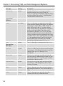
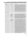
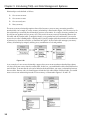
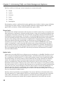
AL
1
MA
TE
RI
Introducing T - SQL and Data
Management Systems
GH
TE
D
This first chapter introduces you to some of the fundamentals of the design and architecture of
relational databases and presents a brief description of SQL as a language. If you are new to SQL
and database technologies, this chapter will provide a foundation to help ensure the rest of the
book is as useful as possible. If you are already comfortable with the concepts of relational
databases and Microsoft’s implementation, you might want to skip ahead to Chapter 2,
“SQL Server Fundamentals,” or Chapter 3, “SQL Server Tools.” Both of these chapters introduce
the features and tools in SQL Server 2005 and 2008 and discuss how they are used to write T-SQL.
RI
T - SQL Language
CO
PY
I have mentioned to my colleagues and anyone else who might have been listening that one
day I was going to write a version of Parker Brother ’s Trivial Pursuit entitled “Trivial Pursuit:
Geek Edition.” This section gives you some background on the T-SQL language and provides the
information you need to get the orange history wedge on the topic of “Database History” in Trivial
Pursuit: Geek Edition.
T-SQL is Microsoft’s implementation of a standard established by the American National
Standards Institute (ANSI) for the Structured Query Language (SQL). SQL was first developed by
researchers at IBM. They called their first pre-release version of SQL “SEQUEL,” which is a
pseudo-acronym for Structured English QUEry Language. The first release version was renamed
to SQL, dropping the English part but retaining the pronunciation to identify it with its
predecessor. As of the release of SQL Server 2008, several implementations of SQL by different
stakeholders are in the database marketplace. As you sojourn through the sometimes mystifying
lands of database technology you will undoubtedly encounter these different varieties of SQL.
What makes them all similar is the ANSI standard to which IBM, more than any other vendor,
adheres to with tenacious rigidity. However, what makes the many implementations of SQL
different are the customized programming objects and extensions to the language that make it
unique to that particular platform.
Chapter 1: Introducing T-SQL and Data Management Systems
Microsoft SQL Server 2008 implements the 2003 ANSI standard. The term “implements” is of
significance. T-SQL is not fully compliant with ANSI standards in any of its implementations; neither is
Oracle’s P/L SQL, Sybase’s SQLAnywhere, or the open-source MySQL. Each implementation has
custom extensions and variations that deviate from the established standard. ANSI has three levels of
compliance: Entry, Intermediate, and Full. T-SQL is certified at the entry level of ANSI compliance. If you
strictly adhere to the features that are ANSI-compliant, the same code you write for Microsoft SQL
Server should work on any ANSI-compliant platform; that’s the theory, anyway. If you find that you are
writing cross-platform queries, you will most certainly need to take extra care to ensure that the syntax is
perfectly suited for all the platforms it affects. The simple reality of this issue is that very few people will
need to write queries to work on multiple database platforms. The standards serve as a guideline to help
keep query languages focused on working with data, rather than other forms of programming. This may
slow the evolution of relational databases just enough to keep us sane.
Programming Language or Query Language?
T-SQL was not really developed to be a full-fledged programming language. Over the years, the ANSI
standard has been expanded to incorporate more and more procedural language elements, but it still
lacks the power and flexibility of a true programming language. Antoine, a talented programmer and
friend of mine, refers to SQL as “Visual Basic on Quaaludes.” I share this bit of information not because
I agree with it, but because I think it is funny. I also think it is indicative of many application developers’
view of this versatile language.
T-SQL was designed with the exclusive purpose of data retrieval and data manipulation.
Although T-SQL, like its ANSI sibling, can be used for many programming-like operations, its
effectiveness at these tasks varies from excellent to abysmal. That being said, I am still more than
happy to call T-SQL a programming language if only to avoid someone calling me a SQL “queryers.”
However, the undeniable fact still remains: as a programming language, T-SQL falls short. The good
news is that as a data retrieval and set manipulation language it is exceptional. When T-SQL
programmers try to use T-SQL like a programming language, they invariably run afoul of the best
practices that ensure the efficient processing and execution of the code. Because T-SQL is at its best when
manipulating sets of data, try to keep that fact foremost in your thoughts during the process of
developing T-SQL code.
With the release of SQL Server 2005, Microsoft muddied the waters a bit with the ability to write calls to
the database in a programming language like C# or VB.NET, rather than in pure SQL. SQL Server 2008
also supports this very flexible capability, but use caution! Although this is a very exciting innovation in
data access, the truth of the matter is that almost all calls to the database engine must still be
manipulated so that they appear to be T-SQL based.
Performing multiple recursive row operations or complex mathematical computations is quite possible
with T-SQL, but so is writing a .NET application with Notepad. When I was growing up my father used
to make a point of telling me that “Just because you can do something doesn’t mean you should.” The
point here is that oftentimes SQL programmers will resort to creating custom objects in their code that
are inefficient as far as memory and CPU consumption are concerned. They do this because it is the
easiest and quickest way to finish the code. I agree that there are times when a quick solution is the best,
but future performance must always be taken into account.
One of the systems I am currently working on is a perfect example of this problem. The database started
out very small, with a small development team and a small number of customers using the database. It
worked great. However, the database didn’t stay small, and as more and more customers started using
2
Chapter 1: Introducing T-SQL and Data Management Systems
the system, the number of transactions and code executions increased exponentially. It wasn’t long
before inefficient code began to consume all the available CPU resources. This is the trap of writing
expedient code instead of efficient code. Another of my father ’s favorite sayings is “Why is there never
enough time to do the job right, but plenty of time to do it twice?” This book tries to show you the best
way to write T-SQL so that you can avoid writing code that will bring your server to its knees, begging
for mercy. Don’t give in to the temptation to write sloppy code just because it is a “one time deal.” I have
seen far too many times when that one-off ad-hoc query became a central piece of an application’s
business logic.
What’s New in SQL Server 2008
When SQL Server 2005 was released, it had been five years since the previous release and the changes to
the product since the release of SQL Server 2000 were myriad and significant. Several books and
hundreds of websites were published that were devoted to the topic of “What’s New in SQL Server 2005.”
With the release of SQL Server 2008, however, there is much less buzz and not such a dramatic change
to the platform. However, the changes in the 2008 release are still very exciting and introduce many
changes that T-SQL and application developers have been clamoring for. Since these changes are
sprinkled throughout the capabilities of SQL Server, I won’t spend a great deal of time describing all the
changes here. Instead, throughout the book I will identify those changes that are applicable to the subject
being described. In this introductory chapter I want to quickly mention two of the significant changes to
SQL that will invariably have an impact on the SQL programmer: the incorporation of the .NET
Framework with SQL Server and the introduction of Microsoft Language Integrated Query (LINQ).
Kiss T-SQL Goodbye?
I have been hearing for years that T-SQL and its ANSI counterpart, SQL, were antiquated languages and
would soon be phased out. However, every database vendor, both small and large, has devoted millions
of dollars to improving their version of this versatile language. Why would they do that if it were a dead
language? The simple fact of the matter is that databases are built and optimized for the set-based
operations that the SQL language offers. Is there a better way to access and manipulate data? Probably so,
but with every major industry storing their data in relational databases, the reign of SQL is far from over.
I worked for a great guy at a Microsoft partner company who was contracted by Microsoft to develop
and deliver a number of SQL Server and Visual Studio evangelism presentations. Having a background
in radio sales and marketing, he came up with a cool tagline about SQL Server and the .NET Framework
that said “SQL Server and .NET — Kiss T-SQL Goodbye.” He was quickly dissuaded by his team when
presented with the facts. However, Todd wasn’t completely wrong. What his catchy tagline could have
said and been accurate was “SQL Server and .NET — Kiss Inefficient, CPU-Hogging T-SQL Code
Goodbye.”
Two significant improvements in data access over the last two releases of SQL Server have offered fuel
for the “SQL is dead” fire. As I mentioned briefly before, these are the incorporation of the .NET
Framework and the development of LINQ. LINQ is Microsoft’s latest application data-access technology.
It enables Visual Basic and C# applications to use set-oriented queries that are developed in C# or VB,
rather than requiring that the queries be written in T-SQL. Building in the .NET Framework to the SQL
Server engine enables developers to create SQL Server programming objects such as stored procedures,
functions, and aggregates using any .NET language and compiling them into Common Language
Runtime (CLR) assemblies that can be referenced directly by the database engine.
3
Chapter 1: Introducing T-SQL and Data Management Systems
So with the introduction of LINQ in SQL Server 2008 and CLR integration in SQL Server 2005, is T-SQL
on its death bed? No, not really. Reports of T-SQL’s demise are premature and highly exaggerated. The
ability to create database programming objects in managed code instead of SQL does not mean that
T-SQL is in danger of becoming extinct. Likewise, the ability to create set-oriented queries in C# and VB
does not sound the death knell for T-SQL. SQL Server ’s native language is still T-SQL. LINQ will help
in the rapid development of database applications, but it remains to be seen if this technology will match
the performance of native T-SQL code run from the server. This is because LINQ data access still must be
translated from the application layer to the database layer, but T-SQL does not. It’s a fantastic and
flexible access layer for smaller database applications, but for large, enterprise-class applications, LINQ,
like embedded SQL code in applications before it, falls short of pure T-SQL in terms of performance.
What was true then is true now. T-SQL will continue to be the core language for applications that need to
add, extract, and manipulate data stored on SQL Server. Until the data engine is completely re-engineered
(and that day will inevitably come), T-SQL will be at the heart of SQL Server.
Database Management Systems
A database management system (DBMS) is a set of programs designed to store and maintain data. The
role of the DBMS is to manage the data so that the consistency and integrity of the data is maintained
above all else. Quite a few types and implementations of database management systems exist:
4
❑
Hierarchical database management systems (HDBMS) — Hierarchical databases have been
around for a long time and are perhaps the oldest of all databases. They were (and in some cases
still are) used to manage hierarchical data. They have several limitations, such as being able to
manage only single trees of hierarchical data and the inability to efficiently prevent erroneous or
duplicate data. HDBMS implementations are getting increasingly rare and are constrained to
specialized, and typically non-commercial, applications.
❑
Network database management system (NDBMS) — The NDBMS has been largely abandoned.
In the past, large organizational database systems were implemented as network or hierarchical
systems. The network systems did not suffer from the data inconsistencies of the hierarchical
model, but they did suffer from a very complex and rigid structure that made changes to the
database or its hosted applications very difficult.
❑
Relational database management system (RDBMS) — An RDBMS is a software application
used to store data in multiple related tables using SQL as the tool for creating, managing, and
modifying both the data and the data structures. An RDBMS maintains data by storing it in
tables that represent single entities, such as “Customer” and “Sale” and storing information
about the relationship of these tables to each other in yet more tables managed by the system
which define the relationship between the Sale table and the Customer table. The concept of a
relational database was first described by E. F. Codd, an IBM scientist who defined the relational
model in 1970. Relational databases are optimized for recording transactions and the resultant
transactional data. Most commercial software applications use an RDBMS as their data store.
Because SQL was designed specifically for use with an RDBMS, I will spend a little extra time
covering the basic structures of an RDBMS later in this chapter.
❑
Object-oriented database management system (ODBMS) — The ODBMS emerged a few years
ago as a system where data was stored as objects in a database. ODBMS supports multiple classes
of objects and inheritance of classes along with other aspects of object orientation. Currently, no
international standard exists that specifies exactly what an ODBMS is and what it isn’t.
Chapter 1: Introducing T-SQL and Data Management Systems
Because ODBMS applications store objects instead of related entities, they make the system very
efficient when dealing with complex data objects and object-oriented programming (OOP)
languages such as the .NET languages from Microsoft as well as C and Java. When ODBMS
solutions were first released, they were quickly touted as the ultimate database system and
predicted to make all other database systems obsolete. However, they never achieved the wide
acceptance that was predicted. They do have a very valid position in the database market, but it
is a niche market held mostly within the Computer-Aided Design (CAD) and
telecommunications industries.
❑
Object-relational database management system (ORDBMS) — The ORDBMS emerged from
existing RDBMS solutions when the vendors who produced the relational systems realized that
the ability to store objects was becoming more important. They incorporated mechanisms to be
able to store classes and objects in the relational model. ORDBMS implementations have, for the
most part, usurped the market that the ODBMS vendors were targeting for a variety of reasons
that I won’t expound on here. However, Microsoft’s SQL Server, with its xml data type, the
incorporation of the .NET Framework, and the new filestream data type introduced with SQL
Server 2008, could arguably be labeled an ORDBMS. The filestream data type is discussed in
more detail later in this chapter and in Appendix E.
SQL Ser ver as a Relational Database
Management System
This section introduces you to the concepts behind relational databases and how they are implemented
from a Microsoft viewpoint. This will, by necessity, skirt the edges of database object creation, which is
covered in great detail in Chapter 13, so for the purpose of this discussion I will avoid the exact
mechanics and focus on the final results.
As I mentioned earlier, a relational database stores all its data inside tables. Ideally, each table will
represent a single entity or object. You would not want to create one table that contained data about both
dogs and cars. That isn’t to say you couldn’t do this, but it wouldn’t be very efficient or easy to maintain
if you did.
Tables
Tables are divided up into rows and columns. Each row must be able to stand on its own, without a
dependency to other rows in the table. The row must represent a single, complete instance of the entity
the table was created to represent. Each column in the row contains specific attributes that help define the
instance. This may sound a bit complex, but it is actually very simple. To help illustrate, consider a
real-world entity, such as an employee. If you want to store data about an employee, you would need to
create a table that has the properties you need to record data about your employee. For simplicity’s sake,
call your table Employee.
When you create your employee table, you also need to decide which attributes of the employee you
want to store. For the purposes of this example, suppose that you have decided to store the employee’s
last name, first name, Social Security number, department, extension, and hire date. The resulting table
would look something like that shown in Figure 1-1.
5
Chapter 1: Introducing T-SQL and Data Management Systems
Figure 1-1
The data in the table would look something like that shown in Figure 1-2.
Figure 1-2
Primary Keys
To manage the data in your table efficiently, you need to be able to uniquely identify each individual row
in the table. It is much more difficult to retrieve, update, or delete a single row if there is not a single
attribute that identifies each row individually. In many cases, this identifier is not a descriptive attribute
of the entity. For example, the logical choice to uniquely identify your employee is the Social Security
number attribute. However, there are a couple of reasons why you would not want to use the Social
Security number as the primary mechanism for identifying each instance of an employee, both boiling
down to two different areas: security and efficiency.
When it comes to security, what you want to avoid is the necessity of securing the employee’s Social
Security number in multiple tables. Because you will most likely be using the key column in multiple
tables to form your relationships (more on that in a moment), it makes sense to substitute a nondescriptive key. In this way you avoid the issue of duplicating private or sensitive data in multiple
locations to provide the mechanism to form relationships between tables.
As far as efficiency is concerned, you can often substitute a non-data key that has a more efficient or
smaller data type associated with it. For example, in your design you might have created the Social
Security number with either a character data type or an integer. If you have fewer than 32,767
employees, you can use a double-byte integer instead of a 4-byte integer or 10-byte character type;
besides, integers process faster than characters.
So, instead of using the Social Security number, you will assign a non-descriptive key to each row. The
key value used to uniquely identify individual rows in a table is called a primary key. (You will still
want to ensure that every Social Security number in your table is unique and not null, but you will use a
different method to guarantee this behavior without making it a primary key.)
A non-descriptive key doesn’t represent anything else with the exception of being a value that uniquely
identifies each row or individual instance of the entity in a table. This will simplify the joining of this
table to other tables and provide the basis for a “relation.” In this example you will simply alter the table
by adding an EmployeeKey column that will uniquely identify every row in the table, as shown in
Figure 1-3.
6
Chapter 1: Introducing T-SQL and Data Management Systems
Figure 1-3
With the EmployeeKey column, you have an efficient, easy-to-manage primary key.
Each table can have only one primary key, which means that this key column is the primary method for
uniquely identifying individual rows. It doesn’t have to be the only mechanism for uniquely identifying
individual rows; it is just the “primary” mechanism for doing so. Primary keys can never be null, and
they must be unique. Primary keys can also be combinations of columns (though I’ll explain later why
I am a firm believer that primary keys should typically be single-column keys). If you have a table where
two columns in combination are unique, while either single column is not, you can combine the two
columns as a single primary key, as illustrated in Figure 1-4.
Figure 1-4
In this example, the LibraryBook table is used to maintain a record of every book in the library. Because
multiple copies of each book can exist, the ISBN column is not useful for uniquely identifying each book.
To enable the identification of each individual book, the table designer decided to combine the ISBN
column with the copy number of each book. Personally, I avoid the practice of using multiple column
keys. I prefer to create a separate column that can uniquely identify the row. This makes it much easier to
write join queries (covered in detail in Chapter 8). The resulting code is cleaner and the queries are
generally more efficient. For the library book example, a more efficient mechanism might be to assign
each book its own number. The resulting table would look like that shown in Figure 1-5.
Figure 1-5
7
Chapter 1: Introducing T-SQL and Data Management Systems
Table Columns
As previously described, a table is a set of rows and columns used to represent an entity. Each
row represents an instance of the entity. Each column in the row will contain at most one value that
represents an attribute, or property, of the entity. For example, consider the employee table; each
row represents a single instance of the employee entity. Each employee can have one and only one first
name, last name, SSN, extension, or hire date, according to your design specifications. In addition to
deciding which attributes you want to maintain, you must also decide how to store those attributes.
When you define columns for your tables, you must, at a minimum, define three things:
❑
The name of the column
❑
The data type of the column
❑
Whether the column can support null
Column Names
Keep the names simple and intuitive (such as LastName or EmployeeID) instead of more cumbersome
names (such as EmployeeLastName and EmployeeIdentificationNumber). For more information,
see Chapter 8.
Data Types
The general rule on data types is to use the smallest one you can. This conserves memory usage and disk
space. Also keep in mind that SQL Server processes numbers much more efficiently than characters, so
use numbers whenever practical. I have heard the argument that numbers should be used only if you
plan on performing mathematical operations on the columns that contain them, but that just doesn’t
wash. Numbers are preferred over string data for sorting and comparison as well as mathematical
computations. The exception to this rule is if the string of numbers you want to use starts with a zero.
Take the Social Security number, for example. Other than the unfortunate fact that some Social Security
numbers begin with a zero, the Social Security number would be a perfect candidate for using an integer
instead of a character string. However, if you tried to store the integer 012345678, you would end up
with 12345678. These two values may be numeric equivalents, but the government doesn’t see it that
way. They are strings of numerical characters and therefore must be stored as characters rather than as
numbers.
When designing tables and choosing a data type for each column, try to be conservative and use the
smallest, most efficient type possible. But at the same time, carefully consider the exception, however
rare, and make sure that the chosen type will always meet these requirements.
The data types available for columns in SQL Server 2005 and 2008 are specified in the following table.
Those that are unique to SQL Server 2008 are prefixed with an asterisk (*).
8
Chapter 1: Introducing T-SQL and Data Management Systems
Data Type
Storage
Description
Note: Signed integers can be both positive and negative,
whereas unsigned integers have no inherent signed value
Integers
bigint
8 bytes
An 8-byte signed integer. Valid values are
−9223372036854775808 through +9223372036854775807.
int
4 bytes
A 4-byte signed integer. Valid values are −2,147,483,648
through +2,147,483,647.
smallint
2 bytes
A double-byte signed integer. Valid values are −32,768
through +32,767.
tinyint
1 byte
A single-byte unsigned integer. Valid values are from
0 through 255.
bit
1 bit
Integer data with either a 1 or 0 value.
decimal
5–17 bytes
A predefined, fixed, signed decimal number ranging from
−100000000000000000000000000000000000001 (−1038+1) to
99999999999999999999999999999999999999 (+1038−1).
A decimal is declared with a precision and scale value that
determines how many decimal places to the left and right
are supported. This is expressed as decimal[(precision,
[scale])]. The precision setting determines how
many total digits to the left and right of the decimal point
are supported. The scale setting determines how many
digits to the right of the decimal point are supported. For
example, to support the number 3.141592653589793,
the decimal data type would have to be specified as
decimal(16,15). If the data type were specified
as decimal(3,2), only 3.14 would be stored. The scale
defaults to zero and must be between 0 and the precision.
The precision defaults to 18 and can be a maximum of 38.
numeric
5–17 bytes
The numeric data type is identical to the decimal data
type, so use decimal instead, for consistency. The
numeric data type is much less descriptive because
most people think of integers as being numeric.
money
8 bytes
The money data type can be used to store values from
−922,337,203,685,477.5808 to +922,337,203,685,477.5807 of
a monetary unit, such as a dollar, euro, pound, and so on.
The advantage of the money data type over a decimal
data type is that developers can take advantage of
automatic currency formatting for specific locales. Notice
that the money data type supports figures to the fourth
decimal place. Accountants like that. A few million of
those ten thousandths of a penny add up after a while!
Exact Numerics
(continued)
9
Chapter 1: Introducing T-SQL and Data Management Systems
Data Type
Storage
Description
smallmoney
4 bytes
Bill Gates needs the money data type to track his
portfolio, but most of us can get by with the
smallmoney data type. It consumes 4 bytes of storage
and can be used to store values of −214,748.3648 to
+214,748.3647 of a monetary unit.
float
4 or 8 bytes
The float data type is an approximate value (SQL
Server performs rounding) that supports real numbers
in the range of −1.79E + 308 to −2.23E − 308, 0 and
2.23E − 308 to 1.79E + 308. float can be used as a
4-byte or 8-byte data type, depending on an optional
mantissa value (the number of bits used to store
the mantissa of the float). float(24) or any value
between 1 and 24 will cause the float to be defined as
a 4-byte value that can store real numbers in the range
of −3.40E + 38 to −1.18E − 38, 0 and 1.18E − 38 to 3.40E
+ 38. Any number between 25 and 53 will cause the
float to be defined as an 8-bit float (aka, a double
precision) in the default manner of float(53).
real
4 bytes
The real data type is a synonym for a 4-byte float.
datetime
8 bytes
The datetime data type is used to store date and time
from January 1, 1753 through December 31, 9999. The
accuracy of the datetime data type is 3.33
milliseconds.
*datetime2
8 bytes
The datetime2 data type is used to store date and
time from January 1, 0001 through December 31, 9999.
The accuracy of the datetime2 data type is variable
but defaults to 100 nanoseconds.
smalldatetime
4 bytes
The smalldatetime data type stores date and time
from January 1, 1900 through June 6, 2079, with an
accuracy of 1 minute.
*date
3 bytes
The date data type stores dates only from January 1,
0001 through December 31, 9999, with an accuracy of
1 day.
*time
5 bytes
The time data type stores time-only data, with a
variable precision of up to 100 nanoseconds
Approximate
Numerics
Date and Time
Data Types
10
Chapter 1: Introducing T-SQL and Data Management Systems
Data Type
Storage
Description
*datetimeoffset
10 bytes
The datetimeoffset data type is used to store date
and time from January 1, 0001 through December 31,
9999. The accuracy of the datetimeoffset data type
varies based on the type of server hardware SQL Server
is installed on, but defaults to 100 nanoseconds if
supported. When defined, the datetimeoffset data
type expects a date and time string to be specified
along with a time zone offset. Possible time zone offsets
are between −14.00 and +14.00 hours. For example, to
define a variable that is time-zone aware for Pacific
Standard Time, the following code would be used:
DECLARE @PacificTime AS datetimeoffset(8)
Character Data Types
char
1 byte per
character.
Maximum
8000
characters.
The char data type is a fixed-length data type used to
store character data. The number of possible characters is
between 1 and 8000. The possible combinations of
characters in a char data type are 256. The characters that
are represented depend on what language, or collation, is
defined. English, for example, is actually defined with a
Latin collation. The Latin collation provides support for
all English and western European characters.
varchar
1 byte per
character. Up
to 2GB
characters.
The varchar data type is identical to the char data
type, but with a variable length. If a column is defined
as char(8), it will consume 8 bytes of storage even if
only three characters are placed in it. A varchar
column consumes only the space it needs. Typically,
char data types are more efficient when it comes to
processing and varchar data types are more efficient
for storage. The rule of thumb is to use char if the data
will always be close to the defined length, but use
varchar if it will vary widely. For example, a city name
would be stored with varchar(167) if you wanted to
allow for the longest city name in the world, which is
Krung thep mahanakhon bovorn ratanakosin
mahintharayutthaya mahadilok pop noparatratchathani
burirom udomratchanivetmahasathan amornpiman
avatarnsathit sakkathattiyavisnukarmprasit (the poetic
name of Bangkok, Thailand). Use char for data that is
always the same. For example, you could use char(12)
to store a domestic phone number in the United States:
(123)456-7890. The 8000-byte limitation can be exceeded
by specifying the (MAX) option (varchar(MAX)),
which allows for the storage of 2,147,483,647 characters
at the cost of up to 2GB storage space.
(continued)
11
Chapter 1: Introducing T-SQL and Data Management Systems
Data Type
Storage
Description
text
1 byte per
character.
Maximum
2,147,483,648
characters
(2GB).
The text data type is similar to the varchar data type
in that it is a variable-length character data type. The
significant difference is the maximum length of about
2 billion characters (including spaces) and where the
data is physically stored. With a varchar data type on
a table column, the data is stored physically in the row
with the rest of the data. With a text data type, the
data is stored separately from the actual row and a
pointer is stored in the row so that SQL Server can find
the text. The text data type is functionally equivalent
to the varchar(MAX) data type.
nchar
2 bytes per
character.
Maximum
4000
characters
(8000 bytes).
The nchar data type is a fixed-length type identical to
the char data type, with the exception of the number of
characters supported. char data is represented by a
single byte and thus only 256 different characters can be
supported. nchar is a double-byte data type and can
support 65,536 different characters. The cost of the extra
character support is the double-byte length, so the
maximum nchar length is 4000 characters or 8000 bytes.
nvarchar
2 bytes per
character. Up
to 2GB.
The nvarchar data type is a variable-length type
identical to the varchar data type, with the exception
of the amount of characters supported. varchar data
is represented by a single byte and only 256 different
characters can be supported. nvarchar is a doublebyte data type and can support 65,536 different
characters. The cost of the extra character support is
the double-byte length, so the maximum nvarchar
length is 4000 characters or 8000 bytes. This limit can
be exceeded by using the (MAX) option, which allows
for the storage of 1,073,741,823 characters in 2GB.
ntext
2 bytes per
character.
Maximum
1,073,741,823
characters.
The ntext data type is identical to the text data type,
with the exception of the number of characters
supported. text data is represented by a single byte and
only 256 different characters can be supported. ntext is a
double-byte data type and can support 65,536 different
characters. The cost of the extra character support is the
double-byte length, so the maximum ntext length is
1,073,741,823 characters or 2GB. The ntext data type is
functionally equivalent to the nvarchar(MAX) data type.
1–8000 bytes
Fixed-length binary data. Length is fixed when created
between 1 and 8000 bytes. For example, binary(5000)
specifies the reserving of 5000 bytes of storage to
accommodate up to 5000 bytes of binary data.
Binary Data Types
binary
12
Chapter 1: Introducing T-SQL and Data Management Systems
Data Type
Storage
Description
varbinary
Up to
2,147,483,647
bytes
Variable-length binary data type identical to the
binary data type, with the exception of consuming
only the amount of storage that is necessary to hold
the data. Using the (MAX) option allows for the
storage of up to 2GB of binary data. However, only 1
through 8000 or MAX can be specified as storage
options.
image
Up to
2,147,483,647
bytes
The image data type is similar to the varbinary
data type in that it is a variable-length binary data
type. The significant difference is the maximum length
of about 2GB and where the data is physically stored.
With a varbinary data type on a table column, the
data is stored physically in the row with the rest of the
data. With an image data type, however, the data is
stored separately from the actual row and a pointer
is stored in the row so that SQL Server can find the
data. Typically, image data types are used to store
actual images, binary documents, or binary objects.
The image data type is functionally identical to
varbinary(MAX).
timestamp
8 bytes
The timestamp data type has nothing to do with
time. It is more accurately described as a data
type that maintains row version data. In light of this
fact, a system alias of rowversion is available for
this data type and is generally preferred to avoid
confusion. What timestamp actually provides is
a database unique identifier to identify a version of a
row. Every time a row that contains a timestamp data
type is modified, the value of the timestamp changes.
uniqueidentifier
32 bytes
A data type used to store a globally unique identifier
(GUID).
*hierarchyid
Up to 892
bytes
The hierarchyid data type is a variable length data
type that is used to represent position in a hierarchy.
sql_variant
Up to 8016
bytes
sql_variant is used when the exact data type is
Up to 2GB
The xml data type is used to store well-formed
XML. The XML stored can be specified to be wellformed fragments or complete documents and can be
enforced with an XML schema bound to the variable,
parameter, or column containing the XML data.
Other Data Types
xml
unknown. It can be used to hold any data type with
the exception of text, ntext, image, and timestamp.
13
Chapter 1: Introducing T-SQL and Data Management Systems
SQL Server supports additional data types, listed in the following table, that can be used in queries and
programming objects, but they are not used to define columns.
Data Type
Description
cursor
The cursor data type is used to point to an instance of a cursor.
table
The table data type is used to store an in-memory rowset for processing. It was
developed primarily for use with the table-valued functions that were introduced
in SQL Server 2000.
Nullability
All rows from the same table have the same set of columns. However, not all columns will necessarily
have values in them. For example, a new employee is hired, but he has not been assigned an extension
yet. In this case, the extension column may not have any data in it. Instead, it may contain null, which
means the value for that column was not initialized. Note that a null value for a string column is
different from an empty string. An empty string is defined; a null is not. You should always consider a
null as an unknown value. When you design your tables, you need to decide whether to allow a null
condition to exist in your columns. Nulls can be allowed or disallowed on a column-by-column basis, so
your employee table design could look like that shown in Figure 1-6.
Figure 1-6
Relationships
Relational databases are all about relations. To manage these relations, you use common keys. For
example, your employees sell products to customers. This process involves multiple entities:
❑
The employee
❑
The product
❑
The customer
❑
The sale
To identify which employee sold which product to which customer, you need some way to link together
all the entities. Typically, these links are managed through the use of keys — primary keys in the parent
table and foreign keys in the child table.
14
Chapter 1: Introducing T-SQL and Data Management Systems
As a practical example, you can revisit the employee example. When your employee sells a product, his or
her identifying information is added to the Sale table to record who the responsible employee was, as
illustrated in Figure 1-7. In this case, the Employee table is the parent table and the Sale table is the child table.
Figure 1-7
Because the same employee could sell products to many customers, the relationship between the
Employee table and the Sale table is called a one-to-many relationship. The fact that the employee is the
unique participant in the relationship makes it the parent table. Relationships are very often parent-child
relationships, which means that the record in the parent table must exist before the child record can be
added. In the example, because every employee is not required to make a sale, the relationship is more
accurately described as a one-to-zero-or-more relationship. In Figure 1-7 this relationship is represented
by a key and infinity symbol, which doesn’t adequately model the true relationship because you don’t
know if the EmployeeKey field is nullable. In Figure 1-8, the more traditional and informative “crows
feet” symbol is used. The relationship symbol in this figure represents an exactly one (the double vertical
lines) to zero (the ring) or more (the crows feet) relationship. Figure 1-9 shows the two tables with an
exactly one to one or more relationship symbol. The PK abbreviation stands for primary key, while the
FK stands for foreign key. Because a table can have multiple foreign keys, they are numbered
sequentially starting at 1.
Figure 1-8
Figure 1-9
15
Chapter 1: Introducing T-SQL and Data Management Systems
Relationships can be defined as follows:
❑
One-to-zero or more
❑
One-to-one or more
❑
One-to-exactly-one
❑
Many-to-many
The many-to-many relationship requires three tables because a many-to-many constraint would be
unenforceable. An example of a many-to-many relationship is illustrated in Figure 1-10. The necessity for
this relationship is created by the relationships between your entities: In a single sale many products can
be sold, but one product can be in many sales. This creates the many-to-many relationship between the
Sale table and the Product table. To uniquely identify every product and sale combination, you need to
create what is called a linking table. A linking table is simply another table that contains the combination
of primary keys from the two tables, as illustrated in Figure 1-10. The Order table manages your manyto-many relationship by uniquely tracking every combination of sale and product.
Figure 1-10
As an example of a one-to-one relationship, suppose that you want to record more detailed data about a
sale, but you do not want to alter the current table. In this case, you could build a table called SaleDetail to
store the data. To ensure that the sale can be linked to the detailed data, you create a relationship between
the two tables. Because each sale should appear in both the Sale table and the SaleDetail table, you would
create a one-to-one relationship instead of a one-to-many, as illustrated in Figures 1-11 and 1-12.
Figure 1-11
Figure 1-12
16
Chapter 1: Introducing T-SQL and Data Management Systems
RDBMS and Data Integrity
An RDBMS is designed to maintain data integrity in a transactional environment. This is accomplished
through several mechanisms implemented through database objects. The most prominent of these
objects are as follows:
❑
Locks
❑
Constraints
❑
Keys
❑
Indexes
Before I describe these objects in more detail, it’s important to understand two other important pieces of
the SQL architecture: connections and transactions.
Connections
A connection is created anytime a process attaches to SQL Server. The connection is established with
defined security and connection properties. These security and connection properties determine which
data you have access to and to a certain degree, how SQL Server will behave during the duration of the
query in the context of the query. For example, a connection can specify which database to connect to on
the server and how to manage memory-resident objects.
Transactions
Transactions are explored in detail in Chapter 10, so for the purposes of this introduction I will keep the
explanation brief. In a nutshell, a SQL Server transaction is a collection of dependent data modifications
that is controlled so that it completes entirely or not at all. For example, you go to the bank and transfer
$100.00 from your savings account to your checking account. This transaction involves two
modifications — one to the checking account and the other to the savings account. Each update is
dependent on the other. It is very important to you and the bank that the funds are transferred correctly,
so the modifications are placed together in a transaction. If the update to the checking account fails but
the update to the savings account succeeds, you most definitely want the entire transaction to fail. The
bank feels the same way if the opposite occurs.
With a basic idea about these two objects, let’s proceed to the four mechanisms that ensure integrity and
consistency in your data.
Locks
SQL Server uses locks to ensure that multiple users can access data at the same time with the
assurance that the data will not be altered while they are reading it. At the same time, the locks are used
to ensure that modifications to data can be accomplished without affecting other modifications or reads
in progress. SQL Server manages locks on a connection basis, which simply means that locks cannot be
held mutually by multiple connections. SQL Server also manages locks on a transaction basis. In the
same way that multiple connections cannot share the same lock, neither can transactions. For example, if
an application opens a connection to SQL Server and is granted a shared lock on a table, that same
application cannot open an additional connection and modify that data. The same is true for
transactions. If an application begins a transaction that modifies specific data, that data cannot be
modified in any other transaction until the first has completed its work. This is true even if the multiple
transactions share the same connection.
17
Chapter 1: Introducing T-SQL and Data Management Systems
SQL Server utilizes six lock types, or more accurately, six resource lock modes:
❑
Shared
❑
Update
❑
Exclusive
❑
Intent
❑
Schema
❑
Bulk Update
Shared, update, exclusive, and intent locks can be applied to rows of tables or indexes, pages (8-kilobyte
storage page of an index or table), extents (64-kilobyte collection of eight contiguous index or table
pages), tables, or databases. Schema and bulk update locks apply to tables.
Shared Locks
Shared locks allow multiple connections and transactions to read the resources they are assigned to. No
other connection or transaction is allowed to modify the data as long as the shared lock is granted. Once
an application successfully reads the data, the shared locks are typically released, but this behavior can
be modified for special circumstances. For instance, a shared lock might be held for an entire transaction
to ensure maximum protection of data consistency by guaranteeing that the data that a transaction is
based on will not change until the transaction is completed. This extended locking is useful for situations
where transactional consistency must be 100% assured, but the cost of holding the locks is that
concurrent access to data is reduced. For example, you want to withdraw $100.00 from your savings
account. A shared lock is issued on the table that contains your savings account balance. That data is
used to confirm that there are enough funds to support the withdrawal. It would be advantageous to
prevent any other connection from altering the balance until after the withdrawal is complete. Shared
locks are compatible with other shared locks so that many transactions and connections can read the
same data without conflict.
Update Locks
Update locks are used by SQL Server to help prevent an event known as a deadlock. Deadlocks are bad.
They are mostly caused by poor programming techniques. A deadlock occurs when two processes get
into a standoff over shared resources. Let’s return to the banking example: In this hypothetical banking
transaction both my wife and I go online to transfer funds from our savings account to our checking
account. We somehow manage to execute the transfer operation simultaneously and two separate
processes are launched to execute the transfer. When my process accesses the two accounts, it is issued
shared locks on the resources. When my wife’s process accesses the accounts, it is also granted a shared
lock to the resources. So far, so good, but when our processes try to modify the resources, pandemonium
ensues. First my wife’s process attempts to escalate its lock to exclusive to make the modifications. At
about the same time my process attempts the same escalation. However, our mutual shared locks
prevent either of our processes from escalating to an exclusive lock. Because neither process is willing to
release its shared lock, a deadlock occurs.
SQL Server doesn’t particularly care for deadlocks. If one occurs, SQL Server will automatically select
one of the processes as a victim and kill it. SQL Server selects the process with the least cost associated
with it, kills it, rolls back the associated transaction, and notifies the responsible application of the
termination by returning error number 1205. If properly captured, this error informs the user that
18
Chapter 1: Introducing T-SQL and Data Management Systems
“Transaction ## was deadlocked on x resources with another process and has been chosen as the
deadlock victim. Rerun the transaction.” To avoid the deadlock from ever occurring, SQL Server will
typically use update locks in place of shared locks. Only one process can obtain an update lock,
preventing the opposing process from escalating its lock. The bottom line is that if a read is executed for
the sole purpose of an update, SQL Server may issue an update lock instead of a shared lock to avoid a
potential deadlock. This can all be avoided through careful planning and implementation of SQL logic
that prevents the deadlock from ever occurring.
Exclusive Locks
SQL Server typically issues exclusive locks when a modification is executed. To change the value of a
field in a row, SQL Server grants exclusive access of that row to the calling process. This exclusive access
prevents a process from any concurrent transaction or connection from reading, updating, or deleting
the data being modified. Exclusive locks are not compatible with any other lock types.
Intent Locks
SQL Server issues intent locks to prevent a process from any concurrent transaction or connection from
placing a more exclusive lock on a resource that contains a locked resource from a separate process. For
example, if you execute a transaction that updates a single row in a table, SQL Server grants the
transaction an exclusive lock on the row, but also grants an intent lock on the table containing the row.
This prevents another process from placing an exclusive lock on the table.
Here is an analogy I often use to explain the intent lock behavior in SQL programming classes: You check
in to Room 404 at the SQL Hotel. You now have exclusive use of the fourth room on the fourth floor
(404). No other hotel patron will be allowed access to this room. In addition, no other patron will be
allowed to buy out every room in the hotel because you have already been given exclusive control to one
of the rooms. You have what amounts to an intent exclusive lock on the hotel and an exclusive lock on
Room 404. Intent locks are compatible with any less-exclusive lock, as illustrated in the following table
on lock compatibility.
Existing Granted Lock
Requested Lock Type
IS
S
U
IX
X
Intent shared (IS)
Yes
Yes
Yes
Yes
No
Shared (S)
Yes
Yes
Yes
No
No
Update(U)
Yes
Yes
No
No
No
Intent exclusive (IX)
Yes
No
No
Yes
No
Exclusive (X)
No
No
No
No
No
Schema Locks
There are two types of schema locks SQL Server will issue on a table: schema modification locks (Sch-M)
and schema stability locks (Sch-S). Schema modification locks prevent concurrent access to a table while
the table is undergoing modification — for example, a name change or a column addition. A schema
stability lock prevents the table from being modified while it is being accessed for data retrieval.
19
Chapter 1: Introducing T-SQL and Data Management Systems
Bulk Update Locks
A bulk update lock on a table allows multiple bulk load threads to load data into a table while
preventing other types of data access. Bulk update locks are issued when table locking is enabled at the
table or the chosen as an option with the bulk operation.
Key Range Locks
Key-range locks protect a range of rows implicitly included in a record set being read by a Transact-SQL
statement while using the serializable transaction isolation level. The serializable isolation level requires
that any query executed during a transaction must obtain the same set of rows every time it is executed
during the transaction. A key range lock protects this requirement by preventing other transactions from
inserting new rows whose keys would fall in the range of keys read by the serializable transaction.
SQL Ser ver and Other Products
Microsoft has plenty of competition in the client/server database world and SQL Server is a relatively
young product by comparison. However, it has enjoyed wide acceptance in the industry due to its ease
of use and attractive pricing. If our friends at Microsoft know how to do anything exceptionally well, it’s
taking a product to market so it becomes very mainstream and widely accepted.
Microsoft SQL Server
Here is a short history lesson on Microsoft’s SQL Server. Originally, SQL Server was a Sybase product
created for IBM’s OS/2 platform. Microsoft engineers worked with Sybase and IBM but eventually
withdrew from the project. Then, Microsoft licensed the Sybase SQL Server code and ported the product
to work with Windows NT. It took a couple of years before SQL Server really became a viable product.
The SQL Server team went to work to create a brand new database engine using the Sybase code as a
model. They eventually rewrote the product from scratch.
When SQL Server 7.0 was released in late 1998, it was a major departure from the previous version, SQL
Server 6.5. SQL Server 7.0 contained very little Sybase code with the exception of the core database
engine technology, which was still under license from Sybase. SQL Server 2000 was released in 2000 with
many useful new features, but was essentially just an incremental upgrade of the 7.0 product. SQL
Server 2005, however, is a major upgrade and some say it’s the very first completely Microsoft product.
Any vestiges of Sybase are long gone. The storage and retrieval engine has been completely rewritten,
the .NET Framework has been incorporated, and the product has significantly risen in both power and
scalability. SQL Server 2008 is to SQL Server 2005 what SQL Server 2000 was to SQL Server 7.0. There are
some very interesting and powerful improvements to the server, which we will address in the coming
chapters, but the changes are not as dramatic as the changes that SQL Server 2005 brought.
Oracle
Oracle is probably the most recognizable enterprise-class database product in the industry. After IBM’s
E. F. Codd published his original papers on the fundamental principles of relational data storage and
design in 1970, Larry Ellison, founder of Oracle, went to work to build a product to apply those
principles. Founded in 1977, Oracle has had a dominant place in the database market for quite some time
with a comprehensive suite of database tools and related solutions. Versions of Oracle run on UNIX,
Linux, and Windows server operating systems.
20
Chapter 1: Introducing T-SQL and Data Management Systems
The query language of Oracle is known as Procedure Language/Structured Query Language (PL/SQL).
Indeed, many aspects of PL/SQL resemble a C-like procedural programming language. This is evidenced by
syntax such as command-line termination using semicolons. Unlike T-SQL, statements are not actually
executed until an explicit run command is issued (preceded with a single line containing a period.) PL/SQL is
particular about using data types and includes expressions for assigning values to compatible column types.
IBM DB2
This is really where it all began. Relational databases and the SQL language were first conceptualized
and then implemented in IBM’s research department. Although IBM’s database products have been
around for a very long time, Oracle (then Relational Software) actually beat them to market. DB2
database professionals perceive the form of SQL used in this product to be purely ANSI SQL and other
dialects such as Microsoft’s T-SQL and Oracle’s PL-SQL to be more proprietary. Although DB2 has a long
history of running on System 390 mainframes and the AS/400, it is not just a legacy product. IBM has
effectively continued to breathe life into DB2 and it remains a viable database for modern business
solutions. DB2 runs on a variety of operating systems today, including Windows, UNIX, and Linux.
Informix
This product had been a relatively strong force in the client/server database community, but its
popularity waned in the late 1990s. Originally designed for the UNIX platform, Informix is a serious
enterprise database. Popularity slipped over the past few years, as many applications built on Informix
had to be upgraded to contend with year 2000 compatibility issues. Some organizations moving to other
platforms (such as Linux and Windows) have also switched products. The 2001 acquisition of Informix
nudged IBM to the top spot over Oracle as they brought existing Informix customers with them. Today,
Informix runs on Linux and integrates with other IBM products.
Sybase SQLAnywhere
Sybase has deep roots in the client/server database industry and has a strong product offering. At the
enterprise level, Sybase products are deployed on UNIX and Linux platforms and have strong support in
Java programming circles. At the mid-scale level, SQLAnywhere runs on several platforms, including
UNIX, Linux, Mac OS, NetWare, and Windows. Sybase has carved a niche for itself in the industry for
mobile device applications and related databases.
Microsoft Access (Jet)
To be perfectly precise, Access is not really a database platform. Access is a Microsoft Office application
that is built to use the Microsoft Jet database platform. Access and Jet were partially created from the
ground up but also leverage some of the technology gleaned from Microsoft’s acquisition of FoxPro. As a
part of Microsoft’s Office Suite, Access is a very convenient tool for creating simple business applications.
Although Access SQL is ANSI 92 SQL–compliant, it is quite a bit different from T-SQL. For this reason,
I have made it a point to identify some of the differences between Access and T-SQL throughout the book.
Access has become the non-programmer ’s application development tool. Many people get started in
database design using Access and then move on to SQL Server as their needs become more sophisticated.
Access is a powerful tool for the right kinds of applications, and some commercial products have actually
been developed using Access. Unfortunately, because Access is designed (and documented) to be an end
user ’s tool rather than a software developer ’s tool, many Access databases are often poorly designed and
power users learn through painful trial and error about how not to create database applications.
21
Chapter 1: Introducing T-SQL and Data Management Systems
The Jet Database Engine was designed in 1992. Jet is a simple and efficient storage system for small to
moderate volumes of data and for relatively few concurrent users, but it falls short of the stability and
fault-tolerance of SQL Server. For this reason, a desktop version of the SQL Server engine (now called
SQL Server Express, but formally known as Microsoft SQL Desktop Engine [MSDE]) has shipped with
Access since Office 2000. SQL Server Express is an alternative to using Jet and really should be used in
place of Jet for any serious database. Starting smaller-scale projects with SQL Server Express provides an
easier path for migrating them to full-blown SQL Server editions later on.
MySQL
MySQL is a developer ’s tool embraced by the open source community. Like Linux and Java, it can be
obtained free of charge and includes source code. Compilers and components of the database engine can
be modified and compiled to run on most any computer platform. Although MySQL supports ANSI
SQL, it promotes the use of an application programming interface (API) that wraps SQL statements. As a
database product, MySQL is a widely accepted and capable product. However, it appeals more to the
open source developer than to the business user.
Many other database products on the market may share some characteristics of the products discussed
here. The preceding list represents the most popular database products that use ANSI SQL.
Summar y
Microsoft SQL Server 2005 has earned a very good reputation in the marketplace and remains a very
capable and powerful database management server. SQL Server 2005 took T-SQL and database
management a huge step forward. Now SQL Server 2008 promises to continue the maturation of the
product with new and very powerful T-SQL commands and functions.
The upcoming chapters explore most of the longstanding features and capabilities of T-SQL and
preview the awesome new capabilities that SQL Server 2005 and SQL Server 2008 have brought to the
field of T-SQL programming. So sit back and hold on; it’s going to be an exciting ride.
If the whole idea of writing T-SQL code and working with databases doesn’t thrill you like it does me,
I apologize for my overt enthusiasm. My wife has reminded me on many occasions that no matter
how I may look, I really am a geek. I freely confess it. I also eagerly confess that I love working with
databases. Working with databases puts you in the middle of everything in information technology.
There is absolutely no better place to be. Can you name an enterprise application that doesn’t somehow
interface with a database? You see? Databases are the sun of the IT solar system!
In the coming months and years you will most likely find more and more applications storing their data
in a SQL Server database, especially if that application is carrying a Microsoft logo. Microsoft Exchange
Server doesn’t presently store its data in SQL, but it will. Active Directory will also reportedly move its
data store to SQL Server. Microsoft has been exploring for years the possibility and feasibility of moving
the Windows file system itself to a SQL-type store. For the T-SQL programmer and Microsoft SQL Server
professional, the future is indeed bright.
22