Download Meade Image Processing Technical data

Meade Autostar
Image Processing
For Windows
Version 3.12
9 January 2004
This document and the Meade Autostar IP software described herein, are copyrighted and are protected from reproduction, proliferation, and disclosure
under the Copyright laws of the United States of America.
Information in this document is subject to change without notice and does not represent a commitment on the part of Meade Instruments Corporation.
The software and/or databases described in this document are furnished under a license agreement or nondisclosure agreement. The software and/or
databases may be used or copied only in accordance with the terms of the agreement. It is against the law to copy the software on any medium except
as specifically allowed in the license or nondisclosure agreement. The purchaser may make one copy of the software for backup purposes. No part of
this manual and/or databases may be reproduced or transmitted in any form or by any means; electronic or mechanical, including photocopying,
recording, or information storage and retrieval systems, for any purpose other that the purchaser's personal use, without the express written permission
of Meade Instruments Corporation.
Copyright  1995, 2003 and 2004 by Meade Instruments All rights reserved. Printed in the United States of America.
Microsoft is a registered trademark and Windows is a trademark of Microsoft Corporation.
IBM is a registered trademark of International Business Machines.
Hewlett-Packard and LaserJet are registered trademarks of the Hewlett-Packard Company.
ACKNOWLEDGMENTS
Images have been provided by the Jet Propulsion Laboratory, Meade Instruments Corporation, Santa Barbara Instrument Group, Astrolink, Inc., SSC
Observatories and other private sources.
LIMITED WARRANTY
LIMITED WARRANTY. Meade Instruments warrants that (a) the SOFTWARE will perform substantially in accordance with the accompanying written
materials for a period of ninety (90) days from the date of receipt, and (b) any hardware accompanying the SOFTWARE will be free from defects in
materials and workmanship under normal use and service for a period of one (1) year from the date of receipt. Any implied warranties on the
SOFTWARE and hardware are limited to ninety (90) days and one (1) year respectively. Some states/countries do not allow limitations on duration of
an implied warranty, so the above limitation may not apply to you.
CUSTOMER REMEDIES. Meade Instruments and its suppliers' entire liability and your exclusive remedy shall be, at Meade 's option, either (a) repair
or (b) replacement of the SOFTWARE or hardware that does not meet Meade 's Limited Warranty and which is returned to Meade Instruments with a
copy of your receipt. This Limited Warranty is void if failure of the SOFTWARE or hardware has resulted from accident, abuse, or misapplication. Any
replacement SOFTWARE or hardware will be warranted for the remainder of the original warranty period or thirty (30) days, whichever is longer.
Outside of the United States, these remedies are not available without proof of purchase from an authorized non-U.S. source.
NO OTHER WARRANTIES. Meade Instruments and its suppliers disclaim all other warranties, either expressed or implied, including, but not
limited to, implied warranties of merchantability and fitness for a particular purpose, with regard to the SOFTWARE, the accompanying
written materials, and any accompanying hardware. This limited warranty gives you specific legal rights. You may have other rights which
vary from state/country to state/country.
NO LIABILITY FOR CONSEQUENTIAL DAMAGES. In no event shall Meade Instruments, or its suppliers, be liable for any damages
whatsoever (including without limitation, damages for loss of business profits, business interruption, loss of business information, or any
other pecuniary loss) arising out of the use of, or inability to use, the Meade product, even if Meade Instruments has been advised of the
possibility of such damages. Because some states/countries do not allow the exclusion or limitation of liability for consequential or
incidental damages, the above limitation may not apply to you.
U.S. GOVERNMENT RESTRICTED RIGHTS
The SOFTWARE and documentation are provided with RESTRICTED RIGHTS. Use, duplication, or disclosure by the Government is subject to
restriction as set forth in subparagraph (c)(1)(ii) of The Rights in Technical Data and Computer Software clause at DFARS 252.227-7013 or
subparagraphs (c)(1) and (2) of the Commercial Computer Software--Restricted Rights at 48 CFR 52.227-19, as applicable. Manufacturer is Meade
Instruments Corporation, 16542 Millikan Avenue, Irvine, California 92714.
Autostar IP Contents
Introduction ......................................................................................................................................................... 7
A Note on Accuracy ....................................................................................................................................................... 7
System Requirements ................................................................................................................................................... 7
Registering the Program .............................................................................................................................................. 7
1. Installation..................................................................................................................................................... 8
2. Features ........................................................................................................................................................... 9
Tool Bar ................................................................................................................................................................ 9
3. File ................................................................................................................................................................. 10
Open................................................................................................................................................................................. 10
8 Bit versus 12 or 16 Bit or Floating Point Grayscale Images.................................................................................................11
Close ................................................................................................................................................................................ 12
Save As Fits Image ..................................................................................................................................................... 13
Export Display As......................................................................................................................................................... 13
Print.................................................................................................................................................................................. 13
Printer Setup.................................................................................................................................................................. 13
Page Setup ..................................................................................................................................................................... 14
Exit.................................................................................................................................................................................... 14
4.View .................................................................................................................................................................. 15
Zoom Image Size .......................................................................................................................................................... 15
Scale ................................................................................................................................................................................ 15
Palettes............................................................................................................................................................................ 17
Contour ........................................................................................................................................................................... 18
Error! Objects cannot be created from editing field codes. ..................................................................................... 18
Blink ................................................................................................................................................................................. 18
5.Tools ................................................................................................................................................................ 19
Coordinates.................................................................................................................................................................... 19
Histogram ....................................................................................................................................................................... 19
Magnifier ......................................................................................................................................................................... 19
Information..................................................................................................................................................................... 20
6.Process............................................................................................................................................................ 21
Undo................................................................................................................................................................................. 21
Calibrate.......................................................................................................................................................................... 21
Merge ............................................................................................................................................................................... 21
Correct Column Defect ............................................................................................................................................... 21
-4-
Autostar IP Contents
Flip Image ....................................................................................................................................................................... 21
Rotate Image.................................................................................................................................................................. 21
Resample ........................................................................................................................................................................ 22
Convolution Filters ...................................................................................................................................................... 22
Unsharp masking ......................................................................................................................................................... 23
Median Filter .................................................................................................................................................................. 23
Fix Hot Pixels................................................................................................................................................................. 23
Fix Cold Pixels .............................................................................................................................................................. 23
Add Noise ......................................................................................................................................................................... 24
Stretch Image................................................................................................................................................................... 24
RGB Merge ..................................................................................................................................................................... 25
7.
Image Utilities ......................................................................................................................................... 27
Set Reference Magnitude ........................................................................................................................................... 28
Image Statistics ............................................................................................................................................................ 30
Draw Profile ................................................................................................................................................................... 30
List Pixel Values ........................................................................................................................................................... 31
Edit Log File................................................................................................................................................................... 32
8. Group Operations .......................................................................................................................................... 33
Group Edit ....................................................................................................................................................................... 33
Copy.................................................................................................................................................................................. 34
Examine............................................................................................................................................................................ 34
Delete ................................................................................................................................................................................ 34
Calibrate........................................................................................................................................................................... 34
Align.................................................................................................................................................................................. 34
Combine ........................................................................................................................................................................... 35
Filter ................................................................................................................................................................................. 35
Normalize ......................................................................................................................................................................... 35
Fix Column Defect........................................................................................................................................................... 35
Photometry....................................................................................................................................................................... 35
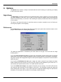
9. Options ........................................................................................................................................................... 37
Night Vision.................................................................................................................................................................... 37
Preferences .................................................................................................................................................................... 37
Grayscale Palette and Standard Palette................................................................................................................. 38
Appendix A ........................................................................................................................................................ 39
-5-
Autostar IP Contents
Image Processing Basics........................................................................................................................................... 39
Bibliography ...................................................................................................................................................... 41
Glossary ............................................................................................................................................................. 42
-6-
Autostar IP
Introduction
Welcome to Meade Autostar IP astronomical image processing software. Now you can perform many of
the same image processing tasks that a professional astronomer would do on a large institutional
computer. With Meade Autostar IP you can:
•
Enhance high resolution images using advanced image processing techniques.
•
Determine stellar magnitudes directly from electronic images, and a number of other powerful
features.
A Note on Accuracy
Meade Autostar IP was designed to be extremely powerful and accurate. Many programs designed for
the PC have taken shortcuts to appear faster, but at the expense of accuracy! Not Meade Autostar IP! By
carefully coding each section of the program using 64 bit floating point numbers, Meade Autostar IP takes
full advantage of your computer to provide fast and accurate performance. This gives you the power and
accuracy that rivals main-frame computer performance.
System Requirements
The minimum system required to run Meade Autostar IP are as follows:
•
64 MB RAM.
•
Hard Disk with 20 Megabytes of free space.
•
An VGA or better adapter and compatible monitor.
•
Microsoft Windows 98SE or above.
•
A Microsoft compatible mouse.
Registering the Program
Please take the time to fill out and mail the Registration Card you received with Meade Autostar IP.
Registering Meade Autostar IP entitles you to the following additional benefits:
•
•
•
Meade 's technical support, if you have difficulty using Meade Autostar IP.
Automatic notification of upgrades or revisions to Meade Autostar IP.
Automatic notification when new images or data become available.
-7-
Autostar IP
1. Installation
Autostar IP is installed as part of Meade’s Autostar Suite. If you have not yet installed the Suite, consult
the quickstart instructions for the complete instructions.
Typcially, when the Autostar Suite CD ROM is inserted in your computer it will automatically begin the
install process. If your system has “autoplay” disabled, click on START, then click on RUN. When the run
dialog box appears, type
A:SETUP then press Enter.
The Setup program will prompt you for the desired drive and path in which to install the program and data
files. Then it will begin uncompressing the files from the distribution disks and copying them to the
appropriate locations on the Hard disk. Make sure you have at least 60 Megabytes of free space on the
destination drive.
Once the installation is complete, Meade Autostar IP will be ready to help you begin processing your own
images.
-8-
Autostar IP
2. Features
Tool Bar
Autostar IP's Tool Bar gives you immediate access to image files to perform complex image processing
with the click of a button.
Status Bar
Autostar IP's "live" Status Bar constantly updates the coordinate display of the image, and the pixel value
(Dn.) of the image, as well as the local time. The Status Bar can also be customized under the
Preferences command under the File menu.
Menu Bar
The familiar Windows Menu Bar gives you access to every function of Autostar IP. To access a drop down
menu file, either click with the mouse or press Alt and the letter underlined from the keyboard.
-9-
Autostar IP
3. File
The file menu contains a number of commands for opening and closing image files, and printing
images.
Open
The Open command from the File menu or the button of the Tool Bar allows you open either images or
spectrographs in any of the following formats:
TIFF
FITS
BMP
LNX
ST7
ST6
ST4
08B
- Tagged Image File Format (16bit grayscale)
- Flexible Information Transport System (8 or 16 bit or floating point grayscale)
- Windows Bitmap Format (8 bit grayscale, 256 color, or 24 bit color)
- Spectra Source Lynxx format (12 bit grayscale)
- Santa Barbara Instrument Group (16 bit grayscale)
- Santa Barbara Instrument Group (16 bit grayscale)
- Santa Barbara Instrument Group (8 bit grayscale)
- Raw (8 bit grayscale). Similar to ST4.
In addition there is a RAW format for reading unknown image formats.
Images may only be saved in TIFF, FITS or BMP formats.
To open a file:
- Select the desired format.
- Select the directory and filename from the list boxes
OR
- Enter the desired filename in the edit box.
If the filename is specified without an extension, a default extension will be automatically added to the
filename to reflect the current format. If the extension is provided, it will over-ride the current selection
-10-
Autostar IP
Regardless of the file type, the image data will be converted to 16 bit integer data. This assures that high
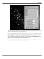
precession is maintained throughout image processing.
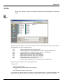
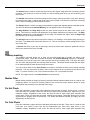
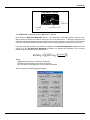
If the image is an RGB color image, you will be prompted as to which color plane you wish to load. The
following dialog will appear:
If you select Load As Color Image, the program will load all three color planes and display the image. As
an astronomical image processing program, Autostar IP is designed primarily to work on gray scale
images. Some of the more advance processing features will not be available when a color image is
loaded. If you wish to apply these more sophisticated techniques, load each plane individually, process it
and save it in a temporary file. These can later be combined back together to form the desired color
image.
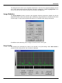
8 Bit versus 12 or 16 Bit or Floating Point Grayscale Images
When 12 or 16 bit or Floating point images are loaded, they need to be scaled down to 8 bits (256 gray
levels) for display, which is the maximum number of simultaneous gray shades that Windows can display
at one time. All of the image information is loaded an processed by the program, but it needs to be
scaled down to 256 gray levels for presentation. This scaling is called Prescaling. By default the program
is options are set to automatically prescale image data. At anytime you can manually prescale the data to
suite your taste.
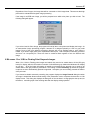
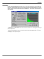
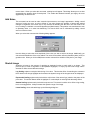
If you elected to disable automatic prescaling, the program displays the Image Prescale dialog box when
an image is loaded that allows manual setting of the parameters used to compress the data into an 8 bit
display format. This dialog box displays the histogram of the raw data in a large graph at the top and, at
the bottom, a smaller graph of the resulting data after the display scaling operation.
-11-
Autostar IP
Although the display shows only 256 levels, all of the image data are retained and processed by the
program. Whenever you perform a processing step, you are given an opportunity to rescale the display
data. The scale command, also allows you to rescale the image any time you desire.
When prescaling an image, a histogram is constructed that shows the distribution of the data contained in
the image. Normally the data is distributed in a rather narrow range of values which lends itself to scaling
to the 8 bit format. Once the histogram is constructed, the Threshold values of the data is calculated and
are used to set the scaling range. This gives a reasonable starting point for scaling most images. The
threshold values may be reset at any time by pressing the Threshold button.
Since the data is not evenly distributed, some fine-tuning of the limits is usually needed. This is
accomplished by using one of the predefined scaling options or by moving the red markers located under
the main histogram display. Generally, the best images are obtained with the markers set just at the high
and low edges of the important data. Values that are above the upper marker result in pure white pixels,
while those below result in pure black.
If the Std. Dev. button is depressed the Mean and Standard Deviation of the image are calculated. The
upper limit is set to the Mean plus 5 Standard Deviations, while the lower limit is set to the Mean minus 1
Standard Deviation.
The Min Max button sets the pointers to the extreme minimum and maximum values contained in the
image, while Full Scale sets the values to maximum and minimum values in the image.
If you are loading images from an RGB composite set of files, you may find it useful to use the same
scaling values for each of the individual images. This is easily accomplished by using the Use Previous
Scale Values button located at the bottom the dialog box. Since many astronomical images contain a
large amount of red light, you may want to load the red image first, scale it properly, then use the same
scaling values for both the green and blue images.
Close
Selecting Close will close the current file and remove its display window and any support windows, such
as the Histogram.
-12-
Autostar IP
Save As Fits Image
Displays the Save As dialog box and allows saving the current image data in a floating point FITS
formatted file. This method of saving insures that all of the information in the image is maintained. This is
the format recommended for keeping archival copies of your image data.
To save a file:
- Select the directory and filename from the list boxes
OR
- Enter the desired filename in the Edit box.
If the filename is specified without an extension, a default extension will be automatically added to the
filename to reflect the current format. If the extension is provided, it will over-ride the current selection
Export Display As
Saves the currently display image to a file. This function is only available if the current format type is TIFF,
FITS or BMP. This command will save the image as displayed on your computer as an 8 bit or 24 bit data
in the format you request. Saving images this way will allow you to save images ready for use in
documents, but will discard part of the original image data
To save a file:
- Select the desired format.
- Select the directory and filename from the list boxes
OR
- Enter the desired filename in the Edit box.
If the filename is specified without an extension, a default extension will be automatically added to the
filename to reflect the current format. If the extension is provided, it will over-ride the current selection
NOTE: All images are saved in the 8 bit versions of their respective format type, Some original
information may be lost.
Revert
The Revert command allows you to revert the image to the last saved version.
Print
Selecting the Print command or pressing the Print button from the Tool Bar prints the current image on
the system’s default printer. The image is scaled so that it completely fills the printing area of the paper in
the horizontal direction. The vertical scale is then chosen to preserve the original aspect ratio of the
image. Additional information pertaining to the image is also printed at the bottom of the page, below the
image.
Printer Setup
Displays the Printer Setup dialog box which allows the selection of any of the currently installed printers.
-13-
Autostar IP
To alter the print setting on a printer, highlight the printer in the Installed Printers window and select the
Setup button. The printer’s control dialog will open an allow you to modify its settings. Finally, if the
desired printer is not the systems Default Printer, user the Set Default Printer button to assign it as the
system default. Remember this change will also affect any other program started after the change has
been made.
The most common use of Printer Setup is to allow change between B&W or Color, or portrait and
landscape printing formats.
Page Setup
Selecting Page Setup allows you to customize the page to include headers, footers and set margins. You
can also select a border.
Exit
Shuts down Meade Autostar IP in an orderly fashion and returns to the Windows Manager. If there are
any modified files opened, you will be prompted to save those files.
-14-
Autostar IP
4.View
The View formatting section allows you to modify how the image data is presented on the display in a
number of ways. You can lighten or darken an image, change its contrast, or run a number of
sophisticated image processing functions to bring out or suppress subtle details contained in the image.
You can change the size of the image, tint its display palette or annotate it.
All of the functions in the View menu affect only the image display, not the actual image data.
To access the commands you can either click on View on the Menu Bar with the mouse, use the Alt key
and the appropriate underlined letter from the keyboard, or, when available, click on the appropriate button
from the Tool Bar.
Descriptions of the Image file commands from the Menu Bar appear below. The icon from the appropriate
button from the Tool Bar also appears next to the description for your reference.
Zoom Image Size
This command allows you to change the displayed size of the image. The image can be made larger or
smaller depending on your needs. This is generally used to allow an entire image to be displayed even if
the original image size exceeds the screen size.
The Fit Window button automatically scales the image so that all of the image can be displayed in the
current window regardless of the aspect ratio of the window. This means that one axis of the image may
not completely fill a portion of the window. You will notice that the Photometry cursor is constrained from
using the area outside the actual image area.
Scale
The Scale dialog allows you to modify the contrast and brightness of the image in a variety of ways.
Scaling is a two step process. The first step is to Prescale the image. This selects the range of data to be
mapped to the 256 available levels. The second step is final Scaling of the image.
Final scaling gives you a broad range of control. You change can be as simple as a straight linear scaling
or as complex as Histogram Equalization.
When a new image is loaded, the values in this dialog box are reset to their defaults. This allows you to
initially view the image in its un-altered state.
The graph displays the transformation that will be applied to the image values when the OK button is
depressed. The horizontal axis represents the input values to the transformation, while the vertical axis
represents the resulting values. Each axis is drawn to reflect the values of the current palette. With the
normal Linear transformation each input pixel corresponds to exactly the same output value, but only
when Contrast = 1.0 and Brightness = 0.
You can think of the Contrast and Brightness controls as the variables M and B in the equation of a
straight line,
Y = MX + B
where X is the input value, M is the slope of the line, B is the zero offset and Y is the resulting value. By
varying the Contrast control you can actually see the slope of the line changing. A steep slope results in
an image that quickly varies from black to white (high contrast), while a shallow slope (less than 1.0)
produces an image which is made up mainly of gray values. Setting the Contrast to a negative value
produces a negative image.
-15-
Autostar IP
Setting the Brightness control to values greater than zero brightens the image, while values less than
zero will darken it. Generally, you must use both the contrast and brightness controls together to achieve
the desired results.
The Linear function sets a straight line transformation that resets the contrast and brightness values to
1.0 and 0.0 respectively.
The Dynamic function analyzes the image for its lightest and darkest values (excluding pure black and
white) then sets up a linear transformation with the contrast and brightness adjusted to provide a full range
image. This is useful on images that are over or underexposed, or those that have poor contrast.
The Exponential function sets a non-linear transformation and resets both contrast and brightness. The
resulting exponential curve produces images that have lower contrast in the dark areas and higher
contrast in the light areas. This is useful for bringing out detail in the central regions of galaxies or
nebulae.
The Logarithmic function produces a curve that is the inverse of the Exponential. It increases the
contrast in the dark areas while lowering it in the bright areas. This helps to enhance the detail in the faint
arms of a galaxy.
The most complex transformation is Histogram Equalization.
Its purpose is
transformation curve that shows the maximum amount of detail in the image in all
accomplished by building a Histogram of the image (counting the number of pixels at
level), then constructing a curve that tries to equalize the number of pixels in each
brightness levels.
to construct a
areas. This is
each brightness
of the resulting
The maximum number of resulting levels can be set using the scroll bar, a greater number of steps
generally produces a smoother image. This value must be set before the Histogram Equalization button
is pressed. The maximum value is seldom reached since the equalization process greatly reduces the
number of initial gray levels. The default value of 128 is useful in the majority of cases since most images
tend to equalize to fewer than 64 steps.
Histogram Equalization is useful in almost all images, but remember that the resulting curve is far from
linear, so that further quantitative analysis (e.g., Magnitude determination) is impossible.
The Posterize function produces a stair stepped curve that can reduce the number of displayed values to
the predefined settings. By setting the number of steps with the scroll bar, depressing the Posterize
button displays the resulting curve and resets the contrast and brightness values. This feature is most
-16-
Autostar IP
useful for delineating areas of similar brightness to enhance the overall shape of an object such as a
comet or nebula.
Before committing to the scaling function that you have selected, you can Preview the image by pressing
the Preview button, you then have the option to select OK , Cancel , or try another scaling function.
Palettes
The Palettes dialog box allows you to modify the original palette of the image or to change the palette to
completely different sets of colors
The pushbuttons at the top of the dialog box loads a new palette and resets the positions of the Start
Color and Width scroll bars.
The Original button resets the palette to the values that were contained in the original image
The 16 Color button loads the standard 16 colors into the palette. This is useful on VGA systems that are
running in 16 color mode. The normal hardware palette values in VGA only support 3 shades of gray, but,
by using the 16 Color palette and selecting the Grayscale Palette from the Options menu, a full
grayscale of 16 colors can be used. This option changes ALL colors on the display (including all other
windows) while in a standard VGA 16 color mode!
The 16 Spectrum button builds a set of 16 colors that smoothly transition from Black, Blue, Green, Red
and ending with White. The appearance of this palette varies depending on the current video driver.
The 256 Gray button constructs a unique grayscale palette that emulates a full 256 color grayscale. The
standard Extended or Super VGA 256 color modes only support 64 different shades of gray. Using this
new palette results in a smoother image compared to the 64 shades palette. This is accomplished by
using color values that vary slightly from the pure gray colors. These off-color values are used to fill-in the
steps between the 64 pure gray values. If the Night Vision feature is active the 256 Gray button
becomes 256 Red which allows the image to be displayed in red to preserve your night vision.
The 256 Spectrum button constructs a 256 color palette that smoothly transitions from Black, Blue,
Green, Red and ends with White. This palette is especially useful for bringing out subtle detail in the
image.
NOTE: The 256 color palettes, when used in a 16 color mode, will display dithered colors that approximate
the actual values. Their appearance in the image may differ greatly depending on the 16 color driver that
is currently in use.
Red, Green, Blue, and Yellow buttons construct single color pallet that terminate in white.
-17-
Autostar IP
The Pseudo button constructs a pallet that contains red, green, and blue values for a generic 8 bit color
image.
There are two scroll bars on either side of the palette display. The uppermost scroll bar changes the
starting color of the palette, while the lower one changes the width of the palette. Moving the upper scroll
bar to the right has the effect of shifting the colors to the right, moving to the left moves the colors to the
left. The lower scroll bar allows the current palette values to be expanded or compressed. Moving the
lower scroll bar to the right expands the color palette, moving it to the left, compresses it and allows up to
5 cycles of the palette.
NOTE: If the palette has been inverted using the Invert button, the action of these buttons may appear
reversed.
The Invert button swaps the colors in the palette end-for-end. This is useful when displaying negative
images (those that appear as dark subjects on a light background). The button text changes to Revert to
indicate that the displayed palette is reversed.
Contour
The contour function allows you to perform an isophote analysis of the current image. This is
accomplished by drawing contour lines over the existing image. The spacing of these lines is controlled
by the Contour Interval value. For example, if the interval is set to 16, then a contour line will be drawn at
pixel value 16, 32, 48, etc.. This function is useful when trying to determine the shape of any diffuse
object such as a comet or galaxy. Using the Posterize function in the Image Scale utility will provide an
alternate method that is also useful when determining the shape of an object.
The contour process begins by building an Unsharp Mask of the current image. This is a smoothed
(blurred) version of the original image. Then the contouring algorithm is run using the smoothed image.
The resulting contour lines are then drawn over the current image. To vary the effect of the contouring,
the Region Size parameter can be changed to any desired value, a low value (3 or 4) gives a very ragged
contour line, a large value (11 or 12) provides a smooth contour. The default value of 7 is useful in most
images. You may need to experiment with different values to get the correct response for any given
image.
Blink
The Blink command allows you to easily detect differences between two images by rapidly displaying first
the image, then the other image. When the command is first executed, it first displays each of the images
and saves a special copy of each image in memory. It then begins a high-speed toggle of the images
using the special copies. The command may be terminated at any time by hitting the Stop button.
This command is especially useful for detecting changes in brightness or position of objects from one
image to the next.
To use, load an image from the Open command from the File menu then choose the Blink command from
the Image menu. Load the image to be blinked from the Select File option and click on Start. You can
then control the Offset Adjust (x/y position of the two images) and the Rate Adjust (blinking speed) in real
time.
Note: The images can be of different size images of different orientation.
-18-
Autostar IP
5.Tools
The Tools section allows you to examine the image data a number of ways. You can examine the image
header information, magnify close up sections of the image, view brightness distribution or examine
individual pixels.
All of the functions in the Tool menu are for analysis and do not affect only the image display, or image
data.
To access the commands you can either click on Tools on the Menu Bar with the mouse, use the Alt key
and the appropriate underlined letter from the keyboard, or, when available, click on the appropriate button
from the Tool Bar.
Descriptions of the Tool commands from the Menu Bar appear below. The icon from the appropriate
button from the Tool Bar also appears next to the description for your reference.
Coordinates
The Coordinates function displays a modeless dialog box that continuously shows the current
coordinates of the cursor while it is positioned over the image. The value of the pixel under the cursor is
also displayed and is updated as the cursor moves.
The pixel value may be displayed in three different formats: the 8 bit integer display value, the scaled
floating point value or the 16 bit unprocessed value. The 16 bit format is only available for 12 or 16 bit
images when the 16 bit data is resident. The mode can be chosen by selecting either the Integer, Real,
or Unprocessed button located at the bottom of the dialog box. See the Image Prescale function for
details on keeping the 16 bit data resident.
The coordinate dialog box must be active if you wish to make distance measurements from the image.
The Dist. field will display the distance value after the Set Distance Ref. function has been selected from
the Image Utilities dialog box.
Histogram
Displays a bar graph of the number of pixels in each of the 256 colors or shades of gray. The graph is
automatically scaled, and displayed in a logarithmic format.
The Max field at the top of the display indicates the maximum number of pixels contained in any of the
colors. The background grid is logarithmically scaled. The lower group of 10 lines indicate the values
from 1 to 10, the next group indicate the range from 10 to 100, the next group is 100 to 1000, and so on.
The histogram is automatically updated whenever the image values have been modified.
Magnifier
The Magnifier allows you to zoom into any portion of the display to observe small details. If an image is
displayed when the magnifier is turned on, the default starting location is the center of the image,
otherwise it uses the center of the client area of the main window. A new area can be selected by moving
the cursor onto the magnifier's
window, depressing the left mouse button, then, while still holding the left button, move to the desired
area.
The magnification factor can be changed by moving the scroll bar located on the right side of the magnifier
window. The magnification range is 1.0 to 32.0 in steps of 0.1. The default magnification is 4.0.
The size and location of the magnifier window can be modified using the standard methods.
-19-
Autostar IP
Information
Displays general data about the current image, such as, size, scale factors, date of image, location, etc..
Most of this data is a permanent part of the image and can be found in the headers of the various formats.
Only the size and bits per pixel values are saved in the BMP format. The FITS and TIFF formats save all
of the information.
The Scale Factor and Zero Offset fields contain the factors used to convert the image from the orignal
data to an 8 bit image.
The View FITS Header option allows you to determine the information file contained within a FITS image.
Also displayed is the image's histogram.
-20-
Autostar IP
6.Process
The Processing section allows you to modify the actual image a number of ways using advanced image
processing commands. Since the commands change the actual image data, this menu section features
an UNDO command that will allow you to restore the image data to the its state prior to the previous
command.
To access the Process commands you can either click on Process on the Menu Bar with the mouse, use
the Alt key and the appropriate underlined letter from the keyboard, or, when available, click on the
appropriate button from the Tool Bar.
Many of the image processing functions also allow for a preview so that you have the option to choose a
different variation of the function , choose OK, or to Cancel the function. The functions that offer the
Preview option are: Merge, Convolution Filters, Unsharp Masking, and RGB merge.
Descriptions of the Processing commands from the Menu Bar appear below. The icon from the
appropriate button from the Tool Bar also appears next to the description for your reference.
Undo
Resets the image variables to its previous values and re-displays the image. You can only 'Undo' the last
operation that affected the image data.
Calibrate
Select Bias Frames, Dark Frames, or Flat Field Frames for calibrating the image that is currently loaded
and displayed. Each of the three calibration types can be used singly or in combination.
Merge
The Merge Image command allows y you to select an image from the Merge File to perform a Merge
Function. You can select; Add, Subtract, Average, Median Combine, Multiply, Divide, And, Or, and
Exclusive Or functions. There is also the option to select x/y offsets, and Scale Factors of the Image File
and Merge File. (For a straight add or subtract both of these Scale Factor values should be set to 1.0.)
Correct Column Defect
Perfect solid state image sensors are difficult to make. Often units are produced that have one or more
columns that do not work correctly. These engineering grade sensors are often used in commercial CCD
cameras. The processing command allows you to replace a defective imager column with the average of
the two adjacent columns. When the command is selected a dialog box will prompt you to enter the
number of the defective column. Once this is done and confirmed, the column is replaced.
Flip Image
The currently displayed image may be flipped either vertically or horizontally. This allows the image to be
shown in its actual orientation if the telescope or camera system causes the image to appear inverted.
The Vertical and Horizontal flipping function may also be used in combination.
Rotate Image
The currently displayed image can be rotated in steps of either +90 degrees (counter-clockwise) or -90
degrees (clockwise) using the Rotate Image command.
Rotate Image must physically move the image data from one axis to the other. This changes the
orientation of the image in memory, therefore, subsequent buffer functions, such as merging, may not
-21-
Autostar IP
function properly. To preclude these problems, the contents of the buffers are destroyed before the
rotation takes place. You should then copy the rotated image into the desired buffer(s). After the
command is complete, the newly rotated image is automatically copied into Buffer A.
Resample
The Resample command changes the actual size of the image. This allows you to make an image larger
or smaller. Unlike Resizing which only affects the display, this command actually manipulates the image
data make it a new size. When you select this command, the following dialog appears:
To change the size of the image, just enter the new dimensions desired. If the Preserve Aspect Ratio
switch is set, Any time you enter either the width or height, the other number will be adjusted to perserve
the aspect of the image. With the switch off, you can maker changes that will alter the aspect ratio of the
final image. When you click on OK, the image will be modified.
Remember, when you reduce the size of the image, information will be lost.
Convolution Filters
The Convolution Filter dialog box displays the kernel values of the current convolution filter and allows
you to select from a list of pre-defined kernels or to enter your own values. See the Appendix for a
description of image convolution.
-22-
Autostar IP
The Normal button constructs a filter that does not alter the original image when the convolution process
is started. This allows you to reset the kernel to a normal starting point when you are constructing your
own kernels.
The Smooth button builds a kernel that subtly blurs the image, reducing the effect of any noise that may
be present in the image. Lowering the value of the center number in the kernel increases the smoothing
effect. While increasing the value reduces the effect.
The Sharpen button is useful in bringing out the details in images that originally appear somewhat blurred.
This effect is different than Unsharp Masking, but can appear similar in some images.
The Edge Enhance and Edge Only kernels are quite similar except for the value at the center of the
kernel. Their effect is to enhance the appearance of any edges (transitions) from light to dark. The Edge
Enhance maintains the overall appearance of the image, but modifies the edges, while the Edge Only
filter displays only the edge modifications.
The Average button merely sets all of the kernel values to 1.0 resulting in a 5x5 pixel average (blurring) of
the image. The Clear button sets all the values to 0.0. This can be used to set the starting values in your
own custom filter.
To Preview the effect of your filter on the image, click the preview button. Adjust the parameter until you
achieve the desired effect, then click OK.
Unsharp masking
This powerful command allows you to bring out the subtle detail that is normally not visible in the
unprocessed image. When this command is selected, the Unsharp Masking dialog box is displayed.
This allows you to set the region size used to produce the blurred unsharp mask. The larger the region
size, the more unsharp (blurrier) the resulting mask becomes. This allows details smaller than the region
to be enhanced after the mask and the image are merged.
You can try other values for the Scale Factors to increase or decrease the effect of the unsharp masking
technique. The only requirement is that the value for the image must be 1 greater than the value for the
mask. Try values such as: 5,4 or 6,5 to increase the effect, or 2,1 to decrease the effect.
NOTE: The original values of the Scale Factors are left untouched.
Median Filter
Median filtering modifies an image by replacing each pixel with the median (middle value) of it and all of its
neighboring pixels. It is useful for removing random noise, and some column defects. Works on single
pixel artifacts and smoothing out a generally noisy image.
Fix Hot Pixels
Even after calibration, images often have individual pixels that are too bright. These can be a result of
read noise from your camera, cosmic rays that hit your imager during the exposures, slight errors in your
calibration images. Regardless of the cause, this filter will look for these single pixel anomalies and
remove them. When you select this command, a dialog box will appear. This dialog allows you to set how
aggressively the program hunts for bad pixels. The smaller the threshold number you supply, the more
aggressively, the filter will act.
Fix Cold Pixels
Even after calibration, images often have individual pixels that are too dark. These can be a result of read
noise from your camera, cosmic rays that hit contaminated your dark frams, slight errors in your
calibration images. Regardless of the cause, this filter will look for these single pixel anomalies and
-23-
Autostar IP
remove them. When you select this command, a dialog box will appear. This dialog allows you to set how
aggressively the program hunts for bad pixels. The smaller the threshold number you supply, the more
aggressively, the filter will act.
Add Noise
This command can be used to make cosmetic improvement to an image’s appearance. Adding a small
amount of noise can cover up minor defects. It can also disguse the problem of areas with gradual
changes in brightness; the human eye is very effective at detecting the shift from one color level to the
next, resulting in a banded or contoured appearance (Mach bands). This problem can sometimes be seen
on planetary limbs, or in solar limb darkening. This visual effect can be eliminated by adding a small
amount of random noise.
When you select this command the following dialog appears:
Use this dialog to select the mean amplitude of the noise you wish to add to the image. Additionally, you
can select the distribution of the noise added. The noise can be wither uniformly distribute (white) noise, or
gausian noise. When you click on OK, these random values will be added to each pixel in your image.
Stretch Image
Stretching a image is the process of applying an algebraic function to each pixel in an image. This
process can be used to emphasis or de-emphasize highlights, or simply clip and scale image values.
Autostar IP offers several different scalings:
Log Scaling replaces each pixel with the log of its value. This has the effect of stretching the contrast to
favor details in the image highlights and increases the dynamic range of the image that can be displayed.
Exponential Scaling replace each pixel with the e (the base of the natural logs) raised to the power of the
pixel value. This stretch flattens detail in highlights. It is also helpful in reducing limb darkening effects.
Gamma Scaling replaces each pixel with its square root. This stretch is similar in its effect to log scaling,
but is not as aggressive. It helps increase the dynamic range of an image.
Linear Scaling, when selected brings up the following dialog box:
-24-
Autostar IP
Linear scaling performs the following transformation:
Final Pixel = (Pixel – Min.Value) * Scale Factor
If the Final Pixel is greater than Max. Value, the Final Pixel is assigned the Max. Value.
RGB Merge
The RGB Merge command produces a full color image by combining three separate grayscale images,
one exposed through a red filter, another exposed through a green filter, and the last exposed through a
blue filter If your system has 16 or 24 bit color modes, these images can be directly combined, otherwise
this is accomplished by analyzing all of the possible colors in the image, then using a proprietary algorithm
to choose the best colors to take full advantage of the 256 color system palette.
The RGB Merge command also allows you to modify the color balance of the final color image.
Increasing the scale factor for an individual color, increases the intensity of that color in the resulting
image, decreasing the scale factor decreases the overall intensity of that color in the image.
Each of the scale factors can be used separately or together to achieve any desired color balance. For
example, if the resulting image is too magenta, you might try lowering BOTH the red and blue scale
factors, or you may try increasing the green scale factor to achieve the same effect.
The scale factors may also be automatically determined by using the RGB Gray Balance function from
the Image Utilities dialog box. To automatically balance the colors in the image, first locate an area in the
image that should be white, or any neutral gray value such as a medium brightness star. Then draw a box
around the object by depressing the left mouse button and dragging the box to the desired size. When
the button is released, the Image Utilities dialog box will be displayed. If all three RGB buffers contain
valid images, the RGB Gray Balance item will be enabled. Upon selecting the RGB Gray Balance
function, the scale factors for each color will be determined and will automatically merge the buffers to
produce a new image. The resulting image will show your selected object as a shade of gray.
On 256 (8 bit) color systems, the Quantum Level field allows you to influence the behavior of the color
selection algorithm. If the resulting image contains a very large number of colors, lowering the Quantum
Level decreases the number of resulting colors. Similarly, raising the value increases the number of
colors, up to the maximum number of colors contained in the image. When the number of colors found in
the resulting image closely matches the number of colors used in the image, you will notice a marked
increase in the speed of the merging process.
-25-
Autostar IP
When the command is complete, the number of colors that were found and the number of colors used in
the resulting image are displayed. You should modify the number of Quantum Levels (in the RGB Merge
dialog box) so that the two values are fairly close together. Generally, finding 300 to 400 colors results in
the best image. Using a large number of colors results in an image that has a very small change in colors,
using fewer colors increases the color differences seen in the image
The resulting color image has its own unique palette, subsequent image processing, such as scaling,
generally gives poor results. You should first scale the individual red, green, or blue grayscale images,
then combine them using the RGB Merge command.
To preserve the color palette, the color image must be saved in the BMP format.
Frequently, many composite RGB images are not perfectly registered, the telescope may have moved
between the exposures. This results in one or more of the images being offset from the other images.
The Offsets {XE Image:Offsets} the X (horizontal) direction or the Y (vertical) direction one pixel at a time
for each of the Red, Green, and Blue image files.
After the image is first merged, you should examine some prominent part of the image using the
Magnifier. If color fringes are noticed over the entire image, one or more of the separate images needs
to be aligned with the others. Count the number of pixels that the images appear to be offset, then set the
value in the appropriate red, green or blue X or Y offset fields. When the images are re-merged, the new
offset values will be used.
If the images were taken from a telescope that was not properly Polar aligned, the resulting images may
also show some rotation from one image to the next, The RGB alignment may help reduce the effect
slightly, but cannot correct for the rotation.
The individual offsets may also be automatically determined by using the RGB Alignment function from
the Image Utilities dialog box. To automatically align the images, first locate an area in the image that
contains a well defined single object, such as a star. Then draw a box around the object by depressing
the left mouse button and dragging the box to the desired size. When the button is released, the Image
Utilities dialog box will be displayed. If all three RGB buffers contain valid images, the RGB Alignment
item will be enabled. Upon selecting the auto alignment function, the X and Y offsets for each image will
be determined and will automatically merge the buffers to produce a new image.
-26-
Autostar IP
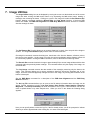
7. Image Utilities
The Image Utilities dialog box can be displayed by moving the cursor over the desired area of the current
image and either clicking the left mouse button or by depressing the left mouse button, drawing a
rectangle, then releasing the button. Clicking on a point in the image will enable the Set Distance Ref.
function, drawing a rectangle enables the Rescale Size and Crop Image functions. If the three RGB
buffers are loaded, the RGB Auto Alignment and RGB Gray Balance functions will also be available
after the rectangle is drawn.
The Set Distance Ref. function allows you to measure distances, in pixels, from one point in the image to
another. The image Coordinates display must be active to use this function.
Choosing this command, removes the dialog box, then draws a line from the distance reference point to
the current cursor position. As the cursor is moved, the current coordinates and the distance values will
be continuously updated. Clicking the left mouse button, turns-off the distance measuring feature.
The Rescale Size command scales the image to approximately fill the current image window with the data
contained within the previously drawn rectangle. This command affects only the display of the image, not
the actual data.
The Crop Image command removes the data outside of the rectangle, preserving only the data on the
inside. This command allows you to remove extraneous data from around the important part of your
image. Since this command physically changes the size of the image, any existing data contained in the
buffers is destroyed.
See the RGB Merge command for a description of the RGB Auto Alignment and the RGB Gray
Balance functions.
The Set Log File command allows you to name a text file where information about the image can be
written. Several operations including, List Pixel Values, Draw Profiles, Image Statitics, Determine
Magnitude, and Group Photometry can write information to the Log file. This information can then be
used in spread sheets or by other analysis tools. When you click on this button the following dialog
appears:
Here you can specify where to write the log file. If the file already exists, you will be prompted to indicate
whether you wish to append data to the existing file, or to erase it and start again.
-27-
Autostar IP
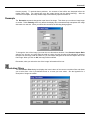
Set Reference Magnitude
To calculate the magnitude of any object in the current image, you must first select an object whose
magnitude is already known. Draw a selection box around the object. Then select the Set Reference
Magnitude function. The following dialog will appear.
All magnitude calculations in Meade Autostar IP are based on a technique called Aperture Photometry.
This method comparing the total energy inside a measurement radius around a target object with that
within the aperature of the reference object. Total energy is defined to be the sum of all pixels the
aperature less the average sky brightness times the number of pixels in the aperture. The sky
brighteness in determined by measuring the sky background in an annulus about the object. This dialog
allows you to select the size of the aperature and annulus for measurements.
Additionally, the aperture is centered on your target before the measure measurements are made. The
size of the box used to centroid your object for centering is also configurable in this dialog. Finally, if you
check the Auto Log Magnitudes box, all measurements are automatically written to the log file for export
to spread sheets or other analysis programs.
Determining Magnitude
To perform photometry, draw a box around the area that you wish to determine by moving the cursor to
the upper left corner of the region, depress and hold the left mouse button, then drag the opposite corner
of the box to the other side of the object. Release the button when you are satisfied with the appearance
of the photometry region cursor.
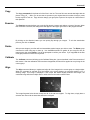
The Photometry region cursor has three main components: the Magnitude/Centroid area, the Pixel list
area, and the Profile line. The Magnitude/Centroid rectangle bounds the entire area used in the
magnitude and/or centroid calculations. This area can be as large as the entire image if desired. Finally,
the Profile line delineates the pixels that will be displayed when the Draw Profile function is selected.
-28-
Autostar IP
Photometry Cursor
Profile Line
Pixel List
Area
Mag/Centroid Area
The Utilities Box is displayed when the left button is released.
Now choose the Determine Magnitude function. You should pick a well defined object, such as a star,
whose values are below the maximum set by the size of the data format. A warning message will be
displayed if the selected region contains any pixels that are at the maximum. Erroneous values will result
if you use objects that contain these pixel values since the actual brightness of these pixels in unknown.
Using the previously set value of the reference magnitude, the Determine Magnitude calculates the total
energy as in the Set Reference Magnitude command, but displays the magnitude of the currently
selected region defined by the following equation:
RefMag +
(
5
100 ∗log
10
( RefTotal
))
Total
Where,
RefMag is the previously set reference magnitude
RefTotal is the total energy in the reference aperture.
and Total is the total energy in the currently selected aperture.
After a moment the following dialog will appear:
-29-
Autostar IP
This dialog show the result of your magnitude determination. Not only is the magnitude displayed, but the
error of the measurement and other pertenant information is displayed. If Auto Log Magnitudes is not
set, you can still write the results to the log file by clicking on the Log button.
Image Statistics
The Image Statistics function is similar to the magnitude functions except that it displays only the the
statistical information about the selected region. Additionally, Image statistics are calculate over the whole
selected region, not just within the photometric aperture. An example result dialog is show below:
Click OK to dismiss the dialog. Click on Log to write these values to the log file.
Draw Profile
The selection box determines the values to be included in the profile dialog. When Draw Profile is
selected a Profile dialog similar to the one below is displayed.
-30-
Autostar IP
If the Line Profile button is selects, the diagonal line drawn through the Photometry Cursor indicates
which pixels will be graphed by the Draw Profile command. Other choices are the summation of the
rows, average of the rows, summation of the columns or average of the columns. If the Scaled Values
box is checked, the screen’s display values are used, otherwise the image pixel values are used to
generate the profile.
When this function is selected, a linearly scaled graph will be drawn which is automatically scaled to
display the entire range of the pixel values along the line. The left side of the graph displays the pixels
values at the start of the cursor box. Since you may draw the box in any orientation, you must keep track
of the starting point.
The profile graph is useful for viewing spectrographic data, or for viewing trends in the data, such as limb
darkening in a planetary image.
To write out the profile as a table of values to the log file, click on the Write to Log button.
List Pixel Values
The List Pixel Values function displays the values of the pixels contained within the smaller box located in
one corner of the overall cursor rectangle. The maximum size of the pixel list area is 25x25 pixels. If the
cursor rectangle is smaller than 25x25 pixels you will see only one rectangle. You will then see only those
pixels contained within the entire region.
The pixel values displayed are the actual image pixel values. If you click on the Print button, these values
will be printed on the default system printer. If you click on Write to Log, the pixel values for the whole
selected area, not just the 25x25 box, will be written to the log file in this tabular format. This allows you to
export large areas of the image to spread sheets or other software analysis tools.
One common use of these exported files is to create 3-D surface plots in spread sheets such as Excel or
Star Office.
-31-
Autostar IP
Edit Log File
The Edit Log File command opens the current log file for editing with either wordpad or notepad. This
allows you to add annotations to you log file as you work though and image, or to remove unwanted data
that may accidentally have been written to the file.
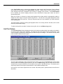
The sample below shows what a typical log file might look like.
-32-
Autostar IP
8. Group Operations
The Group Operations menu contains commands that will allow you to process groups of files
simulaneously. There are many tasks such as calibration, image combination, alignment and filtering
where the same task may need to be done to a whole collection of images. The ability to operate on
groups of images is one of the keys to making Autostar Image Processing the most convenient Windows
image processing system.
Group Edit
Selecting the Group Edit command opens the group editing dialog window that allows you to manage
your image group. An Image group is nothing more than a list of files. This dialog allows you to add and
delete file names from the list.
To erase the list and start over, select Clear List. To add images to the list, select Add Images. This will
open a standard windows explorer file selection dialog box. You can use this box to select a single file to
be added to the list, or by holding down the Shift or Ctrl key when clicking, you can select multiple images
to be added to your group.
When you are satisfied with your selection, click Open to add them to the current group.
-33-
Autostar IP
Copy
The Copy command will duplicate all of the files in the list. The new file have named that begin with the
phrase "Copy_Of_”. Often, you do not want to operate on your original data, this makes it easy to create
backup copies to work on. Copy will also change your group list to point to the copies as a side effect of
this operation.
Examine
The Examine command allows you to quickly flip through, inspect and analyze a group of images. When
this command is selected, the dialog below will appear in the upper right corner of the program window.
By clicking on the direction buttons you can quickly flip through you images. To exit the examination
process, just click on Cancel.
Delete
After process images, you often will hve intermediate results images you wish to erase. The Delete group
command is a fast easy way to clean up. Use the Edit command to gather all you scrap files into an
image group, then select Delete. You will be prompted to confirm your delete. If you reply OK, all the files
in the group will be moved to the recycle bin.
Calibrate
The Calibrate command will bring up the Calbirate Dialog box, just as described in the Process section of
this manual. After the calibration files have been designated, the files will be applied to every image in the
current group.
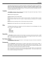
Align
The Align command allows you register and align all of the images in the current gourp to a single object.
When the command is selected all of the images in the group together are summed together to for a
working image. This image is displayed. If the scope has drifted slightly between the images, the
combined image will show multiple stars or trails similar to the section shown below:
The image fragment below shows clearly how all of the star are trippled. To align them, simply draw a
selection box around all the stars that should be co-aligned.
-34-
Autostar IP
The program will go through all of the images an shift them so that they will be aligned on the select star.
After the the images have been aligned, a proof image will be created by averaging together all of the
images in your group and displaying the results. It may take a couple of interrations to get all the images
to line up if you are working in a crowded star field. The technique will work best if the alignment star is in
a relatively isolated portion of the image.
Combine
The Combine command is used to combine all of the images in the group into a single image. There are
several different combination methods available.
Sum adds all the images together.
Average averages all of the images together.
Median takes the middle value of all the images at each pixel location. This method will drop out cosmic
ray hits and other random noise from a group of images although the processing can be somewhat
lengthy.
Minimum takes the smallest pixel value of all the images at each pixel location.
Maximum takes the largest pixel value of all the images at each pixel location.
Filter
The Filter command allows you to apply any of the filter techniques found under Process to the entire
group of images. Filters available include:
Convolve
Median
Unsharp Mask
Fix Hot Pixels
Fix Cold Pixels
Normalize
The Normalize command processes all of the images in the group so that their mean value is 10,000
ADUs. This command is most commonly used to prescale sky or twilight flats before median combining
them to drop out stars, satellites and other transient effects.
Fix Column Defect
The Fix Column command, fixes bad columns in all the images of the group. If functions as described in
the Process section of this manual.
Photometry
The group Photometry command allows you to measure a large number of stars in group of images. It
makes variable star, extra-solar planet transit searches, asteroid rotation and comet study easy. In all of
these activities, you may have a large number of images of the same field of view taken at different times
where you wish to measure the same group of objects in each image.
When this command is selected the group photometry dialog will appear similar to the example shown
below. Additionally, the first image in your group will be displayed behind it. Select all the objects that you
wish to measure by drawing a box around them.
-35-
Autostar IP
The center coordinates of the locator boxes are shown in the window at the top of the dialog. Additionally,
you can change the aperture and annulus of measurement.
If you check the Recenter and Track box, each object will be recentered in each succeeding image. This
allows you compensate for slight shifts of the telescope between measurements,. Additionally, for aligned
images, it will allow you to track a comet or asteroid as it moves through the field of view.
Since it is likely you will be using this data in other program, chekcing the Columnar Format box will
output your results in a simple to export columnar format in the log file.
When you have made all of your selections, click on proceed and the program will perform all
measurements on all images a write the results to your log file.
-36-
Autostar IP
9. Options
The Options menu contains a variety of commands that are useful in setting up or optimizing your display
for the current task at hand.
Night Vision
The Night Vision command changes all of the standard system colors to shades of red to help maintain
your eyes adaptation to the dark. This is useful if you are using the program during actual observing
session in the observatory or in the field. After selecting this option you should also lower the brightness
on your monitor.
The status of the night vision option is saved from session to session, remember to turn it off when you
are using the program in normal lighting.
Preferences
Under Preferences you can configure the status bar and set up key option that control the behavior of the
program. When selected, the following dialog appears:
The status bar appearance is controlled by the check boxes on the right. On the left are the image
handling options.
If you check Auto Contrast On Load, the program will automatically prescale images with the indicated
method when a new image is loaded. Enabling this option smooths operation of the program considerably.
Only when working with merging RGB images or when special displays are required is it recommended to
diable this option.
If you check the Fit Window On Load option, images are sized to exactly file your display area when
loaded. Enabling this option assures you will see all your image on load regardless of your screen size. To
see full detail you may still need to zoom in or out with from the main menu.
If you check 24 Bit Color Images, the program will assume you are running a 16 to 32 bit color card on
your computer and will process all color images as 24 bit color. This will greatly increase the speed and
ease of dealing with color images. If you need to output 8 bit compressed palette images for rapid internet
download, or if your system has only and 8 bit color display, disable this option.
-37-
Autostar IP
Grayscale Palette
and Standard Palette
The Grayscale Palette and Standard Palette commands are used together to optimize your systems'
ability to display gray scale images. If you are running in a standard VGA display mode, these commands
will be enabled. Since these commands are not required in other display modes, they will appear
disabled.
The standard VGA mode allows only 16 simultaneous colors, with this limitation in mind, Windows
requires that these colors be set to the standards 'pure' colors, e.g. red, green, blue, magenta, etc., this
provides only two gray values plus black and white. To improve you capability of viewing the high
resolution B/W images, Epoch 2000 re-programs the hardware registers on the VGA board to display 16
gray values instead of 16 'pure' colors. By selecting the standard 16 color palette in the Image, Palette
menu when the Grayscale Palette is active, you will be able to view the images in 16 shades of gray
NOTE: The Grayscale Palette function removes all colors from the display leaving only shades of gray.
Make sure you restore the regular colors by selecting the Standard Palette before you run other color
intensive applications.
-38-
Autostar IP Appendix
39
Appendix A
Image Processing Basics
Image processing allows you to modify the appearance of an image by applying various types of filters,
scaling options or transformations. The simplest type of processing is linear scaling. With linear scaling,
one pixel from the source image is multiplied by a scale factor, then an offset term is added. The original
pixel value is then replaced with the resulting value. This process is repeated on each pixel in the image.
The contrast and brightness of the image can be controlled by varying the scale factor (contrast) and the
offset value (brightness). You should attempt to set the contrast to a value that allows the full range of the
important parts of the image to fall on the sloping section of the transfer curve (see the Scale Image
function), then set the brightness so that the minimum pixel values appear black or very dark gray. The
following histogram and transfer graph illustrates the optimal contrast and brightness settings to give a
normal view of the image.
You may need to experiment to find the right settings for any given image. Sometimes it may be
necessary to scale different areas of the image using
Another useful image processing technique, convolution, allows you to enhance the appearance of an
image by 'filtering' the image data by either smoothing (low-pass filter) or sharpening (high-pass filter) or
combining parts of both types of filters.
This is accomplished by passing a convolution matrix, or kernel, over the entire image and replacing the
center pixel in the resulting matrix with the scaled sum of all of the other values. For example, if you
wanted to average each pixel with its adjacent neighbors the following kernel could be used.
11
11
11
1
1
1
Each pixel, including the center one, would be multiplied by 1, then the sum of each of these terms is
calculated. The result is then divided by the sum of each of the kernel values, in this case 9. Finally, the
-39-
Autostar IP Appendix
40
center pixel value is replaced with the new result. This process is then repeated for every pixel in the
image.
There are many different kernels that you can create that give various results. Meade Autostar IP
provides several basic kernels that provide the most common functions, but feel free to experiment.
There are a number of image processing books available that will describe other types of kernels.
-40-
Autostar IP Appendix
Bibliography
William K. Pratt, Digital Image Processing, second edition, John Wiley & Sons, Inc., New York, 1991
-41-
41
Index
42
Glossary
absolute magnitude - the apparent magnitude an object would have if it were moved to a distance of 10
parsecs.
angular diameter - the apparent diameter of an object expressed in angular measure i.e., deg, min, sec.
aperture - the diameter of the objective lens or primary mirror of a telescope.
apparent magnitude - the observed brightness of an object without any correction for distance.
astrometry - the branch of astronomy concerned with the precise measurement of positions and motions
of celestial objects.
coma - an optical defect that affects only image details away from the center of the field of view causing
stars to appear flared, like tiny comets pointing inward from the edge of the field.
focal length - the distance from the lens or mirror to the focal point.
focus - the oint in an optical system where all the image components are brought together.
-42-