Download Campbell DC112 Operator`s manual

21X MICROLOGGER
OPERATOR’S MANUAL
REVISION: 3/96
COPYRIGHT (c) 1984-1996 CAMPBELL SCIENTIFIC, INC.
This is a blank page.
WARRANTY AND ASSISTANCE
The 21X MICROLOGGER is warranted by CAMPBELL SCIENTIFIC, INC. to be free from defects in
materials and workmanship under normal use and service for thirty-six (36) months from date of shipment
unless specified otherwise. Batteries have no warranty. CAMPBELL SCIENTIFIC, INC.'s obligation under
this warranty is limited to repairing or replacing (at CAMPBELL SCIENTIFIC, INC.'s option) defective
products. The customer shall assume all costs of removing, reinstalling, and shipping defective products
to CAMPBELL SCIENTIFIC, INC. CAMPBELL SCIENTIFIC, INC. will return such products by surface
carrier prepaid. This warranty shall not apply to any CAMPBELL SCIENTIFIC, INC. products which have
been subjected to modification, misuse, neglect, accidents of nature, or shipping damage. This warranty
is in lieu of all other warranties, expressed or implied, including warranties of merchantability or fitness for
a particular purpose. CAMPBELL SCIENTIFIC, INC. is not liable for special, indirect, incidental, or
consequential damages.
Products may not be returned without prior authorization. To obtain a Returned Materials Authorization
(RMA), contact CAMPBELL SCIENTIFIC, INC., phone (435) 753-2342. After an applications engineer
determines the nature of the problem, an RMA number will be issued. Please write this number clearly on
the outside of the shipping container. CAMPBELL SCIENTIFIC's shipping address is:
CAMPBELL SCIENTIFIC, INC.
RMA#_____
815 West 1800 North
Logan, Utah 84321-1784
CAMPBELL SCIENTIFIC, INC. does not accept collect calls.
Non-warranty products returned for repair should be accompanied by a purchase order to cover the repair.
This is a blank page.
21X OPERATOR'S MANUAL
TABLE OF CONTENTS
PAGE
WARRANTY AND ASSISTANCE
SELECTED OPERATING DETAILS ............................................................................................. V
CAUTIONARY NOTES ..................................................................................................................... VI
OVERVIEW
OV1. PHYSICAL DESCRIPTION
OV1.1
OV1.2
OV1.3
OV1.4
OV1.5
OV1.6
Analog Inputs ...................................................................................................................... OV-2
Switched Excitation Outputs ............................................................................................... OV-3
Continuous Analog Outputs ................................................................................................ OV-3
Digital Control Ports ............................................................................................................ OV-3
Pulse Count Inputs .............................................................................................................. OV-3
12 Volts and Ground ........................................................................................................... OV-3
OV2. MEMORY AND PROGRAMMING CONCEPTS
OV2.1
OV2.2
OV2.3
Internal Memory .................................................................................................................. OV-3
21X Instruction Types ......................................................................................................... OV-5
Program Tables and the Execution and Output Intervals ................................................... OV-5
OV3. PROGRAMMING THE 21X
OV3.1
OV3.2
OV3.3
OV3.4
OV3.5
Functional Modes ................................................................................................................ OV-7
Key Definition ...................................................................................................................... OV-7
Programming Sequence ..................................................................................................... OV-7
Instruction Format ............................................................................................................... OV-8
Entering a Program ............................................................................................................. OV-8
OV4. PROGRAMMING EXAMPLES
OV4.1
OV4.2
OV4.3
Sample Program 1 .............................................................................................................. OV-9
Editing an Existing Program .............................................................................................. OV-11
Sample Program 2 ............................................................................................................ OV-12
OV5. DATA RETRIEVAL OPTIONS ................................................................................... OV-15
OV6. SPECIFICATIONS ......................................................................................................... OV-18
i
TABLE OF CONTENTS
PROGRAMMING
PAGE
1.
1.1
1.2
1.3
1.4
1.5
1.6
1.7
1.8
2.
2.1
2.2
2.3
3.
3.1
3.2
3.3
3.4
3.5
3.6
3.7
3.8
3.9
3.10
FUNCTIONAL MODES
Program Tables - *1, *2, and *3 Modes ................................................................................. 1-1
Setting and Displaying the Clock - *5 Mode ........................................................................... 1-2
Displaying and Altering Input Memory or Flags - *6 Mode ..................................................... 1-2
Compiling and Logging Data - *0 Mode ................................................................................. 1-3
Memory Allocation - *A........................................................................................................... 1-4
Memory Testing and System Status - *B Mode ..................................................................... 1-6
C Mode - Security................................................................................................................... 1-6
*D Mode - Save or Load Program .......................................................................................... 1-7
INTERNAL DATA STORAGE
Final Storage Areas, Output Arrays, and Memory Pointers ................................................... 2-1
Data Output Format and Range Limits .................................................................................. 2-2
Displaying Stored Data on Keyboard/Display - *7 Mode ........................................................ 2-3
INSTRUCTION SET BASICS
Parameter Data Types ........................................................................................................... 3-1
Repetitions ............................................................................................................................. 3-1
Entering Negative Numbers ................................................................................................... 3-1
Indexing Input Locations ........................................................................................................ 3-1
Voltage Range and Overrange Detection .............................................................................. 3-2
Output Processing.................................................................................................................. 3-2
Use of Flags: Output and Program Control........................................................................... 3-3
Program Control Logical Constructions ................................................................................. 3-4
Instruction Memory and Execution Time................................................................................ 3-6
Error Codes ............................................................................................................................ 3-9
DATA RETRIEVAL/COMMUNICATION
4.
4.1
4.2
4.3
4.4
4.5
5.
5.1
5.2
6.
6.1
6.2
6.3
6.4
6.5
EXTERNAL STORAGE PERIPHERALS
On-Line Data Transfer - Instruction 96, *4 Mode ................................................................... 4-1
Manually Initiated Data Output - *8 and *9 Modes ................................................................. 4-2
Cassette Tape Option ............................................................................................................ 4-4
Storage Module (SM192/716) ................................................................................................ 4-6
Printer Output Formats........................................................................................................... 4-7
TELECOMMUNICATIONS
Telecommunications Commands .......................................................................................... 5-1
Remote Programming of the 21X .......................................................................................... 5-3
9 PIN SERIAL INPUT/OUTPUT
Pin Description ....................................................................................................................... 6-1
Enabling Peripherals .............................................................................................................. 6-2
Interrupting Data Transfer to Storage Peripherals ................................................................. 6-2
Telecommunications - Modem Peripherals............................................................................ 6-2
Interfacing with Computers, Terminals, and Printers ............................................................. 6-2
ii
TABLE OF CONTENTS
PROGRAMMING EXAMPLES
PAGE
7.
7.1
7.2
7.3
7.4
7.5
7.6
7.7
7.8
7.9
7.10
7.11
7.12
7.13
7.14
7.15
7.16
8.
8.1
8.2
8.3
8.4
8.5
8.6
8.7
8.8
MEASUREMENT PROGRAMMING EXAMPLES
Differential Voltage - LI200S Silicon Pyranometer ..................................................................7-1
Datalogger and Sensor with a Common External Power Supply............................................7-1
Thermocouple Temperatures Using 21X Reference ..............................................................7-2
Thermocouple Temperatures Using an External Reference Junction ....................................7-2
107 Temperature Probe ..........................................................................................................7-3
207 Temperature and RH Probe.............................................................................................7-3
Anemometer with Photochopper Output .................................................................................7-4
Tipping Bucket Rain Gauge with Long Leads .........................................................................7-4
100 ohm PRT in 4 Wire Half Bridge........................................................................................7-5
100 ohm PRT in 3 Wire Half Bridge........................................................................................7-6
100 ohm PRT in 4 Wire Full Bridge ........................................................................................7-7
Pressure Transducer - 4 Wire Full Bridge ..............................................................................7-8
Lysimeter - 6 Wire Full Bridge.................................................................................................7-9
227 Gypsum Soil Moisture Block ..........................................................................................7-10
Nonlinear Thermistor in Half Bridge (CSI Model 101)...........................................................7-11
Measuring 107 Temperature Probe with 60Hz Rejection .....................................................7-12
PROCESSING AND PROGRAM CONTROL EXAMPLES
Computation of Running Average ...........................................................................................8-1
Rainfall Intensity ......................................................................................................................8-2
Using Control Ports and Loop to Run AM416 Multiplexer.......................................................8-3
SUB 1 Minute Output Interval Synched to Real Time .............................................................8-5
SDM-AO4 Analog Output Multiplexer to Strip Chart ...............................................................8-5
Converting 0-360 Wind Direction Output to 0-540 for Strip Chart...........................................8-7
Covariance Correlation Programming Example......................................................................8-8
Fast Fourier Transform Examples ........................................................................................8-11
INSTRUCTIONS
9.
INPUT/OUTPUT INSTRUCTIONS..................................................................................9-1
10.
PROCESSING INSTRUCTIONS ...................................................................................10-1
11.
OUTPUT PROCESSING INSTRUCTIONS................................................................11-1
12.
PROGRAM CONTROL INSTRUCTIONS ..................................................................12-1
MEASUREMENTS
13. 21X MEASUREMENTS
13.1
13.2
13.3
13.4
13.5
13.6
Fast and Slow Measurement Sequence ...............................................................................13-1
Single-Ended and Differential Voltage Measurements .........................................................13-1
The Effect of Sensor Lead Length on the Signal Settling Time ............................................13-3
Thermocouple Measurements ............................................................................................13-10
Bridge Resistance Measurements ......................................................................................13-15
Resistance Measurements Requiring AC Excitation ..........................................................13-19
iii
TABLE OF CONTENTS
INSTALLATION
PAGE
14. INSTALLATION AND MAINTENANCE
14.1
14.2
14.3
14.4
14.5
14.6
14.7
14.8
14.9
14.10
Protection From the Environment ........................................................................................ 14-1
Power Requirements............................................................................................................ 14-2
21X Power Supplies ............................................................................................................. 14-3
Solar Panels ......................................................................................................................... 14-4
Direct Battery Connection to the 21X ................................................................................... 14-4
Vehicle Power Supply Connections ..................................................................................... 14-4
Use of Digital Control Ports for Switching Relays ................................................................ 14-5
Grounding............................................................................................................................. 14-5
Maintenance......................................................................................................................... 14-6
Calibration Procedures......................................................................................................... 14-6
APPENDICES
A.
GLOSSARY .......................................................................................................................... A-1
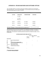
B.
PROM SIGNATURES AND SOFTWARE OPTIONS ............................................... B-1
C.
BINARY TELECOMMUNICATIONS
C.1
C.2
C.3
Telecommunications Command With Binary Responses......................................................C-1
Final Storage Format .............................................................................................................C-3
Generation of Signature .........................................................................................................C-4
D.
ASCII TABLE........................................................................................................................D-1
E.
CHANGING RAM OR PROM CHIPS
E.1
E.2
E.3
F.
Disassembly of 21X ............................................................................................................... E-1
Installing New RAM Chips...................................................................................................... E-1
Changing PROM Chips .......................................................................................................... E-2
DOCUMENTATION FOR SPECIAL SOFTWARE .................................................... F-1
LIST OF TABLES .......................................................................................................................... LT-1
LIST OF FIGURES ........................................................................................................................ LF-1
INDEX ................................................................................................................................................... I-1
iv
SELECTED OPERATING DETAILS
1. Storing Data - Data is stored in Final
Storage only by Output Processing
Instructions and only when the Output Flag
is set. (Sections OV2 and OV3.3)
PROMs are available which have different
combinations of instructions. Appendix B
describes the options available and gives
the signatures of the current PROMS.
2. Storing Date and Time Date and time are
stored in Final Storage ONLY if the Real
Time Instruction 77 is used. (Section 11)
3. Data Transfer - On-line data transfer from
Final Storage to peripherals (tape, printer,
Storage Module, etc.) occurs only if enabled
with Instruction 96 in the datalogger
program or in the *4 Mode. (Section 4.1)
9. Significant changes in the current PROM
release (OSX-0.1, OSX-1.1, and OSX-2.1)
include:
INSTRUCTIONS
Case Statement (83 & 93, Section 12)
Arc Tangent (66 Section 10)
Wind Vector (69 replaces 76, Section 11)
4. Final Storage Resolution - All Input Storage
values are displayed (*6 mode) as high
resolution with a maximum value of 99999.
However, the default resolution for data
stored in Final Storage is low resolution,
maximum value of 6999. Results
exceeding 6999 are stored as 6999 unless
Instruction 78 is used to store the values in
Final Storage as high resolution values.
(Sections 2.2.1 and 11)
5. Floating Point Format - The computations
performed in the 21X use floating point
arithmetic. CSI's 4 byte floating point
numbers contain a 23 bit binary mantissa
and a 6 bit binary exponent. The largest
and smallest numbers that can be stored
18
-19
and processed are 9 x 10 and 1 x 10 ,
respectively. (Section 2.2.2)
Serial Output has an option to send a file mark
to a Storage Module (96, Section 12)
Low Pass Filter: on the first execution after
compiling, the input value is used for the filtered
result
Commands to set, toggle and pulse ports are
now available for Program Control Instructions
(Section 12)
Revision 3 of the above PROMS includes the
capability to sense status(0 V low, 5 V high) on
the high side of a differential channel
(Instruction 91, Section 12).
FEATURES
Ports can now be manually toggled from the
keyboard or TERM (PC208 software)
6. Erasing Final Storage Data in Final Storage
can be erased without altering the program
by repartitioning memory in the *A Mode.
(Section 1.5.2)
The *B Mode now displays PROM version and
revision, execution overruns, and accumulated
error 8s in addition to signatures.
7. ALL memory can be erased and the 21X
completely reset by entering 978 for the
number of bytes left in Program Memory.
(Section 1.5.2)
The capability of transferring programs via
cassette tape is no longer supported in the
standard PROM options.
8. The set of instructions available in the 21X
is determined by the PROM (Programmable
Read Only Memory) that it is equipped with.
v
This is a blank page.
CAUTIONARY NOTES
1. Damage will occur to the analog input
circuitry if voltages in excess of ±16 V are
applied for a sustained period. Voltages in
excess of ±8V will cause errors and
possible overranging on other analog input
channels.
3. The sealed lead acid batteries used with the
21XL are permanently damaged if
discharged below 11.76 V. The cells are
rated at a 2.5 Ahr capacity but experience a
slow discharge even in storage. It is
advisable to maintain a continuous charge
on the 21XL battery pack, whether in
operation or storage (Section 14).
2. There are frequent references in this
manual to Storage Modules. The Storage
Modules referred to are the SM192 and
SM716. The old SM16 and SM64 Storage
Modules cannot perform many of the
functions available with the SM192 and
SM716.
vi
This is a blank page.
21X MICROLOGGER OVERVIEW
The 21X Micrologger combines precision measurement with processing and control capability in a single
battery operated system.
Campbell Scientific, Inc. provides three documents to aid in understanding and operating the 21X:
1.
2.
3.
This Overview
The 21X Operator's Manual
The 21X Prompt Sheet
This Overview introduces the concepts required to take advantage of the 21X's capabilities. Hands-on
programming examples start in Section OV4. Working with a 21X will help the learning process, so don't
just read the examples, turn on the 21X and do them. If you want to start this minute, go ahead and try
the examples, then come back and read the rest of the Overview.
The sections of the Operator's Manual which should be read to complete a basic understanding of the
21X operation are the Programming Sections 1-3, the portions of the data retrieval Sections 4 and 5
appropriate to the method(s) you are using (see OV5), and Section 14 which covers installation and
maintenance.
Section 6 covers details of serial communications. Sections 7 and 8 contain programming examples.
Sections 9-12 have detailed descriptions of the programming instructions, and Section 13 goes into
detail on the 21X measurement procedures.
The Prompt Sheet is an abbreviated description of the programming instructions. Once familiar with the
21X, it is possible to program it using only the Prompt Sheet as a reference, consulting the manual if
further detail is needed.
Read the Selected Operating Details and Cautionary Notes at the front of the Manual before using the
21X.
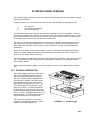
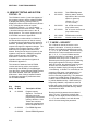
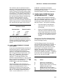
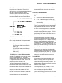
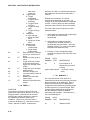
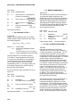
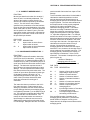
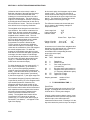
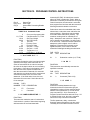
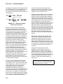
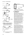
OV1. PHYSICAL DESCRIPTION
The 21X Micrologger is shown in Figure OV1-1.
The 21X is powered with 8 alkaline "D" cells
and has only the power switch on the base.
The 21XL is powered with rechargeable lead
acid cells and, in addition to the power switch,
has a charger input plug and an LED which
lights when the charging circuit is active. The
21XL should always be connected to a solar
panel or AC charger. The lead acid batteries
provide backup in event of a power failure but
are permanently damaged if their voltage drops
below 11.76 volts. Campbell Scientific does not
warrant batteries. The battery base is the only
difference between the 21X and the 21XL.
The 16 character keyboard is used to enter
programs, commands and data; these can be
viewed on the 8 digit display (LCD).
FIGURE OV1-1. 21X Micrologger
OV-1
21X MICROLOGGER OVERVIEW
The 9-pin serial I/O port provides connection to
data storage peripherals, such as the
SM192/716 Storage Module or RC35 Cassette
Recorder, and provides serial communication to
computer or modem devices for data transfer or
remote programming (Section 6). This 9 pin port
does NOT have the same pin configuration as
the 9 pin serial ports currently used on many
personal computers. An SC32A is required to
interface the 21X to a RS232 serial port
(Section 6).
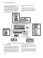
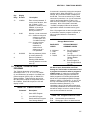
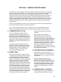
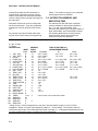
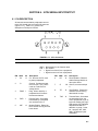
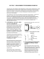
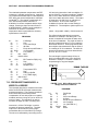
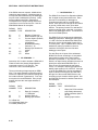
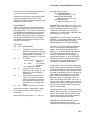
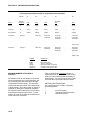
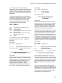
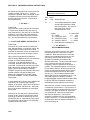
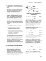
The panel also contains two terminal strips
which are used for sensor inputs, excitation,
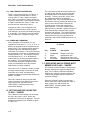
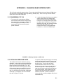
control outputs, etc. Figure OV1-2 shows the
21X panel and the associated programming
instructions.
FIGURE OV1-2. 21X Wiring Panel and Associated Programming Instructions
OV1.1 ANALOG INPUTS
The terminals in the upper strip are for analog
inputs. The numbering on the terminals refers to
the differential channels; i.e., the voltage on the
HI input is measured with respect to the voltage
on the LOW input. When making single-ended
measurements either the HI or the LOW channel
may be used independently to measure the
voltage with respect to the 21X ground. SingleOV-2
ended channels are numbered sequentially, e.g.
the HI and LOW sides of differential channel 2
are single-ended channels 3 and 4, respectively
(Section 13.2).
The analog input terminal strip has an insulated
cover to reduce temperature gradients across
the input terminals. The cover is required for
accurate thermocouple measurements (Section
13.4).
21X MICROLOGGER OVERVIEW
OV1.2 SWITCHED EXCITATION OUTPUTS
The first four numbered terminals on the lower
terminal strip are the SWITCHED EXCITATION
channels. These supply programmable
excitation voltages for resistive bridge
measurements. The excitation channels are
only switched on during the measurement.
OV1.3 CONTINUOUS ANALOG OUTPUTS
The two Continuous Analog Output (CAO)
channels supply continuous output voltages,
under program control, for use with strip charts,
X-Y plotters, or proportional controllers.
OV1.4 DIGITAL CONTROL PORTS
The six DIGITAL CONTROL PORTS (0 or 5
volt states) allow on-off control of external
devices. These control ports have a very
limited current output (5 mA) and are used to
switch solid state devices which in turn provide
power to relay coils (Section 14.4).
OV1.5 PULSE COUNT INPUTS
The four PULSE COUNT INPUTS measure
contact closure, low level AC, or high frequency
pulse signals.
OV1.6 12 VOLTS AND GROUND
The +12 volt terminal provides a direct
connection to the 21X power supply. The +12
and ground terminals can be used to connect
an external 12 volt battery to the 21X to
maintain system power while changing internal
batteries or to provide power for extended
periods in the field.
OV2. MEMORY AND PROGRAMMING
CONCEPTS
The 21X must be programmed before it will
make any measurements. A program consists
of a group of instructions entered into a program
table. The program table is given an execution
interval which determines how frequently that
table is executed. When the table is executed,
the instructions are executed in sequence from
beginning to end. After executing the table, the
21X waits the remainder of the execution
interval and then executes the table again
starting at the beginning.
The interval at which the table is executed will
generally determine the interval at which the
sensors are measured. The interval at which
data are stored is separate and may range from
samples every execution interval to processed
summaries output hourly, daily, or on longer or
irregular intervals.
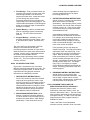
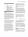
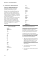
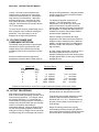
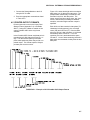
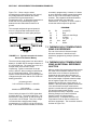
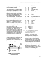
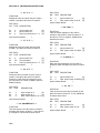
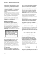
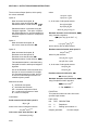
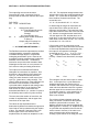
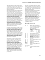
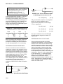
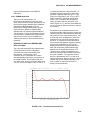
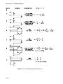
Figure OV2-1 represents the measurement,
processing, and data storage sequence in the
21X and shows the types of instructions used to
accomplish these tasks.
OV2.1 INTERNAL MEMORY
The 21X has 40,960 bytes of Random Access
Memory (RAM), divided into five areas. The
five areas of RAM are:
1. Input Storage - Input Storage holds the
results of measurements or calculations.
The *6 Mode is used to view Input Storage
locations to check current sensor readings
or calculated values. Input Storage defaults
to 28 locations. Additional locations can be
assigned using the *A Mode.
2. Intermediate Storage - Certain Processing
Instructions and most of the Output
Processing Instructions maintain
intermediate results in Intermediate
Storage. Intermediate storage is
automatically accessed by the Instructions
and cannot be accessed by the user. The
default allocation is 64 locations. The
number of locations can be changed using
the *A Mode.
OV-3
21X MICROLOGGER OVERVIEW
Sensor
Control
INPUT/OUTPUT
INSTRUCTIONS
Specify the conversion of a sensor signal to a
data value and store it in Input Storage.
Programmable entries specify:
(1) the measurement type
(2) the number of channels to measure
(3) the input voltage range
(4) the Input Storage Location
(5) the sensor calibration constants used to
convert the sensor output to engineering
units
I/O Instructions also control analog outputs
and digital control ports.
PROCESSING INSTRUCTIONS
INPUT STORAGE
Holds the results of measurements or
calculations in user specified locations. The
value in a location is written over each time a
new measurement or calculation stores data to
the locations.
Perform calculations with values in Input
Storage. Results are returned to Input
Storage. Arithmetic, transcendental and
polynomial functions are included.
INTERMEDIATE STORAGE
OUTPUT PROCESSING
INSTRUCTIONS
Perform calculations over time on the values
updated in Input Storage. Summaries for Final
Storage are generated when a Program
Control Instruction sets the Output Flag in
response to time or events. Results may be
redirected to Input Storage for further
processing. Examples include sums,
averages, max/min, standard deviation,
histograms, etc.
Provides temporary storage for
intermediate calculations required by the
OUTPUT PROCESSING
INSTRUCTIONS; for example, sums,
cross products, comparative values, etc.
Output Flag set high
FINAL STORAGE
Final results from OUTPUT PROCESSING
INSTRUCTIONS are stored here for on-line or
interrogated transfer to external devices
(Figure OV5.1-1). The newest data are stored
over the oldest in a ring memory.
FIGURE OV2-1. Instruction Types and Storage Areas
OV-4
21X MICROLOGGER OVERVIEW
3. Final Storage - Final, processed values are
stored here for transfer to printer, tape, solid
state Storage Module or for retrieval via
telecommunication links. Values are stored
in Final Storage only by the Output
Processing Instructions and only when the
Output Flag is set in the users program. The
19,296 locations allocated to Final Storage at
power up is reduced if Input or Intermediate
Storage is increased.
4. System Memory - used for overhead tasks
such as compiling programs, transferring
data, etc. The user cannot access this
memory.
5. Program Memory - available for user
programs entered in Program Tables 1 and
2, and Subroutine Table 3. (Sections OV3,
1.1)
The use of the Input, Intermediate, and Final
Storage in the measurement and data
processing sequence is shown in Figure OV2-1.
While the total size of these three areas remains
constant, memory may be reallocated between
the areas to accommodate different
measurement and processing needs (*A Mode,
Section 1.5). The size of system and program
memory, are fixed.
OV2.2 21X INSTRUCTION TYPES
Figure OV2.1 illustrates the use of the three
different instruction types which act on data. The
fourth type, Program Control, is used to control
output times and vary program execution.
Instructions are identified by numbers.
1. INPUT/OUTPUT INSTRUCTIONS (126,101-104, Section 9) control the terminal
strip inputs and outputs (the sensor is the
source, Figure OV1-2), storing the results in
Input Storage (destination). Multiplier and
offset parameters allow conversion of linear
signals into engineering units. The Control
Ports and Continuous Analog Outputs are
also addressed with I/O Instructions.
2. PROCESSING INSTRUCTIONS (30-66,
Section 10) perform numerical operations
on values located in Input Storage (source)
and store the results back in Input Storage
(destination). These instructions can be
used to develop high level algorithms to
process measurements prior to Output
Processing (Section 10).
3. OUTPUT PROCESSING INSTRUCTIONS
(69-82, Section 11) are the only instructions
which store data in Final Storage
(destination). Input Storage (source) values
are processed over time to obtain averages,
maxima, minima, etc. There are two types
of processing done by Output Instructions:
Intermediate and Final.
Intermediate processing normally takes
place each time the instruction is executed.
For example, when the Average Instruction
is executed, it adds the values from the
input locations being averaged to running
totals in Intermediate Storage. It also keeps
track of the number of samples.
Final processing occurs only when the
Output Flag is high. The Output Processing
Instructions check the Output Flag. If the
flag is high, final values are calculated and
output. With the Average, accumulated
totals are divided by the number of samples
and the resulting averages sent to Final
Storage. Intermediate locations are zeroed
and the process starts over. The Output
Flag, Flag 0, is set high by a Program
Control Instruction which must precede the
Output Processing Instructions in the user
entered program.
4. PROGRAM CONTROL INSTRUCTIONS
(85-98, Section 12) are used for logic
decisions and conditional statements. They
can set flags, compare values or times,
execute loops, call subroutines, conditionally
execute portions of the program, etc.
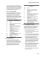
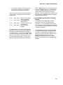
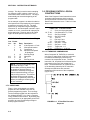
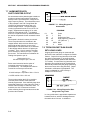
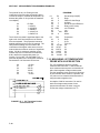
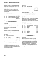
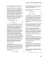
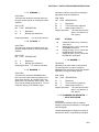
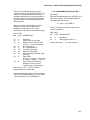
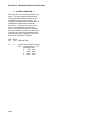
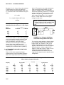
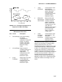
OV2.3 PROGRAM TABLES AND THE
EXECUTION AND OUTPUT INTERVALS
Programs are entered in Tables 1 and 2.
Subroutines, called from Tables 1 and 2, are
entered in Subroutine Table 3. The size of each
table is flexible, limited only by the total amount
of program memory. If Table 1 is the only table
programmed, the entire program memory is
available for Table 1.
Table 1 and Table 2 have independent
execution intervals, entered in units of seconds
OV-5
21X MICROLOGGER OVERVIEW
Table 1.
Execute every x sec.
0.0125 < x < 6553
Instructions are executed
sequentially in the order
they are entered in the
table. One complete pass
through the table is made
each execution interval
unless program control
instructions are used to
loop or branch execution.
Normal Order:
MEASURE
PROCESS
CHECK OUTPUT COND.
OUTPUT PROCESSING
Table 2.
Execute every y sec.
0.1 < y < 6553
Table 2 is used if there is a
need to measure and
process data on a separate
interval from that in Table
1.
Table 3.
Subroutines
A subroutine is executed
only when called from
Table 1 or 2.
Subroutine Label
Instructions
End
Subroutine Label
Instructions
End
Subroutine Label
Instructions
End
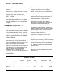
FIGURE OV2-2. Program and Subroutine Tables
with an allowable range of 0.0125 to 6553
seconds. Intervals shorter than 0.1 seconds
are allowed only in Table 1. Subroutine Table 3
has no execution interval; subroutines are only
executed when called from Table 1 or 2.
OV2.3.1 THE EXECUTION INTERVAL
The execution interval specifies how often the
program in the table is executed, which is
usually determined by how often the sensors are
to be measured. Unless two different
measurement rates are needed, use only one
table. A program table is executed sequentially
starting with the first instruction in the table and
proceeding to the end of the table.
Each instruction in the table requires a finite
time to execute. If the execution interval is less
than the time required to process the table, the
21X overruns the execution interval, finishes
processing the table and waits for the next
execution interval before initiating the table.
When an overrun occurs, decimal points are
shown on either side of the G on the display in
the LOG mode (*0). Overruns and table priority
are discussed in Section 1.1.
OV-6
OV2.3.2 THE OUTPUT INTERVAL
The interval at which output occurs is
independent from the execution interval, other
than the fact that it must occur when the table is
executed (i.e., a table cannot have a 10 minute
execution interval and output every 15 minutes).
A single program table can have many different
output intervals and conditions, each with a
unique data set (output array). Program Control
Instructions are used to set the Output Flag
which determines when output occurs. The
Output Processing Instructions which follow the
instruction setting the Output Flag determine the
data output and its sequence. Each additional
output array is created by another Program
Control Instruction setting the Output Flag high
in response to an output condition, followed by
Output Processing Instructions defining the data
set to output.
OV3. PROGRAMMING THE 21X
A program is created by keying it directly into the
datalogger or on a PC using the PC208
Datalogger Support Software program EDLOG.
This manual describes direct interaction with the
21X MICROLOGGER OVERVIEW
21X. Work through the direct programming
examples in this overview before using EDLOG
and you will have the basics of 21X operation as
well as an appreciation for the help provided by
the software. Section OV3.5 describes options
for loading the program into the 21X.
OV3.1 FUNCTIONAL MODES
User interaction with the 21X is broken into
different functional MODES, (e.g., programming
the measurements and output, setting time,
manually initiating a block data transfer to
Storage Module, etc.). The modes are referred
to as Star (*) Modes since they are accessed by
first keying *, then the mode number or letter.
Table OV3-1 lists the 21X Modes.
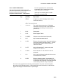
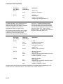
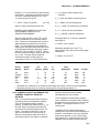
TABLE OV3-1. * Mode Summary
Key
Mode
*0
*1
*2
*3
*4
LOG data and indicate active Tables
Program Table 1
Program Table 2
Program Table 3, subroutines only
Enable/disable tape and/or printer
output
Display/set real time clock
Display/alter Input Storage data,
toggle flags
Display Final Storage data
Final Storage data transfer to
cassette tape
Final Storage data transfer to printer
Memory allocation/reset
Signature test/PROM version
Security
Save/load Program
*5
*6
*7
*8
*9
*A
*B
*C
*D
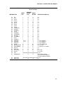
OV3.2 KEY DEFINITION
Keys and key sequences have specific
functions when using the 21X keyboard or a
terminal/computer in the remote keyboard state
(Section 5). Table OV3-2 lists these functions.
In some cases, the exact action of a key
depends on the mode the 21X is in and is
described with the mode in the manual.
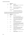
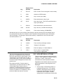
TABLE OV3-2. Key Description/Editing
Functions
Key
Action
0-9
*
Key numeric entries into display
Enter Mode (followed by Mode
Number)
Enter/Advance
Back up
Change the sign of a number or index
an input location to loop counter
Enter the decimal point
Clear the rightmost digit keyed into
the display
Advance to next instruction in
program table (*1, *2, *3) or to next
output array in Final Storage (*7)
Back up to previous instruction in
program table or to previous output
array in Final Storage
Delete entire instruction
A
B
C
D
#
#A
#B
#D
OV3.3 PROGRAMMING SEQUENCE
In routine applications, sensor signals are
measured, processed over some time interval,
and the results are stored in Final Storage. A
generalized programming sequence is:
1. Enter the execution interval, determined by
the desired sensor scan rate.
2. Enter the Input/Output Instructions required
to measure the sensors.
3. Enter any Processing Instructions required
to get the data ready for Output Processing.
4. Enter a Program Control Instruction to test
the output condition and Set the Output
Flag when the condition is met. For
example, use Instruction 92 to output based
on time, 86 to output each time the table is
executed, and 88 or 89 to compare input
values. This instruction must precede the
Output Processing Instructions.
5. Enter the Output Processing Instructions to
store processed data in Final Storage. The
order in which the data are stored is
determined by the order of the Output
Processing Instructions in the table.
6. Repeat steps 4 and 5 for output on different
intervals or conditions.
OV-7
21X MICROLOGGER OVERVIEW
OV3.4 INSTRUCTION FORMAT
Instructions are identified by an instruction
number. Each instruction has a number of
parameters that give the 21X the information it
needs to execute the instruction.
The 21X Prompt Sheet has the instruction
numbers in red, with the parameters briefly
listed in columns following the description.
Some parameters are footnoted with further
description under the "Instruction Option Codes"
heading.
For example, Instruction 73 stores the
maximum value that occurred in an Input
Storage Location over the output interval. The
instruction has three parameters (1)
REPetitionS, the number of sequential Input
Storage locations on which to find maxima, (2)
TIME, an option of storing the time of
occurrence with the maximum value, and (3)
LOC the first Input Storage Location operated
on by the Maximum Instruction. The codes for
the TIME parameter are listed in the "Instruction
Option Codes".
The repetitions parameter specifies how many
times an instruction's function is to be repeated.
For example, four 107 thermistor probes, wired
to single-ended channels 1 through 4, are
measured using a single Instruction 11, Temp107, with four repetitions. Parameter 2
specifies the input channel of the first thermistor
(channel 1) and parameter 4 specifies the Input
Storage Location in which to store
measurements from the first thermistor. If
Location 5 were used, the temperature of the
thermistor on channel 1 would be stored in Input
Location 5, the temperature from channel 2 in
Input Location 6, etc.
Detailed descriptions of the instructions are
given in Sections 9-12.
OV3.5 ENTERING A PROGRAM
Programs are entered into the 21X in one of
four ways:
1. Keyed in using the 21X keyboard.
2. Loaded from a pre-recorded listing using
the *D Mode. There are 2 types of
storage/input:
OV-8
a. Stored on disk/sent from computer
(PC208 software TERM and EDLOG).
b. Stored/loaded from SM192/716 Storage
Module
3. Loaded from Storage Module or internal
PROM (special software) upon power-up.
A program is created by keying it directly into
the datalogger as described in the following
Section, or on a PC using the PC208
Datalogger Support Software.
EDLOG and TERM are PC208 Software
programs used to develop and send programs
to the 21X. EDLOG is a prompting editor for
writing and documenting programs for Campbell
Scientific dataloggers. Program files developed
with EDLOG can be downloaded directly to the
21X using TERM. TERM supports
communication via direct wire, telephone, or
Radio Frequency (RF).
Programs on disk can be copied to a Storage
Module with SMCOM. Using the *D Mode to
save or load a program from a Storage Module
is described in Section 1.8.
If the SM192/716 Storage Module is connected
when the 21X is powered-up the 21X will
automatically load program number 8, provided
that a program 8 is loaded in the Storage
Module (Section 1.8).
It is also possible (with special software) to
create a PROM (Programmable Read Only
Memory) that contains a datalogger program.
With this PROM installed in the datalogger, the
program will automatically be loaded and run
when the datalogger is powered-up, requiring
only that the clock be set.
OV4. PROGRAMMING EXAMPLES
We will start with a simple programming
example. There is a brief explanation of each
step to help you follow the logic. When the
example uses an instruction, find it on the
Prompt Sheet and follow through the description
of the parameters. Using the Prompt Sheet
while going through these examples will help
you become familiar with its format. Sections 912 have more detailed descriptions of the
instructions.
21X MICROLOGGER OVERVIEW
OV4.1 SAMPLE PROGRAM 1
The 21X has a thermistor built into the input
panel that measures the panel temperature and
provides a reference for thermocouple
temperature measurements. In this example
the 21X is programmed to read the panel
temperature every 5 seconds and send the
results directly to Final Storage.
TURN ON THE POWER SWITCH AND
PROCEED AS INDICATED
Key
Display Shows
(ID:Data)
Explanation
--
HELLO
On power-up, the 21X displays "hello" while it
checks the memory.
after a few seconds delay
--
11:111111
The result of the memory check. Each digit
represents a memory socket on the CPU board.
1's indicate good memory, 0's bad memory
(Section 1.5).
*
00:00
Select mode.
1
01:00
Enter Program Table 1.
A
01:0.0000
Advance to execution interval (seconds).
5
01:5
Key 5 second execution interval.
A
01:P00
Enter the 5 second execution interval and advance
to the first program instruction location. The 21X
prompts with a P when it is time to enter an
instruction number.
17
01:P17
Key in I/O Instruction 17, measure the panel
temperature in degrees C.
A
01:0000
Enter Instruction 17 and advance to the first
parameter.
1
01:1
Key in the Input Storage location in which to store
the measurement; location 1.
A
02:P00
Enter the location number. Note that the 21X
knows how many parameters are associated with
an instruction and will prompt for a new instruction
number when parameter entry is completed.
The 21X is now programmed to read the panel temperature every five seconds and place
the reading in Input Storage location 1. Before adding any more instructions, we will start the
program and display the measurement in Input Storage.
OV-9
21X MICROLOGGER OVERVIEW
Key
Display Shows
(ID:Data)
Explanation
*0
:LOG 1
Exit Table 1, enter *0 mode to compile table and
begin measurements.
*6
06:0000
Enter *6 mode to view Input Storage.
A
01:21.234
Advance to Input Storage location 1. Panel
temperature is 21.234oC.
Wait a few seconds:
01:21.423
The measurement will be updated every 5
seconds when a new measurement is made.
At this point the 21X is measuring the temperature every 5 seconds and sending the value
to Input Storage. No data are being saved. The next step is to have the 21X send each
reading to Final Storage. (Remember the Output Flag must be set first.)
OV-10
Key
Display Shows
(ID:Data)
Explanation
*1
01:00
Exit *6 mode. Enter Program Table 1.
2A
02:P00
Advance to 2nd instruction location; this is where
we left off. Note how we jumped to the 2nd
instruction instead of just advancing by keying A.
86
02:P86
86 is the DO instruction; a Program Control
Instruction which unconditionally executes a
command.
A
01:00
Enter instruction and advance to the first
parameter specifying the command.
10
01:10
10 is the command to set Flag 0, the Output Flag.
The command codes are listed in the Instruction
Option Codes for Instructions 86-92 on the Prompt
Sheet and in Table 12.1-2.
A
03:P00
Enter the command and advance to third program
instruction location.
70
03:P70
The Output Processing Instruction, SAMPLE,
transfers values from Input Storage to Final
Storage when the Output Flag is set.
A
01:00
Enter 70 and advance to first parameter specifying
the repetitions.
1
01:1
There is only one value to sample so only one
repetition is entered.
21X MICROLOGGER OVERVIEW
Key
Display Shows
(ID:Data)
Explanation
A
02:0000
Enter repetition and advance to the second
parameter which specifies the first Input Storage
location to sample.
1
02:1
Input Storage location 1, where the panel
temperature is stored.
A
04:P00
Enter location and advance to fourth instruction
location. Note that a value is not entered into
memory until A is keyed. If *0 was keyed after the
1 in the previous step, the location would not be
entered and would remain 0.
*0
:LOG 1
Exit Table 1, enter *0 mode, compile program, and
log data.
The 21X is now programmed to measure the panel temperature every 5 seconds and send each
reading to Final Storage. Values in Final Storage can be viewed using the *7 Mode (Section 2.3):
Key
Display Shows
(ID:Data)
Explanation
*7
07: 13.000
Enter *7 Mode. The Data Storage Pointer (DSP) is
displayed showing the next available Final Storage
Location (location 13 in this example).
A
01: 0102
Advance to the first value, the output array
Identifier (ID). The ID indicates the Output Flag
was set in Table 1 by the second instruction
(Section 2.1).
A
02: 21.23
Advance to the first temperature stored. Note that
there are only 4 digits displayed (low resolution)
while the readings in Input Storage displayed 5
digits (Section 2.2 and Inst. 78).
A
01: 0102
Advance to the next output array. Same output
array ID.
A
02: 21.42
Advance to 2nd stored temp.
*0
:LOG 1
Change to *0 Mode.
In the above example, no time information is stored with the data. In the second example,
Instruction 77 is used to save the time of the measurements.
OV4.2 EDITING AN EXISTING PROGRAM
When editing an existing program in the 21X,
entering a new instruction inserts the
instruction; entering a new value for an
instruction parameter replaces the previous
value.
To insert an instruction, enter the program table
and advance to the position where the
instruction is to be inserted (i.e., P in the data
portion of the display) key in the instruction
number, and then key A. The new instruction
OV-11
21X MICROLOGGER OVERVIEW
will be inserted at that point in the table,
advance through and enter the parameters.
The Instruction that was at that point and all
instructions following it will be pushed down to
follow the inserted instruction.
An instruction is deleted by advancing to the
instruction number (P in display) and keying #D
(Table OV3-2).
value then key A. Note that the new value is not
entered until A is keyed.
The next example program uses the panel
temperature measurement but uses timed
intervals for output instead of every execution.
To get ready for the example, we will delete
Instructions 86 and 70.
To change the value entered for a parameter,
advance to parameter and key in the correct
Key
Display Shows
(ID:Data)
Explanation
: LOG1
21X is in *0 Mode
*1
01:00
Enter Program Table 1.
2A
02:P86
Jump to 2nd instruction in table; Instruction 86,
DO.
#D
02:P70
Delete Instruction 86. Second instruction is now
70.
#D
02:P00
Delete Instruction 70. Second instruction is now
vacant.
*0
:LOG1
Return to *0 Mode
OV4.3 SAMPLE PROGRAM 2
Our second example is more representative of
a data collection situation. This time the panel
temperature will be used as the reference
temperature for a type T (copper-constantan)
thermocouple (TC). Thermocouples measure
the temperature relative to their reference
junction temperature. To obtain the absolute
temperature, the reference junction temperature
must be known.
The 21X is shipped with a short thermocouple
wired to differential channel 5. The copper lead
is connected to the high input (H) and the
constantan lead is connected to the low input
(L). We'll read the sensor every 5 seconds, and
store one hour average temperatures along with
a daily maximum and minimum temperature
and the times at which they occur. The date
and time will also be stored with the data.
OV-12
Instruction 14 measures TC temperature with a
differential voltage measurement. The first
parameter is the number of times to repeat the
measurement. There is only one thermocouple,
so we enter a 1. If there were several TCs, they
could be wired to sequential input channels and
the number of TCs would be entered in
Parameter 1. The 21X would measure all of the
TCs.
Parameter 2 is the full scale voltage input range
to use when making the measurement. Type T
TC signals are very small, approximately
40µV/oC difference in temperature between the
measurement and reference junction. If we use
a range code of 1 (±5 mV full scale, slow
integration), the TC voltage will not exceed the
input range as long as the measurement
junction is within 125oC of the panel
temperature.
21X MICROLOGGER OVERVIEW
Parameter 3 specifies the channel on which to
make the first measurement. Parameter 6
specifies the Input Storage location in which to
store the first channel measurement. If multiple
repetitions are specified, measurements from
sequential channels are stored in adjacent input
locations beginning with the location specified in
Parameter 6. For Example, if there are 5
repetitions and the first measurement is stored
in location 3, the final measurement will be
stored in location 7.
Parameter 5 specifies the Input Storage
location in which to find the reference
temperature in this case location 1 where the
panel temperature is stored. Parameters 7 and
8 are the multiplier and offset which convert the
measurement to engineering units. The TC
instructions return the measurement in units of
oC
when a multiplier of 1 and an offset of 0 are
used.
The first example was explained one keystroke
at a time. Instead of listing each keystroke, the
following format shows the display after a value
is keyed in; the use of the A key to advance to
the next entry is not shown. This format is
similar to that used in the PC208 EDLOG
program.
If you have followed through sample program 1
and edited the program in OV4.2, your 21X
now has a 5 second execution interval and
Instruction 17 in Table 1. To continue with this
example you can simply advance (key A)
through the execution interval and Instruction 17
and check the entries against the following
listing. The new entry starts with the second
instruction in the table.
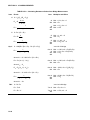
Sample Program 2
Instruction
(Loc.:Entry)
Parameter
(Par.#:Entry)
Description
*1
Enter Program Table 1
01:5
5 second execution interval
01:P17
01:1
Measure panel temperature
Store temp. in location 1
01:1
02:1
03:5
04:1
05:1
06:2
07:1
08:0
Measure thermocouple temp. (differential).
1 repetition.
Range code (5mV, slow).
Input channel of TC.
TC type: copper-constantan.
Reference temp is stored in location 1.
Store TC temp in location 2.
Multiplier of 1 (degrees C)
Offset of 0.
01:0
02:60
03:10
If Time
0 minutes into the interval.
60 minute interval.
Set Output Flag (Flag 0).
02:P14
03:P92
The 21X is programmed to measure the thermocouple temperature every 5 seconds. The If Time
Instruction, 92, sets the Output Flag at the beginning of each hour. Next, the instructions for time
and average are added.
OV-13
21X MICROLOGGER OVERVIEW
Instruction
(Loc.:Entry)
Parameter
(Par.#:Entry)
04:P77
01:10
05:P71
01:1
02:2
To obtain daily output, the If Time instruction is
again used to set the Output Flag and is
followed by the Output Instructions to store time
and the daily maximum and minimum
temperatures and the time each occurs.
Any Program Control Instruction which is used
to set the Output Flag high will set it low if the
conditions are not met for setting it high.
Instruction 92 above sets the Output Flag high
Instruction
(Loc.:Entry)
Parameter
(Par.#:Entry)
06:P92
Description
Output Time
Store hour and minute.
Average
One repetition.
Source of TC temps to be
averaged, Input Storage location 2.
every hour. The Output Instructions which
follow do not output every hour because they
are preceded by another Instruction 92 which
sets the Output Flag high at midnight (and sets
it low at any other time). This is a unique
feature of Flag 0. The Output Flag is set low at
the start of each table (Section 3.7).
Description
01:0
02:1440
03:10
If Time
0 minutes into the interval.
1440 minute interval.
Set Output Flag (Flag 0).
01:110
Output Time
Store day, hour and minute.
07: P77
08: P73
01:1
02:10
03:2
09: P74
01:1
02:10
03:2
Maximize instruction.
One repetition.
Output the time at which the maximum occurs,
in hours and minutes.
Location to maximize, TC temp.
Minimize instruction.
One repetition.
Output the time at which the minimum occurs,
in hours and minutes.
Location to minimize, TC temp.
On power-up the year and day are initialized to the date the 21X PROMs were assembled, the clock
must be set to the current date and time. This is done in the *5 Mode (Section 1.2).
OV-14
21X MICROLOGGER OVERVIEW
Key
Display Shows
(ID:Data)
Explanation
*5
00:21:32
Enter *5 mode. Clock running but not set correctly.
A
05:89
Advance to YEAR location.
90
05:90
Key in current year (1990).
A
05:0076
Enter and advance to day of year.
197
05:197
Key in day of year. The 21X Prompt Sheet has a
day of year calendar.
A
05:00:21
Enter and advance to hour and minute.
1324
05:1324
Key in hrs:min (1:24 PM in this example).
A
:13:24:01
Clock set and running. (:HR:MIN:SEC)
Now that the clock is set, we will erase Final Storage so that any data from the first example will not
be confused with this data. The *A Mode is used to repartition memory between Input, Intermediate,
and Final Storage. Final Storage is erased when memory is repartitioned, even if the same sizes
are retained (Section 1.5).
Key
Display Shows
(ID:Data)
Explanation
*A
01:0028
There are 28 Input Storage locations.
28
01:28
"Change" to 28 locations
A
02:0064
Enter 28, display no. of Intermediate loc.
*0
:LOG 1
Exit *A, enter *0, compile Table 1
and commence logging data.
The 21X is now programmed to measure the
panel and TC temperatures every 5 seconds.
Every hour there will be 3 values output: 1) the
output array ID, 103 (3rd instruction in Table 1
set the Output Flag), 2) time, and 3) average of
the thermocouple readings that occurred in the
previous hour.
Every day there will be 7 values output: 1)
output array ID, 106 (6th instruction in Table 1
set the Output Flag), 2) day, 3) time, 4)
maximum TC temperature that occurred in the
previous day, 5) time at which the maximum
occurred, 6) minimum TC temperature, and 7)
the time at which the minimum occurred.
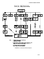
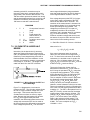
OV5. DATA RETRIEVAL OPTIONS
There are several options for data storage and
retrieval. These options are covered in detail in
Sections 2, 4, and 5. Figure OV5-1
summarizes the various possible methods.
Regardless of the method used, there are three
general approaches to retrieving data from a
datalogger.
1. On-line output of Final Storage data to a
peripheral storage device. On a regular
schedule, that storage device is brought
back to the office/lab where the data is
transferred to the computer. Another
storage device is usually taken into the field
OV-15
21X MICROLOGGER OVERVIEW
and exchanged for the one which is
retrieved so that data collection can
continue uninterrupted.
2. Bring a storage device to the datalogger
and transfer all the data that has
accumulated in Final Storage since the last
visit.
this process for IBM PC/XT/AT/PS-2's and
compatibles.
Regardless of which method is used, the
retrieval of data from the datalogger does NOT
erase those data from Final Storage. The data
remain in the ring memory until:
-
3. Retrieve the data over some form of
telecommunications link, that is, Radio
Frequency (RF), telephone, short haul
modem, multi-drop interface, or satellite.
The PC208 TELCOM program automates
-
they are written over by new data (Section
2.1)
memory is reallocated (Section 1.5)
the power to the datalogger is turned off.
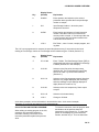
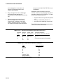
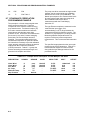
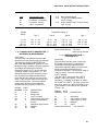
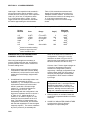
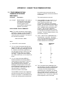
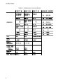
Table OV5-1 lists the instructions used with the
various methods of data retrieval.
TABLE OV5-1. Data Retrieval Methods and Related Instructions
Cassette
Tape
Storage
Module
Printer, other
Serial Device
Telecommunications
(RF, Phone, Short Haul, SC32A)
Inst. 96
*4
*8
Inst. 96,
*4
*9
*D
Inst. 96, 98
*4
*9
*D
Inst. 97
(Telecommunications Commands)
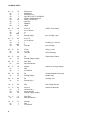
TABLE OV5-2. Data Retrieval Sections in Manual
Topic
Instr. 96
Instr. 97
*4
*8
*9
*D
Cassette Tape
Storage Module
Telecommunications
OV-16
Section in Manual
4.1, 12
12
4.1
4.2
4.2
1.8
4.3
4.4
5
21X MICROLOGGER OVERVIEW
FIGURE OV5-1. Data Retrieval Hardware Options
OV-17
21X MICROLOGGER OVERVIEW
OV6. SPECIFICATIONS
OV-18
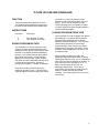
SECTION 1. FUNCTIONAL MODES
1.1 PROGRAM TABLES - *1, *2, AND *3
MODES
Data acquisition and processing functions are
controlled by instructions contained in program
tables. Programming can be separated into 2
tables, each having its own programmable
execution interval. A third table is available for
programming subroutines which may be called
by instructions in Tables 1 or 2 or by a special
interrupt. The *1 and *2 Modes are used to
access Tables 1 and 2. The *3 Mode is used to
access Subroutine Table 3.
When a program table is first entered, the
display shows the table number in the ID Field
and 00 in the Data Field. Press A and the 21X
will advance to the execution interval. If there is
an existing program in the table, enter an
instruction location number prior to A and the
21X will advance directly to the instruction (e.g.,
5 will advance to the fifth instruction in the
table).
1.1.1 EXECUTION INTERVAL
The execution interval is entered in units of
seconds as follows:
0.0125 .... 0.1 seconds, in multiples of 0.0125
0.1 .....6553 seconds, in multiples of 0.1 second
Intervals less than 0.1 second are allowed in
Table 1 only. Execution of the table is repeated
at the rate determined by this entry. The table
will not be executed if 0 is entered. Values less
than 0.1 are rounded to the nearest even
multiple of 0.0125. If the Interval is 0.1 or
greater, the 21X will not allow entry of digits
beyond 0.1.
measurement) is 256 measurements per second
(16 measurements repeated 16 times per
second).
If the specified execution interval for a table is
less than the time required to process that table,
the 21X overruns the execution interval, finishes
processing the table and waits for the next
occurrence of the execution interval before
again initiating the table (i.e., when the
execution interval is up and the table is still
executing, that execution is skipped). Since no
advantage is gained in the rate of execution with
this situation, it should be avoided by specifying
an execution interval adequate for the table
processing time.
NOTE: Whenever an overrun
occurs, decimal points are displayed
on both sides of the sixth digit of the
21X display (e.g., L O.G. in the *0
Mode).
When the Output Flag is set high, extra time is
consumed by final output processing. The
execution interval may be exceeded at this time
only, which may be acceptable. For example,
suppose it is desired to measure every 0.1
seconds and output processed data every ten
minutes. The processing time of the table is
less than 0.1 seconds except when output
occurs (every 10 minutes). With final output
processing the time required is 1 second. With
the execution interval set at 0.1 seconds, and a
one second lag between samples once every 10
minutes, 10 measurements out of 6000 (.17%)
are missed: an acceptable statistical error for
most populations.
1.1.2 SUBROUTINES
The sample rate for a 21X measurement is the
rate at which the measurement instruction can
be executed (i.e., the measurement made,
scaled with the instruction's multiplier and offset,
and the result placed in Input Storage).
Additional processing requires extra time. The
throughput rate is the rate at which a
measurement can be made and the resulting
value stored in Final Storage. The maximum
throughput rate for fast single ended
measurements (other than with the burst
Table 3 is used to enter subroutines which may
be called with Program Control Instructions in
Tables 1 and 2 or other subroutines. The group
of instructions which form a subroutine starts
with Instruction 85, Label Subroutine, and ends
with Instruction 95, End. (Section 12)
1-1
SECTION 1. FUNCTIONAL MODES
1.1.3 TABLE PRIORITY/INTERRUPTS
Table 1 execution has priority over Table 2. If
Table 2 is being executed when it is time to
execute Table 1, Table 2 will be interrupted.
After Table 1 is completed, Table 2 resumes at
the point of interruption. If the execution interval
of Table 2 coincides with Table 1, Table 1 will
be executed first, followed by Table 2.
Interrupts by Table 1 are not allowed in the
middle of a measurement or while output to
Final Storage is in process (the Output Flag, flag
0, is set high). The interrupt occurs as soon as
the measurement is completed or flag 0 is set
low.
1.1.4 COMPILING A PROGRAM
When a program is first entered, or if any
changes are made in the *1, *2, *3, *4, *A, or *C
Modes, the program must be compiled before it
starts running. The compile function checks for
programming errors and optimizes program
information for execution. If errors are detected,
the appropriate error codes are indicated on the
Display (Section 3.10). The compile function is
executed when the *0 , *6, or *B Modes are
entered and prior to saving a program listing in
the *D Mode. The compile function is only
executed after a program change has been
made; any subsequent use of any of these
Modes does not cause compiling.
When the *0, *B, or *D Mode is used to compile,
all output ports and flags are set low, the timer
(Instruction 26) is reset, and data values
contained in Input and Intermediate Storage are
RESET TO ZERO.
When the *6 Mode is used to compile data
values contained in Input Storage, the state of
flags, control ports, and the timer are
UNALTERED. Compiling always zeros
Intermediate Storage.
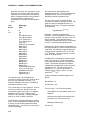
1.2 SETTING AND DISPLAYING THE
CLOCK - *5 MODE
The *5 Mode is used to display time or change
the year, day of year, or time. When *5 is
pressed, the current time is displayed. The time
parameters displayed in the *5 Mode are given
in Table 1.2-1.
1-2
The 21X powers-up with hours and minutes set
to 0 and the day and year set for the date that
the PROMs were first released by Campbell
Scientific. To set the year, day, or time, enter
the *5 Mode and advance to display the
appropriate value. Key in the desired number
and enter the value by pressing A. When a new
value for hours and minutes is entered, the
seconds are set to zero and current time is
again displayed. To exit the *5 Mode, press *.
When the time is changed, a partial recompile is
done automatically to resynchronize program
execution with real time. The resynchronization
process can change the interval of a pulse rate
measurements for one execution interval as
explained in the PULSE COUNT Instruction 3 in
Section 9.
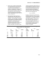
TABLE 1.2-1. Sequence of Time Parameters
in *5 Mode
Key
Display
ID:DATA
Description
*5
A
A
A
:HH:MM:SS
05:XX
05:XXXX
05:HH:MM:
Display current time
Display/enter year
Display/enter day of year
Display/enter hours:minutes
1.3 DISPLAYING AND ALTERING INPUT
MEMORY OR FLAGS - *6 MODE
The *6 Mode is used to display or change Input
Storage values and to toggle and display user
flags. If the *6 Mode is entered immediately
following any changes in program tables or the
*4 Mode, the programs will be compiled and
execution will begin.
When the *6 Mode is used to compile data
values contained in Input Storage, the state of
flags, control ports, and the timer are
UNALTERED. Compiling always zeros
Intermediate Storage.
SECTION 1. FUNCTIONAL MODES
TABLE 1.3-1. *6 Mode Commands
Key
Action
A
Advance to next location or enter
new value
Back-up to previous location
Change value in displayed
location(Key C, then value, then A)
Display/alter user flags
Display current location and allow a
location no. to be keyed in, followed
by A to jump to that location
Exit *6 Mode
B
C
D
#
*
1.3.1 DISPLAYING AND ALTERING INPUT
STORAGE
When *6 is keyed, the display will read
"06:0000". One can advance to view the value
stored in Input Storage location 1 by pressing A.
To go directly to a specific location, key in the
location number before keying A. For example,
to view the value contained in Input Storage
location 20, key in *6 20 A. The ID portion of
the display shows the last 2 digits of the location
number. If the value stored in the location being
monitored is the result of a program instruction,
the value will be updated each time the
instruction is executed.
Values may be entered into input locations using
the change command, C. While viewing the
contents of the input location in which the value
is to be entered, key C; the location number in
the ID field will disappear. Key in the desired
value and then enter it by pressing A.
If an algorithm requires parameters to be
manually modified during execution of the
program WITHOUT INTERRUPTION of the
Table execution process, the parameters can be
loaded in Input Storage locations and the *6
Mode can be used to change the values. If
values must be in place before program
execution commences, use Instruction 91 at the
beginning of the program table to prevent
execution until a flag is set high (see next
section). The initial values can be entered into
input locations using the *6 Mode after compiling
the table. The flag can then be set high to
enable the table(s).
If any program tables *1, *2, *3, or *4 output
options are altered and complied in the *0
Mode, values in Input Storage will be set to 0.
To preserve values entered in Input Storage,
compile with *6.
1.3.2 DISPLAYING AND TOGGLING USER
FLAGS
If D is keyed while the 21X is displaying a
location value, the current status of the user
flags will be displayed in the following format:
"00:01:00:10". The characters represent the
flags, the left-most digit represents Flag 1 and
right most Flag 8. A "0" indicates the flag is low
and a "1" indicates the flag is high. In the above
example, Flags 4 and 7 are set high. To toggle
a flag, simply key the corresponding number.
To return to displaying the input location, press
A.
Entering appropriate flag tests into the program
allows manual control of program execution.
For example: It is desired to be able to
manually start the execution of Table 2.
Instruction 91 is the first instruction entered in
Table 2:
01:
01:
02:
P91
25
0
If Flag
5 is set low
Go to end of program table
If Flag 5 is low, all subsequent instructions in
Table 2 will be skipped. Flag 5 can be toggled
from the *6 Mode, effectively starting and
stopping the execution of Table 2.
1.3.3 DISPLAYING AND TOGGLING PORTS
The current status of the user's ports can be
displayed by hitting "0" while looking at an input
location (e.g., *6A0). Ports are displayed left to
right as 0, 0, C6, C5, ..., C1 (exactly opposite to
the flags). A port can be toggled by pressing its
number on the keypad while in the port display
mode.
1.4 COMPILING AND LOGGING DATA *0 MODE
When the *0 Mode is entered after programming
the 21X, the program is compiled (Section 1.1.4)
and the display shows "LOG" and the numbers
of the program tables that were enabled at
1-3
SECTION 1. FUNCTIONAL MODES
compilation. The display is not updated after
entering *0.
When the *0, *B, or *D Mode is used to compile,
all output ports and flags are set low, the timer
(Instruction 26) is reset, and data values
contained in Input and Intermediate Storage are
RESET TO ZERO.
The 21X should normally be left in the *0 Mode
when logging data. This Mode requires slightly
less power than Modes which frequently update
the display.
1.5 MEMORY ALLOCATION - *A
1.5.1 INTERNAL MEMORY
There are 8 sockets on the 21X CPU board
which are used for Read Only Memory (ROM) or
Random Access Memory (RAM). The basic
21X is provided with 64K of memory: three 8K
Programmable Read Only Memory (PROM)
chips for a total of 24K ROM and five 8K RAM
chips. Appendix E describes how to change
RAM and ROM chips.
When powered-up, the 21X displays HELLO
while performing a self check; the result of the
check is then displayed. The 8 characters in the
display represent the 8 memory sockets
numbered from left to right: 1 means a good
chip is in the corresponding socket; 0 means the
socket is empty or an error was detected in the
chip. For example, when equipped with
standard memory, the display will read
"11:111111"; the five 1s on the left represent the
8K RAM chips; the three 1s on the right, the
three 8K PROMs.
There are 978 bytes allotted to program
memory. This memory may be used for 1
program table or shared among all program
tables. Tables 3.9-1 to 3.9-4 list the amount of
memory used by each program instruction.
Input Storage is used to store the results of
Input/Output and Processing Instructions. The
values stored in input locations may be
displayed using the *6 Mode (Section 1.3).
Intermediate Storage is used by Output
Processing Instructions to store the results of
intermediate calculations necessary for
averages, standard deviations, histograms, etc.
Final Storage holds output data, the results of
Output Processing Instructions which are stored
when the Output Flag is set high (Section 3.7).
The data in Final Storage can be displayed
using the *7 Mode (Section 2.3).
Figure OV2-1 illustrates the use of Input,
Intermediate, and Final Storage.
Each Input or Intermediate Storage location
requires 4 bytes of memory. Each Final Storage
location requires 2 bytes of memory. Low
resolution data points require 1 Final Storage
location and high resolution data points require
2. Section 2 describes Final Storage and data
retrieval in detail.
Table 1.5-1 lists the basic memory areas and
the amount of memory allotted to them in the
standard 21X.
TABLE 1.5-1. Memory Allocation in Standard 21X
(24K ROM, 40K RAM)
PROM
Program
Memory
System
Memory
Input
Storage*
Intermediate
Storage*
Final
Storage*]
Avail. bytes
24K
978
1022
112
256
38,592
Avail. Loc.
---
---
---
28
64
19,296
*Default allocation on power-up
1-4
SECTION 1. FUNCTIONAL MODES
1.5.2 *A MODE
The *A Mode is used to 1) determine the
number of locations allocated to Input,
Intermediate, and Final Storage; 2) repartition
this memory; 3) check the number of bytes
remaining in program memory; 4) erase Final
Storage; and 5) to completely reset the
datalogger. When *A is keyed, the first value
displayed is the number of memory locations
allocated to Input Storage. Press A to advance
through the memory values. Table 1.5-2
describes what the values seen in the *A Mode
represent.
TABLE 1.5-2. Description of *A Mode Data
Key
Entry
Display
ID: Data
*A
01: XXXX
Description of Data
The number of memory
locations currently
allocated to Input Storage.
This value can be changed
by keying in the desired
number (minimum of 28,
maximum limited by
available memory).
A
02: XXXX
The number of memory
locations currently
allocated to Intermediate
Storage. This value can
be changed by keying in
the desired number
(limited by available
memory).
A
03: XXXXX
The number of memory
locations currently
allocated to Final Storage.
This number is
automatically altered when
the number of memory
locations in Input and/or
Intermediate Storage is
changed. A minimum of
768 locations are always
retained in Final Storage.
A
04:XXXX
The number of bytes
remaining in Program
memory (978 bytes total).
Entering 978 will ERASE
ALL MEMORY and put the
21X through the initial
power-up routine.
The numbers of memory locations allocated to
Input, Intermediate and Final Storage default at
power-up to the values in Table 1.5-1.
The sizes of Input and Intermediate Storage
may be altered by keying in the desired value
and entering it by keying A. The size of Final
Storage will be adjusted automatically.
When Input Storage is increased beyond 28
locations, all of Input Storage comes out of Final
Storage and the memory previously allocated to
Input Storage (112 bytes) goes unused. This is
because memory allocated to minimum Input
Storage is bounded by write protected program
memory. When more Input Storage is required,
Input Storage must be moved to where a
contiguous block of memory is available.
One Input or Intermediate Storage location can
be exchanged for two Final Storage locations
and vice-versa. A minimum 28 Input and 768
Final Storage locations will ALWAYS be
retained. The size of Intermediate Storage may
be reduced to 0.
All data in Intermediate and Final Storage are
erased when memory is repartitioned. This
feature may be used to clear memory without
altering programming. The number of locations
does not actually need to be changed; the same
value can be keyed in and entered. After
repartitioning memory, the Tables must be
recompiled. Recompiling erases Intermediate
Storage. Recompiling with *0 erases Input
Storage; recompiling with *6 leaves Input
Storage unaltered.
If Intermediate Storage size is too small to
accommodate the programs or instructions
entered, the program will not compile and the
"E:04" ERROR CODE will be displayed; the size
of Intermediate Storage must be increased
before the program will compile. Final Storage
size can be maximized by limiting Intermediate
Storage size to the minimum number of memory
locations necessary to accommodate the
programs entered. The number of Final Storage
locations and the rate at which data are stored
determines how long it will take for Final Storage
to fill, at which point new data will write over old.
1-5
SECTION 1. FUNCTIONAL MODES
1.6 MEMORY TESTING AND SYSTEM
STATUS - *B
The *B Mode is used to 1) read the signature of
the program memory and the software PROMs,
2) display the power-up memory status, 3)
display the number of E08 occurrences (Section
3.10), 4) display the number of overrun
occurrences (Section 1.1.1), and 5) display
PROM version and revision number. Table 1.61 describes what the values seen in the *B
Mode represent. The correct signatures of the
21X PROMs are listed in Appendix B.
A signature is a number which is a function of
the data and the sequence of data in memory.
It is derived using an algorithm which assures a
99.998% probability that if either the data or its
sequence changes, the signature changes. The
signature of the program memory is used to
determine if the program tables have been
altered. During the self check on power-up, the
signature computed for a PROM is compared
with a signature stored in the PROM to
determine if a failure has occurred. The
algorithm used to calculate the signature is
described in Appendix C.
The contents of windows 8 and 9, PROM
version and version revision, are helpful in
determining what PROM is in the datalogger.
Over the years, several different PROM versions
have been released, each with operational
differences. When calling Campbell Scientific
for datalogger assistance, please have these
two numbers available.
TABLE 1.6-1. Description of *B Mode Data
Key
Entry
Display
ID: Data
*B
01: XXXXX
Program memory
Signature. The value is
dependent upon the
programming entered and
memory allotment. If the
Tables have not been
previously compiled, they
will be compiled and run.
A
02: XXXXX
First PROM Signature
03: XXXXX
Second PROM Signature
1-6
Description of Data
04: XXXXX
Third PROM Signature
A
05: XXXXX
Memory status, decimal
equivalent to the 1s and 0s
shown on power-up
(Section 1.5.1 e.g.,
11111111=255)
A
06: XXXXX
No. of E08 occurrences
(Key in 88 to reset)
A
07: XXXXX
No. of overrun occurrences
(Key in 88 to reset)
A
08: X.XXXX
PROM version number
A
09: XXXX.
Version revision number
1.7 *C MODE -- SECURITY
The *C Mode is used to secure the user's
program information. If security is activated,
then the 21X will block keyboard access to the
*1, *2, *3, *4, and *A Modes. Activated security
will also block Telecommunications access to
the *1, *2, *3, *4, *5, and *D Modes and the
Telecommunications C command. A four digit
password allows entry to the *C Mode and
becomes part of the program memory, affecting
the program signature.If security is enabled
when *C is keyed, the password must be keyed
in before one can advance to window 1. If
security is disabled, keying *C brings up window
1 immediately. In window 1 a command can be
entered to either enter a new password (1), or
temporarily disable security (00) in order to
check or alter the programming. The password
on power-up is 0000 (unless *D was used to
create a custom PROM with the password built
in), which disables security. When security is
temporarily disabled, it is possible to enter all
modes and to alter programming. Keying *0 or
*6 will automatically re-enable security, unless
the password is 0000.
Entering the 4 digit password as an indexed
value (i.e. xxxx--, entered by keying C after
entering the four digits) blocks access to the *1,
*2, *3, *4, and *A Modes, but it will allow the
user to view and change the password.
SECTION 1. FUNCTIONAL MODES
TABLE 1.7-1. *C Mode Entries and Codes
Key
Entry
Display
ID: Data
*C
12:0000
A
A
01:00
02:XXXX
A
Description
Enter current password. If
correct, then advance, else
exit *C Mode. 12:00
indicates *C Mode is not in
PROMs. If security is
disabled, *C advances
directly to window 1.
Window 1, enter command:
00 = disable security and
advance to window
2; subsequent *0 or
*6 enables security.
01 = security remains
enabled, but it
advances to
window 2 and
allows entry of a
new password.
Set new password (XXXX
is current password).
A command is entered by keying the command
number and A. When Command 1, 2, or 71 is
entered, the command number is displayed in
the ID field. The user must then key in a baud
rate code for command 1 or 2 or the command
code for the Storage Module (Table 1.8-2).
After the code is keyed in, key A to execute the
command. After a command is executed,
"13:0000" is displayed; *D must be entered
again before another command can be given.
If the 21X program has not been compiled when
a command to save the program is entered, it
will be compiled before the command is
executed.
TABLE 1.8-2. *D Mode Baud Rate and
Storage Module Codes
BAUD RATE
CODES
STORAGE MODULE
COMMAND CODES
0 - 300 baud
1 - 1200
2 - 9600
3 - 76,800
1X
Returns to window 1.
Entering 0000 disables
security (window 1 must be
set to 0).
1.8 *D MODE -- SAVE OR LOAD
PROGRAM
The *D Mode allows the user's program
information in the *1, *2, *3, *4, *A, *C (if OSX0), and *B Modes to be output to or loaded from
printer/computer (ASCII), tape, or SM192/716
Storage Module. Table execution and on-line
tape and printer outputs are suspended while in
the *D Mode. When *D is keyed, the 21X will
display "13:00".
TABLE 1.8-1. *D Mode Commands
Command
Description
1
Save ASCII Program
2
Load ASCII Program
71
Save/Load/Clear Program
from Storage Module
2X
3X
Save Program X to
Storage Module
(X=1-8)
Load Program X from
Storage Module
(X=1-8)
Erase Program X
from Storage Module
(X=1-8)
All data in Input, Intermediate and Final
Storage are erased when a command to load
a program is executed or when a program is
written to tape. If nothing is received within
30-40 seconds after giving the command to
load a program the command will be aborted
and an error code displayed (E99 for Storage
Module or ASCII). Commands 1, 2, and 71 are
the only commands that can be executed via
telecommunications (Section 5). For
commands 1 and 2, the 21X will use the baud
rate already established in telecommunications
and will be ready to receive or send the file as
soon as the command is received.
TABLE 1.8-3. Program Load Error Codes
E 98
E 99
Uncorrectable errors detected
Wrong type of file or no data received
1-7
SECTION 1. FUNCTIONAL MODES
1.8.1 TRANSFER TO COMPUTER/PRINTER
This section describes commands 1 and 2
(Table 1.8-1). TERM (PC208 Software)
automatically uses these commands for
uploading and downloading programs.
SENDING ASCII PROGRAM INFORMATION
Command 1 is to send the program listing in
ASCII. At the end of the listing, the 21X sends
control E (5 hex or decimal) twice. Except when
in telecommunications, the baud rate code must
be entered after command 1.
Table 1.8-4 is an example of the program listing
sent in response to command 1 (the actual
listing is in one column but is printed in two
columns to save space). Note that the listing
uses numbers for each mode: The numbers for
*A, *B, and *C modes are 10, 11, and 12,
respectively.
TABLE 1.8-4. Example Program Listing
From *D Command 1
MODE 2
SCAN RATE 0
MODE 3
MODE 4
1:0
2:0
MODE 10
1:28
2:64
3:19328
4:934
MODE 12
1:0
2:0
MODE 2
SCAN RATE 0
LOAD PROGRAM FROM ASCII FILE
MODE 1
SCAN RATE 2
1:P17
1:1
1:P0
Command 2 sets up the 21X to load a serial
ASCII program. The format is the same as sent
in response to command 1 (Table 1.8.4).
Except when in telecommunications, the baud
rate code must be entered after command 2.
2:P14
1:1
2:1
3:5
4:1
5:1
6:2
7:1
8:0
A download file need not follow exactly the
same format that is used when listing a program
(i.e., some of the characters sent in the listing
are not really used when a program is loaded).
Some rules which must be followed are:
3:P92
1:0
2:5
3:10
MODE 1
SCAN RATE 2
4:P71
1:2
2:1
1-8
5:P0
1. "M" must be the first character other than a
carriage return (CR) or line feed (LF). The
"M" serves the same function as "*" does
from the keyboard. The order that the
Modes are sent in does not matter (i.e., the
information for Mode 4 could be sent before
that for Mode 1).
2. "S" is necessary prior to the execution
interval (Scan rate).
3. The colons (:) are used to mark the start of
actual data.
SECTION 1. FUNCTIONAL MODES
4. A semicolon (;) tells the 21X to ignore the
rest of the line and can be used after an
entry so that a comment can be added.
There are 4 two-character control codes which
may be used to verify that the 21X receives a
file correctly:
^B ^B
(2hex, 2hex)
^C ^C
(3hex, 3hex)
^D ^D
(4hex, 4hex)
^E ^E
(5hex, 5hex)
Discard current buffer
and reset signature
Send signature for
current buffer
Load current buffer and
reset signature
Exit and compile
program
As a download file is received, the 21X buffers
the data in memory; the data is not loaded into
the editor or compiled until the 21X receives a
command to do so. The minimum file that could
be sent is the program listing, then ^E^E. ^C^C
tells the 21X to send the signature (Section C.3)
for the current buffer of data. If this signature
does not match that calculated by the sending
device, ^B^B can be sent to discard the current
buffer and reset the signature. If the signature
is correct, ^D^D can be sent to tell the 21X to
load the buffer into the editor and reset the
signature. Once the complete file has been sent
and verified, send ^E^E to compile the program
and exit the load command.
1.8.2 PROGRAM TRANSFER WITH STORAGE
MODULE
The SM192/716 Storage Module must be
connected to the 21X. Key *D, then enter
command 71. The command to save, load, or
clear a program and the program number (Table
1.8-2) is entered. After the operation is finished
"13:0000" is displayed.
The datalogger can be programmed on powerup using a Storage Module. Storage Modules
can store up to eight separate programs. If a
program is stored as program number 8, and if
the Storage Module is connected to the
datalogger serial port at power-up, program
number 8 is downloaded to the datalogger and
compiled.
1-9
SECTION 1. FUNCTIONAL MODES
This is a blank page.
1-10
SECTION 2. INTERNAL DATA STORAGE
output array. For example, the ID of 118 in
Figure 2.1-2 indicates that the 18th
instruction in Table 1 set the Output Flag
high.
2.1 FINAL STORAGE AREAS, OUTPUT
ARRAYS, AND MEMORY POINTERS
Final Storage is that portion of memory where
final, processed data are stored. Data must be
sent to Final Storage before they can be
transferred to a computer or external storage
peripheral.
The size of Final Storage is expressed in terms
of memory locations or bytes. A low resolution
data point (4 decimal characters) occupies one
memory location (2 bytes), whereas a high
resolution data point (5 decimal characters)
requires two memory locations (4 bytes). Table
1.5-1 shows the default allocation of memory
locations to Input, Intermediate, and Final
Storage. The *A Mode is used to reallocate
memory or erase Final Storage (Section 1.5). A
minimum of 768 memory locations will ALWAYS
be retained in Final Storage.
Final Storage can be represented as ring
memory (Figure 2.1-1) on which the newest data
are written over the oldest data.
FIGURE 2.1-2. Output Array ID
2) The output array ID can be set by the user
with the second parameter of Instruction 80
(Section 11). The ID can be set to any
positive integer up to 511. Instruction 80
must follow the instruction which set the
Output Flag high. This option allows the
user to make the output array ID
independent of the programming. The
program can be changed (instructions
added or deleted) without changing the
output array ID. This avoids confusion
during data reduction, especially on long
term projects where program changes or
updates are likely.
NOTE: If Instruction 80 is used to
designate Final Storage and parameter 2 is
0, the output array ID is determined by the
position of Instruction 80 or by the position
of the instruction setting the Output Flag,
whichever occurs last.
FIGURE 2.1-1. Ring Memory Representation
of Final Data Storage
Output Processing Instructions store data into
Final Storage only when the Output Flag is set
high. The string of data stored each time the
Output Flag is set high is called an output
array. The first data point in the output array is
a 4 digit Output Array ID. This ID number is set
in one of two ways:
1) In the default condition, the ID consists of
the program table number and the
Instruction Location Number of the
instruction which set the Output Flag for that
Data are stored in Final Storage before being
transmitted to an external device. There are 5
pointers which are used to keep track of data
transmission. These pointers are:
1.
2.
3.
4.
5.
Data Storage Pointer (DSP)
Display Pointer (DPTR)
Tape Pointer (TPTR)
Printer Pointer (PPTR)
Telecommunications (Modem) Pointer
(MPTR)
2-1
SECTION 2. INTERNAL DATA STORAGE
The Data Storage Pointer (DSP) is used to
determine where to store each new data point in
the Final Storage area. The DSP advances to
the next available memory location after each
new data point is stored.
The DPTR is used to recall data to the LCD
display. The positioning of this pointer and data
recall are controlled from the keyboard (*7
Mode).
The TPTR is used to control data transmission
to a cassette tape recorder. When on-line tape
transfer is activated (*4 Mode or Instruction 96,
option 00), data is transmitted to tape whenever
the DSP is a minimum of 512 memory locations
ahead of the TPTR. The TPTR may also be
positioned via the keyboard for manually
initiated data transfer to tape (*8 Mode).
The PPTR is used to control data transmission
to a printer, Storage Module, or other serial
device. Whenever on-line printer transfer is
activated (*4 Mode or Instruction 96), data
between the PPTR and DSP are transmitted.
When on-line transfer to a SM192/716 Storage
Module is activated by Instruction 96 with output
code 30, data is transmitted each time an output
array is stored in Final Storage IF THE
STORAGE MODULE IS CONNECTED TO THE
21X. If the Storage Module is not connected,
the 21X does not transmit the data nor does it
advance the PPTR to the new DSP location. It
saves the data until the Storage Module is
connected. Then, during the next execution of
Instruction 96, the 21X outputs all of the data
between the PPTR and the DSP and updates
the PPTR to the DSP location (Section 4.1)
The MPTR is used in transmitting data over a
telecommunications interface. When
Telecommunications is first entered, the MPTR
is set to the same location as the DSP.
Positioning of the MPTR is then controlled by
commands from the external calling device
(Section 5.1).
2-2
NOTE: All memory pointers are set to the
DSP location when the datalogger compiles
a program. For this reason, ALWAYS
RETRIEVE UNCOLLECTED DATA
BEFORE MAKING PROGRAM CHANGES.
For example, assume the TPTR lags the
DSP by less than 512 data points when the
datalogger program is altered. On
compiling, the TPTR is positioned with the
DSP, losing reference to the data that was
intended to be transferred to tape. The
data is not automatically transferred and
appears as a discontinuity in the data file.
Until the ring memory wraps around and
data overwrite occurs, the data may be
recovered using the *8 Mode. This
scenario is also true for the PPTR and data
intended for a Storage Module.
2.2 DATA OUTPUT FORMAT AND
RANGE LIMITS
Data are stored internally in Campbell
Scientific's Final Storage Format (Appendix
C.2). Data may be sent to Final Storage in
either LOW RESOLUTION or HIGH
RESOLUTION format. Low resolution is the
default. To change the resolution, Instruction 78
(Section 11) must precede the Output
Instructions in the program table.
2.2.1 RESOLUTION AND RANGE LIMITS
Low resolution data is a 2 byte format with 3 or 4
significant digits and a maximum magnitude of
±6999. High resolution data is a 4 byte format
with 5 significant digits and a maximum possible
output value of ±99999 (see Table 2.2-1 below).
TABLE 2.2-1. Resolution Range Limits of
21X Data
Minimum
Magnitude
Resolution
Zero
Low
High
0.000 ±0.001
0.0000 ±.00001
Maximum
Magnitude
±6999.
±99999.
SECTION 2. INTERNAL DATA STORAGE
The resolution of the low resolution format is
reduced to 3 significant digits when the first (left
most) digit is 7 or greater (Table 2.2-2). Thus, it
may be necessary to use high resolution output
or an offset to maintain the desired resolution of
a measurement. For example, if water level is
to be measured and output to the nearest 0.01
foot, the level must be less than 70 feet for low
resolution output to display the 0.01 foot
increment. If the water level is expected to
range from 50 to 80 feet the data could either be
output in high resolution or could be offset by 20
feet. (transforming the range to 30 to 60 feet.).
TABLE 2.2-2. Decimal Location in Low
Resolution Format
Absolute Value
0
7
70
700
6.999
69.99
- 699.9
- 6999.
Decimal Location
0.0000305. A description of Campbell
Scientific's floating point format may be found in
the description of the J and K
telecommunications commands in Appendix C.
2.3 DISPLAYING STORED DATA ON
KEYBOARD/DISPLAY - *7 MODE
The *7 Mode is used to display Final Storage
data. Enter the Mode by keying *7. The display
will show "07:XXXXX", where XXXXX is the
Final Storage location (DSP) where the next
data will be stored. Two options are available:
1.
Press A to advance and display the
output array ID of the oldest array in
Final Storage.
2.
Enter a Final Storage location number.
When A is pressed, the DPTR will jump
to the location entered and, if it is not at
the start of an array, advance to the first
start of array. The display will show the
Array ID.
X.XXX
XX.XX
XXX.X
XXXX.
While output data have the limits described
above, the computations performed in the 21X
are done in floating point arithmetic. Values are
rounded when converting to Final Storage
Format.
2.2.2 INPUT AND INTERMEDIATE STORAGE
DATA FORMAT
In Input and Intermediate Storage, numbers are
stored and processed in a binary format with a
23 bit binary mantissa and a 6 bit binary
exponent. The largest and smallest numbers
that can be stored and processed are 9 x 1018
and 1 x 10-19, respectively. The size of the
number determines the resolution of the
arithmetic. A rough approximation of the
resolution is that it is better than 1 in the seventh
digit. For example, the resolution of 97,386,924
is better than 10. The resolution of
0.0086731924 is better than 0.000000001.
A precise calculation of the resolution of a
number may be determined by representing the
number as a mantissa between .5 and 1
multiplied by 2 raised to some integer power.
The resolution is the product of that power of 2
and 2-24. For example, representing 478 as
.9336 * 29, the resolution is 29 * 2-24 = 2-15 =
Repeated use of the A key advances through
the output array, while use of the B key backs
the DPTR through memory.
The Final Storage location of the data point
being viewed may be displayed by keying #. At
this point, another location may be entered,
followed by A to jump to the start of the output
array equal to or just ahead of the location
entered. Whenever a location number is
displayed by keying #, the corresponding data
point can be displayed by keying C. To advance
to the start of the next output array, key #A. To
back up one output array key #B.
TABLE 2.3-1. *7 Mode Command Summary
Key
Action
A
B
#
Advance to next data point
Back-up to previous data point
Display location number of currently
displayed data point value
Display value of current location
Advance to start of next output array
Back-up to previous output array
C
#A
#B
2-3
SECTION 2. INTERNAL DATA STORAGE
This is a blank page.
2-4
SECTION 3. INSTRUCTION SET BASICS
The instructions used to program the 21X are divided into 4 types: Input/Output (I/O), Processing,
Output Processing, and Program Control. I/O Instructions are used to make measurements and
store the readings in input locations or to initiate analog or digital port output. Processing
Instructions perform numerical operations using data from Input Storage locations and place the
results back into specified Input Storage locations. Output Processing Instructions provide a
method for generating time or event dependent data summaries from processed sensor readings
residing in specified Input Storage locations. Program Control Instructions are used to direct
program execution based on time and/or conditional tests on input data and to direct output to
external devices.
Instructions are identified by a number. Each instruction has a number of parameters which give
the 21X the information it needs to execute the instruction.
The set of instructions available in the 21X is determined by the Programmable Read Only
Memory chips (PROMS) that are installed. Appendix B lists the software options available.
3.1 PARAMETER DATA TYPES
There are 3 different data types used for
Instruction parameters: Floating Point (FP), 4
digit integers (4), and 2 digit integers (2). In the
listings of the instruction parameters (Sections
9-12), the parameter data type is identified by its
abbreviation. Different data types are used to
allow the 21X to make the most efficient use of
its memory.
Floating Point parameters are used to enter
numeric constants for calibrations or arithmetic
operations. While it is only possible to enter 5
digits (magnitude ±.00001 to ±99999.), the
internal format has a much greater range
(1x10-19 to 9x1018, Section 2.2.1).
3.2 REPETITIONS
The repetitions parameter on many of the I/O,
Processing, and Output Processing Instructions
is used to repeat the instruction on a number of
sequential Input Channels or Input Storage
locations. For example, if you have 4 differential
voltage measurements to make on the same
voltage range, wire the inputs to sequential
channels and instead of entering the Differential
Voltage Measurement Instruction 4 times, enter
it once with 4 repetitions. The instruction will
make 4 measurements starting on the specified
channel number and continuing through the 3
succeeding differential channels, with the results
being stored in the specified input location and
the 3 succeeding input locations. Averages for
all 4 measurements can be calculated by
entering the Average Instruction with 4
repetitions.
When several of the same type of
measurements are to be made but the
calibrations of the sensors are different, it
requires less time to use a single measurement
instruction with repetitions and then apply the
calibrations with Instruction 53 than it does to
enter the instruction several times in order to
use different multipliers and offsets. This is due
to the set up and calibration time for each
measurement instruction. However, if time is
not a constraint, separate instructions may make
the program easier to follow.
3.3 ENTERING NEGATIVE NUMBERS
After keying in a number, press C or "-" to
change the number's sign. On floating point
numbers a minus sign (-) will appear to the left
of the number.
Excitation voltages in millivolts for I/O
Instructions are 4 digit integers; when C is
pressed, minus signs (-) will appear to the right
of the number indicating a negative excitation.
Even though this display is the same as that
indicating an indexed input location, (Section
3.4) there is no indexing effect on excitation
voltage.
3.4 INDEXING INPUT LOCATIONS
When used within a Loop, the parameters for
input locations can be Indexed to the loop
3-1
SECTION 3. INSTRUCTION SET BASICS
counter. The loop counter is added to the
indexed value to determine the actual input
location the instruction acts on. Normally the
loop counter is incremented by 1 after each
pass through the loop. Instruction 90, Step
Loop Index, allows the increment step to be
changed. See Instructions 87 and 90, Section
12, for more details.
the sensor being measured. Using the smallest
possible range will result in the best resolution
for the measurement.
Two different integration sequences are
possible. The slow integration, 16.67
milliseconds, is one 60 Hz cycle and rejects
noise from 60 Hz AC line power as well as
having better rejection of random noise than the
fast integration. A PROM with 50Hz rejection is
available for countries whose electric utilities
operate at 50Hz (Appendix B).
To index an input location (4 digit integer) key C
after keying the value but before entering the
parameter. Two minus signs (-) will be
displayed to the right of the parameter.
When a voltage input exceeds the range
programmed, the value stored is the maximum
negative number, displayed in the *6 Mode as
-99999. In output data from Final Storage this
becomes -6999 in low resolution or -99999. in
high resolution.
3.5 VOLTAGE RANGE AND
OVERRANGE DETECTION
The RANGE code parameter on Input/Output
Instructions is used to specify the full scale
voltage range of the measurement and the
integration period for the measurement (Table
3.5-1).
An input voltage greater than +8 volts on one of
the analog inputs will result in errors and
possible overranging on the other analog inputs.
Voltages greater than 16 volts may permanently
damage the 21X.
Select the smallest full scale range that is
greater than or equal to the full scale output of
TABLE 3.5-1. Input Voltage Ranges and Codes
Range Code
Slow
Fast
16.67ms
250µs
Integ.
Integ.
1
11
2
12
3
13
4
14
5
15
Full Scale Range
±5
±15
±50
±500
±5000
millivolts
millivolts
millivolts
millivolts
millivolts
Resolution*
0.33
1.
3.33
33.3
333.
microvolts
microvolts
microvolts
microvolts
microvolts
*Differential measurement, resolution for single-ended measurement is twice value shown.
3.6 OUTPUT PROCESSING
Most Output Processing Instructions require
both an intermediate processing operation and a
final processing operation. For example, when
the Average Instruction, 71, is executed, the
intermediate processing operation increments a
sample count and adds each new Input Storage
value to a cumulative total residing in
Intermediate Storage. When the Output Flag is
set, the final processing operation divides the
total by the number of sample counts, stores the
resulting average in Final Storage and zeros the
3-2
value in Intermediate Storage so that the
process starts over with the next execution.
Final Storage is the default destination of data
output by Output Processing Instructions
(Sections OV1.2, 1.5, 2.1). Instruction 80 may
be used to direct output to Input Storage or to
Final Storage.
Output Processing Instructions requiring
intermediate processing sample the specified
input location(s) each time the Output Instruction
is executed, NOT necessarily each time the
SECTION 3. INSTRUCTION SET BASICS
location value is updated by an I/O Instruction.
For example: Suppose a temperature
measurement is initiated by Table 1 which has
an execution interval of 1 second. The
instructions to output the average temperature
every 10 minutes are in Table 2 which has an
execution interval of 10 seconds. The
temperature will be measured 600 times in the
10 minute period, but the average will be the
result of only 60 of those measurements
because the instruction to average is executed
only one tenth as often as the instruction to
make the measurement.
Final processing occurs only when the Output
Flag is set (Section 3.7.1). The Output Flag,
Flag 0, is set at desired intervals or in response
to specified conditions by using an appropriate
Program Control Instruction (Section 11).
3.7 USE OF FLAGS: OUTPUT AND
PROGRAM CONTROL
There are 10 flags which may be used in 21X
programs. Two of the flags have functions with
Output Processing Instructions: Flag 0 controls
final processing and data storage, and Flag 9
can disable intermediate processing. Flags 1-8
may be used as desired in programming the
21X. Flags 0 and 9 are automatically set low at
the beginning of the program table. Flags 1-8
remain unchanged until acted on by a Program
Control Instruction or until manually toggled from
the *6 Mode.
TABLE 3.7-1. Flag Description
Flag 0
Flag 1 to 8 Flag 9
-
Output Flag
User Flags
Intermediate Processing
Disable Flag
Flags are set with Program Control Instructions.
The Output Flag, Flag 0, and the intermediate
processing disable flag, Flag 9, will always be
set low if the set high condition is not met. The
status of flags 1-8 are not changed if a
conditional test is false.
3.7.1 THE OUTPUT FLAG
A set of processed data values is placed in
Final Storage by Output Processing Instructions
when the Output Flag, Flag 0, is set high. This
set of
data is called an output array. The Output Flag
is set according to time or event dependent
intervals using Program Control Instructions
specified by the user. The Output Flag is set
low at the beginning of each table.
Each group of Output Processing Instructions
creating an output array must be preceded by a
Program Control Instruction that sets the Output
Flag.
Output is most often desired at fixed intervals;
this is accomplished with Instruction 92, If Time,
which checks the clock to see if it is X minutes
into a Y minute interval. If the time condition is
met, a command is executed. Output at the
beginning of the interval by making Parameter 1,
time into the interval, 0. Parameter 2, the time
interval in minutes, is how often output will
occur; i.e., the Output Interval. Enter 10 for
parameter 3, the command code, to set Flag 0
high. Instruction 92 is followed in the program
table by the Output Instructions which define the
output array desired.
The time interval is synchronized to 24 hour
time; output will occur on each integer multiple
of the Output Interval starting from midnight (0
minutes). If the Output Interval is not an even
divisor of 1440 minutes (24 hours), the last
output interval of the day will be less than the
specified time interval. Output will occur at
midnight and will resume synchronized to the
new day.
NOTE: If the Output Flag is already
set high and the test condition of a
subsequent Program Control
Instruction acting on the flag fails,
the flag is set low. This feature
eliminates having to enter another
instruction to specifically reset the
Output Flag at the end of an output
array before proceeding to another
group of Output Instructions with a
different output interval (see example
in OV4.3).
3.7.2 THE INTERMEDIATE PROCESSING
DISABLE FLAG
The Intermediate Processing Disable Flag, Flag
9, suspends intermediate processing when it is
3-3
SECTION 3. INSTRUCTION SET BASICS
set high. This flag is used to restrict sampling
for averages, totals, maxima, minima, etc., to
times when certain criteria are met. The flag is
automatically set low at the beginning of the
program table.
As an example, suppose it is desired to obtain a
wind speed rose incorporating only wind speeds
greater than or equal to 4.5 m/s. The wind
speed rose is computed using the Histogram
Instruction 75, and wind speed is stored in Input
location 14, in m/s. Instruction 89 is placed just
before Instruction 75 and is used to set Flag 9
high if the wind speed is less than 4.5 m/s:
TABLE 3.7-2. Example of the Use of Flag 9
Inst. Param.
Loc.
No.
X
X+1
X+2
Entry
Description
P
1
2
3
89
14
4
4.5
4
P
P
1
19
75
86
29
If wind speed < 4.5 m/s
Wind speed location
Comparison: <
Minimum wind speed
for histogram
Set Flag 9 high
Histogram
Do
Set Flag 9 Low
NOTE: Flag 9 is automatically reset
the same as Flag 0. If the
intermediate processing disable flag
is already set high and the test
condition of a subsequent Program
Control Instruction acting on Flag 9
fails, the flag is set low. This feature
eliminates having to enter another
instruction to specifically reset Flag 9
before proceeding to another group
of test conditions.
3.8 PROGRAM CONTROL LOGICAL
CONSTRUCTIONS
Most of the Program Control Instructions have a
command code parameter which is used to
specify the action to be taken if the condition
tested in the instruction is true. Table 3.8-1 lists
these codes.
TABLE 3.8-1. Command Codes
0
1-9, 77-99
10-19
20-29
30
31
32
41-46
51-56
61-66
71-76
-
Go to end of program table
Call Subroutine 1-9, 77-99
Set Flag 0-9 high
Set Flag 0-9 low
Then Do
Exit loop if true
Exit loop if false
Set port 1 - 6 high
Set port 1 - 6 low
Toggle port 1 - 6
Pulse port 1 - 6 100 ms
3.8.1 IF THEN/ELSE COMPARISONS
When Command 30, THEN DO, is used with
one of the IF Instructions, 88-92, the instruction
is followed immediately by instructions to
execute if the comparison is true. The Else
Instruction, 94, is optional and is followed by the
instructions to execute if the comparison is
false. The End Instruction, 95, marks the end
of the branching started by the IF Instruction.
Subsequent instructions are executed
regardless of the outcome of the comparison
(Figure 3.8-1).
3.7.3 USER FLAGS
Flags 1-8 are not dedicated to a specific
purpose and are available to the user for
general programming needs. The user flags
can be manually toggled from the keyboard in
the *6 Mode (Section 1.3) or from a computer
using TERM's monitor feature. By inserting flag
tests (Instruction 91) at appropriate points in the
program, the user can manually set flags to
direct program execution.
3-4
FIGURE 3.8-1. If Then/Else Execution
Sequence
SECTION 3. INSTRUCTION SET BASICS
If Then/Else comparisons may be nested to form
logical AND or OR branching. Figure 3.8-2
illustrates an AND construction. If conditions A
and B are true, the instructions included between
IF B and the first End Instruction will be
executed. If either of the conditions is false,
execution will jump to the corresponding End
Instruction, skipping the instructions between.
encountered, execution branches to the END
Instruction 95 which closes the case test (see
Instruction 93).
3.8.2 END, INSTRUCTION 95
END, Instruction 95, is required to mark the end
of:
1. A Subroutine (starts with Instruction 87)
2. A Loop (starts with Instruction 85)
3. An IF ... THEN DO sequence (starts with
one of Instructions 89-93 with the THEN DO
command 30).
4. A case statement (starts with Instruction 93)
The IF instructions 89-93 require Instruction 95
only when the THEN DO command 30 is used.
If one of the above instructions is used without
the corresponding END, the 21X will display
error 22 when compiling the program. Error 21
is displayed if END is used without being
preceded by one of these instructions (Section
3.10).
FIGURE 3.8-2. Logical AND Construction
Figure 3.8-3 illustrates the instruction sequence
that will result in subroutine X being executed if
either A or B is true.
IF A (88-92 with command 30)
Call subroutine X (86, command=X)
ELSE (94)
IF B (88-92 with command 30)
Call subroutine X (86, command=X)
END B (95)
END A (95)
FIGURE 3.8-3. Logical OR Construction
A logical OR can also be constructed by setting
a flag if a comparison is true. (The flag is
cleared before making the comparisons.) After
all comparisons have been made, execute the
desired instructions if the flag is set.
The Begin Case Instruction 93 and If Case
Instruction 83 allow a series of tests on the value
in an input location. The case test is started with
Instruction 93 which specifies the location to test.
A series of Instructions 83 are then used to
compare the value in the location with fixed
values. When the value in the input location is
less than the fixed value specified in Instruction
83 the command in that Instruction 83 is
executed; when the next Instruction 83 is
An END instruction is always paired with the
most recent instruction that requires an END and
does not already have one. A way of visualizing
this is to draw lines between each instruction
requiring an END and the END paired with it (as
in Figure 3.8-2). The lines must not cross. To
debug logic or find a missing or extra END error,
list the program and draw the lines.
Subroutines can be called from other
subroutines; they cannot be embedded within
other subroutines. A subroutine must end before
another subroutine begins (Error 20). Any loops
or IF...THEN DO sequences started within a
subroutine must end before the subroutine.
3.8.3 NESTING
A branching or loop instruction which occurs
before a previous branch or loop has been
closed with the END instruction is nested. The
maximum nesting level is 9 deep. Error 30 is
displayed when attempting to compile a program
which is nested too deep.
The Loop Instruction, 87, counts as 1 level.
Instructions 86, 88, 89, 91, and 92 each count as
one level when used with the THEN DO
command 30. Use of Else, Instruction 94, also
counts as one nesting level each time it is used.
For example, the AND construction above is
3-5
SECTION 3. INSTRUCTION SET BASICS
nested 2 deep while the OR construction is
nested 3 deep. Branching and loop nesting
starts at zero within each subroutine and then
returns to the previous level after returning from
the subroutine.
Subroutine calls do not count as nesting with
the above instructions. They have a separate
nesting limit of seven (Instruction 85, Section
12).
Any number of groups of nested instructions
may be used in any of the three Programming
Tables. The number of groups is only restricted
by the program memory available.
3.9 INSTRUCTION MEMORY AND
EXECUTION TIME
The standard 21X has 978 bytes of program
memory available for the programs entered in
the *1, *2, and *3 program tables. Each
instruction also makes use of varying numbers of
Input, Intermediate, and Final Storage locations.
The following tables list the memory used by
each instruction and the approximate time
required to execute the instruction.
TABLE 3.9-1. Input/Output Instruction Memory
R = No. of Reps.
D = Delay
INSTRUCTION
1
2
3
4
5
6
7
8
9
10
11
12
13
14
16
17
18
19
20
21
22
23
26
101
102
103
104
INPUT
LOC.
VOLT (SE)
R
VOLT (DIFF)
R
PULSE
R
EX-DEL-SE
R
AC HALF BR
R
FULL BR
R
3W HALF BR
R
EX-DEL-DIFF R
FULL BR-MEX R
BATT. VOLT
1
TEMP (107)
R
RH (207)
R
TEMP-TC SE
R
TEMP-TC DIF R
TEMP-RTD
R
TEMP-INTERNL 1
TIME
1
SIGNATURE
1
PORT SET
1
ANALOG OUT 1
EXCIT-DEL
1
BURST MODE R
TIMER
1 or 0
SDM-INT8
25
SDM-SW8
16
SDM-AO4
0
SDM-CD16
6
MEMORY
EXECUTION TIME (ms)
PROG.
MEASUREMENT RANGE
BYTES
1-4 or NA
5.*
15
38.0 + 19.2R
8.4 + 3.7R
15
36.9 + 38.0R
7.8 + 6.9R
15
0.2 + 1.2R
20
38.0 + (19.2 + D)R
8.1 + (4.4 + D)R
18
38.8 + 40R
10.7 + 7.5R
18
41.8 + 73.0R
10.5 + 13.1R
18
41.2 + 76.8R
10.6 + 16.2R
20
38.1 + (19.2 + D)2R
8.1 + (4.2 + D)2R
19
76.7 + 149.6R
15.7 + 28.2R
4
7.6
15
5.0 + 8.4R
17
7.9 + 7.0R
18
40.8 + 23.2R
18
39.2 + 42.7R
15
0.4 + 2.7R
4
14.0
7
1.4
4
1200
4
0.3
5
10.5
11
1.0 + D
4
11-14
5.5 + 2.4R
5.5 + 3.7R
5.3 + (2.8 + D)R
7.5 + 5.1R
7.6 + 7.4R
7.1 + 11.0R
5.3 + (2.8 + D)2R
9.9 + 16.7R
7.9 + 6.7R
7.8 + 8.5R
0.54 to reset, 0.25 to load into location
6
* Range 5 uses a 1.67ms integration time; the other "slow integration" ranges (1-4) use 16.67ms
integrations. Range 15 uses a 25µs integration (ranges 11 - 14 use 250µs). The execution times for
instructions using range 15 are faster than those given for ranges 11 - 14 by approximately 225µs per rep
for single-ended measurements, and 450µs per rep for differential.
3-6
SECTION 3. INSTRUCTION SET BASICS
TABLE 3.9-2. Processing Instruction Memory and Execution Times
R = No. of Reps.
INSTRUCTION
30
31
32
33
34
35
36
37
38
39
40
41
42
43
44
45
46
47
48
49
50
51
53
54
55
56
57
58
59
60
61
Z=F
Z=X
Z=Z+1
Z=X+Y
Z=X+F
Z=X-Y
Z=X*Y
Z=X*F
Z=X/Y
Z=SQRT(X)
Z=LN(X)
Z=EXP(X)
Z=1/X
Z=ABS(X)
Z=FRAC(X)
Z=INT(X)
Z=X MOD F
Z=XY
Z=SIN(X)
SPA MAX
SPA MIN
SPA AVG
A*X+B
BLOCK MOVE
POLYNOMIAL
SAT VP
WDT-VP
LP FILTER
X/(1-X)
FFT
INDIR MOVE
62
66
COV/COR
ARC TAN
INPUT
LOC.
MEMORY
INTER.
PROG.
LOC.
BYTES
EXECUTION TIME (ms)
1
0
8
0.3
1
0
6
0.5
1
0
4
0.6
1
0
8
1.1
1
0
10
0.9
1
0
8
1.1
1
0
8
1.2
1
0
10
0.9
1
0
8
2.7
1
0
6
12.0
1
0
6
7.4
1
0
6
5.9
1
0
6
2.6
1
0
6
0.7
1
0
6
0.3
1
0
6
1.0
1
0
10
3.2
1
0
8
13.3
1
0
6
6.5
1 or 2
0
7
1.5 + 0.9 (swath-1)
1 or 2
0
7
1.7 + 0.9 (swath-1)
1
0
7
3.3 + 0.6 (swath-1)
4
0
36
2.5 + 0.4 scaling pair
R
0
10
0.18 + 0.17R
R
0
31
1.2 + R(2.0 + 0.4 * order)
1
0
6
4.2
1
0
10
8.1
R
R
13
0.5 + 2.2R
1
0
9
0.4 + 3.0R
See Instruction Description Section 10
1
0
6
0.35 neither indexed
0.54 one location indexed
0.73 both locations indexed
See Instruction Description Section 10
1
0
8
6.7
3-7
SECTION 3. INSTRUCTION SET BASICS
TABLE 3.9-3. Output Instruction Memory and Execution Times
R = No. of Reps.
INSTRUCTION
INTER.
LOC.
69 WIND VECTOR
MEMORY
FINAL
VALUES1
70 SAMPLE
71 AVERAGE
72 TOTALIZE
73 MAXIMIZE
74 MINIMIZE
75 HISTOGRAM
0
1+R
R
(1 or 2)R
(1 or 2)R
1+bins*R
(2, 3, or 4)R 12
Options 00, 01, 02
Options 10, 11, 12
R
5
R
7
R
7
(1,2,or3)R 8
(1,2,or3)R 8
bins*R
24
77 REAL TIME
78 RESOLUTION
79 SMPL ON MM
80 STORE AREA
81 RAINFLOW
HISTOGRAM
82 STD. DEV.
0
0
R
0
1 to 4
0
R
0
1Output
2+9R
PROG.
BYTES
4
3
7
5
EXECUTION TIME (ms)
FLAG 0 LOW
FLAG 0 HIGH
3.5 + 17.5R
3.5 + 16R
0.1
0.9+ 0.5R
0.6+ 0.5R
0.9+ 1.7R
0.9+ 1.7R
0.4+ 3.1R
0.1
0.4
0.3
3.5 + 75R
3.5 + 30R
0.4+ 0.6R
2.1+ 3.0R
1.1+ 1.0R
1.3+ 2.8R
1.3+ 2.8R
0.9+
R(3.3+2.8*bins)
1.0
0.4
1.1
See Instruction Description Section 11
1+2R
R
7
values may be sent to either Final Storage or Input Storage with Instruction 80.
TABLE 3.9-4. Program Control Instruction Memory and Execution Times
INSTRUCTION
INTER.
LOC.
83 IF CASE <F
85 LABEL SUBR
86 DO
87 LOOP
88 IF X<=>Y
89 IF X<=>F
90 LOOP INDEX
91 IF FLAG
92 IF TIME
93 BEGIN CASE
94 ELSE
95 END
96 SERIAL OUT
97 INIT.TELE.
98 SEND CHAR.
3-8
0
0
0
1
0
0
0
0
1
1
0
0
0
7
0
MEMORY
PROG.
BYTES
9
3
5
9
10
12
3
6
11
8
4
4
3
23
4
EXECUTION TIME (ms)
0.5
0.0
0.1
0.2
0.6
0.4
0.5
0.2
0.3
0.2
0.2
0.2
SECTION 3. INSTRUCTION SET BASICS
3.10 ERROR CODES
There are four types of errors flagged by the
21X: Compile, Run Time, Editor, and *D Mode.
When an error is detected an E is displayed
followed by the 2 digit error code.
Compile errors are errors in programming
which are detected once the program is keyed in
and compiled for the first time (*0, *6, or *B
Mode entered).
Run Time errors are detected while the
program is running. Error 31 is the result of a
programming error. Error 8 is the result of a
hardware and software "watchdog" that checks
the processor state, software timers, and
program related counters. The watchdog will
attempt to reset the processor and program
execution if it finds that the processor has
bombed or is neglecting standard system
updates, or if the counters are out of allowable
limits. Error code 08 is flagged when the
watchdog performs this reset.
Error 8 is occasionally caused by voltage surges
or transients. Frequent repetitions of E08 are
indicative of a hardware problem or a software
bug and should be reported to Campbell
Scientific. The 21X keeps track of the number of
times (up to 99) that E08 has occurred. The
number can be displayed and reset with the
Telecommunications A command (Section 5.1).
Editor errors are detected as soon as an
incorrect value is entered and are displayed
immediately.
*D Mode errors indicate problems with saving or
loading a program. Only the error code is
displayed.
TABLE 3.10-1. Error Codes
Code
03
04
08
09
11
20
21
22
24
25
26
30
31
40
40
60
61
97
98
99
Type
Editor
Compile
Run Time
Run Time
Editor
Compile
Compile
Compile
Compile
Compile
Compile
Compile
Run Time
Compile
Editor
Compile
Compile
*D MODE
*D MODE
*D MODE
Description
Program table full
Intermediate Storage full
21X reset by watchdog timer
Data sent to unallocated Input Storage
Attempt to allocate more Input or Intermediate Storage than is available
SUBROUTINE encountered before END of previous subroutine
END without IF, LOOP or SUBROUTINE
Missing END, nonexistent SUBROUTINE
ELSE in SUBROUTINE without IF
ELSE without IF
EXIT LOOP without LOOP
IF and/or LOOP nested too deep
SUBROUTINES nested too deep
Table 2 Execution interval too short
Instruction not in PROM
Inadequate Input Storage for FFT
Burst Mode Scan Rate too short
Tape data not received within 30 seconds
Uncorrectable errors detected
Wrong file type, editor error or program not received
3-9
SECTION 3. INSTRUCTION SET BASICS
This is a blank page.
3-10
SECTION 4. EXTERNAL STORAGE PERIPHERALS
External data storage devices are used to provide a data transfer medium that the user can carry from
the test site to the lab and to supplement the internal storage capacity of the 21X, allowing longer
periods between visits to the site. The standard data storage peripherals for the 21X are the cassette
tape (Section 4.3) and the Storage Module (Section 4.4). Output to a printer or related device is also
possible (Section 4.5). These peripherals are connected to the 21X through the 9 pin serial connector.
Data output to a peripheral device can take place ON-LINE (automatically, as part of the 21X's routine
operation) or it can be MANUALLY INITIATED. On-line data transfer is accomplished with Instruction 96
or with the *4 Mode (Section 4.1). Manual initiation is done in the *8 or *9 Modes (Section 4.2).
Regardless of the method, the source of any data transferred is Final Storage.
A modem is another type of peripheral that can be connected to the 21X. Communication via a modem
(Telecommunications) is discussed in Section 5.
The 21X can output data to multiple peripherals (i.e., a tape recorder, modem, and Storage Module
could all be connected at the same time). However, only one cassette recorder and only one modem
may be connected to the 21X at any one time. It is possible to connect two Storage Modules, although it
is seldom necessary.
The 21X can tell whether or not a SM192 or SM716 Storage Module is present. When Instruction 96 or
*9 is used to send data to one of these Storage Modules, the 21X will not send data if the Storage
Module is not connected (Section 4.4.2).
4.1 ON-LINE DATA TRANSFER INSTRUCTION 96, *4 MODE
On-line data transfer is accomplished with
Instruction 96 entered in the datalogger
program. The *4 Mode is retained from earlier
software to maintain compatibility with existing
programs. Use only one method to enable
output. If using Instruction 96, do not enable
output in the *4 Mode.
4.1.1 INSTRUCTION 96
Instruction 96 enables output to external storage
peripherals under program control. This
instruction must be included in the datalogger
program for on-line data transfer to take place.
Instruction 96 needs to be included only once in
the program tables, and should follow the Output
Processing Instructions. The suggested
programming sequence is:
1. Set the Output Flag.
2. If you wish to set the output array ID, enter
Instruction 80 (Section 11).
3. Enter the appropriate Output Processing
Instructions.
4. Enter Instruction 96 to enable the on-line
transfer of Final Storage data to the
specified device. If outputting to both tape
and a Storage Module or printer option,
Instruction 96 must be entered twice.
Instruction 96 has a single parameter which
specifies the peripheral to enable. Table 4.1-1
lists the output device codes.
TABLE 4.1-1. Output Device Codes for
Instruction 96
CODE
00
1x
2x
30
31
DEVICE
Tape. Data transferred in blocks
of 512 Final Storage Locations
Printer, Printable ASCII
Printer, Binary
SM192/716 Storage Module
Send filemark to SM192/716
x = BAUD RATE CODE
0
300
1
1200
2
9600
3
76,800
4-1
SECTION 4. EXTERNAL STORAGE PERIPHERALS
Only one of the options 1x, 2x, or 30 may be
used in a program. If using a SM64 Storage
Module, output code 21 should be used. Use of
the SM192/716 is discussed further in Section
4.4, print output formats are discussed in
Section 4.5.
Section 4.3 contains specifics on the cassette
recorder. Note that tape operation is for above
freezing temperatures only.
4.1.2 *4 MODE
The *4 Mode may be used in place of Instruction
96 to enable or disable printer and/or cassette
tape output and to set the printer baud rate. The
first parameter is a two digit number determining
the tape and printer status. The second is the
baud rate code. To enter a different status, key
in the appropriate code from Table 4.1-2,
followed by "A". Printer data is sent in the
printable ASCII format only (Section 4.5). If
tape or printer status is changed during
execution of the program tables, execution stops
until the programs are recompiled. Instruction
96 should be used to send data to the
SM192/716 Storage Modules. Do not use *4 if
Instruction 96 is used in the program.
TABLE 4.1-2. *4 Mode Parameters and
Codes
Key
Display
ID:DATA
*4
A
04:00
01:XX
A
02:XX
Description
Output Enable Code
(e.g., "10" means tape
enabled, printer disabled)
Baud Rate Code
Output Enable Codes
Code
Description
X0
printer disabled
X1
printer enabled, ASCII
0X
tape disabled
1X
tape enabled
Baud Rate Codes
Code
Baud Rate
00
300
01
1200
02
9600
03
76,800
4-2
4.2 MANUALLY INITIATED DATA
OUTPUT - *8 AND *9 MODES
Data may be transferred to tape using the *8
Mode and to printer or Storage Module using the
*9 Mode. These Modes allow the user to
retrieve a specific block of data, on demand,
regardless of whether or not the 21X is
programmed for on-line data output.
If external storage peripherals (cassette,
Storage Module, etc.) are not left on-line, the
maximum allowable time between visiting the
site to retrieve data must be calculated to insure
that data placed in Final Storage are not written
over before they are collected. In order to make
this calculation, users must determine: (1) the
size of Final Storage, (2) the number of output
arrays being generated, (3) the number of low
and/or high resolution data points included in
each output array, and (4) the rate at which
output arrays are stored in Final Storage. When
calculating the number of data points per output
array, remember to add 1 overhead data point
(2 bytes) per array for the output array ID.
For example, assume that 19,296 locations are
assigned to Final Storage (*A Mode), and that 1
output array, containing the Array ID (1 memory
location), 9 low resolution data points (9 memory
locations) and 5 high resolution data points (10
memory locations) is stored each hour. In
addition, an output array with the Array ID and 5
high resolution data points (11 memory
locations) is stored daily. This is a total of 491
memory locations per day ((20 x 24) + 11).
19,296 divided by 491 = 39.3 days. Therefore,
the 21X would have to be visited every 39 days
to retrieve data, because write-over would begin
in the 40th day.
4.2.1 MANUAL TAPE DUMP *8 MODE
If on-line tape storage is enabled, entering the *8
Mode will suspend it. If left in the *8 Mode, online storage will be re-enabled if no key entries
are made for 3.4 minutes. Setting up the tape
recorder is discussed in Section 4.3.4.
SECTION 4. EXTERNAL STORAGE PERIPHERALS
a field site, dump the residual data before
removing the tape.
TABLE 4.2-1. *8 Mode Entries
Key
Display
ID:DATA
*8
08:00
Enter *8 Mode, key A to
advance to first window.
A
01:XXXXX
Start of Dump location,
initially the TPTR location, a
different location may be
keyed in if desired.
A
02:XXXXX
End of Dump location,
initially the DSP location,
a different location may
be keyed in if desired.
A
03:00
Description
Ready to Dump, to initiate
dump, key any number
then A. While dumping,
"08:" will be displayed in
the ID field and the
location number in the
Data field. The location
number will stop
incrementing when the
dump is complete.
If the TPTR is at the same location as the DSP,
then a block of 512 "dummy" values are
transferred. This provides a means of checking
the 21X/cassette connections and the cassette
operation. During data playback, the PC201
and C20 Cassette Interfaces recognize dummy
values and do not transmit them.
When on-line tape transfer is not enabled and
the *8 Mode is used to dump new data, the start
of dump pointer (TPTR) will remain where it was
when the dump was completed or aborted until
the next time the *8 Mode is entered. If the End
of Dump location (window 2) is changed while in
the *8 Mode, the TPTR will be set to its previous
value when the *8 Mode is exited. Changing the
program and compiling moves the TPTR to the
current DSP location.
When on-line, the 21X dumps data to tape in
blocks of 512 Final Storage locations. Residual
data is data which has accumulated since the
last full block. When picking up a data tape from
To dump the residual data enter the *8 Mode,
advance directly to window 3 and initiate a
dump. Because data are written to tape in fixed
blocks of 512 locations, the TPTR may be in the
middle of an output array. Entering a location
for the TPTR, even the location originally
displayed, will result in the TPTR being moved to
the first output array start marker following the
location entered. Thus, the portion of the array
following the original TPTR location would not be
written to tape.
To use the *8 Mode to transfer all data from
Final Storage to tape, enter a start of dump
location number which is 1 greater than the end
of dump location, advance to ready to dump
(03:) and key any number and A. Data transfer
occurs immediately and is completed when the
display shows "08:" and the current DSP
location.
To dump a portion of the data in Final Storage,
key in the start and end locations before
initiating the dump. The locations can be
determined by viewing the contents of Final
Storage in the *7 Mode. By saving the current
location of the DSP and using it for the starting
location on the next visit to the site, only the
data stored between visits are transferred to
tape.
NOTE: A tape dump can be aborted by
keying #. However, since it cannot be
aborted in the middle of a 512 data point
block, up to 5 seconds may elapse before
the tape stops.
4.2.2 MANUAL STORAGE MODULE OR PRINTER
DUMP - *9 MODE
Using the *9 Mode, data in Final Storage can be
transmitted as ASCII or binary data out the
serial port by manually initiating a dump. If online printing is enabled with Instruction 96 or the
*4 Mode, entering *9 will stop it. On-line printing
will be re-enabled if no keyboard entries are
made for 3.4 minutes. Return to the *0 Mode
when the dump is completed.
4-3
SECTION 4. EXTERNAL STORAGE PERIPHERALS
When on-line Storage Module or printer transfer
is not enabled and the *9 Mode is used to dump
new data, the start of dump pointer (PPTR) will
remain where it was when the dump was
completed or aborted until the next time the *9
Mode is entered. If the End of Dump location
(window 2) is changed while in the *9 Mode, the
TPTR will be set to its previous value when the
*9 Mode is exited. Changing the program and
compiling moves the PPTR to the current DSP
location.
NOTE: A printer dump is aborted by
keying #.
TABLE 4.2-2. *9 Mode Entries
Key
Display
ID:DATA
*9
09:00
Description
Output Code
1X Printable ASCII
2X Final Storage Format
30 SM192/716 Storage
Module
31 Send filemark to
SM192/716
x = Baud Rate Code
0
300
1
1200
2
9600
3
76800
A
A
A
4-4
01:XXXXX
02:XXXXX
03:00
Start of Dump location,
initially the PPTR location,
a different location may be
keyed in if desired. To
dump all data in Final
Storage, enter into window
#1 a number 1 greater
than the End of Dump
location.
End of Dump location,
initially the DSP location, a
different location may be
keyed in if desired.
Ready to Dump, to
initiate dump, key any
number then A. While
dumping, "09:" will be
displayed in the ID field
and the location
number in the Data
field. The location
number will stop
incrementing when the
dump is complete.
4.3 CASSETTE TAPE OPTION
The Model RC35 Cassette Tape Recorder or
equivalent can be left attached to the 21X for
continuous on-line data recording or it can be
periodically taken to the 21X site for the
manually initiated retrieval of the data
accumulated in Final Storage. The *8 Mode is
used to manually initiate tape transfer.
4.3.1 CASSETTE RECORDER
The RC35 Cassette Recorder offered by
Campbell Scientific is an inexpensive recorder
for use with the 21X (also compatible with the
CR10 and CR7 dataloggers). The
record/playback function of each RC35 is tested
by Campbell Scientific along with a head
alignment procedure prior to shipment.
21X/RC35 connections are made with the
SC92A Cassette Write Only Interface or the
SC93A Cassette Read/Write Interface. The 21X
turns the RC35 on and off by switching power
through the DC power input.
TABLE 4.3-1 Cassette Recorder
Specifications
Power
6VDC (provided by 21X
through SC92A or SC93A); 4
AA size batteries;
120VAC/6VDC adapter
Current Drain
while Recording
200mA typ./5 sec.,
300 max.
Tape Length
C-60 recommended
Tape Quality
Normal bias, high quality
(e.g., TDK, Maxell)
External Inputs
Mic., DC In, Monitor, and
Remote
Operating
Temperature
0° to +40°C
SECTION 4. EXTERNAL STORAGE PERIPHERALS
POWER SUPPLY
The 21X's internal power supply will power the
recorder during periods of data transfer, but will
NOT be available to play, advance, or back-up
tapes. In order to perform these functions
during setup and check-out operations, the
recorder requires 4 alkaline AA batteries or the
120 VAC adapter.
OPERATING TEMPERATURE LIMITATIONS
The cassette recorder is recommended for use
in an environmental operating temperature
range of 0° to +40°C. Temperatures below 0°C
may cause tape speed variation in excess of
that which can be tolerated during playback.
Data Recorded with the RC35 outside the 0°C
to 40°C range may be unreadable.
VOLUME CONTROL
When recording data, the RC35's volume setting
does not matter. The recorder is equipped with
an automatic gain control which controls the
recorded signal level. For playback, a mid range
volume setting is normally required.
interface is only necessary if the 21X has
special software for transferring programs via
tape (Appendix B).
The SC92A and SC93A have a combination
backshell circuit card and 9-pin connector which
attaches to the serial I/O connector on the 21X.
The SC92A has two plugs which connect to the
POWER and MIC jacks on the recorder. The
SC93A has three plugs which connect to the
POWER, MIC and EAR (or MONITOR) jacks on
the recorder. Both cables transform 12V from
the 21X to 6V to power the recorder during
periods of data transfer. Additional circuitry
shapes the data signal waveform.
4.3.3 TAPE FORMAT
Data tapes generated by the 21X are read by
the PC201 tape read card for the IBM PC/XT/AT
or by the C20 Cassette Interface. The C20
decodes the tape and transmits the data in
ASCII via a standard RS232 interface.
TABLE 4.3-2. Format 2 Specifications
CASSETTE TAPES
Data
Binary
Normal bias, high quality cassette tapes are
recommended for use with the recorder. The
more expensive high bias chromium oxide tapes
will NOT perform satisfactorily. Although the
use of C-90 tapes is generally successful,
Campbell Scientific recommends the use of C60 (30 minutes per side) cassettes. TDK,
Maxell, and equivalent quality cassette tapes
perform well and are readily available. Bargainpriced tapes have often performed poorly and
are not recommended.
Low Resolution
2 bytes/data point
High Resolution
4 bytes/data point
C-60 Capacity
(Lo Res.)
180,000 data points
(1 side only)
Data Transfer
Rate (Lo Res.)
100 data points/sec.
Block Size
locations
512 Final Storage
New tapes are often tightly wound, creating
enough drag or pressure to cause the tape
recorder to "pop" out of the record mode. This
potential loss of data may be overcome by fastforward/rewinding the entire tape before placing
it in service.
4.3.2 CASSETTE CONNECTOR INTERFACE
CABLES
A Cassette Interface Cable is required to
connect the cassette recorder to the 21X. Two
models are available. The SC92A is a WRITE
ONLY interface. The SC93A READ/WRITE
4.3.4 CONNECTING TAPE RECORDER TO 21X
The procedure for setting up the 21X and
cassette recorder for transfer to tape is as
follows:
1. Load a cassette in the recorder and
advance the tape forward until the tape
leader is past the recording head. (Internal
batteries or AC power required.)
2. Connect the SC92A or SC93A to the 9-pin
serial I/O port.
4-5
SECTION 4. EXTERNAL STORAGE PERIPHERALS
3. Insert the plugs on the free end of the
SC92A or SC93A into the DC-IN and MIC
(and Ear if SC93A) jacks on the recorder.
old. The Storage Modules must be retrieved
before the module configured as ring memory
wraps around memory a second time.
4. Simultaneously press the RECORD and
PLAY buttons on the recorder to set it for
recording. With the DC-IN Jack plugged in,
the tape will not move until the dump occurs.
4.4.2 STORAGE MODULE USE WITH
INSTRUCTION 96
5. To test connections manually initiate
transfer by keying in the *8 commands as
listed in Table 4.2-1. The tape should
advance as data is transferred. If the Start
of dump location is equal to the End of
dump location, the 21X will write a "dummy"
block of data to tape.
If you are leaving the recorder on-line (tape
enabled with Instruction 96) it is a good idea to
write a dummy block of data to tape (5 above) to
ensure that the recorder is correctly connected.
Leave the 21X in the *0 Mode.
4.4 STORAGE MODULE (SM192/716)
The Storage Module stores data in battery
backed RAM. Backup is provided by an internal
lithium battery. Operating power is supplied by
the 21X over pin 1 of the 9 pin connector. When
power is applied to the Storage Module, a File
Mark is placed in the data (if a File Mark is not
the last data point already in storage).
The File Mark separates data. For example, if
you retrieve data from one 21X, disconnect the
Storage Module and connect it to a second 21X,
a File Mark is placed in the data. This mark
follows the data from the first 21X but precedes
the data from the second.
The SM192 has 192K bytes of RAM storage; the
SM716 has 716K bytes. Both can be configured
as either ring or fill and stop memory.
4.4.1 USE OF TWO STORAGE MODULES
It is possible to connect two Storage Modules to
the 21X for on-line storage. One module must
be configured as fill and stop and the other as
ring memory (see Storage Module operator's
manual for configuring information). Data is
written to both modules simultaneously. The
module configured as fill and stop quits
accepting data once it is full while that with the
ring memory continues to store new data over
4-6
When output to the Storage Module is enabled
with Instruction 96, the Storage Module(s) may
be either left with the 21X for on-line data
transfer and periodically exchanged, or brought
to the site for data transfer.
USE OF STORAGE MODULE TO PICK UP
DATA
The 21X can tell when the Storage Module is
connected. Each time Instruction 96 is executed
and there is data to output, the 21X checks for
the presence of the Storage Module. If a
Storage Module is not connected no data are
sent and the Printer Pointer (PPTR, Section 2.1)
is not advanced.
When a Storage Module is connected, two
things happen:
1. Immediately upon connection, a File Mark is
placed in the Storage Module Memory
following the last data stored.
2. During the next execution of Instruction 96,
the 21X detects the Storage Module and
outputs all data between the PPTR and the
DSP location.
The File Mark allows the operator to distinguish
blocks of data from different dataloggers or from
different visits to the field.
If the SM is just brought to the site to pick-up
data, the SC90 Serial Line Monitor can be used
to visually confirm that data were transferred.
The SC90 contains an LED which lights during
data transmission. When the light goes OFF
data transfer is complete and the SM can be
disconnected from the 21X.
4.4.3 *9 DUMP TO STORAGE MODULE
In addition to the on-line data output procedures
described above, output from 21X Final Storage
to the SM192 and SM716 can be manually
initiated in the *9 Mode. The procedure for
setting up and transferring data is as follows:
SECTION 4. EXTERNAL STORAGE PERIPHERALS
1. Connect the Storage Module to the 21X
using the SC12 cable.
2. Enter the appropriate commands as listed
in Table 4.2-2.
4.5 PRINTER OUTPUT FORMATS
Printer output can be sent in the binary Final
Storage Format (Appendix C.2) or Printable
ASCII. If using the *4 Mode to enable on-line
output, Printable ASCII is the only format
available.
In the Printable ASCII format each data point is
preceded by a 2 digit data point ID and a + or sign. The ID and fixed spacing of the data
points make particular points easy to find on a
printed output. This format requires 10 bytes
per data point to store on disk.
Figure 4.5-1 shows both high and low resolution
data points in a 12 data point output array. The
example data contains Day, Hour-Minute, and
Seconds in the 2nd - 4th data points. The
output array ID and time values (year, day, hourminute, and seconds) are always 4 character
numbers, even when high resolution output is
specified.
Each full line of data contains 8 data points (79
characters including spaces), plus a carriage
return (CR) and line feed (LF). If the last data
point in a full line is high resolution, it is followed
immediately with a CR and LF. If it is low
resolution, the line is terminated with a space,
CR and LF. Lines of data containing less than 8
data points are terminated similarly after the last
data point.
FIGURE 4.5-1. Example of 21X Printable ASCII Output Format
4-7
SECTION 4. EXTERNAL STORAGE PERIPHERALS
This is a blank page.
4-8
SECTION 5. TELECOMMUNICATIONS
Telecommunications allows a computer to retrieve data directly from Final Storage and may be
used to program the 21X and monitor sensor readings in real time. Any user communication with
the 21X that makes use of a computer or terminal instead of the 21X keyboard is through
Telecommunications.
Telecommunications can take place over a variety of links including:
•
•
•
•
•
telephone
radio frequency
short haul modem
SC32A and ribbon cable
multi-drop interface and coax cable
This section does not cover the technical interface details for any of these links. Those details
are covered in Section 6 and in the individual manuals for the devices.
Data retrieval can take place in either ASCII or BINARY. The BINARY format is five times more
compact than ASCII. The shorter transmission times for binary result in lower long distance
telephone charges and more reliable data transfer. On "noisy" links shorter blocks of data are
more likely to get through without interruption.
In addition to more efficient data transfer, binary data retrieval makes use of a signature for error
detection. The signature algorithm assures a 99.998% probability that if either the data or its
sequence changes, the signature changes.
The PC208 Datalogger Support Software for PCs and compatibles contains the program
TELCOM which automates data retrieval and TERM which will upload and download programs
and monitor Input Storage. The PC208 package has been designed to meet the most common
needs in datalogger support and telecommunications. This section in not intended to furnish
sufficient detail to write Telecommunications software. Appendix C contains some details of
binary data transfer and Campbell Scientific's binary data format.
This section emphasizes the commands that a person would use when manually (i.e., entered by
hand) interrogating or programming the 21X via a computer/terminal. These commands and the
responses to them are sent in the American Standard Code for Information Interchange (ASCII).
The Remote Keyboard State (Section 5.2) allows the user with a computer/terminal to use the
same commands as the 21X keyboard.
5.1 TELECOMMUNICATIONS
COMMANDS
When the 21X is rung by a modem, it answers
(enables the modem) almost immediately.
Several carriage returns (CR) must be sent from
the computer to allow the 21X to set its baud
rate to that of the modem/terminal (300, 1200,
9600, or 76,800). Once the baud rate is set, the
21X sends the prompt, *, signaling that it is
ready to receive a command.
GENERAL RULES governing the
telecommunications commands are:
1. * from datalogger means "ready for
command".
2. All commands are of the form: [no.]letter,
where the number may or may not be
optional.
3. Valid characters are the numbers 0-9, the
capital letters A-L, the colon (:), and the
carriage return (CR).
4. An illegal character increments a counter
and zeros the command buffer, returning *.
5-1
SECTION 5. TELECOMMUNICATIONS
5. CR to datalogger means "execute".
6. CRLF from datalogger means "executing
command".
7. ANY character besides a CR sent to the
datalogger with a legal command in its
buffer causes the datalogger to abort the
command sequence with CRLF* and to zero
the command buffer.
8. All commands return a response code,
usually at least a checksum.
9. The checksum includes all characters sent
by the datalogger since the last *, including
the echoed command sequence, excluding
only the checksum itself. The checksum is
formed by summing the ASCII values,
without parity, of the transmitted characters.
The largest possible checksum value is
8191. Each time 8191 is exceeded, the 21X
starts the count over; e.g., if the sum of the
ASCII values is 8192, the checksum is 0.
10. Commands that return Campbell Scientific
binary format data (F and K commands)
return a signature (Appendix C).
The 21X sends ASCII data with 8 data bits, no
parity, plus one start bit and one stop bit.
After answering a ring, or completing a
command, the 21X waits about 40 seconds (147
seconds in the Remote Keyboard State) for a
valid character to arrive. If a valid character is
not received, the 21X "hangs up". Some
modems are quite noisy when not on line; it is
possible for valid characters to appear in the
noise pattern. To insure that this situation does
not keep the 21X in telecommunications, the
21X counts all the invalid characters it receives
from the time it answers a ring, and terminates
communication after receiving 150 invalid
characters.
The 21X continues to execute its measurement
and processing tasks while servicing the
telecommunication requests. If the processing
overhead is large (short execution interval), the
processing tasks will slow the
telecommunication functions. In a worst case
situation, the 21X interrupts the processing
tasks to transmit a data point every 0.1 second.
The best way to become familiar with the
Telecommunication Commands is to try them
from a terminal connected to the 21X via the
SC32A or other modem interface (Section 6.5).
Telecommunications Commands are described
in the following Table. The Data Storage Pointer
(DSP) and Telecommunications Modem Pointer
(MPTR) referred to in the table are described in
Section 2.1.
TABLE 5.1-1. Telecommunications Commands
Command
A
Description
STATUS - Datalogger returns Reference, the DSP location; the number of
filled Final Storage locations; Version of datalogger; Errors #1 and #2 where
#1 is the number of E08 and #2 is the number of overrun that have occurred
(cleared by entering 8888A); Memory status, the decimal number (in ASCII
characters) that is the equivalent of the 8 bit binary number shown as the
result of the memory check on power-up; Location of MPTR; and Checksum.
All in the following format:
R+xxxxx F+xxxxx Vx Exx xx Mxxxx L+xxxxx Cxxxx
If data are stored while in telecommunications, the A command must be
issued to update the Reference to the new DSP.
[no. of arrays]B
5-2
BACK-UP - MPTR is backed-up the specified number of output arrays (no
number defaults to 1) and advanced to the nearest start of array. 21X sends
the MPTR Location and Checksum: L+xxxxx Cxxxx
SECTION 5. TELECOMMUNICATIONS
[YR:DAY:HR:MM:SS]C
RESET/SEND TIME - If time is entered the time is reset. If only 2 colons are
in the time string, HR:MM:SS is assumed; 3 colons means DAY:HR:MM:SS.
If only the C is entered, time is unaltered. 21X returns year, Julian day,
hr:min:sec, and Checksum: Y:xx Dxxxx Txx:xx:xx Cxxxx
[no. of arrays]D
ASCII DUMP - If necessary, the MPTR is advanced to the next start of array.
21X sends the number of arrays specified (no number defaults to 1) or the
number of arrays between MPTR and Reference, whichever is smaller,
CRLF, Location, Checksum.
E
[no. of loc.]F
[F.S. loc. no.]G
2718H
[loc. no.]I
3142J
K
[Password]L
End call. Datalogger sends CRLF only.
BINARY DUMP - Used in TELCOM (PC208). See Appendix C.
MOVE MPTR - MPTR is moved to specified Final Storage location. The
location number must be entered. 21X sends Location and Checksum:
L+xxxxx Cxxxx
REMOTE KEYBOARD - 21X sends the prompt ">" and is ready to execute
standard keyboard commands (Section 5.2).
Display/change value at Input Storage location. 21X sends the value stored
at the location. A new value and CR may then be sent. 21X sends
checksum. If no new value is sent (CR only) the location value will remain the
same.
TOGGLE FLAGS AND SET UP FOR K COMMAND - Used in the Monitor
Mode and with the Heads Up Display. See Appendix C for details.
CURRENT INFORMATION - In response to the K command, the 21X sends
datalogger time, user flag status, the data at the input locations requested in
the J command, and Final Storage Data if requested by the J command.
Used in the Monitor Mode and with Heads Up Display. See Appendix C.
Unlocks security (See *C Mode, Section 1.7). 21X sends ON or OFF and
checksum: OFF Cxxxx
5.2 REMOTE PROGRAMMING OF THE
21X
The 21X can be programmed via
telecommunications using the PC208 software
or manually through the Remote Keyboard
State.
The PC208 Datalogger Support Software was
developed for use with IBM or compatible PC's.
Datalogger programs are developed on the
computer using the program editor EDLOG and
downloaded to the datalogger with the terminal
emulator program TERM.
The 21X is placed in the Remote Keyboard
State by sending "2718H" and a carriage return
(CR). The 21X responds by sending a CR, line
feed (LF), and the prompt ">". The 21X is then
ready to receive the standard keyboard
commands (Section OV3); it recognizes all the
standard 21X keyboard characters plus the
decimal point. While in the Remote Keyboard
State, the 21X sends the ASCII character
control Q (17 decimal) after each user entry.
Entering *0 returns the 21X to the
telecommunications command state.
It is important to remember that the Remote
Keyboard State is still within
Telecommunications. Entering *0 exits the
Remote Keyboard and returns the datalogger to
the Telecommunications Command State,
5-3
SECTION 5. TELECOMMUNICATIONS
awaiting another command. So the user can
step back and forth between the
Telecommunications Command State and the
Remote Keyboard State.
Remote Keyboard State, use *6 (Section 1.1.4).
The 21X display will show "LOG" when *0 is
executed via telecommunications. It will not
indicate active tables (enter *0 via the keyboard
and the display will show the tables).
Keying *0 will compile and run the 21X program
if program changes have been made. To
compile and run the program without leaving the
2718H
Telecommunications
Command
State
5-4
*0
Remote
Keyboard
State
SECTION 6. 9 PIN SERIAL INPUT/OUTPUT
6.1 PIN DESCRIPTION
All external communication peripherals connect
to the 21X through the 9-pin serial I/O connector
(Figure 6.1-1). Table 6.1-1 gives a brief
description of each pin's function.
FIGURE 6.1-1. 9 Pin Connector
TABLE 6.1-1. Pin Description
ABR
PIN
O
I
PIN
ABR
I/O
1
5V
O
2
G
=
=
=
=
Abbreviation for the function name.
Pin number.
Signal Out of the 21X to a peripheral.
Signal Into the 21X from a peripheral.
Description
PIN
5V: Sources 5V DC, used
to power peripherals.
Ground: Provides a power
return for pin 1 (5V), and is
used as a reference for
voltage levels.
3
RING
I
Ring: When raised by a
peripheral the 21X enters
telecommunications.
4
RXD
I
Receive Data: Serial data
transmitted by a peripheral
are received on pin 4.
5
ME
O
Modem Enable: Raised by
the 21X after the ring line has
been raised.
ABR
I/O
Description
6
PE
O
7
G
I/O Ground, common with pin
2.
8
TE
O
Tape Enable: Powers the
cassette recorder during
data transfer to tape.
9
TXD
O
Transmit Data: Serial data
are transmitted from the
21X to peripherals on pin 9;
logic low marking (0V) logic
high spacing (5V) standard
asynchronous ASCII, 8
data bits, no parity, 1 start
bit, 1 stop bit, 300, 1200,
9600, 76,800 baud (user
selectable).
Printer Enable: Raised to
enable Storage Module or
other print device.
6-1
SECTION 6. 9 PIN SERIAL INPUT/OUTPUT
6.2 ENABLING PERIPHERALS
Several peripherals may be connected in parallel
to the 9-pin port. The 21X directs data to a
particular peripheral by raising the voltage on a
specific pin dedicated to the peripheral; the
peripheral is enabled when the pin goes high.
Three pins are dedicated to specific devices,
Tape Enable pin 8, Modem Enable pin 5, and
Print Enable pin 6.
Tape Enable (TE), pin 8, is raised to 12 volts to
power the tape recorder. The SC92A or SC93A
Cassette Interface regulates the 12 volts to 6
volts to power the RC35 recorder. Only one
tape interface and recorder may be connected
to the 21X.
Modem Enable (ME), pin 5, is raised to enable
a modem that has raised the ring line. Only one
modem/terminal may be connected to the 21X.
Print Enable (PE), pin 6, is raised to enable a
Storage Module or other print peripheral. Print
peripherals are defined as peripherals which
have an asynchronous serial communications
port used to RECEIVE data transferred by the
21X. In most cases the peripheral is a printer,
but could also be an on-line computer or other
device. It is possible to have more than one
print peripheral connected to the 21X at one
time, as long as they don't load down the TXD
line (e.g., two Storage Modules, Section 4.4.1);
all connected receive the same data.
6.3 INTERRUPTING DATA TRANSFER
TO STORAGE PERIPHERALS
Instruction 96 is used for on-line data transfer to
peripherals (Section 4.1). Data transfer is
aborted when a modem raises the Ring line and
the 21X then enters Telecommunications
(Section 5, 6.4). After the 21X exits
Telecommunications, data transfer to the
peripheral is resumed the next time Instruction
96 is executed, or, if activated by the *4 Mode,
at the completion of the next active table.
The *8 and *9 Modes are used to position the
Memory Pointers, and to manually initiate data
transfer from Final Storage to a peripheral. If
the # key is pressed during data transfer, the
transfer is stopped and the display shows the
Final Storage location where the pointer
stopped.
6-2
Data transfer can be stopped as follows:
1. Printable ASCII - after every output array.
2. Binary - after every Final Storage location.
3. Tape - after every block (512 Final Storage
locations).
6.4 TELECOMMUNICATIONS - MODEM
PERIPHERALS
Any serial communication device which raises
the Ring line and holds it high until the ME line is
raised is a modem. The DC112 phone modem,
RF95 RF modem, MD9 Multi-Drop Interface,
and the SC32A RS232 interface used with
computers or terminals are modems.
When a modem raises the Ring line, the 21X
responds by raising the ME line. The 21X must
be sent carriage returns until it sets the baud
rate. When the baud rate is set, the 21X sends
a carriage return, line feed, *.
The ME line is held high until the 21X receives
an E to exit telecommunications. The ME is
also lowered if a character is not received after
40 seconds in the Telecommunications
Command State or 147 seconds in the Remote
Keyboard State. The colon in 21X display is not
shown while the 21X is in telecommunications.
Some modems are quite noisy when not on line;
it is possible for valid characters to appear in the
noise pattern. For this reason, the 21X counts
all the invalid characters it receives from the
time it answers a ring and terminates
communication (lowers the ME line and returns
to the *0 Mode) after receiving 150 invalid
characters.
6.5 INTERFACING WITH COMPUTERS,
TERMINALS, AND PRINTERS
This section deals with some of the basics of
serial communication between the 21X and
common computer equipment. If you have an
IBM compatible PC, the PC208 Datalogger
Support Software takes care of the software
protocol required in communicating with the
21X. This section does not discuss modem
interfaces other than the SC32A. Please refer
to the PC208 and modem operator's manuals
for interfacing details on other modems.
SECTION 6. 9 PIN SERIAL INPUT/OUTPUT
6.5.1 SC32A INTERFACE
Most computers, terminals, and printers require
the SC32A Optically Isolated RS232 Interface
for a "direct" connection to the 21X. The SC32A
raises the 21X's ring line when it receives
characters from the computer or terminal, and
converts the 21X's logic levels (0V logic low, 5V
logic high) to RS232 logic levels.
The SC32A 25 pin port is configured as Data
Communications Equipment (DCE) which allows
direct connection to Data Terminal Equipment
(DTE), which includes most PCs and printers.
For connection to DCE devices such as
modems and some computers, a null modem
cable is required.
When the SC32A receives a character from the
computer or terminal (pin 2), 5V is applied to the
datalogger Ring line (pin 3) for one second or
until the Modem Enable line (ME) goes high.
The 21X waits approximately 40 seconds to
receive carriage returns, which it uses to
establish baud rate. After the baud rate is set
the 21X transmits a carriage return, line feed, *,
and enters the Telecommunications Command
State (Section 5). If the carriage returns are not
received within the 40 seconds, the 21X "hangs
up".
NOTE: The SC32A has a jumper. With the
jumper in place the SC32A blocks printer
data and passes data only when the 21X is
in Telecommunications.
Table 6.5-1 lists the most common RS232
configuration for Data Terminal Equipment.
TABLE 6.5-1. DTE Pin Configuration
PIN = 25-pin connector number
ABR = Abbreviation for the function name
O = Signal Out of the terminal to another
device
I = Signal Into the terminal from another device
PIN
ABR
I/O
2
TD
O
Transmitted Data: Data is
transmitted from the terminal
on this line.
3
RD
I
Received Data: Data is
received by the terminal on
this line.
4
RTS
O
Request to Send: The
terminal raises this line to ask
a receiving device if the
terminal can transmit data.
5
CTS
I
Clear to Send: The receiving
device raises this line to let
the terminal know that the
receiving device is ready to
accept data.
20
DTR
O
Data Terminal Ready: The
terminal raises this line to tell
the modem to connect itself
to the telephone line.
6
DSR
I
Data Set Ready: The
modem raises this line to tell
the terminal that the modem
is connected to the phone
line.
8
DCD
I
Data Carrier Detect: The
modem raises this line to
tell the terminal that the
modem is receiving a valid
carrier signal from the
phone line.
22
RI
I
Ring Indicator: The modem
raises this line to tell the
terminal that the phone is
ringing.
7
SG
6.5.2 COMPUTER/TERMINAL REQUIREMENTS
Computers, terminals and printers are usually
configured as Data Terminal Equipment (DTE).
Pins 4 and 20 are used as handshake lines,
which are set high when the serial port is
enabled. Power for the SC32A is taken from
these pins. For equipment configured as DTE a
direct ribbon cable connects the modem/terminal
to the SC32A. Clear to Send (CTS) pin 5, Data
Set Ready (DSR) pin 6, and Received Line
Signal Detect (RLSD) pin 8 are held high by the
SC32A (when the RS232 section is powered)
which should satisfy hardware handshake
requirements of the modem/terminal.
FUNCTION
Signal Ground: Voltages are
measured relative to this
point.
6-3
SECTION 6. 9 PIN SERIAL INPUT/OUTPUT
If the computer is configured as DCE equipment
(pin 2 is an input for RD), a null modem cable is
required. See the SC32A manual for details.
6.5.3 COMMUNICATION PROTOCOL/TROUBLE
SHOOTING
The ASCII standard defines an alphabet
consisting of 128 different characters where
each character corresponds to a number, letter,
symbol, or control code.
An ASCII character is a binary digital code
composed of a combination of seven "bits",
each bit having a binary state of 1 or more. For
example, the binary equivalent for the ASCII
character "1" is 0110001 (decimal 49).
ASCII characters are transmitted one bit at a
time, starting with the first (least significant) bit.
During data transmission the marking condition
is used to denote the binary state 1, and the
spacing condition for the binary state 0. The
signal is considered marking when the voltage is
more negative than minus three volts with
respect to ground, and spacing when the voltage
is more positive than plus three volts.
Most computers use 8-bits (1 byte) for data
communications. The eighth bit is sometimes
used for a type of error checking called paritychecking. Even parity binary numbers have an
even number of 1's, odd-parity characters have
an odd number of 1's. When parity checking is
used, the eighth bit is set to either a 1 or a 0 to
make the parity of the character correct. The
21X ignores the eighth bit of a character that is
receives, and transmits the eighth bit as a binary
0. This method is generally described as "no
parity".
To separate ASCII characters a Start bit is sent
before the first data bit, and a Stop bit is sent
after the eighth data bit. The start bit is always
a space, and the stop bit is always a mark.
Between characters the signal is in the marking
condition.
Figure 6.5-1 shows how the ASCII character "1"
is transmitted. The SC32A interface transmits
spacing and marking voltages which are positive
and negative, as shown. Signal voltages at the
21X I/O port are 5 volts in the spacing condition,
and 0 volts in the marking condition.
FIGURE 6.5-1. Transmitting the ASCII Character 1
BAUD RATE
DUPLEX
BAUD RATE is the number of bits transmitted
per second. The 21X can communicate at 300,
1200, 9600, and 76,800 baud. In the
Telecommunications State, the 21X will set its
baud rate to match the baud rate of the modem.
Full duplex means that two devices can
communicate in both directions simultaneously.
Half duplex means that the two devices must
send and receive alternately. Full duplex should
always be specified when communicating with
Campbell Scientific peripherals and modems.
However, communication between some
Campbell Scientific modems (such as the RF95
RF modem) is carried out in a half duplex
fashion. This can affect the way commands
should be sent to and received from such a
The baud rate of the modem or computer is
usually set with dip switches or programmed
from the keyboard. The instrument's instruction
manual should explain how to set it.
6-4
SECTION 6. 9 PIN SERIAL INPUT/OUTPUT
modem, especially when implemented by
computer software.
To overcome the limitations of half duplex, some
communications links expect a terminal sending
data to also write the data to the screen. This
saves the remote device having to echo that
data back. If, when communicating with a
Campbell Scientific device, characters are
displayed twice (in pairs), it is likely that the
terminal is set to half duplex rather than the
correct setting of full duplex.
IF NOTHING HAPPENS
If the 21X is connected via the SC32A interface
to a terminal or computer and * is not received
after sending carriage returns:
1. Verify that the 21X has power and that the
cables connecting the devices are securely
connected.
2. Verify that the port of the computer or
terminal is an asynchronous serial
communications port configured as DTE
(see Table 6.5-2). The most common
problems occur when the user tries to use a
parallel port, or doesn't know the port
address (i.e. COM1 or COM2). IBM, and
most compatibles come with a Diagnostic
disk which can be used to identify ports,
and their addresses. If the serial port is
standard equipment, then the operators
manual should give you this information.
Some serial ports such as the Super Serial
Card for Apple computers, can be
configured as DTE or DCE with a jumper
block. Pin functions must match with Table
6.5-1.
If you are using a computer, then a program or
communication software must be used to enable
the serial port, and to make the computer
function as a terminal. The port should be
enabled for 300, 1200, or 9600 baud, 8 data
bits, 1 stop bit, and no parity. TERM (PC208
Software) provides this function for IBM
PC/XT/AT/PS-2's and compatibles.
If you are not sure that your computer or
terminal is sending or receiving characters,
there is a simple way to verify it. Set the duplex to
full. Next, take a paper clip and connect one
end to pin 2, and the other end to pin 3 of the
serial port. Each character typed on the
keyboard will be displayed only if transmitted
from the terminal on pin 2, and received on pin 3
(with half duplex the character will be displayed
once if it is not transmitted, or twice if it is
transmitted).
IF GARBAGE APPEARS
If garbage characters appear on the
modem/terminal, check that the
modem/terminal's baud rate is supported by the
21X. If the baud rate is correct, verify that the
modem/terminal is set for 8 Data bits, and no
Parity. Garbage will appear if 7 Data bits and no
Parity are used. If the modem/terminal is set to
8 Data bits and even or odd Parity,
communication cannot be established.
6-5
SECTION 6. 9 PIN SERIAL INPUT/OUTPUT
This is a blank page.
6-6
SECTION 7. MEASUREMENT PROGRAMMING EXAMPLES
This section gives some examples of Input Programming for common sensors used with the 21X. These
examples detail only the connections, Input, Program Control, and Processing Instructions necessary to
perform measurements and store the data in engineering units in Input Storage. Output Processing
Instructions are omitted. It is left for the user to program the necessary instructions to obtain the final
data in the form desired. NO OUTPUT TO FINAL STORAGE WILL TAKE PLACE WITHOUT
ADDITIONAL PROGRAMMING.
The examples given in this section would likely be only fragments of larger programs. In general, the
examples are written with the measurements made by the lowest numbered channels, the
instructions at the beginning of the program table, and low number Input Storage locations used to
store the data. It is unlikely that an application and 21X configuration exactly duplicates that assumed
in an example. THESE EXAMPLES ARE NOT MEANT TO BE USED VERBATIM; SENSOR
CALIBRATION AND INPUT LOCATIONS SELECTED MUST BE ADJUSTED FOR THE ACTUAL
CIRCUMSTANCES. UNLESS OTHERWISE NOTED, ALL EXCITATION CHANNELS ARE
SWITCHED ANALOG OUTPUT.
7.1 DIFFERENTIAL VOLTAGE - LI200S
SILICON PYRANOMETER
The silicon pyranometer puts out a current which
is dependent upon the solar radiation incident
upon the sensor. The current is measured as
the voltage drop across a fixed resistor. The
Campbell Scientific LI200S uses a 100 ohm
resistor. The calibration supplied by LI-COR,
the manufacturers of the pyranometer, is given
in uA/kW/m2. The calibration in terms of volts is
determined by multiplying the µA calibration by
the resistance of the fixed resistor.
The calibration of the pyranometer used in this
example is assumed to be 76.9µA/kW/m2, which
when multiplied by 100 ohms equals
7.69mV/kW/m2. The multiplier used to convert
the voltage reading to kW/m2 is
1/7.69mV/kW/m2 = 0.13004.
Most LI-COR calibrations run between 60 and
90µA/kW/m2, which correspond to calibrations
of 6.0 to 9.0mV/kW/m2. Above the earth's
atmosphere, the flux density through a surface
normal to the solar beam is 1.36kW/m2;
radiation on earth will be less than this. Thus,
the 15mV scale provides an adequate range
(9.0mV/kW/m2 x 1.36 kW/m2 < 15mV).
CONNECTIONS
The pyranometer output is measured with a
differential voltage measurement on channel 3.
The low side of signal is jumpered to datalogger
ground to hold the signal within common mode
range (Section 14.3-2).
FIGURE 7.1-1. Wiring Diagram for LI200S
PROGRAM
01:
01:
02:
03:
04:
05:
06:
P2
1
2
3
1
.13004
0
Volt (DIFF)
Rep
15 mV slow Range
IN Chan
Loc [:RAD kW/m2]
Mult
Offset
7.2 DATALOGGER AND SENSOR WITH
A COMMON EXTERNAL POWER
SUPPLY
Some sensors either contain or require active
signal conditioning circuitry to provide an easily
measured analog voltage output. Generally, the
output is referenced to the sensor ground. The
associated current drain usually requires a
power source external to the 21X. A typical
connection scheme where AC power is not
available and both the 21X and sensor are
powered by an external battery is shown in
7-1
SECTION 7. MEASUREMENT PROGRAMMING EXAMPLES
Figure 7.2-1. Since a single- ended
measurement is referenced to the 21X ground,
any voltage difference between the sensor
ground and 21X ground becomes a
measurement error. A differential measurement
avoids this error by measuring the signal
between the two leads without reference to
ground.
corrected in programming. However, it is better
to use a differential voltage measurement which
does not rely on the current drain remaining
constant. The program that follows illustrates
the use of Instruction 2 to make the
measurement. A multiplier of 0.014 is used to
convert the millivolt output into pH units.
PROGRAM
This example analyzes the ground potential
error of a single-ended measurement of pH
using a Martek Mark V water quality analyzer.
01:
01:
02:
03:
04:
05:
06:
P2
1
5
1
1
.014
0
Volt (DIFF)
Rep
5000 mV slow Range
IN Chan
Loc [:pH
]
Mult
Offset
7.3 THERMOCOUPLE TEMPERATURES
USING 21X REFERENCE
FIGURE 7.2-1. Typical Connection for Active
Sensor with External Battery
The wire used to supply power from the external
battery is 18 AWG with an average resistance of
6.5 ohms/1000 feet. The power runs to the 21X
and pH meter are 2 feet and 10 feet,
respectively. Typical current drain for the pH
meter is 300mA. When making measurements,
the 21X draws about 60mA. Since voltage is
equal to current times resistance (V=IR), ground
voltages at the pH meter and the 21X relative to
battery ground are:
pH meter ground =
0.3A x 10/1000 x 6.5ohms = +0.0195V
21X ground =
0.060A x 2/1000 x 6.5ohms = +0.0008V
Ground at the pH meter is 0.0187V higher than
ground at the 21X. The meter output is 0-1 volt
referenced to meter ground, for the full range of
14 pH units, or 0.0714V/pH. Thus, if the output
is measured with a single-ended voltage
measurement, it is 0.0187V or 0.26 pH units too
high. If this offset remained constant, it could be
7-2
The use of the built in 21X thermocouple
reference thermistor is described in the
introductory programming example (Section
OV4).
7.4 THERMOCOUPLE TEMPERATURES
USING AN EXTERNAL REFERENCE
JUNCTION
When a number of thermocouple measurements
are made at some distance from the 21X, it is
often better to use a reference junction box
located at the site rather than using the 21X
panel for the reference junction. This reduces
the required length of expensive thermocouple
wire as regular copper wire can be used
between the junction box (J-box) and 21X. In
addition, if the temperature gradient between the
J-box and the thermocouple measurement
junction is smaller than the gradient between the
21X and the measurement junction,
thermocouple accuracy is improved. In the
following example, an external reference
junction is used on 5 thermocouple
measurements. A Campbell Scientific 107
Temperature Probe is used to measure the
reference temperature. The connection scheme
is shown in Figure 7.4-1.
SECTION 7. MEASUREMENT PROGRAMMING EXAMPLES
3 (high and low sides of differential channel 1
and high side of 2).
PROGRAM
FIGURE 7.4-1. Thermocouples with External
Reference Junction
The temperature of the 107 Probe is stored in
input location 1 and the thermocouple
temperatures in Locations 2-6.
PROGRAM
01:
01:
02:
03:
04:
05:
06:
P11
1
11
1
1
1
0
Temp 107 Probe
Rep
IN Chan
Excite all reps w/EXchan 1
Loc [:REF TEMP ]
Mult
Offset
02:
01:
02:
03:
04:
05:
06:
07:
08:
P14
5
2
1
1
1
2
1
0
Thermocouple Temp (DIFF)
Reps
15 mV slow Range
IN Chan
Type T (Copper-Constantan)
Ref Temp Loc REF TEMP
Loc [:TC TEMP#1]
Mult
Offset
7.5 107 TEMPERATURE PROBE
Instruction 11 is designed to excite and measure
the Campbell Scientific 107 Thermistor Probe
(or the thermistor portion of the 207 temperature
and relative humidity probe) and convert the
measurement into temperature (oC). In this
example, the temperatures are obtained from
three 107 probes. The measurements are made
on single-ended channels 1-3, and the
temperatures are stored in input locations 1-3.
CONNECTIONS
The black leads from the probes go to excitation
channel 1, the white leads go to ground, and the
red leads go to single- ended channels 1, 2, and
01:
01:
02:
03:
04:
05:
06:
P11
3
1
1
1
1
0
Temp 107 Probe
Reps
IN Chan
Excite all reps w/EXchan 1
Loc [:TEMP #1 ]
Mult
Offset
7.6 207 TEMPERATURE AND RH PROBE
Instruction 12 excites and measures the RH
portion of the Campbell Scientific 207
Temperature and Relative Humidity Probe. This
instruction relies on a previously measured
temperature for temperature compensation
when computing RH. In this example, three
probes are measured. Instruction 11 is used to
obtain the temperatures of the three probes
which are stored in input locations 1-3; the RH
values are stored in input locations 4-6. The
temperature measurements are made on singleended input channels 1-3, just as in Example
7.5. The program listed below is a continuation
of the program given in Example 7.5.
CONNECTIONS
The black leads from the probes are connected
to excitation channel 1; the clear leads are
connected to ground. The red leads are from
the thermistor circuit and are connected to
single- ended channels 1-3. The white leads are
from the RH circuit and are connected to singleended channels 4-6. The correct order must be
maintained when connecting the red and white
leads; i.e., the red lead from the first probe is
connected to single-ended channel 1 and the
white lead from that probe is connected to
single-ended channel 4, etc.
PROGRAM
02:
01:
02:
03:
04:
05:
06:
07:
P12
3
4
1
1
4
1
0
RH 207 Probe
Reps
IN Chan
Excite all reps w/EXchan 1
Temperature Loc TEMP #1
Loc [:RH #1 ]
Mult
Offset
7-3
SECTION 7. MEASUREMENT PROGRAMMING EXAMPLES
7.7 ANEMOMETER WITH
PHOTOCHOPPER OUTPUT
An anemometer with a photochopper transducer
produces a pulsed output which is monitored
with the Pulse Count Instruction, configured for
High Frequency Pulses. The anemometer used
in this example is the R.M. Young Model No.
12102D Cup Anemometer which has a 10
window chopper wheel. The photochopper
circuitry is powered from the 21X or 21XL 12V
supply. Supplemental charging, AC or solar,
should be used with the 21XL. If a charging
source is not practical, back-up batteries should
be used to compensate for the increased current
drain.
Wind speed is desired in meters per second.
There is a pulse each time a window in the
chopper wheel, which revolves with the cups,
allows light to pass from the source to the
photoreceptor. Because there are 10 windows
in the chopper wheel, there are 10 pulses per
revolution. Thus, 1 rpm is equal to 10 pulses
per 60 seconds (1 minute) or 6 rpm = 1 pulse
per second. The manufacturer's calibration for
relating wind speed to rpm is:
Wind speed (m/s) =
0.01632 m/s/rpm x rpm + 0.2 m/s
Pulse count instruction has the option of
converting counts to frequency in Hz
(counts/second). The multiplier and offset to
convert Hz to meters per second are:
m/s =
0.01632 m/s/rpm x 6 rpm/Hz x XHz + 0.2 m/s
FIGURE 7.7-1. Wiring Diagram for
Anemometer
PROGRAM
01:
01:
02:
03:
04:
05:
06:
P3
1
1
20
10
.0979
.2
Pulse
Rep
Pulse Input Chan
High frequency; Output Hz.
Loc [:WS m/s ]
Mult
Offset
7.8 TIPPING BUCKET RAIN GAUGE
WITH LONG LEADS
A tipping bucket rain gauge is measured with
the Pulse Count Instruction configured for Switch
Closure. Counts from long intervals will be used
(an option in Parameter 3), as the final output
desired is total rainfall (obtained with Instruction
72, Totalize). If counts from long intervals were
discarded, less rainfall would be recorded than
was actually measured by the gauge (assuming
there were counts in the long intervals). Output
is desired in millimeters of precipitation. The
gauge is calibrated for a 0.01 inch tip; a
multiplier of 0.254 is used.
= 0.0979 m/s/Hz x XHz + 0.2 m/s
There are times when the 21X is not able to
reset the pulse counters at the exact time
interval programmed. If the artificially large wind
speed that results from a long interval is used, it
causes a false average or maximum value. To
avoid this, the 21X is instructed to discard
values resulting from long intervals and use the
previous value instead.
FIGURE 7.8-1. Wiring Diagram for Rain
Gauge with Long Leads
In a long cable there is appreciable capacitance
between the lines, which is discharged across
the switch when it closes. In addition to
7-4
SECTION 7. MEASUREMENT PROGRAMMING EXAMPLES
shortening switch life, a transient may be
induced in other wires, packaged with the rain
gauge leads, each time the switch closes. The
100 ohm resistor protects the switch from arcing
and the associated transient from occurring, and
should be included any time leads longer than
100 feet are used with a switch closure.
PROGRAM
1
P
3
1
2
3
1
1
2
4
5
6
11
0.254
0
Count pulses from rain
gauge
1 rep
Pulse channel #1
Switch closure, all
pulses counted
Location to store count
Multiplier
Offset
7.9 100 OHM PRT IN 4 WIRE HALF
BRIDGE
Instruction 9 is the best choice for accuracy
where the Platinum Resistance Thermometer
(PRT) is separated from other bridge completion
resistors by a lead length having more than a
few thousandths of an ohm resistance. In this
example, it is desired to measure a temperature
in the range of -10 to 40oC. The length of the
cable from the 21X to the PRT is 500 feet.
FIGURE 7.9-1. Wiring Diagram for PRT in 4
Wire Half Bridge
Figure 7.9-1 diagrams the circuit used to
measure the PRT. The 10 kohm resistor allows
the use of a high excitation voltage and a low
input range. This insures that noise in the
excitation does not have an effect on signal
noise. Because the fixed resistor (Rf) and the
PRT (Rs) have approximately the same
resistance, the differential measurement of the
voltage drop across the PRT can be made on
the same range as the differential measurement
of the voltage drop across Rf. The use of the
same range eliminates any range translation
error that might arise from the 0.01% tolerance
of the range translation resistors in the 21X.
If the voltage drop across the PRT (V2) is kept
on the 50mV range, self heating of the PRT
should be less than 0.001oC in still air. The
resolution of the measurement is increased as
the excitation voltage (Vx) is increased as long
as the Input Range is not exceeded. The
voltage drop across the PRT is equal to Vx
multiplied by the ratio of Rs to the total
resistance, and is greatest when Rs is greatest
(Rs=115.54 ohms at 40oC). To find the
maximum excitation voltage that can be used,
we assume V2 equal to 50mV and use Ohm's
Law to solve for the resulting current, I.
I = 50mV/Rs = 50mV/115. 54 ohms = 0.433mA
Next solve for Vx:
Vx = I(R1+Rs+Rf) = 4.42V
If the actual resistances were the nominal
values, the 21X would not overrange with Vx =
4.4V. To allow for the tolerances in the actual
resistances, it is decided to set Vx equal to 4.2
volts (e.g., if the 10 kohms resistor is 5% low,
Rs/(R1+Rs+Rf)=115.54/9715.54, and Vx must be
4.204V to keep Vs less than 50mV).
The result of Instruction 9 when the first
differential measurement (V1) is not made on
the 5V range is equivalent to Rs/Rf. Instruction
16 computes the temperature (oC) for a DIN
43760 standard PRT from the ratio of the PRT
resistance to its resistance at 0oC (Rs/R0).
Thus, a multiplier of Rf/R0 is used in Instruction
9 to obtain the desired intermediate, Rs/R0
(=Rs/Rf x Rf/Ro). If Rs and R0 were each
exactly 100 ohms, the multiplier would be 1.
However, neither resistance is likely to be exact.
The correct multiplier is found by connecting the
PRT to the 21X and entering Instruction 9 with a
multiplier of 1. The PRT is then placed in an ice
bath (0oC; Rs=R0), and the result of the bridge
measurement is read using the *6 Mode. The
reading is Rs/Rf, which is equal to Ro/Rf since
Rs=Ro. The correct value of the multiplier,
Rf/R0, is the reciprocal of this reading. The
initial reading assumed for this example was
0.9890. The correct multiplier is: Rf/R0 =
1/0.9890 = 1.0111.
7-5
SECTION 7. MEASUREMENT PROGRAMMING EXAMPLES
The fixed 100 ohm resistor must be thermally
stable. Its precision is not important because
the exact resistance is incorporated, along with
that of the PRT, into the calibrated multiplier.
The 10 ppm/oC temperature coefficient of the
fixed resistor will limit the error due to its change
in resistance with temperature to less than
0.15oC over the -10 to 40oC temperature range.
Because the measurement is ratiometric (Rs/Rf),
the properties of the 10 kohm resistor do not
affect the result.
As in the example in Section 7.9, the excitation
voltage is calculated to be the maximum
possible, yet allow the +50mV measurement
range. The 10 kohm resistor has a tolerance of
±1%; thus, the lowest resistance to expect from
it is 9.9 kohms. We calculate the maximum
excitation voltage (Vx) to keep the voltage drop
across the PRT less than 50mV:
0.050V > Vx 115.54/(9900+115.54); Vx < 4.33V
The excitation voltage used is 4.3V.
PROGRAM
01:
P9
01:
1
02:
3
03:
3
04:
1
05:
1
06: 4200
07:
1
08:
1.0111
09:
0
Full BR w/Compensation
Rep
50 mV slow EX Range
50 mV slow BR Range
IN Chan
Excite all reps w/EXchan 1
mV Excitation
Loc [:Rs/R0 ]
Mult
Offset
02:
01:
02:
03:
04:
05:
Temperature RTD
Rep
R/Ro Loc Rs/R0
Loc [:TEMP degC]
Mult
Offset
P16
1
1
2
1
0
7.10 100 OHM PRT IN 3 WIRE HALF
BRIDGE
The temperature measurement requirements in
this example are the same as in Section 7.9. In
this case, a three wire half bridge, Instruction 7,
is used to measure the resistance of the PRT.
The diagram of the PRT circuit is shown in
Figure 7.10-1.
The multiplier used in Instruction 7 is determined
in the same manner as in Section 7.9. In this
example, the multiplier (Rf/R0) is assumed to be
100.93.
The 3 wire half bridge compensates for lead wire
resistance by assuming that the resistance of
wire A is the same as the resistance of wire B.
The maximum difference expected in wire
resistance is 2%, but is more likely to be on the
order of 1%. The resistance of Rs calculated
with Instruction 7, is actually Rs plus the
difference in resistance of wires A and B. The
average resistance of 22 AWG wire is 16.5
ohms per 1000 feet, which would give each 500
foot lead wire a nominal resistance of 8.3 ohms.
Two percent of 8.3 ohms is 0.17 ohms.
Assuming that the greater resistance is in wire B,
the resistance measured for the PRT (R0 =
100 ohms) in the ice bath would be 100.17
ohms, and the resistance at 40oC would be
115.71. The measured ratio Rs/R0 is 1.1551;
the actual ratio is 115.54/100 = 1.1554. The
temperature computed by Instruction 16 from
the measured ratio would be about 0.1oC lower
than the actual temperature of the PRT. This
source of error does not exist in the example in
Section 7.9, where a 4 wire half bridge is used to
measure PRT resistance.
The advantages of the 3 wire half bridge are that
it only requires 3 lead wires going to the sensor
and takes 2 single- ended input channels,
whereas the 4 wire half bridge requires 4 wires
and 2 differential channels.
FIGURE 7.10-1. 3 Wire Half Bridge Used to
Measure 100 ohm PRT
7-6
SECTION 7. MEASUREMENT PROGRAMMING EXAMPLES
Rs = R1 X'/(1-X')
PROGRAM
01:
P7
01:
1
02:
3
03:
1
04:
1
05: 4300
06:
1
07: 100.93
08:
0
3 Wire Half Bridge
Rep
50 mV slow Range
IN Chan
Excite all reps w/EXchan 1
mV Excitation
Loc [:Rs/R0 ]
Mult
Offset
02:
01:
02:
03:
04:
05:
Temperature RTD
Rep
R/Ro Loc Rs/R0
Loc [:TEMP degC]
Mult
Offset
P16
1
1
2
1
0
7.11 100 OHM PRT IN 4 WIRE FULL
BRIDGE
This example describes obtaining the
temperature from a 100 ohm PRT in a 4 wire
full bridge (Instruction 6). The temperature
being measured is in a constant temperature
bath and is to be used as the input for a control
algorithm. The PRT in this case does not
adhere to the DIN standard (alpha = 0.00385)
used in the temperature calculating Instruction
16. Alpha is defined as (R100/R0-1)/100, where
R100 and R0 are the resistances of the PRT at
100oC and 0oC, respectively. In this PRT,
alpha is equal to 0.00392.
Where
X' = X/1000 + R3/(R2+R3)
Thus, to obtain the value Rs/R0, (R0 = Rs @
0oC) for the temperature calculating Instruction
16, the multiplier and offset used in Instruction 6
are 0.001 and R3/(R2+R3), respectively. The
multiplier used in Instruction 59 to obtain Rs/R0
is R1/R0 (5000/100 = 50).
It is desired to control the temperature bath at
50oC with as little variation as possible. High
resolution is desired so the control algorithm will
be able to respond to minute changes in
temperature. The highest resolution is obtained
when the temperature range results in an output
voltage (Vs) range which fills the measurement
range selected in Instruction 6. The full bridge
configuration allows the bridge to be balanced
(Vs = 0V) at or near the control temperature.
Thus, the output voltage can go both positive
and negative as the bath temperature changes,
allowing the full use of the measurement range.
The resistance of the PRT is approximately
119.7 ohms at 50oC. The 120 ohm fixed
resistor balances the bridge at approximately
51oC. The output voltage is:
Vs = Vx [Rs/(Rs+R1) - R3/(R2+R3)]
= Vx [Rs/(Rs+5000) - 0.023438]
The temperature range to be covered is 50
±10oC. At 40oC Rs is approximately 115.8
ohms, or:
Vs = -802.24x10-6 Vx
FIGURE 7.11-1. Full Bridge Schematic for
100 ohm PRT
The result (X) given by Instruction 6 is 1000
Vs/Vx (where Vs is the measured bridge output
voltage, and Vx is the excitation voltage) which
is:
X = 1000 (Rs/(Rs+R1)-R3/(R2+R3))
The resistance of the PRT (Rs) is calculated
with the Bridge Transform Instruction 59:
even with an excitation voltage (Vx) equal to
5000mV, Vs can be measured on the ±5mV
scale (40oC = 115.8 Ω = -4.01mV, 60oC = 123.6
Ω = 3.428mV). There is a change of
approximately 4mV from the output at 40oC to
the output at 51oC, or 364µV/oC. With a
resolution of 0.33µV on the 5mV range, this
means that the temperature resolution is
0.0009oC.
The 5 ppm per oC temperature coefficient of the
fixed resistors was chosen so that their 0.01%
accuracy tolerance would hold over the desired
temperature range.
7-7
SECTION 7. MEASUREMENT PROGRAMMING EXAMPLES
The relationship between temperature and PRT
resistance is a slightly nonlinear one. Instruction
16 computes this relationship for a DIN standard
PRT where the nominal temperature coefficient
is 0.00385/oC. The change in nonlinearity of a
PRT with the temperature coefficient of
0.00392/oC is minute compared with the slope
change. Entering a slope correction factor of
0.00385/0.00392 = 0.98214 as the multiplier in
Instruction 16 results in a calculated
temperature which is well within the accuracy
specifications of the PRT.
PROGRAM
01:
P6
01:
1
02:
1
03:
3
04:
1
05: 5000
06:
11
07:
.001
08:
.02344
Full Bridge
Rep
5 mV slow Range
IN Chan
Excite all reps w/EXchan 1
mV Excitation
Loc [:Rs/R0 ]
Mult
Offset
02:
01:
02:
03:
P59
1
11
50
BR Transform Rf[X/(1-X)]
Rep
Loc [:Rs/R0 ]
Multiplier (Rf)
03:
01:
02:
03:
04:
05:
P16
1
11
12
.98214
0
Temperature RTD
Rep
R/Ro Loc Rs/R0
Loc [:TEMP degC]
Mult
Offset
7.12 PRESSURE TRANSDUCER - 4
WIRE FULL BRIDGE
This example describes a measurement made
with a Druck PDCR 10/D depth measurement
pressure transducer. The pressure transducer
was ordered with passive temperature
compensation for use with positive or negative
excitation and has a range of 5 psi or about 3.5
meters of water. The transducer is used to
measure the depth of water in a stilling well.
Instruction 6, 4 Wire Full Bridge, is used to
measure the pressure transducer. The high
output of the semiconductor strain gauge
necessitates the use of the 50mV input range.
The sensor is calibrated by connecting it to the
7-8
21X and using Instruction 6 with a multiplier of 1
and an offset of 0, noting the readings (*6 Mode)
with 10 cm of water above the sensor and with
334.6 cm of water above the sensor. The output
of Instruction 6 is 1000 Vs/Vx or millivolts per
volt excitation. At 10 cm the reading is
0.19963mV/V and at 334.6 cm the reading is
6.6485mV/V. The multiplier to yield output in cm
is:
(334.6 - 10)/(6.6485-.19963) = 50.334 cm/mV/V
The offset is determined after the pressure
transducer is installed in the stilling well. The
sensor is installed 65 cm below the water level
at the time of installation. The depth of water at
this time is determined to be 72.6 cm relative to
the desired reference. When programmed with
the multiplier determined above and an offset of
0, a reading of 65.12 is obtained. The offset for
the actual measurements is thus determined to
be 72.6 - 65.12 = 7.48 cm.
The lead length is approximately 10 feet, so
there is no appreciable error due to lead wire
resistance. Example 7.13 shows a means of
compensating for long lead lengths.
FIGURE 7.12-1. Wiring Diagram for Full
Bridge Pressure Transducer
PROGRAM
01:
P6
01:
1
02:
3
03:
1
04:
1
05: 5000
06:
1
07:
50.334
08:
7.48
Full Bridge
Rep
50 mV slow Range
IN Chan
Excite all reps w/EXchan 1
mV Excitation
Loc [:WATER cm ]
Mult
Offset
SECTION 7. MEASUREMENT PROGRAMMING EXAMPLES
7.13 LYSIMETER - 6 WIRE FULL
BRIDGE
When a long cable is required between a load
cell and the 21X, the resistance of the wire can
create a substantial error in the measurement if
the 4 wire full bridge (Instruction 6) is used to
excite and measure the load cell. This error
arises because the excitation voltage is lower at
the load cell than at the 21X due to voltage drop
in the cable. The 6 wire full bridge (Instruction
9) avoids this problem by measuring the
excitation voltage at the load cell. This example
shows the errors one would encounter if the
actual excitation voltage was not measured and
shows the use of a 6 wire full bridge to measure
a load cell on a weighing lysimeter (a container
buried in the ground, filled with plants and soil,
used for measuring evapotranspiration).
The lysimeter is 2 meters in diameter and 1.5
meters deep. The total weight of the lysimeter
with its container is approximately 8000 kg. The
lysimeter has a mechanically adjustable
counterbalance, and changes in weight are
measured with a 250 pound (113.6 kg) capacity
Sensotec Model 41 tension/compression load
cell. The load cell has a 4:1 mechanical
advantage on the lysimeter (i.e., a change of 4
kg in the mass of the lysimeter will change the
force on the load cell by 1 kg-force or 980 N).
voltage. When Instruction 6 (4 wire half bridge)
is used, the assumption is that the voltage drop
in the connecting cable is negligible. The
average resistance of 22 AWG wire is 16.5
ohms per 1000 feet. Thus, the resistance in the
excitation lead going out to the load cell added
to that in the lead coming back to ground is 33
ohms. The resistance of the bridge in the load
cell is 350 ohms. The voltage drop across the
load cell is equal to the voltage at the 21X
multiplied by the ratio of the load cell resistance,
Rs, to the total resistance, RT, of the circuit. If
Instruction 6 were used to measure the load
cell, the excitation voltage actually applied to
the load cell, V1 would be:
V1 = Vx Rs/RT = Vx 350/(350+33) = 0.91 Vx
Where Vx is the excitation voltage. This means
that the voltage output by the load cell would
only be 91% of that expected. If recording of
the lysimeter data was initiated with the load cell
output at 0 volts, and 100mm of
evapotranspiration had occurred, calculation of
the change with Instruction 6 would indicate that
only 91mm of water had been lost. Because the
error is a fixed percentage of the output, the
actual magnitude of the error increases with the
force applied to the load cell. If the resistance of
the wire was constant, one could correct for the
voltage drop with a fixed multiplier. However,
the resistance of copper changes 0.4% per
degree C change in temperature. Assume that
the cable between the load cell and the 21X lays
on the soil surface and undergoes a 25oC
diurnal temperature fluctuation. If the resistance
is 33 ohms at the maximum temperature, then at
the minimum temperature, the resistance is:
(1-25x0.004)33 ohms = 29.7 ohms
FIGURE 7.13-1. Lysimeter Weighing
Mechanism
The surface area of the lysimeter is 3.1416 m2
or 31,416 cm2, so 1 cm of rainfall or evaporation
results in a 31.416 kg change in mass. The load
cell can measure ±113.6 kg, a 227 kg range.
This represents a maximum change of 909 kg
(28 cm of water) in the lysimeter before the
counterbalance would have to be readjusted.
There is 1000 feet of 22 AWG cable between
the 21X and the load cell. The output of the
load cell is directly proportional to the excitation
The actual excitation voltage at the load cell is:
V1 = 350/(350+29.7) Vx = .92 Vx
The excitation voltage has increased by 1%,
relative to the voltage applied at the 21X. In this
case, where we were recording a 91mm change
in water content, there would be a 1mm diurnal
change in the recorded water content that would
actually be due to the change in temperature.
Instruction 9 solves this problem by actually
measuring the voltage drop across the load cell
bridge. The drawbacks to using Instruction 9
7-9
SECTION 7. MEASUREMENT PROGRAMMING EXAMPLES
are that it requires an extra differential channel
and the added expense of a 6 wire cable. In this
case, the benefits are worth the expense.
counterbalance is readjusted and the offset
recalculated to provide a continuous record of
the water budget.
The load cell has a nominal full scale output of 3
millivolts per volt excitation. If the excitation is 5
volts, the full scale output is 15 millivolts; thus,
the ±15 millivolt range is selected. The
calibrated output of the load cell is 3.106mV/V1
at a load of 250 pounds. Output is desired in
millimeters of water with respect to a fixed point.
The calibration in mV/V1/mm is:
The program table has an execution interval of
10 seconds. The average value in millimeters
is output to Final Storage (not shown in Table)
every hour. The average is used, instead of a
sample, in order to cancel out the effects of
wind loading on the lysimeter.
3.106mV/V1/250lb x 2.2lb/kg x
3.1416kg/mm/4 =
0.02147mV/V1/mm
The reciprocal of this gives the multiplier to
convert mV/V1 into millimeters. (The result of
Instruction 9 is the ratio of the output voltage to
the actual excitation voltage multiplied by 1000,
which is mV/V1):
FIGURE 7.13-2. 6 Wire Full Bridge
Connection for Load Cell
1/0.02147mV/V1/mm = 46.583mm/mV/V1
The output from the load cell is connected so
that the voltage increases as the mass of the
lysimeter increases. (If the actual mechanical
linkage was as diagrammed in Figure 7.13-1,
the output voltage would be positive when the
load cell was under tension.)
When the experiment is started, the water
content of the soil in the lysimeter is
approximately 25% on a volume basis. It is
decided to use this as the reference, (i.e., 0.25 x
1500mm = 375 mm). The experiment is started
at the beginning of what is expected to be a
period during which evapotranspiration exceeds
precipitation. Instruction 9 is programmed with
the correct multiplier and no offset. After
hooking everything up, the counterbalance is
adjusted so that the load cell is near the top of
its range; this will allow a longer period before
readjustment is necessary. The result of
Instruction 9 (monitored with the *6 Mode) is
109. The offset needed to give the desired initial
value of 375mm is 266. However, it is decided
to add this offset in a separate instruction so
that the result of Instruction 9 can be used as a
ready reminder of the strain on the load cell
(range = ±140mm). When the strain on the
load cell nears its rated limits, the
7-10
PROGRAM
01:
P9
01:
1
02:
5
03:
2
04:
1
05:
1
06: 5000
07:
1
08:
46.583
09:
0
Full BR w/Compensation
Rep
5000 mV slow EX Range
15 mV slow BR Range
IN Chan
Excite all reps w/EXchan 1
mV Excitation
Loc [:RAW MEAS.]
Mult
Offset
02:
01:
02:
03:
Z=X+F
X Loc RAW MEAS.
F
Z Loc [:MEAS+OFFS]
P34
1
266
2
7.14 227 GYPSUM SOIL MOISTURE
BLOCK
Soil moisture is measured with a gypsum block
by relating the change in moisture to the change
in resistance of the block. An AC Half Bridge
(Instruction 5) is used to determine the
resistance of the gypsum block. Rapid reversal
of the excitation voltage inhibits polarization of
the sensor. Polarization creates an error in the
output so the fast integration time is used. The
output of Instruction 5 is the ratio of the output
SECTION 7. MEASUREMENT PROGRAMMING EXAMPLES
voltage to the excitation voltage; this output is
converted to gypsum block resistance with
Instruction 59, Bridge Transform.
The Campbell Scientific 227 Soil Moisture Block
uses a Delmhorst gypsum block with a 1 kohm
bridge completion resistor (there are also series
capacitors to block DC current and degradation
due to electrolysis. Using data supplied by
Delmhorst, Campbell Scientific has computed
coefficients for a 5th order polynomial to convert
block resistance to water potential in bars.
There are two polynomials: one to optimize the
range from -0.1 to -2 bars, and one to cover the
range from -0.1 to -10 bars (the minus sign is
omitted in the output). The -0.1 to -2 bar
polynomial requires a multiplier of 1 in the
Bridge Transform Instruction (result in kohms)
and the -0.1 to -10 bar polynomial requires a
multiplier of 0.1 (result in 10,000s of ohms). The
multiplier is a scaling factor to maintain the
maximum number of significant digits in the
coefficients of the polynomial.
In this example, we wish to make
measurements on 6 gypsum blocks and output
the final data in bars. The soil where the
moisture measurements are to be made is quite
wet at the time the data logging is initiated, but
is expected to dry beyond the -2 bar limit of the
wet range polynomial. The dry range polynomial
is used, so a multiplier of 0.1 is entered in the
bridge transform instruction.
When the water potential is computed, it is
written over the resistance value. The potentials
are stored in input locations 1-6 where they may
be accessed for output to Final Storage. If it
was desired to retain the resistance values, the
potential measurements could be stored in
Locations 7-12 by changing Parameter 3 in
Instruction 55 to 7.
PROGRAM
01:
01:
02:
03:
04:
05:
06:
07:
08:
P5
6
14
1
1
500
1
1
0
AC Half Bridge
Reps
500 mV fast Range
IN Chan
Excite all reps w/EXchan 1
mV Excitation
Loc :
Mult
Offset
02:
01:
02:
03:
P59
6
1
.1
BR Transform Rf[X/(1-X)]
Reps
Loc :
Multiplier (Rf)
03:
01:
02:
03:
04:
05:
06:
07:
08:
09:
P55
6
1
1
.15836
6.1445
-8.4189
9.2493
-3.1685
.33392
Polynomial
Reps
X Loc
F(X) Loc :
C0
C1
C2
C3
C4
C5
7.15 NONLINEAR THERMISTOR IN
HALF BRIDGE (CAMPBELL
SCIENTIFIC MODEL 101)
Instruction 11, 107 Thermistor Probe,
automatically calculates temperature by
transforming the millivolt reading with a 5th order
polynomial. Instruction 55, Polynomial, can be
used to calculate temperature of any nonlinear
thermistor, provided the correlation between
temperature and probe output is known, and an
appropriate polynomial fit has been determined.
In this example, the 21X is used to measure the
temperature of 5 Campbell Scientific 101 Probes
(used with the CR21). Instruction 4, Excite,
Delay, and Measure, is used because the high
source resistance of the probe requires a long
input settling time (see Section 13.3.1). The
excitation voltage is 2000mV, the same as used
in the CR21. The signal voltage is then
transformed to temperature using the
Polynomial Instruction.
FIGURE 7.14-1. 6 Gypsum Blocks
Connected to the 21X
7-11
SECTION 7. MEASUREMENT PROGRAMMING EXAMPLES
The manual for the 101 Probe gives the
coefficients of the 5th order polynomial used to
convert the output in millivolts to temperature (E
denotes the power of 10 by which the mantissa
is multiplied):
C0
C1
C2
C3
C4
C5
-53.7842
0.147974
-2.18755E-4
2.19046E-7
-1.11341E-10
2.33651E-14
The 21X will only allow 5 significant digits to the
right or left of the decimal point to be entered
from the keyboard. The polynomial cannot be
applied exactly as given in the 101 manual. The
initial millivolt reading must be scaled if the
coefficients of the higher order terms are to be
entered with the maximum number of significant
digits. If 0.001 is used as a multiplier on the
millivolt output, the coefficients are divided by
0.001 raised to the appropriate power (i.e.,
C0=C0, C1=C1/0.001, C2=C2/.000001, etc.).
With this adjustment, the coefficients entered in
Parameters 4-9 of Instruction 55 become:
C0
C1
C2
C3
C4
C5
-53.784
147.97
-218.76
219.05
-111.34
23.365
PROGRAM
01:
P4
01:
5
02:
5
03:
1
04:
1
05:
10
06: 2000
07:
1
08:
.001
09:
0
Excite,Delay,Volt(SE)
Reps
5000 mV slow Range
IN Chan
Excite all reps w/EXchan 1
Delay (units .01sec)
mV Excitation
Loc :
Mult
Offset
02:
01:
02:
03:
04:
05:
06:
07:
08:
09:
Polynomial
Reps
X Loc
F(X) Loc :
C0
C1
C2
C3
C4
C5
P55
5
1
1
-53.784
147.97
-218.76
219.05
-111.34
23.365
7.16 MEASURING 107 TEMPERATURE
PROBE WITH 60 HZ REJECTION
The 107 temperature probe is normally
measured with Instruction 11 which uses the
same measurement sequence as Instruction 5
with a fast integration voltage measurement.
The fast integration does not reject 60 Hz noise.
In environments where 60 Hz is a problem, the
107 probe can be measured with Instruction 5
using the slow integration time.
A multiplier of 800 in Instruction 5 is used to
scale the voltage measurement for the
polynomial Instruction 55 which is used to
convert the voltage measurement to oC.
FIGURE 7.15-1. 101 Thermistor Probes
Connected to 21X
7-12
SECTION 7. MEASUREMENT PROGRAMMING EXAMPLES
This measurement sequence should not be
used to measure temperature on the 207
temperature and RH probe. The longer
excitation/integration time could cause
polarization of the RH element, shifting its
calibration.
The connections for this example are the same
as for Example 7.5, where instruction 11 is used
to measure three 107 Temperature Probes.
PROGRAM
01:
P5
01:
3
02:
2
03:
1
04:
1
05: 4000
06:
1
07: 800
08:
0
AC Half Bridge
Reps
15 mV slow Range
IN Chan
Excite all reps w/EXchan 1
mV Excitation
Loc [:107 T #1 ]
Mult
Offset
02:
01:
02:
03:
04:
05:
06:
07:
08:
09:
55 Polynomial
Reps
X Loc 107 T #1
F(X) Loc [:107 T #1 ]
C0
C1
C2
C3
C4
C5
P
3
1
1
-53.46
90.807
-83.257
52.283
-16.723
2.211
7-13
SECTION 7. MEASUREMENT PROGRAMMING EXAMPLES
This is a blank page.
7-14
SECTION 8. PROCESSING AND PROGRAM CONTROL EXAMPLES
The following examples are intended to illustrate the use of Processing and Program Control
Instructions, flags, and the capability to direct the results of Output Processing Instructions to Input
Storage.
The specific examples may not be as important as some of the techniques employed, for example:
Directing Output Processing to Input Storage is used in the Running Average and Rainfall Intensity
examples (8.1 and 8.2).
Flags tests are used in the Running Average, Interrupt Subroutine, and Converting Wind Direction
examples (8.1, 8.5, and 8.7)
Control ports and the Loop are illustrated in the AM416 example (8.3).
These examples are not complete programs to be taken verbatim. They need to be altered to fit specific
needs.
8.1 COMPUTATION OF RUNNING
AVERAGE
It is sometimes necessary to compute a running
average (i.e., the average includes a fixed
number of samples and is continuously updated
as new samples are taken). Because the output
interval is shorter than the averaging period,
Instruction 71 cannot be used; the algorithm for
computing this average must be programmed by
the user. The following example demonstrates a
program for computing a running average.
Input Location Labels:
1:Panl Temp
2:10smpl av
11:Temp i-9
12:Temp i-8
13:Temp i-7
14:Temp i-6
Where i is current reading,
i-1 is previous reading, etc.
*
In this example, each time a new measurement
is made (in this case a thermocouple
temperature) an average is computed for the 10
most recent samples. This is done by saving all
10 temperatures in contiguous input locations
and using the Spatial Average Instruction (51) to
compute the average. The temperatures are
stored in locations 11 through 20. Each time the
table is executed, the new measurement is
stored in location 20 and the average is stored in
location 2. The Block Move Instruction (54) is
then used to move the temperatures from
locations 12 through 20 down by one location;
the oldest measurement (in location 11) is lost
when the temperature from location 12 is written
over it.
15:Temp i-5
16:Temp i-4
17:Temp i-3
18:Temp i-2
19:Temp i-1
20:Temp i
01:
1
10
Table 1 Programs
Sec. Execution Interval
01:
01:
P17
1
Panel Temperature
Loc [:Panl Temp]
02:
01:
02:
03:
04:
05:
06:
07:
08:
P14
1
1
1
1
1
20
1
0
Thermocouple Temp (DIFF)
Rep
5 mV slow Range
IN Chan
Type T (Copper-Constantan)
Ref Temp Loc Panl Temp
Loc [:Temp i ]
Mult
Offset
03:
01:
02:
03:
P51
10
11
2
Spatial Average
Swath
First Loc Temp i-9
Avg Loc [:10smpl av]
8-1
SECTION 8. PROCESSING AND PROGRAM CONTROL EXAMPLES
04:
01:
02:
03:
04:
05:
P54
9
12
1
11
1
Block Move
No. of Values
First Source Loc Temp i-8
Source Step
First Destin. Loc [:Temp i-9 ]
Destination Step
05:
01:
P86
10
Do
Set high Flag 0 (output)
06:
01:
02:
P70
1
2
Sample
Rep
Loc 10smpl av
07:
P
End Table 1
In the above example, all samples for the
average are stored in input locations. This is
necessary when an average must be output with
each new sample. In most cases, averages are
desired less frequently than sampling. For
example, it may be necessary to sample some
parameter every 5 seconds and output every
hour an average of the previous three hours
readings. If all samples were saved, this would
require 2160 input locations. The same value
can be obtained by computing an hourly
average and averaging the hourly averages for
the past three hours. To do this requires that
hourly averages be stored in input locations.
Instruction 80 is used to send the 1 hour
average to Input Storage and again to send the
3 hour average to Final Storage.
Input Location Labels:
1:AVG i-2
2:AVG i-1
3:AVG i
4:3 HR AVG
5:XX mg/M3
*
01:
1
5
01:
01:
02:
03:
04:
05:
06:
P2
1
5
3
5
10
0
Table 1 Programs
Sec. Execution Interval
02:
01:
02:
03:
P92
0
60
10
If time is
minutes into a
minute interval
Set high Flag 0 (output)
03:
01:
02:
P80
3
3
Set Active Storage Area
Input Storage Area
Array ID or location
04:
01:
02:
P71
1
5
Average
Rep
Loc XX mg/M3
05:
01:
02:
03:
P51
3
1
4
Spatial Average
Swath
First Loc AVG i-2
Avg Loc [:3 HR AVG ]
06:
01:
02:
P80
1
25
Set Active Storage Area
Final Storage Area
Array ID or location
07:
01:
P77
220
Real Time
Day,Hour-Minute
08:
01:
02:
P70
1
4
Sample
Rep
Loc 3 HR AVG
09:
01:
02:
P91
10
30
If Flag
0 (output) is set
Then Do
10:
01:
02:
03:
04:
05:
P54
2
2
1
1
1
Block Move
No. of Values
First Source Loc AVG i-1
Source Step
First Destin. Loc [:AVG i-2 ]
Destination Step
11:
P95
End
12:
P
End Table 1
8.2 RAINFALL INTENSITY
8-2
Volt (DIFF)
Rep
5000 mV slow Range
IN Chan
Loc [:XX mg/M3 ]
Mult
Offset
In this example, the total rain for the last 15
minutes is output only if any rain has occurred.
The program makes use of the capability to
direct the output of Output Processing
Instructions to Input Storage.
Every 15 minutes, the total rain is sent to Input
Storage. If the total is not equal to 0, output is
SECTION 8. PROCESSING AND PROGRAM CONTROL EXAMPLES
redirected to Final Storage Area 1, the time is
output and the total is sampled.
Input Location Labels:
1:Rain (mm)
2:15min tot
*
01:
01:
01:
02:
03:
04:
05:
06:
1
60
Table 1 Programs
Sec. Execution Interval
P3
1
1
2
1
.254
0
Pulse
Rep
Pulse Input Chan
Switch closure
Loc [:Rain (mm)]
Mult
Offset
02:
01:
02:
03:
P92
0
15
10
If time is
minutes into a
minute interval
Set high Flag 0 (output)
03:
01:
02:
P80
3
2
Set Active Storage Area
Input Storage Area
Array ID or location
04:
01:
02:
P72
1
1
Totalize
Rep
Loc Rain (mm)
05:
01:
02:
03:
04:
P89
2
2
0
30
If X<=>F
X Loc 15min tot
<>
F
Then Do
06:
01:
02:
P80
1
25
Set Active Storage Area
Final Storage Area
Array ID or location
07:
01:
P77
220
Real Time
Day,Hour-Minute
08:
01:
02:
P70
1
2
Sample
Rep
Loc 15min tot
09:
P95
End
10:
P
8.3 USING CONTROL PORTS AND
LOOP TO RUN AM416 MULTIPLEXER
This example uses an AM416 to measure 16
copper-constantan thermocouples and 16 Model
223 soil moisture blocks. The sensors are read
every ten minutes and the average value output
once an hour. The multiplexer is housed in an
AM-ENCT enclosure to minimize thermocouple
errors created by thermal gradients.
Thermocouple Wire is run from the 21X to the
AM416 common used for the TC measurements
and the 21X panel temperature is used for the
reference temperature.
The AM416 switches the 223 moisture block out
of the circuit when it is not being measured.
This eliminates the need for the blocking
capacitors used in the model 227 soil moisture
block. The 223 blocks are about one fifth the
cost of the 227 blocks.
Control ports are used to reset the AM416 and
clock it through its channels. The sequence of
the program is:
Measure the 21X panel temperature
for TC temperature reference.
21X sets the port high which resets the
AM416.
A loop is entered; within each pass:
The port clocking the AM416 is pulsed.
The connected TCs and moisture blocks
are measured.
21X sets the port controlling AM416 reset
low.
Soil moisture measurements are converted
to block resistances.
The input location in which the temperature and
soil moisture measurements are stored is
indexed to the loop counter (Instruction 87,
Section 12). An indexed location is incremented
by one with each pass through the loop. For
example, on the first pass temperature is stored
in Location 2, and soil moisture in Location 18.
On the second pass temperature is stored in
Location 3, and soil moisture in Location 18.
After 16 loop passes, temperature and soil
moisture measurements occupy Locations 2
through 17 and 18 through 33, respectively.
End Table 1
Connections are shown in Figure 8.3-1.
8-3
SECTION 8. PROCESSING AND PROGRAM CONTROL EXAMPLES
FIGURE 8.3-1. AM416 Wiring Diagram For Thermocouple and Soil Moisture Block Measurements
EXAMPLE PROGRAM MULTIPLEXING
THERMOCOUPLES AND SOIL MOISTURE
BLOCK
*
01:
1
600
Table 1 Programs
Sec. Execution Interval
01:
01:
P17
1
Panel Temperature
Loc [:REF TEMP ]
02:
01:
P86
41
Do
Set high Port 1
03:
01:
02:
P87
0
16
Beginning of Loop
Delay
Loop Count
04:
01:
P86
72
Do
Pulse Port 2
05:
01:
02:
03:
04:
05:
06:
07:
08:
P14
1
1
1
1
1
2-1
0
Thermocouple Temp (DIFF)
Rep
5 mV slow Range
IN Chan
Type T (Copper-Constantan)
Ref Temp Loc REF TEMP
Loc [:TC TEMP#1]
Mult
Offset
8-4
06:
01:
02:
03:
04:
05:
06:
07:
08:
P5
1
14
3
2
500
18-1
0
AC Half Bridge
Rep
500 mV fast Range
IN Chan
Excite all reps w/EXchan 2
mV Excitation
Loc [:SOIL M#1 ]
Mult
Offset
07:
P95
End
08:
01:
P86
51
Do
Set low Port 1
09:
01:
02:
03:
P59
16
18
.1
BR Transform Rf[X/(1-X)]
Reps
Loc [:SOIL M#1 ]
Multiplier (Rf)
10:
01:
02:
03:
P92
0
60
10
If time is
minutes into a
minute interval
Set high Flag 0 (output)
11:
01:
P77
110
Real Time
Day,Hour-Minute
12:
01:
02:
P71
33
1
Average
Reps
Loc REF TEMP
SECTION 8. PROCESSING AND PROGRAM CONTROL EXAMPLES
13:
*
01:
02:
P
A
35
64
End Table 1
Mode 10 Memory Allocation
Input Locations
Intermediate Locations
8.4 SUB 1 MINUTE OUTPUT INTERVAL
SYNCHED TO REAL TIME
by the execution interval, but some longer
interval.
In this example a temperature (type E
thermocouple) is measured every 0.5 seconds
and the average output every 30 seconds.
Input Location Assignments:
Instruction 92 has 1 minute resolution. If
processed output is required on an interval less
than 1 minute, Instructions 18 and 89 can be
used to set the Output Flag on a shorter
interval.
1:TEMP DEG C
10:30 SEC 0
Instruction 18 takes time (tenths of seconds into
minute, minutes into day, or hours into year),
performs a modulo divide by a user specified
value and loads it into an input location.
01:
01:
P18
0
02:
03:
300
10
Time
Tenths of seconds into
minute (maximum 600)
Mod/by
Loc [:30 SEC 0 ]
02:
01:
P17
1
Panel Temperature
Loc [:REF TEMP ]
03:
01:
02:
03:
04:
05:
06:
07:
08:
P14
1
11
2
2
1
2
1
0
Thermocouple Temp (DIFF)
Rep
5 mV fast Range
IN Chan
Type E (Chromel-Constantan)
Ref Temp Loc REF TEMP
Loc [:TC TEMP ]
Mult
Offset
04:
01:
02:
03:
04:
P89
10
4
.5
10
If X<=>F
X Loc 30 SEC 0
<
F
Set high Flag 0 (output)
05:
01:
02:
P71
1
2
Average
Rep
Loc TC TEMP
When the modulo divisor divides evenly into the
interval, one gets a counter in an input location
that goes to 0 on a periodic interval. In this
example, tenths of seconds into the minute is
modulo divided by 300. The counter counts up
to 295 then goes to 0 (i.e., every 30 seconds;
tenths of seconds into minute has a resolution
of 0.1 seconds.)
Instruction 89 is used to set the Output Flag
when the tenths of seconds counter is less than
5 (the execution interval, 0.5 seconds). With
this short program the Output Flag could be set
when the seconds counter equaled 0. However,
if Instruction 18 followed a series of instructions
that took longer than 0.1 seconds to execute or
was in Table 2, executed at the same interval as
an extensive Table 1, the time at which
Instruction 18 was executed might be 0.1
seconds or more beyond the modulo divisor.
The value output would not equal 0. Setting the
Output Flag when the seconds counter is less
than the execution interval avoids this problem.
Using Instruction 18 keeps the output interval
synchronized with real time. If a counter
incremented within the program was used to
determine when to set the Output Flag, output
would depend on the number of times the table
was executed. The actual time of output would
depend on when the program was actually
compiled and started running. If the table
overran its execution interval (Section 1.1.1), the
output interval would not be the count multiplied
*
01:
06:
1
.5
P
Table 1 Programs
Sec. Execution Interval
End Table 1
8.5 SDM-A04 ANALOG OUTPUT
MULTIPLEXER TO STRIP CHART
This example illustrates the use of the SDM-A04
4 Channel Analog Output Multiplexer to output 4
analog voltages to strip chart.
8-5
SECTION 8. PROCESSING AND PROGRAM CONTROL EXAMPLES
While of questionable value because of current
requirements and strip chart reliability, some
archaic regulations require strip chart backup on
weather data. The SDM-A04 may be used with
the 21X to provide an additional four continuous
analog outputs for strip charts. The output
values in this example are wind speed, wind
direction, air temperature, and solar radiation.
Instruction 103 is used to activate the SDM-A04.
The 4 millivolt values to output must be stored in
adjacent Input Storage locations, the first of
which is referenced in Instruction 103.
The following program measures the sensors
every 5 seconds. The readings are moved to
another 4 locations and scaled to a 0 to 1000
millivolt output for the SDM-A04. Wind direction
is changed from a 0-360 degree input to output
representing 0 to 540 degrees. This conversion
is done in a subroutine which is described in the
next example.
The example also includes instructions to
output wind vector and average temperature
and solar radiation every hour.
Input location Assignments:
1:WS
2:0-360 WD
3:Ta
4:SR
5:WS output
6:0-540 out
7:Ta output
8:SR output
10:0-540 WD
*
01:
01:
01:
02:
03:
04:
05:
06:
1
5
P3
1
1
22
1
1.789
1
Table 1 Programs
Sec. Execution Interval
Pulse
Rep
Pulse Input Chan
Switch closure; Output Hz.
Loc [:WS
]
Mult
Offset
02:
01:
02:
03:
04:
05:
P4
1
14
1
1
2
Excite,Delay,Volt(SE)
Rep
500 mV fast Range
IN Chan
Excite all reps w/EXchan 1
Delay (units .01sec)
8-6
06: 1000
07:
2
08:
.72
09:
0
03:
01:
02:
03:
04:
05:
06:
04:
01:
02:
03:
04:
05:
06:
P11
1
2
2
3
1.8
32
P2
1
2
3
4
.14493
0
mV Excitation
Loc [:0-360 WD ]
Mult
Offset
Temp 107 Probe
Rep
IN Chan
Excite all reps w/EXchan 2
Loc [:Ta
]
Mult
Offset
Volt (DIFF)
Rep
15 mV slow Range
IN Chan
Loc [:SR
]
Mult
Offset
05:
01:
02:
03:
P92
0
60
10
If time is
minutes into a
minute interval
Set high Flag 0 (output)
06:
01:
02:
03:
04:
P54
4
1
1
5
05:
1
Block Move
No. of Values
First Source Loc WS
Source Step
First Destination Loc [:WS
output]
Destination Step
07:
01:
P86
1
Do
Call Subroutine 1
08:
P53
01:
5
02:
10
03:
0
04:
1.8519
05:
0
06:
8
07:
25
08: 1000
09:
0
Scaling Array (A*loc +B)
Start Loc [:WS output]
A1
B1
A2
B2
A3
B3
A4
B4
09:
P103
01:
4
02:
30
03:
5
SDM-A04 (OSX-0,-1)
Reps
Address
Loc WS output
10:
01:
If time is
minutes into a
P92
0
SECTION 8. PROCESSING AND PROGRAM CONTROL EXAMPLES
02:
03:
60
10
11:
01:
02:
03:
04:
05:
P69
1
180
00
1
2
12:
01:
02:
13:
P71
2
3
P
minute interval
Set high Flag 0 (output)
Wind Vector
Rep
Samples per sub-interval
US, DV, SD (Polar Sensor)
Wind Speed/East Loc WS
Wind Direction/North Loc
0-360 WD
Average
Reps
Loc Ta
End Table 1
8.6 CONVERTING 0-360 WIND
DIRECTION OUTPUT TO 0-540 FOR
STRIP CHART
If 0-360 degree wind direction is output to a strip
chart, the discontinuity at 0/360 will cause the
pen to jump back and forth full scale when the
winds are varying from the north. In the days of
strip charts this was solved with a 0-540 degree
pot on the wind vane (direction changes from
540 to 180 and from 0 to 360 so the pen only
jumps once when the wind is out of the north or
south).
When faced with the necessity of strip chart
output (see previous example), the following
algorithm can be used to change a 0-360 degree
input to 0-540. (If you have a 0-540 pot, it can
be used with the 21X since the Wind Vector
Instruction, 69, will work with this output.)
To change 0-360 degrees to the 0-540 degrees,
360 degrees must sometimes be added to the
reading when it is in the range of 0 to 180. The
following algorithm does this by assuming that if
the previous reading was less than 270, the
vane has shifted through 180 degrees and does
not need to be altered. If the previous 0-540
reading was greater than 270, 360 degrees is
added.
This example is written as a subroutine which is
used by the previous example to output an
analog voltage to a strip chart.
Input Location Labels:
1:WS
2:0-360 WD
3:Ta
4:SR
5:WS output
6:0-540 out
7:Ta output
8:SR output
10:0-540 WD
*
3
Table 3 Subroutines
01:
01:
P85
1
Beginning of Subroutine
Subroutine Number
02:
01:
02:
03:
04:
P89
10
3
270
30
If X<=>F
X Loc 0-540 WD
>=
F
Then Do
03:
01:
P86
11
Do
Set high Flag 1
04:
P94
Else
05:
01:
P86
21
Do
Set low Flag 1
06:
P95
End
07:
01:
02:
P31
2
10
Z=X
X Loc 0-360 WD
Z Loc [:0-540 WD]
08:
01:
02:
03:
04:
P89
10
4
180
30
If X<=>F
X Loc 0-540 WD
<
F
Then Do
09:
01:
02:
P91
11
30
If Flag
1 is set
Then Do
10:
01:
02:
03:
P34
10
360
10
Z=X+F
X Loc 0-540 WD
F
Z Loc [:0-540 WD]
11:
01:
02:
P31
10
6
Z=X
X Loc 0-540 WD
Z Loc [:0-540 out]
12:
P
95 End
13:
P
95 End
8-7
SECTION 8. PROCESSING AND PROGRAM CONTROL EXAMPLES
14:
P95
15:
P
End
The props can all be measured as single-ended
voltages, but the vertical wind prop calibration
differs from the U and V prop calibration. The
fastest input sequence is to measure both levels
(6 props) with a single instruction using the U
and V calibration and correct the W
measurements with the Fixed Multiply,
Instruction 37.
End Table 3
8.7 COVARIANCE CORRELATION
PROGRAMMING EXAMPLE
The example is a 2 level meteorological tower
with 5 sensors at each level. The three
components of the wind are measured using
prop anemometers. Two thermocouples (TC)
are used to measure ambient and wet-bulb
temperatures and calculate water vapor
pressure on-line. All sensors are scanned once
per second (1 Hz) and a 5 minute averaging
period with a 30 minute Output Interval is
specified. The example optimizes the input
measurement sequence for speed and shows
the instructions necessary to provide calibrated
inputs, properly ordered to produce the desired
outputs from the Covariance Correlation
(CV/CR) Instruction. Table 8.7-1 groups the
sensors according to measurement type and
gives the 21X multiplier and offset.
The type E thermocouples are measured on the
most sensitive input range, 5mV,
accommodating a ±80oC range between the
measurement and 21X reference junction. The
resolution is (.33µV/(60µV/oC) or about 0.006oC.
Measuring absolute temperature with TCs
requires a reference junction temperature
measurement. This is measured with Instruction
17.
The specified outputs determine the input order
required by the CV/CR Instruction. Table 8.7-2
lists the desired outputs from the two levels
along with the Input Storage locations for the
processed results.
TABLE 8.7-1. Example Sensor Description and 21X Multiplier and Offset
DESCRIPTION
Horiz. Wind
Horiz. Wind
Vert. Wind
Air Temp.
Wet-bulb Temp.
Vap. Pressure
8-8
SYMBOL
U
V
W
Ta
Tw
e
SENSOR
CALIB
MEAS TYPE
prop
prop
prop
TC
TC
derived
18m/s/V
18m/s/V
22m/s/V
-
S.E.V.
S.E.V.
S.E.V.
TC DIFF.
TC DIFF.
-
MULT
.018m/s/mV
.018
.022
1.0oC
1.0oC
-
OFFSET
0.0
0.0
0.0
0.0
0.0
-
SECTION 8. PROCESSING AND PROGRAM CONTROL EXAMPLES
TABLE 8.7-2. Example Outputs and Input Storage Locations
LEVEL 1 OUTPUTS
MEANS LOC
VARIANCES LOC
COVARIANCES LOC
CORRELATIONS LOC
M(W1)
M(U1)
M(V1)
M(Tal)
M(e1)
V(W1)
V(U1)
V(V1)
V(Tal)
V(e1)
CV(W1,U1)
CV(W1,V1)
CV(W1,Tal)
CV(W1,e1)
CR(W1,U1)
CR(W1,V1)
20
21
22
23
24
25
26
27
28
29
30
31
32
33
34
35
LEVEL 2 OUTPUTS
MEANS LOC
VARIANCES LOC
COVARIANCES LOC
M(W2)
M(U2)
M(V2)
M(Ta2)
M(e2)
V(W2)
V(U2)
V(V2)
V(Ta2)
V(e2)
CV(W2,U2)
CV(W2,V2)
CV(W2,Ta2)
CV(W2,e2)
CV(U2,V2)
CV(U2,Ta2)
CV(U2,e2)
CV(V2,Ta2)
CV(V2,e2)
36
37
38
39
40
Table 8.7-3 lists the input channel configuration
and Input Storage allocation for the measured
values. After reading the new input samples,
the Level 2 measurements are relocated using
the Block Move Instruction 54, then Ta1 is
relocated through a separate move and e1 is
positioned by specifying the destination location
in the Wet/Dry-Bulb Instruction. The CV/CR
Instruction must be entered twice, once for each
level.
In addition to ordering Level 1 and Level 2 in
locations 1-5 and 11-15 respectively, 2 more
41
42
43
44
45
46
47
48
49
50
51
52
53
54
locations are required. Converting the wet-/drybulb measurements to vapor pressure using
Instruction 57 requires atmospheric pressure.
We'll use the standard atmosphere for the site
elevation and key the value into Location 17
using the C command in the *6 Mode. The
reference junction temperature obtained by
Instruction 17 is stored in Location 16.
This example requires that 54 locations be
allotted to Input Storage and 79 to Intermediate
Storage (35 for the 1st CV/CR Instruction, 43 for
the second, and 1 for Instruction 92).
TABLE 8.7-3. Example Input Channel and Location Assignments
PARAM
W1
U1
V1
W2
U2
V2
Ta2
Tw2
Ta1
Tw1
INPUT INPUT
CHAN LOC
INPUT
PARAM LOC
1
2
3
4
5
6
7
8
9
10
W1
U1
V1
Ta1
Tw1
W2
U2
V2
Ta2
Tw2
1
2
3
4
5
6
7
8
9
10
->Block->
move
INPUT
PARA LOC
1
W1
2
U1
3
V1
9 ---------------------- Ta1
10 Separate moves e1
11
W2
12
U2
13
V2
14
Ta2
15
e2
1
2
3
4
5
11
12
13
14
15
8-9
SECTION 8. PROCESSING AND PROGRAM CONTROL EXAMPLES
*
01:
1
1
01:
01:
P17
16
02:
01:
02:
03:
04:
05:
06:
P1
6
5
1
1
.018
0
Table 1 Programs
Sec. Execution Interval
Panel Temperature
Loc [:PANL TEMP]
Volt (SE)
Reps
5000 mV slow Range
IN Chan
Loc [:W1
]
Mult
Offset
03:
01:
02:
03:
04:
05:
06:
07:
08:
P14
4
11
7
2
16
7
1
0
Thermocouple Temp (DIFF)
Reps
5 mV fast Range
IN Chan
Type E (Chromel-Constantan)
Ref Temp Loc PANL TEMP
Loc [:Ta2
]
Mult
Offset
04:
01:
02:
03:
P37
1
1.2222
1
Z=X*F
X Loc W1
F
Z Loc [:W1
]
05:
01:
02:
03:
P37
4
1.2222
4
Z=X*F
X Loc W2
F
Z Loc [:W2
]
06:
01:
02:
03:
04:
05:
P54
5
4
1
11
1
Block Move
No. of Values
First Source Loc W2
Source Step
First Destination Loc [:W2
Destination Step
07:
01:
02:
P31
9
4
Z=X
X Loc Ta1
Z Loc [:W2
08:
01:
02:
03:
04:
P57
17
9
10
5
Wet/Dry Bulb Temp to VP
Pressure Loc
Dry Bulb Temp Loc Ta1
Wet Bulb Temp Loc Tw1
Loc [:U2
]
]
09:
01:
02:
03:
04:
P57
17
14
15
15
Wet/Dry Bulb Temp to VP
Pressure Loc
Dry Bulb Temp Loc Ta2
Wet Bulb Temp Loc Tw2
Loc [:Tw2
]
10:
01:
02:
03:
P92
0
30
10
If time is
minutes into a
minute interval
Set high Flag 0 (output)
11:
01:
02:
03:
04:
05:
06:
07:
08:
09:
P62
5
5
5
0
4
2
300
1
20
CV/CR (OSX-0)
No. of Input Values
No. of Means
No. of Variances
No. of Std. Dev.
No. of Covariances
No. of Correlations
Samples per Average
First Sample Loc W1
Loc [:MEAN (W1)]
12:
01:
02:
03:
04:
05:
06:
07:
08:
09:
P62
5
5
5
0
4
2
300
11
36
CV/CR (OSX-0)
No. of Input Values
No. of Means
No. of Variances
No. of Std. Dev.
No. of Covariances
No. of Correlations
Samples per Average
First Sample Loc W2
Loc [:MEAN (W2)]
13:
01:
P77
110
Real Time
Day,Hour-Minute
14:
01:
02:
P70
35
20
Sample
Reps
Loc MEAN (W1)
15:
8-10
*
]
01:
02:
P
A
54
79
End Table 1
Mode 10 Memory Allocation
Input Locations
Intermediate Locations
SECTION 8. PROCESSING AND PROGRAM CONTROL EXAMPLES
TABLE 8.7-4. Thirty Minute Output From Example
01
09
17
25
33
110
V(W1)
CV(W1,e1)
V(W2)
CV(W2,e2)
02
10
18
26
34
DAY
V(U1)
CR(W1,U1)
V(U2)
CV(U2,V2)
03
11
19
27
35
HRMIN
04
V(V1)
12
CR(W1,V1) 20
V(V2)
28
CV(U2,Ta2) 36
M(W1)
V(Ta1)
M(W2)
V(Ta2)
CV(U2,e2)
05
13
21
29
37
M(U1)
V(e1)
M(U2)
V(e2)
CV(V2,Ta2)
06
14
22
30
38
M(V1)
CV(W1,U1)
M(V2)
CV(W2,U2)
CV(V2,e2)
07
15
23
31
M(Tai)
CV(W1,V1)
M(Ta2)
CV(W2,V2)
08
16
24
32
M(e1)
CV(W1,Ta1)
M(e2)
CV(W2,Ta2)
and 8.8-3 respectively. A portion of the power
spectra results are illustrated in Figure 8.8-2.
8.8 FAST FOURIER TRANSFORM
EXAMPLES
8.8.1. EXAMPLE WITHOUT BIN AVERAGING
The 21X was used to generate data
representing two superimposed sine wave
signals, one at 1.25 Hz (amplitude = 1) and the
other at 0.25 Hz (amplitude = 2). The 1024
generated samples simulate a sampling rate of
10 Hz or a 0.1 second scan rate. Figure 8.8-1
shows a plot of the simulated signal. The FFT
was applied to the data and the real and
imaginary, phase and magnitude, and the power
spectra results are shown in Tables 8.8-1, 8.8-2,
The phase of the cosine wave that describes the
signal at the beginning of the first interval and
the end of the last interval can be determined by
looking at the 21X program (Table 5) that
generated the "original time series data". The
1.25 Hz signal began and ended at 270
degrees. [cos 270 = cos(0 - 90) = sin 0]. The
0.25 Hz signal began at 270 degrees and ended
at 126 degrees. The phases of the 1.25 and
0.25 signals are 270 and 198 respectively (Table
8.8-2).
FFT ANALYSIS OF 0.25 AND 1.25 Hz
SAMPLED
AT
10
Hz
1
3
0
2
0
0
AMPLITUDE
1
A
M
P
L
I
T
0
(
T
h
o
u
0
0
0
0
-1
0
-2
0
0
0
-3
0
10
20
30
40
TIME
IN
50
60
70
80
90
100
0.1953
0.3906
0.5859
0.7812
0.976
1.17192
1.36724
FREQUENCY IN Hz = BINS 0
SECONDS
FIGURE 8.8-1. Simulated 1.25 and 0.25 Hz
Signals
FIGURE 8.8-2. FFT Power Spectra Analysis
of 0.25 and 1.25 Hz Signal
8-11
SECTION 8. PROCESSING AND PROGRAM CONTROL EXAMPLES
TABLE 8.8-1. FFT Real and Imaginary Results 0.25 and 1.25 Hz Signal
BIN #
0
1
2
3
.
22
23
24
25
26
27
28
29
.
125
126
127
128
129
130
131
.
511
Hz
0
0.009766
0.019532
0.029298
FFT Ri
0.02303
0.01036
-0.00206
0
FFT Ii
0
0
0
0
0.214852
0.224618
0.234384
0.24415
0.253916
0.263682
0.273448
0.283214
-0.00086
0.01096
-0.19328
0.59858
-0.65827*
0.26778
-0.02466
0.00086
-0.00009
0.0036
-0.06277
0.19439
-0.21391*
0.08709
-0.00796
0.00034
1.22075
1.230516
1.240282
1.250048
1.259814
1.26958
1.279346
0
0.00009
0.00009
0*
0
-0.00009
0.00009
0.00069
-0.04342
0.23044
-0.37302*
0.23053
-0.0435
0.0006
4.990426
-0.00009
0
TABLE 8.8-2. FFT Magnitude and Phase Results 0.25 and 1.25 Hz Signal
BIN #
0
1
2
3
.
22
23
24
25
26
27
28
29
.
125
126
127
128
129
130
131
.
511
8-12
Hz
0
0.009766
0.019532
0.029298
FFT Mi
0.02303
0.01036
0.00206
0
FFT Pi
0
0
180
-99999
0.214852
0.224618
0.234384
0.24415
0.253916
0.263682
0.273448
0.283214
0.00086
0.01154
0.20321
0.62935
0.69215*
0.28158
0.02592
0.00092
185.58
17.952
197.78
17.776
197.79*
17.801
197.68
21.646
1.22075
1.230516
1.240282
1.250048
1.259814
1.26958
1.279346
0.00069
0.04342
0.23044
0.37302*
0.23053
0.0435
0.00061
90
270.11
89.979
270*
90
269.89
82.042
4.990426
0.00009
180
SECTION 8. PROCESSING AND PROGRAM CONTROL EXAMPLES
TABLE 8.8-3. FFT Power Spectra Results
0.25 and 1.25 Hz Signal
BIN #
0
.
22
23
24
25
26
27
28
29
.
125
126
127
128
129
130
131
.
511
Hz
0
FFT PSi
1.0859
0.214852
0.224618
0.234384
0.24415
0.253916
0.263682
0.273448
0.283214
0
0.49212
84.152
811.01
980.79*
162.4
1.4764
0
1.22075
1.230516
1.240282
1.250048
1.259814
1.26958
1.279346
0
3.9369
108.76
284.94*
108.76
3.9369
0
4.990426
0
Program: The first part of this program
generates a dummy data set that represents two
signals superimposed on top of each other. One
signal has a frequency of 1.25 Hz and a zero to
peak amplitude of 1 while the other signal has a
frequency of .25 Hz and a zero to peak
amplitude of 2. The data simulates a sampling
rate of 10 Hz or a .1 sec scan rate.
This program generates power spectra FFT
results with out bin averaging.
Flag Usage: Flag 1 is automatically set once
the inst. have been executed once.
*
01:
1
1
01:
01:
02:
P91
11
0
Table 1 Programs
Sec. Execution Interval
If Flag
1 is set
Go to end of Program Table
The 2nd through 11th instructions are used to
generate and combine the 1.25 and 0.25 Hz
signals for the FFT.
02:
P30
01:
0
02: 1025
Z=F
F
Z Loc :
03:
P30
01:
0
02: 1026
Z=F
F
Z Loc :
04:
P87
01:
0
02: 1024
Beginning of Loop
Delay
Loop Count
05:
P48
01: 1025
02: 1027
Z=SIN(X)
X Loc
Z Loc :
06:
P48
01: 1026
02: 1028
Z=SIN(X)
X Loc
Z Loc :
07:
P37
01: 1028
02:
2
03: 1028
Z=X*F
X Loc
F
Z Loc :
08:
P33
01: 1027
02: 1028
03:
1--
Z=X+Y
X Loc
Y Loc
Z Loc :
09:
P34
01: 1025
02:
45
03: 1025
Z=X+F
X Loc
F
Z Loc :
10:
P34
01: 1026
02:
9
03: 1026
Z=X+F
X Loc
F
Z Loc :
11:
End
P95
The FFT is now computed and the power
spectra results sent to Final Storage.
12:
01:
02:
03:
04:
05:
P60
10
1
0
1
1
FFT (OSX-2)
Log(base 2) of Samples
Power Spectra/Taper
Log(base 2) of Bins
First Sample Loc
Multiplier
8-13
SECTION 8. PROCESSING AND PROGRAM CONTROL EXAMPLES
13:
01:
02:
P87
0
512
Beginning of Loop
Delay
Loop Count
14:
01:
P86
10
Do
Set high Flag 0 (output)
15:
01:
P78
1
Resolution
High Resolution
16:
01:
02:
P70
1
1--
Sample
Rep
Loc
17:
P95
End
18:
01:
P86
11
Do
Set high Flag 1
SIMULATED OCEAN WAVE BUOY DATA
FREQ/AMPL .1/11, .125/9, .14/6, .2/4
30
19:
P
End Table 1
WAVE HEIGHT IN FEET
20
10
0
-10
-20
-30
0 6 121824303642485460667278849096
102
108
114
TIME IN SECONDS
FIGURE 8.8-3. Simulated Ocean Buoy Wave
Data
SIMULATED OCEAN WAVE BUOY FFT RESULTS
FREQ/AMPL .1/11, .125/9, .14/6, .2/4
1.3
1.2
A
01: 1030
02: 260
Mode 10 Memory Allocation
Input Locations
Intermediate Locations
1.1
1
0.9
0.8
FFT RESUTLS - MULTIPLIER = 0.1
(Thousands)
*
0.7
8.8.2 EXAMPLE WITH BIN AVERAGING
0.6
0.5
The 21X was used to generate data simulating
wave data from an ocean buoy with four
superimposed sine wave signals, 0.1, 0.125,
0.14, and 0.2 Hz. The 2048 generated samples
simulate a sampling rate of 0.5 Hz or a 2.0
second scan rate. Figure 8.8-3 shows a plot of
part of the simulated signal. A FFT with 8 bin
averaging was performed on the data. A
multiplier of 0.1 was used to keep the FFT
results smaller than the +6999 upper limit of low
resolution Final Storage. The results of the FFT
are shown Table 8.8-4 and are illustrated in
Figure 8.8-4.
In the example program, a multiplier of 0.1 is
used in the FFT Instruction. By reducing the
FFT results by a factor of 10, the Low
Resolution output format can be used, thus
maximizing the Final Storage capacity. A Low
Resolution data point requires 2 bytes of Final
Storage memory, while a High Resolution data
point requires 4 bytes. When memory is a
limiting factor, the data should be scaled to be
less than 6999, so the Low Resolution format
can be used.
8-14
0.4
0.3
0.2
0.1
0
0.00195
0.0312
0.06045
0.0897
0.11895
0.1482
0.17745
0.2067
0.23595
FFT FREQUENCIES (0.00195-0.24765 Hz)
FIGURE 8.8-4. Simulated Ocean Buoy FFT
Results
SECTION 8. PROCESSING AND PROGRAM CONTROL EXAMPLES
TABLE 8.8-4. FFT Bin Averaging Results from Simulated Ocean Buoy Wave Data
BIN #
1
2
3
4
5
6
7
8
9
10
11
12
13
14
15
16
17
18
19
20
21
22
23
24
25
FREQUENCY
0.00195
0.0039
0.00585
0.0078
0.00975
0.0117
0.01365
0.0156
0.01755
0.0195
0.02145
0.0234
0.02535
0.0273
0.02925
0.0312
0.03315
0.0351
0.03705
0.039
0.04095
0.0429
0.04485
0.0468
0.04875
FFT*0.1
0
0
0
0
0
0
0
0
0
0
0
0
0
0
0
0
0
0
0
0
0
0
0
0
0
Program: Simulate ocean wave data with 4
super imposed sine wave signals (Hz/zero to
peak amplitude: .1/11, .125/9,
Flag Usage: Flag 1 high = generate and store
"original time series data". Flag 2 high =
calculate and store FFT results.
Output Array Definitions:
104 = "ORIGINAL TIME SERIES DATA"
113= FFT POWER SPECTRA RESULTS
*
01:
1
2
Table 1 Programs
Sec. Execution Interval
If flag 1 is set, the simulated ocean wave data is
calculated and sent to Final Storage.
01:
01:
02:
P91
11
30
If Flag
1 is set
Then Do
BIN #
26
27
28
29
30
31
32
33
34
35
36
37
38
39
40
41
42
43
44
45
46
47
48
49
50
02:
01:
FREQUENCY
0.0507
0.05265
0.0546
0.05655
0.0585
0.06045
0.0624
0.06435
0.0663
0.06825
0.0702
0.07215
0.0741
0.07605
0.078
0.07995
0.0819
0.08385
0.0858
0.08775
0.0897
0.09165
0.0936
0.09555
0.0975
P86
1
FFT*0.1
0
0
0
0
0
0
0
0
0
0
0
0
0
0
0
0
0
0
0
0
0.226
0.527
6.246
21.52
123.1
Do
Call Subroutine 1
03:
P87
01:
0
02: 2048
Beginning of Loop
Delay
Loop Count
04:
01:
P86
10
Do
Set high Flag 0 (output)
05:
01:
P77
1
Real Time
Seconds
06:
01:
02:
P70
1
284--
Sample
Rep
Loc
07:
P95
End
08:
P95
End
09:
01:
P86
21
Do
Set low Flag 1
8-15
SECTION 8. PROCESSING AND PROGRAM CONTROL EXAMPLES
When flag 2 is set the FFT is computed and the
results are sent to Final Storage.
10:
01:
02:
P91
12
30
If Flag
2 is set
Then Do
11:
01:
02:
03:
04:
05:
P60
11
1
3
284
0.1
FFT (OSX-2)
Log(base 2) of Samples
Power Spectra/Taper
Log(base 2) of Bins
First Sample Loc
Multiplier
12:
01:
02:
P87
0
127
Beginning of Loop
Delay
Loop Count
13:
01:
P86
10
Do
Set high Flag 0 (output)
14:
01:
02:
P70
1
284--
Sample
Rep
Loc
15:
P95
End
16:
P95
End
17:
01:
P86
22
Do
Set low Flag 2
18:
P
End Table 1
*
3
Table 3 Subroutines
Subroutine 1 creates the simulated ocean wave
data. The 3rd through 7th instructions are used
to slightly randomize the wave signal.
01:
01:
P85
1
02:
P87
01:
0
02: 2048
8-16
Beginning of Subroutine
Subroutine Number
Beginning of Loop
Delay
Loop Count
03:
01:
02:
03:
04:
05:
06:
07:
08:
09:
P55
1
1
1
0.1
99
0
0
0
0
Polynomial
Rep
X Loc
F(X) Loc :
C0
C1
C2
C3
C4
C5
04:
01:
02:
P44
1
1
Z=FRAC(X)
X Loc
Z Loc :
05:
01:
02:
03:
P34
1
-0.5
2
Z=X+F
X Loc
F
Z Loc :
06:
01:
02:
03:
P37
2
30
2
Z=X*F
X Loc
F
Z Loc :
07:
01:
02:
03:
04:
P58
1
2
3
0.02
Low Pass Filter
Rep
Sample Loc
Loc :
Weighting Factor
08:
01:
02:
03:
04:
05:
06:
07:
08:
09:
P53
4
1
144
1
100.77
1
90
1
72
Scaling Array (A*loc +B)
Start Loc :
A1
B1
A2
B2
A3
B3
A4
B4
09:
01:
02:
P87
0
4
Beginning of Loop
Delay
Loop Count
10:
01:
02:
03:
P33
3
4-4--
Z=X+Y
X Loc
Y Loc
Z Loc :
SECTION 8. PROCESSING AND PROGRAM CONTROL EXAMPLES
11:
01:
02:
03:
P46
4-360
4--
Z=X MOD F
X Loc
F
Z Loc :
12:
01:
02:
P48
4-8--
Z=SIN(X)
X Loc
Z Loc :
13:
P95
End
14:
01:
02:
03:
04:
05:
06:
07:
08:
09:
P53
8
4
0
6
0
9
0
11
0
Scaling Array (A*loc +B)
Start Loc :
A1
B1
A2
B2
A3
B3
A4
B4
15:
01:
02:
P30
0
12
Z=F
F
Z Loc :
16:
01:
02:
P87
0
4
Beginning of Loop
Delay
Loop Count
17:
01:
02:
03:
P33
8-12
12
Z=X+Y
X Loc
Y Loc
Z Loc :
18:
P95
End
19:
01:
02:
03:
P37
12
1
284--
Z=X*F
X Loc
F
Z Loc :
20:
P95
End
21:
P95
End
22:
P
*
A
01: 2500
02: 270
End Table 3
Mode 10 Memory Allocation
Input Locations
Intermediate Locations
8-17
SECTION 8. PROCESSING AND PROGRAM CONTROL EXAMPLES
This is a blank page.
8-18
SECTION 9. INPUT/OUTPUT INSTRUCTIONS
TABLE 9-1. Input Voltage Ranges and Codes
Range Code
Slow
Fast
16.67ms 250µs
Integ.
Integ.
1
11
2
12
3
13
4
14
5**
15**
Resolution*
Full Scale Range
±5
±15
±50
±500
±5000
millivolts
millivolts
millivolts
millivolts
millivolts
0.33
1.
3.33
33.3
333.
microvolts
microvolts
microvolts
microvolts
microvolts
* Differential measurement; resolution for single-ended measurement is twice value shown.
** The Integration times for ranges 5 and 15 are 1.67ms and 25µs respectively.
NOTE: When a voltage input exceeds the range programmed, the value which is
stored is set to the maximum negative number and displayed as -99999 in high
resolution or -6999 in low resolution.
*** 1 SINGLE-ENDED VOLTS ***
FUNCTION
This instruction is used to measure voltage at a
single- ended input with respect to ground.
Standard Output (multiplier = 1, offset = 0) is in
millivolts.
PARAM.
NUMBER
DATA
TYPE
01:
02:
03:
2
2
2
04:
4
05:
06:
FP
FP
DESCRIPTION
Repetitions
Range code
Channel number for first
measurement
Input location for first
measurement
Multiplier
Offset
Pyranometer and thermopile sensors require a
jumper between LOW and GROUND to keep
them in Common Mode Range. Standard
Output (multiplier =1, offset =0) is in millivolts.
PARAM.
NUMBER
DATA
TYPE
01:
02:
03:
2
2
2
04:
4
05:
06:
FP
FP
DESCRIPTION
Repetitions
Range code
Channel number for first
measurement
Input location for first
measurement
Multiplier
Offset
Input locations altered:
1 per measurement
*** 3 PULSE COUNT ***
Input locations altered: 1 per measurement
*** 2 DIFFERENTIAL VOLTS ***
FUNCTION
This instruction reads the voltage difference
between the high and low inputs of a differential
channel. Table 9-1 contains all valid voltage
ranges and their codes. Both the high and low
inputs must be within ±5V of the 21X's ground
(see Common Mode Range in Section 13.2).
There are three pulse input types which may be
measured with the Pulse Count Instruction.
HIGH FREQUENCY PULSE
In this configuration, the minimum
detectable pulse width is 2 microseconds
i.e. the maximum frequency is 250 kHz with
a 50% duty cycle. The 8 bit counter has a
maximum input frequency of 2550 Hz and
the 16 bit option a maximum of 250 kHz.
9-1
SECTION 9. INPUT/OUTPUT INSTRUCTIONS
The count is incremented when the input
voltage changes from below 1.5 volts to
above 3.5 volts. The maximum input
voltage is ±20 volts.
LOW LEVEL AC
This mode is used for counting frequency of
AC signals from magnetic pulse flow
transducers or other low voltage, sine wave
outputs.
MINIMUM AC INPUT VOLTAGE: 6 millivolts
RMS
INPUT HYSTERESIS: 11 millivolts
MAXIMUM AC INPUT VOLTAGE: 20 volts
RMS
FREQUENCY RANGE:
AC Input Voltage (RMS)
20 millivolts
50 millivolts
150 millivolts to 20 volts
Range
1
Hz to 100 Hz
0.5 Hz to 400 Hz
0.3 Hz to 1000 Hz
(consult the factory if higher frequencies are
desired)
SWITCH CLOSURE
In this configuration, the minimum switch
closed time is 3 milliseconds. The minimum
switch open time is 4 milliseconds. The
maximum bounce time is 1 millisecond open
without being counted.
The 4 pulse count input channels each have
eight bit counters. Input frequencies greater
than 2550 Hz (the limit of the eight bit counter,
255 counts at the reset interval of 0.1 second)
can be counted by combining two counters on
one input channel. When this option is selected,
channel 1 or 3 is specified in parameter 2 and
the input is connected to either channel 1 or 3.
In this case, either channel 2 or 4 or both are not
used. One may use 2 sixteen bit pulse count
channels or a combination of 1 sixteen bit
counter and 2 eight bit counters. (Campbell
Scientific has a hardware and software
modification that changes the reset interval to
0.0125 seconds allowing greater input frequency
with the 8 bit counters (255/.0125=20.4 kHz).
Pulse measurements with this modification will
not work when voltage measurements are made
with the "slow" integration. Consult the factory
for additional information.)
9-2
Every 0.1 seconds, the 21X processor transfers
the values from the 8 bit pulse counters into 16
bit accumulators (maximum count is 65,535)
and the 8 bit counters are hardware reset to
zero. The pulses accumulate in these 16 bit
accumulators until the program table containing
the Pulse Count instruction is executed. At the
beginning of the execution of the Table
containing the Pulse Count instruction, the total
in the 16 bit accumulator is transferred to a
temporary RAM buffer. The 16 bit accumulator
is then zeroed. When the table execution
reaches the Pulse Count instruction, the value in
the RAM buffer is multiplied by the multiplier and
added to the offset and placed into the
designated Input Memory location. The RAM
buffer does NOT accumulate counts; it is zeroed
each time the table is executed regardless of
whether or not the pulse instruction is executed.
If all counts are necessary, it is imperative that
the Pulse Count instruction be executed (not
branched around) every time its table is
executed.
If a table execution was skipped because the
processor was executing the previous table
(Section 2.1), the value in the 16 bit accumulator
is the result of a longer than normal interval.
This value can either be used or it can be
discarded. If pulse counts are being totalized, a
missing count could be significant and the value
from the erroneously long interval should NOT
be discarded. If the pulse count is being
processed in a way in which the resultant value
is dependent upon the sampling interval, the
value from the excessive interval should be
discarded. If the value is discarded the value in
the RAM buffer from the previous measurement
will be used.
There is also an option to output the count as a
frequency (i.e., counts/execution interval in
seconds = Hz) as well as discard the result from
an excessive interval. This allows the use of a
conversion factor that is independent of the
execution interval.
When datalogger time is changed, whether
through the keyboard or with a
telecommunications program, a partial recompile
is automatically done to resynchronize program
execution with real time. The resynchronization
process resets the pulse accumulation interval
resulting in an interval whose length can be
SECTION 9. INPUT/OUTPUT INSTRUCTIONS
anywhere between one second too short to
almost twice as long. Pulses are not lost during
resynchronization so totalized values are correct
but pulse rate information such as wind speed
can be almost twice the correct value. The
discard counts from excessive intervals option
mentioned in the previous paragraph does not
correct this problem in 21Xs with PROMs
391B/392D and earlier.
The options of discarding counts from long
intervals, pulse input type, outputting frequency,
and using a sixteen bit counter are selected by
the code entered for the fourth parameter
(Table 9-2).
NOTE: All pulse count instructions
must be kept in the same table. If the
pulse count instruction is contained
within a subroutine, that subroutine
must be called from Table 2.
TABLE 9-2. Pulse Count Configuration
Codes
Code
0
1
2
3
4
1X
2X
PARAM.
NUMBER
Configuration
High frequency pulse
Low level AC
Switch closure
High frequency pulse, sixteen bit
counter
Low level AC, sixteen bit counter
Long interval data discarded,
where X is configuration code
Long interval data discarded,
frequency (Hz) output
DATA
TYPE
01:
02:
2
2
03:
2
04:
4
05:
06:
FP
FP
DESCRIPTION
Repetitions
Channel number for first
measurement
Configuration code (from
above table)
Input location for first
measurement
Multiplier
Offset
*** 4 EXCITE, DELAY, AND MEASURE ***
FUNCTION
This instruction is used to apply an excitation
voltage, delay a specified time, and then make a
single-ended voltage measurement. A 1 before
the excitation channel number (1X) causes the
channel to be incremented with each repetition.
PARAM.
NUMBER
DATA
TYPE
01:
02:
03:
2
2
2
04:
2
05:
4
06:
4
07:
4
08:
09:
FP
FP
DESCRIPTION
Repetitions
Range code
Input channel number for
first measurement
Excitation channel
number
Delay in hundredths of a
second
Excitation voltage
(millivolts)
Input location number for
first measurement
Multiplier
Offset
Input locations altered:
1 per measurement
*** 5 AC HALF BRIDGE ***
FUNCTION
This instruction is used to apply an excitation
voltage to a half bridge (Figure 13.5-1), make a
single-ended voltage measurement of the bridge
output, reverse the excitation voltage, then
repeat the measurement. The result of
Instruction 5 is the ratio of the measurement to
the excitation voltage. A 1 before the excitation
channel number (1X) causes the channel to be
incremented with each repetition.
The excitation "on time" for each polarity is
exactly the same to insure that ionic sensors do
not polarize with repetitive measurements. The
range should be selected to be a fast
measurement (range 11-15), limiting the
excitation on time to 800 microseconds at each
polarity. A slow integration time should not be
used with ionic sensors because of polarization
error.
Input locations altered: 1 per measurement
9-3
SECTION 9. INPUT/OUTPUT INSTRUCTIONS
PARAM.
NUMBER
DATA
TYPE
01:
02:
03:
2
2
2
04:
2
05:
4
06:
4
07:
08:
FP
FP
DESCRIPTION
Repetitions
Range code
Input channel number for
first measurement
Excitation channel
number
Excitation voltage
(millivolts)
Input location number for
first measurement
Multiplier
Offset
Input locations altered: 1 per measurement
*** 6 FULL BRIDGE ***
FUNCTION
This instruction is used to apply an excitation
voltage to a full bridge (Figure 13.5-1), make a
differential voltage measurement of the bridge
output, reverse the excitation voltage, then
repeat the measurement. The result is 1000
times the ratio of the measurement to the
excitation voltage. A 1 before the excitation
channel number (1X) causes the channel to be
incremented with each repetition.
PARAM.
NUMBER
DATA
TYPE
01:
02:
03:
2
2
2
04:
2
05:
4
06:
4
07:
08:
FP
FP
PARAM.
NUMBER
DATA
TYPE
01:
02:
2
2
03:
2
04:
05:
2
4
06:
4
07:
08:
FP
FP
DESCRIPTION
Repetitions
Range code for both
measurements
Input channel number for
first measurement
Excitation channel
Excitation voltage
(millivolts)
Input location number for
first measurement
Multiplier
Offset
Input locations altered:
1 per measurement
DESCRIPTION
Repetitions
Range code
Input channel number for
first measurement
Excitation channel
number
Excitation voltage
(millivolts)
Input location number for
first measurement
Multiplier
Offset
Input locations altered:
1 per measurement
*** 7 THREE WIRE HALF BRIDGE ***
FUNCTION
This instruction is used to determine the ratio of
the sensor resistance to a known resistance
using a separate voltage sensing wire from the
sensor to compensate for lead wire resistance.
9-4
The measurement sequence is to apply an
excitation voltage, make two voltage
measurements on two adjacent single-ended
channels, the first on the reference resistor and
the second on the voltage sensing wire from the
sensor (Figure 13.5-1), then reverse the
excitation voltage and repeat the
measurements. The two measurements are
used to calculate the resulting value, which is
the ratio of the voltage across the sensor to the
voltage across the reference resistor. A 1
before the excitation channel number (1X)
causes the channel to be incremented with each
repetition.
*** 8 DIFFERENTIAL VOLTAGE WITH ***
EXCITATION AND DELAY
FUNCTION
This measurement consists of applying a single
excitation voltage, delaying a specified time, and
making a differential voltage measurement. If a
0 delay is specified, the inputs are not switched
for a second integration as is normally the case
with a differential measurement (Section 13.2).
The result stored is the voltage measured. With
a delay of 0 Instruction 8 does not have as good
resolution or common mode rejection as the
ratiometric bridge measurement instructions. It
does provide a very rapid means of making
bridge measurements as well as supplying
excitation to circuitry requiring differential
measurements. This instruction does not
reverse excitation.
SECTION 9. INPUT/OUTPUT INSTRUCTIONS
PARAM.
NUMBER
DATA
TYPE
01:
02:
03:
2
2
2
04:
2
05:
06:
4
4
07:
4
08:
09:
FP
FP
DESCRIPTION
Repetitions
Range code
Input channel number for
first measurement
Excitation channel
number
Delay (0.01s)
Excitation voltage
(millivolts)
Input location number for
first measurement
Multiplier
Offset
Input locations altered:
1 per measurement
PARAM.
NUMBER
01:
02:
03:
04:
2
2
2
2
05:
2
06:
4
07:
4
08:
09:
FP
FP
When used as a 6 wire full bridge (Figure 13.51), the connections are made so that V1 is the
measurement of the voltage drop across the full
bridge, and V2 is the measurement of the bridge
output. Because the excitation voltage for a full
bridge measurement is usually in the 5V range,
the output is usually 1000 V2/V1 or millivolts
output per volt excitation.
When used to measure a 4 wire half bridge, the
connections are made so that V1 is the voltage
drop across the fixed resistor (Rf), and V2 is the
drop across the sensor (Rs). As long as V1 is
not measured on the 5V range, the result is
V2/V1 which equals Rs/Rf.
DESCRIPTION
Repetitions
Range code for V1
Range code for V2
Input channel number for
first measurement
Excitation channel
number
Excitation voltage
(millivolts)
Input location number for
first measurement
Multiplier
Offset
Input locations altered:
1 per measurement
*** 10 BATTERY VOLTAGE ***
*** 9 FULL BRIDGE WITH EXCITATION ***
COMPENSATION
FUNCTION
This instruction is used to apply an excitation
voltage and make two differential voltage
measurements, then reverse the polarity of the
excitation and repeat the measurements. The
measurements are made on sequential
channels. The result is the voltage measured on
the second channel (V2) divided by the voltage
measured on the first (V1). If V1 is measured on
the 5V range (code 5 or 15 in Parameter 2),
then the result is 1000 times V2/V1. A 1 before
the excitation channel number (1X) causes the
channel to be incremented with each repetition.
DATA
TYPE
FUNCTION
This instruction reads the battery voltage and
writes it to an input location. Battery voltage is
stored in volts.
PARAM.
NUMBER
01:
DATA
TYPE
4
DESCRIPTION
Input location
Input locations altered:
1
*** 11 107 THERMISTOR PROBE ***
FUNCTION
This instruction applies a 4 VAC excitation
voltage to Campbell Scientific's Model 107
Thermistor Probe, makes a fast, single-ended
voltage measurement on the 15mV range and
then calculates the temperature in degrees C
with a polynomial. The maximum polynomial
error from -40oC to +55oC is given below:
Curve Fit Error -Range (oC)
Error (oC)
-40 to +55
-35 to +48
+1.0
+0.1
The fast integration time used in Instruction 11
does not provide rejection of 60 Hz noise. See
example 7.16 for a method of measuring the
107 thermistor where 60 Hz noise is a problem.
9-5
SECTION 9. INPUT/OUTPUT INSTRUCTIONS
PARAM.
NUMBER
DATA
TYPE
01:
02:
2
2
03:
2
04:
4
05:
06:
FP
FP
Range (%RH)
Error (%RH)
10 - 100
15 - 94
±4
±1
DESCRIPTION
Repetitions
Input channel number of
first measurement
Excitation channel
number
Input location for first
measurement
Multiplier
Offset
Input locations altered: 1 for each thermistor
channel
PARAM.
NUMBER
DATA
TYPE
01:
02:
2
2
03:
2
04:
4
05:
4
06:
07:
FP
FP
*** 12 207 RELATIVE HUMIDITY PROBE ***
FUNCTION
This instruction applies a 3 VAC excitation
across Campbell Scientific's Model 207
Temperature and RH Probe, makes a fast
single-ended measurement across a series
resistor on the 150mV range, calculates the
result with a fifth order polynomial, and performs
the required temperature compensation before
outputting the result in % RH.
When measuring several probes, all the RH
elements should be connected sequentially.
The temperature values used to correct the RH
measurements should also be stored
sequentially to make use of the REP feature in
Instruction 11.
NOTE: The temperature value used
in compensating the RH value
(Parameter 5) must be obtained (see
Instruction 11) prior to executing
Instruction 12.
The RH results are placed sequentially into the
input locations beginning with the first RH value.
In the 207 probe, the RH and temperature
elements use a common excitation line. NEVER
EXCITE THE 207 PROBE WITH DC
EXCITATION (this includes ohm meters) as the
RH chip will be damaged.
The maximum error from the polynomial used
for calculating RH is given here:
DESCRIPTION
Repetitions
First channel for RH
measurement
Excitation channel
number
Input location for first
compensating
temperature
measurement
Input location for first RH
measurement
Multiplier
Offset
Input locations altered: 1 for each RH
measurement
*** 13 THERMOCOUPLE TEMPERATURE, ***
SINGLE-ENDED
FUNCTION
This instruction uses the selected thermocouple
calibration to calculate the thermocouple output
voltage at the reference temperature, then it
makes a SINGLE-ENDED VOLTAGE
MEASUREMENT (Section 13.2) on the
thermocouple and adds the measured voltage
to the calculated reference voltage, then
converts the voltage to temperature in oC.
Select the smallest voltage range that will
accommodate the temperatures being
measured (Table 9-4).
PARAM.
NUMBER
DATA
TYPE
01:
02:
03:
04:
05:
2
2
2
2
4
06:
07:
08:
4
FP
FP
DESCRIPTION
Repetitions
Range code
First TC channel
Thermocouple type code
Reference temperature
location
Destination input location
Multiplier
Offset
Input locations altered: 1 for each
thermocouple channel
9-6
SECTION 9. INPUT/OUTPUT INSTRUCTIONS
TABLE 9-3. Thermocouple Type Codes
Code
X1
X2
X3
X4
Thermocouple Type
T (copper - constantan)
E (chromel - constantan)
K (chromel - alumel)
J (iron - constantan)
X=0
X=8
X=9
Normal Measurement
TC input from A5B40 isolation
(use 5 V range)
Output -99999 if out of common mode
(Inst. 14 only)
TABLE 9-4. Voltage and Temperature Ranges for Thermocouples if Reference Junction is 20oC
Temperature Range oC
Voltage
Range
Type T
±5
±15
±50
±500
mV
mV
mV
mV
-131 to 131
-270 to 316
-270 to 400
Type E
-70
-270
-270
-270
Type K
to
98
to 237
to 676
to 1000
-122
-270
-270
-270
Type J
to 141
to 386
to 1254
to 1372
Input locations altered:
*** 14 THERMOCOUPLE TEMPERATURE, ***
DIFFERENTIAL MEASUREMENT
FUNCTION
This instruction calculates the thermocouple
temperature for the thermocouple type selected.
The instruction specifies a DIFFERENTIAL
VOLTAGE MEASUREMENT (Section 13.2) on
the thermocouple, adds the measured voltage to
the voltage calculated for the reference
temperature relative to 0oC, and converts the
combined voltage to temperature in oC. The
differential inputs are briefly shorted to ground
prior to making the voltage measurement to
insure that they are within the common mode
range. Table 9-3 gives the thermocouple type
codes for Parameter 4. Select the smallest
voltage range that will accommodate the
temperatures being measured (Table 9-4).
PARAM.
NUMBER
DATA
TYPE
01:
02:
03:
04:
05:
2
2
2
2
4
06:
07:
08:
4
FP
FP
DESCRIPTION
Repetitions
Range code
First TC channel
Thermocouple type code
Reference temperature
location
Destination input location
Multiplier
Offset
-84 to 113
-210 to 294
-210 to 760
1 for each
thermocouple channel
*** 16 TEMPERATURE FROM ***
PLATINUM R.T.D.
FUNCTION
This instruction uses the result of a previous
RTD bridge measurement to calculate the
temperature according to the DIN 43760
specification adjusted (1980) to conform to the
pending International Electrotechnical
Commission standard. The polynomial range is
-200oC to 850oC. The error is less than
0.001oC between
-100 and +300oC, and is less than 0.003oC
between -180oC and +830oC. The error (T
calculated - T standard) is +0.006oC at -200oC
and -0.006oC at +850oC. The input must be the
ratio Rs/R0, where Rs is the RTD resistance and
R0 the resistance of the RTD at 0oC (Sections
7.9 and 7.10).
PARAM.
NUMBER
01:
02:
03:
04:
05:
DATA
TYPE
2
4
4
FP
FP
DESCRIPTION
Repetitions
Input location of Rs/Ro
Input location of result
Multiplier
Offset
Input locations altered:
1 for each RTD
9-7
SECTION 9. INPUT/OUTPUT INSTRUCTIONS
*** 17 TEMPERATURE OF INPUT PANEL ***
FUNCTION
This instruction measures the temperature in
degrees Celsius of the input panel.
PARAM.
NUMBER
01:
DATA
TYPE
4
DESCRIPTION
Input location number for
temperature
not the same as the signatures given in the *B
Mode. Recording the signature allows detection
of any program change or ROM failure.
PARAM.
NUMBER
01:
DATA
TYPE
4
DESCRIPTION
Input location number
Input locations altered:
1
*** 20 PORT SET ***
Input locations altered: 1
*** 18 MOVE TIME TO INPUT LOCATION ***
FUNCTION
This instruction takes the current time in tenths
of seconds into the minute, minutes into the day,
or hours into the year and does a modulo divide
(see Instruction 46) on the time value with the
number specified in the second parameter. The
result is stored in the specified input location.
Entering 0 or a number which is greater than the
maximum value of the time for the modulo divide
will result in the actual time value being stored.
PARAMETER 1 CODES
Code
0
2
PARAM.
NUMBER
DATA
TYPE
DESCRIPTION
01:
2
Time Code
02:
4
Number to modulo divide by
03:
4
Input location number
Input locations altered: 1
*** 19 MOVE SIGNATURE INTO ***
INPUT LOCATION
FUNCTION
This instruction stores the signature of the Read
Only Memory (ROM) and user program memory
(RAM) into an input location. This signature is
9-8
PARAMETER 1 CODE OPTIONS
Code
Function
00
01
1X
2X
SET LOW (0V)
SET HIGH (5V)
SET PORT ACCORDING TO FLAG X
SET OPPOSITE TO FLAG X
PARAM.
NUMBER
DATA
TYPE
DESCRIPTION
Time Units
Tenths of seconds into minute
(maximum 600)
Minutes into current day
(maximum 1440)
Hours into current year
(maximum 8784)
1
FUNCTION
This instruction sets a specified Digital Control
output port either as specified by a flag or
unconditionally.
01:
02:
2
2
Option code
Control Port number (1-6)
Input locations altered:
0
*** 21 ANALOG OUTPUT ***
FUNCTION
This instruction sets a Continuous Analog
Output to a voltage level specified in an input
location. The analog output degrades
approximately 0.17mV every 7 seconds
requiring the instruction to be periodically
repeated to maintain a given output accuracy.
PARAM.
NUMBER
01:
02:
DATA
TYPE
2
4
DESCRIPTION
CAO channel number
Input location no. of
analog output magnitude
in millivolts
Input locations altered:
0
SECTION 9. INPUT/OUTPUT INSTRUCTIONS
*** 22 EXCITATION WITH DELAY ***
FUNCTION
This instruction is used in conjunction with
others for measuring a response to a timed
excitation using the switched analog outputs. It
sets the selected excitation output to a specific
value, waits for the specified time, then turns off
the excitation and waits an additional specified
time before continuing on to the next instruction
in the program table. The excitation on time can
be set to zero and the off time delay can be
used if the only requirement is the delay of
program execution.
PARAM.
NUMBER
DATA
TYPE
01:
2
02:
4
03:
04:
4
FP
DESCRIPTION
Excitation channel
number
Delay time in hundredths
of a second that
excitation is on
Delay time in hundredths
of a second after
excitation is turned off
Excitation voltage in
millivolts
Input locations altered: 0
*** 23 BURST MEASUREMENT ***
FUNCTION
Instruction 23 will repeatedly make a voltage
measurement on a series of single-ended or
differential channels, applying excitation if
desired. The measurement units are millivolts
prior to scaling. The measurements saved can
be those made immediately upon execution of
the instruction or grouped around a specified
trigger condition. The results of the
measurements may be stored in Input Storage
or the raw A/D data can be sent out the serial
port. The minimum sample time per channel is
970µs (i.e., one channel can be sampled at a
maximum rate of 1030 Hz).
MEASUREMENT
The voltage measurement must use the fast
integration time of 250µs. Differential
measurements are made with a single
integration. The noise level on a fast singleended or a differential measurement with 1
integration is 3µV RMS. Thus, only the 50mV
and greater voltage ranges are practical (range
codes 13-15).
Excitation is always supplied from excitation
channel 1. The excitation voltage in millivolts is
entered in Parameter 9. If excitation is not
needed, enter 0 for Parameter 9.
TRIGGER
Measurements may be triggered either by the
value of the measurement on the first channel
being measured or by an external digital trigger.
Three options are available. Only one trigger
can be used.
Three options are available for the first digit in
Parameter 4.
0
-
Trigger on the first measurement
channel.
1
-
Digital trigger on single-ended channel
one (1H).
2
-
Trigger on the first measurement
channel, set Digital control port high
when trigger is met and low when
measurements have finished.
When triggering on options 0 or 2, the
measurement on the first specified channel
(Parameter 3) is compared to the limit specified
in Parameter 8.
The user's multiplier and offset are not
applied before the comparison: the limit
must be entered in millivolts. If a digital
trigger (CMOS levels, low < 1.5V, high > 3.5V) is
used, it must be input into single-ended Channel
1 (1H). The digital trigger condition is checked
at the start of each scan.
Five trigger options are available and are
selected by the number entered as the second
digit in Parameter 4: 0 - trigger immediately,
start saving or sending data with the first
measurement made; 1 - trigger if the
measurement is greater than the limit entered or
if the digital trigger is high; 2 - trigger if the
measurement is less than the limit or if the
digital trigger is low; 3 - trigger on rising edge;
i.e., when the measurement goes from below to
above the limit or when the digital trigger goes
from low to high; 4 - trigger on falling edge; i.e.,
9-9
SECTION 9. INPUT/OUTPUT INSTRUCTIONS
trigger when measurement goes from above the
limit to below it or when the digital trigger goes
from high to low. When triggering on the rising
or falling edge, the input must make the
specified transition to trigger. For example,
when triggering on the rising edge, if the input
starts out high, it must go low and then high
again to trigger.
DATA SENT TO INPUT STORAGE
When the measurements are sent to Input
Storage, Parameter 6 is used to specify the
number of scans made on the channels being
measured (the 21X multiplies the number
entered by 1000). The measurements from
each channel are stored contiguously. For
example: Parameter 1 specifies 4 channels are
to be measured, Parameter 6 specifies 250
scans (0.250 entered), and Parameter 10
specifies 1 as the first input location in which to
store data. The measurements from the first
channel will be stored in Input locations 1-250,
those from the second channel in locations 251500, etc. If insufficient locations are allocated to
Input Storage (*A) to accommodate the number
of locations called for by Parameter 6 multiplied
by Parameter 1 (e.g., 250 x 4 = 1000), an error
code, E 60, will be displayed when the program
is compiled.
The number of scans determines how many
samples will be saved, and hence, when
Instruction 23 will be completed and execution
will pass on to the next instruction.
Measurements before and/or after the trigger
can be saved. Parameter 7 determines how
many scans that occurred prior to the trigger are
saved. For example, if 250 scans are specified,
and an offset of 20 is entered for Parameter 7,
then the trigger measurement will be stored in
Location 21. Locations 1-20 will contain the
measurements that preceded the trigger and 22250 will contain the measurements following the
trigger. If only 10 measurements are made
before the trigger, then they will be stored in
locations 11-20 while the value -99999. will be
stored in locations 1-10 for which no
measurements were made.
DATA SENT TO SERIAL PORT
When the raw A/D data is sent out the serial
port, the measurement data is not buffered and
hence, only the trigger and subsequent
measurements can be sent. The number of
9-10
measurements is determined by Parameters 1
and 6. Because the total number of
measurements are limited only by the storage of
the receiving computer, this can be a very large
number. Parameter 6 is the number of
measurements per channel to send in units of
1000 (e.g., 0.001 represents 1 measurement).
If 0 is entered for Parameter 6, the 21X will
continue to send data until the instruction is
aborted with the # key.
Raw A/D data may be sent to up to 2 SM192 or
SM716 Solid State Storage Modules (SM) at
76.9K baud (parameter 4, Destination Option
C=2). One SM should be set as Fill and Stop
memory and the other SM set as Ring memory.
Data sent will be stored in both SM's (in parallel)
until the Fill and Stop SM is full. The Fill and
Stop SM will store no more data. The Ring SM
will continuously store data, overwriting the
oldest data when full, until Burst measurements
end. When the Burst measurements end the Fill
and Stop SM will contain the oldest data
generated while the Ring SM will contain the
newest. If the amount of data generated
exceeds the capacity of both SM's only the
oldest and newest data will be saved. If the
amount of Burst data generated is less then the
total capacity of both SM's, part of the data
stored will be stored in both SM's. If the data is
retrieved from the SM's using SMCOM.COM, a
Storage Module communications program
contained in the PC208 Datalogger Support
Software, the data collection format must be "A
as stored 8 bit". This will transfer the raw A/D
data to a computer file. The raw A/D data can
be converted to ASCII using SPLIT.COM, a
general purpose data reduction program also
contained in PC208.
If SPLIT is not available for converting the raw
A/D, the following A/D format information is
provided for decoding purposes. At the start
and end of the series of measurements, the 21X
makes a self-calibration measurement. The
calibration data is sent at the start and end of
the measurement data. The serial data is sent
as a series of signed 2 byte integers (most
significant byte sent first; i.e., Integer = 256 *
byte 1 + byte 2): I1...In. The first integer, I1, is a
start of output identifier, FCxx (hex), where the
first byte is always FC (never seen in the data),
and the second byte is a number less than 100
(decimal, 64 hex), which is the instruction
SECTION 9. INPUT/OUTPUT INSTRUCTIONS
location number of Instruction 23 in the program
table. I2 divided by I3 is the multiplier and I4 the
offset (to the raw data) determined by the first
calibration. I2 is a fixed value determined by the
input range selected. I5 through In-2 are the raw
measurement data. Thus, the value of the first
measurement sent (M1) in millivolts is:
M1 = I2/I3 (I5 - I4)
The measurement data are sent in the order that
the measurements are made (i.e., the first
measurement for each channel, then the second
measurement for each channel, etc.). The last 2
integers sent, In-1 and In correspond to I3 and I4
and are the results of the final calibration.
NOTE: When the raw serial data
option is selected, the
CALIBRATION VALUES are for
CONVERSION TO MILLIVOLTS
ONLY. Parameters 11 and 12 are
ignored.
SCAN INTERVAL
Instruction 23 has its own scan interval
independent of the execution interval of the
program table in which it resides. The resolution
of the clock timing the execution interval is 813
nanoseconds. This scan interval, entered in
Parameter 5 (in milliseconds), is the time
between each scan of the specified channels
(i.e., if 4 channels are specified in Parameter 1,
and the scan interval is 5ms, then the 4
measurements will be repeated every 5ms).
The minimum time that is allowed per
measurement is 0.97ms. The maximum time
that is allowed per measurement is 50ms. If the
scan interval entered does not allow this much
time per measurement (e.g., if with 4 reps, an
interval less than 3.88ms is entered), an error
code, E 61, will be displayed when the program
is compiled. When sending data to the serial
port, the rate at which the data can be
transferred may limit the scan interval (e.g., at
9600 baud the minimum time per measurement
is 2.2ms).
NOTE: Instruction 23 can be
aborted by keying #.
Burst/Telecommunications Considerations
The 21X will not respond to attempts to enter
telecommunications while Burst measurements
are in progress.
If the Burst Measurement instruction is
encountered while telecommunications is in
progress, the destination of the data determines
whether or not the instruction is executed:
Burst data sent to input locations- If the
Burst instruction specifies that Burst data be
sent to input locations, all telecommunication
activity will be suspended. After the Burst
trigger condition is met and all Burst
measurements made, Telecommunications can
resume.
Burst data sent to Serial I/O Port- If the Burst
instruction specifies that Burst data be sent to
the serial port (i.e., Storage module), 21X
program execution will pause until
telecommunications is exited. During this pause
telecommunications (i.e., view input locations,
Monitor Mode with Term, etc.) can continue. No
Burst measurements are made while in
telecommunications and no Burst data is sent to
the serial port. After telecommunication has
ended, datalogger program execution will
resume as if the Burst instruction were just
executed.
PARAM.
NUMBER
DATA
TYPE
01:
2
02:
03:
2
2
04:
4
DESCRIPTION
Repetitions (no. of
channels)
Range code (12-15)
1st channel for analog
measurements
Option, 4 digit code
ABCD
A
Trigger
0 - Trigger on 1st
analog channel
1 - Digital trigger on
single-ended
Channel 1 (1H)
2 - Same as 0, but set
Digital Control Port
#1 high when
trigger is met, Low
9-11
SECTION 9. INPUT/OUTPUT INSTRUCTIONS
05:
FP
06:
FP
07:
4
08:
FP
09:
10:
4
4
11:
FP
12:
FP
when done
measuring.
B
Trigger option
0 - Trigger
immediately
1 - Trigger if above
limit (high)
2 - Trigger if below
limit (low)
3 - Trigger on rising
edge
4 - Trigger on falling
edge
C
Destination
0 - Input Storage
1 - Serial port 9600
baud
2 - Serial port 76,800
baud
D
Measurement
0 - Differential
measurement
1 - Single-ended
measurement
Scan interval (ms, minimum
0.97 x reps, limited to 0.9750ms)
Number of scans (units of
1000)
Trigger offset; the number
of samples saved before
trigger (not used with serial
output)
Trigger limit (mV, unscaled
measurement)
Excitation voltage (mV)
1st input location in which to
store data
Multiplier (not used with
serial output)
Offset (not used with serial
output)
*** 26 TIMER ***
FUNCTION
This instruction will reset a timer or store the
elapsed time registered by the timer in an Input
Storage location. Instruction 26 can be used
with Program Control instructions to measure
the elapsed time between specific input
conditions. There is only one timer and it is
common to all tables (e.g., if the timer is reset in
Table 1 and later in Table 2, a subsequent
9-12
instruction in Table 1 to read the timer will store
the elapsed time since the timer was reset in
Table 2).
Elapsed time is tracked in 0.1 second
increments but displayed as an integer. For
example, a 20 second elapsed time is displayed
as "200". The time starts over after reaching a
maximum value of 65,536 - about 109 minutes.
The timer is also reset in response to certain
keyboard entries:
1. When tables are changed and compiled with
the *0 Mode, the timer is reset
automatically.
2. When tables are changed and then
compiled in the *B Mode, the timer is
automatically reset and Tables 1 and 2 are
disabled. Entering "*0" at this point enables
both tables and resets the timer.
3. Entering "*6" after changing the tables
compiles the programs, but does NOT reset
the timer.
PARAM.
NUMBER
01:
DATA
TYPE
4
DESCRIPTION
Input location no. of
elapsed time (or enter 0
to reset)
Input locations altered: 1 (0 if timer is being
reset)
*** 101 SDM-INT8 ***
The 8 channel Interval Timer (INT8) is a
measurement module which provides processed
timing information to the datalogger. Each of
the 8 input channels may be independently
configured to detect either rising or falling edges
of either high level or a low level signal. Each
channel may be independently programmed.
See the SDM-INT8 manual for detailed
instructions and examples. This instruction is
not in all PROM options.
PARAM.
NUMBER
01:
DATA
TYPE
DESCRIPTION
2
Address of INT8
SECTION 9. INPUT/OUTPUT INSTRUCTIONS
02:
4
03:
4
04:
05:
06:
07:
08:
09:
4
4
4
4
FP
FP
*Input configuration;
channels 8,7,6,5
*Input configuration;
channels 4,3,2,1
**Function; channels 8,7,6,5
**Function; channels 4,3,2,1
***Output option
Loc
Mult
Offset
* Input configurations:
0 = high level, rising edge
1 = high level, falling edge
2 = low level, rising edge
3 = low level, falling edge
** Functions:
0 = no value returned
1 = period in ms
2 = frequency in kHz
3 = time since previous channel's edge
in ms
4 = time since channel 1 in ms
5 = counts on channel 2 since channel
1, linear interpolation
6 = frequency in kHz (low resolution)
7 = counts
8 = counts on Channel 2 since Channel
1, no interpolation
*** Output option:
0
Average over execution interval
0-Continuous averaging
XXXX Averaging interval in msec,
XXXX>0
XXXX-- Capture all events until
XXXX edges of channel 1
(0<XXXX,9999)
9999-- Test memory
*** 102 SDM-SW8A ***
The 8 channel SDM-SW8A Switch Closure Input
Module is a peripheral for measuring up to 8
channels of switch closure or voltage pulse
inputs. Each channel may be configured to read
single-pole double-throw (SPDT) switch closure,
or single-pole single-throw (SPST) switch
closure, or voltage pulse. Output options
include counts, duty cycle, and state. This
instruction is not in all PROM options.
The SW8A is addressed by the datalogger,
allowing multiple SW8A's to be connected to one
datalogger. 16 addresses are available.
If more channels are requested than exist in one
module, the datalogger automatically increments
the address and continues to the next SW8A.
The address settings for multiple SW8A's must
sequentially increase. For example, assume 2
SW8A's addressed as 22 and 23 are connected,
and 12 Reps are requested. 8 channels from
the first SW8A and the first 4 channels from the
next will be read.
Only one Function Option (Parameter 3) may be
specified per Instruction 102. If all 4 functions
are desired, the instruction must be entered 4
times.
Function Option 0 provides the state of the
signal at the time P102 is executed. A 1 or
0 corresponds to high or low states,
respectively.
Function Option 1 provides signal duty
cycle. The result is the percentage of time
the signal is high during the sample interval.
Function Option 2 provides a count of the
number of positive transitions of the signal.
Function Option 3 provides the signature of
the SW8A PROM. A positive number
(signature) indicates the PROM and RAM
are good, a zero (0) indicates bad PROM,
and a negative number indicates bad RAM.
Function Option 3 is not used routinely, but
is helpful in "debugging". Only one Rep is
required for Option 3.
Parameter 4 specifies the first SW8A channel to
be read (1..8). One or more sequential channels
are read depending on the Reps. To optimize
program efficiency, the sensors should be wired
sequentially.
Data are stored in sequential datalogger input
locations, starting at the location specified in
Parameter 5. The number of input locations
consumed is equal to the number of Reps.
The scaling multiplier and offset (Parameters 6
and 7) are applied to all readings. If a multiplier
is not entered, all readings are set to 0.
9-13
SECTION 9. INPUT/OUTPUT INSTRUCTIONS
If the SW8A does not respond, -99999 will be
loaded into input locations. Modules which do
not respond when addressed by the datalogger
may be wired or addressed incorrectly. Verify
that the address specified in Parameter 2
corresponds to the jumper setting and that all
connections are correct and secure. See the
SDM-SW8A Manual for examples.
PARAM.
NUMBER
DATA
TYPE
01:
02:
03:
2
2
2
04:
2
05:
4
06:
07:
FP
FP
DESCRIPTION
Number of Channels
Module Address (00..33)
Function Option (0=State,
1=Duty 2=Counts,
3=Signature)
SDM-SW8A Starting
Channel (1..8)
Starting input location for
results
Mult
Offset
*** 103 SDM-AO4 ***
Instruction 103 is used to activate a SDM-AO4 4
Channel Continuous Analog Output Module
connected to ports C1, C2, and C3. This
instruction is not in all PROM options.
There are 4 analog voltage outputs per SDMAO4. The output voltages in millivolts must be
stored in 4 adjacent input locations starting with
the location entered in parameter 4. Four reps
are required for each SDM-A04. Every 4 reps
another device at the next higher address is
selected.
PARAM.
NUMBER
DATA
TYPE
01
2
02
03
2
4
The SDM-CD16 Control Port Expansion Module
has 16 digital control ports with drivers. Each
port can be controlled by a datalogger or
controlled manually with an override toggle
switch. Each port can be thought of as a switch
to ground; closed when active, open when
inactive. The primary function is to activate DC
powered external relays, solenoids, or resistive
loads under datalogger control. This instruction
is not in all PROM options.
The SDM-CD16 is a synchronously addressed
datalogger peripheral. Datalogger control ports
1, 2 and 3 are used to address the SDM-CD16
then clock out the desired state of each of the
16 control ports. Up to 16 SDM-CD16's may be
addressed, making it possible to control a
maximum of 256 ports from the first three
datalogger control ports.
For each Rep, the 16 ports of the addressed
SDM-CD16 are set according to 16 sequential
input locations starting at the input location
specified in parameter 3. Any non-zero value
stored in an input location activates (connects to
ground) the associated SDM-CD16 port. A
value of zero (0) deactivates the port (open
circuit). For example, assuming 2 Reps and a
starting input location of 33, OUTPUT 1 through
16 of the first SDM-CD16 are set according to
Input Locations 33 through 48, and OUTPUT 1
through 16 of the second SDM-CD16 are set
according to Input Location 49 through 64. See
the SDM-CD16 manual for detailed instructions
and examples.
PARAM.
NUMBER
DATA
TYPE
DESCRIPTION
DESCRIPTION
Reps (# of outputs)
1 = SDM-A04
Address (Base 4)
Starting input location
C1 is Data line
C2 is Clk/Hand Shake line
C3 is SDE (Enable) line
9-14
*** 104 SDM-CD16 ***
1
2
2
2
3
4
Reps (# of CD16 modules
sequentially addressed)
Starting Address (base 4:
00..33)
Starting input location
SECTION 10. PROCESSING INSTRUCTIONS
To facilitate cross referencing, parameter
descriptions are keyed [] to the values given on
the PROMPT SHEET. These values are
defined as follows:
[Z] = User specified input location number
destination
[X] = Input location no. of source X
[Y] = Input location no. of source Y
[F] = Fixed Data (user specified, entered via the
keyboard)
*** 30 LOAD FIXED DATA, Z = F ***
*** 33 X + Y ***
FUNCTION
Add the value in Input location X to the value in
location Y and place the result in location Z.
PAR. DATA
NO. TYPE DESCRIPTION
01:
02:
03:
4
4
4
Input locations altered:
FUNCTION
Store a fixed value into input location Z.
FP
4
1
FUNCTION
Add the fixed number F to the value in location
X and place the result in location Z.
Fixed data
Destination for input location
Input locations altered:
[X]
[Y]
[Z]
*** 34 X + F ***
PAR. DATA
NO. TYPE DESCRIPTION
01:
02:
Input location of X
Input location of Y
Dest. input location of X + Y
[F]
[Z]
1
PAR. DATA
NO. TYPE DESCRIPTION
01:
02:
03:
*** 31 MOVE INPUT DATA, Z = X ***
FUNCTION
Move data from one input location to another.
4
FP
4
Input location of X
Value to add
Dest. input location of X + F
Input locations altered:
[X]
[F]
[Z]
1
*** 35 X - Y ***
PAR. DATA
NO. TYPE
01:
02:
4
4
DESCRIPTION
Input location no. of source
Destination for input location
Input locations altered:
[X]
[Z]
1
*** 32 INCREMENT INPUT LOCATION, ***
Z = Z+1
FUNCTION
Add 1 to the current value in input location Z.
FUNCTION
Subtract the value in location Y from the value
in location X and place the result in location Z.
PAR. DATA
NO. TYPE
DESCRIPTION
01:
02:
03:
Input location of X
[X]
Input location of Y
[Y]
Dest. input location for X - Y [Z]
4
4
4
Input locations altered:
1
PAR. DATA
NO. TYPE DESCRIPTION
01:
4
Destination for input location
Input locations altered:
[Z]
1
10-1
SECTION 10. PROCESSING INSTRUCTIONS
PAR. DATA
NO. TYPE DESCRIPTION
*** 36 X * Y ***
FUNCTION
Multiply the value in location X by the value in
location Y and place the result in location Z.
4
4
4
Input location of X
Dest. input location for X1/2
[X]
[Z]
1
*** 40 LN(X) ***
Input location of X
Input location of Y
Dest. input location for X * Y
Input locations altered:
4
4
Input locations altered:
PAR. DATA
NO. TYPE DESCRIPTION
01:
02:
03:
01:
02:
[X]
[Y]
[Z]
1
FUNCTION
Take the natural logarithm of the value in
location X and place the result in location Z. If
the value in X is 0 or negative, -99999 will be
stored as the result.
*** 37 X * F ***
PAR. DATA
NO. TYPE DESCRIPTION
FUNCTION
Multiply the value in location X by the fixed
number F and place the result in location Z.
01:
02:
PAR. DATA
NO. TYPE DESCRIPTION
01:
02:
03:
4
FP
4
Input location of X
[X]
Dest. input location for LN(X) [Z]
Input locations altered:
Input location of X
Fixed multiplier
Dest. input location for X * F
Input locations altered:
4
4
[X]
[F]
[Z]
1
1
*** 41 EXP(X) ***
FUNCTION
Raise the exponential base e to the value in
location X power and place the result in location
Z.
*** 38 X / Y ***
FUNCTION
Divide the value in location X by the value in
location Y and place the result in location Z.
Division by 0 will cause the result to be set to
the maximum 21X number (+99999 if positive, 99999 negative).
01:
02:
4
4
Input location of X
[X]
Dest. input location for EXP(X) [Z]
Input locations altered:
1
*** 42 1/X ***
PAR. DATA
NO. TYPE
DESCRIPTION
01:
02:
03:
Input location of X
[X]
Input location of Y
[Y]
Dest. input location for X / Y [Z]
4
4
4
PAR. DATA
NO. TYPE DESCRIPTION
Input locations altered:
1
FUNCTION
Take the inverse of the value in location X and
place the result in location Z. If X=0, 99999 will
be stored as the result.
PAR. DATA
NO. TYPE DESCRIPTION
*** 39 SQUARE ROOT ***
FUNCTION
Take the square root of the value in location X
and place the result in location Z. If the value in
X is negative, 0 will be stored as the result.
10-2
01:
02:
4
4
Input location of X
Dest. input location for 1/X
Input locations altered:
1
[X]
[Z]
SECTION 10. PROCESSING INSTRUCTIONS
*** 43 ABS(X) ***
FUNCTION
Take the absolute value of the value in location
X and place the result in location Z.
PAR. DATA
NO. TYPE DESCRIPTION
01:
02:
4
4
PAR. DATA
NO. TYPE DESCRIPTION
01:
4
Input location of X
[X]
02:
FP
Fixed divisor
[F]
03:
4
Dest. input location for X MOD F
[Z]
Input locations altered:
1
*** 47 XY ***
Input location of X
[X]
Dest. input location for ABS(X) [Z]
Input locations altered:
1
*** 44 FRACTIONAL VALUE ***
FUNCTION
Take the fractional value (i.e., the non-integer
portion) of the value in location X and place the
result in location Z.
PAR. DATA
NO. TYPE DESCRIPTION
FUNCTION
Raise the value in location X to the value in
location Y power and place the result in location
Z.
PAR. DATA
NO. TYPE DESCRIPTION
01:
02:
03:
4
4
4
Input location of X
Input location of Y
Dest. input location for XY
Input locations altered:
01:
4
Input location of X
[X]
02:
4
Dest. input location for FRAC(X)
[Z]
Input locations altered:
1
*** 45 INTEGER VALUE ***
FUNCTION
Take the integer portion of the value in location
X and place the result in location Z.
4
4
Input location of X
[X]
Dest. input location for INT(X) [Z]
Input locations altered:
1
*** 48 SIN(X) ****
FUNCTION
Calculate the sine of the value in location X
(assumed to be in degrees) and place the result
in location Z. The cosine of a number can be
obtained by adding 90 to the number and taking
the sine (COSX = SIN (X + 90)).
PAR. DATA
NO. TYPE DESCRIPTION
PAR. DATA
NO. TYPE DESCRIPTION
01:
02:
[X]
[Y]
[Z]
01:
02:
4
4
Input location of X
[X]
Dest. input location for SIN(X) [Z]
Input locations altered:
1
1
*** 49 SPATIAL MAXIMUM ***
*** 46 X MOD F ***
FUNCTION
Do a modulo divide of the value in location X by
the fixed value F and place the result in location
Z. X MOD F is defined as the REMAINDER
obtained when X is divided by F (e.g., 3 MOD 2
= 1). X MOD 0 returns X.
FUNCTION
Find the maximum value in the given set or
SWATH of contiguous input locations and place
the result in location Z. To find the input
location where the maximum value occurs,
enter 1000 + the input location number (1000 +
Z) as Parameter 03. The input location of the
maximum value observed will then be stored in
destination [Z] plus 1.
10-3
SECTION 10. PROCESSING INSTRUCTIONS
Parameter 3 cannot be entered as an indexed
location within a loop (Instruction 87). To use
Instruction 49 within a loop, enter Parameter 3
as a fixed location and follow 49 with Instruction
31 (Move Data). In Instruction 31, enter the
location in which 49 stores its result as the
source (fixed) and enter the destination as an
indexed location.
PAR. DATA
NO. TYPE DESCRIPTION
01:
02:
03:
2
4
4
Swath
[SWATH]
Starting input location [1ST LOC]
Dest. input location for average
[AVG or Z]
Input locations altered:
PAR. DATA
NO. TYPE DESCRIPTION
01:
02:
03:
2
4
4
*** 53 SCALING ARRAY WITH ***
MULTIPLIER AND OFFSET
Swath
[SWATH]
Starting input location [1ST LOC]
Dest. input location for maximum
[MAX or Z]
Input locations altered:
1 or 2
*** 50 SPATIAL MINIMUM ***
FUNCTION
Find the minimum value in the given set or
SWATH of contiguous input locations and place
the result in location Z. To find the input location
where the minimum value occurs, follow the
instructions given above for SPATIAL
MAXIMUM.
Parameter 3 cannot be entered as an indexed
location in a loop. Within a loop, Instruction 50
must be used in conjunction with Instruction 31
as described for Instruction 49.
FUNCTION
Take 4 input location values, multiply each by a
floating point constant, then add another floating
point constant to the resulting products and
place the results back into each of the original 4
input locations.
PAR. DATA
NO. TYPE DESCRIPTION
01:
02:
03:
04:
05:
06:
07:
08:
09:
4
FP
FP
FP
FP
FP
FP
FP
FP
First input location
Multiplier 1
Offset 1
Multiplier 2
Offset 2
Multiplier 3
Offset 3
Multiplier 4
Offset 4
Input locations altered:
PAR. DATA
NO. TYPE DESCRIPTION
01:
02:
03:
2
4
4
1 or 2
*** 51 SPATIAL AVERAGE ***
FUNCTION
Calculate the average of the values in the given
set or SWATH of contiguous input locations and
place the result in location Z.
10-4
[STRT LOC]
[A1]
[B1]
[A2]
[B2]
[A3]
[B3]
[A4]
[B4]
4
*** 54 BLOCK MOVE ***
Swath
[SWATH]
Starting input location [1ST LOC]
Dest. input location for minimum
[MIN or Z]
Input locations altered:
1
FUNCTION
Moves a block of data from one set of input
locations to another. Parameters specify the
number of values to move, the source, source
step, destination, and destination step. The
"step" parameters designate the increment of
the source and destination Input locations for
each value that is moved. For example, a
"source step" of 2 and a "destination step" of 1
will move data from every other Input location to
a contiguous block of Input locations.
SECTION 10. PROCESSING INSTRUCTIONS
PAR. DATA
NO. TYPE DESCRIPTION
Computation of Saturation Vapor Pressure.
J. Appl. Meteor. 16, 100-103.
01:
02:
03:
04:
05:
Saturation vapor pressure over ice (SVPI) in
kilopascals for a 0oC to -50oC range can be
obtained using Instruction 55 and the
relationship
4
4
2
4
2
Number of values to move
1st source location
Step of source
1st destination location
Step of destination
SVPI = -.00486 + .85471 X + .2441 X2
*** 55 5TH ORDER POLYNOMIAL ***
FUNCTION
Evaluate a 5th order polynomial of the form.
where X is the SVPW derived by Instruction 56.
This relationship was derived by Campbell
Scientific from the equations for the SVPW and
the SVPI given in Lowe's paper.
F(X)=C0+C1X+C2X2+C3X3+C4X4+C5X5
where C0 through C5 are the coefficients for the
argument X raised to the zero through fifth
power, respectively. The magnitude of the user
entered coefficient is limited to a range of
+99999 to -99999. Polynomials with
coefficients outside this range can be modified
by pre-scaling the X value by an appropriate
factor to place the coefficients within the entry
range. Pre-scaling can also be used to modify
coefficients which are very close to 0 in order to
increase the number of significant digits.
PAR. DATA
NO. TYPE DESCRIPTION
01:
02:
03:
2
4
4
04:
05:
06:
07:
08:
09:
FP
FP
FP
FP
FP
FP
Repetitions
[REPS]
Starting input location for X
[X]
Dest. input location for F(X)
[F(X) or Z]
C0 coefficient
[C0]
C1 coefficient
[C1]
C2 coefficient
[C2]
C3 coefficient
[C3]
C4 coefficient
[C4]
C5 coefficient
[C5]
Input locations altered:
1* Reps
*** 56 SATURATION VAPOR PRESSURE ***
FUNCTION
Calculate saturation vapor pressure over water
(SVPW) in kilopascals from the air temperature
(oC) and place it in an input location. The
algorithm for obtaining SVPW from air
temperature (oC) is taken from: Lowe, Paul R.,
1976: An Approximating Polynomial for
PAR. DATA
NO. TYPE DESCRIPTION
01:
oC
4
Input location of air temperature
02:
4
[TEMP.]
Dest. input location for saturated
vapor pressure
[VP or Z]
Input locations altered:
1
*** 57 VAPOR PRESSURE FROM ***
WET-/DRY-BULB TEMPERATURES
FUNCTION
This instruction calculates vapor pressure in
kilopascals from wet- and dry-bulb
temperatures in oC. The algorithm is of the type
used by the National Weather Service:
VP =
VP =
VPW =
TW
TA
P
A
B
=
=
=
=
=
VPW - A(1 + B*TW)(TA - TW) P
ambient vapor pressure in
kilopascals
saturation vapor pressure at the wetbulb temperature in kilopascals
wet-bulb temperature, deg. C
ambient air temperature, deg. C
air pressure in kilopascals
0.000660
0.00115
Although the algorithm requires an air pressure
entry, the daily fluctuations are small enough
that for most applications a fixed entry of the
standard pressure at the site elevation will
suffice. If a pressure sensor is employed, the
current pressure can be used.
10-5
SECTION 10. PROCESSING INSTRUCTIONS
PAR. DATA
NO. TYPE DESCRIPTION
01:
4
02:
4
03:
4
04:
4
*** 59 BRIDGE TRANSFORM ***
Input location no. of atmospheric
pressure in kilopascals
[PRESSURE]
Input location no. of dry-bulb temp.
[DB TEMP.]
Input location no. of wet-bulb
temp.
[WB TEMP.]
Dest. input location for vapor
pressure
[VP or Z]
Input locations altered:
1
*** 58 LOW PASS FILTER ***
FUNCTION
Apply a numerical approximation to an analog
resistor capacitor (RC) low pass (LP) filter using
the following algorithm.
F(Xi) = W*Xi + F(Xi-1) * (1-W)
Where, X = input sample,
W = user entered weighting function,
O< W <1
If W=O, F(Xi)=X1; if W=1, F(Xi)=X,
F(Xi-1) = output calculated for previous sample.
The equivalent RC time constant is given by
T/W, where T is the sampling time in seconds.
For values of W less than 0.25, the analogous
"cut off" frequency (the frequency where the
ratio of output to input is .707) is accurately
represented by W/(2∏T). For larger values of W,
this "analog" estimate of the cutoff frequency
becomes less representative.
On the first execution after compiling, F(x) is set
equal to X.
PAR. DATA
NO. TYPE DESCRIPTION
01:
02:
2
4
03:
data
4
Repetitions
[REPS]
First input location for input data
[X]
Dest. input location for filtered
04:
FP
Weighting function, W
Input locations altered:
10-6
[F(X) or Z]
[W]
1 for each repetition
FUNCTION
This instruction is used to aid in the conversion
of a ratiometric Bridge measurement by
obtaining the value for Rs which is equivalent to
Rf[X/(1-X)], where X is the value derived by the
standard 21X Bridge Measurement Programs
(with appropriate multiplier and offset, Section
13.5) and Rf represents the MULTIPLIER value.
The result of Instruction 59 is stored in the
same location that X was.
PAR. DATA
NO. TYPE DESCRIPTION
01:
02:
2
4
03:
FP
Repetitions
[REPS]
Starting input location and
destination
[X]
Multiplier (Rf)
[MULT.]
Input locations altered: 1 for each repetition
*** 60 FAST FOURIER TRANSFORM ***
THEORY
Instruction 60 performs a Fast Fourier
Transform (FFT) on a set of data contained in
contiguous locations in Input Storage. The FFT
is used to obtain information on the relative
magnitudes and phases of the various frequency
components in a time varying signal. FFT theory
requires that the signal be sampled at a
frequency that is at least two times faster than
the highest frequency component in the signal.
For example, a signal representing ocean waves
with a maximum frequency of 0.125 Hz would
need to be sampled at a rate of 0.25 Hz or
greater. The measurements must be made at
the appropriate sampling rate and stored in
contiguous input locations before the FFT can
be applied. The measured data stored in
sequential input locations is also referred to as
the "original time series data".
The results of the FFT can be expressed as: 1)
the real and imaginary components, 2) the
magnitude and phase components, or 3) the
power spectra. The real and imaginary results
are analogous to the orthogonal (east and north)
representation of a wind vector. The magnitude
and phase results are analogous to the polar
(speed and direction) representation of a wind
vector. The power spectra results indicate the
SECTION 10. PROCESSING INSTRUCTIONS
amount of power at the different frequencies but
do not contain any phase information.
If desired, the original time varying signal can be
reconstructed by taking the Inverse Fourier
Transform of either the real and imaginary or the
magnitude and phase results.
PROGRAMMING
The FFT Instruction is a Processing Instruction
and will not output data to final memory or any
data storage device. FFT results are transferred
to Final Memory by setting the Output Flag and
sampling the input locations which contain the
FFT results. Referring to Table 5, the thirteenth
through the seventeenth instructions illustrate
one method of transferring the data from input
memory to final memory.
PAR. DATA
NO. TYPE DESCRIPTION
01:
2
02:
2
03:
2
04:
4
05:
FP
Log base 2 of N, where N is the
number of samples in the original
data; e.g., this parameter is 11 for
2048 samples or 12 for 4096
samples. Maximum is 13 or 8192.
FFT Option
X0 = No Taper
0X = Power
Spectra
X1 = Taper
1X = Real &
Imaginary
2X = Magnitude & Phase
Log base 2 of the number of
adjacent bins to average; e.g., this
parameter is 3 for averaging 8
adjacent bins.
Input location containing the first
value in the original time series.
After this program has executed,
this location will contain the first
spectral bin or bin average of the
result.
Multiplier for scaling FFT results.
Input storage locations: Greater than or equal
to the number of values in the original time
series data.
Intermediate storage locations: 2 + (.125 * N)
Execution time in seconds:
REAL AND IMAGINARY
= .00065*N*LOG2 of N + .58
MAGNITUDE AND PHASE
= .00077*N*LOG2 of N + 1.66
POWER SPECTRA
= .00066*N*LOG2 of N + .45
PARAMETER 1 is an integer from 1 to 13. The
number 2, raised to the power of Parameter 1, is
equal to the number of data values in the
original time series data, N. For example, if
Parameter 1=13, then N=8192. Maximum value
for Parameter 1 is 13 (8192).
PARAMETER 2, the FFT Option, is a two digit
parameter. The first digit specifies which results
are to be generated and the second digit
specifies whether or not a "taper" is applied.
First Digit: A "0" in the first digit specifies that
the FFT result be expressed as the power
spectra. Bin averaging is allowed with this
option. A "1" in the first digit specifies that the
FFT result be expressed as the real and
imaginary components. Bin averaging is not
allowed with this option. A "2" in the first digit
specifies that the FFT result be expressed as
the magnitude and phase components. Bin
averaging is not allowed with this option.
Second Digit: A "0" in the second digit specifies
that no taper be applied, whereas a "1" specifies
that a taper be applied. If the original data set is
not known to be periodic with an integral number
of periods in the data set, then it is necessary to
apply a taper to the beginning and end of the
data. The taper that is applied is a four term
Blackman-Harris as specified by Fredric J.
Harris, Proceedings of the IEEE, Vol. 66, No. 1,
January 1978. When the taper is used, the 21X
applies a correction by multiplying the results by
the ratio of the variance before the taper to the
variance after the taper.
The variance ratio is saved only when the power
spectra option is selected. The variance ratio is
saved in input location (N/2)+B, where B is the
location (Parameter 4) that contained the first
value of the original time series data.
PARAMETER 3 specifies how many of the
resulting spectral bins (if any) are to be
averaged. Bin averaging is only allowed when
10-7
SECTION 10. PROCESSING INSTRUCTIONS
power spectral is output. Parameter 3 is equal
to the log base 2 of A where A is the number of
bins to be averaged. For example, if there are
1024 samples in the original time series data
and the resulting 512 spectral bins are averaged
in groups of 8 (Parameter 3 = 3 = log base 2 of
8) then 63 (=N/2A 1) averaged bins will be
produced.
PARAMETER 4 defines which input location will
contain the first value at the original time series
data. Once the FFT program has executed, this
location will contain the first resulting value.
PARAMETER 5 is a scaling multiplier that is
applied to the FFT results (i.e., after the FFT
computation has been done). The multiplier is
not applied to the DC component.
MEMORY REQUIREMENTS
The number of Input Memory Locations
allocated must be enough to accommodate the
N sampled values, where N is defined under
Parameter 1. The number of Intermediate
Memory Locations allocated must be greater
than or equal to (N/8 + 2). If insufficient Input or
Intermediate Memory Locations have been
allocated, the datalogger will flag an E60 or E04,
respectively.
NOTE: The 21X has 1 Intermediate
Location that is not available for use
by Processing or Output Instructions
so the number of Intermediate
Locations allocated must exceed the
indicated total requirement by at
least 1.
FFT RESULTS WITHOUT BIN AVERAGING
When no bin averaging is specified, the FFT
results may be calculated in terms of the
real/imaginary components, the
magnitude/phase components, or the power
spectra. The rest of this section deals with the
DC component, bin frequency, and the FFT
results just mentioned. An example showing
each of the possible results is given in Section
8.8.1.
DC COMPONENT
Before the FFT is applied, the average of the
original time series data is subtracted from each
10-8
value. This is done to maintain the resolution of
the math in the rest of the FFT calculations.
If the real and imaginary or the magnitude and
phase results are specified by Parameter 2 the
DC component is the average of the original
time series data. If power spectra results are
specified, the DC component is equal to the
square of the average of the original time series
data times 2N.
The DC component is stored in the first input
location specified by Parameter 4 which
corresponds with the frequency at 0 Hz (bin 0).
BIN FREQUENCY
The band width or the frequency covered by
each bin is equal to F/N where F is the sample
frequency in Hz (1/scan interval in seconds).
The frequency (fi) of any given bin i where i
ranges from 0 to (N/2)-1 is given by the following
equation:
(i-1 * F) / N < fi < (i * F) / N
[1]
For example, given that the power spectra result
shows that the energy peak of a signal falls in
bin 128 when it is sampled at a frequency of 10
Hz for 1024 samples, the frequency of the signal
is:
127 * 10 / 1024 < fi < 128 * 10 / 1024
1.24 Hz < fi < 1.25 Hz
REAL AND IMAGINARY COMPONENTS
The result of the FFT when the real and
imaginary option is selected is N/2 input
locations containing the real components (Ri)
followed by N/2 input locations containing the
imaginary components (Ii). There is a real and
an imaginary component for each bin. The
value of i varies from 1 to N/2. The real and
imaginary results at each frequency i, are
related to the magnitude (Mi) and phase (Pi) as
shown below:
Ri = Mi * cos Pi
[2]
Ii = Mi * sin Pi
[3]
where Mi is the magnitude and Pi is the phase of
the signal in degrees. Magnitude is half of the
SECTION 10. PROCESSING INSTRUCTIONS
where the magnitude is half of the zero to peak
amplitude or one quarter of the peak to peak
value of the sinusoidal signal.
zero to peak amplitude or one quarter of the
peak to peak value of the sinusoidal signal.
MAGNITUDE AND PHASE COMPONENTS
The result of the FFT when the magnitude and
phase option is selected is N/2 input locations
containing the magnitude components (Mi)
followed by N/2 input locations containing the
phase components (Pi). Magnitude is half of the
zero to peak amplitude or one quarter of the
peak to peak value of the sinusoidal signal.
There is a magnitude and a phase component
for each bin. The value of i varies from 1 to N/2.
The magnitude and phase components are
related to the real (Ri) and imaginary (Ii)
components as shown below:
Mi = SQRT[(Ri*Ri) + (Ii*Ii)]
[4]
Pi = arctan (Ii/Ri)
[5]
The power spectra can also be expressed as
either of the following:
[7]
PSi = F*T*(Ui*Ui)
[8]
Ui is defined as the root mean square (RMS)
value of the sine component of frequency i (fi)
(Ui = magnitude (Mi) of the sine wave multiplied
by the square root of 2) in units of the input
signal multiplied by the scaling multiplier. In
equation 8, F is the sampling frequency (Hz) and
T is the duration of the original time series data
(seconds).
When the FFT results are expressed in terms of
the power spectra, a multiplier of 1 will cause
the average of all the bins to be very nearly
equal to twice the variance of the original data.
To calculate the magnitude and phase the 21X's
FFT algorithm must first compute the real and
imaginary components. Conversion from real
and imaginary to the magnitude and phase
requires quite a bit more datalogger execution
time and no new information is gained. If
datalogger execution time is limiting, program
the datalogger to store the real and imaginary
results and have a computer do the conversion
to magnitude and phase during the data
reduction phase.The FFT assumes the signal
was sampled at the beginning of each of N
intervals. Since the FFT assumes the signal is
periodic with a period equal to the total sampling
period, the result of its phase calculation at each
frequency component is the average of the
phase at the beginning of the first interval with
the phase at the end of the last interval. The
phase is the angle (0 360 degrees) of the
cosine wave that describes the signal at a
particular point in time.
FFT RESULTS WITH BIN AVERAGING
When bin averaging is specified, the FFT results
can only be calculated in terms of the power
spectra. The rest of this section deals with the
DC component, bin frequency, and the power
spectra results. An example showing bin
averaging FFT results is given in Section 8.8.2.
DC COMPONENT
Before the FFT is applied, the average of the
original time series data is subtracted from each
value. This is done to maintain the resolution of
the math in the rest of the FFT calculations.
When bin averaging is specified then the DC
component is not output.
BIN FREQUENCY
The band width or the frequency covered by
each averaged bin is equal to FA/N where F is
the sample frequency in Hz (1/scan interval in
seconds) and A is the number of bins being
averaged.
POWER SPECTRA
The result of the FFT when the power spectra
option is selected is N/2 bins of spectral energy
(PSi) representing frequencies from 0 Hz to 1/2
the sampling frequency. The value of i varies
from 1 to N/2. The result in each bin i, is related
to the magnitude (Mi) of the wave in the
following manner:
PSi = 2*N*(Mi*Mi)
PSi = N*(Ui*Ui)
The frequency (fi) of any given averaged bin i
where i ranges from 1 to (N/2A)-1 is given by the
following equation:
[6]
i-1 * F * A / N < fi < i * F * A / N
[9]
10-9
SECTION 10. PROCESSING INSTRUCTIONS
For example, given that the power spectra result
shows that the energy peak of a signal falls in
bin 32 when it is sampled at a frequency of 10
Hz for 1024 samples and that the bin averaging
specified is 4, the frequency of the signal in bin i
is:
31 * 10 * 4 / 1024 < fi < 32 * 10 * 4 / 1024
1.21 Hz < fi < 1.25 Hz
POWER SPECTRA
The result of the FFT with A bins averaged, are
(N/2A)-1 bins of average spectral energy (APSn)
representing frequencies from 0 Hz to 1/2 the
sampling frequency. The value of i varies from
1 to (N/2A)-1. The results are found in
consecutive input locations starting with the first
one specified by Parameter 4. The value for
average bin n (APSn) is related to the spectral
bin values (PSi see previous section) by the
following equation:
APSn=(Σ PSi+0.5(PSnA-A/2+PSnA+A/2))/A
[10]
where i goes from nA-(A/2-1) to nA+(A/2-1)
The following table illustrates how bin averaging
is done given a time series of 1024 values taken
at one per second with the resulting 512 spectral
bins averaged in groups of 4 (Parameter 3 = log
base 2 of 4 = 2) to produce 127 averaged bins.
In the following example, averaging produces
bins with representative frequencies that are the
same as if 256 samples had been used with no
averaging. Note that when averaging is done,
information from the first few and last few bins
is not included so that the averages can better
represent frequencies that correspond to results
of fewer original samples.
Examples of the use of the FFT are given in
Section 8.
TABLE 10-1. Example of FFT Power Spectra Bin Averaging (Assuming 1024 time series values
starting in Location 1)
No Bin Averaging
BIN NO.
LOC.
REPRESENTATIVE
FREQUENCY
0
1
2
3
4
5
6
7
8
9
10
11
502
503
504
505
506
507
508
509
510
511
10-10
1
2
3
4
5
6
7
8
9
10
11
12
Averaged in Groups of 4
AVERAGED
LOC.
REPRESENTATIVE
BIN NO.
FREQUENCY
DC
1/1024
2/1024
3/1024
4/1024 ------------------------ 1
5/1024
6/1024
7/1024
8/1024 ------------------------ 2
9/1024
10/1024
11/1024
. . .
502/1024
503/1024
504/1024 ---------------------126
505/1024
506/1024
507/1024
508/1024 ---------------------127
509/1024
510/1024
511/1024
1
4/1024 or 1/256
2
8/1024 or 2/256
126
504/1024 or 126/256
127
508/1024 or 127/256
SECTION 10. PROCESSING INSTRUCTIONS
*** 61 INDIRECT INDEXED MOVE ***
FUNCTION
Moves input data from location X to location Y,
where X and Y are indirectly addressed. The
values of the location numbers X and Y are
stored in the locations specified by Parameters
1 and 2. The 21X looks in the locations
specified in the parameters to find the locations
to use as the source and destination of the data.
When used within a LOOP, a location parameter
can be specified as "indexed" (xxxx-), then the
actual Input location referenced is calculated by
adding the current index counter to the value in
the specified Input location.
PAR. DATA
NO. TYPE DESCRIPTION
01:
4
Input location in which Source
Input location is stored
02:
4
Input location in which Destination
input location is stored
*** 62 COVARIANCE/CORRELATION ***
FUNCTION
The special Covariance/Correlation Instruction
(CV/CR) for the 21X calculates: 1) means (M),
2) variances (V), 3) standard deviations (SD), 4)
covariances (CV), and 5) correlations (CR) for a
set of input values and stores the results in Input
Storage. The instruction requires the set of
input values to be located contiguously in Input
Storage. The user specifies the location of the
first value and how many total values exist. The
number of input values processed by each type
of calculation (means, variances, etc.) is
independently specified for each type. The
order of the input values determines which
inputs are processed for each type of
calculation.
The instruction does not conform to the 21X's
four instruction types. Data located in Input
Storage is processed, and the results returned
to Input Storage whenever an averaging period
is completed (Parameter 7) or the Output Flag is
set. The instruction controlling the Output Flag
must precede the CV/CR Instruction. The
reason the calculated results are returned to
Input Storage is to allow the user access for
additional processing before storing the values
in Final Storage. Sample Instruction 70 must be
used to transfer final results from Input to Final
Storage.
To accommodate cases where it is desirable to
calculate the statistical quantities over time
periods shorter than the Output Interval, an
averaging period shorter than the Output Interval
may be specified. The final values obtained at
the Output Interval are the properly weighted
average of the values calculated at the
subinterval averaging periods. This feature
allows the recording of statistical data over
longer time periods by removing the effect of
longer period frequencies in the input signals;
i.e., it provides a high pass filter. For example,
assume the variance of an input is desired. It is
determined that the averaging period should not
exceed 5 minutes due to variation in the mean
over longer time intervals. One approach is to
calculate and record the variance every 5
minutes. By specifying the subinterval
averaging period as 5 minutes and the Output
Interval as 1 hour, however, the average of the 5
minute variances are recorded every hour. The
averaging period is entered as the number of
input samples in Parameter 7 of the CV/CR
Instruction. The number of samples for a given
period is given by:
Number of Samples =
Averaging period in seconds
Table execution interval in seconds
PAR. DATA
NO. TYPE DESCRIPTION
01:
2
02:
03:
04:
2
2
2
05:
06:
07:
2
2
FP
08:
4
09:
4
Number of input values located
sequentially in input memory
Number of means desired
Number of variances desired
Number of standard deviations
desired
Number of covariances desired
Number of correlations desired
Number of input samples in
averaging period
Input storage location of first value
in sequential input string
First Input Storage location to
store string of final results
If the specified number of samples in the
averaging period (Parameter 7) exceeds the
actual number of samples occurring in the
Output Interval, the Output Interval becomes the
averaging period.
10-11
SECTION 10. PROCESSING INSTRUCTIONS
TABLE 10-2. Maximum Number of Outputs and Output Order for K Input Values.
(The output order flows from left to right and from top to bottom)
INPUTS:
TYPE
MAX NO.
OUTPUTS
X1
X2
X3
X4
(1st)
(2nd)
(3rd)
OUTPUTS
(4th)
.....
XK
(Kth)
Means
K
M(X1)
M(X2)
M(X3)
M(X4)
.....
M(XK)
Variances
K
V(X1)
V(X2)
V(X3)
V(X4)
.....
V(XK)
Std. Deviation
K
SD(X1)
SD(X2)
SD(X3)
SD(X4)
.....
SD(XK)
Covariance
(K/2)(K-1)
CV(X1,X2)
CV(X1,X3)
CV(X2,X3)
CV(X1,X4)
CV(X2,X4)
CV(X3,X4)
.....
.....
.....
...
..
.
CV(X1,XK)
CV(X2,XK)
CV(X3,XK)
.
.
.
CV(XK-1,XK)
Correlation
(K/2)(K-1)
CR(X1,X2)
CR(X1,X3)
CR(X2,X3)
CR(X1,X4)
CR(X2,X4)
CR(X3,X4)
.....
.....
.....
...
..
.
CR(X1,XK)
CR(X2,XK)
CR(X3,XK)
.
.
.
CR(XK-1,XK)
SYMBOL
DEFINITION
M(XK)
V(XK)
SD(XK)
CV(XK,X1)
CR(XK,X1)
Mean of Kth value
Variance of Kth value
Standard deviation of Kth value
Covariance of Kth and Ith value
Correlation of Kth and Ith value
MAXIMUM NUMBER OF POSSIBLE
OUTPUTS
No limitation exists on the number of inputs that
can be processed by the CV/CR Instruction, but
the processing time and Intermediate Storage
requirements increase rapidly. The instruction
requires that the input values reside sequentially
in Input Storage. Since the number of outputs is
specified for each type of statistical calculation,
the instruction starts with the first value, working
sequentially through the input values. For this
reason, the order of the input values determines
which values are processed.
10-12
Table 10-8 shows the maximum number of
outputs which can be generated and the output
order for K input values located sequentially in
Input Storage. The output order shown in Table
10-2 flows from left to right and top to bottom.
INSTRUCTION PROCESSING
The CV/CR Instruction contains 3 separate
processing phases:
1.
2.
3.
Input Processing
Averaging Period Processing
Output Processing
SECTION 10. PROCESSING INSTRUCTIONS
The Input Processing phase is where new input
values are received, the necessary squares or
cross products formed, and the appropriate
summations calculated as required by the
desired final output. The rate at which the
measurements can be made, the input values
ordered, and the input processing phase
completed without interruption determines the
maximum rate of execution (see Execution
Time).
The Averaging Period Processing occurs
whenever the number of input samples entered
in Parameter 7 is satisfied or whenever an
Output Interval occurs (i.e., whenever the
Output Flag is set). Results from these
calculations are stored sequentially in Input
Storage locations starting with the location
specified in Parameter 9. The calculations
performed are shown below, where N is the
number of input samples in the averaging
period:
1. Means:
M(X) = ΣX/N
2. Variances:
V(X) = ΣX2/N - (ΣX/N)2
3. Standard Deviations:
SD(X) = V(X)1/2
4. Covariances:
CV(X,Y) = ΣXY/N - ΣX ΣY/N2
5. Correlations:
CR(X) = CV(X,Y)/(SD(X)SD(Y))
NOTES: 1. The square root
algorithm in the 21X returns a result
of 0 for negative arguments.
2. The divide algorithm returns the
largest floating point number possible
(±1018 displayed as ±99999) for a
divide by 0.
3. When computing the variance of a
constant signal, round off error
produces a small negative result.
The 21X returns a 0 for the square
root of a negative number; therefore,
the standard deviation is set to 0. If
the signal is also used in a
correlation calculation, division by 0
returns an overrange value for the
correlation result.
If a fast execution interval is specified, it is
possible that the combined execution times of
the input and averaging period processing may
exceed the program table execution interval.
The occurrence of an execution interval Overrun
(see Section 2.1 of 21X Operator's Manual) is
noted by decimal points on either side of the G
in LOG (*0 MODE). This results in the omission
of one input sample. The calculations are not
affected, however, since the number of input
samples is incremented only when valid input
processing occurs. Averaging period processing
occurs only when the number of input samples
specified in Parameter 7 is accumulated.
Regardless of whether all of the input samples
for the averaging period (specified in Parameter
7) have occurred or not, averaging period
processing occurs whenever the Output Flag is
set. This accommodates situations where the
Output Interval may not be an integer multiple of
the averaging period. If for example a 30 minute
Output Interval is set by Instruction 92 and an 8
minute averaging period is specified by
Parameter 7, then three 8 minute and one 6
minute calculations will occur. The proper
weighting of these values in producing the final
output is described below.
The Output Processing occurs only at the
Output Interval and involves averaging the
statistical results obtained at the averaging
periods. These final results are then stored
sequentially in Input Storage beginning with the
location specified in Parameter 9. The Sample
Instruction 70 must be used to transfer the data
to Final Storage. All but the last averaging
period in the Output Interval will contain the
same number of input scans as specified by
Parameter 7. To insure that results from the
averaging periods contribute to the final result
proportional to their averaging periods, the
output processing uses the following equation:
RF = (NR1 + NR2 + .... + N'RL)/NT
RF is the final result
R1 R2, etc., are the results from the averaging
period processing
RL is the result from the last averaging period
in the Output Interval
N is the number of input samples in the
specified averaging period (Parameter 7)
10-13
SECTION 10. PROCESSING INSTRUCTIONS
N' is the number of input scans in the last
averaging period
NT is the total number of input samples
processed in the Output Interval
INTERMEDIATE STORAGE REQUIREMENTS
The number of Intermediate locations will
depend upon the number of input values and
outputs desired:
1. Define K as the number of input values.
2. Define S as the maximum of either the
variances, standard deviations, or C, where
C = K if K < the number of correlations
requested, or
C = number of correlations + 1 if K > the
number of correlations requested.
3. Define Q as the maximum of either the
covariances or correlations desired.
4. Define P as the total number of outputs
desired.
The amount of intermediate memory locations
(IML) required, is then given by:
IML = K + S + Q + P + 2
instructions. The reason the first method is in
general faster is that less overhead time is
required in going from one measurement to
another within a single instruction (using the
"repetitions" feature) than in going from one
measurement instruction to another.
In many situations, the 21X must perform
measurement and processing tasks in addition
to those associated with the CV/CR Instruction.
Uninterrupted operation of the CV/CR
Instruction is assured by entering it in Program
Table 1 (highest priority) and placing the
additional tasks in Program Table 2.
A covariance correlation example is given in
Section 8.
*** 66 ARCTAN ***
FUNCTION
Calculate the angle in degrees whose tangent is
X/Y. The polarity of X and Y must be known to
determine the quadrant of the angle, as shown
here. If 0 is entered for Parameter 2, the
Arctangent of X is the result (limits of the
function are -90o < ARCTAN < 90o).
EXECUTION TIME
If K, S, and Q are defined as in the previous
section, the execution time of the CV/CR
Instruction in milliseconds can be approximated
by:
Quadrant
Sign of X
I
II
III
IV
+
+
T(ms) = 1.1K + 0.5S + 0.9Q + 1.8
When evaluating how frequently input samples
can be processed by the CV/CR Instruction (i.e.,
determining the minimum program table
execution interval), the time required to make
the measurements and order the input values
must be added to the CV/CR execution time.
Two alternatives exist for the measurement
portion of the programming. The fastest method
is to group as many sensors as possible into the
fewest measurement instructions, ignoring the
Input location order required by the CV/CR
Instruction. After the measurements are made,
use "move" instructions (i.e., 31 and 54) to
obtain the proper input order. The slower
alternative is to order separate measurement
instructions directly as required by the CV/CR
Instruction. While avoiding "move" instructions,
this approach uses more measurement
10-14
Sign of Y
+
+
PAR. DATA
NO. TYPE DESCRIPTION
01:
02:
03:
4
4
4
Input location of X
Input location of Y
Destination input location for
ARCTAN(X/Y)
Input locations altered: 1
[X]
[Y]
SECTION 11. OUTPUT PROCESSING INSTRUCTIONS
*** 69 WIND VECTOR ***
FUNCTION
Instruction 69 processes the primary variables
of wind speed and direction from either polar
(wind speed and direction) or orthogonal (fixed
East and North propellers) sensors. It uses the
raw data to generate the mean wind speed, the
mean wind vector magnitude, and the mean
wind vector direction over an output interval.
Two different calculations of wind vector
direction (and standard deviation of wind vector
direction) are available, one of which is
weighted for wind speed.
When used with polar sensors, the instruction
does a modulo divide by 360 on wind direction,
which allows the wind direction (in degrees) to
be 0 to 360, 0 to 540, less than 0, or greater
than 540. The ability to handle a negative
reading is useful in an example where a difficult
to reach wind vane is improperly oriented and
outputs 0 degrees at a true reading of 340
degrees. The simplest solution is to enter an
offset of -20 in the instruction measuring the
wind vane, which results in the correct output
following processing.
When a wind speed sample is 0, the instruction
uses 0 to process scalar or resultant vector
wind speed and standard deviation, but the
sample is not used in the computation of wind
direction. The user may not want a sample less
than the sensor threshold used in the standard
deviation. If this is the case instruction 89 can
be used to check wind speed, and if less than
the threshold, Instruction 30 can set the input
location equal to 0.
Standard deviation can be processed one of
two ways: 1) using every sample taken during
the output period (enter 0 for parameter 2), or 2)
by averaging standard deviations processed
from shorter sub-intervals of the output period
(enter the number of scans in the sub-interval
for parameter 2). Averaging sub-interval
standard deviations minimizes the effects of
meander under light wind conditions, and it
provides more complete information for periods
1
of transition .
Standard deviation of horizontal wind
fluctuations from sub-intervals is calculated as
follows:
σ(Θ)=[((σΘ1)2+(σΘ2)2 ...+( σΘM)2)/M]1/2
where σ(Θ) is the standard deviation over the
output interval, and σΘ1 ... σΘM are sub-interval
standard deviations.
PARAM. DATA
NUMBER TYPE DESCRIPTION
01:
02:
2
4
03:
2
04:
4
05:
4
Repetitions
Samples per sub-interval
(number of scans)
Sensor/Output 2 digits:
AB
A
Sensor type:
0 = Speed and
Direction
1 = East and North
B
Output option:
0 S, Θ1, σ(Θ
Θ1)
1 S, Θ1
2 S, U, Θu, σ(Θ
Θu)
First wind speed input
location no.
(East wind speed)
First wind direction input
location no.
(North wind speed)
Outputs Generated: 2-4 (depending on output
option) for each repetition
A sub-interval is specified as a number of scans.
The number of scans for a sub-interval is given
by:
Desired sub-interval (secs) / scan rate (secs)
In an example where the scan rate is 1 second
and the Output Flag is set every 60 minutes, the
standard deviation is calculated from all 3600
scans when the sub-interval is 0. With a subinterval of 900 scans (15 minutes) the standard
deviation is the average of the four sub-interval
standard deviations. The last sub-interval is
weighted if it does not contain the specified
number of scans.
1
EPA On-site Meteorological Program
Guidance for Regulatory Modeling Applications.
11-1
SECTION 11. OUTPUT PROCESSING INSTRUCTIONS
There are three Output Options, which specify
the values calculated.
where
Ux=(Σsin Θi)/N
Uy=(Σcos Θi)/N
Option 0:
Mean horizontal wind speed, S.
Unit vector mean wind direction, Θ1.
Standard deviation of wind direction, σ(Θ
Θ1).
Standard deviation is calculated using the
Yamartino algorithm. This option complies
with EPA guidelines for use with straight-line
Gaussian dispersion models to model plume
transport.
Option 1:
Ux=(Σ(Uei/Ui))/N
Uy=(Σ(Uni/Ui))/N
where Ui=(Uei2+Uni2)1/2
Standard deviation of wind direction, σ(Θ
Θ1),
using Yamartino algorithm:
σ(Θ
Θ1)=arc sin(ε)[1+0.1547 ε3]
where,
Mean horizontal wind speed, S.
Unit vector mean wind direction, Θ1.
Option 2:
ε=[1-((Ux)2+(Uy)2)]1/2
and Ux and Uy are as defined above.
Resultant mean horizontal wind speed, U:
Mean horizontal wind speed, S.
Resultant mean wind speed, U.
Resultant mean wind direction, Θu.
Standard deviation of wind direction, σ(Θ
Θu).
This standard deviation is calculated using
Campbell Scientific's wind speed weighted
algorithm.
Use of the Resultant mean horizontal wind
direction is not recommended for straightline Gaussian dispersion models, but may
be used to model transport direction in a
variable-trajectory model.
Measured raw data:
Si = horizontal wind speed
Θi = horizontal wind direction
Uei = east-west component of wind
Uni = north-south component of wind
N = number of samples
Calculations:
Scalar mean horizontal wind speed, S:
S=(ΣSi)/N
where in the case of orthogonal sensors:
Si=(Uei2+Uni2)1/2
Unit vector mean wind direction, Θ1:
Θ1=Arctan (Ux/Uy)
11-2
or, in the case of orthogonal sensors
U=(Ue2+Un2)1/2
where for polar sensors:
Ue=(ΣSi Sin Θi)/N
Un=(ΣSi Cos Θi)/N
or, in the case of orthogonal sensors:
Ue=(ΣUei)/N
Un=(ΣUni)/N
Resultant mean wind direction, Θu:
Θu=Arctan (Ue/Un)
Standard deviation of wind direction, σ(Θ
Θu),
using Campbell Scientific algorithm:
σ(Θ
Θu)=81(1-U/S)1/2
*** 70 SAMPLE ***
FUNCTION
This instruction stores the value from each
specified input location.
PAR. DATA
NO. TYPE DESCRIPTION
01:
02:
2
4
Repetitions
Starting input location no.
Outputs generated:
1 for each sample
SECTION 11. OUTPUT PROCESSING INSTRUCTIONS
*** 71 AVERAGE ***
FUNCTION
This instruction stores the average value over
the given output interval for each input location
specified.
PAR. DATA
NO. TYPE DESCRIPTION
01:
02:
2
4
Repetitions
Starting input location no.
Outputs generated:
1 for each input location
*** 72 TOTALIZE ***
FUNCTION
This instruction stores the totalized value over
the given output interval for each input location
specified.
PAR. DATA
NO. TYPE DESCRIPTION
01:
02:
2
4
Repetitions
Starting input location no.
Outputs generated: 1 for each input location
*** 73 MAXIMUM ***
FUNCTION
This instruction stores the MAXIMUM value
taken (for each input location specified) over a
given output interval. An internal FLAG is set
whenever a new maximum value is seen. This
FLAG may be tested by Instruction 79. Time of
maximum value(s) is OPTIONAL output
information, which is selected by entering the
appropriate code for Parameter 2.
PAR. DATA
NO. TYPE DESCRIPTION
01:
02:
03:
2
2
4
Repetitions
Time of maximum (optional)
Starting input location no.
Outputs generated:
CODE
1 for each input location
(plus 1 or 2 with time of
max. option)
OPTIONS
00
Output the maximum (or minimum)
value ONLY
Output the max. (or min.) value with
SECONDS information
Output the max. (or min.) value with
HOUR-MINUTE information
Output the max. (or min.) value with
HR-MIN,SEC information
01
10
11
*** 74 MINIMUM ***
FUNCTION
Operating in the same manner as Instruction
73, this instruction is used for storing the
MINIMUM value sensed (for each input location
specified) over a given output interval.
PAR. DATA
NO. TYPE DESCRIPTION
01:
02:
03:
2
2
4
Repetitions
Time of minimum (optional)
Starting input location no.
Outputs generated:
1 for each input location
(plus 1 or 2 with time of
min. option)
*** 75 STANDARD AND WEIGHTED ***
VALUE HISTOGRAM
FUNCTION
Processes input data as either a standard
histogram (frequency distribution) or a weighted
value histogram.
The standard histogram outputs the fraction of
time that the value in a specified input location
11-3
SECTION 11. OUTPUT PROCESSING INSTRUCTIONS
(defined as the bin select value) is within a
particular subrange of the total specified range.
The count in the bin associated with each
subrange is incremented whenever the value
falls within that subrange. The value which is
output to Final Storage for each bin is computed
by dividing the accumulated total in each bin by
the total number of scans. This form of output is
also referred to as a frequency distribution.
The weighted value histogram uses data from 2
input locations. One location contains the bin
select value; the other contains the weighted
value. Each time the instruction is executed, the
weighted value is added to a bin. The subrange that the bin select value is in determines
the bin to which the weighted value is added.
When the Output Flag is set, the value
accumulated in each bin is divided by the
TOTAL number of input scans to obtain the
values that are output to Final Storage. These
values are the contributions of the sub-ranges to
the overall weighted value. To obtain the
average of the weighted values that occurred
while the bin select value was within a particular
sub-range, the value output to Final Storage
must be divided by the fraction of time that the
bin select value was within that particular subrange (i.e., a standard histogram of the bin
select value must also be output).
For either histogram, the user must specify: 1)
the number of repetitions, 2) the number of
bins, 3) a form code specifying whether a
closed or open form histogram is desired (see
below), 4) the bin select value input location, 5)
the weighted value input location (see below),
6) the lower range limit, 7) the upper range limit.
The standard histogram (frequency distribution)
is specified by entering "0" in the weighted value
input location parameter. Otherwise, this
parameter specifies the input location of the
weighted value. With more than one repetition
the bin select value location will be incremented
each repetition and the weighted value location
will remain the same (same weighted value
sorted on the basis of different bin select
values). The weighted value location will be
incremented if it is entered as an indexed
location (key "C" at some point while keying in
Parameter 5; two dashes, --, will appear on the
right of the display).
11-4
At the user's option, the histogram may be either
closed or open. The open form includes all
values below the lower range limit in the first bin
and all values above the upper range limit in the
last bin. The closed form excludes any values
falling outside of the histogram range.
The difference between the closed and open
form is shown in the following example for
temperature values:
Lower range limit
Upper range limit
Number of bins
10oC
30oC
10
Closed Form
Range of first bin
Range of last bin
Open Form
10 to 11.99o
28 to 29.99o
<12o
>28o
A common use of a closed form weighted value
histogram is the wind speed rose. Wind speed
values (the weighted value input) are
accumulated into corresponding direction
sectors (bin select input).
PAR. DATA
NO. TYPE DESCRIPTION
01:
02:
03:
2
4
2
04:
05:
4
4
06:
07:
FP
FP
Repetitions
Number of bins
Form code (0=open form,
1=closed form)
Bin select value input location no.
Weighted value input location no.
(0 = frequency distribution option)
Lower limit of range
Upper limit of range
Outputs generated:
number of bins *
repetitions
*** 77 RECORD REAL TIME ***
FUNCTION
This instruction stores the current time in Final
Storage. At midnight the clock rolls over from
23:59 to 00:00. The day also changes.
If hourly or daily summary data is output, it may
be desirable to have the previous day specified
with the output, since that is when the
measurements were made. Entering a 2 for the
day code causes the previous day to be output if
SECTION 11. OUTPUT PROCESSING INSTRUCTIONS
it is the first minute of the day. Similarly,
entering 2 for the hour-minute code causes 2400
instead of 0000 to be output (the next minute is
still 0001). When day and hour-minute are both
output, a 2 for either code results in the previous
day at 2400.
The year is output as 19xx if xx is greater than
85, otherwise it will be output as 20xx. The 21X
will require a PROM update in the year 2085. If
year is output along with a 2 option in day or
hour-minute, the previous year will be output
during the first minute of the new year.
CODE
RESULTS
xxx1
sec.)
xx1x
xx2x
x1xx
x2xx
SECONDS (with a resolution of 0.1
HOUR-MINUTE
HOUR-MINUTE, 2400 instead of 0000
DAY OF YEAR
DAY OF YEAR, previous day during
first minute of new day
YEAR
1xxx
Any combination of Year, Day, HR-MIN, and
seconds is possible (e.g., 1011: YEAR, HRMIN, SEC).
PAR. DATA
NO. TYPE DESCRIPTION
01:
2
0 = low resolution;
1 = high resolution
Outputs generated:
0
*** 79 SAMPLE ON MAXIMUM ***
OR MINIMUM
FUNCTION
Instruction 79 samples specified input location
values at the time a new maximum or minimum
value is detected by a previous Maximize (73)
or Minimize (74) Instruction. When the Output
Flag is set, the values copied to Intermediate
Storage are transferred to Final Storage.
Instruction 79 must directly follow the maximum
or minimum Instruction to which it refers. If the
previous Instruction 73 or 74 has more than 1
repetition, Instruction 79 samples whenever a
new maximum or minimum is detected in any of
the locations. If sampling is to occur only when
a specific input location shows a new maximum
or minimum, the previous Maximize or Minimize
Instruction should have one rep referring to that
input location.
PAR. DATA
NO. TYPE DESCRIPTION
PAR. DATA
NO. TYPE DESCRIPTION
01:
01:
2
02:
4
4
Enter appropriate TIME option code
Outputs generated: 1 for each time parameter
selected
Repetitions (number of sequential
locations to sample)
Starting input location no.
Outputs generated:
*** 78 SET HIGH OR LOW RESOLUTION ***
FINAL STORAGE FORMAT
FUNCTION
This instruction sets the Final Storage Format to
high resolution (5 character) or low resolution (4
character, Section 2.2). Instruction 78 should be
entered ahead of the output instructions for
which the specified resolution is desired. The
default format is low resolution. At the
beginning of each program table execution, the
low resolution format is automatically enabled.
1 for each repetition
*** 80 SET ACTIVE OUTPUT AREA ***
Instruction 80 is inserted prior to a series of
Output Processing Instructions to set the output
array ID recorded with the data in Final Storage
or to direct the results to Input Storage. The first
parameter selects either Final or Input Storage.
When data are sent to Input Storage, no ID is
sent.
At the start of each pass through a program
table, the active output area is Final Storage. If
Instruction 80 is not used in the program, output
data are sent to Final Storage and the array ID
is determined by the location of the instruction
that sets the output flag (Section 2.1).
11-5
SECTION 11. OUTPUT PROCESSING INSTRUCTIONS
The output flag must be set each time
Instruction 80 is used. Instruction 80 must
directly follow the instruction that sets the output
flag.
PAR. DATA
NO. TYPE DESCRIPTION
01:
2
02:
4
Storage area option
01 = Final Storage (00 and 02
also default to Final
Storage)
03 = Input Storage Area
Starting input location destination
if option 03
Output Array ID if options 0-2
(1-511 are valid IDs)
*** 81 RAINFLOW HISTOGRAM ***
The Rainflow Instruction implements the rainflow
counting algorithm, essential to estimating
cumulative damage fatigue to components
undergoing stress/strain cycles. Data can be
provided by making measurements in either the
standard or the burst mode. The Rainflow
Instruction can process either a swath of data
following the burst mode, or it can process "on
line" similar to other processing instructions.
The output is a two dimensional Rainflow
Histogram for each sensor or repetition. One
dimension is the amplitude of the closed loop
cycle (i.e., the distance between peak and
valley); the other dimension is the mean of the
cycle (i.e., [peak value + valley value]/2). The
value of each element (bin) of the histogram can
be either the actual number of closed loop
cycles that had the amplitude and average value
associated with that bin or the fraction of the
total number of cycles counted that were
associated with that bin (i.e., number of cycles in
bin divided by total number of cycles counted).
The user enters the number of mean bins, the
number of amplitude bins, and the upper and
lower limits of the input data.
The values for the amplitude bins are
determined by difference between the upper and
lower limits on the input data and by the number
of bins. For example, if the lower limit is 100
and the upper limit is 150, and there are 5
amplitude bins, the maximum amplitude is 150 -
11-6
100 = 50. The amplitude change between bins
and the upper limit of the smallest amplitude bin
is 50/5 = 10. Cycles with an amplitude, A, less
than 10 will be counted in the first bin. The
second bin is for
10 ≤ A < 20, the third for 20 ≤ A < 30, etc.
In determining the ranges for mean bins, the
actual values of the limits as well as their
difference are important. The lower limit of the
input data is also the lower limit of the first mean
bin. Assume once again that the lower limit is
100, the upper limit 150, and that there are 5
mean bins. In this case the first bin is for cycles
which have a mean value, M, 100 ≤ M < 110, the
second bin 110 ≤ M < 120, etc.
If Cma is the count for mean range m and
amplitude range a, and M and N are the number
of mean and amplitude bins respectively; then
the output of one repetition is arranged
sequentially as (C1,1, C1,2, ... C1,N, C2,1, C2,2, ...
CM,N). Multiple repetitions are sequential in
memory. Shown in two dimensions, the output
is:
C1,1
C1,2
. . .
C1,N
C2,1
C2,2
. . .
C2,N
.
.
.
.
.
.
.
.
CM,1
CM,2
.
.
.
. . .
.
CM,N
The histogram can have either open or closed
form. In the open form, a cycle that has an
amplitude larger than the maximum bin is
counted in the maximum bin; a cycle that has a
mean value less than the lower limit or greater
than the upper limit is counted in the minimum
or maximum mean bin. In the closed form, a
cycle that is beyond the amplitude or mean
limits is not counted.
The minimum distance between peak and
valley, Parameter 8, determines the smallest
amplitude cycle that will be counted. The
distance should be less than the amplitude bin
width ([high limit - low limit] / no. amplitude bins)
or cycles with the amplitude of the first bin will
not be counted. However, if the value is too
small, processing time will be consumed
counting "cycles" which are in reality just noise.
SECTION 11. OUTPUT PROCESSING INSTRUCTIONS
More than one Rainflow Histogram can be
calculated using the Repetitions parameter. The
swath of input data, the size of the mean and
amplitude dimensions, the low and high limits of
the input data, and minimum distance between
peaks and valley are all selectable by the user
with parameters.
Data are output to Final Storage or to Input
Storage for further processing when the
datalogger's Output Flag is set. Partial
accumulations are kept in Intermediate Storage.
PAR. DATA
NO. TYPE DESCRIPTION
01:
02:
03:
2
4
4
04:
05:
06:
07:
08:
4
4
FP
FP
FP
09:
2
10:
4
Repetitions
Input location of input data
Swath (per rep) of data at input
location; 1 = on line processing
No. of Mean bins
No. of Amplitude bins
Low limit of input data
High limit of input data
Minimum distance between peak
and valley
Option (AB)
A: Form 0 = closed, 1 = open form
B: Output 0 = fraction, 1 = counts
Input location to start storing
histogram. Enter 0 to send
output directly to Final Storage.
*** 82 STANDARD DEVIATION IN TIME ***
FUNCTION
Calculate the standard deviation (STD DEV) of a
given input location. The standard deviation is
calculated using the formula:
S = ((ΣXi2 - (ΣXi)2/N)/N)1/2
where Xi is the ith measurement and N is the
number of samples.
PAR. DATA
NO. TYPE DESCRIPTION
01:
02:
2
4
Repetitions
Starting input location no.
Outputs generated:
1 for each repetition
Execution time: 6.5 - 7.0 msec, with 60
Amplitude Bins and 1 Mean Bin.
Intermediate Storage locations required: Reps x
(Bins+2 x (No. Amplitude Bins) + 4), where Bins
= No. Means Bins x No. Amplitude Bins.
11-7
SECTION 11. OUTPUT PROCESSING INSTRUCTIONS
This is a blank page.
11-8
SECTION 12. PROGRAM CONTROL INSTRUCTIONS
TABLE 12-1. Flag Description
Flag 0
Flag 1 to 8
Flag 9
Output Flag
User Flags
Intermediate Processing Disable
Flag
TABLE 12-2. Command Codes
0
1-9, 77-99
10-19
20-29
30
31
32
41-46
51-56
61-66
71-76
-
Go to end of program table
Call Subroutine 1-9, 77-99
Set Flag 0-9 high
Set Flag 0-9 low
Then Do
Exit loop if true
Exit loop if false
Set port 1 - 6 high
Set port 1 - 6 low
Toggle port 1 - 6
Pulse port 1 - 6 100 ms
Instruction 95, END. All subroutines must be
placed in Table 3 (Subroutine Table). When a
subroutine is called by a command in a Program
Control Instruction, the subroutine is executed,
then program flow continues with the instruction
following that which called the subroutine.
Subroutines cannot be embedded within other
subroutines; a subroutine must end before the
next one begins. Subroutines may be called
from within other subroutines (nested). The
maximum nesting level for subroutines is 7
deep. Attempts to nest more than 7 deep will
not be detected at compilation, but will result in
a run time error. When the seventh subroutine
attempts to call the eighth, error 31 will be
displayed. Execution will not branch to the
eighth subroutine; it will continue with the
Instruction following that calling the subroutine.
PAR. DATA
NO. TYPE DESCRIPTION
*** 83 IF CASE X < F ***
01:
FUNCTION
Instruction 83 tests the value in an input location
specified in the Begin Case Instruction 93. A
series of Instructions 83 are used to compare
the value in the input location to ever increasing
fixed values. If the value in the location is less
than the fixed value entered as Parameter 1,
then the command in Parameter 2 is executed
and when the next Instruction 83 is encountered
execution branches to the end of the case
statement. If the fixed value is less, the next
Instruction 83 is executed. See Instruction 93
for an example.
PARAM.
NUMBER
DATA
TYPE DESCRIPTION
01:
02:
FP
2
Fixed value
Command
*** 85 LABEL SUBROUTINE ***
FUNCTION
This instruction marks the start of a subroutine.
A subroutine is a series of instructions beginning
with Instruction 85 and terminated with
2
Subroutine number (1-9, 77-99)
*** 86 DO ***
FUNCTION
This instruction unconditionally executes the
specified command.
PAR. DATA
NO. TYPE DESCRIPTION
01:
2
Command (Table 12-2)
*** 87 LOOP ***
FUNCTION
Instructions included between the Loop
Instruction and the End Instruction (95) are
repeated the number of times specified by the
iteration count (Parameter 2), or until an Exit
Loop command (31, 32) is executed by a
Program Control Instruction within the Loop. If 0
is entered for the count, the loop is repeated
until an Exit Loop command is executed.
The first parameter, delay, controls how
frequently passes through the loop are made.
The delay unit is the table execution interval:
12-1
SECTION 12. PROGRAM CONTROL INSTRUCTIONS
A delay of 0 means that there is no delay
between passes through the loop. Each
time the table is executed all iterations of
the loop will be completed and execution
will pass on to the following instructions.
If the delay is 5, every fifth time that the
execution interval comes up, one pass
through the loop is made; only those
instructions in the loop will be executed and
other portions of the table are not executed
in the interim. When the loop is executed,
execution starts at the loop, skipping over
any previous instructions in the table.
When a fixed number of iterations are executed,
the time spent in the loop is equal to the product
of the execution interval, delay, and the number
of iterations. For example, a loop with a delay of
1 and a count of 5 will take 5 seconds if the
execution interval is 1 second. When the loop is
first entered, one pass through the loop is made,
then the 21X delays until the next execution
interval and makes the second pass through the
loop. After making the fifth pass through the
loop, there is the fifth delay, after which
execution passes to the instruction following the
END instruction which goes with the loop.
While in a loop with delay, the table will not be
initiated at each execution interval. (However,
the overrun decimals will not be displayed.)
Some consequences of this are: The Output
Flag will not be automatically cleared between
passes through the loop. Because Table 2
cannot interrupt Table 1, Table 2 will not be
executed while Table 1 is in a loop with delay.
Table 1 will not interrupt Table 2 in the middle of
an output array. Thus, if the Output Flag is set in
Table 2 prior to entering the loop or within the
loop, the flag must be specifically cleared before
the end of the pass or Table 1 will not be able to
interrupt.
Input locations for Processing Instructions within
a loop can be entered as Indexed locations. An
Indexed location causes the input location to be
incremented by 1 with each pass through the
loop. (The Index counter is added to the
location number in the program table.) Input
locations which are not indexed will remain
constant.
12-2
To specify an Indexed location, depress the C
key at some point while keying in the digits for
the input location and before entering the
location with the A key. Two dashes, --, appear
in the two right most characters of the display,
indicating the entry is Indexed.
When the same output processing is required on
values in sequential input locations, it must be
accomplished by using the repetitions parameter
of the Output Instruction, not by indexing the
input location within a loop.
An Output Instruction within a loop is allotted the
same number of Intermediate Storage locations
as it would receive if it were not in the loop. For
example, the Average instruction with a single
repetition is allotted only two Intermediate
locations: one for the number of samples and
one for the running total. Each time through the
loop the sample counter is incremented and the
value in the referenced input location is added to
the total. If the input location is indexed, the
values from all input locations are added to the
same total. If the Average instruction with 1
repetition and location 1 indexed is placed within
a loop of 10 and the Output Flag set high prior to
entering the loop, 10 values will be output.
These will not be the averages for locations 110. The first will be the average of all the
readings in locations 1-10 since the previous
output. Because the Intermediate locations are
zeroed each time an output occurs, the next
nine values will be the current values (samples
at the time of output) of Locations 2-10.
Loops can be nested. Indexed locations within
nested loops are indexed to the inner most loop
that they are within. The maximum nesting level
in the 21X is 9 deep. This applies to If
Then/Else comparisons and Loops or any
combination thereof. An If Then/Else
comparison which uses the Else Instruction, 94
counts as being nested 2 deep.
PAR. DATA
NO. TYPE DESCRIPTION
01:
02:
2
4
Delay
Iteration count
The following example involves the use of the
Loop Instruction, without a delay, to perform a
block data transformation.
SECTION 12. PROGRAM CONTROL INSTRUCTIONS
The user wants 1 hour averages of the vapor
pressure calculated from the wet- and dry-bulb
temperatures of 5 psychrometers. One
pressure transducer measurement is also
available for use in the vapor pressure
calculation.
1. The input locations are assigned as follows:
a) pressure
- location 10
b) dry-bulb temperatures
- location 11-15
c) wet-bulb temperatures
- location 16-20
d) calculated vapor pressure - location 16-20
(vapor pressure is written over the wetbulb temperatures.)
2. The program flow is as follows:
a) Enter the Loop Instruction 87 with
delay=0 and iteration count=5.
b) Calculate the vapor pressure with
Instruction 57 using a normal location
entry of 10 for atmospheric pressure
and Indexed locations of 11, 16 and 16
for the dry-bulb, wet-bulb and calculated
vapor pressure, respectively.
c) End loop with Instruction 95.
d) Use the If Time Instruction 92 to set the
Output Flag every hour.
e) Use the Average Instruction 71 with 5
repetitions starting at Input Location 16
to average the vapor pressure over the
hour.
The actual keyboard entries for the examples
are shown below with the first example
Instruction location equal to 10. The Input
Instructions to make the pressure and
temperature measurements are assumed.
TABLE 12-3. Loop Example: Block Data
Transform
10:
01:
02:
P87
0
5
Beginning of Loop
Delay
Loop Count
11:
01:
02:
P57
10
11--
03:
04:
16-16--
Wet/Dry Bulb Temp to VP
Pressure Loc
Dry Bulb Temp Loc DRY
BLB#1
Wet Bulb Temp Loc VP #1
Loc [:VP #1 ]
12:
P95
End
13:
01:
02:
03:
P92
0
60
10
If time is
minutes into a
minute interval
Set high Flag 0 (output)
14:
01:
02:
P71
5
16
Average
Reps
Loc VP #1
The Loop with a delay may be used so that only
those instructions within the Loop are executed
while certain conditions are met. As a simple
example, suppose it is desired to execute one
set of instructions from midnight until 6 AM,
another set between 6 AM and 4 PM, and a third
set between 4 PM and midnight. Between 6 AM
and 4 PM, samples are desired every 10
seconds; the rest of the time one minute
between samples is sufficient. The execution
interval is set to 10 seconds; when a one minute
sample rate is desired, a delay of 6 (6 x 10s =
60s) is used in the loop.
TABLE 12-4. Example: Loop with Delay
Execution Interval = 10 seconds
*
01:
1
10
Table 1 Programs
Sec. Execution Interval
01:
01:
02:
P87
6
0
Beginning of Loop
Delay
Loop Count
11:
01:
P86
1
Do
Call Subroutine 1
12-3
SECTION 12. PROGRAM CONTROL INSTRUCTIONS
12:
01:
02:
03:
04:
P89
25
3
6
31
If X<=>F
X Loc DAY
>=
F
Exit Loop if true
13:
P95
End
14:
01:
02:
P87
1
0
Beginning of Loop
Delay
Loop Count
PAR. DATA
NO. TYPE DESCRIPTION
27:
01:
P86
1
Do
Call Subroutine 1
28:
01:
02:
03:
04:
P89
25
3
16
31
If X<=>F
X Loc DAY
>=
F
Exit Loop if true
01:
02:
03:
04:
29:
P95
End
30:
01:
02:
P87
6
0
Beginning of Loop
Delay
Loop Count
36:
01:
P86
1
Do
Call Subroutine 1
*** 89 IF X COMPARED TO F ***
37:
01:
02:
03:
04:
P89
25
3
5
32
If X<=>F
X Loc DAY
>=
F
Exit Loop if false
FUNCTION
This instruction compares an input location to a
fixed value and, if the result is true, performs
the specified Command. The comparison codes
are given in Table 12-5.
38:
P95
End
39:
P
End Table 1
*
3
Table 3 Subroutines
*** 88 IF X COMPARED TO Y ***
FUNCTION
This instruction compares two input locations
and, if the result is true, executes the specified
Command. The comparison codes are given in
Table 12-5.
4
2
4
2
Input location for X
Comparison code (Table 12-5)
Input location for Y
Command
Input locations altered:
Execution time:
0
0.6ms
TABLE 12-5. Comparison Codes
01:
01:
P85
1
Beginning of Subroutine
Subroutine Number
02:
01:
P18
2
02:
03:
24
25
Time
Hours into current year
(maximum 8784)
Mod/by
Loc [:DAY
]
03:
12-4
P95
End
Parameter 1
1
2
3
4
Function
IF X = Y
IF X ≠ Y
IF X > Y
IF X < Y
PAR. DATA
NO. TYPE DESCRIPTION
01:
02:
03:
04:
4
2
FP
2
Input location for X
Comparison code (Table 12-5)
Fixed value
Command
*** 90 STEP LOOP INDEX ***
FUNCTION
When used within a Loop (Instruction 87),
Instruction 90 will increment the index counter
by a specified amount after the first time through
the loop, thus affecting all indexed input location
parameters in subsequent instructions within the
loop. For example, if 4 is specified, the index
counter will count up by 4 (0, 4, 8, 12,...) inside
SECTION 12. PROGRAM CONTROL INSTRUCTIONS
the loop. Instruction 90 does not affect the loop
counter which still counts by 1.
PAR. DATA
NO. TYPE DESCRIPTION
01: 2 Increment for the loop index counter
*** 91 IF FLAG, PORT ***
FUNCTION
This instruction checks one of the ten flags or 8
ports and conditionally performs the specified
command.
The high input of any differential channel may be
used to sense the status of a logic signal
(3 V<high<5.5 V; -0.5 V<low<0.8 V). This option
only exists with 21X PROMS released after July
1993 (OSX-X.1 revision 3 and greater).
The first parameter specifies the flag or port to
check and the state (high or low) on which to
execute the command.
1X = execute Command if Flag X is high
2X = execute if Flag X is low
4X = execute if Port X is high
5X = execute if Port X is low
PAR. DATA
NO. TYPE DESCRIPTION
01:
02:
2
2
Flag/status
Command
*** 92 IF TIME ***
FUNCTION
The user specifies the number of minutes into
an interval, the duration of the interval, and a
command. The command is executed each
time the real time is the specified number of
minutes into the interval.
The time interval is synchronized with real time;
if a 60 minute time interval is specified with 0
minutes into the interval, the Command will be
executed each hour on the hour. The time
interval is automatically synchronized by making
a modulo divide of the number of minutes since
midnight by the specified real time interval. If
the result is 0, the interval is up. Thus, the first
interval of the day always starts at midnight (0
minutes). Only one execution is allowed in any
minute (e.g., if the command is to set the Output
Flag, and the execution interval of the table is 10
seconds, there will only be one output generated
by this instruction, not six.)
The Output Flag (Flag 0) is a special case in
that it will automatically be set low if it is not time
to set it high.
PAR. DATA
NO. TYPE DESCRIPTION
01:
02:
03:
4
4
2
Time into interval (minutes)
Time interval (minutes)
Command
*** 93 BEGIN CASE STATEMENT ***
Instruction 93 specifies an input location for
comparison with fixed values in subsequent If
Case instructions (83). When a comparison is
true, the command in the If Case instruction is
executed and at the next Instruction 83
execution jumps to the End Instruction 95
associated with the Begin Case Instruction.
PAR. DATA
NO. TYPE DESCRIPTION
01:
4
Input location for subsequent
comparisons
EXAMPLE:
01:
01:
P93
2
Case
Case Loc
02:
01:
02:
If Case Location < F
F
Call Subroutine 3
04:
01:
02:
P83
69.4
3
else
P83
72
10
else
P83
77.3
30
05:
01:
02:
03:
P30
0
0
25
Z=F
F
Exponent of 10
Z Loc :
06:
P95
End Then Do
07:
P95
End of Case Statement
03:
01:
02:
If Case Location < F
F
Set high Flag 0 (output)
If Case Location < F
F
Then Do
*** 94 ELSE ***
FUNCTION
When Command 30 (Then/Else) is used with If
Instruction, the Else Instruction is used to mark
12-5
SECTION 12. PROGRAM CONTROL INSTRUCTIONS
the start of the instructions to execute if the test
condition is false (Figure 3.8-1). The Else
Instruction is optional; when it is omitted, a false
comparison will result in execution branching
directly to the End Instruction. Instruction 94
has no parameters.
*** 95 END ***
FUNCTION
Instruction 95 is used to indicate the end/return
of a subroutine (Instruction 85), the end of a
loop (Instruction 87), the end of an If Then/Else
sequence, or the end of the Case statement
(Instructions 88-93 when used with command
30). The End Instruction has no parameters.
*** 96 ACTIVATE SERIAL DATA OUTPUT ***
FUNCTION
Instruction 96 is used instead to activate the
tape, Storage Module, or serial port output. By
using Program Control Instructions to allow
execution of Instruction 96 only at certain times,
the user can control when the output is active.
When used to send data to the SM192 or
SM716 Storage Module, the 21X can determine
whether or not the Storage Module is
connected. If the Storage Module is not
connected, the data will not be sent until it is
connected. Instruction 96 also allows for faster
data output via the serial port with the Binary
Option, which outputs FINAL STORAGE
FORMAT (2 bytes per low resolution data point)
instead of ASCII (10 bytes per data point,
Section 4.5). Appendix C describes FINAL
STORAGE FORMAT. Section 4.3 describes
Tape output.
A single parameter is used to select whether the
instruction is to control the tape, Storage
Module, or the printer output, and if the printer is
selected, the format and baud rate. Instruction
96 must be entered separately for each output
device used.
Instruction 96 uses the same Tape and Printer
pointers as the *8 and *9 modes which can be
used to get a residual or partial dump of Final
Storage (Section 4). Note that the Tape output
will not activate until at least 512 Final Storage
Locations have been stored.
12-6
Do not use *4 to activate a device that is
activated by Instruction 96.
PAR. DATA
NO. TYPE DESCRIPTION
01:
2
The left digit specifies the Option
and the right specifies the baud
rate for the printer. The code for
tape must be 00, and for
Storage Module it is 30.
Option
X = Baud Rate
00 -- TAPE
0 -300
1X -- PRINTER, ASCII
1 -- 1200
2X -- PRINTER, Binary
2 -- 9600
30 -- SM192 or SM716
3 -- 76,800
31 -- Send filemark to SM192/716
*** 97 INITIATE ***
TELECOMMUNICATIONS
Instruction 97 is used to have the 21X initiate
telecommunications in response to certain
conditions. When the instruction is executed
with the interrupt disable flag set low, the 21X
will make a call and send the ID number
specified in Parameter 8 (in ASCII at the
specified baud rate). The ID number will be sent
every 4 seconds until the 21X receives a
response or the time specified in Parameter 3
expires. The expected response is to have the
ID sent back to the 21X, at which time the 21X
will go into telecommunications and the normal
telecommunications time limit will take effect
(Section 5.1). The 21X will not send any data
without first receiving a command to do so. The
TELCOM program in Campbell Scientific's
PC208 datalogger support software enables IBM
PC/XT/AT/PS2 and compatible computers to
automatically answer calls and retrieve data.
When the 21X receives a correct digit for the ID,
it restarts the 4 second timer. There are then 4
seconds in which the next digit must be received
before the 21X again sends the ID. When the
21X sends the ID, it expects the response to
start from the beginning. If an incorrect
character is detected, the 21X will immediately
send the correct ID. If a correct response is not
received within the time allotted in Parameter 3,
the 21X will hang up.
SECTION 12. PROGRAM CONTROL INSTRUCTIONS
When either the DC112 or RF modem options
are specified, the time limit on the call (without a
correct response) specified in Parameter 3 is
timed from the start of the instruction and must
include the dialing time.
If the call is to go through a RF link to a phone,
then the RF Modem is specified in Parameter 1.
A RF Modem must be used between the DC95
and the phone line. See the PC208 manual for
additional interfacing notes.
If the correct response is not received within the
time specified in Parameter 3, the 21X will
continue to make calls. The 21X will repeat the
calls at the fast interval specified by Parameter 4
for the number of retries specified in Parameter
5, after which the calls will be attempted at the
slow interval specified in Parameter 6.
Parameter 4 and 6 are timed from the start of
the Instruction. The actual delay between
retries for both the fast and slow attempts has a
random factor built in, which is added as an
offset to the delay specified. The random factor
prevents calls from different stations from
occurring at the same time. This offset will
range between 0 and one half of the delay
specified. The resolution of the timer for these
delays is the execution interval of the table in
which the alarm call is initiated.
When the DC112 Modem (Hayes compatible
commands) is specified, the following
commands are sent to the modem before the
phone number: ATV0, ATS7=180, and ATDT.
The first command causes the modem to
respond with digits rather than words. The
second command causes the modem to wait for
the carrier 180 seconds after calling or
answering. The third command causes the
Hayes to dial the number that follows the
command in "Touch Tones". The 21X will not
accept the line feed found in some Hayes
"compatible" modems.
Parameter 2 specifies which user flag (1-8) is to
be used as the interrupt disable flag. If this flag
is set high, Instruction 97 will not initiate an
alarm call. If the 21X is in the process of trying
to get through with an alarm call, setting the
interrupt disable flag high will abort further
attempts. Instruction 97 sets this flag high when
an alarm call has received the correct response.
Instruction 97 does not set the flag low; the flag
will remain high until set low by the program or
external command. When the flag is set low,
Instruction 97 is reinitialized.
Instruction 97 is unique in having a variable
number of parameters. Parameter 9 is the
number of stations, if any, in a RF link to the
base station. A non-zero entry (N) for
Parameter 9 will result in N parameters,
numbered 10 to N+9, in which the RF station
IDs are keyed. The RF station IDs are the IDs
of the RF Modems in the path from the initiating
datalogger to the base station. This excludes
the ID of the initiating datalogger's RF Modem.
Parameter 10+N (10 if 0 RF stations are
specified) is the number of digits, if any, in the
phone number. There are then as many
additional parameters as the number of digits
entered. The phone number is entered 1 digit
per parameter.
PAR. DATA
NO. TYPE DESCRIPTION
01:
2
02:
03:
04:
2
4
4
05:
06:
2
4
07:
08:
09:
10 to
N+9:
10+N:
4
4
2
4
2
Modem option and baud rate
code. The left digit specifies the
modem being used and the
right, the baud rate.
Modem
Baud Rate
0 - RF Modem
0 - 300
1 - Direct
1 - 1200
2 - DC112
2 - 9600
3 -76,800
Interrupt disable flag (0-8)
Time limit on call, 1 sec. units
Delay between fast retries, 1
sec. units
Number of retries at fast rate
Delay between slow retries, 1
min. units
Input location to store no. of tries
ID to send
Number of RF Stations (N)
Station IDs
Number of Digits (D)in phone
number
N+11 to D+N
+10 2
Telephone number by single
digits
12-7
SECTION 12. PROGRAM CONTROL INSTRUCTIONS
*** 98 SEND CHARACTER ***
Instruction 98 is used to send a character to the
printer. The single parameter sets the baud
rate and gives the decimal equivalent of the 7
bit character (sent as 8 bits, no parity). For
example, to send the ASCII character control R
at 9600 baud, 2018 would be entered for
Parameter 1. This instruction can be used to
send a control character to activate some
device. The specified character is sent at the
time Instruction 98 is executed; this will cause it
to precede any output arrays generated in the
same table, since the output data is sent to the
printer at the completion of the table.
PAR. DATA
NO. TYPE DESCRIPTION
01:
12-8
4
Decimal Value of ASCII character:
yxxx xxx=ASCII value (1-127)
y=Baud rate code
0
300 baud
1
1200 baud
2
9600 baud
3 76,800 baud
SECTION 13. 21X MEASUREMENTS
13.1 FAST AND SLOW MEASUREMENT
SEQUENCE
The 21X makes voltage measurements by
integrating the input signal for a fixed time and
then holding the integrated value for the analog
to digital (A/D) conversion. The A/D conversion
is made with a 14 bit successive approximation
technique which resolves the signal voltage to
approximately one part in 15,000 of the full
scale range on a differential measurement (e.g.,
1/15,000 x 5V = 333µV). The resolution of a
single-ended measurement is one part in 7500.
Integrating the signal removes noise that could
create an error if the signal were
instantaneously sampled and held for the A/D
conversion. The slow integration time provides
a more noise-free reading than the fast
integration time. One of the most common
sources of noise is 60 Hz from AC power lines.
The slow integration time of 16.67 milliseconds
(1.67ms on the 5V range) is equal to one 60 Hz
cycle. During the integration time, the AC noise
will integrate to 0. With different software and a
hardware modification, the slow integration time
can be lengthened to 20 ms for countries that
have 50 Hz power.
There are several situations where the fast
integration time of 250 microseconds (25µs on
the 5V range) is preferred. The fast integration
time minimizes time skew between
measurements and increases the throughput
rate. The current drain on the 21X batteries is
lower when fast integration time is used. The
fast integration time should ALWAYS be used
with the AC half bridge (Instruction 5) when
measuring AC resistance or the output of an
LVDT. An AC resistive sensor will polarize if a
DC voltage is applied, causing erroneous
readings and sensor decay. The induced
voltage in an LVDT decays with time as current
in the primary coil shifts from the inductor to the
series resistance; a long integration time would
result in most of the integration taking place
after the signal had disappeared.
FIGURE 13.1-1. Timing of Single-Ended
Measurement
Before making a series of measurements
prescribed by an Input Instruction, the 21X
makes a calibration measurement. The
calibration is accomplished by measuring two
known voltages which are sent through the
same amplifier circuit that will be used for the
measurements. The calibration for a singleended measurement consists of measuring a
voltage which is 4/5ths of full scale and then
making a measurement with the input
grounded. A differential measurement is made
once with the inputs as connected and a second
time with the inputs reversed (Section 13.2);
calibration for differential measurements uses
voltages at ±4/5ths of full scale.
13.2 SINGLE-ENDED AND
DIFFERENTIAL VOLTAGE
MEASUREMENTS
NOTE: The channel numbering on the 21X
panel refers to differential channels. Either
the high or low side of a differential channel
can be used for single ended
measurements. Each side must be
counted when numbering single-ended
channels; e.g., the high and low sides of
differential channel 8 are single-ended
channels 15 and 16, respectively.
The timing and sequence of a single-ended
measurement is shown in Figure 13.1-1. A
single-ended measurement is made on a single
input which is referenced to ground. A single
integration is performed for each measurement.
A differential measurement measures the
difference in voltage between two inputs. The
measurement sequence on a differential
measurement involves two integrations: First
with the high input referenced to the low, then
with the inputs reversed (Figure 13.2-1). The
21X computes the differential voltage by
13-1
SECTION 13. 21X MEASUREMENTS
averaging the magnitude of the results from the
two integrations and using the polarity from the
first. An exception to this is the differential
measurement in Instruction 8 which makes only
one integration.
FIGURE 13.2-1. Differential Voltage
Measurement Sequence
Because a single-ended measurement is
referenced to 21X ground, any difference in
ground potential between the sensor and the
21X will result in an error in the measurement.
For example, if the measuring junction of a
copper-constantan thermocouple, being used to
measure soil temperature, is not insulated and
the potential of earth ground is 1mV greater at
the sensor than at the point where the 21X is
grounded, the measured voltage would be 1mV
greater than the thermocouple output or
approximately 25°C high. Another instance
where a ground potential difference creates a
problem is in a case such as described in
Section 7.2, where external signal conditioning
circuitry is powered from the same source as
the 21X. Despite being tied to the same
ground, differences in current drain and lead
resistance result in different ground potential at
the two instruments. For this reason a
differential measurement should be made on an
analog output from the external signal
conditioner. Differential measurements MUST
be used where the inputs are known to be
different from ground, such as is the case with
the output from a full bridge.
In order to make a differential measurement,
the inputs must be within the 21X common
mode range of ±5V. The common mode range
is the voltage range, relative to 21X ground,
within which both inputs of a differential
measurement must lie in order for the
differential measurement to be made. For
example, if the high side of a differential input is
at 4V and the low side is at 3V relative to 21X
ground, there is no problem; a measurement
made on the ±5V range would indicate a signal
of 1V. However, if the high input is at 5.8V and
the low input is at 4.8V, the measurement
13-2
cannot be made because the high input is
outside of the common mode range. (The 21X
will indicate the overrange with the maximum
negative number, see Section 3.5.)
Problems with exceeding common mode range
may be encountered when the 21X is used to
read the output of external signal conditioning
circuitry if a good ground connection does not
exist between the external circuitry and the 21X.
When operating where AC power is available, it
is not always safe to assume that a good
ground connection exists through the AC wiring.
If a 21X is used to measure the output from a
laboratory instrument (both plugged into AC
power and referencing ground to outlet ground),
it is best to run a ground wire between the 21X
and the external circuitry. Even with this ground
connection, the ground potential of the two
instruments may not be at exactly the same
level, which is why a differential measurement is
desired.
A differential measurement has better noise
rejection than a single-ended measurement.
Integrating the signal in both directions also
reduces input offset voltage due to thermal
effects in the amplifier section of the 21X. Input
offset voltage on a single-ended measurement
is less than 5 microvolts; the input offset voltage
on a differential measurement is less than 1
microvolt.
A single-ended measurement is quite
satisfactory in cases where noise is not a
problem and care is taken to avoid ground
potential problems. Channels are available for
twice as many single-ended measurements. A
single-ended measurement takes about half the
time of a differential measurement, which is
valuable in cases where rapid sampling is a
requirement.
NOTE: Sustained voltages in excess of
±16 VDC applied to the analog inputs will
damage the 21X input circuitry.
SECTION 13. 21X MEASUREMENTS
13.3 THE EFFECT OF SENSOR LEAD
LENGTH ON THE SIGNAL SETTLING
TIME
Whenever an analog input is switched into the
21X measurement circuitry prior to making a
measurement, a finite amount of time is
required for the signal to stabilize at its correct
value. The rate at which the signal settles is
determined by the input settling time constant
which is a function of both the source
resistance, and input capacitance (explained
below). The 21X allows a 450µs settling time
before initiating the measurement. In most
applications this settling time is adequate, but
the additional wire capacitance associated with
long sensor leads can increase the settling time
constant to the point that measurement errors
may occur. There are three potential sources of
error which must settle before the measurement
is made:
FIGURE 13.3-1. Input Voltage Rise and
Transient Decay
− t /RoC T 

Vs = Vso 1 − e
, rise
(
)
Vs = Vso + Veo − Vso e
− t /RoC T
[13.3-1]
, decay [13.3-2]
1. The signal must rise to its correct value.
where Vs is the input voltage, Vso the true signal
voltage, Veo the peak transient voltage, t is time
in seconds, Ro the source resistance in ohms,
and CT is the total capacitance between the
signal lead and ground (or some other fixed
reference value) in farads.
2. A small transient ( 5mV) caused by
switching the analog input into the
measurement circuitry must settle.
The settling time constant in seconds, τ, and the
capacitance relationships are given in
Equations 13.3-3 through 13.3-5,
3. A larger transient, usually about 40mV/V,
caused by the switched, precision excitation
voltage used in resistive bridge
measurements must settle.
The purpose of this section is to bring attention
to potential measurement errors caused when
the input settling time constant gets too large
and to discuss procedures whereby the effects
of lead length on the measurement can be
estimated. In addition, physical values are given
for three types of wire used in Campbell
Scientific sensors, and error estimates for given
lead lengths are provided. Finally, techniques
are discussed for minimizing input settling error
when long leads are mandatory.
τ = RoCT
[13.3-3]
CT = Cf+CwL
[13.3-4]
Cf = 3.3 nfd
[13.3-5]
where Cf is the fixed 21X input capacitance in
farads, Cw is the wire capacitance in farads/foot,
and L is the wire length in feet.
Equations 13.3-1 and 13.3-2 can be used to
estimate the input settling error, Ve, directly. For
the rising case, Vs = Vso-Ve, whereas for the
decaying transient, Vs = Vso+Ve. Substituting
these relationships for Vs in Equations 13.3-1
and 13.3-2, respectively, yields expressions in
Ve, the input settling error:
13.3.1 THE INPUT SETTLING TIME CONSTANT
The rate at which an input voltage rises to its full
value or that a transient decays to the correct
input level are both determined by the input
settling time constant. In both cases the
waveform is an exponential. Figure 13.3-1
shows both a rising and decaying waveform
settling to the signal level, Vso. The rising input
voltage is described by Equation 13.3-1 and the
decaying input voltage by Equation 13.3-2,
Ve = Vso e
Ve = V 'eo e
− t /RoC T
− t /RoC T
, rise
[13.3-6]
, decay
[13.3-7]
Where V'eo = Veo-Vso, the difference between
the peak transient voltage and the true signal
voltage.
13-3
SECTION 13. 21X MEASUREMENTS
NOTE: Since the peak transient, Veo,
causes significant error only if it is several
times larger than the signal, Vso, error
calculations made in this section
approximate V'eo by Veo; i.e., V'eo ≈ Veo.
If the input settling time constant, τ, is known, a
quick estimation of the settling error as a
percentage of the maximum error (Vso for rising,
V'eo for decaying) is obtained by knowing how
many time constants (t/τ) are contained in the
450µs 21X input settling interval (t). The
familiar exponential decay relationship is given
in Table 13.3-1 for reference.
TABLE 13.3-1. Exponential Decay, Percent
of Maximum Error vs. Time in Units of τ
Time
%
Time
%
Constants Max. Error Constants Max. Error
0
100.0
5
0.7
1
36.8
7
0.1
3
5.0
10
0.004
Before proceeding with examples of the effect
of long lead lengths on the measurement, a
discussion on obtaining the source resistance,
Ro, and lead capacitance, CwL, is necessary.
DETERMINING SOURCE RESISTANCE
The source resistance used to estimate the
settling time constant is the resistance the 21X
input "sees" looking out at the sensor. For our
purposes the source resistance can be defined
as the resistance from the 21X input through all
external paths back to the 21X. Figure 13.3-2
shows a typical resistive sensor, (e.g., a
thermistor) configured as a half bridge. Figure
13.3-3 shows Figure 13.3-2 redrawn in terms of
the resistive paths determining the source
resistance Ro, is given by the parallel
resistance of Rs and Rf, as shown in Equation
13.3-8.
FIGURE 13.3-2. Typical Resistive Half Bridge
13-4
FIGURE 13.3-3. Source Resistance Model
for Half Bridge Connected to the 21X
Ro = RsRf/(Rs+Rf)
[13.3-8]
If Rf is much smaller, equal to or much greater
than Rs, the source resistance can be
approximated by Equations 13.3-9 through
13.3-11, respectively.
Ro ≈ Rf, Rf<<Rs
[13.3-9]
Ro = Rf/2, Rf=Rs
[13.3-10]
Ro ≈ Rs, Rf>>Rs
[13.3-11]
The source resistance for several Campbell
Scientific sensors are given in column 3 of
Table 13.3-5.
DETERMINING LEAD CAPACITANCE
Wire manufacturers typically provide two
capacitance specifications: 1) the capacitance
between the two leads with the shield floating,
and 2) the capacitance between the two leads
with the shield tied to one lead. Since the input
lead and the shield are tied to ground (often
through a bridge resistor, Rf) in single-ended
measurements such as Figure 13.3-2, the
second specification is used in determining lead
capacitance. Figure 13.3-4 is a representation
of this capacitance, Cw, usually specified as
pfd/ft. Cw is actually the sum of capacitance
between the two conductors and the
capacitance between the top conductor and the
shield. Capacitance for 3 Belden lead wires
used in Campbell Scientific sensors is shown in
column 6 of Table 13.3-2.
SECTION 13. 21X MEASUREMENTS
DIELECTRIC ABSORPTION
FIGURE 13.3-4. Wire Manufacturers
Capacitance Specifications, Cw
The dielectric absorption of insulation
surrounding individual conductors can seriously
affect the settling waveform by increasing the
time required to settle as compared to a simple
exponential. Dielectric absorption is difficult to
quantify, but it can have a serious effect on low
level measurements (i.e., 50mV or less). The
primary rule to follow in minimizing dielectric
absorption is: AVOID PVC INSULATION around
conductors. PVC cable jackets are permissible
since the jackets don't contribute to the lead
capacitance because the jacket is outside the
shield. Campbell Scientific uses only
polyethylene and polypropylene insulated
conductors in 21X sensors (see Table 13.3-2)
since these materials have negligible dielectric
absorption. Teflon insulation is also very good
but quite expensive.
TABLE 13.3-2. Properties of Three Belden Lead Wires Used by Campbell Scientific
Belden
Wire #
Conductors
Insulation
8641
8771
8723
1 shld. pair
1 shld. 3 cond.
2 shld. pair
polyethylene
polyethylene
polypropylene
13.3.2 EFFECT OF LEAD LENGTH ON SIGNAL
RISE TIME
In the 024A Windvane, a potentiometer sensor,
the peak transient voltage is much less than the
true signal voltage (Table 13.3-5). This means
the signal rise time is the major source of error
and the time constant is the same as if Cw were
between the signal lead and ground as
represented below.
AWG
Rl
(ohms/1000ft.)
Cw
(pfd/ft.)
24
22
22
23
15
15
42
41
62
0 to 360 degree wind direction range. The
source resistance is given by:
Ro = Rb(Rs-Rb+Rf)/(Rs+Rf) = Rb(20k-Rb)/20k
[13.3-12]
Note that at 360 degrees, Ro is at a maximum
of 5k (Rb=10k) and at 0 degrees, Ro is 0 (Rb=0).
It follows that settling errors are less at lower
direction values.
The value of Rb for any direction D (degrees) is
given by:
Rb(kohms) = (10k)(D)/360
[13.3-13]
Equation 13.3-6 can be rewritten to yield the
settling error of a rising signal directly in units of
degrees.
FIGURE 13.3-5. Model 024A Wind Direction
Sensor
Error (degrees) = De
(
− t / − t(Ro ( C f + C wL )
)
[13.3-14]
Ro, the source resistance, is not constant
because Rb varies from 0 to 10 kohms over the
13-5
SECTION 13. 21X MEASUREMENTS
Equation 13.3-12, -13 and -14 can be combined
to estimate the error directly in degrees at
various directions and lead lengths (Table 13.33). Constants used in the calculations are given
below:
Cf = 3.3nfd
Cw = 41pfd/ft., Belden #8771 wire
t = 450µs
TABLE 13.3-3. Settling Error (Degrees) for
024A Wind Direction Sensor vs. Lead Length
Wind
Direction
the 21X. The lead wire is a single-shielded pair,
used for conducting the excitation (Vx) and
signal (Vs) voltages. When Vx is switched on, a
transient is capacitively induced in Vs, the signal
voltage. If the peak transient level, Veo, is less
than the true signal, Vso, the transient has no
effect on the measurement. If Veo is greater
than Vso, it must settle to the correct signal
voltage to avoid errors.
NOTE: Excitation transients are eliminated
if an option exists to contain excitation leads
in a shield independent from the signal
leads.
- - - - - Error - - - - L=1000 ft.
L=500 ft.
o
o
47
o
31
o
12
o
1
360
o
270
o
180
o
90
o
8
o
5
o
1
o
0
The values in Table 13.3-3 show that significant
error occurs at large direction values for leads
in excess of 500 feet. Instruction 4, Excite,
Delay, and Measure, should be used to
eliminate errors in these types of situations.
Using a 10ms delay, settling errors are
eliminated up to lengths that exceed the drive
capability of the excitation channel (≈2000 ft.).
13.3.3 TRANSIENTS INDUCED BY SWITCHED
EXCITATION
Figure 13.3-6 shows a typical half bridge
resistive sensor, such as Campbell Scientific's
Model 107 Temperature Probe, connected to
FIGURE 13.3-6. Resistive Half Bridge
Connected to Single-Ended 21X Input
The size of the peak transient is linearly related
to the excitation voltage and increases as the
bridge resistor, Rf, increases. Table 13.3-4
shows measured levels of Veo for 1000 foot
lengths of three Belden wires used in Campbell
Scientific sensors. Values are given for Rf
equal to 1 kohm and 10 kohm. Table 13.3-4 is
meant only to provide estimates of the
excitation transients encountered; the exact
magnitude will depend upon the specific sensor
configuration.
TABLE 13.3-4. Measured Peak Excitation Transients for 1000 Foot Lengths of Three Belden Lead
Wires Used by Campbell Scientific
Vx(mV)
5000
4000
3000
2000
1000
13-6
#
8641
125
100
75
50
25
- - - - - - - - - - - Veo(mV) - - - - - - - - Rf=10 kohm
Rf=1 kohm
#
#
#
#
8771
8723
8641
8771
200
130
215
320
165
110
180
260
130
90
140
200
100
60
100
140
65
40
60
90
#
8723
180
150
110
80
40
SECTION 13. 21X MEASUREMENTS
Equation 13.3-7 can be solved for the maximum
lead length, L, permitted to maintain a specified
error limit. Combining Equations 13.3-7 and
13.3-4 and solving for L gives:
1) Veo ≈ 100mV, peak transient at 4V
excitation
L = -(RoCf + (t/ln(Ve/Veo)))/RoCw
3) t = 450µs, 21X input settling time
2) Ve ≈ 5µV, allowable measurement error
[13.3-15]
where Ve is the measurement error limit.
4) Ro = 1kohm, 107 probe source resistance
EXAMPLE LEAD LENGTH CALCULATION
FOR CAMPBELL SCIENTIFIC 107
TEMPERATURE SENSOR
5) Cf = 3.3nfd, 21X input capacitance
o
o
6) Cw = 42pfd/ft., lead wire capacitance
o
Assume a limit of 0.05 C over a 0 C to +40 C
range is established for the transient settling
error. This limit is a reasonable choice since it
approximates the polynomial error over that
range. The output signal from the thermistor
bridge varies nonlinearly with temperature (refer
to 107 Operator's Manual), ranging from about
o
o
o
o
200µV/ C at 0 C to 100µV/ C at 40 C. Taking
the most conservative figure yields an error limit
of Ve = 5µV. The other values needed to
calculate the maximum lead length are
summarized in Table 13.3-5 and listed below:
Solving Equation 13.3-15 gives a maximum
lead length of:
L ≈ 1003 ft., error ≈ 0.05 C
o
o
Setting the allowable error at 0.1 C or
approximately 10µV, the maximum lead length
increases to:
L ≈ 1085 ft., error ≈ 0.1 C
o
TABLE 13.3-5. Summary of Input Settling Data For Campbell Scientific Resistive Sensors
Sensor
Model #
Belden
Wire #
107
207(RH)
WVU-7
227
237
024A
8641
8771
8723
8641
8641
8771
Ro
Cw
(kohms) (pfd/ft.)
1
1
1
0.1-1
1
0-5
42
41
62
42
42
41
τ*
(us)
45
44
65
5-45
45
1-222
Input
Range(mV)
15
150
15
500
50
500
Vx(mV)
Veo(mV)**
4000
3000
4000
500
5000
1000
100
130
0
0
125
0-90
* Estimated time constants are for 1000 foot lead lengths and include 3.3nfd 21X input capacitance.
** Measured peak transients for 1000 foot lead lengths at corresponding excitation, Vx.
13.3.4 SUMMARY OF SETTLING ERRORS FOR
CAMPBELL SCIENTIFIC RESISTIVE
SENSORS
Table 13.3-5 summarizes the data required to
estimate the effect of lead length on settling
errors for Campbell Scientific's resistive
sensors. Comparing the transient level, Veo, to
the input range, one suspects that transient
errors are the most likely limitation for the 107
sensor. The sensors in the WVU-7 are the
same as in the Model 107 (the lead wire is
different), but the signal leads for the WVU-7
wet and dry-bulbs are not subject to excitation
transients because they are shielded
independently from the excitation.
The comparatively small transient yet large
source resistance of the 024A sensor indicates
that signal rise time may be the most important
limitation. The analysis in Section 13.3.2
confirms this.
The Model 227 Soil Moisture Block has a
relatively short time constant and essentially no
transient. Lead lengths in excess of 2000 feet
produce less than a 0.1 bar (0-10 bar range)
input settling error. With this sensor, the drive
capability of the excitation channel limits the
13-7
SECTION 13. 21X MEASUREMENTS
Table 13.3-6 summarizes maximum lead
lengths for corresponding error limits in six
Campbell Scientific sensors. Since the first
three sensors are nonlinear, the voltage error,
Ve, is the most conservative value
corresponding to the error over the range
shown.
lead length. If the capacitive load exceeds 0.1
µfd and the resistive load is negligible, Vx will
oscillate about its control point. If the capacitive
load is 0.1 µfd or less, Vx will settle to within
0.1% of its correct value in 150µs. A lead
length of 2000 feet is permitted for the Model
227 before approaching the drive limitation.
TABLE 13.3-6. Maximum Lead Length vs. Error for Campbell Scientific Resistive Sensors
Sensor
Model #
Error
107
207(RH)
WVU-7
024A
227
237
0.05 C
1%RH
o
0.05 C
o
3
10 kohm
1
2
3
o
Range
o
Maximum
Length(ft.)
5
500
5
1390
500
1000
3
1890
2
865
2
430
3
2000
3
1860
1
based on transient settling
based on signal rise time
limit of excitation drive
MINIMIZING SETTLING ERRORS IN NONCAMPBELL SCIENTIFIC SENSORS
When long lead lengths are mandatory in
sensors configured by the user, the following
general practices can be used to minimize or
measure settling errors:
1. When measurement speed is not a prime
consideration, Instruction 4, Excite, Delay,
and Measure, can be used to insure ample
settling time for half bridge, single-ended
sensors.
2. An additional low value bridge resistor can
be added to decrease the source
resistance, Ro. For example, assume a YSI
nonlinear thermistor such as the model
44032 is used with a 30 kohm bridge
resistor, Rf'. A typical configuration is
shown in Figure 13.3-7A. The
disadvantage with this configuration is the
high source resistance shown in column 3
of Table 13.3-7. Adding another 1K
resistor, Rf, as shown in Figure 13.3-7B,
lowers the source resistance of the 21X
input. This offers no improvement over
configuration A because Rf' still combines
with the lead capacitance to slow the signal
response at point P. The source resistance
at point P (column 5) is essentially the
13-8
o
0 C to 40 C
20% to 90%
o
o
0 C to 40 C
o
@ 360
20k to 300k
Ve(µV)
same as the input source resistance of
configuration A. Moving Rf' out to the
thermistor as shown in Figure 13.3-7C
optimizes the signal settling time because it
becomes a function of Rf and Cw only.
Columns 4 and 7 list the signal voltages as
a function of temperature using a 5V
excitation for configurations A and C,
respectively. Although configuration A has
a higher output signal (5V input range), it
does not yield any higher resolution than
configuration C which uses the ±500mV
input range.
NOTE: Since Rf' attenuates the signal in
configuration B and C, one might consider
eliminating it altogether. However, its
inclusion "flattens" the non-linearity of the
thermistor, allowing more accurate curve
fitting over a broader temperature range.
3. Where possible, run excitation leads and
signal leads in separate shields to minimize
transients.
4. AVOID PVC INSULATED CONDUCTORS
to minimize the effect of dielectric
absorption on input settling time.
SECTION 13. 21X MEASUREMENTS
5. Use the 21X to measure the input settling
error associated with a given configuration.
For example, assume long leads are
required but the lead capacitance, Cw, is
unknown. Configure Rf on a length of cable
similar to the measurement. Leave the
sensor end open as shown in Figure 13.3-8
and measure the result using the same
instruction parameters to be used with the
sensor. The measured deviation from 0V is
the input settling error.
6. Most Campbell Scientific sensors are
configured with a small bridge resistor, Rf,
(typically 1 kohm) to minimize the source
resistance. If the lead length of a Campbell
Scientific sensor is extended by connecting
to the pigtails directly, the effect of the lead
resistance, Rl, on the signal must be
considered. Figure 13.3-9 shows a
Campbell Scientific Model 107 sensor with
500 feet of extension lead connected
directly to the pigtails. Normally the signal
voltage is proportional to Rf/(Rs+Rb+Rf), but
when the pigtails are extended, the signal is
proportional to (Rf+Rl)/(Rs+Rb+Rf+Rl). Rl is
much smaller than the other terms in the
denominator and can be discarded. The
effect on the signal can be analyzed by
taking the ratio of the signal with extended
leads, Vsl to the normal signal, Vs:
Vsl/Vs = (Rf+Rl)/Rf
Plugging in values of Rf=1k and Rl=.012k
(500' at 23 ohms/1000', Table 13.3-2) gives
an approximate 1% error in the signal with
o
extended leads. Converting the error to C
o
o
gives approximately a 0.3 C error at 0 C,
o
o
o
0.6 C error at 20 C, and a 1.5 C error at
o
40 C. The error can be avoided by
maintaining the pigtails on the 21X end of
the extended leads because Rl does not
add to the bridge completion resistor, Rf,
and its influence on the thermistor
resistance is negligible.
TABLE 13.3-7. Source Resistances and Signal Levels for YSI #44032 Thermistor Configurations
Shown in Figure 13.3-7 (2V Excitation)
T
Rs
(kohms)
---A--Ro
Vs(mV)
(kohms)
-40
-20
0
+25
+40
+60
884.6
271.2
94.98
30.00
16.15
7.60
29.0
27
22.8
15.0
10.5
6.1
164
498
1200
2500
3250
3989
-BRo@P
(kohms)
30.0
27.8
23.4
15.2
10.6
6.1
---C--Ro
Vs(mV)
(kohms)
1
1
1
1
1
1
5.5
16.5
39.5
82.0
106.0
129.5
13-9
SECTION 13. 21X MEASUREMENTS
FIGURE 13.3-9. Incorrect Lead Wire
Extension on Model 107 Temperature Sensor
13.4 THERMOCOUPLE
MEASUREMENTS
FIGURE 13.3-7. Half Bridge Configuration
for YSI #44032 Thermistor Connected to 21X
Showing: A) Large source resistance,
B) large source resistance at point P, and
C) configuration optimized for input settling
FIGURE 13.3-8. Measuring Input Settling
Error with the 21X
13-10
A thermocouple consists of two wires, each of a
different metal or alloy, which are joined
together at each end. If the two junctions are at
different temperatures, a voltage proportional to
the difference in temperatures is induced in the
wires. When a thermocouple is used for
temperature measurement, the wires are
soldered or welded together at the measuring
junction. The second junction, which becomes
the reference junction, is formed where the
other ends of the wires are connected to the
measuring device. (With the connectors at the
same temperature, the chemical dissimilarity
between the thermocouple wire and the
connector does not induce any voltage.) When
the temperature of the reference junction is
known, the temperature of the measuring
junction can be determined by measuring the
thermocouple voltage and adding the
corresponding temperature difference to the
reference temperature.
The 21X determines thermocouple
temperatures using the following sequence.
First, the temperature of the reference junction
is measured. If the reference junction is the
21X panel, the temperature is measured with
the built-in thermistor (Instruction 17). The
o
reference junction temperature in C is stored in
an input location which is accessed by the
thermocouple measurement instruction
(Instruction 13 or 14). The 21X calculates the
voltage that a thermocouple of the type
specified would output at the reference junction
temperature if its reference junction were at
o
0 C, and adds this voltage to the measured
thermocouple voltage. The temperature of the
measuring junction is then calculated from a
SECTION 13. 21X MEASUREMENTS
is emphasized that this is the worst case. In
Campbell Scientific's experience, the overall
o
accuracy is typically better than ±0.2 C. The
o
o
major error component in the -35 C to +50 C
o
range is the ±0.2 C thermistor specification.
When a 21X is outside of this temperature
range, the polynomial error becomes much
worse (Figure 13.4-1), and may necessitate the
use of an external reference junction to improve
the accuracy.
polynomial approximation of the NBS TC
calibrations.
13.4.1 ERROR ANALYSIS
The error in the measurement of a
thermocouple temperature is the sum of the
errors in the reference junction temperature, the
thermocouple output (deviation from standards
published in NBS Monograph 125), the
thermocouple voltage measurement, and the
polynomial error (difference between NBS
standard and 21X polynomial approximations).
The discussion of errors which follows is limited
to these errors in calibration and measurement
and does not include errors in installation or
matching the sensor to the environment being
measured.
Any difference in temperature between the
thermistor and the actual reference junction (the
channel to which the thermocouple is attached)
will become an error in the measurement. The
terminal strip cover is designed to reduce the
gradient from one end of the terminal strip to
the other. In a test the 21X was subjected to
the severe thermal gradient caused by bringing
o
the 21X from equilibrium at -25 C into an
o
ambient temperature of approximately 20 C.
After 100 minutes the gradient between the
o
batteries and air temperature was still 15 C.
The time rate of change of temperature in a
natural environment would seldom cause even
this great a gradient. The maximum error at
o
this time, approximately 0.3 C, is used as an
estimate of the error which could occur in a field
situation with proper radiation shielding. The
error is lowest on channel 4 because it is
directly over the thermistor.
REFERENCE JUNCTION TEMPERATURE
WITH 21X PANEL
The 21X panel temperature is measured with a
Fenwal Electronics UUT51J1 thermistor
mounted in the center of the analog input
terminal strip. The accuracy of this
measurement is a combination of Fenwal's
interchangeability specification, the precision of
the bridge resistors, and the polynomial error.
In a "worst case" example, all errors add to yield
o
o
o
a ±0.3 C error in the range of -35 C to +50 C. It
ERROR
COMPUTED-ACTUAL
LINEARIZATION
0.8
ERROR
OF
21X
PANEL
TEMP
0.6
0.4
0.2
0
-0.2
-0.4
-0.6
-0.8
-1
-1.2
-1.4
-1.6
-40 -30 -20 -10
ACTUAL
0
10
20
30
40
50
60
TEMPERATURE
FIGURE 13.4-1. Thermistor Polynomial Error
13-11
SECTION 13. 21X MEASUREMENTS
THERMOCOUPLE LIMITS OF ERROR
The standard reference which lists
thermocouple output voltage as a function of
o
temperature (reference junction at 0 C) is the
National Bureau of Standards Monograph 125
(1974). The American National Standards
Institute has established limits of error on
thermocouple wire which is accepted as an
industry standard (ANSI MC 96.1, 1975). Table
13.4-1 gives the ANSI limits of error for
standard and special grade thermocouple wire
of the types accommodated by the 21X.
o
TABLE 13.4-1. Limits of Error for Thermocouple Wire (Reference Junction at 0 C)
Temperature
Range oC
T
-200 to 0
0 to 350
± 1.0 C or 1.5%
o
± 1.0 C or 0.75%
J
0 to 750
± 2.2 C or 0.75%
E
-200 to 0
0 to 900
± 1.7 C or 1.0%
o
± 1.7 C or 0.5%
-200 to 0
0 to 1250
± 2.2 C or 2.0%
o
± 2.2 C or 0.75%
K
When both junctions of a thermocouple are at
the same temperature, there is no voltage
produced (law of intermediate metals). A
consequence of this is that a thermocouple
cannot have an offset error; any deviation from
a standard (assuming the wires are each
homogeneous and no secondary junctions
exist) is due to a deviation in slope. In light of
this, the fixed temperature limits of error (e.g.,
o
±1.0 C for type T as opposed to the slope error
of 0.75% of the temperature) in the table above
are probably greater than one would experience
when considering temperatures in the
environmental range. In other words, the
o
reference junction, at 0 C, is relatively close to
the temperature being measured, so the
absolute error (the product of the temperature
difference and the slope error) should be closer
to the percentage error than the fixed error.
Likewise, because thermocouple calibration
error is a slope error, accuracy can be
increased when the reference junction
temperature is close to the measurement
temperature. For the same reason, differential
temperature measurements, over a small
temperature gradient, can be extremely
accurate.
13-12
Limits of Error
(Whichever is greater)
Standard
Special
Thermocouple
Type
o
o
o
± 0.5 C or 0.4%
o
± 1.1 C or 0.4%
o
o
± 1.0 C or 0.4%
o
o
± 1.1 C or 0.4%
In order to quantitatively evaluate thermocouple
error when the reference junction is not fixed at
o
0 C, one needs limits of error for the Seebeck
coefficient (slope of thermocouple voltage vs.
temperature curve) for the various
thermocouples. Lacking this information, a
reasonable approach is to apply the percentage
errors, with perhaps 0.25% added on, to the
difference in temperature being measured by
the thermocouple.
ACCURACY OF THE THERMOCOUPLE
VOLTAGE MEASUREMENT
The accuracy of a 21X voltage measurement is
o
specified as 0.1% (0.05% 0 to 40 C) of the full
scale range being used to make the
measurement. The actual accuracy may be
better than this as it involves a slope error (the
error is proportional to the measurement being
made though limited by the resolution). The
error in the temperature due to inaccuracy in the
measurement of the thermocouple voltage is
worst at temperature extremes, where a
relatively large scale is necessary to read the
thermocouple output. For example, assume
type K (chromel-alumel) thermocouples are
o
used to measure temperatures at 1000 C. The
TC output is on the order of 40mV, requiring the
±50mV input range. The accuracy specification
of 0.05% FSR is 25µV which is a temperature
SECTION 13. 21X MEASUREMENTS
o
error of about 0.6 C. In the environmental
temperature range with voltage measured on an
appropriate scale, error in temperature due to
the voltage measurements is a few hundredths
of a degree.
THERMOCOUPLE POLYNOMIALS: Voltage
to Temperature
NBS Monograph 125 gives high order
polynomials for computing the output voltage of
a given thermocouple type over a broad range
of temperatures. In order to speed processing
and accommodate the 21X's math and storage
capabilities, 4 separate 6th order polynomials
are used to convert from volts to temperature
over the range covered by each thermocouple
type. Table 13.4-2 gives error limits for the
thermocouple polynomials.
TABLE 13.4-2. Limits of Error on 21X
Thermocouple Polynomials (Relative to NBS
Standards)
TC
Type
T
o
Limits of Error C
-270
-270
-200
-100
100
+18 @ -270
±0.08
±0.001
±0.015
to 400
to -200
to -100
to 100
to 400
J
-150 to
-100 to
E
-240
-240
-130
200
K
o
Range C
760
300
±0.008
±0.002
to 1000
to -130
to 200
to 1000
±0.4
±0.005
±0.02
-50 to 1372
-50 to 950
950 to 1372
±0.01
±0.04
polynomial range. The ranges covered by
these polynomials include the 21X
environmental operating range, so there is no
problem when the 21X is used as the reference
junction. External reference junction boxes,
however, must also be within these temperature
ranges. Temperature difference measurements
made outside of the reference temperature
range should be made by obtaining the actual
temperatures referenced to a junction within the
reference temperature range and subtracting.
Table 13.4-3 gives the reference temperature
ranges covered and the limits of error in the
polynomials within these ranges.
Two sources of error arise when the reference
temperature is out of range. The most
significant error is in the calculated
compensation voltage; however, error is also
created in the temperature difference calculated
from the thermocouple output. For example,
suppose the reference temperature for a
measurement on a type T thermocouple is
o
300 C. The compensation voltage calculated
by the 21X corresponds to a temperature of
o
o
272.6 C, a -27.4 C error. The type T
thermocouple with the measuring junction at
o
o
290 C and reference at 300 C would output 578.7µV; using the reference temperature of
o
272.6 C, the 21X calculates a temperature
o
o
difference of -10.2 C, a -0.2 C error. The
temperature calculated by the 21X would be
o
o
262.4 C, 27.6 C low.
TABLE 13.4-3. Reference Temperature
Compensation Range and Polynomial Error
Relative to NBS Standards
TC
Type
Range C
Limits of Error C
T
J
E
K
-100 to 100
-150 to 296
-150 to 206
-50 to 100
± 0.001
± 0.005
± 0.005
± 0.01
o
o
REFERENCE JUNCTION COMPENSATION:
Temperature to Voltage
ERROR SUMMARY
The polynomials used for reference junction
compensation (converting reference
temperature to equivalent TC output voltage) do
not cover the entire thermocouple range.
Substantial errors will result if the reference
junction temperature is outside of the
The magnitude of the errors described in the
previous sections illustrate that the greatest
sources of error in a thermocouple temperature
measurement are likely to be due to the limits of
error on the thermocouple wire and in the
reference temperature determined with the
built-in thermistor. Errors in the thermocouple
13-13
SECTION 13. 21X MEASUREMENTS
and reference temperature polynomials are
extremely small, and error in the voltage
measurement is negligible.
To illustrate the relative magnitude of these
errors in the environmental range, we will take a
worst case situation where all errors are
o
maximum and additive. A temperature of 45 C
is measured with a type T (copper-constantan)
thermocouple, using the ±5mV range. The
nominal accuracy on this range is 2.5µV (0.05%
o
of 5mV), which at 45 C changes the
o
o
temperature by 0.06 C. The RTD is 25 C but is
o
indicating 25.3 C, and the terminal that the
o
thermocouple is connected to is 0.3 C cooler
than the RTD.
TABLE 13.4-4. Example of Errors in
Thermocouple Temperature
Source
o
Error C
% of Total Error
o
1 C 1% Slope
Error Error
Reference Temp.
0.6
36.1
TC Output
ANSI
o
0.01 x 20 C
1.0
0.2
60.1
Voltage
Measurement
0.06
3.6
7.0
Reference
Linearization
0.001
0.1
0.1
Output
Linearization
0.001
0.1
0.1
Total Error
With ANSI error
1.662
Assuming 1%
slope error
13-14
0.862
69.6
23.2
100
100
13.4.2 USE OF EXTERNAL REFERENCE
JUNCTION OR JUNCTION BOX
An external junction box is often used to
facilitate connections and to reduce the
expense of thermocouple wire when the
temperature measurements are to be made at a
distance from the 21X. In most situations, it is
preferable to make the box the reference
junction, in which case its temperature is
measured and used as the reference for the
thermocouples; copper wires are run from the
box to the 21X (Section 7.4). Alternatively, the
junction box can be used to couple extension
grade thermocouple wire to the thermocouples
being used for measurement, and the 21X
panel used as the reference junction.
Extension grade thermocouple wire has a
smaller temperature range than standard
thermocouple wire, but meets the same limits of
error within that range. The only situation where
it would be necessary to use extension grade
wire instead of a external measuring junction is
where the junction box temperature is outside
the range of reference junction compensation
provided by the 21X. This is only a factor when
using type K thermocouples, where the upper
limit of the reference compensation linearization
o
is 100 C and the upper limit of the extension
o
grade wire is 200 C. With the other types of
thermocouples, the reference compensation
range equals or is greater than the extension
wire range. In any case, errors can arise if
temperature gradients exist within the junction
box.
Figure 13.4-3 illustrates a typical junction box.
Terminal strips will be a different metal than the
thermocouple wire. Thus, if a temperature
gradient exists between A and A' or B and B',
the junction box will act as another
thermocouple in series, creating an error in the
voltage measured by the 21X. This
thermoelectric offset voltage is a factor whether
or not the junction box is used for the reference.
It can be minimized by making the thermal
conduction between the two points large and
the distance small. The best solution in the
case where extension grade wire is being
connected to thermocouple wire would be to
use connectors which clamped the two wires in
contact with each other.
SECTION 13. 21X MEASUREMENTS
FIGURE 13.4-2. Diagram of Junction Box
An external reference junction box must be
constructed so that the entire terminal area is
very close to the same temperature. This is
necessary so that a valid reference temperature
can be measured, and to avoid a thermoelectric
offset voltage which will be induced if the
terminals at which the thermocouple leads are
connected (points A and B in Figure 13.4-3) are
at different temperatures. The box should
contain elements of high thermal conductivity,
which will act to rapidly remove any thermal
gradients to which the box is subjected. It is not
necessary to design a constant temperature
box; it is desirable that the box respond slowly
to external temperature fluctuations. Radiation
shielding must be provided when a junction box
is installed in the field. Care must also be taken
that a thermal gradient is not induced by
conduction through the incoming wires. The
21X can be used to measure the temperature
gradients within the junction box.
13.5 BRIDGE RESISTANCE
MEASUREMENTS
There are 6 bridge measurement instructions
included in the standard 21X software. Figure
13.5-1 shows the circuits that would typically be
measured with these instructions. In the
diagrams, the resistors labeled Rs would
normally be the sensors and those labeled Rf
would normally be fixed resistors. Circuits other
than those diagrammed could be measured,
provided the excitation and type of
measurements were appropriate.
With the exception of Instructions 4 and 8,
which apply an excitation voltage then wait a
specified time before making a measurement,
all of the bridge measurements make one set of
measurements with the excitation as
programmed and another set of measurements
with the excitation polarity reversed. The error
in the two measurements due to thermal emfs
is then accounted for in the processing of the
measurement instruction. The excitation is
switched on 450µs before the integration portion
of the measurement starts and is grounded as
soon as the integration is completed. Figure
13.5-2 shows the excitation and measurement
sequence for Instruction 6, a 4 wire full bridge.
When more than one measurement per sensor
is necessary (Instructions 7 and 9), excitation is
applied separately for each measurement. (For
example, in Instruction 9 (6 wire full bridge), the
differential measurement of the voltage drop
across the sensor is made with the excitation at
both polarities; excitation is again applied and
reversed for the measurement of the output
voltage.)
Instruction 8 applies an excitation voltage,
delays a specified time, and makes a differential
voltage measurement. If a delay of 0 is
specified, the inputs for the differential
measurement are not switched for a second
integration as is normally the case (Section
13.2). The result stored is the voltage
measured. Instruction 8 does not have as good
resolution or common mode rejection as the
ratiometric bridge measurement instructions. It
does provide a very rapid means of making
bridge measurements as well as supplying
excitation to circuitry requiring differential
measurements. This instruction does not
reverse excitation. A 1 before the excitation
channel number (1X) causes the channel to be
incremented with each repetition. The output of
Instruction 8 is simply the voltage
measurement. When 8 is used to measure a
full bridge (same connections as Instruction 6 in
Figure 13.5-1), the result is V1 which equals
Vx (R3/(R3+R4) R2/(R1+R2)).
(In other words, to make the output the same as
Instruction 6, use a factor of 1000/Vx in the
multiplier.)
13-15
SECTION 13. 21X MEASUREMENTS
FIGURE 13.5-1. Circuits Used with Instructions 4-9
13-16
SECTION 13. 21X MEASUREMENTS
7
3 Wire
Half Bridge
8
Differential
Makes a differential
Measurement measurement without
with Excitation reversing excitation
polarity or switching
inputs. Used for fast
measurements on load
cells, PRTs etc.
Resolution and common
mode rejection worse
than 6 if used with
delay=0. Measured
voltage output.
9
6 Wire
Full Bridge
or 4 Wire
Half Bridge
FIGURE 13.5-2. Excitation and Measurement
Sequence for 4 Wire Full Bridge
TABLE 13.5-1. Comparison of Bridge
Measurement Instructions
Instr. Circuit
4
Description
DC Half Bridge User entered settling
time allows
compensation for
capacitance in long lead
lengths. No polarity
reversal. One singleended measurement.
Measured voltage
output.
5
AC Half Bridge Rapid reversal of
excitation polarity for ion
depolarization. One
single-ended
measurement at each
excitation polarity.
Ratiometric output.
6
4 Wire
Full Bridge
Slightly lower noise than
9. One differential
measurement at each
excitation polarity.
Ratiometric output.
Compensates for lead
wire resistance,
assuming resistance is
same in both wires.
Two single-ended
measurements at each
excitation polarity.
Ratiometric output.
Compensates for lead
wire resistance. Two
differential
measurements at each
excitation polarity.
Ratiometric output.
Calculating the actual resistance of a sensor
which is one of the legs of a resistive bridge
usually requires the use of one or two
Processing Instructions in addition to the bridge
measurement instruction. Instruction 59 takes
a value, X, in a specified input location and
computes the value MX/(1-X), where M is the
multiplier and stores the result in the original
location. Instruction 42 computes the reciprocal
of a value in an input location. Table 13.5-2
lists the instructions used to compute the
resistance of any single resistor shown in the
diagrams in Figure 13.5-1, provided the values
of the other resistors in the bridge circuit are
known.
13-17
SECTION 13. 21X MEASUREMENTS
TABLE 13.5-2. Calculating Resistance Values from Bridge Measurement
Instr.
4
Result
Rf =
X / Vx
1 − X / Vx
1
(( X / Vx ) / (1 − X / Vx )) / Rs
4.
59.
Mult. = 1/Vx; ofs. = 0
Mult. = Rf
4.
59.
42.
Mult. = 1/Vx; ofs. = 0
Mult. = 1/Rs
5.
59.
Mult. = 1; ofs. = 0
mult. = Rf
5.
59.
42.
Mult. = 1; ofs. = 0
Mult. = 1/Rs; ofs. = 0
X = Rs / (Rs + Rf )
Rs = Rf
Rf =
6,8,9*
Multiplier and Offset
X = Vx (Rs / (Rs + Rf ))
Rs = Rf
5
Instr.
X
1− X
1
( x / (1 − X )) / Rs
X − 1000[R3 / (R3 + R4 ) − R2 / (R1 + R2 )]
R1 =
1
( X / (1 − X 1)) / R2
1
*used for full bridge
6 or 9.
8.
59.
42.
Mult. = -0.001; ofs. = R3/(R3+R4)
Mult. = 1/Vx; ofs. = R3/(R3+R4)
Mult. = 1/R2
6 or 9.
59.
Mult. = -0.001; ofs. = R3/(R3+R4)
Mult. = R1
6 or 9.
59.
Mult. - 0.001; ofs. = R2/(R1+R2)
Mult. = R4
6 or 9.
59.
42.
Mult. = 0.001; ofs. - R2/(R1+R2)
Mult. = 1/R3
where X 1 = -X / 1000 + R 3 / (R 3 + R 4 )
R 2 = R1 ( X 2 / (1 − X 2 ))
where X 2 = X 1
R3 = R4 ( X 3 / (1 − X 3 ))
where X 3 = X / 1000 + R 2 / (R1 + R 2 )
R4 =
1
( X 4 / (1 − X 4 )) / R 3
where X 4 = X 3
7&9*
13-18
X = Rs / Rf
*used as half bridge
Rs − Rf X
7 or 9.
Mult. = Rf; ofs. = 0
Rf = Rs / X
7 or 9.
42.
Mult. = 1/Rs; ofs. = 0
SECTION 13. 21X MEASUREMENTS
13.6 RESISTANCE MEASUREMENTS
REQUIRING AC EXCITATION
Some resistive sensors require AC excitation.
These include the 207 relative humidity probe,
soil moisture blocks, water conductivity sensors,
and wetness sensing grids. The use of DC
excitation with these sensors can result in
polarization, which will cause an erroneous
measurement, and may shift the calibration of
the sensor and/or lead to its rapid decay.
The AC half bridge Instruction 5 (incorporated
into the 207 relative humidity measurement
Instruction 12) reverses excitation polarity to
provide ion depolarization and, in order to
minimize the time excitation is on, grounds the
excitation as soon as the signal is integrated
(Figure 13.6-1). The slow integration time
should never be used with a sensor requiring
AC excitation because it results in the excitation
lasting about 20 times as long, allowing
polarization to affect the measurement.
FIGURE 13.6-2. Model of Resistive Sensor
with Ground Loop
In Figure 13.6-2, Vx is the excitation voltage, Rf
is a fixed resistor, Rs is the sensor resistance,
and RG is the resistance between the excited
electrode and 21X earth ground. With RG in the
network, the measured signal is:
V1 = Vx
Rs
(Rs + Rf ) + RsRf / RG
[13.6-1]
RsRf/RG is the source of error due to the ground
loop. When RG is large the equation reduces
to the ideal. The geometry of the electrodes
has a great effect on the magnitude of this
error. The Delmhorst gypsum block used in the
227 probe has two concentric cylindrical
electrodes. The center electrode is used for
excitation; because it is encircled by the ground
electrode, the path for a ground loop through
the soil is greatly reduced. Moisture blocks
which consist of two parallel plate electrodes
are particularly susceptible to ground loop
problems. Similar considerations apply to the
geometry of the electrodes in water conductivity
sensors.
FIGURE 13.6-1. AC Excitation and
Measurement Sequence for AC Half Bridge
INFLUENCE OF GROUND LOOP ON
MEASUREMENTS
When measuring soil moisture blocks or water
conductivity, the potential exists for a ground
loop which can adversely affect the
measurement. This ground loop arises
because the soil and water provide an alternate
path for the excitation to return to 21X ground,
and can be represented by the model
diagrammed in Figure 13.6-2.
The ground electrode of the conductivity or soil
moisture probe and the 21X earth ground form
a galvanic cell, with the water/soil solution
acting as the electrolyte. If current was allowed
to flow, the resulting oxidation or reduction
would soon damage the electrode, just as if DC
excitation was used to make the measurement.
Campbell Scientific probes are built with series
capacitors in the leads to block this DC current.
In addition to preventing sensor deterioration,
the capacitors block any DC component from
affecting the measurement.
13-19
SECTION 13. 21X MEASUREMENTS
This is a blank page.
13-20
SECTION 14. INSTALLATION AND MAINTENANCE
14.1 PROTECTION FROM THE
ENVIRONMENT
The normal environmental variables of concern
are temperature and moisture. The standard
21X is designed to operate reliably from -25 to
+50oC (-55 to +80oC, optional) in
noncondensing humidity. When humidity
tolerances are exceeded, damage to IC chips,
microprocessor failure, and/or measurement
inaccuracies due to condensation on the
various PC board runners may result. Effective
humidity control is the responsibility of the user.
The 21X is not hermetically sealed. Two half
unit packets of DESI PAK desiccant are located
by the batteries. This desiccant should, in most
cases, keep the interior components dry
between battery changes. A dry package
weighs approximately 19 grams and will absorb
a maximum of six grams of water at 40%
humidity and 11 grams at 80%. Desiccant
packets can be dried out by placing the packets
in an oven at 120oC for 16 hours (desiccant
only, not the 21X).
Campbell Scientific offers two enclosures for
housing a 21X and peripherals. The fiberglass
enclosures are classified as NEMA 4X (watertight, dust-tight, corrosion-resistant, indoor and
outdoor use). A 1.25" diameter entry/exit port is
located at the bottom of the enclosure for
routing cables and wires. The enclosure door
can be fastened with the hasp for easy access,
or with the two supplied screws for more
permanent applications. The white plastic
inserts at the corners of the enclosure must be
removed to insert the screws. Both enclosures
are white for reflecting solar radiation, thus
reducing the internal enclosure temperature.
The Model ENC 10/12 fiberglass enclosure
houses the 21X and one peripheral such as a
Storage Module. Inside dimensions of the ENC
10/12 are 12"x10"x4.5", outside dimensions are
16"x11.5"x7" (with brackets); weight is 8.5 lbs.
The Model ENC 12/14 fiberglass enclosure
houses the 21X and one or more peripherals.
Inside dimensions of the ENC 12/14 are
14"x12"x5.5", outside dimensions are
18"x13.5"x8.13" (with brackets); weight is 11.16
lbs.
TABLE 14.2-1. Typical Current Drain for Common 21X Peripherals
Typical Current Drain (mA)
Peripheral
RC35 Cassette
P50-VHF 5 Watt Radio
P50-UHF 4 Watt Radio
RF95 RF Modem
SM192/SM716 Storage Module
MD9
RAD Modem and SC932 Interface
DC112 Phone Modem
SDM-A04
SDM-CD16
SDM-INT8
SDM-SW8A
Quiescent
0
18
15
1.4
0.25
1.2
2.2
0.002
10.5
6.0
0.4
3
Active
300
1350
1100
30
3
80
10-15
45
-11/LED lit
6.5
6
14-1
SECTION 14. INSTALLATION AND MAINTENANCE
14.2 POWER REQUIREMENTS
The 21X operates at a nominal 12V DC. Below
9.6 or above 16 volts the 21X does not operate
properly.
The 21X is diode protected against accidental
reversal of the positive and ground leads from
the battery. Input voltages in excess of 18V
may damage the 21X and/or power supply. A
transzorb provides transient protection by
limiting voltage at approximately 20V.
System operating time for the batteries can be
determined by dividing the battery capacity
(amp-hours) by the average system current
drain. The 21X draws 1.0 mA in the quiescent
state, 25 mA while processing, and 60 mA
during an analog measurement; the length of
operating time for each datalogger instruction is
listed in Section 3. Typical current requirements
for common 21X peripherals are given in Table
14.2-1.
FIGURE 14.3-1. 21X Battery Pack and Panel
14-2
SECTION 14. INSTALLATION AND MAINTENANCE
14.3 21X POWER SUPPLIES
The 21X is available with both alkaline batteries
(21X) and lead acid batteries (21XL). The
difference between the 21X and 21XL is the
power supply base. Converting from a 21X to
21XL or vice versa can be done by simply
purchasing the appropriate base.
14.3.1 21X ALKALINE POWER SUPPLY
The 21X utilizes 8 alkaline D cells. Two screws
must be removed from the front panel to install
the batteries, see Figure 14.3-1. After battery
installation, the power switch on the side of the
21X will turn the datalogger on and off.
To replace the batteries without losing the
datalogger program and data: 1) do not turn the
power switch off, 2) connect an external battery
to the 12 volt, 3) remove the old batteries, 4)
replace with new alkaline D cell batteries, and
5) remove the external battery.
A fresh set of eight alkaline D cells has 12.4
volts and a nominal rating of 7.5 amp-hours at
20oC. The amp-hour rating decreases with
temperature as shown in Table 14.3-1.
Datalogger Instruction 10 can be used to
monitor battery voltage. Replace the alkaline
cells before the 21X battery voltage drops below
9.6 V.
TABLE 14.3-1. Typical Alkaline Battery
Service and Temperature
Temperature (oC)
20 - 50
15
10
5
0
-10
-20
-30
% of 20oC Service
100
98
94
90
86
70
50
30
NOTE: This data is based on one "D" cell
under conditions of 50 mA current drain
with a 30 ohm load. As the current drain
decreases, the percent service improves for
a given temperature.
14.3.2 21XL LEAD ACID BATTERY POWER
SUPPLY
The 21XL includes a 12V, 2.5 amp-hour lead
acid battery, a AC transformer (20V DC), and a
temperature compensated charging circuit with
a charge indicating diode. An AC transformer
or solar panel should be connected to the 21XL
at all times. The charging source powers the
21X while float charging the lead acid batteries.
The internal lead acid battery powers the
datalogger if the charging source is interrupted.
The 21XL lead acid battery specifications are
given in Table 14.3-2.
The connector from the charging source can be
inserted into the receptacle on the side of the
21XL. A transzorb provides transient protection
to the charging circuit. A sustained input
voltage in excess of 40V will cause the
transzorb to limit voltage.
Solar panels and AC transformers should be
supplied with a connector. If trying to use a
charging source which has only two bare leads
(no connector), contact Campbell Scientific for
identification of the proper connector.
The red light (LED) on the 21XL is on during
charging. The switch turns power on and off,
battery charging still occurs when the switch is
off.
If the voltage of the lead acid batteries
drops below 11.76 volts before recharging,
permanent damage to the lead acid cells
may result. Campbell Scientific does not
warrant batteries.
Monitor the power supply using datalogger
Instruction 10. Users are strongly advised to
incorporate this instruction into their data
acquisition programs to keep track of the state
of the power supply. If the system voltage level
consistently decreases through time, some
element(s) of the charging system has failed.
Instruction 10 measures the voltage at the 12V
port, not the voltage of the lead acid battery.
External power sources must be disconnected
from the 21XL in order to measure the actual
lead acid battery voltage.
14-3
SECTION 14. INSTALLATION AND MAINTENANCE
TABLE 14.3-2. 21XL Battery and AC
Transformer Specifications
Lead Acid Battery
Battery Type
Float Life @ 25oC
Capacity
Shelf Life, full charge
Charge Time (AC Source)
AC Transformer
Input:
Isolated Output:
Gates #810-0011X
8 years minimum
2.5 amp-hour
Check twice yearly
40 hr full charge,
20 hr 95% charge
120V AC, 60 Hz
20V DC @ 350 mA
max.
There are inherent hazards associated with the
use of sealed lead acid batteries. Under normal
operation, lead acid batteries generate a small
amount of hydrogen gas. This gaseous byproduct is generally insignificant because the
hydrogen dissipates naturally before build-up to
an explosive level (4%) occurs. However, if the
batteries are shorted or overcharging takes
place, hydrogen gas may be generated at a rate
sufficient to create a hazard. Campbell
Scientific makes the following
recommendations:
1. A 21X equipped with standard lead acid
batteries should NEVER be used in
applications requiring INTRINSICALLY
SAFE equipment.
2. A lead acid battery should not be housed in
a gas-tight enclosure.
2
NOTE: Specifications assume 1 kW/m
illumination at a panel cell temperature of
o
25 C. Individual panel performance may
vary as much as 10%.
When selecting a solar panel, a rule-of-thumb is
that on a stormy overcast day the panel should
provide enough charge to meet the system
current drain (assume 10% of average annual
global radiation, kW/m2). Specific site
information, if available, could strongly influence
the solar panel selection. For example, local
effects such as mountain shadows, fog from
valley inversion, snow, ice, leaves, birds, etc.
shading the panel should be considered.
Guidelines are available from the Solarex
Corporation for solar panel selection called
"DESIGN AIDS FOR SMALL PV POWER
SYSTEMS". It provides a method for
calculating solar panel size based on general
site location and system power requirements. If
you need help in determining your system
power requirements contact Campbell
Scientific's Marketing Department.
14.5 DIRECT BATTERY CONNECTION
TO THE 21X
Any 10 to 13V DC supply may be connected to
the 12V and ground terminals on the 21X. Be
careful not to short the leads together when
connecting them to the datalogger.
A blocking diode prevents the external battery
from charging the internal alkaline batteries.
14.4 SOLAR PANELS
Auxiliary photovoltaic power sources, such as
Solarex Models MSX5, MSX10, and MSX18
Solar Panels may be used to maintain charge
on lead acid batteries.
TABLE 14.4-1. MSX5 and MSX10 Solar Panel
Specifications
MSX5
Typical Peak Power
(Watts)
Current @ Peak
(Amps)
Amp Hrs/week
14-4
4.2
.27
6.4
MSX10
8.9
.59
14.4
MSX18
18.6
1.06
26.4
14.6 VEHICLE POWER SUPPLY
CONNECTIONS
When a vehicle's starting motor is engaged, the
supply voltage drops considerably below the
nominal 12 volts. If the 21X is connected
directly to the vehicle's power supply, the 21X's
batteries are also pulled down causing an E08
error each time the vehicle is started. Avoid this
problem by placing a diode (1N4001) and a 3
ohm, 5 watt resistor in series with the positive
lead going to the +12V terminal (Figure 14.6-1).
The diode allows the vehicle to power the 21X
without the datalogger attempting to charge the
vehicle. The ground lead should be 16 AWG or
larger to reduce the potential for ground
reference errors in the measurements.
SECTION 14. INSTALLATION AND MAINTENANCE
medium power transistor), the use of a relay
(Figure 14.7-1) would be required.
FIGURE 14.6-1. Connecting Vehicle Power
Supply
14.7 USE OF DIGITAL CONTROL
PORTS FOR SWITCHING RELAYS
Each of the six digital control ports can be set
low or high (0V low, 5V high) using I/O
Instruction 20, Port Set, or commands 41 - 78
associated with Program Control Instructions 83
through 93. A digital output port is normally
used to operate an external relay driver circuit
because the port itself has a limited drive
capability (1.5mA at 3.5V). Figure 14.7-1 shows
a typical relay driver circuit in conjunction with a
coil driven relay which may be used to switch
external power to some device. In this
example, when the control port is set high, 12V
from the datalogger passes through the relay
coil, closing the relay which completes the
power circuit to a fan, turning the fan on.
Campbell Scientific offers the A21REL-12 Four
Channel Relay Driver (12V coil) and the A6REL12 Six Channel Relay Driver with manual
override (12V coil) for use with the 21X.
FIGURE 14.7-1. Relay Driver Circuit with
Relay
In other applications it may be desirable to
simply switch power to a device without going
through a relay. Figure 14.7-2 illustrates a
circuit for switching external power to a device
without going through a relay. If the peripheral
to be powered draws in excess of 75 mA at
room temperature (limit of the 2N2907A
FIGURE 14.7-2. Power Switching without
Relay
Other control port activated circuits are possible
for applications with greater current/voltage
demands than shown in Figures 14.7-1 and
14.7-2. For more information contact Campbell
Scientific's Marketing Department.
14.8 GROUNDING
14.8.1 PROTECTION FROM LIGHTNING
Primary lightning strikes are those where
lightning hits the datalogger or sensors directly.
Secondary strikes occur when the lightning
strikes somewhere near the system and
induces a voltage in the wires. The purpose of
an earth ground is to minimize damage to the
system by providing a low resistance path
around the system to a point of low potential.
ANY DATALOGGER IN A FIELD
INSTALLATION MUST BE EARTH
GROUNDED. All components of the system
(datalogger, sensors, external power supplies,
mounts, housings, etc.) should be referenced to
one common earth ground.
All input and output terminals on the 21X are
transient protected with spark gaps. The 21X
must have a good earth ground for the transient
protection to work.
The spark gaps consist of a thin air gap
between the conductor and a heavy copper bar
tied to ground. Depending on the conductivity
of the air, current will be diverted to ground at
roughly 400 to 600V.
A modem/phone line connected to the 21X
provides another path for transients to enter and
14-5
SECTION 14. INSTALLATION AND MAINTENANCE
damage the datalogger. Campbell Scientific's
DC112 phone modem has spark gaps on the
phone lines. A 12 AWG wire should be run
from the modem ground terminal to earth
ground.
power grounds are at the same potential. To be
safe, the ground of all the AC sockets in use
should be tied together with a 12 AWG wire.
14.9 MAINTENANCE
In laboratory applications, locating a stable
earth ground is not always obvious. In older
buildings, new cover plates on old AC sockets
may indicate that a safety ground exists when in
fact the socket is not grounded. If a safety
ground does exist, it is good practice to verify
that it carries no current. If the integrity of the
AC power ground cannot be verified, it is better
to ground the system to a massive metal object
such as a steel water pipe.
The 21X requires a minimum of routine
maintenance. A few preventative maintenance
steps will optimize battery life and decrease the
chances of datalogger failure.
In the field, an earth ground may be created
through a grounding rod. A 12 AWG or larger
wire should be run between the 21X terminal
and the earth ground. Campbell Scientific's
CM10 and CM6 Tripods come complete with
ground and lightning rods, grounding wires, and
appropriate ground wire clamps.
When not in use, the 21XL lead acid battery
should be stored in a cool, dry environment with
the AC charging circuit activated. Discharging
the 21XL lead acid batteries below 11.76V
causes permanent damage, or at least
drastically diminishes the batteries' normal life
expectancy.
14.8.2 EFFECT OF GROUNDING ON
MEASUREMENTS: COMMON MODE RANGE
The common mode range is the voltage range,
relative to the 21X ground, within which both
inputs of a differential measurement must lie in
order for the differential measurement to be
made. Common mode range for the 21X is
±5.0V. For example, if the high side of a
differential input is at 4V and the low side is at
3V relative to 21X ground, a measurement
made on the ±5.0V range would indicate a
signal of 1V. However, if the high input
changed to 6V, the common mode range is
exceeded and the measurement cannot be
made.
Common mode range may be exceeded when
the 21X is measuring the output from a sensor
which has its own grounded power supply and
the low side of the signal is referenced to power
ground. If the 21X ground and the sensor
ground are at sufficiently different potentials, the
signal will exceed the common mode range. To
solve this problem, the sensor power ground
and the 21X ground should be connected,
creating one ground for the system.
In a laboratory application, where more than
one AC socket may be used to power various
sensors, it is not always safe to assume that the
14-6
The 21X alkaline supply should not drop below
9.6V before replacement. When not in use,
remove the eight cells to eliminate potential
corrosion of contact points and store in a cool
dry place.
When connecting an external battery to the
21X, use care to avoid shorting the +12V and
ground from the battery.
Four packets of active desiccant are provided
with each 21X. Two packets are located in the
battery base and two spare packets are sealed
in a plastic bag. Used desiccant may be
reactivated by oven drying for about 16 hours at
120oC. Routine desiccant replacement is
required for reliable datalogger service.
14.10 CALIBRATION PROCEDURES
The 21X requires little maintenance or
calibration. Measurements are made in such a
way that small errors in the calibration are
automatically removed. Measurements can be
made to determine whether the accuracy of the
21X is within the specifications given at the front
of this manual. If needed, the calibration
procedures described in this section can be
performed by an experienced technician having
the suggested equipment.
NOTE: The precision of the 21X exceeds
that of most standard electronic equipment.
These procedures require that the test
equipment have a precision and accuracy
equal to or better than the 21X.
SECTION 14. INSTALLATION AND MAINTENANCE
The following procedures are for calibrating the
voltage reference and the clock. Other factors
such as range ratios, DAC non-linearity, and
offset in either the switched excitation or the
CAO voltage require that the 21X be returned to
the factory for repair. Please call the factory to
obtain authorization before sending in the unit.
14.10.1 VOLTAGE REFERENCE CALIBRATION
PROCEDURE
3. Monitor the Digital to Analog Converter
(DAC) output by connecting the positive
lead of the DVM to the DAC OUTPUT
TEST POINT which is the left side of the
3.3 K resistor shown in Figure 14.10-1.
Connect the negative lead of the DVM to
any ground on the front panel. Set the DVM
to read on its most sensitive DC Volt scale.
SUGGESTED INSTRUMENTS
4. Adjust the DAC OFFSET
POTENTIOMETER (see Figure 14.10-1) for
a DVM reading of 0.0000 V ±0.0001.
Five and one half digit digital volt meter (DVM)
with 10 microvolt resolution. The accuracy of
the DVM needs to be equal to that of the 21X
which is ±1 mV at 5 V DC.
5. Change the 21X's program, so that
Instruction 4, parameter 6 reads 4000 to
change the DAC output to 4 V. Set up the
DVM to read 4 V DC.
PROCEDURE
6. Adjust the VOLTAGE REFERENCE GAIN
POTENTIOMETER (see Figure 14.10-1)
until a DVM reading of 4.0000 V ±0.0001 is
obtained.
1. Remove the 21X battery base and unplug
the battery from the 21X. Remove the four
screws holding the aluminum cover plate
and remove the cover plate. Lay the 21X,
panel down, on a padded flat surface with
the circuit cards up and exposed as shown
in Figure 14.6-1. Plug the battery back into
the 21X. Turn on the 21X.
2. Set the DAC to output 0.000 volts DC by
programming the 21X as follows:
*
01:
1
1
Table 1 Programs
Sec. Execution Interval
01:
P4
Excite,Delay,Volt(SE)
01:
1
Rep
02:
5
5000 mV slow Range
03:
1
IN Chan
04:
1
Excite all reps w/EXchan 1
05: 900
Delay (units .01sec)
06: 0000
mV Excitation
Change as instructed
07:
1
Loc [:MEAS. mV ]
08:
1
Mult
09:
0
Offset
7. Change the 21X's program, step 2, so that
Instruction 4, parameter 6 reads -4000 to
change the DAC output to -4 V.
8. A DVM reading of -4.000 V ±0.0025 verifies
the linearity. If this reading is off, the 21X
needs to be sent in for repair.
9. Lock both potentiometers into position with
a dab of finger nail polish.
14.10.2 CLOCK CALIBRATION PROCEDURE
The clock circuitry resides on the CPU card (the
card farthest from the front panel). The
frequency of the clock crystal exhibits a
parabolic response to temperature. The
frequency maximum occurs at room
temperature and drops off slowly at hotter or
colder temperatures. When the 21X leaves the
factory it is calibrated to be 20 ppm fast. If the
21X is placed in a controlled environment with
the temperature close to room temperature, it
would be better to set the crystal frequency
exactly on.
SUGGESTED INSTRUMENTS
Digital frequency counter
PROCEDURE
14-7
SECTION 14. INSTALLATION AND MAINTENANCE
1. Remove the 21X battery base and unplug
the battery from the 21X. Remove the four
screws holding the aluminum cover plate
and remove the cover plate. Lay the 21X,
panel down, on a padded flat surface with
the circuit cards up and exposed as shown
in Figure 14.10-1. Plug the battery back
into the 21X. Turn on the 21X.
2. Connect positive lead of the frequency
counter to pin 3 of the integrated circuit
shown at Location P10 on Figure 14.10-2.
Connect the ground lead to any one of the
capacitor leads circled in the upper left
corner of Figure 14.10-2. Adjust the
variable capacitor at location S16 for a
period of 49999.0 microseconds (20 ppm
fast) or 50000.0 microseconds (exactly on).
3. Lock the variable capacitor into position with
a dab of fingernail polish.
FIGURE 14.10-1. Calibration Points for the 21X
14-8
SECTION 14. INSTALLATION AND MAINTENANCE
FIGURE 14.10-2. 21X CPU Board
14-9
SECTION 14. INSTALLATION AND MAINTENANCE
This is a blank page.
14-10
APPENDIX A. GLOSSARY
ASCII: Abbreviation for American Standard
Code for Information Interchange
(pronounced "askee"). A specific binary
code of 128 characters represented by 7 bit
binary numbers.
BAUD RATE: The speed of transmission of
information across a serial interface,
expressed in units of bits per second. For
example, 9600 baud refers to bits being
transmitted (or received) from one piece of
equipment to another at a rate of 9600 bits
per second. Thus, a 7 bit ASCII character
plus parity bit plus 1 stop bit (total 9 bits)
would be transmitted in 9/9600 sec. =
.94ms or about 1000 characters/sec. When
communicating via a serial interface, the
baud rate settings of two pieces of
equipment must match each other.
DATA POINT: A data value which is sent to
Final Storage as the result of an Output
Instruction. Strings of data points output at
the same time make up Output Arrays.
EXECUTION INTERVAL: The time interval
between initiating each execution of a
program table. The execution interval will
be synchronized with the current 24 hour
time assuming that the table is executed at
midnight and every execution interval
thereafter. The table will be executed for
the first time at the first occurrence of the
execution interval after compilation. Any
time the clock is reset the execution interval
is resynchronized. See Section 1.1 for
information on the choice of an execution
interval.
EXECUTION TIME: The time that it actually
takes the 21X to execute an instruction or
group of instructions. If the execution time
of a program table exceeds the table's
execution interval, the program table will be
executed less frequently than programmed.
FINAL STORAGE: That portion of memory
allocated for storing Output Arrays. Final
Storage may be viewed as a ring memory,
with the newest data being written over the
oldest. Data in Final Storage may be
displayed using the *7 Mode or sent to
various peripherals (Section 2).
HIGH RESOLUTION: A high resolution data
value has 5 significant digits and may range
in magnitude from ±.00001 to ±99999. A
high resolution data value requires 2 Final
Storage locations (4 bytes). All Input and
Intermediate Storage locations are high
resolution. Output to Final Storage defaults
to low resolution; high resolution output
must be specified by Instruction 78.
INDEXED INPUT LOCATION: An input
location entered as an instruction parameter
may be indexed by keying "C" before
entering by keying "A"; two dashes (--) will
appear at the right of the display. Within a
loop (Instruction 87, Section 7), this will
cause the location to be incremented each
pass through the loop. Indexing is also
used with Instruction 75 to cause an input
location, which normally remains constant,
to be incremented with each repetition.
INPUT/OUTPUT INSTRUCTIONS:
Input/Output instructions are used to initiate
measurements and store the results in
Input Storage or to set Digital Control Ports
or Continuous Analog Output channels.
INPUT STORAGE: That portion of memory
allocated for storing the results of Input and
Processing instructions. The values in
Input Storage can be displayed and altered
from the *6 Mode.
INSTRUCTION LOCATION NUMBER: As
instructions are entered in a program table,
they are numbered sequentially. The
instruction location number is the number
giving an instruction's order in the program
table. When programming a table, the
instruction location number and a P (e.g.,
04: P00) prompts the user when it is time to
enter an instruction.
A-1
APPENDIX A. GLOSSARY
INTERMEDIATE STORAGE: That portion of
memory allocated for storing the results of
intermediate calculations necessary for
operations, such as averages or standard
deviations. Intermediate storage is not
accessible to the user.
LOW RESOLUTION: This is the default output
resolution. A low resolution data value has
4 significant decimal digits and may range
in magnitude from ±0.001 to ±6999. A low
resolution data value requires 1 Final
Storage location (Section 2.2).
OUTPUT ARRAY: A string of data points
output to Final Storage. Output occurs only
when the Output Flag is set. The first point
of an Output Array is the Output Array ID,
which gives the table and the Instruction
Location Number of the instruction which
sets the Output Flag. The data points
which complete the Array are the result of
the Output Processing Instructions which
are executed while the Output Flag is set.
The Array ends when the Output Flag is
reset at the end of the table or when
another instruction acts upon the Output
Flag. Output occurs only when the Output
Flag is set.
OUTPUT INTERVAL: The time interval
between initiation of a particular Output
Array. Output occurs only when the Output
Flag is set. The flag may be set at fixed
intervals or in response to certain conditions
(Section 3.7).
OUTPUT PROCESSING INSTRUCTIONS:
These instructions process data values and
generate Output Arrays. Examples of
Output Processing Instructions include
Totalize, Maximize, Minimize, Average, etc.
The data sources for these instructions are
values in Input Storage. The results of
intermediate calculations are stored in
Intermediate Storage. The destination of
data generated by Output Processing
Instructions is Final Storage. The transfer
of processed summaries to Final Storage
takes place when the Output Flag is set by
a Program Control Instruction.
A-2
PARAMETER: When used in conjunction with
21X instructions, parameters are numbers
or codes which are entered when
programming the 21X to specify exactly
what the instruction is to do. Once the
instruction number has been entered in a
program table, the 21X will prompt for the
parameters by displaying the parameter
number in the ID Field of the display.
PROCESSING INSTRUCTIONS: These
instructions allow the user to further
process input data values and return the
result to Input Storage where it can be
accessed for output processing. Arithmetic
and transcendental functions are included
in these instructions.
PROGRAM CONTROL INSTRUCTIONS:
These instructions are used to modify the
sequence of execution of instructions
contained in program tables, and to set or
clear flags.
PROGRAM TABLE: That portion of memory
allocated for storing programs consisting of
a sequence of user instructions which
control data acquisition and processing.
Programming can be separated into 2
tables, each having its own execution
interval. A third table is available for
subroutines which may be called by
instructions in Tables 1 or 2. The *1 and *2
Modes are used to access Tables 1 and 2.
The *3 Mode is used to access Subroutine
Table 3. The length of the tables is
constrained by the total memory available
for programming (Section 1.1). Table 1
execution has the higher priority; it may
interrupt Table 2.
SAMPLE RATE: The rate at which
measurements are made. The
measurement sample rate is primarily of
interest when considering the effect of time
skew (i.e., how close in time are a series of
measurements). The maximum sample
rates are the rates at which measurements
are made when initiated by a single
instruction with multiple repetitions.
APPENDIX A. GLOSSARY
SIGNATURE: A number which is a function of
the data and the sequence of data in
memory. It is derived using an algorithm
which assures a 99.998% probability that if
either the data or its sequence changes, the
signature changes.
THROUGHPUT: The throughput rate is the
rate at which a measurement can be made,
scaled to engineering units, and the reading
stored in Final Storage. The 21X has the
ability to scan sensors at a rate exceeding
the throughput rate (see SAMPLE RATE).
The primary factor affecting throughput
rate is the amount of processing specified
by the user. In normal operation, all
processing called for by an instruction must
be completed before moving on the next
instruction. The maximum throughput rate
for a fast single-ended measurement is 256
measurements per second (16
measurements, 16 times per second).
A-3
APPENDIX A. GLOSSARY
This is a blank page.
A-4
APPENDIX B. PROM SIGNATURES AND SOFTWARE OPTIONS
The 21X PROM signatures are viewed by entering the *B Mode and advancing to the appropriate
window (Section 2.4.3.). The 21X uses three PROMs. The third PROM determines the PROM option.
The current PROM signatures are given in Table B-1.
TABLE B-1. 21X PROM SIGNATURES
OPTION
SIGNATURE
PROM VERSION
REVISION
--
02:14441.
--
03:14436.
or
03:5872.0*
OSX-0.1
04:50721.
08:.10000
09:0005
OSX-1.1
04:866.00
08:1.1000
09:0004
OSX-2.1
04:44109.
08:2.1000
09:0005
* With this PROM and a hardware modification the slow integration time is 20 ms (one 50 Hz cycle).
This option is available for countries where 50 Hz Ac power is used.
When purchasing a new 21X, the user may select 1 of 3 combinations of software. If no option is
specified, the default (OSX0) will be shipped. The differences between the options are listed in the
following table. If an instruction or feature described in this manual is not listed in the table, it is in all
PROM options.
DIFFERENCES BETWEEN PROM OPTIONS
SOFTWARE VERSION
OSX-0
OSX-1
OSX-2
(default)
Instructions
23
60
62
97
98
101-104
81
BURST MEASUREMENT
FFT
COVARIANCE/CORRELATION
INITIATE TELECOMMUNICATIONS
SEND CHARACTER
SDM INSTRUCTIONS
RAINFLOW HISTOGRAM
*
*
*
*
*
Modes
*C MODE - SECURITY
*
Telecommunications Commands
L -- SECURITY DISABLE/ENABLE
*
*
*
*
*
B-1
This is a blank page.
APPENDIX C. BINARY TELECOMMUNICATIONS
but remains set once set until reset by
another J command or telecommunications
is terminated.
C.1 TELECOMMUNICATIONS
COMMAND WITH BINARY
RESPONSES
Command
Description
[no. of loc.]F
BINARY DUMP - 21X sends, in
Final Storage Format (binary,
the number of Final Storage
locations specified (from
current MPTR locations), then
Signature (no prompt).
DATALOGGER J AND K COMMANDS
3142J The 3142J command is used to toggle
datalogger user flags, request Final Storage
data, and to establish the input locations
returned by the K command. The format of
the command is as follows:
3142J<CR>abcd...nNULL
where
The remaining bits are reserved.
4) If the 2nd MSB in "b" was set then "c" is a
port toggle byte, otherwise "c,d,...,n" are
each 1 byte binary values each
representing a datalogger Input Storage
location. The data at those locations will be
returned after the next K command. ASCII
code 1 (0000001 binary) represents input
location 1. ASCII codes 2 (00000010
binary) represents input location 2, and so
on. The order of the location requests is not
important. The list is limited, however, to 62
total location requests.
5) "Null" or ASCII code 0 (00000000 binary )
terminates the J command. Alternately,
11111111 binary aborts the J command. If
aborted, flags will not be toggled and
location requests will not be saved.
1) "3142J<CR>" is the command.
2) "a" is a 1 byte value representing the user
flags to be toggled. The most significant bit
(MSB), if set, will toggle datalogger user flag
8. Likewise, the 2nd most significant bit, if
set, will toggle user flag 7, and so on to the
least significant bit which, if set, toggles
user flag 1. Toggle means that if a flag is
set, it will be then reset, or if it is reset, it will
be set.
3) "b" is a 1 byte value whose MSB will
determine whether Final Storage Data is
returned after the K command. If the bit is
set, Final Storage Data, if any, will be
returned after the next K command. The
datalogger initially has this bit reset upon
entering telecommunications, but once set
by a J command, it will remain set until
reset by another J command or
telecommunications is terminated.
The 2nd MSB set means a port toggle byte
will follow and port status is to be returned
with the K command. Like the MSB, this bit
is reset upon entering telecommunications,
User
Enters
Datalogger
Echo
3
1
4
2
J
CR
3
1
4
2
J
CR
LF
<
a
b
c
d
n
Null
a
b
c
d
n
Null
K
The K command returns datalogger time,
user flag status, port status if requested, the
data at the input locations requested in the
J command, and Final Storage Data if
requested by the J command. The format
of the command is K<CR> (K Return). The
datalogger will echo the K and Return and
send a Line Feed. The amount of data that
follows depends on the J command
C-1
APPENDIX C. BINARY TELECOMMUNICATIONS
previously executed; four time bytes, a user
flags byte, four bytes for each input location
requested in the J command, Final Storage
data in Campbell Scientific's binary format if
requested by the J command, and
terminating in 7F 00 HEX and two signature
bytes.
User
Enters
Datalogger
Echo
K
CR
K
CR
LF
Time Minutes byte 1
Time Minutes byte 2
Time Tenths byte 1
Time Tenths byte 2
Flags byte
Ports byte (if requested)
Data1 byte 1
Data1 byte 2
Data1 byte 3
Data1 byte 4
Data2 byte 1
Data2 byte 2
Data2 byte 3
Data2 byte 4
DataN byte 1
DataN byte 2
DataN byte 3
DataN byte 4
Final Storage Data bytes
01111111 binary byte
00000000 binary byte
Signature byte 1
Signature byte 2
Time Minutes byte 1 is most significant.
Convert from binary to decimal. Divide by 60 to
get hours, the remainder is minutes. For
example, 00000001 01011001 (01 59 HEX) is
345 decimal minutes or 5:45.
Time Tenths byte 1 is most significant. Convert
from binary to decimal. Divide by 10 to get
seconds and tenths of seconds. For example,
00000001 11000110 (01 C6 HEX) is 454
decimal or 45.4 seconds. Thus the datalogger
time for 01 59 01 C6 HEX is 5:45:45.4.
The Flags byte expresses datalogger user flag
status. The most significant bit represents Flag
8, and so on to the least significant bit which
represents Flag 1. If a bit is set, the user flag is
set in the datalogger.
C-2
The optional ports byte expresses the
datalogger port status. The most significant bit
represents Port 8, and so on to the least
significant bit which represents Port1.
For each input location requested by the J
command, four bytes of data are returned. The
bytes are coded in Campbell Scientific, Inc.
Floating Point Format. The format is decoded
to the following:
(Exponent)
Sign(Mantissa*2
)
Data byte 1 contains the Sign and the
Exponent. The most significant bit represents
the Sign; if zero, the Sign is positive, if one, the
Sign is negative. The signed exponent is
obtained by subtracting 40 HEX (or 64 decimal)
from the 7 remaining least significant bits.
Data bytes 2 to 4 are a binary representation of
the mantissa with byte 2 the most significant and
4 the least. The mantissa ranges in value from
80 00 00 hex (0.5 decimal) to FF FF FF HEX
-24
(1-2 decimal). The one exception is for zero
which is 00 00 00 00 HEX.
The Mantissa is calculated by converting Data
bytes 2 to 4 into binary. Each bit represents
some fractional value which is summed for all
24 bits. The bits are arranged from MSB to
LSB with the most significant as bit23 and least
significant as bit0. The value that each bit
n-24
represents = 2 ; where n=bit location. For
example, if there was a 1 at bit20, it’s value
(20-24)
-4
or 2 .
would be 2
A simple method for programming this is as
follows:
Set Mantissa = 0.
Set Bit Value = 0.5.
For loop count = 1 to 24 do the following:
If the MSB is one, then add Bit Value to the
Mantissa.
Shift the 24 bit binary value obtained from
Data bytes 2 to 4 one bit to the left.
Multiply Bit Value by 0.5.
End of loop.
APPENDIX C. BINARY TELECOMMUNICATIONS
Another method that can be used as an
estimate is to convert Data bytes 2 to 4 from a
long integer to floating point and dividing this
value by 16777216.
As an example of a negative value, the
datalogger returns BF 82 0C 49 HEX.
The most significant bit is 0 so the Sign is
POSITIVE.
The exponent is found by subtracting 40 HEX
from the remaining least significant bits.
Converting the binary to hexadecimal, 1000100
BINARY = 44 HEX (or 68 decimal).
Data byte 1 = BF HEX.
44 - 40 HEX = 4 HEX. Or in decimal:
68 - 64 = 4.
Data byte 2 to 4 = 82 0C 49 HEX (or 8522825
decimal).
Exponent is 4 decimal.
Data byte 1 is converted to binary to find the
Sign. BF HEX = 10111111 BINARY.
The binary equivalent of Data bytes 2 to 4 is:
11011001 10011001 10011010.
The most significant bit is 1 so the Sign is
NEGATIVE.
Summing all the fractional values:
The exponent is found by subtracting 40 HEX
from the remaining least significant bits.
Converting the binary to hexadecimal, 111111
BINARY = 3F HEX (or 63 decimal).
3F - 40 HEX = FF FF FF FF FF HEX. Or in
decimal: 63 - 64 = -1.
-1
-2
-4
-5
-8
-9
-12
-13
2 +2 +2 +2 +2 +2 +2 +2
-17
-20
-21
-23
2 + 2 + 2 + 2 = 0.85000.
-16
+2
+
Using the estimate method to find the Mantissa =
D9 99 9A HEX / 1 00 00 00 HEX (or 14260634 /
16777216) which is 0.85000 decimal.
4
The value is then (+)0.85*2 which equals
13.60.
Exponent is -1 decimal.
The binary representation of Data bytes 2 to 4
is: 10000010 00001100 01001001.
-1
-7
Summing all the fractional values: 2 + 2 +
-13
-14
-18
-21
-24
2 + 2 + 2 + 2 + 2 = 0.50800.
Using the estimate method to find the Mantissa =
82 0C 49 HEX / 1 00 00 00 HEX (or 8522825 /
16777216) which is 0.50800 decimal.
The value is then (-)0.508*2
-0.254.
-1
which equals
As an example of a positive value, the
datalogger returns 44 D9 99 9A HEX.
Data byte 1 = 44 HEX.
Data byte 2 to 4 = D9 99 9A HEX (or 891290
decimal).
Data byte 1 is converted to binary to find the
Sign. 44 HEX = 01000100 BINARY.
NOTE: Don’t lose the leading zero!
If appropriately requested by a J command,
Final Storage data, if any, will immediately
follow the input location data. Refer to the
datalogger manual for a description of how to
decode Final Storage data in Campbell
Scientific's binary data format. Final Storage
data will be limited to not more than 1024 bytes
per K command.
The K command data is terminated with 7F 00
HEX (a unique binary format code) followed by
two signature bytes. Refer to the datalogger
manual for the meaning and calculation of the
signature bytes. The signature in this case is a
function of the first time byte through the 7F 00
HEX bytes. Calculate the signature of the bytes
received and compare with the signature
received to determine the validity of the
transmission.
C.2 FINAL STORAGE FORMAT
21X data is formatted as either 2 byte LO
Resolution or 4 byte HI Resolution values. The
first two bytes of an output array contain a code
noting the start of the output array and the
output array ID, followed by the 2 or 4 byte data
values. At the end of the data sent in response
C-3
APPENDIX C. BINARY TELECOMMUNICATIONS
to the telecommunications F command a 2 byte
signature is sent (see below).
The decimal locators can be viewed as a
negative base 10 exponent with decimal
locations as follows:
Representing the bits in the first byte of each
two byte pair as ABCD EFGH (A is the most
significant bit, MSB), the byte pairs are
described below.
LO RESOLUTION FORMAT - D,E,F, NOT ALL
ONES
B
C
Decimal Location
0
0
1
1
0
1
0
1
XXXX.
XXX.X
XX.XX
X.XXX
BITS
DESCRIPTION
DATA TYPE WHEN D,E,F, ALL EQUAL ONE
A
B, C
D-H plus
second
Polarity, 0 = +, 1 = -.
Decimal locators as defined below.
13 bit binary value (D=MSB).
Largest possible number without D,
E, and F all 1 is 7167,
but CAMPBELL SCIENTIFIC
defines the largest allowable range
as 6999.
If D, E, and F are all ones, the data type is
determined by the other bits as shown below. X
implies a "don't care" condition; i.e., the bit can
be either 1 or 0 and is not used in the decode
decision.
byte
A
B
C
D
E
F
G
H
DATA TYPE AND SECOND BYTE FORMAT
1
1
1
1
1
1
0
X
A,B,C, = 1 - Start of output array, G=0. H is the most significant
bit of the output array ID. All 8 bits of the 2nd byte are also
included in the ID.
X
X
0
1
1
1
X
X
C = 0 - First byte of a 4 byte value.
0
0
1
1
1
1
X
X
A,B = 0; C = 1 - Third byte of a 4 byte value.
0
1
1
1
1
1
1
1
A = 0; remaining bits = 1 - First byte of a 2 byte "dummy" word.
The CR10 always transmits a 0 for the 2nd byte, but the word
can be decoded on the basis of the 1st byte only.
HI RESOLUTION FORMAT
Continuing to use the A-H bit representation, the four byte number is shown below as two two byte pairs.
AB0111GH
C-4
XXXXXXXX
001111GH
XXXXXXXX
APPENDIX C. BINARY TELECOMMUNICATIONS
BITS, 1ST BYTE,
1ST PAIR
DESCRIPTION
CDEF = 0111
Code designating 1st byte pair of four byte number.
B
Polarity , 0 = +, 1 = -.
G,H,A,
Decimal locator as defined below.
2nd byte
16th - 9th bit (left to right) of 17 bit binary value.
ABCDEF = 001111
Code designating 2nd byte pair of four byte number.
G
Unused bit.
H
17th and MSB of 17 bit binary value.
2nd byte
8th - 1st bit (left to right) of 17 bit binary value.
CAMPBELL SCIENTIFIC defines the largest
allowable range of a high resolution number to
be 99999.
Interpretation of the decimal locator for a 4 byte
data value is given below. The decimal
equivalent of bits GH is the negative exponent
to the base 10.
BITS
GHA
DECIMAL FORMAT
5 digits
000
001
010
011
100
101
XXXXX.
XXXX.X
XXX.XX
XX.XXX
X.XXXX
.XXXXX
-
M
-
n
n+1
T
C
represents a transmitted data
byte
represents the existing byte
represents the new byte
represents a temporary location
represents the carry bit from a
shift operation
1. The signature is initialized with both bytes
set to hexadecimal AA.
S1(n) = S0(n) = AA
C.3 GENERATION OF SIGNATURE
At the end of a binary transmission, a signature
is sent. The signature is a 2 byte integer value
which is a function of the data and the
sequence of data in the output array. It is
derived with an algorithm that assures a
99.998% probability of detecting a change in the
data or its sequence. The 21X calculates the
signature using each transmitted byte except
the 2 byte signature itself. By calculating the
signature of the received data and comparing it
to the transmitted signature, it can be
determined whether the data was received
correctly.
SIGNATURE ALGORITHM
-
S1,S0
represent the high and low
bytes of the signature,
respectively
2. When a transmitted byte, M(n+1), is
received, form a new high signature byte by
setting it equal to the existing low byte.
Save the old high byte for later use.
T1 = S1(n)
S1(n+1) = S0(n)
3. Form a temporary byte by shifting the old
low signature byte one bit to the left and
adding any carry bit which results from the
shift operation. A "shift left" is identical to a
multiply by 2. Ignore any carry bit resulting
from the add.
T2 = shift left (S0(n)) + carry
4. Form the new low signature byte by adding
the results of operation 3 to the old high
signature byte and the transmitted byte.
Ignore any carry bits resulting from these
add operations.
S0(n+1) = T2 + S1(n) + M(n+1)
As each new transmitted byte is received, the
procedure is repeated.
C-5
APPENDIX C. BINARY TELECOMMUNICATIONS
This is a blank page.
C-6
APPENDIX D. ASCII TABLE
American Standard Code for Information Interchange
Decimal Values and Characters
(X3.4-1968)
Dec.
Char.
0
1
2
3
4
5
6
7
8
9
10
11
12
13
14
15
16
17
18
19
20
21
22
23
24
25
26
27
28
29
30
31
CONTROL
CONTROL
CONTROL
CONTROL
CONTROL
CONTROL
CONTROL
CONTROL
CONTROL
CONTROL
CONTROL
CONTROL
CONTROL
CONTROL
CONTROL
CONTROL
CONTROL
CONTROL
CONTROL
CONTROL
CONTROL
CONTROL
CONTROL
CONTROL
CONTROL
CONTROL
CONTROL
CONTROL
CONTROL
CONTROL
CONTROL
CONTROL
@
A
B
C
D
E
F
G
H
I
J
K
L
M
N
O
P
Q
R
S
T
U
V
W
X
Y
Z
[
\
]
^
_
Dec.
Char.
Dec.
Char.
Dec.
Char.
32
33
34
35
36
37
38
39
40
41
42
43
44
45
46
47
48
49
50
51
52
53
54
55
56
57
58
59
60
61
62
63
SPACE
!
"
#
$
%
&
'
(
)
*
+
,
.
/
0
1
2
3
4
5
6
7
8
9
:
;
<
=
>
?
64
65
66
67
68
69
70
71
72
73
74
75
76
77
78
79
80
81
82
83
84
85
86
87
88
89
90
91
92
93
94
95
@
A
B
C
D
E
F
G
H
I
J
K
L
M
N
O
P
Q
R
S
T
U
V
W
X
Y
Z
[
\
]
^
_
96
97
98
99
100
101
102
103
104
105
106
107
108
109
110
111
112
113
114
115
116
117
118
119
120
121
122
123
124
125
126
127
`
a
b
c
d
e
f
g
h
i
j
k
l
m
n
o
p
q
r
s
t
u
v
w
x
y
z
{
|
}
~
DEL
D-1
This is a blank page.
APPENDIX E. CHANGING RAM OR PROM CHIPS
The 21X has 8 sockets for memory chips. Five sockets hold 8K Random Access Memory (RAM) chips
and three hold Programmable Read Only Memory (PROM) chips. Older 21Xs may have two PROM
chips and as few as two RAM chips.
E.1 DISASSEMBLY OF 21X
1. Turn power off, remove the two Phillips
head screws located near the edges of the
front panel of the micrologger. Carefully lift
the micrologger up and away from the
battery pack and disconnect the plastic
power connector.
2. Lay the micrologger face down on a padded
surface. Remove the four Phillips head
screws from the corners of the aluminum
back plate. Lift the back plate up and away
to expose the 21X CPU board. Figure E-1
shows the CPU card; the memory chips are
in the lower right hand corner. The
locations numbered 1-5 hold RAM chips.
Locations 8, 7, and 6 hold PROM chips.
FIGURE E-1. Memory Sockets on CPU Card
E.2 INSTALLING NEW RAM CHIPS
The standard 21X has the maximum memory
allowable. In the unlikely event that a RAM chip
fails, the 21X can detect the bad chip during its
power-up memory check (Section 1.5). As a
result of this check the 21X displays the status
of the memory chips as a sequence of 1s and
0s, each representing a chip with the status of
chip 1 on the left and 8 on the right; 0 indicates
a bad chip. For example, 11011111 indicates
that chip 3 (Figure E-1) is bad.
To replace a RAM chip carefully pry the old chip
with a small flat blade screwdriver, start at one
end and then loosen the other, alternating until
the chip is free. The new chip should be
installed with the notched end in the same
direction as the other chips, to the right side of
the card in Figure E-1. Before pushing the
chips into the socket, make certain that all pins
are correctly seated. After installing the chip,
check for pins that may be bent or not firmly
seated in the socket. If there is a bent pin,
remove the chip, carefully straighten the pin and
reinstall the chip.
E-1
APPENDIX E. CHANGING RAM OR PROM CHIPS
The earliest 21Xs were shipped with only two
4K RAM chips. Current software does not
check for this condition; if an old 21X is being
upgraded to new software PROMS, five 8K
RAM chips (CSI Model number EMX8) should
also be installed.
The older 21X has jumpers at locations M15,
W20, and W27 (Figure E-1). With 8K RAM
chips installed, M15 should be jumpered on the
right set of pins and W20 and W27 should be
jumpered on the left set of pins.
After changing RAM chips reassemble the 21X,
turn on the power and confirm that the power-up
check shows all good RAM.
E.3 CHANGING PROM CHIPS
PROMs are installed at locations 6, 7, and 8 in
Figure E-1. The procedure for changing a
PROM is the same as for a RAM chip, carefully
pry out the old chip and insert the new one,
being certain that the notch on the chip is
toward the close edge of the card and that all
pins are correctly seated in the sockets.
E-2
In general, the PROM chip with the lowest
number is inserted in socket 8 and the PROM
with the highest number in socket 6, but check
the documentation received with the PROM
update to be sure.
After changing PROMS, reassemble the 21X
and turn on the power. Confirm that the powerup check indicates that all PROMS and RAM
are good. Then check the signature in the *B
Mode to be certain that they match those sent
with the documentation for the PROMS.
APPENDIX F. DOCUMENTATION FOR SPECIAL SOFTWARE
F-1
This is a blank page.
15 SERIAL INPUT
PARAMETER 1 Repetitions
1. FUNCTION
Instruction 15 for the 21X is used to read data
from an "intelligent" sensor that outputs serial
ASCII data.
- Serial input must consist of one start bit, eight
data bits (eighth bit ignored), no parity, and 1
or more stop bits.
- 1200 baud is the ONLY rate at which the 21X
will accept serial data.
- When Instruction 15 is executed a digital
control port is asserted, signaling the sensor
to send the data. The control port is reset
and the Program Table execution proceeds to
the next instruction when
- the 21X receives a carriage return or
- the number of characters specified in
Parameter 4 are received, or
- the delay time expires (Parameter 5).
- The data line from the sensor to the
datalogger is connected to the high side of a
differential channel (the low side may still be
used as a single ended input).
- Multiple data points can be received per
sensor output. The data point delimiter can
be any character other than a numeric
character, a + or - sign, or decimal. The
delimiter causes data to be stored in the next
consecutive Input location.
"Repetitions" specifies the number of sensors to
be read using the same Instruction 15
parameter configuration. For example, a REP
of 3 is used for 3 identical sensors or sensors
that are satisfied by the same parameter
configuration. Instruction 15 must be entered
separately for each sensor or group of sensors
requiring a different configuration.
For each repetition specified, the 21X advances
to the high side of the next differential channel
(parameter 2) and increments to the next
Control Port (parameter 3). The delay
(parameter 5) and number of characters
(Parameter 4) are repeated for each repetition.
PARAMETER 2 Input Channel
The sensor output line is connected to the high
side of the differential channel specified in
Parameter 2.
Standard RS232 logic levels range from 3 to 25
volts and -3 to -25 volts. Voltages in excess of
+8 volts will cause errors and possible
overranging on other analog input channels.
The circuit shown in Figure 1 limits the input
voltage range to 0 to 5 volts. Each input signal
that is out of the +5 volt range requires one of
these circuits or equivalent.
2. INSTRUCTION 15 AND PARAMETER
DESCRIPTION
PARAMETER DATA
NUMBER
TYPE DESCRIPTION
01:
02:
03:
2
2
2
04:
05:
4
06:
07:
08:
4
FP
FP
Repetitions
Input Channel (differential)
Digital Control Port/Logic
Level
X = Port X, TTL logic
1X = Port X, RS232 logic
Number of characters per
input
Delay time (multiplies of
0.012 sec.)
Input location
Multiplier
Offset
FIGURE 1. Circuit to Limit Input to 0 to 5 volts
15 SERIAL INPUT
PARAMETER 3 Digital Control Port/Logic Level
This parameter specifies which digital control
port is used and what the input logic level is
(TTL or RS232).
Digital Control Port The digital control port
specified in Parameter 3 is asserted during the
instruction, but is not asserted before or after
the instruction. "Asserted" is 0 volts for TTL
and 5 volts for RS232. "Not asserted" is the
opposite; 5 volts for TTL and 0for RS232. The
control port stays asserted until all data are
received.
NOTE: When the datalogger program is compiled,
all digital control ports are set to 0 volts. Thus,
when programmed to read a TTL input, the
control port is asserted from the time the
datalogger compiles until after the first
execution of Instruction 15.
Logic Level If the input is RS232 logic levels, enter
a 1 before entering the control port number. If
the input to be received is TTL logic levels,
specify only the control port. RS232 logical 1 is
low voltage and TTL is high voltage.
PARAMETER 4 Number of Characters
Parameter 4 specifies the number of characters
per repetition to expect including polarity,
spaces, decimal, alpha, numeric, and carriage
return characters. When the specified number
of characters are received, the 21X advances to
the next repetition or program instruction.
Characters sent after the specified number of
characters are received are ignored. If less are
sent, and a carriage return is received, the
value is stored and the program advances. If
less are sent and a carriage return is not
received and the specified delay expires, 99999 is stored in the Input location.
PARAMETER 5 Delay
Parameter 5 specifies a time limit for the 21X to
receive characters from the sensor. Units are
0.012 seconds (e.g. entering a delay of 3
causes the 21X to receive characters for a
maximum of 0.036 seconds). When the delay
time expires, the 21X advances to the next
repetition or program instruction. If the delay
expires, -99999 is stored in the Input location
(parameter 6).
2
PARAMETER 6 Input Location
The Input Location in which the first datapoint is
stored is specified by parameter 6. If more than
one value is received they are placed in
consecutive Input Locations starting with the
specified location.
3. EXAMPLE: INSTRUCTION 15 AND
THE AIR-DB-1A BAROMETER
This example shows how to use a 21X with
Instruction 15 to read the AIR-DB-1A
Barometer. Various barometer functions
(mode, units of output, baud rate, etc.) are
determined by jumpers internal to the
barometer. A summary of the jumper
configurations is found in Appendix A. Please
refer to the AIR barometer manual for jumper
configuration details.
3.1 21X/BAROMETER CONFIGURATION
LIMITATIONS
The 21X is limited to reading only certain
barometer jumper configurations as described
below:
- MODES of OPERATION The 21X reads
all barometer "Modes of Operation" that
have serial output except the Serial ID
and Signature Analysis portion of the
Test Mode. The 21X will NOT read a
parallel input.
- UNITS of OUTPUT The 21X reads all
"Units of Output".
- NUMBER of MEASUREMENTS
AVERAGED Any "measurements
averaged" barometer option may be
read by the 21X. Keep in mind that the
greater the number of measurements
used to compute an average, the longer
it takes for Instruction 15 to execute,
resulting in a greater current drain (25
mA).
- BAUD RATE 1200 baud is the ONLY rate
at which the 21X accepts serial data.
- RS232 JUMPERS For typical field use
where power is limited, the RS232
jumpers should be removed to enable a
TTL (0-5v) level output.
15 SERIAL INPUT
3.2 21X/BAROMETER HOOK-UP
Barometer lead wires are provided for two
general types of connections: TTL level output
to the 21X and an RS232 level out put to a
terminal or printer. Of the TTL output
connections, two versions are available for the
21X. Table 1 contains hook-up information for
two 21X configurations and one RS232
terminal/printer configuration. As indicated in
Table 1, the barometer data line must connect
to the HI side of a differential channel. Each
hook-up configuration has specific advantages
as described below.
CAUTION: To avoid damage to the barometer
CMOS chips, make ground connections
first and +12 volts last. All sensor leads not
used in a particular hook-up configuration
should be insulated to avoid possible
shorting.
HOOK-UP CONFIGURATION #1 This hook-up
demands the least power consumption
(typically 1.0 mA quiescent, 6.0 mA active).
If the barometer is jumpered to output the
average of one measurement, the
execution time of Instruction 15 is 0.5 to 0.6
seconds.
HOOK-UP CONFIGURATION #2 This hook-up
demands greater power than Configuration
#1 (typically 5.5 mA quiescent, 6.0 mA
active), yet results in a faster measurement.
If the barometer is jumpered to output the
average of one measurement, Instruction
15 execution time is 0.2 to 0.3 seconds.
HOOK-UP CONFIGURATION #3 The purpose
of this hook-up is to read the barometer on
a standard RS232 device, such as a printer
or terminal instead of the 21X. If failure
occurs, this hook-up allows using a third
device to check if the problem is with the
barometer or with the CR10.
3.3 21X/BAROMETER PARAMETER
CONSIDERATIONS
PARAMETER 3 This parameter specifies
which Digital Control Port is controlling the
barometer, and what type of serial input the
21X will receive. If only the Port number is
entered, a TTL input is implied. A one (1)
before the Port number implies an RS232
input. When Hook-up Configuration #1 or
#2 are used, only the Port number should
be entered.
For multiple repetitions (parameter 1), the
Digital Control Port is sequentially
incremented with each repetition. Thus,
each barometer must connect to a separate
adjacent Port.
PARAMETER 4 This parameter defines the
total number of characters to expect per
repetition.
Instruction 15 requires the use of Intermediate
and Input locations. One Input location is
required per data point. The number of
Intermediate locations consumed is dependent
on the value of Parameter 4. To optimize on
Intermediate locations, Parameter 4 should be
exactly equal to the number of characters per
barometer output (refer to Table 2).
3
15 SERIAL INPUT
TABLE 1. 21X/Barometer Connection Details
4
15 SERIAL INPUT
TABLE 2. Number of Characters/Output and Memory Requirementsfor Various Barometer
Output Modes
PARAMETER 5 The purpose of this parameter
is to limit the amount of time that Instruction
15 waits to receive a barometer output. If
the barometer fails to output, Instruction 15
advances to the next repetition or
instruction when the specified delay time
expires. If a barometer output is received,
Instruction 15 advances upon receipt of the
data, regardless of any remaining delay
time. Thus, the delay may be
overestimated without slowing instruction
execution. If the delay is underestimated,
or the barometer fails to output, a default
value of -99999 is placed in the specified
input location (PARAMETER 6).
One delay unit is approximately equal to
0.012 seconds. The required delay may be
estimated by dividing 0.012 into Instruction
15's execution time. Execution time is
dependent on both the hook-up
configuration and the barometer jumper
configuration. Exact execution time must
be verified, but an initial estimate may be
calculated as follows:
HOOK-UP CONFIGURATION #1:
ET = 0.1 x MA + .9
HOOK-UP CONFIGURATION #2:
ET = 0.1 x MA + .6
WHERE:
ET = Execution time in seconds
MA = Number of measurements averaged
The above equations overestimate the
execution time. When execution speed is
critical, the exact minimum execution time must
be determined through trial and error.
Parameter 5 Delay is estimated by:
Delay = ET/0.012
3.4 PROGRAM
The following example program assumes the
barometer is jumpered for TTL output and the
average of one measurement. The following
considerations are accounted for in the
program.
- To preserve the barometer measurement
resolution, barometer data must be output
to the 21X Final Storage in high resolution
(Instruction 78).
- A communication failure shows up as a
partial value or -99999. It is generally
desirable to exclude this value from
subsequent processing instructions and log
the incidence of failure. A failure may be
detected by comparing it to expected limits.
A bad value may be excluded from
processing by temporarily setting the
Intermediate Processing Disable flag (flag 9).
5
15 SERIAL INPUT
01: P
01:
02:
03:
04:
05:
06:
07:
08:
15
1
1
1
9
83
1
1
0
02: P
01:
02:
03:
04:
89
1
3
1300
11
If X<=>F
X Loc AIR mb
>=
F
Set high Flag 1
03: P
01:
02:
03:
04:
89
1
4
800
30
If X<=>F
X Loc AIR mb
<
F
Then Do
04: P
01:
02:
91
11
30
If Flag
1 is set
Then Do
If Flag 1 is set,
05: P
01:
86
10
Do
Set high Flag 0 (output)
Output time of failure
06: P
01:
77
110
07: P
01:
02:
70
1
1
Sample
Rep
Loc AIR mb
Output out of range reading
08: P
01:
86
19
Do
Set high Flag 9
Set Intermediate Processing
Disable Flag
09: P
01:
86
21
Do
Set low Flag 1
Set Flag 1 low
10:
P
95
End
End of Flag Then Do
11: P
01:
02:
03:
92
0
770
10
If time is
minutes into a
minute interval
Set high Flag 0 (output)
Output mb twice/day
12: P
01:
77
110
Real Time
Day,Hour-Minute
13: P
01:
02:
71
1
1
6
Serial Input
Repetitions
Diff Input Chnl
Dig Ctrl Prt X=TTL/1X=RS232
Number Characters/Input
Delay (1=0.012 sec)
Input Loc
Multiplier
Offset
START: Limit testing
then set Flag 1 high
If reading is < 800 mb
then set Flag 1
do the following.
Real Time
Day,Hour-Minute
Average
Rep
Loc AIR mb
*D TAPE UPLOAD AND DOWNLOAD
FUNCTION
This library option adds additional *D mode
commands that allow datalogger programs to
be saved to and loaded from a cassette tape.
(Command 1). The C20, with the format
switches in the "II, Decode" position, will read
the file. The PC201 will read the file if the
TAPE.COM program is run and the File Data
Format is specified as either Printable ASCII or
Comma Delineated ASCII.
INSTRUCTIONS
Command
3
4
Description
Save Program on Tape
Load Program from Tape
SAVING PROGRAM ON TAPE
Use Command 3 to save a program on tape.
Connect the RC35 Cassette Recorder to the
datalogger via the SC92A Cassette Write Only
Interface or the SC93A Cassette Read/Write
Interface. The SC93A has three plugs which
plug into the microphone, monitor, and DCINput jacks on the recorder. Enter *D Mode,
switch the recorder to RECORD, and key in 3A
to initiate the program dump. When the
recording is completed, "13:0000" is displayed.
Command 3 writes an ASCII listing of the
datalogger program to tape. The information
saved on tape is the same as the printer listing
LOADING PROGRAM FROM TAPE
Use Command 4 to load a program from tape to
the datalogger. Connect the RC35 Cassette
Recorder to the datalogger via the SC93A
Cassette Read/Write Interface. The recorder's
volume setting should be near mid-range.
Position the tape at the start of the recorded
program before plugging in the SC93A. Enter
*D Mode, press the play button, and key in 4A
to initiate the load.
When loading a program from tape, the
datalogger suspends all other tasks, including
updating the real-time clock. An "L" is displayed
when a block of data is detected on the tape. A
tape read error will be signaled by an "E". If
data is not read within 30 seconds, the
datalogger displays E97. If there are no
incorrectable errors (E98), the datalogger will
display "13:0000" after the tape read is
complete. The new program will be in memory
and running.
1
This is a blank page.
LIST OF TABLES
PAGE
OVERVIEW
OV3-1
OV3-2
OV5-1
OV5-2
1.
FUNCTIONAL MODES
1.2-1
1.3-1
1.5-1
1.5-2
1.6-1
1.7-1
1.8-1
1.8-2
1.8-3
1.8-4
2.
Sequence of Time Parameters in *5 Mode .............................................................................1-2
*6 Mode Commands ...............................................................................................................1-3
Memory Allocation in Standard 21X ........................................................................................1-4
Description of *A Mode Data...................................................................................................1-5
Description of *B Mode Data...................................................................................................1-6
*C Mode Entries and Codes....................................................................................................1-7
*D Mode Commands...............................................................................................................1-7
*D Mode Baud Rate and Storage Module Codes ...................................................................1-7
Program Load Error Codes .....................................................................................................1-7
Example Program Listing From *D Command 1.....................................................................1-8
INTERNAL DATA STORAGE
2.2-1
2.2-2
2.3-1
3.
Resolution Range Limits of 21X Data .....................................................................................2-2
Decimal Location in Low Resolution Format...........................................................................2-3
*7 Mode Command Summary.................................................................................................2-3
INSTRUCTION SET BASICS
3.5-1
3.7-1
3.7-2
3.8-1
3.9-1
3.9-2
3.9-3
3.9-4
3.10-1
4.
4.1-1
4.1-2
4.2-1
4.2-2
4.3-1
4.3-2
5.
5.1-1
* Mode Summary ................................................................................................................ OV-7
Key Description/Editing Functions....................................................................................... OV-7
Data Retrieval Methods and Related Instructions............................................................. OV-16
Data Retrieval Sections in Manual .................................................................................... OV-16
Input Voltage Ranges and Codes ...........................................................................................3-2
Flag Description ......................................................................................................................3-3
Example of the Use of Flag 9..................................................................................................3-4
Command Codes ....................................................................................................................3-4
Input/Output Instruction Memory.............................................................................................3-6
Processing Instruction Memory and Execution Times ............................................................3-7
Output Instruction Memory and Execution Times ...................................................................3-8
Program Control Instruction Memory and Execution Times ...................................................3-8
Error Codes.............................................................................................................................3-9
EXTERNAL STORAGE PERIPHERALS
Output Device Codes for Instruction 96 ..................................................................................4-1
*4 Mode Parameters and Codes.............................................................................................4-2
*8 Mode Entries.......................................................................................................................4-3
*9 Mode Entries.......................................................................................................................4-4
Cassette Recorder Specifications ...........................................................................................4-4
Format 2 Specifications...........................................................................................................4-5
TELECOMMUNICATIONS
Telecommunication Commands .............................................................................................5-2
LT-1
LIST OF TABLES
PAGE
6.
9 PIN SERIAL INPUT/OUTPUT
6.1-1
6.5-1
8.
Pin Description ....................................................................................................................... 6-1
DTE Pin Configuration ........................................................................................................... 6-3
PROCESSING AND PROGRAM CONTROL EXAMPLES
8.7-1
8.7-2
8.7-3
8.7-4
8.8-1
8.8-2
8.8-3
8.8-4
9.
Example Sensor Description and 21X Multiplier and Offset .................................................. 8-8
Example Outputs and Input Storage Locations...................................................................... 8-9
Example Input Channel and Location Assignments............................................................... 8-9
Thirty Minute Output From Example .................................................................................... 8-11
FFT Real and Imaginary Results 0.25 and 1.25 Hz Signal .................................................. 8-12
FFT Magnitude and Phase Results 0.25 and 1.25 Hz Signal .............................................. 8-12
FFT Power Spectra Results 0.25 and 1.25 Hz Signal.......................................................... 8-13
FFT Bin Averaging Results From Simulated Ocean Buoy Wave Data ................................ 8-15
INPUT/OUTPUT INSTRUCTIONS
9-1
9-2
9-3
9-4
Input Voltage Ranges and Codes .......................................................................................... 9-1
Pulse Count Configuration Codes .......................................................................................... 9-3
Thermocouple Type Codes.................................................................................................... 9-7
Voltage and Temperature Ranges for Thermocouples if Reference Junction is 20oC .......... 9-7
10. PROCESSING INSTRUCTIONS
10-1
10-2
Example of FFT Power Spectra Bin Averaging.................................................................. 10-10
Maximum Number of Outputs and Output Order for K Input Values ................................. 10-12
12. PROGRAM CONTROL INSTRUCTIONS
12-1
12-2
12-3
12-4
12-5
Flag Description ................................................................................................................... 12-1
Command Codes ................................................................................................................. 12-1
Loop Example: Block Data Transform ................................................................................ 12-3
Example: Loop With Delay Execution Interval = 10 seconds.............................................. 12-3
Comparison Codes .............................................................................................................. 12-4
13. 21X MEASUREMENTS
13.3-1
13.3-2
13.3-3
13.3-4
13.3-5
13.3-6
13.3-7
13.4-1
13.4-2
13.4-3
13.4-4
13.5-1
13.5-2
LT-2
Exponential Decay, Percent of Maximum Error vs. Time in Units of Ó ................................ 13-4
Properties of Three Belden Lead Wires Used by Campbell Scientific ................................. 13-5
Settling Error, in Degrees, for 024A Wind Direction Sensor vs. Lead Length...................... 13-6
Measured Peak Excitation Transients for 1000 Foot Lengths of Three Belden Lead Wires
Used by Campbell Scientific................................................................................................. 13-6
Summary of Input Settling Data for Campbell Scientific Resistive Sensors ........................ 13-7
Maximum Lead Length vs. Error for Campbell Scientific Resistive Sensors ....................... 13-8
Source Resistances and Signal Levels for YSI #44032 Thermistor Configurations Shown
in Figure 13.3-7 .................................................................................................................... 13-9
Limits of Error for Thermocouple Wire............................................................................... 13-12
Limits of Error on 21X Thermocouple Polynomial.............................................................. 13-13
Reference Temperature Compensation Range and Linearization Error Relative to
NBS Standards................................................................................................................... 13-13
Example of Errors in Thermocouple Temperature............................................................. 13-14
Comparison of Bridge Measurement Instructions.............................................................. 13-17
Calculating Resistance Values from Bridge Measurement................................................ 13-18
LIST OF TABLES
PAGE
14. INSTALLATION AND MAINTENANCE
14.2-1
14.3-1
14.3-2
14.4-1
Typical Current Drain for Common 21X Peripherals.............................................................14-1
Typical Alkaline Battery Service and Temperature ...............................................................14-3
PS12 LA Battery and AC Transformer Specifications...........................................................14-3
MSX5 and MSX10 Solar Panel Specifications......................................................................14-4
APPENDIX B.
B-1
21X PROM SIGNATURES AND SOFTWARE OPTIONS
21X PROM Signatures........................................................................................................... B-1
LT-3
LIST OF TABLES
This is a blank page.
LT-4
LIST OF FIGURES
PAGE
OVERVIEW
OV1-1
OV1-2
OV2-1
OV2-2
OV5-1
2.
INTERNAL DATA STORAGE
2.1-1
2.1-2
3.
Ring Memory Representation of Final Data Storage ..............................................................2-1
Output Array ID .......................................................................................................................2-1
INSTRUCTION SET BASICS
3.8-1
3.8-2
3.8-3
4.
If Then/Else Execution Sequence ...........................................................................................3-4
Logical AND Construction .......................................................................................................3-5
Logical OR Construction .........................................................................................................3-5
EXTERNAL STORAGE PERIPHERALS
4.5-1
6.
Example of 21X Printable ASCII Output Format.....................................................................4-7
9 PIN SERIAL INPUT/OUTPUT
6.1-1
6.5-1
7.
9 Pin Connector ......................................................................................................................6-1
Transmitting the ASCII Character 1 ........................................................................................6-4
MEASUREMENT PROGRAMMING EXAMPLES
7.1-1
7.2-1
7.4-1
7.7-1
7.8-1
7.9-1
7.10-1
7.11-1
7.12-1
7.13-1
7.13-2
7.14-1
7.15-1
8.
8.3-1
8.8-1
8.8-2
8.8-3
8.8-4
21X Micrologger .................................................................................................................. OV-1
21X Wiring Panel and Associated Programming Instructions ............................................ OV-2
Instruction Types and Storage Areas.................................................................................. OV-4
Program and Subroutine Tables ......................................................................................... OV-6
Data Retrieval Hardware Options ..................................................................................... OV-17
Wiring Diagram for LI200S......................................................................................................7-1
Typical Connection for Active Sensor with External Battery ...................................................7-2
Thermocouples with External Reference Junction..................................................................7-3
Wiring Diagram for Anemometer ............................................................................................7-4
Wiring Diagram for Rain Gauge with Long Leads...................................................................7-4
Wiring Diagram for PRT in 4 Wire Half Bridge .......................................................................7-5
3 Wire Half Bridge Used to Measure 100 ohm PRT ...............................................................7-6
Full Bridge Schematic for 100 ohm PRT.................................................................................7-7
Wiring Diagram for Full Bridge Pressure Transducer .............................................................7-8
Lysimeter Weighing Mechanism .............................................................................................7-9
6 Wire Full Bridge Connection for Load Cell.........................................................................7-10
6 Gypsum Blocks Connected to the 21X ..............................................................................7-11
101 Thermistor Probes Connected to 21X............................................................................7-12
PROCESSING AND PROGRAM CONTROL EXAMPLES
AM416 Wiring Diagram for Thermocouple and Soil Moisture Block Measurements..............8-4
Simulated 1.25 and 0.25 Hz Signals .....................................................................................8-11
FFT Power Spectra Analysis of 0.25 and 1.25 Hz Signal .....................................................8-11
Simulated Ocean Buoy Wave Data.......................................................................................8-14
Simulated Ocean Buoy FFT Results.....................................................................................8-14
LF-1
LIST OF FIGURES
PAGE
13. 21X MEASUREMENTS
13.1-1
13.2-1
13.3-1
13.3-2
13.3-3
13.3-4
13.3-5
13.3-6
13.3-7
13.3-8
13.3-9
13.4-1
13.4-2
13.5-1
13.5-2
13.6-1
13.6-2
Timing of Single-Ended Measurement................................................................................. 13-1
Differential Voltage Measurement Sequence....................................................................... 13-2
Input Voltage Rise and Transient Decay.............................................................................. 13-3
Typical Resistive Half Bridge................................................................................................ 13-4
Source Resistance Model for Half Bridge Connected to the 21X ........................................ 13-4
Wire Manufacturers Capacitance Specifications, Cw........................................................... 13-5
Model 024A Wind Direction Sensor ..................................................................................... 13-5
Resistive Half Bridge Connected to Single-Ended 21X Input .............................................. 13-6
Half Bridge Configuration for YSI #44032 Thermistor Connected to 21X.......................... 13-10
Measuring Input Settling Error with the 21X....................................................................... 13-10
Incorrect Lead Wire Extension on Model 107 Temperature Sensor.................................. 13-10
Thermistor Polynomial Error .............................................................................................. 13-11
Diagram of Junction Box .................................................................................................... 13-15
Circuits Used with Instructions 4-9..................................................................................... 13-16
Excitation and Measurement Sequence for 4 Wire Full Bridge ......................................... 13-17
AC Excitation and Measurement Sequence for AC Half Bridge ........................................ 13-19
Model of Resistive Sensor with Ground Loop .................................................................... 13-19
14. INSTALLATION AND MAINTENANCE
14.3-1
14.6-1
14.7-1
14.7-2
14.10-1
14.10-2
21X Battery Pack and Panel ................................................................................................ 14-2
Connecting Vehicle Power Supply to 21X ............................................................................ 14-4
Relay Driver Circuit with Relay ............................................................................................. 14-5
Power Switching without Relay ............................................................................................ 14-5
Calibration Points for the 21X .............................................................................................. 14-8
21X CPU Board.................................................................................................................... 14-9
APPENDIX E.
E-1
LF-2
CHANGING RAM OR PROM CHIPS
Memory Sockets on CPU Board ............................................................................................ E-1
21X INDEX
* Modes, see Modes
1/X [Instruction 42] 10-2
101 Thermistor Probe
Programming example 7-11
107 Thermistor Probe [Instruction 11] 9-5
Programming examples 7-2, 7-12
12V terminals OV-3
207 Relative Humidity Probe [Instruction 12] 9-6
Programming example 7-3
227 Soil Moisture Block
Programming example 7-10, 8-3
3 Wire Half Bridge [Instruction 7] 9-4
Programming example 7-6
4 Wire Full Bridge [Instruction 6] 9-4
6 Wire Full Bridge [Instruction 9] 9-5
Programming example 7-8
5th Order Polynomial [Instruction 55] 10-5
Programming example 7-11
Average - [Instruction 71] 11-1
Programming example OV-13
Computing running 8-1
B
Battery power options
Alkaline D cells 14-2
External 14-4
Lead acid pack 14-3
Solar panels with 21XL 14-4
Vehicle power supply 14-4
Battery Voltage - [Instruction 10] 9-5
Baud rate
Definition A-1, 6-4
Output Codes 4-1, 4-2
Binary telecommunications C-1
Block Move - [Instruction 54] 10-4
Programming examples 8-1, 8-6
Branching, Logical AND or OR 3-4
Bridge measurements 9-3
3 Wire Half Bridge 100 ohm PRT 7-6
4 Wire Full Bridge (Pressure Transducer) 7-8
4 Wire Full Bridge 100 ohm PRT 7-7
4 Wire Half Bridge 100 ohm PRT 7-5
6 Wire Full Bridge (Lysimeter) 7-9
Comparison of bridge measurement
instructions 13-17
Diagram of bridge measuring circuits 13-16
AC excitation 13-19
Bridge Transform - [Instruction 59] 10-6
Programming example 7-11
Burst Measurement [Instruction 23] 9-9
A
A*X + B Scaling Array [Instruction 53] 10-4
A04 SDM-A04 8-5, 9-14
ABS(X) [Instruction 43] 10-3
Absolute Value, Taking 10-3
AC excitation, Resistance measurements
requiring 13-19
AC Half Bridge [Instruction 5] 9-3, 13-19
Programming examples 7-11, 8-3
AC Noise, Eliminating 13-1
Activate Serial Data Output [Instruction 96] 4-1,
12-6
Alkaline battery power supply 14-2
AM416 Input Multiplexer 8-3
Analog Inputs OV-2
Analog Output [Instruction 21] OV-3, 9-8
SDM-A04 8-5, 9-14
Analog to Digital (A/D) conversion 13-1
AND construction, Logical 3-5
Anemometer (Photochopper output)
Programming example 7-3
ASCII
Program listing (*D Mode) 1-7
vs. Binary 5-1
Characters 6-4
Definition A-1
Dumping (in Telecommunications Mode) 5-3
Standard 6-4
Table D-1
Transmission 6-4
C
C20 Cassette Interface 4-5
Cables/Leads
Avoid PVC insulated conductors 13-9
Lead length on signal settling time,
Effect of 13-3
Tipping bucket rain gauge with long leads
programming example 7-4
Calibration procedures for 21X 14-6
Cassette recorder 4-4
Cautionary Notes vii
CD16 SDM-CD16 9-14
Channels
Analog OV-2
Checksum 5-2
I-1
21X INDEX
Clock
CPU card circuitry calibration 14-7
Setting/displaying time (*5 Mode) 1-2
Programming example OV-14
CM6/CM10 Tripod grounding protection 14-6
Common mode range 13-2, 14-6
Communicating with the CR10
Via telemetry 5-1
With external peripherals 4-1
Protocol/Troubleshooting 6-4
Compiling 1-2
Errors 3-9
Computer
Baud rate, Setting 6-4
DCE, DTE 6-3
Saving/loading program (*D Mode) 1-7
Using with SC32A Interface 6-3
Continuous Analog Output Module, SDM-A04
9-14
Control ports
Controlling AM416 Multiplexer 8-5
Description OV-3
Expansion Module SDM-CD16 9-14
Resetting with *0, *B, or *D Mode 1-2
Using Switch Relays 14-5
Cosine 10-3
Counter, Pulse Count [Instruction 3] 9-1
Covariance/Correlation [Instruction 62] 10-11
Display Pointer (DPTR) 2-1
Displaying/setting Clock (*5 Mode) 1-2
Divide
X / Y [Instruction 38] 10-2
X Mod F [Instruction 46] 10-3
DO [Instruction 86] 12-1
Programming example OV-10
DPTR 2-1
Druck pressure transducer 7-8
DSP, Data Storage Pointer 4-1
DTE pin configuration 6-3
Duplex, Definition 6-4
E
Editing datalogger programs OV-11
Editor errors 3-9
EDLOG OV-7
ELSE [Instruction 94] 3-4, 8-7, 12-5
Enclosures, Environmental 14-1
END [Instruction 95] 12-6
Programming example 8-1
Error codes 3-9
Overranging vi, 3-2
Overrun occurrences 1-1
Ex-Del-Diff [Instruction 8] 9-4
Ex-Del-SE [Instruction 4] 9-3
Excit-Del [Instruction 22] 9-9
Excitation outputs OV-3, 3-1
Excitation with Delay [Instruction 22] 9-9
Excite, Delay, and Measure - [Instruction 4] 9-3
Programming examples 7-12
Execution interval OV-5, 1-1, A-1
Execution time
Definition A-1
Program instruction 3-6
EXP(X) [Instruction 41] 10-2
External battery connections 14-4
External storage peripherals 4-1
D
Data point
Number per Output Array OV-6
Definition A-1
Data retrieval
External storage peripherals
General 4-1
Manually initiated (*8 and *9 Modes) 4-2
Methods and related instructions OV-16
On-line (Instruction 96, *4 Mode) 4-1
Printer output formats 4-16
Storage Module 4-6
Tape recorder 4-4
Telecommunications 5-1
Data Storage Pointer (DSP) 2-1
Data Terminal Equipment (DTE) 6-3
Data type, parameter 3-1
Date (*5 Mode), Setting/displaying 1-2
Desiccant in 21X case 14-1
Differential Voltage w/ Excitation & Delay
[Instruction 8] 9-4
Differential Volts [Instruction 2] 9-2
Programming examples 7-1, 8-2, 8-6
I-2
F
Fast Fourier Transform (FFT)
[Instruction 60] 10-6
Programming examples 8-11
File Mark in Storage Module 4-6
Fill and stop memory, Storage Module 4-6
Final Storage
Changing size of 1-4
Data format 2-2, C-3
Definition OV-5
Displaying on keyboard (*7 Mode) 2-3
Erasing OV-15, 1-5
Output data resolution & range limits 2-2
21X INDEX
Initiate Telecommunications
[Instruction 97] 12-6
Input Storage
Altering 1-2
Changing size of 1-4
Data format 2-2
Definition OV-3
Displaying (*6 Mode), Example of OV-10
Erasing with *0, *B or *D Mode 1-2
Input/Output Instructions (I/O) 9-1
Definition OV-5
Memory and execution times 3-6
Voltage range parameter 3-2
Installation and maintenance 14-1
INT8, SDM-INT8 8 Channel Interval Timer 9-13
Instruction Set
Format OV-8
Types OV-5
Integer data type parameter 3-1
Integer portion, Extracting 10-3
Integer Value - [Instruction 45] 10-3
Integration time 13-1
Intermediate Processing Disable Flag
(Flag 9) 3-3
Intermediate Storage
Changing size of 1-4
Data format 2-2
Definition OV-3
Erasing with *0, *6, *8 or *D Mode 1-2
Internal temperature [Instruction 17] 9-8
Inverse, 1 / X [Instruction 42] 10-2
Interval Timer, SDM-INT8 9-13
Redirecting data [Instruction 80] 11-5
example 8-3
Ring memory 2-1
Flags 3-3
Displaying and toggling 1-2
Intermediate Processing Disable 3-3
Manually toggling (*6 Mode) 1-2
Output 3-3
Resetting with *0, *B or *D Mode 1-2
Tests [Instruction 91] 3-4
With J, K commands C-1
Floating point (FP)
Data type 3-1
Final Storage Format C-3
Input Intermediate Storage format 2-2
Fractional Value [Instruction 44] 10-3
Full Bridge with Excitation Compensation
[Instruction 9] 9-5
Programming example 7-18
Full Bridge with Single Differential Measurement
[Instruction 6] 9-4
Full duplex, Definition 6-4
G
Glossary A-1
Ground loop influence on resistance
measurements 13-19
Grounding 14-5
Ground terminals OV-3
Gypsum Soil Moisture block 7-11, 8-3
H
Half duplex, Definition 6-4
High resolution data 2-2
Histogram [Instruction 75] 11-3
Histogram, Rainflow [Instruction 81] 11-6
K
Key functions OV-7
Keyboard State, Remote 5-3
L
I
I/O Instructions 9-1
If Flag [Instruction 91] 12-5
Programming examples 8-7, 8-13
IF Then/Else comparisons 3-4
If Time [Instruction 92] 12-5
Programming example OV-13
If X Compared to F [Instruction 89] 12-4
Programming examples 8-3, 8-5, 8-6
If X Compared to Y [Instruction 88] 12-4
Increment Input Location [Instruction 32] 10-1
Indexing Input Location 3-1
Indirect Indexed Move [Instruction 61] 10-11
Label Subroutine - [Instruction 85] 12-1
Programming example 8-7
Subroutine Program Table 1-1
Lead acid power supply 14-3
Leads, see Cables/Leads
LI-COR LI200S Silicon Pyranometer
Programming example 7-1
LN(X) [Instruction 40] 10-2
Load Fixed Data, Z = F - [Instruction 30] 10-1
Programming example 8-13
Loop [Instruction 87] 12-1
Programming examples 8-4, 8-13
Index 3-1
Step Loop Index [Instruction 90] 12-4
I-3
21X INDEX
Low Pass Filter [Instruction 58] 10-6
Low resolution 2-2
LP Filter [Instruction 58] 10-6
Lysimeter, weighing 7-8
M
Maintenance and installation of the 21X 14-1
Manually initiated data transfer (*8 and *9
Modes) 4-2
Maximum [Instruction 73] 11-3
Programming example OV-14
Memory
Allocation 1-4
Automatic RAM check on
power-up 1-4
Changing RAM or PROM chips
E-1
Description of areas OV-3
Erasing all 1-5
Pointers 2-1
Minimize [Instruction 74] 11-3
Minus sign (-) & (--), Entering 3-1
Modes, General overview OV-7
Modem/terminal 6-3
Modulo divide, X Mod F [Instruction 46]
10-3
Move Input Data, Z = X [Instruction 31] 101
Programming examples 8-10
Move Signature into Input Location
[Instruction 19] 9-8
Move Time to Input Location
[Instruction 18] 9-8
Programming example 8-5
MPTR (Modem Pointer) 2-1
Multiply
X * F [Instruction 37] 10-2
X * Y [Instruction 36] 10-2
N
Natural logarithm LN(X) [Instruction 40]
10-2
Negative numbers 3-1
Nesting 3-5
Noise
Common sources 13-1
Modem 6-2
Rejection 3-2
Non-integer portion [Instruction 44] 10-3
Non-linear Thermistor 7-12
O
On-line data transfer 4-1
OR construction, Logical 3-5
OSX-0, OSX-1, OSX-2 B-1
I-4
Output Array
Calculating data points 4-2
Definition 2-1
Setting ID 2-1
Output device codes [Instruction 96] 4-1
Output Flag
Description 3-3
Example of setting OV-10, OV14
Interval OV-6, 3-3
Intervals less than one minute
8-5
Output Processing Instructions
Definition OV-5
Memory and execution times
3-8
Overranging analog inputs 3-2
Overrunning execution interval 1-1
Overview of 21X OV-1
P
Parameter
Definition A-3
Data types 3-1
Parity, Checking 6-4
PC201 Tape Read Card 4-5
PC208 Datalogger Support Software OV-6
Password, Security 1-6
Peripherals
Enabling 6-2
General 4-1
Power requirements 14-1
Physical description of 21X OV-1
Pin configuration
9 pin serial I/O port 6-1
Polynomial [Instruction 55] 10-5
Port Set [Instruction 20] 9-8
Ports, commands 12-1
Power, XY [Instruction 47] 10-3
Power requirements for peripherals 14-1
Power supply options 14-2
Power up status 1-4, 5-2
PPTR 2-1
Pressure transducer 7-8
Printer
Interfacing with 21X 6-2
Manually initiated data dump
(*9 Mode) 4-3
Output formats 4-6
Printer Pointer (PPTR) 2-2
Saving/loading programs (*D
Mode) 1-7
Send Character [Instruction
98] 12-8
Use with Instruction 96 or *4
Mode 4-2
21X INDEX
Processing Instructions
Definition OV-5
Memory and execution times
3-7
I-5
21X INDEX
Program Control Instructions 12-1
Definition OV-5
Command code parameter 121
Logical constructions 3-4
Memory and execution times
3-8
Program memory
Allocation 1-3
Definition OV-5
Program on power-up OV-8
Signature 1-5
Viewing number of bytes
remaining 1-8
Program Tables
Execution interval OV-6
Compiling 1-2
Definition OV-6, 1-1
Entering Subroutines (*3 Mode)
1-1
Example of entering program
OV-9
Exceeding execution interval
1-1
Priority/interrupts 1-1
Programming
Displaying available program
memory 1-4
Entering negative numbers 3-1
Examples OV-9, 7-1, 8-1
Logical constructions 3-4
Manual control of program
execution 1-3
Maximum program size 1-5
Overview of Instruction Set
OV-5
Remote 5-3
Saving/loading programs (*D
Mode) 1-7
Sequence OV-7
Voltage overrange detection 32
PROM
Changing chips E-1
Options B-1
Signature, Viewing B-1
Protection
Lightning 14-5
Moisture 14-1
Reverse polarity 14-4
Temperature 14-1
Transient 14-5
Pulse Count [Instruction 3] 9-1
Programming examples 7-3, 83, 8-6
I-6
Pulse inputs OV-3, 9-1
PVC insulated conductors, Avoid 13-9
R
Rainflow Histogram [Instruction 81] 11-6
Rain gauge, Tipping bucket 7-3
RAM (Random Access Memory) 1-4
Changing chips E-2
RC35 Cassette Recorder 4-4
21X INDEX
Real Time [Instruction 77] 11-4
Programming example OV-13
Reference junction
Compensation 13-10
Relays, Using digital ports for switching 145
Relative Humidity Probe, 207 RH Probe
[Instruction 12] 7-3, 9-6
Remote Keyboard State 5-3
Repetitions parameter 3-1
Resetting 21X 1-5
Resistance measurements requiring AC
excitation 13-19
Resolution Final Storage 2-2
Retrieval options, Data storage OV-17
RH (207) [Instruction 12] 7-3, 9-6
Ring memory
Final Storage 2-1
SM192/716 Storage Modules
4-6
ROM (Read Only Memory) 1-5
Changing chips E-1
Checking on power-up 1-4
Recording signature 9-8
RS232 Interface SC32A 6-3
Run Time errors 3-9
S
Sample [Instruction 70] 11-1
Programming example OV-10
Sample on Maximum or Minimum
[Instruction 79] 11-5
Sample rate 1-1
Saturation Vapor Pressure [Instruction 56]
10-5
SC32A RS232 Interface 6-3
SC92A/93A, Use tape recorder 4-4
Scaling Array with Multiplier & Offset
[Instruction 53] 10-4
Programming example 8-6
SDM-A04 4 Channel Continuous Analog
Output Module [Instruction 103] 9-14
Programming example 8-5
SDM-CD16 16 Channel Control Port
Module [Instruction 104] 9-14
SDM-INT8 8 Channel Interval Timer
[Instruction 101] 9-13
SDM-SW8A 8 Channel Pulse Counter
[Instruction 102] 9-13
Security 1-6, 5-3
Send Character [Instruction 98] 12-8
Sensors
Effect of lead length on signal
settling time 13-3
Effect of lead length resistance
7-6, 7-9
Program examples 7-1
I-7
21X INDEX
Serial Input/Output
Interface details 6-1
External peripherals 4-1
Telecommunication 5-1
Set Active Output Area [Instruction 80] 115
Programming examples 8-2, 83
Set Resolution Data Final Storage Format
[Instruction 78] 11-5
Sign, Changing number 3-1
Signal settling time, Effect of sensor lead
length on 13-3
Signature
PROM 1-6, B-1
Generation of C-4
Move Signature into Input
Location [Instruction 19] 9-8
Sin(X) [Instruction 48] 10-3
Programming example 8-13
Single-ended Volts [Instruction 1] 9-1
SM192/716, Storage Modules 4-1
Smpl on MM [Instruction 79] 11-5
Software Documentation, Special F-1
Solar panels 14-4
Source resistance, Determining 13-4
Spatial Average [Instruction 51] 10-4
Programming example 8-1
Spatial Maximum [Instruction 49] 10-3
Spatial Minimum [Instruction 50] 10-4
Specifications of 21X OV-18
Square Root [Instruction 39] 10-2
Standard and Weighted Value Histogram
[Instruction 75] 11-3
Standard Deviation in Time
[Instruction 82] 11-7
Step Loop Index [Instruction 90] 12-4
Storage and retrieval options, Data 4-1
Storage Modules, SM192/SM716
Manually initiated data output
(*9 Mode) 4-2
Operating power 4-6
Output device codes for
Instruction 96 4-1
Saving/loading program (*D
Mode) 1-9
Use of two 4-6
Storage peripherals, External 4-1
Store Area, Set Active Output Area
[Instruction 80] 11-5
Strip charts 8-5
Subroutines
Entering (*3 Mode) 1-1
Label Subroutine [Instruction
85] 12-1
I-8
Subtract, X - Y [Instruction 35] 10-1
SW8A, SDM-SW8A 9-13
Switch closure, Measuring 9-2
Switch Closure Input Module (SDM-SW8A)
9-13
21X INDEX
Switching power 14-5
System memory OV-3
System status (*B Mode) 1-5
T
Tables, program 1-1
Tape Pointer (TPTR) 2-1
Tape recorder 4-4
Connecting to 21X 4-5
Manually initiated data transfer
(*8 Mode) 4-2
On-line data transfer
(Instruction 96 and *4 Mode) 4-1
TPTR (Tape Pointer) 2-3
Telecommunication commands 5-1
Automatic time-out 5-2
Baud rate 5-1
Initiate [Instruction 97] 12-6
Telecommunications (Modem) Pointer
(MPTR) 2-1, 5-2
Temp-(107) [Instruction 11] 9-5
Temp-Panel [Instruction 17] 9-8
Temp-RTD [Instruction 16] 9-7
Temp-TC SE [Instruction 13] 9-6
Temp-TC DIFF [Instruction 14] 9-7
Temperature from Platinum R.T.D.
[Instruction 16] 9-7
Programming example 7-7
Temperature from thermocouples, see
Thermocouple temperature
Temperature of Input Panel [Instruction 17]
9-8
Programming example OV-9
Temperature range, 21X 14-1
Thermocouple temperature
Differential voltage [Instruction
14] 9-6
Single-Ended Voltage
[Instruction 13] 9-7
User flags (1-8) 3-4
Technique/error analysis 13-10
Three Wire Half Bridge - [Instruction 7] 9-4
Programming example 7-6
Throughput rate 1-1
Time
Into Input Location [Instruction
18] 9-8
Resetting/sending in
telecommunications Mode 5-3
Setting/displaying (*5 Mode) 12
Timer - [Instruction 26] 9-12
Totalize - [Instruction 72] 11-3
Programming example 8-3
TPTR 2-1
U
I-9
21X INDEX
V
Vapor Pressure From Wet-/Dry-Bulb
Temperatures [Instruction 57] 10-5
Programming example 8-10
Vehicle power supply 14-4
Volts (SE) [Instruction 1] 9-1
Volts (Diff) [Instruction 2] 9-1
Voltage measurements
Differential/single-ended 13-1
Integration 13-1
Instructions 9-1
Ranges/codes and overrange
detection
3-2, 9-1
W
WVector [Instruction 69] 11-1
Watchdog reset 3-9
WDT-VP [Instruction 57] 10-5
Wind speed rose 11-3
Wind Vector [Instruction 69] 11-1
Programming example 8-6
Wiring panel, Diagram of 21X's OV-2
X
X * F [Instruction 37] 10-2
Programming example 8-10
X * Y [Instruction 36] 10-2
X + F [Instruction 34] 10-1
X + Y [Instruction 33] 10-1
X - Y [Instruction 35] 10-1
X / (1-X) [Instruction 59] 10-6
X / Y [Instruction 38] 10-2
X Mod F [Instruction 46] 10-3
XY [Instruction 47] 10-3
Y
Year, Day or time (*5 Mode),
Setting/displaying 1-2
Z
Z = 1 / X [Instruction 42] 10-2
Z = ABS(X) [Instruction 43] 10-3
Z = EXP(X) [Instruction 41] 10-2
Z = F [Instruction 30] 10-1
Z = FRAC(X) [Instruction 44] 10-3
Z = INT(X) [Instruction 45] 10-3
Z = LN(X) [Instruction 40] 10-2
Z = SIN(X) [Instruction 48] 10-3
Z = SQRT(X) [Instruction 39] 10-2
Z = X [Instruction 31] 10-1
Z = X * F [Instruction 37] 10-2
Z = X + F [Instruction 34] 10-1
Z = X * Y [Instruction 36] 10-2
Z = X + Y [Instruction 33] 10-1
Z = X - Y [Instruction 35] 10-1
Z = X / Y [Instruction 38] 10-2
Z = X MOD F [Instruction 46] 10-3
I-10
Z = XY [Instruction 47] 10-3
Z = Z + 1 [Instruction 32] 10-1