Download MATLAB XPC TARGET RELEASE NOTES User manual

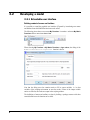
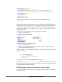
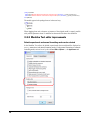
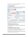
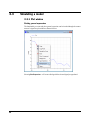
Dymola
Dynamic Modeling Laboratory
Dymola Release notes
Dymola 2013 FD01
The information in this document is subject to change without notice.
Document version: 1
© Copyright 1992-2012 by Dassault Systèmes AB. All rights reserved.
Dymola® is a registered trademark of Dassault Systèmes AB.
Modelica® is a registered trademark of the Modelica Association.
Other product or brand names are trademarks or registered trademarks of their respective holders.
Dassault Systèmes AB
Ideon Science Park
SE-223 70 Lund
Sweden
E-mail:
URL:
Phone:
Fax:
[email protected]
http://www.Dymola.com
+46 46 2862500
+46 46 2862501
Contents
1
2
3
Important notes on Dymola .................................................................................................... 5
About this booklet ................................................................................................................... 5
Dymola 2013 FD01 .................................................................................................................. 6
3.1 Introduction ...................................................................................................................................................... 6
3.1.1
Additions and improvements in Dymola ................................................................................................ 6
3.1.2
New and updated libraries ...................................................................................................................... 6
3.1.3
Limited Availability features .................................................................................................................. 7
3.2 Developing a model ......................................................................................................................................... 8
3.2.1
Extendable user interface ........................................................................................................................ 8
3.2.2
Modelica Text editor improvements ..................................................................................................... 10
3.2.3
Saving default settings improved.......................................................................................................... 11
3.2.4
Splitting models .................................................................................................................................... 12
3.2.5
Saving start values in model ................................................................................................................. 12
3.2.6
Matching and variable selections .......................................................................................................... 12
3.2.7
Minor improvements ............................................................................................................................ 18
3.3 Simulating a model ........................................................................................................................................ 20
3.3.1
Plot window .......................................................................................................................................... 20
3.3.2
Linear systems analysis ........................................................................................................................ 30
3.3.3
Scripting ............................................................................................................................................... 31
3.3.4
Selection of 32-bit or 64-bit executable ................................................................................................ 32
3.3.5
Saving start values in model ................................................................................................................. 32
3.3.6
User-defined selection what variables to be saved in the result file ..................................................... 32
3.4 Installation ...................................................................................................................................................... 34
3.4.1
Adding libraries and demos to the File menu ....................................................................................... 34
3.4.2
Borrowing 32/64 bit Dymola ................................................................................................................ 34
3.4.3
System requirements............................................................................................................................. 34
3.5 Other Simulation Environments ..................................................................................................................... 35
3.5.1
Dymola – Matlab interface ................................................................................................................... 35
3.5.2
Real-time simulation............................................................................................................................. 36
3.5.3
FMI Support in Dymola ....................................................................................................................... 37
3.6 Advanced Modelica Support .......................................................................................................................... 43
3.6.1
Synchronous Modelica and State Machines (LA) ................................................................................ 43
3.6.2
Support for String variables in models ................................................................................................. 44
3.6.3
Define class from scripting environment .............................................................................................. 44
3
3.6.4
External functions in other languages ................................................................................................... 44
3.6.5
Minor improvements ............................................................................................................................ 44
3.7 New libraries .................................................................................................................................................. 45
3.7.1
Electric Power Library.......................................................................................................................... 45
3.7.2
Engine Dynamics Library ..................................................................................................................... 46
3.7.3
Hydro Power Library ............................................................................................................................ 47
3.7.4
Liquid Cooling Library ......................................................................................................................... 48
3.7.5
Modelica_Synchronous Library (LA) .................................................................................................. 48
3.7.6
Thermal Power Library ........................................................................................................................ 49
3.8 Updated libraries ............................................................................................................................................ 50
3.8.1
AirConditioning Library ....................................................................................................................... 50
3.8.2
Hydraulics Library ................................................................................................................................ 50
3.8.3
Modelica_LinearSystems2 ................................................................................................................... 50
3.8.4
Pneumatics Library ............................................................................................................................... 50
3.8.5
PowerTrain Library .............................................................................................................................. 50
3.8.6
SmartElectricDrives Library ................................................................................................................. 51
3.8.7
Vehicle Dynamics Library.................................................................................................................... 51
3.9 Documentation ............................................................................................................................................... 51
4
1
Installation on
Windows
Important notes on Dymola
To translate models in Dymola 7.x and later you must also install a supported Microsoft
Visual Studio C++ compiler. The compiler is not distributed with Dymola. Note that free
Microsoft compiler versions earlier than Microsoft Visual Studio Express 2008 are not
supported (concerning full versions, some earlier versions are supported). Refer to section
“Software requirements” on page 34 for more information.
Administrator privileges are required for installation.
2
About this booklet
This booklet covers Dymola 2013 FD01.
The disposition is similar to the one in Dymola User Manual Volume 1 and 2; the same
main headings are being used (except for e.g. Libraries and Documentation).
Dymola 2013 FD01 Release notes
5
3
3.1
Dymola 2013 FD01
Introduction
3.1.1 Additions and improvements in Dymola
A number of improvements and additions have been implemented in Dymola 2013 FD01. In
particular, Dymola 2013 FD01 provides
• Extendable user interface; special packages can be used to define content of menus and
toolbars, enabling e.g. defining own commands and define packages with your own
collections of favorite models.
• Modelica Text editor improvements.
• More default settings can be saved between sessions, e. g. settings for the Modelica Text
editor.
• Splitting of models now also supports creating base classes.
• Saving start values in model; enabling saving initial conditions and parameter values to
the model from the variable browser.
• User-defined selections of variables to be saved in result file, simplifying postprocessing.
• Plotting general expressions.
• Signal operators in plots.
• Curves defined by parameters can be plotted using a new in-built function.
• Visualizing simulation signals as tables in addition to curves.
• Linear systems analysis improvements.
• Possibility to select whether the model should be compiled as 32-bit or 64-bit executable
on 64-bit platforms.
• A number of limited availability (LA) features are also provided; please see
corresponding section below.
3.1.2 New and updated libraries
New libraries
The following libraries are new:
• Electric Power Library, version 2.0
• Engine Dynamics Library, version 1.0
• Hydro Power Library, version 2.1
• Liquid Cooling Library, version 1.0
• Thermal Power Library, version 1.5
6
For more information about the new libraries, please see section “New libraries” starting on
page 45.
Updated libraries
The following libraries have been updated:
• AirConditioning Library, version 1,8.3
• Hydraulics Library, version 3.3
• Modelica_LinearSystems2, version 2.3
• Pneumatics Library, version 1.5.3
• PowerTrain Library, version 2.2.0
• SmartElectricDrives Library, version 1.4.2
• Vehicle Dynamics Library, version 1.7
For more information about the updated libraries, please see the section “Updated libraries”
starting on page 50.
3.1.3 Limited Availability features
This version of Dymola contains certain features which are labeled “Limited Availability”
(LA). It means that the implementation might be partial, diagnostics partial, the testing is
not complete, and no support/maintenance and only limited documentation is available.
However, we provide them to you as early as possible in order for you learn about these
features, plan for later use, and be able to give us your feedback. You typically need to set
some switch to enable them. These features are planned to become Generally Available
(GA) in the Dymola 2014 release.
Please provide any feedback to [email protected].
The following features are considered LA:
•
Synchronous Modelica and state machine support, according to the Modelica
Language version 3.3.
•
Modelica_Synchronous library
•
FMI 2.0 Beta 4 support
•
Controlling icons by parameters
The LA features are briefly described below and are marked (LA).
Dymola 2013 FD01 Release notes
7
3.2
Developing a model
3.2.1 Extendable user interface
Defining content of menus and toolbars
It is possible to extend the graphical user interface of Dymola by introducing own menus
and toolbars from which Modelica functions can be called.
The following picture shows a new menu My Functions. It contains a sub-menu My Matrix
Functions and two menu items sin and cos.
When selecting My Functions > My Matrix Functions > eigen values, the dialog of the
Modelica.Math.Matrices.eigenValues function is shown:
Note that the dialog now also contains entries to fill in output variables, i.e. in what
variables of the scripting environment to store the results. If none of the output variable
entries are filled-in, the results are output in the scripting window.
The definitions of menus and toolbars are done by defining a package structure with short
extends definitions to the functions to be called.
8
package MyFunctions "My Functions"
package MyMatrixFunctions "My Matrix Functions"
function solve=Modelica.Math.Matrices.solve(A=[1,2;3,4],b={1,1}) annotation (Icon(graphics={…}));
function eigenValues=Modelica.Math.Matrices.eigenValues "eigen values" annotation (Icon(graphics={…}));
annotation(Icon(graphics={…}));
end MyMatrixFunctions;
function sin=Modelica.Math.sin;
function cos=Modelica.Math.cos;
annotation(__Dymola_toolbar=true, __Dymola_menu=true, Protection(hideFromBrowser=true));
end MyFunctions;
Note that icon annotations have been given for solve, eigenValues and MyMatrixFunctions
and that these are used in the menus. If a description string is given, for example, “My
Functions”, “My Matrix Functions” and “eigen values”, those strings are used for the menu
otherwise the defined name. It is possible to give values to inputs which then become
prefilled in the dialog.
The package structure is made into a menu by providing the annotation
annotation(__Dymola_menu=true);
It is also possible to define a toolbar:
Toolbars are created by giving the annotation:
annotation(__Dymola_toolbar=true);
It is possible to hide such a package from the package browser by using the annotation:
annotation(Protection(hideFromBrowser=true));
Such a package can be automatically loaded by using a libraryinfo.mos file with
category=”persistent”:
LibraryInfoMenuCommand(
category="persistent",
reference="<Class To Preload>",
text="dummy")
It then not removed when the File > Clear All command is given.
The annotation __Dymola_hideGraphics=true can be used to hide the graphics coming
from the base class. This also means that the base class is only loaded when needed to build
the parameter dialog and call the function.
Defining packages with users own collection of favorite models
It is possible to define packages with your own collections of favorite models by introducing
shortcuts to models.
Dymola 2013 FD01 Release notes
9
package MyModels
model Inertia=Modelica.Mechanics.Rotational.Components.Inertia annotation (__Dymola_shortcut=true);
model Mass=Modelica.Mechanics.Translational.Components.Mass(L=1) annotation (__Dymola_shortcut=true);
end MyModels;
The models appear in the package browser in the usual way:
When dragging from such a shortcut, an instance of the original model is created, possible
with prefilled parameter values if a modifier has been used in the short class definition.
3.2.2 Modelica Text editor improvements
Default expand mode and manual formatting mode can be selected
In the Modelica Text editor, the default expand mode (how much should be displayed as
text, e.g. annotations) and manual formatting mode (if using manual formatting or automatic
formatting mode) can now be set by the command Edit > Options…, the Appearance tab:
10
A new group “Modelica editor” is added in the dialog.
The expand modes are selectable:
Manual formatting is selected by ticking the Manual formatting checkbox.
The above settings can also be saved between sessions. Please see next section.
Other improvements
• Collapsed content can be deleted, a question will be displayed whether to do it.
• Decrease of indentation using Shift+Tab.
3.2.3 Saving default settings improved
More settings can now be saved between sessions using the command Edit > Options…, the
Save Settings tab:
Dymola 2013 FD01 Release notes
11
The Save button now saves more settings in the Appearance tab (see first figure in
previous section); including the Modelica editor settings.
3.2.4 Splitting models
The creation of submodels introduced in previous version of Dymola has been extended to
also cover base classes. Selecting component/components, then right-clicking and selecting
Split Model in the context menu will display the dialog box to the left below:
Selecting Move to base class will display the dialog box to the right above. This dialog
box is used to create a base class from the selected components. You can select the
destination and if the base class should be partial.
3.2.5 Saving start values in model
Initial conditions and parameter values entered in the variable browser in simulation mode
can be saved to the model. Please see corresponding section “Saving start values in model”
on page 32 in next chapter.
3.2.6 Matching and variable selections
In order to make it easier to browse the result and parameters of large models, selections
have been introduced. It is based on pattern matching of variable names, attributes and tags.
Tags can be introduced as text annotations for variables and components.
Note that this feature can be used to decrease the size of the result file; only variables
corresponding to selections are saved by default, please see section “User-defined selection
what variables to be saved in the result file” on page 32.
12
Basic Functionality
A selection of all variables called “phi” in a model can be made using the following
annotation.
model Selection1
annotation (__Dymola_selections={
Selection(name="MySelection",
match={MatchVariable(name="*.phi")})});
end Selection1;
The selection feature can be activated by extending the model containing the selections
annotation:
model MyFullRobot
extends Modelica.Mechanics.MultiBody.Examples.Systems.RobotR3.fullRobot;
extends Selection1;
end MyFullRobot;
It results in the following content of the variable browser:
In addition to the selection, parameters and states are preselected.
Introducing New Names
The MatchVariable has an attribute newName. When newName is used, the variable is
included in a new subtree with the name of the selection. To use the same variable name as
before one can use newName="%componentPath%%name%" or alternatively %path%.
model Selection2
annotation (__Dymola_selections={
Selection(name="MySelection",
match={MatchVariable(name="*.phi", newName="%path%")})});
end Selection2;
It results in the following additional content of the variable browser:
Dymola 2013 FD01 Release notes
13
Including several variables in the selection can be made by using | in the regular expression
for name:
model Selection3
annotation (__Dymola_selections={
Selection(name="MySelection",
match={ MatchVariable (name="*.(phi|tau)", newName="%path%")})});
end Selection3;
Resulting in:
Alternatively of using |, several matchings can be used. They are or’ed.
model Selection4
annotation (__Dymola_selections={
Selection(name="MySelection",
match={ MatchVariable (name="*.phi", newName="%path%"),
MatchVariable (name="*.tau", newName="%path%")})});
end Selection4;
It is possible to build subtrees, by including a subtree name in the newName path:
14
model Selection5
annotation (__Dymola_selections={
Selection(name="MySelection",
match={ MatchVariable (name="*.phi", newName="Angles.%path%")}),
Selection(name="MySelection",
match={ MatchVariable (name="*.tau", newName="Torgues.%path%")})});
end Selection5;
resulting in
Matching within a scope
It can be noted that the annotation in model Selection2 gave the result:
Dymola 2013 FD01 Release notes
15
i.e. the local variable phi of angleSensor is present. The reason was that the search pattern
given was “*.phi”, i.e. any prefix to .phi. The pattern matching is performed from the top
level model so the path “axis1.angleSensor.phi” was found. It is possible to make the pattern
matching locally in certain classes only, by providing a (pattern for the) class name. In this
case the pattern for the name is just “phi”.
model Selection6
annotation (__Dymola_selections={
Selection(name="MySelection",
match={MatchVariable(className="Modelica.Mechanics.Rotational.Interfaces.Flange*",
name="phi", newName="%path%")})});
end Selection6;
The result is then:
Tags
Variables can be tagged using the tag annotation:
Real w annotation(__Dymola_tag={"Mechanical"});
Several tags can be associated with a variable:
Real w annotation(__Dymola_tag={"Mechanical","Rotational"});
If a tag is attached to a component, it is also attached to sub-components and variables.
Matching can then be made on tags as well.
Advanced Pattern Matching and Substitution
All matches must be exact, and only scalar variables are considered for the matching;
however, tags are inherited by sub-components.
The regular expression syntax is the same as in the Advanced plot dialog.
The name, description, and tag support leading “!” for selecting non-matches.
The newName can use %componentPath%, %name%, %path% and %i%. The %name%
corresponds to the part matching the regular expression and %componentPath%%name% is
the full path of the variable. The %1% is the part matching the first parenthesis-enclosed
part of the regular expression.
16
Summary
The matching constructor MatchVariable has the following fields:
record MatchVariable
String className="" "Classes to look in";
String name="*" "Regular expression for variable name";
String description="" "If non-empty, regular expressions that should exactly match description";
String tag[:]=fill("",0) "If non-empty, regular expressions that should exactly match any tag";
String newName ="" "New name";
end MatchVariable;
Regular expressions can be used in all fields.
The selection constructor is:
record Selection
String name;
MatchVariable match[:];
Boolean override=false;
end Selection;
Selection annotations can be included in several models not only on the top level. The
override attribute determines if selections with the same name found on lower hierarchical
levels of the model should be overridden or merged.
User Interface
In the variable browser, it is possible to get a list of all selections and marking which of
those selections that should be included in the variable tree:
The selection Parameters and States is predefined corresponding to the interactive fields
for setting parameters and initial conditions of states.
If several selections have been defined:
model Selection7
annotation (__Dymola_selections={
Selection(name="Angles",
match={MatchVariable(name="*.phi", newName="%path%")}),
Selection(name="Torques",
match={MatchVariable(name="*.tau", newName="%path%")})});
end Selection7;
Dymola 2013 FD01 Release notes
17
they can be activated or deactivated individually:
3.2.7 Minor improvements
Search in model package hierarchy
The search engine used in the command File > Search… and the corresponding context
menu entry Search… is now enhanced to allow regular expressions in all fields. To use
regular expressions, the checkbox Regular expression search in the Search options
group in the dialog box should be ticked.
Special symbols in the regular expressions are:
*
Match everything.
?
Match any single character.
{ab}
Match characters a or b.
{a-z}
Match characters a through z.
{^ab}
Match any characters except a and b.
E+
Match one or more occurrence of E.
(ab|cd)
Match ab or cd.
\d
Match any digit.
\w
Match any digit or letter.
^
Match from start.
$
Match at end.
Tooltip displaying type error for components in diagram layer
The tooltip will now display the type when there is a type error (box with red cross).
18
Presentation of enumeration values
If an enumeration is used for a parameter, a combo box is created in the parameter dialog. If
only enumeration values should be used (and not parameter propagation) the annotation
annotation(__Dymola_editText=false)
can be used. In such case only the selected value of the enumeration is shown in the input
field, not the entire path including the name of the type.
Controlling icons by parameters (LA)
If a parameter expression is used as the second argument of DynamicSelect, and the
expression can be evaluated, it is used also in Edit mode. First argument of DynamicSelect
is used in case of failure. References to submodel parameters are also allowed. This feature
is enabled with Advanced.ActivateParameterValuesInDiagram=true.
Not expanding declarations
Declarations of several variables in one declaration are not expanded by the Modelica editor
any longer.
Checking annotations
The pedantic mode which can be set in the Simulation setup/Translate tab gives warnings
about non-recognized annotations when giving the Check command.
Pressing SHIFT to set aspect ratio 1:1
Holding down SHIFT will keep the aspect ratio 1:1 when drawing rectangles, ellipses, texts
and bitmaps.
Dymola 2013 FD01 Release notes
19
3.3
Simulating a model
3.3.1 Plot window
Plotting general expressions
The functionality to create and plot a general expression can be invoked through the context
menu of a signal in a plot window as shown in below:
Selecting Plot Expression… will create a dialog with the selected signal pre-populated:
20
Note that the name of the signal also contains the name of the result and the sequence
number (in brackets). The identifiers end and end-1 are generated for the latest and second
latest results; in other cases the absolute sequence number of the result is generated.
The expression in the dialog can then be created by a combination of manual editing and by
selecting other signals from the variable browser. When a signal is selected, the name of the
signal is automatically generated in the Plot expression dialog at the current position of the
cursor. An example is shown below:
After pressing OK, the expression is parsed, and if valid it is plotted in the active plot
window. By default, the entered expression is also shown in the legend of the plot window.
The legend can be changed by entering a different string in the Legend field of the Plot
expression dialog.
Dymola 2013 FD01 Release notes
21
Alternative ways of invoking this function is through the command Plot expression in the
Dymola toolbar, or by the command Plot > Plot Expression….
Since the function is not invoked on a signal, the Plot Expression dialog will not contain
any pre-populated signal in this case:
The “Plot expression” functionality has support in the scripting environment through the
function plotExpression. This function can, for example, be used to change the default
legend generated for an expression in a plot window.
It is also possible to combine signals from different result files when building the
expression. As shown already above, the notation used to indicate the result file is
resultFile[resultID], see the example below:
22
Signal operators
A fixed set of signal operators are available through the context menu of signals in plot
windows. The operators are applied over a user-defined time range, and the following
operators are available:
• Minimum and maximum value
• Slew rate
• Arithmetic and rectified mean
• Root-mean-square (RMS)
• AC-coupled RMS
• First harmonic
• Total harmonic distortion (THD)
The Signal Operator selection in the context menu is shown below:
Dymola 2013 FD01 Release notes
23
Selecting an operator launches a dialog where the user can define the time range over which
the operator will be applied. The default time range is from the start time to the stop time of
the simulation. For the operators First Harmonic and Total Harmonic Distortion, the
period of the signal must be entered.
An error message is raised if the specified time range is out of bounds or if the minimum is
larger than the maximum.
24
The result is then visualized in the plot in different ways depending of which operator that
was selected. The time range and the associated text are using black color by default. If the
plot contains more than one curve the text is written in the same color as the plotted signal.
The picture below shows the appearance of all available operators:
Common for all cases is that the time range is represented with a horizontal line with clearly
marked end points. It is possible to interactively change the range by drag-and-drop of the
end points or by moving the whole line (keeping the range fixed). It is also possible to mark
and then delete a time range and the associated operator.
Dymola 2013 FD01 Release notes
25
Depending on the operator, the computed value is written either above or below the line
representing the time range. This can be changed manually using the command Label
Above Line in the context menu of the time range:
Using this context menu you can also copy the value of the signal operator to the clipboard.
The “Signal Operator” functionality has support in the scripting environment (except for
First
Harmonic
and Total Harmonic Distortion) through the function
plotSignalOperator, for example:
plotSignalOperator("J1.a",SignalOperator.ACCoupledRMS,0.3,0.7);
26
Plot Parametric Curve
A new function plotParametricCurve is available for plotting curves defined by a
parameter:
function plotParametricCurve "plot parametric curve"
input Real x[:] "x(s) values";
input Real y[size(x, 1)] "y(s) values";
input Real s[size(x, 1)] "s values";
input String xName = "" "The name of the x variable";
input String yName = "" "The name of the y variable";
input String sName = "" "The name of the s parameter";
input String legend = "" "Legend describing plotted data";
input Integer id = 0 "Identity of window (0-means last)";
input Integer color[3] = {-1, -1, -1} "Line color";
input Integer pattern = 2 "Line pattern, e.g., LinePattern.Solid";
input Integer marker = -1 "Line marker, e.g., MarkerStyle.Cross";
input Real thickness = 0.25 "Line thickness";
input Boolean labelWithS = false "if true, output values of s along the curve";
input Boolean erase = false "Erase window content before plotting";
output Boolean result "true if successful";
// Makes a x(s) - y(s) plot of given values.
end plotParametricCurve;
Giving the commands:
s=0:0.1:10
y={sin(t)*exp(-0.1*t) for t in s}
x={cos(t)*exp(-0.1*t) for t in s}
plotParametricCurve(x, y, s, labelWithS=true);
produces the following plot
The labels can be turned on and off in the context menu of the curve:
Dymola 2013 FD01 Release notes
27
Copy curve values to clipboard
The values of a curve can be copied to the clipboard by the Copy context command.
As an example, copying J1.w:
and paste into Microsoft Excel will result in (the figure showing only the first values):
28
(The previous copy command for copying the tooltip to the clipboard has been renamed to
Copy Point.)
Plot table
In Dymola 2013 FD01 a plot can be displayed as a table instead of a curve. To create a plot
table, select the command Plot > New Window > New Table Window.
In the below example, a table has been displayed with the same signals selected as in the
curve plot.
Right-clicking in the table displays a context menu:
Dymola 2013 FD01 Release notes
29
Copy copies the selected cells to the clipboard, making it possible to e.g. copy a part of a
table to Microsoft Excel.
Delete Row deletes the selected row(s). A row can also be deleted by deselecting the
corresponding signal in the variable browser.
Copy Entire Table copies the entire table to the clipboard.
Erase All erases all table values.
3.3.2 Linear systems analysis
A new menu Linear analysis is available with shortcuts to certain functions in the
Modelica_LinearSystems2 library:
Below the functions are described very short, for further information please refer to the
documentation of the library.
• Linearize - Linearize a model and return the linearized model as StateSpace object.
• Poles - Linearize a model and plot the poles of the linearized model.
• Poles and Zeros – Linearize a model and plot the poles and zeros of the linearized
model.
• Transfer functions - Linearize a model and plot the transfer functions from all inputs to
all outputs of the linearized model.
• Full linear analysis - Linearize a model and perform all available linear analysis
operations.
• Root locus - Compute and plot the root locus of one parameter of a model (=
eigenvalues of the model that is linearized for every parameter value).
30
3.3.3 Scripting
Call function dialog with output fields
The Call function dialog now also contains entries to fill in output variables, i.e. in what
variables of the scripting environment to store the results. If none of the output variable
entries are filled-in, the results are output in the scripting window.
Delete variables in workspace
The function deleteVariables can be used to delete variables in work space
function deleteVariables
input String variables[:];
output Integer nrDeleted;
end deleteVariables;
Example:
deleteVariables({"A", "B"});
Script support for signal operators
The signal operator feature is also supported (except for the operators First Harmonic and
Total Harmonic Distortion) in the built-in function plotSignalOperator(); see the
section about signal operators above.
Script support for plot expressions
The plot expression feature described above is also supported in the built-in function
plotExpression(); see the section about plotting expressions above.
Dymola 2013 FD01 Release notes
31
3.3.4 Selection of 32-bit or 64-bit executable
In the 64-bit version of Dymola, the user can decide whether models should be compiled as
32-bit or 64-bit executables, using the flag Advanced.CompileWith64. The flag has three
possible values:
• 0
(default value); dymosim.exe compiled as 32-bit, dymosim.dll, dymosim as DDE
server, and FMUs compiled as 64-bit.
• 1
All applications above compiled as 32-bit
• 2
All applications above compiled as 64-bit
Dymosim as OPC server can presently only be compiled as 32-bit, setting
Advanced.CompileWith64=2 is not supported when compiling dymosim as OPC server.
3.3.5 Saving start values in model
Modified initial conditions and parameter values entered in the variable browser in
simulation mode can be saved to the model typically after being validated by a simulation,
by right-clicking the result file in the variable browser and selecting Save Start Values in
Model.
3.3.6 User-defined selection what variables to be saved
in the result file
A new annotation enables defining what categories of variables that should be saved in the
result file. See section “Matching and variable selections” starting on page 12 for more
information.
This feature is very valuable when having a large model with many variables, but only being
interested in a selection of variables.
Whether only selected variables should be saved in the result file is decided by the setting
All variables; ignore selections in model, a setting displayed using the command
Simulation > Setup…, selecting the Output tab.
32
Ticking All variables; ignore selections in model, all variables, given the Store settings,
will be saved to the result file. If not ticked (default), only selected variables, given the
Store settings, will be saved to the result file.
If no selections are available, the value of the flag has no effect.
To clarify what is actually stored, this setting, and the setting Protected variables setting,
have been put in a new group: Store additional variables. This clarifies that these settings
are additional storage settings compared with the settings in the group Store.
Note that these settings in default state decrease the number of variables being saved. If
both settings are ticked, variables according to the Store group settings are being saved.
Unticking any of them decrease the number of variables saved; e.g. Protected variables
being unticked, a filter is applied on the variables to be saved according to the Store group
settings, excluding protected variables from being saved.
Dymola 2013 FD01 Release notes
33
3.4
Installation
3.4.1 Adding libraries and demos to the File menu
A new category “persistent” in the built-in function LibraryInfoMenuCommand makes it
possible to automatically load a package containing user-defined menus and toolbars using a
libraryinfo.mos file. Such menus and toolbars will not be removed by the File > Clear
All command. For an example, see section “Defining content of menus and toolbars” on
page 8.
3.4.2 Borrowing 32/64 bit Dymola
When borrowing only the Dymola version you run will be borrowed: and 64-bit and 32-bit
Dymola are seen as different versions. For the few cases where you want to
• Borrow a license, AND
• run Dymosim.exe outside of Dymola, AND
• do not have export option;
we advice that you in 64-bit Dymola generate a 64-bit Dymosim.exe using the flag
Advanced.CompileWith64=2. See section “Selection of 32-bit or 64-bit executable” on
page 32 for more information.
3.4.3 System requirements
Hardware requirements
• At least 1 GB RAM
• At least 400 MB disc space
Hardware recommendations
At present, it is recommended to have a system with an Intel Core 2 Duo processor or better,
with at least 2 MB of L2 cache. Memory speed and cache size are key parameters to achieve
maximum simulation performance.
A dual processor will be enough; the simulation itself uses only one execution thread so
there is no need for a “quad” processor.
Memory size may be significant for translating big models and plotting large result files, but
the simulation itself does not require so much memory. Recommended memory size is 2-4
GB of RAM for 32-bit architecture and 3-6 GB of RAM for 64-bit architecture.
Software requirements
Microsoft Windows
On Windows, Dymola 2013 FD01 is supported, as 32 or 64 bit application, on Microsoft
Windows XP, Windows Vista and Windows 7. Since Dymola does not use any features
34
supported only by specific editions of Windows (“Home”, “Professional”, “Enterprise”
etc.); all such editions are thus supported if the main version is supported.
For the Windows platform, Microsoft C/C++ compiler must be installed separately. The
following compilers are supported for Dymola 2013 FD01 on Windows:
Free editions:
• Visual Studio 2008 Express Edition (9.0)
• Visual C++ 2010 Express (10.0)
Professional editions:
• Visual Studio 2005 (8.0)
• Visual Studio 2008 (9.0)
• Visual Studio 2010 (10.0)
Linux
On Linux, Dymola 2013 is supported on Red Hat Enterprise 5.1 with gcc version 4.1.1, and
compatible systems (32 bit). Please note that multi-criteria design optimization is not
supported on Linux. There is no native Dymola 64 bit application for Linux.
3.5
Other Simulation Environments
3.5.1 Dymola – Matlab interface
UTF-8 support
The UTF-8 support that was introduced in Dymola 2013 is now also available in the
Simulink interface. Description strings (including units) of parameters and start values are
now rendered with the correct Unicode characters in the DymolaBlock GUI.
Support for expandable bus connectors
The Dymola kernel and the Simulink interface have been improved to fully support export
of models containing expandable bus connectors to Simulink. Inputs and outputs that are
propagated to the top level of a model using expandable bus connectors are now
automatically converted to inputs and outputs of the corresponding Simulink block. The
expandable connectors can also be mapped to Simulink bus signals.
Simulink interface updated on Linux
The documentation of the Simulink interface on Linux has been updated to more clearly
describe the two-step export/import procedure. The export step uses the library
ExternalInterfaces 1.2.1 available in the Dymola/Modelica/Library folder of the Dymola
installation.
Dymola 2013 FD01 Release notes
35
Compatibility
The Dymola – Simulink interface now supports Matlab releases from R2007a (ver. 7.4) up
to R2012a (ver. 7.14). Only Visual Studio C++ compilers are supported to generate the
DymolaBlock S-function. The LCC compiler is not supported.
Note: Matlab R2010bSP1, R2011a, R2011b, and R2012a will give warnings that files in the
Dymola/Mfiles folder are generated with an old p-code version. These warnings are
uncritical and can be turned off by adding the following line to your Matlab startup script:
warning('off', 'MATLAB:oldPfileVersion');
3.5.2 Real-time simulation
Improved code generation
The Dymola code generation has been improved to support modern versions of the GCC
compiler. Especially, GCC versions 4.x that are used for various real-time targets through
Real-Time Workshop / Simulink Coder are now fully supported.
Compatibility – dSPACE
Dymola 2013 FD01 generated code has been verified for compatibility with the following
combinations of dSPACE and Matlab releases on the DS1005 and DS1006 platforms
• dSPACE Release 5.4 (RTI 5.5) with Matlab R2007a
• dSPACE Release 6.0 (RTI 5.6) with Matlab R2007b
• dSPACE Release 6.1 (RTI 6.0) with Matlab R2007b
• dSPACE Release 6.2 (RTI 6.1) with Matlab R2008a
• dSPACE Release 6.3 (RTI 6.2) with Matlab R2008b
• dSPACE Release 6.4 (RTI 6.3) with Matlab R2009a
• dSPACE Release 6.5 (RTI 6.4) with Matlab R2009b
• dSPACE Release 6.6 (RTI 6.5) with Matlab R2010a
• dSPACE Release 7.0 (RTI 6.6) with Matlab R2009bSP1, R2010b, and R2010bSP1
• dSPACE Release 7.1 (RTI 6.7) with Matlab R2011a
• dSPACE Release 7.2 (RTI 6.8) with Matlab R2011a and R2011b
• dSPACE Release 7.3 (RTI 6.9) with Matlab R2011a, R2011b, and R2012a
The selection of supported dSPACE releases focuses on releases that introduce support for a
new Matlab release and dSPACE releases that introduce a new version of a cross-compiler
tool. In addition, we always support the three latest dSPACE releases with the three latest
Matlab releases. Although not officially supported, it is likely that other combinations
should work as well.
36
Compatibility – xPC Target
Compatibility with Matlab xPC Target has been verified for all Matlab releases that are
supported by the Dymola – Simulink interface, which means R2007a (xPC Target ver. 3.2)
to R2012a (xPC Target ver. 5.2). Only Microsoft Visual C compilers have been tested.
3.5.3 FMI Support in Dymola
64-bit export and import of FMUs
Dymola 2013 FD01 64-bit version now supports both export and import of 64-bit FMUs.
Exporting an FMU using the 64-bit version of Dymola will create both 32-bit and 64-bit
binaries if possible. Note that compiling applications (dymosim.exe) that contain imported
64-bit FMUs requires setting the flag
Advanced.CompileWith64 = 2
See detailed description of this flag in section “Selection of 32-bit or 64-bit executable” on
page 32 above.
FMU export
Improved user interface for FMI export settings
Commands and settings related to FMI export have been collected into one tab in the
simulation setup, reached by the command Simulation > Setup…, or by the Setup button,
the FMI Export tab:
Dymola 2013 FD01 Release notes
37
For description of the new options, see below, section “FMU export extensions”.
FMU export extensions
FMUs can optionally be exported with source code included, by setting the new Boolean
argument
includeSource = true
in translateModelFMU.
This function has also become more explicit in that its complete behavior is controlled via
arguments instead of global flags. The new string argument
fmiType
38
can be set to “me”, “cs” and “all” for inclusion of “model exchange”, “co-simulation” and
“all” respectively.
In addition, the new string argument
fmiVersion
controls the FMI verision (“1” or “2”) of the FMU. For FMI 2.0, see below.
The default values for the new arguments to translateModelFMU are chosen in a backward
compatible manner; old calls to it will behave the same except that fmiType defaults to “all”
instead of “me”.
Finally, for result storing (argument storeResult = true), the result file is named
according to the instance name chosen during FMU initialization, <instance name>.mat,
instead of the generic “dsres.mat”.
Note that Dymola does no longer generate any static import library in the binaries folder
when exporting an FMU, see also section “No import library required in imported FMU”
above.
FMU Export on Linux
The FMU export on Linux requires the Linux utility “zip”. If not already installed, please
install using your packaging manager (e.g. apt-get) or see e.g. http://info-zip.org.html.
Updated FMU export from Simulink
The package to generate FMUs from Simulink models (Dymola/Mfiles/rtwsfcnfmi.zip) has
been updated. The main changes are
• MATLAB support for releases R2007 to R2011b
• Support for 64-bit MATLAB installations
• Support for Visual Studio 2010 compiler
See the README file contained in the package for details and updated installation
instructions.
FMU import
No import library required in imported FMU
The previous restriction that imported FMUs needed to have a static import library in the
binaries folder (in addition to the DLL) is now removed. Also, no such libraries are
generated by Dymola when exporting an FMU.
Repeated import of FMU by scripting improved
A new argument promptReplacement has been added to the importFMU function:
importFMU(fileName, includeAllVariables, integrate,
promptReplacement)
Dymola 2013 FD01 Release notes
39
This argument, default being true, can be set to false to disable the prompting before
replacing any existing Modelica model that was the result from a previous import. This is
useful for scripting.
Import of FMUs for Co-Simulation 1
The Co-Simulation FMU import is enabled by setting the input argument integrate of the
function importFMU to false. The macro step size can be set as the parameter
fmi_CommuncationStepSize in the FMI tab in the parameter dialog of the generated
Modelica model. The default macro step size is (stop time – start time)/500. Refer to the
next section for details.
Validating FMUs
Once the dynamic behavior of a model is verified and it is ready to be exported as FMU, one
would like to verify that this behavior can be repeated on the targeted simulation
environment. For model exchange, which is dependent on the solver of the target, this is
naturally less straight-forward than for co-simulation, where the solver is built into the
FMU. We focus this discussion on the co-simulation case, although all is possible for model
exchange as well.
Normally, the FMU contains inputs that need to be connected to signal generators (sources)
before this validation can be commenced. Since this is model and test dependent and hard to
automate, we will assume the model inputs have been connected to necessary sources
beforehand. The result is a test model with no disconnected inputs. After the validation,
these sources are of course removed before the final FMU is created.
Since Dymola supports FMU import, it becomes natural to re-import the FMU in Dymola
and compare its simulation with the original model. We demonstrate this for the demo
model CoupledClutches. For brevity and since not all import options are yet available in the
GUI, we use a scripting perspective. First, export as FMU with, say, both model exchange
and co-simulation support:
translateModelFMU(
"Modelica.Mechanics.Rotational.Examples.CoupledClutches",
false, "", "1", "all");
Re-import, in a non-interactive mode, the FMU for co-simulation:
importFMU(
"Modelica_Mechanics_Rotational_Examples_CoupledClutches.fmu",
true, false, false);
Simulate the model being the result of the import:
simulateModel(
"Modelica_Mechanics_Rotational_Examples_CoupledClutches_fmu",
stopTime=1.5, method="dassl");
1
The import of FMUs for Co-Simulation functionality is currently intended for validating export of Co-Simulation
FMUs created in Dymola by re-importing them to Dymola. Importing Co-Simulation FMUs from other vendors has
not been tested due to no such FMUs being currently available.
40
Finally, the resulting trajectories can be plotted and compared visually with the original
(non-FMU) simulation. Note that, since the imported model is flattened, the trajectory
names are somewhat different; e.g. J1.w becomes J1_w:
The blue trajectory is from the reference simulation and the red is from the co-simulation.
Note that the latter is rendered as constant between the sample points.
While this validation is ok for sample testing of a single model, this clearly becomes
infeasible for systematic validation of several trajectories.
The remedy is a new function validateModelAsFMU, which automates the following
steps:
• Generation of reference trajectories.
• Exporting of the FMU.
• Importing of the FMU.
• Mapping of trajectories names to those of the original model.
• Numeric comparison of trajectories.
• Graphical HTML presentation of deviating trajectories in fashion similar to the plot
above.
Main features include:
• Using a default set of trajectories to compare or specifying it explicitly. The default it the
set of all state candidates.
• Choosing tolerance for the comparison.
• Optional generation of reference trajectories which is typically only needed once.
• Optional FMU export which might not be needed each time.
• Test of co-simulation or model exchange.
Dymola 2013 FD01 Release notes
41
•
Test of FMI version 1.0 or 2.0 Beta4.
It is available in Modelica\Library under the Dymola installation.
Below call validates CoupledClutches as a co-simulation FMU for FMI 1.0:
validateModelAsFMU(
"Modelica.Mechanics.Rotational.Examples.CoupledClutches");
An excerpt from the log file is given below:
In this case we may argue that the comparison tolerance should be increased to avoid the
report of this trajectory.
FMI 2.0 Beta 4 (LA)
Partial support is provided for FMI 2.0 Beta 4. By setting the global flag
Advanced.FMI.Version2 = true
the option of choosing FMI version 2 is enabled in the GUI (using the command Simulation
> Setup…, the FMI Export tab) for FMU export.
42
All mandatory features are supported in FMI 2.0 Beta 4. The optional (in the sense that they
have associated capability flags) features not supported are:
• FMUs can only be instantiated once per process.
• The internal FMU state cannot be serialized.
• Estimates of output derivatives are not provided.
•
fmiDoStep cannot run asynchronously.
The Files > Import > FMU… commands and script function importFMU accepts FMUs
created according to FMI 2.0 Beta 4 Model Exchange specification. Current supported
features are the same as for FMI 1.0.
3.6
Advanced Modelica Support
3.6.1 Synchronous Modelica and State Machines (LA)
The synchronous features and state machines of Modelica 3.3 have Limited Availability
(LA) support since the specification in Modelica 3.3 has been finished only recently. The
features are enabled by the scripting command Advanced.Synchronous = true.
References to papers describing these features, and a tutorial presentation, are available
using the command Help > Documentation. A tutorial is also available using the command
Help > Demos > Synchronous Tutorial. The tutorial relates to the papers and presentation
mentioned.
Dymola 2013 FD01 Release notes
43
3.6.2 Support for String variables in models
String variables can now be used in models, not only in functions used in models and for
scripting. String variables in model are allocated with a maximum string length. It is defined
by the scripting variable Advanced.MaxStringLength with default=500. If assignment to
a string variable in a model fails because of the string being too short, truncation is done and
a warning is given in the simulation log window.
String variables cannot be used in models which are exported as FMUs.
3.6.3 Define class from scripting environment
The function Dymola_AST_SetClassText can be used to create a class by scripting.
function Dymola_AST_SetClassText
input String parentName;
input String fullText;
output Boolean ok;
end Dymola_AST_SetClassText;
Giving the following commands creates the usual “Hello world” result:
Dymola_AST_SetClassText("", "function Hello output String s=\"Hello
world\"; algorithm end Hello;");
= true
Hello()
= "Hello world"
The class appears in the package browser and can be used as any other class.
The function will in the next Dymola version also be available as a corresponding function in the
ModelManagement package.
3.6.4 External functions in other languages
Java support extended
The Java interface is now also supported in Linux 32 bit. Note that on Windows only
Windows 32-bit is currently supported.
3.6.5 Minor improvements
•
•
•
44
Support of annotation(singleInstance=true) according to Modelica 3.3
specification. This feature is useful for state machines.
Support of Modelica assert with “level” argument, as described in specification.
Introduced annotation for functions to force translation (for speed-up) not only of
external functions annotation(__Dymola_translate=true)
3.7
New libraries
3.7.1 Electric Power Library
Electric Power Library is a new library that provides a framework for efficient modeling,
simulation and analysis of electric power systems. The models can be used for simulation of
steady state as well as transient operation of power systems. The multi-domain modeling
capability of Dymola makes it possible to model the complete power plant from the energy
source, whether it is oil, gas, hydropower or another renewable source such as wind, all the
way through generator and power grid to the end consumer.
The components in the Electric Power Library provide standardized interfaces to the thermal
and mechanical domains and can easily be combined with components from other libraries
to represent electric power and actuation. Applications include electric power plants and
grids, hybrid vehicles, ships, and more. It is also well suited for control design and supports
different reference frame representations.
Dymola 2013 FD01 Release notes
45
3.7.2 Engine Dynamics Library
Engine Dynamics Library is a new library that a framework for combustion engine system
modeling, simulation and analysis, including the complete gas exchange. The library is well
suited to represent transient engine response and related engine control. Applications
include control design with the purpose of reducing emission transients from the engine,
transient exhaust condition modeling for optimum EATS operation conditions, and engine
response dynamics.
The Engine Dynamics Library utilizes a mean value combustion model for torque, charge
flow and exhaust condition modeling. Pressure and thermal dynamics of the complete air
gas exchange process can be studied. Several turbo charger and EGR configurations can be
modeled, including variable geometry turbine designs.
46
3.7.3 Hydro Power Library
The Hydro Power Library is a new library that provides a framework for modeling and
simulation of hydropower plant operation. The library components enable performance
analysis and optimization of the operation of hydropower plants. It offers an excellent
environment for testing new control strategies and tuning plant controllers for optimal
performance. Optimization of the operation of power plants with multiple reservoirs and
multiple turbines in order to maximize the overall efficiency is in important application.
Accurate simulation results can have a significant effect on the efficiency and thereby the
profitability of the operation.
The Hydro Power Library is suitable for simulation of transient operation such as load
rejection to verify that the control system can handle these situations. It can also be used for
studying various control strategies to cope with the rapid load changes that become more
frequent as other renewable, less controllable, sources of energy are increasingly used for
power generation. It is also targeted for use in design of new hydropower plants. Planning of
commissioning tests and procedures can be set-up, thereby reducing the risk of unexpected
events and minimizing costly tests done on the actual plant.
Dymola 2013 FD01 Release notes
47
3.7.4 Liquid Cooling Library
The Liquid Cooling Library is a new library is targeted to liquid cooling system design with
compressible or incompressible flow. It is suitable for a broad range of applications,
including automotive, industrial equipment and process industry. Applications include
engine cooling, battery thermal management, and cooling of power electronics and
machines.
It is suited for pump dimensioning, control of thermal transient response and can be used
together with geometry based heat exchanger models. Users can connect components freely
as they desire, which makes it is easy to realize non-standard circuits.
3.7.5 Modelica_Synchronous Library (LA)
The library Modelica_Synchronous is a Modelica package to precisely define and
synchronize sampled data systems with different sampling rates. The library has elements to
define periodic clocks and event clocks that trigger elements to sample, sub-sample, supersample, or shift-sample partitions synchronously. Optionally, quantization effects,
computational delay or noise can be simulated. Continuous-time equations can be
automatically discretized and utilized in a sampled data system. The sample rate of a
partition needs to be defined at one location only. All Modelica libraries designed so far for
sampled
systems,
such
as
Modelica.Blocks.Discrete
or
Modelica_LinearSystems2.Controller
are
becoming
obsolete
and
instead
Modelica_Synchronous should be utilized instead.
48
3.7.6 Thermal Power Library
The Thermal Power Library provides a framework for modeling and simulation of thermal
power plant operation. The comprehensive set of components enables performance analysis
and optimization of all kinds of thermal power plants. Different plant designs and their
respective dynamic behavior can be studied already in the concept design phase. The
Thermal Power Library is also well suited for control system development and verification,
e.g. to ensure that the power plant can cope with the rapid load changes that become more
frequent as renewable sources of energy are increasingly used for power generation.
It is suitable for simulation of transient operation such as start-up and load rejection to verify
that the control system handles these scenarios accordingly. A particular advantage is the
ability to simulate dynamic as well as steady-state behavior using the same model. In
addition to covering the entire steam cycle, the Thermal Power Library can also be used for
modeling and simulation of the flue gas side including a wide range of after-treatment
technologies such as desulphurization, NOx-removal and CCS.
Dymola 2013 FD01 Release notes
49
3.8
Updated libraries
3.8.1 AirConditioning Library
A minor version, 1.8.3, has been released, with some modifications, e.g.
• Dialog annotations added to variables in summary records.
• Outlet enthalpy h_out in heat exchangers now always corresponds to the state in the last
control volume independent of flow direction.
• Compressor outlet enthalpy guarded against very high values at low efficiencies.
3.8.2 Hydraulics Library
Hydraulics 3.3 is a minor release with some improvements:
• Increased numerical robustness by introducing the absolute pressure to be the preferred
choice of state.
• Example models now have fully-specified initial conditions, no longer relying on tool
dependent settings.
• Improved dialog for Cylinders.
• Parameterized minimum dead volumes, and parameterized settings for stroke limitations
in Cylinders.
Note that for readability reasons, the absolute pressures in the properties have been renamed
to p_abs and are defined as SIunits.AbsolutePressure. This may require updates in existing
modules. The conversion script should take care of this.
3.8.3 Modelica_LinearSystems2
This release, version 2.3, is a major release; backward compatible to the previous version
2.2. It contains the following main improvements (and several minor ones):
• New package "Modelica_LinearSystems2.ModelAnalysis" that contains several
functions to linearize a model and perform a selected linear analysis operation, like
plotting of poles, zeros or transfer functions.
• New plot functions in package "Modelica_LinearSystems2.Utilities.Plot" to plot
parameterized curves, as well as to plot a root locus of a model, by linearizing a model
for a set of selected parameter values.
• A new function "Modelica_LinearSystems2.Utilities.Import.linearize2" to linearize a
model and return a StateSpace object.
3.8.4 Pneumatics Library
A minor version, 1.5.3, has been released; with fully-specified example models.
3.8.5 PowerTrain Library
A new version, 2.2.0, is available. Some examples of features:
50
•
•
•
•
All physical models that dissipate heat (such as gears, clutches or dampers), have now an
optional heat port to which the dissipated energy is flowing, if activated.
Improved functionality of torque division for controllers of (hybrid) electric vehicles.
Upgraded documentation of controllers, converters, and electric drives.
Redesigned visualization elements to be compatible with those used in Modelica
Standard Library.
The version is backward compatible to PowerTrain 2.0.x.
3.8.6 SmartElectricDrives Library
Version 1.4.2 is a minor version with changes to avoid numerical problems of flux position
detection at zero flux.
3.8.7 Vehicle Dynamics Library
Version 1.7 is a major maintenance release with many changes in the underlying Modelica
code to ensure better compliance to the Modelica Language Specification (version 3.2).
Some example experiments, e.g. ParameterIdenfication and DoubleLaneChangeVerification
in SingleTrack, are now modified to take advantage of the Modelon.DataAccess architecture
that allows users to conveniently populate the models with data from sources outside the
Modelica environments.
Commands have been added to many experiments to modify the animation view in the
active animation window. The commands allow the user to quickly view a vehicle, chassis
or suspension from the front, side, rear, top or isometric perspective. Most of the example
experiments within Vehicle Dynamics Library have these commands available.
3.9
Documentation
In the software distribution of Dymola 2013 FD01 Dymola User Manuals of version
“September 2013” will be present; these manuals include all relevant features/improvements
of Dymola 2013 FD01 presented in the Release notes. Limited Availability (LA) features
are not included.
Dymola 2013 FD01 Release notes
51