Download Combi Flash EX Specifications

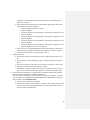
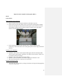
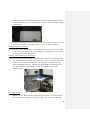
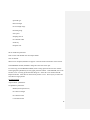
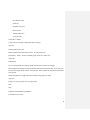
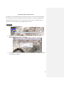
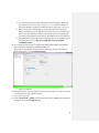
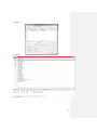
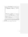
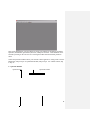
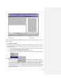
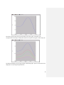
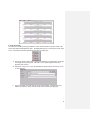
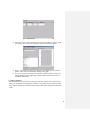
Table of Contents
1.
2.
3.
4.
5.
6.
7.
AFM/Bruker
AFM/Asylum
CombiFlash
Contact Angle
Delsa Nano AT&C
Dynamic Light Scattering
Differential Scanning Calorimetry (DSC)
7.1.
Flash DSC
8. Fourier Transform Infrared Spectrophotometer (FTIR)
9. Gel Permeation Chromatography
9.1.
Chloroform
9.2.
Dimethylformamide
9.3.
Tetrahydrofuran-Light Scattering
9.4.
Tetrahydrofuran-UV-Visible
9.5.
Preparatory
10. Glove Box
11. High Performance Liquid Chromatography
12. Microscopes
13. QCM-D
14. Solvent Purification System
15. Spectrofluorophotometer
16. Synthesizer Robot
17. Thermogravimetric analysis/Mass Spectrometer
18. UV-Visible Spectrophotometer
Miscellaneous
19. Balances
20. Centrifuge
21. Lyophilizer
22. Nanopure Water
23. Ovens
24. Rotovaps
2
Asylum AFM SOP1
Model:
Serial Number:
MFP Controls
Before flipping over Housing, raise the stage to its MAX as to not crash the tip into the surface
1. Flip over Housing; make sure Housing is level
2. Click Live Video (Screen Image on bottom)
3. Turn on light at computer. Align at instrument to find the cantilever
4. Adjust back & right dials to increase SUM to its MAX VALUE
5. Adjust left dial to make REFLECTION = 0
6. Turn light off, close live video
Tune Tab
1. Auto Tune High = 400 KHz (Vistaprobe) / 100 KHz (Asylum)
2. Target % = -5%
3. Click Auto Tune
Main
1.
2.
3.
4.
5.
Scan Size = 50 μm (can vary)
Scan Points = 256
Scan Lines = 256
Set Point = 900 (or 800)
Data Scale = 400 nm
Meter
1.
2.
3.
4.
5.
6.
7.
Click Engage
AMPLITUDE in range of 1
Z VOLTAGE 150
Bring down tip
AMPLITUDE gets to 0.90 (Ding!)
Go down until Z VOLTAGE = 30-40
Close Housing
Main
1. Click Set Point Dot (Activates Wheel)
1
9/15/2010
3
2. Raise Z VOLTAGE to MAX VALUE (150 is MAX VALUE; if 150 is reached, reengage tip by lowering the tip until the Z VOLTAGE = 30-40; Click Set Point Dot and
raise Z VOLTAGE to MAX VALUE again. Repeat until MAX VALUE ≠ 150)
3. Click Clear Image
4. Click Do Scan
5. Change Dots between Set Point/Integral Gain/Drive Amplitude to match the Trace to be
close to the Retrace (Click Slow Scan Disabled to hold the scan line steady)
6. Unclick Slow Scan Disabled, click Clear Image, and click Frame Up/Frame Down.
7. If good image: change Scan Points and Scan Lines to 512. Click Do Scan.
8. After image is complete, click Save Image
9. Raise the housing and take off, remove sample
4
Comment [D1]: Title Arial 14
Contact Angle Analyzer (Theta, optical tensiometer)
1. Turn on the instrument and start program.
2. Experimental Setup
 Click Contact Angle
experiment
 Write the Name of the
experiment.
 Select User, Solid, Liquid
(Heavy phase)
 Then, click Start
3. Image Recording
 Lift or lower the sample stage until the
solid is visible on the bottom part of the
screen. If nothing is seen on the screen,
restart from the first step. There might
be some error in the system.
 You should see needle on the screen as
above. If not, adjust the needle to be
located on the center and at the top of
the screen.
 Select a recording mode,
Nomal/Fast/Fast+Normal.
 Click Disp Conts, then dispenser window open.
 Adjust Drop Out Size; the drops of 5–
Drop Out.
5
 Click on the image near the border between the drop and
the background and the Focusing window will open.
 To adjust the focus of the image turn the camera lens focus
adjustment until the image is focused.
 Click Adjust Camera Setting to get appropriate intensity
(green on Focusing window).
 Approach the sample stage to touch the drop.
 Click Record and wait for the images to be recorded and then press Done.
4. Curve Fitting
 Select To End from the Fitting Options box, make sure that Use AutoBaseline is
selected and press Execute.
 Check this visually, and if unsatisfied unselect Use AutoBaseline and set it manually by
clicking and dragging on the white circle and the toggles available. Place the blue box
around the entire drop profile similarly, return to the first acceptable image and press
Execute again. Press Close to continue to data analysis.
6
5. Data Analysis
 From the main menu select Browse Experiments.
 Use the Find Experiment parameters to find the wanted experiment and select it.
 Right click on it and select Graph. The default graph shows contact angle against time.
 If the contact angle is stable from the beginning of the graph onwards then simply press
Calculate and from the Calculated Values window press Calculate again to view the
relevant statistical information available.
7
Differential Scanning Calorimetry (DSC)2
Model:
Serial Number:
The following is the Standard Operating Procedure (SOP) for the Mettler Toledo DSC 822e.
All Mettler Toledo instruments are operated using the STARe software v10.00d.
I. General Use
1. Double click STARe Software
2. A prompt will appear asking for the User Name and Password. The User Name is
METTLER; there is no password. Hit OK.
3. Two windows will open; one controlling each of the attached devices. Open the window
controlling the DSC 822e.
2
Created on 07/12/2012 by Kevin A. Pollack
8
4. On the left hand portion of the window, select Routine Editor.
5. Hit Reset in the lower right hand corner of the window.
6. If a method needs to be created, select New and create a program for the TGA (for
specifics on creating a new Method, please refer to the person/s in charge of the
instrument). If a method is already created, select it using the Open tab.
 The pans used are 40 µL aluminum pans with a pin on the bottom. The pin allows
for accurate sample placement on the sensor. Each pan contains two parts: the
bottom with the pin and the hat.
 Prior to running a DSC, knowledge of the decomposition temperature, Td, is
beneficial. This will allow you to run a method that ramps up to the highest
9
temperature possible without sample degradation. Most runs should not come
within 25 °C of the Td.
 When choosing a method, determine if the method is appropriately made. Runs
should mostly look like the following:
o Dynamic Segment (heating or cooling)
o Dynamic Segment
o Isothermal Segment @ end temperature of the dynamic segment for 2-5 m
o Dynamic Segment
o Isothermal Segment @ end temperature of the dynamic segment for 2-5 m
o Dynamic Segment
o Isothermal Segment @ end temperature of the dynamic segment for 2-5 m
o Dynamic Segment
o Isothermal Segment @ end temperature of the dynamic segment for 2-5 m
o Dynamic Segment back to room temperature
 When creating a new method/modifying an old method, make sure that the end
temperature of one segment matches the start temperature of the next segment.
 The maximum temperature for the instrument is 500 °C.
7. Sample Preparation:
 Weigh out the sample in an aluminum pan. The weight should be between 3-10
mg.
 Once weighed out, bring the sample to the press and place the pan in the press
holder.
 Place the hat (top half of the DSC pan) onto the pan. It should sit in fairly easily.
 Place the press holder in the press and crimp the pan.
 OPTIONAL: Using the pin in the DSC box, poke a small hole in the top of the
pan. You do not need to stab the pan, light force is sufficient in poking the pan.
8. Once a method is selected, place a sample name into the field. Sample name should be
placed as follows: YYMMDD_NOTEBOOK CODE_DSC
Place the weight of the sample in the box and place the sample into the DSC on the left
side. DO NOT TOUCH THE BLUE SENSOR WITH THE TWEEZERS! The position
does not matter. Click Send Experiment.
 The DSC does not have an auto sampler.
 Make sure the reference pan matches the sample pan. If the sample pan has a hole
in the top, the reference pan should also have one. If the sample does not have a
hole, the reference should match.
10
9. Open up the nitrogen line. Make sure the leftmost flowmeter by the DSC is reading
between 10 and 50 mL.
10. Before opening the liquid nitrogen dewar, check the level. If it is empty, ask someone in
charge of the instrument for help in how to fill it up. If it is sufficiently full, turn it on
11. Click Start at the bottom right hand of the window. This will open the experiment on the
module. A prompt wil appear in the green bar that says Going to Insert Temperature.
Click OK. A prompt will appear in the green bar that says Waiting for sample insertion.
Click OK. The bar will go red.
12. When the sample is done running, remove the sample and click OK. DSC samples can be
stored and used for multiple runs. Turn off the liquid nitrogen and nitrogen.
11
High Performance Liquid Chromatography (HPLC)
Model:
Serial Number:
Before switching on the instrument
1. Sign-in with date, name and sample information on the HPLC log book
2. Check solvent levels in each container at the top of the DGU-20As degasser and make
sure that the tube filters are fully immersed in the liquids. If the solvent levels are low,
sonicate HPLC grade solvent in a separate container for about 10 min and refill the
containers with appropriate solvents
3. Check waste bottle under the table and make sure it is properly labeled and not
overflowing. If the waste bottle is close to being full, replace with an empty waste bottle
and label
Switching on the instrument
4. Instrument: Turn on the LC-20AD liquid chromatograph, SIL-20A autosampler, RID10A by refractive index detector, SPD-20AV UV detector and CTO-20AC column oven
by switching on the power buttons
5. Instrument: Turn on the communicator buzz module
6. Software: Click on the software “LCsolutions”>Operations>Instrument 1>Ok
7. Wait for the beep (software connecting to the instrument)
Purging and starting the pump
8. Start pump flow on the software by clicking on the table on the right and changing Pump
A. Flow to 1.00 mL/ min
12
9. Instrument: On the LC-20AD liquid chromatograph, open the drain by turning the knob
anti-clockwise, and press purge. When purging is complete, close the drain by turning the
knob clockwise
10. Instrument: Press pump to turn on the pump and allow for pressure to stabilize and record
the final pressure (allow solvent flow for about ~ 10 min and monitor pressure)
Setting parameters for the analysis
11. Software: Click on Data Acquisition tab and set parameters such as LC stop time, Pump
mode, Solvent compositions, Detector wavelengths, Oven temperature etc. Save method
by clicking on File>Save method file as>
Sample preparation and using the autosampler
12. Instrument: Filter sample through a Nylon 0.45 micron membrane, place sample in bluecapped Prominence vial (minimum sample level has to be above the middle white marker
on the vial), insert samples in the sample tray by opening the autosampler door (left
bottom) and pulling out the tray—note the vial position number of each sample on the
tray. Reposition the tray by pushing it in—make sure it clicks in, and close the
autosampler door
Starting the analysis
13. Software: Click on Batch Table tab and enter sample information—Vial number (from
the autosampler tray), Sample name, Injection volume…etc. To choose the previously
13
created method file, click on the black arrow at the right corner of the box on the table
and load the already saved method file
14. Software: Once the table is complete, save batch file by clicking on File>Save batch file
as
15. Software: Click on batch start (green triangle on the left)
16. During the analysis make sure that the solvent levels do not run below ~300 mL and that
the waste bottle does not overflow
17. Monitor pressure carefully and note any changes in the column pressure during the
analysis—record final pressure after the analysis is complete
Switching off the instrument
18. Software: Once the analysis is complete, stop the flow by changing Pump A. Flow to
0.00 mL/ min
19. Software: Exit software
20. Instrument: Turn off the communicator bus module by pressing the power button
21. Instrument: Turn off everything else (LC-20AD liquid chromatograph, SIL-20A
autosampler, RID-10A by refractive index detector, SPD-20AV UV detector and CTO20AC column oven) by pressing the power buttons
14
15
Solvent Purification System (SPS)
On an everyday basis, each solvent should look like figure 1. Please check the argon tank to
ensure that it is above 500 before using. If it is below 500, notify those in charge and it will
be replaced by one of them. In addition, make sure the gauge (located on the left side) on
the SPS is between 10 -15.
Argon
Vacuum
Figure 1 – system is open to argon
Argon
Vacuum
Figure 2 – system is closed
When a solvent flask is empty:
1. Close the system by turning the bottom knob to its horizontal position (figure 2).
2. Loosen the metal clamp and remove the flask. Make sure that you place a glass cover
where the flask was.
3. Remove the syringe cap piece (throw in trash) and black knob screw.
4. Wash the flask with acetone.
5. Screw on new syringe cap piece and re-attach black knob screw.
6. Flame dry (under vacuum) for approxiametly 10 minutes. Make sure you flame dry the
small glass joints of the flask as well. Before turning off your vacuum, close the black
knob screw fully to ensure the largest bulb of the flask remains under vacuum.
(*CAUTION* - the syringe cap piece will melt, so be careful while flame drying)
7. The flask may now be attached to the SPS, ensuring the metal clamp is screwed tightly.
8. Switch the top knob to VACUUM (figure 3).
9. Open the system by turning the bottom knob to its vertical position (figure 4) and leave
for a minimum of 30 minutes. (*NOTE* - if you are replacing more than 1 flask at a
time, then it will need to vacuum longer)
16
Argon
Figure 3 – system is closed
Vacuum
Argon
Vacuum
Figure 4 – system is open to vacuum
10. After 30 minutes, switch the system to argon for 5 – 10 seconds (should look like figure
1).
11. Repeat steps 8 – 10.
12. Repeat step 8 and 9.
13. Close the system by turning the bottom knob to its horizontal position (should look like
figure 3).
Argon
Vacuum
14. Switch the top knob to argon (should look like
figure 2).
15. On the flask, unscrew the black screw knob so
the bulb and the top joint are now open to each
other.
16. SLOWLY open the middle solvent knob (figure
5). (*NOTE* - as indicated by figure 5, the
solvent knob does not need to be fully opened!
You only need to have a steady flow of solvent).
17. Fill flask about halfway and close the middle
solvent knob by returning it to a horizontal
position (should look like figure 2).
18. Finally, open the flask to argon by turning the
bottom knob to a vertical position (should look
like figure 1).
Figure 5 – system is open to solvent
17
Spectrofluorophotometer Standard Operating Procedure
Model:
Serial Number:
For the Panoroma Fluorescence 2.1 software:
1) Hit the white switch to turn on the spectrofluorophotometer. Do not touch the XE lamp
switch (black). Listen for the clicking sounds. Once the instrument is on, the power
indicator lamp (front face) will light up.
2) Wait for 15 minutes.
3) Open software “Panoroma Fluorescence 2.1”.
4) Insert cuvette into sample holder (position 1).
5) Under “RF5301”tab, click on “2D emission”.
6) Set parameters.
7) Hit “measure”
After data aqusition: turn off instrument (white switch), then close software.
For the RF5301-PC software:
Turn the xenon power switch ON. Then turn ON power to the instrument. Listen for a clicking
sound. The lamp will automatically light. Verify the power display lamp on the front of the
instrument is ON.
If the xenon lamp does not light or if there is no clicking sound or if the clicking sound continues
without the xenon lamp lighting, switch power to OFF immediately.
Open software
Initialization procedure will begin. Requires about 30 seconds.
Application window will appear.
SPECTRUM SCAN
Acquire Mode—Spectrum
Configure—Parameters
Set the following:
18
Spectrum type
EM wavelength
EX wavelength range
Recording range
Scan speed
Sampling interval
EX / EM Slit width
Sensitivity
Response time
OK to validate the parameters.
Insert cuvette with distilled water into sample holder.
Click on START.
When scan is completed, filename box appears. Enter file name and comment. Select SAVE.
Select PRESENTATION, GRAPH to change the looks of the screen plot.
For a hard copy, choose PRESENTATION, PLOT to bring up the PLOT LAYOUT window.
Select appropriate quandrant(s) for each graph, parameter and file. Under GRAPH, click on the
first box in row A to bring up the Plot Data dialog box. Select the correct channel and OK.
Repeat for Params. Select Preview in the Plot layout box to view. Press any key to return and
select Print to begin printout.
QUANTITATIVE
Acquire Mode—Quantitative
Set quantitative parameters.
Method (use drop down box)
EX / EM wavelength
EX / EM slit width
Concentration units
19
Concentration range (Low to High)
Recording range (Low to High)
Sensitivity
Auto scan (if necessary)
Response time (0.02)
Repetitions
If using Mulitpoint Curve, select order of curve and zero intercept
Select OK to validate
Prepare standards (at least 4).
Auto zero the instrument with sample compartment empty or with a cuvette with solvent used as
a blank.
Select STANDARD push button.
Place first standard in cuvette and put into the sample compartment. Select READ. The EDIT
STANDARD box appears. Enter the appropriate data for the concentration and select OK.
Repeat for each standard.
Place unknown in cuvette and place in sample compartment. Select the UNKNOWN button and
then the READ button for each unknown.
When completed reading unknowns, select FILE, Save Channel. Click on the STANDARD box
and type in a file name. Also type in comments if necessary. This will be saved as a .std file (do
not type in the extension).
Click on the UNKNOWN box and enter a file name (do not enter an extension). This will be
saved as a .qnt file.
Select OK to save files.
TIME COURSE
Acquire menu—Time Course
Set parameters
EX / EM wavelength
Recording range (low to high)
20
EX / EM slit width
Sensitivity
Response time (auto)
Reaction time
Timing mode (auto)
Units (seconds)
Select OK to validate
Verify contents of sample compartment (may be empty)
Auto zero
Select START to plot noise
When completed, enter file name (will be a .tmc file) and SAVE
Presentation—Graph—Limits to manually input values for Y and X axes.
Select OK.
Push Buttons
Go to wavelength will allow setting of both emission and excitation wavelengths.
Search Optimal wavelength to search for the best emission and excitation WL. A box will open
and enter the ranges and the interval. Select Search. When optimal wavelengths are determined
select SAVE.
Shutter push button is a toggle between the shutter being opened or closed.
Auto zero
PopUp scan sets up a quick scan set of parameters
Start
Stop
Unknown and Standard for quantitation
Cell blank for time course
21
Thermogravimetric Analysis (TGA)
The following is the Standard Operating Procedure (SOP) for the Mettler Toledo TGA/DSC 1.
The instrument is coupled to a Pfeiffer Vacuum Mass Spectrometer (Prisma Plus QMG 220).
All Mettler Toledo instruments are operated using the STARe software v10.00d. The Mass
Spectrometer is operated using the QUADERA software v4.40.
I. General Use
13. Double click STARe Software
14. A prompt will appear asking for the User Name and Password. The User Name is
METTLER; there is no password. Hit OK.
15. Two windows will open; one controlling each of the attached devices. Open the window
controlling the TGA/DSC 1.
22
16. On the left hand portion of the window, select Routine Editor.
17. Hit Reset in the lower right hand corner of the window.
18. If a method needs to be created, select New and create a program for the TGA (for
specifics on creating a new Method, please refer to the person/s in charge of the
instrument). If a method is already created, select it using the Open tab.
 The most common method for the TGA is 25-500 °C at a rate of 10 °C/min
entitled 25-500 C; Ar 10 ml/min; Alumina 70ul.
23

For coupled TGA/MS runs (either individual or multiple samples), the method
used should have a 5 minute Argon “purge” at 25 °C to equilibrate the signals
detected by the MS. For further TGA/MS instructions, please refer to Section II.
 When creating a new method/using an old method, make certain that the pan
being used matches the pan as outlined in the method. The most commonly used
pans are the 70μl Alumina pan and the 100μl Aluminum pan. The alumina pans
are reusable and should be cleaned after use; the aluminum pans can be disposed.
 The maximum temperature for the alumina pans is 2000 °C; the maximum for the
aluminum pans are 640 °C. DO NOT TAKE THE PANS TO THESE
TEMPERATURES.
19. Once a method is selected, place a sample name into the field. Sample name should be
placed as follows: YYMMDD_NOTEBOOK CODE_TGA
The weight can be left blank. The position should match the position on the carousel
where you place the pan. Click Send Experiment.

For position 1 on the carousel, the position inputted is 101, for position 2, 102,
position 10, 110, etc.
20. If more experiments need to be added to the queue, follow steps 6 & 7 (step 6 only needs
to be followed if running a different routine).
21. Open up the argon tank.
22. Click on Experiment – pending on the left tab of the window. Highlight all experiments
and right click and select Weigh In Auto…
24
In the window, select Pan and hit OK. This will weigh out the pans for all experiments.
Each pan takes between 3-5 minutes to weigh.
23. When the pans are weighed, add your samples to the pans. Right click on the
experiments, select Weigh In Auto… then select Sample and hit OK.
24. When all samples are weighed, select Start at the bottom right hand of the window. This
will open the experiment on the module and will begin the experiment. Samples will run
sequentially until all samples are finished.
 If the run needs to be stopped for any reason, press the Reset button in the bottom
right of the window.
25
25. When the sample is done running, follow the procedures for cleaning the alumina
crucibles below. If an aluminum pan was used, the crucible can be disposed.
Alumina Crucible Clean Up
General Note: The white alumina crucibles are not disposable and should be reused. Please clean
these after use.
1.
2.
3.
After completion of the TGA program, remove the alumina crucible and place it in a
solution of 1 M hydrochloric acid solution. Sonicate the solution to remove as much
charred residue in the crucible. Remove the crucible and rinse with water.
The alumina crucible should be placed back in the carousel of the TGA/DSC1. In the
STARe software, open up the Routine Editor. Open the method entitled BURN IN.
Use the name “BURN IN” as the sample name and click Send experiment. Repeat
this step for as many crucibles that need to be cleaned. Hit the Start button in the
lower right hand corner to begin the method.
Upon completion, examine the crucible to determine if it is clean. If the crucible is
clean, place it back in the box with the alumina crucibles. If it is not cleaned, sonicate
with 1 M HCl solution again. If this does not clean the crucible, organic solvents and
running the BURN IN method again can be used to finish the cleaning process.
Coupled TGA/MS Runs
1. Steps 1-11 of the General Use should be performed prior to setting up the TGA/MS run.
 In the Routine Editor under Method, select Open. Two methods are available
that take the TGA/MS into account. If only one sample needs to be run, select 25500 C; Ar 10 ml/min;70 ul TGA/MS. If multiple samples need to be run, select 25500 C; 10C/m TGA/MS auto; 70uL alumina. If this program is not chosen for
multiple samples run sequentially, the MS will shut itself off and you will have no
data. Tough shit. Read next time.
2. To set up the MS portion, select TriggeredRun from the Desktop. This will open up two
windows.
26
Window 1
Window 2
3. In Window 1, select the first line.
27
Under Template, select the template you would like to run for your first TGA sample.
Templates are located in My Documents > My QUADERA > QMG220 > Templates.
 A premade template is available for general use: Kevin Unknown
Bargraph Cycle. This template will measure from 0-300 mass units over
a span of 30 seconds (10 ms/amu). If you do not know what will come off
your sample, use this sample.
 If you have run an Unknown Bargraph Cycle or have an idea of the
fragments coming off of your sample, an MID (Multiple Ion Detection)
template can be used. This will measure up to 7 ions over the course of the
TGA run and monitor their intensity differences over time. MID’s can be
edited and saved in the QUADERA software in Window 2. Once in
Window 2, select PrismaPlus and choose Kevin MID. On the bottom,
click on the Edit tab. Only change tha Task Name and Mass columns
then save as a new template.
Type a name for your sample. Make sure both Filament and SEM are checked. Click
Update Task.
28
Add and delete task as necessary using the Add Task and Delete Task buttons. Once
done, click Save.
4. When all samples are added, select Start on the TGA/DSC1 window.
29
Once start is hit, open up the Triggered Run window (Window 1). Click Connect. Once
the system is connected, click Start. The TGA/MS run is now complete and should run.
 If the first experiment in the MS did not run, there was too long of a delay
between hitting Start in the Triggered Run window.
 If the subsequent experiments did not run, there was too long of a delay
between the end of the first experiment and the start of the second
experiment. If the method 25-500 C; 10C/m TGA/MS auto; 70uL alumina
was used, this should not occur. If this method was used and this occurred,
contact the person in charge of the instrument to determine if a solution
can be found.
30
UV Probe Demonstration Procedure
Features
UVProbe has the following features:
1. Abundant processing functions
2. User Interface Customization
3. Spectrum
4. Photometrics/Quantitation
5. Kinetics
6. Report Generator
Outline
1. Starting the Software
2. Spectrum Window
3. Connecting the Instrument
4. Setting Measurement Parameters
5. Data Collection
6. Data Saving
7. Data Display
8. Data Processing
9. Report Generator
10. Photometrics
11. Quantitation
12. Kinetics
13. Help Function
Appendix A Sample Scan Speeds
Appendix B Data Saving Format
1. Starting the Software
Initial Screen
31
This screen should appear once the software is started. The software is divided into 4 modules:
Spectrum, Photometrics (Quantitation), Kinetics, and Report Generator. These Modules can be
selected by clicking on the correct Icon or selecting the module from the Window pull down
menu.
Choose the spectrum module if that is your customer’s main application. If they prefer to use the
Photometric, Skip to step10 or Quantitation module, Skip to step11. For a Kinetics demo, skip
to Step 12.
2. Spectrum Window
Operation Pane
Spectrum Toolbar
32
Method Pane
Graph Pane
These various windows can be customized for the users preference by turning them on or off in
the View Menu.
3. To Connect Instrument
(Skip to Step 7 if you are just showing the features of the software) The current version of
the UVProbe Software will control the UV-1601, UV-1700, UV-2401, UV-2501, UV-2101,
and the UV-3101.
A. Select [Window] > Spectrum to open the Spectrum module. A module must be active
before the spectrophotometer can be connected.
B. Go to [Commands] from the [Instrument] pull down menu.
C. Select [Connect]. A dialog box will appear showing the progress of the connection.
4. Setting Measurement Parameters
Select Edit > Method, or click the Method icon to display the Spectrum Method dialog
box. The Method parameters are arranged in a tab format. The measurement tab allows
you to set up the parameters for your scan. If you are going to run a sample, input the
Start and End wavelength values. The exact Scan Speed is dependent on the other
instrument parameters set. See the Appendix A for a listing of sample scan speeds. The
Sample Preparation tab can be used to record information about the sample, but does not
affect the measurement.
33
The Instrument Parameters tab is used to determine the instrument settings. Options will
vary slightly depending on the instrument being used. The important settings here are the
measuring mode and the Slit Width. Set these for your sample.
The Attachments Tab is used to set the parameters for any accessories that are being
used. As you select the various accessories, the parameter setting boxes on the right will
change.
34
5. Data Collection
Click [Baseline] on the Photometer Button bar at the bottom of the screen and click [Ok] in the
Baseline Parameters dialog box. Remember, Baseline corrects over the entire selected
wavelength range. The Autozero function corrects at one wavelength.
Perform a spectral scan by inserting the sample into the spectrophotometer. Click the [Start]
button. After the scan, enter a file name in the New Data Set dialog box and click [Ok].
6. Data Saving
The data saving structure for UV Probe is flexible. Indepth instructions are available in
Appendix B. For a simple way to save the acquired data, Select File > [Save As] and select the
appropriate data directory in the [Save In] box at the top of the dialog box. Enter the correct file
name, select .spc in the [Save As Type] list, and click [Save].
7. Data Display
If data has not been collected, open sample data. The suggested file is Rosebengal.spc. If you
have only collected one spectra, you may want to open other demo data to show all the
functionality of the software. The Graph pane on the right of the screen has 3 tabs. The Active
tab shows one single spectrum. This is the data that will be manipulated.
35
The Overlay tab will show all open spectral data on the same graph. This allows easy
comparison between samples. During data collection, the spectra will appear in the Overlay tab.
The Stacked tab displays all open spectral data in individual graphs. Spectra can be chosen to be
displayed or not by using the legend function.
36
8. Data Processing
UV Probe has vast data processing capabilities. Most calculations that a customer wants to do
can be done under the Manipulation menu. The Manipulation pane is in the top left corner of the
screen. Calculation results and information will show up in this pane.
A. Data Print: Shows a table of the raw data of Absorbance or Transmittance versus the
wavelength for the open spectra. This table can be copied and pasted into other
programs such as Excel
B. Manipulate: This gives a variety of mathematical operations that can be done on one
or more data sets.
C. Peak Pick: Results in a Peak table for the open spectral data. Descriptions can be
added to the peaks or valleys, and the results can be annotated on the graph.
37
D. Point Pick: Gives a table of results for specified wavelengths in a spectra. These
wavelengths can be saved as a template for repeat use on multiple spectra.
E. Peak Area: Provides area under peak results for wavelength regions within the
spectra. These areas are indicated by shading on the graph.
F. Sewing Box: This function allows the customer to isolate regions of a spectra by
cutting off defined wavelength ranges. (Many features of this function are not
available in GLP mode)
9. Report Generator
The flexible Report Generator function allows the customer to make custom reports with a
variety of collected data and information included. Text and data can be inserted in several
ways. Report templates are available with the software and can be modified to fit most user
needs.
38
A. Insert Typed Text: Refers to text that may be input by the user directly onto the
report. This text may include the Report Title, Company Name, or any other
information that will not change with each report.
1. Go to [Insert]>Text. A Text Box will appear in the Report Window, type in
desired text. This Text may be the report title, Company Name, or any other
information that will not change with each report.
2. Size of the Text box can be changed by clicking and dragging corners of boxes
into desired shape. The Font Properties may be changed by selecting
[View]>Properties.
B. Insert Linked Text: Refers to Text that may change with each report and will be
automatically inserted by the software. This text may include Creation Date, Logged
in User, or File Name.
1. Go to [Insert]>Field. A Linked Text Properties box will appear with Field Names
and Categories to choose from.
2. Select the Desired Category (i.e. Spectrum) to get a list of available Field Names
3. Double click on the desired Field Name and exit out of the Properties Box.
4. The linked information will appear in the Report Window. The size and position
of the Text Box can be changed.
C. Insert Linked Data: Refers to data found in other open modules of UV Probe. This
link may be created between the report and the Active Spectrum, Standard Table,
Enzyme Table, or any other data that is associated with a file. The report data may
change when new files are opened in other modules.
1. Open the Data file in the appropriate module. Go to [Insert]>[Insert
Object]>Appropriate Module (i.e. Spectrum).
2. Select the desired Data Type (i.e. Graph)
3. A Data Box will appear in the Report Window. Right click on the Data Box and
select “Properties”.
4. A Properties box will appear with listings of data. Put a check mark by the
desired data for the link.
5. To see whether the data you requested has been linked, go to [File]>[Print
Preview]. You should see a setup of your page with the linked data requested.
39
You have now gone through the Spectrum Module. If your customer wants to also see
Photometrics, continue to Step 10. For Quantitation, skip to Step 11 If your customer is more
interested in Kinetics, skip to Step 12.
10. Photometrics
The Photometrics/Quantitation module is very flexible and easy to use. This procedure will take
you through setting up a general photometrics table.
A. Data Collection Method
1. Select [Edit] > [Method] and click on the [Wavelengths] tab. In the Wavelength(nm)
box, enter the appropriate wavelength and click [Add]. Repeat this step for as many
wavelengths as you wish to acquire data for.
2. Click on the [Calibration] tab. Select [Raw Data] in the Type box.
3. Review other tabs for appropriate settings and click [Close]
B. Read the Samples
Click anywhere in the Sample table to activate it. Enter the appropriate sample names.
Place the first standard into the sample compartment. Click the [Read Std.] Button.
11. Quantitation
The Photometrics/Quantitation module is very flexible and easy to use. This procedure will take
you through setting up a general quant curve and running unknowns against it.
A. Data Collection Method
1. Select [Edit] > [Method] and click on the [Wavelengths] tab. In the Wavelength(nm)
box, enter the appropriate wavelength (i.e. 224) and click [Add].
40
2. Click on the [Calibration] tab.
a. Select [Multi Point] in the Type box and [Fixed Wavelength] in the Formula box.
b. Select [WL224.0] in the WL1 box. In the Order of Curve box, select [1st]
3. Click on the [Instrument Parameters] tab and ensure that the Measuring Mode is set to
[Absorbance], and click [Close].
B. Read the Standard and view a Calibration Curve
1. Click anywhere in the Standard table to activate it. Enter the appropriate
standards and their concentration values into the table.
2. Use the Photometer Button bar to read the samples.
3. Place the first standard into the sample compartment. Click the [Read Std.]
Button.
NOTE: When the following message is displayed, click [Yes].
The spectrophotometer will slew to the wavelength, measure the absorbance, and
UV Probe will enter the (WL224) values into the Standard table.
5. Place each sample into the compartment and take a reading.
4.
C. To Read Unknown Samples
1. Click anywhere on the Sample table to activate it for unknown readings. Enter
names of the unknowns into the Sample ID column. Place the first unknown into
the sample compartment of the spectrophotometer.
2. Click the [Read Unk.] button.
3. Repeat this process for the remaining samples. The concentration values are
based on the Standard Calibration Curve.
12. Kinetics
The UVProbe Kinetics module has many basic features that will assist the beginning customer
and many advanced features that will appeal to the expert users. This procedure details how to
set up a basic kinetics run.
A. To Create a Data Collection Method
1. Select [Method] from the [Edit] pull down menu. Click on the [Measurement] tab
and input the following conditions:
a. Enter [120] for the Total Time.
b. In the Type box under Wavelengths (nm), verify that [Single wavelength] is
selected as the wavelength type.
c. Enter [550] in the WL1 box to measure the sample at 550nm
41
2. Click on the [Instrument Parameters] tab and select [Absorbance] as the
Measuring Mode. Click [OK] and the Photometer status bar will display
“Slewing” and then the current wavelength value of 550 nm.
B. To Prepare a Powder Sample
1. Place a cuvette of deionized water into the sample compartment of the
spectrophotometer.
2. Click [Auto Zero] on the Photometer Button bar. (This step will zero the
Photometer unit at a designated wavelength, i.e. 550 nm, and correct small
changes, such as drift due to thermal effects.)
3. After the [Auto Zero] completes, the absorbance reading in the Photometer Status
bar should be zero. Remove the cuvette from the sample compartment.
4. Add a small amount of EDTA to the cuvette that contains deionized water.
5. Shake or stir the sample and place it into the sample compartment of the
spectrophotometer.
6. Ensure that the [Photometer Status] is checked in the View pull down menu and
that the initial absorbance value is close to 1.5 on the Photometer Status bar.
When the absorbance value is too low, add more EDTA. When too high, dilute
with deionized water.
C. To Perform a Time Course Reading
42
On the Y-axis, click the minimum absorbance value, then change the value to
[0.0]. Click the maximum value and change it to 4.0.
2. Click [Start] on the Photometer Button bar to initiate Time Course measurement.
When measurement is completed, enter a file name into the New Data Set dialog
box and click [Finish].
1.
13. Help Functions
The UVProbe Help section is a key tool to learning the software and understanding UV-Vis
measurements in general. There are several features that should be pointed out to your customer.
A.
Measurement Videos that go through the measurement set up for each module. These
can be used for a quick and easy customer demo to show case the software capabilities
B.
Instrument Specifications for the supported UV-Vis instruments. This
allows customers to compare between the various models.
C.
Basic UV-Vis Theory helps your customers understand what the
instrument is actually measuring and the underlying principles. This is
especially useful in teaching labs and sites with high user turnover.
D.
Troubleshooting lets your customers solve many of their own problems
quickly and easily.
Appendix A
Sample Scan Speed Table
Sampling
Interval
0.1
0.2
0.5
1.0
2.0
Sampling
Interval
0.1
0.2
0.5
1.0
2.0
SCAN SPEED/UV-1601/PC-CONTROL
FAST
MEDIUM
SLOW
197
385
847
1337
2220
51
100
245
474
812
VERY SLOW
32
64
157
308
592
SCAN SPEED/UV-1601/STAND-ALONE
Very Fast
Fast
Medium
Slow
1290(1000)
1327(150)
2205(300)
3054(550)
632(100)
656(150)
1370(300)
1978(550)
-
77(100)
77(150)
189(300)
367(550)
-
54(100)
54(150)
133(300)
260(550)
-
19
38
92
183
361
Very Slow
34(100)
34(150)
84(300)
165(550)
-
(Numbers in parentheses are wavelength spans in nm)
43
Sampling
Interval (nm)
0.05
0.10
0.20
0.50
1.0
2.0
SCAN SPEED in nm/min [UV-2401PC/UV-2501PC]
Fast
Medium
Slow
Very Slow
44
87
168
398
710
1233
19
38
75
182
344
641
13
27
53
130
252
467
8
17
33
82
162
310
44
Appendix B
Saving Data with UVProbe
UV Probe consists of three units in the filing system- the FILE, the STORAGE, and the DATA
SET.
FILE- This is the basic data container that will be opened for use in UV Probe. It will also be
what is seen in Windows Explorer. A new FILE is created only when new data is acquired from
the instrument.
STORAGE- This is a subunit of the FILE and helps to organize and keep track of data and
manipulations. Each FILE will contain at least one STORAGE.
DATA SET- This is the data itself. Each STORAGE will contain at least one Raw DATA SET.
In addition, each manipulation of the Raw DATA SET will create a separate DATA SET within
the same STORAGE.
The best way to truly understand this system is to look at the following example. Let’s say that
you are performing a demo for Customer A and you would like to run an Instrument Baseline, a
spectrum of a Holmium Oxide Filter, and a spectrum of a Didymium Filter. The easiest way to
organize these three spectra is to save them all under the same File.
Step 1. Collect Instrument Baseline as a Spectrum. A window will appear for information about
the New Data Set. You are able to enter a File name and a Data Storage Name. Since we want
to save the data under the same file name, entering a customer name or even a date would be a
distinguishing title. For customers, they may choose to use the date to keep track of data on a
daily basis. The Data Storage name is used to identify the sample (Baseline in this case). Since
this is the original data, the Data Set name will default to RawData.
45
Step 2. Choose to save all spectra under the same file. This is done by selecting File and then
Properties. A window will appear showing the File Properties of the open files. Highlight the
File that you wish to save all data under (Customer A Demo in this example) and enable the
“Store All Data in Single File” option. The Enable/Disable button at the bottom of the window
will toggle to Enabled when the function is activated and Disable
Step 3. Collect Additional Spectra. After the spectrum of the Didymium Filter has been
collected, a window will appear asking for information on the New Data Set. This window will
only allow you to name the Data Storage Set since the File has already been named in Step 1.
46
Repeat collection of spectrum for Holmium Oxide Filter. Since all spectra have been saved
under the same File, the properties will appear as follows:
In the Properties window, you can see each spectrum in a separate Data Storage. The data set for
each spectrum is listed as Raw Data.
Step 4. Manipulation of Data. Perform the transformation from Absorbance to % Transmittance
on the Didymium Spectrum. When this is done, a window appears asking for a name for the
Data set. The File Name and Data Storage set are already predetermined since the
47
transformations are always saved with the Raw Data sets. After this is done, the File Properties
will appear as follows:
Saving all data in the same file has many advantages including easy organization of data and the
ability to recall many data sets by simply opening one file. If you choose not to save all data in
the same file, after running the three spectra from above, your file properties may appear as
follows:
This is certainly more confusing and time consuming than the other method. By saving all of the
data in a single file, the customer has effectively organized their data and saved time in recalling
the data. This method can be easily modified for use in customer labs. For example, if the
customer has a series of starch sample that they analyze and compare to a standard sample, the
files may be organized as follows:
48
Additional Helpful Hints

When the number of loaded files becomes large, the File Properties Dialog box can be
resized using the gripper bar in the bottom right corner.

When clearing files from memory, multiple files may be selected by using the shift or
control key.

When there is a Red Asterisk in the folder of a File Properties listing, the file has been
modified and has not been saved. Deleting a file in this condition will result in a loss of
data.

For additional information on the File System, the UV Probe Help file contains additional
examples under the section Understanding Files, Storages, and Data Sets.
49
Miscellaneous
50
Nanopure Water
Important: When not in use, the system must be kept in “standby”
Dispensing water:
Press “start”
Press “”
Auto dispense menu ? Press “enter”
Dispense method (vol)
Press “enter”
Change volume by “” or “”
Press “enter”
Press “dispense”
Press “standby” when done
51