Download SimRF User`s Guide

SimRF™
User's Guide
R2015a
How to Contact MathWorks
Latest news:
www.mathworks.com
Sales and services:
www.mathworks.com/sales_and_services
User community:
www.mathworks.com/matlabcentral
Technical support:
www.mathworks.com/support/contact_us
Phone:
508-647-7000
The MathWorks, Inc.
3 Apple Hill Drive
Natick, MA 01760-2098
SimRF™ User's Guide
© COPYRIGHT 2010–2015 by The MathWorks, Inc.
The software described in this document is furnished under a license agreement. The software may be used
or copied only under the terms of the license agreement. No part of this manual may be photocopied or
reproduced in any form without prior written consent from The MathWorks, Inc.
FEDERAL ACQUISITION: This provision applies to all acquisitions of the Program and Documentation
by, for, or through the federal government of the United States. By accepting delivery of the Program
or Documentation, the government hereby agrees that this software or documentation qualifies as
commercial computer software or commercial computer software documentation as such terms are used
or defined in FAR 12.212, DFARS Part 227.72, and DFARS 252.227-7014. Accordingly, the terms and
conditions of this Agreement and only those rights specified in this Agreement, shall pertain to and
govern the use, modification, reproduction, release, performance, display, and disclosure of the Program
and Documentation by the federal government (or other entity acquiring for or through the federal
government) and shall supersede any conflicting contractual terms or conditions. If this License fails
to meet the government's needs or is inconsistent in any respect with federal procurement law, the
government agrees to return the Program and Documentation, unused, to The MathWorks, Inc.
Trademarks
MATLAB and Simulink are registered trademarks of The MathWorks, Inc. See
www.mathworks.com/trademarks for a list of additional trademarks. Other product or brand
names may be trademarks or registered trademarks of their respective holders.
Patents
MathWorks products are protected by one or more U.S. patents. Please see
www.mathworks.com/patents for more information.
Revision History
September 2010
April 2011
September 2011
March 2012
September 2012
March 2013
September 2013
March 2014
October 2014
March 2015
Online only
Online only
Online only
Online only
Online only
Online only
Online only
Online only
Online only
Online only
New for Version 3.0 (Release 2010b)
Revised for Version 3.0.2 (Release 2011a)
Revised for Version 3.1 (Release 2011b)
Revised for Version 3.2 (Release 2012a)
Revised for Version 3.3 (Release 2012b)
Revised for Version 4.0 (Release 2013a)
Revised for Version 4.1 (Release 2013b)
Revised for Version 4.2 (Release 2014a)
Revised for Version 4.3 (Release 2014b)
Revised for Version 4.4 (Release 2015a)
Contents
Circuit Envelope
1
2
Sensitivity
Model System Noise Figure . . . . . . . . . . . . . . . . . . . . . . .
Create a Low-IF Receiver Model . . . . . . . . . . . . . . . . . .
Simulating Thermal Noise Floor . . . . . . . . . . . . . . . . . .
Computing System Noise Figure . . . . . . . . . . . . . . . . . .
1-2
1-2
1-6
1-7
Designing a Receiver with an ADC . . . . . . . . . . . . . . . . .
Overcome Quantization Error of an ADC . . . . . . . . . . .
Measuring the Quantization Noise Floor . . . . . . . . . . .
Improving Receiver-ADC Performance . . . . . . . . . . . .
1-8
1-9
1-11
1-11
Interference
Carrier to Interference Performance of a Weaver
Receiver . . . . . . . . . . . . . . . . . . . . . . . . . . . . . . . . . . . . .
Create a Model with RF Interference . . . . . . . . . . . . . .
Modeling RF and Blocker Sources . . . . . . . . . . . . . . . . .
Simulating LO Phase Offset . . . . . . . . . . . . . . . . . . . . .
2-2
2-2
2-7
2-7
Model LO Phase Noise . . . . . . . . . . . . . . . . . . . . . . . . . . .
Create a Model with Phase Noise . . . . . . . . . . . . . . . . .
Shaping the LO Noise Skirt . . . . . . . . . . . . . . . . . . . .
2-8
2-8
2-10
v
Intermodulation Distortion
3
Model a Direct Conversion Receiver . . . . . . . . . . . . . . . .
Create a Direct Conversion Receiver Model . . . . . . . . . .
Modeling IMD in System-Level Components . . . . . . . . .
Examining DC Impairments . . . . . . . . . . . . . . . . . . . . .
3-2
3-2
3-6
3-7
SimRF Models
Analog Devices Transceiver Models
4
AD9361_TX Analog Devices Transmitter . . . . . . . . . . . . .
Model Overview . . . . . . . . . . . . . . . . . . . . . . . . . . . . . .
Model Description . . . . . . . . . . . . . . . . . . . . . . . . . . . . .
4-2
4-2
4-2
AD9361_RX Analog Devices Receiver . . . . . . . . . . . . . . .
Model Overview . . . . . . . . . . . . . . . . . . . . . . . . . . . . . .
Model Description . . . . . . . . . . . . . . . . . . . . . . . . . . . . .
4-4
4-4
4-5
Equivalent Baseband
5
Model an RF System
Model RF Components . . . . . . . . . . . . . . . . . . . . . . . . . . .
Add RF Blocks to a Model . . . . . . . . . . . . . . . . . . . . . . .
Connect Model Blocks . . . . . . . . . . . . . . . . . . . . . . . . . .
vi
Contents
5-2
5-2
5-3
6
Specify or Import Component Data . . . . . . . . . . . . . . . .
Specify Parameter Values . . . . . . . . . . . . . . . . . . . . . . .
Supported File Types for Importing Data . . . . . . . . . . .
Import Data Files into RF Blocks . . . . . . . . . . . . . . . . .
Example — Import a Touchstone Data File into an RF
Model . . . . . . . . . . . . . . . . . . . . . . . . . . . . . . . . . . .
Import Circuits from the MATLAB Workspace . . . . . .
Example — Import a Bandstop Filter into an RF Model
5-10
5-13
5-14
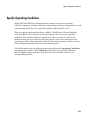
Specify Operating Conditions . . . . . . . . . . . . . . . . . . . .
5-21
Model Nonlinearity . . . . . . . . . . . . . . . . . . . . . . . . . . . . .
Amplifier and Mixer Nonlinearity Specifications . . . . .
Add Nonlinearity to Your System . . . . . . . . . . . . . . . .
5-23
5-23
5-24
Model Noise . . . . . . . . . . . . . . . . . . . . . . . . . . . . . . . . . . .
Amplifier and Mixer Noise Specifications . . . . . . . . . .
Add Noise to Your System . . . . . . . . . . . . . . . . . . . . .
Plot Noise . . . . . . . . . . . . . . . . . . . . . . . . . . . . . . . . . .
5-26
5-26
5-27
5-31
5-6
5-6
5-6
5-7
Plot Model Data
Create Plots . . . . . . . . . . . . . . . . . . . . . . . . . . . . . . . . . . . .
Available Data for Plotting . . . . . . . . . . . . . . . . . . . . . .
Validate Individual Blocks and Subsystems . . . . . . . . .
Types of Plots . . . . . . . . . . . . . . . . . . . . . . . . . . . . . . . .
Plot Formats . . . . . . . . . . . . . . . . . . . . . . . . . . . . . . . . .
How to Create a Plot . . . . . . . . . . . . . . . . . . . . . . . . . .
Example — Plot Component Data on a Z Smith Chart .
6-2
6-2
6-3
6-3
6-4
6-13
6-20
Update Plots . . . . . . . . . . . . . . . . . . . . . . . . . . . . . . . . . . .
6-25
Modify Plots . . . . . . . . . . . . . . . . . . . . . . . . . . . . . . . . . . .
6-26
Create and Modify Subsystem Plots . . . . . . . . . . . . . . .
Plot the Network Parameters of a Subsystem . . . . . . .
Add Data to an Existing Plot . . . . . . . . . . . . . . . . . . .
Change Data on an Existing Plot . . . . . . . . . . . . . . . .
6-28
6-28
6-30
6-32
vii
A
B
viii
Contents
SimRF Equivalent Baseband Algorithms
Simulate an RF Model . . . . . . . . . . . . . . . . . . . . . . . . . . .
A-2
Determine Modeling Frequencies . . . . . . . . . . . . . . . . . .
A-3
Map Network Parameters to Modeling Frequencies . .
A-5
Model Noise in an RF System . . . . . . . . . . . . . . . . . . . . .
Output-Referred Noise in RF Models . . . . . . . . . . . . . .
Calculate Noise Figure at Modeling Frequencies . . . . .
Calculate System Noise Figure . . . . . . . . . . . . . . . . . .
Calculate Output Noise Power . . . . . . . . . . . . . . . . . .
A-6
A-6
A-9
A-10
A-11
Create a Complex Baseband-Equivalent Model . . . . . .
Baseband-Equivalent Modeling . . . . . . . . . . . . . . . . . .
Simulation Efficiency of a Baseband-Equivalent Model
Example — Select Parameter Values for a BasebandEquivalent Model . . . . . . . . . . . . . . . . . . . . . . . . . .
A-12
A-12
A-16
Convert to and from Simulink Signals . . . . . . . . . . . . .
Signal Conversion Specifications . . . . . . . . . . . . . . . . .
Interpret Simulink Signals as Incident Power Waves .
Interpret Simulink Signals as Source Voltages . . . . . .
Specify Input Signal Conversions . . . . . . . . . . . . . . . .
A-31
A-31
A-32
A-34
A-35
A-17
Model Mixers
2-Port Mixer Blocks . . . . . . . . . . . . . . . . . . . . . . . . . . . . .
B-2
Model a Mixer Chain . . . . . . . . . . . . . . . . . . . . . . . . . . . .
B-4
Quadrature Mixers . . . . . . . . . . . . . . . . . . . . . . . . . . . . . .
Use SimRF Equivalent Baseband Software to Model
Quadrature Mixers . . . . . . . . . . . . . . . . . . . . . . . . . .
Model Upconversion I/Q Mixers . . . . . . . . . . . . . . . . . .
Model Downconversion I/Q Mixers . . . . . . . . . . . . . . . .
B-6
B-6
B-6
B-7
Simulate I/Q Mixers . . . . . . . . . . . . . . . . . . . . . . . . . . .
B-8
ix
Circuit Envelope
1
Sensitivity
• “Model System Noise Figure” on page 1-2
• “Designing a Receiver with an ADC” on page 1-8
1
Sensitivity
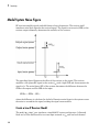
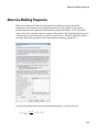
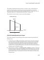
Model System Noise Figure
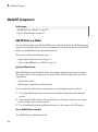
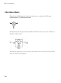
RF receivers amplify signals and shift them to lower frequencies. The receiver itself
introduces noise that degrades the received signal. The signal-to-noise ratio (SNR) at the
receiver output ultimately determines the usability of the receiver.
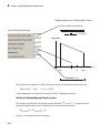
The preceding figure illustrates the effect of the receiver on the signal. The receiver
amplifies a low-power RF signal at the carrier fRF with a high SNR and downconverts the
signal to fIF. The noise figure (NF) of the system determines the difference between the
SNR at the output and the SNR at the input:
SNRout = SNRin − NFsys
where the difference is calculated in decibels. Excessive noise figure in the system causes
the noise to overwhelm the signal, making the signal unrecoverable.
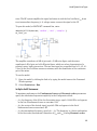
Create a Low-IF Receiver Model
The model ex_simrf_snr simulates a simplified IF receiver architecture. A Sinusoid
block and a Noise block model a two-tone input centered at fRF and low-level thermal
1-2
Model System Noise Figure
noise. The RF system amplifies the signal and mixes it with the local oscillator fLO down
to an intermediate frequency fIF. A voltage sensor recovers the signal at the IF.
To open this model, at MATLAB® command line, enter:
addpath(fullfile(docroot,'toolbox','simrf','examples'))
ex_simrf_snr
The amplifier contributes 40 dB of gain and a 15-dB noise figure, and the mixer
contributes 0 dB of gain and a 20-dB noise figure, which are values characteristic of a
relatively noisy, high-gain receiver. The two-tone input has a specified level of .1 μV. A 1V level in the local oscillator ensures consistency with the formulation of the conversion
gain of the mixer.
To run the model:
1
Open the model by clicking the link or by typing the model name at the Command
Window prompt.
2
Select Simulation > Run.
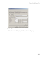
Set Up the SimRF Environment
To maximize performance, the Fundamental tones and Harmonic order parameters
specify the simulation frequencies explicitly in the Configuration block:
• fLO, the frequency of the LO in the first mixing stage, equals 1.9999 GHz. and appears
in the list of fundamental tones as carriers.LO.
• fRF, the carrier of the desired signal, equals 2 GHz and appears in the list of
fundamental tones as carriers.RF.
• fIF, the intermediate frequency, equals fRF – fLO. The frequency is a linear combination
of the first-order (fundamental) harmonics of fLO and fRF. Setting Harmonic order
1-3
1
Sensitivity
to 1 is sufficient to ensure this frequency appears in the simulation frequencies. This
minimal value for the harmonic order ensures a minimum of simulation frequencies.
Solver conditions and noise settings are also specified for the Configuration block:
• The Solver type is set to auto. For more information on choosing solvers, see the
reference page for the Configuration block or see Choosing Simulink® and Simscape™
Solvers.
• The Sample time parameter is set to 1/(mod_freq*64). This setting ensures a
simulation bandwidth 64 times greater than the envelope signals in the system.
• The Simulate noise box is checked, so the environment includes noise parameters
during simulation.
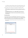
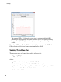
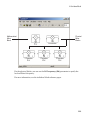
View Simulation Output
The model uses subsystems with a MATLAB Coder™ implementation of a fast Fourier
transform (FFT) to generate two plots. The FFT uses 64 bins, so for a sampling frequency
of 64 Hz, the bandwidth of each bin is 1 Hz. Subsequently, the power levels shown in the
figures also represent the power spectral density (PSD) of the signals in dBm/Hz.
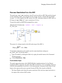
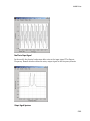
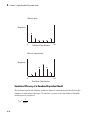
• The Input Display plot shows the power spectrum of the signal and noise at the input
of the receiver.
1-4
Model System Noise Figure
The measured power of each tone is consistent with the expected power level of a 0.1μV two-tone envelope:
 V2 
Pin = 10 log10 
 + 30
 2R 



−7 2
  1 ⋅ 10 
 2 2 


= 10 log10 
2
⋅
50







 + 30 = −142 dBm




A factor of 1/2 is due to voltage division across source and load resistors, and another
factor of 1/2 is due to envelope scaling. See the featured example Two-Tone Envelope
Analysis Using Real Signals for more discussion on scaling envelope signals for power
calculation.
The measured noise floor at -177 dBm/Hz is reduced by 3 dB from the specified
-174 dBm/Hz noise floor. The difference is due to power transfer from the source to the
input of the amplifier. The amplifier also models a thermal noise floor, so although
this decrease is unrealistic, it does not affect accuracy at the output stage.
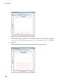
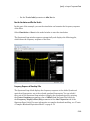
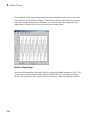
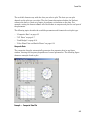
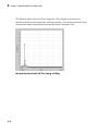
• The Output Display plot shows the power spectrum of the signal and noise at the
output of the receiver.
1-5
1
Sensitivity
The measured PSD of -102 dBm/Hz for each tone is consistent with the 40-dB
combined gain of the amplifier and mixer. The noise PSD in the figure is shown to
be approximately 50 dB higher at the output, due to the gain and noise figure of the
system.
If you have DSP System Toolbox™ software installed, you can replace the MATLAB
Coder subsystems with Vector Scope or Spectrum Analyzer blocks.
Simulating Thermal Noise Floor
Thermal noise power can be modeled according to the equation
Pnoise = 4 kBTRs∆f
where:
• kB is Boltzmann's constant, equal to 1.38065 × 10-23 J/K.
• T is the noise temperature, specified as 293.15 K in this example.
• Rs is the noise source impedance, specified as 50 Ω in this example to agree with the
resistance value of the Resistor block labeled R1.
• Δf is the noise bandwidth.
1-6
Model System Noise Figure
To model the noise floor on the RF signal at the resistor, the model includes a Noise
block:
• The Noise Power Spectral Density (Watts/Hz) parameter is calculated as
Pnoise / ∆f = 4 kBTRs .
• The Carrier frequencies parameter, set to carriers.RF, places noise on the RF
carrier only.
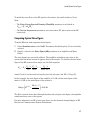
Computing System Noise Figure
To model RF noise from component noise figures:
1
Select Simulate noise in the SimRF Parameters block dialog box, if it is not already
selected.
2
Specify a value for the Noise figure (dB) parameter of an Amplifier and Mixer
blocks.
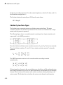
The noise figures are not strictly additive. The amplifier contributes more noise to the
system than the mixer because it appears first in the cascade. To calculate the total noise
figure of the RF system with n stages, use the Friis equation:
F - 1 F3 - 1
Fn - 1
Fsys = F1 + 2
+
+ ... +
G1
G1G2
G1G2 ...Gn -1
where Fi and Gi are the noise factor and gain of the ith stage, and NFi = 10log10(Fi).
In this example, the noise figure of the amplifier is 10 dB, and the noise figure of the
mixer is 15 dB, so the noise figure of the system is:
Ê
1015 /10 - 1 ˆ
10 log10 Á 1010 /10 +
˜ = 10.0 dB
Á
10000 ˜¯
Ë
The Friis equation shows that although the mixer has a higher noise figure, the amplifier
contributes more noise to the system.
For more information on RF system noise figure, see the featured example Impact of RF
Receiver on Communcations System Performance.
1-7
1
Sensitivity
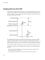
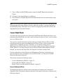
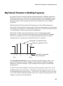
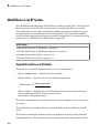
Designing a Receiver with an ADC
Most RF receivers in modern communications or radar systems feed signals to an analogto-digital converter (ADC). Due to their finite resolution, ADCs introduce quantization
error into the system. The resolution of the ADC is determined by the number of bits and
the full-scale (FS) range of the ADC.
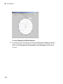
The preceding figure illustrates an RF signal that falls within the dynamic range (DR)
of an ADC. The input signal and noise at the carrier fRF has high signal-to-noise ratio
(SNR). The received signal at fIF has reduced SNR due to system noise figure. However, if
the quantization error is near or above the receiver noise, system performance degrades.
To ensure that the ADC contributes no more than 0.1 dB of noise to the signal at fIF, the
quantization noise floor must be 16 dB lower than the receiver noise. This condition can
be met by:
• Reducing the full-scale (FS) range or increasing the resolution of the ADC, which
lowers the quantization noise floor.
• Increasing the gain of the RF receiver, which raises the receiver noise floor.
1-8
Designing a Receiver with an ADC
Overcome Quantization Error of an ADC
The model ex_simrf_adc simulates a low-IF receiver with an ADC. This model is based
on the model ex_simrf_snr described in the section “Create a Low-IF Receiver Model”
on page 1-2. At the output of the RF system, the ADC subsystem models an ADC with an
FS range of sqrt(100e-3) V and a resolution of 16 bits.
To open this model, at MATLAB command line, enter:
addpath(fullfile(docroot,'toolbox','simrf','examples'))
ex_simrf_adc
The power of a voltage signal at the full-scale range of the ADC is
10 log10 100 −3 + 30 = 0 dBm
To maximize performance, the model uses the same simulation settings as
ex_simrf_snr. To run this model:
1
Open the model by clicking the link or by typing the model name at the Command
Window prompt.
2
Select Simulation > Run.
View Simulation Output
The model uses subsystems with a MATLAB Coder implementation of a fast Fourier
transform (FFT) to generate two plots. The FFT uses 64 bins, so for a sampling frequency
of 64 Hz, the bandwidth of each bin is 1 Hz. Subsequently, the power levels shown in the
figures also represent the power spectral density (PSD) of the signals in dBm/Hz.
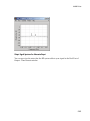
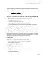
• The Input Display plot shows the power spectrum of the two-tone signal and noise at
the input of the receiver-ADC system.
1-9
1
Sensitivity
The measured power of each tone of -142 dBm is consistent with the expected power
level of a .1-μV signal. The power level of the noise is consistent with a -174 dBm/Hz
noise floor.
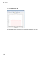
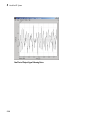
• The Output Display plot shows power spectrum of the output signal.
1-10
Designing a Receiver with an ADC
The quantization error exceeds the receiver noise.
If you have DSP System Toolbox software installed, you can replace the MATLAB Coder
subsystems with Vector Scope or Spectrum Analyzer blocks.
Measuring the Quantization Noise Floor
To calculate the quantization noise floor (QNF) of the ADC, subtract the dynamic range
from the full-scale power, which is 0 dBm. To calculate the dynamic range PSD for the
ADC, use the equation:
DRADC = 6.02 ⋅ N bits + 10 log10 ( ∆f ) + 1 .76 = 116 .1 dBm/Hz
where
• Nbits is the resolution. The ADC in this example uses 16 bits.
• Δf is the bandwidth of the FFT, which is 64 in this example. Oversampling in an ADC
yields lower quantization noise.
• The value 1.76 is a correction factor for a pure sinusoidal input.
Therefore, the quantization noise floor is -116 dBm/Hz, in agreement with the measured
output levels.
Improving Receiver-ADC Performance
Increasing the gain in the mixer raises the receiver noise without increasing the noise
figure. Calculate the mixer gain required to achieve a 16-dB margin between the
quantization noise floor and the receiver noise:
Gmixer = ( QNFADC + 16) - ( -174 + Gsys + NFsys)
= ( -116 .1 + 16) - ( -174 + 40 + 10 .0 )
= -100 .1 + 124.0
= 23 .9 dB
To simulate a receiver that clears the quantization noise floor:
1
Set the Available power gain parameter of the mixer to 23.9.
1-11
1
Sensitivity
2
Select Simulation > Run.
The figure shows that the receiver noise is 16 dB above the quantization noise floor.
1-12
2
Interference
• “Carrier to Interference Performance of a Weaver Receiver” on page 2-2
• “Model LO Phase Noise” on page 2-8
2
Interference
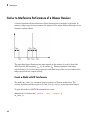
Carrier to Interference Performance of a Weaver Receiver
A classic superheterodyne architecture filters images prior to frequency conversion. In
contrast, image-reject receivers remove the images at the output without filtering but are
sensitive to phase offsets.
The preceding figure illustrates two input signals at the carriers fRF and fIM that both
differ from the LO frequency, fLO1, by an amount fIF1. Mixing translates both input
signals down to fIF1. Perfect image rejection in the final stage of the receiver removes the
image signal from the output entirely.
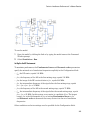
Create a Model with RF Interference
The model ex_simrf_ir simulates image rejection in a Weaver architecture. The
receiver downconverts the signals at fRF and fIM to fIF1 and fIF2 in two sequential stages.
To open this model, at MATLAB command line, enter:
addpath(fullfile(docroot,'toolbox','simrf','examples'))
ex_simrf_ir
2-2
Carrier to Interference Performance of a Weaver Receiver
To run the model:
1
Open the model by clicking the link or by typing the model name at the Command
Window prompt.
2
Select Simulation > Run.
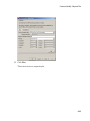
Set Up the SimRF Environment
To maximize performance, the Fundamental tones and Harmonic order parameters
specify the minimal set of simulation frequencies explicitly in the Configuration block:
• fRF, the RF carrier, equals 100 MHz.
• fLO1, the frequency of the LO in the first mixing stage, equals 150 MHz
• fIM, the image of the RF carrier relative to fLO1, equals 200 MHz.
• fIF1, the intermediate frequency of the signal after the first mixing stage, equals
fLO1 – fRF = fIM – fLO1 = 50 MHz.
• fLO2, the frequency of the LO in the second mixing stage, equals 75 MHz.
• fIF2, the intermediate frequency of the signal after the second mixing stage, equals
fLO2 – fIF1 = 25 MHz. In this system, every carrier is a multiple of fIF2. The largest
carrier, fIM, is the 8th harmonic of fIF2, so setting Fundamental tones to fIF2
and Harmonic order to 8 ensures that every carrier is in the set of simulation
frequencies.
Solver conditions and noise settings are also specified for the Configuration block:
2-3
2
Interference
• The Solver type is set to auto. For more information on choosing solvers, see the
reference page for the Configuration block or see Choosing Simulink and Simscape
Solvers.
• The Sample time parameter is set to 1/(mod_freq*64). This setting ensures a
simulation bandwidth 64 times greater than the envelope signals in the system.
• The Simulate noise box is checked, so the environment includes noise parameters
during simulation.
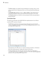
View Simulation Output
The model uses subsystems with a MATLAB Coder implementation of a fast Fourier
transform (FFT) to generate four plots.
• The RF Display plot shows the power spectrum of the signal recovered from the
carrier fRF, specified as carriers.RF in the Carrier frequencies parameter of the
preceding SimRF Outport block.
The modulation of the RF carrier is a constant envelope generated by a Continuous
Wave block which generates a single peak centered at the carrier.
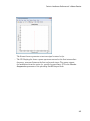
• The Image Display plot shows the power spectrum of the image. The signal is
recovered from the carrier fIM, specified as carriers.IM in the Carrier frequencies
parameter of the preceding SimRF Outport block.
2-4
Carrier to Interference Performance of a Weaver Receiver
The Sinusoid source generates a two-tone signal centered at fIM.
• The IF1 Display plot shows a power spectrum centered at the first intermediate
frequency, measured between the first and second stages. The sensor outputs
the modulation from the carrier fIF1, specified as carriers.IF2 in the Carrier
frequencies parameter of the preceding SimRF Outport block.
2-5
2
Interference
Both the RF and image appear on the carrier. The power level of the image 40 dB
higher than the RF.
• The Output Display plot shows the effects of the RF system. The sensor outputs
the modulation from the carrier fIF2, specified as carriers.IF1 in the Carrier
frequencies parameter of the preceding SimRF Outport block.
2-6
Carrier to Interference Performance of a Weaver Receiver
As expected, the system removes the image and amplifies the RF by 6 dB.
If you have DSP System Toolbox software installed, you can replace the MATLAB Coder
subsystems with Vector Scope or Spectrum Analyzer blocks.
Modeling RF and Blocker Sources
To model more robust input signals, you can use a SimRF Inport block to specify a
circuit envelope generated using blocks from other Simulink libraries. For example, the
featured example “Impact of an RF Receiver on Communication System Performance”
uses Communications System Toolbox™ blocks to model a QPSK-modulated waveform of
random bits with SimRF Inport that brings the signal into the SimRF environment.
Simulating LO Phase Offset
The phase shifters have specified Phase shift parameters of 90. Deviation from this
value results in a phase offset and causes imperfect image rejection. The featured
example “Measuring Image Rejection Ratio in Receivers” analyzes the IRR of the Weaver
and Hartley architectures several times, calculating the image rejection ratio (IRR) for
several different phase offsets.
2-7
2
Interference
Model LO Phase Noise
A mixer transfers local oscillator (LO) phase noise directly to its output.
The preceding figure shows the transfer of phase noise from fLO1 to fIF1.
Create a Model with Phase Noise
The model ex_simrf_phase_noise introduces phase noise into the model from the
section “Create a Model with RF Interference” on page 2-2. The first mixing stage
downconverts the RF and image to fIF
To open this model, at MATLAB command line, enter:
addpath(fullfile(docroot,'toolbox','simrf','examples'))
ex_simrf_phase_noise
2-8
Model LO Phase Noise
View Simulation Output
The model uses subsystems with a MATLAB Coder implementation of a fast Fourier
transform (FFT) to generate four plots.
• The IF1 Display plot shows a power spectrum centered at the first intermediate
frequency, measured between the first and second stages.
2-9
2
Interference
The figure shows that the LO phase noise has been transferred to the image. The RF
signal on the carrier fIF1 is not visible in the figure because its power level is below
the phase noise power of the downconverted image signal. The two visible peaks are
at the same power as the IF shown in the previous section, “Create a Model with RF
Interference” on page 2-2.
• The Output Display plot shows the downconverted RF with the images removed.
The LO phase noise has been transferred to the receiver output. The peak signal
power is the same as in the previous section, “Create a Model with RF Interference”
on page 2-2.
If you have DSP System Toolbox software installed, you can replace the MATLAB Coder
subsystems with Vector Scope or Spectrum Analyzer blocks.
Shaping the LO Noise Skirt
To simulate phase noise, the model phase modulates pink noise generated in the LO with
Phase Noise subsystem.
2-10
Model LO Phase Noise
The subsystem contains the following blocks:
• A Random Number block outputs a Gaussian random number at discrete time steps
to generate white noise.
• A Gain block scales the signal by a factor of
2p f LO1 10 Prel /10
where fLO1 is the LO frequency and Prel is the relative noise power density in dBc/Hz.
• A Discrete Filter block filters the uniform white noise to generate 1/f noise.
• A Magnitude-Angle to Complex block phase modulates an input signal ϕ. The output
is of the form exp(jϕ).
• An Inport block models a controlled voltage source in the SimRF environment,
modulating the carrier fLO with the input signal exp(jϕ). The circuit envelope
equivalent signal is exp[j(2πfLO1t + ϕ(t))].
If you have Communications System Toolbox software installed, use the Phase Noise
block to add phase noise to a given input signal.
2-11
3
Intermodulation Distortion
3
Intermodulation Distortion
Model a Direct Conversion Receiver
In this section...
“Create a Direct Conversion Receiver Model” on page 3-2
“Modeling IMD in System-Level Components” on page 3-6
“Examining DC Impairments” on page 3-7
Direct-conversion receivers are sensitive to second-order intermodulation products
because they transfer the RF signal directly to baseband.
Create a Direct Conversion Receiver Model
The model ex_simrf_dc models a direct-conversion receiver within the SimRF
environment. The RF system consists of a low-noise amplification (LNA) stage, a directconversion stage, and a final amplification stage.
To open this model, at MATLAB command line, enter:
addpath(fullfile(docroot,'toolbox','simrf','examples'))
ex_simrf_dc
To run the model:
3-2
1
Open the model by clicking the link or by typing the model name at the Command
Window prompt.
2
Select Simulation > Run.
Model a Direct Conversion Receiver
Set Up the SimRF Environment
The model runs according to the following environment settings:
• In the Configuration dialog box, the Fundamental tones parameter specifies the
carriers in the SimRF environment:
• fRF = fLO, the carrier of the RF and the local oscillator.
• fBL, the blocker carrier
The SimRF environment always simulates the 0 Hz carrier, regardless of whether the
SimRF Parameters block specifies it.
• In the Solver Configuration dialog box, the Use local solver box is selected. This
setting causes the SimRF environment to simulate with a local solver with the
following settings:
• Solver type is Trapezoidal rule.
• Sample time is sample_time, defined as 1.25e-4 in the model initialization
function.
Since the model uses a local solver, the global solver settings do not affect the
simulation within the SimRF environment. For more information on global and local
solvers, see Choosing Simulink and Simscape Solvers.
To maximize performance, the Fundamental tones and Harmonic order parameters
specify the simulation frequencies explicitly in the Configuration block:
• fRF = fLO, the carrier of the RF and the local oscillator, appears as a fundamental tone.
• fBL, the blocker carrier, appears as a fundamental tone.
• A carrier of 0 Hz, representing the passband signal, is included in the set of firstorder harmonics of both fundamental tones. Therefore, setting Harmonic order to
1 is sufficient to ensure this frequency appears in the simulation frequencies. This
minimal value for the harmonic order ensures a minimum of simulation frequencies.
Solver conditions and noise settings are also specified for the Configuration block:
• The Solver type is set to auto. For more information on choosing solvers, see the
reference page for the Configuration block or see Choosing Simulink and Simscape
Solvers.
3-3
3
Intermodulation Distortion
• The Sample time parameter is set to sample_time, which is equal to 1/
(mod_freq*64). This setting ensures a simulation bandwidth 64 times greater than
the envelope signals in the system.
• The Simulate noise box is checked, so the environment includes noise parameters
during simulation.
View Simulation Output
The model uses subsystems with a MATLAB Coder implementation of a fast Fourier
transform (FFT) to generate four plots:
• The RF Display plot shows the power level of the RF signal.
The power level of the RF is about 100 dBm.
• The Blocker Display plot shows the power spectrum centered at the carrier fBL..
3-4
Model a Direct Conversion Receiver
The power level of the blocker is about 90 dB higher than the signal power of the RF..
• The In-Phase Output plot shows the power spectrum of the in-phase signal at
baseband.
3-5
3
Intermodulation Distortion
In the figure, DC power is a direct result of the blocker and the IP2 in the mixers.
• The Quadrature Output plot shows the power spectrum of the quadrature signal at
baseband.
If you have DSP System Toolbox software installed, you can replace the MATLAB Coder
subsystems with Vector Scope or Spectrum Analyzer blocks.
Modeling IMD in System-Level Components
The IP2 and IP3 parameters specify the second- and third-order intercept points of
Amplifier and Mixer blocks:
• The amplifiers have infinite IP2 and IP3, so the amplifiers are linear.
• IP2 of the mixer is 15 dB
Amplifier and Mixer components have specified gains and noise figures:
• The gain and noise figure in the LNA stage are 25 dB and 6 dB, respectively.
• The gain and noise figure in the mixing stage are 10 dB and 10 dB. The Input
impedance (ohms) parameters of the two mixers are both 100, which sum in
parallel to a resistance of 50 Ω to match the output impedance of the LNA.
3-6
Model a Direct Conversion Receiver
• The gain and noise figure in the final amplification stage are 20 dB and 15 dB,
respectively.
To calculate RF system noise figure, use the Friis equation:
F - 1 F3 - 1
Fn - 1
Fsys = F1 + 2
+
+ ... +
G1
G1G2
G1G2 ...Gn -1
where Fi and Gi are the noise factor and gain of the ith stage. For more information
on RF system noise figure, see the featured example “Impact of an RF Receiver on
Communication System Performance”.
Examining DC Impairments
In addition to intermodulation distortion from IP2, direct-conversion receivers are subject
to additional DC impairments. For example, coupling between mixer input and local
oscillator (LO) ports causes self-mixing of the LO. For more information, see the featured
example “Executable Specification of a Direct Conversion Receiver”
3-7
SimRF Models
4
Analog Devices Transceiver Models
• “AD9361_TX Analog Devices Transmitter” on page 4-2
• “AD9361_RX Analog Devices Receiver” on page 4-4
4
Analog Devices Transceiver Models
AD9361_TX Analog Devices Transmitter
Model Overview
You can use the AD9361_TX model to simulate and verify Analog Devices AD9361 RF
transmitter designs. This model also helps to see the impact of RF imperfections on your
transmitted signal.
Install Analog Devices RF Transceivers using, simrfSupportPackages. You can open
the transmitter model using the Simulink Library Browser and opening SimRF Models
for Analog Devices RF Transceivers, or by typing the following in the MATLAB command
prompt:
ad9361_tx
Note: You require these additional licenses to run this model:
• Communications System Toolbox
• Fixed-Point Designer™
Complete documentation on how to use the models is available with the software
download.
Model Description
4-2
AD9361_TX Analog Devices Transmitter
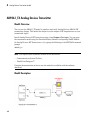
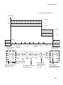
The transmitter model test bench consists of:
• Signal sources
• The AD9361 transmitter which is the device under test
• A spectrum analyzer
• A power meter
You can use the transmitter model to simulate the following behaviors:
• Tunable attenuation
• Oscillator phase noise
• Carrier–dependant noise floor
• Attenuation–and carrier–dependant non-linearities like output–referred third–order
intercept (OIP3)
• Attenuation–dependant gain imbalance
• Attenuation–dependant local oscillator (LO) carrier leak
4-3
4
Analog Devices Transceiver Models
AD9361_RX Analog Devices Receiver
Model Overview
You can use the AD9361_RX model to simulate and verify Analog Devices AD9361 RF
receiver designs. This model also helps to see the impact of RF imperfections on your
received signal.
Install Analog Devices RF Transceivers using, simrfSupportPackages. You can open
the receiver model using the Simulink library browser and opening SimRF Models for
Analog Devices RF Transceivers, or by typing the following in the MATLAB command
prompt:
ad9361_rx
Note: You require these additional licenses to run this model:
• Communications System Toolbox
• Stateflow®
• Fixed-Point Designer
Complete documentation on how to use the models is available with the software
download.
4-4
AD9361_RX Analog Devices Receiver
Model Description
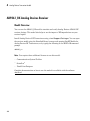
The receiver model test bench consists of:
• Signal sources
• The AD9361 receiver which is the device under test
• Analog filters
• Analog to Digital Convertor (ADC)
• Digital down-conversion filters (DDC)
• Receiver signal strength indicators
• Automatic gain control (AGC) state machine
• Gain table
You can use the receiver model to simulate the following behaviors:
• Tunable low–noise amplifier, mixer and trans–impedance amplifier (LMT) gains
• Carrier–dependent noise floor
• Gain–and carrier–dependant non-linearities like output–referred third–order
intercept (OIP3)
• Gain–and carrier–dependant non-linearities like output–referred second–order
intercept (OIP2)
• Gain–dependant gain imbalance
4-5
4
Analog Devices Transceiver Models
• Gain–dependant local oscillator (LO) carrier leak
4-6
Equivalent Baseband
5
Model an RF System
• “Model RF Components” on page 5-2
• “Specify or Import Component Data” on page 5-6
• “Specify Operating Conditions” on page 5-21
• “Model Nonlinearity” on page 5-23
• “Model Noise” on page 5-26
5
Model an RF System
Model RF Components
In this section...
“Add RF Blocks to a Model” on page 5-2
“Connect Model Blocks” on page 5-3
Add RF Blocks to a Model
You can include blocks from the SimRF Equivalent Baseband Physical and Mathematical
libraries in a Simulink model. For more information on the libraries and the available RF
blocks, see “SimRF Equivalent Baseband Libraries”.
This section contains the following topics:
• “Input Signal Requirements” on page 5-2
• “How to Add RF Blocks to a Model” on page 5-2
Input Signal Requirements
Most SimRF Equivalent Baseband blocks only support complex single-channel signals.
The signals can be either sample-based or frame-based. The following blocks have this
requirement:
• All Physical blocks
• Mathematical Amplifier and Mixer blocks
You can model the effect of these components on a multichannel signal as follows:
1
Use a Simulink Demux block to split the multichannel signal into single-channel
signals.
2
Create duplicate RF models, with one model for each channel, and pass each singlechannel signal into a separate model.
3
Use a Simulink Mux block multiplex the signals at the output of the RF models.
How to Add RF Blocks to a Model
To add RF blocks to a Simulink model:
5-2
Model RF Components
1
Type rflib at the MATLAB prompt to open the SimRF Equivalent Baseband
library.
2
Navigate to the desired library or sublibrary.
3
Drag instances of SimRF Equivalent Baseband blocks into the model window using
the mouse.
Note: You can also access SimRF Equivalent Baseband blocks and other Simulink blocks
from the Simulink Library Browser window. Open this window by typing simulink at
the MATLAB prompt. Add blocks to the model by dragging them from this window and
dropping them into the model window.
Connect Model Blocks
You follow the same procedure for connecting SimRF Equivalent Baseband blocks as for
connecting Simulink blocks: you click a port and drag the mouse to draw a line to another
port on a different block.
You can only connect blocks that use the same type of signal. Physical library blocks
use different types of signals than Mathematical library blocks, and are represented
graphically by a different port style. Therefore, you can freely connect pairs of
Mathematical modeling blocks. You can also freely connect pairs of Physical modeling
blocks. However, you cannot directly connect Physical blocks to Mathematical blocks.
Instead, you must use the Input Port and Output Port blocks to bridge them.
For more information on the Physical and Mathematical libraries, including how to
open the libraries and a description of the available blocks, see “Overview of SimRF
Equivalent Baseband Libraries”.
This section contains the following topics:
• “Connect Mathematical Blocks” on page 5-3
• “Connect Physical Blocks” on page 5-4
• “Bridge Physical and Mathematical Blocks” on page 5-4
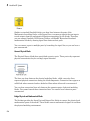
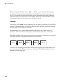
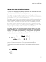
Connect Mathematical Blocks
The Mathematical library blocks use the same input and output ports as standard
Simulink blocks. These ports show the direction of the signal at the port, as shown in the
following diagram.
5-3
5
Model an RF System
Similar to standard Simulink blocks, you draw lines between the ports of the
Mathematical modeling blocks, called signal lines, to represent signals that are inputs
to and outputs from the mathematical functions represented by the blocks. Therefore,
you can connect Simulink, DSP System Toolbox, and SimRF Equivalent Baseband
mathematical blocks by drawing signal lines between their ports.
You can connect a port to multiple ports by branching the signal line, or you can leave a
port unconnected.
Connect Physical Blocks
The Physical library blocks have specialized connector ports. These ports only represent
physical connections; they do not imply signal direction.
The lines you draw between the physical modeling blocks, called connection lines,
represent physical connections among the block components. Connection lines appear as
solid black when connected and as dashed red lines when either end is unconnected.
You can draw connection lines only between the connector ports of physical modeling
blocks. You cannot branch these connection lines. You cannot leave connector ports
unconnected.
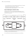
Bridge Physical and Mathematical Blocks
The blockset provides the Input Port and Output Port blocks to connect the physical and
mathematical parts of the model. These blocks convert mathematical signals to and from
the physical modeling environment.
5-4
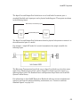
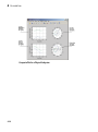
Model RF Components
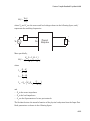
The Input Port and Output Port blocks have one of each kind of connector port: a
standard Simulink style input port and a physical modeling port. These ports are shown
in the following figure:
Mathematical, or Simulink style, ports
Physical Modeling Ports
The Input Port and Output Port blocks must bound a physical subsystem to connect it to
the mathematical part of a model.
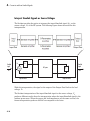
For example, a simple RF model of a coaxial transmission line might resemble the
following figure.
The Microstrip Transmission Line block uses an Input Port block to get its white noise
input from a Random Source block, and an Output Port block to pass its output to a
Spectrum Scope block. The Random Source and Spectrum Scope blocks are from DSP
System Toolbox library.
For information on how SimRF Equivalent Baseband software converts mathematical
signals to and from the physical modeling environment, see “Convert to and from
Simulink Signals” on page A-31.
5-5
5
Model an RF System
Specify or Import Component Data
In this section...
“Specify Parameter Values” on page 5-6
“Supported File Types for Importing Data” on page 5-6
“Import Data Files into RF Blocks” on page 5-7
“Example — Import a Touchstone Data File into an RF Model” on page 5-10
“Import Circuits from the MATLAB Workspace” on page 5-13
“Example — Import a Bandstop Filter into an RF Model” on page 5-14
Specify Parameter Values
There are two ways to set block parameter values:
• Using the GUI — Enter information in the block dialog boxes, which open when you
double-click a block in the Simulink window.
• Using commands — Use the Simulink set_param and get_param commands to set
and get parameter values of the blocks, respectively. For more information on these
commands, see the set_param and get_param reference pages.
Supported File Types for Importing Data
The blockset also lets you import the following types of data files:
• Industry-standard file formats — Touchstone S2P, Y2P, Z2P, and H2P formats specify
the network parameters and noise information for measured and simulated data.
For more information on Touchstone files, see http://www.vhdl.org/pub/ibis/connector/
touchstone_spec11.pdf.
• Agilent® P2D file format — Specifies amplifier and mixer large-signal, powerdependent network parameters, noise data, and intermodulation tables for several
operating conditions, such as temperature and bias values.
The P2D file format lets you import system-level verification models of amplifiers and
mixers.
5-6
Specify or Import Component Data
• Agilent S2D file format — Specifies amplifier and mixer network parameters with
gain compression, power-dependent S21 parameters, noise data, and intermodulation
tables for several operating conditions.
The S2D file format lets you import system-level verification models of amplifiers and
mixers.
• MathWorks™ amplifier (AMP) file format — Specifies amplifier network parameters,
power data, noise data, and third-order intercept point
For more information about .amp files, see “AMP File Format” in the RF Toolbox™
documentation.
• MATLAB circuits — RF Toolbox circuit objects in the MATLAB workspace specify
network parameters, noise data, and third-order intercept point information of
circuits with different topologies.
For more information about RF circuit objects, see “RF Circuit Objects” in the RF
Toolbox documentation.
Import Data Files into RF Blocks
The blockset lets you import industry-standard data files, Agilent P2D and S2D files,
and MathWorks AMP files into specific blocks to simulate the behavior of measured
components in the Simulink modeling environment.
This section contains the following topics:
• “Blocks Used to Import Data” on page 5-7
• “How to Import Data Files” on page 5-8
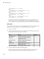
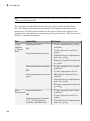
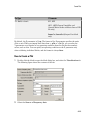
Blocks Used to Import Data
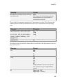
Three blocks in the Physical library accept data from a file. The following table lists the
blocks and any corresponding data format that each supports.
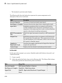
Block
Description
Supported Format(s)
General Amplifier
Generic amplifier
Touchstone, AMP, P2D, S2D
General Mixer
Generic mixer
Touchstone, AMP, P2D, S2D
General Passive Network
Generic passive component
Touchstone
5-7
5
Model an RF System
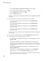
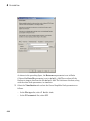
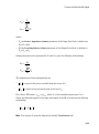
How to Import Data Files
To import a data file:
1
Choose the block that best represents your component from the list of blocks that
accept file data shown in “Blocks Used to Import Data” on page 5-7.
2
Open the Physical library, and navigate to the sublibrary that contains the block.
3
Click and drag the block into your Simulink model.
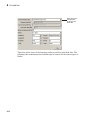
4
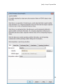
In the block dialog box, enter the name of your data file for the Data file parameter.
The file name must include the extension. If the file is not in your MATLAB path,
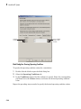
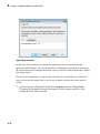
specify the full path to the file or use the Browse button to find the file.
Note: The Data file parameter is only enabled when the Data source parameter is
set to Data file. This is the default setting and it means the block data comes from
a file.
5-8
Specify or Import Component Data
5-9
5
Model an RF System
The following section shows an example of this procedure.
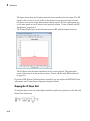
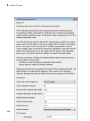
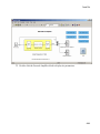
Example — Import a Touchstone Data File into an RF Model
In this example, you model the frequency response of a passive component using data
from a Touchstone file, defaultbandpass.s2p.
You use a model from one of the SimRF Equivalent Baseband examples to perform the
following tasks:
• “Import Data into a General Passive Network Block” on page 5-10
• “Validate the Passive Component” on page 5-12
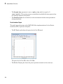
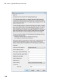
Import Data into a General Passive Network Block
In this part of the example, you inspect the defaultbandpass.s2p file and import data
into the RF model using the General Passive Network block.
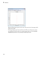
1
Type the following at the MATLAB prompt to open the defaultbandpass.s2p file:
edit defaultbandpass.s2p
The following figure shows a portion of the .s2p file.
5-10
Specify or Import Component Data
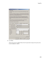
The option line
# GHz S RI R 50
specifies the following information about the contents of the data file:
• GHz — Frequency units.
• S — Network parameters are S-parameters.
• RI — Network parameters are specified as the real and imaginary parts.
• R 50 — Reference impedance is 50 ohms.
For more information about the Touchstone specification, including the option line,
see http://www.vhdl.org/pub/ibis/connector/touchstone_spec11.pdf.
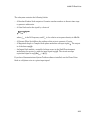
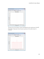
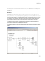
2
At the MATLAB prompt, type
sparam_filter
5-11
5
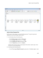
Model an RF System
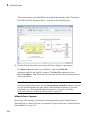
This command opens the SimRF Equivalent Baseband example called “Touchstone
Data File for 2-Port Bandpass Filter,” as shown in the following figure.
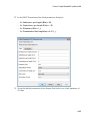
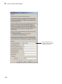
3
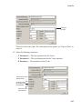
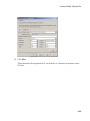
Double-click the General Passive Network block to display its parameters.
The Data source parameter is set to Data file, so the Data file
parameter specifies the data file to import. The Data file parameter is set to
defaultbandpass.s2p. The block uses this data with the other block parameters
during simulation.
Note: When the imported file contains data that is measured at frequencies other
than the modeling frequencies, use the Interpolation method parameter to specify
how the block determines the data values at the modeling frequencies. For more
information, see “Determine Modeling Frequencies” on page A-3 and “Map
Network Parameters to Modeling Frequencies” on page A-5.
Validate the Passive Component
In this part of the example, you plot the network parameters of the General Passive
Network block to validate the data you imported in “Import Data into a General Passive
Network Block” on page 5-10.
5-12
Specify or Import Component Data
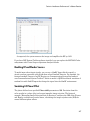
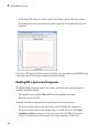
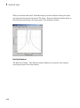
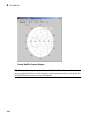
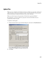
1
Open the General Passive Network block dialog box, and select the Visualization
tab.
2
Set the Source of frequency data parameter to User-specified.
3
Set the Frequency data (Hz) parameter to [0.5e9:0.1e6:1.5e9].
4
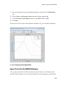
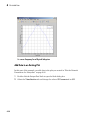
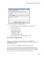
Click Plot.
These actions create a plot of the magnitude and phase of S21 as a function of frequency.
S21 versus Frequency for the Imported Data
Import Circuits from the MATLAB Workspace
You can only connect Physical library blocks in cascade. However, the blockset works
with RF Toolbox software to let you include additional circuit topologies in an RF model.
5-13
5
Model an RF System
To model circuit topologies that contain other types of connections, you must define a
circuit in the MATLAB workspace and import it into an RF model.
To import a circuit from the MATLAB workspace:
1
Define the circuit object in the MATLAB workspace using the RF Toolbox functions.
For more information about RF circuit objects, see the RF Toolbox documentation for
“RF Circuit Objects”.
2
Add a General Circuit Element block to your RF model from the Black Box Elements
sublibrary of the Physical library. For information on how to open this library, see
“Open SimRF Equivalent Baseband Libraries”.
3
Enter the circuit object name in the RFCKT object parameter in the General
Circuit Element block dialog box.
This procedure is illustrated by example in the following section.
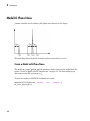
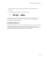
Example — Import a Bandstop Filter into an RF Model
In this example, you simulate the frequency response of a filter that you model using
circuit objects from the MATLAB workspace.
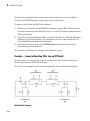
The filter in this example is the 50-ohm bandstop filter shown in the following figure.
Bandstop Filter Diagram
5-14
Specify or Import Component Data
You represent the filter using four circuit objects that correspond to the four parts of the
filter, ckt1, ckt2, ckt3, and ckt4 in the diagram. You use an input signal with random,
complex input values that have a Gaussian distribution to stimulate the filter. The scope
block displays the output signal.
This example illustrates how to perform the following tasks:
• “Create Circuit Objects in the MATLAB Workspace” on page 5-15
• “Build the Model” on page 5-16
• “Specify and Import Component Data” on page 5-17
• “Run the Simulation and Plot the Results” on page 5-19
Create Circuit Objects in the MATLAB Workspace
In this part of the example, you define MATLAB variables to represent the physical
properties of the filter shown in the previous figure, Bandstop Filter Diagram, and use
functions from RF Toolbox software to create RF circuit objects that model the filter
components.
1
Type the following at the MATLAB prompt to define the filter's capacitance and
inductance values in the MATLAB workspace:
C1
C2
C3
C4
C5
C6
L1
L2
L3
L4
L5
L6
2
=
=
=
=
=
=
=
=
=
=
=
=
1.734e-12;
4.394e-12;
7.079e-12;
7.532e-12;
1.734e-12;
4.394e-12;
25.70e-9;
3.760e-9;
17.97e-9;
3.775e-9;
17.63e-9;
25.70e-9;
Type the following at the MATLAB prompt to create RF circuit objects that model
the components labeled ckt1, ckt2, ckt3, and ckt4 in the circuit diagram:
ckt1 = ...
rfckt.series('Ckts',{rfckt.shuntrlc('C',C1),...
5-15
5
Model an RF System
rfckt.shuntrlc('L',L1,'C',C2)});
ckt2 = ...
rfckt.parallel('Ckts',{rfckt.seriesrlc('L',L2),...
rfckt.seriesrlc('L',L3,'C',C3)});
ckt3 = ...
rfckt.parallel('Ckts',{rfckt.seriesrlc('L',L4),...
rfckt.seriesrlc('L',L5,'C',C4)});
ckt4 = ...
rfckt.series('Ckts',{rfckt.shuntrlc('C',C5),...
rfckt.shuntrlc('L',L6,'C',C6)});
For more information about the RF Toolbox objects used in this example, see the
rfckt.series class, rfckt.parallel class, rfckt.shuntrlc class, and
rfckt.seriesrlc class object reference pages in the RF Toolbox documentation.
Build the Model
In this portion of the example, you create a Simulink model. For more information about
adding and connecting components, see “Model RF Components” on page 5-2.
1
Create a new model.
2
Add to the model the blocks shown in the following table. The Library column of the
table specifies the hierarchical path to each block.
3
Block
Library
Quantity
Random Source
DSP System Toolbox > Sources
1
Input Port
SimRF > Equivalent Baseband >
Input/Output Ports
1
General Circuit
Element
SimRF > Equivalent Baseband >
Black Box Elements
4
Output Port
SimRF > Equivalent Baseband >
Input/Output Ports
1
Spectrum Analyzer
DSP System Toolbox > Sinks
1
Connect the blocks as shown in the following figure.
Change the names of your General Circuit Element blocks to match those in the
figure by double-clicking the text below the block and typing a new name.
5-16
Specify or Import Component Data
Specify and Import Component Data
In this portion of the example, you specify block parameters. To open the parameter
dialog box for each block, double-click the block.
1
In the Random Source block dialog box:
• Set the Source type parameter to Gaussian.
• Set the Sample time parameter to 1/100e6.
• Set the Samples per frame parameter to 256.
• Set the Complexity parameter to Complex.
Selecting these settings creates an input signal with random, complex input values
that have a Gaussian distribution.
2
In the Input Port block dialog box:
• Set the Treat input Simulink signal as parameter to Incident power wave.
5-17
5
Model an RF System
• Set the Finite impulse response filter length parameter to 256.
• Set the Center frequency (Hz) parameter to 400e6.
• Set the Sample time parameter to 1/100e6.
• Clear the Add noise check box.
Selecting these settings defines the physical characteristics and modeling bandwidth
of the filter.
3
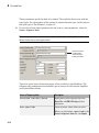
Set the parameters of the General Circuit Element blocks as follows:
• In the General Circuit Element1 block dialog box, set the RFCKT object
parameter to ckt1.
• In the General Circuit Element2 block dialog box, set the RFCKT object
parameter to ckt2.
• In the General Circuit Element3 block dialog box, set the RFCKT object
parameter to ckt3.
• In the General Circuit Element4 block dialog box, set the RFCKT object
parameter to ckt4.
Selecting these settings imports the circuit objects that model the filter components
into the model.
4
In the Output Port block dialog box, set the Load impedance parameter to 50.
5
Set the Spectrum Analyzer block parameters as follows:
• In the View tab, under Spectrum Settings , set the Averages under Trace
options to 100.
This parameter establishes the number of spectra that the scope averages to
produce the displayed signal. You use a value of 100 because the input signal is
random and you want to display the average filter response over a large number
of input values.
• In the View tab, under Spectrum Settings , set the Units under Trace
options to dBm/Hertz.
• In the View tab, under Configuration Properties, set the Minimum Ylimit parameter to -75 and the Maximum Y-limit parameter to -45.
These values set the range of x- and y-values on the display such that the entire
signal is visible when you run the simulation.
5-18
Specify or Import Component Data
• Set the Y-axis label parameter to dBm/Hertz.
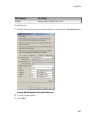
Run the Simulation and Plot the Results
In this part of the example, you run the simulation and examine the frequency response
of the filter.
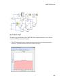
Select Simulation > Start in the model window to start the simulation.
The Spectrum Scope window appears automatically and displays the following plot,
which shows the frequency response of the filter.
Frequency Response of Bandstop Filter
The Spectrum Scope block displays the frequency response at the shifted (basebandequivalent) frequencies, not at the selected passband frequencies. You can relabel
the x-axis of the Spectrum Scope window to display the passband signal by entering
the Center frequency parameter value of 400e6 (from the Input Port block) for
the Frequency display offset (Hz) parameter in the Axis Properties tab of the
Spectrum Scope block. For more information on complex-baseband modeling, see “Create
a Complex Baseband-Equivalent Model” on page A-12.
5-19
5
Model an RF System
References
Geffe, P.R., “Novel designs for elliptic bandstop filters,” RF Design, February 1999.
5-20
Specify Operating Conditions
Specify Operating Conditions
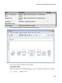
Agilent P2D and S2D files contain simulation results at one or more operating
conditions. Operating conditions define the independent parameter settings that are used
when creating the file data. The specified conditions differ from file to file.
When you import component data from a .p2d or .s2d file into a General Amplifier
or General Mixer block, the block contains parameter values for several operating
conditions. The available conditions depend on the data in the file. By default, the
blockset defines the object behavior using the property values that correspond to the
operating conditions that appear first in the file. To use other property values, you must
select a different operating condition in the block dialog box.
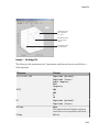
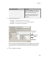
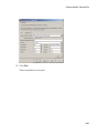
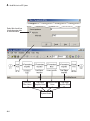
If the block contains data at multiple operating conditions, the Operating Conditions
tab contains two columns. The Conditions column shows the available conditions,
and the Values column contains a drop-down list of the available values for the
corresponding condition.
5-21
5
Model an RF System
Available
conditions
Lists of available
values for each
condition
Block Dialog Box Showing Operating Conditions
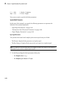
To specify the operating condition values for a simulation:
1
Double-click the block to open the block dialog box.
2
Select the Operating Conditions tab.
3
In the Conditions column, find the condition to specify. Select the corresponding
pull-down list in the Values column, and choose the desired operating condition
value.
Repeat the preceding step as needed to specify the desired operating condition values.
5-22
Model Nonlinearity
Model Nonlinearity
In this section...
“Amplifier and Mixer Nonlinearity Specifications” on page 5-23
“Add Nonlinearity to Your System” on page 5-24
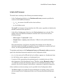
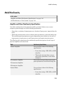
Amplifier and Mixer Nonlinearity Specifications
You define nonlinearity for the physical amplifier and mixer blocks at one or more
frequency points through one of the following specifications:
• Power data, consisting of output power as a function of input power, imported into the
block.
• Third-order intercept data, with or without power parameters, in the block dialog box.
The available power parameters are gain compression power (defined as the ratio of
output power to input power at small input power) and output saturation power.
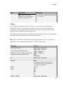
The following table summarizes the nonlinearity specification options for each type of
physical amplifier and mixer block.
Block
Nonlinearity Specification
General Amplifier
You can choose either of the following
specifications:
• Power data (using a P2D, S2D, or AMP
data file)
• Third-order intercept data or one or
more power parameters, in the block
dialog box.
S-Parameters Amplifier
Y-Parameters Amplifier
Third-order intercept data or one or more
power parameters, in the block dialog box.
Z-Parameters Amplifier
General Mixer
You can choose either of the following
specifications:
• Power data (using a P2D, S2D, or AMP
data file)
5-23
5
Model an RF System
Block
Nonlinearity Specification
• Third-order intercept data or one or
more power parameters, in the block
dialog box.
S-Parameters Mixer
Third-order intercept data or one or more
power parameters, in the block dialog box.
Y-Parameters Mixer
Z-Parameters Mixer
Add Nonlinearity to Your System
To simulate the nonlinearity of an amplifier or mixer, you must specify or import
nonlinearity data at one or more frequency points into the block.
The method you use to add nonlinearity data to a block depends on whether you specify
the data manually or import the data into a block.
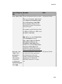
The following table provides instructions for adding nonlinearity data.
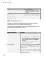
Nonlinearity Specification
Instructions
IP3
In the Nonlinearity Data tab of the block dialog
box:
• Set the IP3 type parameter to IIP3 or OIP3.
• Enter input third-order intercept values at one
or more frequency points in the IP3 (dBm)
parameter.
• Enter corresponding frequency values in the
Frequency (Hz) parameter.
Power parameters
Enter the gain compression power in the 1 dB gain
compression power (dBm) parameter or the
saturation power in the Output saturation power
(dBm) parameter.
If you choose a scalar value for the Frequency (Hz)
parameter, then you must also use scalar values for
the power parameters.
5-24
Model Nonlinearity
Nonlinearity Specification
Instructions
If you choose a vector value for the Frequency (Hz)
parameter, then you can use either scalar or vector
values for the power parameters.
Power data (from a file)
Import file data that includes power information
into the Data file or RFCKT object parameter of
the General Amplifier or General Mixer block.
Note: If you import file data with no power information into a General Amplifier
or General Mixer block, the Nonlinearity Data tab lets you add nonlinearity data
manually in the block dialog box.
For information on how the blockset simulates nonlinearity data of an amplifier or mixer,
see the block reference page.
5-25
5
Model an RF System
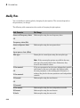
Model Noise
In this section...
“Amplifier and Mixer Noise Specifications” on page 5-26
“Add Noise to Your System” on page 5-27
“Plot Noise” on page 5-31
Amplifier and Mixer Noise Specifications
You only need to specify noise information for the physical amplifier and mixer blocks
that generate noise other than resistor noise. For the other blocks, the blockset calculates
the noise automatically based on the resistor values.
You define noise for the physical amplifier and mixer blocks through one of the following
specifications:
• Spot noise data in the data source.
• Spot noise data in the block dialog box.
• Spot noise data (rfdata.noise class) object in the block dialog box.
• Frequency-independent noise figure, noise factor, or noise temperature value in the
block dialog box.
• Frequency-dependent noise figure data (rfdata.nf) object in the block dialog box.
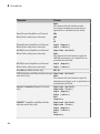
The following table summarizes the noise specification options for each type of physical
amplifier and mixer block.
Block
Noise Specification
General Amplifier
Spot noise data (using a Touchstone, P2D,
S2D, or AMP data file)
OR
Spot noise data, noise figure value, noise
factor value, noise temperature value,
rfdata.noise, or rfdata.nf object in
the block dialog box
5-26
Model Noise
Block
Noise Specification
S-Parameters Amplifier
Spot noise data, noise figure value, noise
factor value, noise temperature value,
rfdata.noise, or rfdata.nf object in
the block dialog box
Y-Parameters Amplifier
Z-Parameters Amplifier
General Mixer
Spot noise data (using a Touchstone, P2D,
S2D, or AMP data file)
OR
Spot noise data, noise figure value, noise
factor value, noise temperature value,
rfdata.noise, or rfdata.nf object in
the block dialog box
S-Parameters Mixer
Y-Parameters Mixer
Z-Parameters Mixer
Spot noise data, noise figure value, noise
factor value, noise temperature value,
rfdata.noise, or rfdata.nf object in
the block dialog box
Add Noise to Your System
To simulate the noise of a physical subsystem, you perform the following tasks:
• “Specify or Import Noise Data” on page 5-27
• “Add Noise to the Simulation” on page 5-29
Specify or Import Noise Data
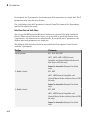
The method you use to add noise data to a block depends on whether you are specifying
noise data manually or importing spot-noise data.
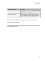
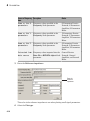
The following table provides instructions for adding noise data.
Noise Specification
Instructions
Frequency-independent noise figure
In the Noise Data tab of the block dialog
box, set the Noise type parameter to
Noise figure, and enter the noise figure
value in the Noise figure (dB) parameter.
5-27
5
Model an RF System
Noise Specification
Instructions
Frequency-dependent noise figure
In the Noise Data tab of the block dialog
box, set the Noise type parameter to
Noise figure, and enter the name of
the rfdata.nf object in the Noise figure
(dB) parameter.
Noise factor
In the Noise Data tab of the block dialog
box, set the Noise type parameter to
Noise factor, and enter the noise factor
value in the Noise factor parameter.
Noise temperature
In the Noise Data tab of the block dialog
box, set the Noise type parameter to
Noise temperature, and enter the
noise temperature value in the Noise
temperature (K) parameter.
Spot noise data (in a block dialog box)
In the Noise Data tab of the block dialog
box, set the Noise type parameter to
Spot noise data. Enter the spot noise
information in the Minimum noise figure
(dB), Optimal reflection coefficient,
and Equivalent normalized noise
resistance parameters.
Spot noise data (from a data object)
In the Noise Data tab of the block dialog
box, set the Noise type parameter to
Noise figure and enter the name of the
rfdata.noise object in the Noise figure
(dB) parameter.
Spot noise data (from a file)
Import file data that includes noise
information into the Data file or RFCKT
object parameter of the General Amplifier
or General Mixer block.
Note: If you import file data with no noise information into a General Amplifier or
General Mixer block, the Noise Data tab lets you add noise data manually in the block
dialog box.
5-28
Model Noise
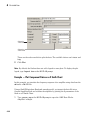
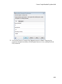
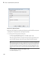
Add Noise to the Simulation
To include noise in the simulation, you must select the Add noise check box on the Input
Port block dialog box. This check box is selected by default.
5-29
5
Model an RF System
5-30
Model Noise
For information on how the blockset simulates noise, see “Model Noise in an RF System”
on page A-6.
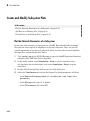
Plot Noise
SimRF Equivalent Baseband software models communications systems. The noise in
these systems has a very small amplitude, typically from 1e-6 to 1e-12 Watts. In contrast,
the default signal power of a Communications System Toolbox modulator block is 1 Watt
at a nominal 1 ohm. Therefore, the signal-to-noise ratio in an RF system simulation is
large, making it difficult to view the noise that the RF system adds to your signal.
To display the noise on a plot, you might need to attenuate the signal amplitude to a
value within a couple orders of magnitude of the noise.
For example, suppose you have the following model that contains a multitone test signal
source.
5-31
5
Model an RF System
When you simulate this model, Simulink brings up several windows showing the input
and output for the physical subsystem. The Input - Frequency Domain window shown in
the following figure displays the input signal in the frequency domain.
Input Signal Spectrum
The Real Part of Input - Time Domain window displays the real part of the complexvalued input signal in the time domain.
5-32
Model Noise
Real Part of Input Signal
In the model, the physical subsystem adds noise to the input signal. The Output Frequency Domain window shows the noisy output signal in the frequency domain.
Output Signal Spectrum
5-33
5
Model an RF System
The amplitude of the signal is large compared to the amplitude of the noise, so the noise
is not visible in the Real Part of Output - Time Domain window that shows the real part
of the time-domain output signal. Therefore, you must attenuate the amplitude of the
input signal to display the noise of the time-domain output signal.
Real Part of Output Signal
Attenuate the amplitude of the input signal by setting the Gain parameter to 1e-3. This
is equivalent to attenuating the input signal by 60 dB. When you run the model again,
the two signal peaks are not as pronounced in the Output - Frequency Domain window.
5-34
Model Noise
Output Signal Spectrum for Attenuated Input
You can now view the noise that the RF system adds to your signal in the Real Part of
Output - Time Domain window.
5-35
5
Model an RF System
Real Part of Output Signal Showing Noise
5-36
6
Plot Model Data
• “Create Plots” on page 6-2
• “Update Plots” on page 6-25
• “Modify Plots” on page 6-26
• “Create and Modify Subsystem Plots” on page 6-28
6
Plot Model Data
Create Plots
In this section...
“Available Data for Plotting” on page 6-2
“Validate Individual Blocks and Subsystems” on page 6-3
“Types of Plots” on page 6-3
“Plot Formats” on page 6-4
“How to Create a Plot” on page 6-13
“Example — Plot Component Data on a Z Smith Chart” on page 6-20
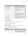
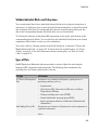
Available Data for Plotting
SimRF Equivalent Baseband software lets you validate the behavior of individual RF
components and physical subsystems in your model by plotting the following data:
• Large- and small-signal S-parameters
• Noise figure, noise factor and noise temperature
• Output third-order intercept point
• Power data
• Phase noise
• Voltage standing-wave ratio
• Transfer function
• Group delay
• Reflection coefficients
Note: When you plot information about a physical block, the blockset plots the actual
frequency response of the block, as specified in the block dialog box. The blockset does not
plot the frequency response of the complex-baseband model that it uses to simulate the
block, in which the frequency response is centered at zero. For more information on how
the blockset simulates physical blocks, see Appendix A.
6-2
Create Plots
Validate Individual Blocks and Subsystems
You can plot model data for an individual physical block or for a physical subsystem. A
subsystem is a collection of one or more physical blocks bracketed by an Input Port block
and an Output Port block. To understand the behavior of specific subsystems, plot the
data of the corresponding Output Port block after you run a simulation.
To validate the behavior of individual RF components in the model, plot the data of the
corresponding physical blocks. You can plot data for individual blocks from each of these
components either before or after you run a simulation.
You create a plot by selecting options in the block dialog box, as shown in “Create and
Modify Subsystem Plots” on page 6-28. To learn about the available plots, see “Types
of Plots” on page 6-3. For more information about creating plots, see “How to Create
a Plot” on page 6-13.
Types of Plots
SimRF Equivalent Baseband software provides a variety of plots for analyzing the
behavior of RF components and subsystems. The following table summarizes the
available plots and charts and describes each one.
Plot Type
Plot Contents
X-Y Plane (Rectangular)
Plot
Parameters as a function of frequency, input power, or
operating condition, such as
• S-parameters
• Noise figure (NF), Noise factor (NFactor), and Noise
Temperature (NTemp)
• Voltage standing-wave ratio (VSWR)
• Output third-order intercept point (OIP3)
• Input and output reflection coefficients (GammaIn and
GammaOut)
Link Budget Plot (3-D)
Parameters as a function of frequency for each component in
a physical subsystem
where
6-3
6
Plot Model Data
Plot Type
Plot Contents
The curve for a given component represents the cumulative
contribution of each RF component up to and including the
parameter value of that component.
For more information, see “Link Budget” on page 6-10.
Polar Plane Plot
Magnitude and phase of parameters as a function of
frequency or operating condition, such as
• S-parameters
• Input and output reflection coefficients (GammaIn and
GammaOut)
Smith® Chart
Real and imaginary parts of S-parameters as a function of
frequency or operating condition, used for analyzing the
reflections caused by impedance mismatch.
Composite Plot
Multiple plots and charts in one figure.
To learn how to create these plots, see “How to Create a Plot” on page 6-13.
Plot Formats
When you create a plot from a block dialog box, you must specify the format of the data
for both the x- and y-axes.
These plot options define how SimRF Equivalent Baseband software displays the data on
the plot.
6-4
Create Plots
The available formats vary with the data you select to plot. The data you can plot
depends on the plot type you select. The plot formats determine whether the blockset
converts the data to a new set of units, or performs a calculation on the data. For
example, setting the format to Real tells the blockset to compute and plot the real part of
the parameter.
The following topics describe the available parameters and formats for each plot type:
• “Composite Data” on page 6-5
• “X-Y Plane” on page 6-7
• “Link Budget” on page 6-10
• “Polar Plane Plots and Smith Charts” on page 6-12
Composite Data
The composite data plot automatically generates four separate plots in one figure
window, showing the frequency dependence of several parameters. The following figure
shows an example of such a plot.
Example — Composite Data Plot
6-5
6
Plot Model Data
Note: For composite data plots, you do not need to specify the parameters or the formats
—they are set automatically.
The combination of plots differs based on the type of block and the specified block
data. The following table describes the contents of the composite data plot for each
specification. The Plot Contents column lists the types of plots as they appear on the
composite plot, counterclockwise and starting in the upper-left corner. The blockset plots
all data as a function of frequency.
Block
Specified Data
Plot Contents
General
Amplifier
or General
Mixer
Network parameters
• X-Y plot, magnitude of S12 and S21
in decibels
OR
Network parameters and noise
• X-Y plot, phase of S12 and S21 in
degrees
• Z Smith Chart, real and imaginary
parts of S11 and S22
• Polar plot, magnitude and phase of
S11 and S22
Network parameters and power
OR
Network parameters, noise, and
power
• X-Y plot, magnitude of S12 and S21
in decibels
• X-Y plot, output power (Pout) in
dBm (decibels referenced to one
milliwatt)
• Z Smith Chart, real and imaginary
parts of S11 and S22
• Polar plot, magnitude and phase of
S11 and S22
Other
Network parameters
Physical block
OR
Network parameters and noise
(S-, Y-, and Z-Parameters
Amplifiers and Mixers only)
6-6
• X-Y plot, magnitude of S12 and S21
in decibels
• X-Y plot, phase of S12 and S21 in
degrees
• Z Smith Chart, real and imaginary
parts of S11 and S22
Create Plots
Block
Specified Data
Plot Contents
• Polar plot, magnitude and phase of
S11 and S22
Note: Only the General
Amplifier and General Mixer
blocks accept power data.
X-Y Plane
You can plot any parameters that are relevant to your block on an X-Y plane plot.
For this type of plot, you specify data for both the x- and y-axes. If you specify two Y
parameters, and you specify different formats for the two Y parameters, the blockset
plots the second Y parameter on the right y-axis.
The following table summarizes the available Y parameters and formats. The parameters
and formats are the same for both the left and right y-axes.
Note: LS11, LS12, LS21, and LS22 are large-signal S-parameters. You can plot these
parameters as a function of input power or as a function of frequency.
Y Parameter
Y Format
S11, S12, S21, S22
LS11, LS12, LS21, LS22 (General
Amplifier and General Mixer blocks with
multiple operating conditions only)
Magnitude (decibels)
Magnitude (linear)
Angle (degrees)
Angle (radians)
Real
Imaginary
NF
Magnitude (decibels)
NFactor
None
This format tells the blockset to plot
the noise factor as it is specified to or
calculated by the block.
NTemp
Kelvin
OIP3
dBm
dBW
W
mW
VSWRIn, VSWROut
Magnitude (decibels)
6-7
6
Plot Model Data
Y Parameter
Y Format
None
This format tells the blockset to plot
the voltage standing-wave ratio as it is
specified to or calculated by the block.
Pout (General Amplifier and General
Mixer blocks with power data only)
dBm
dBW
W
mW
Phase (General Amplifier and General
Mixer blocks with power data only)
Angle (degrees)
Angle (radians)
AM/AM (General Amplifier and General
Mixer blocks with power data only)
Magnitude (decibels)
None
This format tells the blockset to plot the
AM/AM conversion as it is specified to or
calculated by the block.
AM/PM (General Amplifier and General
Mixer blocks with power data only)
Angle (degrees)
Angle (radians)
PhaseNoise (Mixer blocks only)
dBc/Hz
FMIN (Amplifier and Mixer blocks with spot Magnitude (decibels)
noise data only)
None
This format tells the blockset to plot the
minimum noise figure as it is specified to or
calculated by the block.
6-8
GammaIn, GammaOut(Output Port block
only)
Magnitude (decibels)
Magnitude (linear)
Angle (degrees)
Angle (radians)
Real
Imaginary
GAMMAOPT (Amplifier and Mixer blocks
with spot noise data only)
Magnitude (decibels)
Magnitude (linear)
Angle (degrees)
Angle (radians)
Real
Imaginary
Create Plots
Y Parameter
Y Format
RN (Amplifier and Mixer blocks with spot
noise data only)
None
This format tells the blockset to plot the
noise resistance as it is specified to or
calculated by the block.
The available X parameters depend on the Y parameters you select. The following table
summarizes the available X parameters for each of the Y parameters in the preceding
table.
Y Parameter
X Parameter
Pout, Phase, LS11, LS12, LS21, LS22
Pin
Freq
S11, S12, S21, S22, NF, OIP3, VSWRIn,
VSWROut, GAMMAIn, GAMMAOut, FMIN,
GAMMAOPT, RN
Freq
AM/AM, AM/PM
AM
The following table shows the X formats that are available for the X parameters listed in
the preceding table.
X Parameter
X Format
Pin
dBm
dBW
W
mW
Freq
THz
GHz
MHz
KHz
Hz
Auto (xformat is chosen to provide the
best scaling for the given xparameter
values.)
AM
Magnitude (dB)
Magnitude (linear)
6-9
6
Plot Model Data
When you import block data from a .p2d or .s2d file, you can also plot Y parameters
as a function of any operating condition from the file that has numeric values, such as
bias. You can specify an operating condition as the X parameter only when validating
individual blocks, and the format is always None. This format tells the blockset to plot
the operating condition values as they are specified in the file.
Link Budget
You use the Link budget plot to understand the individual contribution of each block to
a plotted Y parameter value in a physical subsystem with multiple components between
the Input Port and the Output Port blocks.
The link budget plot is a three-dimensional plot that shows one or more curves of
parameter values as a function of frequency, ordered by the subsystem circuit index.
The following figure shows how the circuit index is assigned to a component in a physical
subsystem based on its sequential position in the subsystem.
Input Port
Component
(Index = 1)
Component
(Index = 2)
...
Component
(Index = n)
Output Port
A curve on the link budget plot for each circuit index represents the contributions to the
parameter value of the RF components up to that index. The following figure shows an
example of a link budget plot.
6-10
Create Plots
Contributions to S21
from components
1, 2, and 3
Contributions to S21
from components
1 and 2
Contributions to S21
from component 1
Example — Link Budget Plot
The following table summarizes the Y parameters and formats that are available for a
link budget plot.
Y Parameter
Y Format
S11, S12, S21, S22
Magnitude (decibels)
Magnitude (linear)
Angle (degrees)
Real
Imaginary
OIP3
dBm
dBW
W
mW
NF
Magnitude (decibels)
Magnitude (linear)
NFactor
None
This format tells the blockset to plot the
noise factor as it is specified to the block.
NTemp
Kelvin
6-11
6
Plot Model Data
If you specify two Y parameters, the blockset puts both parameters in a single plot. The Y
parameters must have the same formats.
For a link budget plot, the X parameter is always Freq. The format of the X parameter
specifies the units of the x-axis.
Polar Plane Plots and Smith Charts
You can use SimRF Equivalent Baseband software to generate Polar plots and Smith
Charts. When you select these plot types, you do not need to specify the format of any
Y parameters—the formats are set automatically. If you specify two Y parameters, the
blockset puts both parameters in a single plot.
The following table describes the Polar plot and Smith Chart options. It also lists the
available Y parameters.
Plot Type
Y Parameter
Polar plane
S11, S12, S21, S22
LS11, LS12, LS21, LS22 (General
Amplifier and General Mixer blocks with
data from a P2D file only)
GammaIn, GammaOut (Output Port block
only)
Z Smith chart
S11, S22
LS11, LS22 (General Amplifier and
General Mixer blocks with data from a P2D
file only)
GammaIn, GammaOut (Output Port block
only)
Y Smith chart
S11, S22
LS11, LS22 (General Amplifier and
General Mixer blocks with data from a P2D
file only)
GammaIn, GammaOut (Output Port block
only)
6-12
Create Plots
Plot Type
Y Parameter
ZY Smith chart
S11, S22
LS11, LS22 (General Amplifier and
General Mixer blocks with data from a P2D
file only)
GammaIn, GammaOut (Output Port block
only)
By default, the X parameter is Freq. The format of the X parameter specifies the units
of the x-axis. When you import block data from a .p2d or .s2d file, you can also plot
Y parameters as a function of any operating condition from the file that has numeric
values, such as bias. You can specify an operating condition as the X parameter only
when validating individual blocks, and the format is always None.
How to Create a Plot
1
Double-click the block to open the block dialog box, and select the Visualization tab.
The following figure shows the contents of the tab.
2
Select the Source of frequency data.
6-13
6
Plot Model Data
Select the source
of frequencies
at which to plot
block data
This value is the source of the frequency values at which to plot block data. The
following table summarizes the available types of sources for the various types of
blocks.
6-14
Create Plots
Source of frequency Description
data
User-specified
Blocks
Vector of frequencies that you enter. All physical blocks
When you select User-specified
in the Source of frequency data
list, the Frequency range (Hz)
field is displayed. Enter a vector
specifying the range of frequencies
you want to plot.
For example, to plot block data from
0.3 MHz to 5 GHz by 0.1 MHz, enter
[0.3e6:0.1e6:5e9].
Note: When you select PhaseNoise
in the Parameter list and
User-specified in the Source
of frequency data list, the
Frequency range (Hz) field is
disabled. You use the Phase noise
frequency offset (Hz) block
parameter to specify the frequency
values at which to plot block data.
Derived from
Input Port
parameters
(Available
after running
a simulation
or clicking the
Update Diagram
button
Modeling frequencies derived from
the Input Port block parameters.
For information on how the
blockset computes the modeling
frequencies, see “Determine
Modeling Frequencies” on page
A-3.
All physical blocks
)
6-15
6
Plot Model Data
Source of frequency Description
data
3
Blocks
Same as the Sparameters
Frequency values specified in the
Frequency block parameter.
S-Parameters Passive
Network, S-Parameters
Amplifier, S-Parameters
Mixer
Same as the Yparameters
Frequency values specified in the
Frequency block parameter.
Y-Parameters Passive
Network, Y-Parameters
Amplifier, Y-Parameters
Mixer
Same as the Zparameters
Frequency values specified in the
Frequency block parameter.
Z-Parameters Passive
Network, Z-Parameters
Amplifier, Z-Parameters
Mixer
Extracted from
data source
Frequency values imported into the
Data file or RFDATA object block
parameter.
General Passive
Network, General
Amplifier, and General
Mixer
Enter the Reference impedance.
Enter the
reference
impedance
This value is the reference impedance to use when plotting small-signal parameters.
4
6-16
Select the Plot type.
Create Plots
Select the
plot type
This value is the type of plot. For a description of the options, see “Types of Plots” on
page 6-3.
5
Select the following parameters:
• Y Parameter1 — The first parameter for the Y-axis.
• Y Parameter2 — The second parameter for the Y-axis (optional).
• X Parameter — The parameter for the X-axis.
Select the first Y-axis
plot parameter
Optionally, select
the second Y-axis
plot parameter
Select the X-axis
plot parameter
6-17
6
Plot Model Data
These parameters specify the data to be plotted. The available choices vary with the
type of plot. For a description of the options for a particular plot type, see the topic on
that plot type in “Plot Formats” on page 6-4.
6
If you select a large-signal parameter for one or more y-axis parameters, select the
Source of power data.
Note: Large-signal parameters are available only for General Amplifier or General
Mixer blocks that contain power data.
Select the source
of input power
values at which
to plot block data
This value is the source of the input power values at which to plot block data. The
following table summarizes the available types of sources for the General Amplifier
and General Mixer blocks.
Source of frequency data
Description
Extracted from data source
Input power values imported into the
Data file or RFDATA object block
parameter.
User-specified
Vector of power values that you enter.
When you select User-specified in the
Source of power data list, the Input
6-18
Create Plots
Source of frequency data
Description
power data (dBm) field is displayed.
Enter a vector specifying the range of
power values you want to plot.
For example, to plot block data from
1 dBm to 10 dBm by 2 dBm, enter
[1:2:10].
7
Select the following formats:
• Y Format1 — The format for the first Y parameter.
• Y Format2 — The format for the second Y parameter (optional).
• X Format — The format for the X parameter.
Select the format
for Y parameter1
Optionally, select
the format for
Y parameter2
Select the format
for X parameter
These are the X and Y formats for plotting the selected parameter. The available
choices vary based on the selected parameter. For a description of the options for
a particular plot type, see the topic on that plot type in “Plot Formats” on page
6-4.
8
Select the X Scale and Y Scale.
6-19
6
Plot Model Data
Select the
Y-axis scale
Select the
X-axis scale
These are the scales on which to plot the data. The available choices are Linear and
Log.
9
Click Plot.
Note: By default, the blockset does not add a legend to some plots. To display the plot
legend, type legend show at the MATLAB prompt.
Example — Plot Component Data on a Z Smith Chart
In this example, you simulate the frequency response of an amplifier using data from the
default.s2d S2D file.
Using a SimRF Equivalent Baseband example model, you import the data file into a
General Amplifier block and validate the amplifier by plotting the S-parameters of the
block on a Z Smith Chart.
1
6-20
Type sparam_amp at the MATLAB prompt to open the “AMP Data File for
Amplifier” example.
Create Plots
2
Double-click the General Amplifier block to display its parameters.
6-21
6
Plot Model Data
As shown in the preceding figure, the Data source parameter is set to Data
fileand the Data file parameter is set to default.s2d. These values tell the
blockset to import data from the file default.s2d. The block uses this data, along
with the other block parameters, in simulation.
3
Select the Visualization tab and set the General Amplifier block parameters as
follows:
• In the Plot type list, select Z Smith chart.
• In the Y Parameter1 list, select S22.
6-22
Create Plots
4
Click Plot.
This action creates a Z Smith Chart of the S22 parameters using the frequency data
from the default.s2d file.
6-23
6
Plot Model Data
General Amplifier Frequency Response
Note: To display data tips for a plotted line, select Tools > Data Cursor. Click the data
cursor on the plotted line to see the frequency and the parameter value at that point. See
the MATLAB documentation for more information.
6-24
Update Plots
Update Plots
When you run a simulation, the blockset continues to display any open plots, but does not
update the plots to reflect new simulation results. You must update the subsystem plots
after the simulation to display the behavior of the revised subsystem.
When you make changes to the parameters of blocks that represent individual
RF components, you need to update any open plots, because the blockset does not
automatically redraw the plots.
To update an existing plot:
1
Double-click the block to open the block dialog box, and select the Visualization tab.
Example Block Dialog Box Showing Visualization Tab
2
Click Plot.
6-25
6
Plot Model Data
Modify Plots
You can modify an existing plot by changing the plot options. The outcome depends on
the parameter you change.
The following table summarizes the results of changing the plot options.
Block Parameter
Plot Change
Source of frequency data
Redraws plot using the new frequency data.
OR
Frequency data (Hz)
Source of power data
Redraws plot using the new power data.
OR
Input power data (dBm)
Plot type
Draws plot in a new figure using the new plot type.
Note: If the current plot options are valid for the new
plot type, they retain their values. Otherwise, they
revert to their default values.
Y Parameter2
If the new parameter has the same independent variable
and format as the one on the plot, the blockset adds
the new parameter to the existing plot. Otherwise, it
redraws the plot for the new parameter and independent
variable.
Y Format1
Redraws plot using the new format.
Y Parameter1
OR
OR
Y Format2
6-26
X Parameter
Redraws plot using the new independent variable.
X Format
Redraws plot using the new format.
X Scale
Redraws plot using the new scale.
Modify Plots
Block Parameter
Plot Change
Y Scale
Redraws plot using the new scale.
To modify a plot:
1
Double-click the block to open the block dialog box, and select the Visualization tab.
Example Block Dialog Box Showing Plot Parameters
2
Change the plot options.
3
Click Plot.
6-27
6
Plot Model Data
Create and Modify Subsystem Plots
In this section...
“Plot the Network Parameters of a Subsystem” on page 6-28
“Add Data to an Existing Plot” on page 6-30
“Change Data on an Existing Plot” on page 6-32
Plot the Network Parameters of a Subsystem
In this part of the example, you open and run a SimRF Equivalent Baseband example
that uses file data to specify an amplifier in a physical subsystem. Then, you plot the
network parameters of the physical subsystem, which consists of the General Amplifier,
the Input Port, and the Output Port blocks.
1
Type sparam_amp at the MATLAB prompt to open the SimRF Equivalent Baseband
example called “AMP Data File for Amplifier”.
2
In the model window, select Simulation > Start to run the simulation. Once
the simulation has reached steady state, select Simulation > Stop to stop the
simulation.
3
Double-click the Output Port block to open the block dialog box.
4
Select the Visualization tab and set the Output Port block parameters as follows:
• In the Source of frequency data list, select Derived from Input Port
parameters.
• In the Plot type list, select X-Y plane.
• In the Y Parameter1 list, select S21.
6-28
Create and Modify Subsystem Plots
5
Click Plot.
This action plots the magnitude of S21 (in decibels) as a function of frequency on an
X-Y plot.
6-29
6
Plot Model Data
S21 versus Frequency for a Physical Subsystem
Add Data to an Existing Plot
In this part of the example, you add data to the plot you created in “Plot the Network
Parameters of a Subsystem” on page 6-28.
6-30
1
Double-click the Output Port block to open the block dialog box.
2
Select the Visualization tab and change the value of Y Parameter1 to S22.
Create and Modify Subsystem Plots
3
Click Plot.
This action adds S22 to the plot.
6-31
6
Plot Model Data
S21 and S22 versus Frequency for a Physical Subsystem
Change Data on an Existing Plot
In this part of the example, you change the data on the plot you created in the previous
steps of the example by modifying the Plot type.
1
Double-click the Output Port block to open the block dialog box.
2
Select the Visualization tab and change the value of Plot type to Polar plane, as
shown in the following figure.
As the figure shows, the value of Y Parameter1 remains as S22, the last parameter
selected for the previous plot.
6-32
Create and Modify Subsystem Plots
3
Click Plot.
This action creates a Polar plane plot of S22 as a function of frequency.
6-33
6
Plot Model Data
S22 versus Frequency for a Physical Subsystem
4
6-34
In the Output Port block dialog box, change the Plot type to Composite data to
generate four plots in one figure. The parameters for the plots are defined by the
block, so the Y Parameter1, Y Parameter2, and X Parameter fields becomes
invisible.
Create and Modify Subsystem Plots
5
Click Plot.
This action creates a composite plot.
6-35
6
Plot Model Data
Composite Plot for a Physical Subsystem
6-36
A
SimRF Equivalent Baseband Algorithms
A
Simulate an RF Model
Simulate an RF Model
When you simulate a model that contains physical blocks, SimRF Equivalent Baseband
software determines the modeling frequencies of the physical system using the Input
Port block parameters. The modeling frequencies are the frequencies at which the
blockset takes information from the blocks to construct the baseband-equivalent model.
Then, the software determines the block parameter values at those frequencies and
uses the information to create a baseband-equivalent model for Simulink time-domain
simulation.
A-2
Determine Modeling Frequencies
Determine Modeling Frequencies
When you simulate an RF model, the Output Port block uses Input Port block
parameters to determine the modeling frequencies f for the physical system that is
bracketed between the Input Port block and the Output Port block. f is an N-element
vector, where N is the finite impulse response filter length. The modeling frequencies are
a function of the center frequency fc and the sample time ts. The following figure shows
the Input Port block parameters that determine the modeling frequencies.
fn is the nth element of the vector of modeling frequencies, f, and is given by
fn = f min +
n -1
n = 1,..., N
ts N
A-3
A
Determine Modeling Frequencies
where
fmin = f c -
A-4
1
2ts
Map Network Parameters to Modeling Frequencies
Map Network Parameters to Modeling Frequencies
In a physical system, each block provides network parameters at different frequencies.
These frequencies are not necessarily the modeling frequencies for the physical system
in which the block resides. To create a baseband-equivalent model, SimRF Equivalent
Baseband software must calculate the values of the S-parameters at the modeling
frequencies.
Individual physical blocks calculate the S-parameters at the modeling frequencies
determined by the Input Port block parameters. Each block interpolates its S-parameters
to determine the S-parameters at the modeling frequencies. If the block contains network
Y- or Z-parameters, it first converts them to S-parameters.
Specifically, the block orders the S-parameters in the ascending order of their
frequencies, fn. Then, it interpolates the S-parameters using the MATLAB interp1
function. For example, the curve in the following diagram illustrates the result of
interpolating the S11 parameters at original frequencies f1 through f5.
Interpolated S11 parameter values
Original S11 parameter values
f1
(fmin)
f2
f4
f5
f3
Frequencies in ascending
order of magnitude
(fmax)
The Interpolation method field in the individual block dialog boxes enables you to
specify the interpolation method as Cubic, Linear (default), or Spline. For more
information about these methods, see the interp1 reference page in the MATLAB
documentation.
As shown in the previous diagram, each block uses the parameter values at fmin for all
modeling frequencies smaller than fmin. The block uses the parameter values at fmax for
all modeling frequencies greater than fmax. In both cases, the results may not be accurate,
so you need to specify network parameter values over a range of frequencies that is wide
enough to account for the block behavior.
A-5
A
Model Noise in an RF System
Model Noise in an RF System
The SimRF Equivalent Baseband Physical library blocks can model noise. The Input Port
block parameters specify whether to include noise in a simulation. When you include
noise information in your model, the blockset simulates the noise of the physical system
by combining the noise contributions from each individual block. This section explains
how the blockset simulates noise from user-specified information. For information on how
to add noise to an RF model, see “Model Noise” on page 5-26.
In this section...
“Output-Referred Noise in RF Models” on page A-6
“Calculate Noise Figure at Modeling Frequencies” on page A-9
“Calculate System Noise Figure” on page A-10
“Calculate Output Noise Power” on page A-11
Output-Referred Noise in RF Models
In general, you can specify output-referred noise in one of three ways:
• Noise temperature — Specifies the noise in kelvin.
• Noise factor — Specifies the noise by the following equation:
Noise factor = 1 +
Noise temperature
290
• Noise figure — Specifies the noise in decibels relative to the standard reference
noise temperature of 290 K. In terms of noise factor
Noise figure = 10log(Noise factor)
These three specifications are equivalent, because you can compute each one from any of
the others.
The blockset lets you simulate the noise associated with any physical block in your RF
model.
The blockset automatically determines the noise properties of passive blocks from their
network parameters. The blockset gets these network parameters either explicitly from
A-6
Model Noise in an RF System
the block dialog box or specified data files, or implicitly by calculating them from the
specified block parameters.
For active devices such as amplifiers and mixers, the noise properties can not be inferred
from network parameters. Therefore, for the amplifier and mixer blocks, you must specify
the noise information explicitly, either in the dialog block or the associated data file.
For physical amplifier and mixer blocks, you can specify active block noise in one of the
following ways:
• Spot noise data
• Frequency-independent noise figure, noise factor, or noise temperature values
• Frequency-dependent noise figure data (rfdata.nf) or spot noise data
(rfdata.noise) object
These noise specification options are described in “Amplifier and Mixer Noise
Specifications” on page 5-26.
When you run the simulation, the blockset first computes the noise figure values for each
individual block at the modeling frequencies. Then, it computes the noise figure of the
physical system from the individual noise figure values and uses the system noise figure
information to calculate the output noise power. This process is shown in the following
figure.
A-7
A
Model Noise in an RF System
Select this check box
to include noise data
in the simuliation
Front-End
Filter Noise
Final Stage
Low-Noise
Downconverter
Amplifier Noise
Amplifier Noise
Noise
System Noise
A-8
Model Noise in an RF System
Calculate Noise Figure at Modeling Frequencies
To include noise information in a simulation, the blockset must compute the noise figure
values of each individual block at the modeling frequencies.
If you specify the frequency-independent noise figure value directly, or if the blockset
computes the noise figure value from the block resistance, the blockset uses this value for
the noise figure value at each of the modeling frequencies.
If you specify the noise factor or noise temperature value, the blockset computes the noise
figure value from the specified value using the equations in the preceding section and
uses the computed value for the noise figure value at each of the modeling frequencies.
If you specify frequency-dependent noise figure values using an rfdata.nf object, the
blockset interpolates the values using the Interpolation method specified in the block
dialog box to get the noise figure value at each of the modeling frequencies.
If you specify spot noise data, the blockset computes frequency-dependent noise figure
information from this data. It takes the minimum noise figure, NFmin, equivalent noise
resistance, Rn, and optimal source admittance, Yopt, values in the file and interpolates
to find the values at the modeling frequencies. Then, the blockset uses the following
equation to calculate the noise correlation matrix, CA:
CA
È
Rn
Í
= 2 kT Í
Í NFmin - 1
- Rn Yopt
ÍÎ
2
NFmin - 1
˘
- Rn Yopt* ˙
2
˙
2
˙
Rn Yopt
˙˚
where k is Boltzmann's constant, and T is the noise temperature in Kelvin.
The blockset then calculates the noise factor, F, from the noise correlation matrix as
follows:
F =1+
z+ CA z
2kT Re {ZS }
È 1 ˘
z = Í *˙
ÍÎ ZS ˙˚
A-9
A
Model Noise in an RF System
In the two preceding equations, ZS is the nominal impedance, which is 50 ohms, and z+ is
the Hermitian conjugation of z.
The blockset obtains the noise figure, NF, from the noise factor:
NF = 10 log( F)
Calculate System Noise Figure
The blockset uses a recursive process to calculate system noise figure. The noise
correlation matrices for the first two elements of the cascade are combined into a single
matrix, and the process is repeated.
The following figure shows a cascaded network consisting of two 2-port networks, each
represented by its ABCD-parameters.
First, the blockset calculates noise correlation matrices CA' and CA” for the two networks.
Then, the blockset combines CA′ and CA″ into a single correlation matrix CA using the
equation
 A′ B′  ″  A′
CA = C′A + 
 CA 
 C′ D′ 
 C′
B′ 

D′
The ABCD-parameter matrices in the cascade combine according to matrix
multiplication:
A

C
B  A′
 =
D  C′
B′   A″

D′  C″
B″ 

D″ 
If there is another element in the cascade, the same calculations will be performed using
these ABCD-parameters as well as the ABCD-parameters corresponding to the following
element. The recursion will terminate with a noise correlation matrix pertaining to the
entire system. The blockset then calculates the system noise figure from this matrix.
A-10
Model Noise in an RF System
For more information about these calculation techniques, see the following article:
Hillbrand, H. and P.H. Russer, “An Efficient Method for Computer Aided Noise Analysis
of Linear Amplifier Networks,” IEEE Transactions on Circuits and Systems, Vol. CAS-23,
Number 4, pp. 235–238, 1976.
Calculate Output Noise Power
The blockset uses noise power to determine the amplitude of the noise that it adds to the
physical system using a Gaussian distributed pseudorandom number generator. It uses
both the noise temperature and the modeling bandwidth to calculate the noise power:
Noise power = kTB
where k is Boltzmann's constant, T is the noise temperature in Kelvin, and B is the
bandwidth in hertz.
The blockset computes noise temperature from the specified or calculated noise figure
values for the system, and it computes the modeling bandwidth from the model's sample
time and center frequency.
A-11
A
Create a Complex Baseband-Equivalent Model
Create a Complex Baseband-Equivalent Model
In this section...
“Baseband-Equivalent Modeling” on page A-12
“Simulation Efficiency of a Baseband-Equivalent Model” on page A-16
“Example — Select Parameter Values for a Baseband-Equivalent Model” on page
A-17
Baseband-Equivalent Modeling
SimRF Equivalent Baseband software simulates the physical system in the time domain
using a complex baseband-equivalent model that it creates from the passband frequencydomain parameters of the physical blocks. This type of modeling is also known as
lowpass equivalent (LPE), complex envelope, or envelope modeling.
To create a complex baseband-equivalent model in the time domain based on the network
parameters of the physical system, the blockset performs a mathematical transformation
that consists of the following three steps:
1
“Calculate the Passband Transfer Function” on page A-12
2
“Calculate the Baseband-Equivalent Transfer Function” on page A-14
3
“Calculate the Baseband-Equivalent Impulse Response” on page A-15
Calculate the Passband Transfer Function
The blockset calculates the passband transfer function from the physical block
parameters at the modeling frequencies by calculating the transfer function of the
physical subsystem and then applying the Tukey window to obtain the passband transfer
function.
Note: To learn how the blockset uses the specified network parameters to compute the
network parameters at the modeling frequencies, see “Map Network Parameters to
Modeling Frequencies” on page A-5.
The transfer function of the physical subsystem is defined as:
A-12
Create a Complex Baseband-Equivalent Model
H( f ) =
VL ( f )
VS ( f )
where VS and VL are the source and load voltages shown in the following figure, and f
represents the modeling frequencies.
Zs
+
+
Vin
-
Vs
-
+
Physical
Subsystem
Z
L
VL
-
More specifically,
H( f ) =
S21 (1 + Γ l ) ( 1 − Γ s )
2 ( 1 − S22 Γl ) (1 − Γin Γ s )
where
Zl − Zo
Zl + Zo
Z − Zo
Γs = s
Zs + Zo
Γl =


Γl
Γ in = S11 +  S12 S21


(1 − S22Γ l ) 

and
• ZS is the source impedance.
• ZL is the load impedance.
• Sij are the S-parameters of a two-port network.
The blockset derives the transfer function of the physical subsystem from the Input Port
block parameters as shown in the following figure.
A-13
A
Create a Complex Baseband-Equivalent Model
Passband Spectrum of a Modulated RF Carrier
N is the number of sub-bands
Input Port Block Parameters
Df = 1/(ts*N)
Magnitude
fc
fmin
fn
fmax
Frequency
Bandwidth = 1/ts
The blockset then applies the Tukey window to obtain the passband transfer function:
H passband ( f ) = H ( f ) ⋅ tukeywin( N , F)
where tukeywin is the Signal Processing Toolbox™ tukeywin function.
Calculate the Baseband-Equivalent Transfer Function
The blockset calculates the baseband transfer function, Hbaseband ( f ) , by translating the
passband transfer function to its equivalent baseband transfer function:
Hbaseband ( f ) = H passband ( f + f c )
where fc is the specified center frequency.
A-14
Create a Complex Baseband-Equivalent Model
The resulting baseband-equivalent spectrum is centered at zero, so the blockset can
simulate the system using a much larger time step than Simulink can use for the
same system. For information on why this translation allows for a larger time step, see
“Simulation Efficiency of a Baseband-Equivalent Model” on page A-16.
The baseband transfer function is shown in the following figure.
Baseband-Equivalent Spectrum
Magnitude
Centered at zero
Frequency
-1/2ts
0
1/2ts
1/ts
Calculate the Baseband-Equivalent Impulse Response
The blockset calculates the baseband-equivalent impulse response by performing the
following steps:
1
Calculate the inverse FFT of the baseband transfer function. For faster simulation,
the block calculates the IFFT using the next power of 2 greater than the specified
finite impulse response filter length. Then, it truncates the impulse response to
a length equal to the filter length specified. When the finite impulse response is
truncated to the length specified by the user, the effect of the truncation is similar to
windowing with a rectangular window.
2
Apply the delay specified by the Modeling delay (samples) parameter in the Input
Port block dialog box. Selecting an appropriate value for this delay ensures that the
baseband-equivalent model has a causal response by moving the time window such
that the model energy is concentrated at the center of the window, as shown in the
following figure:
A-15
A
Create a Complex Baseband-Equivalent Model
Without delay:
Magnitude
.
.
.
.. ...
0
Sub-Band (Tap) Number
N-1
With a 4-sample delay:
Magnitude
.
.
.
...
..
N-1
0
Sub-Band (Tap) Number
Simulation Efficiency of a Baseband-Equivalent Model
The baseband-equivalent modeling technique improves simulation speed by allowing the
simulator to take larger time steps. To simulate a system in the time domain, Simulink
would require a step size of:
tstep =
A-16
1
2 fmax
Create a Complex Baseband-Equivalent Model
Using the baseband-equivalent model of the same system, whose spectrum has been
shifted down by fc, allows for a much larger time step of:
tstep =
1
1
=
2( fmax - fc ) fmax - f min
Example — Select Parameter Values for a Baseband-Equivalent Model
• “Baseband-Equivalent Modeling Example Overview” on page A-17
• “Create the Model” on page A-17
• “Specify Model Parameters” on page A-20
• “Run the Simulation and Analyze the Results” on page A-27
• “Reducing Acausal Response in the Baseband-Equivalent Model” on page A-28
• “Introduce Delay into the Baseband-Equivalent Model” on page A-29
Baseband-Equivalent Modeling Example Overview
In this example, you model an RF transmission line stimulated by a pulse and plot the
baseband-equivalent model that the blockset uses to simulate the transmission line
in the time domain. You compare the effects of using different parameter values for
the baseband-equivalent model. This example helps you understand how to use these
parameters to best apply the baseband-equivalent modeling paradigm of performing
time-domain simulation using a limited band of frequency data.
Create the Model
In this part of the example, you perform the following tasks:
• “Select Blocks to Represent System Components” on page A-17
• “Build the Model” on page A-18
• “Specify Model Variables” on page A-19
Select Blocks to Represent System Components
In this part of the example, you select the blocks to represent:
• The input signal
• The RF transmission line
A-17
A
Create a Complex Baseband-Equivalent Model
• The baseband-equivalent model display
The following table lists the blocks that represent the system components and a
description of the role of each block.
Block
Description
Discrete Impulse
Generates a frame-based pulse input signal.
Real-Imag to Complex Converts the real pulse signal into a complex pulse signal.
Input Port
Establishes parameters that are common to all blocks in
the RF transmission line subsystem, including the source
impedance of the subsystem that is used to convert Simulink
signals to the physical modeling environment.
RLCG Transmission
Line
Models the signal attenuation caused by an RF transmission
line.
Output Port
Establishes parameters that are common to all blocks in the
RF transmission line subsystem. These parameters include
the load impedance of the subsystem, which is used to convert
RF signals to Simulink signals.
Complex to
Magnitude-Angle
Converts the complex signal from the Output Port block into
magnitude-angle format.
Vector Scope
Displays the time-domain baseband-equivalent model.
Build the Model
In this part of the example, you create a Simulink model, add blocks to the model, and
connect the blocks.
1
Create a model.
2
Add to the model the blocks shown in the following table. The Library Path column
of the table specifies the hierarchical path to each block.
Block
Library Path
Quantity
Discrete Impulse
DSP System Toolbox > Sources
1
Real-Imag to Complex
Simulink > Math Operations
1
Input Port
SimRF > Equivalent Baseband > Input/Output
Ports
1
A-18
Create a Complex Baseband-Equivalent Model
Block
Library Path
Quantity
RLCG Transmission
Line
SimRF > Equivalent Baseband > Transmission
Lines
1
Output Port
SimRF > Equivalent Baseband > Input/Output
Ports
1
Complex to
Magnitude-Angle
Simulink > Math Operations
1
Vector Scope
DSP System Toolbox > Sinks
1
3
Connect the blocks as shown in the following figure.
Now you are ready to specify model variables.
Specify Model Variables
Type the following at the MATLAB prompt to set up workspace variables for the model:
t_s = 5e-10;
% Sample time
A-19
A
Create a Complex Baseband-Equivalent Model
f_c = 3e9;
taps = 64;
% Center frequency
% Filter length
Now you are ready to specify the block parameters.
Specify Model Parameters
In this part of the example, you specify the following parameters to represent the
behavior of the system components:
• “Input Signal Parameters” on page A-20
• “Transmission Line Subsystem Parameters” on page A-22
• “Signal Display Parameters” on page A-26
Input Signal Parameters
You generate the frame-based complex pulse source signal using two blocks:
• The Discrete Impulse block generates a real pulse signal.
• The Real-Imag to Complex block converts the real signal to a complex signal.
Note: All signals in the RF model must be complex to match the signals in the physical
subsystem, so you create a complex input signal.
1
In the Discrete Impulse block parameters dialog box:
• Set Sample time to t_s.
• Set Samples per frame to 2*taps.
A-20
Create a Complex Baseband-Equivalent Model
2
Set the Real-Imag to Complex block Input parameter to Real. Changing this
parameter changes the number of block inputs from two to one, making the block
fully connected.
A-21
A
Create a Complex Baseband-Equivalent Model
Transmission Line Subsystem Parameters
In this part of the example, you configure the blocks that model the RF filter subsystem
—the Input Port, Transmission Line, and Output Port blocks.
1
In the Input Port block parameters dialog box:
• Set Treat input Simulink signal as to Incident power wave.
This option tells the blockset to interpret the input signal as the incident power
wave to the RF subsystem, and not the source voltage of the RF subsystem.
Note: If you use the default value for this parameter, the software interprets the
input Simulink signal as the source voltage. As a result, the source and the load
that model the Input Port and Output Port blocks, respectively, introduce 6 dB
of loss into the physical system at all frequencies. For more information on why
this loss occurs, see the note in “Convert to and from Simulink Signals” on page
A-31.
• Set Finite impulse response filter length to taps.
• Set Center frequency to f_c.
A-22
Create a Complex Baseband-Equivalent Model
• Set Sample time (s) to t_s.
This sample time is equivalent to a modeling bandwidth of 1/t_s seconds.
• Set Input Processing to Columns as channels (frame based).
A-23
A
Create a Complex Baseband-Equivalent Model
A-24
Create a Complex Baseband-Equivalent Model
2
In the RLCG Transmission Line block parameters dialog box:
• Set Inductance per length (H/m) to 50.
• Set Capacitance per length (F/m) to .02.
• Set Frequency (Hz) to f_c.
• Set Transmission line length (m) to 0.5*t_s.
3
Accept the default parameters for the Output Port block to use a load impedance of
50 ohms.
A-25
A
Create a Complex Baseband-Equivalent Model
Signal Display Parameters
In this part of the example, you specify the parameters that set up the basebandequivalent model display. You use the Complex to Magnitude-Angle block to convert the
RF subsystem output to magnitude format, and you use the Vector Scope block to display
the output signal.
For the Vector Scope block, you specify that the signal is an amplitude as a function of
time, and you set the range of the x- and y-axes to make sure that the entire signal is
visible.
1
A-26
Set the Complex to Magnitude-Angle block Output parameter to Magnitude.
Changing this parameter changes the number of block outputs from two to one,
making the block fully connected.
Create a Complex Baseband-Equivalent Model
2
In the Vector Scope block parameters dialog:
• In the Scope Properties tab, set Input domain to User-defined.
• In the Axis Properties tab:
• Set X-axis title to Index.
• Set Minimum Y-limit to 0.
• Set Maximum Y-limit to 1.
• Set Y-axis title to Amplitude.
• In the Line Properties tab, set Line markers to stem.
Run the Simulation and Analyze the Results
Before you run the simulation, set the stop time by selecting Simulation >
Configuration Parameters in the model window and entering 2*t_s*(taps-1) for
the Stop time parameter.
To run the simulation, select Simulation > Start in the model window.
You can view the baseband-equivalent model in the Vector Scope window while the
model is running. This window appears automatically when you start the simulation.
The following plot shows the baseband-equivalent model, which contains a significant
amount of acausal energy because of the limited bandwidth of the model.
A-27
A
Create a Complex Baseband-Equivalent Model
Baseband-Equivalent Model
The next part of the example shows you how to reduce this acausal response.
Reducing Acausal Response in the Baseband-Equivalent Model
In this part of the example, you adjust the Fractional bandwidth of guard bands
parameter. This parameter controls the shaping of the filter that the blockset applies to
create the baseband-equivalent model.
1
Set the Input Port Fractional bandwidth of guard bands parameter to 0.2.
2
Rerun the simulation.
The following figure shows the Vector Scope plot. You can see that the acausal response
is lower than it was for the previous simulation, but there is still some energy wrapping
around the end of the model because it is periodic.
A-28
Create a Complex Baseband-Equivalent Model
Baseband-Equivalent Model with Filter Shaping
Note: You can further reduce the acausal response in the baseband-equivalent model
by increasing the value of the Fractional bandwidth of guard bands parameter
above 0.2, but if you use a high value, you compromise the fidelity of the gain of the
transmission line.
The next section shows you how to shift the response to avoid this wrapping.
Introduce Delay into the Baseband-Equivalent Model
In this part of the example, you adjust the Modeling delay (samples) parameter. This
parameter controls the delay the blockset applies to create the baseband-equivalent
model.
1
Set the Input Port Modeling delay (samples) parameter to 12.
2
Rerun the simulation.
A-29
A
Create a Complex Baseband-Equivalent Model
The following figure shows the Vector Scope plot. The response of the basebandequivalent model is concentrated in a small time window. This model provides the most
accurate time-domain simulation of the specified band of frequency data.
Baseband-Equivalent Model with Filter Shaping and Delay
A-30
Convert to and from Simulink Signals
Convert to and from Simulink Signals
Signal Conversion Specifications
When you simulate an RF model, the blockset must convert the mathematical Simulink
signals to and from the physical modeling environment. The following figure shows the
signals involved in the conversion.
Simulink
signal
Sin
Vs +
Zs
RF System
-
Input Port Block
Z
L
Simulink
signal
+
VL
-
Sout
Output Port Block
Where:
• ZS is the Source impedance (ohms) parameter of the Input Port block.
• ZL is the Load impedance (ohms) parameter of the Output Port block.
There are two options for interpreting the Simulink signal that enters the Input Port
block:
A-31
A
Convert to and from Simulink Signals
• Sin is the incident power wave. For more information about this option, see “Interpret
Simulink Signals as Incident Power Waves” on page A-32.
• Sin is the source voltage. For more information about this option, see “Interpret
Simulink Signals as Source Voltages” on page A-34.
Interpret Simulink Signals as Incident Power Waves
The blockset provides the option to interpret the input Simulink signal, Sin, as the
incident power wave, ap1, at the first port of the RF system. The following figure shows
the model for this interpretation.
ap2=0
ap1
Simulink
signal
Vs
+
Zs
RF System
Z
Sin
bp1
L
+
VL
-
Simulink
signal
Sout
bp2
In the figure, bp2 is the transmitted power wave at the second port of the RF system. This
is the signal at the output of the Output Port block, Sout.
For a 2-port RF system, the incident and transmitted power waves are defined as:
A-32
Convert to and from Simulink Signals
VS
ap1 =
2 RS
RL
VL
ZL
b p2 =
where:
• ZS, the Source impedance (ohms) parameter of the Input Port block, is defined as:
ZS = RS + jXS
• ZL, the Load impedance (ohms) parameter of the Output Port block, is defined as:
ZL = RL + jXL
Solving the power wave equations for Sin and Sout gives the following relationships:
Sin =
VS
2 RS
Sout =
RL
VL
ZL
The implications of this interpretation are:
•
•
Sin
is equal to the power available from the source, Pavs.
2
Sout
2
is equal to the power delivered to the load, Pout.
For a linear RF system, Pout = Gt Pavs where Gt is the transducer power gain. As a
result, the Simulink signals at the input and output of the RF system have the following
relationship:
Sout
2
= Gt Sin
2
Note: You can plot Gt from the Output Port block's Visualization tab.
A-33
A
Convert to and from Simulink Signals
Interpret Simulink Signals as Source Voltages
The blockset provides the option to interpret the input Simulink signal, Sin, as the
source voltage, VS, of the RF system. The following figure shows the model for this
interpretation.
Simulink
signal
Sin
Vs +
Zs
RF System
-
Input Port Block
Z
L
+
VL
-
Simulink
signal
Sout
Output Port Block
With this interpretation, the signal at the output of the Output Port block is the load
voltage, VL.
The blockset interpretation of the input Simulink signal as the source voltage, VS,
produces different results than the interpretation where the input Simulink signal is the
incident power wave. When the source and load impedances are the same and real, the
former interpretation produces 6 dB of loss compared to the latter.
A-34
Convert to and from Simulink Signals
Specify Input Signal Conversions
To specify the way in which the blockset interprets the input Simulink signal, you change
the value of the Treat input Simulink signal as parameter in the Input Port dialog
box. The available parameter values are:
• Incident power wave — Interpret the input signal as the incident power wave.
• Source voltage — Interpret the input signal as the source voltage.
A-35
A
Convert to and from Simulink Signals
Change this parameter value
to change the way the blockset
interprets the input signal.
A-36
B
Model Mixers
B
2-Port Mixer Blocks
2-Port Mixer Blocks
Typically, the block diagram of a mixer has three ports, as shown in the following
representation of a downconversion mixer.
RF
IF
LO
The mathematical and physical mixer blocks model both a mixer and a local oscillator, so
they have only two ports.
IF
RF
LO
The following figure shows the icons of the mixer blocks. The icons of all the mixer blocks
show the internal local oscillator.
B-2
2-Port Mixer Blocks
Mathematical
Mixer
Block
Physical
Mixer
Blocks
For the physical blocks, you can use the LO frequency (Hz) parameter to specify the
local oscillator's frequency.
For more information, see the individual block reference pages.
B-3
B
Model a Mixer Chain
Model a Mixer Chain
SimRF Equivalent Baseband software uses a baseband equivalent model to simulate RF
components in the time domain, as described in Appendix A. The blockset only models a
band of frequencies around the carrier frequency of each component; the frequency band
is determined by the following parameters of the corresponding Input Port block:
• Reciprocal of the Sample time (s)
• Center frequency (Hz)
When a mixer is present in a physical subsystem, it shifts the carrier frequency of the
signal. This shift affects the frequencies that are used to create baseband equivalent
model.
To illustrate how the mixer works, consider a typical RF mixer chain that consists of the
following components:
• Direct Quadrature Upconverter
• High-Power Amplifier
• Channel
• Low-Noise Amplifier
• Downconverting Mixer
• IF Filter
• Direct Quadrature Downconverter
The following diagram shows these components and the band of frequencies that are
simulated for each component. The signals at the input and output of the cascade are
baseband complex. For the cascade, the diagram shows the real passband frequencies
that are used to create the baseband-equivalent model, which is centered at zero. For
a detailed explanation of how to use the blockset to model quadrature mixers, see
“Quadrature Mixers” on page B-6.
B-4
Model a Mixer Chain
t = Input Port Sample Time
S
Frequency
f
+ 1/(2*t )
RF
S
f
RF
f
- 1/(2*t )
RF
S
f + 1/(2*t )
IF
S
f - 1/(2*t )
IF
S
+ 1/(2*t )
S
0
- 1/(2*t )
S
Direct Quadrature
Upconverter
Channel
High-Power
Amplifier
Low-Noise
Amplifier
Set LO Frequency
parameter to 0 Hz
Set Center Frequency
parameter to f
RF
Set Center Frequency
parameter to f
RF
Mixer
IF Filter
Set Frequency
parameter of first
receiver LO to
f
-f
RF IF
Direct Quadrature
Downconverter
Set Frequency
parameter of second
reciever LO to 0 Hz
B-5
B
Quadrature Mixers
Quadrature Mixers
In this section...
“Use SimRF Equivalent Baseband Software to Model Quadrature Mixers” on page
B-6
“Model Upconversion I/Q Mixers” on page B-6
“Model Downconversion I/Q Mixers” on page B-7
“Simulate I/Q Mixers” on page B-8
Use SimRF Equivalent Baseband Software to Model Quadrature Mixers
RF Blockset™ software lets you model upconversion and downconversion quadrature
mixers using Physical blocks. These mixers convert a complex baseband signal up to and
down from the desired carrier frequency by mixing the real and imaginary parts of the
signal with a cosine and sine of the same frequency.
Model Upconversion I/Q Mixers
You use the Input Port block to model the upconversion of in-phase/quadrature baseband
signals to modulated signals at a finite real carrier frequency. The real component of the
block input represents the in-phase signal. The imaginary component of the block input
represents the quadrature signal.
To model a perfect quadrature upconversion mixer, use the Input Port block with the
Center frequency (Hz) parameter set to the carrier frequency.
To model an imperfect quadrature upconversion mixer, use the Input Port block with
the Center frequency (Hz) parameter set to the carrier frequency. Follow this block
immediately by a mixer block with the LO frequency (Hz) parameter set to 0. Specify
imperfections as follows:
• S-parameters — Use S-parameters to specify imperfections such as frequency
response. For a mixer, S21 describes the conversion gain, as explained in the Network
Parameters section of the reference page for each mixer block. Use purely real and
purely imaginary S21 parameters to represent multiplying the input signal by a
pure cosine and a pure sine, respectively. Use a complex S21 parameter to represent
multiplying the input signal by a combination of sine and cosine.
B-6
Quadrature Mixers
• Thermal noise — Use thermal noise to specify temperature-dependent random noise.
• Phase noise — Use the phase noise to specify noise to add to the angle component of
the input signal.
• Nonlinearity — Use nonlinearity (specified as output power and phase as a function of
input power and frequency in an AMP file or as third-order intercept point) to specify
nonlinear mixer behavior as a function of input power.
Note: If you specify a nonzero value for the local oscillator frequency of the mixer and set
the Type parameter to Upconverter, the blockset converts the signal to a frequency
above the center frequency. The final IF value is the sum of the Input Port center
frequency and the mixer local oscillator frequency.
Model Downconversion I/Q Mixers
You use the Output Port block to model the downconversion of in-phase/quadrature
modulated carrier signals to baseband signals. The real component of the block output
represents the in-phase signal. The imaginary component of the block output represents
the quadrature signal.
The finite real carrier frequency is set automatically as the sum of the center frequency
of the Input Port block and the LO frequencies in any mixer blocks in the cascade.
Note: In the cascade, upconversion mixers increase the carrier frequency and
downconversion mixers decrease the carrier frequency.
The Output Port block models a perfect quadrature downconversion mixer. To model an
imperfect quadrature downconversion mixer, precede the Output Port block immediately
by a mixer block with the LO frequency (Hz) parameter set to 0. Specify imperfections
as follows:
• S-parameters — Use S-parameters to specify imperfections such as frequency
response. For a mixer, S21 describes the conversion gain, as explained in the Network
Parameters section of the reference page for each mixer block. Use purely real and
purely imaginary S21 parameters to represent multiplying the input signal by a
pure cosine and a pure sine, respectively. Use a complex S21 parameter to represent
multiplying the input signal by a combination of sine and cosine.
B-7
B
Quadrature Mixers
• Thermal noise — Use thermal noise to specify temperature-dependent random noise.
• Phase noise — Use the phase noise to specify noise to add to the angle component of
the input signal.
• Nonlinearity — Use nonlinearity (specified as output power and phase as a function of
input power and frequency in an AMP file or as third-order intercept point) to specify
nonlinear mixer behavior as a function of input power.
Note: The mixer output frequency must be positive. This means that if you choose a
downconverting mixer, the input carrier frequency fin must be greater than the local
oscillator frequency flo. Otherwise, an error appears.
Simulate I/Q Mixers
When you model an I/Q mixer in the blockset, the center frequency you specify in the
Input Port block dialog is only used to build a complex-baseband equivalent model of the
cascade that represents the mixer. The blockset simulates this model using a fixed time
step equal to the sample time that you specify in the Input Port block dialog box.
To examine the model in the Simulink window:
1
Select Simulation > Update Diagram to update the model diagram.
2
Right-click the Output Port block and select Look Under Mask.
For more information on baseband-equivalent modeling, see Appendix A.
B-8