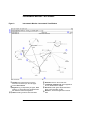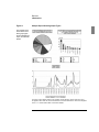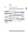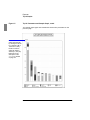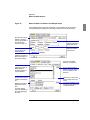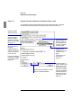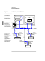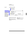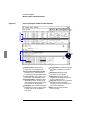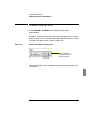
1
About this Manual
We’ve added this manual to the Agilent website in an effort to help you support
your product. This manual is the best copy we could find; it may be incomplete
or contain dated information. If we find a more recent copy in the future, we will
add it to the Agilent website.
Support for Your Product
Agilent no longer sells or supports this product. Our service centers may be able
to perform calibration if no repair parts are needed, but no other support from
Agilent is available. You will find any other available product information on the
Agilent Test & Measurement website, www.tm.agilent.com.
HP References in this Manual
This manual may contain references to HP or Hewlett-Packard. Please note that
Hewlett-Packard's former test and measurement, semiconductor products and
chemical analysis businesses are now part of Agilent Technologies. We have
made no changes to this manual copy. In other documentation, to reduce
potential confusion, the only change to product numbers and names has been in
the company name prefix: where a product number/name was HP XXXX the
current name/number is now Agilent XXXX. For example, model number
HP8648A is now model number Agilent 8648A.
User’s Guide
1
HP OpenView NetMetrix/UX
version 6.02
5967–9446
Introduction
The New World of
Network Management
Welcome to the new world of network management—a world where
you can clearly see what’s happening on your network, and it is no longer
a mystery or black box.
Is it a fantasy? Not with HP OpenView NetMetrix/UX.
NetMetrix clarifies what is happening on the network so that network
problems can be quickly isolated and potential problems corrected before
they become a problem. Gathering critical network information from a
wide variety of collectors and applications that analyze and report on the
data collected, NetMetrix provides the critical visibility into the network
to ensure network availability and responsiveness, and helps you:
● Increase network availability.
● Improve network performance and manage switch networks.
● Control network costs and justify network expenditures.
● Create and maintain network service level agreements.
● Use data collectors, your network informants.
● Extend the power of HP OpenView Network Node Manager.
Increase Network Availability
Today’s networks have become an integral part of the success of a business and provide a competitive advantage to the business. These are
business-critical networks. They are used to generate direct and indirect
sales, electronically order material from vendors on demand, make payments, and are essential to the overall productivity of the business.
With such a high demand placed on networks, it is imperative that network problems be corrected promptly. NetMetrix provides the tools
needed to quickly isolate and resolve network problems before network
availability is compromised.
2
5967–9446
HP OpenView NetMetrix/UX User’s Guide
Introduction
Improve Network Performance and Manage Switch Networks
The only thing worse than an unavailable network is a poorlyperforming network. NetMetrix can help you become more proactive in
managing your network performance, so that action can be taken before
performance becomes unacceptable or unavailable.
NetMetrix can make a difference by identifying potential bottlenecks,
providing trending information, helping with capacity planning, and predicting the impact of deploying a networked application on your network
before you actually deploy it onto your operational environment.
NetMetrix will help you focus on successful management of new highspeed, high-capacity technologies, such as switches, Fast Ethernet, and
ATM, allowing you to:
● Identify potential bottlenecks and network performance trends.
● Help with capacity planning.
● Determine the impact of deploying an application on your network.
● Manage switched network performance.
Control Network Costs and Justify Network Expenditures
The cost of network changes and outsourcing services such as WAN
takes a significant toll on the IT budget. For example, WAN outsourcing
is usually the third largest expenditure in the IT budget, just behind
payroll and capital expenses. Business is always looking for ways to
reduce costs and the IT budget is not exempt from this process.
How can you insure you are getting the maximum benefit from your network investment before incurring additional costs? How can you justify
additional network expenditures? NetMetrix can help you:
● Reduce WAN costs.
● Maximize network investments.
● Justify network expenditures.
5967–9446
3
HP OpenView NetMetrix/UX User’s Guide
Introduction
Create and Maintain Network Service Level Agreements
Networked environments have evolved and matured to the point where
focus has shifted from technology adoption and implementation issues to
management activities needed to support users’ business-critical environments. As a result, the strategic role that IT plays in delivering
business continuity across the enterprise has elevated.
Delivering consistent levels of network service to end-users becomes an
important part of network success. This process—known as network
service level management—requires IT to define, deploy, monitor, and
maintain required levels of IT performance and service to business users
of the enterprise. NetMetrix provides you with the tools to help define,
monitor, and maintain your level of network service.
Use Data Collectors, Your Network Informant
The visibility and detail available in NetMetrix applications require a
network informant known as a data collector. These collectors capture
information about the data flowing through the network area they monitor and forward this information to NetMetrix applications. NetMetrix
has two classes of data collectors—dedicated hardware probes and software agents.
Dedicated hardware probes are high-performing capturing devices dedicated to passively collecting network traffic. Each probe uses HP’s “nocompromise design” to provide the highest performance solution for the
given media to insure that data is always collected—even during times of
network saturation. After all, it’s during these critical times that detail is
most crucial, and NetMetrix’s high-performance collectors don’t miss a
beat.
Software agents capture information that provides greater visibility to
what is happening on the network between workstations, servers, and
switches. HP provides software agents that run on workstations or
servers, while embedded RMON is provided by switch vendors and
operates on their switches.
4
5967–9446
HP OpenView NetMetrix/UX User’s Guide
Introduction
Extend the Power of HP OpenView Network Node Manager
NetMetrix and Network Node Manager are the industry’s two leading
network management solutions in their respective areas. When combined, they provide the most powerful integrated network management
solution available in the industry today.
From one integrated OpenView solution, you get visibility into your network devices and topology, device availability tracking, monitoring/
prioritizing of events, and network traffic visibility. In addition you can
identify who are the top network consumers and what are the top applications being used, track utilization trends, monitor network availability
and responsiveness, isolate network problems, and report on the status
of your network. To offer this solution, NetMetrix integrates with Network Node Manager’s console and database to provide a single network
management environment from which you can perform both products’
functions.
A Wise Investment
HP is committed to providing the most comprehensive network management solution available to help you intelligently manage your businesscritical networks.
As a part of this solution, NetMetrix gives you the visibility, analysis,
and network reports needed to ensure network availability and responsiveness, manage switch network performance, control networks costs,
and manage network service agreements. With new complementary network management products in development and expanding on current
product capabilities, HP continues to provide the best tools needed to
keep your network moving at the speed of today’s business.
5967–9446
5
Reporter—At a Glance
Figure 1
Reporter: Status Window
➀
➁
➂
➃
➄
➀ Menu bar:
➁
➂ Report status area, with one report selected
File Menu contains items to create a new
report, open an existing report file, view the error
log, and exit the application.
Report Menu includes items that operate on
one or more selected reports: modify (page 56),
generate now (page 55) display now (page 54),
and remove (page 58).
Help Menu provides access to online
documentation for Reporter.
Toolbar gives quick access to common
functions:
creates a new report (page 58).
opens an existing report file (page 57).
modifies selected reports (page 56)
generates selected reports (page 55)
displays selected reports on screen
(page 54)
launches online documentation for Reporter
(page 59).
6
➃
➄
(highlighted).
Each line in the status area shows the report
owner’s username, the report file name, whether
the report is suspended, when the report is
scheduled, and where report output is directed.
The status information represents the Reporter
entries scheduled in cron, with some of the
information extracted from the report file.
Click to select a report; click and drag or Shiftclick to select contiguous reports; Ctrl-click to
select or deselect non-contiguous reports.
Assist line, which gives helpful information
about current operation or field.
Status line, shows the application’s current
state.
5967–9446
Figure 2
Reporter: Report Definition Window
Toolbar functions:
saves the report to a file
(page 69).
cuts the selected graph(s) to the
clipboard (page 74).
copies the selected graph(s) to the
clipboard (page 74).
pastes the contents of the clipboard
at the current location (page 74).
displays the schedule/output
window (page 67).
generates the report now
(page 55).
displays the report on screen
(page 65).
adds a Protocol Distribution,
Top N, Network Health,
Response Profile, or
Component Health graph
to the report (page 72).
➀
➁
➂
➃
➄
➅
➆
➇
➀ Toolbar gives quick access to common
➁
➂
➃
modifies selected graphs
(page 153).
launches online documentation for
Reporter (page 59).
functions; see summary at upper right.
Graphs comprising this report; including a
Network Health, Response Profile, Protocol
Distribution, and Top N. Two graphs are
selected. For a new report, this area is empty. To
add graphs, see page 72.
Page layout indicators specifying the number of
graphs for each page and how to arrange the
graphs on the page. See page 147.
Page header and footer definitions for the
report. See page 147.
5967–9446
➄ Scope determines whether data from several
➅
➆
➇
data sources is shown on the same graph or
separate graphs. See page 147.
Agents selection lists; determines the data
sources used for the report. See the close-up on
page 64.
Assist line, which gives helpful information
about the current operation or field.
Status line, shows the application’s current
state.
7
Internetwork Monitor—At a Glance
Figure 3
Internetwork Monitor: Internetwork View Window
➀
➁
➅
➃
➆
➂
➄
➇
➈
➀ Toolbar gives quick access to common
➁
➂
➃➄
functions; see close-up on the next page.
Current time interval.
Segment ring, as reported by an agent, ERM
instance, or archive file; lines represent traffic
flow between nodes and segments.
Labels showing node and line information.
8
➅ Protocols shown in the current view.
➆ “Collapsed” segment ring, which appears as
an icon; double-click to expand.
➇ Assist line, which gives helpful information
➈
about current operation or field.
Status line, shows the application’s current
state.
5967–9446
Figure 4
Internetwork Monitor: Internetwork View Window, Close-Up
➀
➁
➂
➀
➃
➄
Menu bar:
File Menu contains items to create, load, or save
a model (page 217); save or recall configuration
settings (page 242); print the current data
graphically or as a text report (page 237); and
view the error log (page 169).
Report Menu displays the current data as a text
table (page 182).
Properties Menu contains items for controlling
many aspects of the graphical view and the data
being displayed (page 189 and page 210).
View Menu contains items to display or remove
node and line labels (page 202), display an
information box for a selected item (page 203),
and create a new segment ring (page 218).
Monitor Menu contains an item to enable agents
or archives in the view (page 199).
Tools Menu lets you launch Load Monitor or
Protocol Analyzer against a selected object
(page 212).
5967–9446
➅
➁
➂
➃
➄
➅
➆
➆
Toolbar:
Create a model from this view (page 218).
Load a model (page 226).
Save the current model (page 225).
Print the current view (page 237).
Display the data report (page 182).
Pause the view, preventing any changes until
you resume (page 190).
Set the placement method: Address or Traffic
(page 172).
Change the view type: MAC layer (page 177),
Network layer (page 176), or Segment
(page 178).
Set the threshold (page 195).
Launches online documentation for Internetwork
Monitor.
To display a toolbar item’s Assist line, position the
mouse pointer over the item. The previous page
shows the Assist line for the view type pop-up (item
➄ on this page).
9
Load Monitor—At a Glance
Figure 5
Load Monitor: Base Window
Choose items from the
View menu to display
graphs of network load
Base window menus,
summarized below
Status area shows
information about
current data source/
instance
File Menu contains items to load data
from an archive file and view the error
log.
View Menu includes items to open
windows containing graphs that display
network load.
10
Attach… button lets you attach to a
different instance.
Help Menu lets you access on-line
documentation for Load Monitor.
5967–9446
Figure 6
Load Monitor: Zoom View
Current Zoom path
and pop-up menus
Use pop-ups to
change the path
Zoom path graphs:
Double-click in a
graph to select Zoom
focus point. The
graph title and a
dashed line indicate
the current zoom
point. Subsequent
graphs in the path
are updated to show
their status at the
selected zoom
point(s)
Zoom shows the relationships
between different aspects of network
traffic. The Zoom path indicates how
each graph progressively refines
the displayed information.
Zoom paths are built from these
elements:
• Source: nodes from which network traffic originates (“talkers”).
5967–9446
• Destination: nodes to which network traffic flows (“listeners”).
• Conversation: statistics between
pairs of nodes
• Protocol: link, network, transport,
and application layers.
• Time: network statistics as a
function of time.
• Size: traffic for different packet
size ranges.
11
Protocol Analyzer—At a Glance
Figure 7
Protocol Analyzer: Base Window
Base window menus,
summarized below
Click START to begin
packet capture
Status area gives
information about
current capture
instance
Click STOP to end
packet capture
File Menu contains items to save
captured data to or load data from a file,
save filters and settings to a file or recall
them, clear current filters/settings and
load the defaults, and display the error
log.
View Menu lets you open a decode
window of captured packets showing
summary, detail, and hex information or
a Traffic Trend graph of packet match
counts.
12
Filter Menu contains items to specify a
filter for controlling which packets are
captured.
Settings Menu contains items to
configure the capture buffer and indicate
which network interface to monitor.
Instance Menu lets you create, attach
to, remove, and post-filter packet capture
instances.
Tools Menu lets you launch the Alarms
application against the current data
source.
5967–9446
Figure 8
Protocol Analyzer: Packet Decodes Window
➅
➀
➁
➂
➃
➆
➇
➉
➄
➈
➀ Marked packet; double-click to
toggle mark, or use Marks menu
➁ Error packet, Information packet
indicates error or information bit is
set; Detail pane shows packet status
➂ Current packet; click to select, use ↑
and ↓ keys, or use Navigate menu
➃ Skipped packets; indicates a gap in
the packet numbers, usually occurs
when the buffer fills and wraps faster
than packets can be displayed
➄ Highlights show correlation between
Detail and Hex; click on part of packet
in either pane to see equivalent in
other pane
5967–9446
➅ Toggle buttons control which panes
are visible and whether to use auto
scroll
➆ Summary pane gives a brief
description for each packet
➇ Detail pane shows the current
packet’s decode; different layers are
shown in different colors
➈ Hex pane shows the current packet in
hexadecimal bytes and ASCII
characters; colors correspond to the
colors in the detail pane
➉ Sash controls height of panes
(close-up view)
13
RMON Utilities—At a Glance
Alarms and Traps
Alarms and traps let you configure
RMON agents to alert you when
interesting activity occurs on the
network. You define what “interesting activity” is, and you control
what happens when the agent
detects it.
For example, you might configure an
alarm to monitor octet counts per
second. When the count rises above
the value you specify, the alarm triggers and sends a trap—a message to
your management station—indicating that the count exceeded the
threshold you specified.
For details, see page 417.
Live Statistics
The RMON Utilities include several
tools for viewing live statistics.
Multi-Segment Statistics show
segment-level statistics from multiple agents on the same graph,
allowing you to compare statistics
from different segments with ease.
The statistics shown by this tool are
based on RMON’s Statistics group.
Node Statistics let you view the
entire node (host or station) table, or
you can display a graph of statistics
for specified nodes on the segment.
The statistics shown by this tool are
based on RMON’s Host group and
tokenRing Station table.
Traffic Matrix lets you view
activity between specified nodes as a
graph or a table of statistics. The
statistics shown by this tool are
based on RMON’s Matrix group.
Historical Statistics
(including Baseline)
Historical Statistics lets you view
past network activity and develop
baselines that help you discern
patterns of activity, trends in
behavior, and exceptional events.
By looking at short-term statistics,
you can identify network performance problems; long-term statistics
assist you in network configuration,
capacity planning, and network
segmentation.
Three studies can be viewed: hourly,
which shows data at 5-second intervals; daily, at 30-second intervals;
and monthly, at 30-minute intervals.
You can also access historical data in
files created by the collector daemon,
allowing you to view long-term
trends and calculate baselines.
Baselines combine historical
measurements with statistical
algorithms to analyze network data.
In particular, baselines:
• Highlight exceptional activity,
helping to pinpoint network
problems.
• Show network patterns, helping
you discover what’s normal for
your site. This information is
useful when setting alarms that
trigger when something is
abnormal.
• Reveal long-term trends, which is
useful when planning expansions
and purchasing equipment based
on utilization growth.
For details, see page 475.
For details, see page 455.
14
5967–9446
Token Ring Applications
LanProbe IP Address Tracking
The RMON Utilities include several
tools specifically for token ring
networks.
LanProbe IP Address Tracking lets
you match MAC addresses and IP
addresses as seen by an HP
LanProbe.
Ring Status displays descriptive
information about one or more token
ring networks.
Ring Order shows information
about which stations are currently
active and which stations were once
active but have dropped out or been
removed from a token ring network.
Source Routing Statistics
displays a graph showing source
routing activity on a token ring,
letting you see how many hops
individual frames traverse.
Remove Station lets you remove a
specified member from a token ring
network, allowing you to eliminate a
station that is causing problems on
the ring.
Ring Entry Errors displays a table
of entry error statistics for one or
more token ring networks.
For details, see page 491.
Protocol Distribution
Protocol Distribution displays pie
graphs of the top protocols used on
your network, based on data collected by a standard RMON agent.
For details, see page 511.
RMON Log Table
RMON Log Table lets you view the
log table entries for an agent.
For each log entry, RMON Log Table
creates a line with the event index,
the log index, the time the event
fired and the log description associated with that event. RMON Log
Table includes filter capabilities that
let you sort the log table, view only
selected events, or restrict the displayed entries to a specified time
range.
For details, see page 515.
RMON Status
RMON Status retrieves status information from an agent. It displays the
values of all instances of control
table entries for an RMON group.
You can choose which group to
display.
For details, see page 523.
For details, see page 503.
5967–9446
15
Applications and Agents
Table 1 on page 18 lists all of the applications in the HP OpenView NetMetrix/UX suite and indicates which agents are supported.
LanProbe
J3458A HP Fast Ethernet LanProbe
J3457A HP Quad Ethernet LanProbe
4986B HP Ethernet LanProbe
4987B HP Ethernet LanProbe with AUI
J3911A HP Multiport Token-Ring LanProbe
4985A HP Token-Ring LanProbe
4985B HP Token-Ring LanProbe
J332xB HP FDDI LanProbe with Ethernet Telemetry,
J332xA HP FDDI LanProbe.
WanProbe/
ATMProbe
J3914A HP E1 WanProbe
J3913A HP T1 WanProbe
J3915A HP V-Series WanProbe
J3919A, J3972A HP OC-3 ATMProbe
J3918A, J3971A HP UTP ATMProbe
J3920A, J3973A DS-3 ATMProbe
J3921A, J3974A E3 ATMProbe
J3917A T3/DS-3 WanProbe
Extended RMON
Module (ERM)
HP-UX or Solaris workstation running NetMetrix Extended RMON
Module software.
PVC
A permanent virtual circuit (PVC) configured on an HP WanProbe or
HP ATMProbe.
Cisco ISL VLAN
An Cisco Inter-Switch Link Virtual LAN configured on a full-duplex HP
Fast Ethernet LanProbe.
Cisco Switch
Cisco Catalyst 5000 and Cisco Catalyst 5500 switches with RMON
enabled. The mini-RMON agent implemented by these switches
supports the Statistics, History, Alarm, and Event RMON groups for
Ethernet, Fast Ethernet, and Token Ring (copper and fiber) ports.
16
5967–9446
HP OpenView NetMetrix/UX User’s Guide
Applications and Agents
HP ProCurve
Switch
J4110A ProCurve Switch 8000M
J4120A ProCurve Switch 1600M
J4121A ProCurve Switch 4000M
J4122A ProCurve Switch 2400M
J3298A ProCurve Switch 212M
J3299A ProCurve Switch 224M
J3301A ProCurve Switch 10base T Hub12M
J3303A ProCurve Switch 10base T Hub 24M
J3288A ProCurve Switch 10T/100T Managed 12-Port Hub
J3289A ProCurve Switch 10T/100T Managed 24-Port Hub
J4093A ProCurve Switch 2424M
Extended Data
Source (DS)
A device other than the ones listed above that implements the
NetMetrix RMON Extensions (or the HP EASE MIB) and has been
associated with an ERM.
Examples include older HP WanProbes and HP LanProbes, and HP
AdvanceStack hubs and routers.
RMON Data
Source (DS)
A device other than the ones listed above that implements the RMON
standard. (While RMON is a standard, the implementation of each
vendor’s RMON agent is slightly different; as a result, NetMetrix may
not operate completely with every “standard” RMON agent.)
Also includes older HP LanProbes.
5967–9446
17
HP OpenView NetMetrix/UX User’s Guide
Applications and Agents
Application
Wan/ATMProbe
ERM
PVC
ISL VLAN
Cisco Switch
HP Procurve
Extended DS
RMON DS
NetMetrix Applications and Agents
LanProbe
Table 1
Reporter
●
●
∅
●
●
●
●
●
● WanProbe, ATMProbe, and PVC
Notes
data sources must be associated
with an ERM. Available graphs
depend on configured data
collection. Also works with
Internetwork Response Agents
(IRAs) and network
components.
Internetwork Monitor
●
●
●
●
●
∅
●
●
∅ Data source must be associated
with an ERM. To use a PVC, the
end points must be configured in
Agent Manager.
Load Monitor
Extended RMON views
Standard RMON views
●
●
Protocol Analyzer
●
Extended RMON views require
●
∅
●
∅
●
∅
●
●
●
∅
●
●
∅
●
∅
●
●
∅
●
∅
∅ that the data source be
● associated with an ERM. For
∅
● Requires Filter and Capture
standard RMON views, the
RMON tables may require
initialization. Uses Statistics,
History, Host, HostTopN, and
Matrix RMON groups. Some
features depend on agent; refer
to page 337.
RMON groups.
Legend:
● Application is supported. Specific application features may depend on the agent’s capabilities.
∅ Application is not supported.
18
5967–9446
HP OpenView NetMetrix/UX User’s Guide
Applications and Agents
Application
Wan/ATMProbe
ERM
PVC
ISL VLAN
Cisco Switch
HP Procurve
Extended DS
RMON DS
NetMetrix Applications and Agents, continued
LanProbe
Table 1
Alarms and Traps
●
●
∅
●
●
●
●
∅
● Requires Alarm and Event
Notes
RMON groups. Traps require an
event manager, such as HP
OpenView Network Node
Manager.
Trap Destinations
●
●
∅
∅
∅
∅
∅
∅
∅
Live Statistics
●
∅
∅
∅
∅
●
●
∅
● Ethernet and token-ring data
sources only. Uses Statistics,
Host, and Matrix RMON
groups. Since Cisco agents do
not implement the Host and
RMON tables, Node Statistics
and Traffic Matrix are not
supported for Cisco Switch.
●
Historical Statistics
∅
∅
∅
∅
●
●
∅
● Ethernet and token-ring data
sources only. Requires History
RMON group. Uses RMON
data collection, if available.
Token Ring Applications
●
∅
∅
∅
∅
∅
∅
∅
● Token ring data sources only.
Requires Token Ring RMON
group.
Protocol Distribution
●
●
∅
●
●
∅
∅
∅
● Requires Filter and Capture
RMON groups.
∅
∅
∅
∅
∅
∅
∅
∅ Most older LanProbes will also
LanProbe IP Address
Tracking
●
RMON Log Table
●
●
∅
∅
∅
●
●
∅
●
RMON Status
●
●
∅
∅
∅
●
●
∅
●
work, except for 4985A.
Legend:
● Application is supported. Specific application features may depend on the agent’s capabilities.
∅ Application is not supported.
5967–9446
19
HP OpenView NetMetrix/UX User’s Guide
Applications and Agents
Agent Administration:
Warm/Cold Start
Authentication
LanProbe Configuration
Download Firmware
PVC
ISL VLAN
Cisco Switch
HP Procurve
Extended DS
RMON DS
Internetwork Response
Manager
ERM
Application
Wan/ATMProbe
NetMetrix Applications and Agents, continued
LanProbe
Table 1
●
∅
∅
∅
∅
∅
∅
∅
∅ Requires up-to-date firmware on
Notes
the probe. Also works with IRA.
Refer to DNA User’s Guide for
details.
Refer to Data Collector
●
●
●
●
●
●
●
●
●
●
∅
∅
∅
∅
∅
∅
∅
∅
∅
∅
∅
∅
∅
∅
∅
∅
∅
∅
∅
∅
∅
∅
∅ Reference for details on these
applications.
∅
∅
∅
Legend:
● Application is supported. Specific application features may depend on the agent’s capabilities.
∅ Application is not supported.
20
5967–9446
HP OpenView NetMetrix/UX User’s Guide
Applications and Agents
In This Book
The following summarizes the HP OpenView NetMetrix/UX documentation set, which gives detailed information about the NetMetrix software
suite.
Document
Description
Installation
Installation and configuration of the
NetMetrix/UX software suite, including a
troubleshooting section and information on
licensing.
Data Collector
Reference
Agent Manager, Agent Administration,
Collector Daemon, Extended RMON Module
(ERM).
This Book ☛ User’s Guide
DNA User’s Guide
Reporter, Internetwork Monitor, Load
Monitor, Protocol Analyzer, Alarms and Traps,
Live Statistics, Historical Statistics, and other
RMON utilities.
Distributed Network Analysis: Internetwork
Response Manager (IRM), Internetwork
Response Agent (IRA).
Before continuing, ensure that you have installed the HP OpenView NetMetrix/UX software. Instructions are included in Installation.
The online version of the various chapters of this manual contain red
links (which jump to locations within the manual) and blue links (which
jump to locations in other manuals).
For more information on Netmetrix, visit our website at http://
www.hp.com/go/netmetrix.
5967–9446
21
HP OpenView NetMetrix/UX User’s Guide
Applications and Agents
22
5967–9446
Contents
User’s Guide
Introduction 2
Reporter—At a Glance 6
Internetwork Monitor—At a Glance 8
Load Monitor—At a Glance 10
Protocol Analyzer—At a Glance 12
RMON Utilities—At a Glance 14
Applications and Agents 16
Reporter
35
Introduction
36
Graph Types 37
Required Data 42
Temporary Files 44
About LOW-CONTRIB, TCP-other, and UDP-other
Reporter’s Web Interface 46
Baselines 47
What You Need 49
Running Reporter
45
50
To start Reporter in demonstration mode 51
To start Reporter 52
To display the results of selected reports on the screen
To print a displayed report 55
To generate selected reports now 55
To modify selected reports 56
To open a report that’s not shown 57
To create a new, blank report 58
To remove selected reports 58
5967–9446
54
23
User’s Guide
Contents
To learn more about Reporter
To view the error log 59
To exit Reporter 60
Creating Reports
59
61
To create a new report from a sample report 62
To select data sources 64
To display the report on the screen 65
To save a sample report with a different name 66
To schedule a report and specify the output 67
To generate the report 69
To save a report 69
To create a new report from scratch 70
Manipulating Graphs
71
To add graphs to a report 72
To modify selected graphs 73
To remove a graph 73
To insert a new graph before an existing graph 74
To rearrange the graphs in the report using cut/copy and paste
Protocol Distribution Graphs
75
To configure a Protocol Distribution graph
Top N Graphs
76
79
To configure a Top N graph
80
Network Health Graphs
83
To configure a Network Health graph
Response Profile Graphs
84
105
To configure a Response Profile graph 106
Target Names 112
Graph Configuration for Response Profile Targets
24
74
112
5967–9446
User’s Guide
Contents
Component Health Graphs
114
To configure a Component Health graph 115
To Create Custom Component Categories 123
Scheduling Reports
125
To schedule on one day per week 126
To schedule at the same time on more than one day per week 127
To schedule on the same day and time for one or more months 128
To set a custom schedule 129
To suspend a report 131
To activate a suspended report 131
Setting Up Report Output
132
To send output to a printer 133
To send output to an X display 134
To save output in a file 135
To send output as electronic mail 136
To process output with a command 137
Exception Reporting
139
To define a graph’s exception criteria 140
Static Threshold exception criteria 140
Auto-Adjusting Baseline exception criteria
Valid report configurations 142
Designing report pages 144
To disable a graph’s exception criteria 145
Tailoring a Report’s Appearance
140
146
To set the page layout parameters 147
Special Variables: DISPLAY, LPDEST, PRINTER
To change the graph settings 153
To specify the graph style 158
To select a font 160
5967–9446
148
25
User’s Guide
Contents
Internetwork Monitor
161
Running Internetwork Monitor
To access live data 164
To access archive files 166
To view the error log 169
To exit Internetwork Monitor
169
Viewing the Internetwork
170
163
Placement: Assigning Nodes to Segments 170
Views: Network Layer, MAC Layer, or Segment
To set the placement method 172
Address Placement 172
Traffic Placement 175
To view end-to-end traffic patterns 176
To view traffic within and across segments 177
To view intersegment traffic patterns 178
To view the data values being displayed 182
Color and Line Styles 187
Icons in the internetwork view 188
Controlling the Data in the View
171
189
To pause the view 190
To change the displayed time interval 191
To change how often graphs are updated 193
To change what data is displayed 194
To set the threshold 195
To filter data by protocol 197
To enable monitoring for a new data source 199
Manipulating the View
200
To select items 201
To display labels 202
To remove labels 203
To display information boxes 203
To move a segment ring or icon 205
26
5967–9446
User’s Guide
Contents
To resize a segment ring 206
To collapse or expand a segment ring
To rotate a segment ring 207
To move nodes 208
To tailor the graphical display 210
207
Launching Other Tools 212
To launch Load Monitor from Internetwork Monitor 213
To launch Protocol Analyzer from Internetwork Monitor 215
Traffic Profile Modeling
217
To create a model 218
To create a new segment ring in the view
To manipulate a model 219
To save a model 225
To load a model 226
Interpreting the Internetwork View
218
227
Node-to-Segment Assignments 227
Address Placement 228
Traffic Placement 228
Interconnect Devices 229
Nodes on Unmonitored Segments 229
Data Integration, Network Layer View 230
Data Integration, Segment View 231
Data Integration, MAC Layer View 233
Routed Traffic 233
Non-Routed Traffic 235
Printing and Saving Data
237
To print or save the graphical view 238
To print graph(s) in color 240
To print or save the data report 241
5967–9446
27
User’s Guide
Contents
Working with Properties Files
242
To save properties in a file 243
To load a properties file 243
To tailor the default properties 243
Load Monitor
245
Running Load Monitor
247
To access extended RMON data 248
To access standard RMON data 251
To run Load Monitor for an archive file
To view a different instance 256
To view the error log 256
To exit Load Monitor 257
Displaying Load
254
258
To open a view window 258
Special Entries: Others, LOW-CONTRIB, TCP-other, and UDP-other
To use Zoom 262
Zoom Elements and Paths 264
Zoom Pop-Up Menus 265
Useful Zoom Paths 266
To view a Conversation segment graph 272
To rotate a segment graph 273
To search for a data point 274
To expand or contract the X or Y axis 276
Expand 277
Contract 277
Accumulate 277
To accumulate time values with the graph pop-up 282
Changing Properties
284
Data Properties 284
Graph Properties 286
To change how often graphs are updated 288
To change what data fields are displayed 289
28
5967–9446
259
User’s Guide
Contents
To sort data 293
To filter data 295
To set the Zoom layout 298
To change a graph’s appearance 299
To modify a graph’s scale 301
To save properties in a file 303
To load a properties file 303
To tailor the default properties 304
Statistics
305
Working with Collected Data
333
To print or save the graph(s) in the view window
To print graph(s) in color 335
To print or save a text report 335
To load an archive file 336
Availability of Features
334
337
Extended RMON Data 338
Standard RMON Data 338
Zoom Element Views 338
Protocol Analyzer
339
Running Protocol Analyzer
341
To run Protocol Analyzer 342
To view the error log 345
To exit Protocol Analyzer 346
Using Packet Capture Instances
347
To create a new packet capture instance
To attach to an existing instance 350
To remove an instance 352
To start an instance 353
To stop an instance 354
5967–9446
349
29
User’s Guide
Contents
To arm an instance 355
To configure the capture buffer 356
To slice packets 357
To specify which network interface to use 357
To capture on multiple network interfaces simultaneously
Building a Filter
358
360
Filter Component Windows 360
Filter Expression Language 361
To filter by host 362
Specifying Hosts 362
To filter by protocol 366
To filter by packet status 369
To filter by matching a pattern 371
To specify a filter expression 376
Filter Expression Syntax 376
Description of Terms 379
Working with Captured Packets
380
To view packets 381
Window Panes 383
Scrolling 383
Navigation 384
Error and Information Packets 385
To mark packets 386
To unmark packets 386
To search for a packet 387
To tailor the Summary pane 389
To print or save a report of captured packets 392
To save captured packets in a trace file 393
To load a trace file 394
To reload packets from the capture buffer 394
To post-filter captured packets 395
To display Traffic Trend (packet match counts) 396
Working with Configuration Files
To save filter/settings in a file
30
399
400
5967–9446
User’s Guide
Contents
To load a filter/settings file 400
To load the default filter/settings 401
To tailor the default filter/settings 402
To save properties in a file 403
To load a properties file 403
To tailor the default properties 404
Using the protanal Command
Protocol Decodes
405
407
Alarms and Traps
Configuring Traps
417
419
To manage trap groups 420
To add a trap group or destination 423
Network Trap Destinations 423
Serial Trap Destinations 425
To modify a trap destination 427
To remove a trap destination or group 428
HP Probe-Specific Events/Traps 429
Setting Alarms
430
To manage alarms 431
To configure an alarm 433
Thresholds 436
To modify an alarm 438
To remove an alarm 438
To set different rising and falling thresholds 439
To control what happens when an alarm triggers 441
Alarms and Packet Capture Instances 444
Examples 444
About Alarm Owner Strings 450
Trap Handling 451
To display an alarm’s log 452
5967–9446
31
User’s Guide
Contents
Live Statistics
455
Multi-Segment Statistics
457
To display multi-segment statistics
Node Statistics
458
461
To display a graph of node statistics 462
To display a table of node statistics 465
To export statistics to a file 467
Traffic Matrix
468
To display the traffic matrix graph 469
To display Traffic Matrix as a table 472
To export statistics to a file 474
Historical Statistics
Displaying Statistics
475
477
Available Statistics 478
Interpreting Data Loss 479
To display the hourly study 480
To initialize the hourly study 482
To display the daily study 483
To display the monthly study 484
Using Baselines
485
Measurements 485
Methodology 485
High and Low Baselines 486
Cumulative Averages 487
To display the monthly baseline 488
To display the yearly baseline 490
32
5967–9446
User’s Guide
Contents
Token Ring Applications 491
To display token ring status 493
To display token ring order 495
To display source routing statistics 497
To remove a station from the ring 498
To display token ring entry errors 500
To export token ring entry errors to a file
Protocol Distribution
501
503
To display the distribution graph 505
Special Entries: Other, TCP-other, and UDP-other 506
To indicate how frequently to generate a new snapshot 507
To pause the application 508
To select the graph units 509
To view the error log 510
To exit Protocol Distribution 510
LanProbe IP Address Tracking
To display the IP Table
RMON Log Table
513
515
To display the log table 517
To sort the log table 518
To control the displayed time range
To filter by event 519
To view the error log 521
To exit RMON Log Table 521
RMON Status
511
519
523
To display status information 524
To display the status for a different RMON group
To view the error log 526
To exit RMON Status 526
5967–9446
525
33
User’s Guide
Contents
Graphs and Tables
527
Working with Graphs
528
To control what statistics are shown and how 530
To change the display interval and resolution 532
To view statistics for the graph 534
To tailor the graph’s appearance 535
Working with Data Tables
537
To sort a table 538
To print a table 539
To save a table 539
Index
34
541
5967–9446
User’s Guide
Reporter
5967–9446
Reporter
Introduction
HP OpenView NetMetrix/UX Reporter lets you create and schedule
reports showing your network activity and responsiveness. Once you
have configured a report, it is generated automatically, according to the
schedule you set, without further intervention.
A report consists of one or more graphs arranged on pages, using data
collected from data sources and stored in data files on your management
station. You indicate which graphs you want in your report, how to
arrange them on the page, and what data sources’ data to depict.
Reporter’s graph types are discussed below.
You can generate a report for one data source or several. If you create a
report for multiple data sources, you choose whether to have the data
from each data source graphed separately or have all sources’ data
shown in a single graph, allowing easy comparison.
In addition to defining a report’s contents, you also specify the schedule
for report generation. For example, you might have some reports that are
generated daily, once a week, several times a month, or once a year. The
schedule you specify is translated into a crontab entry, which is then
executed by cron. Once the schedule is set, you don’t need to do anything
else; the reports are sent to the output destination you define.
For each report, you can request that the output be printed, saved in a
file, displayed to the screen, sent as electronic mail, or processed by a
command that you specify. This flexibility ensures that the report results
are delivered in the manner that suits you best.
Reports can also be published on the World Wide Web. For information,
refer to page 46 and to the file /usr/netm/www/README.www.
36
5967–9446
Reporter
Introduction
Graph Types
Reporter provides five basic types of graphs:
●
Protocol Distribution graphs let you see the protocol mix on your
network.
You can request a graph showing all data in aggregate (a single data
value for each protocol for the entire time span), or ask for a graph
showing protocol use over time, using the interval you specify. In addition, you can limit the graph to the protocols used most often.
●
Top N graphs show the top talkers (source hosts), top listeners (destination hosts), or top pairs (conversations between two hosts).
As with Protocol Distribution, you can request a graph showing all data
in aggregate (a single data value for each talker, listener, or pair for the
entire time span), or ask for a graph showing values over time, using
the interval you specify.
You can also request a protocol breakdown for each host, showing the
protocols used most or a single specified protocol.
●
Network Health graphs show network statistics over time, based on
30-second or 30-minute intervals. In addition, you can choose to graph
a baseline for a particular statistic. These graphs are similar to the
Historical Statistics daily and monthly options described in “Historical
Statistics” on page 475.
The available statistics depend on the media type: Ethernet, tokenring, FDDI, or WAN. Note that there are many kinds of statistics available for WAN.
●
Response Profile graphs show response measurement data over time
for targets created on LANProbes or IRAs by Internetwork Response
Manager (IRM), using 5- or 30-minute intervals. You can choose to
graph average response time, conformance of average response to a
specified value, minimum and maximum response times, availability
percentage, and retransmission percentage. In addition, you can choose
to graph a baseline for a particular statistic.
Response Profile graphs are available only for HP-UX.
5967–9446
37
Reporter
Introduction
●
Component Health graphs show network component statistics over
time, based on 5- or 30-minute intervals. In addition, you can choose to
graph a baseline for a particular statistic. These graphs are based on
data collected from network component MIBs by HP OpenView Network Node Manager’s snmpCollect utility.
The available statistics depend on the component category. Reporter
includes statistics for Cisco Routers, Cisco Router Interfaces, and
Universal MIB.
Component Health graphs are available only if HP OpenView Network
Node Manager is installed on the Reporter host.
Figure 9 on page 39.
38
5967–9446
Reporter
Introduction
Figure 9
Sample Report Showing Graph Types
This sample report
shows three of the
basic graph types:
Protocol Distribution,
Top N, and Network
Health
For clarity, most reports shown in this chapter use fill patterns, rather than colors, and
2D graphs, rather than 3D. These characteristics are controlled with X resources configured
in the Netm resources file. Refer to the file for details.
5967–9446
39
Reporter
Introduction
Figure 9
Sample Report Showing Graph Types, cont’d
This sample report
shows a Response
Profile graph with
average response
time for two targets
40
5967–9446
Reporter
Introduction
Figure 9
Sample Report Showing Graph Types, cont’d
This sample report
shows a Component
Health graph
5967–9446
41
Reporter
Introduction
Required Data
Reporter bases its graphs on data collected from data sources on your
network and stored in data files on the management station. In order to
create reports, you first need to configure agents, data sources, and data
collection in Agent Manager.
Four types of data collection can be configured:
● RMON, which is based on the History group. For FDDI, RMON data
collection is based on a History-like group in HP’s private MIB.
● Extended RMON, based on NetMetrix RMON extensions.
● Response, based on targets configured with Internetwork Response
Manager (IRM).
● Component, based on MIBs for network components or elements.
Table 2 on page 43 indicates what kind of data is needed for each of the
available graph types.
For information on configuring data collection for your data sources,
refer to the Agent Manager chapter in Data Collector Reference.
42
5967–9446
Reporter
Introduction
Table 2
Required Data for Graphs
Graph
Data Type
Protocol Distribution
mix of protocols in use
Extended RMON
Top N
top talkers, top listeners, top conversation
pairs
Extended RMON
Network Health: WAN, PVC
link statistics over time; with or without
baseline
Extended RMON
Network Health: Ethernet, Token-Ring,
FDDI, full-duplex Fast Ethernet,
ISL VLAN
segment statistics over time; with or
without baseline
RMON
Response Profile
Response
available only for HP-UX
response and availability measurements
over time; with or without baseline
Component Health
Component
available only if HP OpenView Network Node
Manager is installed
Cisco Router, MIB-II, or other MIB
statistics over time; with or without
baseline
5967–9446
43
Reporter
Introduction
Temporary Files
Reporter uses temporary files for several purposes, including merging
data from multiple data files, writing out X resources used to produce
reports, and writing the report output.
Temporary files are created in directory defined by the environment variable TMPDIR. If the variable does not exist, /var/tmp is used, and the
bigM.* and ldmp.* are placed in the /var/tmp/netmrep hierarchy.
Temporary files created by Reporter use the following file name formats:
bigM.*
Contains the results from merging multiple extended RMON
data files.
The size of these files depends on the requested duration for
the report. The longer the duration, the larger the number of
individual files to be merged, and the more space required for
this temporary file.
When a report is generated or displayed, one bigM.* file is
created, then deleted, for each Protocol Distribution or Top N
graph.
cron*
Holds changes to the user’s crontab file.
dat.*
Holds the data passed to the grapher process; used to
construct the graphs comprising a report. One file is created
for each graph when a report is generated or displayed.
ldmp.*
Contains text output derived from extended RMON data files
rep.*
Contains the report output file, in PostScript, XWD, or text
format. (You can reference this file within a report by using
the variable $OUTPUTFILE, discussed on page 149.) If you
specify output to a named file, the rep.* file is not created.
xres.*
Contains X resources that are passed to grapher process; these
resources control the appearance of graphs in a report. One
file is created when a report is generated or displayed.
44
5967–9446
Reporter
Introduction
Reporter cleans up its temporary files once they are no longer needed.
(As discussed on page 137, a temporary report output file is not deleted
automatically if the output is processed by a command.)
You can suppress the clean up of temporary files by running Reporter
with a debug logging level of 5. For details, refer to the man pages for
reporter(1) and reportgen(1).
About LOW-CONTRIB, TCP-other, and UDP-other
Reporter graphs may include some special entries: LOW-CONTRIB,
TCP-other, and UDP-other.
The LOW-CONTRIB item accounts for any hosts or protocols that are not
identified individually or cannot be decoded by Extended RMON Module
(ERM). The mechanism that assigns less-significant entries to LOWCONTRIB is dynamic. As such, the hosts or protocols represented by
LOW-CONTRIB may vary over the duration of a report. For details, refer
to the Extended RMON Module chapter in Data Collector Reference and
to the netmd.config file.
TCP-other and UDP-other represent a range of TCP or UDP protocols.
The range is defined in the configuration file ipport.equiv, but may be
overridden by the file sysprotolist on the ERM host.
By default, protocols that use TCP ports 512 through 65535 are combined into the TCP-other entry, and protocols that use UDP ports 512
through 65535 are combined into the UDP-other entry. Protocols in the
NetMetrix built-in list and those that are specifically enumerated in the
sysprotolist file are not affected by the ranges set in ipport.equiv
and will be processed as individual entries.
You can change the configured range by editing ipport.equiv, as discussed in the Extended RMON Module chapter in Data Collector
Reference and in the ipport.equiv file.
5967–9446
45
Reporter
Introduction
Reporter’s Web Interface
Reporter includes a Web interface that provides World-Wide-Web access
to reports generated automatically by Reporter. All of the Web-related
Reporter files—including scripts, documentation and configuration information—are installed in the directory tree /usr/netm/www.
The basic building block of Reporter’s Web interface is the domain. Each
Reporter Web domain lets you publish usage reports for the local and
wide area networks within that domain. In addition, a unique “networks
at a glance” report gives a quick overview of all the networks available in
domain. For each network, you can see a representation of activity for
the day, with any trouble spots clearly identified.
A Reporter Web domain system consists of the following software:
● A Web server, such as Apache or Netscape’s FastTrack.
● NetMetrix, specifically the collector daemon and Reporter, including its
Web-related files.
● Supporting utilities, including Perl and NetPBM. These utilities are
freely available on the Internet; compiled binaries are also included on
an unsupported, “as-is” basis with the Reporter package.
You can set up multiple Reporter Web domain systems throughout an
enterprise-wide network, then use a Web browser to view reports on any
of these domains.
For details, including a link to the Reporter on the Web demonstration,
point your Web browser at file:///usr/netm/www/README.html.
46
5967–9446
Reporter
Introduction
Baselines
Reporter’s Network Health, Response Profile, and Component Health
graphs include a baseline feature. Baselines are useful in determining
what is normal for your network which, in turn, helps you identify
abnormal events. This information is helpful, for example, when setting
alarm thresholds.
Reporter depicts the baseline as a colored area behind the line graph,
which shows the actual data values for the selected statistic. The baseline area represents the envelope between low and high baseline values,
which are based on data from the previous sixteen weeks.
The actual data values (which are not part of the baseline calculation)
are superimposed on the baseline envelope, allowing for easy
comparison.
A sample Network Health graph with baseline is shown on page 88.
To determine the baseline, Reporter compares a given data point to
similar 30-minute data points for the past sixteen weeks (if available),
calculates the standard deviation using the requested confidence level,
and graphs an envelope about that point.
A “similar” data point is one that represents the same period of the day
on the same weekday. The period used depends on the duration shown in
the graph:
● For reports showing one day or less, one-hour periods are used. For
example, Reporter combines the data for 8:00 am to 9:00 am Monday
morning and compares it with the data from previous Mondays
between 8:00 am and 9:00 am.
● For reports showing more than one day and less than one month, eighthour periods are used. For example, Reporter combines the data for
8:00 am to 4:00 pm Wednesday and compares it with the data from
previous Wednesdays between those hours.
● For reports showing more than one month, one-day periods are used.
For example, Reporter combines the data for all of Friday and compares
it with the data from previous Fridays.
5967–9446
47
Reporter
Introduction
As mentioned, Reporter uses up to sixteen weeks of historical data to
calculate the baseline. In addition, even if the graph itself is configured
to use 30- or 300-second data, the baseline is calculated from 30-minute
data.
If sixteen weeks of data have not been collected, Reporter uses whatever
data is available. If less than a week of data has been collected, Reporter
warns you that the available data is not sufficient to calculate a baseline,
and the graph is drawn without the baseline envelope.
You can control the baseline calculation by specifying the confidence
level. By default, a 90% confidence level is used, which means that 90%
of past measured values are within the baseline envelope (between the
low and high baseline values). A higher confidence level results in an
envelope that encompasses more of the past data values, typically
resulting in fewer exceptions shown on the graph.
You can also configure an exception report based on the baseline calculation; in this case, the report page is printed only when the actual values
are outside the baseline a specified percentage of the time. For details,
refer to page 139.
48
5967–9446
Reporter
Introduction
What You Need
Before using Reporter, check the following:
❏ Verify that all of the data sources—including components and IRAs—that
you want to use are defined in Agent Manager and that you have configured
appropriate data collection for each. Refer to the Agent Manager chapter in
Data Collector Reference for information about defining data sources and
configuring data collection. Table 2 on page 43 lists the kind of data
collection required for each Reporter graph type.
❏ Verify that community strings for all of the components and IRAs that you
want to use are configured using Network Node Manager’s xnmsnmpconf
utility.
❏ Check that cron is running on your system.
❏ Note that to use cron, you must have root capability. Check with your
system administrator before scheduling jobs with cron. Verify that your
user name is configured in the cron.allow file, if the file exists. If this file
does not exist, verify that your user name is not in the cron.deny file.
● For HP-UX, these files are located in /var/adm/cron/.
● For Solaris, these files are located in /etc/cron.d/.
If you do not have these prerequisites, you can use Reporter in demonstration mode, discussed on page 51.
5967–9446
49
Running Reporter
Reporter includes a graphical user interface that lets you define and
schedule reports of network activity.
To use Reporter to create and schedule reports based on your own network’s activity, ensure that you have checked the required items on the
previous page. In particular, ensure that you are collecting data from the
data sources you want to use with Reporter.
If you have not configured data collection (or if insufficient amounts of
network data are available), you can run Reporter in demonstration
mode, which lets you use Reporter’s capabilities with sample data
sources, data, and report definitions.
When you launch Reporter, the Report Status window opens; this
window gives a summary of all the reports currently defined and
scheduled. From this status window, you can:
● Display the results of a report on the screen.
● Generate a report according to the configured output parameters.
● Open an existing report file that isn’t scheduled and does not appear in
the status window.
● Remove reports; this operation removes the corresponding scheduling
information from your crontab file, but does not affect the report
definition file.
● Create a new report or modify an existing one.
These operations are discussed on the following pages.
50
5967–9446
Reporter
Running Reporter
To start Reporter in demonstration mode
●
From Agent Manager or OpenView NNM, choose
Misc ➤ HP NetMetrix Demonstration ➤
Internetwork Reporting…
Reporter’s demonstration mode lets you experiment with Reporter’s
capabilities using sample data sources, network data, and report definitions. Demo mode does not require any agent, data source, data
collection, or cron set up.
When you start Reporter in demo mode, the demo version of the Report
Status window opens. This window looks much like the one shown in
figure 10 on page 53.
Within demo mode, you can create new reports or open existing ones,
modify the demo reports, and display or generate report output based on
demo data. However, you cannot save reports.
The reports shown in demo mode are also available as sample files. As
discussed on page 61, these sample reports can be modified for your own
use (when not in demo mode).
See Also
“Creating Reports” on page 61.
“To open a report that’s not shown” on page 57.
“To display the results of selected reports on the screen” on page 54.
“To generate selected reports now” on page 55.
5967–9446
51
Reporter
Running Reporter
To start Reporter
●
Important
From Agent Manager or OpenView NNM, choose
Performance ➤ Internetwork Reporting…
Before using Reporter with data sources on your network, ensure that
you have checked the required items on page 49.
When you start Reporter, the Report Status window opens. A sample of
this window is shown in Figure 10 on page 53.
52
5967–9446
Reporter
Running Reporter
Figure 10
Report Status Window
➀
➁
➂
➃
➄
➀ Menu bar:
➁
➂ Report status area, with one report selected
File Menu contains items to create a new
report (page 70), open an existing report
file (page 57) view the error log (page 59), and
exit the application (page 60).
Report Menu includes items that operate on
one or more selected reports: modify (page 56),
generate now (page 55) display now (page 54),
and remove (page 58).
Help Menu provides access to online
documentation for Reporter.
Toolbar gives quick access to common
functions:
creates a new report (page 58).
opens an existing report file (page 57).
modifies selected reports (page 56).
generates selected reports (page 55).
displays selected reports on screen
(page 54).
launches online documentation for Reporter
(page 59).
5967–9446
➃
➄
(highlighted).
Each line in the status area shows the report
owner’s username, the report file name, whether
the report is suspended, when the report is
scheduled, and where report output is directed.
The status information represents the Reporter
entries scheduled in cron, with some of the
information extracted from the report file.
Click to select a report; click and drag or Shiftclick to select contiguous reports; Ctrl-click to
select or deselect non-contiguous reports.
Assist line, which gives helpful information
about current operation or field. This example
shows the mouse pointer over one of the icons
in the toolbar, and the Assist line indicates that
the icon will “Modify selected report(s).”
Status line, shows the application’s current
state.
53
Reporter
Running Reporter
Note: When running the Reporter on Solaris 2.6, some warning messages can be displayed:
Warning: Can’t load codeset file ‘C’ using internal fallback
Warning: Cannot convert string “<Key>hpInsertline” to
type VirtualBinding
Warning: Cannot convert string “<Key>hpDeleteline” to
type VirtualBinding
These warning messages do not affect the Reporter’s performance; ignore
these messages.
Any new reports that you create will have no data sources selected. You
configure the data sources to use when you define the report. The
Reporter window includes a selection list containing all data sources
defined in Agent Manager.
You can also start Reporter with the reporter command, which lets you
specify a list of data sources that will be selected automatically for any
new report.
For information on creating reports, see page 61.
To display the results of selected reports on the
screen
1
2
Select one or more summary lines in the status window.
Click
or choose Report ➤ Display Now…
The Display Now function executes the selected reports and displays the
results on your screen.
You can also access this function from the Report Definition window, as
discussed on page 65.
See Also
“To display the report on the screen” on page 65.
54
5967–9446
Reporter
Running Reporter
To print a displayed report
●
Click
or choose File ➤ Print.
When you display a report, each page of the report is shown in a grapher
window, allowing you to see what the report will look like when printed.
The grapher window includes a print function, which lets you print the
report page in the window.
When you print from the grapher window, the report page is sent to the
printer configured in the report’s Schedule/Output Setup window.
For information on changing the target printer and print command, refer
to page 67.
To generate selected reports now
Select one or more summary lines in the status window.
2 Click
or choose Report ➤ Generate Now…
1
The Generate Now function executes the selected reports and sends the
report output to the destination defined in the report—printer, file,
screen, mail, or command.
You can also access this function from the Report Definition window, as
discussed on page 63.
See Also
“To schedule a report and specify the output” on page 67.
“Setting Up Report Output” on page 132.
“To generate the report” on page 69.
5967–9446
55
Reporter
Running Reporter
To modify selected reports
●
Double-click the report’s summary line in the status
window.
or
Select one or more summary lines in the status window.
2 Click
or choose Report ➤ Modify…
1
When you modify a report, the Report Definition window appears; a
sample of this window is shown in figure 11 on page 63. You can then
make the changes you want to the report and save them.
See Also
“To save a report” on page 69.
56
5967–9446
Reporter
Running Reporter
To open a report that’s not shown
Click
on the Status window’s toolbar or choose
File ➤ Open…
2 Specify the report file name.
1
When you open a report, the Report Definition window opens, allowing
you to modify the report. A sample of this window is shown in figure 11
on page 63.
The report is added to the status window when you save it.
The status window shows only those reports that have crontab entries.
You may want to open a report that’s not currently scheduled in cron.
For example, you might open a sample report, modify it to suit your
needs, then save the report to a new file name.
As discussed below, if you remove a report it will no longer appear in the
status window. You can resurrect the report by opening the report file.
If you open a sample report or a report file originally created by another
user, you should use the File ➤ Save As… feature, discussed on page 66, to
save the report to a new file.
See Also
“To remove selected reports” on page 58.
“To save a sample report with a different name” on page 66.
5967–9446
57
Reporter
Running Reporter
To create a new, blank report
●
Click
or choose File ➤ New…
When you create a new report in this fashion, the report is initially
blank—that is, it has no graphs or data sources defined. For information
on specifying the parameters for a new report, refer to page 70.
You can also create reports based on sample files provided with Reporter.
For details, refer to page 61.
“Creating Reports” on page 61.
“To create a new report from scratch” on page 70.
See Also
To remove selected reports
Select one or more report summary lines in the status
window.
2 Choose Report ➤ Remove.
1
When you remove a report, its entry in your crontab file is deleted, and
the report will no longer appear in the status window.
However, the file containing the report definition is not affected. If you
decide later that you want to reschedule the report, you can use
File ➤ Open… to open the file, then set its schedule and save it.
If you want to suspend a report for awhile but plan to reactivate it later,
use the suspend and activate functions, described on page 131.
See Also
“To suspend a report” on page 131.
58
5967–9446
Reporter
Running Reporter
To learn more about Reporter
●
Click
or choose Help ➤ On Tool… from either of
Reporter’s main windows.
Reporter’s help is an online version of this chapter.
To view the error log
●
Select File ➤ Error Log…
If an error occurs, Reporter notifies you by displaying the error log, with
the most recent error message visible. Error messages are generally selfexplanatory and suggest a corrective course of action where appropriate.
All errors for a given Reporter process are collected in a file called
netm.errlog.pid, where pid is this Reporter’s process ID. The file is
placed in the temporary directory defined by the environment variable
TMPDIR, if this variable exists; otherwise, the file is placed in /usr/tmp.
When you use the Display Now function described on page 54, it
launches a separate process to render the report. This separate grapher
process has its own error log.
You can view the contents of the error log at any time by selecting
File ➤ Error Log… from the Reporter window.
Processes associated with Reporter also log useful information to the file
/var/adm/netm_log. You can control the level of detail logged to this
file by setting the debug level. Refer to the man pages for details.
See Also
man pages: reporter(1), reportgen(1).
5967–9446
59
Reporter
Running Reporter
To exit Reporter
●
Select File ➤ Exit.
When you exit Reporter, all windows associated with it are closed, except
for grapher windows opened by the Display Now and Generate Now
functions.
60
5967–9446
Reporter
Creating Reports
Creating Reports
Reporter lets you configure and schedule reports based on the network
activity you want to see.
To define a report, you choose the graphs to include, select the data
sources for which to report, specify the output parameters, and set the
report generation schedule.
For convenience, a number of sample report files are provided. These
reports consist of preconfigured graphs and output parameters; you
choose the data sources and schedule. Of course, you can also modify the
sample report’s graphs and output parameters, if needed.
If you prefer, you can configure a new report from scratch. However, you
might find it easier to work with a sample report until you become
familiar with Reporter’s features.
The following pages describe how to configure a report based on a sample
and discuss how to create reports from scratch.
5967–9446
61
Reporter
Creating Reports
To create a new report from a sample report
1
2
3
4
5
6
7
Verify that you meet Reporter’s prerequisites, listed on
page 49.
Click
on the Status window’s toolbar or choose
File ➤ Open…
Select a sample report file from the directory
/usr/netm/data/reporter_sample/.
Identify the data sources to use for the report, as
described on page 64.
Click
or choose Report ➤ Display Now… to check the
report’s appearance. See page 65.
Click
or choose Report ➤ Schedule/Output Setup…
to schedule the report and set the output parameters.
See page 67.
Choose File ➤ Save As… to save your report to the file
you specify and create a crontab entry.
When you open a sample report, a window like the one in figure 11 on
page 63 opens. This window contains the sample report’s definition.
Sample reports have no data sources associated with them; therefore, the
left selection list at the bottom of the window (item ➅) is initially empty.
The individual steps for configuring a sample report for your own use are
detailed on the following pages.
You can view reports similar to the samples by using Reporter in demonstration mode, discussed on page 51.
See Also
“To start Reporter in demonstration mode” on page 51.
62
5967–9446
Reporter
Creating Reports
Figure 11
Report Definition Window
Toolbar functions:
saves the report to a file
(page 69).
cuts the selected graph(s) to the
clipboard (page 74).
copies the selected graph(s) to the
clipboard (page 74).
pastes the contents of the clipboard
at the current location (page 74).
displays the schedule/output
window (page 67).
generates the report now
(page 69).
displays the report on screen
(page 65).
adds a Protocol Distribution,
Top N, Network Health,
Response Profile, or
Component Health graph
to the report (page 72).
➀
➁
➂
➃
➄
➅
➆
➇
➀ Toolbar gives quick access to common
➁
➂
➃
modifies selected graphs
(page 153).
launches online documentation for
Reporter (page 59).
functions; see summary at upper right.
Graphs comprising this report; including a
Network Health, Response Profile, Protocol
Distribution, and Top N. Two graphs are
selected. For a new report, this area is empty. To
add graphs, see page 72.
Page layout indicators specifying the number of
graphs for each page and how to arrange the
graphs on the page. See page 147.
Page header and footer definitions for the
report. See page 147.
5967–9446
➄ Scope determines whether data from several
➅
➆
➇
data sources is shown on the same graph or
separate graphs. See page 147.
Agents selection lists; determines the data
sources used for the report. See the close-up on
the next page.
Assist line, which gives helpful information
about the current operation or field.
Status line, shows the application’s current
state.
63
Reporter
Creating Reports: Selecting Data Sources
To select data sources
●
Move data sources from the right list box to the left.
The bottom area of the Report Definition window consists of two selection list boxes containing the data sources defined in Agent Manager.
The left list contains the names of the data sources currently included in
the report, if any. The right list contains the names of all other available
data sources. Figure 12 shows a close-up view of the data source selection
lists.
Figure 12
Agent Selection Lists
Available data sources
are those defined in
Agent Manager
Right box shows data
sources not included in
report
Left box shows data
sources for this report
In the lists, click and
drag or Shift-click to
select contiguous
lines; Ctrl-click to
select or deselect noncontiguous lines
Click the arrow to move the
highlighted items to the other
box
Double-click an item to move
it to the other box
For sample reports containing Response Profile graphs, all targets
associated with the data sources you select are configured for the report.
For additional information on target selection, see figure 18 on page 107.
64
5967–9446
Reporter
Creating Reports: Displaying
To display the report on the screen
●
Click
or choose Report ➤ Display Now…
To check the appearance of your report, use the Display Now function to
display the report on your screen.
Note that it is perfectly possible to create a report to run well into the
future. As such, the data necessary to construct the report may not be
available currently. In this case, Display Now will issue warning messages, but you should still be able to gauge the overall appearance of the
report.
The grapher window shown by the Display Now function includes a print
feature. For details, refer to page 55.
You can modify virtually any aspect of a report. For further information,
refer to page 146.
See Also
“To print a displayed report” on page 55.
“To generate selected reports now” on page 55.
“Tailoring a Report’s Appearance” on page 146.
5967–9446
65
Reporter
Creating Reports: Saving
To save a sample report with a different name
1
2
Choose File ➤ Save As…
Specify the new file name for the report definition.
You can save a report into a different file name with the Save As…
function—effectively making a copy of the original report.
When you base your report on a sample file, be sure to use the Save As…
feature to save the report with your modifications to a new file name.
(The sample reports are installed with read-only permissions to prevent
you from accidently changing them.)
The Save As… feature is also useful when you already have a report
that’s similar to a report you want to create. You can open the original
report, save it to a new file name, change the new report as needed, then
save it.
Once you have saved the sample report to a new file name, you can save
.
any further changes by choosing File ➤ Save or clicking
See Also
“To save a report” on page 69.
66
5967–9446
Reporter
Creating Reports: Schedule and Output
To schedule a report and specify the output
1
2
Click
or choose Report ➤ Schedule/Output Setup…
Specify the schedule and output information.
Once you have checked the appearance of your report, the next step is to
define when the report should be generated and, if needed, change the
report output parameters.
The output parameters for a report are stored in the report file itself.
Consequently, a sample report is configured to send its output to a particular printer, file, screen, email address, or command.
In contrast, scheduling information is stored in your crontab file, not in
the report file. Unless you specify otherwise, a sample report is assigned
the default schedule when you save the report. This default schedule will
generate the report every Friday at 6:00 pm.
To change the schedule or output parameters, click
or choose
Report ➤ Schedule/Output Setup… A window like the one in figure 13 on
page 68 opens.
For detailed information about scheduling reports, refer to page 125. For
information about output options, see page 132.
See Also
“Scheduling Reports” on page 125.
“Setting Up Report Output” on page 132.
5967–9446
67
Reporter
Creating Reports: Schedule and Output
Figure 13
Schedule/Output Setup Window
This example schedules the report to be generated every weekday at 6:30 pm,
sending PostScript output to the printer with an lp command. For additional
schedule/output examples, see pages 125 and 132.
Choose the type of
schedule: Daily,
Weekly, Monthly, or
Custom
The items in this area
depend on the selected
type; see page 125
A cron entry is created
from this information
Sets all of the
daily toggle
buttons on or
off
Indicate where the
output should go:
Printer, Screen, File,
Mail, or Command
Specify the output
format: PostScript,
XWD, or text
Some restrictions
apply for XWD output;
refer to page 132
Printer and Command: indicate the command to use
when processing the report
File: specify the file name
Screen: specify the display
Mail: indicate the email address
Reporter variables are allowed; see page 149 for a list
The items available in the output combo box can be
configured in the Netm X resources file; refer to the file
for details
68
5967–9446
Reporter
Creating Reports: Schedule and Output
To generate the report
●
Click or choose Report ➤ Generate Now…
To check the report output, use the Generate Now function to execute the
report and send the report output to the configured destination—printer,
file, screen, mail, or command.
You can also access this function from the Report Status window, as
discussed on page 55.
“To generate selected reports now” on page 55.
See Also
To save a report
●
Click
or choose File ➤ Save…
If you change a report, be sure to save the report file.
When you save an Untitled (new) report, you are asked for a file name;
after saving the file, a summary line for the report appears in the status
window.
5967–9446
69
Reporter
Creating Reports
To create a new report from scratch
1
2
3
4
5
6
7
8
Ensure that you meet Reporter’s prerequisites, listed on
page 49.
Click
on the Status window’s toolbar or choose
File ➤ New Report…
Identify the data sources to use for the report, as
described on page 64.
Add one or more graphs to the report, as discussed on
page 72.
Indicate how many graphs per page, select the layout,
and choose segment or multi-segment view. For details,
see page 147.
Click
or choose Report ➤ Display Now… to view the
report on the screen. If needed, modify the report and
graph parameters. See page 65.
Click
or choose Report ➤ Schedule/Output Setup…
to schedule the report and specify the output parameters. See page 67.
Click the
toolbar icon or choose File ➤ Save… to save
your report and create a crontab entry. See page 69.
When you create a new report, an empty Report Definition window
appears; a sample of this window is shown in figure 11 on page 63.
The individual steps for creating a report are detailed on the pages indicated above.
70
5967–9446
Reporter
Manipulating Graphs
Manipulating Graphs
A report consists of one or more graphs that show network activity. With
Reporter, you can manipulate the graphs that comprise your reports in
many ways:
● Add a new graph to a report, specifying the parameters (duration,
statistics, targets) for the graph.
● Modify an existing graph’s parameters.
● Remove a graph from a report.
● Control the order of graphs in a report by inserting new graphs before
existing graphs or cutting and pasting graphs.
These operations are discussed on the following pages.
5967–9446
71
Reporter
Manipulating Graphs
To add graphs to a report
1
2
or
3
4
Important
If necessary, select the data source(s) for your report, as
described on page 64.
Click a graph icon on the toolbar:
for Protocol Distribution
for Top N
for Network Health
for Response Profile
for Component Health
Choose Graph ➤ Create GraphType…
Configure the graph as needed, then push OK to add the
graph icon to the Report Definition window.
Repeat these steps until you have defined all the graphs
you want in your report.
Response Profile graphs are only available for HP-UX and only if
response data collection is configured.
Component Health graphs are available only if HP OpenView Network
Node Manager is installed.
Each report consists of one or more Protocol Distribution, Top N, Network Health, Response Profile, and Component Health graphs. When
you add a graph to a report, the graph’s definition screen appears.
Once you have specified the graph definition and clicked OK, an icon for
the graph appears in the Graphs area near the top of the Report Definition window. (Refer to item ➁ on page 63.)
The graph definition parameters depend on graph type:
● Protocol Distribution graphs include Duration and Graph parameters. See page 75 for details.
● Top N graphs include Duration and Graph parameters. See page 79 for
details.
72
5967–9446
Reporter
Manipulating Graphs
Network Health graphs include Duration, Statistics, Exception, and
Graph parameters. See page 83 for details.
● Response Profile graphs include Duration, Targets, Exception, and
Graph parameters. See page 105 for details.
● Component Health graphs include Duration, Statistics, Exception,
and Graph parameters. See page 114 for details.
●
In addition to adding graphs to a report, you can cut or copy an existing
graph and paste it, as described on page 74.
To modify selected graphs
Select the icons for the graphs to modify.
Click
or choose Graph ➤ Modify… to display the
graph definition screen.
3 Change the graph parameters as needed.
1
2
Once you have added a graph to a report, you can modify its parameters,
if needed.
Click on a graph icon to select it; Shift–click to select an additional icon.
You can also select multiple icons by clicking and dragging a selection
rectangle.
To remove a graph
●
Select the graph(s) that you want to move and choose
Edit ➤ Clear.
5967–9446
73
Reporter
Manipulating Graphs
To insert a new graph before an existing graph
1
2
Select the graph that will come after the new graph.
Add the new graph, as described on page 72.
To insert a new graph before an existing graph, select the existing graph,
then add the new graph by clicking the appropriate graph icon on the
toolbar or selecting from the Graph menu.
After you have configured the graph’s parameters and pushed the OK
button, the graph icon will appear before the icon you initially selected.
To rearrange the graphs in the report using cut/copy
and paste
Select the graph(s) that you want to move and click
choose Edit ➤ Cut.
2 Select the graph that you want to come after the
graph(s) you just cut.
3 Click
or choose Edit ➤ Paste.
1
or
To rearrange graphs within a report, use the cut and paste functions,
available on the toolbar or from the Edit menu.
When you cut a graph, it is stored on Reporter’s clipboard. You can paste
the graph into any Report Definition window associated with the same
Reporter process.
You can also copy a graph to the clipboard by clicking
. This feature is
useful for creating another graph of the same type, then setting different
parameters, and for copying a graph from one report definition to
another.
74
5967–9446
Protocol Distribution Graphs
Protocol Distribution graphs let you see the protocol mix on your
network.
You can request a graph showing all data in aggregate (a single data
value for each protocol for the entire time span), or ask for a graph
showing protocol use over time, using the interval you specify. In
addition, you can limit the graph to the protocols used most often.
As discussed on page 42, Protocol Distribution graphs require extended
RMON data.
5967–9446
75
Reporter
Protocol Distribution Graphs
To configure a Protocol Distribution graph
Add or modify a Protocol Distribution graph, as
described on page 72 and page 73, respectively.
2 Configure the Duration and Graph parameters as
needed.
1
Protocol Distribution graphs include the following configuration
parameters:
● Duration parameters set the dates and times to be included in the
graph. Figure 14 on page 77 shows the Duration parameters for a Protocol Distribution graph, along with corresponding sample graph output.
● Graph parameters determine the graph’s appearance. For information
on Graph parameters, refer to page 146.
See Also
“Tailoring a Report’s Appearance” on page 146.
76
5967–9446
Reporter
Protocol Distribution Graphs
Figure 14
Protocol Distribution: Parameters and Sample Graph
This example graphs all octet values for the top 8 protocols, using values for
yesterday (no matter what day of the week it is) from 9 am to 5 pm, summing all
data for each protocol into a single value.
Specify what
data to graph;
values may be
scaled (see
page 82)
Select all protocols or
only those used most
Combo boxes
include several
predefined
choices, which
are evaluated
when the report
is generated
Specify an absolute
time range or one
relative to an end time
(see ➀ below)
Set the days to
include when
calculating data
values
Indicate whether to
restrict the data to
certain hours
Choose whether to combine all values for
each protocol into a single data point or
specify an interval (see ➁ below)
“Ending on” lets you
graph time range
relative to when the
report is generated
➀
“Interval” lets you
divide the data into
chunks and graph
data over time; if top n
items are requested,
each interval shows
the top n items for that
interval (not the top n
items for the entire
duration)
➁
click this button to update the number of
data points based on the current settings
5967–9446
This example
divides the data for
each day into three
8-hour intervals;
the result would be,
e.g., three separate
pies in a pie graph
or three bars in a
bar graph
77
Reporter
Protocol Distribution Graphs
Figure 14
Protocol Distribution: Parameters and Sample Graph, cont’d
This sample Protocol Distribution graph was created with the Duration parameters shown at the top of the previous page.
For clarity, most reports shown in this chapter use fill patterns, rather than colors, and
2D graphs, rather than 3D. These characteristics are controlled with X resources configured in the Netm resources file. Refer to the file for details.
78
5967–9446
Top N Graphs
Top N graphs show the top talkers (source hosts), top listeners (destination hosts), or top pairs (conversations between two hosts).
As with Protocol Distribution, you can request a graph showing all data
in aggregate (a single data value for each talker, listener, or pair for the
entire time span), or ask for a graph showing values over time, using the
interval you specify.
You can also request a protocol breakdown for each talker/listener/pair,
showing the protocols used most or a single specified protocol.
As discussed on page 42, Top N graphs require extended RMON data.
5967–9446
79
Reporter
Top N Graphs
To configure a Top N graph
Add or modify a Top N graph, as described on page 72
and page 73, respectively.
2 Configure the Duration and Graph parameters as
needed.
1
Top N graphs include the following configuration parameters:
● Duration parameters set the dates and times to be included in the
graph. Figure 15 on page 81 shows the Duration parameters for a Top
N graph, along with corresponding sample graph output.
● Graph parameters determine the graph’s appearance. For information
on Graph parameters, refer to page 146.
See Also
“Tailoring a Report’s Appearance” on page 146.
80
5967–9446
Reporter
Top N Graphs
Figure 15
Top N: Parameters and Sample Graph
This example graphs octet values for the top ten talkers, showing the top five
protocols for each, using data from five days ago to today, ignoring data for
Saturday and Sunday, limiting the data to the hours between 8 am and 6 pm.
Specify top talkers,
listeners or pairs, and
indicate how many to
graph
Specify what
data to graph;
values will be
scaled (see
page 82)
Choose whether to
break down each
Top N item by protocol
Combo box
includes several
predefined
choices, which
are evaluated
when the report
is generated
Specify a time range
relative to when the
report is generated or
an absolute time
(shown on page 77)
Indicate whether to
restrict the data values
to certain hours
Set the days to
include when
calculating data
values
Choose whether to
combine all values for
each protocol into a
single data point or
specify a time interval
(see ➁ on page 77)
5967–9446
81
Reporter
Top N Graphs
Figure 15
Top N: Parameters and Sample Graph, cont’d
This sample Top N graph was created with the Duration parameters on the
previous page.
Octet counts are
scaled automatically
by dividing the values
by 1,048,576 (1M or
1,024 times 1,024)
Packet counts are
scaled by dividing
values by 1,024 (1K)
Refer also to the
description of the
UNITNAME variable
on page 151
82
5967–9446
Reporter
Network Health Graphs
Network Health Graphs
Network Health graphs show network statistics over time, based on
30-second or 30-minute intervals. In addition, you can choose to graph a
baseline for a particular statistic.
You can also define exception criteria for Network Health graphs. If a
graph meets the exception criteria, all of the graphs on the same page
are generated. In other words, when activity is “normal” or unexceptional, no report page is generated.
The statistics available for Network Health graphs depend on the media
type. Refer to the tables beginning on page 89 for details.
5967–9446
83
Reporter
Network Health Graphs
To configure a Network Health graph
Add or modify a Network Health graph, as described on
page 72 and page 73, respectively.
2 Configure the Duration, Statistics, Exception, and
Graph parameters as needed.
1
Network Health graphs include the following configuration parameters:
● Duration parameters set the dates and times to be included in the
graph. Figure 16 on page 85 shows the Duration parameters for a Network Health graph, along with corresponding sample graph output.
For Ethernet, token-ring, FDDI, full-duplex Fast Ethernet, and ISL
VLAN data sources, you can select either 30-second or 30-minute granularity. For WAN and PVC data sources, Network Health graphs
always use 30-minute granularity.
● Statistics parameters indicate which statistics to include in the graph
and whether to calculate a baseline envelope.
Figure 16 on page 85 shows the Statistics parameters for a Network
Health graph, along with sample graph output. Figure 17 on page 87
shows the Duration parameters and sample output for a Network
Health graph with baseline.
The available statistics depend on the media type (Ethernet, token
ring, FDDI, WAN). For a list of available statistics, see the tables beginning on page 93.
For information on baseline calculations, see page 47.
● Exception parameters indicate whether the graph is generated only
when exceptional criteria are met. For details, see page 139.
● Graph parameters determine the graph’s appearance. For information
on Graph parameters, refer to page 146.
See Also
“Exception Reporting” on page 139.
“Baselines” on page 47.
“Tailoring a Report’s Appearance” on page 146.
84
5967–9446
Reporter
Network Health Graphs
Figure 16
Network Health: Parameters and Sample Graph
This example graphs values for Utilization % and Total Errors for the period
ending yesterday and going back three days, based on the 30-minute study.
Specify a time range
relative to when the
report is generated or
an absolute time
(shown on page 77)
Set which days to
include when calculating data values
Indicate whether to
restrict the data to
certain hours
Choose which study to
use (30 minute for
WAN statistics)
Click this button to
update the number of
data points based on
the current settings
For a list of available
statistics, see page 93
Choose Ethernet,
Token Ring, FDDI, or
WAN statistics;
for WAN, select the
type of statistics
You can also highlight a
statistic and push Select to
move the statistic to the
other box
Available statistics
Double-click to move a
statistic to the bottom
box
Sash lets you control the
relative height of the two
boxes
To remove a statistic, click
its name in the bottom box
and push Remove
Statistics that will be
graphed are shown
here
For each statistic,
select the multiplier to
use when displaying
its values
5967–9446
85
Reporter
Network Health Graphs
Figure 16
Network Health: Parameters and Sample Graph, cont’d
This sample Network Health graph was created with the Statistics and Duration
parameters on the previous page.
Except for
Utilization % and
Maximum Active
Stations (token ring),
statistics are shown as
average units/second
86
5967–9446
Reporter
Network Health Graphs
Figure 17
Network Health with Baseline: Parameters and Sample Graph
This example graphs total errors and total errors baseline (90% confidence) for
the period between July 24 and July 29, 1995, based on the 30-minute study.
Network Health
Duration and Statistics
parameters are
explained on page 85
Exception parameters
are described on
page 139
Graph parameters
are discussed on
page 146
Statistics parameters:
Total Errors is
selected, and a
baseline for Total
errors will be
calculated at 90%
confidence level
For a list of available statistics,
see page 93
For information on how
baselines are calculated, see
page 47
Baseline is available only when
page scope is Segment View;
see page 147
Indicate whether to graph a
baseline, which statistic to use,
and the confidence level
Baseline statistic; choices depend
on selected statistics
5967–9446
87
Reporter
Network Health Graphs
Figure 17
Network Health with Baseline: Parameters and Sample Graph, cont’d
This sample Network Health graph with baseline was created with the Statistics
and Duration parameters on the previous page.
Line represents
actual values for Total
Errors, shown as
average units/second
Shaded area
represents the
“envelope” between
the low and high
baseline values
Exceptional behavior
is easily identified:
wherever the line
crosses outside the
shaded area
For information on
how baselines are
calculated, see
page 47
88
5967–9446
Reporter
Network Health Graphs: Statistics
Table 3
Except for
Utilization %, these
statistics are shown
in Network Health
graphs as average
units/second
Network Health Statistics: FDDI
Statistic
Description
Broadcasts+Multicasts
Calculated from Data Broadcast Packets and Data
Multicast Packets
CRC Errors
fddiMLHistoryCRCErrors
Data 16 Bit Address
Packets
fddiPHistoryData16BitAddressPkts
Data 48 Bit Address
Packets
fddiPHistoryData48BitAddressPkts
Data Asynchronous
Packets
fddiPHistoryDataAsynchronousPkts
Data Broadcast
Packets
fddiPHistoryDataBroadcastPkts
Data Multicast
Packets
fddiPHistoryDataMulticastPkts
Data Octets
fddiPHistoryDataOctets
Data Packets
fddiPHistoryDataPkts
Data Synchronous
Packets
fddiPHistoryDataSynchronousPkts
Duplicate Address
fddiMLHistoryDuplicateAddress
Error Rate
Total Errors divided by Total Packets; lets you
compare errors on segments regardless of the
packet rate.
Frame Error Reports
fddiMLHistoryFrameErrorReports
Link Error Rate
Conditions
fddiMLHistoryLERConditions
MAC Beacon Packets
fddiMLHistoryMACBeaconPkts
MAC Claim Packets
fddiMLHistoryMACClaimPkts
MAC Octets
fddiMLHistoryMacOctets
MAC Packets
fddiMLHistoryMacPkts
MAC Path Changes
fddiMLHistoryMACPathChanges
Neighbor Changes
fddiMLHistoryNeighbourChanges
Peer Wrap Conditions
fddiMLHistoryPeerWrapConditions
Port Path Changes
fddiMLHistoryPortPathChanges
5967–9446
89
Reporter
Network Health Graphs: Statistics
Table 3
Network Health Statistics: FDDI, cont’d
Statistic
Description
Reserved Octets
fddiMLHistoryResOctets
Reserved Packets
fddiMLHistoryResPkts
SMT Octets
fddiMLHistorySMTOctets
SMT Packets
fddiMLHistorySMTPkts
Total Errors
Calculated from CRC Errors, Frame Error Reports,
Link Error Rate Conditions, Duplicate Address,
Peer Wrap Conditions, Port Path Changes, and
Undesirable Connections
Total Octets
Calculated from MAC Octets, SMT Octets, Data
Octets, Void Octets, and Reserved Octets
Total Packets
Calculated from MAC Packets, SMT Packets, Data
Packets, Void Packets, Reserved Packets
Undesirable
Connections
fddiMLHistoryUndesirableConnections
Utilization %
Calculated from MAC Octets, SMT Octets, Data
Octets, Void Octets, and Reserved Octets
Void Octets
fddiMLHistoryVoidOctets
Void Packets
fddiMLHistoryVoidPkts
90
5967–9446
Reporter
Network Health Graphs: Statistics
Table 4
Except for
Utilization % and
Maximum Active
Stations, these
statistics are shown
in Network Health
graphs as average
units/second
Network Health Statistics: Token Ring
Statistic
Description
ARI/FCI (ACErrors) (I)
tokenRingMLHistoryACErrors
Abort Errors
tokenRingMLHistoryAbortErrors
Beacon Events
tokenRingMLHistoryBeaconEvents
Beacon Packets
tokenRingMLHistoryBeaconPkts
Beacon Time%
tokenRingMLHistoryBeaconTime
Broadcasts
tokenRingPHistoryDataBroadcastPkts
Broadcasts+Multicasts
Calculated from Broadcasts and Functional+Group
Addr
Burst Errors (I)
tokenRingMLHistoryBurstErrors
Claim Token Packets
tokenRingMLHistoryClaimTokenPkts
Congestion Errors (N)
tokenRingMLHistoryCongestionErrors
Data Octets
tokenRingPHistoryDataOctets
Data Packets
tokenRingPHistoryDataPkts
Error Rate
Total Errors divided by Total Packets; lets you
compare errors on segments regardless of the
packet rate.
Frame Copied Errors (N)
tokenRingMLHistoryFrameCopiedErrors
Frequency Errors
tokenRingMLHistoryFrequencyErrors
Functional+Group Addr
(Multicasts)
tokenRingPHistoryDataMulticastPkts
Internal Errors
tokenRingMLHistoryInternalErrors
Isolating Errors
Calculated from Line Errors, Burst Errors, and
ARI/FCI (ACErrors)
Line Errors (I)
tokenRingMLHistoryLineErrors
Lost Frame Errors (N)
tokenRingMLHistoryLostFrameErrors
MAC Octets
tokenRingMLHistoryMacOctets
MAC Packets
tokenRingMLHistoryMacPkts
Maximum Active
Stations
tokenRingMLHistoryActiveStations
Monitor Contention
Events
tokenRingMLHistoryClaimTokenEvents
5967–9446
91
Reporter
Network Health Graphs: Statistics
Table 4
Network Health Statistics: Token Ring, cont’d
Statistic
Description
NAUN Changes
tokenRingMLHistoryNAUNChanges
Non-Isolating Errors
Calculated from Lost Frame Errors, Congestion
Errors, Frame Copied Errors, and Token Errors
Ring Poll Events
tokenRingMLHistoryRingPollEvents
Ring Purge Events
tokenRingMLHistoryRingPurgeEvents
Ring Purge Packets
tokenRingMLHistoryRingPurgePkts
Soft Error Reports
tokenRingMLHistorySoftErrors
Token Errors (N)
tokenRingMLHistoryTokenErrors
Total Errors
Calculated from Line Errors, Internal Errors,
Burst Errors, ARI/FCI (ACErrors), Abort Errors,
Lost Frame Errors, Congestion Errors, Frame
Copied Errors, Frequency Errors, and Token
Errors
Total Octets
Calculated from Data Octets and MAC Octets
Total Packets
Calculated from Data Packets and MAC Packets
Utilization %
Calculated from Data Octets and MAC Octets
92
5967–9446
Reporter
Network Health Graphs: Statistics
Table 5
Except for
Utilization %,
In Utilization %, and
Out Utilization %,
these statistics are
shown in Network
Health graphs as
average units/
second
Network Health Statistics: Ethernet
Statistic
Description
Broadcasts
etherHistoryBroadcastPkts
Broadcasts+
Multicasts
Calculated from Broadcasts and Multicasts
CRC/Align
etherHistoryCRCAlignErrors
Collisions
etherHistoryCollisions
Error Rate
Total Errors divided by Packets; lets you compare errors
on segments regardless of the packet rate.
Fragments
etherHistoryFragments
Jabber
etherHistoryJabbers
Multicasts
etherHistoryMulticastPkts
Octets
etherHistoryOctets
Oversize
etherHistoryOversizePkts
Packets
etherHistoryPkts
Total Errors
Calculated from CRC/Align, Undersize, Oversize,
Fragments, and Jabbers
Undersize
etherHistoryUndersizePkts
Utilization %
Calculated from Octets
The following statistics are available only for full-duplex Fast Ethernet
LanProbe data sources.
In CRC Errors
Out CRC Errors
Number of CRC errors for each direction on the fullduplex link.
In Octets
Out Octets
Number of octets for each direction on the full-duplex link
In Packets
Out Packets
Number of packets for each direction on the full-duplex
link
In Utilization %
Out Utilization %
Utilization % calculated from In octets and Out octets
respectively, for each direction on the full-duplex link.
Each utilization figure is expressed as a percentage of the
unidirectional bandwidth (10 Mbps or 100 Mbps).
5967–9446
93
Reporter
Network Health Graphs: Statistics
Table 6
* Statistic is shown
in Network Health
graphs as average units/second
Network Health Statistics: T1/E1 Signaling
Statistic
Description
Alarm Indication
Signal Defect*
Number of Alarm Indication Signal Defects or Blue
Alarms.
Bursty Errored
Seconds
Number of type B (bursty) errored seconds that
occurred.
Controlled Slip
Seconds
Number of seconds containing one or more controlled
slips.
Degraded Minutes
Number of minutes in which the estimated error rate
exceeds 0.000005 but does not exceed 0.002.
Error Rate*
Total Errors divided by Total Frames; lets you compare
errors from multiple data sources regardless of the
frame rate
Errored Seconds
Number of seconds for which any of the following
occurred:
ESF and E1-CRC links with one or more Path Coding
Violations.
One or more Out of Frame Defects.
One or more controlled slips events.
A detected AIS defect.
Far End Loss of
MultiFrame*
E1 only. Number of Far End Loss of MultiFrame
failures (LOMF). A Far End LOMF failure is declared
when bit 2 of TS16 of frame 0 is received set to one on
two consecutive occasions.
In Frames*
Out Frames*
Number of frames for each direction, including errored
frames.
In Octets*
Out Octets*
Number of octets for each direction, including octets
from errored frames.
In Utilization %
Out Utilization %
In Octets or Out Octets divided by the media speed,
expressed as a percentage.
Line Coding
Violations*
Number of times either a Bipolar Violation (BPV) or
Excessive Zeroes (EXZ) Error Event occurred.
Line Errored Seconds
Number of seconds for which one or more Line Coding
Violations occurred. Not incremented during an
unavailable second.
94
5967–9446
Reporter
Network Health Graphs: Statistics
Table 6
* Statistic is shown
in Network Health
graphs as average units/second
Network Health Statistics: T1/E1 Signaling, cont’d
Statistic
Description
Loss of Frame*
Number of Loss of Frame (LOF) failures. A LOF is
declared when an Out of Frame or Loss of Signal defect
has persisted for 2–10 seconds (inclusive).
Loss of MultiFrame*
E1 only. Number of Loss of MultiFrame failures
(LOMF). An LOMF is declared when two consecutive
multiframe alignment signals have been received with
an error.
Loss of Signal*
Number of times a Loss of Signal failure was detected.
Out of Frame Defects*
Occurrence of a particular density of Framing Error
Events.
Path Coding
Violations*
For D4 and E1-noCRC signals, the number of frame
synchronization bit errors.
For ESF and E1-CRC signals, the number of CRC or
frame synchronization bit errors.
Remote Alarm
Indications*
Number of Yellow Alarms (for T1) or Distant Alarms
(for E1).
Severely Errored
Framing Seconds
Occurrence of a second that contains one or more Out
Frame Defects or an Alarm Indication Signal Defect.
Severely Errored
Seconds
Number of seconds for which any of the following
occurred:
●
ESF signals with one of the following: 320 or more
Path Code Violations, one or more Out of Frame
Defects, an Alarm Indication Signal Defect.
●
E1-CRC signals with one of the following: 832 or
more Path Code Violations, one or more Out of Frame
Defects.
●
E1-noCRC signals with one of the following: 2048 or
more Line Coding Violations.
●
D4 signals with one of the following: One-second
intervals with Framing Error Events, Out of Frame
Defect, 1544 or more Line Coding Violations.
Not incremented during an unavailable second.
5967–9446
95
Reporter
Network Health Graphs: Statistics
Table 6
* Statistic is shown
in Network Health
graphs as average units/second
Table 7
Except for Total
Utilization %,
In Utilization %, and
Out Utilization %,
these statistics are
shown in Network
Health graphs as
average units/
second
Network Health Statistics: T1/E1 Signaling, cont’d
Statistic
Description
TS16 Alarm Indication
Signal Failure*
E1 only. Number of times when time-slot 16 is received
as all ones for all frames of two consecutive
multiframes.
Total Errors*
Calculated from Out of Frame Defects, Path Coding
Violations, Line Coding Violations, Loss of Frame, Loss
of Signal, Remote Alarm Indications, Alarm Indication
Signal Defect, TS16 Alarm Indication Signal Failure,
Loss of Multiframe, and Far End Loss of Multiframe.
Total Frames*
Calculated from In Frames and Out Frames.
Total Octets*
Calculated from In Octets and Out Octets.
Total Utilization %
Total Octets divided by twice the media speed,
expressed as a percentage.
Unavailable Seconds
Number of seconds for which the network was
unavailable.
Network Health Statistics: V-Series Signaling
Statistic
Description
Error Rate
Total Errors divided by Total Frames; lets you compare
errors seen by multiple data sources regardless of the
frame rate.
In Aborted Frames
Out Aborted Frames
Number of frames that aborted on the port due to
receiving an abort sequence, for each direction.
In Bad FCSs
Out Bad FCSs
Number of frames with bad Frame Check Sequences
for each direction.
In Frames
Out Frames
Number of frames for each direction, including errored
frames.
In Octets
Out Octets
Number of octets for each direction, including octets
from errored frames.
In Overruns
Out Overruns
Number of frames that failed to be received because
the receiver did not accept the data in time, for each
direction on the line.
96
5967–9446
Reporter
Network Health Graphs: Statistics
Table 7
Table 8
Except for Total
Utilization %,
In Utilization %, and
Out Utilization %,
these statistics are
shown in Network
Health graphs as
average units/
second
Network Health Statistics: V-Series Signaling, cont’d
Statistic
Description
In Utilization %
Out Utilization %
In Octets or Out Octets divided by the media speed,
expressed as a percentage.
Interrupted Frames
Number of frames that failed the transmit or receive
due to the loss of signal
Total Errors
Calculated from In Bad FCSs, Out Bad FCSs, In
Overruns, Out Overruns, Interrupted Frames, In
Aborted Frames, and Out Aborted Frames.
Total Frames
Calculated from In Frames and Out Frames.
Total Octets
Calculated from In Octets and Out Octets.
Total Utilization %
Total Octets divided by twice the media speed,
expressed as a percentage.
Network Health Statistics: ATM Signaling
Statistic
Description
Call Setup Attempts
Number of call setup requests seen, in either direction.
Calling Party Events
Detected
Calling Party Events
Transmitted
Number of error events that occur due to the
originating user doing something wrong, for each
direction.
Error Rate
Total Errors divided by Total Cells; lets you compare
errors seen by multiple data sources regardless of the
cell rate.
In Cells
Out Cells
Number of cells, for each direction.
In Loss of Cell
Out Loss of Cell
Number of times consecutive Out of Cell delineation
events occurred, for each direction.
In Loss of Signal
Out Loss of Signal
Numbers of times the ATM carrier signal was lost, for
each direction.
In Out of Cell
Out Out of Cell
Number of times cell delineation was lost, for each
direction.
5967–9446
97
Reporter
Network Health Graphs: Statistics
Table 8
Except for Total
Utilization %,
In Utilization %, and
Out Utilization %,
these statistics are
shown in Network
Health graphs as
average units/
second
Network Health Statistics: ATM Signaling, cont’d
Statistic
Description
In SVC Connections
Out SVC Connections
Numbers of times an SVC VCC was established—that
is, a call request was successful—for each direction.
In Utilization %
Out Utilization %
In Cells or Out Cells times 53 divided by the media
speed, expressed as a percentage.
Incorrect Messages
Detected
Incorrect Messages
Transmitted
Number of SSCOP messages with incorrect
information—that is, a valid PDU but invalid field
values—for each direction.
Resource
Unavailability
Detected
Resource
Unavailability
Transmitted
Number of call requests rejected because resources
were unavailable, for each direction. This condition
occurs when the VPCI/VPI is already in use, a call
parameter could not be supported, or an error
condition exists that prevents call setup.
Restart Activity Errors
Detected
Restart Activity Errors
Transmitted
Number of host, switch, or network RESTART
messages for each direction on the line.
Route Unavailability
Detected
Route Unavailability
Transmitted
Number of call setup attempts rejected due to lack of
route—that is, no available path—for each direction on
the line.
SSCOP Connection
Events
Number of failures to establish or maintain a SSCOP
connection
SSCOP Errored PDUs
Number of invalid SCCOP PDUs.
Timer Expiries
Detected
Timer Expiries
Transmitted
Number of network timer expiries and, to some extent,
host or switch timer expiries, for each direction on the
line.
Total Cells
Calculated from In Cells and Out Cells.
98
5967–9446
Reporter
Network Health Graphs: Statistics
Table 8
Table 9
Except for Total
Utilization %,
In Utilization %, and
Out Utilization %,
these statistics are
shown in Network
Health graphs as
average units/
second
Network Health Statistics: ATM Signaling, cont’d
Statistic
Description
Total Errors
Calculated from SCCOP Connections Events, SSCOP
Errored PDUs, Route Unavailability Detected, Route
Unavailability Transmitted, Resource Unavailability
Detected, Resource Unavailability Transmitted,
Unsuccessful Calls Detected, Unsuccessful Call
Transmitted, Incorrect Message Detected, Incorrect
Message Transmitted, Calling Party Events Detected,
Calling Party Evens Transmitted, Timer Expiries
Detected, Timer Expiries Transmitted, Restart
Activity Errors Detected, Restart Activity Errors
Transmitted, In Out of Cell, Out Out of Cell, In Loss of
Cell, Out Loss of Cell, In Loss of Signal and Out Loss of
Signal.
Total Utilization %
Total Cells times 53 divided by twice the media speed,
expressed as a percentage.
Unsuccessful Call
Detected
Unsuccessful Call
Transmitted
Number of call setup attempts rejected by the user, for
each direction on the line.
Network Health Statistics: AAL/5 Data Link
Statistic
Description
Error Rate
Total Errors divided by Total PDUs; lets you compare
errors seen by multiple data sources regardless of the
cell rate.
In CLP1 Cells
Out CLP1 Cells
Number of valid ATM cells received with CLP=1 for
each direction on the line.
In CRC Errors
Out CRC Errors
Number of PDUs with CRC errors for each direction on
the line.
In Cells
Out Cells
Number of cells for each direction on the line.
In Octets
Out Octets
Number of octets for each direction on the line,
including octets from errored PDUs.
5967–9446
99
Reporter
Network Health Graphs: Statistics
Table 9
Table 10
Except for Total
Utilization %,
In Utilization %, Out
Utilization %,
Estimated Up Time,
and Estimated
Down Time, these
statistics are shown
in Network Health
graphs as average
units/second
Network Health Statistics: AAL/5 Data Link, cont’d
Statistic
Description
In Oversized SDUs
Out Oversized SDUs
Number of AAL/5 SDUs that were too large, for each
direction on the line.
In PDUs
Out PDUs
Number of PDUs for each direction on the line,
including errored PDUs.
In SVC Connections
Out SVC
Connections
Number of successful AAL/5 SVC connections
initiated, for each direction on the line.
In Utilization %
Out Utilization %
In Octets or Out Octets divided by the media speed,
expressed as a percentage.
Total Errors
Calculated from In CRC Errors, Out CRC Errors, In
Oversized SDUs, and Out Oversized SDUs.
Total Octets
Calculated from In Octets and Out Octets.
Total PDUs
Calculated from In PDUs and Out PDUs.
Total Utilization %
Total Octets divided by twice the media speed,
expressed as a percentage.
Network Health Statistics: AAL/5 per-PVC
Statistic
RMON Object or Calculation
Error Rate
Total Errors divided by Total PDUs; lets you compare
errors seen by multiple data sources regardless of the
cell rate.
Estimated Up Time
Estimated Down Time
The estimated up or down time of this PVC, based on
monitoring PVC activity and LMI status messages.
May not equal the interval duration; the probe was
unsure of the state in the unaccounted for time.
In CLP1 Cells
Out CLP1 Cells
Number of valid ATM cells received with CLP=1 for
each direction on the PVC.
In CRC Errors
Out CRC Errors
Number of PDUs with CRC errors for each direction on
the PVC.
In Cells
Out Cells
Number of cells for each direction on the PVC.
100
5967–9446
Reporter
Network Health Graphs: Statistics
Table 10
Table 11
Except for Total
Utilization %,
In Utilization %, and
Out Utilization %,
these statistics are
shown in Network
Health graphs as
average units/
second
Network Health Statistics: AAL/5 per-PVC
Statistic
RMON Object or Calculation
In Octets
Out Octets
Number of octets for each direction on the PVC.
In Oversized SDUs
Out Oversized SDUs
Number of AAL/5 SDUs that were too large, for each
direction on the PVC.
In PDUs
Out PDUs
Number of PDUs for each direction on the PVC.
In Utilization %
Out Utilization %
In Octets divided by the reverse CIR or Out Octets
divided by the forward CIR, expressed as a percentage.
State Changes
The number of times the PVC when from an Up state
to a Down state or vice versa.
Total Errors
Calculated from In CRC Errors, Out CRC Errors, In
Oversized SDUs, and Out Oversized SDUs.
Total Octets
Calculated from In Octets and Out Octets.
Total PDUs
Calculated from In PDUs and Out PDUs.
Total Utilization %
Total Octets divided by the sum of the reverse and
forward CIRs, expressed as a percentage.
Network Health Statistics: PPP Data Link
Statistic
Description
Error Rate
Total Errors divided by Total Frames; lets you compare
errors seen by multiple data sources regardless of the
frame rate.
In Bad Address
Out Bad Address
Number of frames with an incorrect address field, for
each direction on the line.
In Bad Controls
Out Bad Controls
Number of frames with an incorrect control field, for
each direction on the line.
In Bad FCSs
Out Bad FCSs
Number of frames with bad Frame Check Sequences,
for each direction on the line.
In Frames
Out Frames
Number of frames for each direction on the line.
5967–9446
101
Reporter
Network Health Graphs: Statistics
Table 11
Table 12
Except for Total
Utilization %,
In Utilization %, and
Out Utilization %,
these statistics are
shown in Network
Health graphs as
average units/
second
Network Health Statistics: PPP Data Link, cont’d
Statistic
Description
In Long Frames
Out Long Frames
Number of frames that exceeded the MRU, for each
direction on the line.
In Octets
Out Octets
Number of octets for each direction on the line.
In Utilization %
Out Utilization %
In Octets or Out Octets divided by the media speed,
expressed as a percentage.
Total Errors
Calculated from In Bad Addresses, Out Bad Addresses,
In Bad Controls, Out Bad Controls, In Long Frames,
Out Long Frames, In Bad FCSs, and Out Bad FCSs.
Total Frames
Calculated from In Frames and Out Frames.
Total Octets
Calculated from In Octets and Out Octets.
Total Utilization %
Total Octets divided by twice the media speed,
expressed as a percentage.
Network Health Statistics: Frame Relay Data Link
Statistic
Description
In BECNs
Out BECNs
Number of frames for each direction on the line with
the Backward Explicit Congestion Notification bit set.
In DEs
Out DEs
Number of frames for each direction on the line with
the Discard Eligibility bit set.
In FECNs
Out FECNs
Number of frames for each direction on the line with
the Forward Explicit Congestion Notification bit set.
In Frames
Out Frames
Number of frames for each direction on the line,
including errored frames.
In Octets
Out Octets
Number of octets for each direction on the line,
including octets from errored frames.
In Utilization %
Out Utilization %
In Octets or Out Octets divided by the media speed,
expressed as a percentage.
102
5967–9446
Reporter
Network Health Graphs: Statistics
Table 12
Table 13
Except for Total
Utilization %,
In Utilization %, Out
Utilization %,
Estimated Up Time,
and Estimated
Down Time, these
statistics are shown
in Network Health
graphs as average
units/second
Network Health Statistics: Frame Relay Data Link, cont’d
Statistic
Description
Total Frames
Calculated from In Frames and Out Frames.
Total Octets
Calculated from In Octets and Out Octets.
Total Utilization %
Total Octets divided by twice the media speed,
expressed as a percentage.
Network Health Statistics: Frame Relay per-PVC
Statistic
Description
Estimated Up Time
Estimated Down Time
The estimated up or down time of this PVC, based on
monitoring PVC activity and LMI status messages.
May not equal the interval duration; the probe was
unsure of the state in the unaccounted for time.
In BECNs
Out BECNs
Number of frames with the Backward Explicit
Congestion Notification bit set, for each direction on
the PVC.
In DEs
Out DEs
Number of frames with the Discard Eligibility bit set,
for each direction on the PVC.
In FECNs
Out FECNs
Number of frames with the Forward Explicit
Congestion Notification bit set, for each direction on
the PVC.
In Frames
Out Frames
Number of frames for each direction on the PVC,
including errored frames.
In Octets
Out Octets
Number of octets for each direction on the PVC.
In Utilization %
Out Utilization %
In Octets divided by the reverse CIR or Out Octets
divided by the forward CIR, expressed as a percentage.
State Changes
The number of times the PVC when from an Up state
to a Down state or vice versa.
Total Frames
Calculated from In Frames and Out Frames.
Total Octets
Calculated from In Octets and Out Octets.
Total Utilization %
Total Octets divided by the sum of the reverse and
forward CIRs, expressed as a percentage.
5967–9446
103
Reporter
Network Health Graphs: Statistics
Table 14
Packets and Octets
are shown in
Network Health
graphs as average
units/second
Network Health Statistics: High-Level LAN/WAN
Statistic
RMON Object or Calculation
Octets
Total number of octets seen for both directions on the line.
Packets
Total number of packets seen for both directions on the
line.
Utilization %
Calculated from Octets and twice the media speed,
expressed as a percentage.
104
5967–9446
Reporter
Response Profile Graphs
Response Profile Graphs
Response Profile graphs show response measurement data over time for
targets created by Internetwork Response Manager (IRM), using 5- or
30-minute intervals. You can choose to graph average response time,
conformance of average response to a specified value, minimum and
maximum response times, availability percentage, and retransmission
percentage. In addition, you can choose to graph a baseline for a particular statistic.
You can also define exception criteria for Response Profile graphs. If a
graph meets the exception criteria, all of the graphs on the same page
are generated. In other words, when activity is “normal” or unexceptional, no report page is generated.
As discussed on page 42, Response Profile graphs require response data.
Response Profile graphs are available only for HP-UX and only if
response collection is configured.
5967–9446
105
Reporter
Response Profile Graphs
To configure a Response Profile graph
Add or modify a Response Profile graph, as described on
page 72 and page 73, respectively.
2 Configure the Duration, Targets, Exception, and Graph
parameters as needed.
1
Important
Response Profile graphs are available only for HP-UX and only if
response data collection is configured.
Response Profile graphs include the following configuration parameters:
● Duration parameters set the dates and times to be included in the
graph. Figure 18 on page 107 shows the Duration parameters for a
Response Profile graph, along with corresponding sample graph output.
● Targets parameters indicate which targets and which response and
availability statistics to include in the graph and whether to calculate a
baseline envelope. For details on target names, see page 112. For a
description of the available statistics, see page 110. For information on
baseline calculations, see page 47.
Figure 18 on page 107 shows the Targets parameters for a Response
Profile graph, along with sample graph output.
● Exception parameters indicate whether the graph is generated only
when exceptional criteria are met. For details, see “Exception Reporting” on page 139.
● Graph parameters determine the graph’s appearance. For information
on Graph parameters, refer to page 146.
See Also
“Response Profile Statistics” on page 110.
“Target Names” on page 112.
“Baselines” on page 47.
“Exception Reporting” on page 139.
“Tailoring a Report’s Appearance” on page 146.
106
5967–9446
Reporter
Response Profile Graphs
Figure 18
Response Profile: Parameters and Sample Graph
This example graphs response data for Yesterday between 10:00 am and 6:00 pm,
based on 5-minute intervals.
Target parameters, including statistics, are shown on the next page.
Response Profile
Duration parameters
Specify an absolute
time range or one
relative to an end time
(see ➀ on page 77)
Combo boxes include several
predefined choices, which
are evaluated when the report
is generated
Indicate whether to
restrict the data to
certain hours
Set the days to include when
calculating data values
Click button to update
number based on
current settings
5967–9446
107
Reporter
Response Profile Graphs
Figure 18
Response Profile: Parameters and Sample Graph, cont’d
This example graphs average response times and conformance with a response
threshold of 25 milliseconds for two specific targets, filesrv1 and filesrv2.
Response Profile
Target parameters
Indicate whether to
graph all targets in
the same graph or
generate a separate
graph for each target;
see page 112
Indicate whether to
graph all targets, all
targets common to
the configured data
sources, or specific,
selected targets
Left box shows
targets selected for
this graph
Highlight targets in
one box and click the
arrow to move them
to the other box
Right box shows
targets that are
available but are not
selected for this
graph
Target names are
discussed on
page 112
Indicate the statistics
to include in the graph;
for descriptions, see
page 110
Baseline target and statistic; choices
depend on selected statistics
108
Indicate whether to
graph a baseline and
statistic to use, and
the confidence level
Baseline is available
only for Each target in
separate graph and
when page scope is
Segment View (see
page 147)
5967–9446
Reporter
Response Profile Graphs
Figure 18
Response Profile: Parameters and Sample Graph, cont’d
This sample Response Profile graph was created with the Duration and Targets
parameters on the previous pages.
Line graph represents
average response
time for the selected
target
Dark horizontal line at
25 ms shows
Conformance of
Average with
Threshold statistic
Target names are
discussed on
page 112
Compliance and
Availability percentages can be included
using Reporter
variables; see
page 149
5967–9446
109
Reporter
Response Profile Graphs
Table 15
Response Profile Statistics
Response Statistic
Description
Average Response
Time (ms)
Total response time for the interval (5- or 30minute) divided by the number of successful
tests, expressed in milliseconds. Note that
unsuccessful tests are not included at all in the
average response calculation. So, if the target
was available throughout the interval, there will
be no data point for Average Response Time for
that interval.
Conformance of
Average with
Threshold
Adds a horizontal line representing the specified
threshold, allowing easy comparison between
average response time and the threshold.
Available only if Average Response Time is
selected.
Minimum Response
Time (ms)
Minimum response time for the interval; that is,
the value for the one test during the interval that
resulted in the interval’s smallest response time
value.*
Maximum Response
Time (ms)
Maximum response time for the interval; that is,
the value for the one test during the interval that
resulted in the interval’s largest response time
value.*
Availability %
Total number of tests during the interval
resulting in a response from the target, expressed
as a percentage of the total number of tests.
110
5967–9446
Reporter
Response Profile Graphs
Table 15
Response Profile Statistics, cont’d
Response Statistic
Description
Retransmission %
Number of times a test was retransmitted
(repeated) after an initial attempt timed out,
shown as a percentage of the number of tests.
Because it is shown as a percentage, this value is
useful when comparing targets with different
test intervals.
*For LanProbes with firmware prior to that included in the 4.70 release and for IRAs prior
to version 4.70, minimum and maximum values are not calculated on a per-interval basis.
Instead, the minimum and maximum values seen by the data source (since start-up) are
shown.
5967–9446
111
Reporter
Response Profile Graphs
Target Names
Target names in Reporter’s Response Profile graphs use a format like
this:
target_host_name–test_proto–test_row_num
where target_host_name indicates the name of the target being tested,
test_proto indicates the test protocol being used, and row_num is the row
number of the test on the data source. The row_num is omitted if it is 1.
For example:
mailserver-ICMP-Echo-4
namesrv1-DNS-Lookup-6
filesrv1.corp.com-ICMP-Echo-2
127.127.255.255-UDP-Echo
To determine the target_host_name, Reporter translates the network or
MAC address of the target host, first check the sysnodelist configuration file, then using dynamic look-up (via gethostbyname). If neither
results in a name, the network or MAC address is used without
translation.
Typically, the sysnodelist file is created when you first install NetMetrix.
You can use the mkhostdb utility to update the file; refer to the man
pages for mkhostdb(1) and sysnodelist(5) for further information.
Graph Configuration for Response Profile Targets
The Response Profile graph’s Targets parameters includes a Graph
Configuration option that lets you specify whether to show all targets in
the same graph or each target in a separate graph.
This target setting works in conjunction with the Scope setting (Segment
View or Multi-Segment View) on the main report definition screen,
shown in figure 11 on page 63. The Scope setting applies to the report’s
data sources, with Single Segment specifying each data source in its own
graph and Multi-Segment specifying all data sources in each graph.
When configuring Response Profile graphs for multiple data sources and
multiple targets, consider the following:
● If you want to see the most uncluttered view possible or if you want to
calculate baselines, choose Single Segment View and Each target in
112
5967–9446
Reporter
Response Profile Graphs
separate graph. In this case, the statistics for each target from each
testing data source will appear by itself.
For example, if you have two different data sources performing
response tests on the same two file server hosts, this scheme results in
four graphs, one for the response results for each of the two file servers
as tested by each of the two data sources.
● If you want to compare some or all of the targets for a particular data
source, choose Single Segment View and All targets in one graph.
This yields a separate report for each data source, with all of the configured targets represented in each graph.
For example, if you have two different data sources performing
response tests on the same two file server hosts, this scheme results in
two graphs: one with response test times for the two file servers as
tested by one data source, and one with the results from both file servers for the other data source.
● If you want to compare individual targets that are common to multiple
data sources, choose Multi-Segment View and Each target in separate graph. In this case, you’ll see each common target’s results for
each testing data source in the same graph.
For example, if you have two different data sources performing
response tests on the same two file server hosts, this scheme results in
two graphs: one with response test times from the two data sources to
the first file server, and one with the results from both data sources for
the second file server.
● If you want to compare several targets that are common to multiple
data sources, choose Multi-Segment View and All targets in one
graph. In this case, you’ll see the results for all common targets for
each testing data source in the same graph.
For example, if you have two different data sources performing
response tests on the same two file server hosts, this scheme results in
one graph that lets you compare the response times for all four tests.
5967–9446
113
Reporter
Component Health Graphs
Component Health Graphs
Component Health graphs show component statistics over time, based on
5-minute or 30-minute intervals. In addition, you can choose to graph a
baseline for a particular statistic.
You can also define exception criteria for Component Health graphs. If a
graph meets the exception criteria, all of the graphs on the same page
are generated. In other words, when activity is “normal” or unexceptional, no report page is generated.
The statistics available for Component Health graphs depend on the
component category. A list of available statistics for each of the categories provided with NetMetrix begins on page 89. Component Health
Statistics for Universal MIB (MIB II) are listed on page 122. You can also
create categories for other MIBS. See page 123 for details.
As discussed on page 42, Component Health graphs require component
data collection. Also, be sure you can create a trend graph from OpenView’s MIB browser before attempting to collect and report component
data using Netmetrix.
114
5967–9446
Reporter
Component Health Graphs
To configure a Component Health graph
Add or modify a Component Health graph.If necessary, select the data
source(s) for your report, as
described on page 61.
To add a graph:
Click a graph icon on the toolbar for Component Health
Choose Graph‰Create GraphType…
3 Configure the graph as needed, then push OK to add the
graph icon to the Report Definition window.
4 Repeat these steps until you have defined all the graphs
you want in your report.
1
2
To modify a graph, select the icons for the graphs to modify:
Click or choose Graph‰Modify… to display the
graph definition screen.
2 Change the graph parameters as needed.
1
For the added or modified graph, configure the Duration, Statistics, Exception, and Graph parameters as needed.
Component Health graphs include the following configuration
parameters:
● Duration parameters set the dates and times to be included in the
graph. Figure 19 on page 117 shows the Duration parameters for a
Component Health graph, along with corresponding sample graph
output.
You can select either 5-minute or 30-minute granularity.
● Statistics parameters indicate which statistics to include in the graph
and whether to calculate a baseline envelope.
Figure 19 on page 117 shows the Statistics parameters for a Component Health graph for the Cisco Routers category, along with sample
graph output.
The available statistics depend on the component category. For a list of
statistics provided by NetMetrix, see the tables beginning on page 119.
For information on baseline calculations, see page 47.
5967–9446
115
Reporter
Component Health Graphs
Exception parameters indicate whether the graph is generated only
when exceptional criteria are met. For details, see page 139.
● Graph parameters determine the graph’s appearance. For information
on Graph parameters, refer to page 146.
●
116
5967–9446
Reporter
Component Health Graphs
Figure 19
Component Health: Parameters and Sample Graph
This example graphs values for Utilization % and Total Errors for the period
ending yesterday and going back five days, based on the 30-minute study.
Specify a time range
relative to when the
report is generated or
an absolute time
(shown on page 77)
Set which days
to include when
calculating data
values
Indicate whether
to restrict the
data to certain
hours
Choose which study to
use
Click this button to
update the number of
data points based on
the current settings
For a list of available statistics,
see page 119
Choose the
Component Category
You can also highlight a statistic
and push Select to move the
statistic to the other box
Available statistics
Double-click to move a
statistic to the bottom
box
Sash lets you control the relative
height of the two boxes
Statistics that will be
graphed are shown
here
For each statistic,
select the multiplier to
use when displaying
its values
To remove a statistic, click its
name in the bottom box and push
Remove
5967–9446
117
Reporter
Component Health Graphs
Figure 19
Component Health: Parameters and Sample Graph, cont’d
This sample Component Health graph was created with the Duration and
Statistics parameters on the previous pages.
118
5967–9446
Reporter
Component Health Graphs
Table 16
Except for
avgBusy5, freeMem,
Cisco%BufferMisses,
Cisco%BufferFailures
, these statistics are
shown in Component
Health graphs as
average units/second
Component Health Statistics: Cisco Routers
Statistic
Description
avgBusy5
Five minute exponentially decayed moving average
of the CPU busy percentage.
freeMem
Amount of memory that is available in the managed
device. Used to determine memory problems.
Cisco%BufferMisses
Number of allocation attempts that failed because
there were no buffer elements available.
Cisco%BufferFailures
Total number of allocation requests that have failed
due to lack of any free buffers.
ipInReceives
Total number of packets received including packets
with errors. Used with IP Forw Datagrams. If they
are the same, it is mostly routing; if they are
different, the host is mostly serving.
ipForwDatagrams
Number of input datagrams for which this entity
was not the final destination. Used with IP In
Receives. If they are the same, it is mostly routing; if
they are different, the host is mostly serving.
ipInDiscards
ipOutDiscards
Number of incoming or outgoing IP packets received
but discarded even though no errors were detected.
One possible cause is a full input or output buffer.
Used to check for congestion.
ipRoutingDiscards
Number of discards due to dynamic routing
protocols. Used to determine problems with dynamic
routing protocols.
icmpOutDestUnreach
Used to determine routing problems. Number of
ICMP Destination Unreachable messages sent.
icmpOutParmProbs
Number of ICMP Parameter Problem messages
sent. Used to determine serious network problems.
icmOutSrcQuenchs
Number of ICMP Source Quench messages sent.
Used to indicate high traffic from one source.
5967–9446
119
Reporter
Component Health Graphs
Table 17
Except for
utilization% these
statistics are shown
in Component Health
graphs as average
units/second
Component Health Statistics: Cisco Router Interfaces
Statistic
Description
utilization%
Calculated from ifInOctets, ifOutOctets, and
ifSpeed. The calculation for utilization is performed
by SNMPCollect and configured by netm+mibd as a
MIB expression in the smnpCollect configuration. It
will automatically configure collection for ifInOctets,
ifOutOctets, and ifSpeed to get the necessary data
for utilization, however, it will only store ifInOctets,
ifOutOctets, and ifSpeed in the archive files if they
are defined in the format file. By default, all three
values are not defined in the format file.
ifInErrors
ifOutErrors
Number of packets with errors that prevent the
delivery of packets to a higher-layer protocol.
locIfInRunts
Number of input packets that are smaller then the
required minimum allowed on the physical medium.
locIfInGiants
Number of packets that are larger than the required
minimum allowed on the physical medium.
locIfInCRC
Number of input packets that had CRC errors.
locIfInFlame
Number of input packets that were misaligned.
locifInOverrun
Number of input packets that arrived too quickly for
the hardware to receive.
locifInIgnored
Number of input packets that were ignored by this
interface because the interface hardware ran low on
internal buffers. Broadcast storms and bursts of
noise can cause the ignored count to increase.
locifInAbort
Number of input packets that were aborted. Aborted
input packets usually indicate a clocking problem
between the serial interface and the data-link
equipment.
locifResets
Number of times the interface was reset internally.
An interface can be reset if packets queued for
transmission were not sent within several seconds.
locifRestarts
Number of times the interface needed to be
completely restarted because of errors.
locifCollisions
Number of output collisions detected on this
interface.
120
5967–9446
Reporter
Component Health Graphs
Table 17
Component Health Statistics: Cisco Router Interfaces, cont’d
Statistic
Description
locifInputQueueDrops
Number of packets dropped because the input queue
was full.
locifOutputQueueDrops
Number of packets dropped because the output
queue was full.
ifInDiscards
Number of input or output packets received but
discarded even though no errors were detected. This
could be a result of a full input or output buffer.
ifOutQLen
Length of the output packet queue in packets.
5967–9446
121
Reporter
Component Health Graphs
Table 18
Except for
utilization% these
statistics are shown
in Component Health
graphs as average
units/second
Component Health Statistics: Universal MIB (MIB-II)
Statistic
Description
utilization%
Calculated from ifInOctets, ifOutOctets, and
ifSpeed. The calculation for utilization is performed
by SNMPCollect and configured by netm+mibd as a
MIB expression in the smnpCollect configuration. It
will automatically configure collection for
ifInOctets, ifOutOctets, and ifSpeed to get the
necessary data for utilization, however, it will only
store ifInOctets, ifOutOctets, and ifSpeed in the
archive files if they are defined in the format file. By
default if InOctets and OutOctets are defined in the
format file, Speedis not.
ifInErrors
ifOutErrors
Number of inbound/outbound errors on links.
ifInOctects
ifOutOctects
Number of inbound/outbound octets received by and
transmitted from the interface, including framing
characters.
ifInUcastPkts
ifOutUcastPkts
Number of inbound/outbound subnetwork-unicast
packets (including those that were discarded or not
sent)
ifInNuCastPkts
ifOutNuCastPkts
Number of inbound/outbound broadcast and
multicast packets delivered to or requested by a
higher-layer protocol. These are coming from or
going to a non-unicast address (for example,
subnetwork-broadcast or subnetwork-multicast),
incuding those that were discarded or not sent.
ifInDiscards
ifOutDiscards
Number of inbound/outbound packets discarded
even though no errors were detected. One possible
cause is a full output buffer.
ifInUnknownProts
Number of packets received via the interface that
were discarded because of an unknown or
unsupported protocol.
ifOutQlen
Length of the output packet queue in packets. Used
to determine peak traffic times.
122
5967–9446
Reporter
Custom Component Categories
To Create Custom Component Categories
Create a directory for each new component category
under /usr/netm/data/archives/components.
2 Create a format file in each new directory to specify the
collection metrics.
3 Configure data collection and create reports for the new
category.
1
The directory name is based on its category type where spaces in the
name are represented by the dot (.) character. The user can cut and paste
MIB expressions from the mibExpr.conf file or OIDs from the MIB
browser into the format file. Health Reporter allows you to collect data
from any MIB category. Reporter provides format files for Universal
MIB, Cisco Routers, Cisco Router Interfaces.
You can also display the reports using the Reporter Web Interface by creating your own glance, summary and detailed reports for each category
of data. You create these by copying and editing existing reports to use
the new category and data. Instructions for customizing web reports are
located on-line.
The format file defines the metrics used for data collection for each category. A MIB variable OID or expression is supplied for each metric. Each
metric listed in the format file corresponds to a column of data in the archive file. There will be a limit of 50 columns. Columns beyond 50, are
ignored.
Each column definition requires the MIB OID comments, “#EXPR” and
“#UNITS”to configure collections by snmpCollect. Column definitions
without the MIB OID are ignored and filled with -1’s in the archive file.
The formats are:
#EXPR <expression>
#UNITS <unit name>
The <expression> represents an expression of OIDs similar to those used
in the OV mibExpr.conf file. They are any combination of OIDs and operators in postfix notation. For example, “A / (B + C)” is “A B C + /”, with A,
5967–9446
123
Reporter
format file
B and C being OIDs in the OpenView format. The OV OID format specifies OIDs always starting with `.’ and ending with a `.’ if an instance
number is added.
For MIB expressions exceeding the mibExpr.conf file character limit of 40
characters, use multiple lines with “#EXPR”. For example:
#EXPR (COUNTER) .1.3.6.1.2.1.2.2.1.10. \
#EXPR (COUNTER) .1.3.6.1.2.1.2.2.1.16. + 8 * \
#EXPR (GAUGE) .1.3.6.1.2.1.2.2.1.5. / 100 *
The <unit name> represents the name of the unit in the report definition
screen and the reports. These are passed to the snmpCollect
configuration.
The first column is the time stamp and the second column is the epoch.
You can have up to 50 in a format file. For example:
# Version: 1.0
# Format File for Cisco Router Interfaces
# Note: “#H”, “#EXPR” and “#MIB” are reserved
# comments; please do not use them for anything
# other than their predefined purpose.
#H
#EXPR .1.3.6.1.2.1.2.2.1.14.
#MIB errors COUNTER
ifInErrors
#EXPR .1.3.6.1.2.1.2.2.1.16.
#MIB octets COUNTER
ifOutOctets
#EXPR .1.3.6.1.2.1.10.32.2.1.6..
#MIB frames COUNTER
frSentFrames
124
5967–9446
Reporter
Scheduling Reports
Scheduling Reports
Reporter uses cron to generate reports according to the schedule you
specify. Reporter’s scheduling window gives you an easy way to set the
schedule, which is then translated into an entry for your crontab file.
In particular, you can choose to schedule reports:
● Weekly: schedules the report for one day of the week, at the indicated
time.
● Daily: schedules the report at a specific time on one or more days of the
week.
● Monthly: schedules the report on a particular day of one or more
months, at a specific time.
● Custom: lets you select any schedule that can be converted into a
crontab entry. You can choose one or more days of the week, one or
more days of the month, one or more hours and/or minutes, and one or
more months.
You can also suspend a report, which effectively disables its generation.
A suspended report has a crontab entry and continues to appear in the
Report Status window; however, generation of the report is suppressed.
You can reactivate a suspended report, which causes the report to be
generated according to the schedule indicated by the cron entry.
All of these scheduling options are discussed on the following pages.
When a report is generated via cron, any standard output and standard
error from the reportgen command will be mailed back to you, provided
that mail is set up properly on the system and sendmail is running.
5967–9446
125
Reporter
Scheduling Reports
To schedule on one day per week
Click
or choose Report ➤ Schedule/Output Setup…
Select Generate Report Weekly.
3 Select the day of the week and indicate the time.
1
2
To generate a report once per week, use the weekly schedule option,
shown in figure 20.
Figure 20
Schedule: Weekly
This example schedules the report each Sunday at 11:45 pm.
Choose Weekly
Select the day and
specify the time
126
5967–9446
Reporter
Scheduling Reports
To schedule at the same time on more than one day
per week
Click
or choose Report ➤ Schedule/Output Setup…
Select Generate Report Daily.
3 Select the days of the week and indicate the time.
1
2
To generate a report on more than one day of the week at the same time,
use the daily schedule option, shown in figure 21.
Figure 21
Schedule: Daily
This example schedules the report each weekday at 6:30 pm.
Choose Daily
Select the days and
specify the time
Sets all of the daily toggle
buttons on or off
5967–9446
127
Reporter
Scheduling Reports
To schedule on the same day and time for one or
more months
Click
or choose Report ➤ Schedule/Output Setup…
Select Generate Report Monthly.
3 Select the day of the month and indicate the time.
1
2
To generate a report on the same day for one or more months, use the
monthly schedule option, shown in figure 22.
Figure 22
Schedule: Monthly
This example schedules the report for the first day of each quarter (January,
April, July, October) at 5 minutes past midnight.
Choose Monthly
Select what
numbered day of the
month, specify the
time, and choose
which months
Sets all of the monthly
toggle buttons on or off
128
5967–9446
Reporter
Scheduling Reports
To set a custom schedule
Click
or choose Report ➤ Schedule/Output Setup…
Select Generate Report Custom.
3 Select the days of the week and days of the month,
indicate the time, and set the months.
1
2
If the Weekly, Daily, and Monthly schedule options don’t suit your needs,
specify a custom schedule, which lets you set any schedule supported by
cron. An example is shown in figure 23 on page 130.
When setting a custom schedule, be sure to select something in each
category of the schedule window; otherwise, an error message is issued.
Selecting all items in each category is equivalent to specifying * in a
crontab entry.
See Also
man page: crontab(1).
5967–9446
129
Reporter
Scheduling Reports
Figure 23
Schedule: Custom
This example schedules the report for 6 am and 6 pm every day.
Choose Custom
Select the days of the
week, days of the
month, hours, and
minutes to include in
the schedule
Select something in
each category to avoid
errors
Selecting all items in a
category is equivalent
to specifying * in a
crontab entry
Select the months to
include in the
schedule
Sets all of
the monthly
toggles on
or off
130
5967–9446
Reporter
Scheduling Reports
To suspend a report
1
2
Choose Report ➤ Suspend.
Save the report by choosing File ➤ Save.
Reporter lets you suspend a report, preventing its generation until you
activate it. When a report is suspended, the entire report definition—
parameters, schedule, output set-up—is maintained.
For example, you might use this feature to prevent a report from being
generated during a site shutdown. You could then simply activate the
report later, without having to redefine or reschedule the report.
The Status window indicates whether a report is suspended.
A suspended report continues to have a crontab entry, but the report is
disabled and will not be generated. To remove a report from your
crontab file, use the Status window’s Report ➤ Remove feature,
discussed on page 58.
“To remove selected reports” on page 58.
See Also
To activate a suspended report
Choose Report ➤ Activate.
2 Save the report by or choosing File ➤ Save.
1
When you activate a suspended report, it is again scheduled to be generated according to the parameters and schedule that have already been
defined.
5967–9446
131
Reporter
Setting Up Report Output
Setting Up Report Output
When defining reports, you can choose the report output format and
where the output should be sent.
Reports can be generated in three output formats:
● PostScript: the report is rendered in the PostScript page description
language. With PostScript output, all Reporter formatting features are
preserved.
● Text: the data for each graph in a report is represented as an ASCII
text table, no matter what graph style (bar, pie, etc.) is selected.
● XWD: reports are converted to X Window Dump format, which can
then be read by various other X utilities for display, printing, editing,
image processing, and so on.
For XWD, some Reporter formatting features are not available:
– You can specify only one graph per report.
– Page headers and footers are not allowed.
– Table format is not supported.
You can choose to send report output as follows:
● Printer: sends the report to a printer, using the print command you
specify.
● Screen: displays the report output on the specified X display.
● File: saves the report output in the specified file name.
● Mail: sends the report results to the specified electronic mail address.
● Command: processes the report output with the command you specify;
this option gives you complete control over what happens to the report.
All of these output options are discussed on the following pages.
132
5967–9446
Reporter
Setting Up Report Output
To send output to a printer
Click
or choose Report ➤ Schedule/Output Setup…
Select Output to Printer.
3 Specify the output format: PostScript, XWD, or Text.
4 Indicate the command for printing the report.
1
2
To send a report to a printer, use the Printer option, shown in figure 24.
Figure 24
Output to Printer
This example sends PostScript output to the default printer using the lp
command
Choose Printer
Select the format:
PostScript, XWD, or
Text
Indicate the command to use when
printing the file; make sure the
specified command is appropriate for
the output format and target printer
For a list of variables, see page 149
The items available in the output
combo box can be configured in the
Netm X resources file; refer to the file
for details
5967–9446
133
Reporter
Setting Up Report Output
To send output to an X display
Click
or choose Report ➤ Schedule/Output Setup…
Select Output to Screen.
3 Indicate the X display.
1
2
To send a report to an X display, use the screen option, shown in
figure 25.
Figure 25
Output to X display
This example sends the report to the output to the X display mickey:0.
Choose Screen
Indicate the X display; you can also
specify $DISPLAY for the current
screen
The items available in the output
combo box can be configured in the
Netm X resources file; refer to the file
for details
134
5967–9446
Reporter
Setting Up Report Output
To save output in a file
Click
or choose Report ➤ Schedule/Output Setup…
Select Output to File.
3 Specify the output format: PostScript, XWD, or Text.
4 Indicate the file name in which to save the report.
1
2
To save a report to a file, use the File option, shown in figure 26.
Figure 26
Output to a File
This example saves XWD output to the file /usr/reports/weeklyrpt.xwd.
Choose File
Select the format:
PostScript, XWD, or
Text
Indicate the file name in
which to save the report
The items available in the
output combo box can be
configured in the Netm file;
refer to the file for details
5967–9446
135
Reporter
Setting Up Report Output
To send output as electronic mail
Click
or choose Report ➤ Schedule/Output Setup…
Select Output to Mail.
3 Specify the output format: PostScript, XWD, or Text.
4 Indicate the destination (email address) for the report.
1
2
To send a report as electronic mail, use the Mail option, shown in
figure 27.
Figure 27
Output to Electronic Mail
This example sends text output to the user reports@mickey.
Choose Mail
Select the format:
PostScript, XWD, or
Text
Text format works
particularly well for
electronic mail output;
however, you can mail
the other formats, too
Indicate the email address
to receive the report
The items available in the
output combo box can be
configured in the Netm file;
refer to the file for details
136
5967–9446
Reporter
Setting Up Report Output
To process output with a command
Click
or choose Report ➤ Schedule/Output Setup…
Select Output to Command.
3 Set the output format: PostScript, XWD, or Text.
4 Specify the command for processing the report output.
1
2
If the Printer, Screen, File, and Mail output options don’t suit your needs,
you can specify a command to process report output. An example is
shown in figure 28 on page 138.
When you choose Command output, Reporter does not automatically
delete the temporary file it creates for the report (because the Reporter
doesn’t know when the command you specify finishes executing). As a
result, you should explicitly clean up the temporary file.
To do so, include “; rm $OUTPUTFILE” at the end of the command you
specify, or periodically remove files of the form rep.* in the temporary
directory.
See Also
“Temporary Files” on page 44.
5967–9446
137
Reporter
Setting Up Report Output
Figure 28
Output to a Command
This example processes XWD output through two NetPBM utilities that convert
the image to GIF format, storing the result in a file with a name that reflects the
start date for the report. To create the file name, the $STARTDATE variable’s
value is piped through a sed command that substitutes hyphens for the slashes
in the date. The result is a GIF file with a name such as 06-15-95.gif.
The complete command in this example is:
xwdtopnm $OUTPUTFILE | ppmtogif >
/usr/reports/‘echo $STARTDATE |
sed ’s/\//-/g’‘.gif; rm $OUTPUTFILE
The sample files baseutil-std-eth.rpt and baseutil-std-tr.rpt use a
similar command to convert the date to a file name. These files are located in
/usr/netm/data/reporter_sample/.
Choose Command
Select the format:
PostScript, XWD, or
Text
Indicate the command to
use; for a list of variables, see
page 149
Last part of
command removes
$OUTPUTFILE
The items available in the
output combo box can be
configured in the Netm file;
refer to the file for details
138
5967–9446
Reporter
Exception Reporting
Exception Reporting
Exception reporting lets you configure reports such that pages are generated only when exceptional criteria are met. In other words, when
activity is “normal” or unexceptional, no report page is created.
You define the exception criteria, which can be based either on a specified
threshold value for a particular statistic or on the baseline envelope for a
statistic.
Exception criteria can be specified for any Network Health, Response
Profile, or Component Health graph. If a graph meets the exception criteria, all graphs on the same page are generated.
With this scheme, you can define supporting graphs to be placed on the
same page as the exception graph (with the defined exception criteria).
These supporting graphs may be useful for understanding why an exception has occurred. If the exception is met, then all graphs on the page are
generated; if the exception is not met, then none of the graphs are
generated.
Note that if two graphs on a page have exception criteria defined, the
page will be generated if either graph meets the exception.
The $EXCEPTION graph variable can be used to include a description of
the exception criteria in any graph’s header or footer. If the exception
criteria are not met, then the variable’s value is null.
The following pages explain how to configure exception criteria for Network Health, Response Profile, and Component Health graphs.
5967–9446
139
Reporter
Exception Reporting
To define a graph’s exception criteria
1
2
3
4
5
Add or modify a Network Health, Response Profile, or
Component Health graph, as discussed on page 83,
page 105, and page 114, respectively.
Choose Exception parameters.
Indicate whether to define the exception based on a
Static Threshold or Auto-Adjusting Baseline.
For Static Threshold, select the statistic, choose the
direction, indicate the threshold value, and set the
number of consecutive data points.
For Auto-Adjusting Baseline, indicate what percent of
the time the statistic must be outside the baseline
envelope.
When you configure a Network Health, Response Profile, or Component
Health graph and select Exception parameters, a window like the one in
figure 29 on page 141 opens.
Static Threshold exception criteria
The Static threshold option is available only if at least one statistic was
selected from the Statistics or Targets parameters for this graph.
For this exception type, select which statistic (for example, Utilization %,
Average Response Time) to use for determining if the graph is exceptional. In addition, indicate the direction (above or below), the threshold
value, and the number of consecutive violations that must occur before
the graph is deemed exceptional.
Auto-Adjusting Baseline exception criteria
The Auto-adjusting baseline option is available only if you have selected
a baseline statistic in the Statistics or Targets parameters for this graph.
Consequently, you cannot choose Auto-Adjusting Baseline if you select
either the “Multi-Segment View” option (which shows all data sources in
each graph) or the “All targets in one graph” option.
140
5967–9446
Reporter
Exception Reporting
Figure 29
Exception Parameters
Select the type of exception
The available fields depend on
which exception type you
choose
You can choose AutoAdjusting Baseline only if the
baseline is configured in the
Statistics/Targets parameters
For Static Threshold,
select the statistic,
choose the direction
(above or below),
indicate the threshold
value, and set the
number of consecutive
threshold violations
Available statistics
depend on the
Statistics/Targets
parameters
Indicate the percentage of
data points that must be
outside the baseline envelope
The Auto-adjusting baseline always uses the baseline statistic defined in
the Targets/Statistics parameters screen. In other words, you cannot
change the baseline statistic on the Exception parameters screen.
For this option, specify what percentage of the data points in the graph
have to be outside (above or below) the low/high baseline envelope in
order for this graph to be deemed exceptional.
Note that there is a relationship between the baseline confidence level
(specified in the Statistics/Targets parameters screen) and the value
entered for exception criteria.
For example, if auto-adjusting baseline exception criteria of 10% are
applied, the data for that reporting period has to fall outside the baseline
envelope for more than 10% for it to be considered to be an exception. If
the confidence level is 90%, it means that 90% of past data (16 weeks
prior to the reporting period) is within the baseline envelope.
5967–9446
141
Reporter
Exception Reporting
Because 10% of past data fall outside of the baseline, then if 10% or less
of the data in the reporting period falls out of the baseline, the data is
normal when compared with the past data from which the baseline is
calculated.
To highlight unusual data, then, enter an exception percentage number
greater than 100% minus the confidence level.
Valid report configurations
The availability of exception criteria and how exceptions are calculated
depend on the report configuration:
● For Network Health and Component Health graphs, the report’s
Scope setting (Segment View or Multi-Segment View) affects exception
reporting.
● For Response Profile graphs, both the report’s Scope setting and the
Target parameters’ graph configuration setting (All targets in one
graph or Each target in separate graph) affect exception reporting.
The following tables describe the valid report configurations for Network
Health, Component Health, and Response Profile graphs.
142
5967–9446
Reporter
Exception Reporting
Table 19
Exception Criteria: Network Health and Component Health graphs
Report Scope
Auto-Adjust
Baseline
Static
Threshold
Segment View
allowed
check data source
Multi-Segment View
not allowed
check each data
source*
*Each data source in the graph is matched to the exception criteria. If any data
source is deemed exceptional, the graph is generated with data for all data
sources.
Table 20
Exception Criteria: Response Profile graphs
Each Target in
Separate Graph
All Targets in One Graph
AutoAdjust
Baseline
Static
Threshold
AutoAdjust
Baseline
Static
Threshold
Segment
View
allowed
check target
not
allowed
check each
target*
MultiSegment
View
not
allowed
check each
target for
each data
source*
Check
each
check each
target for
each data
source*
Report Scope
*Each target in the graph is matched to the exception criteria. If any target is deemed
exceptional, the graph is generated with data for all targets.
5967–9446
143
Reporter
Exception Reporting
Designing report pages
As described on page 139, exception criteria are evaluated on per-graph
basis, but the entire page containing the exceptional graph is either
generated or not generated, depending on whether the criteria are met.
This scheme allows you to see other information—perhaps Top N or
Protocol Distribution graphs, which don’t have exception criteria—only
when a Network Health, Response Profile, or Component Health graph
on the same page is deemed exceptional.
Note that if two graphs on a page have exception criteria defined, the
page will be generated if either graph meets the exception.
Reporter lets you configure up to four graphs per page, allowing for one
exception graph and three supporting graphs. Of course, the more graphs
per page, the less space on the page is available for each graph. When
configuring reports, then, you need to balance the need for supporting
graphs with the amount of data presented in each graph. You may find it
helpful to repeat an exception graph in the report definition to allow for
additional supporting graphs.
For best results, make sure that the number of graphs in the report
aligns with the number of graphs per page; otherwise, the results
probably will not be what you expect.
The report Scope setting—Segment View, Multi-Segment View—affects
the order in which graphs are processed which, in turn, has an impact on
what supporting graphs are generated along with an exception graph.
● For reports with scope Segment View and more than one data source,
Reporter process all graphs for the first data source, then all graphs for
the second data source, and so on. For each data source, graphs are
processed in the same order as they are shown in the report definition
window.
● For Multi-Segment View, the first graph is processed for all data
sources, then the second graph is processed for all data sources, and so
on. The graphs are processed in the same order as they are shown in
the report definition window.
144
5967–9446
Reporter
Exception Reporting
When defining supporting graphs for an exception Response Profile
graph, configure the Response Profile graph to show all targets in one
graph. Otherwise, it is harder for you to design the report so that supportive graphs are on the same page as the graph with exception.
To disable a graph’s exception criteria
Modify the Network Health or Response Profile graph,
as discussed on page 73.
2 Choose Exception parameters.
3 Choose Disabled.
1
5967–9446
145
Reporter
Tailoring a Report’s Appearance
Tailoring a Report’s Appearance
Reporter gives you extensive control over the appearance of your reports.
The following pages describe Reporter features that let you tailor the
way your reports look:
● Page layout parameters, which let you set a page header and footer,
control how many graphs to place on each page and in what layout, and
select whether data from multiple data sources should be shown in
each graph or separate graphs.
● Graph settings, which let you set the graph style (pie, bar, line, etc.);
X and Y axis labels and font; graph header text, font, and border style;
graph footer text, font, and border style; and legend placement, font,
and border style.
In addition to the items discussed on the following pages, many aspects
of reports and graphs are controlled by resources in the Netm X resources
file, located in /usr/lib/X11/app-defaults. For example, resources
in this file control the colors, lines, and fill patterns used in Reporter
graphs.
Resources also control the default values for many of the graph settings
discussed below.
For information on Netm resources, refer to the comments in the file.
146
5967–9446
Reporter
Tailoring a Report’s Appearance
To set the page layout parameters
Indicate how many graphs to include on each page of the
report and the layout for the graphs on the page.
2 Specify the page header and footer text.
3 Indicate whether to generate each data source’s data in a
separate graph or combine all the data sources’ data in
one graph.
1
In addition to defining the graphs that comprise your report, you can set
the page layout for the report output. Figure 30 shows a close-up view of
the Page Layout area of the Report Definition window.
Figure 30
Page Layout Parameters
Choose how many graphs
to place on each page
For XWD output, always
choose 1
Pick a layout; the choices
depend on the number of
graphs per page
Specify the text and
variables for the page
header and footer
For XWD output, leave
these items blank
For a list of variables,
see page 149
Indicate whether to display the data for each data source in its own
graph or combine the data from all data sources in each graph
For example, if you request a Network Health for utilization from two
data sources, you can display two graphs (one for each data source)
that each have a single line or you can display one graph that has two
lines
5967–9446
147
Reporter
Tailoring a Report’s Appearance
When defining the page header and footer, you can include variables that
are replaced when the report is generated. Table 21 on page 149 lists
these variables.
Special Variables: DISPLAY, LPDEST, PRINTER
Reporter lets you reference several variables from your environment,
including DISPLAY, LPDEST, and PRINTER.
However, these variables may not be defined when the report is generated via cron. Similarly, if another user copies one of your reports, that
user’s definition for DISPLAY, LPDEST, and PRINTER may be different
from yours.
To avoid problems when using these variables, Reporter handles the
variables in a special way. The current definition of these variables (if
any) is always written in the report definition file when the report is
saved, overriding any previous value that was saved.
When the report is generated, the variable is evaluated and its definition, if any, is used. If the variable is undefined, then Reporter uses the
definition that was saved in the report file.
148
5967–9446
Reporter
Tailoring a Report’s Appearance
Table 21
Graph Variables
These variables are
evaluated on a pergraph basis. When
specified in the page
header or footer, the
values for the last
graph on the page
are used.
Reporter Variables
Variable Name
Description
Example of Value
AGENTS
Data source name(s)
shown in graph; when
specified in page header/
footer, value shows all
data sources represented
on page
lp:1, lp:2, lp:3,
walt.nashua.hp.com
AGREEMENT
Response Profile only:
The value specified for
Conformance of Average
with Threshold (described
on page 110)
80
%AGREEMENTMET
Response Profile only:
The percentage of
Average Response Time
data points that were less
than or equal to the
$AGREEMENT value over
the duration specified for
the graph. If multiple
targets are shown on the
same graph, this variable
gives a summary of all of
them.
93.4%
%AVAILABLE
Response Profile only:
The percentage of
successful tests over the
duration specified for the
graph. If multiple targets
are shown on the same
graph, this variable gives
a summary of all of them.
100.0%
87.9%
BASELINECONFIDENCE
Percent confidence level
for baseline
95.0
5967–9446
149
Reporter
Tailoring a Report’s Appearance
Table 21
Graph Variables
(cont’d)
Reporter Variables, cont’d
Variable Name
Description
Example of Value
BASELINESTAT
Network Health,
Response Profile, or
Component Health
statistic used for baseline
Utilization %
Average Response
Time (ms)
BASELINETARGET
Response Profile only: the
target used for baseline
walt-ICMP-Echo-2
DURATION
Amount of time shown in
the graph; available only
when specifying duration
with the Ending On
format
3 days
2 weeks
EXCEPTION
Exception criteria for
graph, if the criteria are
met; blank if not
Utilization % > 25 at
least 2 time(s)
Outside baseline at
least 10%
GRANULARITY
Size of the time intervals
in the graph; the value
“aggregated” is used
when the report does not
present data over time
30 seconds
4 hours
aggregated
REPORTTYPE
Description of the graph
type.
Protocol Distribution
(top 5 protocols)
Top 10 Talkers
(protocol ‘UDP:NFS’)
Top 5 Conversation
Pairs
Network Health
STARTDATE
Start date for report in
the format mm/dd/yy
06/23/95
150
5967–9446
Reporter
Tailoring a Report’s Appearance
Table 21
Graph Variables
(cont’d)
Reporter Variables, cont’d
Variable Name
Description
Example of Value
STARTTIME
Start date and time for
report in the format
mm/dd/yy hh:mm
06/23/95 09:00:00
End date for report in the
format mm/dd/yy
06/24/95
STOPTIME
End date and time for
report in the format
mm/dd/yy hh:mm
06/23/95 17:00:00
TARGETS
Response Profile only:
Target name(s) shown in
graph; when specified in
page header/footer, value
shows all targets
represented on page
walt.nashua.hp.comICMP-Echo-2
cherokee.test.orgICMP-Echo-3
UNITNAME
Units for data shown in
Protocol Distribution and
Top N graphs, including
scale factor (see page 82)
Octets(M)
Packets(K)
PAGE
Page number for the
current page of the report
12
REPORTFILE
Name of the report
definition file
/home/jim/myreport.rpt
RUNTIME
Date and time the report
was generated
09/10/95 16:24:30
STOPDATE
Page Variables
These variables are
evaluated on a perpage basis and are
independent of the
graphs on the page
5967–9446
151
Reporter
Tailoring a Report’s Appearance
Table 21
Output Variables
These variables are
relevant primarily
for the output area
of the Schedule/
Output Setup
window, discussed
on page 132.
You can also use
DISPLAY, LPDEST,
and PRINTER, as
discussed on
page 148
Reporter Variables, cont’d
Variable Name
Description
EXECUTECMD
The command specified in
the output setup
MAILDEST
The mail destination
specified in the output
setup
kelly@mickey
OUTPUTFILE
The file name specified in
the output setup, if any,
or the name for a
temporary file used when
the report is generated
/usr/tmp/
rep.XAAa12726
OUTPUTFORMAT
The output format
specified in the output
setup.
PostScript
XWD
Text
PRINTCMD
The print command
specified in the output
setup
lp –d $PRINTER –ops
152
Example of Value
5967–9446
Reporter
Tailoring a Report’s Appearance
To change the graph settings
In the Report Definition window, select the icon for the
graph you want to modify.
2 Click
or choose Report ➤ Modify…
3 Choose the Graph button in the graph definition screen.
4 On the left side of the graph definition screen, press the
icon button for the graph settings you want to change.
1
When you select the Graph button in the graph definition screen, the
resulting window lets you change the settings for five areas in the graph:
style (bar, pie, line, etc.), X and Y axes, header, footer, and legend.
Figure 31 on the following pages shows the graph settings parameters,
which are the same for all of the Reporter graph types (Protocol Distribution, Top N, Network Health, Response Profile, and Component Health).
Once you have made the changes you want to the graph settings, click
to display the report, as described on page 65.
See Also
“To display the report on the screen” on page 65.
5967–9446
153
Reporter
Tailoring a Report’s Appearance
Figure 31
Graph Settings Windows and Sample Graph
The following Top Talkers graph was formatted with the graph settings
shown on the following pages. The circled numbers show the correspondence between the graph element and the parameter that controls its
appearance.
➂
➀ Graph style,
➁
stacked bar
➁ X and Y axis labels
and font
➂ Header label, font,
and border
➃ Footer label, font,
and border
➄ Legend font,
location and border
➀
➁
➄
➃
154
5967–9446
Reporter
Tailoring a Report’s Appearance
Figure 31
Graph Settings Windows and Sample Graph, cont’d
➀ Graph Style
Select from six graph
styles: table, bar,
stacked bar, line, area,
and pie. Refer to
page 158 for details.
Use
to display the
results of your
changes
Leave the text field
blank to suppress
an axis label
➁ Graph Axes
Specify text for the
X and Y axis labels
and choose a font.
You can include
Reporter variables in
the labels; see
page 149 for a list.
You can specify a
font name or use the
font browser; refer
to page 160
5967–9446
155
Reporter
Tailoring a Report’s Appearance
Figure 31
Graph Settings Windows and Sample Graph, cont’d
Leave the text field
blank to suppress
the graph header
You can specify a
font name or use
the font browser;
refer to page 160
➂ Graph Header
Specify the text, font,
and border style for
the graph header
Variables are listed on
page 149
Use
to display the
results of your
changes
Border styles are
shown on page 157
Leave the text field
blank to suppress
the graph footer
You can specify a
font name or use
the font browser;
refer to page 160
➃ Graph Footer
Specify the text, font,
and border style for
the graph footer.
Variables are listed on
page 149
156
5967–9446
Reporter
Tailoring a Report’s Appearance
Figure 31
Graph Settings Windows and Sample Graph, cont’d
Use
to display the
results of your
changes
You can specify a
font name or use
the font browser;
refer to page 160
➄ Graph Legend
Specify the font,
location, and border
style for the graph
legend
Border Styles
5967–9446
157
Reporter
Tailoring a Report’s Appearance
To specify the graph style
Display the graph settings for the graph you want to
modify, as described on page 153.
2 Click on the graph style icon.
3 Select the format to use.
1
Reporter lets you graph data using any of six different graph styles:
Table
Line graph
Bar graph
Area graph
Stacked
bar graph
Pie graph
Tables are not supported for XWD output.
Some graphs work best with certain graph styles and don’t work well
with others. Table 22 on page 159 lists the useful graph styles for each
graph type. When you save, display, or generate a report, Reporter will
warn you if you have selected a combination that may be confusing.
You can click
to display the report. allowing you to see the effects of
any changes. Refer to page 65.
Note that bar graphs, stacked bar graphs, and pie graphs may be difficult
to read if they contain too many bars or pie slices.
158
5967–9446
Reporter
Tailoring a Report’s Appearance
Table 22
Usefulness of Graph Styles
Graph Type
Graph Description
Useful Graph Styles
(Default is given first)
Protocol
Distribution
Aggregate, single segment
Pie, Bar, Stacked Bar, Table
Aggregate, multi-segment
Pie, Bar, Stacked Bar, Table
Time Interval, single segment
Pie, Bar, Stacked Bar, Table
Area, when showing all protocols
Time Interval, multi-segment
not allowed
Aggregate, single segment
Bar, Table
Aggregate, multi-segment
Bar, Stacked Bar, Pie, Table
Time Interval, single segment
Bar, Stacked Bar, Pie, Table
Time Interval, multi-segment
not allowed
Aggregate, single segment
Stacked Bar, Pie, Table
Bar, depending on data
Aggregate, multi-segment
not allowed
Time Interval, single segment
not allowed
Time Interval, multi-segment
not allowed
Aggregate, single segment
Bar, Table
Aggregate, multi-segment
Bar, Stacked Bar, Pie, Table
Time Interval, single segment
Bar, Stacked Bar, Pie, Line, Table
Area, depending on data
Time Interval, multi-segment
not allowed
Network Health,
Component Health
single segment
Line, Bar, Area, Table
multi-segment
Line, Bar, Table
Area, depending on data
Response Profile
All statistics
Line, Bar, Table
TopN,
No Protocol
Breakdown
TopN,
with Top Protocols
TopN,
with One Protocol
5967–9446
159
Reporter
Tailoring a Report’s Appearance
To select a font
Display the graph settings for the graph you want to
modify, as described on page 153.
2 Click on the graph axes, header, footer, or legend icon
button.
3 Specify a font name or push the Select… button to
display the font selector.
1
When specifying a font for the graph axes, header, footer, or legend, you
can give an X font name (as displayed by the xlsfonts command), or
you can use the font selector, shown in figure 32.
Figure 32
Font Selector
Choose the font family,
font face, and size
from the three
selection lists
Selected font’s X font
name
Sample of selected
font
160
5967–9446
User’s Guide
Internetwork Monitor
5967–9446
Internetwork Monitor
Internetwork Monitor lets you monitor network load on multiple segments of an internetwork and integrate the data from these segments
into one logical view.
This internetwork view provides a comprehensive picture of network
activity, both with live data and historically. You can control and configure many different aspects of the view in order to analyze and finetune your network.
In addition, you can easily play “what if” with your network’s topology.
Internetwork Monitor lets you create models which illustrate the effects
of moving nodes—from one segment to another or to a new segment—
using your network’s actual traffic patterns.
Availability
Internetwork Monitor uses NetMetrix RMON extensions to gather
network-layer load statistics from live data sources on multiple network
segments. As a result, Internetwork Monitor can be used only with
ERMs, most extended data sources, and Load Monitor archive files.
Internetwork Monitor can be used with PVCs that have been properly
configured in Agent Manager; in particular, the network-layer end points
for the PVC must be identified in Agent Manager and the PVC must be
associated with an ERM.
Internetwork Monitor cannot be used with standard RMON data
sources.
For a list of what data sources work with Internetwork Monitor, refer to
table 1 on page 18.
162
5967–9446
Running Internetwork Monitor
Internetwork Monitor can be run in several different ways:
● Live data sources using Extended RMON
Internetwork Monitor
constructs an integrated view based on data collected by Extended
RMON Modules (ERMs) and extended data sources.
● Archive Files
Internetwork Monitor displays an integrated view of
past network activity as archived in files by NetMetrix Load Monitor or
the collector daemon.
These methods are discussed on the pages that follow.
5967–9446
163
Internetwork Monitor
Running Internetwork Monitor
To access live data
From Agent Manager or OpenView NNM, select the data
source(s) to use.
2 Choose Performance ➤ Internetwork Traffic…
3 If needed, select the interface(s) to use.
1
OpenView NNM
The OpenView NNM Internetwork Monitor menu item is context
sensitive. To launch against an ERM, ensure that the host’s symbol
indicates the agent type.
To change the symbol type, use mouse button 3 on the host symbol, select
Change Symbol Type…, select the symbol class for Network Device, then
choose ERM.
When you start Internetwork Monitor in this fashion, the application is
started on the same host as Agent Manager or OpenView NNM, and a
view integrating the data from all selected data sources is displayed.
When you launch Internetwork Monitor for an ERM, the application
integrates data from all of the data sources associated with that ERM,
using whatever instance collection interval is available.
If you select ERM data sources (rather than the ERM itself), Internetwork Monitor first contacts the data sources to determine their
associated ERM(s). It then communicates directly with the ERM(s) to
retrieve network traffic information, as reported by each selected data
source. In this case, the internetwork view contains only the data
reported by the selected data sources; information from other data
sources associated with the ERM(s) is not presented.
Figure 33 on page 165 shows the relationship between Agent Manager,
Internetwork Monitor, and live data sources. Figure 34 on page 167
shows the internetwork view window, which appears when you start
Internetwork Monitor.
Once you have started Internetwork Monitor, you can add new data
source to the view, as discussed on page 199.
164
5967–9446
Internetwork Monitor
Running Internetwork Monitor
Figure 33
Internetwork Monitor, Live Data
➀ Agent Manager
starts Internetwork
Monitor
➁ Internetwork
Monitor communicates
with ERM over the
network using SNMP
(solid lines)
If the display is not
local to Agent
Manager host, X
protocol traffic from
both Agent Manager
and Internetwork
Monitor will travel on
the network
host
➀
Agent Manager
Internetwork Monitor
X
display
data source
X
network
monitoring
segment
➁ SNMP traffic
network
ERM data sources
segment
info from
send information to
data source
the ERM via SNMP
traps (dashed lines)
Internetwork Monitor
talks only to ERMs; it
erm_rmond
erm_netmd
does not communicate directly with
ERM data sources,
shared
except to determine a
memory
data source’s associated ERM at start-up
ERM
host
segment
info sent to
ERM
network
monitoring
data source
segment
info sent to
ERM
network
monitoring
data source
5967–9446
165
Internetwork Monitor
Running Internetwork Monitor
Extended RMON Module chapter in Data Collector Reference.
See Also
To access archive files
●
Give the command:
inetmon –file_list filespec1 filespec2 …
In addition to viewing live network data, you can use Internetwork Monitor to create an integrated view based on data in one or more extended
RMON archive files.
When you start Internetwork Monitor, the specified extended RMON
archive files are loaded, and a view integrating the data from all selected
files is displayed.
Extended RMON archive files are created by the collector daemon,
discussed in Data Collector Reference.
Figure 34 on page 167 shows a sample internetwork view window, which
opens when you start Internetwork Monitor.
Once you have started Internetwork Monitor, you can add new archive
files to the view, as discussed on page 199.
See Also
“To enable monitoring for a new data source” on page 199.
Collector Daemon chapter in Data Collector Reference.
166
5967–9446
Internetwork Monitor
Running Internetwork Monitor
Figure 34
Internetwork View Window
➀
➁
➅
➃
➆
➂
➄
➇
➈
➀ Toolbar gives quick access to common
➆ “Collapsed” segment ring, which appears
➁
➂
➇
➃➄
➅
functions; see close-up on the next page.
Current time interval.
Segment ring, as reported by a data source,
ERM instance, or archive file; lines represent
traffic flow between nodes and segments.
Labels showing node and line information.
Protocols shown in the current view.
5967–9446
➈
as an icon; double-click to expand.
Assist line, which gives helpful information
about current operation or field.
Status line, shows the application’s current
state.
167
Internetwork Monitor
Running Internetwork Monitor
Figure 34
Internetwork View Window, continued
➀
➁
➂
➀
➃
➄
Menu bar:
File Menu contains items to create, load, or save
a model (page 217); save or recall configuration
settings (page 242); print the current data
graphically or as a text report (page 237); and
view the error log (page 169).
Report Menu displays the current data as a text
table (page 182).
Properties Menu contains items for controlling
many aspects of the graphical view and the data
being displayed (page 189 and page 210).
View Menu contains items to display or remove
node and line labels (page 202), display an
information box for a selected item (page 203),
and create a new segment ring (page 218).
Monitor Menu contains an item to enable data
sources in the view (page 199).
Tools Menu lets you launch Load Monitor or
Protocol Analyzer against a selected object
(page 212).
168
➅
➁
➂
➃
➄
➅
➆
➆
Toolbar:
Create a model from this view (page 218).
Load a model (page 226).
Save the current model (page 225).
Print the current view (page 237).
Display the data report (page 182).
Pause the view, preventing any changes until
you resume (page 190).
Set the placement method: Address or Traffic
(page 172).
Change the view type: MAC layer (page 177),
Network layer (page 176), or Segment
(page 178).
Set the threshold (page 195).
Launches online documentation for Internetwork
Monitor.
To display a toolbar item’s Assist line, position the
mouse pointer over the item. The previous page
shows the Assist line for the view type pop-up (item
➄ on this page).
5967–9446
Internetwork Monitor
Running Internetwork Monitor
To view the error log
●
Select File ➤ Error Log…
If an error occurs, Internetwork Monitor notifies you by displaying the
error log, with the most recent error message visible. Error messages are
generally self-explanatory and suggest a corrective course of action
where appropriate.
All errors for a given Internetwork Monitor process are collected in a file
called netm.errlog.pid, where pid is this Internetwork Monitor’s
process ID. The file is placed in the temporary directory defined by the
environment variable TMPDIR, if this variable exists; otherwise, the file
is placed in /usr/tmp.
You can view the contents of the error log at any time by selecting
File ➤ Error Log… from the Internetwork Monitor window.
To exit Internetwork Monitor
●
Select File ➤ Exit.
When you exit Internetwork Monitor, all windows associated with it are
closed.
5967–9446
169
Internetwork Monitor
Viewing the Internetwork
Viewing the Internetwork
When you run Internetwork Monitor, it constructs an internetwork view
that shows integrated network traffic data from the current data
sources.
The integrated data is displayed graphically. Nodes are assigned to
segment rings, and lines connect nodes and segments. As discussed on
page 187, line colors and thickness indicate the relative contribution of a
particular line’s traffic. The data can also be displayed as a tabular
report.
Once an internetwork view is established, you can change which data
sources are enabled in the view—that is, from which data sources Internetwork Monitor retrieves traffic data.
Internetwork Monitor also lets you control the way network data is
shown in the internetwork view window.
Placement: Assigning Nodes to Segments
The assignment of nodes to segment rings is determined by the placement method:
● Address-based placement assigns nodes to segments based on each
node’s network address. For IP addresses, the Internetwork Monitor
host’s subnet mask is applied to node addresses to determine the segment assignment; for AppleTalk, DECnet, and IPX/XNS addresses, the
network or area number component of the network address is used.
● Traffic-based placement causes nodes to be assigned to segments
based on end-to-end network-layer traffic data as reported by the data
sources in the view.
These placement methods are discussed further on page 172.
170
5967–9446
Internetwork Monitor
Viewing the Internetwork
Views: Network Layer, MAC Layer, or Segment
For either placement method, you can choose to view the integrated data
in several ways:
● Network layer view shows end-to-end traffic patterns, letting you see
past the effects of connecting equipment such as bridges and routers.
● MAC layer view, while based on end-to-end network-layer data,
preserves the MAC layer activity within and between segments. This
view reveals routers connecting the segments in the view, and accounts
for non-routed intersegment traffic by creating “pseudo-devices.”
● Segment view lets you focus on traffic patterns between segments;
traffic between nodes on the same segment is not displayed.
● Data Report shows the integrated data for the current view (Network
layer, MAC layer, or Segment) in tabular form.
Placement methods and views are discussed on the following pages.
5967–9446
171
Internetwork Monitor
Viewing the Internetwork
To set the placement method
●
Choose Address or Traffic from the toolbar’s placement
pop-up.
or
Select Properties ➤ Data Collection Properties…
2 Choose the Traffic button, if necessary.
3 Change the Placement by property.
1
By default, Internetwork Monitor places nodes on segment rings based
on network addresses. You can choose to base the node placement on
traffic analysis instead, if you prefer. Additional information on each
placement method is given below.
Figure 35 on page 173 shows the same network data using Address and
Traffic placement.
You cannot change the placement method when the internetwork view is
paused.
For further information on node-to-segment assignments, refer to
page 227.
Address Placement
Address-based placement assigns each node to a segment based on the
node’s network address:
● For IP addresses, the subnet mask for the host running Internetwork
Monitor is applied to node addresses. All nodes with the same address
after applying the mask are assigned to the same segment.
● For non-IP addresses, the network or area number component of the
network address is used. All nodes with the same network/area number
are assigned to the same segment.
This placement method is well suited to networks with a high correlation
between network address and physical topology.
172
5967–9446
Internetwork Monitor
Viewing the Internetwork
Figure 35
Placement Method: Address and Traffic
Address Placement
In this example, Internetwork Monitor is running against two data sources—
mickey and palo-alto. Nodes with addresses 15.58.98.* are assigned to the paloalto ring, and nodes with 15.59.144.* to the nashua ring.
Someone on the palo-alto ring is talking with node 15.56.225.36. The Agent Manager database includes a data source, csprings, whose IP address+subnet mask
matches 15.56.225.36+subnet mask, so that node is assigned to a ring labeled
with the data source name. Note that data source csprings is not reporting to Internetwork Monitor; the only traffic shown for that ring is reported by data
source palo-alto.
Nodes 15.36.176.91 and 15.20.88.5 are mapped to rings labeled 15.36.176.0 and
15.20.88.0, respectively. The ring labels reflect the node IP address+subnet mask,
indicating that no corresponding data sources were found in the Agent Manager
database.
Data sources palo-alto
and nashua are
monitoring and
reporting traffic for
their respective
segments
Label indicates a data
source named
csprings is available
for this network
address’s ring
You can enable
monitoring for an
unmonitored
segment; refer to
page 199
Nodes on monitored
segments show
vendor ID within the
node icons
Label indicates that no
data source corresponds
to this address
5967–9446
Nodes on unmonitored
segments show
network traffic type
within the node icons
173
Internetwork Monitor
Viewing the Internetwork
Figure 35
Placement Method: Address and Traffic, continued
Traffic Placement
This view shows the same network traffic as the example on the previous page;
however, the placement method has been changed to Traffic.
Internetwork Monitor is running against two data sources—mickey and paloalto. Nodes are assigned to the palo-alto and nashua rings based on traffic analysis. Any nodes that are identified as not being part of either segment are
assigned to a third segment, labeled Other.
174
5967–9446
Internetwork Monitor
Viewing the Internetwork
With address-based placement, names for segment rings are also derived
from the network addresses. For each ring, Internetwork Monitor checks
the Agent Manager database for a data source using the same network
number or with the same IP address after applying the subnet mask. If a
data source is found, the segment uses that name for the segment name.
If no data source is found, then the segment name reflects the network
address.
You can tailor the network-address-to-segment mapping by configuring
lines in the file /usr/netm/config/subnet.db.
To change the subnet mask used for address placement, set the environment variable NETM_SUBNET_MASK.
Traffic Placement
Traffic-based placement uses traffic analysis to assign nodes to
segments.
Each segment ring in the internetwork view represents a monitoring
data source. When traffic analysis identifies a node that is not part of a
monitored segment, the node is assigned to a catch-all segment ring labeled Other.
See Also
“To enable monitoring for a new data source” on page 199.
“Interpreting the Internetwork View” on page 227.
5967–9446
175
Internetwork Monitor
Viewing the Internetwork
To view end-to-end traffic patterns
●
Choose Network layer from the toolbar’s view type
pop-up.
or
Select Properties ➤ View Properties…
2 Change the View Type property to Network layer.
1
By default, the Internetwork Monitor shows the MAC layer view. To
focus on end-to-end traffic between hosts, change the View Type to Network layer, either from the toolbar or from the View Properties window.
With this view, lines between node icons represent network traffic
without attempting to account for how traffic actually gets from one node
to the other. In other words, lines depict traffic between end nodes, and
intermediate traffic hops are eliminated.
Because the internetwork view is based on network-layer conversations,
any node running more than one protocol stack will appear multiple
times in the view (subject to thresholding and filtering). For example, if
you have a node that uses both TCP/IP and IPX, that node will appear
twice in the view (once for each protocol/network address).
Figure 36 on page 179 shows sample Network layer, MAC layer, and Segment views for the same network traffic.
See Also
“Color and Line Styles” on page 187.
“To set the threshold” on page 195.
“To filter data by protocol” on page 197.
“Working with Properties Files” on page 242.
“Interpreting the Internetwork View” on page 227.
176
5967–9446
Internetwork Monitor
Viewing the Internetwork
To view traffic within and across segments
●
Choose MAC layer from the toolbar’s view type
pop-up.
or
Select Properties ➤ View Properties…
2 Change the View Type property to MAC layer.
1
By default, the Internetwork Monitor shows traffic at the MAC layer,
which lets you focus on how traffic gets from one segment to another.
The MAC layer view uses the same end-to-end traffic data as the Network layer view, but it constructs a graphical display that preserves
MAC layer activity within and between segments. This view reveals
routers connecting the segments in the view, and accounts for non-routed
intersegment traffic by creating “pseudo-devices.” (For further information on this process, refer to page 227.)
Even though the view represents the MAC layer, the internetwork view
is based on network-layer conversations. Consequently, any node running
more than one protocol stack will appear multiple times in the view (subject to thresholding and filtering). For example, if you have a node that
uses both TCP/IP and IPX, that node will appear twice in the view (once
for each protocol/network address).
Figure 36 on page 179 shows sample Network layer, MAC layer, and Segment views for the same network traffic.
See Also
“Color and Line Styles” on page 187.
“To set the threshold” on page 195.
“To filter data by protocol” on page 197.
“Interpreting the Internetwork View” on page 227.
5967–9446
177
Internetwork Monitor
Viewing the Internetwork
To view intersegment traffic patterns
●
Choose Segment from the toolbar’s view type pop-up.
or
Select Properties ➤ View Properties…
2 Change the View Type property to Segment.
1
By default, Internetwork Monitor shows intrasegment traffic as well as
segment-to-segment traffic. To focus on the traffic between segments,
change the View Type to Segment, either from the toolbar or from the
View Properties window.
With this view, each segment appears as a single icon. Lines between the
icons show the intersegment traffic.
Figure 36 on page 179 shows sample Network layer, MAC layer, and Segment views for the same network traffic.
See Also
“Color and Line Styles” on page 187.
“Interpreting the Internetwork View” on page 227.
“Working with Properties Files” on page 242.
“To collapse or expand a segment ring” on page 207.
178
5967–9446
Internetwork Monitor
Viewing the Internetwork
Figure 36
Network Layer, MAC Layer, and Segment Views
Choose the Network
layer view type from
the toolbar
Each line represents
end-to-end traffic
between two nodes
This view does not
attempt to show you
how the traffic
actually gets from one
node to another
5967–9446
179
Internetwork Monitor
Viewing the Internetwork
Figure 36
Network Layer, MAC Layer, and Segment Views, continued
Choose the MAC layer
view type from the
toolbar
Traffic between
segment rings flows
through connector
points—bridges or
routers.
180
5967–9446
Internetwork Monitor
Viewing the Internetwork
Figure 36
Network Layer, MAC Layer, and Segment Views, continued
Choose the Segment
view type from the
toolbar
Each segment ring is
collapsed into a
segment icon
Traffic between each
pair of segments is
shown as a single line
5967–9446
181
Internetwork Monitor
Viewing the Internetwork
To view the data values being displayed
●
Click the Data Report icon
on the toolbar.
or
●
Choose Report ➤ Data Report…
In addition to viewing the integrated data graphically, you can see the
underlying data values by looking at the data report. For details on how
the traffic data is integrated for the data report, refer to page 227.
Single-click on an entry in the data report to select the corresponding
line in the graphical display; the selected line changes from solid to
dashed. You can also single-click on a line in the graphical display to
highlight the corresponding item in the data report.
The contents of the data report depend on whether the current view is
Segment, Network layer, or MAC layer; the data report is updated automatically to reflect the current graphical view. Figure 37 on page 183
shows a sample data report for each view.
For the MAC view, the data report shows “Pseudo-Devices,” represented
by host address 0:0:0:0:0:0, to reflect non-routed traffic between segments. Refer to page 227 for details on how Internetwork Monitor
constructs these pseudo-device connector points.
The format for host names/addresses is set with the Node label format
property, discussed on page 210.
See Also
“To change what data is displayed” on page 194.
“To tailor the graphical display” on page 210.
“Interpreting the Internetwork View” on page 227.
182
5967–9446
Internetwork Monitor
Viewing the Internetwork
Figure 37
Data Report: Segment, Network, and MAC Views
Click the Data Report
icon in the toolbar
Format of data report
depends on the
current view type
Segment View
Current data field;
see page 194
Segment names for a
segment pair shown in
the graph
5967–9446
Total traffic values for each pair and
each direction: Segment 1 to
Segment 2 and vice versa
183
Internetwork Monitor
Viewing the Internetwork
Figure 37
Data Report: Segment, Network, and MAC Views, continued
Network Layer View
Current data field;
see page 194
Host names for a
traffic pair shown in
the graph
Total traffic values for each pair
and each direction: Host 1 to
Host 2 and vice versa
Host 1’s
segment
Host 2’s
segment
Report is divided
into sections for
segment-to-segment
and intra-segment
data
Click to select a line in
the data report; the
corresponding traffic
line is selected
(dashed) in the
graphical view
184
5967–9446
Internetwork Monitor
Viewing the Internetwork
Figure 37
Data Report: Segment, Network, and MAC Views, continued
MAC Layer View
Current data field;
see page 194
Host names for a
traffic pair shown in
the graph
Total traffic values for each
pair and each direction: Host
1 to Host 2 and vice versa
Host 1’s
segment
Host 2’s
segment
Report is divided
into sections for
segment-to-segment
and intra-segment
data
Click to select a line in
the data report; the
corresponding traffic
line is selected
(dashed) in the
graphical view
5967–9446
185
Internetwork Monitor
Viewing the Internetwork
Figure 37
Data Report: Segment, Network, and MAC Views, continued
Click to select a traffic
line; the data report’s
corresponding line is
highlighted
186
5967–9446
Internetwork Monitor
Viewing the Internetwork
Color and Line Styles
The internetwork view uses color and line thickness to represent the
relative amount of network traffic for each line, node label, and segment
ring. Colors and line thickness are based on the reference value for the
items in the display.
For traffic lines, Internetwork Monitor computes the total bidirectional
traffic value for each line in the view; the busiest line’s value becomes the
reference value for lines.
For node labels, Internetwork Monitor computes the sum of In and Out
traffic for each node in the view; the busiest node’s value becomes the
reference value for nodes.
For segment rings, the maximum value is the total of the traffic values
for the busiest segment based on the sum of In, Out, and Within traffic.
The color and “openness” of the dashed line used for the segment ring
represent how busy the segment is, with the busiest segment using an
almost solid line.
Colors are assigned as follows.
Percentage of
reference value is
Color
Blue
See Also
At least…
But less than…
0%
20%
Sea Green
20%
40%
Sienna
40%
60%
Red
60%
80%
Magenta
80%
100%
Color choices are controlled by X
resources defined in the Netm
resources file; for details, refer to
the comments in the file
“To save properties in a file” on page 243.
file: /usr/lib/X11/app-defaults/Netm.
5967–9446
187
Internetwork Monitor
Viewing the Internetwork
Icons in the internetwork view
Network nodes are represented in the internetwork view by icons on
segment rings.
These node icons fall into several general categories:
●
Vendor icons show a two- or three-letter acronym identifying a specific
vendor as determined by the first part of the MAC address. The icons at
left represent equipment from HP, Sun Microsystems, and Cisco.
●
A question mark icon is used when the vendor is unknown.
●
An IP icon represents a host on an IP network that’s not being monitored by a data source in the internetwork view (using address mode).
This type of icon is discussed further in figure 35 on page 173.
●
“Pseudo-devices” are constructed in the MAC layer view to represent
interconnect devices. These devices are discussed further on page 233.
●
An icon with eight arrows pointing outward from a center point represents the broadcast address—that is, a “sink” for receiving broadcast
traffic.
●
An icon with three legs of an X and a text identifier represents a
multicast address—that is, a “sink” for receiving a particular kind of
multicast traffic.
188
5967–9446
Controlling the Data in the View
Internetwork Monitor includes several options that let you control the
data being viewed and the amount of data brought from data sources
during a poll. By limiting the amount of data, you can minimize the network traffic generated by Internetwork Monitor itself and improve the
tool’s performance.
These data control options are divided into four groups: Time, Traffic,
Filter, and Monitor.
Time options let you:
– Pause the view, suspending any traffic updates.
– View the latest data values, allowing you to track short-term
changes in live network activity.
– Display data for a specified time range.
– View all data since a specified time.
– Show all available accumulated data.
– Specify how often to update the graph when viewing live data.
Traffic options let you:
– Set the data type to display: octets or packets.
– Indicate whether to show traffic data as unit counts or per-second
rates.
– Set a threshold for the data in the view, retrieving only the most
busy traffic conversations.
Filter options let you limit the view to conversations using specific protocols, allowing you to focus on specific areas of internetwork load.
Monitor options let you add traffic information from a data source to the
view or remove that information from the view.
All of these options are discussed on the following pages.
5967–9446
189
Internetwork Monitor
Controlling the Data in the View
To pause the view
●
Click the Pause icon
on the toolbar.
or
Select Properties ➤ Data Collection Properties…
2 Choose Time.
3 Set the Time Mode to Paused.
1
Pausing the display is useful when traffic pattern shows something of
interest and you want to prevent an update from altering the display.
Push the Pause icon on the toolbar to pause; push it again to resume.
The Time Mode property let you set the time range for which Internetwork Monitor shows network data. Figure 38 on page 191 shows the
Time data collection properties. By setting the Time Mode to Paused, you
can prevent any display updates until you change to a different time
mode.
190
5967–9446
Internetwork Monitor
Controlling the Data in the View
To change the displayed time interval
Select Properties ➤ Data Collection Properties…
Choose Time.
3 Choose the Time Mode to use.
4 Change the Interval, Start, and End fields as
necessary.
1
2
The Time data collection properties let you specify a time range for
which Internetwork Monitor shows network data. Figure 38 shows the
Time data collection properties.
Figure 38
Data Collection Properties: Time
Choose the Time Mode
Select the Time button
Fill in the time fields as
needed
5967–9446
191
Internetwork Monitor
Controlling the Data in the View
You can choose from the following time modes.
Delta
Displays data values for the period between the last update and the
current update.
Usually, this period is the same as the value specified in the Update
Frequency field. However, the first display after starting the
application or applying changes to the properties will show data values
from the earliest time available to the current time. After the first
update, the view will reflect the Delta setting.
Time mode Delta is relevant only when viewing live data; it is not
available for archive files.
Since
Displays data values for the period between the time specified in the
Start Time field and the current time. The specified start time will be
adjusted earlier as needed to match a collection interval boundary.
When you select time mode Since, the earliest time for which
information is available is entered into the Start field. If you specify a
time prior to the earliest time, the earliest time is automatically used.
Earliest
Displays data values from the earliest point at which data sources can
provide data.
Range
Displays data values for the time range specified with the Start Time
and End Time fields.
When you select time mode Range, the earliest and latest available
value are entered into the Start Time and End Time fields. If you
specify a start time prior to the earliest available time or an end time
later than the latest available time, the available times are
automatically used.
Incremental
Displays data values for the collection interval specified in the Interval
field.
Paused
Disables data updates, effectively freezing the screen with the current
traffic values displayed.
192
5967–9446
Internetwork Monitor
Controlling the Data in the View
To change how often graphs are updated
Select Properties ➤ Data Collection Properties…
Choose Time.
3 Change the Update Frequency property to reflect how
often to update the view.
1
2
The Update Frequency property indicates how often, in seconds, to
update the information in the internetwork view; this interval determines how often Internetwork Monitor polls live data sources to retrieve
data. Figure 38 on page 191 shows the Time data collection properties.
The default Update Frequency for live data sources is 60 seconds. For
best results, avoid setting a value less than 60.
Update Frequency is not relevant when viewing archive files.
5967–9446
193
Internetwork Monitor
Controlling the Data in the View
To change what data is displayed
Select Properties ➤ Data Collection Properties…
Choose Traffic.
3 Select Octets or Packets from the Data option pop-up.
4 Check the per second toggle button to display rates.
1
2
The Data Collection properties let you control how Internetwork Monitor
collects and displays data. Figure 39 shows the Traffic data collection
properties.
Figure 39
Data Collection Properties: Traffic
Select the Traffic
button
Segment thresholds
are discussed on
page 195
Placement options are
discussed on
page 172
Choose from the Data
pop-up
Choose “per second”
to display data rates
rather than units
The Data property lets you specify what type of data to display: Octets or
Packets.
You can choose the per second toggle to show data rates, rather than
units. The per second options are calculated by dividing the total count of
octets or packets by the total time duration for the current view.
The default data type is Packets per Second.
194
5967–9446
Internetwork Monitor
Controlling the Data in the View
To set the threshold
●
In the toolbar, set the threshold value and type.
or
Select Properties ➤ Data Collection Properties…
2 Choose Traffic.
3 Choose the type of threshold.
4 Set the threshold value.
1
Thresholding determines the number of end-to-end (network-layer)
traffic reports or conversations that are retrieved from each data source,
thus determining how many nodes and lines are displayed in the internetwork view.
The threshold property also determines the impact Internetwork Monitor has on the network when viewing live data. For best results, specify
a threshold that significantly limits the number of reports that are
retrieved.
Figure 40 shows the threshold parameters on the toolbar; figure 39 on
page 194 shows the parameters in the data collection properties window.
Figure 40
Toolbar Threshold Options
Set the
threshold
value
If you are changing only
the threshold value, press
Return after entering the
new value
5967–9446
Select the
threshold type
195
Internetwork Monitor
Controlling the Data in the View
You can choose from several threshold mechanisms.
None
Disables thresholding. This option causes the most amount of network
traffic, the most cluttered graphical display, and the slowest
performance when viewing live data. Use this option with caution.
Count
Limits the number of traffic reports from each data source to the most
active. For example, a threshold of Count 12 retrieves the twelve most
active end-to-end conversation pairs from each data source.
Value
Limits the traffic reports from data sources to those whose data value
exceeds the value specified. For example, if the current data field is
Octets, a threshold of Value 123000 retrieves all reports that show at
least 123001 octets.
Percentile
Retrieves the most active traffic reports from each data source such
that the total data values for these reports equals the specified
percentage of the total traffic for the data source. For example, a
threshold of Percentile 60 retrieves the most active reports that
together account for 60% of the total traffic reported by each data
source.
Percentage
Limits the traffic reports from each data source to those that contribute
at least the specified percentage of the total traffic reported by the data
source. For example, a threshold of Percentage 5 retrieves the traffic
report for each end-to-end pair responsible for at least 5% of the total
traffic reported by the data source.
When Internetwork Monitor integrates the data from the traffic reports,
it disregards any duplicates reported by multiple data sources. Consequently, you may see fewer lines in the graphical display than you
requested with the threshold mechanism.
For example, if threshold is configured for Count 4 and the view integrates data from three data sources, twelve traffic reports are retrieved.
If three reports from one source are duplicated by another, the data report and internetwork view will show only nine end-to-end traffic pairs.
The default threshold is Count 12.
See Also
“Interpreting the Internetwork View” on page 227.
“To change what data is displayed” on page 194.
196
5967–9446
Internetwork Monitor
Controlling the Data in the View
To filter data by protocol
1
2
Select Properties ➤ Filter…
Specify the protocol(s) on which to filter traffic data.
You can limit the internetwork view to traffic values for a specified set of
protocols. The data report for each pair of end-to-end nodes will reflect
only the traffic that matches the protocol(s) you choose.
When you choose Properties ➤ Filter…, a window like the one shown in
figure 41 on page 198 appears. This window lets you choose the protocol(s) on which to filter. You may specify up to eight different protocols.
The protocol filter component window contains the following items.
Add to List
Enter a protocol in this text field and press Return to add it to the filter
list. A protocol may be specified in one of three ways:
● As a protocol name (for example, ftp). When you enter a name, the
file sysprotolist and the built-in protocol map are searched. Any
entries that match the protocol name are placed in the filter list,
regardless of the protocol level.
● As a protocol level and name (for example, tcp ftp). When you enter
a protocol level and name, sysprotolist and the built-in protocol
map are searched; Any entries that matches both the protocol level
and name are placed in the filter list.
● As a protocol level and a numeric value that represents the protocol
you want (for example, tcp 21). If a matching entry is found in
sysprotolist or the built-in protocol map, its protocol name is
added to the protocol level and numeric value in the filter list; otherwise, only the level and numeric value are added.
Protocol levels are the same as those used by Protocol Analyzer; refer to
table 38 on page 368 for a list of protocol levels.
5967–9446
197
Internetwork Monitor
Controlling the Data in the View
Protocols…
Opens a selection list window from which you can choose protocols. The
selection list is based on sysprotolist and the built-in protocol map.
Remove from List
To remove an item from the filter, select it from the protocol list box,
then click the Remove from List button.
Figure 41
Protocol Filter Window and Selection List
Type in this text field
and press Return to
add items to the
protocol list
Current protocol list
Click here to display a
Selection List (shown
below)
To remove items from
the current filter list,
highlight them in the
list, then click here
Items in the Selection
List box are from the
file sysprotolist
and the built-in
protocol map
Click to toggle
selection highlight
All highlighted items
are transferred to the
current filter list when
you click OK
198
5967–9446
Internetwork Monitor
Controlling the Data in the View
To enable monitoring for a new data source
1
2
Choose Monitor ➤ Enable…
Specify the data source to enable in the view.
or
Select a segment ring whose labels indicates a data
source for which to enable monitoring.
2 Choose Monitor ➤ Enable… to enable monitoring for the
selected segment.
1
When you enable monitoring for a data source, Internetwork Monitor
contacts the specified data source, retrieves its network traffic statistics,
and integrates that data into the current view.
If one or more segment rings are selected when you choose
Monitor ➤ Enable…, Internetwork Monitor contacts the data sources indicated by the ring labels. This feature is particularly useful for addressbased placement, discussed on page 172, which may include
unmonitored segments in the view. By selecting an unmonitored segment
and choosing Monitor ➤ Enable…, you can update the view to include
data from a source on the segment.
To enable monitoring for an archive file, specify the full path to the file
name.
You cannot enable monitoring when the view is paused.
See Also
“To set the placement method” on page 172.
5967–9446
199
Manipulating the View
Internetwork Monitor lets you manipulate the internetwork view
window in a variety of ways. Specifically, you can:
● Choose whether to display node, line, and segment labels, which give a
brief description of the selected items.
● Display information boxes for nodes, lines, and segments; these boxes
give detailed information about the selected items.
● Move and resize segment rings (node groups).
● Collapse or expand segment rings.
● Rotate segment rings.
● Move nodes from one segment ring to another or within a segment ring.
● Tailor the graphical display, setting the window scale, segment ring
layout policy, and node label format.
All of these features are discussed on the following pages.
200
5967–9446
Internetwork Monitor
Manipulating the View
To select items
The following table summarizes how to select items in the Internetwork
Monitor graphical view.
Task
Action
To select a node, line,
segment icon, or segment
ring (node group)
Click on the node, line, or segment. You
can also select lines from the data
report, as discussed on page 182.
To select an additional
node, line, or segment
Shift-click on the node, line, or segment.
To deselect a node, line, or
segment
Shift-click on the node, line, or segment.
To deselect all items
Click in a portion of the window
containing no items.
To select several adjacent
nodes and lines
Click and drag a selection rectangle that
surrounds the nodes and lines you want
to select; Shift–click and drag to select
additional nodes and lines.
Item
When Selected…
Node or
Segment icon
The icon is inverted
Line
The line is dashed rather
than solid
Segment ring
The label is inverted and
selection “handles” are
shown in the corners
5967–9446
Not
Selected
Selected
201
Internetwork Monitor
Manipulating the View
To display labels
One Node/Line
●
Double-click on the node or line.
All Nodes
●
Choose View ➤ Labels ➤ All Nodes On.
All Lines
●
Choose View ➤ Labels ➤ All Lines On.
Selected
1
Transient
●
Select the nodes and lines for which to display labels.
2 Choose View ➤ Labels ➤ Selected On.
Ctrl-click on the node, line, or segment.
In the graphical view, you can display labels for nodes and lines. The
format for node labels is controlled by the View properties, discussed on
page 211.
A line label shows two data values—one for each traffic direction.
To display a label temporarily, use Ctrl–mouse button 1 to click on a
node, line, or segment.
Examples of node, line, and segment labels are shown in figure 42 on
page 204.
202
5967–9446
Internetwork Monitor
Manipulating the View
To remove labels
One Node/Line
●
All
●
Selected
1
2
Double-click on the node or line whose label you want to
remove.
Choose View ➤ Labels ➤ Remove All.
Select the nodes and lines for which to remove labels.
Choose View ➤ Labels ➤ Selected Off.
To display information boxes
Select the nodes, lines, and segments for which to
display information boxes.
2 Choose View ➤ Info Box…
1
In addition to labels, you can display statistics for nodes, lines, and
segments in information boxes.
● A node information box shows the node’s name, the segment to which is
assigned, its MAC address, its network address, MAC traffic values in
and out, and network traffic values in and out.
● A line information box shows the host names for the nodes on each end
and the data values for each traffic direction.
● A segment information box shows the traffic values into and out of the
segment, and total traffic within the segment.
Figure 42 on page 204 shows a sample of each type of information box.
5967–9446
203
Internetwork Monitor
Manipulating the View
Figure 42
Labels and Info Boxes
Transient label for
segment; use
Ctrl–Click to display
Selected line;
Info box shown
below
Node labels (one node
is selected, one isn’t)
Use arrow
keys to rotate
a selected
segment ring
Line label
Clients are arranged
opposite Servers
(Layout Policy
property, see
page 210)
Selection handle
Info box for selected
line shown above
Info boxes for the
segment ring and
selected node shown
above
204
5967–9446
Internetwork Monitor
Manipulating the View
To move a segment ring or icon
●
Use mouse button 2 to drag the ring or icon to its new
location.
You can relocate segment rings and segment icons within the graphical
view. Using mouse button 2, click on the ring or icon, then drag it to a
new location. A shadow of the ring or icon highlights as you move it, as
shown in figure 43.
When clicking on the segment ring, you can click on the ring, the ring
label, or within the ring (but not on a traffic line).
To cancel a move in progress, press the Esc key or drag the mouse
pointer completely out of the window before releasing the mouse button.
You cannot move a segment ring or icon beyond the edges of the view.
Figure 43
Moving a Segment Ring
Use mouse button 2 to
click and drag the ring
to a new location
A ring “shadow”
shows the new
location
To cancel a move in
progress, press Esc
The segment ring
stays in its original
position until you
release the mouse
button
5967–9446
205
Internetwork Monitor
Manipulating the View
To resize a segment ring
1
2
Select the segment ring.
Using mouse button 2, click on a selection handle and
drag the ring to its new shape and size.
You can resize segment rings within the graphical view. Select the segment ring so that the selection handles are visible. Using mouse
button 2, click on a selection handle, then drag the ring to its new size. A
shadow of the ring highlights as you drag the mouse, as shown in
figure 43.
When clicking on the segment ring, you can click on the ring, the ring
label, or within the ring (but not on a traffic line).
To cancel a resize in progress, press the Esc key or drag the mouse
pointer completely out of the window.
You cannot resize a segment ring beyond the edges of the view.
Figure 44
Resizing a Segment Ring
Use mouse button 2 to
click and drag a
selection handle,
resizing the ring
A ring “shadow”
shows the new size
and shape
To cancel a resize in
progress, press Esc
The segment ring
stays at its original
size until you release
the mouse button
206
5967–9446
Internetwork Monitor
Manipulating the View
To collapse or expand a segment ring
●
●
Double-click on a segment ring to collapse it into a single
icon.
Double-click on a segment ring icon to expand it.
In the MAC layer and Network layer graphical views, you can collapse
and expand segment rings by double-clicking on the segment (ring or
icon) to toggle its current state. Figure 34 on page 167 shows several collapsed segment rings.
When clicking on the segment ring, you can click on the ring, the ring
label, or within the ring (but not on a traffic line).
You cannot expand a segment icon in the Segment view.
To rotate a segment ring
1
2
Select the segment ring.
Use the arrow keys or the H and L keys to rotate the
ring.
Rotating a segment ring lets you orient the graph to provide a clear picture of the traffic patterns you want to see. This capability is particularly
useful when displaying many nodes and lines.
5967–9446
207
Internetwork Monitor
Manipulating the View
To move nodes
One Node
●
Many Nodes
1
Using mouse button 2, click on a node and drag it to the
new location.
Select the nodes you want to move.
2 Using mouse button 2, click on any of the selected nodes.
3 Drag the nodes to the new location.
In the MAC layer and Network layer views, you can move nodes within a
segment ring or from one ring to another.
When Internetwork Monitor starts, it creates a segment map that determines the initial assignment of nodes to segments. In some cases, nodes
may not be assigned to the correct segment. By moving nodes, you can
ensure that the segment map used by the view reflects the actual configuration of your network.
To move one node, use mouse button 2 to drag it to a new location. As you
drag the node, any nearby “drop zone” is highlighted, as shown in
figure 45 on page 209. You can also move multiple nodes at one time; to
do so, select the nodes first, then use mouse button 2 to click and drag
one of the selected nodes to the new location; all nodes will move.
To cancel a move in progress, press the Esc key before releasing the
mouse button, or release the mouse button when a drop zone is not
visible. The node will “snap back” to its original position.
You can also move nodes from one segment to another to see how your
network traffic is affected by the move. These “what if ” scenarios are best
accomplished by Internetwork Monitor’s modeling features, discussed on
page 217.
When moving nodes within a segment ring, note that the node placement
is also determined by the layout policy property, discussed on page 210.
As a result, a moved node may not stay in its target location.
You cannot move interconnect devices (routers, pseudo-devices) to
another segment, nor can you move the node that represents a segment’s
data source to another segment.
208
5967–9446
Internetwork Monitor
Manipulating the View
Figure 45
Moving a Node
Use mouse button 2 to drag a node to a
new location; the mouse pointer changes
to the node icon
The node
stays in its
original
location until
you release
the mouse
button
As the node is
dragged, nearby drop
zones are highlighted
To cancel a
move in
progress,
press Esc
When the mouse
button is released, the
node’s position is
updated
See Also
“Traffic Profile Modeling” on page 217.
“Interpreting the Internetwork View” on page 227.
5967–9446
209
Internetwork Monitor
Manipulating the View
To tailor the graphical display
1
2
Select Properties ➤ View Properties…
Change the properties as needed.
View properties let you control several aspects of the graphical display,
Figure 46 shows the view properties window.
Figure 46
View Properties
Sets the type of view:
MAC layer, Network
layer, or Segment
Magnifies the graph
within the current
window size
Determines
the format of
node labels
Controls the relative
placement of client
and server nodes
You can change the following view properties.
View Type
Chooses the type of view: Segment, Network layer, or MAC layer. These
options are discussed on pages 176 through 178.
Scale Factor
Magnifies the graph’s size by the multiplier indicated, adding scroll
bars to the window as needed. You can scale the graph up to five times
the current window size. Note that under certain conditions, resources
on your X server may not support the selected scroll factor.
Layout policy
Indicates how to arrange nodes in a segment ring: clients adjacent to
servers or clients opposite servers.
210
5967–9446
Internetwork Monitor
Manipulating the View
Node Label
Indicates the format for node labels and for nodes in the data report.
Choose any or all of the following:
Host Name translates addresses to names. Example: bigbird.hp.com.
If the name is not available (via gethostbyname or the sysnodelist
file), MAC address format is used.
Network Address shows the node’s network-layer address. Examples:
128.204.1.20, 120:14. Network address formats are listed in table 23.
MAC Address translates the first three bytes of the address to the
manufacturer name and displays the remainder of the address as
hexadecimal bytes. Examples: HP_08:0F:62, Sun_12:08:03. If the
manufacturer is unknown to NetMetrix, then the entire address is
displayed in hexadecimal.
Data shows the traffic data as part of the node label.
Table 23
Host Address Types and Formats
See Also
Type
Network Address Format
Ethernet
xx:xx:xx:xx:xx:xx, where xx represents one byte of the
address in hexadecimal. Example: 0:60:8c:d8:1b:a8
IP
ddd.ddd.ddd.ddd, where ddd represents one component
of the IP address in decimal. Example: 15.59.144.48
XNS/IDP,
IPX
netnum.xx:xx:xx:xx:xx:xx, where netnum is the network
number and xx is one byte of the Ethernet address; both
are in hexadecimal. Example: 52.0:60:8c:d8:1b:a8
DECnet
areanum.nodenum, where areanum and nodenum are in
decimal. Example: 4.162
AppleTalk
netnum:nodenum, where netnum and nodenum are in
decimal. Example: 124:22
Banyan
VINES
netaddr;subnetaddr, where netaddr and subnetaddr are
in hexadecimal. Example: 3a2014d0;7201
“To display labels” on page 202.
“To rotate a segment ring” on page 207.
5967–9446
211
Launching Other Tools
Internetwork Monitor includes the ability to select an item in the internetwork view, then launch Load Monitor or Protocol Analyzer using the
context of the selected item and the internetwork view properties.
For example, if you select a conversation line in the internetwork view,
then launch Load Monitor, the resulting Load Monitor view automatically shows the Zoom path for Time ➤ Conversation ➤ Protocol, with the
conversation selected in Internetwork Monitor also selected in Load
Monitor.
Similarly, if the internetwork view is showing only HTTP traffic, you
select a host, and launch Protocol Analyzer, a packet capture is automatically configured and started for HTTP traffic to and from the selected
host.
The following pages explain how to launch Load Monitor and Protocol
Analyzer from Internetwork Monitor and give details on the context that
is passed along when the tool is launched.
212
5967–9446
Internetwork Monitor
Launching Other Tools
To launch Load Monitor from Internetwork Monitor
Select one host, conversation, or entire segment in the
actual view (not a model).
2 Choose Tools ➤ Network Analysis… or use mouse
button 3 to select from the pop-up menu.
1
When you launch Load Monitor from Internetwork Monitor, the context
of the internetwork view is passed along to the Load Monitor view.
Table 24 on page 214 describes this context, which depends on the selected item, time properties, traffic properties, and the current filter.
When launch capability is available, the mouse pointer changes to a
“space shuttle” icon. The launch feature is not available when:
● you are viewing a model.
● multiple items are selected.
● when a
non-routing interconnect device (“pseudo device”) is
selected.
● when an unmonitored segment or any item in such a segment is
selected.
When launch capability is not available, the assist line (in the lower left
corner of the window) indicates the reason.
See Also
“To select items” on page 201.
“To change the displayed time interval” on page 191.
“To change what data is displayed” on page 194.
“To filter data by protocol” on page 197.
“Load Monitor” on page 245.
5967–9446
213
Internetwork Monitor
Launching Other Tools
Table 24
Launching Load Monitor from Internetwork Monitor
Item Selected in
Internetwork View
Time
Properties*
Host (node)
Earliest
Since
yes or no
Delta
Range
Incremental
Paused
yes or no
Earliest
Since
yes
Protocol ➞
Conversation ➞
Time
no
Conversation ➞
Protocol ➞ Time
Delta
Range
Incremental
Paused
yes or no
Time ➞
Conversation ➞
Protocol
any
yes or no
Time ➞
Protocol ➞
Conversation
Selected host is
Zoom focus point in
Load Monitor
Source graph
Conversation
(line)
Selected conversation is Zoom focus
point in Load Monitor Conversation
graph
Segment
Protocol Filter?**
Load Monitor
Zoom Path
Source ➞
Protocol ➞ Time
Time ➞
Source ➞
Protocol
Traffic
Properties
Data Type:
Octets or
Packets
Scale Type:
Units or
Units/Second
*Zoom focus point in Load Monitor Time graph depends on Internetwork Monitor’s Time Mode:
Delta, Paused: Time of the last update
Since, Earliest: Current time
Range:
End Time of specified range
Incremental: End time of specified interval
**If a protocol filter is defined in Internetwork Monitor, the Zoom focus point in Load Monitor’s
Protocol graph is the first protocol in the Internetwork Monitor filter.
214
5967–9446
Internetwork Monitor
Launching Other Tools
To launch Protocol Analyzer from
Internetwork Monitor
1
2
Select one host or conversation.
Choose Tools ➤ Packet Analysis… or use mouse
button 3 to select from the pop-up menu.
When you launch Protocol Analyzer from Internetwork Monitor, the
context of the internetwork view is passed along to the Protocol Analyzer
application. Table 25 on page 216 describes this context, which depends
on the selected item and the current filter.
When launch capability is available, the mouse pointer changes to a
“space shuttle” icon. The launch feature is not available when:
● you are viewing a model.
● multiple items are selected.
● when a
non-routing interconnect device (“pseudo device”) is
selected.
● when a segment is selected.
● when the segment is being monitored by a data source that does not
support RMON’s Filter and Capture groups.
● when viewing data from archive files.
● when an unmonitored segment or any item in such a segment is
selected.
When launch capability is not available, the assist line (in the lower left
corner of the window) indicates the reason.
See Also
“To select items” on page 201.
“To filter data by protocol” on page 197.
“Protocol Analyzer” on page 339.
5967–9446
215
Internetwork Monitor
Launching Other Tools
Table 25
Launching Protocol Analyzer from Internetwork Monitor
Item Selected in
Internetwork View
Protocol
Filter?
Host (node)
yes
ToFrom the selected host AND
protocol filter from Internetwork Monitor.
no
ToFrom the selected host.
yes
Between the two hosts for the conversation AND
protocol filter from Internetwork Monitor.
no
Between the two hosts for the conversation.
Conversation
(line)
Segment
Filter configured in Protocol Analyzer
not available
216
5967–9446
Traffic Profile Modeling
Internetwork Monitor’s powerful traffic profile modeling feature lets you
easily play “what if” with your internetwork, based on actual network
data.
A model is a copy of the internetwork view. Once you create a model, you
can manipulate it without changing the original view, allowing side-byside comparisons between your actual network traffic patterns and the
model.
All views for a given copy of Internetwork Monitor show the same traffic
data, using the same data collection properties, including threshold. As a
result, when Internetwork Monitor updates the displayed traffic, the
original view and any models are all affected, simultaneously.
However, each view has its own view properties, segment map, node
placement, and segment ring placement. This scheme lets you view your
network traffic in different ways, simultaneously. For example, you
might have the original view showing Network layer traffic, and a model
showing Segment traffic. Or you could create a model to see the effects of
moving one or more nodes from one segment to another.
You can also create new segment rings and move nodes to them, allowing
you to see the effects of resegmenting your network.
The following pages explain how to create, manipulate, save, and load
Internetwork Monitor models.
5967–9446
217
Internetwork Monitor
Traffic Profile Modeling
To create a model
●
Click the Create Model icon
on the toolbar.
or
●
Choose File ➤ Create Model…
When you create a model, a new internetwork view window appears. The
new window is initially identical to the existing view window except for
the title bar.
To create a new segment ring in the view
Choose View ➤ Create Node Group…
2 Specify a name for the new segment.
1
When you create a new segment ring, an empty ring with the name you
specified appears in the view. You can then resize, move, and rotate the
ring just as you would any other segment.
Once the segment ring is created, drag nodes from other segment rings
to the new ring to see how adding a new segment affects your network
traffic.
See Also
“To move a segment ring or icon” on page 205.
“To resize a segment ring” on page 206.
“To move nodes” on page 208.
218
5967–9446
Internetwork Monitor
Traffic Profile Modeling
To manipulate a model
●
●
●
●
Change the view properties, including whether the view
type is Network layer, MAC layer, or Segment.
Create new segment rings.
Move nodes.
Move, resize, collapse, expand, and rotate segment rings.
Once you have created a model, you can manipulate it in a number of
ways without affecting the original view. Specifically, you can:
● Change the View properties, including the view type (Network layer,
MAC layer, or Segment), Scale factor, Layout policy, and Node labels.
These properties are discussed on page 210.
● Create new segment rings, helping you see how adding a new segment
affects your network traffic patterns. See page 218.
● Move nodes within a segment ring or from one ring to another, as
discussed on page 208.
● Move, resize, collapse, expand, and rotate segment rings, as discussed
on pages 205 through 207.
Note that any changes made to the data collection properties (Time or
Traffic) will affect both the original view and any models. These properties are discussed on page 189.
5967–9446
219
Internetwork Monitor
Traffic Profile Modeling
Example 1
While viewing two segments, you notice a node on each segment—
hpntdna.nashua.hp.com and minnie.nashua.hp.com—that is talking
only to nodes on the other segment. You want to see if moving these
nodes makes sense for your network by creating a model and viewing the
results.
Figure 47 on page 221 illustrates the steps in this example.
220
5967–9446
Internetwork Monitor
Traffic Profile Modeling
Figure 47
Example 1: Creating and Manipulating a Model
Network layer view of
two segments with
the two nodes
selected
Click the
icon to
create a new model; a
new view window
based on the original
view appears
In the model, move
the first node,
hpntdna, from the
Engineering segment
to the Marketing
segment
The model view now
looks like this
5967–9446
221
Internetwork Monitor
Traffic Profile Modeling
Figure 47
Example 1: Creating and Manipulating a Model, continued
Move the second
node, minnie, from the
Marketing segment to
the Engineering
segment
The model view now
looks like this
The original view
remains unchanged;
it still looks like this
Any traffic updates or
changes to the data
collection properties
will affect both the
model and the
original view
222
5967–9446
Internetwork Monitor
Traffic Profile Modeling
Example 2
One of your network segments is approaching overload, so you decide to
create a model to determine the best arrangement for a new segment.
To do so, you bring up an internetwork view against the busy segment,
create a new model, add a new segment ring, and move nodes from the
busy segment to the new segment until you are satisfied with the results.
Figure 48 on page 224 illustrates the steps in this example.
See Also
“To tailor the graphical display” on page 210.
“To create a new segment ring in the view” on page 218.
“To move nodes” on page 208.
“To move a segment ring or icon” on page 205.
“To resize a segment ring” on page 206.
“To collapse or expand a segment ring” on page 207.
“To rotate a segment ring” on page 207.
“Controlling the Data in the View” on page 189.
5967–9446
223
Internetwork Monitor
Traffic Profile Modeling
Figure 48
Example 2: Creating and Manipulating a Model
Network layer view of
the busy segment
Two server nodes are
selected, hpnshaa
and bambi
Click the
icon to
create a new model; a
new view window
based on the original
view appears
In the model, create a
new segment ring,
called “new_segment”
After moving server
hpnshaa and all its
clients to the new ring,
the model view looks
like this
The original view
remains unchanged
Any traffic updates or
changes to the data
collection properties
will affect both the
model and the
original view
224
5967–9446
Internetwork Monitor
Traffic Profile Modeling
To save a model
Click the Save Model icon
on the toolbar or choose
File ➤ Save Model…
2 Specify a name for the model.
1
When you save a model, its properties, node-to-segment assignments,
and traffic data are saved, each in a separate file. The model name you
specify lists the files associated with model. A model’s file names all start
with the name you specify, and an extension indicates the file type.
For example, if you save a model with the name modelA, the following
files are created:
modelA
List of file names associated with the model;
when loading a saved model, this is the name
to specify.
modelA.properties
View and data collection properties for the
model.
modelA.model
Assignments of nodes to segments
(essentially, the segment map used by the
model).
modelA.traffic
Traffic data for the model; that is, all of the
network conversations that pass the current
threshold and appear in the model view.
5967–9446
225
Internetwork Monitor
Traffic Profile Modeling
To load a model
Click the Load Model icon
on the toolbar or choose
File ➤ Load Model…
2 Indicate the name of the model to load.
1
When you load a model, a new view window is opened. This new window
reflects the information stored in the model, including traffic data, node
placement, and properties.
The original view and the model view are both paused. You can resume
the views, provided that Internetwork Monitor is running against the
same data sources used when the model was saved. (Otherwise, Internetwork Monitor will issue an error when you try to resume.)
Any traffic updates or changes to the data collection properties will affect
the original and model views.
When specifying the name of the model, indicate the name used when
saving the model; that is, do not include the file type .properties,
.model, or .traffic.
See Also
“To pause the view” on page 190.
226
5967–9446
Interpreting the Internetwork View
To construct the graphical view, Internetwork Monitor looks at the endto-end network-layer traffic data from each data source according to the
current filter and threshold settings. Each node is assigned to a segment
based on the current placement method, Address or Traffic, as discussed
on the next page.
Next, Internetwork Monitor integrates the data based on the current
view type: Segment, Network layer, or MAC layer. This step is discussed
in detail on pages 231 through 236. You can see the integrated data
values by viewing the data report, as discussed on page 182.
Finally, the graphical view is constructed. Lines connect nodes and segments based on the integrated data. Line colors and thickness indicate
the contribution level for a particular line’s traffic, relative to the total
traffic, as discussed on page 187.
Node-to-Segment Assignments
Internetwork Monitor uses the concept of a segment map to derive the
network segment topology—that is, the node-to-segment assignments for
the view. The assignment of end-point nodes depends on whether the
placement method is Address or Traffic, as discussed below.
For Traffic placement, the segment map generated by Internetwork Monitor may not exactly match your network’s topology. For best results,
ensure the following when using Traffic placement:
● The internetwork is populated with many data sources, with one data
source per segment you want to monitor.
● Data sources have been collecting data for sufficiently long duration.
● Data sources’ clocks are at least loosely synchronized.
To ensure placement accuracy, you can move nodes to assign them to
their proper segments. Refer to page 208 for details.
5967–9446
227
Internetwork Monitor
Interpreting the Internetwork View
Address Placement
Address-based placement assigns each node to a segment based on the
node’s network address:
● For IP addresses, the subnet mask for the host running Internetwork
Monitor is applied to node addresses. All nodes with the same address
after applying the mask are assigned to the same segment.
You can change the subnet mask used by Internetwork Monitor by setting the environment variable NETM_SUBNET_MASK before starting the
application.
● For non-IP addresses, the network or area number component of the
network address is used. All nodes with the same network/area number
are assigned to the same segment.
This placement method is well suited to networks with a high correlation
between network address and physical topology.
You can tailor the network-address to segment mapping by configuring
lines in the file /usr/netm/config/subnet.db. For example, you
might map a Novell network number and an IP subnet to the same
segment.
Traffic Placement
For traffic-based placement, Internetwork Monitor assigns nodes to
segments as follows:
● All devices or nodes that a data source reports are assigned to the segment on which the data source resides or to the Other segment,
depending on the network and MAC addresses involved. (This process
is discussed further on the following pages.)
● If multiple data sources report the same node, the node’s placement is
based on which data source reports the largest outbound traffic count
for that node over a given query’s duration. To avoid inaccuracies due to
measurement duration differences, packet measurements are normalized over time.
228
5967–9446
Internetwork Monitor
Interpreting the Internetwork View
Interconnect Devices
After all end-point nodes are assigned to segments according to the
placement method, interconnect devices are discovered and placed based
on their MAC addresses; this process is discussed in detail on page 233.
Internetwork Monitor creates non-routing interconnect devices (called
“pseudo-devices”) as needed and adds them to the segment map.
Nodes on Unmonitored Segments
In some cases, Internetwork Monitor determines that a node is not part
of a monitored segment in the view:
● For Address placement, the node is assigned to a segment based on its
network address (just as for any other node in the view), and a new
segment ring is shown, if necessary.
● For Traffic placement, the node is assigned to a segment called Other.
For example, if the network layer and MAC layer addresses indicate
traffic passing through a router to or from a node that is not accounted
for in the current view, that node is assigned to the Other segment.
In addition, new nodes that are not part of the initial segment map (but
which appear during subsequent traffic updates) are assigned to the
Other segment when the placement method is Traffic.
Figure 35 on page 173 shows several nodes on unmonitored segments for
both Address and Traffic placement.
5967–9446
229
Internetwork Monitor
Interpreting the Internetwork View
Data Integration, Network Layer View
To construct the Network layer view, Internetwork Monitor collates the
network-layer end-to-end traffic reports (conversations) and checks the
node-to-segment assignments.
Because the internetwork view is based on network-layer conversations,
any node running more than one protocol stack will appear multiple
times in the view (subject to thresholding and filtering). For example, if
you have a node that uses both TCP/IP and IPX, that node will appear
twice in the view (once for each protocol/network address).
The data report for the network-layer view shows node-to-node traffic
arranged into inter- and intra-segment groups.
230
5967–9446
Internetwork Monitor
Interpreting the Internetwork View
Data Integration, Segment View
To construct the Segment view, Internetwork Monitor computes the
segment-to-segment data by assigning end-to-end network-layer
conversations to segment pairs. It then presents the total traffic for each
segment pair.
Data values from pairs of end points within the same segment are
combined to tally the intrasegment traffic. This traffic does not generally
appear in the internetwork view, but it is presented in the data report
and can be displayed in the segment’s transient label and information
box. (See figure 42 on page 204 for examples of labels and info boxes.)
Figure 49 on page 232 shows how segment traffic is calculated.
5967–9446
231
Internetwork Monitor
Interpreting the Internetwork View
Figure 49
Calculating Segment Traffic
End-to-end traffic
(Network layer view),
with nodes A – F
assigned to segments
S1, S2, and S3
S1
A
S3
E
B
F
C
Segment-toSegment:
S1↔S2 =
B↔C + B↔D
S1↔S3 =
A↔E
S2
D
Intrasegment:
S1: A↔B
S3: E↔F
Segment view of
traffic
S1
A↔E
S3
B↔C + B↔D
S2
232
5967–9446
Internetwork Monitor
Interpreting the Internetwork View
Data Integration, MAC Layer View
To construct the MAC layer view, Internetwork Monitor uses the end-toend network-layer conversations to compute intrasegment and segmentto-segment data values.
End-to-end traffic pairs with both end points on the same segment are
added to the intrasegment traffic data list.
For each traffic pair with network-layer end points residing on different
segments, Internetwork Monitor checks the MAC-layer addresses for the
end points to determine whether the traffic passes through an identifiable router. It then creates appropriate intrasegment traffic entries and
assigns the traffic to a segment-to-segment pair. This process is discussed further below.
Even though the view represents the MAC layer, the internetwork view
is based on network-layer conversations. Consequently, any node running
more than one protocol stack will appear multiple times in the view
(subject to thresholding and filtering). For example, if you have a node
that uses both TCP/IP and IPX, that node will appear twice in the view
(once for each protocol/network address).
Routed Traffic
Internetwork Monitor assumes traffic is routed when:
● The network layer shows a conversation pair’s end points on different
segments. and
● The MAC layer shows the end points on the same segment.
In this case, a MAC-layer end point that does not match the networklayer end point’s segment is assumed to be a router.
For example:
● The network layer shows node A on segment S1 talking to node C on
segment S2.
● The MAC layer shows node A talking to node R1 on segment S1 and
node C talking to node R2 on segment S2.
5967–9446
233
Internetwork Monitor
Interpreting the Internetwork View
In this case, Internetwork Monitor assumes that nodes R1 and R2 are
routers. The data report for intrasegment traffic will show entries for
A↔R1 and C↔R2; the segment-to-segment traffic will include the A↔B
traffic in the S1↔S2 segment pair’s data.
Figure 50 illustrates this example.
Figure 50
End-to-end traffic
(Network layer view),
with nodes A – D
assigned to segments
S1 and S2
Handling Routed Traffic
A
C
S1
B
S2
D
Corresponding MAC
addresses for
intersegment endpoint pairs A↔C,
A↔D, and B↔D
reveal routers R1
and R2.
Network-Layer
End Points
A↔B
A↔C
A↔D
B↔D
MAC layer view of the
routed traffic
Intrasegment:
S1: A↔B, A↔R1,
B↔R1
S2: C↔R2, D↔R2
MAC-Layer End Points
(intrasegment pair: not relevant)
A↔R1, C↔R2
A↔R1, D↔R2
B↔R1, D↔R2
Segment-to-Segment:
S1↔S2 =
A↔C + A↔D +
B↔D
A
S1
C
R1
B
R2
S2
D
234
5967–9446
Internetwork Monitor
Interpreting the Internetwork View
Non-Routed Traffic
When Internetwork Monitor cannot determine that traffic is routed, it
constructs connector nodes, called pseudo-devices, on the segments.
In particular, pseudo-devices are added when:
● The network layer shows a conversation pair’s end points on different
segments. and
● The MAC layer also shows the end points on different segments.
To represent this traffic, Internetwork Monitor constructs a connector
node for the traffic end point that doesn’t reside on the segment. The
connector is represented by MAC address 0:0:0:0:0:0 and is assigned the
name Pseudo-Device.
For example:
● The network layer shows node A on segment S1 is talking to node D on
segment S2.
● The MAC layer also shows that node A on S1 is talking to node D on S2.
In this case, end point D doesn’t reside on S1, so Internetwork Monitor
adds a pseudo-device P1 on segment S1. Similarly, end point A doesn’t
reside on segment S2, so pseudo-device P2 is added to S2.
The data report for intrasegment traffic will show entries for A↔P1 and
D↔P2; the segment-to-segment traffic will include the A↔D traffic in
the S1↔S2 segment pair’s data.
Figure 51 on page 236 illustrates this example, showing how the traffic is
handled.
5967–9446
235
Internetwork Monitor
Interpreting the Internetwork View
Figure 51
End-to-end traffic
(Network layer view),
with nodes A, B, C,
and D assigned to
segments S1 and S2
Handling Non-Routed Traffic
A
C
S1
S2
B
D
Corresponding MAC
addresses for
intersegment endpoint pairs A↔C,
A↔D, and B↔D
reveal no routers, so
pseudo-devices P1
and P2 are created for
segments S1 and S2
MAC layer view of
traffic, showing
pseudo-device
placement
Network-Layer
End Points
A↔B
A↔C
A↔D
B↔D
MAC-Layer
End Points
Pseudo-Device
End Points
Intrasegment:
S1: A↔B, A↔P1,
B↔P1
S2: C↔P2, D↔P2
(intrasegment pair: not relevant)
A↔C
A↔D
B↔D
A↔P1, P2↔C
A↔P1, P2↔D
B↔P1, P2↔D
Segment-toSegment:
S1↔S2 =
A↔C + A↔D +
B↔D
A
C
S1
P1
B
S2
P2
D
236
5967–9446
Printing and Saving Data
Internetwork Monitor lets you print and save the load statistics for your
network for future reference.
The following pages explain how to:
● Print or save the graphical view in color or black and white.
● Print or save the data report as a text report.
5967–9446
237
Internetwork Monitor
Printing and Saving Data
To print or save the graphical view
Click the Print icon
on the toolbar or choose
File ➤ Print…
2 Specify Graph output.
3 Choose the Output Format and Source.
4 Choose Printer or File, then specify either a printer
name or a file name.
1
Internetwork Monitor lets you print or save the current graphical view.
Several output formats are supported. When saving to a file, a file extension corresponding to the output format is appended to the file name you
specify. Supported formats and their associated file extensions are given
in table 26 on page 240.
When sending output to a printer, make sure you choose an Output
Format that is compatible with the printer you specify.
You can also select whether to print the entire view or only the portion
visible in the window.
The default value for the Printer name field is controlled by the environment variable NETM_PRINTER, if defined. Otherwise, the value of the
variable PRINTER is used, if defined. If neither variable is defined, the
default Printer name is lp.
The flow chart in figure 52 on page 239 shows how Internetwork Monitor
processes the view window image for saving or printing. You can specify
options and alternative processing commands by setting certain environment variables, as shown in the flow chart.
If you specify an output format other than X Window Dump, the image
will be resized to fit an 8×10.5-inch page. You can override the default
action by setting the NETM_output_OPTIONS variable for the selected
output format, specifying appropriate netm_xpr options. For the actual
variable names, refer to table 26 on page 240.
By default, Internetwork Monitor uses lp (for HP-UX) or lpr (for
Solaris) to send output to the printer you specify. You can override this
default by setting the environment variable NETM_PRINT_COMMAND.
238
5967–9446
Internetwork Monitor
Printing and Saving Data
Figure 52
Printing Graphs from NetMetrix Tools
START
does
NETM_PRINT_COLOR
exist?
yes
no
convert image to black and white
Notes
• NETM_PRINT_COLOR, NETM_output_OPTIONS,
NETM_XPR_COMMAND, and NETM_PRINT_COMMAND are all
environment variables recognized by Internetwork Monitor.
• The netm_xwd and netm_xpr utilities are based on xwd
and xpr; some modifications were made to allow printing a
segment graph that is not completely visible.
• The NETM_output_OPTIONS variables let you specify
different netm_xpr options for each of the supported
output formats. For the actual variable names, refer to
table 26 on page 240.
process image with netm_xwd
is
Output Format
XWD?
yes
printer
no
does
NETM_XPR_COMMAND
exist?
no
file
file or printer?
save output to file
with appropriate
extension
yes
process with command defined
by NETM_XPR_COMMAND,
replacing %f in definition (if
included) with options defined
by NETM_output_OPTIONS
process with netm_xpr using any options
defined with NETM_output_OPTIONS
does
yes
NETM_PRINT_COMMAND
exist?
no
print using command
specified by
NETM_PRINT_COMMAND
print using lp/lpr
END
5967–9446
239
Internetwork Monitor
Printing and Saving Data
Table 26
Supported Printer Formats
Output Format
File
Extension
Environment Variable for
netm_xpr Options
PostScript
.PS
NETM_POSTSCRIPT_OPTIONS
HP LaserJet
.ljet
NETM_HP_LASER_JET_OPTIONS
HP PaintJet
.pjet
NETM_HP_PAINT_JET_OPTIONS
HP PaintJet XL
.pjetxl
NETM_HP_PAINT_JET_XL_OPTIONS
DEC LA100
.la100
NETM_DEC_LA100_OPTIONS
DEC LN03
.ln03
NETM_DEC_LN03_OPTIONS
IBM PP3812
.pp
NETM_IBM_PP3812_OPTIONS
X Window Dump
.xwd
not applicable
To print graph(s) in color
Set the environment variable NETM_PRINT_COLOR to
any value before starting Internetwork Monitor.
1 Click the Print icon
on the toolbar or choose
File ➤ Print…
2 Specify appropriate printing parameters.
1
Normally, when you print or save the graphs in the view window, Internetwork Monitor converts the image to black and white. To suppress this
conversion, set the environment variable NETM_PRINT_COLOR before
running Internetwork Monitor. This variable is boolean; that is, it takes
effect if it exists.
240
5967–9446
Internetwork Monitor
Printing and Saving Data
To print or save the data report
Click the Print icon
on the toolbar or choose
File ➤ Print…
2 Specify Text output.
3 Choose Printer or File, then specify either a printer
name or a file name.
1
Internetwork Monitor lets you print or save the data report. If you save
the data to a file, the extension .txt is automatically appended to the
file name you specify.
The default value for the Printer name field is controlled by the environment variable NETM_PRINTER, if defined. Otherwise, the value of the
variable PRINTER is used, if defined. If neither variable is defined, the
default Printer name is lp.
5967–9446
241
Working with Properties Files
Internetwork Monitor lets you configure view properties so that you can
see just the network statistics that interest you. This configuration information can be saved in files for future use.
The following page explains how to:
● Save view properties, including selected nodes and lines, in a file.
● Load properties from a file.
● Tailor the default properties to suit your needs.
242
5967–9446
Internetwork Monitor
Working with Properties Files
To save properties in a file
1
2
Choose File ➤ Save Properties…
Specify the file in which to save the current properties.
When you save properties, all of the items configured with the Properties
menu are saved in the file you specify. In addition, the size of the Internetwork Monitor window is saved, as are the currently selected nodes
and lines.
To load a properties file
1
2
Choose File ➤ Load Properties…
Specify the properties file to load.
When you load properties from a file, any properties you have configured
are replaced with the ones stored in the file.
To tailor the default properties
Choose the properties and set the window size you want.
2 Choose File ➤ Save Properties…
3 Specify the file name inetmon.view.default in the
NetMetrix search path.
1
To have the current properties be the Internetwork Monitor’s defaults,
specify the file name inetmon.view.default in the NetMetrix search
path. The search path is the current directory, the variable NETM_DIR,
inetmon_path/../config, and /usr/netm/config.
5967–9446
243
Internetwork Monitor
Working with Properties Files
244
5967–9446
User’s Guide
Load Monitor
5967–9446
Load Monitor
NetMetrix Load Monitor lets you monitor the traffic on your network.
Specifically, you can:
● Monitor network use over extended periods.
● See how load and performance vary over time.
● Analyze which systems interact.
● Develop profiles of the network for later comparison when it goes awry.
● Learn how much load each network application is generating.
● Display network traffic data in graphical form.
This chapter explains how to use Load Monitor to look at traffic patterns
on your network.
For a list of what data sources work with Load Monitor, refer to table 1
on page 18.
246
5967–9446
Running Load Monitor
Load Monitor lets you view statistics regarding network load, either by
working with a live data source monitoring your network or by loading
statistics previously saved in an archive file.
Depending on the capabilities of live data sources, you can view two
types of data:
● Extended RMON data
NetMetrix RMON extensions provide access
to network-layer statistics in the Load Monitor views. Extended data
can be viewed for any extended data source—one associated with an
Extended RMON Module (ERM), or an archive file.
1
● Standard RMON data
Load Monitor views are based on MAClayer statistics available from HP probes and standard RMON data
sources whose RMON tables have been initialized for NetMetrix.
For information on which data sources can be used with Load Monitor to
view these types of data, refer to table 1 on page 18.
The following pages describe how to run Load Monitor to view extended
RMON and standard RMON data.
Availability
Certain features of Load Monitor depend on the capabilities of the data
source you are accessing. These features are highlighted throughout this
chapter, and a summary of feature availability is given on page 337.
1Strictly speaking, some statistics from HP probes that Load Monitor characterizes as “standard
RMON” are not. However, the HP private MIBs implemented by these probes closely mimic the
RMON standard. Unless otherwise noted, this documentation uses the term “RMON” to refer to
both RMON statistics and RMON-like statistics retrieved from HP probes.
5967–9446
247
Load Monitor
Running Load Monitor
To access extended RMON data
Select one or more extended data sources.
Select an item from the Performance ➤ Network
Analysis ➤ Extended RMON ➤ or the
Performance ➤ Network Views ➤ menu.
3 If needed, select the interface to use.
Agent Manager
OpenView NNM
1
Internetwork
Monitor
1
Availability
2
Select a host (node) or conversation.
2 Choose Tools ➤ Network Analysis…
The availability of certain Load Monitor features depend on the data
source and the launch method, as noted throughout this chapter. A
summary of feature availability begins on page 337.
When you start Load Monitor in this fashion, NetMetrix RMON extensions provide access to network-layer statistics in the Load Monitor
views.
Figure 53 on page 250 shows the relationship between Agent Manager,
Load Monitor, and an extended data source associated with an ERM
when accessing extended RMON data.
When you start Load Monitor, the base window and a view window are
opened. (If you select the Display Control menu item, a view window is
not opened automatically.) Figure 55 on page 255 shows the base
window. For information on the view window, refer to page 258.
Table 27 on page 253 lists the Load Monitor launch options and corresponding Zoom paths. Zoom paths are discussed on page 264.
When you launch Load Monitor from Internetwork Monitor, Load Monitor is launched against the relevant extended data source. A view
window is automatically opened with a Zoom path and focus points
appropriate for the host or conversation you selected and, if configured,
any protocol filter from the internetwork view. For further information,
refer to the “Launching Other Tools” on page 212.
248
5967–9446
Load Monitor
Running Load Monitor
The view window shows data from the selected data source. Depending
on how you launched Load Monitor, you may be able to select a different
data source within the application, as discussed on page 256.
When communicating with an ERM, you can display views based on data
from any of the ERM’s associated data sources. However, when you
launch against a particular ERM data source, you can attach only to that
data source; other data sources associated with the same ERM will not
be visible.
OpenView NNM
The OpenView NNM Load Monitor menu items are context sensitive. To
launch against an ERM, ensure that the host’s symbol indicates the
agent type. To change the symbol type, use mouse button 3 on the host
symbol, select Change Symbol Type…, select the symbol class for
Network Device, then choose ERM.
If you select more than one data source, a separate copy of Load Monitor
is started for each one. If you select more than one ERM data source, a
separate copy of Load Monitor is started for each one even if the multiple
selected data sources are associated with the same ERM.
Note: If your network has changed, you may encounter this message
when you launch the Load Monitor for an ERM or a probe: “Agent
xx.xx.xx.xx not found in agentdb.mgr.” (Where xx.xx.xx.xx is the IP address for the agent.) The Agent Manager must be updated to show the
changes. To see the current state of the ERMs in your configuration,
launch the ERM Monitor by selecting Misc ➤ ERM Monitor. You will receive a list of the actual associations. To update the tree, highlight the
ERM you wish to update, then select Edit ➤ Contact Selected. This will
update association information in the tree for the new probes and remove any that no longer exist in the configuration. New probes will be
listed as unknown. With the ERM still highlighted in the tree, select
Edit ➤ Contact Unknown. This will cause the Agent Manager to contact the ERM and update the list of probes. The Agent Manager will now
know the probe types and list them accurately in the tree.
You can also start Load Monitor with the loadmon -agent <IP address> -interface <ifIndex-#> -use_ext command.
5967–9446
249
Load Monitor
Running Load Monitor
Figure 53
Load Monitor, extended RMON data
Extended RMON Module
➀ Agent Manager
starts Load Monitor
➁ Load Monitor
communicates with
the ERM (solid line)
host
host
➀
Agent Manager
ERM
Load Monitor
shared
memory
X
X
If the display is not
local to Agent
Manager host, X
protocol traffic from
both Agent Manager
and Load Monitor will
travel on the network
display
erm_rmond
erm_netmd
data
source info
➁ SNMP traffic
network
segment
segment
ERM data sources
send network
information to the
ERM via SNMP traps
(dashed lines)
Load Monitor
retrieves statistics
only from the ERM; it
does not
communicate directly
with the ERM data
sources
info sent
to ERM
info sent
to ERM
network
monitoring
network
monitoring
ERM data Source
ERM data Source
segment
info sent
to ERM
network
monitoring
ERM data Source
250
5967–9446
Load Monitor
Running Load Monitor
“To view a different instance” on page 256.
“Displaying Load” on page 258.
“Availability of Features” on page 337.
“Launching Other Tools” on page 212.
Extended RMON Module chapter in Data Collector Reference.
See Also
To access standard RMON data
In Agent Manager or OpenView NNM, select one or
more RMON data sources.
2 If necessary, initialize the agent’s RMON tables.
3 Select an item from the Performance ➤ Network
Analysis ➤ RMON ➤ menu.
4 If needed, select the interface to use.
1
Availability
The availability of certain Load Monitor features depend on the data
source and the launch method, as noted throughout this chapter. A
summary of feature availability is given on page 337.
When you start Load Monitor in this fashion, the application retrieves
MAC-layer statistics from the data source and uses that data to construct Load Monitor views.
Figure 54 on page 252 shows the relationship between Agent Manager,
Load Monitor, and an RMON agent.
When you start Load Monitor, the base window and a view window are
opened. (If you select the Display Control menu item, a view window is
not opened automatically). Figure 55 on page 255 shows the base
window. For information on the view window, refer to page 258.
Table 27 on page 253 lists the Load Monitor launch options and corresponding Zoom paths. Zoom paths are discussed on page 264.
5967–9446
251
Load Monitor
Running Load Monitor
Figure 54
Load Monitor, standard RMON data
➀ Agent Manager
starts Load Monitor on
Agent Manager host
➁ Load Monitor
communicates with
agent over the
network using SNMP
If the display is not
local to Agent
Manager host, X
protocol traffic from
both Agent Manager
and Load Monitor will
travel on the network
host
➀
Agent Manager
Load Monitor
X
display
X
RMON agent
network
monitoring
➁ SNMP traffic
network
An RMON agent other than an HP probe may not have the appropriate
RMON entries configured to take best advantage of Load Monitor’s features. To configure these entries, use the Initialize RMON Tables
function, discussed in Data Collector Reference, before starting Load
Monitor.
If you select more than one data source, a separate copy of Load Monitor
is started for each one.
You can also start Load Monitor with the loadmon -agent <IP address>
-interface <ifIndex-#> command.
See Also
“To view a different instance” on page 256.
“Displaying Load” on page 258.
“Availability of Features” on page 337.
Agent Administration chapter in Data Collector Reference.
252
5967–9446
Load Monitor
Running Load Monitor
Table 27
Load Monitor Launch Options and Corresponding Zoom Paths
Menu Item
Network Analysis ➤
Extended RMON ➤
Zoom Correlation
Statistics Over Time
Top Sources
Top Destinations
Top Conversations
Top Protocols
Packet Size Distribution
Display Control
RMON ➤
Statistics Over Time
Top Sources
Top Destinations
Top Conversations
Packet Size Distribution
Display Control
Archive File
Network Views ➤
Capacity Per Application
Conversation Per Application
Usage Per Host
Capacity Per Host
Capacity Per Conversation
5967–9446
View Window Zoom Path
Time ➞ Source ➞ Destination
Time
Source
Destination
Conversation
Protocol
Size
none
Time
Source
Destination
Conversation
Size
none
Time ➞ Source ➞ Destination
Protocol ➞ Time
Protocol ➞ Conversation
Source ➞ Protocol ➞ Time
Source ➞ Time
Conversation ➞ Time
253
Load Monitor
Running Load Monitor
To run Load Monitor for an archive file
Command Line
●
Internetwork
Monitor
1
Give the command:
loadmon –datafile filespec
While viewing archive files, select a host (node) or
conversation.
2 Choose Tools ➤ Network Analysis…
When you start Load Monitor from the command line, the specified
archive file is loaded, and a view window is automatically opened.
When you launch Load Monitor from Internetwork Monitor, Load Monitor is launched against the relevant archive file. A view window is
automatically opened with a Zoom path and focus points appropriate for
the host or conversation you selected and, if configured, any protocol
filter from the internetwork view. For further information, refer to the
“Launching Other Tools” on page 212.
Figure 55 on page 255 shows Load Monitor’s base window and figure 56
on page 260 shows a sample view window. These windows appear when
you start the application.
You can load an archive file after starting Load Monitor by choosing
File ➤ Load Data… from the base window or view window.
See Also
“To load an archive file” on page 336.
“Launching Other Tools” on page 212.
Collector Daemon chapter in Data Collector Reference.
254
5967–9446
Load Monitor
Running Load Monitor
Figure 55
Load Monitor Base Window
Choose items from the
View menu to display
graphs of network load
Base window menus,
summarized below
Status area gives
information about the
current data source,
including its name,
type, number of
intervals completed,
how long it has been
running, number of
packets, error packets
seen, and average
percent utilization
File Menu contains items to load data
from an archive file and view the error
log.
View Menu includes items to open
windows containing graphs that display
network load.
5967–9446
Attach… button lets you attach to a
different instance.
Help Menu lets you access on-line
documentation for Load Monitor.
255
Load Monitor
Running Load Monitor
To view a different instance
1
2
Push the Attach… button in the base window.
Choose the instance you want from the selection list and
push OK.
When you launch Load Monitor, it attaches to the instance you selected
(or the default instance for the data source) and displays that instance in
any view window. When you attach to a different instance, any open view
window showing live data is updated to reflect the newly-attached instance. (Any view window showing a loaded archive file is not affected.)
The available instances depend on the type of data source and whether
you are accessing extended RMON or standard RMON data.
You can also attach to a specific instance with the loadmon -instance
instance_name command.
If you launch Load Monitor against an ERM, you can attach to the
instance for any data source associated with that ERM. If you launch
against a particular ERM data source, however, you can attach only to
the instance for that data source; instances for other data sources associated with the same ERM will not be visible.
To view the error log
●
Select File ➤ Error Log… from the base window or the
view window.
If an error occurs, Load Monitor notifies you by displaying the error log,
with the most recent error message visible. Error messages are generally
self-explanatory and suggest a corrective course of action where
appropriate.
256
5967–9446
Load Monitor
Running Load Monitor
All errors for a given Load Monitor process are collected in a file called
netm.errlog.pid, where pid is this Load Monitor’s process ID. The file
is placed in the temporary directory defined by the environment variable
TMPDIR, if this variable exists; otherwise, the file is placed in /usr/tmp.
You can view the contents of the error log at any time by selecting
File ➤ Error Log… from either the base window or the view window.
To exit Load Monitor
●
Select File ➤ Exit from the base window.
When you exit the Load Monitor, all windows associated with it are
closed.
5967–9446
257
Load Monitor
Displaying Load
Displaying Load
When you launch Load Monitor, a view window showing network load is
automatically displayed (unless you chose the Display Control menu
item).
You can display as many view windows as you like for an instance, perhaps configuring each to display the data from a different perspective, or
using different views to compare live data to an archive file.
The following pages explain how to view load statistics and manipulate
the display to show the information you want.
To open a view window
●
Availability
Select an item from the base window’s View menu.
The availability of items in the View menu depends on the type of agent
you are accessing and which RMON groups it supports.
● For extended RMON, all views are supported.
● For standard RMON, you cannot choose Protocol… or Zoom… from
the View menu.
The Time view requires the Statistics and History RMON groups.
Source and Destination views require the Host group. The Conversation view requires the Matrix group.
Except for Zoom…, each of the items in the base window’s View menu
brings up a single graph showing the selected item.
Figure 56 on page 260 shows a two graphs: one displayed after selecting
View ➤ Source…, one for View ➤ Time…
258
5967–9446
Load Monitor
Displaying Load
Special Entries: Others, LOW-CONTRIB, TCP-other,
and UDP-other
Load Monitor graphs may include some special entries: others,
LOW-CONTRIB, TCP-other, and UDP-other.
The others item accounts for hosts or protocols that do not meet the current view’s threshold. You control the threshold and whether the others
item is shown, as discussed on page 295.
The LOW-CONTRIB item accounts for any hosts or protocols that are not
identified individually or cannot be decoded by Extended RMON Module
(ERM). The mechanism that assigns less-significant entries to LOWCONTRIB is dynamic. As such, the hosts or protocols represented by
LOW-CONTRIB may vary over the duration of a report. For details, refer
to the Extended RMON Module chapter in Data Collector Reference and
to the netmd.config file.
TCP-other and UDP-other represent a range of TCP or UDP protocols.
The range is defined in the configuration file ipport.equiv on the ERM
host, but may be overridden by the file sysprotolist on the ERM host.
By default, protocols that use TCP ports 512 through 65535 are combined into the TCP-other entry, and protocols that use UDP ports 512
through 65535 are combined into the UDP-other entry. Protocols in the
NetMetrix built-in list and those that are specifically enumerated in the
sysprotolist file are not affected by the ranges set in ipport.equiv
and will be processed as individual entries.
You can change the configured range by editing ipport.equiv, as discussed in the Extended RMON Module chapter in Data Collector
Reference and in the ipport.equiv file.
5967–9446
259
Load Monitor
Displaying Load
Figure 56
View Window: Source and Time Graphs
Current data source
(Live, Archive)
Average for the sort
field (Octets), based
on the items shown
Shows the number of
selected items in this
graph and the total
number for which
statistics are available
Column to the left of
Y axis reflects current
tabular fields (Octets)
Data values for
graphical fields are
shown as a bar graph
Node names are
shown when they can
be resolved
Legend (at bottom of
graph) shows current
graphical fields
(Octets, Total Errors)
and unit type
(Percentage)
Graph scale
For details on:
• Changing the data source, see
pages 256 and 336
• Choosing the type of graph (bar, plot,
etc.), see page 299
• Filtering the displayed items, see
page 295
• Displaying fewer or more items in the
graph area (e.g., more bars), see
page 276
260
• Choosing the graphical and tabular
fields, see page 289
• Selecting the sort field and sort type,
see page 293
• Changing the unit type, see page 301
• Modifying the graph scale, see
page 301
• Choosing whether to display node
names or numeric addresses, see
page 289
5967–9446
Load Monitor
Displaying Load
Figure 56
View Window: Source and Time Graphs, continued
Current data source
(Live, Archive)
Shows the number of
selected data points in
this graph and the
total number for which
statistics are available
Average
Utilization % for
the data points
shown in the
graph
Graph scale
Data values for
graphical fields
are shown as a
line graph
Legend (at bottom of
graph) shows current
graphical fields:
Utilization, Total
Errors, Multicasts,
and Broadcasts
For details on:
• Changing the data source, see
pages 256 and 336
• Choosing the type of graph (bar, plot,
etc.), see page 299
• Modifying the graph scale, see
page 301
5967–9446
• Displaying fewer or more items in the
graph area (e.g., more data points),
see page 276
• Choosing the graphical and tabular
fields, see page 289
261
Load Monitor
Displaying Load
To use Zoom
Select View ➤ Zoom… from the base window.
Use the Zoom pop-up menus to insert, delete, or
exchange items in the Zoom path.
3 Double click in a graph to set its Zoom focus point.
1
2
Availability
The Zoom… menu item requires NetMetrix RMON extensions; it is not
available when accessing standard RMON data.
For standard RMON data, some Zoom paths are allowed, depending on
which RMON groups are supported by the agent. Refer to page 264 for
further information.
Load Monitor’s Zoom feature lets you see several graphs simultaneously
and view the relationships between their contents. By looking at these
relationships, you can discover network bottlenecks, plan for future
expansion, see who is using network resources and when, and so on.
Figure 57 on page 263 shows a sample Zoom view.
The power of the Load Monitor’s Zoom feature is its ability to show relationships between the different aspects of network traffic. You define the
relationships you want to view by building a Zoom path.
The current Zoom path is displayed as a series of pop-up menus near the
top of the view window. (See figure 57 on page 263.) For each element in
the Zoom path, Load Monitor shows the data graphically. The order of
the elements within the Zoom path indicates how each graph progressively refines the information that is displayed.
When you set a Zoom focus point—or “Zoom in”—on a view graph,
subsequent graphs in the Zoom path are updated to show their status at
the Zoom focus point. You can then double click in the next graph in the
Zoom path to further refine the view.
The title area for each graph identifies the selected Zoom focus point, and
the Zoom path description underneath the Zoom pop-up menus indicates
all current focus points. In addition, for plot graphs and bar graphs a
dashed line is drawn through the selected Zoom focus point.
262
5967–9446
Load Monitor
Displaying Load
Figure 57
Default Zoom View: Time ➞ Source ➞ Destination
Current Zoom path
and pop-up menus
Use pop-ups to
change the path
Zoom path graphs
Double-click in a
graph to select Zoom
focus point. The
graph title and a
dashed line indicate
the current zoom
point. Subsequent
graphs in the path
are updated to show
their status at the
selected zoom
point(s)
Zoom Layout is
This property is
discussed on
page 298
The examples beginning on page 268 illustrate the utility of Zooming in.
5967–9446
263
Load Monitor
Displaying Load
Zoom Elements and Paths
Availability
The availability of Zoom elements and the Zoom paths you can construct
depend on whether you are viewing extended or standard RMON data;
for standard RMON, the available Zoom paths also depend on which
RMON groups the agent supports.
All Zoom elements and paths are supported when viewing extended
RMON data.
For standard RMON data:
– The Protocol element is not available.
– The Time element requires the Statistics and History groups.
– Source and Destination elements require the HostTopN or Host
group.
– The Conversation element requires the Matrix group.
– The Size element requires the Statistics group.
In addition, Zoom paths are restricted to Source ➞ Destination and
Destination ➞ Source, provided that the data source supports the Matrix
group. All other Zoom paths are disabled.
Zoom paths are composed of these elements.
Source
Nodes from which network traffic originates. By default, Source traffic
is shown as a bar graph.
Destination
Nodes to which network traffic flows. By default, Destination traffic is
shown as a bar graph.
Conversation
Bidirectional traffic statistics between pairs of nodes. By default,
Conversation traffic is shown as a bar graph. Conversation cannot be
displayed at the same time as either Source or Destination.
Protocol
Protocol statistics divided into the link, network, transport, and
application layers of the OSI seven-layer model. Each layer is further
categorized into its constituent components. By default, Protocol is
shown as a pie graph.
264
5967–9446
Load Monitor
Displaying Load
Time
Network load as a function of time. By default, Time is shown as a plot
or line graph.
Size
Percentage of network traffic for different size ranges. Size can be
correlated only with Time when constructing Zoom paths. By default,
Size is shown as a bar graph.
Zoom Pop-Up Menus
Each of the elements in the Zoom path has a pop-up menu associated
with it; items on these menus let you change the current Zoom path. The
menus contain the following items.
Delete
Removes the pop-up element from the Zoom path.
Search
Lets you search for a data point in the graph.
Insert After
Adds an element to the current Zoom path after the pop-up element.
Insert Before
Adds an element to the current Zoom path before the pop-up element.
Exchange
Swaps the pop-up element and the selected element, if both are already
in the Zoom path; otherwise, replaces the pop-up element with the
selected element.
If you replace an element with Conversation when either Source or
Destination is in the Zoom path, both Source and Destination are
removed from the path. In addition, if you replace Conversation with
Source, both Source and Destination are added to the Zoom path;
similarly, if you replace Conversation with Destination, both
Destination and Source are added.
Properties
Lets you refine the data that is displayed for this element (data
properties) and tailor the graph’s appearance to suit your needs (graph
properties).
5967–9446
265
Load Monitor
Displaying Load
Useful Zoom Paths
Table 28 summarizes some useful zoom paths.
Table 28
Useful Zoom Paths
To determine this…
Use this Zoom path…
the most active source nodes at a
given time interval and what
destination nodes they are talking to
Time ➞ Source ➞ Destination
the most active source nodes at a
given time interval, the destination
nodes they are talking to, and the
protocols they are using
Time ➞ Source ➞ Destination ➞
Protocol
what pairs of nodes are using the
network the most, how their portion
of the load varies over time, and what
protocols they are using
Conversation ➞ Time ➞ Protocol
what pairs of nodes are using the
network the most, what protocols
they are using, and how their use of a
particular protocol varies over time
Conversation ➞ Protocol ➞ Time
what protocols are used the most and
how their usage varies over time
Protocol ➞ Time
what protocols are used the most, by
which pairs of nodes, and how this
usage varies over time
Protocol ➞ Conversation ➞ Time
what pairs of nodes are using the
network the most at peak usage, and
what protocols they are using
Time ➞ Conversation ➞ Protocol
266
5967–9446
Load Monitor
Displaying Load
Table 28
See Also
Useful Zoom Paths, continued
To determine this…
Use this Zoom path…
what source nodes are sending to
which destination nodes, and how
their usage varies over time
Source ➞ Destination ➞ Time
which sources are using routers and
bridges and what protocols they are
using
Destination ➞ Source ➞
Protocol
(Source and Destination data
properties configured to
include MAC layer traffic)
“To search for a data point” on page 274.
“Changing Properties” on page 284.
5967–9446
267
Load Monitor
Displaying Load
Example 1
To find out what nodes are sending and receiving data during peak network usage, run Load Monitor against an ERM data source.
Select View ➤ Zoom… from the base window. The default Zoom path is
Time ➞ Source ➞ Destination. This Zoom path lets you determine what
source node is talking to which destination node at any available time
interval.
To find out which source nodes were communicating during peak load,
follow these steps:
1 Double click on the highest peak in the Time graph.
A dashed vertical line is drawn through the selected time interval, as
shown in figure 58 on page 269, and the Source and Destination
graphs are updated to show their status during this time interval. In
addition, the title area for the Time graph shows the selected interval,
and the current Zoom focus points are described just below the Zoom
path pop-up menus.
☛ If you get an error, it may be that the Time graph is showing data
For Each Update Interval. To use the Zoom feature, the Time
graph must be showing data For Each Collection Interval (the
default setting). This data property is discussed on page 290.
2 Double click on any source node in the Source graph.
A dashed line appears through the selected source node’s bar, and the
Destination graph is updated to show which nodes were receiving traffic from the selected source node during peak network usage. The
Source graph’s title area also reflects the selected source node, as does
the Zoom focus point description beneath the pop-up menus.
3 Double click on a different source node in the Source graph.
A dashed line appears through the new source node’s bar, and the Destination graph changes to reflect which nodes were communicating
with this source node. The graph title area and Zoom focus point
description are also updated.
268
5967–9446
Load Monitor
Displaying Load
Figure 58 shows that at time interval 06/20 15:30:00 – 16:00:00, source
node sun-train7 was communicating with sun-train3, sun-train6,
sun-train8, sun-train5, and other destination nodes. Note the dashed
lines, graph titles, and Zoom focus point description.
Figure 58
Sample Zoom View: Time ➞ Source ➞ Destination
Zoom path and
current focus points
Graph title area and
dashed lines indicate
the current Zoom
focus points
Note the Zoom focus
points for source
node sun-train7 and
destination node
sun-train3
Zoom Layout is
This property is
discussed on
page 298
5967–9446
269
Load Monitor
Displaying Load
Example 2
Now, let’s say you also want to see what protocols are being used by these
source and destination nodes during peak usage.
1 Choose Destination ➤ Insert After ➤ Protocol.
The Protocol pie graphs appear. There may be a slight delay in the display of the pie graph.
2 Double click on a destination node.
A dashed line appears through the selected destination node’s bar. The
pie graphs are updated to show which protocols were used by the
selected source and destination nodes during the selected time interval. In addition, the graph titles and Zoom focus point description are
updated to reflect the selected items.
3 Double click on a different destination node.
A dashed line appears through the new destination node’s bar, and the
protocol graph changes to reflect the protocols used by this source and
destination. The graph title area and Zoom focus point description are
also updated.
Figure 59 on page 271 shows that nodes sun-train7 and sun-train6 were
communicating via Ethernet, IP, TCP, UDP, X11, snmp, and NFS at time
interval 06/20 15:30:00 – 16:00:00.
270
5967–9446
Load Monitor
Displaying Load
Figure 59
Sample Zoom View: Time ➞ Source ➞ Destination ➞ Protocol
Zoom path and
current focus points
reflect addition of
Protocol graph
Pie graphs show
which protocols were
used by source
sun-train7 and
destination sun-train6
at time interval
15:30:00 – 16:00:00
Zoom Layout is
This property is
discussed on
page 298
5967–9446
271
Load Monitor
Displaying Load
To view a Conversation segment graph
1
2
Select Conversation ➤ Properties ➤ Graph…
Change the Graph Type to Segment.
A useful way to view traffic between nodes is with Load Monitor’s conversation segment graph.
A segment graph provides a two-dimensional visual representation of
the network. Nodes are displayed as icons on a ring, with traffic between
the nodes represented by lines of various thickness and color.
You can see information about a node or line by clicking on the node or
line to display its label. Click again to hide the label. To display a label
temporarily, use mouse button 2 to click on a node or line.
A line’s label shows two data values—one for each traffic direction. The
label’s top number reflects the “downhill” direction, that is, the value for
traffic originating with the node closest to the top of the graph traveling
to the node closest to the bottom of the graph. When the nodes are at the
same horizontal level, the label’s top number shows the value for traffic
originating with the node closest to the left of the graph traveling to the
node closest to the right of the graph. The label’s bottom number shows
the value for the opposite direction.
Figure 60 on page 273 shows a sample Conversation segment graph.
When you view traffic as a segment graph, you can manipulate the graph
in several ways that are not available with the other graph types. For
details, refer to page 299.
See Also
“To change a graph’s appearance” on page 299.
272
5967–9446
Load Monitor
Displaying Load
Figure 60
Conversation Segment Graph
Click to toggle node
and line labels (Show
Labels property,
page 300
Use mouse button
2 to display label
temporarily
Label shows 2.25
Octs from piggy to
walt, 4.23 Octs
from walt to piggy
Layout Policy
property (page 300)
is Clients opposite
Server—node bambi
is placed away from
mickey and other
nodes
Click on ring or
segment label, then
use the arrow keys to
rotate the ring
To rotate a segment graph
●
Click on the segment ring or label, then use the arrow
keys or the H and L keys.
Rotating the segment graph’s ring lets you orient the graph to provide a
clear picture of the traffic patterns you want to see. This capability is
particularly useful when displaying many nodes and lines.
To rotate the ring, click on the ring itself or on the segment label; the segment label highlights. Then use the arrow keys (or the H and L keys) to
rotate the ring until the graph has the orientation you want.
5967–9446
273
Load Monitor
Displaying Load
To search for a data point
Choose Search…, Search ➤ Node…, or Search ➤ Pair…
from the Zoom pop-up menu.
2 Specify the value you want to find.
1
The search function lets you locate a data point of interest in plot and bar
graphs. (You cannot search for items in pie or segment graphs.)
Each of the Zoom path elements has a search function; the items in the
search window depend on which element’s graph you are searching.
When a search is successful, Load Monitor positions the found data point
at the intersection of the graph axes. For example, when you search for a
source node in a bar graph, the found node’s bar is placed at the bottom
of the visible graph area.
The search windows contain the following items.
Source, Destination, and Conversation Node Search Windows
Address
Indicates the Source, Destination, or Conversation node to find. For
Conversation, lets you match any pair containing the specified address.
List: All…
Opens a selection list (based on the file sysnodelist) from which you
can choose the node to find. The items in this option pop-up let you view
all available nodes or a subset; the subsets are listed in table 37 on
page 365.
Conversation Pair Search Window
Conversation/And
Lets you specify a pair of nodes for the Conversation graph.
List: All…
Opens a selection list (based on the file sysnodelist) from which you
can choose the node to find. The items in this option pop-up let you view
all available nodes or a subset; the subsets are listed in table 37 on
page 365.
274
5967–9446
Load Monitor
Displaying Load
Protocol Search Window
Protocol
Indicates the protocol to find.
Protocols…
Displays a selection list from which you can choose the protocol to find.
Time Search Window
Search for:
Indicates whether to search for a Specific Time, the Highest point in
the graph, the Next Lower point (compared to the current point), the
Lowest point in the graph, or the Next Higher point (compared to the
current point)
Time
Indicates the specific time to find, specified as
month/day/year hour:minutes:seconds.
Size Search Window
Size
Indicates the packet size to find.
5967–9446
275
Load Monitor
Displaying Load
To expand or contract the X or Y axis
Select a range in the graph by using mouse button 1 and
mouse button 2 within the graph area at the beginning
and end of the range.
2 Click mouse button 3 on the graph area, then choose
Expand or Contract from the graph pop-up menu.
X Axis
1
Y Axis
1
Select a range in the graph by using mouse button 1 and
mouse button 2 to the left of the graph area at the beginning and end of the range.
2 Click mouse button 3 on the graph area, then choose
Expand or Contract from the graph pop-up menu.
Load Monitor’s view graphs include the ability to expand and contract
the displayed information along both the X and Y graph axes.
Expanding or contracting the X axis is particularly useful when viewing
large data sets as a function of time. Expanding or contracting the Y axis
is particularly useful when viewing horizontal bar graphs because it lets
you control the number of visible bars.
The Expand and Contract functions work with the concept of a range
within the graph area. The graph area is the portion of the graph that is
currently visible. A range is a portion of the graph area that you select.
To select a range on the X axis, single-click mouse button 1 within,
above, or below the graph area. A vertical line appears, indicating one
boundary of the range. (If you see a horizontal line instead, you clicked to
the left of the graph area.) To indicate the other boundary of the range,
single-click mouse button 2; another vertical line appears.
To select a range on the Y axis, single-click mouse button 1 to the left
of the graph area box. A horizontal line appears, indicating one boundary
of the range. (If you see a vertical line instead, you clicked within, above,
below, or to the right of the graph area.) To indicate the other boundary
of the range, single-click mouse button 2; another horizontal line
appears.
276
5967–9446
Load Monitor
Displaying Load
Figure 61 on page 278 shows a time graph with an X-axis range selected
and a source graph with a Y-axis range selected.
Once a range is selected, click mouse button 3 on the graph area to display the graph pop-up menu, and choose either Expand or Contract.
The Default Scale option returns the display to its default scale values,
thus undoing any Expand or Contract operation.
graph pop-up menu
You can also control how many points are displayed in the Time graph by
setting the Scale and Accumulate… property, as discussed on page 301.
Expand
The Expand option takes the data in the selected range and expands the
graph such that this data fills the entire graph area. Figure 61 on
page 278 shows the effects of Expand along the X axis in a Time graph
and along the Y axis in a Source graph.
Contract
The Contract option takes the data in the graph area and contracts the
graph such that this data fits into the selected range, thus allowing you
to see more data. Figure 62 on page 280 shows the effects of Contract
along the X axis in a Time graph and along the Y axis in a Source graph.
Accumulate
The Accumulate option combines the values of all of the points with the
marked range into a single point and treats the rest of the graph data
similarly.
See Also
“To modify a graph’s scale” on page 301.
5967–9446
277
Load Monitor
Displaying Load
Figure 61
Effects of Expand
X Axis: Time Graph
Lines indicate
selected range
With Expand, points
within the selected
range are expanded to
fill the visible graph
area
Same graph after an
Expand shows that
the points within the
selected range are
expanded to fill the
visible graph area
278
5967–9446
Load Monitor
Displaying Load
Figure 61
Effects of Expand, continued
Y Axis: Source Graph
Horizontal lines
indicate selected
range
With Expand, bars
within the selected
range are expanded to
fill the visible graph
area
Same graph after an
Expand shows that
the six bars within the
selected range are
expanded to fill the
visible graph area
5967–9446
279
Load Monitor
Displaying Load
Figure 62
Effects of Contract
X Axis: Time Graph
Vertical lines indicate
selected range
With Contract, points
within the visible graph
area are contracted to
fit the selected range
Same graph after a
Contract shows that
the points within the
graph area above are
contracted to fit within
the selected range
280
5967–9446
Load Monitor
Displaying Load
Figure 62
Effects of Contract, continued
Y Axis: Source Graph
Horizontal lines
indicate selected
range
With Contract, bars
within the visible graph
area are contracted to
fit the selected range
Same graph after a
Contract shows that
the ten bars within the
graph area above are
contracted to fit the
space of the six bars
in the selected range
5967–9446
281
Load Monitor
Displaying Load
To accumulate time values with the graph pop-up
Select a range in the Time graph by using mouse button
1 and mouse button 2 within the graph area at the
beginning and end of the range.
2 Click mouse button 3 on the graph area, then choose
Accumulate from the graph pop-up menu.
1
Load Monitor includes the ability to accumulate data points in the Time
graph, combining several points into a single point. Accumulating time
data points is particularly useful when viewing large data sets because it
lets you see load trends in a less-cluttered graph.
Accumulate works with the concept of a range within the graph area.
The graph area is the portion of the graph that is currently visible. A
range is a portion of the graph area that you select.
To select a range, single-click mouse button 1 within, above, or below the
graph area. A vertical line appears, indicating one boundary of the range.
(If you see a horizontal line instead, you clicked to the left of the graph
area.) To indicate the other boundary of the range, single-click mouse
button 2; another vertical line appears.
Figure 63 on page 283 shows a time graph with a range selected.
graph pop-up menu
Once a range is selected, click mouse button 3 on the graph area to display the graph pop-up menu.
The Accumulate option combines the values of all points within the
marked range into a single point and treats the rest of the graph data
similarly. If the graph property Scale Type is Units/Sec, data values are
averaged over the accumulated intervals; otherwise, values are summed.
The Default Scale option returns the display to its default values, thus
undoing any Accumulate operation.
282
5967–9446
Load Monitor
Displaying Load
Example
For example, if the marked range of a time graph includes fifteen points
and each point represents two minutes of data, the new accumulated
graph will show each point as 30 minutes of data. Figure 63 shows before
and after views for this example.
Figure 63
Effects of Accumulate on Time Graph
Title shows interval
of two minutes
Lines indicate
selected range
containing fifteen
points
Title shows interval
of thirty minutes
Each point in this
graph represents an
accumulation of
fifteen points shown
above
You can also accumulate time values by setting the Scale and Accumulate… graph property, as discussed on page 301.
See Also
“To modify a graph’s scale” on page 301.
5967–9446
283
Load Monitor
Changing Properties
Changing Properties
Load Monitor includes many properties that let you control the graphical
displays. These properties are divided into two major groups: Data properties and Graph properties.
Each Zoom element has its own data and graph properties.
Once you have configured the data and graph properties to your liking,
you can save them in a file for future use, as described on page 303. You
can also configure the default properties that will be used whenever you
launch Load Monitor.
Data Properties
Data properties let you control information displayed in graphs. You can:
● Pick which fields to display in the graph and as text.
● Choose to display network-layer or MAC-layer traffic or both.
● Select the format for network and MAC node addresses.
● Indicate how often to update the display.
● Filter and sort the available data values.
Figure 64 on page 285 shows the data properties for the Source graph;
properties for the other graphs are similar. For detailed information on
the available data properties, refer to the pages indicated.
284
5967–9446
Load Monitor
Changing Properties
Figure 64
Data Properties: Source
Filter properties
screen out unwanted
data values; see
page 295
Display properties
control what fields are
shown and the format
to use for node
addresses and user
information; see
page 289
This property controls
how often graphs are
updated for live views;
see page 288
Sort properties control the
order of items within the
graphs; see page 293
5967–9446
285
Load Monitor
Changing Properties
Graph Properties
Graph properties let you control the appearance of the graphs. You can:
● Choose the type of graph: plot, bar, pie, or segment; specify whether to
display a grid; and select two- or three-dimensional. graphs.
● Control what scale is used, what units to display, and when to update
the scale.
● Specify the number of data points to display in a Time graph and
whether to combine several points into one.
● Display Time graph labels as either absolute values or relative to the
start of data collection.
● Magnify a segment graph to get a closer view, control a segment graph’s
layout, and indicate whether to display node and line labels.
● Specify the Zoom layout, which affects how graphs are placed in the
view window.
Figure 65 on page 287 shows the graph properties for the Conversation
graph; properties for the other graphs are similar. For detailed information on the available graph properties, refer to the pages indicated.
286
5967–9446
Load Monitor
Changing Properties
Figure 65
Graph Properties: Conversation
Display properties
control the graph
appearance; see
page 299
Segment properties
are available for the
Conversation
segment graph; see
page 299
Scale properties affect
the graph’s scale
(X axis for Time graph,
Y axis for others); see
page 301
Zoom layout specifies
how the graphs are
arranged in the view
window
See page 298
This layout is shown in
figure 59 on page 271
5967–9446
287
Load Monitor
Changing Properties
To change how often graphs are updated
Select Properties ➤ Data… from any Zoom pop-up
menu.
2 Change the Global Update Interval data property to
reflect how often to update graphs.
1
The Update Interval property indicates how often, in seconds, to update
the graphs in the view window. Changing this interval affects all displayed graphs.
This property also affects how often new points are added to the Time
plot graph and how often data values are changed for other graphs when
the Show Data display property is set to For Each Update Interval, as
discussed on page 289.
See Also
“To change what data fields are displayed” on page 289.
288
5967–9446
Load Monitor
Changing Properties
To change what data fields are displayed
Select Properties ➤ Data… from the appropriate Zoom
pop-up menu.
2 Change the Display data properties as needed.
1
Display data properties let you control what fields are shown in the
graph and the format to use for node addresses. The available options
depend on which Zoom element’s properties you are changing. Figure 66
shows the display data properties for the Destination graph.
Figure 66
Display Data Properties
Determines the time
interval for which to
display data
Sets the data fields
shown as text in the
graph label area
Sets the data fields
shown graphically
Determines whether
MAC-layer traffic is
included and specifies
the format for network
node addresses
Determines whether
network-layer traffic is
included and specifies
the format for network
node addresses
5967–9446
289
Load Monitor
Changing Properties
You can change the following display data properties.
Show Data
(Time graph)
Determines how often data points are added to the Time graph when
viewing live data.
For Each Update Interval (Live Statistics) adds a data point each
time the graph display is updated. The default update interval is 30
seconds. (Changing the update interval is discussed on page 288.)
For Each Collection Interval (Historical Statistics) adds a point for
each collection interval from the agent. The collection interval depends
on the instance you are viewing.
Show Data
(graphs other
than Time)
Determines how often data values are computed for display when
viewing live data.
For Each Update Interval shows the change in data values each time
the graph display is updated. The default update interval is 30 seconds.
(Changing the update interval is discussed on page 288.)
For Each Collection Interval shows the data values for the current
collection interval, as selected in the Time graph. This option is
available only when Time precedes this graph in the Zoom path.
Since Beginning of Collection shows the total data values since the
earliest time for which values are available. This option can be selected
only when Time does not precede this graph in the Zoom path.
Tabular…
Displays a selection box for indicating which data values to list as text
in the graph’s label area. Refer to page 305 for tables describing the
available data fields.
Graphical…
Displays a selection box for indicating which data values to display
graphically (for example, as bars or pie graph slices). Refer to page 305
for tables describing the available data fields.
290
5967–9446
Load Monitor
Changing Properties
Host Traffic
Indicates whether to show Network Layer traffic, MAC Layer traffic,
or both.
When displaying both Network and MAC layer traffic for items such as
routers that don’t have a network layer address, data values are
distributed across all the network layer addresses that the MAC layer
address services.
Network Layer traffic is available only when viewing extended data.
MAC Address
Format
Indicates the format for displaying MAC addresses:
Name shows addresses as names; the addrmap facility is used to
resolve addresses. Addresses that cannot be mapped to names are
displayed as Manufacturer ID.
Numeric Address shows addresses as 12 hexadecimal digits,
representing the six bytes of the address.
Manufacturer ID shows the first half of the address as a
manufacturer code and the second half as six hexadecimal digits.
Addresses that cannot be mapped to a manufacturer are displayed as
Numeric Address.
Network Address
Format
Indicates the format for displaying Network addresses:
Name shows addresses as names; gethostbyname(3N) and the
sysnodelist file are used to resolve addresses.
Numeric Address shows network addresses as numbers, using a
format appropriate for the type of host. (Address formats are listed in
table 37 on page 365.)
See Also
man pages: sysaddrlist(5), sysnodelist(5), addrmap(1).
5967–9446
291
Load Monitor
Changing Properties
Figure 67
Effects of Display Data Properties on Source Graph
Source graph’s display
data properties,
including selection
lists for tabular and
graphical fields
➀
➁
➂
➃
Graph shows effects
of display data
properties
➀
➁
➂
➃
➄
➀ MacHost column shows MAC layer
nodes as names; note that two
addresses couldn’t be resolved
➁ NetHost column shows Network layer
nodes as numeric addresses
292
➂ Three tabular fields are shown for
each node, as indicated by the column
heads (Packets, Octets, and TErrs)
➃ Two graphical fields (bars) are shown
for each node: Packets and Octets
➄ Legend shows current graphical fields
and the units (Percentage)
5967–9446
Load Monitor
Changing Properties
To sort data
Select Properties ➤ Data… from the appropriate Zoom
pop-up menu.
2 Change the Sort data properties as needed.
1
Sort properties let you control the order of items within all graphs except
Time. Figure 68 shows the sort properties for the Conversation graph.
Figure 68
Sort Data Properties
Determines which
data field’s values to
use when sorting
Sorting also affects
the threshold, as
discussed on
page 296
Indicates how to sort
the items in the graph;
the choices depend on
the Zoom element and
the agent type
The Sort properties you can change are discussed below. The available
fields and choices depend on which Zoom element’s properties you are
changing and the type of agent.
Sort On: Field…
Displays a selection list from which to choose the data field on which to
sort.
The sort field is also reflected in the graph header, which indicates the
field’s average for the items in the graph; refer to figure 56 on page 260.
The sort field has no effect when viewing a pie graph.
5967–9446
293
Load Monitor
Changing Properties
Sort By
Indicates how to sort the entries in the graph. This field has no effect
when viewing a pie graph.
Descending Cum sorts on cumulative data values from largest value
to smallest, placing the largest values closest to the graph axis.
Descending Delta sorts on changes in data values (from one update
interval to the next) from largest value to smallest, placing the largest
values closest to the graph axis.
Ascending Cum sorts on cumulative data values from smallest value
to largest, placing the smallest values closest to the graph axis.
Ascending Delta sorts on changes in data values (from one update
interval to the next) from smallest value to the largest, placing the
smallest values closest to the graph axis.
Creation Time shows entries in the order they were discovered, which
ensures that displayed items do not change their relative positions
within the graph.
Selected sorts the entries according to the filter selection list; use the
Select button in the Filter properties box to specify the list. Refer to
page 295 for information on this button. Not available when viewing
extended data.
Ascending Address sorts the entries by numeric address, placing the
smallest values closest to the graph axis. If only one type of traffic
(Network or MAC) is shown, those addresses are used for the sort. If
both are shown, the Network addresses are used. Not available when
viewing extended data.
Descending Address sorts the entries by numeric address, placing
the smallest values closest to the graph axis. If only one type of traffic
(Network or MAC) is shown, those addresses are used for the sort. If
both are shown, the Network addresses are used. Not available when
viewing extended data.
See Also
“To change what data fields are displayed” on page 289.
294
5967–9446
Load Monitor
Changing Properties
To filter data
Select Properties ➤ Data… from the appropriate Zoom
pop-up menu.
2 Change the Filter data properties as needed.
1
Filter data properties let you screen out unwanted data values, letting
you focus on the information you want to see.
The available filter options depend on which Zoom element’s properties
you are changing. Figure 69 on page 297 shows the Filter data properties
for the Source graph.
You can change the following Filter data properties.
Select
Source Nodes…
Destination
Nodes…
Conversation
Pairs…
Nodes…
Protocols…
Lets you include or exclude a specified list of node addresses, between
pairs, or protocols. Items that are not shown in the graph are
accumulated in the “Others” item, which can be suppressed by turning
off the Show “others” toggle.
For Conversation graphs, you can select individual nodes or
conversation pairs.
Figure 69 on page 297 shows the Source filter properties and the Source
Nodes… filter window and selection list. The other Select options work
in a similar fashion.
When displaying Protocol as a pie graph, any information configured
with the Protocols… button is ignored.
Note: Select works with Standard RMON only.The Select button is not
available when viewing extended data.
Show “others”
Indicates whether to display the “others” item, which combines values
not shown as individual entries.
The Show “others” toggle is available only when viewing extended data.
5967–9446
295
Load Monitor
Changing Properties
Threshold
Sets a threshold for the graph. Threshold works with the Sort By and
Sort On Field values to determine which entries are displayed. (Sort
properties are discussed on page 293.)
Count limits the number of entries in the graph to the value specified,
based on the Sort By and Sort Field properties. For example, if Sort On
Field is Octets, Sort By is Descending Cum, and Threshold is set to
Count 25, the graph shows the largest 25 octet entries; if Sort By is
changed to Ascending Cum, the graph shows the smallest 25 octet
entries.
Value limits the entries in the graph to those whose data value for the
Sort On Field exceeds the value specified. For example, if the Sort On
Field is Octets, a threshold of Value 123000 shows entries of at least
123001 octets.
Percentage restricts the entries in the graph to those that contribute
at least the specified percentage of the total for the current Sort On
Field. For example, if the Sort On Field is Packets, a threshold of
Percentage 15 shows each entry responsible for at least 15% of the total
packets.
None disables thresholding.
Accumulate
Protocol
Layers
Protocol graph only. Indicates whether to add the protocol statistics
for a higher-level protocol to the statistics for its lower-level protocols.
When toggled off, statistics are added only to the highest layer
protocol’s statistics.
For example, NFS is layered on top of UDP. If Accumulate Protocol
Layers is toggled on, NFS packet counts are added to UDP packet
counts. If the toggle is off, the UDP packet count will not reflect the
packet counts for NFS (and other higher level protocols on top of UDP.)
Accumulate Protocol Layers has no effect when Protocol is displayed as
a pie graph.
296
5967–9446
Load Monitor
Changing Properties
Figure 69
Filter Data Properties, Filter Window, and Selection List
Displays a filter
window (shown
below); lets you
include or exclude
specific items
(standard RMON data
only)
Sets a threshold to
restrict the number of
entries in the graph
Displays an “others”
item in the graph,
which includes the
total for all items not
shown individually
(extended data only)
Type in this text field
and press Return to
add hosts to the list
Current list
Choose from this
option pop-up to
displays a selection
list (shown below)
To remove an item
from the current list,
highlight it in the list,
then click here
Indicate whether to
include or exclude
nodes that match the
current list
Items in the Selection
List box are from the
file sysnodelist
You can display all
available hosts or a
subset by choosing
from the option pop-up
in the filter window
(shown above)
Click to toggle
selection highlight
All highlighted items
are transferred to the
current filter list when
you click OK
5967–9446
297
Load Monitor
Changing Properties
To set the Zoom layout
Select Properties ➤ Graph… from any Zoom pop-up
menu.
2 Change the Global Zoom Layout graph property to
reflect how to arrange graphs in the view window.
1
The Zoom Layout property specifies how the graphs in the Zoom path
are arranged within the view window.
Choose one of the icons
represents.
to use the tiling scheme it
Figure 57 on page 263 shows the effect of the
page 271 shows the effect of the
layout.
layout. Figure 59 on
Changing the Zoom Layout affects all displayed graphs in the current
view window.
298
5967–9446
Load Monitor
Changing Properties
To change a graph’s appearance
Select Properties ➤ Graph… from the appropriate
Zoom pop-up menu.
2 Change the graph properties as needed.
1
You can change the following properties to tailor a graph’s appearance;
the available fields and choices depend on which Zoom element’s properties you are changing.
Graph Type
Indicates a Bar
, Plot
, Pie
, or Segment
graph.
By default, Time is shown as a plot graph; Source, Destination,
Conversation, and Size are shown as bar graphs; and Protocol is shown
as a pie graph. Note that there may be a slight delay in the display of
the protocol pie graph.
Segment is available only for Conversation graphs.
When displaying Protocol as a pie graph, actual data values are not
shown, and the following Filter and Sort data properties are ignored:
Protocols…, Accumulate Protocol Layers, Sort By, and Sort Field.
Show Grid
Specifies whether a grid is shown on plot and bar graphs.
3D
Specifies whether to display the graph in three dimensions, rather than
two.
When 3D is selected, you can specify values for Inclination, Rotation,
and Depth. Inclination and Rotation are specified in degrees. Depth is
expressed as a percentage of the graph width.
3D is not relevant for plot or segment graphs.
Time Axis
Indicates whether to display the Time graph’s scale with Horizontal or
Vertical orientation. You cannot display a line graph with vertical
orientation; if you select vertical, Time is shown as a bar graph.
5967–9446
299
Load Monitor
Changing Properties
Interval
Specifies whether to show labels on the Time graph’s horizontal scale as
Absolute (actual) time or Relative to the start of data collection.
In either case, the time label at the graph origin shows hours, minutes,
and seconds. The following intervals show only the minutes until the
hour changes, when the label again shows hours, minutes, and seconds.
(The Time graph in figure 59 on page 271 shows an example of these
labels.)
Magnify (%)
Magnifies a segment graph’s size up to five times the standard view
(without changing the window size).
Show Labels
Indicates whether to display label information for a segment graph’s
nodes and lines: All, None, or Selected.
Choose Selected to display a label only when you click on a node or line
in the segment graph; to remove a displayed label, click on the node or
line again.
To display a label temporarily (regardless of the Show Labels property
setting), use mouse button 2 to click on a node or line.
Layout Policy
Indicates how to arrange nodes in a segment graph’s ring:
Clients beside Server distributes clients of a busy node adjacent to
the busy node.
Clients opposite Server distributes clients of a busy node in a
quadrant opposite the busy node. Figure 60 on page 273 shows the
results of this property.
See Also
“To view a Conversation segment graph” on page 272.
300
5967–9446
Load Monitor
Changing Properties
To modify a graph’s scale
Select Properties ➤ Graph… from the appropriate
Zoom pop-up menu.
2 Change the Scale graph properties as needed.
1
You can change the following Scale graph properties. The available fields
and choices depend on which Zoom element’s properties you are
changing.
Type
Specifies the display of data values within the graphs.
Units shows data values expressed as raw numbers in the appropriate
units. For example, if the field displayed is packets, the data values
shown are packet counts.
Units/Sec shows data values divided by the duration over which the
values were collected.
Normalized shows data values divided by the total value for all data.
Percentage shows the normalized data values expressed as a
percentage of the total.
Utilization (bandwidth) is always a percentage value that includes the
duration; consequently, the Scale Type field is ignored when showing
Utilization.
Precision
Determines what multiplier is applied to the units displayed on the
graph’s scale.
Auto bases the display of units on the current data values.
Units, K Units, M Units, and G Units let you select which multiplier
to use: K=1,000×, M=1,000,000×, and G=1,000,000,000×.
5967–9446
301
Load Monitor
Changing Properties
Update
Specifies when to change the graph scale.
Increment/Decrement recomputes both the scale’s maximum and
minimum values at each graph update and changes the scale as
necessary.
Increment recomputes only the scale’s maximum value at each graph
update and changes the scale as needed.
Fixed sets the scale at the current values and doesn’t change them. No
specific visual indication is given if the data values go off scale;
however, bars will be at the edge of the graph, and plot line peaks will
be clipped.
When the scale Update is Fixed, you can expand or contract the Y axis
for the Time graph, and the X axis for graphs other than Time.
Range
Min
Max
Indicates how to set the scale’s range.
Auto sets the scale range automatically based on data values.
Specific uses the Min and Max values to set the scale range.
Scale and
Accumulate…
Lets you control the Time graph’s scale. You can specify what Start
Time for the graph area, the number of data points to Display in the
graph area, and how many points to Accumulate into one point.
You can also control the number of points displayed in the graph area
with the Expand and Contract graph pop-up options, discussed on
page 276; similarly, you can accumulate time values with the
Accumulate graph pop-up option, as discussed on page 282.
See Also
“To expand or contract the X or Y axis” on page 276.
“To accumulate time values with the graph pop-up” on page 282.
302
5967–9446
Load Monitor
Changing Properties
To save properties in a file
1
2
Choose File ➤ Save Properties… from the view window.
Specify the file in which to save the current properties.
Choose File ➤ Save Properties… from the view window to save the
current data and graph properties in a file.
When you save properties, all of the items configured with the graph and
data properties items for all of the Zoom elements are saved in the file
you specify. In addition, the size of the view window is saved, as are the
current Zoom path, Zoom focus points, and graph colors.
To load a properties file
Choose File ➤ Load Properties… from the view window.
2 Specify the properties file to load.
1
Choose File ➤ Load Properties… from the view window to load
graph and data properties previously saved with File ➤ Save Properties…,
described above.
When you load properties from a file, any graph or data properties you
have configured are replaced with the ones stored in the file.
5967–9446
303
Load Monitor
Changing Properties
To tailor the default properties
Choose the view window size, Zoom path, and Zoom
focus points you want.
2 Configure graph and data properties for all of the Zoom
elements.
3 Choose File ➤ Save Properties… from the view window.
4 Specify the file name loadmon.view.default in the
NetMetrix search path.
1
To have the current properties be the Load Monitor’s defaults, specify the
file name loadmon.view.default in the NetMetrix search path. The
search path is the current directory, the environment variable NETM_DIR
(if it exists), the directory programpath/../config, and
/usr/netm/config.
304
5967–9446
Load Monitor
Statistics
Statistics
The tables on the following pages describe the statistics that can be
viewed in Load Monitor graphs.
For each media type, the statistics available in the Time graph are
shown, followed by the statistics available in other graphs.
Statistics are listed for the following media types:
● Ethernet (page 306).
● FDDI (page 308).
● Token Ring (page 311).
● T1/E1 (page 315).
● V-Series (page 320).
● ATM (page 324).
● DS3/E3 (page 328).
5967–9446
305
Load Monitor
Statistics: Ethernet
RMON
Time Graph
Load Monitor Statistics: Ethernet
Extend.
Table 29
✓
✓ Broadcast
Statistic
Packets
✓
✓ Broadcasts+
Multicasts
MIB Object or Calculation
etherStatsBroadcastPkts,
etherHistoryBroadcastPkts
Calculated from Broadcast Packets and Multicast
Packets
−
✓ Collisions
etherStatsCollisions, etherHistoryCollisions
✓
✓ CRC/Align
etherStatsCRCAlignErrors,
etherHistoryCRCAlignErrors
Errors
✓
✓ Drop Events
etherStatsDropEvents, etherHistoryDropEvents
−
✓ Fragments
etherStatsFragments, etherHistoryFragments
✓
− In CRC/Align
Full-Duplex Fast Ethernet LanProbe only. Number
of CRC/Align errors for each direction.
Out CRC/Align
✓
− In Octets
✓ −
Out Octets
Full-Duplex Fast Ethernet LanProbe only. Number
of octets for each direction.
In Packets
Out Packets
Full-Duplex Fast Ethernet LanProbe only. Number
of packets for each direction.
−
✓ Jabbers
etherStatsJabbers, etherHistoryJabbers
✓
✓ Multicast
etherStatsMulticastPkts,
etherHistoryMulticastPkts
Packets
✓
✓ Octets
etherStatsOctets, etherHistoryOctets
−
✓ Oversize
etherStatsOversizePkts, etherHistoryOversizePkts
Packets
✓
✓ Packets
etherStatsPkts, etherHistoryPkts
−
✓ Total Errors
Calculated from CRC/Align Errors, Undersize
Packets, Oversize Packets, Fragments, Jabbers, and
Collisions
−
✓ Undersize
etherStatsUndersizePkts,
etherHistoryUndersizePkts
Packets
306
5967–9446
Load Monitor
Statistics: Ethernet
RMON
Source,
Destination,
Conversation,
Protocol, and
Size* Graphs
Load Monitor Statistics: Ethernet, continued
Extend.
Table 29
✓
✓ Utilization %
Calculated from Octets, Packets, packet overhead,
Drop Events, and media speed
✓
✓ Octets
✓
✓ Packets
Extended data
Calculated from information in representative
packets sent to ERM.
−
✓ Total Errors†
RMON data
✓
✓ Utilization %
Source: hostOutPkts, hostOutOctets, hostOutErrors
Statistic
MIB Object or Calculation
Destination: hostInPkts, hostInOctets
Conversation: matrixSDPkts, matrixDSPkts,
matrixSDOctets, matrixDSOctets, matrixSDErrors, matrixDSErrors
*For extended data, only Packets and Octets can be
viewed in the Size graph; for standard RMON data,
only Packets can be viewed in the Size graph.
†Total Errors are available only in the Source and
Conversation graphs.
5967–9446
Size: etherStatsPkts64Octets, etherStatsPkts65to127Octets, etherStatsPkts128to255Octets,
etherStatsPkts256to511Octets, etherStatsPkts512to1023Octets, etherStatsPkts1024to1518Octets
307
Load Monitor
Statistics: FDDI
RMON
Time Graph
Load Monitor Statistics: FDDI
Extend.
Table 30
✓
✓ Broadcast
Statistic
Packets
✓
✓ Broadcasts+
Multicasts
MIB Object or Calculation
fddiPStatsDataBroadcastPkts,
fddiPHistoryDataBroadcastPkts
Calculated from Broadcast Packets and Multicast
Packets
✓
✓ CRC Errors
fddiMLStatsCRCErrors, fddiMLHistoryCRCErrors
−
✓ Data
fddiPStatsDataAsynchronousPkts,
fddiPHistoryDataAsynchronousPkts
Asynchronous
Packets
✓
✓ Data Octets
fddiPStatsDataOctets, fddiPHistoryDataOctets
✓
✓ Data Packets
fddiPStatsDataPkts, fddiPHistoryDataPkts
−
✓ Data
fddiPStatsDataSynchronousPkts,
fddiPHistoryDataSynchronousPkts
Synchronous
Packets
✓
✓ Drop Events
fddiPStatsDropEvents, fddiPHistoryDropEvents
✓
✓ Duplicate
fddiMLStatsDuplicateAddress,
fddiMLHistoryDuplicateAddress
Address
−
✓ 48 Bit Address
Packets
✓
✓
✓ Frame Error
✓
✓ Link Error Rate
Reports
Conditions
✓
✓ MAC Beacon
Packets
✓
✓ MAC Claim
Packets
308
fddiPStatsData48BitAddressPkts,
fddiPHistoryData48BitAddressPkts
fddiMLStatsFrameErrorReports,
fddiMLHistoryFrameErrorReports
fddiMLStatsLERConditions,
fddiMLHistoryLERConditions
fddiMLStatsMACBeaconPkts,
fddiMLHistoryMACBeaconPkts
fddiMLStatsMACClaimPkts,
fddiMLHistoryMACClaimPkts
5967–9446
Load Monitor
Statistics: FDDI
RMON
Time Graph,
continued
Load Monitor Statistics: FDDI, continued
Extend.
Table 30
✓
✓ MAC Octets
fddiMLStatsMacOctets, fddiMLHistoryMacOctets
✓
✓ MAC Packets
fddiMLStatsMacPkts, fddiMLHistoryMacPkts
✓
✓ MAC Path
fddiMLStatsMACPathChanges,
fddiMLHistoryMACPathChanges
Statistic
Changes
✓
✓ Multicast
Packets
✓
✓ Neighbour
Changes
MIB Object or Calculation
fddiPStatsDataMulticastPkts,
fddiPHistoryDataMulticastPkts
fddiMLStatsNeighbourChanges,
fddiMLHistoryNeighbourChanges
✓
✓ Octets
Calculated from Data Octets, MAC Octets, SMT
Octets, Void Octets, and Reserved Octets
✓
✓ Packets
Calculated from Data Packets, MAC Packets, SMT
Packets, Void Packets, Reserved Packets
✓
✓ Peer Wrap
fddiMLStatsPeerWrapConditions,
fddiMLHistoryPeerWrapConditions
Conditions
✓
✓ Port Path
Changes
fddiMLStatsPortPathChanges,
fddiMLHistoryPortPathChanges
✓
✓ Reserved Octets
fddiMLStatsResOctets, fddiMLHistoryResOctets
✓
✓ Reserved
fddiMLStatsResPkts, fddiMLHistoryResPkts
Packets
−
✓ 16 Bit Address
Packets
fddiPStatsData16BitAddressPkts,
fddiPHistoryData16BitAddressPkts
✓
✓ SMT Octets
fddiMLStatsSMTOctets, fddiMLHistorySMTOctets
✓
✓ SMT Packets
fddiMLStatsSMTPkts, fddiMLHistorySMTPkts
✓
✓ Total Errors
Calculated from CRC Errors, Frame Error Reports,
Link Error Rate Conditions, Duplicate Address,
Peer Wrap Conditions, Port Path Changes, and
Undesirable Connections
5967–9446
309
Load Monitor
Statistics: FDDI
Source,
Destination,
Conversation,
Protocol, and
Size* Graphs
RMON
Time Graph,
continued
Load Monitor Statistics: FDDI, continued
Extend.
Table 30
✓
✓ Undesirable
Statistic
Connections
MIB Object or Calculation
fddiMLStatsUndesirableConnections,
fddiMLHistoryUndesirableConnections
✓
✓ Void Octets
fddiMLStatsVoidOctets, fddiMLHistoryVoidOctets
✓
✓ Void Packets
fddiMLStatsVoidPkts, fddiMLHistoryVoidPkts
✓
✓ Octets
✓
✓ Packets
Extended data
Calculated from information in representative
packets sent to ERM.
−
✓ Total Errors†
✓
✓ Utilization %
RMON data
Source: hostOutPkts, hostOutOctets, hostOutErrors
Destination: hostInPkts, hostInOctets
Conversation: matrixSDPkts, matrixDSPkts,
matrixSDOctets, matrixDSOctets, matrixSDErrors, matrixDSErrors
*For extended data, only Packets and Octets can be
viewed in the Size graph; for standard RMON data,
only Packets can be viewed in the Size graph.
†Total Errors are available only in the Source and
Conversation graphs.
310
Size: fddiPStatsDataPktsLessThan17Octets,
fddiPStatsDataPkts17to63Octets, fddiPStatsDataPkts64to127Octets, fddiPStatsDataPkts128to255Octets, fddiPStatsDataPkts256to511Octets, fddiPStatsDataPkts512to1023Octets,
fddiPStatsDataPkts1024to2047Octets, fddiPStatsDataPkts2048to4495Octets, fddiPStatsDataPktsGT4495Octets
5967–9446
Load Monitor
Statistics: Token Ring
RMON
Load Monitor Statistics: Token Ring
Extend.
Table 31
Time Graph
✓
✓ Abort Errors
tokenRingMLStatsAbortErrors,
tokenRingMLHistoryAbortErrors
(I) = Isolating Error
✓
✓ ARI/FCI
tokenRingMLStatsACErrors,
tokenRingMLHistoryACErrors
Statistic
(ACErrors) (I)
−
✓ Beacon Events
tokenRingMLStatsBeaconEvents,
tokenRingMLHistoryBeaconEvents
✓
✓ Beacon Packets
tokenRingMLStatsBeaconPkts,
tokenRingMLHistoryBeaconPkts
−
✓ Beacon Time %
tokenRingMLStatsBeaconTime,
tokenRingMLHistoryBeaconTime
✓
✓ Broadcast
tokenRingPStatsDataBroadcastPkts,
tokenRingPHistoryDataBroadcastPkts
Packets
✓
✓ Broadcasts+
Multicasts
Calculated from Broadcast Packets and
Functional+ Group Addr (Multicasts)
✓
✓ Burst Errors (I)
tokenRingMLStatsBurstErrors,
tokenRingMLHistoryBurstErrors
−
✓ Claim Token
tokenRingMLStatsClaimTokenPkts,
tokenRingMLHistoryClaimTokenPkts
Packets
(N) = Non-Isolating
Error
RMON Object or Calculation
−
✓ Congestion
Errors (N)
tokenRingMLStatsCongestionErrors,
tokenRingMLHistoryCongestionErrors
−
✓ Data Octets
tokenRingPStatsDataOctets,
tokenRingPHistoryDataOctets
−
✓ Data Packets
tokenRingPStatsDataPkts,
tokenRingPHistoryDataPkts
✓
✓ Drop Events
tokenRingMLStatsDropEvents,
tokenRingMLHistoryDropEvents
✓
✓ Frame Copied
tokenRingMLStatsFrameCopiedErrors,
tokenRingMLHistoryFrameCopiedErrors
Errors (N)
5967–9446
311
Load Monitor
Statistics: Token Ring
RMON
Time Graph,
continued
Load Monitor Statistics: Token Ring, continued
Extend.
Table 31
✓
✓ Frequency
Statistic
Errors
✓
✓ Functional+
Group Addr
(Multicasts)
RMON Object or Calculation
tokenRingMLStatsFrequencyErrors,
tokenRingMLHistoryFrequencyErrors
tokenRingPStatsDataMulticastPkts,
tokenRingPHistoryDataMulticastPkts
✓
✓ Internal Errors
tokenRingMLStatsInternalErrors,
tokenRingMLHistoryInternalErrors
−
✓ Isolating Errors
Calculated from Line Errors, Burst Errors, and
ARI/FCI (ACErrors)
✓
✓ Line Errors (I)
tokenRingMLStatsLineErrors,
tokenRingMLHistoryLineErrors
✓
✓ Lost Frame
tokenRingMLStatsLostFrameErrors,
tokenRingMLHistoryLostFrameErrors
Errors (N)
−
✓ MAC Octets
tokenRingMLStatsMacOctets,
tokenRingMLHistoryMacOctets
−
✓ MAC Packets
tokenRingMLStatsMacPkts,
tokenRingMLHistoryMacPkts
−
✓ Maximum
tokenRingMLStatsActiveStations,
tokenRingMLHistoryActiveStations
Active Stations
−
✓ Monitor
Contention
Events
−
312
✓ NAUN Changes
tokenRingMLStatsClaimTokenEvents,
tokenRingMLHistoryClaimTokenEvents
tokenRingMLStatsNAUNChanges,
tokenRingMLHistoryNAUNChanges
5967–9446
Load Monitor
Statistics: Token Ring
RMON
Time Graph,
continued
Load Monitor Statistics: Token Ring, continued
Extend.
Table 31
−
✓ Non-Isolating
Statistic
Errors
RMON Object or Calculation
Calculated from Lost Frame Errors, Congestion
Errors, Frame Copied Errors, and Token Errors
✓
✓ Ring Poll Events
tokenRingMLStatsRingPollEvents,
tokenRingMLHistoryRingPollEvents
−
✓ Ring Purge
tokenRingMLStatsRingPurgeEvents,
tokenRingMLHistoryRingPurgeEvents
Events
✓
✓ Ring Purge
Packets
−
✓ Soft Error
Reports
tokenRingMLStatsRingPurgePkts,
tokenRingMLHistoryRingPurgePkts
tokenRingMLStatsSoftErrors,
tokenRingMLHistorySoftErrors
✓
✓ Token Errors (N)
tokenRingMLStatsTokenErrors,
tokenRingMLHistoryTokenErrors
✓
✓ Total Errors
Calculated from Line Errors, Internal Errors,
Burst Errors, ARI/FCI (ACErrors), Abort Errors,
Lost Frame Errors, Congestion Errors, Frame
Copied Errors, Frequency Errors, and Token
Errors
✓
✓ Total Octets
Calculated from Data Octets and MAC Octets
✓
✓ Total Packets
Calculated from Data Packets and MAC Packets
✓
✓ Utilization %
Calculated from Total Octets, Total Packets,
packet overhead, Drop Events, and media speed
5967–9446
313
Load Monitor
Statistics: Token Ring
RMON
Source,
Destination,
Conversation,
Protocol, and
Size* Graphs
Load Monitor Statistics: Token Ring, continued
Extend.
Table 31
✓
✓ Octets
✓
✓ Packets
−
✓ Total Errors†
✓
✓ Utilization %
Statistic
RMON Object or Calculation
Extended data
Calculated from information in representative
packets sent to ERM.
RMON data
Source: hostOutPkts, hostOutOctets, hostOutErrors
Destination: hostInPkts, hostInOctets
Conversation: matrixSDPkts, matrixDSPkts,
matrixSDOctets, matrixDSOctets, matrixSDErrors, matrixDSErrors
*For extended data, only Packets and Octets can be
viewed in the Size graph; for standard RMON data,
only Packets can be viewed in the Size graph.
†Total Errors are available only in the Source and
Conversation graphs.
314
Size: tokenRingPStatsDataPkts18to63Octets,
tokenRingPStatsDataPkts64to127Octets,
tokenRingPStatsDataPkts128to255Octets,
tokenRingPStatsDataPkts256to511Octets,
tokenRingPStatsDataPkts512to1023Octets,
tokenRingPStatsDataPkts1024to2047Octets,
tokenRingPStatsDataPkts2048to4095Octets,
tokenRingPStatsDataPkts4096to8191Octets,
tokenRingPStatsDataPkts8192to18000Octets,
tokenRingPStatsDataPktsGreaterThan18000Octets
5967–9446
Load Monitor
Statistics: T1/E1
FR PVC
PPP
Time Graph
Load Monitor Statistics: T1/E1
Fr. Relay.
Table 32
✓
−
✓ Alarm Indication
Statistic
Signal Defect
T1/E1 statistics
are available only in
extended views.
✓
−
✓ Bursty Errored
Seconds
✓ −
✓ Controlled Slip
Seconds
Description
Number of Alarm Indication Signal
Defects or Blue Alarms.
Number of type B (bursty) errored
seconds that occurred.
Number of seconds containing one or
more controlled slips.
✓
−
✓ Degraded Minutes
Number of minutes in which the
estimated error rate exceeds 0.000005
but does not exceed 0.002.
✓
−
✓ Errored Seconds
Number of seconds for which any of the
following occurred:
● ESF and E1-CRC links with one or
more Path Coding Violations.
● One or more Out of Frame Defects.
● One or more controlled slips events.
● A detected AIS defect.
−
✓
− Estimated Down
The estimated up or down time of this
PVC, based on monitoring PVC activity
and LMI status messages. May not
equal the interval duration; the probe
was unsure of the state in the
unaccounted for time.
Time
Estimated Up Time
✓
−
✓ Far End Loss of
MultiFrame
−
−
✓ In Bad Addresses
Out Bad Addresses
5967–9446
E1 only. Number of Far End Loss of
MultiFrame failures (LOMF). A Far End
LOMF failure is declared when bit 2 of
TS16 of frame 0 is received set to one on
two consecutive occasions.
Number of frames with an incorrect
address field, for each direction on the
line.
315
Load Monitor
Statistics: T1/E1
FR PVC
PPP
Time Graph,
continued
Load Monitor Statistics: T1/E1, continued
Fr. Relay.
Table 32
−
−
✓ In Bad Controls
Statistic
Out Bad Controls
−
−
✓ In Bad PPP FCSs
Out Bad PPP FCSs
✓
✓
✓
−
✓
✓
− In BECNs
✓
−
In DEs
Out DEs
Number of frames for each direction,
with the Discard Eligibility bit set.
− In FECNs
✓ In Frames
✓ In Long Frames
Out Long Frames
✓
✓
✓ In Octets
Out Octets
✓
✓
Number of frames with bad Frame
Check Sequences, for each direction on
the line.
Number of frames for each direction,
with the Backward Explicit Congestion
Notification bit set.
Out Frames
−
Number of frames with an incorrect
control field, for each direction on the
line.
Out BECNs
Out FECNs
✓
Description
✓ In Utilization
Out Utilization
Number of frames for each direction,
with the Forward Explicit Congestion
Notification bit set.
Number of frames for each direction,
including errored frames.
Number of frames that exceeded the
MRU, for each direction.
Number of octets for each direction,
including octets from errored frames.
Frame Relay, PPP: In Octets or Out
Octets divided by the media speed,
expressed as a percentage.
Frame Relay PVC: In Octets divided
by the reverse CIR or Out Octets divided
by the forward CIR, expressed as a
percentage.
✓
−
✓ Line Coding
Violations
316
Number of times either a Bipolar
Violation (BPV) or Excessive Zeroes
(EXZ) Error Event occurred.
5967–9446
Load Monitor
Statistics: T1/E1
FR PVC
PPP
Time Graph,
continued
Load Monitor Statistics: T1/E1, continued
Fr. Relay.
Table 32
✓
−
✓ Line Errored Seconds
Number of seconds for which one or
more Line Coding Violations occurred.
Not incremented during an unavailable
second.
✓
−
✓ Loss of Frame
Number of Loss of Frame (LOF)
failures. A LOF is declared when an Out
of Frame or Loss of Signal defect has
persisted for 2–10 seconds (inclusive).
✓
−
✓ Loss of MultiFrame
E1 only. Number of Loss of MultiFrame
failures (LOMF). An LOMF is declared
when two consecutive multiframe
alignment signals have been received
with an error.
✓
−
✓ Loss of Signal
Number of times a Loss of Signal failure
was detected.
✓
−
✓ Out of Frame Defects
Occurrence of a particular density of
Framing Error Events.
✓
−
✓ Path Coding
For D4 and E1-noCRC signals, the
number of frame synchronization bit
errors. For ESF and E1-CRC signals, the
number of CRC or frame
synchronization bit errors.
Statistic
Violations
✓
−
✓ Remote Alarm
Indications
✓
−
✓ Severely Errored
Frame Seconds
5967–9446
Description
Number of Yellow Alarms (for T1) or
Distant Alarms (for E1).
Occurrence of a second that contains one
or more Out Frame Defects or an Alarm
Indication Signal Defect.
317
Load Monitor
Statistics: T1/E1
FR PVC
PPP
Time Graph,
continued
Load Monitor Statistics: T1/E1, continued
Fr. Relay.
Table 32
✓
−
✓ Severely Errored
Statistic
Seconds
Description
Number of seconds for which any of the
following occurred:
● ESF signals with one of the following:
320 or more Path Code Violations, one
or more Out of Frame Defects, an
Alarm Indication Signal Defect.
● E1-CRC signals with one of the following: 832 or more Path Code Violations,
one or more Out of Frame Defects.
● E1-noCRC signals with one of the following: 2048 or more Line Coding Violations.
● D4 signals with one of the following:
One-second intervals with Framing
Error Events, Out of Frame Defect,
1544 or more Line Coding Violations.
Not incremented during an unavailable
second.
−
✓
− State Changes
The number of times the PVC when
from an Up state to a Down state or vice
versa.
✓
−
✓ TS16 Alarm
E1 only. Number of times when timeslot 16 is received as all ones for all
frames of two consecutive multiframes.
Indication
Signal Failures
318
5967–9446
Load Monitor
Statistics: T1/E1
FR PVC
PPP
Time Graph,
continued
Load Monitor Statistics: T1/E1, continued
Fr. Relay.
Table 32
✓
−
✓ Total Errors
Statistic
Description
Frame Relay: Calculated from Out of
Frame Defects, Path Coding Violations,
Line Coding Violations, Loss of Frame,
Loss of Signal, Remote Alarm
Indications, Alarm Indication Signal
Defect, TS16 Alarm Indication Signal
Failure, Loss of Multiframe, and Far
End Loss of Multiframe.
PPP: Calculated from those for Frame
Relay, plus In Bad Addresses, Out Bad
Addresses, In Bad Controls, Out Bad
Controls, In Long Frames, Out Long
Frames, In Bad PPP FCSs, and Out Bad
PPP FCSs.
✓
✓
✓ Total Frames
Calculated from In Frames and Out
Frames.
✓
✓
✓ Total Octets
Calculated from In Octets and Out
Octets.
✓
✓
✓ Total Utilization
Frame Relay, PPP: Total Octets
divided by twice the media speed,
expressed as a percentage.
Frame Relay PVC: Total Octets
divided by the sum of the forward and
reverse CIRs, expressed as a percentage.
Source,
Destination,
Conversation,
Protocol, and
Size* Graphs
✓
−
✓ Unavailable Seconds
Number of seconds for which the
network was unavailable.
✓
✓
✓ Octets
✓
✓
✓ Packets
Calculated from information in
representative packets sent to ERM.
✓
✓
✓ Utilization %
5967–9446
*Only Packets and Octets can be viewed in the
Size graph.
319
Load Monitor
Statistics: V-Series
FR PVC
PPP
Time Graph
Load Monitor Statistics: V-Series
Fr. Relay.
Table 33
−
✓
− Estimated Down
Statistic
Time
Estimated Up Time
V-Series statistics
are available only in
extended views.
✓
−
✓ In Aborted Frames
Out Aborted Frames
−
−
✓ In Bad Addresses
Out Bad Addresses
−
−
✓ In Bad Controls
Out Bad Controls
−
−
✓ In Bad PPP FCSs
Out Bad PPP FCSs
✓
✓
− In BECNs
Out BECNs
✓
−
✓ In Bad V-Series FCSs
Out Bad V-Series
FCSs
✓
✓
− In DEs
Out DEs
320
Description
The estimated up or down time of this
PVC, based on monitoring PVC activity
and LMI status messages. May not
equal the interval duration; the probe
was unsure of the state in the
unaccounted for time.
Number of frames that aborted on the
port due to receiving an abort sequence,
for each direction.
Number of frames with an incorrect
address field, for each direction.
Number of frames with an incorrect
control field, for each direction.
Number of frames with bad Frame
Check Sequences, for each direction.
Number of frames with the Backward
Explicit Congestion Notification bit set,
for each direction.
Number of frames with bad Frame
Check Sequences, for each direction.
Number of frames with the Discard
Eligibility bit set, for each direction.
5967–9446
Load Monitor
Statistics: V-Series
FR PVC
PPP
Load Monitor Statistics: V-Series, continued
Fr. Relay.
Table 33
✓
✓
✓ In FECNs
Statistic
Out FECNs
✓
✓
✓ In Frames
Out Frames
−
−
✓ In Long Frames
Out Long Frames
Time Graph,
continued
✓
✓
✓ In Octets
Out Octets
✓
−
✓ In Overruns
Out Overruns
✓
✓
✓ In Utilization
Out Utilization
Description
Number of frames with the Forward
Explicit Congestion Notification bit set,
for each direction.
Number of frames for each direction,
including errored frames.
Number of frames that exceeded the
MRU, for each direction.
Number of octets for each direction,
including octets from errored frames.
Number of frames that failed to be
received because the receiver did not
accept the data in time, for each
direction.
Frame Relay, PPP: In Octets or Out
Octets divided by the media speed,
expressed as a percentage.
Frame Relay PVC: In Octets divided
by the reverse CIR or Out Octets divided
by the forward CIR, expressed as a
percentage.
✓
−
✓ Interrupted Frames
Number of frames that failed the
transmit or receive due to the loss of
signal
−
✓
− State Changes
The number of times the PVC when
from an Up state to a Down state or vice
versa.
5967–9446
321
Load Monitor
Statistics: V-Series
FR PVC
PPP
Load Monitor Statistics: V-Series, continued
Fr. Relay.
Table 33
✓
−
✓ Total Errors
Statistic
Description
Frame Relay: Calculated from In
Aborted Frames, Out Aborted Frames,
In Bad V-Series FCSs, Out Bad V-Series
FCSs, In Overruns, Out Overruns, and
Interrupted Frames.
PPP: Calculated from those for Frame
Relay, plus In Bad Addresses, Out Bad
Addresses, In Bad Controls, Out Bad
Controls, In Long Frames, Out Long
Frames, In Bad PPP FCSs, and Out Bad
PPP FCSs.
✓
322
✓
✓ Total Frames
Calculated from In Frames and Out
Frames.
5967–9446
Load Monitor
Statistics: V-Series
FR PVC
PPP
Time Graph,
continued
Load Monitor Statistics: V-Series, continued
Fr. Relay.
Table 33
✓
✓
✓ Total Octets
Calculated from In Octets and Out
Octets.
✓
✓
✓ Total Utilization
Frame Relay, PPP: Total Octets
divided by twice the media speed,
expressed as a percentage.
Statistic
Description
Frame Relay PVC: Total Octets
divided by the sum of the forward and
reverse CIRs, expressed as a percentage.
Source,
Destination,
Conversation,
Protocol, and
Size Graphs
✓
✓
✓ Octets
✓
✓
✓ Packets
✓
✓
✓ Utilization %
5967–9446
Calculated from information in
representative packets sent to ERM.
*Only Packets and Octets can be viewed in the
Size graph.
323
Load Monitor
Statistics: ATM
AAL/5 PVC
Load Monitor Statistics: ATM
AAL/5
Table 34
Time Graph
✓
− Call Setup Attempts
Number of call setup requests seen, in
either direction.
ATM statistics are
available only in
extended views.
✓
− Calling Party Events
Number of error events that occur due to
the originating user doing something
wrong, for each direction.
Statistic
Detected
Calling Party Events
Transmitted
−
✓ Estimated Down
Time
Estimated Up Time
✓
✓ In CLP1 Cells
Out CLP1 Cells
✓
✓ In CRC Errors
Out CRC Errors
✓
✓ In Cells
Description
The estimated up or down time of this
PVC, based on monitoring PVC activity
and LMI status messages. May not equal
the interval duration; the probe was
unsure of the state in the unaccounted for
time.
Number of valid ATM cells received with
CLP=1, for each direction.
Number of PDUs with CRC errors, for each
direction.
Number of cells for each direction.
Out Cells
✓
− In Loss of Cell
Out Loss of Cell
✓
− In Loss of Signal
Out Loss of Signal
✓
✓ In Octets
Out Octets
324
Number of times consecutive Out of Cell
delineation events occurred, for each
direction.
Numbers of times the ATM carrier signal
was lost, for each direction.
Number of octets for each direction,
including octets from errored PDUs.
5967–9446
Load Monitor
Statistics: ATM
AAL/5 PVC
Load Monitor Statistics: ATM, continued
AAL/5
Table 34
✓
− In Out of Cell
Statistic
Out Out of Cell
✓
✓ In Oversized SDUs
Out Oversized SDUs
Time Graph,
continued
✓
✓ In PDUs
Out PDUs
✓
− In SVC Connections
Out SVC Connection
✓
✓ In Utilization
Out Utilization
Description
Number of times cell delineation was lost,
for each direction.
Number of AAL/5 SDUs that were too
large, for each direction.
Number of PDUs for each direction,
including errored PDUs
Numbers of times an SVC VCC was
established—that is, a call request was
successful—for each direction.
AAL/5: In Octets or Out Octets divided by
the media speed, expressed as a
percentage.
AAL/5 PVC: In Octets divided by the
reverse CIR or Out Octets divided by the
forward CIR, expressed as a percentage.
✓
− Incorrect Messages
Detected
Incorrect Messages
Transmitted
Number of SSCOP messages with incorrect
information—that is, a valid PDU but
invalid field values—for each direction.
−
✓ State Changes
Number of times the PVC when from an
Up state to a Down state or vice versa.
✓
− Resource Unavail-
Number of call requests rejected because
resources were unavailable, for each
direction. This condition occurs when the
VPCI/VPI is already in use, a call
parameter could not be supported, or an
error condition exists that prevents call
setup.
ability Detected
Resource Unavailability Transmitted
5967–9446
325
Load Monitor
Statistics: ATM
AAL/5 PVC
Load Monitor Statistics: ATM, continued
AAL/5
Table 34
✓
− Restart Activity Errors
Statistic
Detected
Restart Activity Errors
Transmitted
Time Graph,
continued
✓
− Route Unavailability
Detected
Route Unavailability
Transmitted
Description
Number of host, switch, or network
RESTART messages for each direction.
Number of call setup attempts rejected due
to lack of route—that is, no available
path—for each direction.
✓
− SCCOP Errored PDUs
Number of invalid SCCOP PDUs.
✓
− Timer Expiries
Number of network timer expiries and, to
some extent, host or switch timer expiries,
for each direction.
Detected
Timer Expiries
Transmitted
✓
✓ Total Cells
Calculated from In Cells and Out Cells.
✓
✓ Total Errors
Calculated from SCCOP Connections
Events, SSCOP Errored PDUs, Route
Unavailability Detected, Route
Unavailability Transmitted, Resource
Unavailability Detected, Resource
Unavailability Transmitted, Unsuccessful
Calls Detected, Unsuccessful Call
Transmitted, Incorrect Message Detected,
Incorrect Message Transmitted, Calling
Party Events Detected, Calling Party
Evens Transmitted, Timer Expiries
Detected, Timer Expiries Transmitted,
Restart Activity Errors Detected, Restart
Activity Errors Transmitted, In Out of
Cell, Out Out of Cell, In Loss of Cell, Out
Loss of Cell, In Loss of Signal and Out Loss
of Signal.
326
5967–9446
Load Monitor
Statistics: ATM
AAL/5 PVC
Time Graph,
continued
Load Monitor Statistics: ATM, continued
AAL/5
Table 34
✓
✓ Total Octets
Calculated from In Octets and Out Octets.
✓
✓ Total Utilization
AAL/5: Total Octets divided by twice the
media speed, expressed as a percentage.
Statistic
Description
AAL/5 PVC: Total Octets divided by the
sum of the forward and reverse CIRs,
expressed as a percentage.
✓
− Unsuccessful Call
Detected
Unsuccessful Call
Transmitted
Source,
Destination,
Conversation,
Protocol, and
Size Graphs
✓
✓ Octets
✓
✓ Packets
✓
✓ Utilization %
5967–9446
Number of call setup attempts rejected by
the user, for each direction on the line.
Calculated from information in representative
packets sent to ERM.
*Only Packets and Octets can be viewed in the Size
graph.
327
Load Monitor
Statistics: ATM
Table 35
Load Monitor Statistics: NetMetrix WanProbe LAN/WAN
All Graphs
These statistics are
available when
using an older
HP NetMetrix
WanProbe, which
supports only
extended views.
Octets
Calculated from information in representative packets
sent to ERM.
Packets
Total number of packets seen for both directions on
the line.
Utilization %
Calculated from Octets and twice the media speed,
expressed as a percentage. Not available in the Size
graph.
Table 36
Load Monitor Statistics: DS3/E3
✓
✓ ✓ Total Frames
Calculated from In Frames and Out Frames.
✓
✓ ✓ Total Octets
Calculated from In Octets and Out Octets.
✓
✓ ✓ Total Utilization
Frame Relay, PPP: Total Octets divided by
twice the media speed, expressed as a
percentage.
PPP
FR PVC
Description
Fr. Relay.
Statistic
Statistic
Description
Frame Relay PVC: Total Octets divided by
the sum of the forward and reverse CIRs,
expressed as a percentage.
328
5967–9446
Load Monitor
Statistics: ATM
✓
✓ ✓ In Frames
PPP
FR PVC
Load Monitor Statistics: DS3/E3, continued
Fr. Relay.
Table 36
Statistic
Out Frame
✓
✓ ✓ In Octets
Out Octets
✓
✓ ✓ In Utilization
Out Utilization
✓
Description
The total number of frames seen originating
from either direction of the link including
errored frames.
The sum of octets from all frames seen originating from either direction of the link including errored frames.
Amount of bandwidth taken by traffic from
both directions of the link. This value is calculated by dividing in octets by the media speed.
✓ ✓ Total Errors
Calculated by summing out of frame defects,
line coding violations, P-bit coding violations,
C-bit coding violations, remote alarm indication failures, alarm indication failures, loss of
frame failures, and loss of signal failures.
✓ ✓ In FECNs
Number of frames for each direction, with the
Forward Explicit Congestion Notification bit
set.
Out FECNs
✓ ✓ In DEs
Out DEs
✓ ✓ In BECNs
Out BECNs
✓ ✓ Estimated Up Time
Estimated Down
Time
5967–9446
Number of frames for each direction, with the
Discard Eligibility bit set.
Number of frames for each direction, with the
Backward Explicit Congestion Notification bit
set.
The estimated up or down time of this PVC,
based on monitoring PVC activity and LMI status messages. May not equal the interval duration; the probe was unsure of the state in the
unaccounted for time.
329
Load Monitor
Statistics: ATM
✓
PPP
FR PVC
Load Monitor Statistics: DS3/E3, continued
Fr. Relay.
Table 36
Statistic
✓ ✓ State Changes
The number of times the PVC when from an
Up state to a Down state or vice versa.
−
A PES is a second with one or more PCVs OR
one or more Out of Frame defects OR a
detected incoming AIS. This gauge is not incremented when UASs are counted.
✓ P-Bit Errored Seconds
✓
−
✓ P-Bit Severely
Errored Seconds
✓
−
✓ Out of Frame
Defects
✓
Description
−
✓ Severely Errored
Framing Seconds
A PES is a second with one or more PCVs OR
one or more Out of Frame defects OR a
detected incoming AIS. This gauge is not incremented when UASs are counted.
A DS3 OOF defect is detected when any three
or more errors in sixteen or fewer consecutive
F-bits occur within a DS3 M-frame. An OOF
defect may also be called a Severely Errored
Frame (SEF) defect. An OOF defect is cleared
when reframe occurs.
An E3 OOF defect is detected when four consecutive frame alignment signals have been
incorrectly received in their predicted positions
in an E3 signal. E3 frame alignment occurs
when the presence of three consecutive frame
alignment signals has been detected.
A PES is a second with one or more PCVs OR
one or more Out of Frame defects OR a
detected incoming AIS. This gauge is not incremented when UASs are counted.
✓
−
✓ Unavailable Seconds
Number of seconds for which the network was
unavailable.
✓
−
✓ Line Code Violations
This parameter is a count of both BPVs and
EXZs occurring over the accumulation period.
An EXZ increments the LCV by one regardless
of the length of the zero string.
330
5967–9446
Load Monitor
Statistics: ATM
FR PVC
PPP
Load Monitor Statistics: DS3/E3, continued
Fr. Relay.
Table 36
✓
−
✓ P-Bit Coding Viola-
Statistic
tions
✓
−
✓ Line Errored Seconds
✓
−
✓ C-Bit Coding Violations
✓
−
✓ C-bit Errored Seconds
✓
−
✓ C-bit Severely
Errored Seconds
✓
−
✓ Remote Alarm Indi-
Description
For all DS3 applications, a coding violation
error event is a P-bit Parity Error event. A Pbit Parity Error event is the occurrence of a
received P-bit code on the DS3 M-frame that is
not identical to the corresponding locally- calculated code.
A Line Errored Second is a second in which one
or more CV occurred OR one or more LOS
defects.
For C-bit Parity and SYNTRAN DS3 applications, this is the count of coding violations
reported via the C-bits. For C-bit Parity, it is a
count of CP-bit parity errors occurring in the
accumulation interval. For SYNTRAN, it is a
count of CRC-9 errors occurring in the accumulation interval.
An CES is a second with one or more CCVs OR
one or more Out of Frame defects OR a
detected incoming AIS. This count is only for
the SYNTRAN and C-bit Parity DS3 applications. This gauge is not incremented when
UASs are counted.
A CSES is a second with 44 or more CCVs OR
one or more Out of Frame defects OR a
detected incoming AIS. This count is only for
the SYNTRAN and C-bit Parity DS3 applications. This gauge is not incremented when
UASs are counted.
Number of Yellow Alarms or Distant Alarms .
cations
5967–9446
331
Load Monitor
Statistics: ATM
FR PVC
PPP
Load Monitor Statistics: DS3/E3, continued
Fr. Relay.
Table 36
✓
−
✓ Alarm Indication
Statistic
Signals
Description
Number of Alarm Indication Signal Defects or
Blue Alarms.
✓
−
✓ Loss of Frame
Number of Loss of Frame (LOF) failures. A
LOF is declared when an Out of Frame or Loss
of Signal defect has persisted for 2–10 seconds
(inclusive).
✓
−
✓ Loss of Signal
Number of times a Loss of Signal failure was
detected.
332
5967–9446
Load Monitor
Working with Collected Data
Working with Collected Data
Load Monitor lets you print and save the load statistics for your network
for future reference.
The following pages explain how to:
● Print or save the graph(s) in the view window in color or black and
white (page 334).
● Print or save the data for the graph(s) in the view window as a text
report (page 335).
● Load an archive file for viewing (page 336).
5967–9446
333
Load Monitor
Working with Collected Data
To print or save the graph(s) in the view window
Choose File ➤ Print… from the view window.
Specify Graph output.
3 Choose the Graph Output Format and, for segment
graphs, the Segment Graph Source.
4 Choose Printer or File, then specify either a printer
name or a file name.
1
2
Load Monitor lets you print or save the current graph image(s).
Several output formats are supported. When saving to a file, a file extension corresponding to the output format is appended to the file name you
specify. Supported formats and their associated file extensions are given
in table 26 on page 240.
When sending output to a printer, make sure you choose an output
format that is compatible with the printer you specify.
For segment graphs, you can select whether to print the entire graph or
only the portion visible in the view window.
The default value for the Printer name field is controlled by the environment variable NETM_PRINTER, if defined. Otherwise, the value of the
variable PRINTER is used, if defined. If neither variable is defined, the
default Printer name is lp.
The flow chart in figure 52 on page 239 shows how Load Monitor processes the view window image for saving or printing. You can specify
options and alternative processing commands by setting certain environment variables, as shown in the flowchart.
If you specify an output format other than X Window Dump, the image
will be resized to fit an 8×10.5-inch page. You can override the default
action by setting the NETM_output_OPTIONS variable for the selected
output format, specifying appropriate netm_xpr options. For the actual
variable names, refer to table 26 on page 240.
By default, Load Monitor uses lp (for HP-UX) or lpr (for Solaris) to send
output to the printer you specify. You can override this default by setting
the environment variable NETM_PRINT_COMMAND.
334
5967–9446
Load Monitor
Working with Collected Data
To print graph(s) in color
Set the environment variable NETM_PRINT_COLOR to
any value.
2 Choose File ➤ Print… from the view window, and specify
appropriate parameters.
1
Normally, when you print or save the graphs in the view window, Load
Monitor converts the image to black and white. To suppress this conversion, set the environment variable NETM_PRINT_COLOR before running
Load Monitor. This variable is boolean; that is, it takes effect if it exists.
To print or save a text report
Choose File ➤ Print… from the view window.
Specify Text output.
3 Choose Printer or File, then specify either a printer
name or a file name.
1
2
Load Monitor lets you print or save a text report containing the data displayed in the view window. If you save the data to a file, a .txt extension
is automatically appended to the file name you specify.
The default value for the Printer name field is controlled by the environment variable NETM_PRINTER, if defined. Otherwise, the value of the
variable PRINTER is used, if defined. If neither variable is defined, the
default Printer name is lp.
By default, Load Monitor uses lp (for HP-UX) or lpr (for Solaris) to send
output to the printer you specify. You can override this default by setting
the environment variable NETM_PRINT_COMMAND.
When more than one graph is displayed, the text report shows values
represented by the current Zoom path and Zoom focus points.
5967–9446
335
Load Monitor
Working with Collected Data
For example, if the Zoom path is Time ➞ Source ➞ Destination, the text
report will list all of the available time intervals, all of the source nodes
for the Time graph’s focus point, and all of the destination nodes for the
Source graph’s focus point at that time interval.
To load an archive file
Base Window
1
2
View Window
1
2
Choose File ➤ Load Data… from the base window.
Specify the archive file to load.
Choose File ➤ Load Data… from the view window.
Specify the archive file to load.
Load Monitor lets you review load statistics that you have saved in an
archive file.
When loading an archive file from the base window, you do not need to
stop the currently attached instance, if any, or create a new instance specifically for the loaded file.
After loading a data file from the base window, any Load Monitor view
that you open will display data from the file.
See Also
“To run Load Monitor for an archive file” on page 254.
336
5967–9446
Load Monitor
Availability of Features
Availability of Features
As noted throughout this chapter, the availability of some Load Monitor
features depends on whether you are viewing extended RMON data or
standard RMON data. The following page summarizes feature availability for these two categories.
5967–9446
337
Load Monitor
Availability of Features
Extended RMON Data
When the Load Monitor is accessing an extended data source, the Select
filter data property, described on page 295, is not supported and is
ignored.
Standard RMON Data
When using Load Monitor to view standard RMON data, the following
limitations apply.
For RMON agents other than HP probes, you should initialize the agent
before using it with Load Monitor. Refer to the Agent Administration
chapter in Data Collector Reference for details.
Zoom Element Views
Time graphs depend on support for the Statistics and History groups
on the agent.
● Source and Destination graphs are available only if the Host or HostTopN group is supported by the agent.
● Conversation graphs are available only if the Matrix group is supported by the agent.
● Valid Zoom paths include Source ➞ Destination and Destination ➞
Source, provided the Matrix group is supported. All other zooms are
disabled.
● For Source, Destination and Conversation graphs, Network-level traffic
cannot be displayed because the RMON MIB supports only MAC-level
statistics. However, if the address mapping database sysaddrlist is
present, MAC addresses will be converted into network addresses or
names.
● Protocol view is not available.
● For Size view, only packets statistics are available.
●
338
5967–9446
User’s Guide
Protocol Analyzer
5967–9446
Protocol Analyzer
NetMetrix Protocol Analyzer lets you capture and decode packets on
your network. Specifically, you can:
● Capture packets and analyze their contents.
● Decode packets automatically.
● Build filters to capture packets of interest.
● View a graph showing how many packets matched each installed filter.
● Detect nodes generating excessive packets.
● Debug protocols and distributed applications.
● Arm a packet capture and associate it with an alarm.
Protocol Analyzer automatically disassembles packets belonging to a
large number of protocol suites, including TCP/IP, Sun RPC, DECnet,
Novell, XNS, AppleTalk, ISO, and Banyan VINES. A comprehensive list
of built-in decodes is given on page 407.
For a list of what data sources work with Protocol Analyzer, refer to
table 1 on page 18.
340
5967–9446
Running Protocol Analyzer
Protocol Analyzer works in concert with a data source that actually monitors the network and collects packets.
The following pages discuss how to launch Protocol Analyzer from Agent
Manager, HP OpenView Network Node Manager (NNM), and Internetwork Monitor.
You can also start Protocol Analyzer by giving the protanal command.
For details, refer to page 405.
5967–9446
341
Protocol Analyzer
Running Protocol Analyzer
To run Protocol Analyzer
Agent Manager
OpenView NNM
1
2
3
4
5
6
Internetwork
Monitor
1
2
Select one or more data sources.
Choose Fault ➤ Packet Analysis…
If necessary, select the interface to use.
Create a new instance, if appropriate.
Configure the instance to capture the packets you want
to analyze.
Click the START button in the base window.
Select a host (node), conversation, or segment.
Choose Tools ➤ Packet Analysis…
Figure 70 on page 343 shows the relationship between Agent Manager,
Protocol Analyzer, and an RMON data source.
Figure 71 on page 344 shows Protocol Analyzer’s base window, which
appears when you start the application.
If you select more than one data source, a separate copy of Protocol Analyzer is started for each one.
To use Protocol Analyzer with a LanProbe or WanProbe, you must configure at least a level-3 community name in the Agent Manager
database. Refer to Data Collector Reference for details.
When you launch Protocol Analyzer from Internetwork Monitor, an
instance is automatically configured to include a filter for any host or
conversation you selected, along with any protocol filter set in the internetwork view. For further information, refer to the “Launching Other
Tools” on page 212.
You can also start Protocol Analyzer with the protanal command. For
details, refer to page 405.
342
5967–9446
Protocol Analyzer
Running Protocol Analyzer
Figure 70
Protocol Analyzer, RMON data source
➀ Agent Manager
starts Protocol
Analyzer on Agent
Manager host
➁ Protocol Analyzer
communicates with
the agent over the
network using SNMP
If the display is not
local to Agent
Manager host, X
protocol traffic from
both Agent Manager
and Protocol Analyzer
will travel on the
network
host
➀
Agent Manager
Protocol Analyzer
X
display
X
RMON data source
packet
capture
➁ SNMP traffic
network
See Also
“Using Packet Capture Instances” on page 347.
“Using the protanal Command” on page 405.
man pages: protanal(1), netm(1).
“Launching Other Tools” on page 212.
Agent Administration chapter in Data Collector Reference.
5967–9446
343
Protocol Analyzer
Running Protocol Analyzer
Figure 71
Protocol Analyzer Base Window
Base window menus,
summarized below
Current instance
Click START to begin
packet capture for the
current instance
Status area gives
information about
current instance
Click STOP to end
packet capture for the
current instance
File Menu contains items to save
captured data to or load data from a file,
save filters and settings to a file or recall
them, clear current filters and settings
and load the defaults, and display the
error log.
View Menu lets you spawn a view of
captured packets showing summary,
detail, and hex information or a Traffic
Trend graph of packet match counts.
Filter Menu contains items to specify a
filter for controlling which packets are
captured.
344
Settings Menu contains items to
configure instances: Set up the capture
buffer and indicate which network
interface to monitor.
Instance Menu lets you create, attach
to, remove, and post-filter packet capture
instances.
Tools Menu lets you launch the Alarms
application against the current data
source.
5967–9446
Protocol Analyzer
Running Protocol Analyzer
To view the error log
●
Select File ➤ Error Log… from the base window or the
packet decodes window.
If an error occurs, Protocol Analyzer notifies you by displaying the error
log, with the most recent error message visible. Error messages are generally self-explanatory and suggest a corrective course of action where
appropriate.
All errors for a given Protocol Analyzer process are collected in a file
called netm.errlog.pid, where pid is this Protocol Analyzer’s process
ID. The file is placed in the temporary directory defined by the environment variable TMPDIR, if this variable exists; otherwise, the file is placed
in /usr/tmp.
You can view the contents of the error log at any time by selecting
File ➤ Error Log… from either the base window or the packet decodes
window.
5967–9446
345
Protocol Analyzer
Running Protocol Analyzer
To exit Protocol Analyzer
●
Select File ➤ Exit from the base window.
When you exit Protocol Analyzer, all windows associated with it are
closed. However, packet capture instances are not stopped unless you
explicitly stop them. Similarly, packet capture instances continue to use
resources (such as memory) on the agent until they are removed.
Caution
Any unsaved configuration changes are lost when you exit Protocol
Analyzer, including instance settings, the current filter, and view
properties.
If you want to keep your configuration changes, ensure that you save
them before you exit. Refer to page 399 for instructions.
If you leave an instance running, data capture continues, and you can
run Protocol Analyzer later to view captured packets.
See Also
“Using Packet Capture Instances” on page 347.
“To stop an instance” on page 354.
“To remove an instance” on page 352.
“Working with Configuration Files” on page 399.
346
5967–9446
Using Packet Capture Instances
A Protocol Analyzer packet capture instance is an independent entity
that captures network packets and puts them in a capture buffer, where
they can be displayed in the packet decodes window.
You can have several instances running simultaneously, capturing
packets according to different criteria; however, you can only view the
data from one instance at a time (per running copy of Protocol Analyzer).
Figure 72 on page 348 gives an overview of Protocol Analyzer instances.
Each instance collects packets according to capture and filter criteria
that you specify. For each instance, you can control:
● When capture starts and stops.
● Whether to configure the capture buffer as circular, and how big to
make it.
● Which packets to capture—you can specify a filter for screening packets
and a slice (truncation) point to keep only the data you need from each
packet.
● Which network interface to monitor. With multiple instances, you can
monitor more than one interface simultaneously.
In addition, you can save the instance configuration (including the filter)
in a file, load the configuration from a file, restore the default configuration, and tailor the defaults to your needs.
Other NetMetrix tools use the concept of a data collection instance. However, each instance is specific to the tool that creates it; that is, you
cannot see a Protocol Analyzer instance in Load Monitor, and vice versa.
5967–9446
347
Protocol Analyzer
Using Packet Capture Instances
Figure 72
For details on:
• Source of data,
see page 395
• Capture and filter
criteria, see
pages 356 and
360
• Viewing data, see
page 380
Although you can
have multiple,
simultaneous
instances, you can
view only one
instance at a time
(per copy of
Protocol Analyzer)
Protocol Analyzer Instances
source of data:
• network (live)
• trace file
• post-filter
capture
and
filter
criteria
capture
buffer
Instance 1
source of data:
• network (live)
• trace file
• post-filter
capture
and
filter
criteria
capture
buffer
Instance 2
Decodes window
•
•
•
source of data:
• network (live)
• trace file
• post-filter
capture
and
filter
criteria
capture
buffer
Instance n
348
5967–9446
Protocol Analyzer
Using Packet Capture Instances
To create a new packet capture instance
Select Instance ➤ Attach… from the base window.
In the Create New Instance text field, specify a name
for the new instance and click OK.
3 Configure the new instance with the Settings menu, if
necessary.
4 Specify a filter with the Filter menu as needed.
5 Click the START button or choose Instance ➤ Start to
begin capturing packets for this instance.
1
2
When you click the START button to start capturing packets, the current
configuration (settings and filter) is applied to the instance, and packet
capture begins.
Once an instance is started, you cannot change its configuration without
first stopping it.
You can also create and start an instance by giving the protanal
-start command, as discussed on page 405.
A Protocol Analyzer instance is represented on the agent by a set of valid
control entries in the Filter and Capture RMON groups with the same
owner string. If the agent does not support or allow configuration of new
control entries, you will not be able to create a new instance.
Note: When the Protocol Analyzer is launched on various ports of a
multi-port probe, it appears to be using the same port interface for each
port when it should not be. This looks like an error, but it is not. The base
window shows information on the previously-specified instance, not on
the capture you are about to do. To see the interface specified for the capture you are about to do, choose Settings ➤ Interface. You will see that the
interface you want to use for your capture is the one selected.
5967–9446
349
Protocol Analyzer
Using Packet Capture Instances
Settings menu items: pages 356 – 358.
Filter menu items: pages 360 – 379.
“Working with Configuration Files” on page 399.
“Using the protanal Command” on page 405.
See Also
To attach to an existing instance
Select Instance ➤ Attach… from the base window.
2 Choose the instance you want from the selection list and
click OK.
1
When you select Instance ➤ Attach…, a window like the one shown in
figure 73 opens.
Figure 73
Instance Attach Window
To attach to an
existing instance,
select its name
To create a new
instance, type its
name in this text field
When you attach to an instance, any open packet decodes window
showing instance data is updated to reflect the newly-attached instance.
(Any packet decodes window showing a loaded trace file is not affected.)
350
5967–9446
Protocol Analyzer
Using Packet Capture Instances
You can also attach to a specific instance when you start Protocol Analyzer by using the protanal -instance instancename command.
For details, refer to page 405.
See Also
“Working with Captured Packets” on page 380.
“Using the protanal Command” on page 405.
5967–9446
351
Protocol Analyzer
Using Packet Capture Instances
To remove an instance
Select Instance ➤ Remove… from the base window.
Choose the instance you want to remove and click OK.
3 Confirm that you want to remove the instance.
1
2
Caution
When you remove an instance, any captured packets for that instance
are discarded. If you want to keep the captured packets, ensure that you
save them before you remove the instance. Refer to page 393 for
instructions.
You can also remove an instance by giving the protanal -remove
command, as discussed on page 405.
See Also
“To configure the capture buffer” on page 356.
“To save captured packets in a trace file” on page 393.
“Using the protanal Command” on page 405.
352
5967–9446
Protocol Analyzer
Using Packet Capture Instances
To start an instance
1
2
Attach to the instance, if necessary.
Click the START button or choose Instance ➤ Start.
When you start an instance, the current configuration (settings and
filter) is applied to the instance, and data collection begins.
Caution
When you restart an instance, the current configuration supersedes the
previous settings and filter. (To keep a configuration for future use, save
it in a file; refer to page 399 for instructions.)
In addition, any previously captured packets for that instance are
discarded. To keep the captured packets, ensure that you save them in a
file before you restart the instance. Refer to page 393 for instructions.
Once an instance is started, you cannot change its configuration without
first stopping it.
You can also connect a packet capture instance to an alarm that controls
when the instance starts or stops.
In addition, you can start a packet capture instance by giving the
protanal command, as discussed on page 405. In this case, the filter
and settings to use are read from a file specified on the command line.
See Also
“To attach to an existing instance” on page 350.
“Working with Configuration Files” on page 399.
“To save captured packets in a trace file” on page 393.
“To save filter/settings in a file” on page 400.
“Using the protanal Command” on page 405.
“Setting Alarms” on page 430.
5967–9446
353
Protocol Analyzer
Using Packet Capture Instances
To stop an instance
1
2
Attach to the instance, if necessary.
Click the STOP button or choose Instance ➤ Stop.
When an instance is stopped, any captured packets remain in the capture buffer and may be viewed or saved to a file.
Caution
As discussed on page 353, if you restart a stopped instance, any
previously captured packets are discarded and the settings and filter
configuration are superseded by the current configuration.
An instance will stop automatically if the capture buffer is not circular
and the buffer is completely filled.
You can also connect the instance to an alarm that controls when the
instance starts or stops.
In addition, you can stop an instance by giving the protanal command,
as discussed on page 405.
See Also
“To save captured packets in a trace file” on page 393.
“To configure the capture buffer” on page 356.
“Setting Alarms” on page 430.
“Using the protanal Command” on page 405.
354
5967–9446
Protocol Analyzer
Using Packet Capture Instances
To arm an instance
1
2
Attach to the instance, if necessary.
Choose Instance ➤ Arm.
When you arm an instance, the current configuration (settings and filter)
is applied to the instance, the instance is configured on the agent, and
agent resources are allocated for the instance. Packet capture is not
started, although the packet match counter does track how many
packets match the current filter.
Caution
If you are arming an instance that has already been either armed or
started and stopped, the current configuration supersedes the previous
settings and filter. In addition, any previously captured packets for that
instance are discarded. To keep the captured packets, ensure that you
save them in a file before you arm the instance. Refer to page 393 for
instructions.
The primary reason to arm an instance, rather than start one, is to make
the instance available to the Alarms utility. You can then connect the
packet capture instance to an alarm. For example, you might configure
an alarm such that it starts capturing packets when network utilization
exceeds a specified percentage. For details, refer to page 430.
You can also arm an instance by giving the protanal command, as
discussed on page 405. In this case, the filter and settings to use are read
from a file specified on the command line.
See Also
“Working with Configuration Files” on page 399.
“To save captured packets in a trace file” on page 393.
“To save filter/settings in a file” on page 400.
“Using the protanal Command” on page 405.
“Setting Alarms” on page 430.
5967–9446
355
Protocol Analyzer
Using Packet Capture Instances
To configure the capture buffer
Create a new instance, if necessary.
Select Settings ➤ Capture Buffer… from the base
window.
3 Indicate the type of capture buffer.
4 Specify the size of the buffer.
5 Indicate whether to slice packets.
1
2
When Protocol Analyzer captures packets, it stores them in the capture
buffer on the agent. You can specify the type of capture buffer, its size,
and whether to slice (truncate) packets.
The capture buffer configuration window contains the following fields.
Circular
Indicates whether the buffer wraps around when full; that is, when the
buffer is completely filled, packet capture continues, and older data is
overwritten. If Circular is not checked, packet capture stops
automatically when the buffer is full.
KBytes
Indicates how large to make the capture buffer, in kilobytes.
Note that you can specify a buffer size of 0 kilobytes. This setting is
useful when you want to know how many packets match the current
filter but don’t need to view the packet contents. For further
information, refer to page 396.
Truncate After
Specifies whether to truncate (slice) packets. To keep all data for each
packet, choose Don’t Truncate. Otherwise, choose the number of bytes
to keep for each packet.
See Also
“To display Traffic Trend (packet match counts)” on page 396.
356
5967–9446
Protocol Analyzer
Using Packet Capture Instances
To slice packets
Create a new instance, if necessary.
Select Settings ➤ Capture Buffer… from the base
window.
3 Choose the Truncate After point.
1
2
When Protocol Analyzer captures packets, it stores them in the capture
buffer. You can set the capture buffer to keep all packet data or slice off
and keep only the first part of each packet. This technique lets you make
better use of the capture buffer space by not cluttering it up with data
you don’t need.
The Truncate After option pop-up lets you choose how many bytes of
each packet to keep; choose from several slice points, or set this option to
Don’t Truncate to keep all packet data.
To specify which network interface to use
Create a new instance, if necessary.
Select Settings ➤ Interface… from the base window.
3 Choose the Interface Name to use from the option popup menu.
1
2
Note: No packet capture occurs on Interface 1 (Ethernet) on the FDDI
probes J3321a and J3322a, since these devices do not support RMON. If
you attempt to create a packet capture on this interface of these probes,
you will get these error messages:
Received SNMP error “badvalue” for variable
Value: integer (1)
Agent : <IP address>
Cannot set control fields
5967–9446
357
Protocol Analyzer
Using Packet Capture Instances
The solution to this is to use the Settings ➤ Interface… menu to select
an interface other than Interface 1 for these probes.
When you select Settings ➤ Interface…, the Interface configuration
window appears. This window contains the following items.
Interface
Description
Selects the interface to use for capturing packets. The available choices
are determined from information provided by the agent.
Interface Type
Interface Speed
Shows the type and speed for the current interface name. These fields
are updated automatically when you select a different interface.
You can also specify the network interface when starting Protocol Analyzer with the protanal command. For details, refer to page 405.
“Using the protanal Command” on page 405.
man pages: sysmedialist(5), protanal(1).
See Also
To capture on multiple network interfaces
simultaneously
1
2
3
4
5
6
Create a new instance, if necessary.
Select Settings ➤ Interface… from the base window.
Specify the network interface to monitor.
Configure other instance settings, if needed.
Click the START button to begin capturing packets for
this instance.
Repeat steps 1 through 5 for each additional network
interface.
To monitor multiple interfaces simultaneously, create an instance for
each interface and configure each instance to use one of the available
interfaces.
358
5967–9446
Protocol Analyzer
Using Packet Capture Instances
Although you can capture packets from multiple interfaces simultaneously, you can view the packets from only one instance at a time (for
each copy of Protocol Analyzer).
See Also
“To view packets” on page 381.
5967–9446
359
Protocol Analyzer
Building a Filter
Building a Filter
One of the most powerful aspects of Protocol Analyzer is its comprehensive filtering capabilities. Protocol Analyzer gives you two mechanisms
for specifying a packet capture filter:
● Filter component windows let you indicate filter criteria through a
graphical interface. The criteria you specify are converted to the Protocol Analyzer’s filter expression language.
● Filter expression language lets you build a filter expression directly by
specifying keywords, parameters, and logical operators.
In either case, the resulting filter is applied to the packets seen by the
data source, and only those packets passing the filter are captured.
Availability
When capturing live data, a filter expression is converted to RMON filter
table entries. A Protocol Analyzer filter expression often requires many
filter table entries.
As such, it is possible to build a valid filter expression that cannot be
implemented due to insufficient resources on the data source. As a workaround, simplify the filter specification or use post-filtering on the
management station, as discussed on page 395.
Filter Component Windows
Filter component windows let you specify combinations of filter criteria
for host, protocol, packet size, packet status, and pattern matching.
Figure 74 on page 361 shows how the filter components are connected
logically when building the actual filter expression. A component that is
not specified is ignored.
When building a filter through the component windows, you can view the
corresponding filter expression language by selecting Filter ➤
Expression… from the base window.
360
5967–9446
Protocol Analyzer
Building a Filter
Figure 74
Logical Connections between Filter Components
Host
ToFrom
OR
Between
OR
Source
AND/OR
Destination
AND
Protocol
AND
Packet
Status
AND
Pattern
Match
Filter Expression Language
Protocol Analyzer lets you specify a filter expression directly, rather than
using the component windows.
This approach gives you complete control over the filter expression and
lets you create filters that cannot be specified through the component
windows. For example, you can specify logical ORs to connect Host and
Protocol filters or include some protocols while excluding others.
A complete description of the filter expression language begins on
page 376.
5967–9446
361
Protocol Analyzer
Building a Filter
To filter by host
Choose an option from the Filter ➤ Host ➤ menu.
Specify the host(s) to filter.
3 Indicate whether to include or exclude packets matching
the specified host(s).
4 Repeat steps 1 through 3 as needed.
1
2
Protocol Analyzer lets you filter host traffic in several ways. The following options are available on the Filter ➤ Host ➤ menu.
ToFrom
Filters traffic flowing to or originating from the selected host(s).
Between
Filters traffic between one or more selected pairs of hosts.
Source
Filters traffic originating from the selected host(s).
Destination
Filters traffic flowing to the selected host(s).
You can combine these host filter components as needed; items specified
by the Filter ➤ Host ➤ menu options are connected by logical ORs except
for Source and Destination. For these two, you can specify either a logical
AND or a logical OR. (See figure 74 on page 361.)
Specifying Hosts
When you select an option from the Filter ➤ Host ➤ menu, a window like
the one shown in figure 75 on page 363 appears. This window lets you
specify the criteria for the host filter. Figure 75 shows the Source option;
however, all of the host filters work essentially the same way.
The host filter component windows contain the following items.
See Also
man pages: sysnodelist(5), gethostbyname(3N).
362
5967–9446
Protocol Analyzer
Building a Filter
Figure 75
Host Source Filter Component Window and Selection List
Type in this text field
and press Return to
add hosts to the filter
list
Current filter list
Multiple items are
connected by logical
ORs.
Choose from this
option pop-up to
display a Selection
List (shown below)
To remove items from
the current filter list,
highlight them in the
filter list, then click
here
Indicate whether to
include or exclude
packets that match the
current filter list
Indicate whether to
connect Source and
Destination host
filters by a logical AND
or a logical OR.
Click to toggle
selection highlight
All highlighted items
are transferred to the
current filter list when
you click OK
Items in the Selection
List box are from the
file sysnodelist
You can display all
available hosts or a
subset by choosing
from the option pop-up
in the filter window
(shown above)
5967–9446
363
Protocol Analyzer
Building a Filter
ToFrom List
Between List
Source List
Destination List
Shows the hosts in the current filter list.
Add to List
Adds hosts to the filter list. Enter a host in this text field and press
Return to add it. A host may be specified in one of three ways:
● As a symbolic name (for example, walt). Protocol Analyzer resolves
the name to a numeric address.
● As an address type and symbolic name (for example, ETHER walt).
Protocol Analyzer resolves the type and name to a numeric address.
● As an address (e.g., 08:00:20:02:10:63 or 192.9.200.66). In this
case, the format of the address indicates the address type.
Table 37 on page 365 shows the valid address types and corresponding
address formats.
To resolve host names, Protocol Analyzer first asks the operating
system to resolve the name dynamically (using gethostbyname). If
dynamic resolution fails, Protocol Analyzer looks up the host in the file
sysnodelist.
For Filter ➤ Host ➤ Between…, the Add to List area includes two text
fields, allowing you to specify a between pair.
All…
Opens a selection list based on the file sysnodelist. The items on this
option pop-up let you view all available hosts or a subset; the subsets
are listed in table 37 on page 365.
Remove from List
Removes selected hosts from the filter list.
Include/Exclude
Specifies whether to include packets that match the filter list or exclude
them.
And/Or
Indicates the logical connection between Source and Destination host
filters: either a logical AND or a logical OR. The default is AND.
Packets matching the items in the filter list will be captured or ignored,
depending on the Include/Exclude setting described below.
364
5967–9446
Protocol Analyzer
Building a Filter
Table 37
Host Address Types and Formats
Address
Type
Address Format
Description
Pop-Up
Selection
ETHER
xx:xx:xx:xx:xx:xx, where xx
represents one byte of the
address in hexadecimal
Example: 0:60:8c:d8:1b:a8
Ethernet
MAC…
IP
ddd.ddd.ddd.ddd, where ddd
represents one component of
the IP address in decimal
Example: 15.59.144.48
Internet
Protocol
IP…
IDP
netnum.xx:xx:xx:xx:xx:xx,
where netnum is the network
number and xx represents one
byte of the Ethernet address;
both are in hexadecimal
Example: 52.0:60:8c:d8:1b:a8
XNS/IDP,
IPX
XNS/
Novell…
DNAR
areanum.nodenum, where
areanum and nodenum are in
decimal
Example: 4.162
DECnet
DECnet…
DDP
netnum:nodenum, where
netnum and nodenum are in
decimal
Example: 124:22
AppleTalk
AppleTalk
…
VINES
netaddr;subnetaddr, where
netaddr and subnetaddr are in
hexadecimal
Example: 3a2014d0;7201
Banyan
VINES
Banyan…
5967–9446
365
Protocol Analyzer
Building a Filter
To filter by protocol
Choose Filter ➤ Protocol…
Specify the protocol(s) to filter.
3 Indicate whether to include or exclude packets matching
the specified protocol(s).
1
2
When you select Filter ➤ Protocol…, a window like the one shown in
figure 76 on page 367 appears. This window lets you specify the criteria
for the protocol filter.
The protocol filter component window contains the following items.
Protocol List
Shows the protocols in the current filter list. Packets matching the
items in the filter list will be captured or ignored, depending on the
Include/Exclude setting described below.
Add to List
Adds protocols to the Protocol List. Enter a protocol in this text field
and press Return to add it. A protocol may be specified:
● As a protocol name (for example, ftp). When you enter a name, the
file sysprotolist and the built-in protocol map are searched. Any
entries that match the protocol name are placed in the filter list,
regardless of the protocol level.
● As a protocol level and name (for example, tcp ftp). When you enter
a protocol level and name, sysprotolist and the built-in protocol
map are searched; Any entries that matches both the protocol level
and name are placed in the filter list.
● As a protocol level and a numeric value that represents the protocol
you want (for example, tcp 21). If a matching entry is found in
sysprotolist or the built-in protocol map, its protocol name is
added to the protocol level and numeric value in the filter list; otherwise, only the level and numeric value are added.
Refer to table 38 on page 368 for a list of protocol levels.
Remove from List
Removes selected protocols from the Protocol List.
366
5967–9446
Protocol Analyzer
Building a Filter
Protocols…
Opens a selection list window from which you can choose protocols. The
selection list is based on the file sysprotolist and the built-in
protocol map.
Include/Exclude
Specifies whether to include or exclude packets matching the Protocol
List.
Figure 76
Protocol Filter Component Window and Selection List
Type in this text field
and press Return to
add items to the filter
list
Current filter list
Multiple items are
connected by logical
ORs.
Click here to display a
Selection List (shown
below)
To remove items from
the current filter list,
highlight them in the
list, then click here
Indicate whether to
include or exclude
packets that match the
current filter list
Click to toggle
selection highlight
All highlighted items
are transferred to the
current filter list when
you click OK
Items in the Selection
List box are from the
file sysprotolist
and the built-in
protocol map
5967–9446
367
Protocol Analyzer
Building a Filter
Table 38
Protocol Levels
Protocol
Level
Description
Value
ETHER
Ethernet
type field
LLC
802.2 Logical Link Control
SAP
IP
Internet Protocol
protocol ID
TCP
Transport Control Protocol
port number
UDP
User Datagram Protocol
port number
DDP
AppleTalk Datagram Delivery Protocol
type field
IDP
XNS/IDP (Xerox Network System/
Internetwork Datagram Protocol
protocol ID
IPX
Novell IPX (Internet Packet Exchange)
protocol ID
DNAR
DECnet DNA Routing Protocol
protocol ID
VINES
Banyan VINES
protocol ID
VINES_IPC
VINES Interprocess Communication
Protocol
type field
VINES_SPP
VINES Sequenced Packet Protocol
type field
NETBIOS
IBM PC Network Basic Input/Output
System
SAP
SNATH
SNA Transmission Header
SAP
When capturing live data from the network, a filter expression is converted to RMON filter table entries. A filter that operates on variablelength protocol data cannot be converted to RMON entries and will result in an error message. As a work-around, use post-filtering on the
management station, as discussed on page 395.
See Also
“To post-filter captured packets” on page 395.
“Protocol Decodes” on page 407.
368
5967–9446
Protocol Analyzer
Building a Filter
To filter by packet status
Choose Filter ➤ Status…
Specify the status keyword(s) or code(s) to filter.
3 Indicate whether to include or exclude packets matching
the specified status keyword(s)/code(s).
1
2
When you select Filter ➤ Status…, a window like the one shown in
figure 77 on page 370 appears. This window lets you specify the criteria
for the packet status filter.
The packet status filter component window contains the following items.
Status List
Shows the packet status keywords/codes in the current filter list.
Add to List
Adds packet status codes to the filter list. Enter a packet status
keyword or hexadecimal code in this text field and press Return to add
it. Refer to table 39 on page 371 for a list of packet status keywords and
codes.
Choices…
Opens a selection list from which you can choose packet status
keywords.
The available packet status keywords are determined by the media
type. The packet status selection list automatically shows the available
status keywords for the current network interface.
Remove from List
Removes selected items from the Status List.
Include/Exclude
Specifies whether to include packets that match the filter list or exclude
them.
5967–9446
369
Protocol Analyzer
Building a Filter
Figure 77
Packet Status Filter Component Window and Selection List
Type in this text field
and press Return to
add items to the filter
list
Current filter list
Multiple items are
connected by logical
ORs.
Click here to display a
Selection List (shown
below)
To remove items from
the current filter list,
highlight them in the
list, then click here
Indicate whether to
include or exclude
packets that match the
current filter list
Click to toggle
selection highlight
All highlighted items
are transferred to the
current filter list when
you click OK
Items in the Selection
List box depend on the
media type: Ethernet
or Token Ring
370
5967–9446
Protocol Analyzer
Building a Filter
Ethernet
Token Ring
FDDI
Others
Packet Status Keywords and Codes
Description
good
✓
✓
✓
✓
Packets with no errors
bad
✓
✓
✓
Packets with any errors
✓
Packets with CRC or
alignment errors
Keyword
Hex Code
Table 39
crc
0x4
✓
oversize
0x1
✓
Packets larger than 1518 bytes
undersize
0x2
✓
Packets smaller than 64 bytes
ar-set
0x20
✓
✓
Packets with the Address
Recognized bit set
fc-set
0x10
✓
✓
Packets with the Frame Copied
bit set
To filter by matching a pattern
Choose Filter ➤ Pattern…
2 Specify up to eight different pattern/mask elements to
filter.
3 Indicate the logical relationships between the elements
specified in step 2.
1
Protocol Analyzer’s pattern matching filter component window lets you
capture packets based on criteria that cannot be specified with the other
component windows. In particular, pattern matching lets you:
5967–9446
371
Protocol Analyzer
Building a Filter
Filter on data anywhere within the packet, not just on the packet
headers.
● Match packets that can’t be decoded.
● Filter packets at the bit level.
●
A pattern match element compares a sequence of up to 32 bytes at a
specified offset in the packet to a pattern of the same length. For further
flexibility, you can apply a mask to the packet before the pattern comparison is performed.
When you select Filter ➤ Pattern…, a window like the one shown in
figure 78 on page 373 appears. This window lets you specify the criteria
for the pattern to match.
372
5967–9446
Protocol Analyzer
Building a Filter
Figure 78
Pattern Filter Component Window
Specify the logical
connection between
the eight available
pattern elements
Valid characters:
12345678
&|()!
See close-up, below
Indicate which of the
eight pattern
elements to display for
editing in the Pattern
and Mask boxes
Configure the pattern
element
Offset is used for both
pattern and mask
Indicate a comparison
operator to apply
when matching the
pattern element to the
packet
Use these items to
enable and define a
mask to apply before
comparing the packet
to the pattern (see
figure 79 on
page 375)
5967–9446
373
Protocol Analyzer
Building a Filter
The pattern filter component window contains the following items.
Pattern Expression
Specifies the logical connection for the pattern/mask elements. Valid
characters in this field are integers 1 through 8, left and right
parentheses (), and these logical operators: & (AND), | (OR), and ! (NOT).
You can configure up to eight different pattern/mask elements, then
combine them with operators to create the pattern filter component.
Edit
Indicates which of the eight available elements is displayed for editing
in the Pattern and Mask boxes.
Pattern Offset
Specifies where in the packet to begin the comparison. Specify an offset
into the packet in bytes (decimal); for example, to begin comparing with
the fifth byte in the packet, specify an offset of 4.
Packets that are not as long as the offset specified will always fail the
pattern match; for example, a 64-byte packet will never pass a pattern
match filter with an offset of 72.
Pattern Value
Indicates the pattern to compare to the packet; you may specify up to 32
bytes of Hex or ASCII data per pattern element. Specify hexadecimal
patterns as two-character bytes; for example, use 0F, not F.
Pattern Operator
Indicates the comparison to use when matching the pattern to the
packet; choose equal to (=) or not equal to (!=).
Mask
Defines a mask. The mask is applied to the packet at the pattern offset,
then the result is compared to the pattern element. The mask is
Enabled or Disabled. You must enable the mask before you can
specify a mask value.
Figure 79 on page 375 shows an example pattern that uses a mask.
Mask Value
Mask Operator
Specifies the mask’s value as a string of Hex or ASCII bytes. The
length of the mask value must equal the length of the pattern value
(otherwise, the value is padded with zeros at left).
Indicates that the mask will be applied to the packet using a logical
AND.
374
5967–9446
Protocol Analyzer
Building a Filter
Figure 79
Example: Using a Pattern and Mask
This pattern/mask
lets you match the
second half of the byte
at offset 10 with the
hex pattern value 9.
packet to test,
represented as hex
bytes
… xx xx xx xx xx 79 xx xx xx xx xx …
byte at offset 10,
represented as bits
mask value (0F),
represented as bits
result after applying
mask
pattern match is
successful
0
1
1
1 1
and
0
0
1
0
0
0
0
1
1
1
1
0
0
0
0
1
0
0
1
… xx xx xx xx xx 09 xx xx xx xx xx …
=
09
5967–9446
375
Protocol Analyzer
Building a Filter
To specify a filter expression
1
2
Choose Filter ➤ Expression… from the base window.
Specify the filter expression.
Protocol Analyzer lets you specify a filter expression directly, rather than
using the filter component windows. This approach gives you complete
control over the filter expression and lets you create filters that cannot be
specified through the component windows.
The complete filter expression syntax is described below. One way to
become familiar with the filter expression syntax is to build filters with
the component windows, then view and edit the resulting syntax in the
filter expression window.
If you specify a valid filter expression that cannot be represented in the
component windows, a warning message is displayed. You can use the
filter expression as specified; however, the filter component menu items
will be unavailable until you clear the expression window (or change the
expression in the window to one that can be loaded into the component
windows).
Filter Expression Syntax
The following pages describe Protocol Analyzer’s filter expression language. Words and symbols in bold typewriter type may appear
verbatim in the filter expression. Values in italic type are parameters
that you supply. Items in <angle.brackets> are defined within the filter
expression syntax.
376
5967–9446
Protocol Analyzer
Building a Filter
See page 379 for
a description of
these terms
<filter.spec>
::= <filter.expr>
| null
<filter.expr>
::= <filter.expr> or <filter.fact>
| <filter.fact>
<filter.fact>
::= <filter.fact> and <filter.term>
| <filter.term>
<filter.term>
::=
|
|
|
|
|
|
|
|
|
|
between <host.spec> <host.spec>
dst-host <host.spec>
dst-proto <proto.spec>
host <host.spec>
not <filter.term>
pattern offset num <pattern.op> hexstring
<mask.spec>
proto <proto.spec>
src-host <host.spec>
src-proto <proto.spec>
status <status.spec>
(<filter.expr>)
<host.spec>
::= <host.type> <host>
<host.type>
::=
|
|
|
|
|
<host>
::= hostname
| hostaddr
<byte.offset>
::= num
| hexnum
<byte.op>
::= &
| |
| =
<byte.value>
::= num
| hexnum
<proto.spec>
::= <proto.level> <proto.value>
5967–9446
DDP
DNAR
ETHER
IDP
IP
VINES
377
Protocol Analyzer
Building a Filter
<proto.level>
::=
|
|
|
|
|
|
|
|
|
|
|
|
|
|
<proto.value>
::= protoname
| protonum
<pattern.op>
::= eq
| ne
<mask.spec>
::= maskop <mask.op> maskval hexstring
| null
<mask.op>
::= and
<status.spec>
::= <status>
| (<status.expr>)
<status>
::= <status.name>
| hexnum
<status.expr>
::= <status>
| <status> or <status.expr>
<status.name>
::=
|
|
|
|
|
|
378
DDP
DNAR
ETHER
IDP
IP
IPX
LLC
NETBIOS
SNATH
TCP
UDP
VINES
VINES_IPC
VINES_SPP
others defined in sysprotolist
good
bad
crc
oversize
undersize
ar-set
fc-set
5967–9446
Protocol Analyzer
Building a Filter
num
a decimal number
hexstring
a hexadecimal number enclosed in double quote
characters; for example, "3f"
hexnum
a hexadecimal number prefixed with 0x; for
example, 0x3f
hostname
a host name defined in the file sysnodelist
hostaddr
a numeric host address; see table 37 on page 365
for valid formats
protoname
a protocol name defined in the file
sysprotolist or the built-in protocol map
protonum
a protocol number that represents a protocol
level’s value; see table 38 on page 368
Description of Terms
between
Traffic between the two specified hosts.
broadcast
IP broadcasts (destination address
255.255.255.255).
dst-host
Traffic flowing to the specified host.
dst-proto
Packets matching the specified destination
protocol
host
Traffic to or from the specified host.
pattern offset
Packets matching the specified pattern and mask.
Refer to page 371 for related information.
proto
Packets matching the specified protocol.
src-host
Traffic from the specified host.
src-proto
Packets matching the specified source protocol.
status
Packets matching the specified packet status.
Refer to table 39 on page 371.
5967–9446
379
Protocol Analyzer
Working with Captured Packets
Working with Captured Packets
Once you have configured and started an instance to capture the packets
of interest, you can:
● View the contents of the captured packets.
● Mark packets, letting you differentiate them from the rest. You can
then perform operations on only marked packets or only unmarked
packets.
● Search for a packet based on its contents.
● Print or save a report of the packets.
● Save the packets in a trace file for later analysis.
● View a graph showing packet match counts over time.
● Post filter packets, letting you take advantage of complex filtering
techniques.
All of these operations are discussed on the following pages.
380
5967–9446
Protocol Analyzer
Working with Captured Packets
To view packets
●
Select View ➤ Packet Decodes… from the base window.
Once packets have been captured, you can display them by selecting
View ➤ Packet Decodes… from the base window.
Figure 80 on page 382 shows a sample packet decodes window.
Packets can be viewed even while capture is in progress.
5967–9446
381
Protocol Analyzer
Working with Captured Packets
Figure 80
Protocol Analyzer Packet Decodes Window
➅
➀
➁
➂
➃
➆
➇
➉
➄
➈
➀ Marked packet; double-click to
toggle mark, or use Marks menu
➁ Error packet, Information packet
indicates error or information bit is
set; Detail pane shows packet status
➂ Current packet; click to select, use ↑
and ↓ keys, or use Navigate menu
➃ Skipped packets; indicates a gap in
the packet numbers, usually occurs
when the buffer fills and wraps faster
than packets can be displayed
➄ Highlights show correlation between
Detail and Hex; click on part of packet
in either pane to see equivalent in
other pane
382
➅ Toggle buttons control which panes
are visible and whether to use auto
scroll
➆ Summary pane gives a brief
description for each packet
➇ Detail pane shows the current
packet’s decode; different layers are
shown in different colors
➈ Hex pane shows the current packet in
hexadecimal bytes and ASCII
characters; colors correspond to the
colors in the detail pane
➉ Sash controls height of panes
(close-up view)
5967–9446
Protocol Analyzer
Working with Captured Packets
Window Panes
The packet decodes window consists of three window panes:
● Summary gives a brief description for each captured packet. The
current packet is highlighted. (See item ➆ in figure 80 on page 382.)
● Detail shows the current packet’s contents after decoding (item ➇ in
figure 80 on page 382). The decoded layers are shown in different colors. The colors used are configured in the Netm X resources file.
● Hex shows the current packet’s contents in hexadecimal and ASCII
bytes (item ➈ in figure 80 on page 382). Colors used in this pane correspond to the detail pane.
These panes may not all be visible. Use the toggle buttons (item ➅ in
figure 80 on page 382) to open or close a pane; alternatively, you can drag
the window sash (item ➉) between the panes to open, close, or change the
size of the panes.
Scrolling
If the Scrolling toggle button is on, the packet decodes window updates
periodically as new packets are captured. (See item ➅ in figure 80 on
page 382.)
When scrolling is on, the packet decodes window scrolls automatically to
show the most recent 20 packets. If more than 20 new packets are in the
capture buffer since the last update, the message “Skipping display of
some captured packets” is shown; to see these packets, turn off scrolling.
Turn the Scrolling toggle button off to disable automatic scrolling. This
lets you look at specific packets when viewing live data without having to
reposition the window pane.
Selecting a packet in the Summary pane automatically disables
scrolling. Turn the Scrolling toggle on to restart scrolling.
5967–9446
383
Protocol Analyzer
Working with Captured Packets
Navigation
The current packet is highlighted in the Summary pane, and its decoded
and hexadecimal contents are displayed in the other panes. Table 40 lists
techniques for changing the current packet.
Table 40
Changing the Current Packet
To change current packet to…
Do this…
any packet visible in the
Summary pane
click on the packet’s summary line
the packet immediately
below the current packet
press the ↓ key
choose Navigate ➤ Next Packet
the packet immediately
above the current packet
press the ↑ key
choose Navigate ➤ Previous Packet
a specific packet number
choose Navigate ➤ Packet Number…
the next marked packet
(below the current packet)
use Ctrl+↓
choose Navigate ➤ Next Marked
the previous marked packet
(above the current packet)
use Ctrl+↑
choose Navigate ➤ Previous Marked
the trigger packet
choose Navigate ➤ Trigger Packet
You can also search any of the window panes for a packet containing a
specified pattern, as discussed on page 387.
384
5967–9446
Protocol Analyzer
Working with Captured Packets
Error and Information Packets
The packet decodes window shows when any of a packet’s error or information bits are set by displaying E or I in the Summary pane. (See item
➁ in figure 80 on page 382.) The decode for an error or information
packet shows the meaning of the bits that are set.
An E in the margin means the packet contains an error—either a mediaspecific error or an SNMP error.
For Ethernet, an I means that the packet’s status is “first,” which indicates the first packet after a known drop (packet loss) by the agent. For
token ring, an I means the first packet after a known drop, the Address
Recognized bit is set, or the Frame Copied bit is set. For all other media
types, an I means the first packet after a known drop.
If both error and information bits are set for the same packet, only an E
is shown in the Summary pane.
Decoding of packets identified with status errors (for example, CRC,
oversize, undersize) may yield unpredictable results, depending on the
degree of data corruption within the packet. To suppress the decoding of
error packets, set the NETM_NO_DECODE_AFTER_MEDIA_ERROR environment variable to any value (prior to starting the Protocol Analyzer). This
variable is boolean; that is, it takes effect if it exists.
You can filter packets by error/information status, as discussed on
page 369.
See Also
“To search for a packet” on page 387.
“To filter by packet status” on page 369.
5967–9446
385
Protocol Analyzer
Working with Captured Packets
To mark packets
●
●
●
Double-click on an unmarked packet in the Summary
pane.
Choose Marks ➤ Mark Current or use Ctrl+M to mark
the current packet.
Choose Marks ➤ Mark by Number… or use
Ctrl+Shift+M to mark a specific packet number.
Marking packets lets you differentiate them from the rest. You can then
perform operations on only marked packets or only unmarked packets,
including:
● jump to the next or previous marked packet
● save all marked packets in a trace file
● save all unmarked packets in a trace file
Marked packets appear with an M character to the left of the packet
number in the Summary pane. (Refer to item ➀ in figure 80 on page 382.)
“To save captured packets in a trace file” on page 393.
See Also
To unmark packets
●
●
●
●
Double-click on the marked packet in the Summary
pane.
Choose Marks ➤ Unmark Current or use Ctrl+U to
mark the current packet.
Choose Marks ➤ Unmark by Number… or use
Ctrl+Shift+U to mark a specific packet number.
To clear all marks, choose Marks ➤ Unmark All, then
confirm the action.
386
5967–9446
Protocol Analyzer
Working with Captured Packets
To search for a packet
Choose Navigate ➤ Search for Packet… from the
packet decodes window.
2 Indicate whether to search in the Summary, Detail, or
Hex pane.
3 Specify a range of packets to narrow the search.
4 Specify the exact pattern to find.
1
Searching lets you locate a packet that contains the pattern you specify.
When you choose Navigate ➤ Search for Packet…, a window similar to the
one in figure 81 on page 388 opens.
The Search for Packet window contains the following fields.
Summary
Detail
Hex
Indicates which pane to search for the pattern. You can search only one
pane at a time.
From Packet #
To Packet #
Specifies a range of packets to search, thus narrowing the scope of the
search operation. The default values encompass all packets in the view.
Pattern
Indicates exactly the pattern to search for, including spaces and
capitalization. For example, when looking for a Hex pattern, searching
for a0bf is not the same as searching for A0 BF.
When searching, Protocol Analyzer looks at everything in the pane. For
example, when searching the Hex pane, Protocol Analyzer looks at the
hexadecimal bytes, ASCII translation, and byte numbers in margin.
Note that a search for a hex byte pattern like A0 BF will not find bytes
that are split by the marker hyphen (separating the first through
eighth bytes from the ninth through sixteenth bytes on each line). To
find this pattern, you must specify A0 - BF.
When you specify a search pattern and click Apply, Protocol Analyzer
begins searching with the first packet in the range (indicated by the
From Packet # field).
5967–9446
387
Protocol Analyzer
Working with Captured Packets
Figure 81
Search for Packet Window
Specify which pane to
search
Give a packet range to
narrow the search
Indicate the exact
pattern you want to
find
Click Apply again to find the next occurrence of the pattern in the specified range. If Protocol Analyzer reaches the end of the packet range
(indicated by the To Packet # field), it wraps around, searching again
from the beginning of the range.
Searching a large number of packets can be slow. For best results,
narrow the scope of the search by specifying a packet range.
388
5967–9446
Protocol Analyzer
Working with Captured Packets
To tailor the Summary pane
Choose Properties ➤ Summary View… from the packet
decodes window.
2 Specify the Summary pane’s configuration.
1
The Summary pane shows brief information for each captured packet.
You can tailor the Summary pane to suit your needs.
You can configure the following Summary View properties.
Protocol Layers
Indicates which protocol layers to include in the summary. If All is
toggled on, the check boxes for the individual layers cannot be changed.
If a packet does not have a layer that you request but it does have a
higher layer, the higher layer will be displayed automatically.
Line Mode
Specifies whether to show each packet on a Single line or on Multiple
lines. If you select multiple lines, each protocol layer for a packet is
shown on its own line.
Time
Relative To Packet
Indicates how to display each packet’s time stamp:
Relative shows the difference between each packet’s time stamp and
the base packet’s time stamp. Specify the packet number for the base
packet in the Relative To Packet field.
Delta shows the difference between each packet’s time stamp and the
previous packet’s time stamp.
Absolute shows each packet’s actual time stamp.
None suppresses the display of time stamps.
MAC Length
Specifies how many characters to reserve for MAC addresses; this value
applies to both source and destination fields.
5967–9446
389
Protocol Analyzer
Working with Captured Packets
MAC Format
Indicates the format for MAC addresses:
Hex shows the address as 12 hexadecimal digits.
Manufacturer translates the first three bytes of the address to the
manufacturer name. If the manufacturer is unknown to NetMetrix,
then the address is displayed in Hex format.
Host translates addresses to names, as defined in the sysnodelist
file. If the name is not found, then the address is displayed in
Manufacturer format.
None suppresses the display of MAC addresses.
Figure 82 on page 391 shows the affects of some of the Summary View
properties.
The Summary pane characteristics that you set can be saved in a configuration file, which can be loaded at any time. In addition, you can change
the defaults used for the Summary pane. Refer to page 399 for details.
See Also
“Working with Configuration Files” on page 399.
390
5967–9446
Protocol Analyzer
Working with Captured Packets
Figure 82
Examples: Changing the Summary View Properties
Default Summary
View properties
Protocol Layers: All
Line Mode: Multiple
Protocol Layers: All
Line Mode: Multiple
Time: Absolute
MAC Format:
Manufacturer
5967–9446
391
Protocol Analyzer
Working with Captured Packets
To print or save a report of captured packets
Choose File ➤ Print… from the packet decodes window.
Choose Summary, Detail, and/or Hex.
3 Indicate the first and last packet numbers.
4 Choose Printer or File, then specify either a printer
name or a file name.
1
2
Protocol Analyzer lets you print or save a text report containing data for
some or all packets displayed in the packet decodes window.
The default value for the Printer name field is controlled by the environment variable NETM_PRINTER, if defined. Otherwise, the value of the
variable PRINTER is used, if defined. If neither variable is defined, the
default Printer name is lp.
By default, Protocol Analyzer uses lp (for HP-UX) or lpr (for Solaris) or
to send output to the printer you specify. You can override this default by
setting the environment variable NETM_PRINT_COMMAND.
392
5967–9446
Protocol Analyzer
Working with Captured Packets
To save captured packets in a trace file
1
2
Choose File ➤ Load Data… from the base window.
Specify the trace or capture buffer file to load.
.
All Packets
To save all packets, choose File ➤ Save Data… from the
base window.
2 Specify the file in which to save the data.
1
Choose File ➤ Load Data ➤ File… from the packet
decodes window.
2 Specify the trace or capture buffer file to load.
1
To save all packets, choose File ➤ Save Data ➤ Save All…
from the packet decodes window.
2 Specify the file in which to save the data.
All Packets
1
Marked
1
Unmarked
1
To save only marked packets, choose File ➤ Save Data ➤
Save Marked… from the packet decodes window.
2 Specify the file in which to save the data.
To save only unmarked packets, choose
File ➤ Save Data ➤ Save Unmarked… from the packet
decodes window.
2 Specify the file in which to save the data.
You can save data while packet capture is in progress or after capture is
stopped.
See Also
“To load a trace file” on page 394.
5967–9446
393
Protocol Analyzer
Working with Captured Packets
To load a trace file
Base Window
1
2
Choose File ➤ Load Data… from the base window.
Specify the trace or capture buffer file to load.
Decodes Window 1 Choose File ➤ Load Data ➤ File… from the packet
2
decodes window.
Specify the trace or capture buffer file to load.
When loading a trace or capture buffer file, you do not need to stop the
currently attached instance, if any, or create a new instance specifically
for the loaded file.
If you load a trace file from the base window, any Protocol Analyzer
packet decodes window that you open will display data from the file.
“To configure the capture buffer” on page 356.
See Also
To reload packets from the capture buffer
●
Choose File ➤ Load Data ➤ Capture Buffer from the
packet decodes window.
To reload the packet decodes window with the packets in the capture
buffer, choose File ➤ Load Data ➤ Capture Buffer from the packet decodes
window. This lets you return to instance data after loading a trace file
into the window.
394
5967–9446
Protocol Analyzer
Working with Captured Packets
To post-filter captured packets
Attach to an instance or load a trace file to post filter.
Specify a filter with the Filter menu as needed.
3 Choose Instance ➤ Post Filter.
1
2
You can post-filter packets captured in an instance or saved in a trace
file. This feature lets you create an instance according to one set of capture and filter criteria, then process that instance’s data into another
instance for further analysis according to a different set of criteria. The
target instance data is stored in memory on the Protocol Analyzer.
This technique is useful, for example, when you want to use a filter that
is too complex (requires too many filter table entries) for an RMON data
source. You can configure one instance to capture from the data source
using a simple filter, then post-filter that instance’s captured packets
through the complex filter.
When you choose Instance ➤ Post Filter, a snapshot of the source
instance’s capture buffer is processed in a new post-filter instance, called
filtered-data. The base window indicates the name of the source instance
or trace file, along with the notation “(post-filtered).” The packet decodes
window identifies that the packets are from “Playback” data.
If you are post-filtering a live instance, you can reattach to the original
instance by choosing Instance ➤ Attach… If you are post-filtering a trace
file, you can view the original file by reloading it with File ➤ Load Data…
When you post-filter a live instance that is still capturing data, packets
captured after choosing Instance ➤ Post Filter are not post-filtered. When
the target instance finishes processing the source data from the live instance, you can repeat the post-filter steps to process a later snapshot of
the live data capture buffer.
The filtered-data instance, used to store the results of the post-filtering
operation, is deleted automatically when you exit Protocol Analyzer.
Post filtering requires the erm_netmd process, installed with the software. Protocol Analyzer will start erm_netmd automatically, if is not
already running.
5967–9446
395
Protocol Analyzer
Working with Captured Packets
To display Traffic Trend (packet match counts)
Create and start live instances for the filter/settings you
want.
2 Choose View ➤ Traffic Trend…
1
Traffic Trend displays a line graph showing how many packets per
second match each available instance’s filter. You can set up packet capture instances to filter on the types of traffic you want to see—hosts,
protocols, packet status, and/or pattern match. Traffic Trend then shows
the rate at which packets matching these filters are seen by the data
source.
Traffic Trend is relevant only for live instances; it cannot be used for
post-filtered data or trace files.
When you choose View ➤ Traffic Trend…, a graph window like the one in
figure 83 on page 398 appears, except that the graph is initially empty.
The match count for each packet capture instance is graphed as a separate line.
By default, new data points are added every 10 seconds. To change this
value, choose View ➤ Time Intervals… from the graph window and set
the SNMP Polling On value to the time period you want.
The graph tool used for the Traffic Trend graph is the same as the one
used for many of the NetMetrix Enterprise Utilities. For information on
manipulating the graph, refer to page 528.
If you create instances only for use with the Traffic Trend graph—that is,
you aren’t concerned with the packet contents—you can minimize the
agent resources needed by setting the buffer size to 0, as discussed on
page 356.
396
5967–9446
Protocol Analyzer
Working with Captured Packets
Example
The following example configures four packet capture instances, one for
traffic to and from each of four file servers on a particular LAN segment.
Once the instances are configured and started, you can view the relative
traffic patterns for these systems on the same graph.
To configure the four packet capture instances, follow these steps:
1 Start Protocol Analyzer, SNMP-based, against an agent on the seg-
ment containing the four file servers.
2 Because the contents of the captured packets aren’t important for this
example, choose Settings ➤ Capture Buffer… Change the buffer size
to Kbytes: 0.
3 Choose Instance ➤ New…, and specify a name for the instance; for
example, use the first host name.
4 Choose Filter ➤ Host ➤ ToFrom…, add the first host name to the list,
and click Apply.
5 Click the base window’s START button to start the instance.
6 In the ToFrom filter window, remove the host name from step 4, then
repeat steps 3 – 6 for each of the remaining hosts.
You should now have four different packet capture instances running,
one for each of the four file servers.
Choose View ➤ Traffic Trend… An empty graph window appears. After
polling for a while, the graph will look similar to the one in figure 83 on
page 398.
See Also
“Working with Graphs” on page 528.
“To configure the capture buffer” on page 356.
5967–9446
397
Protocol Analyzer
Working with Captured Packets
Figure 83
Traffic Trend Graph Example
The legend shows four
lines: one for each
packet capture
instance configured
on agent tigger;
“hpnshaa,” “hpntdsrj,”
“mickey,” and “bambi,”
are the instance
names
For information on
changing the line
configuration,
zooming in and out,
and changing the
graph scale, refer to
page 528
398
5967–9446
Protocol Analyzer
Working with Configuration Files
Working with Configuration Files
Protocol Analyzer lets you configure instance settings and filters so that
you can capture just those packets that interest you. Similarly, you can
tailor the packet decodes window’s properties, configuring the Summary
pane’s format to display what you want.
All of this configuration information can be saved in files for future use.
The following pages explain how to:
● Save the current filter and instance settings in a file.
● Load filter/settings from a file.
● Tailor the default filter/settings to suit your needs.
● Save packet decodes window (summary pane) properties in a file.
● Load properties from a file.
● Tailor the default properties to suit your needs.
5967–9446
399
Protocol Analyzer
Working with Configuration Files
To save filter/settings in a file
Choose File ➤ Save Filter/Settings… from the base
window.
2 Specify the file in which to save the current filter/
settings.
1
When you save settings, all of the items configured with the Settings and
Filter menus are saved in the file you specify. These items include timer
settings, capture buffer settings and interface, as well as the current
filter.
To have the current filter/settings be Protocol Analyzer’s default values,
save them in the file name protanal.default in the NetMetrix search
path. The search path is the current directory, the environment variable
NETM_DIR, program_path/../config, and /usr/netm/config.
A settings file can also be used when starting or arming an instance from
the command line.
Settings menu items: pages 356 – 358.
Filter menu items: pages 360 – 379.
“To start an instance” on page 353.
“To arm an instance” on page 355.
See Also
To load a filter/settings file
Choose File ➤ Load Filter/Settings… from the base
window.
2 Specify the filter/settings file to load.
1
400
5967–9446
Protocol Analyzer
Working with Configuration Files
You can load settings from a file previously saved with File ➤ Save Filter/
Settings… This action affects capture buffer settings and interface, as
well as the current filter.
When you load a filter/settings file, any settings you have configured
with items on the Filter and Settings menus are discarded; they are
replaced with the ones stored in the file.
To keep a configuration, be sure to save it before you load a settings/filter
file. Refer to page 400 for instructions.
Caution
You can also specify the settings file to use when starting Protocol Analyzer by giving the protanal -setting filename command.
“To save filter/settings in a file” on page 400.
Settings menu items: pages 356 – 358.
Filter menu items: pages 360 – 379.
See Also
To load the default filter/settings
●
Choose File ➤ Load Defaults from the base window to
restore the default settings.
When you choose File ➤ Load Defaults, Protocol Analyzer looks in the
NetMetrix search path for a file called protanal.default. The search
path is the current directory, the environment variable NETM_DIR,
program_path/../config, and /usr/netm/config.
If protanal.default is not found, the application’s built-in defaults
are used.
When you load default settings, all of the items configured with the
Filter and Settings menus are cleared and replaced with the default settings. These items include capture buffer settings and interface, as well
as the current filter.
5967–9446
401
Protocol Analyzer
Working with Configuration Files
When you load the defaults, any settings you have configured with items
on the Filter and Settings menus are discarded; they are replaced with
the defaults.
To keep a configuration, be sure to save it before you load the defaults.
Refer to page 400 for instructions.
Caution
“To save filter/settings in a file” on page 400.
See Also
To tailor the default filter/settings
Use the items on the Settings menu of the base window
to configure the settings you want as the default.
2 Choose File ➤ Save Filter/Settings… from the base
window.
3 Specify the file name protanal.default in the NetMetrix search path.
1
To have the current settings be Protocol Analyzer’s default settings,
specify the file name protanal.default in the NetMetrix search path.
The search path is the current directory, the environment variable
NETM_DIR, program_path/../config, and /usr/netm/config.
See Also
“To save filter/settings in a file” on page 400.
Settings menu items: pages 356 – 358.
Filter menu items: pages 360 – 379.
402
5967–9446
Protocol Analyzer
Working with Configuration Files
To save properties in a file
Choose File ➤ Save Properties… from the packet
decodes window.
2 Specify a file in which to save the current properties.
1
When you save packet decodes window properties, all of the items configured with Properties ➤ Summary View… are saved in the file you specify.
In addition, the following items are saved: the size of the packet decodes
window, which panes are open, the current packet, and whether auto
scrolling is enabled.
To have the current properties be Protocol Analyzer’s default values,
save them in the file name protanal.view.default in the NetMetrix
search path. The search path is the current directory, the variable
NETM_DIR, program_path/../config, and /usr/netm/config.
“To tailor the Summary pane” on page 389.
See Also
To load a properties file
Choose File ➤ Load Properties… from the packet
decodes window.
2 Specify the properties file to load.
1
When you load properties from a file, any properties you have configured
are replaced with the ones stored in the file.
5967–9446
403
Protocol Analyzer
Working with Configuration Files
To tailor the default properties
Choose the packet decodes window size and which panes
(Summary, Detail, Hex) to show.
2 Configure the Summary View properties that you want.
3 Choose File ➤ Save Properties… from the packet
decodes window.
4 Specify the file name protanal.view.default in the
NetMetrix search path.
1
To have the current properties be Protocol Analyzer’s defaults, specify
the file name protanal.view.default in the NetMetrix search path.
The search path is the current directory, the environment variable
NETM_DIR, program_path/../config, and /usr/netm/config.
404
5967–9446
Protocol Analyzer
Using the protanal Command
Using the protanal Command
Many of Protocol Analyzer’s features can be driven from the command
line. This capability, for example, lets you create scripts that start, stop,
and arm packet capture instances on multiple agents.
The protanal command syntax depends on whether you want to access
an RMON agent or use local mode.
RMON Agent
protanal –agent agent_host
[–interface ifIndex-n]
[ [–arm | –start | –stop | –remove] –instance instname]
[–setting settingsfile]
[–list]
[–datafile tracefile]
Trace File
protanal –datafile file_path
[–interface ifIndex-n]
[ [–start | –stop | –remove] –instance instname]
[–setting settingsfile]
[–list]
[–datafile tracefile]
–agent agent_host
Runs Protocol Analyzer on the specified RMON agent; specify the agent’s
telemetry IP address or hostname.
–interface ifIndex-n
Uses the specified interface number. For example, to use Protocol
Analyzer on the second interface, specify the command
protanal –interface ifIndex-2.
–arm
Arms the instance named instname without launching Protocol
Analyzer.
–start
Starts the instance named instname without launching Protocol
Analyzer. For local mode, you can also use the protanald command.
5967–9446
405
Protocol Analyzer
Using the protanal Command
–stop
Stops the instance named instname, but does not remove it. Protocol
Analyzer is not launched. For local mode, you can also use the
protanal_kill command.
–remove
Removes the instance named instname, discarding any captured packets
for that instance. Protocol Analyzer is not launched. For local mode, you
can also use the protanal_remove command.
–instance instname
Specifies the instance name to use. If you do not also specify –arm,
–start, –stop, or –remove, Protocol Analyzer launches and attaches to the
instance instname.
–setting settingsfile
Loads the specified settings/filter file. If –arm or –start is specified, the
instance is armed or started with the settings and filter contained in the
file. For information on creating settings/filter files, refer to page 400.
–list
Lists all available instances for the specified agent without launching
Protocol Analyzer. Although this option is valid for local mode, the
protanal_list command gives the same information in more detail.
–datafile tracefile
Launches Protocol Analyzer and loads the specified trace file,
automatically opening a packet decodes window to display the
information contained in the trace.
Examples
The following command creates and arms an instance called crc_errors
on agent lanprobe3, using a filter/settings file called
/home/keith/filters/crc_errors.protanal.settings:
protanal -agent lanprobe3 -arm -instance crc_errors \
-setting /home/keith/filters/crc_errors.protanal.settings
The following command creates and starts an instance called nfs_capt on
agent mickey.nashua.hp.com, using a filter/settings file called
/usr/netm/data/nfsfilter.protanal.settings:
protanal -agent 15.59.144.98 -start \
-instance nfs_capt -setting \
/usr/netm/data/nfsfilter.protanal.setting
406
5967–9446
Protocol Analyzer
Protocol Decodes
Protocol Decodes
NetMetrix Protocol Analyzer decodes the protocols listed in table 41.
You can also get a list of supported decodes by giving the pdprint -X
command.
Table 41
NetMetrix Protocol Decodes
Family
Protocol
Description
3COM
3COM-NBP
Name Binding Protocol
3COM-NetBIOS
NetBIOS
AARP
AppleTalk Address Resolution
Protocol
ADSP
AppleTalk Data Stream Protocol
AEP
AppleTalk Echo Protocol
AFP
AppleTalk Filing Protocol
ASP
AppleTalk Session Protocol
ATP
AppleTalk Transaction Protocol
DDP
Datagram Delivery Protocol
ELAP
Ethernet Link Access Protocol
NBP
Name Binding Protocol
PAP
Printer Access Protocol
RTMP
Routing Table Maintenance Protocol
SoftTalk
Session Layer Protocol
ZIP
Zone Information Protocol
AppleTalk
5967–9446
Reference
Phase 1 & 2
407
Protocol Analyzer
Protocol Decodes
Table 41
NetMetrix Protocol Decodes, continued
Family
Protocol
Description
Application
Oracle
Oracle
RADIUS
Accounting
Banyan Vines
CDPD
Cisco
Cisco (cont’d)
408
Reference
RFC2139
SyBase
SyBase database protocol
AS
Application Services
ICP
Internet Control Protocol
IPC
Interprocess Communication
Protocol
Matchmaker
Program to Program Communication
SPP
Sequenced Packet Protocol
Vines-ARP
Vines Address Resolution Protocol
Vines-Echo
Echo
Vines-IP
Vines Network Layer
Vines-RTP
Vines Routing Update Protocol
Vines-SMB
Server Message Block
MDLP
Mobile Data Link Protocol
SNDCP
Subnetwork Dependent Convergence
Protocol
CDP
Cisco Discovery Protocol
DISL
Dynamic ISL
DLSw
Data Link Switching
EIGRP
Enhanced IGRP
IGMP
Internet Gateway Routing Protocol
IGRP
Internet Gateway Routing Protocol
ISL
Cisco Inter-Switch Link Protocol
VTP
Virtual Trunking Protocol
RFC2236
5967–9446
Protocol Analyzer
Protocol Decodes
Table 41
NetMetrix Protocol Decodes, continued
Family
Protocol
Description
DECnet
CTERM
Command Terminal
DAP
Data Access Protocol
DecNET-DNS
Distributed Name Services
DRP
DECnet Routing Protocol
FOUND
Found
LAT
Local Area Transport Protocol
MOP
Maintenance Operations Protocol
NICE
Network Information & Control
Exchange
NSP
Network Services Protocol
SCP
Session Control Protocol
Data Flow Control
SNA Session Layer
DCAP
Document Content Architecture
Protocol
DIAP
Document Interchange Architecture
Protocol
DSP
Distributed Services Protocol
FSP
File Services Protocol
Function
Management
SNA Function Management
General Data
Stream
SNA General Data Stream
IBM-NetBIOS
NetBIOS
IBM-SMB
Server Message Block
Management
Services
SNA Management Services
IBM/SNA
IBM/SNA (cont’d)
5967–9446
Reference
409
Protocol Analyzer
Protocol Decodes
Table 41
NetMetrix Protocol Decodes, continued
Family
Protocol
Description
Path Control
SNA Network Layer
SNA-NCP
Network Control Protocol
SNA-SCP
Session Control Protocol
Transmission
Control
SNA Transport Layer
Ethernet
Ethernet Data Link Control
FDDI
Fiber Distributed Data Interface
IEEE 802.1
Spanning Tree
IEEE 802.1
VLAN - GARP, GVRP, GMRP
IEEE 802.3
IEEE 802.3
IEEE 802.5
Token Ring
LLC
Logical Link Control
SNAP
Subnet Access Protocol
Token Ring MAC
Token Ring Medium Access Control
DS
Datagram Service
Microsoft-NetBIOS
Microsoft LAN Manager
Microsoft-SMB
Microsoft LAN Manager SMB
NS
Name Service
SS
Session Service
Diagnostic
Diagnostic
Error
Error
IPX
Internet Packet Exchange
NCP 2.x, 3.x
Netware Control Protocols version
2.x, 3.x
LLC
Microsoft LAN
Manager
Novell
410
Reference
RFC1042
RFC1001
RFC1001/
RFC1002
5967–9446
Protocol Analyzer
Protocol Decodes
Table 41
NetMetrix Protocol Decodes, continued
Family
Protocol
Description
NCP 4.x
Netware Control Protocols version
4.x
NLSP
Novell Link State Protocol
Novell-Echo
Echo
Novell-NetBIOS
NetBIOS
Novell-RIP
Routing Information Protocol
Novell-SAP
Service Advertising Protocol
Packet Burst
Packet Burst
PEP
Packet Exchange Protocol
SPX
Sequenced Packet Exchange
ACSE
Application Control Service Element
ASN.1
Abstract Syntax Notation
CLNP
Connectionless Network Protocol
ES-IS
End System-Intermediate System
IS-IS
Intermediate System-Intermediate
System
ISO10589
Presentation
Presentation
ISO8823/
X.226
ROSE
Remote Operation Service Element
ISO9072
RTSE
Reliable Transfer Service Element
ISO9066
Session
Session
ISO8327/
X.225
TP0
Transport Protocol class 0
ISO8073
TP1
Transport Protocol class 1
ISO8073
TP2
Transport Protocol class 2
ISO8073
TP3
Transport Protocol class 3
ISO8073
OSI
OSI (cont’d)
5967–9446
Reference
ISO8650
ISO8473
411
Protocol Analyzer
Protocol Decodes
Table 41
NetMetrix Protocol Decodes, continued
Family
Protocol
Description
Reference
TP4
Transport Protocol class 4
ISO8073
X.400
Electronic Mail
X.400/
ISO10021
X.500
Directory Services
X.500/
ISO9594
BOOTPARAM
Boot Parameters
MOUNT
Mount
NFS Version 2
Network File System
NIS
Network Information Services
PCNFSD
PC Network File System
PMAP
Port Mapper
RLOCK
RLOCK
RPC
Remote Procedure Call
RSTAT
RSTAT
ARP
Address Resolution Protocol
RFC826
ATMARP
Classic IP and ARP over ATM
RFC1577
BGP
Border Gateway Protocol
RFC1654
BGP-4
Border Gateway Protocol version 4
RFC1771
BOOTP
BOOT Protocol
RFC951
DHCP
Dynamic Host Configuration Protocol
DNS
Domain Name Service
RFC1035
EGP
Exterior Gateway Protocol
RFC904
Finger
Finger User Information
RFC1196
FTP
File Transfer Protocol
RFC959
GGP
Gateway to Gateway Protocol
RFC823
Sun
TCP/IP
TCP/IP (cont’d)
412
RFC1094
RFC1057
5967–9446
Protocol Analyzer
Protocol Decodes
Table 41
NetMetrix Protocol Decodes, continued
Family
Protocol
Description
HTTP
Hypertext Transfer Protocol
HTTP 1.1
Hypertext Transfer Protocol V1.1
ICMP
Internet Control Message Protocol
RFC792
IP
Internet Protocol
RFC791
IPv6
IP Version 6
NetBIOS
NetBIOS
NTP
Network Time Protocol
RFC1119
OSPF
Open Shortest Path First
RFC1247
RARP
Reverse Address Resolution Protocol
RFC903
REXEC
Remote Exec
RIP
Routing Information Protocol
RIP-2
Routing Information Protocol V2
RLOGIN
Remote Login
RLPR
Remote Print
Routed
Route daemon Protocol
RSHELL
Remote Shell
RTCP
Real-time Transport Control Protocol
RFC1889
RTP
Real-time Transport Protocol
RFC1889/
1890
RWHO
Remote Who
RFC954
SMB
Server Message Block
SMTP
Simple Mail Transport Protocol
RFC821
SNMP
Simple Network Management
Protocol
RFC1157
TCP/IP (cont’d)
5967–9446
Reference
RFC1282
RFC1993
413
Protocol Analyzer
Protocol Decodes
Table 41
NetMetrix Protocol Decodes, continued
Family
Protocol
Description
SNMP-2
Simple Network Management
Protocol V2
TCP
Transport Control Protocol
RFC793
TELNET
Telnet
RFC854
TFTP
Trivial File Transfer Protocol
RFC873
TIMED
Time Daemon Protocol
UDP
User Datagram Protocol
VJC
VanJacobson Compression
XWIN
X-Windows
Cisco SLE
Serial Link Encapsulation
Frame Relay
Frame Relay
HDLC
High level Data Link Control
PPP
Point to Point Protocol
SDLC
Serial Data Link Control
X.25
X.25
X.75
X.75
LANE
ATM LANE 1.0; LANE header is not
decoded, but encapsulated
information is.
MPOA
Multiprotocol Over AAL/5; MPOA
header is not decoded, but
encapsulated information is.
IDP
Internet Datagram Protocol
XNS-Echo
Echo
XNS-Error
Error
XNS-PEP
Packet Exchange Protocol
WAN
XNS
414
Reference
RFC768
5967–9446
Protocol Analyzer
Protocol Decodes
Table 41
NetMetrix Protocol Decodes, continued
Family
Protocol
Description
XNS-RIP
Routing Information Protocol
XNS-SPP
Sequenced Packet Protocol
5967–9446
Reference
415
Protocol Analyzer
Protocol Decodes
416
5967–9446
User’s Guide
Alarms and Traps
5967–9446
Alarms and Traps
Alarms and traps let you configure RMON data sources to alert you
when interesting activity occurs on the network. You define what “interesting activity” is, and you control what happens when the data source
detects it.
When you define alarms and traps, you essentially tell a data source
what to look for on the network and what to do (or who to notify) when
the data source sees it. For example, you might configure an alarm to
monitor octet counts per second. When the count rises above the value
you specify, the alarm triggers and sends a trap—a message to your management station—indicating that the count exceeded the threshold you
specified.
The following pages explain how to configure trap destinations and
alarms and gives examples showing their use.
For a list of what data sources work with Alarms and Traps, refer to
table 1 on page 18.
418
5967–9446
Configuring Traps
A trap is an SNMP message from an RMON data source that alerts a
management station of significant events occurring on the network.
With traps, the management station doesn’t need to continuously poll
the data source for information about network conditions. Instead, the
burden is on the data source to monitor the network and notify the management station when a notable event occurs.
Typically, traps are saved as entries in event logs on the management
station. However, once a management station is alerted to an event, it
can respond with an action, for example, sending an electronic mail
message or notifying a pager.
Important
In order to take advantage of traps, you must be running an event
system on the management station that handles them. Network
management systems, such as HP OpenView Network Node Manager
(NNM), provide this capability.
The following pages discuss how to configure HP probes to send traps to
the groups of management stations you define. For a list of what HP
Probes support trap destination groups, refer to table 1 on page 18.
For information on configuring your management station to receive
traps, refer to your network management system’s documentation.
5967–9446
419
Alarms and Traps
Configuring Traps
To manage trap groups
Select the HP probes whose trap groups you want to
manage.
2 Choose Configuration ➤ Trap Destination…
3 If needed, select the ports you want to configure.
Agent Manager
1
OpenView NNM
1
Select the HP probes whose trap groups you want to
manage.
2 Choose Configuration ➤ HP Network Agents ➤ Trap
Destination…
3 If needed, select the ports you want to configure.
A trap group is a set of management stations to which traps generated by
the HP probe are sent. A trap destination is one of the management stations in a trap group.
A trap group has an associated name and one or more destinations (management station IP addresses). When a trap is generated for a group, it is
sent to all the destinations in the group. Many events and alarms can be
linked to the same trap group.
Multi-interface HP probes have one set of trap groups for all of the
interfaces on the probe, and traps are sent to the management station
via the telemetry port.
The Trap Destinations window, shown in figure 84 on page 422, lets you
manage and configure trap groups on HP probes. The items in this
window are described below.
Probe
Displays the names or IP addresses of the selected HP probe(s). If
multiple items were selected, their names are separated with spaces.
You can change the probes for which to configure a trap group; push the
Reload from probe button to retrieve the trap configuration from the
new list.
420
5967–9446
Alarms and Traps
Configuring Traps
Community
Sets the community name to use when accessing the probes. If no
community name is entered, the community names in the Agent
Manager database are used. Specify a level-3 community name
Trap Destination
Group
Selects a trap destination group to display in the trap destinations box.
Destinations box
Shows the configured trap destinations for the selected trap group.
Add Network
Dest…
Displays the Add Network Trap Destination window, allowing you to
create a new trap group or add a new destination to an existing group.
Refer to page 423 for details.
Add Serial Dest…
Displays the Add Serial Trap Destination window, allowing you to
create a new trap group or add a new destination to an existing group.
Refer to page 423 for details.
Modify…
Displays the highlighted destination in the Add Network Trap
Destination or Add Serial Trap Destination window, allowing you to
make changes. Refer to page 427 for details.
Delete
Removes the highlighted destination. When you push the Delete
button, the trap destination is removed immediately from the probe;
you cannot undo this button’s action except by recreating the destination.
Reload from probe
Retrieves all trap groups from the specified probe(s).
Messages
Shows any status and error messages resulting from communication
with the probes.
For most HP probes, a default trap destination group is configured for
you. This group has the name “traps” and it consists of the first
management station that issued any SNMP request to the probe (since
a cold start).
5967–9446
421
Alarms and Traps
Configuring Traps
Figure 84
Trap Destinations Window
Selected probes
Community name
(specify if not in
agentmgr.db)
Current trap group,
displayed in box below
Creates a new network
or serial trap destination
for the specified probes
(see page 433)
Destinations for
current trap group
appear here; click on a
destination to toggle
the highlight
Changes/removes the
highlighted destination
(see page 438)
Reloads trap groups
from the probes
Status and error
messages appear
here
422
5967–9446
Alarms and Traps
Configuring Traps
To add a trap group or destination
Display the Trap Destinations window, as described on
page 420.
2 To add a destination to an existing group, choose the
trap group from the option pop-up.
3 Push the Add Network Dest… or Add Serial Dest…
button.
4 Specify the trap group name and the parameters for the
trap destination.
1
The Add Network Dest… and Add Serial Dest… buttons let you create a
new trap group or add a trap destination to an existing group.
Configure a network destination to send any traps via the network to the
management station; configure a serial destination to send any traps via
a serial connection (out of band) to the management station.
Network and serial trap destinations are discussed on the following
pages.
Network Trap Destinations
When you push the Add Network Dest… button, a window like the one in
figure 85 on page 424 opens.
The Add Network Trap Destination window contains the following items.
Probe
Displays the names of the selected HP probe(s). If multiple items were
selected, their names are separated with spaces.
You can change the probes for which to configure a trap group; push the
Reload from probe button to retrieve the trap configuration from the
new list.
Community
Sets the community name to use when accessing the probes. If no
community name is entered, the community names in the Agent
Manager database are used. Specify a level-3 community name
5967–9446
423
Alarms and Traps
Configuring Traps
Owner
Gives information about the owner of the trap group.
Trap Destination
Group
Specifies the trap group to which this destination will be added. The
default is the trap group chosen with the option pop-up in the Trap
Destinations window.
To create a new trap group, specify a name that doesn’t already exist.
Network IP Address Indicates the IP address for the management station to configure as a
trap destination in this trap group.
Figure 85
Configuring a Network Trap Destination
Specify the trap group
for which to add this
destination
If you specify a trap
group that doesn’t
exist, it is created
Indicate the IP
address for the
management station
to add to this trap
group
424
5967–9446
Alarms and Traps
Configuring Traps
Serial Trap Destinations
The Add Serial Dest… button lets you create a new trap group or add a
serial trap destination to an existing group. When you push this button,
the Add Serial Trap Destination window, shown in figure 86, opens.
Figure 86
Configuring a Serial Trap Destination
Note that if you specify a
trap group that doesn’t
exist, it is created
Specify the trap group
for which to add this
destination
Indicate the IP address
for the management
station to add to this trap
group
Choose the serial
connection type
Specify the modem
and switch controls;
available fields
depend on
connection type
Ensure that the connect
command is consistent
with the specified
management station IP
address
The Add Serial Trap Destination window contains the following items.
Probe
Displays the names or IP addresses of the HP probes on which to
configure the trap group or destination.
Community
Sets the community name to use when accessing the probes. If no
community name is entered, the community names in the Agent
Manager database are used. Specify a level-3 community name
Owner
Gives information about the owner of the trap group.
5967–9446
425
Alarms and Traps
Configuring Traps
Trap Destination
Group
Specifies the trap group to which this destination will be added. The
default is the trap group chosen with the option pop-up in the Trap
Destinations window.
To create a new trap group, specify a name that doesn’t already exist.
Serial IP Address
Indicates the IP address for the management station to configure as a
trap destination in this trap group. Ensure that you specify the IP
address for contacting the management station via the serial
connection.
Connection Type
Selects the type of serial connection:
Modem Switch, the most common setting, indicates that the agent
communicates via a modem to the management station (or to a switch
that can access the station), and the agent must log in after the modem
connection is established.
Direct indicates that the agent is connected directly to the
management station’s serial port (that is, no modems are involved and
no log in is necessary).
Modem indicates that the agent and the management station
communicate via modems in such a way that no log in process is
necessary.
Switch indicates that the agent is connected directly to a serial port on
a switch that can access the management station (no modems are
involved).
Dial Commands
Indicates the command for the modem to dial in order to establish
connection. Refer to your probe documentation for further information
about this feature.
Switch Controls
Specifies the commands for connecting (log in sequence), disconnecting,
and resetting the connection. Refer to your probe documentation for
further information about this feature.
426
5967–9446
Alarms and Traps
Configuring Traps
To modify a trap destination
1
2
3
4
5
Display the Trap Destinations window, as described on
page 420.
Choose the trap group with the destination you want to
modify.
Highlight the destination you want to change.
Push the Modify… button.
Change the destination as needed.
When you push Modify… to change a trap destination, the Add Network
Trap Destination or Add Serial Trap Destination window opens with the
values for the highlighted destination. You can then make any necessary
changes.
The network and serial trap destination windows are shown in figure 85
on page 424 and figure 86 on page 425, respectively.
5967–9446
427
Alarms and Traps
Configuring Traps
To remove a trap destination or group
Display the Trap Destinations window, as described on
page 420.
2 Choose the trap group with the destination you want to
remove.
3 Highlight the destination you want to remove.
4 Push the Delete button.
Destination
1
Group
1
2
3
4
5
Caution
Display the Trap Destinations window, as described on
page 420.
Choose the trap group you want to remove.
Highlight a destination in the trap group.
Push the Delete button.
Repeat steps 3 and 4 for each destination in the trap
group.
When you push Delete… to remove a trap destination, the destination is
removed from the agent immediately; you cannot undo this button’s
action except by recreating the trap destination.
When you remove all trap destinations in a trap group, the trap group
itself is automatically deleted.
428
5967–9446
Alarms and Traps
Configuring Traps
HP Probe-Specific Events/Traps
In addition to traps generated by alarms that you configure, an HP probe
will send a trap to the management station whenever the following
occurs:
● The probe is warm-started.
● Someone attempts to contact the probe with an incorrect community
string. Note that the trap does not include an indication of the offending management station; however, this information can be viewed in
the RMON Log utility, discussed on page 515.
● The probe detects duplicate IP addresses; that is, the probe sees what
appears to be two stations on the network using the same IP addresses.
(LanProbes only.)
● The probe detects a host whose IP address has changed. (LanProbes
only.) If the probe detects that the same device has changed its IP
address three times, it assumes the device is a router and does not send
any additional address-changed traps for this device (unless the probe
is restarted).
For OpenView NNM, these traps are logged in the event category called
HP NetMetrix Events.
5967–9446
429
Setting Alarms
An alarm triggers when a threshold for a specified network activity, or
monitored object, is crossed in a particular direction.
You can set an alarm to trigger when a monitored object goes above an
indicated value (a rising threshold), or when it drops below an indicated
value (a falling threshold). In addition, you can specify a threshold that
indicates when the alarm rearms, allowing it to trigger again.
You control what happens when an alarm triggers. You can have the
alarm generate a log entry on the agent, send a trap that is returned to
your management station, send a trap and execute a specified script on
the management station, or start (or stop) a packet capture.
For example, you could set an alarm to trigger when the data source detects a high level of Ethernet error packets on the network. When the
alarm triggers, the agent sends a trap to your management station,
which executes a script that displays a dialog box on your screen, sends
you electronic mail, and dials your pager; in addition, the agent starts
capturing packets for analysis.
In order to set meaningful thresholds for alarms, you need to understand
what is “normal” for your network. NetMetrix includes several tools that
help you determine this information, including Reporter, discussed on
page 35, and Historical Statistics, discussed on page 475.
The following pages explain how to configure and manage alarms.
Multiple Interfaces
Alarms on multiple interfaces are fully supported for HP probes and
Cisco switches. For all other multi-interface agents, you cannot set an
alarm using a network interface other than 1 (that is, on a non-default
interface) from OpenView NNM. To configure such alarms, use Agent
Manager.
430
5967–9446
Alarms and Traps
Setting Alarms
To manage alarms
Select the data source(s) whose alarms you want to
manage.
2 Choose Fault ➤ RMON Alarms…
3 If necessary, select the interface(s) to use.
Agent Manager
OpenView NNM
1
Protocol
Analyzer
●
Choose Tools ➤ Alarms… to launch the Alarms
application against the current data source.
The RMON Alarms window, shown in figure 87, lets you manage and
configure alarms on RMON data sources.
Figure 87
RMON Alarms Window
Data source(s)
chosen from Agent
Manager or OpenView
NNM
Add… creates a new
alarm for the specified
data sources (see
page 433)
Modify… changes the
highlighted alarm (see
page 438)
Reload from probe
reloads alarms from
the data source(s)
Delete removes the
highlighted alarm (see
page 438)
Logs… displays the
log for the highlighted
alarm (see page 452)
Specify the community
name if not set in
agentmgr.db
Alarms for specified
data source(s) appear
here; click on an alarm
to toggle the highlight
Status and error
messages appear
here
5967–9446
431
Alarms and Traps
Setting Alarms
The RMON Alarms window contains the following items.
Probe
Displays the names or IP addresses of the selected data sources. If
multiple data sources were selected, their names are separated with
spaces.
If you change the data sources in this field, push the Reload from
probe button to retrieve the alarm configuration from the new list.
Community
Sets the community name to use when accessing the data sources. If no
community name is entered, community names in the Agent Manager
database are used. Specify at least a level-3 community name to
manage alarms on HP probes; otherwise, specify the write community.
Alarms
Contains descriptions for the alarms configured on the selected data
sources.
Add…
Displays the Configure Alarm window, allowing you to create a new
alarm. Refer to page 433 for details.
Modify…
Displays the highlighted alarm in the Configure Alarm window,
allowing you to make changes. Refer to page 438.
Delete
Removes the highlighted alarm. When you push Delete, the alarm is
removed immediately from the agent; you cannot undo this button’s
action except by recreating the alarm.
Reload from probe
Retrieves all alarms from the specified data source(s).
Logs…
Displays the log for the highlighted alarm. Refer to page 452.
Messages
Shows any status and error messages from communication with the
data sources.
432
5967–9446
Alarms and Traps
Setting Alarms
To configure an alarm
Display the RMON Alarms window, as described on
page 431.
2 Push the Add… button.
3 Specify the object to monitor and the threshold.
4 Specify a trap destination group, if applicable.
1
When you push Add… to create a new alarm, the Configure Alarm
window opens. This window is shown in figure 88.
Figure 88
Configuring an Alarm
Choose object to
monitor from pop-up
menu
Description appears in
RMON Alarms
window
Specify alarm
threshold parameters
Indicate the trap
destination group, if
applicable
Push to specify
advanced options
(see pages 439 and
441)
5967–9446
433
Alarms and Traps
Setting Alarms
The Configure Alarms window contains the following items.
Probe
Displays the data sources on which to configure the alarm.
Community
Sets the community name to use when accessing the data sources; if a
name was given in the RMON Alarms window, it carries through to this
field. If no community name is entered, the community name in Agent
Manager is used. For HP probes, specify at least a level-3 community
name; otherwise, specify the write community.
Owner
Gives information about the owner of the alarm.
Description
Contains a description of the alarm being created. The description you
specify is displayed in the RMON Alarms window after the alarm is
created.
Monitored Object
Indicates the object for which to configure the alarm. Choose the object
from the pop-up menu.
Some objects are specific to a particular network host or pair of hosts.
When you select one of these objects, a dialog box appears, letting you
indicate the MAC address(es) of the host(s) to monitor. Specify each
MAC address as 12 hexadecimal digits (any colons, dashes, or other
punctuation characters are ignored).
To specify an RMON object that is not explicitly listed in the pop-up
menu, select Custom Object… and enter the dot-separated MIB
identifier for the object you want.
Some objects are available only for certain agents. For example, the
Ethernet Utilization % object is available only for Ethernet LanProbes.
An error message is shown if you attempt to set an alarm for an object
that is not supported on the agent.
Trap Destination
Group
Indicates where a trap should be sent when the alarm triggers. Refer to
page 423 for information on configuring trap groups.
434
5967–9446
Alarms and Traps
Setting Alarms
Threshold
Specifies the threshold at which to trigger and rearm the alarm. When
the value for the monitored object crosses the threshold in the
appropriate direction, the alarm fires. When it crosses back the other
way, the alarm rearms.
Choose above or below to configure a rising or falling alarm,
respectively, indicating which direction triggers the alarm.
Specify the value for the monitored object, the sample type, and the
sampling duration for the threshold. The sample type is units per
second, absolute, delta, or percent. See page 437 for a detailed
description of these sample types.
The value you specify actually sets both a rising and a falling threshold
at the same point. These thresholds can be set to different values, as
discussed on page 439.
Thresholds are discussed further on page 436.
Messages
Shows any status and error messages from communication with the
data sources.
Options…
Lets you configure several advanced alarm options. These options let
you set separate rising and falling thresholds and change what happens
when an alarm triggers and rearms. For details, refer to pages 439
and 441.
By default, the following occurs when an alarm triggers:
● An entry is added to the agent’s log.
● A trap is sent to the management station(s) belonging to the specified
trap destination group. If the management station has OpenView
NNM, a dialog box displayed when the trap is received. In addition, a
log entry is created when the alarm rearms.
You can change these default actions by configuring advanced options, as
discussed on page 441.
5967–9446
435
Alarms and Traps
Setting Alarms
Thresholds
The threshold determines when an alarm triggers and when it rearms,
allowing it to trigger again.
The above or below indicator signifies whether to configure a rising or
falling alarm, respectively. An alarm is triggered only when the value for
the monitored object crosses the threshold in the appropriate direction.
Consequently, once an alarm triggers, the alarm doesn’t rearm until the
value for the monitored object crosses back over the threshold in the
opposite direction.
You can configure an alarm with different rising and falling thresholds,
as discussed on page 439.
Figure 89 shows a rising alarm configured with the same rising and
falling thresholds. Compare this figure with figure 90 on page 439 which
shows an alarm with different rising and falling thresholds.
Figure 89
Rising Alarm with the Same Rising and Falling Thresholds
Graph represents
value of monitored
object over time
Threshold
➀
➁
➚
Rising alarm triggers
four times, at the
numbered locations
Alarm rearms at
points marked with ➚
➂
➚
➃
➚
Normal range for
monitored object
If the alarm in figure 89 were configured as a falling alarm (rather than
a rising alarm), it would trigger three times, at the points marked with
➚, and it would rearm three times, at points ➁, ➂, and ➃.
436
5967–9446
Alarms and Traps
Setting Alarms
The threshold’s sample type works in conjunction with the value you
specify to determine when the threshold is crossed:
● Choose delta to set an alarm based on the change in value for the monitored object over a specified period of time. For example, you could set
an alarm that triggers when more than 5,000 packets are seen in a tensecond interval.
● Choose units per second to set an alarm based on the value of the
monitored object over a time interval. For example, you could set an
alarm that triggers when the rate of packets exceeds 500 packets per
second for a period of ten seconds.
When configuring the threshold, NetMetrix converts the units per second value that you specify to a delta alarm. For example, a threshold of
500 packets per second for ten seconds is converted to a delta alarm of
5,000 packets for ten seconds; this conversion is reflected in the alarm
log, as discussed on page 452.
● Choose absolute to set an alarm based on the absolute value for the
monitored object. For example, you could set an alarm that triggers
when the total packet count seen by the agent exceeds 5,000,000.
With an absolute threshold, the “seconds” field determines how often
the agent checks whether the object has crossed the threshold.
An absolute threshold can be useful when the monitored object is a
Protocol Analyzer packet capture. You can configure the packet capture
with a particular filter, then trigger an alarm when the specified number of packets is captured. (Alarms and packet captures are discussed
on page 444.)
● Choose percent when configuring an alarm based on Utilization %.
For example, you could set an alarm that triggers when utilization
reaches 50% for ten seconds.
When configuring the threshold, NetMetrix converts the percent value
that you specify to an absolute alarm expressed as hundreths of a percent (because that’s how SNMP expresses percentages). For example, a
threshold of 15% utilization is converted to an absolute alarm of 1500;
this conversion is reflected in the alarm log, as discussed on page 452.
5967–9446
437
Alarms and Traps
Setting Alarms
To modify an alarm
Display the RMON Alarms window, as described on
page 431.
2 Highlight the alarm you want to change.
3 Push the Modify… button.
4 Change the alarm’s configuration as needed.
1
When you push Modify… to change an alarm, the Configure Alarm
window opens with the values for the highlighted alarm. This window is
shown in figure 88 on page 433.
To remove an alarm
Display the RMON Alarms window, as described on
page 431.
2 Highlight the alarm you want to remove.
3 Push the Delete… button.
1
Caution
When you push Delete… to remove an alarm, the alarm is removed from
the agent immediately; you cannot undo this button’s action except by
recreating the alarm.
438
5967–9446
Alarms and Traps
Setting Alarms
To set different rising and falling thresholds
Configure an alarm as discussed on page 433.
Push the Options… button.
3 Set separate thresholds for Rising Event and Falling
Event.
1
2
With many network problems, a monitored object fluctuates around a
given value for a period of time, crossing and recrossing the threshold in
each direction. As a result, an alarm may trigger several times without
actually signaling a new network problem.
For example, figure 89 on page 436 shows a rising alarm that triggers
four times. The first and second alarms are probably related to the same
network problem. Similarly, the third and fourth alarms are probably
related.
Figure 90, in contrast, shows how setting different rising and falling
thresholds can minimize unnecessary alarms.
Figure 90
Rising Alarm with Different Rising and Falling Thresholds
Graph represents
value of monitored
object over time
Rising threshold
Rising alarm triggers
two times, at the
numbered locations
Alarm rearms when
falling threshold is
crossed at ➘
➀
➁
➘
Falling threshold
Normal range for
monitored object
5967–9446
439
Alarms and Traps
Setting Alarms
To set different thresholds, configure the alarm as described on page 433,
then push the Options… button. A window like the one in figure 91
opens. This window includes areas for configuring both a rising threshold
and a falling threshold. The initial value for each is the value specified in
the Configure Alarms window.
When you set different thresholds, the text field for the threshold value
in the Configure Alarms window cannot be changed. In addition, the
Messages area indicates that “Rising and falling thresholds differ. They
can only be modified via the Options window.”
Figure 91
Advanced Alarm Options Window
Indicates what to do
when the rising
threshold is crossed
(page 441)
Sets the rising
threshold value
Connects a packet
capture to the rising
threshold (page 444)
Indicates what to do
when the falling
threshold is crossed
(page 441)
Sets the falling
threshold value
Connects a packet
capture to the falling
threshold (page 444)
440
5967–9446
Alarms and Traps
Setting Alarms
To control what happens when an alarm triggers
Configure an alarm as discussed on page 433.
Push the Options… button.
3 Indicate what to do when the alarm triggers.
1
2
Important
In order to use traps, you must have a network management
environment, such as OpenView NNM, that supports them, and trap
destination information must be configured for the agent. Refer to
page 419 for details.
For each alarm, you can control what happens when either the rising or
falling threshold is crossed. Specifically, for either threshold you can
decide whether to:
● Add an entry to the agent’s log describing the alarm.
● Generate a trap and, if so, whether to execute a command on the
management station.
● Start or stop a packet capture.
You can also indicate the severity level for each threshold. This information is included in the trap that is sent and can be used or tested by the
executed command.
To change what happens when an alarm triggers or rearms, push the
Options… button in the Configure Alarms window. A window like the
one in figure 91 on page 440 opens.
For each threshold (rising and falling), you can configure the following
items.
Threshold Value
Specifies the value for the rising or falling threshold. The default value
is the one specified in the Configure Alarm window. Refer to page 439
for information about setting different thresholds.
Generate log entry
on agent
Indicates whether to add an entry to the agent’s log when a threshold is
crossed. The default action adds entries for both rising and falling
thresholds.
5967–9446
441
Alarms and Traps
Setting Alarms
Send SNMP trap
Indicates whether to send a trap when the threshold is crossed. You can
and execute…
also specify a command to execute on the OpenView NNM management
(OpenView NNM station when the trap is sent.
only)
The default action sends a trap and executes pmTrapDisp.sh when the
alarm triggers (but not when it rearms). The script pmTrapDisp.sh,
located in /usr/OV/bin, displays a dialog box on the management
station(s) in the specified trap destination group.
“Send SNMP trap and execute…” and the sample trap scripts,
including pmTrapDisp.sh, are for use with OpenView NNM only.
Several environment variables are defined by NetMetrix when a trap is
processed on the OpenView NNM management station; these variables,
listed in table 42 on page 443, can be used by the executed command.
Severity
Classifies the threshold crossing as Critical, Major, Minor, Warning,
Informational, or Normal. The severity level is encoded in the alarm
owner string when the trap is sent and is made available to the
executing command. The default severity is Minor when the alarm
triggers, Normal when it rearms.
Start/Stop packet
capture
Connects the threshold crossing to a packet capture. Choose the
Protocol Analyzer instance name, and indicate whether to start or stop
capturing packets when the threshold is crossed.
The packet capture instance must already exist on the agent in order to
control it with an alarm. Refer to page 444 for further information.
442
5967–9446
Alarms and Traps
Setting Alarms
Table 42
Environment Variables for Trap-Triggered Scripts
Variable
Definition
$TRAPTYPE
One of these values: Rising, Falling, or Match.
$AGENT
Name of the data source that sent the trap.
$ALARMROW
Row in the alarm table of the triggered alarm.
$OBJECT
Object identifier of the monitored object.
$THRESHOLD
Alarm threshold value that was crossed.
$VALUE
Measured value for the monitored object.
$SEVERITY
Severity of the alarm.
$COMMUNITY
Community name used when communicating with the
agent.
$DESCRIPTION Description of the triggered alarm.
5967–9446
443
Alarms and Traps
Setting Alarms
Alarms and Packet Capture Instances
Alarms work with Protocol Analyzer packet capture instances in two
ways:
● You can set the monitored object to be a packet capture instance,
triggering an alarm when some number of packets are captured or
when the number of packets captured in a time interval reaches the
indicated level.
● You can start or stop a packet capture in response to an alarm trigger
or rearm event.
In either case, the packet capture instance must already exist on the
agent. That is, you must create and configure the instance, then start or
arm it. Until the instance is actually started or armed, it does not exist
on the agent.
For information about packet capture instances, refer to the Protocol
Analyzer chapter, which begins on page 339.
Two examples of alarms with packet captures are given below.
Examples
The following pages give several examples of alarms using advanced
options to control what happens when the alarm triggers and rearms.
Example 1
The following example configures an alarm based on Station Count, that
is, the number of hosts on the network (as seen by the agent).
The alarm triggers when the data source detects a new host on the network. It also sends a trap to notify you when the alarm triggers. You’ve
already defined a trap destination group, called “admin,” that includes
your OpenView NNM management station.
To configure this alarm, follow these steps:
1 Open the Alarms application for the data source, and configure the
basics of a new alarm: description, monitored object of
Administrative ➤ Station Count, and threshold of 1 unit delta for 10
seconds. Set the trap destination group to admin, which was defined
earlier.
444
5967–9446
Alarms and Traps
Setting Alarms
2 Push the Options… button to display the advanced alarm parameters.
Set the rising event to Send SNMP trap and execute… a script called
pmNewNode.sh.
Figure 92 on page 445 shows the relevant parts of the Configure Alarm
and Alarm Advanced Options windows for this alarm.
Figure 92
Example: Alarm on Station Count
Configure Alarm
Alarm Advanced
Options
Script displays a
dialog box indicating
new hosts when trap
is sent
When a host transmits for the first time on the network, the station
count in the host table on the data source increments by one, and the
alarm is triggered. The agent logs the event and sends a trap to the management station, which executes the script pmNewNode.sh (located in
/opt/OV/bin).
The script displays the most recent entries in the hostTimeTable, indicating that they are new nodes. (The number of entries displayed is
determined by the $VALUE variable, which equals the actual value for
the monitored object, Station Count, when the alarm triggered.)
5967–9446
445
Alarms and Traps
Setting Alarms
Example 2
The following example configures an alarm on broadcast packets. The
alarm triggers when the data source detects a high level of Ethernet
broadcast packets on the network, and rearms when the level of broadcasts drops back to a more normal level.
Historical Statistics graphs indicate that the typical rate of broadcast
packets on this particular network segment is below 4 per second. Rarely
does the rate exceed 10 per second.
Lately, however, you’ve been seeing evidence of brief broadcast storms.
To narrow down the problem, you decide to create an unfiltered packet
capture on a LanProbe, then configure an alarm to stop packet capture
when the broadcast rate reaches 10 per second. This way, you’ll be able to
look at the network traffic immediately preceding the broadcast storm.
In addition, you’ll configure a trap to notify you when the alarm triggers.
You’ve already defined a trap destination group, called “admin,” that
includes your OpenView NNM management station.
To configure this alarm with packet capture, follow these steps:
1 Use Protocol Analyzer to configure a packet capture instance called
“broadcast/alarm” on the LanProbe, with no filter, and with a circular
capture buffer. Start the instance.
2 Open the Alarms application for the LanProbe, and configure the
basics of a new alarm: description, monitored object of Ethernet
Statistics ➤ Broadcast Packets, and threshold of 10 units per second for
5 seconds. Set the trap destination group to admin, which was defined
earlier.
3 Push the Options… button to display the advanced alarm parameters.
Set the rising and falling thresholds at 10 and 4, respectively.
4 Configure the other advanced options as appropriate.
Figure 93 on page 447 shows the relevant parts of the Configure Alarm
and Alarm Advanced Options windows for this alarm.
446
5967–9446
Alarms and Traps
Setting Alarms
Figure 93
Example: Alarm on Broadcast Packets with Packet Capture
Configure Alarm
Alarm Advanced
Options
Script displays a
dialog box when trap
is sent
Packet capture
instance “broadcast/
alarm” stops when
alarm triggers
When the alarm triggers, the agent logs the event, then sends a trap to
your management station, which executes a script that notifies you. In
addition, the agent stops capturing packets, allowing you to use Protocol
Analyzer to examine the traffic on the network in the vicinity of the
broadcast storm.
When the alarm rearms, the agent logs the event.
5967–9446
447
Alarms and Traps
Setting Alarms
Example 3
The following example configures an alarm on CRC/alignment error
packets. The alarm triggers when the data source detects a high level of
these error packets on the network, and rearms when the level drops
back to a more normal level.
Historical Statistics graphs indicate that the typical rate of CRC error
packets on this particular network segment is below 1 per second. Rarely
does the rate exceed 4 per second.
Lately, however, you’ve been seeing evidence of brief spikes of CRC
errors. To narrow down the problem, you configure an alarm on a LanProbe to start a packet capture when the error rate reaches 4 per second,
then stop capture when the rate drops back to 1 per second.
In addition, you’ll configure a trap to notify you when the alarm triggers
and rearms. You’ve already defined a trap destination group, called
“admin,” that includes your OpenView NNM management station.
You’ve also created a script, TrapEmail.sh, that sends you electronic
mail with the particulars of the alarm event.
To configure this alarm with packet capture, follow these steps:
1 Use Protocol Analyzer to configure a packet capture instance called
“CRC errors/alarm” on the LanProbe. Define a filter that captures
CRC/alignment error packets (status(crc) in the filter expression
window).
2 To make the packet capture instance available to the Alarms applica-
tion (without actually starting the instance), arm the instance in the
Protocol Analyzer by choosing Instance ➤ Arm.
3 Open the Alarms application for the LanProbe, and configure the
basics of a new alarm: description, monitored object of CRC/Alignment
Errors, and threshold of 4 units per second for 5 seconds. Set the trap
destination group to admin, which was defined earlier.
4 Push the Options… button to display the advanced alarm parameters.
Set the rising and falling thresholds at 4 and 1, respectively.
5 Configure the other advanced options as appropriate.
448
5967–9446
Alarms and Traps
Setting Alarms
Figure 94 shows the relevant parts of the Configure Alarm and Alarm
Advanced Options windows for this alarm.
Figure 94
Example: Alarm on CRC Error Packets with Packet Capture
Configure Alarm
Alarm Advanced
Options
Script displays a
dialog box when trap
is sent
Packet capture
instance “CRC errors/
alarm” starts when
alarm triggers
Script sends email
when trap is sent
Capture stops when
alarm rearms
When the alarm triggers, the agent logs the event, then sends a trap to
your management station, which executes a script that notifies you. In
addition, the agent starts capturing all CRC alignment error packets for
analysis.
When the alarm rearms, the agent logs the event, sends a trap and executes a script that notifies you via electronic mail, and stops packet
capture. You can then use Protocol Analyzer to examine the captured
packets.
5967–9446
449
Alarms and Traps
Setting Alarms
About Alarm Owner Strings
NetMetrix RMON alarms use the alarm owner string to pass useful
information back to the management station. The string contains four
fields, delimited by ^ characters:
version^alarm description^status_chars^actual owner string
where:
version
Version number; always 2.
alarm
description
The alarm’s description (specified in the Configure
Alarm window, shown on page 433).
status_chars
A string of six characters, as follows:
Position Description
1 Threshold type: 0=above, 1=below, as
configured in the Configure Alarm window
(shown on page 433).
2 Rising event severity.
3 Falling event severity.
Severity values: 0=Critical, 7=Major,
8=Minor, 1=Warning, 2=Informational,
3=Normal.
4 Sample type (specified in the Configure
Alarm window, shown on page 433):
0=Units per second, 1=Absolute, 2=Delta,
3=Percent.
5 Indicates whether a “rising” script is
configured; not used by NetMetrix/UX.
6 Indicates whether a “falling” script is
configured; not used by NetMetrix/UX.
actual owner
string
The actual owner string, which is displayed in the
Configure Alarm window, shown on page 433.
Example:
2^multicast > 100/10sec^083011^kelley@mickey (Kelley Sun May 21 10:21:24 1995)
450
5967–9446
Alarms and Traps
Setting Alarms
Trap Handling
When an RMON alarm sends a trap to an OpenView NNM management
station, the following sequence occurs:
1 OpenView NNM detects the trap.
2 The ovactiond process recognizes that special action is needed and
starts /usr/OV/bin/pmTrapMgr.sh (part of the NetMetrix RMON
Utilities).
3 pmTrapMgr.sh contacts the agent to determine additional informa-
tion about the alarm that generated the trap, including the owner
string, what command to execute (if any), and so on.
4 pmTrapMgr.sh formats a new trap containing this additional infor-
mation and sends it to OpenView NNM.
5 pmTrapMgr.sh runs the script that was requested, for example,
pmTrapDisp.sh, then pmTrapMgr.sh exits.
6 OpenView NNM picks up the new trap and displays it in the appropri-
ate event category and with the configured severity.
If a trap is not handled as you expect, check the file /usr/OV/log/
ovactiond.log for any messages.
5967–9446
451
Alarms and Traps
Setting Alarms
To display an alarm’s log
Display the RMON Alarms window, as described on
page 431.
2 Highlight the alarm(s) for which to display a log.
3 Push the Logs… button.
1
By default, an entry is added to the agent’s log every time an alarm triggers and rearms. (You can change this behavior, as discussed on
page 441.)
An alarm’s log indicates the following information:
date and time
agent name
monitored object
threshold value and direction (< or >)
actual measured value for monitored object
whether a trap was sent
alarm description
The log reflects only entries since an alarm was last modified.
If the highlighted alarm is configured on more than one agent, a single
log window is shown that contains all relevant entries from the agents.
As with all agent log entries, the alarm log is stored only on the agent
itself. If a LanProbe is warm- or cold-started or a Power Agent is killed
and restarted, the log information is lost.
You can also display the log for an agent with the RMON Log Table
application, as discussed on page 517.
See Also
“To display the log table” on page 517.
452
5967–9446
Alarms and Traps
Setting Alarms
Example
The following example shows two entries from the log on an agent called
lanprobe2. The alarm is configured on Ethernet Utilization %.
The first entry shows that a rising threshold of 15% was crossed at 3:06
pm on May 5, the measured utilization was 20.89%, and a trap was sent.
The second entry shows that a falling threshold of 15% was crossed at
3:18 pm, and the measured value was 11.97%.
May 5 3:06:33 pm lanprobe2 Utilization (100ths of a percent) ➔
> 1500 (measured 2089) (Trap) "lanprobe2 util>15%/30sec"
May 5 3:18:33 pm lanprobe2 Utilization (100ths of a percent) ➔
< 1500 (measured 1197) "lanprobe2 util>15%/30sec"
The following example shows two entries from the log on an agent called
lanprobe5. The alarm is configured on Octets with a rising threshold of
100,000 units per second for 30 seconds (3,000,000 delta for 30 seconds),
and a falling threshold of 50,000 units per second for 30 seconds
(1,500,000 delta for 30 seconds).
The first entry shows that a rising threshold of 3,000,000 was crossed at
11:01 am on May 5, the measured octet count in a 30-second period was
3,697,459, and a trap was sent.
The second entry shows that a falling threshold of 1,500,000 was crossed
at 12:32 pm, and the measured value was 1,438,876 in a 30-second
period.
May 5 11:01:35 am lanprobe5 Octets > 3000000 (counted 3697459 ➔
per 30 sec) (Trap) "octets alarm"
May 5 12:32:52 Pm lanprobe5 Octets < 1500000 (counted 1438876 ➔
per 30 sec) "octets alarm"
5967–9446
453
Alarms and Traps
454
5967–9446
User’s Guide
Live Statistics
5967–9446
Live Statistics
NetMetrix includes several tools for viewing live (real-time) statistics:
● Multi-Segment Statistics show segment-level statistics from multiple data sources on the same graph, allowing you to compare statistics
from different segments with ease. The statistics shown by this tool are
based on RMON’s Statistics group (page 457).
● Node Statistics let you view the entire node (host or station) table, or
you can display a graph of statistics for specified nodes on the segment.
The statistics shown by this tool are based on RMON’s Host group and
tokenRing Station table (page 461).
● Traffic Matrix lets you view activity between specified nodes as a
graph or a table of statistics. The statistics shown by this tool are based
on RMON’s Matrix group (page 468).
These tools are discussed on the indicated pages.
For a list of what data sources work with Live Statistics, refer to table 1
on page 18.
456
5967–9446
Multi-Segment Statistics
The Multi-Segment Statistics application lets you view segment statistics from multiple data sources on the same graph, allowing you to easily
compare statistics from different segments.
Multiple Interfaces
You cannot view multi-segment statistics for data sources using a
network interface other than 1 (that is, for a non-default interface) from
OpenView NNM, unless the agent is a multi-interface HP probe or a
Cisco switch. If you select other multi-interface agents in the OpenView
NNM map, any statistics graph that you view will be for the default
interface (on all selected items). To view statistics for non-default
interfaces, use Agent Manager.
All data sources selected for each launch of Multi-Segment Statistics must
use the same interface number. To view statistics for two data sources
that use different interface numbers, launch Multi-Segment Statistics
twice, displaying a separate graph for each.
5967–9446
457
Live Statistics
Multi-Segment Statistics
To display multi-segment statistics
In Agent Manager or OpenView NNM, select one or
more data sources that use the same interface number.
2 Choose Performance ➤ RMON Statistics ➤ Live
Statistics ➤ Multi-Segment…
3 If needed, select the interface to use.
1
When you choose Live Statistics ➤ Multi-Segment…, a graph showing
statistics from the selected data sources is shown.
If you selected more than one data source, the statistics from all selected
Ethernet data sources are shown in a single graph. Statistics from all
selected token ring data sources that support the RMON tokenRing
group are shown in another graph, and statistics from token ring data
sources that do not support the tokenRing group are shown in a different
graph
All selected data sources must use the same interface number. If this is
not the case, an error message is displayed for data sources that do not
have the same interface number as the first data source in the selection
list. (You can graph these data sources with different interfaces
separately.)
The graph window title indicates the data sources for that graph. For
token ring data sources, the window title also shows the ring speed and
the token ring number in parentheses.
Figure 95 on page 459 shows a sample Multi-Segment Statistics graph.
As with all Live Statistics graphs, the Multi-Segment Statistics graph is
initially empty; by default, points are added at thirty-second intervals.
You can change the update interval, as discussed on page 530.
458
5967–9446
Live Statistics
Multi-Segment Statistics
Figure 95
Multi-Segment Statistics Graph
Ethernet collision
statistics for three
segments are shown,
as reported by data
sources lanprobe2,
lanprobe, and
15.59.145.111
Because the statistics
for all data sources
are shown in a single
graph, comparisons
between segments
are easy
5967–9446
459
Live Statistics
Multi-Segment Statistics
The available statistics are from the RMON Statistics group. Specifically,
the following Ethernet segment statistics can be graphed.
Broadcasts
Collisions
CRC/Alignment Errors
Fragments
Jabbers
Multicasts
Octets
Oversize
Packets
Undersize
The following token ring segment statistics can be graphed.
Abort Errors
ARI/FCI (AC Errors) [I]
Beacon Events
Beacon Packets
Broadcasts
Burst Errors [I]
Claim Token Packets
Congestion Errors [N]
Data Octets
Data Packets
Frame Copied Errors [N]
Functional+Group
(Multicasts)
Internal Errors
Line Errors [I]
Lost Frame Errors [N]
MAC Octets
MAC Packets
Monitor Contention
Events
NAUN Changes
Ring Poll Events
Ring Purge Events
Soft Error Reports
[I] Isolating error, can be isolated to a particular fault domain or station.
[N] Non-isolating error, cannot be isolated to a particular fault domain.
The statistics that are initially shown in the graph depend on how many
data sources are represented. You can add statistics that are not initially
shown; refer to page 530 for details.
The Multi-Segment Statistics application displays an error message if
any selected data source is unreachable.
See Also
“Working with Graphs” on page 528.
“To control what statistics are shown and how” on page 530.
460
5967–9446
Node Statistics
The Node Statistics options let you view node statistics for specified
nodes on the segment, as reported by one or more RMON data sources.
A node is any device that has a physical address associated with it.
Examples of nodes are workstations, PCs, and network printers.
You can display node statistics as a table or a graph, as discussed on the
following pages. In addition, you can export the node statistics to a file.
Node statistics are based on the RMON Host group and the tokenRing
Station table.
5967–9446
461
Live Statistics
Node Statistics
To display a graph of node statistics
In Agent Manager or OpenView NNM select one or more
data sources that use the same interface number.
2 Choose Performance ➤ RMON Statistics ➤ Live
Statistics ➤ Node Graph…
3 If needed, select the interface to use.
4 Indicate the name, IP address, or MAC address of the
node for which to display statistics.
1
When you choose Live Statistics ➤ Node Graph…, a terminal window
appears with a prompt asking for the node for which to display statistics.
Indicate the name, IP address, or MAC address for the node.
If you specify a name or IP address, Node Statistics uses the NetMetrix
addrmap facility to translate what you specify to a MAC address.
When displaying the Node Statistics graph for a router, specify the MAC
address of the router, rather than the IP address.
Multiple Interfaces
Node statistics on multiple interfaces are supported for multi-interface
HP probes. For other multi-interface agents, you cannot graph node
statistics using a network interface other than 1 (that is, on a nondefault interface) from OpenView NNM; the resulting graph will always
be for the default interface. To graph such statistics, use Agent Manager.
All selected data sources must use the same interface number. If this is
not the case, an error message is displayed for data sources that do not
have the same interface number as the first data source in the selection
list. (You can graph these data sources with different interfaces
separately.)
462
5967–9446
Live Statistics
Node Statistics
The following Ethernet host statistics can be graphed.
In Octets
In Packets
Out Broadcasts
Out Errors
Out Multicasts
Out Octets
Out Packets
The following token ring station statistics can be graphed.
Abort Errors
AC Errors
Congestion Errors
Duplicate Address Errors
Frame Copied Errors
Frequency Errors
In Beacon Errors
In Burst Errors
In Line Errors
In Octets
In Packets
Insertions
Internal Errors
Lost Frame Errors
Out Beacon Errors
Out Burst Errors
Out Broadcasts
Out Errors
Out Line Errors
Out Multicasts
Out Octets
Out Packets
Token Errors
If you selected more than one data source, the node statistics from all
selected Ethernet data sources are shown in a single graph. Statistics
from all selected token ring data sources that support the RMON Tokenring group are shown in another graph, and statistics from token ring
data sources that do not support the tokenRing group are shown in a
different graph.
The Node Statistics application displays an error message if any selected
data source is unreachable.
Figure 96 on page 464 shows a sample Node Statistics graph. As with all
Live Statistics graphs, the Node Statistics graph is initially empty; by
default, points are added at thirty-second intervals. You can change the
update interval, as discussed on page 530.
See Also
“Working with Graphs” on page 528.
“To control what statistics are shown and how” on page 530.
5967–9446
463
Live Statistics
Node Statistics
Figure 96
Node Statistics Graph
Statistics for node
bambi are shown, as
reported by the data
source lanprobe
464
5967–9446
Live Statistics
Node Statistics
To display a table of node statistics
In Agent Manager or OpenView NNM, select one or
more data sources.
2 Choose Performance ➤ RMON Statistics ➤ Live
Statistics ➤ Node Table…
3 If needed, select the interface to use.
1
When you choose Live Statistics ➤ Node Table…, NetMetrix displays a
table of Ethernet host statistics or token-ring station statistics. Data
from each selected data source is shown in its own table.
Figure 97 on page 466 shows a sample Node Statistics table.
For each node seen by the data source, the table contains the following
information.
MAC Address
IP Address or Vendor
Packets Sent
Packets Received
Bytes Sent
Bytes Received
Errors Sent
Broadcasts Sent
Multicasts Sent
The statistics shown are the current values for the counters in the data
source’s RMON Host or Station table. Note that these values are reset if
the agent is restarted, and that these values are stored as 32-bit variables, which are subject to wrap-around if the values get too large.
The Node Statistics table displays the interface number of the data
source selected. If the selected data source’s agent has multiple interfaces, statistics are displayed for all available interfaces on the agent
(even though the data source is configured to use a particular interface).
Node Statistics determines the IP address or vendor name by using the
NetMetrix addrmap facility to translate the MAC address.
The Node Statistics application displays an error message if any selected
data source is unreachable.
You can sort the table on any of the columns, as discussed on page 538.
5967–9446
465
Live Statistics
Node Statistics
Figure 97
Node Statistics Table
This data source’s
Host table shows
statistics for the
nodes seen by the
data source
See Also
“Working with Data Tables” on page 537.
“To sort a table” on page 538.
466
5967–9446
Live Statistics
Node Statistics
To export statistics to a file
In Agent Manager or OpenView NNM select one or more
data sources.
2 Choose Performance ➤ RMON Statistics ➤ Live
Statistics ➤ Node Export To File…
3 Specify the file name in which to save the data.
4 If needed, select the interface to use.
1
When you choose Live Statistics ➤ Node Export To File…, a terminal
window opens with a prompt asking for the file in which to save the statistics. If you selected multiple data sources, you are prompted for a file
name for each.
The statistics that are exported to the file are the same as those shown in
the Node Statistics table, as discussed on page 465.
You can also save the data from the Node Statistics table window by
choosing File ➤ Save As… and specifying the file name.
5967–9446
467
Traffic Matrix
The Traffic Matrix options let you view activity between specified nodes,
as reported by one or more RMON data sources.
You can display Traffic Matrix statistics as a table or a graph, as discussed on the following pages. In addition, you can export the statistics
to a file.
Traffic Matrix statistics are based on the RMON Matrix group.
468
5967–9446
Live Statistics
Traffic Matrix Statistics
To display the traffic matrix graph
In Agent Manager or OpenView NNM select one or more
data sources with the same interface number.
2 Choose Performance ➤ RMON Statistics ➤ Live
Statistics ➤ Traffic Matrix Graph…
3 If needed, select the interface to use.
4 Indicate the names, IP addresses, or MAC addresses of
the pair of nodes for which to display statistics.
1
When you choose Traffic Matrix Graph…, a terminal window appears
with a prompt asking for the pair of nodes for which to display statistics.
Indicate the names, IP addresses, or MAC addresses for the nodes.
If you specify a name or IP address, Traffic Matrix uses the NetMetrix
addrmap facility to translate what you specify to a MAC address.
When displaying the Traffic Matrix graph for a router, specify the MAC
address of the router, rather than the IP address.
Figure 98 shows a sample Traffic Matrix graph. As with all Live Statistics graphs, the Traffic Matrix graph is initially empty; by default, points
are added at thirty-second intervals. You can change the update interval,
as discussed on page 530.
If you selected more than one data source, the matrix statistics from all
selected data sources are shown in a single graph.
All selected data sources must use the same interface number. If this is
not the case, an error message is displayed for data sources that do not
have the same interface number as the first data source in the selection
list. (You can graph these data sources with different interfaces
separately.)
5967–9446
469
Live Statistics
Traffic Matrix Statistics
Figure 98
Traffic Matrix Graph
Statistics are shown
for traffic from node
bambi (A) to kermit (B)
and from kermit (B) to
bambi (A), as reported
by data source
lanprobe
Note that the window
title bar shows which
node is A and which
is B
Multiple Interfaces
Matrix statistics on multiple interfaces are supported for multi-interface
HP probes. If you select other multi-interface agents in the OpenView
NNM map, any matrix statistics graph that you view will be for the
default interface (on all agents). To view statistics for non-default
interfaces, use Agent Manager.
All data sources selected for each launch of Traffic Matrix statistics must
use the same interface number. To view statistics for two data sources that
use different interface numbers, launch Traffic Matrix twice, displaying a
separate graph for each data source.
470
5967–9446
Live Statistics
Traffic Matrix Statistics
The following statistics can be graphed.
Errors from Node A ➞ Node B
Octets from Node A ➞ Node B
Packets from Node A ➞ Node B
The Traffic Matrix application displays an error message if any selected
data source is unreachable.
See Also
“Working with Graphs” on page 528.
“To control what statistics are shown and how” on page 530.
5967–9446
471
Live Statistics
Traffic Matrix Statistics
To display Traffic Matrix as a table
In Agent Manager or OpenView NNM select one or more
data sources.
2 Choose Performance ➤ RMON Statistics ➤ Live
Statistics ➤ Traffic Matrix Table…
3 If needed, select the interface to use.
1
When you choose Live Statistics ➤ Traffic Matrix Table…, NetMetrix
displays a table of statistics. Information from each selected data source
is shown in its own table. Figure 99 on page 473 shows a sample Traffic
Matrix table.
For each conversation seen by the data source, the table contains the following information.
Source node’s MAC Address
Source node’s IP Address or Vendor
Destination node’s MAC Address
Destination node’s IP Address or Vendor
Errors from Source to Destination
Octets from Source to Destination
Packets from Source to Destination
The statistics shown are the current values for the counters in the data
source’s RMON Matrix table. Note that the Matrix table values are reset
if the agent is restarted, and that these values are stored as 32-bit
variables, which are subject to wrap-around if the values get too large.
The Traffic Matrix table shows the interface number on which the data
source gathered the information. If you selected a data source whose
agent has multiple interfaces, statistics are shown for each available
interface (even though the data source is configured to use a particular
interface).
Traffic Matrix determines the IP address or vendor name by using the
NetMetrix addrmap facility to translate the MAC address.
The Traffic Matrix application displays an error message if any selected
data source is unreachable.
472
5967–9446
Live Statistics
Traffic Matrix Statistics
Figure 99
Traffic Matrix Table
Traffic Matrix table, as
reported by data
source lanprobe
Table is sorted by the
Octets column
You can sort the table on any of the columns, as discussed on page 538.
See Also
“Working with Data Tables” on page 537.
“To sort a table” on page 538.
5967–9446
473
Live Statistics
Traffic Matrix Statistics
To export statistics to a file
In Agent Manager or OpenView NNM select one or more
data sources.
2 Choose Performance ➤ RMON Statistics ➤ Live
Statistics ➤ Traffic Matrix Export To File…
3 Specify the file name in which to save the data.
4 If needed, select the interface to use.
1
When you choose Traffic Matrix Export To File…, a terminal window
appears with a prompt asking for the file in which to save the statistics.
If you selected multiple data sources, you are prompted for a file name
for each.
The statistics that are exported to the file are the same as those shown in
the Traffic Matrix table, discussed on page 472.
You can also save the data from the Traffic Matrix table window by
choosing File ➤ Save As… and specifying the file name.
See Also
“Working with Data Tables” on page 537.
474
5967–9446
User’s Guide
Historical Statistics
5967–9446
Historical Statistics
NetMetrix Historical Statistics application lets you view past network
activity and develop baselines that help you discern patterns of activity,
trends in behavior, and exceptional events.
By looking at short-term statistics, you can identify network performance problems; long-term statistics assist you in network
configuration, capacity planning, and network segmentation.
Three studies can be viewed: hourly, which shows data at 5-second intervals; daily, at 30-second intervals; and monthly, at 30-minute intervals.
You can also choose to have historical data collected in data files on your
management station, allowing you to view long-term trends and calculate baselines.
Baselines combine historical measurements with statistical algorithms
to analyze network data. In particular, baselines:
● Highlight exceptional activity, helping to pinpoint network problems.
● Show network patterns, helping you discover what’s normal for your
site. This information is useful when setting alarms that trigger when
something is abnormal.
● Reveal long-term trends, which is useful when planning expansions
and purchasing equipment based on utilization growth.
Multiple Interfaces
You cannot view Historical Statistics for data sources using a network
interface other than 1 (that is, for a non-default interface) from
OpenView NNM, unless the agent is a multi-interface HP LanProbe or a
Cisco switch. If you select other multi-interface agents in the OpenView
NNM map, any statistics graph that you view will be for the default
interface (on all selected items). To view statistics for non-default
interfaces on these agents, use Agent Manager.
For a list of what agents work with Historical Statistics, refer to table 1
on page 18.
476
5967–9446
Displaying Statistics
When you run the Historical Statistics application, NetMetrix displays a
window containing plot or line graphs of network statistics for the study
you chose (hourly, daily, or monthly).
When a LanProbe is powered on, it automatically collects network statistics for certain default time intervals or studies. These statistics are
retained in the agent’s memory as follows: The 5-second study is retained
for 5 minutes; the 30-second study for 1 hour; and the 30-minute study
for 3 weeks.
For long-term analysis, you can configure the NetMetrix collector
daemon to save statistical data in files on your management station. If
data files are available, Historical Statistics uses them automatically.
For information on configuring data collection, refer to the Agent Manager chapter in Data Collector Reference.
The maximum time frame (duration) that can be displayed depends on
the study, the type of agent, and whether data files are available. In addition, if the application is left running, new statistics are added to the
graph, allowing for the display of longer time frames, even if data files
are not configured:
● For the hourly study (5-second intervals), up to 4 hours of data can be
shown if the graph is left running.
● For the daily study (30-second intervals), up to 36 hours can be shown
if the graph is left running or data files are available.
● For the monthly study (30-minute intervals), up to 12 months can be
shown if the graph is left running or data files are available.
If data files are available, you can display longer time frames by using
the pmReporter command’s –b switch.
5967–9446
477
Historical Statistics
Displaying Statistics
Available Statistics
The following Ethernet statistics can be graphed. Items in bold are
shown by default.
Broadcasts
Broad+Multicasts
Collisions
CRC/Align
Fragments
Jabber
Multicasts
Octets
Oversize
Packets
Total Errors
Undersize
Utilization %
The following token ring statistics can be graphed. Items in bold are
shown by default.
ARI/FCI (AC Errors) [I]
Abort Errors
Beacon Events
Beacon Packets
Beacon Time %
Broadcasts
Broadcasts+Multicasts
Burst Errors [I]
Claim Token Packets
Congestion Errors [N]
Data Octets
Data Packets
Frame Copied Errors [N]
Frequency Errors
Functional+Group Addr (Multicasts)
Internal Errors
Isolating Errors
[I] = Isolating Error
Line Errors [I]
Lost Frame Errors [N]
MAC Octets
MAC Packets
Maximum Active Stations
Monitor Contention Events
NAUN Changes
Non-Isolating Errors
Ring Poll Events
Ring Purge Events
Ring Purge Packets
Soft Error Reports
Token Errors [N]
Total Errors
Total Octets
Total Packets
Utilization %
[N] = Non-Isolating Error
Information on customizing the graphical display begins on page 528.
478
5967–9446
Historical Statistics
Displaying Statistics
Interpreting Data Loss
A data source can lose data or fail to report statistics to NetMetrix for
several reasons:
● If the network traffic rate is such that the data source cannot keep up,
the historical statistics graph shows dashed lines.
● If the data source cannot collect data for some time (for example, it is
powered off or disconnected from the network), the graph shows gaps in
the lines. The data file also shows a jump in the Epoch column values.
● If the workstation cannot communicate with the data source but the
data source continues to collect data, the result depends on whether the
data source is able to store the data until communication is restored.
For example, a LanProbe stores 30-second data for an hour and 30minute data for three weeks. If a management station and a probe
cannot communicate for eight hours, the 30-second study will show
gaps, and the 30-minute study will not.
5967–9446
479
Historical Statistics
Displaying Statistics
To display the hourly study
From Agent Manager or OpenView NNM, select one or
more data sources.
2 Choose Performance ➤ RMON Statistics ➤ Historical
Statistics ➤ Hourly…
3 If needed, select the interface to use.
1
When you choose Historical Statistics ➤ Hourly…, NetMetrix displays a
graph of network statistics collected by the data source, using 5-second
collection intervals. Data from each data source is shown in its own
window. The window title indicates the name or address of the data
source.
By default, the hourly study is available for LanProbes. For other agents,
the hourly study may not be available. To display the hourly study for
one of these agents, first initialize the agent, as described on page 482.
A sample Historical Statistics graph is shown in figure 100 on page 481.
You can also display the hourly study or send it to a printer by giving the
pmReporter command with appropriate options.
See Also
“Working with Graphs” on page 528.
“Interpreting Data Loss” on page 479.
“To initialize the hourly study” on page 482.
480
5967–9446
Historical Statistics
Displaying Statistics
Figure 100
Sample Historical Statistics Graph
Color-coded legend
shows which statistics
are displayed
Click and hold mouse
button 1 to display a
time/date stamp for
the pointer’s location
When you release the
mouse button, the
graph is centered at
the pointer’s location
Click to the left of the
Y axis to move back
one screen
Click at right edge of
graph to move
forward one screen
Click mouse button 3
on the graph to display
this pop-up menu:
Zoom in x 2 and Zoom in 30% magnify
the display (showing fewer data points in
the graph area)
Zoom out 30% and Zoom out x 2
collapse the display (showing more data
points in the graph area)
Set Width changes the display to show
15 minutes, 36 hours, or 1 week of data,
depending on the current study
5967–9446
Page Forward and Page Backward
show the next/previous screenful of data
Show Beginning and Show End move
to the beginning/end of the available
data
Show All fits all available data in the
graph area
481
Historical Statistics
Displaying Statistics
To initialize the hourly study
From Agent Manager or OpenView NNM, select one or
more agents.
2 Choose Performance ➤ RMON Statistics ➤ Historical
Statistics ➤ Hourly…
3 If needed, select the interface to use.
4 Confirm that you want to initialize the agent.
1
By default, the hourly (5-second) study is configured for HP LanProbes,
but not for many standard RMON agents.
To display the hourly study on one of these standard RMON agents, first
initialize the agent for the hourly study. The initialization process
creates the necessary RMON entries for the Historical Statistics hourly
study, if possible.
482
5967–9446
Historical Statistics
Displaying Statistics
To display the daily study
From Agent Manager or OpenView NNM, select one or
more data sources.
2 Choose Performance ➤ RMON Statistics ➤ Historical
Statistics ➤ Daily…
3 If needed, select the interface to use.
1
When you display the Daily study, NetMetrix displays a graph of
network statistics collected by the data source, using 30-second collection
intervals. Data from each data source is shown in its own window. The
window title indicates the name or address of the data source. A sample
Historical Statistics graph is shown in figure 100 on page 481.
Data from any available data files for the data source are used automatically. For information on configuring data collection in files, refer to Data
Collector Reference.
By default, LanProbes are configured for the daily (30-second) study.
Other agents may not have the necessary RMON entries configured;
however, you can use the Initialize RMON Tables function to configure
the necessary entries for Historical Statistics. For details, refer to Data
Collector Reference.
You can also display the daily study or send it to a printer by giving the
pmReporter command with appropriate options.
See Also
“Working with Graphs” on page 528.
“Interpreting Data Loss” on page 479.
Agent Manager chapter in Data Collector Reference.
Agent Administration chapter in Data Collector Reference.
5967–9446
483
Historical Statistics
Displaying Statistics
To display the monthly study
From Agent Manager or OpenView NNM, select one or
more data sources.
2 Choose Performance ➤ RMON Statistics ➤ Historical
Statistics ➤ Monthly…
3 If needed, select the interface to use.
1
When you display the monthly study, NetMetrix displays a graph of
network statistics collected by the data source, using 30-minute collection intervals. Data from each data source is shown in its own window.
The window title indicates the name or address of the data source. A
sample Historical Statistics graph is shown in figure 100 on page 481.
Data from any available monthly data files for the data source are used
automatically. For information on configuring data collection in files,
refer to the Data Collector Reference.
By default, LanProbes are configured for the monthly (30-minute) study.
Other agents may not have the necessary RMON entries configured;
however, you can use the Initialize RMON Tables function to configure
the necessary entries for Historical Statistics. For details, refer to Data
Collector Reference.
You can also display the monthly study or send it to a printer by giving
the pmReporter command with appropriate options.
See Also
“Working with Graphs” on page 528.
“Interpreting Data Loss” on page 479.
Agent Manager chapter in Data Collector Reference.
Agent Administration chapter in Data Collector Reference.
484
5967–9446
Using Baselines
Baselines combine historical measurements with statistical algorithms
to analyze network data.
In determining baselines for your network, NetMetrix gathers individual
measurements over long periods of time and presents this analysis in a
graphical format. The baseline graph shows patterns of activity, trends
in behavior, and exceptional events.
When a single week is viewed, patterns become apparent on a day-to-day
or even a time-of-day basis; longer views show trends that can help plan
for future expansion or reveal subtle problems that are getting worse
over time.
Measurements
Baselines are based on the 1800-second study and are statistically valid
after a minimum of two weeks. In practice, you may need to collect statistics for one or two months to see trends and patterns for your network in
the baseline graphs.
To ensure sufficient data for baseline calculations, configure data collection for the agent. Refer to the Agent Manager chapter in Data Collector
Reference.
Methodology
Sophisticated data reduction algorithms permit long-term history functions including baselines.
Network measurements are collected into data sets; statistical analysis
is performed for each data set individually, and the results are used to
determine the baselines. The statistics calculated include the mean and
standard deviation and are used to determine low baseline, cumulative
average, and high baseline for each data set.
Two time periods affect how network measurements are assigned to a
data set: a baseline interval and a baseline width. The baseline interval
specifies how many consecutive 1800-second measurements are treated
5967–9446
485
Historical Statistics
Using Baselines
as a single “bucket” or unit, and the baseline width determines the
“repeat” period, that is, it determines how the baseline intervals are
distributed into data sets.
The default baseline width is one week, and the default baseline interval
is eight hours, resulting in 21 separate data sets. Figure 101 gives a
pictorial representation of these defaults.
Figure 101
Baseline Interval and Baseline Width
Each block
Monday
represents one
week 1
baseline interval of
eight hours (16
consecutive
week 2
1800-second
intervals)
Each row represents
week 3
one baseline width of
one week
The data for a given
data data data
interval for each week
set
set
set
accumulates in the
1
2
3
same data set
Tuesday
Sunday
…
…
…
data
set
4
data
set
5
data
set
6
data
set
19
data
set
20
data
set
21
This baseline interval/width scheme ensures that daily and weekly
usage patterns are taken into account when calculating network baselines. For example, typically low Sunday utilization values would not
effect the utilization baseline calculated for Monday.
You can change the baseline interval and baseline widths with the
pmReporter command.
High and Low Baselines
For each data set, NetMetrix calculates high and low baselines for all
statistics using a default confidence level of 99.8%, which means that
99.8% of actual measured values are between the low and high baseline
values. Each of the baselines is based on the data for the previous baseline width (one week, by default).
486
5967–9446
Historical Statistics
Using Baselines
A large spread between low and high baselines indicates that the parameter fluctuates significantly over time.
High and low baselines are useful in determining what is normal for
your network which, in turn, helps you identify abnormal events. This
information is helpful when setting alarm thresholds, as discussed on
page 430.
You can specify a different confidence level with the pmReporter
command.
Cumulative Averages
In addition to low and high baselines, NetMetrix calculates cumulative
averages for each data set for the following statistics:
Ethernet
Token Ring
Total Errors
Utilization %
Packets
Broadcasts
Multicasts
Broadcasts + Multicasts
Utilization %
Total Octets
Beacon Events
Maximum Active Stations
5967–9446
487
Historical Statistics
Using Baselines
To display the monthly baseline
From Agent Manager or OpenView NNM, select one or
more data sources.
2 Choose Performance ➤ RMON Statistics ➤ Historical
Statistics ➤ Monthly Baseline…
3 If needed, select the interface to use.
1
Important
You need at least two weeks of data available to display statistically valid
baselines. In practice, you may need to collect statistics for one or two
months to see trends and patterns for your network.
When you choose Historical Statistics ➤ Monthly Baseline…, NetMetrix
displays a graph of baseline statistics based on data collected by the data
source. A separate graph window is opened for each data source. The
window title indicates the name or address of the data source.
The baseline graph uses the same navigation techniques as the Historical Statistics graphs. Refer to figure 100 on page 481 and to page 528 for
details on manipulating the graph.
A sample Baseline graph is shown in figure 102 on page 489.
See Also
“Working with Graphs” on page 528.
“Interpreting Data Loss” on page 479.
488
5967–9446
Historical Statistics
Using Baselines
Figure 102
Sample Baseline Graph
The following line
styles are used by
default:
• measured value,
thin solid line
• low baseline, thick
dotted line
• high baseline, thick
dashed line
• cumulative average,
thick solid line
Note the low values for
Sunday, 10/2/94, as
compared to the
higher values for
Monday, 10/3/94, and
the following days
The baseline interval
and width account for
typical day-to-day
usage patterns
5967–9446
489
Historical Statistics
Using Baselines
To display the yearly baseline
From Agent Manager or OpenView NNM, select one or
more data sources.
2 Choose Performance ➤ RMON Statistics ➤ Historical
Statistics ➤ Yearly Baseline…
3 If needed, select the interface to use.
1
When you choose Historical Statistics ➤ Yearly Baseline…, NetMetrix
displays a graph of baseline statistics based on data collected by the data
source. A separate graph window is opened for each data source. The
window title indicates the name or address of the data source.
The baseline graph uses the same navigation techniques as the Historical Statistics graphs. Refer to figure 100 on page 481 and to page 528 for
details on manipulating the graph.
A sample Baseline graph is shown in figure 102 on page 489.
The yearly baseline graph differs from the monthly baseline graph in
that the default display interval is 52 weeks (rather than 4.5 weeks).
See Also
“Working with Graphs” on page 528.
“To change the display interval and resolution” on page 532.
“Interpreting Data Loss” on page 479.
490
5967–9446
User’s Guide
Token Ring Applications
5967–9446
Token Ring Applications
NetMetrix Token Ring Applications include several applications specifically for token ring networks. These applications include:
● Ring Status displays descriptive information about one or more token
ring networks (page 493).
● Ring Order shows information about which stations are currently
active and which stations were once active but have been dropped out
or removed from a token ring network (page 495).
● Source Routing Statistics displays a graph showing source routing
activity on a token ring, letting you see how many hops individual
frames traverse (page 497).
● Remove Station lets you remove a specified member from a token
ring network, allowing you to eliminate a station that is causing problems on the ring (page 498).
● Ring Entry Errors displays a table of entry error statistics for one or
more token ring networks. You can also export this information to a file
(page 500).
These applications are discussed on the indicated pages.
For a list of what agents work with Token Ring Applications, refer to
table 1 on page 18.
492
5967–9446
Token Ring Applications
Token Ring Status
To display token ring status
From Agent Manager or OpenView NNM, select one or
more token ring data sources.
2 Choose Performance ➤ RMON Statistics ➤ Token Ring
Extensions ➤ Ring Status…
3 If needed, select the interface to use.
1
When you choose Ring Status…, NetMetrix displays a table of statistics.
Information from multiple data sources is shown in a single table.
The table contains the following columns.
Probe
Identifies the data source to which this row of data pertains.
I/F#
Indicates the ifIndex of the data source to which this row of data
pertains.
Ring #
Indicates the number of the ring, in hexadecimal, where the data source
resides.
Speed
Shows the speed that a packet travels over the ring, either 4 Mbits per
second or 16 Mbits per second.
State
Indicates the state of the ring: normal operation, ring purge state, claim
token state, beacon frame streaming state, beacon bit streaming state,
beacon ring signal loop state, beacon set recovery mode state.
Known
Indicates the number of unique stations the data source has received
transmissions from since its last reboot.
Active
Indicates the number of stations actually participating in the ring poll.
Changes
Indicates the total number of stations that have been both inserted into
and removed from the data source’s ring since the data source began
monitoring the ring.
5967–9446
493
Token Ring Applications
Token Ring Status
Beacon Sender
Indicates the IP address or domain name of the ring station that
generated the most recent beacon transmission.
Beacon NAUN
Indicates the IP address or domain name of the Nearest Active
Upstream Neighbor (NAUN) of the ring station that generated the most
recent beacon transmission.
Active Monitor
Indicates the IP address or domain name of the active monitor on the
ring network. The active monitor is the main communication manager
on the ring. Its responsibilities are to: maintain the master clock,
initiate the neighbor notification process, initiate the monitoring
neighbor notification process, ensure that proper ring delay is
established, monitor token and frame transmissions, detect lost tokens
and frames, and initiate a ring purge process when fatal errors are
detected.
Owner
Indicates the owner of the MIB table. The default string is “monitor”,
which means the column of data under this string is owned by the
agent and that you do not have read-write privileges for the data.
See Also
“Working with Data Tables” on page 537.
494
5967–9446
Token Ring Applications
Token Ring Order
To display token ring order
From Agent Manager or OpenView NNM, select one or
more token ring data sources.
2 Choose Performance ➤ RMON Statistics ➤ Token Ring
Extensions ➤ Ring Order…
3 If needed, select the interface to use.
1
The Ring Order application gives you information about both the participating and non-participating stations on the ring. With this feature, you
can determine which stations are currently active on the ring and which
stations were active at one time and have been dropped out or been
removed from the ring.
When you choose Ring Status…, NetMetrix displays a table of statistics.
Information from each data source is shown in its own table. The window
title indicates the name or address of the data source.
Stations are shown in the order that the token was passed around the
ring.
The table contains the following columns.
MAC Address
Indicates the MAC address of the ring station.
(A)
Identifies the Active Monitor on the ring, which is always first in the
list.
(B)
Identifies the most recent station to issue a beacon frame.
Name, IP or Vendor Shows the IP address or domain name of the ring station or the vendor
that manufactured the device.
Last NAUN
Indicates the MAC address of the Nearest Active Upstream Neighbor
(NAUN) station.
Status
Indicates whether the status of the ring station is 1:active,
2:inactive, or 3:forced removal. If you sort on this column (using
View ➤ Sort…), you can separate the active and inactive stations.
5967–9446
495
Token Ring Applications
Token Ring Order
Enter Time
Indicates when the station entered the ring. Note that the Enter Time
can be unknown, indicating that the data source was unable to
determine when the station entered the ring, probably because the
station entered before the data source did.
Exit Time
Indicates when the ring station left or exited the ring. Note that the
Exit Time can be unknown, indicating that the station has not exited
while the data source has been inserted in the ring.
See Also
“Working with Data Tables” on page 537.
496
5967–9446
Token Ring Applications
Token Ring Source Routing Statistics
To display source routing statistics
From Agent Manager or OpenView NNM, select one or
more token ring data sources.
2 Choose Performance ➤ RMON Statistics ➤ Token Ring
Extensions ➤ Source Routing…
3 If needed, select the interface to use.
1
When you choose Token Ring Source Routing…, NetMetrix displays a
graph of source routing statistics collected by the data source(s). Information from all selected data sources is shown in one window.
For each data source, the following information can be shown:
Local Traffic
In Octets
Out Octets
Through Octets
In Frames*
Out Frames*
Through Frames*
All Routes Broadcast
Frames*
1 Hop Frames
2 Hops Frames
3 Hops Frames
4 Hops Frames
5 Hops Frames
6 Hops Frames
7 Hops Frames
8 Hops Frames
More than 8 Hops Frames
*These statistics are not shown initially, but may be
added to the graph; refer to page 530 for instructions.
See Also
“Working with Graphs” on page 528.
“To control what statistics are shown and how” on page 530.
5967–9446
497
Token Ring Applications
Token Ring Remove Station
To remove a station from the ring
1
2
3
4
5
From Agent Manager or OpenView NNM, select one or
more token ring LanProbe data sources.
Choose Performance ➤ RMON Statistics ➤ Token
Ring Extensions ➤ Remove Station…
If needed, select the interface to use.
Indicate a level-4 community name, if not configured in
Agent Manager.
Specify the name, IP address, or MAC address of the
station you want to remove.
The Remove Station… option lets you remove a participating member of
a selected token ring network. This option is useful, for example, because
it allows you to remove nodes which are causing problems such as
beaconing.
When you choose this option, a window with the following items appears.
Probe
Displays the name or IP address of the selected LanProbe data source.
(If multiple data sources were selected, a separate window appears for
each.)
ifIndex
Indicates the ifIndex of the data source.
Community
Sets the level-4 community name to use when removing the station. If
no community name is entered, community name in Agent Manager is
used. If you specify an invalid community name, an error message is
displayed in the Messages box.
Station to Remove
Indicates the name, IP address, or MAC address of the station you want
to remove from the ring.
Note that you can remove the data source itself from the ring; however,
in this case, the data source cannot verify that it was removed
successfully and will issue an error, even though the operation
succeeded.
498
5967–9446
Token Ring Applications
Token Ring Remove Station
Messages
Shows any status and error messages from communication with the
data sources.
5967–9446
499
Token Ring Applications
Token Ring Entry Errors
To display token ring entry errors
From Agent Manager or OpenView NNM, select one or
more token ring data sources.
2 Choose Performance ➤ RMON Statistics ➤ Token Ring
Extensions ➤ Ring Entry Errors Table…
3 If needed, select the interface to use.
1
When you choose Ring Entry Errors Table…, NetMetrix displays a table
of error statistics collected by the data source. Information from each
data source is shown in its own table. The window title indicates the
name or address of the data source.
Each line in the entry errors table shows the MAC address of the ring
station, the IP address or domain name of the ring station or the vendor
that manufactured the device, and counts for these statistics:
Abort errors
AC errors
Congestion errors
Duplicate Address errors
Frame Copied errors
Frequency errors
In Beacon errors
In Burst errors
ifIndex
See Also
In Line errors
Insertions
Internal errors
Lost Frame errors
Out Beacon errors
Out Burst errors
Out Line errors
Token errors
ifIndex of the data
source
“Working with Data Tables” on page 537.
500
5967–9446
Token Ring Applications
Token Ring Entry Errors
To export token ring entry errors to a file
From Agent Manager or OpenView NNM, select one or
more token ring data sources.
2 Choose Performance ➤ RMON Statistics ➤ Token Ring
Extensions ➤ Ring Entry Errors Export To File…
3 If needed, select the interface to use.
4 Specify the file name in which to save the data.
1
When you choose Ring Entry Errors Export To File…, a terminal window
appears with a prompt asking for the file in which to save the Ring Entry
Error Statistics. If you selected multiple data sources, you are prompted
for a file name for each.
You can also save the data from the Ring Entry Errors Table window
(discussed on page 500) by choosing File ➤ Save As… and specifying the
file name.
5967–9446
501
Token Ring Applications
Token Ring Entry Errors
502
5967–9446
User’s Guide
Protocol Distribution
5967–9446
Protocol Distribution
NetMetrix Protocol Distribution lets you view pie graphs showing the top
protocols used on your network, based on data collected by a standard
RMON agent, provided the agent supports the Filter and Capture
RMON groups.
The application sets up a packet capture instance on the agent, slicing
packets at 128 bytes. A buffer size of one megabyte is requested for FDDI
LanProbe data sources, 100 kilobytes for all others.
After waiting a short time for the buffer to fill, the application retrieves
the packets, processes the information they contain, then displays pie
graphs showing the distribution of protocols at the datalink, transport,
network, and application layers.7
Note that the graphs displayed by Protocol Distribution are based on
snapshots of network activity. To view protocol distribution over long
periods of time or correlated with other aspects of network traffic, use
NetMetrix Load Monitor against an extended data source.
For a list of what agents work with Protocol Distribution, refer to table 1
on page 18.
504
5967–9446
Protocol Distribution
Displaying Protocol Distribution
To display the distribution graph
From Agent Manager or OpenView NNM, select one or
more data sources.
2 Choose Misc ➤ Protocol Distribution…
3 If needed, select the interface to use.
1
When you choose Protocol Distribution…, NetMetrix displays a window
containing pie graphs showing the distribution of protocols at four
layers: data link, transport, network, and application. See figure 103.
Figure 103
Protocol Distribution Window
Graph units; indicates whether
to base percentages on octets
or packets
Update interval; sets
how often to generate
a new snapshot or
pauses the display
Toolbar
Assist line shows helpful
information based on the
mouse pointer’s location
Status line shows the
program’s current
activity
If you select more than one data source, a separate copy of Protocol Distribution is started for each.
You can also display the Protocol Distribution window with the
protdist command.
5967–9446
505
Protocol Distribution
Displaying Protocol Distribution
Special Entries: Other, TCP-other, and UDP-other
Protocol Distribution graphs may include some special entries: Other,
TCP-other, and UDP-other.
The “Other” item accounts for protocols that are not shown as individual
slices in the pie graphs. Protocol Distribution determines which values
are assigned to the Other slice based on two X resources in the Netm
resources file: protdist*xrtPieThresholdMethod and
protdist*xrtPieThresdholdValue. Refer to the comments in the
Netm file for details.
TCP-other and UDP-other each represent a range of TCP or UDP
protocols as seen by the Protocol Distribution application. The range is
defined in the configuration file ipport.equiv, but may be overridden
by the file sysprotolist.
By default, protocols that use TCP ports 512 through 65535 are combined into the TCP-other entry, and protocols that use UDP ports 512
through 65535 are combined into the UDP-other entry. Protocols that are
specifically enumerated in the sysprotolist file are not affected by the
ranges set in ipport.equiv and will be processed as individual entries.
You can change the configured range by editing ipport.equiv, as
discussed in Data Collector Reference and in the ipport.equiv file.
See Also
Extended RMON Module chapter in Data Collector Reference.
files: /usr/lib/X11/app-defaults/Netm,
ipport.equiv and sysprotolist, both in /usr/netm/config.
506
5967–9446
Protocol Distribution
Displaying Protocol Distribution
To indicate how frequently to generate a new
snapshot
●
Choose the update interval from the toolbar’s pop-up
menu: 30 seconds, 1 minute, or 2 minutes.
The update interval pop-up, shown in figure 104, determines how long
Protocol Distribution waits after processing a snapshot before asking the
agent for a new snapshot.
Figure 104
Protocol Distribution: Update Interval
Sets how often to
generate a new
snapshot from the
agent
When a new snapshot is generated, the packet capture instance is
restarted, and the application waits a few seconds for the buffer to fill
with newly-captured packets. These new packets are retrieved from the
agent, and a new set of pie graphs is displayed.
The default update interval is 1 minute.
5967–9446
507
Protocol Distribution
Displaying Protocol Distribution
To pause the application
●
Choose Pause from toolbar’s update interval pop-up
menu.
You can prevent any display or snapshot updates by setting the update
interval to Pause, as shown in figure 105. The display remains paused
until you change the update interval to 30 seconds, 1 minute, or 2
minutes.
The pause feature is useful when the protocol distribution shows something of interest and you want to prevent an update from altering the
display.
Figure 105
Protocol Distribution: Pause
Pauses the display,
preventing any
updates
508
5967–9446
Protocol Distribution
Displaying Protocol Distribution
To select the graph units
●
Choose Octets or Packets from toolbar’s graph units
pop-up menu.
By default, Protocol Distribution bases the percentages shown in the pie
graphs on octet counts. To display percentages based on packets, change
the graph units pop-up menu, shown in figure 106.
Figure 106
Protocol Distribution: Graph Units
Choose whether to
base percentages on
octets or packets
Changing the graph units immediately updates the display based on the
current data.
5967–9446
509
Protocol Distribution
Displaying Protocol Distribution
To view the error log
●
Select File ➤ Error Log…
If an error occurs, Protocol Distribution notifies you by displaying the
error log, with the most recent error message visible.
All errors for a given Protocol Distribution process are collected in a file
called netm.errlog.pid, where pid is this Protocol Distribution’s
process ID. The file is placed in the temporary directory defined by the
environment variable TMPDIR, if this variable exists; otherwise, the file
is placed in /usr/tmp.
To exit Protocol Distribution
●
Select File ➤ Exit.
When you exit the Protocol Distribution, all windows associated with it
are closed.
510
5967–9446
User’s Guide
LanProbe IP Address
Tracking
5967–9446
LanProbe IP Address Tracking
LanProbe IP Address Tracking lets you match MAC addresses and IP
addresses as seen by an HP LanProbe. For a list of what probes work
with LanProbe IP Address Tracking, refer to table 1 on page 18.
When using LanProbe IP Address Tracking with a multi-interface
LanProbe, note that there is one set of information (one IP table) that
includes information from all network interfaces on the probe.
LanProbe IP Address Tracking uses the table tool described in “Graphs
and Tables” on page 527.
512
5967–9446
LanProbe IP Address Tracking
Displaying the IP Table
To display the IP Table
From Agent Manager or OpenView NNM, select one or
more LanProbes.
2 Choose Misc ➤ LanProbe IP Address Tracking…
1
When you choose LanProbe IP Address Tracking, a table like the one in
figure 107 opens.
Figure 107
LanProbe IP Address Tracking Table
5967–9446
513
LanProbe IP Address Tracking
Displaying the IP Table
The table includes the following columns.
MAC Address
Indicates the MAC address of the node.
IP Address
Indicates the IP address associated with the MAC address.
Name or Vendor
Shows the domain name or vendor name for the MAC address.
Examples: ag.ca.itc.tenneco.com, HP, HPLanP.
Status
Displays known, unknown, changedOnce, or multipleChanges.
This field indicates whether the IP address of the device is known by
the probe and whether the probe has detected that the node’s IP
address has changed once or several times.
If the status is unknown, then the value in the IP Address field is
0.0.0.0. If the status is changedOnce or multipleChanges, the last
known IP address is shown in the table.
Usually, a status of multipleChanges indicates that the node is a
router (since IP addresses are often changed when routing data from
external to internal networks).
You can sort the table on the Status column to group all nodes with the
same status.
LanProbe IP Address Tracking determines the IP address, name, or
vendor name by using the NetMetrix addrmap facility to translate the
MAC address.
The LanProbe IP Address Tracking application displays an error message if any selected probe is unreachable (for example, the probe does not
respond or the community name in Agent Manager is invalid).
See Also
“Working with Data Tables” on page 537.
“To sort a table” on page 538.
514
5967–9446
User’s Guide
RMON Log Table
5967–9446
RMON Log Table
RMON Log Table lets you view the log table entries for an agent.
For each log entry, RMON Log Table creates a line with the event index,
the log index, the time the event fired and the log description associated
with that event. RMON Log Table includes filter capabilities that let you
sort the log table, view only selected events, or restrict the displayed
entries to a specified time range.
These capabilities are discussed on the following pages.
For a list of what agents work with RMON Log Table, refer to table 1 on
page 18.
When using RMON Log Table with a multi-interface agent, note that
there is one set of information (one log table) that includes information
from all interfaces.
516
5967–9446
RMON Log Table
Displaying the RMON Log Table
To display the log table
From Agent Manager or OpenView NNM, select one or
more agents.
2 Choose Misc ➤ RMON Log Table…
1
When you choose RMON Log Table…, NetMetrix displays a window of
the log entries for the agent. The log from each agent is shown in its own
window. The window title indicates the name or address of the agent.
A sample RMON Log Table window is shown in figure 108.
Figure 108
RMON Log Table Window
Each line in the table
is a log table entry
from the agent
5967–9446
517
RMON Log Table
Sorting the Table
To sort the log table
1
2
Choose Filter ➤ Filter…
Indicate how to sort the table: Decreasing Time,
Increasing Time, or Event.
The RMON Log Table Filter window, shown in figure 109, includes a Sort
By field that lets you specify how to sort the table.
By default, the log table entries are sorted by Increasing Time, that is,
from earliest to most recent. You can choose to sort by Decreasing Time,
which places the most recent entries at the beginning of the window, or
by Event, which groups the log entries for each event number together.
Figure 109
RMON Log Table Filter Window
Controls the time
range for displayed
entries (see page 519)
Indicates how to sort
the table (see
page 518
Chooses which
events to display
(see page 519)
Note
Four digits for the year are allowed for Time Start and Time End. For
example:
Time Start: 04/01/1999 01:01:00
Time End: 03/31/2000 12:59:59
518
5967–9446
RMON Log Table
Controlling the Time Range
To control the displayed time range
Choose Filter ➤ Filter…
Indicate the Time Mode: All available, Since a specified
time, or a time Range.
3 For Since, specify the Time Start.
For Range, specify both the Time Start and Time End.
Note that four digits are allowed to express the year (for
example, 1999 or 2000).
1
2
The RMON Log Table Filter window, shown in figure 109 on page 518,
lets you display all available log table entries, all entries since a specified
time, or all entries within a specified time range.
By default, all log table entries are shown.
To filter by event
Choose Filter ➤ Filter…
Click Event Selection…
3 Specify the events to display.
1
2
The RMON Log Table Filter window, shown in figure 109 on page 518,
includes an Event Selection… button that lets you restrict the log table
window to selected events. When you click this button, a window like the
one in figure 110 on page 520 appears.
Note that when you filter out events, only the RMON Log Table window
is affected; the log entries remain on the agent.
5967–9446
519
RMON Log Table
Filtering by Event
Figure 110
RMON Log Table Event Selection Window
Removes the
highlighted events
from the Event List
Type an event number
and press Return to
add it to the event list
Displays a selection
list containing all
available events
(shown below)
Event List
When you click Apply,
the log table window is
updated to show only
the events in this list
Click to toggle
highlight
Event selection list,
displayed when you
click the List… button
(shown above)
Click to toggle
highlight
When you click OK, all
highlighted events are
transferred to the
Event List (shown
above)
520
5967–9446
RMON Log Table
Viewing the Error Log
To view the error log
●
Select File ➤ Error Log…
If an error occurs, RMON Log Table notifies you by displaying the error
log, with the most recent error message visible.
All errors for a given RMON Log Table process are collected in a file
called netm.errlog.pid, where pid is this RMON Log Table’s process
ID. The file is placed in the temporary directory defined by the environment variable TMPDIR, if this variable exists; otherwise, the file is placed
in /usr/tmp.
To exit RMON Log Table
●
Select File ➤ Exit.
When you exit the RMON Log Table, all windows associated with it are
closed.
5967–9446
521
RMON Log Table
522
5967–9446
User’s Guide
RMON Status
5967–9446
RMON Status
RMON Status retrieves status information from an agent. It displays the
values of all instances of control table entries for an RMON group. You
can choose which group to display.
For a list of what agents work with RMON Status, refer to table 1 on
page 18.
When using RMON Status with a multi-interface agent, note that there
is one set of status information that includes information from all
interfaces.
To display status information
From Agent Manager or OpenView NNM, select one or
more agents.
2 Choose Misc ➤ RMON Status…
1
When you choose RMON Status…, NetMetrix displays a window containing the status information for the agent. The log from each agent is
shown in its own window. The window title indicates the name or
address of the agent.
A sample RMON Status window is shown in figure 111 on page 525.
You can also display the RMON Status window with the rmonstatus
command.
524
5967–9446
RMON Status
Displaying Status Information
Figure 111
RMON Status Window (History Group)
Choose from the
Group menu to display
the values for a
particular RMON
group
Several system
variables are shown
here
Table entries are listed
in order by table index
To display the status for a different RMON group
●
Choose an item from the Group menu.
By default, RMON Status shows information for the Statistics group. To
view the status for a different group, select an item from the Group
menu.
5967–9446
525
RMON Status
Displaying Status Information
To view the error log
●
Select File ➤ Error Log…
If an error occurs, RMON Status notifies you by displaying the error log,
with the most recent error message visible.
All errors for a given RMON Status process are collected in a file called
netm.errlog.pid, where pid is this RMON Status’s process ID. The file
is placed in the temporary directory defined by the environment variable
TMPDIR, if this variable exists; otherwise, the file is placed in /usr/tmp.
To exit RMON Status
●
Select File ➤ Exit.
When you exit the RMON Status, all windows associated with it are
closed.
526
5967–9446
User’s Guide
Graphs and Tables
5967–9446
Graphs and Tables
Several NetMetrix applications use a graph tool or table tool to display
information. These tools provide many features for manipulating the
displayed data such that you can visualize the information in a way that
best suits your needs.
The chapters for the applications that use the graph and table tools
discussed here refer you to these pages as needed.
The graph tool is discussed below. Information on the table tool begins on
page 537.
Working with Graphs
The graph tool includes many configuration options that let you control
the data to display in the graph and the appearance of the graphs
themselves.
A sample graph is shown in figure 112 on page 529.
graph tool icon
The following pages explain how to:
● Select which statistics to display (page 530).
● Choose the line colors and widths for the graph (page 530).
● Set a scale multiplier for each statistic (page 530).
● Change the display interval and data resolution (page 532).
● View a table of statistics being graphed (page 534).
● Tailor the graph’s appearance (page 535).
528
5967–9446
Graphs and Tables
Working with Graphs
Figure 112
Sample Enterprise Utilities Graph
Color-coded legend
Click and hold mouse
button 1 to display a
time/date stamp for
the pointer’s location
When you release the
mouse button, the
graph is centered at
the pointer’s location
Click to the left of the
Y axis to move back
one screen
Click at right edge of
graph to move
forward one screen
Click mouse button 3
on the graph to display
Zoom in x 2 and Zoom in 30% magnify
a pop-up menu like
the display (showing fewer data points in
this:
the graph area)
Zoom out 30% and Zoom out x 2
collapse the display (showing more data
points in the graph area)
Set Width changes the display to show
the indicated duration (for example, 15
minutes)
5967–9446
Page Forward and Page Backward
show the next/previous screenful of data
Show Beginning and Show End move
to the beginning/end of the available
data
Show All fits all available data in the
graph area
529
Graphs and Tables
Working with Graphs
To control what statistics are shown and how
Choose View ➤ Line Configuration… from the graph
window.
2 Change the parameters as needed.
1
When you choose View ➤ Line Configuration…, a window like the one in
figure 113 on page 531 appears. Each row in this window controls the
attributes for a line in the graph.
The first two columns, Data Label and On/Off, and the last column,
Displayed Values, determine which statistics are shown as lines in the
graph.
The Displayed Values column lets you view average, minimum, and/or
maximum values for a statistic. The average is shown as a solid line;
minimum, as a dotted line; and maximum, as a dashed line.
You can also choose a scale Multiplier for each statistic in the graph.
The multiplier lets you move lines closer together when graphing
multiple statistics that you want to compare in a relative fashion. For
example, if one line is graphing values from one to five thousand, and
another from 100 to 500, multiply the lower statistic by 10 to bring the
two lines closer together.
Except for baseline graphs, to display multiple values for one statistic,
you must change Resolution by data to Resolution user defined in
the Time Intervals window, and the defined resolution must be larger
than the collection interval. This option is discussed on page 532.
530
5967–9446
Graphs and Tables
Working with Graphs
Figure 113
View ➤ Line Configuration…
Statistics are shown
as separate pop-up
menus
In some cases, the
option pop-up menus
include a “more…”
item that lets you
select additional
statistics
Sets the values to
display for this statistic:
Average (solid line),
Minimum or Low
Baseline (dotted line),
Maximum or High
Baseline (dashed line)
Selects a scale multiplier for the statistic
Determines which
statistics are shown
Sets the line color and thickness for this
statistic’s graph
The available colors, line widths, and multipliers can
be changed by editing X resources in the XNm file.
Refer to the file for details.
5967–9446
531
Graphs and Tables
Working with Graphs
To change the display interval and resolution
1
2
Choose View ➤ Time Intervals…
Change the Display Interval and Display Width options
as needed.
When you choose View ➤ Time Intervals…, a window like the one in
figure 114 on page 532 appears. The options in this window let you
control how much and which portion of the available data is shown in the
graph window.
Use the Display Width field to indicate how much data to show in one
screenful of the graph; this value determines the width of the slider at
the top of the window.
Drag the slider to indicate what portion of the available data to display.
Figure 114
View ➤ Time Intervals…
Slider and Begin/End
fields indicate time
frame for currently
displayed data
Drag slider and push
Apply to change the
display interval
Scroll bar and header
indicate time frame
for all available data
Determines how much
data is shown (affects
width of slider thumb)
Determines how often
points are added for
real-time graphs
Displays data using collection
interval (Resolution by data) or
specified interval (Resolution user
defined)
Text field indicates the user-defined
interval
532
Valid units for time fields:
s – seconds
m – minutes
h – hours
d – days
w – weeks
y – years
5967–9446
Graphs and Tables
Working with Graphs
You can also control how much data is shown in the graph window with
the graph pop-up menu displayed by mouse button 3. Refer to figure 112
on page 529 for details.
For Live Statistics graphs and the Token Ring Source Routing graph, you
can control how often new points are added to the graph. The SNMP
Polling text field lets you change the rate at which points are added to
the graph. (This item is not shown in the Time Intervals… window for
graphs from the Historical Statistics and Internetwork Response
Manager applications.)
The Resolution option pop-up menu lets you control the resolution of
the data in the graph. Choose Resolution by data to display the data as
it was collected. Choose Resolution user defined and indicate a time
interval to use a different display resolution.
By default, the resolution of the displayed data is determined by the collection interval at which the data was obtained. This is the most accurate
level of detail at which the data can be displayed. The default resolution
for the hourly Historical Statistics study is 5 seconds; for the daily study,
30 seconds; and for the monthly study, 1800 seconds or 30 minutes.
Increasing the resolution above the default (for example, to eight hours)
causes multiple data points to be averaged together, or normalized; that
is, the lines in the graph are “evened out,” and long-term trends become
apparent, even in rapidly fluctuating data. Less “noise” is displayed, and
spikes are filtered out.
Decreasing the resolution below the default (for example, to one second)
results in a “step” graph, which may give you misleading information. If
you see a step graph, the resolution is probably set too low.
5967–9446
533
Graphs and Tables
Working with Graphs
To view statistics for the graph
●
Choose View ➤ Statistics…
When you choose View ➤ Statistics…, a window like the one in figure 115
appears. For each line in the graph, the statistics window shows the minimum, average, maximum, and most recent data values.
The option pop-up menu at the top of the Statistics window lets you
display actual data values or the data values as affected by the scale
multiplier for the statistic (as set in the Line Configuration window).
To view the statistics for a particular data point, ensure that the data
resolution is Resolution by data, as discussed on page 532. Click mouse
button 1 in the graph and drag the resulting line to the location you
want. As you drag the line, the last column of the statistics window
changes to reflect the data at the current point. When you release the
mouse button, the last column again shows the most recent data values.
Figure 115
View ➤ Statistics…
Indicates whether to
show multiplied or
actual data values
(multipliers are
discussed on
page 531)
See Also
When you click and
drag the mouse
pointer in the graph,
this column shows the
statistics for the
selected graph point
(Resolution by data in
Time Intervals…)
“To change the display interval and resolution” on page 532.
534
5967–9446
Graphs and Tables
Working with Graphs
To tailor the graph’s appearance
●
●
The View menu’s
options depend on
the graph tool’s
version
●
●
Choose from the View ➤ Y-axis ➤ menu to set the scale for
the graph.
Choose from the View ➤ Color/Monochrome ➤ menu or
change the View ➤ Color toggle to select whether color is
used.
Choose from the View ➤ Show/Hide Legend ➤ menu or
change the View ➤ Show Legend toggle to indicate
whether to display the graph legend.
Choose from the View ➤ Show/Hide Grid ➤ menu or
change the View ➤ Show Grid toggle to indicate
whether to display the grid.
Several options in the View menu let you tailor the appearance of the
graph.
View ➤ Y-axis ➤
Choose Scale Y-Axis on all data to adjust the scale of the Y axis to
accommodate the largest and smallest values across the entire period
for which data exists. With this option, the Y axis does not change when
you scroll through the graph.
Choose Scale Y-Axis on displayed data to adjust the scale of the
Y axis to achieve a “best fit” based on the data currently being shown.
With this option, the Y axis changes as you scroll through the graph.
These two modes trade off the advantages of viewing a single page of
the graph—for example, for printing or zooming in on a specific time—
versus paging back and forth through available data—for example, for
monitoring trends or large fluctuations in the data.
View ➤ Color/
Monochrome
View ➤ Color
Choose whether to display plot lines using the colors defined in the Line
Configuration window (discussed on page 530).
If you choose not to display color, plot lines are shown in black and
white using different line patterns to distinguish them; this option is
useful when printing graphs to a non-color printer.
5967–9446
535
Graphs and Tables
Working with Graphs
View ➤ Show/Hide
Indicate whether to display or omit the graph legend. Hiding the legend
Legend
is useful when you have so many lines in the graph that a large part of
View ➤ Show Legend the window is used to show the legend.
If the graph window is resized to a small height, the legend and menu
bar are hidden to provide more room for the graph area, regardless of
the Show/Hide Legend setting.
View ➤ Show/Hide
Grid
View ➤ Show Grid
Indicate whether to display or omit the graph grid. Hiding the grid may
provide a clearer picture, especially if the graph contains many lines or
is shown in monochrome.
See Also
“To control what statistics are shown and how” on page 530.
536
5967–9446
Graphs and Tables
Working with Data Tables
Working with Data Tables
The table tool used by the Enterprise Utilities lets you manipulate the
data in the table in several ways.
A sample table is shown in figure 112.
table tool icon
The following pages explain how to:
● Sort the table on selected columns.
● Print the table.
● Save the table in a file.
Figure 116
Sample Enterprise Utilities Table
5967–9446
537
Graphs and Tables
Working with Data Tables
To sort a table
1
2
Choose View ➤ Sort… from the table window
Specify the columns to sort on.
As shown in figure 117, when you choose View ➤ Sort… the table
window’s column headings change to column numbers, and a dialog
appears asking for the sort’s start and end columns.
Using the column numbers in the table window as a guide, specify the
columns on which to sort the table.When you click Apply or OK, the table
is sorted in increasing order on the specified columns.
Figure 117
Sorting a Table
Column numbers
replace the column
headings
Specify the numbers
for the columns on
which to sort the table
538
5967–9446
Graphs and Tables
Working with Data Tables
To print a table
1
2
Choose File ➤ Print… from the table window
Specify the print command to use.
To save a table
Choose File ➤ Save As… from the table window
2 Specify the file name in which to save the table’s data.
1
When you save the table to a file, the information is saved in ASCII
format, with spaces separating the table columns.
5967–9446
539
Graphs and Tables
540
5967–9446
Index
A
AAL/5 (ATM) statistics, Load
Monitor, 324–327
AAL/5 data link statistics, Reporter,
99–100
AAL/5 per-PVC statistics, Reporter,
100–101
Accumulate, 282
accumulating
Load Monitor time values, 282–283
example, 283
activating a suspended report, 131
address format
AppleTalk, 211, 365
DECnet, 211, 365
Ethernet, 211, 365
IDP, 211, 365
IP, 211, 365
IPX, 211, 365
VINES, 211, 365
XNS, 211, 365
Address placement, 170, 172–175,
227–229
Address Recognized bit, 371
addrmap, 291, 462, 465, 469, 472, 514
AGENT, 443
AGENTS, 149
agents, selecting for Reporter, 64
ALARMROW, 443
alarms, 418–453
configuring, 430–453
defined, 430
introduction, 418
packet capture, triggering, 444
threshold, 435, 436–437, 439–440
alignment errors, packet status, 371
appearance, reports, 146–160
AppleTalk address format, 211, 365
archive files, 42
loading, 336
area graph
Reporter, 155, 158–159
arming Protocol Analyzer instances,
355, 405
ar-set packet status, 371
5967–9446
ATM AAL/5 statistics, Load Monitor,
324–327
ATM signaling statistics, Reporter,
97–99
attaching to instances
Load Monitor, 256
Protocol Analyzer, 350–351
axes, Reporter graphs, 155
B
bad packet status, 371
Banyan VINES, address format, 211,
365
bar graph
Load Monitor, 299
Reporter, 155, 158–159
base window
Load Monitor, 255
Protocol Analyzer, 344
BASELINECONFIDENCE, 149
baselines, 485–490
introduction, 476
monthly, 488–489
Reporter, 47–48, 87–88
reports, 485–490
yearly, 490
BASELINESTAT, 150
BASELINETARGET, 150
bigM.* temporary files, 44
buffer, capture. See capture buffer
C
capture buffer
Protocol Analyzer, 356, 394
capturing packets. See packet
capture
changing
default configuration files
Internetwork Monitor, 243
Load Monitor, 304
Protocol Analyzer, 402, 404
graph scale, 301–302
report appearance, 146–160
Summary pane, 389
Command output, Reporter, 132, 137–
138
COMMUNITY, 443
Component Health graphs, 38, 114–
122
statistics, 119–122
configuration files
Internetwork Monitor, 242–243
saving, 243
Load Monitor
changing default, 304
loading, 303–304
saving, 303
Protocol Analyzer
changing default, 402, 404
loading, 400–401, 406
loading default, 401–402
saving, 400
configuring
alarms, 430–453
instances
Protocol Analyzer, 356–359
traps, 419–428
Contract, 276
contracting
Load Monitor view, 276–277
example, 280
copy, Reporter, 74
CRC packet status, 371
creating instances
Protocol Analyzer, 349–350
cron, 49
cron* temporary files, 44
cut, Reporter, 74
D
dat.* temporary files, 44
data files, 42
data properties
Load Monitor, 284–297
display, 289–292
effects, 292
filter, 295–297
global, 288
graphical fields, 290
sort, 293–294
tabular fields, 290
data report, Internetwork Monitor,
171, 182–184
example, 183–184
541
User’s Guide
Index
DECnet address format, 211, 365
decode, protocols, 407–415
default configuration
Internetwork Monitor, 243
Load Monitor, 304
Protocol Analyzer, 401–402, 402, 404
Default Scale, 277, 282
deleting instances
Protocol Analyzer, 352
demonstration mode, Reporter, 51
DESCRIPTION, 443
Detail pane
Protocol Analyzer, 383
DISPLAY, 134, 148
Display Now
printing, 55
Report Definition window, 65
Status window, 54
displaying
network load, 258–283
DURATION, 150
Duration graph parameters, 77–109
E
E1 Frame Relay statistics, Load
Monitor, 315–319
E1 signaling statistics, Reporter, 94–
96
electronic mail output, Reporter, 132,
136
enabling monitoring, Internetwork
Monitor, 199
Enterprise Utilities. See RMON
Utilities
environment variable
AGENT, 443
ALARMROW, 443
COMMUNITY, 443
DESCRIPTION, 443
DISPLAY, 134, 148
LPDEST, 148
NETM_DEC_LA100_OPTIONS, 240
NETM_DEC_LN03_OPTIONS, 240
NETM_DIR, 243, 304, 401, 402
NETM_HP_LASER_JET_OPTIONS,
240
NETM_HP_PAINT_JET_OPTIONS,
240
NETM_HP_PAINT_JET_XL_OPTIONS,
240
NETM_IBM_PP3812_OPTIONS, 240
NETM_POSTSCRIPT_OPTIONS, 240
NETM_PRINT_COLOR, 240, 335
542
NETM_PRINT_COMMAND, 238, 334,
335, 392
NETM_PRINTER, 238, 241, 334, 335,
392
NETM_XPR_COMMAND, 239
OBJECT, 443
PRINTER, 148, 238, 241, 334, 335,
392
SEVERITY, 443
THRESHOLD, 443
TMPDIR, 44, 59, 169, 257, 345
TRAPTYPE, 443
VALUE, 443
ERM. See Extended RMON Module
error log, viewing, 59, 169, 256–257,
345
error packets, 385
Ethernet
statistics, Load Monitor, 306
statistics, Reporter, 93
Ethernet address format, 211, 365
EXCEPTION, 150
exception reporting, 139–145
EXECUTECMD, 152
exiting
Internetwork Monitor, 169
Load Monitor, 257
Protocol Analyzer, 346
Expand, 276
expanding
Load Monitor view, 276–277
example, 278
exporting
node statistics, 467
token ring entry errors, 501
traffic matrix statistics, 474
expression, filter, 376–379
extended data source
Internetwork Monitor, launching,
164–??
Load Monitor, launching, 248–251
Extended RMON Module
Internetwork Monitor, launching,
164–166
Load Monitor, launching, 248–251
F
falling alarm, 436–437, 439–440
fc-set packet status, 371
FDDI
statistics, Load Monitor, 308–310
statistics, Reporter, 89–90
feature availability
Load Monitor, 337–338
File output, Reporter, 132, 135
filter
between, 362
destination, 362
expression, 376–379
host, 362
packet status, 369–371
pattern, 371–375
protocol, 366–368
Protocol Analyzer, 360–379
saving, 400
RMON limitations, 360, 368
source, 362
status, 369–371
ToFrom, 362
fonts, Reporter graphs, 160
footer, Reporter
graphs, 156
page, 147–148
For Each Collection Interval
property, 290
For Each Update Interval property,
290
format, host addresses, 211, 365
Frame Copied bit, 371
Frame Relay (T1/E1) statistics, Load
Monitor, 315–319
Frame Relay (V-Series) statistics,
Load Monitor, 320–323
Frame Relay data link statistics,
Reporter, 102–103
Frame Relay per-PVC statistics,
Reporter, 103
G
Generate Now
Report Definition window, 69
Status window, 55
gethostbyname, 364
good packet status, 371
GRANULARITY, 150
graph parameters, Reporter
Duration, 77–109
Graph, 153–160
Statistics, 85–90, 117–122
Targets, 107–109
graph properties
3D, 299
display, 299–300
Load Monitor, 298–302
scale, 301–302
time, 299–300
Zoom layout, 298
graph settings, Reporter, 153–160
5967–9446
User’s Guide
Index
axes, 155
fonts, 160
footer, 156
header, 156
legend, 157
graph style, Reporter, 155, 158–159
graph tool, 528–536
example, 529
graph type, changing
Load Monitor, 299
graph types, Reporter, 37–39
Component Health, 38, 114–122
examples, 39, 78, 82, 86, 88, 109, 118
Network Health, 37, 83, 85–88
Protocol Distribution, 37, 75–78
required data, 42
Response Profile, 37, 105, 107–109
Top N, 37, 79–82
grapher
displaying, 54, 65
printing, 55
graphical fields
Load Monitor, 290
graphs
adding to report, 72
modifying, Reporter, 73
removing from report, 73
graphs per page, 147–148
H
header, Reporter
graphs, 156
page, 147–148
Hex pane
Protocol Analyzer, 383
High-Level LAN/WAN statistics,
Reporter, 104
historical statistics, 475–490
baselines, 485–490
monthly, 488–489
reports, 485–490
yearly, 490
daily, 483
data loss, 479
hourly, 480–481
introduction, 476–479
monthly, 484
reports, 476–490
host address types, 211, 365
host, filtering by, 362
I
IDP address format, 211, 365
inetmon, 163–166
5967–9446
inetmon.view.default, 243
information boxes, Internetwork
Monitor, 203–204
information packets, 385
instance
Load Monitor
attaching, 256
Protocol Analyzer, 347–359
arming, 355, 405
attaching, 350–351
configuring, 356–359
creating, 349–350
deleting, 352
removing, 352, 406
saving configuration, 400
starting, 353, 405
stopping, 354, 406
Internetwork Monitor, 161–243
Address placement, 170, 172–175,
227–229
colors, 187
configuration files, 242–243
saving, 243
data report, 171, 182–184
example, 183–184
enabling data sources/archives, 199
error log, viewing, 169
exiting, 169
information boxes, 203–204
internetwork view. See view
window
introduction, 162
labels, displaying, 202–204
line styles, 187
Load Monitor, launching, 212–216
MAC layer view, 171, 177, 180, 233–
236
modeling, 217–226
creating, 218
loading, 226
manipulating, 219–223
new segment, 218
saving, 225
Network layer view, 171, 176, 179,
230
node placement, 170, 172–175, 227–
229
nodes, moving, 208–209
non-routed traffic, 235–236
pausing the view, 190, 192
printing, 237–241
color, 240
properties, 189–198
changing default, 243
data collection, 190–196
display, 210–211
files, 242–243
filter, 189, 197–198
loading, 243
saving, 243
time, 189, 190–193
traffic, 189
View, 176–178
Protocol Analyzer, launching, 212–
216
rotating segment ring, 207
routed traffic, 233–234
segment maps, 227–229
Segment view, 171, 178, 181, 231
segments
collapsing, 207
creating, 218
expanding, 207
moving, 205
resizing, 206
rotating, 207
selecting items, 201
starting, 163–166
archive file, 166
ERM, 164–166
extended data source, 164–??
threshold, 195–196
Tools menu, 212–216
Traffic placement, 170, 172–175,
227–229
Update Frequency, 193
view window, 167–168, 170–187, 200–
211, 227–236
Internetwork Reporting. See
Reporter
Internetwork Traffic. See
Internetwork Monitor
internetwork view. See Internetwork
Monitor: view window
introduction
Internetwork Monitor, 162
Load Monitor, 246
Protocol Analyzer, 340
Reporter, 36–49
IP address format, 211, 365
IP address tracking, 511–514
ipport.equiv, 45, 259, 506
IPX address format, 211, 365
L
labels, Internetwork Monitor
displaying, 202–204
543
User’s Guide
Index
LanProbe IP address tracking, 511–
514
launching, tools from Internetwork
Monitor, 212–216
layout, 147–148
ldmp.* temporary files, 44
legend, Reporter graphs, 157
line graph
Load Monitor, 299
Reporter, 155, 158–159
live statistics, 455–474
Load Monitor, 245–338
3D graphs, 299
accumulating time values, 282–283
example, 283
archive files
loading, 336
base window, 255
Between segment graph, 272–273
example, 273
rotating, 273
configuration files, 303–304
changing default, 304
saving, 303
contracting the view, 276–277
example, 280
data properties, 284–297
display, 289–292
effects, 292
filter, 295–297
global, 288
graphical fields, 290
sort, 293–294
tabular fields, 290
displaying load, 258–283
error log, viewing, 256–257
exiting, 257
expanding the view, 276–277
example, 278
feature availability, 337–338
graph properties, 298–302
display, 299–300
scale, 301–302
time, 299–300
Zoom layout, 298
instance
attaching, 256
introduction, 246
loading data, 336
printing, 334–336
color, 335
supported formats, 240
properties, 284–302
data, 284–297
544
graph, 298–302
saving, 303
scale, 301–302
searching, 274–275
segment graph, 272–273
example, 273
rotating, 273
starting, 247–255
archive file, 254
ERM, 248–251
extended data source, 248–??
from Internetwork Monitor, 213–
214
standard RMON, 251–252
update interval, changing, 288
View menu, ??–272
view window, ??–283
example, 260–261, 263, 269, 271
Zoom, 262–271
example, 263, 268–271
focus point, 262
layout property, 298
path, 262, 264–267
loading
configuration files
Load Monitor, 303–304
Protocol Analyzer, 400–401, 406
data
Load Monitor, 336
Protocol Analyzer, 394, 406
default configuration files
Protocol Analyzer, 401–402
model, Internetwork Monitor, 226
properties
Internetwork Monitor, 243
Load Monitor, 303
Protocol Analyzer, 403
loadmon, 247–255
loadmon.view.default, 304
log table, 515–521
logging, Reporter, 45
LOW-CONTRIB entries, 45, 259
LPDEST, 148
M
MAC layer view, 171, 177, 180, 233–
236
Mail output, Reporter, 132, 136
MAILDEST, 152
marking packets, 386
matrix statistics, 468–474
exporting, 474
graph, 469–471
table, 472–473
modeling, 217–226
creating, 218
loading, 226
manipulating, 219–223
new segment, 218
saving, 225
monitoring, Internetwork Monitor
enabling, 199
multi-segment statistics, 457–460
N
navigating
Protocol Analyzer, 384
Netm file, 39, 68, 78, 133, 134, 135, 136,
138, 146, 506
netm.errlog files
see also error log, viewing
NETM_DEC_LA100_OPTIONS, 240
NETM_DEC_LN03_OPTIONS, 240
NETM_DIR, 243, 304, 401, 402
NETM_HP_LASER_JET_OPTIONS,
240
NETM_HP_PAINT_JET_OPTIONS,
240
NETM_HP_PAINT_JET_XL_OPTIONS, 240
NETM_IBM_PP3812_OPTIONS, 240
netm_log, 59
NETM_NO_DECODE_AFTER_ME
DIA_ERROR, 385
NETM_POSTSCRIPT_OPTIONS, 240
NETM_PRINT_COLOR, 240, 335
NETM_PRINT_COMMAND, 238, 334,
335, 392
NETM_PRINTER, 238, 241, 334, 335,
392
NETM_SUBNET_MASK, 175, 228
NETM_XPR_COMMAND, 239
network address format, 211, 365
AppleTalk, 211, 365
DECnet, 211, 365
Ethernet, 211, 365
IDP, 211, 365
IP, 211, 365
IPX, 211, 365
VINES, 211, 365
XNS, 211, 365
Network Health graphs, 37, 83, 85–88
statistics, 89–??
network interface
Protocol Analyzer, 357–359
using multiple, 358–359
Network layer view, 171, 176, 179, 230
Network Views. See Load Monitor
node address format, 211, 365
5967–9446
User’s Guide
Index
node placement, Internetwork
Monitor, 170, 172–175, 227–229
node statistics, 461–467
exporting, 467
graph, 462–463
table, 465–466
nodes, Internetwork Monitor
moving, 208–209
non-routed traffic, Internetwork
Monitor, 235–236
O
OBJECT, 443
Octets(M) notation, 82, 151
OpenView, launching applications
Internetwork Monitor, 164–166
Load Monitor, 248–252
Protocol Analyzer, 342–343
Reporter, 52
output, setting for reports, 67–68,
132–138
Command, 132, 137–138
File, 132, 135
Mail, 132, 136
PostScript, 132
Printer, 132, 133
Screen, 132, 134
Text, 132
XWD, 132
OUTPUTFILE, 138, 152
OUTPUTFORMAT, 152
oversize packet status, 371
overview
Reporter, 36–49
P
Packet Analysis. See Protocol
Analyzer
packet capture
alarms, 442
configuring, 347–359
packet decodes window, 381–394
Detail pane, 383
example, 382
Hex pane, 383
marking packets, 386
navigating, 384
scrolling, 383
Summary pane, 383, 389–391
packet match counts, 396–398
example, 397–398
packet status
codes, 371
filtering by, 369–371
5967–9446
packet trace. See trace file
packets
error, 385
information, 385
marking, 386
slicing, 356, 357
Packets(K) notation, 82, 151
PAGE, 151
page header/footer, 147–148
page layout, Reporter, 147–148
paste, Reporter, 74
pattern, filtering by, 371–375
pausing, Internetwork Monitor, 190,
192
pie graph
Load Monitor, 299
Reporter, 155, 158–159
plot graph
Load Monitor, 299
PostScript output, Reporter, 132
PPP data link statistics, Reporter,
101–102
prerequisites, Reporter, 49
PRINTCMD, 152
PRINTER, 148, 238, 241, 334, 335, 392
Printer output, Reporter, 132, 133
printing
color, 240, 335
Internetwork Monitor, 237–241
Load Monitor, 334–336
Protocol Analyzer, 392
Reporter output, 132–138
Reporter, from grapher, 55
supported formats, 240
table tool, 539
properties
see also data properties; graph
properties
Internetwork Monitor, 176–178,
189–198
changing default, 243
data collection, 190–196
display, 210–211
files, 242–243
filter, 189, 197–198
loading, 243
saving, 243
time, 189, 190–193
traffic, 189
Load Monitor, 284–302
saving, 303
Protocol Analyzer
loading, 403
saving, 403
protanal, 341–343, 405–406
examples, 406
syntax, 405
protanal.default, 401, 402
protanal.view.default, 403, 404
protocol
decode list, 407–415
filtering by, 366–368
levels, 368
Protocol Analyzer, 339–415
base window, 344
capture buffer, 356, 394
configuration files
changing default, 402, 404
loading, 400–401, 406
loading default, 401–402
saving, 400
decodes, 407–415
Detail pane, 383
error log, viewing, 345
exiting, 346
filter
between, 362
destination, 362
expression, 376–379
host, 362
packet status, 369–371
pattern, 371–375
protocol, 366–368
saving, 400
source, 362
status, 369–371
ToFrom, 362
Hex pane, 383
instance, 347–359
arming, 355, 405
attaching, 350–351
configuring, 356–359
creating, 349–350
deleting, 352
removing, 352, 406
saving configuration, 400
starting, 353, 405
stopping, 354, 406
introduction, 340
loading data, 394, 406
network interface, 357–359
using multiple, 358–359
packet capture, 347–359
filter, 360–379
packet decodes window, 381–394
example, 382
marking packets, 386
navigating, 384
545
User’s Guide
Index
scrolling, 383
packet match counts, 396–398
example, 397–398
packet trace
creating, 393
loading, 394, 406
printing, 392
properties
loading, 403
saving, 403
protanal command, 405–406
examples, 406
syntax, 405
protocol decodes, 407–415
saving data, 393
searching, 387–388
slicing, 356, 357
START button, 342, 344, 349, 353
starting, 341–343
from Internetwork Monitor, 215–
216
standard RMON, 342–343
STOP button, 344, 354
Summary pane, 383
tailoring, 389–391
Traffic Trend, 396–398
example, 397–398
truncating, 356, 357
View menu, 381
Protocol Distribution, 503–510
Protocol Distribution graphs, 37, 75–
78
R
remove station, 498–499
removing instances
Protocol Analyzer, 352, 406
rep.* temporary files, 44
Report Definition window, 63
report file
creating, 58, 61–69
modifying, 56
opening, 57
removing, 58
saving, 66, 69
Reporter, 35–160
activating a suspended report, 131
adding graphs, 72
agent selection, 64
appearance of reports, 146–160
axes, 155
baselines, 47–48, 87–88
copy, 74
creating a new report, 58, 61–69
546
cut, 74
Display Now, 54, 65
printing, 55
error log, viewing, 59
exception reporting, 139–145
fonts, 160
footer, 156
Generate Now, 55, 69
graph
axes, 155
footer, 156
header, 156
legend, 157
graph fonts, 160
graph style, 155, 158–159
graph types, 37–39
graphs, manipulating, 71–122
header, 156
introduction, 36–49
launching, 51, 52
legend, 157
logging, 45
modifying a report, 56
modifying graphs, 73
opening a report file, 57
output setup, 67–68, 132–138
Command, 132, 137–138
File, 132, 135
Mail, 132, 136
PostScript, 132
Printer, 132, 133
Screen, 132, 134
Text, 132
XWD, 132
page layout, 147–148
paste, 74
prerequisites, 49
removing a report, 58
removing graphs, 73
required data, 42
running, 50–60
saving, 66, 69
scheduling reports, 67–68, 125–131
scope, 147–148
starting, 52
demo mode, 51
Status window, 53
suspending reports, 131
temporary files, 44–45
variables, 149–152
Web interface, 36, 46
REPORTFILE, 151
reports, historical statistics, 476–490
reports, publishing on Web, 36, 46
REPORTTYPE, 150
required data, Reporter, 42
Response Profile graphs, 37, 105, 107–
109
ring entry errors, 500–501
ring order, 495–496
ring status, 493–494
rising alarm, 436–437, 439–440
RMON log table, 515–521
RMON status, 523–526
RMON Utilities
alarms, 418–453
graph tool, 528–536
example, 529
historical statistics, 475–490
daily, 483
data loss, 479
hourly, 480–481
introduction, 476–479
monthly, 484
IP address tracking, 511–514
LanProbe IP address tracking, 511–
514
live statistics, 455–474
matrix, 468–474
exporting, 474
graph, 469–471
table, 472–473
multi-segment statistics, 457–460
node statistics, 461–467
exporting, 467
graph, 462–463
table, 465–466
Protocol Distribution, 503–510
RMON log table, 515–521
RMON status, 523–526
table tool, 537–539
example, 537
printing, 539
saving data, 539
sorting, 538
token ring, 491–501
remove station, 498–499
ring entry errors, 500–501
ring order, 495–496
ring status, 493–494
source routing, 497
traffic matrix, 468–474
exporting, 474
graph, 469–471
table, 472–473
traps, 418–453
routed traffic, Internetwork Monitor,
233–234
5967–9446
User’s Guide
Index
RUNTIME, 151
S
sample reports, 61–69
saving
configuration files
Internetwork Monitor, 243
Load Monitor, 303
Protocol Analyzer, 400
data
Protocol Analyzer, 393
filter, 400
model, Internetwork Monitor, 225
properties
Internetwork Monitor, 243
Load Monitor, 303
Protocol Analyzer, 403
report file, 66, 69
table tool data, 539
scale
changing, 301–302
defaults, 282
schedule, setting for reports, 67–68,
125–131
custom, 129–130
daily, 127
monthly, 128
weekly, 126
Screen output, Reporter, 132, 134
scrolling, 383
searching
Load Monitor, 274–275
Protocol Analyzer, 387–388
Segment Analysis. See Load Monitor
segment graph, 272–273
example, 273
Load Monitor, 299
rotating, 273
segment maps, 227–229
Segment view, Internetwork
Monitor, 171, 178, 181, 231
segment, Internetwork Monitor
icons, moving, 205
rings
collapsing, 207
creating, 218
expanding, 207
moving, 205
resizing, 206
rotating, 207
selecting
agents, for Reporter, 64
items, Internetwork Monitor, 201
SEVERITY, 443
5967–9446
Since Beginning of Collection
property, 290
slicing, 356, 357
sorting, table tool, 538
source routing, 497
stacked bar graph
Reporter, 155, 158–159
standard RMON
Load Monitor, launching, 251–252
START button
Protocol Analyzer, 342, 344, 349, 353
STARTDATE, 138, 150
starting
instances
Protocol Analyzer, 353, 405
Internetwork Monitor (inetmon),
163–166
archive file, 166
ERM, 164–166
extended data source, 164–??
Load Monitor (loadmon), 247–255
archive file, 254
ERM, 248–251
extended data source, 248–??
standard RMON, 251–252
Protocol Analyzer (protanal), 341–
343
standard RMON, 342–343
Reporter (reporter), 51–??
standard RMON
Protocol Analyzer, launching,
342–343
STARTTIME, 151
statistics
baselines, 485–490
monthly, 488–489
reports, 485–490
yearly, 490
historical, 475–490
daily, 483
data loss, 479
hourly, 480–481
introduction, 476–479
monthly, 484
reports, 476–490
live, 455–474
matrix, 468–474
exporting, 474
graph, 469–471
table, 472–473
multi-segment, 457–460
node, 461–467
exporting, 467
graph, 462–463
table, 465–466
Reporter Component Health graph,
119–122
Reporter Network Health graph,
89–??
ring entry errors, 500–501
source routing, 497
traffic matrix, 468–474
exporting, 474
graph, 469–471
table, 472–473
Statistics graph parameters, 85–90,
117–122
Status window, Reporter, 53
status, packet
codes, 371
filtering by, 369–371
status, RMON, 523–526
STOP button
Protocol Analyzer, 344, 354
STOPDATE, 151
stopping
instances
Protocol Analyzer, 354, 406
STOPTIME, 151
Summary pane
Protocol Analyzer, 383
tailoring, 389–391
suspending reports, 131
sysaddrlist, 291, 338
sysmedialist, 358
sysnodelist, 274, 291, 297, 364,
379, 390
sysprotolist, 366, 367, 378, 379
T
T1 Frame Relay statistics, Load
Monitor, 315–319
T1 signaling statistics, Reporter, 94–
96
table
Reporter, 155, 158–159
table tool, 537–539
example, 537
printing, 539
saving data, 539
sorting, 538
tabular fields
Load Monitor, 290
TARGETS, 151
Targets graph parameters, 107–109
TCP-other entries, 45, 259, 506
temporary files, Reporter, 44–45
text output, Reporter, 132
547
User’s Guide
Index
THRESHOLD, 443
threshold
alarms, 435, 436–437, 439–440
Internetwork Monitor, 195–196
Load Monitor, 296
TMPDIR, 44, 59, 169, 257, 345
token ring, 491–501
remove station, 498–499
ring entry errors, 500–501
ring order, 495–496
ring status, 493–494
source routing, 497
statistics, Load Monitor, 311–314
statistics, Reporter, 91–92
Top N graphs, 37, 79–82
trace file
creating, 393
loading, 394, 406
traffic matrix statistics, 468–474
exporting, 474
graph, 469–471
table, 472–473
Traffic placement, 170, 172–175, 227–
229
Traffic Profile Modeling. See
modeling
Traffic Trend, 396–398
example, 397–398
traps, 418–453
configuring, 419–428
defined, 419
introduction, 418
TRAPTYPE, 443
trigger
alarms and packet captures, 444
truncating packets. See slicing
U
UDP-other entries, 45, 259, 506
undersize packet status, 371
UNITNAME, 151
unmarking packets, 386
Update Frequency property
Internetwork Monitor, 193
update interval, changing
Load Monitor, 288
V
VALUE, 443
/var/adm/netm_log, 59
variables, Reporter, 149–152
AGENTS, 149
BASELINECONFIDENCE, 149
BASELINESTAT, 150
548
BASELINETARGET, 150
DURATION, 150
EXCEPTION, 150
EXECUTECMD, 152
GRANULARITY, 150
MAILDEST, 152
OUTPUTFILE, 138, 152
OUTPUTFORMAT, 152
PAGE, 151
PRINTCMD, 152
REPORTFILE, 151
REPORTTYPE, 150
RUNTIME, 151
STARTDATE, 138, 150
STARTTIME, 151
STOPDATE, 151
STOPTIME, 151
TARGETS, 151
UNITNAME, 151
View menu
Load Monitor, ??–272
Protocol Analyzer, 381
view window
Internetwork Monitor, 167–168,
170–187, 200–211, 227–236
information boxes, 203–204
labels, 202–204
MAC layer, 171, 177, 180, 233–236
Network layer, 171, 176, 179, 230
Segment, 171, 178, 181, 231
segments, 205–207
selecting items, 201
Load Monitor, ??–283
example, 260–261, 263, 269, 271
VINES address format, 211, 365
V-Series Frame Relay statistics,
Load Monitor, 320–323
V-Series signaling statistics,
Reporter, 96–97
xres.* temporary files, 44
XWD output, Reporter, 132
Z
Zoom
focus point
defined, 262
layout property, 298
Load Monitor, 262–271
example, 263, 268–271
path
constructing, 264–267
defined, 262
W
Web interface, Reporter, 36, 46
X
X display
Reporter output, 134
X resources, 39, 68, 78, 133, 134, 135,
136, 138, 146, 506, 531
XNm file, 531
xnmappmon, 537–539
example, 537
xnmgraph, 528–536
example, 529
XNS address format, 211, 365
5967–9446
© Copyright Hewlett-Packard
Company 1999
All Rights Reserved.
Reproduction, adaptation, or
translation without prior written
permission is prohibited, except
as allowed under the copyright
laws.
Manual Part No.
5967–9446
Second edition, June 1999
Supersedes all versions of
these manual part numbers:
J2508–99501, J2508–99510,
J2508–99511, J2508–99514,
J2508–99515, J3443–99505,
J3443–99506, J3443–99513,
J3443–99514, 5967–1407,
5967–1410, 5957-4361
Printed in USA
Warranty
The information contained in this
document is subject to change
without notice.
Hewlett-Packard makes no
warranty of any kind with
regard to this material,
including, but not limited to,
the implied warranties or
merchantability and fitness
for a particular purpose.
Hewlett-Packard shall not be
liable for errors contained herein
or for incidental or consequential
damages in connection with the
furnishing, performance, or use
of this material.
Hewlett-Packard
1501 Page Mill Road
Palo Alto, CA 94304
http://www.hp.com/go/netmetrix
Sales/Support Contacts
USA: (800) 633–3600
Outside the USA: To view contact
information for your area, visit
http://www.tmo.hp.com/tmo/contacts/
Software License Agreement
ATTENTION: USE OF THE SOFTWARE IS SUBJECT TO THE HP SOFTWARE LICENSE TERMS
SET FORTH BELOW. USING THE SOFTWARE INDICATES YOUR ACCEPTANCE OF THESE LICENSE TERMS. IF YOU DO NOT ACCEPT THESE LICENSE TERMS, YOU MUST RETURN THE
SOFTWARE FOR A FULL REFUND. IF THE SOFTWARE IS SUPPLIED WITH ANOTHER
PRODUCT, YOU MAY RETURN THE ENTIRE UNUSED PRODUCT FOR A FULL REFUND.
HP Software License Terms
The following License Terms govern your
use of the accompanying Software unless
you have a separate written agreement
with HP.
Definitions and License Grant. “Use”
means storing, loading, installing, executing or displaying the Software.
decompilation. Upon request, you will provide HP with reasonably detailed
information regarding any disassembly or
decompilation.
Transfer. Your license will automatically
terminate upon any transfer of the Software. Upon transfer, you must deliver the
Software, including any copies and related
For products other than those designated as documentation, to the transferee. The
“Agent” products, HP grants to you a license transferee must accept these License Terms
to Use the software set forth in your Enti- as a condition to the transfer.
tlement Certificate for concurrent use on
one processor. For “Agent” products, for
Termination. HP may terminate your lieach copy licensed you may Use the softcense upon notice for failure to comply with
ware on only a single processor. You may any of these License Terms. Upon terminanot modify the Software or disable any li- tion, you must immediately destroy the
censing or control features of the Software. Software, together with all copies, adaptations and merged portions in any form.
Ownership. The Software is owned and
copyrighted by HP or its third party sup- Export Requirements. You may not expliers. Your license confers no title or
port or re-export the Software or any copy
ownership in the Software and is not a sale or adaptation in violation of any applicable
of any rights in the Software. HP’s third
laws or regulations.
party suppliers may protect their rights in
the event of any violation of these License U.S. Government Restricted Rights.
Terms.
The Software and documentation have been
developed entirely at private expense and
Copies and Adaptations. You may only are provided as “Commercial Computer
make copies or adaptations of the Software Software” or “restricted computer softfor archival purposes or when copying or ware”. Use, duplication or disclosure by the
adaptation is an essential step in the autho-U.S. Government or a U.S. Government subrized Use of the Software. You must
contractor is subject to the restrictions set
reproduce all copyright notices in the orig- forth in subparagraph (c) (1) (ii) of the
inal Software on all copies or adaptations. Rights in Technical Data and Computer
You may not copy the Software onto any
Software clauses in DFARS 252.227-7013 or
bulletin board or similar system.
as set forth in subparagraph (c) (1) and (2)
of the Commercial Computer Software - ReNo Disassembly or Decryption. You may stricted Rights clauses at FAR 52.227-19, as
not disassemble, decompile or decrypt the applicable. The Contractor is HewlettSoftware unless HP’s prior written consent Packard Company, 3000 Hanover Street,
is obtained. In some jurisdictions, HP’s con- Palo Alto, California 94304.
sent may not be required for disassembly or