Download Mobi Technologies Pure Sounds Audio Monitoring System Specifications

Excerpt from
Designing Sound
Practical synthetic sound design for film, games
and interactive media using dataflow
Andy Farnell
ASP
Applied Scientific Press Ltd.
c 2006, 2008 Andrew James Farnell. All rights reserved
Published by Applied Scientific Press, London, England.
Printed in England.
The right of Andrew James Farnell to be identified as the author of this work is asserted in
accordance with the Copyright, Designs and Patents Act 1988.
Notes to abridged version
This excerpt may be freely copied and distributed solely for purposes of teaching and promotion of the full textbook, provided this notice is not removed. For all other other uses please
contact the publisher.
For more information on “Designing Sound” visit the website at http://aspress.co.uk/ds/
This textbook is typeset using LATEXon a Debian
12 11 10 09 08
Online tutorial series:
First printed edition:
Abridged Pure Data notes:
GNU/Linux system.
54321
February 2006
September 2008
October 2008
iii
Contents
1
2
Introduction . . . . . . . .
Starting with Pure Data . . . .
2.1
Pure Data . . . . . . . . . . . .
Installing and running Pure Data
Testing Pure Data . . . . . . . . .
. . .
. . .
. . . . .
. . . . .
. . . . .
.
.
.
.
.
. . .
. . .
. . . . .
. . . . .
. . . . .
.
.
. .
. .
. .
.
.
.
.
.
.
.
. .
. .
. .
.
.
.
.
.
. .
. .
. . .
. . .
. . .
2.2
How does Pure Data work? .
Objects . . . . . . . . . . . . . .
Connections . . . . . . . . . . .
Data . . . . . . . . . . . . . . .
Patches . . . . . . . . . . . . . .
A deeper look at Pd . . . . . .
Pure Data software architecture
Your first patch . . . . . . . . .
Creating a canvas . . . . . . . .
New object placement . . . . .
Edit mode and wiring . . . . . .
Initial parameters . . . . . . . .
Modifying objects . . . . . . . .
Number input and output . . .
Toggling edit mode . . . . . . .
More edit operations . . . . . .
Patch files . . . . . . . . . . . .
.
.
.
.
.
.
.
.
.
.
.
.
.
.
.
.
.
.
.
.
.
.
.
.
.
.
.
.
.
.
.
.
.
.
.
.
.
.
.
.
.
.
.
.
.
.
.
.
.
.
.
.
.
.
.
.
.
.
.
.
.
.
.
.
.
.
.
.
.
.
.
.
.
.
.
.
.
.
.
.
.
.
.
.
.
.
.
.
.
.
.
.
.
.
.
.
.
.
.
.
.
.
.
.
.
.
.
.
.
.
.
.
.
.
.
.
.
.
.
.
.
.
.
.
.
.
.
.
.
.
.
.
.
.
.
.
.
.
.
.
.
.
.
.
.
.
.
.
.
.
.
.
.
.
.
.
.
.
.
.
.
.
.
.
.
.
.
.
.
.
.
.
.
.
.
.
.
.
.
.
.
.
.
.
.
.
.
.
.
.
.
.
.
.
.
.
.
.
.
.
.
.
.
.
.
.
.
.
.
.
.
.
.
.
.
.
.
.
.
.
.
.
.
.
.
.
.
.
.
.
.
.
.
.
.
.
.
.
.
.
.
.
.
.
.
.
.
.
.
.
.
.
.
.
.
.
.
.
.
.
.
.
.
.
.
.
.
.
.
.
.
.
.
.
.
.
.
.
.
.
.
.
.
.
.
.
.
.
.
.
.
.
.
.
.
.
.
.
.
.
.
.
.
.
.
.
7
8
8
8
8
9
9
9
9
10
11
11
12
12
12
12
13
2.3
Message data and GUI boxes
Selectors . . . . . . . . . . . . .
Bang message . . . . . . . . . .
Bang box . . . . . . . . . . . . .
Float messages . . . . . . . . .
Number box . . . . . . . . . . .
Toggle box . . . . . . . . . . . .
Sliders and other numerical GUI
General messages . . . . . . . .
Message box . . . . . . . . . . .
Symbolic messages . . . . . . .
Symbol box . . . . . . . . . . .
Lists . . . . . . . . . . . . . . .
. . . . . .
. . . . . .
. . . . . .
. . . . . .
. . . . . .
. . . . . .
. . . . . .
elements
. . . . . .
. . . . . .
. . . . . .
. . . . . .
. . . . . .
.
.
.
.
.
.
.
.
.
.
.
.
.
.
.
.
.
.
.
.
.
.
.
.
.
.
.
.
.
.
.
.
.
.
.
.
.
.
.
.
.
.
.
.
.
.
.
.
.
.
.
.
.
.
.
.
.
.
.
.
.
.
.
.
.
.
.
.
.
.
.
.
.
.
.
.
.
.
.
.
.
.
.
.
.
.
.
.
.
.
.
.
.
.
.
.
.
.
.
.
.
.
.
.
.
.
.
.
.
.
.
.
.
.
.
.
.
.
.
.
.
.
.
.
.
.
.
.
.
.
.
.
.
.
.
.
.
.
.
.
.
.
.
.
.
.
.
.
.
.
.
.
.
.
.
.
.
.
.
.
.
.
.
.
.
.
.
.
.
.
.
.
.
.
.
.
.
.
.
.
.
.
.
.
.
.
.
.
.
.
.
.
.
.
.
13
14
14
14
14
14
15
15
16
16
16
16
17
.
.
.
.
.
.
.
.
.
.
.
.
.
.
.
.
.
.
.
.
.
.
.
.
.
.
.
.
.
.
.
.
.
.
.
.
.
.
.
.
.
.
.
.
.
.
.
.
.
.
.
1
5
5
6
6
Pointers . . . . . . . . . . . . .
Tables, arrays and graphs . . .
2.4
Getting help with Pure Data
Exercise 1 . . . . . . . . . . . .
Exercise 2 . . . . . . . . . . . .
Exercise 3 . . . . . . . . . . . .
3
Using Pure Data . . . . . .
.
.
.
.
.
.
.
.
.
.
.
.
.
.
.
.
.
.
.
.
.
.
.
.
.
. .
.
.
.
.
.
.
.
.
.
.
.
.
.
.
.
.
.
.
. .
.
.
.
.
.
.
.
.
.
.
.
.
.
.
.
.
.
.
.
.
.
.
.
.
.
.
.
.
.
.
.
.
.
. .
. .
. .
. .
. .
. .
.
.
.
.
.
.
.
.
. .
. .
. .
. .
. .
. .
.
.
.
.
.
.
.
.
.
.
.
.
.
.
.
.
.
.
.
.
.
.
.
.
.
.
. .
17
17
18
18
19
19
21
3.1
Basic objects and principles of operation
Hot and cold inlets . . . . . . . . . . . . .
Bad evaluation order . . . . . . . . . . . .
Trigger objects . . . . . . . . . . . . . . .
Making cold inlets hot . . . . . . . . . . .
Float objects . . . . . . . . . . . . . . . . .
Int objects . . . . . . . . . . . . . . . . . .
Symbol and list objects . . . . . . . . . . .
Merging message connections . . . . . . .
.
.
.
.
.
.
.
.
.
.
.
.
.
.
.
.
.
.
.
.
.
.
.
.
.
.
.
.
.
.
.
.
.
.
.
.
.
.
.
.
.
.
.
.
.
.
.
.
.
.
.
.
.
.
.
.
.
.
.
.
.
.
.
.
.
.
.
.
.
.
.
.
.
.
.
.
.
.
.
.
.
.
.
.
.
.
.
.
.
.
.
.
.
.
.
.
.
.
.
.
.
.
.
.
.
.
.
.
.
.
.
.
.
.
.
.
.
.
.
.
.
.
.
.
.
.
.
.
.
.
.
.
.
.
.
21
21
21
22
22
22
23
23
23
3.2
Working with time and events
Metronome . . . . . . . . . . . .
A counter timebase . . . . . . .
Time objects . . . . . . . . . . .
Select . . . . . . . . . . . . . . .
3.3
Data flow control . . . . . .
Route . . . . . . . . . . . . . .
Moses . . . . . . . . . . . . . .
Spigot . . . . . . . . . . . . .
Swap . . . . . . . . . . . . . .
Change . . . . . . . . . . . . .
Send and receive objects . . .
Broadcast messages . . . . . .
Special message destinations .
Message sequences . . . . . .
3.4
List objects and operations
Packing and unpacking lists .
Substitutions . . . . . . . . .
Persistence . . . . . . . . . . .
List distribution . . . . . . . .
More advanced list operations
3.5
Input and output . . . . . .
The print object . . . . . . . .
MIDI . . . . . . . . . . . . . .
3.6
Working with numbers . .
Arithmetic objects . . . . .
Trigonometric maths objects
Random numbers . . . . . .
.
.
.
.
.
.
.
.
.
.
.
.
.
.
.
.
.
.
.
.
.
.
.
.
.
.
.
.
.
.
.
.
.
.
.
.
.
.
.
.
.
.
.
.
.
.
.
.
.
.
.
.
.
.
.
.
.
.
.
.
.
.
.
.
.
.
.
.
.
.
.
.
.
.
.
.
.
.
.
.
.
.
.
.
.
.
.
.
.
.
.
.
.
.
.
.
.
.
.
.
.
.
.
.
.
.
.
.
.
23
23
24
24
25
.
.
.
.
.
.
.
.
.
.
.
.
.
.
.
.
.
.
.
.
.
.
.
.
.
.
.
.
.
.
.
.
.
.
.
.
.
.
.
.
.
.
.
.
.
.
.
.
.
.
.
.
.
.
.
.
.
.
.
.
.
.
.
.
.
.
.
.
.
.
.
.
.
.
.
.
.
.
.
.
.
.
.
.
.
.
.
.
.
.
.
.
.
.
.
.
.
.
.
.
.
.
.
.
.
.
.
.
.
.
.
.
.
.
.
.
.
.
.
.
.
.
.
.
.
.
.
.
.
.
.
.
.
.
.
.
.
.
.
.
.
.
.
.
.
.
.
.
.
.
.
.
.
.
.
.
.
.
.
.
.
.
.
.
.
.
.
.
.
.
.
.
.
.
.
.
.
.
.
.
.
.
.
.
.
.
.
.
.
.
.
.
.
.
.
.
.
.
.
.
.
.
.
.
.
.
.
.
.
.
.
.
.
.
.
.
.
.
.
.
.
.
.
.
.
.
.
.
.
.
.
.
.
.
.
.
.
.
.
.
.
.
.
.
.
.
.
.
.
.
.
.
.
.
.
.
.
.
.
.
.
.
.
.
.
.
.
.
.
.
.
.
.
.
.
.
.
.
.
.
.
.
.
.
.
.
.
.
.
.
.
.
.
.
.
.
.
.
.
.
.
.
.
.
.
.
.
.
.
.
.
.
.
.
.
.
.
.
.
.
.
.
.
.
.
.
.
.
.
.
.
.
.
.
.
.
.
.
.
.
.
.
.
.
.
.
.
.
.
.
.
.
.
.
.
.
.
.
.
.
.
.
.
.
.
.
.
.
.
.
.
.
.
.
.
.
.
.
.
.
.
.
.
.
.
.
.
.
.
.
.
.
.
.
.
.
.
.
.
.
.
.
.
.
.
.
.
.
.
.
.
.
.
.
.
.
.
.
25
25
26
26
26
26
27
27
27
28
28
28
29
29
30
30
30
31
31
.
.
.
.
.
.
.
.
.
.
.
.
.
.
.
.
.
.
.
.
.
.
.
.
.
.
.
.
.
.
.
.
.
.
.
.
.
.
.
.
.
.
.
.
.
.
.
.
.
.
.
.
.
.
.
.
.
.
.
.
.
.
.
.
.
.
.
.
.
.
.
.
.
.
.
.
.
.
.
.
.
.
.
.
.
.
.
.
33
33
33
33
Arithmetic example . . . . . . . .
Comparative objects . . . . . . .
Boolean logical objects . . . . . .
3.7
Common idioms . . . . . . . .
Constrained counting . . . . . . .
Accumulator . . . . . . . . . . . .
Rounding . . . . . . . . . . . . .
Scaling . . . . . . . . . . . . . . .
Looping with until . . . . . . . .
Message complement and inverse
Random selection . . . . . . . . .
Weighted random selection . . . .
Delay cascade . . . . . . . . . . .
Last float and averages . . . . . .
Running maximum (or minimum)
Float lowpass . . . . . . . . . . .
4
Pure Data Audio . . . . . . .
.
.
.
.
.
.
.
.
.
.
.
.
.
.
.
.
.
.
.
.
.
.
.
.
.
.
.
.
.
.
.
.
.
.
.
.
.
.
.
.
.
.
.
.
.
.
.
.
. .
.
.
.
.
.
.
.
.
.
.
.
.
.
.
.
.
.
.
.
.
.
.
.
.
.
.
.
.
.
.
.
.
.
.
.
.
.
.
.
.
.
.
.
.
.
.
.
.
. .
.
.
.
.
.
.
.
.
.
.
.
.
.
.
.
.
.
.
.
.
.
.
.
.
.
.
.
.
.
.
.
.
.
.
.
.
.
.
.
.
.
.
.
.
.
.
.
.
. .
.
.
.
.
.
.
.
.
.
.
.
.
.
.
.
.
.
.
.
.
.
.
.
.
.
.
.
.
.
.
.
.
.
. .
. .
. .
. .
. .
. .
. .
. .
. .
. .
. .
. .
. .
. .
. .
. .
.
.
.
.
.
.
.
.
.
.
.
.
.
.
.
.
.
.
. .
. .
. .
. .
. .
. .
. .
. .
. .
. .
. .
. .
. .
. .
. .
. .
.
.
.
.
.
.
.
.
.
.
.
.
.
.
.
.
.
.
.
.
.
.
.
.
.
.
.
.
.
.
.
.
.
.
.
.
.
.
.
.
.
.
.
.
.
.
.
.
.
.
.
.
.
.
.
.
.
.
.
.
.
.
.
.
.
.
. .
33
34
35
35
35
35
36
36
36
37
37
37
38
38
38
38
39
.
.
.
.
.
.
.
.
.
.
.
.
.
.
.
.
.
.
.
.
.
.
.
.
.
.
.
.
.
.
.
.
.
.
.
.
.
.
.
.
.
.
.
.
.
.
.
.
.
.
.
.
.
.
.
.
.
.
.
.
.
.
.
.
.
.
.
.
.
. .
.
.
.
.
.
.
.
.
.
.
.
.
.
.
.
.
.
.
.
.
.
.
.
.
.
.
.
.
.
.
.
.
.
.
.
.
.
.
.
.
.
.
.
.
.
.
.
.
.
.
.
. .
.
.
.
.
.
.
.
.
.
.
.
.
.
.
.
.
.
.
.
.
.
.
.
.
.
.
.
.
.
.
.
.
.
.
.
. .
. .
. .
. .
. .
. .
. .
. .
. .
. .
. .
. .
. .
. .
. .
. .
. .
.
.
.
.
.
.
.
.
.
.
.
.
.
.
.
.
.
.
.
. .
. .
. .
. .
. .
. .
. .
. .
. .
. .
. .
. .
. .
. .
. .
. .
. .
.
.
.
.
.
.
.
.
.
.
.
.
.
.
.
.
.
.
.
.
.
.
.
.
.
.
.
.
.
.
.
.
.
.
.
.
.
.
.
.
.
.
.
.
.
.
.
.
.
.
.
.
.
.
.
.
.
.
.
.
.
.
.
.
.
.
.
.
.
.
. .
39
39
39
40
40
40
40
41
41
41
42
43
43
44
44
44
45
47
.
.
.
.
.
.
.
.
.
.
.
.
.
.
.
.
.
.
.
.
.
.
.
.
.
.
.
.
.
.
.
.
.
.
.
.
.
.
.
.
.
.
.
.
.
.
.
.
.
.
.
.
.
.
.
.
.
.
.
.
.
.
.
.
.
.
.
.
.
.
.
.
.
.
.
.
.
.
.
.
.
.
.
.
47
47
48
49
49
50
Editing . . . . . . . . . . . . . . . . . . . . . . . . . . . . . . . . .
Parameters . . . . . . . . . . . . . . . . . . . . . . . . . . . . . . .
51
51
4.1
Audio objects . . . . . . . . . . . .
Audio connections . . . . . . . . . . .
Blocks . . . . . . . . . . . . . . . . .
Audio object CPU use . . . . . . . .
4.2
Audio objects and principles . . . .
Fanout and merging . . . . . . . . . .
Time and resolution . . . . . . . . . .
Audio signal block to messages . . .
Sending and receiving audio signals .
Audio generators . . . . . . . . . . .
Audio line objects . . . . . . . . . . .
Audio input and output . . . . . . .
Example: A simple MIDI monosynth
Audio filter objects . . . . . . . . . .
Audio arithmetic objects . . . . . . .
Trigonometric and math objects . . .
Audio delay objects . . . . . . . . . .
5
Abstraction . . . . . . . . . .
5.1
Subpatches . . .
Copying subpatches
Deep subpatches . .
Abstractions . . . .
Scope and $0 . . .
5.2
Instantiation . .
5.3
5.4
.
.
.
.
.
.
.
.
.
.
.
.
.
.
.
.
.
.
.
.
.
.
.
.
.
.
.
.
.
.
.
.
.
.
.
.
.
.
.
.
.
.
.
.
.
.
.
.
.
.
.
.
.
.
.
.
.
.
.
.
.
.
.
.
.
.
.
.
.
.
.
.
.
.
.
.
.
.
.
.
.
.
.
.
5.5
5.6
6
6.1
Defaults and states . . . . . . . . . . . . . . . . . . . . . . . . . . .
Common abstraction
Graph On Parent . . .
Using list inputs . . . .
Summation chains . . .
Routed inputs . . . . .
Shaping sound . . . .
techniques . .
. . . . . . . .
. . . . . . . .
. . . . . . . .
. . . . . . . .
. . . . .
Amplitude dependent signal
Simple signal arithmetic . . .
Limits . . . . . . . . . . . . .
Wave shaping . . . . . . . . .
Squaring and roots . . . . . .
Curved envelopes . . . . . . .
.
.
.
.
.
.
.
.
.
.
.
.
.
.
.
.
. .
.
.
.
.
.
.
.
.
.
.
.
.
.
.
.
.
.
.
.
.
.
.
.
.
.
.
.
.
. .
. .
. .
. .
. .
.
.
.
.
.
.
.
. .
. .
. .
. .
. .
.
.
.
.
.
.
.
.
.
.
.
.
.
.
.
.
.
. .
53
53
54
55
55
57
shaping
. . . . .
. . . . .
. . . . .
. . . . .
. . . . .
.
.
.
.
.
.
.
.
.
.
.
.
.
.
.
.
.
.
.
.
.
.
.
.
.
.
.
.
.
.
.
.
.
.
.
.
.
.
.
.
.
.
.
.
.
.
.
.
.
.
.
.
.
.
.
.
.
.
.
.
.
.
.
.
.
.
.
.
.
.
.
.
.
.
.
.
.
.
.
.
.
.
.
.
.
.
.
.
.
.
.
.
.
.
.
.
.
.
.
.
.
.
57
57
59
59
61
62
.
.
.
.
.
.
.
.
.
.
.
.
.
.
.
.
.
.
.
.
.
.
.
.
.
.
.
.
.
.
.
.
.
.
.
.
.
.
.
.
.
.
.
.
.
6.2
Periodic functions . . . . . . . .
Wrapping ranges . . . . . . . . .
Cosine function . . . . . . . . . .
6.3
Other functions . . . . . . . . .
Polynomials . . . . . . . . . . . .
Expressions . . . . . . . . . . . .
6.4
Time dependent signal shaping
Delay . . . . . . . . . . . . . . . .
Phase cancellation . . . . . . . . .
Filters . . . . . . . . . . . . . . .
User friendly filters . . . . . . . .
Integration . . . . . . . . . . . . .
Differentiation . . . . . . . . . . .
Textbooks . . . . . . . . . . . . .
Papers . . . . . . . . . . . . . . .
7
Pure Data essentials. . . . . .
. . . .
. . . .
. . . .
. . . .
. . . .
fades
. . . .
. . . .
. . . .
. . . .
. . . .
. . . .
.
.
.
.
.
.
.
.
.
.
.
.
.
.
.
.
.
.
.
.
.
.
.
.
.
.
.
.
.
.
.
.
.
.
.
.
.
52
.
.
.
.
.
.
.
.
.
.
.
.
.
.
.
.
.
.
.
.
.
.
.
.
.
.
.
.
.
.
. .
.
.
.
.
.
.
.
.
.
.
.
.
.
.
.
.
.
.
.
.
.
.
.
.
.
.
.
.
.
.
. .
.
.
.
.
.
.
.
.
.
.
.
.
.
.
.
.
.
.
.
.
.
.
.
.
.
.
.
.
.
.
. .
.
.
.
.
.
.
.
.
.
.
.
.
.
.
.
.
.
.
.
.
.
.
.
.
.
.
.
.
.
.
.
. .
. .
. .
. .
. .
. .
. .
. .
. .
. .
. .
. .
. .
. .
. .
.
.
.
.
.
.
.
.
.
.
.
.
.
.
.
.
.
. .
. .
. .
. .
. .
. .
. .
. .
. .
. .
. .
. .
. .
. .
. .
.
.
.
.
.
.
.
.
.
.
.
.
.
.
.
.
.
.
.
.
.
.
.
.
.
.
.
.
.
.
.
.
.
.
.
.
.
.
.
.
.
.
.
.
.
.
.
. .
62
63
63
64
64
64
65
65
66
66
66
67
68
69
69
71
.
.
.
.
.
.
.
.
.
.
.
.
.
.
.
.
.
.
.
.
.
.
.
.
.
.
.
.
.
.
.
.
.
.
.
.
.
.
.
.
.
.
.
.
.
.
.
.
.
.
.
.
.
.
.
.
.
.
.
.
.
.
.
.
.
.
.
.
.
.
.
.
.
.
.
.
.
.
.
.
.
.
.
.
.
.
.
.
.
.
.
.
.
.
.
.
.
.
.
.
.
.
.
.
.
.
.
.
.
.
.
.
.
.
.
.
.
.
.
.
.
.
.
.
.
.
.
.
.
.
.
.
.
.
.
.
.
.
.
.
.
.
.
.
.
.
.
.
.
.
.
.
.
.
.
.
.
.
.
.
.
.
.
.
.
.
.
.
7.1
Channel strip . . . . .
Signal switch . . . . . . .
Simple level control . . .
Using a log law fader . .
MIDI fader . . . . . . . .
Mute button and smooth
Panning . . . . . . . . .
Simple linear panner . .
Square root panner . . .
Cosine panner . . . . . .
Crossfader . . . . . . . .
Demultiplexer . . . . . .
.
.
.
.
.
.
.
.
.
.
.
.
.
.
.
.
.
.
.
.
.
.
.
.
.
.
.
.
.
.
.
.
.
.
.
.
.
.
.
.
.
.
.
.
.
.
.
.
.
.
.
.
.
.
.
.
.
.
.
.
.
.
.
.
.
.
.
.
.
.
.
.
71
71
71
72
72
73
73
73
74
74
75
76
7.2
Audio file tools . . . . . . . . . . . . . . . . . . . . . . . . . . . . .
Monophonic sampler . . . . . . . . . . . . . . . . . . . . . . . . . . .
File recorder . . . . . . . . . . . . . . . . . . . . . . . . . . . . . . . .
76
76
77
Loop player . . . . . . . . . . . . . . . . . . . . . . . . . . . . . . . .
78
7.3
Events and sequencing
Timebase . . . . . . . . .
Select sequencer . . . . .
Partitioning time . . . .
Dividing time . . . . . .
Event synchronised LFO
List sequencer . . . . . .
Textfile control . . . . .
.
.
.
.
.
.
.
.
.
.
.
.
.
.
.
.
.
.
.
.
.
.
.
.
.
.
.
.
.
.
.
.
.
.
.
.
.
.
.
.
.
.
.
.
.
.
.
.
.
.
.
.
.
.
.
.
.
.
.
.
.
.
.
.
.
.
.
.
.
.
.
.
.
.
.
.
.
.
.
.
.
.
.
.
.
.
.
.
.
.
.
.
.
.
.
.
.
.
.
.
.
.
.
.
.
.
.
.
.
.
.
.
.
.
.
.
.
.
.
.
.
.
.
.
.
.
.
.
.
.
.
.
.
.
.
.
.
.
.
.
.
.
.
.
.
.
.
.
.
.
.
.
.
.
.
.
.
.
.
.
.
.
.
.
.
.
.
.
.
.
.
.
.
.
.
.
.
.
.
.
.
.
.
.
.
.
.
.
.
.
.
.
78
78
79
80
80
80
81
82
7.4
Effects . . . . . . . . . . .
Stereo chorus/flanger effect .
Simple reverberation . . . .
Exercise 1 . . . . . . . . . .
Exercise 2 . . . . . . . . . .
Exercise 3 . . . . . . . . . .
Exercise 4 . . . . . . . . . .
Online resources . . . . . . .
.
.
.
.
.
.
.
.
.
.
.
.
.
.
.
.
.
.
.
.
.
.
.
.
.
.
.
.
.
.
.
.
.
.
.
.
.
.
.
.
.
.
.
.
.
.
.
.
.
.
.
.
.
.
.
.
.
.
.
.
.
.
.
.
.
.
.
.
.
.
.
.
.
.
.
.
.
.
.
.
.
.
.
.
.
.
.
.
.
.
.
.
.
.
.
.
.
.
.
.
.
.
.
.
.
.
.
.
.
.
.
.
.
.
.
.
.
.
.
.
.
.
.
.
.
.
.
.
.
.
.
.
.
.
.
.
.
.
.
.
.
.
.
.
.
.
.
.
.
.
.
.
.
.
.
.
.
.
.
.
.
.
.
.
.
.
.
.
.
.
.
.
.
.
.
.
.
.
.
.
.
.
.
.
83
83
84
85
85
86
86
86
.
.
.
.
.
.
.
.
1
CHAPTER 1
Introduction to
PDF Pure Data guide
This is a an excerpt from the textbook “Designing Sound”. Several years ago when I discovered the amazing Pure Data software
I instantly knew it would be the vehicle for a book I was planning
about sound design. Synthesis and advanced processing opens up
a world of possibilities, limited only by imagination. But how can
these be taught? How can they even be expressed? Sound design
is often labelled a ‘Black Art’, not because designers cling to secret
knowledge, but because of its ineffability, the paucity of language
and expression. Until I discovered Pure Data my repertoire of techniques for game, TV and radio sound effects was a mish mash of
ideas spanning dozens of applications. To demonstrate them would
need volumes of screenshots and extended writing about proprietary
applications that would certainly change and render the instructions
worthless. Here at last was a coherent framework that could express
complex ideas in a way that anyone could read. It was like a story
teller suddenly discovering the written word, or a mathematician
who had never seen written notation before.
One massive strength of Pure Data is that it’s open source software.
That means it’s maintained and updated by an army of individuals
motivated only by their love of the software and its value to us
all. In addition to my gratitude to Miller Puckette for the fact
that Pure Data even exists I am absolutely indebted to the Pure
Data community. This textbook would simply not exist without
the enormous help I have received from that community. From the
start it has been my intention to return that energy. I began in
2005 to write tutorials about making sound effects using Pure Data
and publishing them on a website http://obiwannabe.co.uk/. The
website is now approaching its one millionth unique visitor.
Eventually it became apparent that the goals of documenting Pure
Data for use in sound design, and the goals of writing about sound
2
Introduction
design more generally would diverge. At that point I decided my
repayment to the community would be in the form of a subset of the
book that worked as a basic Pure Data manual. For those not able to
afford a textbook, and for those not needing the entire treatment of
sound design for interactive applications, I hope this abridged PDF
will be a useful introduction for Pure Data users.
The remainder of this introduction remains as is, from the first edition of the published textbook. The book contains 650 pages of
material including 30 practical exercises for creating sounds. If you
like Pure Data or other dataflow environments as a tool and you’re
involved in sound for film, video games, radio, TV, theatre, or writing interactive software then I do suggest you check out “Designing
Sound”. I do not think you will be disappointed.
Wishing you much fun and lots of luck in all your projects.
Andy Farnell, 2008
This is a textbook for anyone who wishes to understand and create sound
effects starting from nothing. It’s about sound as a process rather than sound
as data, a subject sometimes called “procedural audio”. The thesis of this book
is that any sound can be generated from first principles, guided by analysis and
synthesis. An idea evolving from this is, in some ways, sounds so constructed
are more realistic and useful than recordings because they capture behaviour.
Although considerable work is required to create synthetic sounds with comparable realism to recordings the rewards are astonishing. Sounds which are impossible to record become accessible. Transformations are made available that
cannot be achieved though any existing effects process. And fantastic sounds
can be created by reasoned extrapolation. This considerably widens the palette
of the traditional sound designer beyond mixing and effecting existing material
to include constructing and manipulating virtual sound objects. By doing so
the designer obtains something with a remarkable property, something that has
deferred form. Procedural sound is a living sound effect that can run as computer code and be changed in real time according to unpredictable events. The
advantage of this for video games is enormous, though it has equally exciting
applications for animations and other modern media.
About the book
Aims
The aim is to explore basic principles of making ordinary, everyday sounds using
a computer and easily available free software. We use the Pure Data (Pd) language to construct sound objects, which unlike recordings of sound can be used
3
later in a flexible way. A practical, systematic approach to procedural audio is
taught by example and supplemented with background knowledge to give a firm
context. From here the technically inclined artist will be able to build their own
sound objects for use in interactive applications and other projects. Although
it is not intended to be a manual for Pure Data, a sufficient introduction to
patching is provided to enable the reader to complete the exercises. References
and external resources on sound and computer audio are provided. These include other important textbooks, websites, applications, scientific papers and
research supporting the material developed here.
Audience
Modern sound designers working in games, film, animation and media where
sound is part of an interactive process will all find this book useful. Designers using traditional methods but looking for a deeper understanding and finer
degree of control in their work will likewise benefit. Music production, traditional recording, arrangement, mixdown or working from sample libraries is not
covered. It is assumed you are already familiar these concepts and have the
ability to use multi-track editors like Ardour and Pro Tools TM , plus the other
necessary parts of a larger picture of sound design. It isn’t aimed at complete
beginners, but great effort is made to ease though the steep learning curve of digital signal processing (DSP) and synthesis at a gentle pace. Students of digital
audio, sound production, music technology, film and game sound, and developers of audio software should all find something of interest here. It will appeal
to those who know a little programming, but previous programming skills are
not a requirement.
Using the book
Requirements
This is not a complete introduction to Pure Data, nor a compendium of sound
synthesis theory. A sound designer requires a wide background knowledge, experience, imagination and patience. A grasp of everyday physics is helpful in
order to analyse and understand sonic processes. An ambitious goal of this text
is to teach synthetic sound production using very little maths. Where possible
I try to explain pieces of signal processing theory in only words and pictures.
However, from time to time code or equations do appear to illustrate a point,
particularly in the earlier theory chapters where formulas are given for reference.
Although crafting sound from numbers is an inherently mathematical process we are fortunate that tools exist which hide away messy details of signal
programming to allow a more direct expression as visual code. To get the best
from this book a serious student should embark upon supporting studies of
digital audio and DSP theory. For a realistic baseline, familiarity with simple
arithmetic, trigonometry, logic and graphs is expected.
Previous experience patching with Pure Data or Max/MSP will give you
a head start, but even if you’ve never used it before the principles are easy
4
Introduction
to learn. Although Pure Data is the main vehicle for teaching this subject an
attempt is made to discuss the principles in an application agnostic way. Some
of the content is readable and informative without the need for other resources,
but to make the best use of it you should work alongside a computer set up
as an audio workstation and complete the practical examples. The minimum
system requirements for most examples are a 500MHz computer with 256MB
of RAM, a sound card, loudspeakers or headphones, and a copy of the Pure
Data program. A simple wave file editor, such as Audacity, capable of handling
Microsoft .wav or Mac .au formats will be useful.
Structure
Many of the examples follow a pattern. First we discuss the nature and physics
of a sound and talk about our goals and constraints. Next we explore the
theory and gather food for developing synthesis models. After choosing a set
of methods, each example is implemented, proceeding through several stages of
refinement to produce a Pure Data program for the desired sound. To make
good use of space and avoid repeating material I will sometimes present only
the details of a program which change. As an ongoing subtext we will discuss,
analyse and refine the different synthesis techniques we use. So that you don’t
have to enter every Pure Data program by hand the examples are available on
a CD ROM and online to download. There are audio examples to help you
understand if Pure Data is not available.
Written Conventions
Pure Data is abbreviated as Pd, and since other similar DSP patcher tools exist
you may like to take Pd as meaning “patch diagram” in the widest sense. For
most commands, keyboard shortcuts are given as CTRL+s, RETURN and so forth.
Note, for Mac users CTRL refers to the “command” key and where right click
or left click are specified you should use the appropriate keyboard and click
combination. Numbers are written as floating point decimals almost everywhere,
especially where they refer to signals, as a constant reminder that all numbers
are floats in Pd. In other contexts ordinary integers will be written as such.
Graphs are provided to show signals. These are generally normalised −1.0 to
+1.0, but absolute scales or values should not be taken too seriously unless the
discussion focuses on them. Scales are often left out for the simplicity of showing
just the signal. When we refer to a Pd object within text it will appear as a
small container box, like metro . The contents of the box are the object name,
in this case a metronome. The motto of Pd is “The diagram is the program”.
This ideal, upheld by its author Miller Puckette, makes Pd very interesting
for publishing and teaching because you can implement the examples just by
looking at the diagrams.
5
CHAPTER 2
Starting with
Pure Data
SECTION 2.1
Pure Data
Pure Data is a visual signal programming language which makes it easy to
construct programs to operate on signals. We are going to use it extensively in
this textbook as a tool for sound design. The program is in active development
and improving all the time. It is a free alternative to Max/MSP TM that many
see as an improvement.
The primary application of Pure Data is processing sound, which is what it
was designed for. However, it has grown into a general purpose signal processing
environment with many other uses. Collections of video processing externals
exist called Gem, PDP and Gridflow which can be used to create 3D scenes
and manipulate 2D images. It has a great collection of interfacing objects, so
you can easily attach joysticks, sensors and motors to prototype robotics or
make interactive media installations. It is also a wonderful teaching tool for
audio signal processing. Its economy of visual expression is a blessing: in other
words it doesn’t look too fancy, which makes looking at complex programs much
easier on the eye. There is a very powerful idea behind “The diagram is the
program”. Each patch contains its complete state visually so you can reproduce
any example just from the diagram. That makes it a visual description of sound.
The question is often asked “Is Pure Data a programming language?”. The
answer is yes, in fact it is a Turing complete language capable of doing anything
that can be expressed algorithmically, but there are tasks such as building text
applications or websites that Pure Data is ill suited to. It is a specialised
programming language that does the job it was designed for very well, processing
signals. It is like many other GUI frameworks or DSP environments which
operate inside a “canned loop”1 and are not truly open programming languages.
There is a limited concept of iteration, programmatic branching, and conditional
behaviour. At heart dataflow programming is very simple. If you understand
object oriented programming, think of the objects as having methods which are
called by data, and can only return data. Behind the scenes Pure Data is quite
sophisticated. To make signal programming simple it hides away behaviour like
1 A canned loop is used to refer to languages in which the real low level programmatic flow
is handled by an interpreter that the user is unaware of
6
Starting with Pure Data
deallocation of deleted objects and manages the execution graph of a multi-rate
DSP object interpreter and scheduler.
Installing and running Pure Data
Grab the latest version for your computer platform by searching the internet
for it. There are versions available for Mac, Windows and Linux systems. On
Debian based Linux systems you can easily install it by typing:
$ apt-get install puredata
Ubuntu and RedHat users will find the appropriate installer in their package
management systems, and MacOSX or Windows users will find an installer
program online. Try to use the most up to date version with libraries. The
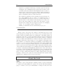
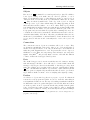
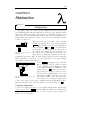
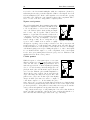
pd-extended build includes extra libraries so you don’t need to install them separately. When you run it you should see a console window that looks something
like Fig. 2.1.
fig 2.1: Pure Data console
Testing Pure Data
The first thing to do is turn on the audio and test it. Start by entering the
Media menu on the top bar and select Audio ON (or either check the compute
audio box in the console window, or press CTRL+/ on the keyboard.) From
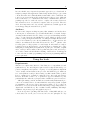
the Media→Test-Audio-and-MIDI menu, turn on the test signal. You should
hear a clear tone through your speakers, quiet when set to -40.0dB and much
louder when set to -20.0dB . When you are satisfied that Pure Data is making
sound close the test window and continue reading. If you don’t hear a sound
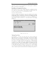
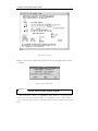
you may need to choose the correct audio settings for your machine. The audio
settings summary will look like that shown in Fig. 2.3. Choices available might
be Jack, ASIO, OSS, ALSA or the name of a specific device you have installed
as a sound card. Most times the default settings will work. If you are using
Jack (recommended), then check that Jack audio is running with qjackctl on
2.2 How does Pure Data work?
7
fig 2.2: Test signal
Linux or jack-pilot on MacOSX. Sample rate is automatically taken from the
soundcard.
fig 2.3: Audio settings pane.
SECTION 2.2
How does Pure Data work?
Pure Data uses a kind of programming called dataflow, because the data
flows along connections and through objects which process it. The output of
one process feeds into the input of another and there may be many steps in the
flow.
8
Starting with Pure Data
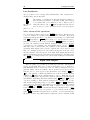
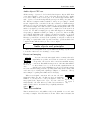
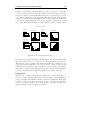
Objects
Here is a box
. A musical box, wound up and ready to play. We call these
boxes objects. Stuff goes in, stuff comes out. For it to pass into, or out of
them, objects must have inlets or outlets. Inlets are at the top of an object box,
outlets are at the bottom. Here is an object that has two inlets and one outlet:
. They are shown by small “tabs” on the edge of the object box. Objects
contain processes or procedures which change the things appearing at their
inlets and then send the results to one or more outlets. Each object performs
some simple function and has a name appearing in its box that identifies what
it does. There are two kinds of object, intrinsics which are part of the core
Pd program, and externals which are separate files containing add-ons to the
core functions. Collections of externals are called libraries and can be added to
extend the functionality of Pd. Most of the time you will neither know nor care
whether an object is intrinsic or external. In this book and elsewhere the words
process, function and unit are all occasionally used to refer to the object boxes
in Pd.
Connections
The connections between objects are sometimes called cords or wires. They
are drawn in a straight line between the outlet of one object and the inlet of
another. It is okay for them to cross, but you should try to avoid this since it
makes the patch diagram harder to read. At present there are two degrees of
thickness for cords. Thin ones carry message data and fatter ones carry audio
signals. Max/MSP TM and probably future versions of Pd will offer different
colours to indicate the data types carried by wires.
Data
The “stuff” being processed comes in several flavours, video frames, sound signals and messages. In this book we will only be concerned with sounds and
messages. Objects give clues about what kind of data they process by their
name. For example, an object that adds together two sound signals looks like
+~ . The + means this is an addition object, and the ∼ (tilde character) means
it object operates on signals. Objects without the tilde are used to process messages, which we shall concentrate on before studying audio signal processing.
Patches
A collection of objects wired together is a program or patch. For historical
reasons the words program and patch2 are used to mean the same thing in
sound synthesis. Patches are an older way of describing a synthesiser built from
modular units connected together with patch cords. Because inlets and outlets
are at the top and bottom of objects the data flow is generally down the patch.
Some objects have more than one inlet or more than one outlet, so signals and
messages can be a function of many others and may in turn generate multiple
2 A different meaning of patch to the one programmers use to describe changes made to a
program to removes bugs
2.2 How does Pure Data work?
9
new data streams. To construct a program we place processing objects onto an
empty area called a canvas, then connect them together with wires representing
pathways for data to flow along. On each step of a Pure Data program any
new input data is fed into objects, triggering them to compute a result. This
result is fed into the next connected object and so on until the entire chain of
objects, starting with the first and ending with the last have all been computed.
The program then proceeds to the next step, which is to do the same thing all
over again, forever. Each object maintains a state which persists throughout
the execution of the program but may change on each step. Message processing
objects sit idle until they receive some data rather than constantly processing an
empty stream, so we say Pure Data is an event driven system. Audio processing
objects are always running, unless you explicitly tell them to switch off.
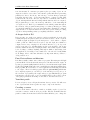
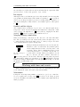
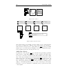
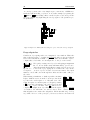
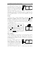
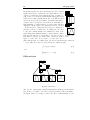
A deeper look at Pd
Before moving on to make some patches consider a quick aside about how Pd
actually interprets its patches and how it works in a wider context. A patch,
or dataflow graph, is navigated by the interpreter to decide when to compute
certain operations. This traversal is right to left and depth first, which is a
computer science way of saying it looks a ahead and tries to go as deep as it
can before moving on to anything higher and moves from right to left at any
branches. This is another way of saying it wants to know what depends on what
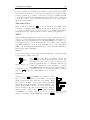
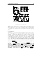
before deciding to calculate anything. Although we think of data flowing down
the graph the nodes in Fig. 2.4 are numbered to show how Pd really thinks
about things. Most of the time this isn’t very important unless you have to
debug a subtle error.
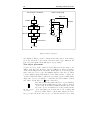
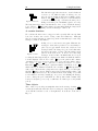
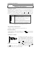
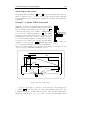
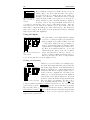
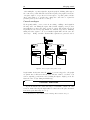
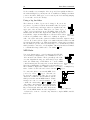
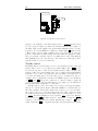
Pure Data software architecture
Pure Data actually consists of more than one program. The main part called pd
performs all the real work and is the interpreter, scheduler and audio engine. A
separate program is usually launched whenever you start the main engine which
is called the pd-gui. This is the part you will interact with when building Pure
Data programs. It creates files to be read by pd and automatically passes them
to the engine. There is a third program called the pd-watchdog which runs
as a completely separate process. The job of the watchdog is to keep an eye on
the execution of programs by the engine and try to gracefully halt the program
if it runs into serious trouble or exceeds available CPU resources. The context
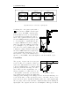
of the pd program is shown in Fig. 2.5 in terms of other files and devices.
Your first patch
Let’s now begin to create a Pd patch as an introductory exercise. We will create
some objects and wire them together as a way to explore the interface.
Creating a canvas
A canvas is the name for the sheet or window on which you place objects. You
can resize a canvas to make it as big as you like. When it is smaller than the
patch it contains, horizontal and vertical scrollbars will allow you to change the
10
Starting with Pure Data
How we humans look at dataflow
How Pd looks at the graph
x
Right to left
10
Distribute
10
t
7
10
Add one
+1
2
5 * 5
Divide by four
/4
55
100
11
100
*5
3 pow 2
+ 1
Squared
^2
11
Times five
6
10
/ 4
25
55
4
25
Depth first
trigger f f
1
+
Add both branches
+
80
80
x2
+ 5(x+1)
4
fig 2.4: Dataflow computation
area displayed. When you save a canvas its size and position on the desktop
are stored. From the console menu select File→New or type CTRL+n at the
keyboard. A new blank canvas will appear on your desktop.
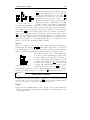
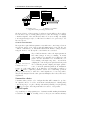
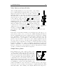
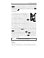
New object placement
To place an object on the canvas select Put→Object from the menu or use
CTRL+1 on the keyboard. An active, dotted box will appear. Move it somewhere
on the canvas using the mouse and click to fix it in place. You can now type the
name of the new object, so type the multiply character * into the box. When
you have finished typing click anywhere on the blank canvas to complete the
operation. When Pure Data recognises the object name you give, it immediately
changes the object box boundary to a solid line and adds a number of inlets
and outlets. You should see a * on the canvas now.
Pure Data searches the paths it knows for objects, which includes the current working directory. If it doesn’t recognise an
+
object because it can’t find a definition anywhere the boundary of the object box remains dotted. Try creating another
fig 2.6: Objects
object and typing some nonsense into it, the boundary will
on a canvas
stay dotted and no inlets or outlets will be assigned. To delete
the object place the mouse cursor close to it, click and hold in order to draw
*
2.2 How does Pure Data work?
11
pd−watchdog
pd (main engine)
Filesystem
pd−gui
Devices
Input/Output
remote machine
OSC
sound.wav
display
MIDI keyboard
UDP/TCP network
intrinsic objects
keyboard
fader box
MIDI
abstraction.pd
mouse
Wii controller
USB ports
patch−file.pd
joystick
parallel ports
external objects
microphone/line
serial ports
textfile.txt
loudspeakers
audio I/O
source.c
Interface
C compiler
fig 2.5: Pure Data software architecture
a selection box around it, then hit delete on the keyboard. Create another
object beneath the last one with an addition symbol so your canvas looks like
Fig. 2.6
Edit mode and wiring
When you create a new object from the menu Pd automatically enters edit
mode, so if you just completed the instructions above you should currently be
in edit mode. In this mode you can make connections between objects, or delete
objects and connections.
Hovering over an outlet will change the mouse cursor to a
new “wiring tool”. If you click and hold the mouse when
+
the tool is active you will be able to drag a connection away
from the object. Hovering over a compatible inlet while in
this state will allow you to release the mouse and make a new
fig 2.7: Wiring
connection. Connect together the two objects you made so
objects
that your canvas looks like Fig. 2.7. If you want to delete a
connection it’s easy, click on the connection to select it and then hit the delete
key. When in edit mode you can move any object to another place by clicking
over it and dragging with the mouse. Any connections already made to the
object will follow along. You can pick up and move more than one object if you
draw a selection box around them first.
*
Initial parameters
Most objects can take some initial parameters or arguments, but these aren’t
always required. They can be created without any if you are going to pass data
via the inlets as the patch is running. The + object can be written as + 3 to
12
Starting with Pure Data
create an object which always adds 3 to its input. Uninitialised values generally
resort to zero so the default behaviour of + would be to add 0 to its input,
which is the same as doing nothing. Contrast this to the default behaviour of
*
which always gives zero.
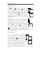
Modifying objects
You can also change the contents of any object box to alter the name and
function, or to add parameters.
In Fig. 2.8 the objects have been changed to give them initial
parameters. The multiply object is given a parameter of 5,
+ 3
which means it multiplies its input by 5 no matter what comes
in. If the input is 4 then the output will be 20. To change the
contents of an object click on the middle of the box where the
fig 2.8: Changing objects
name is and type the new text. Alternatively click once, and
then again at the end of the text to append new stuff, such
as adding 5 and 3 to the objects shown in Fig. 2.8
* 5
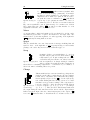
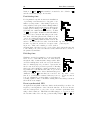
Number input and output
10
* 5
+ 3
53
fig 2.9: Number
boxes
One of the easiest ways to create and view numerical data
is to use number boxes. These can act as input devices to
generate numbers, or as displays to show you the data on a
wire. Create one by choosing Put→Number from the canvas
menu, or use CTRL+3, and place it above the * object. Wire
it to the left inlet. Place another below the + object and
wire the object outlet to the top of the number box as shown
in Fig. 2.9.
Toggling edit mode
Pressing CTRL+E on the keyboard will also enter edit mode. This key combination toggles modes, so hitting CTRL+E again exits edit mode. Exit edit mode
now by hitting CTRL+E or selecting Edit→Edit mode from the canvas menu.
The mouse cursor will change and you will no longer be able to move or modify
object boxes. However, in this mode you can operate the patch components
such as buttons and sliders normally. Place the mouse in the top number box,
click and hold and move it upwards. This input number value will change, and
it will send messages to the objects below it. You will see the second number
box change too as the patch computes the equation y = 5x + 3. To re-enter edit
mode hit CTRL+E again or place a new object.
More edit operations
Other familiar editing operations are available while in edit mode. You can cut
or copy objects to a buffer or paste them back into the canvas, or to another
canvas opened with the same instance of Pd. Take care with pasting objects
in the buffer because they will appear directly on top of the last object copied.
To select a group of objects you can drag a box around them with the mouse.
2.3 Message data and GUI boxes
13
Holding SHIFT while selecting allows multiple separate objects to be added to
the buffer.
•
•
•
•
•
•
CTRL+A
CTRL+D
CTRL+C
CTRL+V
CTRL+X
SHIFT
Select all objects on canvas.
Duplicate the selection.
Copy the selection.
Paste the selection.
Cut the selection.
Select multiple objects.
Duplicating a group of objects will also duplicate any connections between them.
You may modify an object once created and wired up without having it disconnect so long as the new one is compatible the existing inlets and outlets, for
example replacing + with - . Clicking on the object text will allow you
to retype the name and, if valid, the old object is deleted and its replacement
remains connected as before.
Patch files
Pd files are regular text files in which patches are stored. Their names always
end with a .pd file extension. Each consists of a netlist which is a collection of
object definitions and connections between them. The file format is terse and
difficult to understand, which is why we use the GUI for editing. Often there
is a one to one correspondence between a patch, a single canvas, and a file, but
you can work using multiple files if you like because all canvases opened by the
same instance of Pd can communicate via global variables or through send and
receive
objects. Patch files shouldn’t really be modified in a text editor unless
you are an expert Pure Data user, though a plaintext format is useful because
you can do things like search for and replace all occurrences of an object. To
save the current canvas into a file select File→Save from the menu or use the
keyboard shortcut CTRL+s. If you have not saved the file previously a dialogue
panel will open to let you choose a location and file name. This would be a good
time to create a folder for your Pd patches somewhere convenient. Loading a
patch, as you would expect, is achieved with File→Open or CTRL+o.
SECTION 2.3
Message data and GUI boxes
We will briefly tour the basic data types that Pd uses along with GUI objects
that can display or generate that data for us. The message data itself should
not be confused with the objects that can be used to display or input it, so
we distinguish messages from boxes. A message is an event, or a piece of
data that gets sent between two objects. It is invisible as it travels down the
wires, unless we print it or view it in some other way like with the number boxes
above. A message can be very short, only one number or character, or very long,
perhaps holding an entire musical score or synthesiser parameter set. They can
be floating point numbers, lists, symbols, or pointers which are references to
other types like datastructures. Messages happen in logical time, which means
14
Starting with Pure Data
that they aren’t synchronised to any real timebase. Pd processes them as fast
as it can, so when you change the input number box, the output number box
changes instantly. Let’s look at some other message types we’ll encounter while
building patches to create sound. All GUI objects can be placed on a canvas
using the Put menu or using keyboard shortcuts CTRL+1 through CTRL+8, and
all have properties which you can access by clicking them while in edit mode
and selecting the properties pop-up menu item. Properties include things like
colour, ranges, labels and size and are set per instance.
Selectors
With the exception of a bang message, all other message types carry an invisible
selector, which is a symbol at the head of the message. This describes the “type”
of the remaining message, whether it represents a symbol, number, pointer or
list. Object boxes and GUI components are only able to handle appropriate
messages. When a message arrives at an inlet the object looks at the selector
and searches to see if it knows of an appropriate method to deal with it. An
error results when an incompatible data type arrives at an inlet, so for example,
if you supply a symbol type message to a delay object it will complain. . .
error: delay: no method for ’symbol’
Bang message
This is the most fundamental, and smallest message. It just means “compute
something”. Bangs cause most objects to output their current value or advance
to their next state. Other messages have an implicit bang so they don’t need to
be followed with a bang to make them work. A bang has no value, it is just a
bang.
Bang box
A bang box looks like this,
and sends and receives a bang message. It briefly
changes colour, like this , whenever it is clicked or upon receipt of a bang
message to show you one has been sent or received. These may be used as
buttons to initiate actions or as indicators to show events.
Float messages
Floats are another name for numbers. As well as regular (integer) numbers like
1, 2, 3 and negative numbers like −10 we need numbers with decimal points like
−198753.2 or 10.576 to accurately represent numerical data. These are called
floating point numbers, because of the way computers represent the decimal
point position. If you understand some computer science then it’s worth noting
that there are no integers in Pd, everything is a float, even if it appears to be
an integer, so 1 is really 1.0000000. Current versions of Pd use a 32 bit float
representation, so they are between −8388608 and 8388608.
Number box
For float numbers we have already met the number box, which is a dual purpose
GUI element. Its function is to either display a number, or allow you to input
2.3 Message data and GUI boxes
15
one. A bevelled top right corner like this 0
denotes that this object is a
number box. Numbers received on the inlet are displayed and passed directly to
the outlet. To input a number click and hold the mouse over the value field and
move the mouse up or down. You can also type in numbers. Click on a number
box, type the number and hit RETURN. Number boxes are a compact replacement
for faders. By default it will display up to five digits including a sign if negative,
-9999 to 99999, but you can change this by editing its properties. Holding SHIFT
while moving the mouse allows a finer degree of control. It is also possible to
set an upper and lower limit from the properties dialog.
Toggle box
Another object that works with floats is a toggle box. Like a checkbox on any
standard GUI or web form, this has only two states, on or off. When clicked
and it sends out a number 1, clicking again
a cross appears in the box like
causes it to send out a number 0 and removes the cross so it looks like this .
It also has an inlet which sets the value, so it can be used to display a binary
state. Sending a bang to the inlet of a toggle box does not cause the current
value to be output, instead it flips the toggle to the opposite state and outputs
this value. Editing properties also allows you to send numbers other than 1
for the active state.
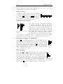
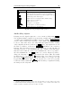
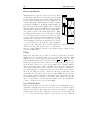
Sliders and other numerical GUI elements
GUI elements for horizontal and vertical sliders can be used as input and display
elements. Their default range is 0 to 127, nice for MIDI controllers, but like
all other GUI objects this can be changed in their properties window. Unlike
those found in some other GUI systems, Pd sliders do not have a step value.
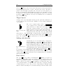
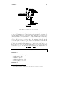
Shown in Fig. 2.10 are some GUI objects at their standard sizes. They can be
A
C
B
D
E
>+12
+6
+2
-0dB
-2
-6
-12
-20
-30
-50
<-99
fig 2.10: GUI Objects A: Horizontal slider B: Horizontal radio box C: Vertical radio box D:
Vertical slider E: VU meter
ornamented with labels or created in any colour. Resizing the slider to make it
bigger will increase the step resolution. A radio box provides a set of mutually
exclusive buttons which output a number starting at zero. Again, they work
equally well as indicators or input elements. A better way to visually display
an audio level is to use a VU meter. This is set up to indicate decibels, so has a
rather strange scale from −99.0 to +12.0. Audio signals that range from −1.0
16
Starting with Pure Data
to +1.0 must first be scaled using the appropriate object. The VU is one of the
few GUI elements that only acts as a display.
General messages
Floats and bangs are types of message, but messages can be more general. Other
message types can be created by prepending a selector that gives them special
meanings. For example, to construct lists we can prepend a list selector to a
set of other types.
Message box
These are visual containers for user definable messages. They can be used to
input or store a message. The right edge of a message box is curved inwards
like this
, and it always has only one inlet and one outlet. They behave
as GUI elements, so when you click a message box it sends its contents to the
outlet. This action can also be triggered if the message box receives a bang
message on its inlet. Message boxes do some clever thinking for us. If we store
something like 5.0 it knows that is a float and outputs a float type, but if we
create a message with text then it will send out a list of symbols, so it is type aware
which saves us having to say things like “float 1.0” as we would in C programs.
It can also abbreviate floating point numbers like 1.0 to 1, which saves time
when inputting integer values, but it knows that they are really floats.
Symbolic messages
A symbol generally is a word or some text. A symbol can represent anything, it
is the most basic textural message in Pure Data. Technically a symbol in Pd can
contain any printable or non-printable character. But most of the time you will
only encounter symbols made out of letters, numbers and some interpunctuation
characters like dash, dot or underscore. The Pd editor does some automatic
conversions: words that can also be interpreted as a number (like 3.141 or 1e +
20) are converted to a float internally (but +20 still is a symbol!). Whitespace
is used by the editor to separate symbols from each other, so you cannot type
a symbol including a space character into a message box. To generate symbols
with backslash-escaped whitespace or other special characters inside use the
makefilename
symbol maker object. The openpanel file dialog object preserves and
escapes spaces and other special characters in filenames, too. Valid symbols are
badger, sound 2, or all your base but not hello there (which is two symbols), or
20 (which will be interpreted as a float, 20.0).
Symbol box
For displaying or inputting text you may use a symbol
box. Click on the display
field and type any text that is a valid symbol and then hit ENTER/RETURN. This
will send a symbol message to the outlet of the box. Likewise, if a symbol
message is received at the inlet it will be displayed as text. Sending a bang
message to a symbol box makes it output any symbol it already contains.
2.3 Message data and GUI boxes
17
Lists
A list is an ordered collection of any things, floats, symbols or pointers that
are treated as one. Lists of floats might be used for building melody sequences
or setting the time values for an envelope generator. Lists of symbols can be
used to represent text data from a file or keyboard input. Most of the time
we will be interested in lists of numbers. A list like {2 127 3.14159 12 } has
four elements, the first element is 2.0 and the last is 12.0. Internally, Pure Data
recognises a list because it has a list selector at the start, so it treats all following
parts of the message as ordered list elements. When a list is sent as a message
all its elements are sent at once. A list selector is attached to the beginning
of the message to determine its type. The selector is the word “list”, which
has a special meaning to Pd. Lists may be of mixed types like {5 6 pick up
sticks }, which has two floats and three symbols. When a list message contains
only one item which is a float it is automatically changed (cast) back to a float.
Lists can be created in several ways, by using a message box, or by using pack ,
which we will meet later, to pack data elements into a list.
Pointers
As in other programming languages, a pointer is the address of some other
piece of data. We can use them to build more complex datastructures, such as
a pointer to a list of pointers to lists of floats and symbols. Special objects exist
for creating and dereferencing pointers, but since they are an advanced topic we
will not explore them further in this book.
Tables, arrays and graphs
A table is sometimes used interchangeably with an array to mean a two dimensional data structure. An array is one of the few invisible objects. Once
declared it just exists in memory. To see it, a separate graph like that shown in
Fig. 2.11 allows us to view its contents.
Graphs have the wonderful property that they are
also GUI elements. You can draw data directly into a
graph using the mouse and it will modify the array it is
attached to. You can see a graph of array1 in Fig. 2.11
that has been drawn by hand. Similarly, if the data in
an array changes and it’s attached to a visible graph
then the graph will show the data as it updates. This
fig 2.11: An array.
is perfect for drawing detailed envelopes or making an
oscilloscope display of rapidly changing signals.
array1
18
Starting with Pure Data
To create a new array select Put→Array from the
menu and complete the dialog box to set up its
name, size and display characteristics. On the canvas a graph will appear showing an array with all
its values initialised to zero. The Y-axis range is
−1.0 to +1.0 by default, so the data line will be in
the centre. If the save contents box is checked
then the array data will be saved along with the
patch file. Be aware that long sound files stored
in arrays will make large patch files when saved
this way. Three draw styles are available, points,
polygon and Bezier to show the data with varying
fig 2.12: Create array.
degrees of smoothing. It is possible to use the same
graph to display more than one array, which is very useful when you wish to see
the relationship between two or more sets of data. To get this behaviour use
the in last graph option when creating an array.
Data is written into or read from a table by an
index number which refers to a position within
a1
it. The index is a whole number. To read and
write arrays several kinds of accessor object are
available. The tabread and tabwrite objects allow you to communicate with arrays using messages. Later we will meet tabread4~ and tabwrite~
objects that can read and write audio signals.
24
The array a1 shown in Fig. 2.13 is written to by
tabread a1
the tabwrite object above it, which specifies the
0.25
target array name as a parameter. The right inlet sets the index and the left one sets the value.
fig 2.13: Accessing an array.
Below it a tabread object takes the index on its
inlet and returns the current value.
0.25
24
tabwrite a1
SECTION 2.4
Getting help with Pure Data
At http://puredata.hurleur.com/ there is an active, friendly forum, and
the mailing list can be subscribed to at [email protected]
Exercises
Exercise 1
On Linux, type pd --help at the console to see the available startup options.
On Windows or MacOSX read the help documentation that comes with your
downloaded distribution.
2.4 Getting help with Pure Data
19
Exercise 2
Use the Help menu, select browse help and read through some built in documentation pages. Be familiar with the control examples and audio examples
sections.
Exercise 3
Visit the online pdwiki at http://puredata.org to look at the enormous range
of objects available in pd-extended.
References
Puckette, M. (1996) “Pure Data: another integrated computer music environment.” Proceedings, Second Intercollege Computer Music Concerts, Tachikawa,
Japan, pp. 37-41.
Puckette, M. (1996) “Pure Data.” Proceedings, International Computer Music
Conference. San Francisco: International Computer Music Association, pp.
269-272.
Puckette, M. (1997) “Pure Data: recent progress.” Proceedings, Third Intercollege Computer Music Festival, Tokyo, Japan, pp. 1-4.
Puckette, M. (2007) “The Theory and Technique of Electronic Music” ISBN
978-981-270-077-3 (World Scientific Press, Singapore)
Zimmer, Frnk. (Editor) (2006) “Bang - A Pure Data Book” ISBN-10 3-93600037-9 (Wolke-Verlag)
Winkler, T. (1998) “Composing Interactive Music, Techniques and Ideas Using
Max” ISBN-10:0-262-23193-X (MIT)
Arduino I/O boards http://www.arduino.cc/
20
Starting with Pure Data
21
CHAPTER 3
Using Pure Data
SECTION 3.1
Basic objects and principles of operation
Now we are familiar with the basics of Pd let’s look at some essential objects
and rules for connecting them together. There are about 20 message objects
you should try to learn by heart because almost everything else is built from
them.
Hot and cold inlets
Most objects operating on messages have a “hot” inlet and (optionally) one or
more “cold” inlets. Messages received at the hot inlet, usually the leftmost one,
will cause computation to happen and output to be generated. Messages on a
cold inlet will update the internal value of an object but not cause it to output
the result yet. This seems strange at first, like a bug. The reason is so that we
can order evaluation. This means waiting for sub-parts of a program to finish
in the right order before proceeding to the next step. From maths you know
that brackets describe the order of a calculation. The result of 4 × 10 − 3 is not
the same as 4 × (10 − 3), we need to calculate the parenthesised parts first. A
Pd program works the same way, you need to wait for the results from certain
parts before moving on.
In Fig. 3.1 a new number box is added to right inlet of * .
This new value represents a constant multiplier k so we can
* 5
compute y = kx + 3. It overrides the 5 given as an initial
+ 3
33
parameter when changed. In Fig. 3.1 it’s set to 3 so we have
y = 3x + 3. Experiment setting it to another value and
fig 3.1: Hot and
then changing the left number box. Notice that changes to
cold inlets
the right number box don’t immediately effect the output,
because it connects to the cold inlet of * , but changes to the left number box
cause the output to change, because it is connected to the hot inlet of * .
10
3
Bad evaluation order
8
8
+
+
16
15
good
bad
fig 3.2: Bad ordering
A problem arises when messages fan out from a single
outlet into other operations. Look at the two patches in
Fig. 3.2. Can you tell the difference? It is impossible
to tell just by looking that one is a working patch and
the other contains a nasty error. Each is an attempt to
double the value of a number by connecting it to both
22
Using Pure Data
sides of a + . When connections are made this way the behaviour is undefined,
but usually happens in the order the connections were made. The first one
works because the right (cold) inlet was connected before the left (hot) one.
In the second patch the arriving number is added to the last number received
because the hot inlet is addressed first. Try making these patches by connecting
the inlets to + in a different order. If you accidentally create errors this way
they are hard to debug.
Trigger objects
A trigger is an object that splits a message up into parts and sends them over
several outlets in order. It solves the evaluation order problem by making the
order explicit.
The order of output is right to left, so a trigger bang float
object outputs a float on the right outlet first, then a
+
bang on the left one. This can be abbreviated as t b f .
20
Proper use of triggers ensures correct operation of units
further down the connection graph. The arguments to a
fig 3.3: Ordering with
trigger may be s for symbol, f for float, b for bang, p
trigger
for pointers and a for any. The “any” type will pass lists
and pointers too. The patch in Fig. 3.3 always works correctly, whatever order
you connect to the + inlets. The float from the right outlet of t f f is always
sent to the cold inlet of + first, and the left one to the hot inlet afterwards.
10
t f f
Making cold inlets hot
An immediate use for our new knowledge of triggers is to
make an arithmetic operator like + respond to either of
+
its inlets immediately. Make the patch shown in Fig. 3.4
7
and try changing the number boxes. When the left one is
changed it sends a float number message to the left (hot)
fig 3.4: Warming an
inlet which updates the output as usual. But now, when
inlet
you change the right number box it is split by t b f into
two messages, a float which is sent to the cold (right) inlet of + , and a bang,
which is sent to the hot inlet immediately afterwards. When it receives a bang
on its hot inlet + computes the sum of the two numbers last seen on its inlets,
which gives the right result.
4
3
t b f
Float objects
The object f is very common. A shorthand for float , which you can also use
if you like to make things clearer, it holds the value of a single floating point
number. You might like to think of it as a variable, a temporary place to store a
number. There are two inlets on f , the rightmost one will set the value of the
object, and the leftmost one will both set the value and/or output it depending
on what message it receives. If it receives a bang message it will just output
whatever value is currently stored, but if the message is a float it will override
3.2 Working with time and events
23
the currently stored value with a new float and immediately output that. This
gives us a way to both set and query the object contents.
Int objects
Although we have noted that integers don’t really exist in Pd, not in a way that
a programmer would understand, whole numbers certainly do. int stores a float
as if it were an integer in that it provides a rounding (truncation) function of
any extra decimal places. Thus 1.6789 becomes 1.0000, equal to 1, when passed
to int .
Symbol and list objects
As for numbers there are likewise object boxes to store lists and symbols in a
temporary location. Both work just like their numerical counterparts. A list
can be given to the right inlet of list and recalled by banging the left inlet.
Similarly symbol can store a single symbol until it is needed.
Merging message connections
When several message connections are all connected to the same inlet that’s
fine. The object will process each of them as they arrive, though it’s up to you
to ensure that they arrive in the right order to do what you expect. Be aware
of race hazards when the sequence is important.
Messages arriving from different sources at the same hot
inlet have no effect on each another, they remain separate
f
and are simply interleaved in the order they arrive, each
11
producing output. But be mindful that where several
connections are made to a cold inlet only the last one
fig 3.5: Messages to
to arrive will be relevant. Each of the number boxes in
same inlet
Fig. 3.5 connects to the same cold inlet of the float box
f
and a bang button to the hot inlet. Whenever the bang button is pressed
the output will be whatever is currently stored in f , which will be the last
number box changed. Which number box was updated last in Fig. 3.5? It was
the middle one with a value of 11.
10
11
12
SECTION 3.2
Working with time and events
With our simple knowledge of objects we can now begin making patches that
work on functions of time, the basis of all sound and music.
Metronome
Perhaps the most important primitive operation is to get a beat or timebase.
To get a regular series of bang events metro provides a clock. Tempo is given
as a period in milliseconds rather than beats per minute (as is usual with most
music programs).
24
Using Pure Data
The left inlet toggles the metronome on and off when it
receives a 1 or 0, while the right one allows you to set
metro 1000
the period. Periods that are fractions of a millisecond are
allowed. The metro emits a bang as soon as it is switched
on and the following bang occurs after the time period.
fig 3.6: Metronome
In Fig. 3.6 the time period is 1000ms, (equal to 1 second).
The bang button here is used as an indicator. As soon as you click the message
box to send 1 to metro it begins sending out bangs which make the bang button
flash once per second, until you send a 0 message to turn it off.
1
0
A counter timebase
We could use the metronome to trigger a sound repeatedly, like a steady drum
beat, but on their own a series of bang events aren’t much use. Although
they are separated in time we cannot keep track of time this way because bang
messages contain no information.
In Fig. 3.7 we see the metronome again. This time the
messages to start and stop it have been conveniently remetro 1000
placed by a toggle switch. I have also added two new
f 0 + 1
messages which can change the period and thus make
24
the metronome faster or slower. The interesting part is
just below the metronome. A float box receives bang
fig 3.7: Counter
messages on its hot inlet. Its initial value is 0 so upon
receiving the first bang message it outputs a float number 0 which the number
box then displays. Were it not for the + 1 object the patch would continue
outputting 0 once per beat forever. However, look closely at the wiring of these
two objects, f and + 1 are connected to form an incrementor or counter.
Each time f recieves a bang it ouputs the number currently stored to + 1
which adds 1 to it. This is fed back into the cold inlet of f which updates its
value, now 1. The next time a bang arrives 1 is output, which goes round again,
through + 1 and becomes 2. This repeats as long as bang messages arrive, each
time the output increases by 1. If you start the metronome in Fig. 3.7 you will
see the number box slowly counting up, once per second. Clicking the message
boxes to change the period will make it count up faster with a 500ms delay
between beats (twice per second), or still faster at 4 times per second (250ms
period).
500
250
Time objects
Three related objects help us manipulate time in the message domain. timer
accurately measures the interval between receiving two bang messages, the first
on its left inlet and the second on its right inlet. It is shown on the left of
Fig. 3.8.
3.3 Data flow control
25
Clicking the first bang button will reset and start
timer
and then hitting the second one will out2000
put the time elapsed (in ms). Notice that timer
250
0
is unusual, it’s one of the few objects where the
timer
delay 1000
pipe 300
delay
right inlet behaves as the hot control.
214.6
0
shown in the middle of Fig. 3.8 will output a
single bang message a certain time period after
fig 3.8: Time objects
receiving a bang on its left inlet. This interval
is set by its first argument or right inlet, or by the value of a float arriving at its
left inlet, so there are three ways of setting the time delay. If a new bang arrives
any pending one is cancelled and a new delay is initiated. If a stop message
arrives then delay is reset and all pending events are cancelled. Sometimes we
want to delay a stream of number messages by a fixed amount, which is where
pipe
comes in. This allocates a memory buffer that moves messages from its
inlet to its outlet, taking a time set by its first argument or second inlet. If you
change the top number box of the right patch in Fig. 3.8 you will see the lower
number box follow it, but lagging behind by 300ms.
bang
stop
Select
This object outputs a bang on one of its outlets matching something in its
argument list. For example select 2 4 6 will output a bang on its second outlet if
it receives a number 4, or on its third outlet when a number 6 arrives. Messages
that do not match any argument are passed through to the rightmost outlet.
This makes it rather easy to begin making simple sequences. The patch in Fig. 3.9 cycles around
0
four steps blinking each bang button in turn. It
f 0 + 1
is a metronome running with a 300ms period and
select 0 1 2 3
a counter. On the first step the counter holds 0,
and when this is output to select it sends a bang
to its first outlet which matches 0. As the counter
fig 3.9: Simple sequencer
increments, successive outlets of select produce a
bang, until the fourth one is reached. When this happens a message containing
0 is triggered which feeds into the cold inlet of f resetting the counter to 0.
metro 300
SECTION 3.3
Data flow control
In this section are a few common objects used to control the flow of data
around patches. As you have just seen select can send bang messages along a
choice of connections, so it gives us a kind of selective flow.
Route
Route behaves in a similar fashion to select, only it operates on lists. If the first
element of a list matches an argument the remainder of the list is passed to the
corresponding outlet.
26
Using Pure Data
So, route badger mushroom snake will send 20.0 to its third outlet
vca 5
when it receives the message {snake 20 }. Non matching lists are passed unchanged to the rightmost outlet.
route vcf vco vca
Arguments can be numbers or symbols, but we tend to
20
0
5
use symbols because a combination of route with lists is
fig 3.10: Routing vala great way to give parameters names so we don’t forues
get what they are for. We have a few named values in
Fig. 3.10 for synthesiser controls. Each message box contains a two element
list, a name-value pair. When route encounters one that matches one of its
arguments it sends it to the correct number box.
vcf 20
Moses
A “stream splitter” which sends numbers below a threshold to its left outlet,
and numbers greater than or equal to the threshold to the right outlet. The
threshold is set by the first argument or a value appearing on the right inlet.
moses 20
splits any incoming numbers at 20.0
Spigot
This is a switch that can control any stream of messages including lists and
symbols. A zero on the right inlet of spigot stops any messages on the left inlet
passing to the outlet. Any non-zero number turns the spigot on.
Swap
It might look like a very trivial thing to do, and you
may ask - why not just cross two wires? In fact swap is
swap
really
useful object. It just exchanges the two values
15
20
on its inlets and passes them to its outlets, but it can
take an argument so it always exchanges a number
fig 3.11: Swapping values
with a constant. It’s useful when this constant is 1 as
shown later for calculating complement 1 − x and inverse 1/x of a number, or
where it is 100 for calculating values as a percent.
15
20
Change
This is useful if we have a stream of numbers, perhaps from a
physical controller like a joystick that is polled at regular inf 0 + 1
tervals, but we only want to know values when they change.
/ 2
3
It is frequently seen preceded by int to denoise a jittery sigint
1.5
nal or when dividing timebases. In Fig. 3.12 we see a counter
change
1
that has been stopped after reaching 3. The components be1
low it are designed to divide the timebase in half. That is
fig 3.12: Pass valto say, for a sequence {1, 2, 3, 4, 5, 6 ...} we will get
ues that change
{1, 2, 3 ...}. There should be half as many numbers in
the output during the same time interval. In other words the output changes
half as often as the input. Since the counter has just passed 3 the output of /
is 1.5 and int truncates this to 1. But this is the second time we have seen 1
metro 1000
3.3 Data flow control
27
appear, since the same number was sent when the input was 2. Without using
change
we would get {1, 1, 2, 2, 3, 3 ...} as output.
Send and receive objects
Very useful for when patches get too visually dense,
or when you are working with patches spread across
many canvases. send and receive objects, abbreviated
fig 3.13: Sends
as s and r work as named pairs. Anything that
goes into the send unit is transmitted by an invisible wire and appears immediately on the receiver, so whatever goes into send bob reappears at receive bob .
29
9
s mary
send mungo send midge
69
receive mary r mungo r midge
Matching sends and receives have global names by
29
9
69
default and can exist in different canvases loaded at
the same time. So if the receive objects in Fig. 3.14
fig 3.14: Receives
are in a different patch they will still pick up the
send values from Fig. 3.13. The relationship is one to many, so only one send
can have a particular name but can be picked up by multiple receive objects
with the same name. In the latest versions of Pd the destination is dynamic
and can be changed by a message on the right inlet.
Broadcast messages
As we have just seen there is an “invisible” environment through which messages
may travel as well as through wires. A message box containing a message that
begins with a semicolon is broadcast and Pd will route it to any destination that
matches the first symbol. This way, activating the message box ; foo 20 is the
same as sending a float message with a value of 20 to the object s foo .
Special message destinations
This method can be used to address arrays with special commands, to talk to
GUI elements that have a defined receive symbol or as an alternative way to talk
to receive objects. If you want to change the size of arrays dynamically they
recognise a special resize message. There is also a special destination (which
always exists) called pd which is the audio engine. It can act on broadcast
messages like ; pd dsp 1 to turn on the audio computation from a patch. Some
examples are shown in Fig. 3.15
a1
;
a1 sinesum 64 0.2 0.2
a2
;
a2 resize 128;
a2 sinesum 128 0.1 0.2;
a2 normalize
gain
;
gain 64
64.00
fig 3.15: Special message broadcasts
28
Using Pure Data
Message sequences
Several messages can be stored in the same message-box as a sequence if separated by commas, so 2, 3, 4, 5 is a message-box that will send four values one
after another when clicked or banged. This happens instantly (in logical time).
This is often confusing to beginners when comparing sequences to lists. When
you send the contents of a message box containing a sequence all the elements
are sent in one go, but as separate messages in a stream. Lists on the other
hand, which are not separated by commas, also send all the elements at the
same time, but as a single list message. Lists and sequences can be mixed, so a
message box might contain a sequence of lists.
SECTION 3.4
List objects and operations
Lists can be quite an advanced topic and we could devote an entire chapter
to this subject. Pd has all the capabilities of a full programming language like
LISP, using only list operations, but like that language all the more complex
functions are defined in terms of just a few intrinsic operations and abstractions. The list-abs collection by Frank Barknecht and others is available in
pd-extended. It contains scores of advanced operations like sorting, reversing,
inserting, searching and performing conditional operations on every element of
a list. Here we will look at a handful of very simple objects and leave it as
an exercise to the reader to research the more advanced capabilities of lists for
building sequencers and data analysis tools.
Packing and unpacking lists
The usual way to create and disassemble lists is to use pack and unpack . Arguments
are given to each which are type identifiers, so pack f f f f is an object that will
wrap up four floats given on its inlets into a single list. They should be presented
in right to left order so that the hot inlet is filled last. You can also give float
values directly as arguments of a pack object where you want them to be fixed,
so pack 1 f f 4 is legal, the first and last list elements will be 1 and 4 unless
over-ridden by the inlets, and the two middle ones will be variable.
foo
bar
2
1
pack s s f f
s packed
fig 3.16: List packing
Start by changing the right number in Fig. 3.16,
then the one to its left, then click on the symbol boxes and type a short string before hitting
RETURN. When you enter the last symbol connected
to the hot inlet of pack you will see the data received by Fig. 3.17 appear in the display boxes
after it is unpacked.
3.4 List objects and operations
29
r packed
The unpack s s f f will expect two symbols and two
unpack s s f f
floats and send them to its four outlets. Items are
1
packed and unpacked in the sequence given in the
2
bar
list, but in right to left order. That means the floats
foo
from unpack s s f f will appear first, starting with the
fig 3.17: List unpacking
rightmost one, then the two symbols ending on the
leftmost one. Of course this happens so quickly you
cannot see the ordering, but it makes sense to happen this way so that if you are
unpacking data, changing it and re-packing into a list everything occurs in the
right order. Note that the types of data in the list must match the arguments
of each object. Unless you use the a (any) type Pd will complain if you try to
pack or unpack a mismatched type.
Substitutions
A message box can also act as a template. When
an item in a message box is written $1 it behaves
$3 $1 $2
$1
as an empty slot that assumes the value of the first
unpack f f f
5
element of a given list. Each of the dollar arguments
15
5
10
$1, $2 and so on, are replaced by the corresponding item in the input list. The message box then
fig 3.18: Dollar substitusends the new message with any slots filled in. List
tion.
elements can be substituted in multiple positions as
seen in Fig. 3.18. The list {5 10 15 } becomes {15 5 10 } when put through
the substitution $3 $1 $2 .
5 6 7
pack 5 10 15
Persistence
You will often want to set up a patch so it’s in a certain state when loaded.
It’s possible to tell most GUI objects to output the last value they had when
the patch was saved. You can do this by setting the init checkbox in the
properties panel. But what if the data you want to keep comes from another
source, like an external MIDI fader board? A useful object is loadbang which
generates a bang message as soon as the patch loads.
You can use this in combination with a message
box to initialise some values. The contents of message
set $1 $2 $3
boxes are saved and loaded with the patch. When you
loadbang
need to stop working on a project but have it load the
4 6 8
last state next time around then list data can be saved
pd synthesiser
in the patch with a message box by using the special
set prefix. If a message box receives a list prefixed by
fig 3.19: Persistence using
set it will be filled with the list, but not immediately
messages
ouput it. The arrangement in Fig. 3.19 is used to keep
a 3 element list for pd synthesiser in a message box that will be saved with
the patch, then generate it to initialise the synthesiser again when the patch is
reloaded.
4 6 8
t a a
30
Using Pure Data
List distribution
An object with 2 or more message inlets will distribute a list of parameters to
all inlets using only the first inlet.
9 7
2
fig 3.20: Distribution
The number of elements in the list must match the number of
inlets and their types must be compatible. In Fig. 3.20 a message
box contains a list of two numbers, 9 and 7. When a pair of
values like this are sent to - with its right inlet unconnected
they are spread over the two inlets, in the order they appear,
thus 9 − 7 = 2.
More advanced list operations
To concatenate two lists together we use list append . It takes two lists and creates
a new one with the second list attached to the end of the first. If given an
argument it will append this to every list it receives. It may be worth knowing
that list is an alias for list append . You can choose to type in either in order to
make it clearer what you are doing. Very similar is list prepend which does almost
the same, but returns a new list with the argument or list at the second inlet
concatenated to the beginning. For disassembling lists we can use list split .
This takes a list on its left inlet and a number on the right inlet (or as an
argument) which indicates the position to split the list. It produces two new
lists, one containing elements below the split point appears on the left outlet,
and the remainder of the list appears on the right. If the supplied list is shorter
than the split number then the entire list is passed unchanged to the right outlet.
The list trim object strips off any selector at the start leaving the raw elements.
SECTION 3.5
Input and output
There are plenty of objects in Pd for reading keyboards, mice, system timers,
serial ports and USB. There’s not enough room in this book to do much more
than summarise them, so please refer to the Pd online documentation for your
platform. Many of these are available only as external objects, but several are
built into Pd core. Some depend on the platform used, for example comport and
key
are only available on Linux and MacOS. One of the most useful externals
available is hid which is the “human interface device”. With this you can
connect joysticks, game controllers, dance mats, steering wheels, graphics tablets
and all kinds of fun things. File IO is available using textfile and qlist objects,
objects are available to make database transactions to MySQL, and of course
audio file IO is simple using a range of objects like writesf~ and readsf~ . MIDI files
can be imported and written with similar objects. Network access is available
through netsend and netreceive which offer UDP or TCP services. Open Sound
Control is available using the external OSC library by Martin Peach or dumpOSC
and sendOSC objects. You can even generate or open compressed audio streams
using mp3cast~ and similar externals, and you can run code from other languages
like python and lua. A popular hardware peripheral for use in combination with
3.5 Input and output
31
Pd is the Arduino board which gives a number of buffered analog and digital
lines, serial and parallel, for robotics and control applications. Nearly all of this
is quite beyond the scope of this book. The way you set up your DAW and build
your sound design studio is an individual matter, but Pd should not disappoint
you when it comes to I/O connectivity. We will now look at a few common
input and output channels.
The print object
Where would we be without a print object? Not much use for making sound,
but vital for debugging patches. Message domain data is dumped to the console
so you can see what is going on. You can give it a non-numerical argument
which will prefix any output and make it easier to find in a long printout.
MIDI
When working with musical keyboards there are objects to help integrate these
devices so you can build patches with traditional synthesiser and sampler behaviours. For sound design this is great for attaching MIDI fader boards to control parameters, and of course musical interface devices like breath controllers
and MIDI guitars can be used. Hook up any MIDI source to Pd by activating a
MIDI device from the Media->MIDI menu (you can check this is working from
Media->Test Audio and MIDI).
Notes in
You can create single events to trigger from individual keys, or have layers and
velocity fades by adding extra logic.
The notein object produces note number, velocity and
channel values on its left, middle and right outlets. You
127 velocity
may assign an object to listen to only one channel by giv60 note
ing it an argument from 1 to 15. Remember that note-off
fig 3.21: MIDI note in messages are equivalent to a note-on with zero velocity in
many MIDI implementations and Pd follows this method.
You therefore need to add extra logic before connecting an oscillator or sample
player to notein so that zero valued MIDI notes are not played.
notein
1
channel
Notes out
Another object noteout sends MIDI to external devices. The
first, second and third inlets set note number, velocity and
channel respectively. The channel is 1 by default. Make
sure you have something connected that can play back MIDI
and set the patch shown in Fig. 3.22 running with its toggle
switch. Every 200ms it produces a C on a random octave
with a random velocity value between 0 and 127. Without
further ado these could be sent to noteout , but it would cause
each MIDI note to “hang”, since we never send a note-off
message. To properly construct MIDI notes you need makenote
metro 200
t b b
random 3
random 127
* 12
+ 48
notelength
makenote 984.1
noteout
fig 3.22: MIDI
note generation
32
Using Pure Data
which takes a note-number and velocity, and a duration (in milliseconds) as its
third argument. After the duration has expired it automatically adds a note-off.
If more than one physical MIDI port is enabled then noteout sends channels 1 to
16 to port 1 and channels 17 to 32 to port 2 etc.
Continuous controllers
Two MIDI input/output objects are provided to receive and send continuous
controllers, ctlin and ctlout . Their three connections provide, or let you set, the
controller value, controller number and MIDI channel. They can be instantiated
with arguments, so ctlin 10 1 picks up controller 10 (pan position) on MIDI
channel 1.
MIDI to Frequency
Two numerical conversion utilities are provided to convert between MIDI note
numbers and Hz. To get from MIDI to Hz use mtof . To convert a frequency in
Hz to a MIDI note number use ftom .
Other MIDI objects
For pitchbend, program changes, system exclusive, aftertouch and other MIDI
functions you may use any of the objects summarised in Tbl. 3.23. System
exclusive messages may be sent by hand crafting raw MIDI bytes and outputting
via the midiout object. Most follow the inlet and outlet template of notein and
noteout
having a channel as the last argument, except for midiin and sysexin which
receive omni (all channels) data.
MIDI in object
Object
notein
Get note data
bendin
Get pitchbend
−63 to +64
pgmin
MIDI out object
Function
Object
data
Function
noteout
Send note data.
bendout
Send pitchbend data
−64 to +64.
Get program changes.
pgmout
Send program changes.
ctlin
Get continuous
troller messages.
ctlout
Send continuous controller messages.
touchin
Get channel aftertouch
data.
touchout
Send channel
touch data.
polytouchin
Polyphonic touch data
in
polytouchout
Polyphonic touch output
polytouchin
Send polyphonic aftertouch.
polytouchin
Get polyphonic aftertouch.
midiin
Get unformatted raw
MIDI
midiout
Send raw MIDI to device.
sysexin
Get system exclusive
data
con-
No
output
counterpart
fig 3.23: List of MIDI objects
Use
midiout
after-
object
3.6 Working with numbers
33
SECTION 3.6
Working with numbers
Arithmetic objects
Objects that operate on ordinary numbers to provide basic maths functions are
summarised in Tbl. 3.24 All have hot left and cold right inlets and all take one
argument that initialises the value otherwise received on the right inlet. Note
the difference between arithmetic division with / and the div object. The
modulo operator gives the remainder of dividing the left number by the right.
Object
Function
+
Add two floating point numbers
-
Subtract number on right inlet from number on left inlet
/
Divide lefthand number by number on right inlet
*
Multiply two floating point numbers
div
Integer divide, how many times the number on the right
inlet divides exactly into the number on the left inlet
mod
Modulo, the smallest remainder of dividing the left number into any integer multiple of the right number
fig 3.24: Table of message arithmetic operators
Trigonometric maths objects
A summary of higher maths functions is given in Tbl. 3.25.
Random numbers
A useful ability is to make random numbers. The random object gives integers
over the range given by its argument including zero, so random 10 gives 10 possible
values from 0 to 9.
Arithmetic example
An example is given in Fig. 3.26 to show correct ordering in a patch to calculate the mean
random 100 random 100 random 100
of three random numbers. We don’t have to
96
12
88
make every inlet hot, just ensure that every+
thing arrives in the correct sequence by trig+
/ 3
gering the random objects properly. The first
65.333
random
(on the right) supplies the cold inlet of
+
the
lower
, the middle one to the cold inlet
fig 3.26: Mean of three random
floats
of the upper + . When the final (left) random
is generated it passes to the hot inlet of the
first + , which computes the sum and passes it to the second + hot inlet.
Finally we divide by 3 to get the mean value.
trigger bang bang bang
34
Using Pure Data
Object
Function
cos
The cosine of a number given in radians. Domain: −π/2
to +π/2. Range: −1.0 to +1.0.
sin
tan
atan
atan2
exp
log
abs
sqrt
pow
The sine of a number in radians, domain −π/2 to +
π/2, range −1.0 to +1.0
Tangent of number given in radians. Range: 0.0 to ∞
at ±π/2
Arctangent of any number in domain ±∞ Range: ±π/2
Arctangent of the quotient of two numbers in Cartesian plane. Domain: any floats representing X, Y pair.
Range: angle in radians ±π
Exponential function ex for any number.
to ∞
Range 0.0
Natural log (base e) of any number. Domain:
to ∞. Range: ±∞ (−∞ is −1000.0)
0.0
Absolute value of any number. Domain ±∞. Range 0.0
to ∞
The square root of any positive number.
0.0 to ∞
Domain
Exponentiate the left inlet to the power of the right inlet.
Domain: positive left values only.
fig 3.25: Table of message trigonometric and higher math operators
Comparative objects
In Tbl. 3.27 you can see a summary of comparative objects. Output is either
1 or 0 depending on whether the comparison is true or false. All have hot left
inlets and cold right inlets and can take an argument to initialise the righthand
value.
Object
Function
>
True if the number at the left inlet is greater than the
right inlet.
<
True if the number at the left inlet is less than the right
inlet.
>=
True if the number at the left inlet is greater than or
equal to the right inlet.
<=
True if the number at the left inlet is less than or equal
to the right inlet.
==
True if the number at the left inlet is equal to the right
inlet.
!=
True if the number at the left inlet is not equal to the
right inlet
fig 3.27: List of comparative operators
3.7 Common idioms
35
Boolean logical objects
There are a whole bunch of logical objects in Pd including bitwise operations
that work exactly like C code. Most of them aren’t of much interest to us in this
book, but we will mention the two important ones || and && . The output of
||
, logical OR, is true if either of its inputs are true. The output of && , logical
AND, is true only when both its inputs are true. In Pd any non-zero number is
“true”, so the logical inverter or “not” function is unnecessary because there are
many ways of achieving this using other objects. For example, you can make a
logical inverter by using != with 1 as its argument.
SECTION 3.7
Common idioms
There are design patterns that crop up frequently in all types of programming. Later we will look at abstraction and how to encapsulate code into new
objects so you don’t find yourself writing the same thing again and again. Here
I will introduce a few very common patterns.
Constrained counting
We have already seen how to make a counter by repeatedly incrementing the value stored in a float box. To turn an increasing metro 500
f
+ 1
or decreasing counter into a cycle for repeated sequences there mod 8
is an easier way than resetting the counter when it matches trigger f f f
an upper limit, we wrap the numbers using mod . By inserting mod 4 mod 3
mod
into the feedback path before the increment we can ensure 3
1
7
the counter stays bounded. Further mod units can be added to
3.28:
the number stream to generate polyrhythmic sequences. You fig
Constrained
will frequently see variations on the idiom shown in Fig. 3.28. counter.
This is the way we produce multi-rate timebases for musical
sequencers, rolling objects or machine sounds that have complex repetitive patterns.
Accumulator
A similar construct to a counter is the accumulator or integrator.
This reverses the positions of f and + to create an integrator that
0
stores the sum of all previous number messages sent to it. Such an
fig 3.29: arrangement is useful for turning “up and down” messages from an
Accumuinput controller into a position. Whether to use a counter or acculator.
mulator is a subtle choice. Although you can change the increment
step of the counter by placing a new value on the right inlet of + it will not
take effect until the previous value in f has been used. An accumulator on the
other hand can be made to jump different intervals immediately by the value
sent to it. Note the important difference, an accumulator takes floats as an
input while a counter takes bang messages.
1
-1
+
f
36
Using Pure Data
Rounding
An integer function, int , also abbreviated i gives the
whole part of a floating point number. This is a trun+ 0.5
cation, which just throws away any decimal digits. For
int
i
positive numbers it gives the floor function, written ⌊x⌋
0
1
which is the integer less than or equal to the input value.
But take note of what happens for negative values, applyfig 3.30: Rounding
ing int to −3.4 will give 3.0, an integer greater than or
equal to the input. Truncation is shown on the left of Fig. 3.30. To get a regular rounding for positive numbers, to pick the closest integer, use the method
shown on the right side of Fig. 3.30. This will return 1 for an input of 0.5 or
more and 0 for an input of 0.49999999 or less.
0.99
0.51
Scaling
This is such a common idiom you will see it almost
everywhere. Given a range of values such as 0 to 127
* 0.070866
* $1
we may wish to map this onto another set of values,
inlet offset
the domain, such as 1 to 10. This is the same as
+
$2
+ 1
changing the slope and zero intersect of a line following
outlet
9.999
y = mx + c. To work out the values you first obtain
fig 3.31: Scaling
the bottom value or offset, in this case +1. Then a
multiplier value is needed to scale for the upper value, which given an input of
127 would satisfy 10 = 1 + 127x, so moving the offset we get 9 = 127x, and
dividing by 127 we get x = 9/127 or x = 0.070866. You can make a subpatch
or an abstraction for this as shown in Fig. 6.1, but since only two objects are
used it’s more sensible to do scaling and offset as you need it.
127
inlet value
inlet scale
Looping with until
Unfortunately, because it must be designed
this way, until has the potential to cause
until
a complete system lock-up. Be very care0
ful to understand what you are doing with
f
+ 1
this. A bang message on the left inlet of
sel 256 t f f
until
will set it producing bang messages
swap 129
cheby
as
fast
as the system can handle! These do
not stop until a bang message is received on
/ 128
t f f
the right inlet. Its purpose is to behave as a
*
fast loop construct performing message do* 2
main computation quickly. This way you
- 1
can fill an entire wavetable or calculate a
tabwrite cheby
complex formula in the time it takes to profig 3.32: Using until
cess a single audio block. Always make sure
the right inlet is connected to a valid terminating condition. In Fig. 3.32 you
can see an example that computes the second Chebyshev polynomial according
t b b
3.7 Common idioms
37
to y = 2x2 − 1 for the range −1.0 to +1.0 and fills a 256 step table with the
result. As soon as the bang button is pressed a counter is reset to zero and then
until
begins sending out bangs. These cause the counter to rapidly increment
until select matches 256 whereupon a bang is sent to the right inlet of until
stopping the process. All this will happen in a fraction of a millisecond. Meanwhile we use the counter output to calculate a Chebyshev curve and put it into
the table.
A safer way to use until is shown in Fig. 3.33. If you know in
advance that you want to perform a fixed number of operations
until
then use it like a for loop. In this case you pass a non-zero
float
to the left inlet. There is no terminating condition, it
fig 3.33:
for
256
stops when the specified number of bangs has been sent, 256
bangs in the example shown.
256
min 1
Message complement and inverse
Here is how we obtain the number that is 1 − x for any x.
The complement of x is useful when you want to balance
/
two numbers so they add up to a constant value, such as
0.75
2
in panning. The swap object exchanges its inlet values,
or any left inlet value with its first argument. Therefore,
fig 3.34: Message rewhat happens with the left example of Fig. 3.34 is the
ciprocal and inverse
calculates 1 − x, which for an input of 0.25 gives 0.75.
Similarly the inverse of a float message 1/x can be calculated by replacing the
with a / .
0.25
0.5
swap 1
swap 1
Random selection
To choose one of several events at random a combination of random
and select will generate a bang message on the select outlet corresponding to one of its arguments. With an initial argument of 4
random
produces a range of 4 random integer numbers starting at 0,
so we use select 0 1 2 3 to select amongst them. Each has an equal
probability, so every outlet will be triggered 25% of the time on
average.
metro 500
random 4
select 0 1 2 3
fig
3.35:
Random
select.
Weighted random selection
metro 500
random 100
moses 10
moses 50
fig
3.36:
Weighted
random select.
A simple way to get a bunch of events with a certain probability distribution is to generate uniformly distributed numbers
and stream them with moses . For example moses 10 sends integers
greater than 9.0 to its right outlet. A cascade of moses objects
will distribute them in a ratio over the combined outlets when
the sum of all ratios equals the range of random numbers. The
outlets of moses 10 distribute the numbers in the ratio 1 : 9. When
the right outlet is further split by moses 50 as in Fig. 3.36 numbers
in the range 0.0 to 100.0 are split in the ratio 10 : 40 : 50, and
38
Using Pure Data
since the distribution of input numbers is uniform they are sent to one of three
outlets with 10%, 40% and 50% probability.
Delay cascade
Sometimes we want a quick succession of bangs in a
certain fixed timing pattern. An easy way to do this
is to cascade delay objects. Each delay 100 in Fig. 3.37
adds a delay of 100 milliseconds. Notice the abbrieved form of the object name is used.
del 100
del 100
del 100
del 100
fig 3.37: Delay cascade.
Last float and averages
If you have a stream of float values and want to
keep the previous value to compare to the current
t f b
one then the idiom shown on the left of Fig. 3.38
f
f
will do the job. Notice how a trigger is employed to
2
+
first bang the last value stored in the float box and
/ 2
12.5
then update it with the current value via the right
inlet. This can be turned into a simple “lowpass”
fig 3.38: Last value and avor averaging filter for float messages as shown on
eraging
the right of Fig. 3.38. If you add the previous value
to the current one and divide by two you obtain the average. In the example
shown the values were 10 followed by 15, resulting in (10 + 15)/2 = 12.5.
3
10
t f b
trigger f f
15
Running maximum (or minimum)
Giving max a very small argument and connecting whatever passes
through it back to its right inlet gives us a way to keep track of the
largest value. In Fig. 3.39 the greatest past value in the stream has
been 35. Giving a very large argument to min provides the opposite
behaviour for tracking a lowest value. If you need to reset the maximum or minimum tracker just send a very large or small float value
to the cold inlet to start again.
9
max 1e-21
t f f
35
fig 3.39:
Biggest
so far
Float lowpass
Using only * and + as shown in Fig. 3.40 we can low pass
filter a stream of float values. This is useful to smooth data from
an external controller where values are occasionally anomalous.
It follows the filter equation yn = Axn + Bxn−1 . The strength
of the filter is set by the ratio A : B. Both A and B should be
between 0.0 and 1.0 and add up to 1.0. Note that this method
will not converge on the exact input value, so you might like to
follow it with int if you need numbers rounded to integer values.
38
* 0.1
+
* 0.9
37.26
fig 3.40: Low
pass for floats
39
CHAPTER 4
Pure Data Audio
SECTION 4.1
Audio objects
We have looked at Pd in enough detail now to move on to the next level.
You have a basic grasp of dataflow programming and know how to make patches
that process numbers and symbols. But why has no mention been made of audio
yet? Surely it is the main purpose of our study? The reason for this is that
audio signal processing is a little more complex in Pd than the numbers and
symbols we have so far considered, so I wanted to leave this until now.
Audio connections
I already mentioned that there two kinds of objects and data for messages
and signals. Corresponding to these there are two kinds of connections, audio
connections and message connections. There is no need to do anything special
to make the right kind of connection. When you connect two objects together
Pd will work out what type of outlet you are attempting to connect to what
kind of inlet and create the appropriate connection. If you try to connect an
audio signal to a message inlet, then Pd will not let you, or it will complain
if there is allowable but ambiguous connection. Audio objects always have a
name ending with a tilde (∼) and the connections between them look fatter
than ordinary message connections.
Blocks
The signal data travelling down audio cords is made of samples, single floating
point values in a sequence that forms an audio signal. Samples are grouped
together in blocks.
A block, sometimes also called a vector, typically has 64 samples inside it, but you can
31.4
15.9
26.5
35.8
change this in certain circumstances. ObWire
B
B
B
B
jects operating on signal blocks behave like
97.9
42.3
84.6
26.4
ordinary message objects, they can add, subInlet
tract, delay or store blocks of data, but do
Object Box
+~
so by processing one whole block at a time.
A +B A +B A +B A + B
In Fig. 4.1 streams of blocks are fed to the
129.3 58.2
111.1 62.2
two inlets. Blocks appearing at the outlet
fig 4.1: Object processing data.
have values which are the sum of the corresponding values in the two input blocks.
Because they process signals made of blocks, audio objects do a lot more work
than objects that process messages.
Signal Block
A1
1
2
A2
3
A3
A4
4
1
1
2
2
3
3
4
4
40
Pure Data Audio
Audio object CPU use
All the message objects we looked at in the last chapters only use CPU when
event driven dataflow occurs, so most of the time they sit idle and consume
no resources. Many of the boxes we put on our sound design canvases will be
audio objects, so it’s worth noting that they use up some CPU power just being
idle. Whenever compute audio is switched on they are processing a constant
stream of signal blocks, even if the blocks only contain zeros. Unlike messages
which are processed in logical time, signals are processed synchronously with
the soundcard sample rate. This real-time constraint means glitches will occur
unless every signal object in the patch can be computed before the next block
is sent out. Pd will not simply give up when this happens, it will struggle
along trying to maintain real-time processing, so you need to listen carefully,
as you hit the CPU limit of the computer you may hear crackles or pops. It is
also worth knowing how audio computation relates to messages computation.
Messages operations are executed at the beginning of each pass of audio block
processing, so a patch where audio depends on message operations which don’t
complete in time will also fail to produce correct output.
SECTION 4.2
Audio objects and principles
There are a few ways that audio objects differ from message objects so let’s
look at those rules now before starting to create sounds.
Fanout and merging
You can connect the same signal outlet to as many other audio
signal inlets as you like, and blocks are sent in an order which
wrap~
*~ -1
corresponds to the creation of the connections, much like message
fig 4.2: Sigconnections. But unlike messages, most of the time this will have
nal fanout is
no effect whatsoever, so you can treat audio signals that fan out
Okay.
as if they were perfect simultaneous copies. Very seldom you may
meet rare and interesting problems, especially with delays and feedback, that
can be fixed by reordering audio signals (see Chapter 7 of Puckette, “Theory
and technique” regarding time shifts and block delays).
phasor~ 440
When several signal connections all come into the same
signal inlet that’s also fine. In this case they are implicitly
summed, so you may need to scale your signal to reduce its
range again at the output of the object. You can connect as
many signals to the same inlet as you like, but sometimes it
makes a patch easier to understand if you explicitly sum them
with a +~ unit.
osc~ 120
osc~ 240
*~ 0.5
fig 4.3: Merging signals is
Okay.
Time and resolution
Time is measured in seconds, milliseconds (one thousandth of a second, written 1ms) or samples. Most Pd times are in ms. Where time is measured in
4.2 Audio objects and principles
41
samples this depends on the sampling rate of the program or the sound card of
the computer system on which it runs. The current sample rate is returned by
the samplerate~ object. Typically a sample is 1/44100th of a second and is the
smallest unit of time that can be measured as a signal. But the time resolution
also depends on the object doing the computation. For example metro and vline~
are able to deal in fractions of a millisecond, even less than one sample. Timing irregularities can occur where some objects are only accurate to one block
boundary and some are not.
Audio signal block to messages
To see the contents of a signal block we can take a snapshot or an average. The
env~
object provides the RMS value of one block of audio data scaled 0 to 100
in dB, while snapshot~ gives the instantaneous value of the last sample in the
previous block. To view an entire block for debugging print~ can be used. It
accepts an audio signal and a bang message on the same inlet and prints the
current audio block contents when banged.
Sending and receiving audio signals
Audio equivalents of send and receive are written send~ and receive~ , with
shortened forms s~ and r~ . Unlike message sends only one audio send can
exist with a given name. If you want to create a signal bus with many to one
connectivity use throw~ and catch~ instead. Within subpatches and abstractions
we use the signal objects inlet~ and outlet~ to create inlets and outlets.
Audio generators
Only a few objects are signal sources. The most important and simple one is
the phasor~ . This outputs an asymmetrical periodic ramp wave and is used at
the heart of many other digital oscillators we are going to make. Its left inlet
specifies the frequency in Hz, and its right inlet sets the phase, between 0.0 and
1.0. The first and only argument is for frequency, so a typical instance of a
phasor looks like phasor~ 110 . For sinusoidal waveforms we can use osc~ . Again,
frequency and phase are set by the left and right inlets, or frequency is set by
the creation parameter. A sinusoidal oscillator at concert A pitch is defined by
osc~ 440
. White noise is another commonly used source in sound design. The
noise generator in Pd is simply noise~ and has no creation arguments. Its output
is in the range −1.0 to 1.0. Looped waveforms stored in an array can be used
to implement wavetable synthesis using the tabosc4~ object. This is a 4 point
interpolating table ocillator and requires an array that is a power of 2, plus 3
(eg. 0 to 258) in order to work properly. It can be instantiated like phasor~ or
osc~
with a frequency argument. A table oscillator running at 3kHz is shown in
Fig. 4.4. It takes the waveform stored in array A and loops around this at the
frequency given by its argument or left inlet value. To make sound samplers
we need to read and write audio data from an array. The index to tabread~ and
its interpolating friend tabread4~ is a sample number, so you need to supply a
signal with the correct slope and magnitude to get the proper playback rate.
You can use the special set message to reassign tabread4~ to read from another
42
Pure Data Audio
phasor~ 3000
A
B
*~ 64
tabread~ A
tabsend~ B
*~ 0.1
dac~
fig 4.4: Table oscillator
;
snum set kit1-01;
phase 1, 4.41e+08 1e+07;
;
snum set kit1-02;
phase 1, 4.41e+08 1e+07;
;
snum set kit1-03;
phase 1, 4.41e+08 1e+07;
;
snum set kit1-04;
phase 1, 4.41e+08 1e+07;
kit1-01
kit1-02
kit1-03
kit1-04
r snum r phase
vline~
loadbang
tabread4~
hip~ 5
read ./sounds/ttsnr.wav kit1-01, read ./sounds/jrsnr.wav
kit1-02, read ./sounds/dlsnr.wav kit1-03, read
./sounds/ezsnr.wav kit1-04
*~ 0.5
soundfiler
dac~
fig 4.5: Sample replay from arrays
array. The message boxes in Fig. 4.5 allow a single object to play back from
more than one sample table. First the target array is given via a message to
snum, and then a message is sent to phase which sets vline~ moving up at 44100
samples per second. The arrays are initially loaded, using a multi-part message,
from a sounds folder in the current patch directory.
Audio line objects
For signal rate control data the line~ object is useful. It is generally programmed
with a sequence of lists. Each list consists of a pair of numbers, the first being a
level to move to and the second number is the time in milliseconds to take getting
there. The range is usually between 1.0 and 0.0 when used as an audio control
signal, but it can be any value such as when using line~ to index a table. A
more versatile line object is called vline~ , which we will meet in much more detail
later. Amongst its advantages are very accurate sub-millisecond timing and the
ability to read multi-segment lists in one go and to delay stages of movement.
Both these objects are essential for constructing envelope generators and other
control signals.
4.2 Audio objects and principles
43
Audio input and output
Audio IO is achieved with the adc~ and dac~ objects. By default these offer two
inlets or outlets for stereo operation, but you can request as many additional
sound channels as your sound system will handle by giving them numerical
arguments.
Example: A simple MIDI monosynth
notein
Using the objects we’ve just discussed let’s create a little
MIDI keyboard controlled music synthesiser as shown in stripnote
mtof
Fig. 4.6. Numbers appearing at the left outlet of notein
control the frequency of an oscillator. MIDI numbers t f b
0, 1 10 0, 0 100 20
are converted to a Hertz frequency by mtof . The MIDI
osc~ vline~ / 127
standard, or rather general adherence to it, is a bit woolly
*~
by allowing note-off to also be a note-on with a velocity of *~
zero. Pd follows this definition, so when a key is released dac~
it produces a note with a zero velocity. For this simple
example we remove it with stripnote , which only passes fig 4.6: MIDI note
control
note-on messages when their velocity is greater than zero.
The velocity value, ranging between 1 and 127 is scaled to between 0 and 1 in
order to provide a rudimentary amplitude control.
20ms
100ms
10ms
Level
10ms
so really start
at zero
Time
after a 0 millisecond delay
return to zero
in 10 milliseconds
move to 1
start at zero
taking 100 milliseconds
0, 1 10 0, 0 100 20
after a 20 millisecond delay
vline~
fig 4.7: Anatomy of vline message
So, here’s a great place to elaborate on the anatomy of the message used
to control vline~ as shown in Fig. 4.7. The syntax makes perfect sense, but
sometimes it’s hard to visualise without practice. The general form has three
numbers per list. It says: “go to some value”, given by the first number, then
44
Pure Data Audio
“take a certain time to get there”, which is the second number in each list. The
last number in the list is a time to wait before executing the command, so it
adds an extra wait for a time before doing it”. What makes vline~ cool is you
can send a sequence of list messages in any order, and so long as they make
temporal sense then vline~ will execute them all. This means you can make
very complex control envelopes. Any missing arguments in a list are dropped
in right to left order, so a valid exception is seen in the first element of Fig. 4.7
where a single 0 means “jump immediately to zero” (don’t bother to wait or
take any time getting there).
Audio filter objects
Six or seven filters are used in this book. We will not look at them in much
detail until we need to because there is a lot to say about their usage in each
case. Simple one pole and one zero real filters are given by rpole~ and rzero~ .
Complex one pole and one zero filters are cpole~ and czero~ . A static biquad
filter biquad~ also comes with a selection of helper objects to calculate coefficients
for common configurations and lop~ , hip~ , and bp~ 1 provide the standard low,
high and bandpass responses. These are easy to use and allow message rate
control of their cutoff frequencies and, in the case of bandpass, resonance. The
first and only argument of the low and high pass filters is frequency, so typical
instances may look like lop~ 500 and hip~ 500 . Bandpass takes a second parameter
for resonance like this bp~ 100 3 . Fast signal rate control of cutoff is possible using
the versatile vcf~ “voltage controlled filter”. Its first argument is cutoff frequency
and its second argument is resonance, so you might use it like vcf~ 100 2 . With
high resonances this provides a sharp filter that can give narrow bands. An
even more colourful filter for use in music synthesiser designs is available as an
external called moog~ , which provides a classic design that can self oscillate.
Audio arithmetic objects
Audio signal objects for simple arithmetic are summarised in Tbl. 4.8.
Object
+~
Function
Add two signals (either input will also accept a message)
-~
Subtract righthand signal from lefthand signal
/~
Divide lefthand signal by right signal
*~
Signal multiplication
wrap~
Signal wrap, constrain any signal between 0.0 and 1.0
fig 4.8: List of arithmetic operators
Trigonometric and math objects
A summary of higher maths functions is given in Tbl. 4.9. Some signal units
are abstractions defined in terms of more elementary intrinsic objects and those
marked * are only available through external libraries in some Pd versions.
4.2 Audio objects and principles
Object
Function
cos~
Signal version of cosine function. Domain: −1.0 to +
1.0. Note the input domain is “rotation normalised”
sin~
Not intrinsic but defined in terms of signal cosine by
subtracting 0.25 from the input.
atan~
*
log~
abs~
45
Signal version of arctangent with normalised range.
Signal version of natural log.
*
sqrt~
Signal version of abs.
A square root for signals.
q8_sqrt~
A fast square root with less accuracy.
pow~
Signal version of power function.
fig 4.9: List of trig and higher math operators
Audio delay objects
Delaying an audio signal requires us to create a memory buffer using delwrite~ .
Two arguments must be supplied at creation time, a unique name for the memory buffer and a maximum size in milliseconds. For example, delwrite~ mydelay 500
creates a named delay buffer “mydelay” of size 500ms. This object can now
be used to write audio data to the delay buffer through its left inlet. Getting
delayed signals back from a buffer needs delread~ . The only argument needed is
the name of a buffer to read from, so delread~ mydelay will listen to the contents of
mydelay. The delay time is set by a second argument, or by the left inlet. It
can range from zero to the maximum buffer size. Setting a delay time larger
than the buffer results in a delay of the maximum size. It is not possible to
alter the maximum size of a delwrite~ buffer once created. But it is possible to
change the delay time of delread~ for chorus and other effects. This often results
in clicks and pops 1 so we have a vd~ variable-delay object. Instead of moving
the read point vd~ changes the rate it reads the buffer, so we get tape echo and
Doppler shift type effects. Using vd~ is as easy as before, create an object that
reads from a named buffer like vd~ mydelay . The left inlet (or argument following
the name) sets the delay time.
1 Hearing clicks when moving a delay read point is normal, not a bug. There is no reason
to assume that wavforms will align nicely once we jump to a new location in the buffer. An
advanced solution crossfades between more than one buffer.
46
Pure Data Audio
47
CHAPTER 5
Abstraction
SECTION 5.1
Subpatches
Any patch canvas can contain subpatches which have their own canvas but
reside within the same file as the main patch, called the parent. They have inlets
and outlets, which you define, so they behave very much like regular objects.
When you save a canvas all subpatches that belong to it are automatically saved.
A subpatch is just a neat way to hide code, it does not automatically offer the
benefit of local scope1 .
Any object that you create with a name beginning
pd will be a subpatch. If we create a subpatch called
osc~ 440 pd envelope
pd envelope
as seen in Fig. 5.1 a new canvas will appear
and
we
can
make inlet and outlet objects inside it as
*~
shown in Fig. 5.2. These appear as connections on
dac~
the outside of the subpatch box in the same order
fig 5.1: Using an envelope
they appear left to right inside the subpatch. I’ve
subpatch
given extra (optional) name parameters to the subpatch inlets and outlets. These are unnecessary, but when you have a subpatch
with several inlets or outlets it’s good to give them names to keep track of things
and remind yourself of their function.
100
500
To use pd envelope we supply a bang on the first
inlet to trigger it, and two values for attack
t b b
and decay. In Fig. 5.1 it modulates the output
del
of an oscillator running at 440Hz before the
f
f
signal is sent to dac~ . The envelope has a
1 $1 0 $1
trigger inlet for a message to bang two floats
line~
stored from the remaining inlets, one for the
outlet~ envelope
attack time in milliseconds and one for the
fig 5.2: Inside the envelope subdecay time in milliseconds. The attack time
patch
also sets the period of a delay so that the decay
portion of the envelope is not triggered until the attack part has finished. These
values are substituted into the time parameter of a 2 element list for line~ .
inlet trigger
inlet attack
inlet decay
Copying subpatches
So long as we haven’t used any objects requiring unique names any subpatch
can be copied. Select pd envelope and hit CTRL+D to duplicate it. Having made
1 As an advanced topic subpatches can be used as target name for dynamic patching commands or to hold datastructures.
48
Abstraction
one envelope generator it’s a few simple steps to turn it into a MIDI mono
synthesiser (shown in Fig. 5.3) based on an earlier example by replacing the
osc~
with a phasor~ and adding a filter controlled by the second envelope in the
range 0 to 2000Hz. Try duplicating the envelope again to add a pitch sweep to
the synthesiser.
notein
> 0
sel 1
trigger bang bang
10
500
pd envelope
40
500
pd envelope
mtof
phasor~ 55
*~ 2000
vcf~ 1 1
*~
dac~
fig 5.3: Simple mono MIDI synth made using two copies of the same envelope subpatch
Deep subpatches
Consider an object giving us the vector magnitude of two numbers. This is the
same as the hypotenuse c of a right angled
√ triangle with opposite and adjacent
sides a and b and has the formula c = a2 + b2 . There is no intrinsic object to
compute this, so let’s make our own subpatch to do the job as an exercise.
We begin by creating a new object box and typing pd magnitude
into it. A new blank canvas will immediately open for us to
5
define the internals. Inside this new canvas create two new object
fig 5.4: Vecboxes at the top by typing the word inlet into each. Create
tor magnitude
one more object box at the bottom as an outlet. Two input
numbers a and b will come in through these inlets and the result c will go to
the outlet.
3
4
pd magnitude
inlet
When turning a formula into a dataflow patch it sometimes inlet
helps to think in reverse, from the bottom up towards the pd squared pd squared
top. In words, c is the square root of the sum of two other +
terms, the square of a and the square of b. Begin by creating sqrt
a sqrt object and connecting it to the outlet. Now create and outlet
connect a + object to the inlet of the sqrt . All we need to
Subpatch
complete the example is an object that gives us the square fig 5.5: √
a2 + b2
calculates
of a number. We will define our own as a way to show
that subpatches can contain other subpatches. And in fact this can go as deep
as you like. It is one of the principles of abstraction, that we can define new
5.1 Subpatches
49
objects, build bigger objects from those and still bigger objects in turn. Make
a new object pd squared and when the canvas opens add the parts shown in
Fig. 5.6.
To square a number you multiply it by itself. Remember why we
use a trigger to split the input before sending it to each inlet of
the multiply? We must respect evaluation order, so the trigger
*
here distributes both copies of its input from right to left, the
outlet x-squared
“cold” right inlet of * is filled first, then the “hot” left inlet.
fig 5.6: SubClose
this canvas and connect up your new pd squared subpatch.
patch to com2
Notice
it now has an inlet and outlet on its box. Since we need
pute x
two of them duplicate it by selecting then hitting CTRL+D on
the keyboard. Your complete subpatch to calculate magnitude should look like
Fig. 5.5. Close this canvas to return to the original topmost level and see
pd magnitude
now defined with two inlets and one outlet. Connect some number
boxes to these as in Fig. 5.4 and test it out.
inlet x
t f f
Abstractions
An abstraction is something that distances an idea from an object, it captures
the essence and generalises it. It makes it useful in other contexts. Superficially
an abstraction is a subpatch that exists in a separate file, but there is more to
it. Subpatches add modularity and make patches easier to understand, which is
one good reason to use them. However, while a subpatch seems like a separate
object it is still part of a larger thing. Abstractions are reusable components
written in plain Pd, but with two important properties. They can be loaded
many times by many patches and although the same code defines all instances
each instance has a separate internal namespace. They can also take creation
arguments, so you can create multiple instances each with a different behaviour
by typing different creation arguments in the object box. Basically, they behave
like regular programming functions that can be called by many other parts of
the program in different ways.
Scope and $0
Some objects like arrays and send objects must have a unique identifier, otherwise the interpreter cannot be sure which one we are referring to. In programming we have the idea of scope which is like a frame of reference. If I am talking
to Simon in the same room as Kate I don’t need to use Kate’s surname every
time I speak. Simon assumes, from context, that the Kate I am referring to is
the most immediate one. We say that Kate has local scope. If we create an
array within a patch and call it array1 then that’s fine so long as only one copy
of it exists.
50
Abstraction
Consider the table oscillator patch in Fig. 5.7 which
uses an array to hold a sine wave. There are three
dac~
significant parts, a tabosc4~ running at 110Hz, a table
loadbang
to hold one cycle of the waveform and an initialisation
; array1 sinesum 64 1
message to fill the table with a waveform. What if we
want to make a multi-oscillator synthesiser using this
fig 5.7: Table oscillator
patch
method, but with a square wave in a one table and a
triangle wave in another? We could make a subpatch
of this arrangement and copy it, or just copy everything shown here within the
main canvas. But if we do that without changing the array name, Pd will say;
110
array1
tabosc4~ array1
warning: array1: multiply defined
warning: array1: multiply defined
The warning message is given twice because while checking the first array it
notices another one with the same name, then later, while checking the duplicate
array, it notices the first one has the same name. This is a serious warning
and if we ignore it erratic, ill defined behaviour will result. We could rename
each array we create as array1, array2, array3 etc, but that becomes tedious.
What we can to do is make the table oscillator an abstraction and give the array
a special name that will give it local scope. To do this, select everything with
CTRL+E, CTRL+A and make a new file from the file menu (Or you can use CTRL+N
as a shortcut to make a new canvas). Paste the objects into the new canvas
with CTRL+V and save it as my-tabosc.pd in a directory called tableocillator.
The name of the directory isn’t important, but it is important that we know
where this abstraction lives so that other patches that will use it can find it.
Now create another new blank file and save it as wavetablesynth in the same
directory as the abstraction. This is a patch that will use the abstraction. By
default a patch can find any abstraction that lives in the same directory as itself.
SECTION 5.2
Instantiation
Create a new object in the empty patch and type my-tabosc in the object
box. Now you have an instance of the abstraction. Open it just as you would
edit a normal subpatch and make the following changes as shown in Fig. 5.8;
First we have replaced the number box with an inlet
so that pitch data can come from outside the aboutlet~
s $0-array1
straction. Instead of a dac~ the audio signal appears
$0-array1
on an outlet we’ve provided. The most important
change is the name of the array. Changing it to
$0-array1 gives it a special property. Adding the
$0- prefix makes it local to the abstraction because
fig 5.8: Table oscillator abat runtime, $0- is replaced by a unique per instance
straction
number. Of course we have renamed the array referenced by tabosc4~ too. Notice another slight change in the table initialisation
inlet pitch
loadbang
tabosc4~ $0-array1
sinesum 64 1
5.3 Editing
51
code, the message to create a sine wave is sent explicitly through a
$0- inside a message box is treated in a different way.
send
because
SECTION 5.3
Editing
110
220
330
Now that we have an abstracted table oscillator let’s instantiate a few copies. In Fig. 5.9 there are three copies.
*~ 0.333
Notice that no error messages appear at the console, as
dac~
far as Pd is concerned each table is now unique. There
fig 5.9: Three harmonics
is something important to note here though. If you
using the table oscillator
open one of the abstraction instances and begin to edit
abstraction
it the changes you make will immediately take effect as
with a subpatch, but they will only affect that instance. Not until you save an
edited abstraction do the changes take place in all instances of the abstraction.
Unlike subpatches, abstractions will not automatically be saved along with their
parent patch and must be saved explicitly. Always be extra careful when editing
abstractions to consider what the effects will be on all patches that use them. As
you begin to build a library of reusable abstractions you may sometimes make
a change for the benefit of one project that breaks another. How do you get
around this problem? The answer is to develop a disciplined use of namespaces,
prefixing each abstraction with something unique until you are sure you have a
finished, general version that can used in all patches and will not change any
more. It is also good practice to write help files for your abstractions. A file in
the same directory as an abstraction, with the same name but ending -help.pd
will be displayed when using the object help facility.
my-tabosc my-tabosc my-tabosc
SECTION 5.4
Parameters
Making local data and variables is only one of the benefits of abstraction.
A far more powerful property is that an abstraction passes any parameters
given as creation arguments through local variables $1, $2, $3. . . In traditional
programming terms this behaviour is more like a function than a code block.
Each instance of an abstraction can be created with completely different initial
arguments. Let’s see this in action by modifying our table oscillator to take
arguments for initial frequency and waveform.
In Fig. 5.10 we see several
interesting changes. Firstly, there are two float boxes that have $n parameters.
You can use as many of these as you like and each of them will contain the nth
creation parameter. They are all banged when the abstraction is loaded by the
loadbang
. The first sets the initial pitch of the oscillator, though of course this can
still be over-ridden by later messages at the pitch inlet. The second activates one
of three messages via select which contain harmonic series of square, sawtooth
and sine waves respectively.
52
Abstraction
loadbang
inlet pitch
f $1 f $2
sel 0 1 2
tabosc4~ $0-array1
outlet~
$0-array1
sinesum 64 1 0 0.333 0 0.2 0 0.143 0 0.111 0 0.0909
sinesum 64 0.5 0.25 0.125 0.062 0.031 0.015 0.007
sinesum 64 1
s $0-array1
fig 5.10: Table oscillator abstraction with initialised frequency and shape.
SECTION 5.5
Defaults and states
A quick word about default parameters. Try creating some instances of
the abstraction in Fig. 5.10 (shown as my-tabsosc2 in Fig. 5.11)2 . Give one
a first parameter of 100Hz but no second parameter. What happens is useful,
the missing parameter is taken to be zero. That’s because float defaults to
zero for an undefined argument. That’s fine most of the time, because you can
arrange for a zero to produce the behaviour you want. But, what happens if
you create the object with no parameters at all? The frequency is set to 0Hz of
course, which is probably useful behaviour, but let’s say we wanted to have the
oscillator start at 440Hz when the pitch is unspecified. You can do this with
sel 0
so that zero value floats trigger a message with the desired default. Be
careful choosing default behaviours for abstractions, they are one of the most
common causes of problems later when the defaults that seemed good in one case
are wrong in another. Another important point pertains to initial parameters
of GUI components, which will be clearer in just a moment as we consider
abstractions with built in interfaces. Any object that persistently maintains
state (keeps its value between saves and loads) will be the same for all instances
of the abstraction loaded. It can only have one set of values (those saved in the
abstraction file). In other words it is the abstraction class that holds state, not
the object instances. This is annoying when you have several instances of the
same abstraction in a patch and want them to individually maintain persistent
state. To do this you need a state saving wrapper like memento or sssad , but that
is a bit beyond the scope of this textbook.
2 The graphs with connections to them shown here, and elsewhere in the book, are abstractions that contain everything necsessary to display a small time or spectrum graph from
signals received at an inlet. This is done to save space by not showing this in every diagram.
5.6 Common abstraction techniques
53
my-tabosc2 640 0 my-tabosc2 1280 1 my-tabosc2 1920 0
A
pd grapha
B
pd grapha
C
pd grapha
fig 5.11: Three different waveforms and frequencies from the same table oscillator abstraction
SECTION 5.6
Common abstraction techniques
Here are a few tricks regularly used with abstractions and subpatches. With
these you can create neat and tidy patches and manage large projects made of
reusable general components.
Graph On Parent
It’s easy to build nice looking interfaces in Pd using GUI components like sliders
and buttons. As a rule it is best to collect all interface components for an
application together in one place and send the values to where they are needed
deeper within subpatches. At some point it’s necessary to expose the interface
to the user, so that when an object is created it appears with a selection of GUI
components laid out in a neat way.
“Graph on Parent” (or GOP) is a property of
the canvas which lets you see inside from outside the object box. Normal objects like oscillators are not visible, but GUI components,
pd hardsynth
including graphs are. GOP abstractions can be
nested, so that controls exposed in one abstracfig 5.12: Graph on parent synth
tion are visible in a higher abstraction if it is
also set to be GOP. In Fig. 5.12 we see a subpatch which is a MIDI synthesiser
with three controls. We have added three sliders and connected them to the
synth. Now we want to make this abstraction, called GOP-hardsynth, into a
GOP abstraction that reveals the controls. Click anywhere on a blank part of
the canvas, choose properties and activate the GOP toggle button. A frame
will appear in the middle of the canvas. In the canvas properties box, set the
size to width = 140 and height = 80, which will nicely frame three standard size
sliders with a little border. Move the sliders into the frame, save the abstraction
and exit.
inlet midi note
Clobber
Ooomph
Knarleyness
54
Abstraction
Here is what the abstraction looks like when you create an
instance (Fig. 5.13). Notice that the name of the abstraction appears at the top, which is why we left a little top
margin to give this space. Although the inlet box partly
fig 5.13: Appearenters the frame in Fig. 5.12 it cannot be seen in the abance of a GOP abstraction instance because only GUI elements are displayed.
straction
Coloured canvases 3 also appear in GOP abstractions so if
you want decorations they can be used to make things prettier. Any canvases appear above the name in the drawing order so if you want to hide the
name make a canvas that fills up the whole GOP window. The abstraction
name can be turned off altogether from the properties menu by activating
hide object name and arguments.
GOP-hardsynth
Clobber
Ooomph
Knarleyness
Using list inputs
The patch in Fig. 5.14 is a fairly arbitrary example
(a 4 source cross ring modulator). It’s the kind of
+ 0.1
+ 1
+ 10
+ 100
thing you might develop while working on a sound
osc~
osc~
osc~
osc~
or composition. This is the way you might conpd ringmod
pd ringmod
struct a patch during initial experiments, with a
separate inlet for each parameter you want to modpd ringmod
*~ 0.05
ify. There are four inlets in this case, one for each
outlet~
different frequency that goes into the modulator
stages. The first trick to take note of is the config 5.14: Preconditioning nortrol pre-conditioners all lined up nicely at the top.
malised inlets
These set the range and offset of each parameter
so we can use uniform controls as explained below.
inlet f1 inlet f2 inlet f3 inlet f4
* 100
* 500
* 2000
* 5000
Packing and unpacking
What we’ve done here in Fig. 5.15 is simply replace
the inlets with a single inlet that carries a list. The
* 100
* 500
* 2000
* 5000
list is then unpacked into its individual members
+ 0.1
+ 1
+ 10
+ 100
which are distributed to each internal parameter.
osc~
osc~
osc~
osc~
Remember that lists are unpacked right to left, so
pd ringmod
pd ringmod
if there was any computational order that needed
taking care of you should start from the rightmost
pd ringmod
value and move left. This modification to the patch
*~ 0.05
means we can use the flexible arrangement shown in
outlet~
Fig. 5.16 called a “programmer”. It’s just a collecfig 5.15: Using a list input
tion of normalised sliders connected to a pack object
so that a new list is transmitted each time a fader is moved. In order to do this
it is necessary to insert trigger bang float objects between each slider as shown in
Fig. 5.16 (left). These go on all but the far left inlet. Doing so ensures that the
float value is loaded into pack before all the values are sent again. By prepending
inlet params
unpack f f f f
3 Here the word “canvas” is just used to mean a decorative background, different from the
regular meaning of patch window.
5.6 Common abstraction techniques
55
pd programer
t b f t b f t b f
freq_1
freq_1
freq_2
freq_2
freq_3
freq_3
freq_4
freq_4
list prepend set
0.165354 0.19685 0.165354 0.110236
pack f f f f
pd patch
outlet
dac~
0.346 0.251 0.22 0.1653
(a) Packing a list
(b) Making a programmer
fig 5.16: Packing and using parameter lists
the keyword set to a list, a message box that receives it will store those values.
Now we have a way of creating patch presets, because the message box always
contains a snapshot of the current fader values. You can see in Fig. 5.16 (right)
some empty messages ready to be filled and one that’s been copied ready to use
later as a preset.
Control normalisation
Most patches require different parameter sets with some control ranges between
0.0 and 1.0, maybe some between 0.0 and 20000, maybe some bipolar ones
−100.0 to +100.0 and so on. But all the sliders in the interface of Fig. 5.17 have
ranges from 0.0 to 1.0. We say the control surface is normalised.
If you build an interface where the input parameters
have mixed ranges it can get confusing. It means
you generally need a customised set of sliders for each
patch. A better alternative is to normalise the conpd patch
trols, making each input range 0.0 to 1.0 and then
dac~
adapting the control ranges as required inside the patch.
fig 5.17: All faders are
Pre-conditioning means adapting the input paramenormalised 0.0 to 1.0
ters to best fit the synthesis pamaters. Normalisation
is just one of the tasks carried out at this stage. Occasionally you will see a
log
or sqrt used to adjust the parameter curves. Pre-conditioning operations
belong together as close to where the control signals are to be used as possible,
They nearly always follow the same pattern, multiplier, then offset, then curve
adjustment.
freq_1
freq_2
freq_3
freq_4
Summation chains
Sometimes when you have a lot of subpatches that will be summed to produce
an output it’s nicer to be able to stack them vertically instead of having many
connections going to one place. Giving each an inlet (as in Fig. 5.18) and placing
a +~ object as part of the subpatch makes for easier to read patches.
Routed inputs
A powerful way to assign parameters to destinations while making them human
readable is to use route . Look at Fig. 5.19 to see how you can construct arbitrary
56
Abstraction
1000 2000 3000 4000
1000 2000 3000 4000
unpack f f f f
unpack f f f f
pd harmonic
inlet~
inlet f
pd harmonic
osc~
pd harmonic
+~
pd harmonic
outlet~
*~ 0.25
pd harmonic
pd harmonic
pd harmonic
pd harmonic
so you can do this
*~ 0.25
instead of doing this
A
pd grapha
each harmonic
is like this
inside
fig 5.18: Stacking subpatches that sum with an inlet
paths like URLs to break subpatches into individually addressable areas.
1
badger 100
mushroom 10
mushroom button 50
bird swallow european unladen 25
route badger mushroom snake bird
1
100
route swallow starling
0
0
route african european
route laden unladen
25
route viper rattle
0
0
0
route button breakfast
50
0
10
fig 5.19: Route can channel named parameters to a destination
57
CHAPTER 6
Shaping sound
The signal generators we’ve seen so far are the phasor, cosinusoidal oscillator,
and noise source. While these alone seem limited they may be combined using
shaping operations to produce a great many new signals. We are going to make
transformations on waveforms, pushing them a little this way or that, moulding
them into new things. This subject is dealt with in two sections, amplitude
dependent shaping where the output depends only on current input values, and
time dependent signal shaping where the output is a function of current and
past signal values.
SECTION 6.1
Amplitude dependent signal shaping
Simple signal arithmetic
Arithmetic is at the foundation of signal processing. Examine many patches
and you will find, on average, the most common object is the humble multiply,
followed closely by addition. Just as all mathematics builds on a few simple
arithmetic axioms complex DSP operations can be reduced to adds and multiplies. While it’s rarely of practical use, it’s worth noting that multiplication
can be seen as repeated addition, so to multiply a signal by two we can connect
it to both inlets of +~ and it will be added to itself, which is the same as multiplying by two. The opposite of addition is subtraction. If you are subtracting
a constant value from a signal it’s okay to use +~ but express the subtracted
amount as a negative number, as with +~ -0.5 , though of course there is a -~
unit too. Addition and multiplication are commutative (symmetrical) operators, so it doesn’t matter which way round you connect two signals to a unit.
On the other hand, subtraction and division have ordered arguments, the right
value is subtracted from, or is the divisor of, the left one. It is common to divide
by a constant and so *~ is generally used with an argument that’s the reciprocal
of the required divisor. For example, instead of dividing by two, multiply by
half. There are two reasons for this. Firstly, divides were traditionally more
expensive so many programmers are entrenched in the habit of avoiding divides
where a multiply will do. Secondly, an accidental divide by zero traditionally
causes problems, even crashing the program. Neither of these things are actually
true of Pd running on a modern processor, but because of such legacies you’ll
find many algorithms written accordingly. Reserve divides for when you need
to divide by a variable signal and multiply by decimal fractions everywhere else
58
Shaping sound
unless you need irrational numbers with high accuracy. This habit highlights
the importance of the function and makes your patches easier to understand.
Arithmetic operations are used to scale, shift and invert signals as the following
examples illustrate.
A signal is scaled simply by multiplying it by
a fixed amount, which changes the difference
between the lowest and highest values and
thus the peak to peak amplitude. This is seen
in Fig. 6.1 where the signal from the oscillator
is halved in amplitude.
osc~ 640
A
pd grapha
B
pd grapha
s~ A
*~ 0.5
s~ B
fig 6.1: Scaling a signal
A
B
osc~ 640
Shifting involves moving a signal up or down
pd grapha
pd grapha
*~ 0.5
in level by a constant. This affects the absos~ A
lute amplitude in one direction only, so it is
+~ 0.5
possible to distort a signal by pushing it outs~ B
side the limits of the system, but it does not
fig 6.2: Shifting a signal
affect its peak to peak amplitude or apparent loudness since we cannot hear a constant
(DC) offset. Shifting is normally used to place signals into the correct range
for a subsequent operation, or, if the result of an operation yields a signal that
isn’t centered properly to correct it, so it swings about zero again. In Fig. 6.2
the cosine signal is shifted upwards by adding 0.5.
In Fig. 6.3 a signal is inverted, reflecting it
around the zero line, by multiplying by −1.0.
It still crosses zero at the same places but its
direction and magnitude is the opposite everywhere. Inverting a signal changes its phase
by π, 180◦ or 0.5 in rotation normalised form,
but that has no effect on how it sounds since
we cannot hear absolute phase.
osc~ 640
A
pd grapha
B
pd grapha
s~ A
*~ -1
s~ B
fig 6.3: Inverting a signal
B
phasor~ 640 A
The complement of a signal a in the range
pd grapha
pd grapha
s~ A
0.0 to 1.0 is defined as 1 − a. As the phasor
in Fig. 6.4 moves upwards the complement sig~ 1
-~
moves downwards mirroring its movement. s~ B
This is different from the inverse, it has the
fig 6.4: Signal complement
same direction as the inverse but retains
the sign and is only defined for the positive
range between 0.0 and 1.0. It is used frequently to obtain a control signal for
amplitude or filter cutoff that moves in the opposite direction to another control
signal.
6.1 Amplitude dependent signal shaping
59
phasor~ 640 A
B
For a signal a in the range 0.0 to x the repd grapha
pd grapha
s~ A
ciprocal is defined as 1/a. When a is very
+~ 1
large then 1/a is close to zero, and when a sig~ 1
is close to zero then 1/a is very large. Usu- /~
ally, since we are dealing with normalised s~ B
signals, the largest input is a = 1.0, so befig 6.5: Signal reciprocal
cause 1/1.0 = 1.0 the reciprocal is also 1.0.
The graph of 1/a for a between 0.0 and 1.0 is a curve, so a typical use of the
reciprocal is shown in Fig. 6.5. A curve is produced according to 1/(1 + a).
Since the maximum amplitude of the divisor is 2.0 the minimum of the output
signal is 0.5.
Limits
Sometimes we want to constrain a signal within a certain range. The min~
unit outputs the minimum of its two inlets or arguments. Thus min~ 1 is the
minimum of one and whatever signal is on the left inlet, in other words it clamps
the signal to a maximum value of one if it exceeds it. Conversely max~ 0 returns
the maximum of zero and its signal, which means that signals going below zero
are clamped there forming a lower bound. You can see the effect of this on a
cosine signal in Fig. 6.6.
Think about this carefully, the terminology seems to
be reversed but it is correct. You use max~ to create
a minimum possible value and min~ to create a maximum possible value. There is a slightly less confusing
alternative clip~ for situations where you don’t want
to adjust the limit using another signal. The left inlet of clip~ is a signal and the remaining two inlets
or arguments are the values of upper and lower limits,
so for example clip~ -0.5 0.5 will limit any signal into a
range of one centered about zero.
osc~ 640
min~ 0 max~ 0
s~ A
A
pd grapha
s~ B
B
pd grapha
fig 6.6: Min and max of a
signal
Wave shaping
Using these principles we can start with one waveform and apply operations
to create others like square, triangle, pulse or any other shape. The choice of
starting waveform is usually a phasor, since anything can be derived from it.
Sometimes it’s best to minimise the number of operations so a cosine wave is
the best starting point.
A
B
osc~ 640
One method of making a square wave is
pd grapha
pd grapha
s~ A
shown in Fig. 6.7. An ordinary cosine os*~ 1e+09
cillator is multiplied by a large number
clip~ -0.9 0.9
and then clipped. If you picture a graph
s~ B
of a greatly magnified cosine waveform its
fig 6.7: Square wave
slope will have become extremely steep,
crossing through the area between −1.0
and 1.0 almost vertically. Once clipped to a normalised range what remains is
60
Shaping sound
a square wave, limited to between 1.0 and −1.0 and crossing suddenly halfway
through. This method produces a waveform that isn’t band-limited, so when
used in synthesis you should keep it to a fairly low frequency range to avoid
aliasing.
A triangle wave moves up in a linear fashion just like a phasor, but when it
reaches the peak it changes direction and returns to its lowest value at the same
rate instead of jumping instantly back to zero. It is a little more complicated
to understand than the square wave. We can make a signal travel more or less
in a given time interval by multiplying it by a constant amount. If a signal is
multiplied by 2.0 it will travel twice as far in the same time as it did before, so
multiplication affects the slope of signals. Also, as we have just seen, multiplying
a signal by −1.0 inverts it. That’s another way of saying it reverses the slope,
so the waveform now moves in the opposite direction. One way of making a
triangle wave employs these two principles.
phasor~ 1290
-~ 0.5 s~ A
clip~ -0.5 0
s~ B
*~ -2
+~
s~ C
-~ 0.25
*~ 4
s~ D
A
pd grapha
B
pd grapha
C
pd grapha
D
pd grapha
fig 6.8: Triangle
Starting with a phasor (graph A) at the top of Fig. 6.8, and shifting it down
by 0.5 (graph B), the first half of it, from 0.0 to 0.5 is doing what we want. If
we take half and isolate it with clip~ we can then multiply by −1.0 to change
the slope, and by 2.0 to double the amplitude, which is the same as multiplying
by −2.0. During the first half of the source phasor, between 0.5 and 1.0 the
right branch produces a falling waveform (graph C). When we add that back
to the other half, which is shifted down by 0.5 the sum is a triangle wave once
normalised (graph D) .
An alternative formula for a triangle wave, which may be slightly easier to
understand, uses min~ and is shown in Fig. 6.9. Starting with a phasor again,
(graph A) and adding one to the inverse produces a negative moving phasor
with the same sign but opposite phase (graph B). Taking the minima of these
two signals gives us a triangle wave, positive with amplitude 0.5 (graph C).
This is re-centered and normalised (graph D).
6.1 Amplitude dependent signal shaping
61
phasor~ 1290
s~ A
*~ -1
+~ 1
min~ s~ B
s~ C -~ 0.25
*~ 4
s~ D
A
pd grapha
B
pd grapha
C
pd grapha
D
pd grapha
fig 6.9: Another way to make a triangle wave
Squaring and roots
One common function of a signal a is a2 , another way of writing a × a. A
multiplier is the easiest way to perform squaring. If you connect a signal to
both inlets of a multiplier it is multiplied by itself. The effect of squaring a
signal is twofold. It’s amplitude is scaled as a function of it’s own amplitude.
Amplitude values that are already high are increased more, while values closer to
zero are increased less. Another result is that the output signal is only positive.
Since a minus times a minus gives a plus there are no squares that are negative.
The reverse of this procedure is to determine a value r which if multiplied by
itself gives the input a. We say r is the square root of a. Because finding square
roots is a common DSP operation that requires a number of steps there’s a built
in sqrt~ object in Pd. Without creating complex (imaginary) numbers there are
no square roots to negative numbers and so the output of sqrt~ is zero for these
values. The effect of making the straight phasor line between 0.0 and 1.0 into
phasor~ 1290
phasor~ 1290
osc~ 1290
osc~ 1290
*~
sqrt~
*~
sqrt~
s~ A
s~ B
s~ C
s~ D
A
pd grapha
B
pd grapha
C
pd grapha
D
pd grapha
fig 6.10: Square roots
a curve is clear in Fig. 6.10 graph A, likewise the curve bends the other way for
the square root in graph B. Remembering that a minus times a minus gives
a plus you can see that whatever the sign of a signal appearing at both inlets
62
Shaping sound
of the multiplier, a positive signal is output in graph C. Making either sign of
the cosine wave positive like this doubles the frequency. In graph D an absence
of negative square roots produces a broken sequence of positive pulses, and the
effect of the square root operation is to change the cosine curve to a parabolic
(circular) curve (notice it is more rounded).
Curved envelopes
We frequently wish to create a curve from a rising or falling control signal in
the range 0.0 to 1.0. Taking the square, third, fourth or higher powers produces
increasingly steep curves, the class of parabolic curves. The quartic envelope is
frequently used as a cheap approximation to natural decay curves. Similarly,
taking successive square roots of a normalised signal will bend the curve the
other way1. In Fig. 6.11 three identical line segments are generated each of
120
t f b
send makegraph
t f f f
1 0 0, 0 $1 0
1 0 0, 0 $1 0
1 0 0, 0 $1 0
vline~
vline~
vline~
*~
*~
linear envelope
squared envelope
receive makegraph
receive makegraph
tabwrite~ a
a
*~
receive makegraph
tabwrite~ b
b
quartic envelope
tabwrite~ c
c
fig 6.11: Linear, squared and quartic decays
length 120ms. At the same time all tabwrite~ objects are triggered so the graphs
are synchronised. All curves take the same amount of time to reach zero, but
as more squaring operations are added, raising the input to higher powers, the
faster the curve decays during its initial stage.
SECTION 6.2
Periodic functions
A periodic function is bounded in range for an infinite domain. In other
words, no matter how big the input value it comes back to the place it started
from and repeats that range in a loop.
1 See
McCartney for other identities useful in making efficient natural envelopes.
6.2 Periodic functions
63
Wrapping ranges
The wrap~ object provides just such a behaviour. It is like
a signal version of mod If the input a to wrap~ exceeds 1.0
then it returns a − 1.0. And if the input exceeds 2.0 it gives
us a − 2.0. Wrap is the “fractional” part of a number in
relation to a division, in this case the unit 1, a − ⌊a⌋. Let’s
say we have a normalised phasor which is cycling up once per
second. If we pass it through wrap~ it will be unaffected. A
normalised phasor never exceeds 1.0 and so passes through
unchanged. But if we double the amplitude of the phasor by
multiplying by 2.0 and then wrap it something else happens
as seen in Fig. 6.12.
phasor~ 670
A
pd grapha
*~ 2
wrap~
B
pd grapha
fig 6.12:
ping
Wrap-
Imagine the graph of a in a range of 0.0 to 2.0 drawn on r b
0, 1 10
tracing paper then the paper is cut into two strips of height
vline~
1.0 which are placed on top of one another. Each time the *~ 3
phasor passes 1.0 it is wrapped back to the bottom. Conse- wrap~
quently the frequency doubles but it’s peak amplitude stays
A
pd grapha
at 1.0. This way we can create periodic functions from a
steadily growing input, so a line that rises at a constant rate
can be turned into a phasor with wrap~ . Even more useful,
we can obtain an exact number of phasor cycles in a certain
time period by making the line rise at a particular rate. The fig 6.13: Wrapvline~
in Fig. 6.13 moves from 0.0 to 1.0 in 10ms. Multiplying ping a line
by 3 means it moves from 0.0 to 3.0 in 10ms, and wrapping it
produces three phasor cycles in a period of 10/3 = 3.333ms, giving a frequency
of 1/3.333 × 1000 = 300Hz.
Cosine function
The reason for saying that the phasor is the most phasor~ 100
primitive waveform is that even a cosinusoidal oscilA
pd grapha
lator can be derived from it. Notice in Fig. 6.14 that
although the phasor is always positive in the range
0.0 to 1.0 (unipolar) the cos~ operation produces a
bipolar waveform in the range −1.0 to 1.0. One com- cos~
B
plete period of the cosine corresponds to 2π, 360◦, or
pd grapha
in rotation normalised form 1.0. When the phasor is
at 0.0 the cosine is 1.0. When the phasor is at 0.25
the cosine crosses zero moving downwards. It reaches
the bottom of its cycle when the phasor is 0.5. So
there are two zero crossing points, one when the pha- fig 6.14: Cosine of a phasor
sor is 0.25 and another when it is 0.75. When the
phasor is 1.0 the cosine has completed a full cycle and returned to its original
position.
64
Shaping sound
SECTION 6.3
Other functions
From time to time we will use other functions like exponentiation, raising to
a variable power, or doing the opposite by taking the log of a value. In each case
we will examine the use in context. A very useful technique is that arbitrary
curve shapes can be formed from polynomials
Polynomials
phasor~ 670
A polynomial is expressed as a sum of different
*~ -5
*~
power terms. The graph of 2x2 gives a gently
*~
3
2
*~ 23
increasing slope and the graph of 18x +23x − phasor~ 670
*~ -18
5x shows a simple hump weighted towards the
*~ 2
+~
rear which could be useful for certain kinds of
*~
+~
sound control envelope. There are some rules *~ 0.5
*~ 0.45
for making them. The number of times the
A
B
pd grapha
pd grapha
curve can change direction is determined by
which powers are summed. Each of these is
called a term. A polynomial with some factor
of the a2 term can turn around once, so we say
x * 2x
-18x^3 + 23x^2 - 5x
it has one turning point. Adding an a3 term
fig 6.15: Polynomials
gives us two turning points and so on. The
multiplier of each term is called the coefficient
and sets the amount that term effects the shape. Polynomials are tricky to work
with because it’s not easy to find the coefficients to get a desired curve. The
usual method is to start with a polynomial with a known shape and carefully
tweak the coefficients to get the new shape you want. We will encounter some
later like cubic polynomials that can be used to make natural sounding envelope
curves.
Expressions
Expressions are objects with which you can write a single line of arbitrary
processing code in a programmatic way. Each of many possible signal inlets
x, y, z correspond to variables $V (x, y, z) in the expression and the result is
returned at the outlet. This example shows how we generate a mix of two
sine waves, one 5 times the frequency of the other. The available functions are
very like those found in C and follow the maths syntax of most programming
languages. Although expressions are very versatile they should only be used as
a last resort when you cannot build from more primitive objects. They are less
efficient than inbuilt objects and more difficult to read. The expression shown in
Fig. 6.16 implements Asin(2πω) + Bsin(10πω) for a periodic phasor ω and two
mix coefficients where B = 1 − A. The equivalent patch made from primitives
is shown at the bottom of Fig. 6.16.
6.4 Time dependent signal shaping
65
graph1
phasor~ 646
graph2
tabsend~ graph1
expr~ $v2* (sin(6.283 * $v1)) + (1 - $v2) * ( (sin(5 *
6.283 * $v1)))
tabsend~ graph2
graph3
phasor~ 646
sin~ *~ 5
swap 1
-
sin~
*~
*~
tabsend~ graph3
fig 6.16: Using an expression to create an audio signal function
SECTION 6.4
Time dependent signal shaping
So far we have considered ways to change the amplitude of a signal as a
function of one or more other variables. These are all instantaneous changes
which depend only on the current value of the input sample. If we want a signal
to change its behaviour based on its previous features then we need to use time
shaping.
Delay
To shift a signal in time we use a delay. Delays are 1 0 1, 0 15 1
vline~
at the heart of many important procedures like re*~
verb, filters and chorusing. Unlike most other Pd
A
operations, delays are used as two separate objects. delwrite~ d1 100 pd grapha
send~
but
The first is a write unit that works like
sends the signal to an invisible area of memory. The delread~ d1 10
second object is for reading from the same memory
B
area after a certain time. So you always use delwrite~
pd grapha
and delread~ as pairs. The first argument to delwrite~
is a unique name for the delay and the second is the
maximum memory (as time in milliseconds) to allocate. On it’s own a delay just produces a perfect
fig 6.17: Delay
copy of an input signal a fixed number of milliseconds later. Here we see a 0.5ms pulse created by
taking the square of a fast line from one to zero. The second graph shows the
same waveform as the first but it happens 10ms later.
66
Shaping sound
Phase cancellation
Assuming that two adjacent cycles of a periodic waveform osc~ 312
are largely the same then if we delay that periodic signal
delwrite~ d1 200
by time equal to half its period we have changed its phase
A
pd grapha
by 180◦. In the patch shown here the two signals are out
of phase. Mixing the original signal back with a copy that
1.6
is anti-phase annihilates both signals leaving nothing. In
vd~ d1
Fig. 6.18 a sinusoidal signal at 312Hz is sent to a delay d1.
B
pd grapha
Since the input frequency is 312Hz its period is 3.2051ms,
and half that is 1.60256ms. The delayed signal will be
out of phase by half of the input signal period. What
+~
would happen if the delay were set so that the two signals
C
were perfectly in phase? In that case instead of being
pd grapha
zero the output would be a waveform with twice the input
amplitude. For delay times between these two cases the
output amplitude varies between 0.0 and 2.0. We can say
for a given frequency component the output amplitude
depends on the delay time. However, let’s assume the fig 6.18: Antiphase
delay is fixed and put it another way - for a given delay
time the output amplitude depends on the input frequency. What we have
created is a simple filter.
Filters
When delay time and period coincide we call the loud part (twice the input
amplitude) created by reinforcement a pole, and when the delay time equals
half the period we call the quiet part where the waves cancel out a zero. Very
basic but flexible filters are provided in Pd called rpole~ and rzero~ . They are
tricky to set up unless you learn a little more about DSP filter theory because
the frequencies of the poles or zeros are determined by a normalised number
that represents the range of 0Hz to SR/2Hz, where SR is the sampling rate
of the patch. Simple filters can be understood by an equation governing how
the output samples are computed as a function of the current or past samples.
There are two kinds, those whose output depends only on past values of the
input, which are called finite impulse response filters (FIR), and another type
whose output depends on past input values and on past output values. In other
words this kind has a feedback loop around the delay elements. Because the
effect of a signal value could theoretically circulate forever we call this kind
recursive or infinite impulse response filters (IIR).
User friendly filters
Filters may have many poles and zeros but instead of calculating these from
delay times, sampling rates and wave periods we prefer to use filters designed
with preset behaviours. The behaviour of a filter is determined by a built in
calculator that works out the coefficients to set poles, zeros and feedback levels
for one or more internal delays. Instead of poles and zeros we use a different
6.4 Time dependent signal shaping
67
terminology and talk about bands which are passed or stopped. A band has
a center frequency, specified in Hz, the middle of the range where it has the
most effect, and also a bandwidth which is the range of frequencies it operates
over. Narrow bands affect fewer frequencies than wider bands. In many filter
designs you can change the bandwidth and the frequency independently. Four
commonly encountered filters are the low pass, high pass, band pass, and band
cut or notch filter shown in Fig. 6.19 The graphs show the spectrum of white
Common filter spectrums
band pass
low pass
$0-spectrum2
$0-spectrum1
noise~
noise~
bp~ 5000 9
lop~ 1000
pd spectrum1
pd spectrum2
band reject
high pass
$0-spectrum3
noise~
notch 5000 456
$0-spectrum4
noise~
hip~ 7000
biquad~
pd spectrum4
pd spectrum3
fig 6.19: Common user friendly filter shapes.
noise after it’s been passed through each of the filters. The noise would normally
fill up the graph evenly, so you can see how each of the filters cuts away at a
different part of the spectrum. The high pass allows more signals above its
centre frequency through than ones below. It is the opposite of the low pass
which prefers low frequencies. The notch filter carves out a swathe of frequencies
in the middle of the spectrum, which is the opposite of the band pass that allows
a group of frequencies in the middle through but rejects those either side.
Integration
Another way of looking at the behaviour of filters is to consider their effect on
the slope or phase of moving signals. One of the ways that recursive (IIR) filters
can be used is like an accumulator. If the feedback is very high the current input
is added to all previous ones. Integration is used to compute the area under
a curve, so it can be useful for us to work out the total energy contained in a
signal. It can also be used to shape waveforms.
68
Shaping sound
Integrating a square wave gives us a triangle wave. If a constant osc~ 670
*~ 10000
signal value is given to an integrator its output will move up or clip~ -0.9 0.9
down at a constant rate. In fact this is the basis of a phasor, so
A
pd grapha
a filter can be seen as the most fundamental signal generator as
well as a way to shape signals, thus we have come full circle and
can see the words of the great master “It’s all the same thing”.
A square wave is produced by the method shown in Fig. 6.7,
first amplifying a cosinusoidal wave by a large value and then rpole~ 0.999
*~ 0.06
clipping it. As the square wave alternates between +1.0 and
B
pd grapha
−1.0 the integrator output first slopes up at a constant rate,
and then down at a constant rate. A scaling factor is added
to place the resulting triangle wave within the bounds of the
graph. Experiment with integrating a cosinusoidal wave. What
happens? The integral of cos(x) is sin(x), or in other words we fig 6.20: Intehave shifted cos(x) by 90◦ . If the same operation is applied gration
again, to a sine wave, we get back to a cosine wave out of
phase with the first one, a shift of 180◦. In other words the integral of sin(x) is
− cos(x). This can be more properly written as a definite integral
Z
cos(x) dx = sin(x)
(6.1)
or as
Z
sin(x) dx = − cos(x)
(6.2)
Differentiation
phasor~ -670
cos~
-~ 0.5
*~ 2
rzero~ 0.999
rzero~ 0.999
*~ 11
*~ 0.5
A
pd grapha
B
pd grapha
C
pd grapha
D
pd grapha
fig 6.21: Differentiation
The opposite of integrating a signal is differentiation. This gives us the instantaneous slope of a signal, or in other words the gradient of a line tangential to
the signal. What do you suppose will be the effect of differentiating a cosine
6.4 Time dependent signal shaping
69
wave? The scaling factors in Fig. 6.21 are given for the benefit of the graphs.
Perhaps you can see from the first graph that
d
cos(x) = − sin(x)
dx
(6.3)
and
d
sin(x) = cos(x)
(6.4)
dx
More useful perhaps, is the result of differentiating a phasor. While the
phasor moves slowly its gradient is a small constant, but at the moment it
suddenly returns the gradient is very high. So, differentiating a phasor is a way
for us to obtain a brief impulse spike.
References
Textbooks
Puckette, M. (2007) “The theory and technique of electronic music” ISBN 978981-270-077-3
Papers
McCartney, J. (1997) “Synthesis without Lookup Tables” Computer Music
Journal 21(3)
70
Shaping sound
71
CHAPTER 7
Pure Data essentials
This chapter will present some commonly used configurations for mixing, reading and writing files, communication and sequencing. You may want to build up
a library of abstractions for things you do again and again, or to find existing
ones from the pd-extended distribution. All the same, it helps to understand
how these are built from primitive objects since you may wish to customise them
to your own needs.
SECTION 7.1
Channel strip
For most work you will use Pd with multiple audio outlets and an external
mixing desk. But you might find you want to develop software which implements
its own mixing. All mixing desks consist of a few basic elements like gain
controls, buses, panners and mute or channel select buttons. Here we introduce
some basic concepts that can be plugged together to make complex mixers.
Signal switch
All we have to do to control the level of a signal is multiply it by a
number between 0.0 and 1.0. The simplest form of this is a signal switch
where we connect a toggle to one side of a *~ and an audio signal to the
other (Fig. 7.1). The toggle outputs either 1 or 0, so the signal is either
on or off. You will use this frequently to temporarily block a signal.
Because the toggle changes value abruptly it usually produces a click,
so don’t use this simple signal switch when recording audio, for that you
must apply some smoothing as in the mute button below.
noise~
*~
dac~
fig 7.1:
Signal
switch
Simple level control
To create a level fader start with a vertical slider and set its
properties to a lower value of 0.0 and upper value of 1.0. In
Fig. 7.2 the slider is connected to one inlet of *~ and the signal to
the other, just like the signal switch above except the slider gives a
continuous change between 0.0 and 1.0. A number box displays the
current fader value, 0.5 for a halfway position here. A sine oscillator at 40Hz provides a test signal. It is okay to mix messages and
audio signals on opposite sides of *~ like this, but because the
slider generates messages any updates will only happen on each
osc~ 40
*~
0.5
dac~
fig
7.2:
Direct level
control
72
Pure Data essentials
block, normally every 64 samples. Move it up and down quickly and listen to
the result. Fading is not perfectly smooth. You will hear a clicking sound when
you move the slider. This zipper noise is caused by the level suddenly jumping
to a new value on a block boundary.
Using a log law fader
The behaviour of slider objects can be changed. If you set its
properties to log instead of linear then smaller values are spread
osc~ 40
out over a wider range and larger values are squashed into the
0.5
upper part of the movement. This gives you a finer degree of
*~
control over level and is how most real mixing desks work. The
dac~
smallest value the slider will output is 0.01. With its top value as
7.3: log
1.0 it will also output 1.0 when fully moved. Between these values fig
level control
it follows a logarithmic curve. When set to halfway it outputs a
value of about 0.1 and at three quarters of full movement its output is a little
over 0.3. It doesn’t reach an output of 0.5 until nearly nine tenths of its full
movement (shown in Fig. 7.3). This means half the output range is squashed
into the final ten percent of the movement range, so be careful when you have
this log law fader connected to a loud amplifier. Often log law faders are limited
to constrain their range, which can be done with a clip unit.
MIDI fader
You won’t always want to control a mix from Pd GUI slid0
ers, sometimes you might wish to use a MIDI fader board or osc~ 220 / 127
0
other external control surface. These generally provide a lin*~
ear control signal in the range 0 to 127 in integer steps, which
dac~
is also the default range of GUI sliders. To convert a MIDI
controller message into the range 0.0 to 1.0 it is divided by 127 fig 7.4: Scaling a
(the same as multiplying by 0.0078745) as shown in Fig. 7.4. level
The normalised output can be further scaled to a log curve, or multiplied by
100 to obtain a decibel scale and converted via the dbtorms object.
ctlin
inlet midi-chan
To connect the fader to an external MIDI device
== 7 == 1
you need to add a ctlin object. The first outlet gives the current fader value, the second in&&
dicates the continuous controller number and the
spigot
* 0.0078745
third provides the current MIDI channel. Volume
sig~
messages are sent on controller number 7. We
inlet~
lop~ 2
==
spigot
combine the outlets using
and
so that
only volume control messages on a particular chan- *~
nel are passed to the fader. The patch shown in outlet~
Fig. 7.5 has an audio inlet and outlet. It has an infig 7.5: MIDI level
let to set the MIDI channel. It can be subpatched
or abstracted to form one of several components in a complete MIDI controlled
fader board.
7.1 Channel strip
73
Mute button and smooth fades
After carefully adjusting a level you may want to temporarily silence a channel without moving the slider. A mute button solves
this problem. The fader value is stored at the cold inlet of a *
100
while the left inlet receives a Boolean value from a toggle switch.
dbtorms
The usual sense of a mute button is that the channel is silent
1
== 0 t b f
when the mute is active, so first the toggle output is inverted.
*
Some solutions to zipper noise use line or line~ objects to interpolate the slider values. Using line is efficient but somewhat osc~ 90 sig~
lop~ 1
unsatisfactory since we are still interfacing a message to a sig*~
nal and will hear clicks on each block boundary even though the
dac~
jumps are smaller. Better is to use line~ , but this can introduce
corners into the control signal if the slider moves several times
fig 7.6: mute
during a fade. A good way to obtain a smooth fade is to convert switch
messages to a signal with sig~ and then low pass filter it with lop~ .
A cutoff value of 1Hz will make a fade that smoothly adjusts over 1 second.
mute
Panning
Pan is short for panorama, meaning a view in all directions. The purpose of a
pan control is to place a mono or point source within a listening panorama. It
should be distinguished from balance which positions a sound already containing
stereo information. The field of an audio panorama is called the image and
with plain old stereo we are limited to a theoretical image width of 180◦. In
practice a narrower width of 120◦ is used. Some software applications specify
the pan position in degrees, but this is fairly meaningless unless you know
precisely how the loudspeakers are arranged or whether the listener is using
headphones. Mixing a stereo image for anything other than movie theatres is
always a compromise to account for the unknown final listening arrangement.
In movie sound however, the specifications of theatre PA systems are reliable
enough to accurately predict the listeners experience.
Simple linear panner
inlet control
In the simplest case a pan control provides for two inlet~ signal
sig~
speakers, left and right. It requires that an increase
lop~ 1
on one side has a corresponding decrease on the other.
In the center position the sound is distributed equally
sig~ 1
-~
to both loudspeakers. The pan patch in Fig. 7.7 shows
*~
a signal inlet and control message inlet at the top *~
and two signal outlets at the bottom, one for the left outlet~ left outlet~ right
channel and one for the right. Each outlet is preceded
fig 7.7: simple panner
by a multiplier to set the level for that channel, so the
patch is essentially two level controls in one. As with our level control, zipper
noise is removed by converting control messages to a signal and then smoothing
them with a filter. The resulting control signal, which is in the range 0.0 to
74
Pure Data essentials
1.0, is fed to the left channel multiplier, while its complement (obtained by
subtracting it from 1.0) governs the right side. With a control signal of 0.5 both
sides are multiplied by 0.5. If the control signal moves to 0.75 then the opposing
side will be 0.25. When the control signal reaches 1.0 the complement will be
0.0, so one side of the stereo image will be completely silent.
Square root panner
The problem with simple linear panning is that when inlet~ signal inlet control
sig~
a signal of amplitude 1.0 is divided in half and sent
lop~ 1
to two loudspeakers, so each receives an amplitude
of 0.5, the result is quieter than sending an amplisig~ 1
tude of 1.0 to only one speaker. This doesn’t seem
-~
sqrt~
sqrt~
intuitive to begin with, but remember loudness is a
*~
*~
consequence of sound power level, which is the square
of amplitude. Let’s say our amplitude of 1.0 repre- outlet~ left outlet~ right
sents a current of 10A. In one loudspeaker we get
fig 7.8: root law panner
a power of 102 = 100W. Now we send it to equally
amongst two speakers, each receiving a current of 5A. The power from each
speaker is therefore 52 = 25W and the sum of them both is only 50W. The real
loudness has halved! To remedy this we can modify the curve used to multiply
each channel, giving it a new taper. Taking the square root of the control signal
for one channel and the square root of the complement of the control signal
for the other, gives panning that follows an equal power law. This has a 3dB
amplitude increase in the center position.
Cosine panner
While the square root law panner gives a correct am- inlet~ signal inlet control
sig~
plitude reduction for centre
√ position it has a problem
lop~ 1
of its own. The curve of A is perpendicular to the x
*~ 0.25
axis as it approaches it, so when adjusting the panning
-~ 0.25
close to one side the image suddenly disappears comcos~
pletely from the other. An alternative taper follows the
-~ 0.25
sine-cosine law. This also gives a smaller amplitude recos~
duction in the centre position, but it approaches the *~
*~
edges of the image smoothly, at 45 degrees. The cosine outlet~ left outlet~ right
panner is not only better in this regard but slightly
cheaper in CPU cycles since it’s easier to compute a fig 7.9: cos-sin law panner
cosine than a square root. It also mimics the placement of the source on a circle around the listener and is nice for classical music
as an orchestra is generally arranged in a semicircle, however some engineers and
producers prefer the root law panner because it has a nicer response around the
center position and signals are rarely panned hard left or right.
Fig. 7.10 shows the taper of each panning law. You can see that the linear
method is 3dB lower than the others in the centre position and that the root
and cosine laws have different approaches at the edge of the image.
7.1 Channel strip
75
Linear
Square root
0.5
1
1−x
1
Output
0.4
0.2
sqrt(1−x)
sqrt(x)
0.8
0.6
0.4
0.2
0.2
0.4
0.6
Control
0.8
1
0.4
Left
Right
0
0
3dB
0.6
0.2
Left
Right
Left
0
sin(x)
cos(x)
0.8
0.6
Output
x
0.8
Output
Sin/Cos
~~0.7
1
Right
0
0
0.2
0.4
0.6
Control
0.8
1
0
0.2
0.4
0.6
Control
0.8
1
fig 7.10: Linear, root and sin/cos panning laws
ctlin
inlet midi-chan
Combining the cosine panner patch with a
ctlin
== 10 == 1
we now have a MIDI controlled pan
&&
unit to add to the MIDI controlled fader.
spigot
Pan information is sent on controller number 10, with 64 representing the centre po- inlet~ signal * 0.0078745
sig~
sition. Once again an inlet is provided to
lop~ 2
select the MIDI channel the patch responds
*~ 0.25
to. You may like to expand this idea into
-~ 0.25
a complete MIDI fader board by adding a
cos~
mute, bus outlet and auxiliary send/return
-~ 0.25
loop. It might be a good solution to comcos~
bine the level control, panning, mute and
*~
*~
routing into a single abstraction that takes
outlet~ left outlet~ right
the desired MIDI channel and output bus as
creation arguments. Remember to use dolfig 7.11: MIDI panner
lar notation to create local variables if you
intend to override MIDI control with duplicate controls from GUI objects.
Crossfader
The opposite of a pan control, a reverse pan- inlet~ signal1 inlet~ signal2 inlet~ xfade
ner if you like, is a crossfader. When you
want to smoothly transfer between two sound
sig~ 1
sources by mixing them to a common signal
-~
path, the patch shown in Fig. 7.12 can be
*~
*~
used. There are three signal inlets, two of
outlet~
them are signals to be mixed and one is a
control signal to set the ratio (of course a mesfig 7.12: crossfader
sage domain version would work equally well
with appropriate anti-zipper smoothing). It can be used in the final stage of a
reverb effects unit to set the wet/dry proportion, or in a DJ console to crossfade between two tunes. Just like the simple panner, the control signal is split
into two parts, a direct version and the complement with each modulating an
input signal. The output is the sum of both multipliers. This type is a linear
76
Pure Data essentials
crossfader, but in some situations crossfades may be better with constant power
fading done using sine or square root transfer functions.
Demultiplexer
A demultiplexer or signal source selector inlet~ s1 inlet~ s2 inlet~ s3 inlet routing
sel 0 1 2 3
is a multi-way switch that can choose be0 0 0
tween a number of signal sources. Fig. 7.13
1 0 0
is useful in synthesiser construction where
0 1 0
you want to select from a few different wave0 0 1
forms. In this design the choice is excluunpack f f f
sive so only one input channel can be sent
sig~ sig~ sig~
to the output at any time. A number at
the control inlet causes select to choose one
lop~ 80
lop~ 80
lop~ 80
of four possible messages to send to unpack . *~
*~
*~
The first turns off all channels, the second
outlet~
switches on only channel one and so forth.
unpack
The Boolean values appearing in the
fig 7.13: demultiplex
output are converted to signals and then
lowpassed at 80Hz to give a fast but click free transition.
SECTION 7.2
Audio file tools
Monophonic sampler
A useful object to have around is a simple sampler inlet~ inlet gain inlet r inlet p
sig~
that can grab a few seconds of audio input and play it
lop~ 2
back. Audio arrives at the first inlet and is scaled by
*~
tabwrite~
a gain stage before being fed to
. It’s nice to
tabwrite~ $0-a1
have a gain control so that you don’t have to mess
table $0-a1 88200
with the level of the signal you are recording elsetabplay~ $0-a1
outlet~
where. In Fig. 7.14 a table of 88200 samples is created called $0-a1, so we have a couple of seconds
fig 7.14: simple sampler
recording time. Obviously this can be changed in
the code or a control created to use the resize method. When it receives a
bang tabwrite~ starts recording from the beginning of the table. To play back
the recording we issue a bang to tabplay~ which connects directly to the outlet.
The use of dollar arguments means this patch can be abstracted and multiple
instances created, it’s not unusual to want a bunch of samplers when working
on a sound.
7.2 Audio file tools
77
Using the sampler is very easy. Create an instance and connect
it to a signal source via the first inlet. In Fig. 7.15 the left audio
input is taken from adc~ . A slider with a range 0.0 to 1.0 connects
to the gain inlet and two bang buttons are used to start recording
or playback. Sound files of up to 3min can be stored happily in
memory. Beyond this limit you need to use other objects for 32
bit machines because the sound quality will suffer due to pointer
inaccuracies. If you have files longer than 3 minutes then you may
want to think about using disk based storage and playback.
adc~
gain
record
play
sampler
dac~
fig 7.15: using a sampler
File recorder
When creating sounds for use in other applications, like multitracks or samplers
you could choose to record the output of Pd directly from the dac~ using your
favourite wave file editor or software like Timemachine. This could mean editing
long recordings later, so sometimes you want to just write fixed length files
directly from Pd.
In Fig. 7.16 we see a file writer in use, which I will
noise~
throw~ audio
show you how to make in a moment. It catches
audio, perhaps from other patches, on a bus called
catch~ audio
audio. It was created with two arguments, the
writefile 1000 RENDER
10
written
length of each file to record (in this case 1s) and
the name of an existing folder beneath the current
fig 7.16: Using a file writer
working directory in which to put them. Each time
you hit the start button a new file is written to
disk and then the done indicator tells you when it’s finished. A numerical suffix
is appended to each file, which you can see on the second outlet, in order to keep
track of how many files you’ve created. The internals of the file writer are shown
start
done
inlet
t b b b b
f 0 + 1
inlet~
makefilename $2/soundfile%d.wav
del $1
stop
start
stop,
open $1
outlet number written
writesf~ 1
outlet done
fig 7.17: Making a file writer
in Fig. 7.17. Audio comes into the first inlet and to the writesf~ object which
has an argument of 1, so writes a single channel (mono) file. There are three
commands that writesf~ needs, the name of a file to open for writing, a start
command, and a stop command. Each bang on the second inlet increments
78
Pure Data essentials
a counter and the value of this is appended to the current file name using
makefilename
which can substitute numerical values into a string like the C printf
statement does. This string is then substituted after the open keyword in the
following message. As soon as this is done a start message is sent to writesf~
and a bang to the delay which waits for a period given by the first argument
before stopping writesf~ .
Loop player
inlet
A looping sample player is useful in many situations, to inlet
create a texture from looped background samples, or to openpanel
sel 1
t a b
provide a beat from a drum loop, especially if you need a
symbol $0-a
continuous sound to test some process with. In Fig. 7.18 pack s s
we see a patch that should be created as an abstraction read -resize $1 $2
so that many can be instantiated if required. It’s opera- soundfiler
table $0-a
tion is unsophisticated, just playing a loop of a sound file bang
tabplay~ $0-a
openpanel
forever. When the abstraction receives a bang
t b
outlet~
is activated and provides a nice file dialogue for you to
spigot 1
choose a sound file. You should pick a Microsoft .wav
or Mac .aiff type, either stereo or mono will do but this fig 7.18: sample loop
player
player patch will only give mono output. The name and
path of this file is passed through the trigger “any” outlet and packed as the
first part of a list along with a second part which is a symbol $0-a. The second
symbol is the name of our storage table, the place in memory where the contents
of the soundfile will be put once read. It has the prefix $- to give it local scope
so we can have many sample loop players in a patch. Now the elements of the
list will be substituted in $1 and $2 of the message read -resize $1 $2, which
forms a complete command to soundfiler telling it to read in a sound file and put
it in an array resizing the array as required. Once this operation is complete
soundfiler
returns the number of bytes read, which in this case we ignore and
simply trigger a new bang message to start tabplay~ . Notice the argument is the
name of the array living in the table just above it. tabplay~ will now play once
through the file at its original sample rate, so there is no need to tune it. When
it has finished, the right outlet emits a bang. We take this bang, buffering it
through another trigger and apply it back to the tabplay~ inlet, which means it
plays the sound forever in a loop. A zero arriving at the second inlet allows you
to stop the loop playing.
SECTION 7.3
Events and sequencing
Now let’s look at a few concepts used for creating time, sequences and event
triggers.
Timebase
At the heart of many audio scenes or musical constructions is a timebase to
drive events. We’ve already seen how to construct a simple timebase from a
7.3 Events and sequencing
79
metronome and counter. A more useful timebase is given in Fig. 7.19 that allows
you to specify the tempo as beats per minute (BPM) and to add a “swing”1 to
the beat. Notice first that start and stop control via the first inlet also resets
loadbang
t b b b
inlet control
sel 0
0
inlet bpm
inlet beats
inlet swing percent
f $1
f $2
f $3
swap 60000 t b f
/ 100
/
+ 1
/ 4
t f f
metro 125
t b f
*
t b b
del
t b b
f 0
+ 1
outlet bangs outlet time
fig 7.19: A more useful musical timebase abstraction with BPM and swing
the counter when the timebase is stopped. Bangs from metro are duplicated with
a delay object so we can position every other beat relative to the main rhythm.
To convert beats per minute to a period in milliseconds it is divided by 60000
and multiplied by the number of beats per bar. The last parameter provides
swing as a percentage which is added to the delay prior to incrementing the
counter.
Select sequencer
The simplest way to obtain regular patterns
for repetitive sounds is by using mod to wrap
timebase 60 4 0
r time
s time
the incoming time to a small range, say 8
938
beats, and then use select to trigger events
mod 8
within this range. You do not have to fill out
r time
4
sel 1024
select 0 1 2 3 4 5 6 7 8
all the select values, so for example, to produce a single trigger at time = 1024 you can
connect one select matching this number. A
fig 7.20: Select based triggering
good practice is to broadcast a global time
message so that other patches can pick up a common reference. In Fig. 7.20
the output from the timebase abstraction goes to a send . To create a sequencer
where you can manually set the time at which an event is triggered, use a com1 Swing is where every other beat is moved slightly in time giving a different feel to the
rhythm.
80
Pure Data essentials
bination of == and select with a number box attached to the cold inlet of
and the current time going to the left inlet.
==
Partitioning time
For long musical compositions, interactive installations
or generating event structures for a long game or antimebase 60 4 0
imation you may want to offset timing sequences by
s time
r time
a large number but keep the relative timings within a
208
moses 128
section. This is how bars and measures work in a tradimoses 256
127
tional sequencer. In Fig. 7.21 moses is used to split the
208
global time into smaller frames of reference. A chain
- 128
moses
of
objects splits off numbers that fall within a
80
range. You can see that the last value present on the
mod 64
16
left outlet of the first split was 127. Numbers of 128
select 0 16 32 48
or more are passing through the right outlet and into
the second moses which partitions values between 128
and 255. We subtract the base value of 128 from this fig 7.21: Bar offset by
stream to reposition it, as if it were a sequence start- partitioning time
ing at zero. This can be further processed, such as
wrapping it into the range 0 to 64 to create 2 bars of 64 beats in the range 128
to 256. In Fig. 7.21 you see the timebase at 208, which is in the second bar of
the partitioned timeframe.
Dividing time
With time expressed as a number you can perform arithmetic on it to obtain different rates. Be aware that altimebase 60 4 0
though the value of numerical time changes with a differs time
r time
ent scale it still updates at the rate set by the timebase.
725
trigger f f
Since for musical purposes you want to express time in
/ 4
/ 2
whole beats and bars a problem is presented. Dividing
change
change
time by two and rounding it to an integer means two mesint
int
sages will now be sent with the same value. To get around
181
362
this problem change is used so that redundant messages are
eliminated. Using int means values are rounded to the fig 7.22:
Dividtime floor, so if rhythms constructed this way seem one ing time into different
beat out of alignment you can try using a “closest integer” rates
rounding explained earlier. Sometimes rounding time is not what you want as
shown in the next example.
Event synchronised LFO
An application and pitfall of timebase division is shown in Fig. 7.23 where low
frequency control signals are derived from the timebase. Notice how the sine
wave is not interpolated, so you get two or four consecutive equal values when
using a divided timebase. This makes the LFO jumpy so to avoid it we scale
the raw time values before the trig operation using a higher mod and / . It
7.3 Events and sequencing
81
timebase 60 4 0
s time
r time
r halftime
r quartime
r time
mod 16
mod 16
mod 64
/ 16
/ 16
/ 64
* 6.282
* 6.282
* 6.282
sin
sin
sin
s lfo1
s lfo2
s lfo3
0
trigger float float
/ 2
/ 4
change
change
int
int
s halftime
s quartime
r lfo1
r time
r lfo2
tabwrite a
a
r time
r lfo3
tabwrite b
b
r time
tabwrite c
c
fig 7.23: Synchronous message LFOs
illustrates why you should often use a timebase that is a large multiple (say 64
times) of the real event rate you want. You might use this to create interesting
polyrhythms or elaborate slow moving control signals for wind, rain or spinning
objects.
List sequencer
An alternative to an absolute timebase is using lists and delays to make a relative
time sequencer. Events are stored in a list, which we define to have a particular
meaning to a sequencer that will interpret it. In this case the list is read in
pairs, an event type and a time offset from the last event. So, a list like {1 0
2 200 1 400 } describes three events and two event types. Event 1 occurs at
time = 0 and then at time = 200 event 2 occurs, followed by event 1 again at
time = 200 + 400 = 600. Times are in milliseconds and event types usually
correspond to an object name or a MIDI note number. The patch in Fig. 7.24
is hard to follow, so I will describe it in detail. The sequence list arrives at the
first inlet of list split 2 where it is chopped at the second element. The first two
elements pass to the unpack where they are separated and processed, while the
remainder of the list passes out of the second outlet of list split 2 and into the
right inlet of list append . Returning to unpack , our first half of the current pair
which identifies a float event type is sent to the cold inlet of a float where it
waits, while the second part which represents a time delay is passed to delay .
After a delay corresponding to this second value delay emits a bang message
which flushes out the value stored in float for output. Finally, list append is
82
Pure Data essentials
61 0 60 500 59 500
r synth
t f b
mtof
list split 2
unpack f f
del
t b b
list append f
s synth
0, 1 1 0, 0 400 1
phasor~
vline~
*~ 2
*~
-~ 1
*~ 600
*~
+~ 100
vcf~ 1 1
*~ 0.35
dac~
fig 7.24: An asynchronous list sequencer
banged so the remainder of the list is passed back to list split 2 and the whole
process repeats, chomping 2 elements off each time until the list is empty. To
the right of Fig. 7.24 is a simple monophonic music synthesiser used to test the
sequencer. It converts MIDI note numbers to Hertz with mtof and provides
a filtered sawtooth wave with a 400ms curved decay envelope. To scale the
sequence delay times, and thus change the tempo without rewriting the entire
list, you can make each time offset be a scaling factor for the delay which is
then multiplied by some other fraction. List sequencers of this type behave
asynchronously, so don’t need a timebase.
Textfile control
Eventually lists stored in message boxes become unwieldy for large data sets
and it’s time to move to secondary storage with textfiles. The textfile object
provides an easy way to write and read plain text files. These can have any
format you like, but a general method is to use a comma or linebreak delimited
structure to store events or program data. It is somewhat beyond this textbook
to describe the many ways you can use this object, so I will present only one
example of how to implement a text file based MIDI sequencer. A combination
of textfile and route can provide complex score control for music or games. If
you need even larger data sets with rapid access a SQL object is available in
pd-extended which can interface to a database.
Starting at the top left corner of Fig. 7.25 you can see a monophonic synthesiser used to test the patch. Replace this with a MIDI note out function if you
like. The remainder of the patch consists of two sections, one to store and write
the sequence and one to read and play it back. Recording commences when
the start-record button is pressed. This causes a clear message to be sent
to textfile , the list accumulator is cleared and the timer object reset. When a
note is received by notein and then reduced to just its note-on value by stripnote
it passes to the trigger unit below which dispatches two bangs to timer . The
result of this is for timer to output the time since the last bang it received, then
7.4 Effects
83
r synth
notein
pd synth
load-playback
stripnote
start-record
t b b b
t b b b
t f b b
rewind
clear
read ./sq.txt
timer
write
s synth
pack f f
textfile
t l
t b b
list split 2
list prepend
write ./sq.txt cr
unpack f f
list append
list append
del
list prepend set
t b b
f
textfile
s synth
fig 7.25: A MIDI sequencer that uses textfiles to store data
restart from zero. This time value, along with the current MIDI note number,
is packed by pack into a pair and appended to the list accumulator. When you
are done playing, hit the write button to flush the list into textfile and write it
to a file called sq.txt in the current working directory. Moving to the load and
replay side of things, banging the load-replay button reads in the textfile and
issues a rewind message setting textfile to the start of the sequence. It then
receives a bang which squirts the whole list into a list sequencer like the one we
just looked at.
SECTION 7.4
Effects
For the last part of this chapter I am going to introduce simple effects.
Chorus and reverb are used to add depth and space to a sound. They are
particularly useful in music making, but also have utility in game sound effects
to thicken up weaker sources. Always use them sparingly and be aware that
it is probably better to make use of effects available in your external mixer, as
plugins, or as part of the game audio engine.
Stereo chorus/flanger effect
The effect of chorus is to produce a multitude of sources by doubling up many
copies of the same sound. To do this we use a several delays and position them
slightly apart. The aim is to deliberately cause beating and swirling as the
copies move in and out of phase with one another. In Fig. 7.26 an input signal
at the first inlet is split three ways. An attenuated copy is fed directly to the
right stereo outlet while two other copies are fed to separate delay lines. In the
centre you see two variable delay taps, vd~ , which are summed.
84
Pure Data essentials
inlet~
r~ $0-fb
inlet fb
inlet rate
inlet depth
clip -1 1
* 5
* 2
* 0.4
+ 1
osc~
osc~
*~
*~
+~
+~
vd~ $0-a1 vd~ $0-a2 r~ $0-d
*~ 0.3
s~ $0-d
*~ 1
+~
delwrite~ $0-a1 100
delwrite~ $0-a2 100
*~
s~ $0-fb
outlet~ l outlet~ r
fig 7.26: A chorus type effect
A small part, scaled by the feedback value on the second inlet, is sent back to be mixed in with the input
pd sample_loop_player
signal, while another copy is sent to the left stereo outlet. So there is a dry copy of the signal on one side
of the stereo image and two time shifted copies on the
pd chorus-flanger
other. By slowly varying the delay times with a couple
dac~
of signal rate LFOs a swirling chorus effect is achieved.
The low frequency oscillators are always 1Hz apart and
fig 7.27: Testing the
vary between 1Hz and 5Hz. It is necessary to limit the chorus
feedback control to be sure the effect cannot become
unstable. Notice that feedback can be applied in positive or negative phase to
create a notching effect (phaser/flanger) and a reinforcing effect (chorus). Testing out the effect is best with a sample loop player. Try loading a few drum
loops or music loop clips.
start
feedback
rate
depth
Simple reverberation
A reverb simulates dense reflections as a sound bounces around inside some
space. There are several ways of achieving this effect, such as convolving a sound
with the impulse response of a room or using allpass filters to do a similar thing.
In Fig. 7.28 you can see a design for a recirculating reverb type that uses only
delay lines. There are four delays which mutually feed back into one another,
so once a signal is introduced into the patch it will circulate through a complex
path. So that reinforcement doesn’t make the signal level keep growing some
feedback paths are negative. The recirculating design is known as a Schroeder
reverb (this example by Claude Heiland-Allen) and mimics four walls of a room.
As you can see the number of feedback paths gets hard to patch if we move to
6 walls (with floor and ceiling) or to more complex room shapes. Reverb design
is a fine art. Choosing the exact feedback and delay values is not easy. If they
are wrong then a feedback path may exist for certain frequencies producing an
unstable effect. This can be hard to detect in practice and complex to predict in
7.4 Effects
85
inlet~
delread~ A 101
delread~ B 143
delread~ C 165
+~
+~
outlet~ l outlet~ r +~
-~
+~
+~
delread~ D 177
-~
+~
-~
-~
*~ 0.4
*~ 0.37
*~ 0.333
*~ 0.3
delwrite~ D 1000
delwrite~ C 1000
delwrite~ B 1000
delwrite~ A 1000
fig 7.28: A recirculating Schroeder reverb effect
theory. An apparently well designed reverb can mysteriously explode after many
seconds or even minutes so a common design safety measure is to attenuate the
feedback paths as the reverb decays away. What defines the reverb time is the
point at which the reverb is has fallen to −60dB of the first reflection intensity.
A good design should not be too coloured, which means feedback paths must
not be too short leading to a pitched effect. The minimum delay time should
be at least a quarter of the reverberation time and the lengths of delays should
be prime, or collectively co-prime 2 . The density of the reverb is important too.
Too little and you will hear individual echos, too much and the effect will become
muddy and noisy. Schroeder suggests 1000 echoes per second for a reasonable
reverb effect. If you look in the extra directory that comes with Pd there are
three nice reverb abstractions rev1~ , rev2~ and rev3~ by Miller Puckette
Exercises
Exercise 1
Create any one of the following effects.
•
•
•
•
Guitar tremolo effect
Multi-stage phaser
Multi-tap tempo-sync delay
A high quality vocal reverb
Exercise 2
Create a sequencer that provides any two of,
2A
set of integers with no common factors are said to be collectively co-prime.
86
Pure Data essentials
•
•
•
•
Hierarchical structure
Microtonal tuning scales
Polyrhythmic capabilities
A way to load and save your compositions
Exercise 3
Design and implement a mixing desk with at least three of,
•
•
•
•
•
•
•
MIDI or OSC parameter automation
Switchable fader and pan laws
Surround sound panning (eg 5.1, quadraphonic)
Effect send and return bus
Accurate signal level monitoring
Group buses and mute groups
Scene store and recall
Exercise 4
Essay: Research datastructures in Pd. How can graphical representations help
composition? What are the limitations of graphics in Pd? Generally, what are
the challenges for expressing music and sound signals visually?
References
Zoelzer, U. (2008) “Digital Audio Signal Processing” (Wiley) ISBN-13: 9780470997857
Penttinen, H., Tikander, M. (2001) Spank the reverb: In “Reverb Algorithms,
Course report for Audio Signal Processing S-89.128”
Gardner, W. G. (1998) “Reverberation Algorithms” in M. Kahrs and K. Brandenburg (eds.), Applications of Digital Signal Processing to Audio and Acoustics. Kluwer, pp. 85-131.
Schroeder, M. R. (1962) “Natural Sounding Artificial Reverberation” J. Audio
Eng. Soc., vol. 10, no. 3, pp. 219-224.
Case, A. (2007) “Sound FX: Unlocking the Creative Potential of Recording
Studio Effects” (Focal) ISBN-13: 978-0240520322
Izhaki, R. (2007) “Mixing Audio: Concepts, Practices and Tools” (Focal) ISBN13: 978-0240520681
Online resources
http://puredata.info/ is the site of the main Pure Data portal.
http://crca.ucsd.edu/ is the current home of official Pure Data documentation
by Miller Puckette.
7.4 Effects
87
Beau Sievers “The Amateur Gentleman’s Introduction to Music Synthesis”
An introductory online resource geared toward synth building in Pure Data.
http://beausievers.com/synth/synthbasics/
http://www.musicdsp.org/ is the home of the music DSP list archive, with categorised source code and comments.
http://www.dafx.de/ is home of the DAFx (Digital Audio Effects) project containing many resources.
Acknowledgements
I would like to thank Frank Barknecht, Steffen Juul, Marius Schebella, Joan
Hiscock, Philippe-Aubert Gauthier, Charles Henry, Cyrille Henry and Thomas
Grill for their valuable help in preparing this part.
88
Pure Data essentials
89
Abstraction, 49
edit, 51
instance, 50
parameters, 51
scope and $0, 49
Accumulator, message, 35
Array
Pure Data, 17
Audio
effect, see Effect
Bandpass, 66
Block
Pure Data, 39
Canvas, 8
create, 9
Channel strip, 71
Cold inlet, 21
Connection
audio fanning, 40
merging message, 23
Connection, programming, 8
Counter, 24
constrained, 35
CPU efficiency, 40
Crossfader, 75
Dataflow, programming, 8
Delay cascade, 38
Demultiplexer, 76
Depth first, 9
Effect
chorus, 83
reverberation, 84
Envelope
curve, 62
vline object, 43
Event, driven system, 8
Expression, 64
External, Pure Data, 8
Fader
log law, 72
MIDI, 72
smooth, 73
File
audio, loop, 78
audio, reader/writer, 77
textfile, 82
GEM, 5
Glitch, dropout, 40
Graph
traversal, DSP, 9
Graph On Parent, 53
Gridflow, 5
GUI
graph, 17
message box, 16
number, 14
slider, 15
symbol, 16
toggle, 15
Highpass, 66
Hot inlet, 21
Keyboard shortcuts, 6, 12
Line
object, audio, 42
List
parameters, 54
unpacking, 54
Loop, until, 36
Lowpass, 66
Max/MSP, 5
Message
bang, 14
broadcast, 27
delay object, 24
float, 14
input/output, 30
90
list, 17, 28
list distribution, 30
list pack, 28
list unpack, 28
persistence, 29
pointer, 17
selector, 14
sequence, 28
substitution, 29
symbol, 16
trigger, 22
Message, Pure Data, 13
Metronome, 23
MIDI
controller, 32
note in, 31
note out, 31
note to frequency, 32
object summary, 32
sysex, 32
Mute button, 73
Normalisation
parameter, 55
Number
comparison, 34
complement, 37
last, 38
LFO, 80
logical, 35
random, 33
reciprocal, 37
rounding, 36
running maximum, 38
scaling, 36
stream lowpass, 38
Number box, 12
Object, 8
arithmetic summary, 33
audio, 39
Boolean, 35
change, 26
create, 10
duplicate, 13
float, 22
inlets, 21
int, 23
list, 23
method, 14
MIDI, 31
modify, 12
moses, 26
numerical, 33
pipe, 24
principles, 21
print, 31
route, 25
select, 25
send/receive, 27
spigot, 26
swap, 26
timer, 24
trigger, 22
trigonometric summary, 33
until, 36
Oscillator
object, Pure Data, 41
object, wavetable, 41
Panning, 73
law, cosine, 74
law, linear, 73
law, root, 74
law, taper, 73
Parameter
abstraction, 51
default, 52
routing, 55
Parameters
initial, 11
Patch, 8
edit, 12
file, 13
Patching, 11
Programming
dataflow, 5
visual, 5
Pure Data
GUI, 9
installer, 6
support, 18
91
test, 6
watchdog, 9
Sampler, simple audio, 76
Select
random, 37
weighted, 37
Sequencer
division, 80
list, 81
textfile, 82
time, 78
using select, 79
Signal
arithmetic, 44, 57
audio, Pure Data, 39
cosine, 63
delay, 45, 65
filters, 44, 66
input/output, 43
math, 44
periodic, 62
send/receive, 41
shaping, differentiate, 68
shaping, expression, 64
shaping, integrate, 67
shaping, invert, 58
shaping, limit, 59
shaping, line envelope, 62
shaping, phase, 66
shaping, polynomial, 64
shaping, root, 61
shaping, scale, 58
shaping, shift, 58
shaping, square, 61
shaping, wrap, 59
to message, 41
vector, 39
Subpatch, 47
abstraction, see Abstraction
copy, 47
inlet,outlet, 47
scope, 48
Summation chains, 55
Synthesiser
simple MIDI example, 43
Time
division, 80
Volume control, 71
Wave
triangle, 60
Zipper noise, 72