Download Agilent Technologies 86100A Technical data

Infiniium DCA and DCA-J
Agilent 86100A/B/C
Wide-Bandwidth
Oscilloscope
Programmer’s Guide
Agilent Technologies
Notices
Technology Licenses
Trademark Acknowledgements
© Agilent Technologies, Inc. 2000-2005
The hardware and/or software described in this
document are furnished under a license and may
be used or copied only in accordance with the
terms of such license.
Microsoft is a U.S. registered trademark of
Microsoft Corporation.
No part of this manual may be reproduced in any
form or by any means (including electronic storage and retrieval or translation into a foreign language) without prior agreement and written
consent from Agilent Technologies, Inc. as governed by United States and international copyright lays.
86100-90086
LZW compression/decompression: Licensed
under U.S. Patent No. 4,558,302 and foreign
counterparts. The purchase or use of LZW graphics capability in a licensed product does not
authorize or permit an end user to use any other
product or perform any other method or activity
involving use of LZW unless the end user is separately licensed in writing by Unisys.
Edition
Restricted Rights Legend
December 2005
Printed in Malaysia
If software is for use in the performance of a U.S.
Government prime contract or subcontract, Software is delivered and licensed as “Commercial
computer software” as defined in DFAR 252.2277014 (June 1995), or as a “commercial item” as
defined in FAR 2.101(a) or as “Restricted computer software” as defined in FAR 52.227-19
(June 1987) or any equivalent agency regulation
or contract clause. Use, duplication or disclosure
of Software is subject to Agilent Technologies’
standard commercial license terms, and non-DOD
Departments and Agencies of the U.S. Government will receive no greater than Restricted
Rights as defined in FAR 52.227-19(c)(1-2) (June
1987). U.S. Government users will receive no
greater than Limited Rights as defined in FAR
52.227-14 (June 1987) or DFAR 252.227-7015
(b)(2) (November 1995), as applicable in any technical data.
Manual Part Number
Agilent Technologies, Inc.
Digital Signal Analysis Division
1400 Fountaingrove Parkway
Santa Rosa, CA 95403, USA
Warranty
The material contained in this document is provided “as is,” and is subject to being changed,
without notice, in future editions. Further, to the
maximum extent permitted by applicable law,
Agilent disclaims all warranties, either express or
implied, with regard to this manual and any information contained herein, including but not limited
to the implied warranties of merchantability and
fitness for a particular purpose. Agilent shall not
be liable for errors or for incidental or consequential damages in connection with the furnishing,
use, or performance of this document or of any
information contained herein. Should Agilent and
the user have a separate written agreement with
warranty terms covering the material in this document that conflict with these terms, the warranty
terms in the separate agreement shall control.
Safety Notices
CAUTION
Caution denotes a hazard. It calls attention to a
procedure which, if not correctly performed or
adhered to, could result in damage to or destruction of the product. Do not proceed beyond a caution sign until the indicated conditions are fully
understood and met.
WARNING
Warning denotes a hazard. It calls attention to
a procedure which, if not correctly performed or
adhered to, could result in injury or loss of life. Do
not proceed beyond a warning sign until the indicated conditions are fully understood and met.
2
Windows and MS Windows are U.S. registered
trademarks of Microsoft Corporation.
MATLAB ® is a U.S. registered trademark of The
Math Works, Inc.
Contents
1 Introduction
Introduction 1-2
Starting a Program 1-4
Multiple Databases 1-6
Files 1-8
Status Reporting 1-11
Command Syntax 1-23
Interface Functions 1-34
Language Compatibility 1-36
New and Revised Commands 1-42
Commands Unavailable in Jitter Mode 1-44
Error Messages 1-46
2 Sample Programs
Sample C Programs 2-3
Listings of the Sample Programs 2-15
3 Common Commands
4 Root Level Commands
5 System Commands
6 Acquire Commands
7 Calibration Commands
8 Channel Commands
9 Clock Recovery Commands
10 Disk Commands
11 Display Commands
12 Function Commands
Contents-1
Contents
Contents
13 Hardcopy Commands
14 Histogram Commands
15 Limit Test Commands
16 Marker Commands
17 Mask Test Commands
18 Measure Commands
19 S-Parameter Commands
20 Signal Processing Commands
21 TDR/TDT Commands
(Rev. A.05.00 and Below)
22 TDR/TDT Commands
(Rev. A.06.00 and Above)
23 Timebase Commands
24 Trigger Commands
25 Waveform Commands
26 Waveform Memory Commands
Contents-2
1
Introduction 1-2
Starting a Program 1-4
Multiple Databases 1-6
Files 1-8
Status Reporting 1-11
Command Syntax 1-23
Interface Functions 1-34
Language Compatibility 1-36
New and Revised Commands 1-42
Commands Unavailable in Jitter Mode 1-44
Error Messages 1-46
Introduction
Introduction
Introduction
Introduction
This chapter explains how to program the instrument. The programming syntax conforms to
the IEEE 488.2 Standard Digital Interface for Programmable Instrumentation and to the
Standard Commands for Programmable Instruments (SCPI). This edition of the manual documents all 86100-series software revisions up through A.04.10. For a listing of commands
that are new or revised for software revisions A.04.00 and A.04.10, refer to “New and Revised
Commands” on page 1-42.
If you are unfamiliar with programming instruments using the SCPI standard, refer to “Command Syntax” on page 1-23. For more detailed information regarding the GPIB, the IEEE
488.2 standard, or the SCPI standard, refer to the following books:
• International Institute of Electrical and Electronics Engineers. IEEE Standard 488.1-1987,
IEEE Standard Digital Interface for Programmable Instrumentation. New York, NY, 1987.
• International Institute of Electrical and Electronics Engineers. IEEE Standard 488.2-1987,
IEEE Standard Codes, Formats, Protocols and Common commands For Use with ANSI/
IEEE Std 488.1-1987. New York, NY, 1987.
Throughout this book, BASIC and ANSI C are used in the examples of individual commands.
If you are using other languages, you will need to find the equivalents of BASIC commands
like OUTPUT, ENTER, and CLEAR, to convert the examples.
The instrument’s GPIB address is configured at the factory to a value of 7. You must set the
output and input functions of your programming language to send the commands to this
address. You can change the GPIB address from the instrument’s front panel.
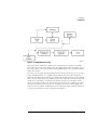
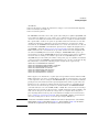
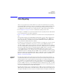
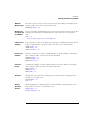
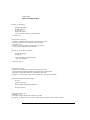
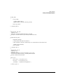
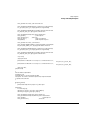
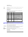
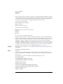
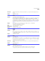
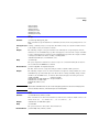
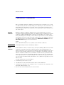
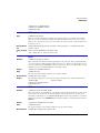
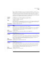
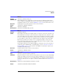
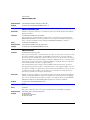
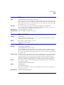
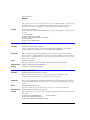
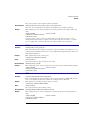
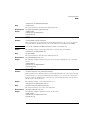
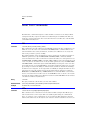
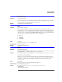
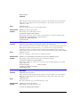
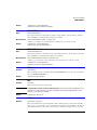
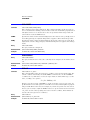
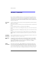
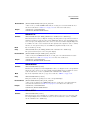
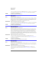
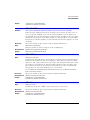
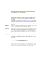
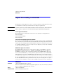
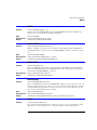
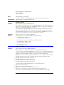
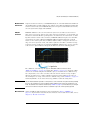
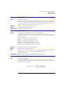
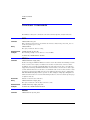
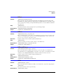
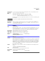
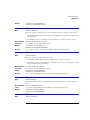
Data Flow
The data flow gives you an idea of where the measurements are made on the acquired data
and when the post-signal processing is applied to the data. The following figure is a block diagram of the instrument. The diagram is laid out serially for a visual perception of how the
data is affected by the instrument.
1-2
Introduction
Introduction
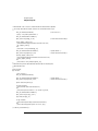
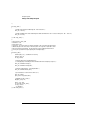
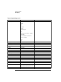
Figure 1-1. Sample Data Processing
The sample data is stored in the channel memory for further processing before being displayed. The time it takes for the sample data to be displayed depends on the number of post
processes you have selected. Averaging your sampled data helps remove any unwanted noise
from your waveform.
You can store your sample data in the instrument’s waveform memories for use as one of the
sources in Math functions, or to visually compare against a waveform that is captured at a
future time. The Math functions allow you to apply mathematical operations on your sampled
data. You can use these functions to duplicate many of the mathematical operations that your
circuit may be performing to verify that your circuit is operating correctly. The measurements section performs any of the automated measurements that are available in the instrument. The measurements that you have selected appear at the bottom of the display. The
Connect Dots section draws a straight line between sample data points, giving an analog look
to the waveform. This is sometimes called linear interpolation.
1-3
Introduction
Starting a Program
Starting a Program
The commands and syntax for initializing the instrument are listed in Chapter 3, “Common
Commands”. Refer to your GPIB manual and programming language reference manual for
information on initializing the interface. To make sure the bus and all appropriate interfaces
are in a known state, begin every program with an initialization statement. For example,
BASIC provides a CLEAR command which clears the interface buffer. When you are using
GPIB, CLEAR also resets the instrument's parser. After clearing the interface, initialize the
instrument to a preset state using the *RST command.
The AUTOSCALE command is very useful on unknown waveforms. It automatically sets up
the vertical channel, time base, and trigger level of the instrument.
A typical instrument setup configures the vertical range and offset voltage, the horizontal
range, delay time, delay reference, trigger mode, trigger level, and slope. An example of the
commands sent to the instrument are:
:CHANNEL1:RANGE 16;OFFSET 1.00<terminator>
:SYSTEM:HEADER OFF<terminator>
:TIMEBASE:RANGE 1E-3;DELAY 100E-6<terminator>
This example sets the time base at 1 ms full-scale (100 μs/div), with delay of 100 μs. Vertical
is set to 16 V full-scale (2 V/div), with center of screen at 1 V, and probe attenuation of 10.
The following program demonstrates the basic command structure used to program the
instrument.
10
20
30
40
50
60
70
80
90
100
110
120
CLEAR 707 ! Initialize instrument interface
OUTPUT 707;"*RST" !Initialize instrument to preset state
OUTPUT 707;":TIMEBASE:RANGE 5E-4"! Time base to 500 us full scale
OUTPUT 707;":TIMEBASE:DELAY 25E-9"! Delay to 25 ns
OUTPUT 707;":TIMEBASE:REFERENCE CENTER"! Display reference at center
OUTPUT 707;":CHANNEL1:RANGE .16"! Vertical range to 160 mV full scale
OUTPUT 707;":CHANNEL1:OFFSET -.04"! Offset to -40 mV
OUTPUT 707;":TRIGGER:LEVEL,-.4"! Trigger level to -0.4
OUTPUT 707;":TRIGGER:SLOPE POSITIVE"! Trigger on positive slope
OUTPUT 707;":SYSTEM:HEADER OFF"<terminator>
OUTPUT 707;":DISPLAY:GRATICULE FRAME"! Grid off
END
• Line 10 initializes the instrument interface to a known state and Line 20 initializes the
instrument to a preset state.
• Lines 30 through 50 set the time base, the horizontal time at 500 μs full scale, and 25 ns of
delay referenced at the center of the graticule.
• Lines 60 through 70 set the vertical range to 160 millivolts full scale and the center screen at
1-4
Introduction
Starting a Program
−40 millivolts.
• Lines 80 through 90 configure the instrument to trigger at −0.4 volts with normal triggering.
• Line 100 turns system headers off.
• Line 110 turns the grid off.
The DIGITIZE command is a macro that captures data using the acquisition (ACQUIRE) subsystem. When the digitize process is complete, the acquisition is stopped. The captured data
can then be measured by the instrument or transferred to the computer for further analysis.
The captured data consists of two parts: the preamble and the waveform data record. After
changing the instrument configuration, the waveform buffers are cleared. Before doing a
measurement, the DIGITIZE command should be sent to ensure new data has been collected.
You can send the DIGITIZE command with no parameters for a higher throughput. Refer to
the DIGITIZE command in Chapter 4, “Root Level Commands” for details. When the DIGITIZE command is sent to an instrument, the specified channel’s waveform is digitized with
the current ACQUIRE parameters. Before sending the :WAVEFORM:DATA? query to get
waveform data, specify the WAVEFORM parameters. The number of data points comprising a
waveform varies according to the number requested in the ACQUIRE subsystem. The
ACQUIRE subsystem determines the number of data points, type of acquisition, and number
of averages used by the DIGITIZE command. This allows you to specify exactly what the digitized information contains. The following program example shows a typical setup:
OUTPUT 707;":SYSTEM:HEADER OFF"<terminator>
OUTPUT 707;":WAVEFORM:SOURCE CHANNEL1"<terminator>
OUTPUT 707;":WAVEFORM:FORMAT BYTE"<terminator>
OUTPUT 707;":ACQUIRE:COUNT 8"<terminator>
OUTPUT 707;":ACQUIRE:POINTS 500"<terminator>
OUTPUT 707;":DIGITIZE CHANNEL1"<terminator>
OUTPUT 707;":WAVEFORM:DATA?"<terminator>
This setup places the instrument to acquire eight averages. This means that when the DIGITIZE command is received, the command will execute until the waveform has been averaged
at least eight times. After receiving the :WAVEFORM:DATA? query, the instrument will start
passing the waveform information when queried. Digitized waveforms are passed from the
instrument to the computer by sending a numerical representation of each digitized point.
The format of the numerical representation is controlled with the :WAVEFORM:FORMAT
command and may be selected as BYTE, WORD, or ASCII. The easiest method of entering a
digitized waveform depends on data structures, available formatting, and I/O capabilities. You
must scale the integers to determine the voltage value of each point. These integers are
passed starting with the leftmost point on the instrument's display. For more information,
refer to Chapter 25, “Waveform Commands”. When using GPIB, a digitize operation may be
aborted by sending a Device Clear over the bus (for example, CLEAR 707).
NOTE
The execution of the DIGITIZE command is subordinate to the status of ongoing limit tests. (See commands
ACQuire:RUNTil on page 6-4, MTEST:RUNTil on page 17-7, and LTEST:RUNTil on page 15-4.) The DIGITIZE
command will not capture data if the stop condition for a limit test has been met.
1-5
Introduction
Multiple Databases
Multiple Databases
Eye/Mask measurements are based on statistical data that is acquired and stored in the color
grade/gray scale database. The color grade/gray scale database consists of all data samples
displayed on the display graticule. The measurement algorithms are dependent upon histograms derived from the database. This database is internal to the instrument’s applications.
The color grade/gray scale database cannot be imported into an external database application.
If you want to perform an eye measurement, it is necessary that you first produce an eye diagram by triggering the instrument with a synchronous clock signal. Measurements made on a
pulse waveform while in Eye/Mask mode will fail.
Firmware revision A.03.00 and later allows for multiple color grade/gray scale databases to be
acquired and displayed simultaneously, including
• all four instrument channels
• all four math functions
• one saved color grade/gray scale file
The ability to use multiple databases allows for the comparison of
• channels to each other
• channels to a saved color grade/gray scale file
• functions to the channel data on which it is based
The advantage of acquiring and displaying channels and functions simultaneously is test
times are greatly reduced. For example, the time taken to acquire two channels in parallel is
approximately the same time taken to acquire a single channel.
Using Multiple
Most commands that control histograms, mask tests, or color grade data have additional
Databases in
optional parameters that were not available in firmware revisions prior to A.03.00. You can
Remote Programs use the commands to control a single channel or add the argument APPend to enable more
than one channel. The following example illustrates two uses of the CHANnel<n>:DISPlay
command.
SYSTem:MODE EYE
CHANnel1:DISPlay ON
CHANnel2:DISPlay ON
The result using the above set of commands, is Channel 1 cleared and disabled while Channel
2 is enabled and displayed. However, by adding the argument APPend to the last command of
the set, both Channels 1 and 2 will be enabled and displayed .
SYSTem:MODE EYE
CHANnel1:DISPlay ON
1-6
Introduction
Multiple Databases
CHANnel2:DISPlay ON,APPend
For a example of using multiple databases, refer to “multidatabase.c Sample Program” on
page 2-35.
Downloading a
Database
The general process for downloading a color grade/gray scale database is as follows:
1 Send the command :WAVEFORM:SOURCE CGRADE
This will select the color grade/gray scale database as the waveform source.
2 Issue :WAVeform:FORMat WORD.
Database downloads only support word formatted data (16-bit integers).
3 Send the query :WAVeform:DATA?
The data will be sent by means of a block data transfer as a two-dimensional array, 451 words
wide by 321 words high (refer to “Definite-Length Block Response Data” on page 1-26). The
data is transferred starting with the upper left pixel of the display graticule, column by column,
until the lower right pixel is transferred.
4 Send the command :WAVeform:XORigin to obtain the time of the left column.
5 Send the command :WAVeform:XINC to obtain the time increment of each column.
6 Send the command :WAVeform:YORigin to obtain the voltage or power of the vertical center
of the database.
7 Send the command :WAVeform:YORigin to obtain the voltage or power of the incremental row.
The information from steps 4 through 7 can also be obtained with the command :WAVeform:PREamble.
Auto Skew
Another multiple database feature is the auto skew. You can use the auto skew feature to set
the horizontal skew of multiple, active channels with the same bit rate, so that the waveform
crossings align with each other. This can be very convient when viewing multiple eye diagrams simultaneously. Slight differences between channels and test devices may cause a
phase difference between channels. Auto skew ensures that each eye is properly aligned, so
that measurements and mask tests can be properly executed.
In addition, auto skew optimizes the instrument trigger level. Prior to auto skew, at least one
channel must display a complete eye diagram in order to make the initial bit rate measurement. Auto skew requires more data to be sampled; therefore, acquisition time during auto
skew is slightly longer than acquisition time during measurements.
1-7
Introduction
Files
Files
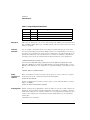
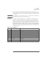
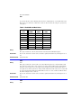
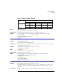
When specifying a file name in a remote command, enclose the name in double quotation
marks, such as "filename". If you specify a path, the path should be included in the quotation
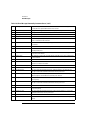
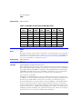
marks. All files stored using remote commands have file name extensions as listed in
Table 1-1. You can use the full path name, a relative path name, or no path.
If you do not specify an extension when storing a file, or specify an incorrect extension, it will
be corrected automatically according to the following rules:
• No extension specified: add the extension for the file type.
• Extension does not match file type: retain the filename, (including the current extension) and
add the appropriate extension.
You do not need to use an extension when loading a file if you use the optional destination
parameter. For example, :DISK:LOAD "STM1_OC3",SMASK will automatically add .msk to
the file name. ASCII waveform files can be loaded only if the file name explicitly includes the
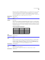
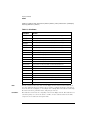
.txt extension. Table 1-2 on page 1-9 shows the rules used when loading a specified file.
If you don’t specify a directory when storing a file, the location of the file will be based on the
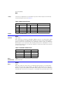
file type. Table 1-3 on page 1-10 shows the default locations for storing files. On 86100C
instruments, files are stored on the D: drive. On 86100A/B instruments, files are stored on the
C: drive.
When loading a file, you can specify the full path name, a relative path name, or no path
name. Table 1-4 on page 1-10 lists the rules for locating files, based on the path specified.
Standard masks loaded from D:\Scope\masks. Files may be stored to or loaded from any path
external drive or on any mapped network drive.
1-8
Introduction
Files
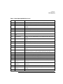
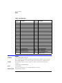
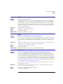
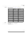
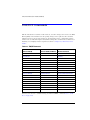
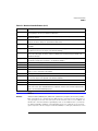
Table 1-1. File Name Extensions
File Type
File Name Extension
Waveform - internal format
.wfm
“STORe” on page 10-9
Waveform - text format (Verbose, XY Verbose,
or Y values)
.txt
“STORe” on page 10-9
Pattern Waveform
.csv
“PWAVeform:SAVE” on page 10-6
Setup
.set
“STORe” on page 10-9
Color grade - Gray Scale
.cgs
“STORe” on page 10-9
Jitter Memory
.jd
“STORe” on page 10-9
.bmp, .eps, .gif, .pcx, .ps, .jpg, .tif
“SIMage” on page 10-7
Mask
.msk, .pcm
“SAVE” on page 17-7
TDR/TDT
.tdr
“STORe” on page 10-9
MATLAB script
.m
“MATLab:SCRipt” on page 20-5
S-Parameter (Touchstone format)
.s1p, .s2p
“SPARameter:SAVE” on page 10-8
S-Parameter (text format)
.txt
“SPARameter:SAVE” on page 10-8
Screen image
a
Command
a. For .gif and .tif file formats, this instrument uses LZW compression/decompression licensed under U.S. patent No
4,558,302 and foreign counterparts. End user should not modify, copy, or distribute LZW compression/decompression capability. For .jpg file format, this instrument uses the .jpg software written by the Independent JPEG Group.
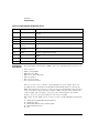
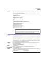
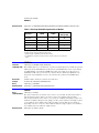
Table 1-2. Rules for Loading Files
File Name Extension
Destination
Rule
No extension
Not specified
Default to internal waveform format; add .wfm extension
Extension does not match file type
Not specified
Default to internal waveform format; add .wfm extension
Extension matches file type
Not specified
Use file name with no alterations; destination is based on extension
file type
No extension
Specified
Add extension for destination type; default for waveforms is internal
format (.wfm)
Extension does not match destination
file type
Specified
Retain file name; add extension for destination type. Default for
waveforms is internal format (.wfm)
Extension matches destination file
type
Specified
Retain file name; destination is as specified
1-9
Introduction
Files
Table 1-3. Default File Locations
File Type
Default Location
Waveform - internal format, text format (Verbose, XY Verbose, or Y
values),
D:\User Files\waveforms
Pattern Waveforms
D:\User Files\waveforms
Setup
D:\User Files\setups
Color Grade - Gray Scale
D:\User Files\colorgrade-grayscale
Jitter Memory
D:\User Files\jitter data
Screen Image
D:\User Files\screen images
Mask
C:\Scope\masks (standard masks)
D:\User Files\masks (user-defined masks)
TDR/TDT calibration data (software revision A.05.00 and below)
D:\User Files\TDR normalization
TDR/TDT calibration data (software revision A.06.00 and above)
D:\User Files\TDR calibration
MATLAB script
D:\User Files\Matlab scripts
S-Parameters
D:\User Files\S-parameter data
Table 1-4. File Locations (Loading Files)
File Name
Rule
Full path name
Use file name and path specified
Relative path name
Full path name is formed relative to the present working directory, set with the command :DISK:CDIR. The
present working directory can be read with the query :DISK:PWD?
File name with no
preceding path
Add the file name to the default path (D:\User Files) based on the file type. (C drive on 86100A/B
instruments.)
1-10
Introduction
Status Reporting
Status Reporting
Almost every program that you write will need to monitor the instrument for its operating
status. This includes querying execution or command errors and determining whether or not
measurements have been completed. Several status registers and queues are provided to
accomplish these tasks. In this section, you’ll learn how to enable and read these registers.
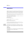
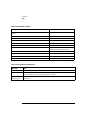
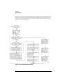
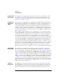
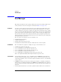
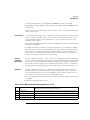
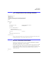
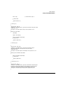
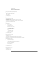
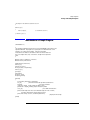
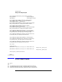
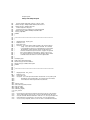
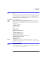
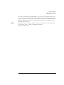
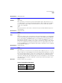
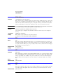
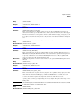
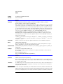
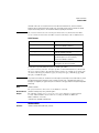
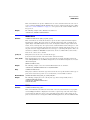
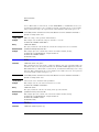
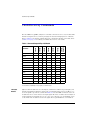
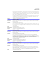
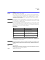
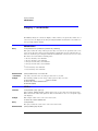
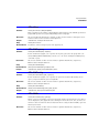
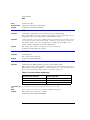
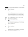
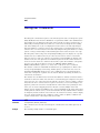
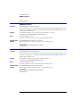
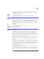
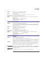
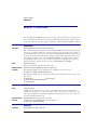
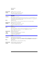
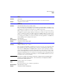
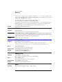
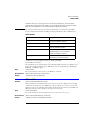
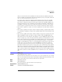
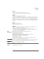
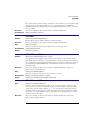
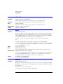
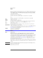
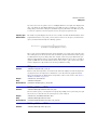
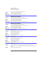
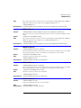
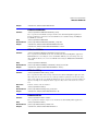
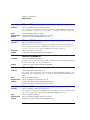
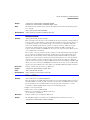
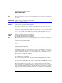
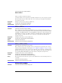
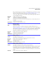
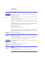
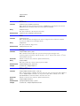
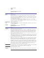
• Refer to Figure 1-4 on page 1-14 for an overall status reporting decision chart.
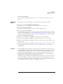
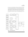
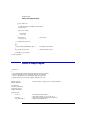
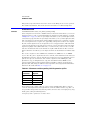
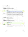
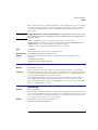
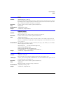
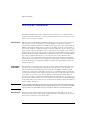
• See Figure 1-3 and Figure 1-4 to learn the instrument's status reporting structure which allows
you to monitor specific events in the instrument.
• Table 1-5 on page 1-17 lists the bit definitions for each bit in the status reporting data structure.
The Status Byte Register, the Standard Event Status Register group, and the Output Queue
are defined as the Standard Status Data Structure Model in IEEE 488.2-1987. IEEE 488.2
defines data structures, commands, and common bit definitions for status reporting. There
are also instrument-defined structures and bits.
To monitor an event, first clear the event, then enable the event. All of the events are cleared
when you initialize the instrument. To generate a service request (SRQ) interrupt to an
external computer, enable at least one bit in the Status Byte Register. To make it possible for
any of the Standard Event Status Register bits to generate a summary bit, the corresponding
bits must be enabled. These bits are enabled by using the *ESE common command to set the
corresponding bit in the Standard Event Status Enable Register. To generate a service
request (SRQ) interrupt to the computer, at least one bit in the Status Byte Register must be
enabled. These bits are enabled by using the *SRE common command to set the corresponding bit in the Service Request Enable Register. These enabled bits can then set RQS and MSS
(bit 6) in the Status Byte Register. For more information about common commands, see
Chapter 3, “Common Commands”.
Status Byte
Register
The Status Byte Register is the summary-level register in the status reporting structure. It
contains summary bits that monitor activity in the other status registers and queues. The Status Byte Register is a live register. That is, its summary bits are set and cleared by the presence and absence of a summary bit from other event registers or queues. If the Status Byte
Register is to be used with the Service Request Enable Register to set bit 6 (RQS/MSS) and to
generate an SRQ, at least one of the summary bits must be enabled, then set. Also, event bits
in all other status registers must be specifically enabled to generate the summary bit that sets
the associated summary bit in the Status Byte Register.
The Status Byte Register can be read using either the *STB? common command query or the
GPIB serial poll command. Both commands return the decimal-weighted sum of all set bits in
the register. The difference between the two methods is that the serial poll command reads
1-11
Introduction
Status Reporting
bit 6 as the Request Service (RQS) bit and clears the bit which clears the SRQ interrupt. The
*STB? query reads bit 6 as the Master Summary Status (MSS) and does not clear the bit or
have any affect on the SRQ interrupt. The value returned is the total bit weights of all of the
bits that are set at the present time.
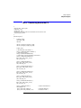
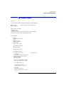
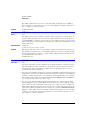
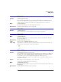
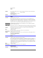
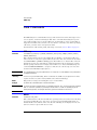
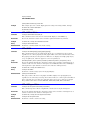
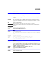
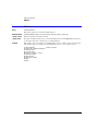
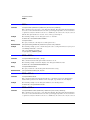
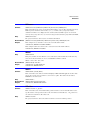
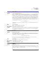
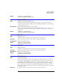
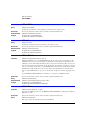
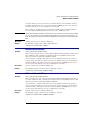
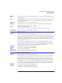
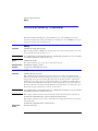
Figure 1-2. Status Reporting Decision Chart
1-12
Introduction
Status Reporting
The use of bit 6 can be confusing. This bit was defined to cover all possible computer interfaces, including a computer that could not do a serial poll. The important point to remember
is that, if you are using an SRQ interrupt to an external computer, the serial poll command
clears bit 6. Clearing bit 6 allows the instrument to generate another SRQ interrupt when
another enabled event occurs. The only other bit in the Status Byte Register affected by the
*STB? query is the Message Available bit (bit 4). If there are no other messages in the Output
Queue, bit 4 (MAV) can be cleared as a result of reading the response to the *STB? query.
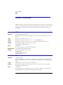
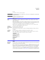
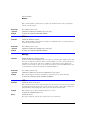
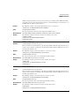
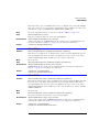
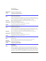
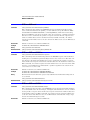
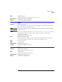
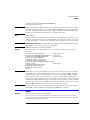
If bit 4 (weight = 16) and bit 5 (weight = 32) are set, a program would print the sum of the
two weights. Since these bits were not enabled to generate an SRQ, bit 6 (weight = 64) is not
set.
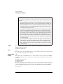
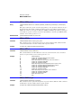
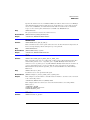
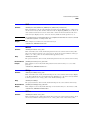
Figure 1-3. Status Reporting Overview
1-13
Introduction
Status Reporting
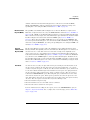
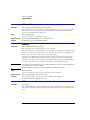
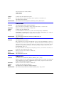
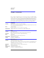
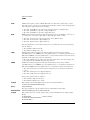
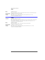
Figure 1-4. Status Reporting Data Structures
1-14
Introduction
Status Reporting
Status Reporting Data Structures (continued)
1-15
Introduction
Status Reporting
This BASIC example uses the *STB? query to read the contents of the instrument’s Status
Byte Register when none of the register's summary bits are enabled to generate an SRQ interrupt.
10
20
30
40
OUTPUT 707;":SYSTEM:HEADER OFF;*STB?"!Turn headers off
ENTER 707;Result!Place result in a numeric variable
PRINT Result!Print the result
End
The next program prints 132 and clears bit 6 (RQS) of the Status Byte Register. The difference in the decimal value between this example and the previous one is the value of bit 6
(weight = 64). Bit 6 is set when the first enabled summary bit is set, and is cleared when the
Status Byte Register is read by the serial poll command.
This example uses the BASIC serial poll (SPOLL) command to read the contents of the
instrument’s Status Byte Register.
10
20
30
Result = SPOLL(707)
PRINT Result
END
Use Serial Polling to Read the Status Byte Register. Serial polling is the preferred method to
read the contents of the Status Byte Register because it resets bit 6 and allows the next
enabled event that occurs to generate a new SRQ interrupt.
Service Request
Enable Register
Setting the Service Request Enable Register bits enables corresponding bits in the Status
Byte Register. These enabled bits can then set RQS and MSS (bit 6) in the Status Byte Register. Bits are set in the Service Request Enable Register using the *SRE command, and the
bits that are set are read with the *SRE? query. Bit 6 always returns 0. Refer to the Status
Reporting Data Structures shown in Figure 1-4This example sets bit 4 (MAV) and bit 5 (ESB)
in the Service Request Enable Register.
OUTPUT 707;"*SRE 48"
This example uses the parameter “48” to allow the instrument to generate an SRQ interrupt
under the following conditions:
• When one or more bytes in the Output Queue set bit 4 (MAV).
• When an enabled event in the Standard Event Status Register generates a summary bit that
sets bit 5 (ESB).
Trigger Event
Register (TRG)
This register sets the TRG bit in the status byte when a trigger event occurs. The TRG event
register stays set until it is cleared by reading the register or using the *CLS (clear status)
command. If your application needs to detect multiple triggers, the TRG event register must
be cleared after each one. If you are using the Service Request to interrupt a computer operation when the trigger bit is set, you must clear the event register after each time it is set.
1-16
Introduction
Status Reporting
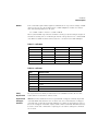
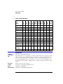
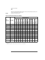
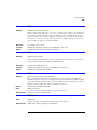
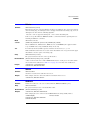
Table 1-5. Status Reporting Bit Definition (1 of 2)
Bit
Description
Definition
ACQ
Acquisition
Indicates that acquisition test has completed in the Acquisition Register.
AREQD
Autoscale Required
Indicates that a parameter change in Jitter Mode has made an autoscale necessary.
CLCK
CloCk
Indicates that one of the enabled conditions in the Clock Recovery Register has
occurred.
CME
Command Error
Indicates if the parser detected an error.
COMP
Complete
Indicates the specified test has completed.
DDE
Device Dependent Error
Indicates if the device was unable to complete an operation for device dependent
reasons.
EFAIL
Edge Characterization
Fail
Indicates that the characterizing of edges in Jitter Mode has failed.
ESB
Event Status Bit
Indicates if any of the enabled conditions in the Standard Event Status Register have
occurred.
EXE
Execution Error
Indicates if a parameter was out of range or was inconsistent with the current
settings.
FAIL
Fail
Indicates the specified test has failed.
JLOSS
Pattern Synchronization
Loss
Indicates that the pattern synchronization is lost in Jitter Mode.
LCL
Local
Indicates if a remote-to-local transition occurs.
LOCK
LOCKed
Indicates that a locked or trigger capture condition has occurred in the Clock Recovery
Module.
LOSS
Time Reference Loss
Indicates the Precision Timebase (provided by the Agilent 86107A module) has
detected a time reference loss due to a change in the reference clock signal.
LTEST
Limit Test
Indicates that one of the enabled conditions in the Limit Test Register has occurred.
MAV
Message Available
Indicates if there is a response in the output queue.
MSG
Message
Indicates if an advisory has been displayed.
MSS
Master Summary Status
Indicates if a device has a reason for requesting service.
MTEST
Mask Test
Indicates that one of the enabled conditions in the Mask Test Register has occurred.
NSPR1
No Signal Present
Receiver 1
Indicates that the Clock Recovery Module has detected the loss of an optical signal on
receiver one.
NSPR2
No Signal Present
Receiver 2
Indicates that the Clock Recovery Module has detected the loss of an optical signal on
receiver two.
OPC
Operation Complete
Indicates if the device has completed all pending operations.
OPER
Operation Status
Register
Indicates if any of the enabled conditions in the Operation Status Register have
occurred.
PON
Power On
Indicates power is turned on.
1-17
Introduction
Status Reporting
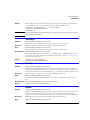
Table 1-5. Status Reporting Bit Definition (2 of 2)
Bit
Description
Definition
PTIME
Precision Timebase
Indicates that one of the enabled conditions in the Precision Timebase Register has
occurred.
QYE
Query Error
Indicates if the protocol for queries has been violated.
RQL
Request Control
Indicates if the device is requesting control.
RQS
Request Service
Indicates that the device is requesting service.
SPR1
Signal Present
Receiver 1
Indicates that the Clock Recovery Module has detected an optical signal on receiver
one.
SPR2
Signal Present
Receiver 2
Indicates that the Clock Recovery Module has detected an optical signal on receiver
two.
TRG
Trigger
Indicates if a trigger has been received.
UNLK
UNLoCKed
Indicates that an unlocked or trigger loss condition has occurred in the Clock Recovery
Module.
URQ
USR
Not used. Permanently set to zero.
User Event Register
Standard Event
Status Register
Indicates if any of the enabled conditions have occurred in the User Event Register.
The Standard Event Status Register (SESR) monitors the following instrument status events:
•
•
•
•
•
•
•
PON - Power On
CME - Command Error
EXE - Execution Error
DDE - Device Dependent Error
QYE - Query Error
RQC - Request Control
OPC - Operation Complete
When one of these events occurs, the corresponding bit is set in the register. If the corresponding bit is also enabled in the Standard Event Status Enable Register, a summary bit
(ESB) in the Status Byte Register is set. The contents of the Standard Event Status Register
can be read and the register cleared by sending the *ESR? query. The value returned is the
total bit weights of all of the bits set at the present time. If bit 4 (weight = 16) and bit 5
(weight = 32) are set, the program prints the sum of the two weights.
This example uses the *ESR? query to read the contents of the Standard Event Status Register.
10
20
30
40
50
1-18
OUTPUT 707;":SYSTEM:HEADER OFF"!Turn headers off
OUTPUT 707;"*ESR?"
ENTER 707;Result!Place result in a numeric variable
PRINT Result!Print the result
End
Introduction
Status Reporting
Standard Event
Status Enable
Register
For any of the Standard Event Status Register (SESR) bits to generate a summary bit, you
must first enable the bit. Use the *ESE (Event Status Enable) common command to set the
corresponding bit in the Standard Event Status Enable Register. Set bits are read with the
*ESE? query. Suppose your application requires an interrupt whenever any type of error
occurs. The error status bits in the Standard Event Status Register are bits 2 through 5. The
sum of the decimal weights of these bits is 60. Therefore, you can enable any of these bits to
generate the summary bit by sending:
OUTPUT 707;"*ESE 60"
Whenever an error occurs, the instrument sets one of these bits in the Standard Event Status
Register. Because the bits are all enabled, a summary bit is generated to set bit 5 (ESB) in the
Status Byte Register. If bit 5 (ESB) in the Status Byte Register is enabled (via the *SRE command), a service request interrupt (SRQ) is sent to the external computer.
NOTE
Disabled SESR Bits Respond, but Do Not Generate a Summary Bit. Standard Event Status Register bits that are
not enabled still respond to their corresponding conditions (that is, they are set if the corresponding event
occurs). However, because they are not enabled, they do not generate a summary bit in the Status Byte Register.
User Event
Register (UER)
This register hosts the LCL bit (bit 0) from the Local Events Register. The other 15 bits are
reserved. You can read and clear this register using the UER? query. This register is enabled
with the UEE command. For example, if you want to enable the LCL bit, you send a mask
value of 1 with the UEE command; otherwise, send a mask value of 0.
Local Event
Register (LCL)
This register sets the LCL bit in the User Event Register and the USR bit (bit 1) in the Status
byte. It indicates a remote-to-local transition has occurred. The LER? query is used to read
and to clear this register.
Operation Status
Register (OPR)
This register hosts the CLCK bit (bit 7), the LTEST bit (bit 8), the ACQ bit (bit 9) and the
MTEST bit (bit 10). The CLCK bit is set when any of the enabled conditions in the Clock
Recovery Event Register have occurred. The LTEST bit is set when a limit test fails or is completed and sets the corresponding FAIL or COMP bit in the Limit Test Events Register. The
ACQ bit is set when the COMP bit is set in the Acquisition Event Register, indicating that the
data acquisition has satisfied the specified completion criteria. The MTEST bit is set when
the Mask Test either fails specified conditions or satisfies its completion criteria, setting the
corresponding FAIl or COMP bits in the Mask Test Events Register. The PTIME bit is set
when there is a loss of the precision timebase reference occurs setting a bit in the Precision
Timebase Events Register. The JIT bit is set in Jitter Mode when a bit is set in the Jitter
Events Register. This occurs when there is a failure or an autoscale is needed. If any of these
bits are set, the OPER bit (bit 7) of the Status Byte register is set. The Operation Status Register is read and cleared with the OPER? query. The register output is enabled or disabled
using the mask value supplied with the OPEE command.
1-19
Introduction
Status Reporting
Acquisition Event Bit 0 (COMP) of the Acquisition Event Register is set when the acquisition limits complete.
Register (AER)
The Acquisition completion criteria are set by the ACQuire:RUNtil command. Refer to
“RUNTil” on page 6-4. The Acquisition Event Register is read and cleared with the ALER?
query. Refer to “ALER?” on page 4-3.
Clock Recovery
Event Register
(CRER)
This register hosts the UNLK bit (bit 0), LOCK bit (bit 1), NSPR1 bit (bit 2), SPR1 bit (bit 3),
NSPR2 bit (bit 4) and SPR2 (bit 5). Bit 0 (UNLK) of the Clock Recovery Event Register is set
when an 83491/2/3/4/5/6A clock recovery module becomes unlocked or trigger loss has
occurred. Bit 1 (LOCK) of the Clock Recovery Event Register is set when a clock recovery
module becomes locked or a trigger capture has occurred. If an 83496A module is locked,
sending the CRECovery:RELock command does not set UNLK bit (bit 0) or LOCK bit (bit 1).
To determine if the RELock command has completed, use the CRECovery:LOCKed? query.
Refer to “RELock” on page 9-9.
Bits 2 through 5 provide information on optical signals and so are not effected by 83495A
modules. Bit 2 (NSPR1) of the Clock Recovery Event Register is set when an clock recovery
module transitions to no longer detecting an optical signal on receiver one. Bit 3 (SPR1) of
the Clock Recovery Event Register is set when an clock recovery module transitions to
detecting an optical signal on receiver one. Bit 4 (NSPR2) of the Clock Recovery Event Register is set when an clock recovery module transitions to no longer detecting an optical signal
on receiver two. Bit 5 (SPR2) of the Clock Recovery Event Register is set when an clock
recovery module transitions to detecting an optical signal on receiver two. The Clock Recovery Event Register is read and cleared with the CRER? query. Refer to “CRER?” on page 4-6.
When either of the UNLK, LOCK, NSPR1, SPR1, NSPR2 or SPR2 bits are set, they in turn set
CLCK bit (bit 7) of the Operation Status Register. Results from the Clock Recovery Event
Register can be masked by using the CREE command to set the Clock Recovery Event
Enable Register. Refer to Refer to “CREE” on page 4-5 for enable and mask value definitions.
Limit Test Event
Register (LTER)
Bit 0 (COMP) of the Limit Test Event Register is set when the Limit Test completes. The
Limit Test completion criteria are set by the LTESt:RUN command. Refer to “RUNTil” on
page 15-4. Bit 1 (FAIL) of the Limit Test Event Register is set when the Limit Test fails. Failure criteria for the Limit Test are defined by the LTESt:FAIL command. Refer to “FAIL” on
page 15-2. The Limit Test Event Register is read and cleared with the LTER? query. Refer to
“LTER?” on page 4-9. When either the COMP or FAIL bits are set, they in turn set the LTEST
bit (bit 8) of the Operation Status Register. You can mask the COMP and FAIL bits, thus preventing them from setting the LTEST bit, by defining a mask using the LTEE command. Refer
to “LTEE” on page 4-9. When the COMP bit is set, it in turn sets the ACQ bit (bit 9) of the
Operation Status Register. Results from the Acquisition Register can be masked by using the
AEEN command to set the Acquisition Event Enable Register to the value 0. You enable the
COMP bit by setting the mask value to 1.
Jitter Event
Register (JIT)
Bit 0 (EFAIL) of the Jitter Event Register is set when characterizing edges in Jitter Mode
fails. Bit 1 (JLOSS) of the register is set when pattern synchronization is lost in Jitter Mode.
Bit 2 (AREQD) of the register is set when a parameter change in Jitter Mode has made
autoscale necessary. Bit 12 of the Operation Status Register (JIT) indicates that one of the
1-20
Introduction
Status Reporting
enabled conditions in the Jitter Event Register has occurred. You can mask the EFAIL,
JLOSS, and AREQD bits, thus preventing them from setting the JIT bit, by setting corresponding bits to zero using the JEE command. Refer to “JEE” on page 4-7.
Mask Test Event
Register (MTER)
Bit 0 (COMP) of the Mask Test Event Register is set when the Mask Test completes. The
Mask Test completion criteria are set by the MTESt:RUNTil command. Refer to “RUNTil” on
page 17-6. Bit 1 (FAIL) of the Mask Test Event Register is set when the Mask Test fails. This
will occur whenever any sample is recorded within any region defined in the mask. The Mask
Test Event Register is read and cleared with the MTER? query. Refer to “MTER?” on
page 4-10. When either the COMP or FAIL bits are set, they in turn set the MTEST bit (bit
10) of the Operation Status Register. You can mask the COMP and FAIL bits, thus preventing
them from setting the MTEST bit, by setting corresponding bits to zero using the MTEE command. Refer to “MTEE” on page 4-10.
Precision
Timebase Event
Register (PTER)
The Precision Timebase feature requires the installation of the Agilent 86107A Precision
Timebase Module. Bit 0 (LOSS) of the Precision Timebase Event Register is set when loss of
the time reference occurs. Time reference is lost when a change in the amplitude or frequency of the reference clock signal is detected. The Precision Timebase Event Register is
read and cleared with the PTER? query. Refer to “PTER?” on page 4-12. When the LOSS bit is
set, it in turn sets the PTIME bit (bit 11) of the Operation Status Register. Results from the
Precision Timebase Register can be masked by using the PTEE command to set the Precision
Timebase Event Enable Register to the value 0. You enable the LOSS bit by setting the mask
value to 1. Refer to “PTEE” on page 4-11.
Error Queue
As errors are detected, they are placed in an error queue. This queue is first in, first out. If
the error queue overflows, the last error in the queue is replaced with error –350, “Queue
overflow”. Any time the queue overflows, the oldest errors remain in the queue, and the most
recent error is discarded. The length of the instrument's error queue is 30 (29 positions for
the error messages, and 1 position for the “Queue overflow” message). The error queue is
read with the SYSTEM:ERROR? query. Executing this query reads and removes the oldest
error from the head of the queue, which opens a position at the tail of the queue for a new
error. When all the errors have been read from the queue, subsequent error queries return 0,
“No error.” The error queue is cleared when any of the following occurs:
• When the instrument is powered up.
• When the instrument receives the *CLS common command.
• When the last item is read from the error queue.
For more information on reading the error queue, refer to the SYSTEM:ERROR? query in
Chapter 5, “System Commands”. For a complete list of error messages, refer to “Error Messages” on page 1-46.
1-21
Introduction
Status Reporting
Output Queue
The output queue stores the instrument-to-computer responses that are generated by certain instrument commands and queries. The output queue generates the Message Available
summary bit when the output queue contains one or more bytes. This summary bit sets the
MAV bit (bit 4) in the Status Byte Register. The output queue may be read with the BASIC
ENTER statement.
Message Queue
The message queue contains the text of the last message written to the advisory line on the
screen of the instrument. The queue is read with the SYSTEM:DSP? query. Note that messages sent with the SYSTem:DSP command do not set the MSG status bit in the Status Byte
Register.
Clearing
Registers and
Queues
The *CLS common command clears all event registers and all queues except the output
queue. If *CLS is sent immediately following a program message terminator, the output
queue is also cleared.
1-22
Introduction
Command Syntax
Command Syntax
In accordance with IEEE 488.2, the instrument’s commands are grouped into “subsystems.”
Commands in each subsystem perform similar tasks. Starting with Chapter 5, “System Commands” each chapter covers a separate subsystem.
Sending a
Command
It’s easy to send a command to the instrument. Simply create a command string from the
commands listed in this book, and place the string in your program language’s output statement. For commands other than common commands, include a colon before the subsystem
name. For example, the following string places the cursor on the peak laser line and returns
the power level of this peak:
OUTPUT 720;”:MEAS:SCAL:POW? MAX”
Commands can be sent using any combination of uppercase or lowercase ASCII characters.
Instrument responses, however, are always returned in uppercase.
The program instructions within a data message are executed after the program message terminator is received. The terminator may be either a NL (new line) character, an EOI (EndOr-Identify) asserted in the GPIB interface, or a combination of the two. Asserting the EOI
sets the EOI control line low on the last byte of the data message. The NL character is an
ASCII linefeed (decimal 10). The NL (New Line) terminator has the same function as an EOS
(End Of String) and EOT (End Of Text) terminator.
Short or Long
Forms
Commands and queries may be sent in either long form (complete spelling) or short form
(abbreviated spelling). The description of each command in this manual shows both versions;
the extra characters for the long form are shown in lowercase. However, commands can be
sent using any combination of uppercase or lowercase ASCII characters. Instrument
responses, however, are always returned in uppercase. Programs written in long form are
easily read and are almost self-documenting. Using short form commands conserves the
amount of controller memory needed for program storage and reduces the amount of I/O
activity.
The short form is the first four characters of the keyword, unless the fourth character is a
vowel. Then the mnemonic is the first three characters of the keyword. If the length of the
keyword is four characters or less, this rule does not apply, and the short form is the same as
the long form.
For example:
:TIMEBASE:DELAY 1E-6 is the long form.
:TIM:DEL 1E-6 is the short form.
1-23
Introduction
Command Syntax
.
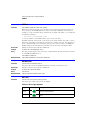
Table 1-6. Long and Short Command Forms
Long Form
Short Form
How the Rule is Applied
RANGE
RANG
Short form is the first four characters of the keyword.
PATTERN
PATT
Short form is the first four characters of the keyword.
DISK
DISK
Short form is the same as the long form.
DELAY
DEL
Fourth character is a vowel, short form is the first three characters.
White Space
White space is defined to be one or more characters from the ASCII set of 0 through 32 decimal, excluding 10 (NL). White space is usually optional, and can be used to increase the readability of a program.
Combining
Commands
You can combine commands from the same subsystem provided that they are both on the
same level in the subsystem’s hierarchy. Simply separate the commands with a semi-colon (;).
If you have selected a subsystem, and a common command is received by the instrument, the
instrument remains in the selected subsystem. For example, the following commands turn
averaging on, then clears the status information without leaving the selected subsystem.
":ACQUIRE:AVERAGE ON;*CLS;COUNT 1024"
You can send commands and program queries from different subsystems on the
same line. Simply precede the new subsystem by a semicolon followed by a colon.
Multiple commands may be any combination of compound and simple commands. For example:
:CHANNEL1:RANGE 0.4;:TIMEBASE:RANGE 1
Adding
parameters to a
command
Many commands have parameters that specify an option. Use a space character to separate
the parameter from the command as shown in the following line:
OUTPUT 720;”:INIT:CONT ON”
Separate multiple parameters with a comma (,). Spaces can be added around the commas to
improve readability.
OUTPUT 720;”:MEAS:SCAL:POW:FREQ? 1300, MAX”
String Arguments Strings contain groups of alphanumeric characters which are treated as a unit of data by the
instrument. You may delimit embedded strings with either single (') or double (") quotation
marks. These strings are case-sensitive, and spaces act as legal characters just like any other
character. For example, this command writes the line string argument to the instrument’s
advisory line:
:SYSTEM:DSP ""This is a message.""
1-24
Introduction
Command Syntax
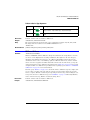
Numbers
Some commands require number arguments. All numbers are expected to be strings of ASCII
characters. You can use exponential notation or suffix multipliers to indicate the numeric
value. The following numbers are all equal:
28 = 0.28E2 = 280E-1 = 28000m = 0.028K = 28E-3K
When a syntax definition specifies that a number is an integer, any fractional part is ignored
and truncated. Using "mV" or "V" following the numeric voltage value in some commands will
cause Error 138–Suffix not allowed. Instead, use the convention for the suffix multiplier.
.
Table 1-7. <suffix mult>
Value
Mnemonic
Value
Mnemonic
1E18
EX
1E-3
m
1E15
PE
1E-6
u
1E12
T
1E-9
n
1E9
G
1E-12
p
1E6
MA
1E-15
f
1E3
K
1E-18
a
Table 1-8. <suffix unit>
Suffix
Referenced Unit
V
Volt
s
Second
W
Watt
BIT
Bits
dB
Decibel
%
Percent
Hz
Hertz
Infinity
Representation
The representation for infinity for this instrument is 9.99999E+37. This is also the value
returned when a measurement cannot be made.
Sequential and
Overlapped
Commands
IEEE 488.2 makes a distinction between sequential and overlapped commands. Sequential
commands finish their task before the execution of the next command starts. Overlapped
commands run concurrently. Commands following an overlapped command may be started
before the overlapped command is completed. The common commands *WAI and *OPC may
be used to ensure that commands are completely processed before subsequent commands
are executed.
1-25
Introduction
Command Syntax
Definite-Length
Block Response
Data
Definite-length block response data allows any type of device-dependent data to be transmitted over the system interface as a series of 8-bit binary data bytes. This is particularly useful
for sending large quantities of data or 8-bit extended ASCII codes. The syntax is a pound sign
(#) followed by a non-zero digit representing the number of digits in the decimal integer.
After the non-zero digit is the decimal integer that states the number of 8-bit data bytes being
sent. This is followed by the actual data. For example, for transmitting 4000 bytes of data, the
syntax would be:
#44000 <4000 bytes of data> <terminator>
The leftmost “4” represents the number of digits in the number of bytes, and “4000” represents the number of bytes to be transmitted.
Queries
Command headers immediately followed by a question mark (?) are queries. After receiving a
query, the instrument interrogates the requested subsystem and places the answer in its output queue. The answer remains in the output queue until it is read or until another command
is issued. When read, the answer is transmitted across the bus to the designated listener
(typically a computer). For example, the query:
:TIMEBASE:RANGE?
places the current time base setting in the output queue. In BASIC, the computer input statement:
ENTER < device address >;Range
passes the value across the bus to the computer and places it in the variable Range. You can
use query commands to find out how the instrument is currently configured. They are also
used to get results of measurements made by the instrument. For example, the command:
:MEASURE:RISETIME?
tells the instrument to measure the rise time of your waveform and place the result in the
output queue. The output queue must be read before the next program message is sent. For
example, when you send the query :MEASURE:RISETIME? you must follow it with an input
statement. In BASIC, this is usually done with an ENTER statement immediately followed by
a variable name. This statement reads the result of the query and places the result in a specified variable. If you send another command or query before reading the result of a query, the
output buffer is cleared and the current response is lost. This also generates a query-interrupted error in the error queue. If you execute an input statement before you send a query, it
will cause the computer to wait indefinitely.
If a measurement cannot be made because of the lack of data, because the source signal is
not displayed, the requested measurement is not possible (for example, a period measurement on an FFT waveform), or for some other reason, 9.99999E+37 is returned as the measurement result. In TDR mode with ohms specified, the returned value is 838MΩ.
You can send multiple queries to the instrument within a single program message, but you
must also read them back within a single program message. This can be accomplished by
either reading them back into a string variable or into multiple numeric variables. For example, you could read the result of the query :TIMEBASE:RANGE?;DELAY? into the string variable Results$ with the command: ENTER 707;Results$
1-26
Introduction
Command Syntax
When you read the result of multiple queries into string variables, each response is separated
by a semicolon. For example, the response of the query :TIMEBASE:RANGE?;DELAY? would
be:
<range_value>;<delay_value>
Use the following program message to read the query :TIMEBASE:RANGE?;DELAY? into
multiple numeric variables:
ENTER 707;Result1,Result2
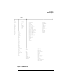
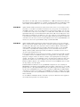
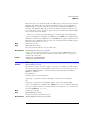
The Command
Tree
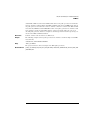
The command tree in Figure 1-5 on page 1-29 shows all of the commands in the
Agilent 86100A and the relationship of the commands to each other. The IEEE 488.2 common commands do not affect the position of the parser within the tree.
A leading colon or a program message terminator (<NL> or EOI true on the last byte) places
the parser at the root of the command tree. A leading colon is a colon that is the first character of a program header. Executing a subsystem command places you in that subsystem until
a leading colon or a program message terminator is found.
The commands in this instrument can be placed into three types: common commands, root
level commands, and subsystem commands.
• Common commands (defined by IEEE 488.2) control functions that are common to all IEEE
488.2 instruments. These commands are independent of the tree and do not affect the position
of the parser within the tree. *RST is an example of a common command.
• Root level commands control many of the basic functions of the instrument. These commands
reside at the root of the command tree. They can always be parsed if they occur at the beginning of a program message or are preceded by a colon. Unlike common commands, root level
commands place the parser back at the root of the command tree. AUTOSCALE is an example
of a root level command.
• Subsystem commands are grouped together under a common node of the command tree, such
as the TIMEBASE commands. Only one subsystem may be selected at a given time. When the
instrument is initially turned on, the command parser is set to the root of the command tree
and no subsystem is selected.
Command headers are created by traversing down the command tree. A legal command
header from the command tree would be :TIMEBASE:RANGE. It consists of the subsystem
followed by a command separated by colons. The compound header contains no spaces.
In the command tree, use the last mnemonic in the compound header as a reference point
(for example, RANGE). Then find the last colon above that mnemonic (TIMEBASE:). That is
the point where the parser resides. Any command below this point can be sent within the
current program message without sending the mnemonics which appear above them (for
example, REFERENCE).
Use a colon to separate two commands in the same subsystem.
OUTPUT 707;":CHANNEL1:RANGE 0.5;OFFSET 0"
1-27
Introduction
Command Syntax
The colon between CHANNEL1 and RANGE is necessary because CHANNEL1:RANGE specifies a command in a subsystem. The semicolon between the RANGE command and the OFFSET command is required to separate the two commands. The OFFSET command does not
need CHANNEL1 preceding it because the CHANNEL1:RANGE command sets the parser to
the CHANNEL1 node in the tree.
1-28
Introduction
Command Syntax
Figure 1-5. Command Tree
1-29
Introduction
Command Syntax
Command Tree (Continued)
1-30
Introduction
Command Syntax
Command Tree (Continued)
1-31
Introduction
Command Syntax
Command Tree (Continued)
1-32
Introduction
Command Syntax
Command Tree (Continued)
1-33
Introduction
Interface Functions
Interface Functions
The interface functions deal with general bus management issues, as well as messages that
can be sent over the bus as bus commands. In general, these functions are defined by IEEE
488.1. The instrument is equipped with a GPIB interface connector on the rear panel. This
allows direct connection to a GPIB equipped computer. You can connect an external GPIB
compatible device to the instrument by installing a GPIB cable between the two units. Finger
tighten the captive screws on both ends of the GPIB cable to avoid accidentally disconnecting
the cable during operation. A maximum of fifteen GPIB compatible instruments (including a
computer) can be interconnected in a system by stacking connectors. This allows the instruments to be connected in virtually any configuration, as long as there is a path from the computer to every device operating on the bus. The interface capabilities of this instrument, as
defined by IEEE 488.1, are listed in the Table 1-9 on page 1-35.
CAUTION
Avoid stacking more than three or four cables on any one connector. Multiple connectors produce leverage that
can damage a connector mounting.
GPIB Default
Startup
Conditions
The following default GPIB conditions are established during power-up: 1) The Request Service (RQS) bit in the status byte register is set to zero. 2) All of the event registers, the Standard Event Status Enable Register, Service Request Enable Register, and the Status Byte
Register are cleared.
Command and
Data Concepts
The GPIB has two modes of operation, command mode and data mode. The bus is in the command mode when the Attention (ATN) control line is true. The command mode is used to
send talk and listen addresses and various bus commands such as group execute trigger
(GET). The bus is in the data mode when the ATN line is false. The data mode is used to convey device-dependent messages across the bus. The device-dependent messages include all
of the instrument specific commands, queries, and responses found in this manual, including
instrument status information.
Communicating
Over the Bus
Device addresses are sent by the computer in the command mode to specify who talks and
who listens. Because GPIB can address multiple devices through the same interface card, the
device address passed with the program message must include the correct interface select
code and the correct instrument address.
Device Address = (Interface Select Code * 100) + (Instrument Address)
The examples in this manual assume that the instrument is at device address 707. Each interface card has a unique interface select code. This code is used by the computer to direct commands and communications to the proper interface. The default is typically “7” for GPIB
interface cards. Each instrument on the GPIB must have a unique instrument address
1-34
Introduction
Interface Functions
between decimal 0 and 30. This instrument address is used by the computer to direct commands and communications to the proper instrument on an interface. The default is typically
“7” for this instrument. You can change the instrument address in the Utilities, Remote Interface dialog box.
NOTE
Do Not Use Address 21 for an Instrument Address. Address 21 is usually reserved for the Computer interface
Talk/Listen address and should not be used as an instrument address.
Bus Commands
The following commands are IEEE 488.1 bus commands (ATN true). IEEE 488.2 defines
many of the actions that are taken when these commands are received by the instrument.
The device clear (DCL) and selected device clear (SDC) commands clear the input buffer
and output queue, reset the parser, and clear any pending commands. If either of these commands is sent during a digitize operation, the digitize operation is aborted. The group execute
trigger (GET) command arms the trigger. This is the same action produced by sending the
RUN command. The interface clear (IFC) command halts all bus activity. This includes unaddressing all listeners and the talker, disabling serial poll on all devices, and returning control
to the system computer.
Table 1-9. Interface Capabilities
Code
Interface Function
Capability
SH1
Source Handshake
Full Capability
AH1
Acceptor Handshake
Full Capability
T5
Talker
Basic Talker/Serial Poll/Talk Only Mode/. Unaddress if Listen Address (MLA)
L4
Listener
Basic Listener/. Unaddresses if Talk Address (MTA)
SR1
Service Request
Full Capability
RL1
Remote Local
Complete Capability
PP1
Parallel Poll
Remote Configuration
DC1
Device Clear
Full Capability
DT1
Device Trigger
Full Capability
C0
Computer
No Capability
E2
Driver Electronics
Tri State (1 MB/SEC MAX)
1-35
Introduction
Language Compatibility
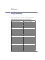
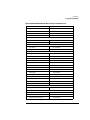
Language Compatibility
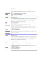
This section lists Agilent 83480A commands that are not used in the 86100A/B/C.
Agilent 83480A/54750A Commands Not Used in the Instrument (1 of 6)
Programming Commands/Queries
Replacement Commands/Queries
Common Commands
*LRN
SYSTEM:SETUP
Root Level Commands
:AER?
No replacement
:ERASe
No replacement
:HEEN
:AEEN
:MENU
No replacement
:MERGe
No replacement
:STORe:PMEMory1
No replacement
:TEER
No replacement
System Commands :SYSTem
:SYSTem:KEY
No replacement
Calibration Commands :CALibrate
1-36
:CALibrate:FRAMe:CANCel
:CALibrate:CANcel
:CALibrate:FRAMe:CONTinue
:CALibrate:CONTinue
:CALibrate:FRAMe:DATA
No replacement
:CALibrate:FRAMe:DONE?
:CALibrate:STATus?
:CALibrate:FRAMe:MEMory?
No replacement
:CALibrate:PLUGin:ACCuracy
:CALibrate:MODule:STATus
:CALibrate:PLUGin:CANCel
:CALibrate:CANcel
:CALibrate:PLUGin:CONTinue
:CALibrate:CONTinue
:CALibrate:PLUGin:DONE?
:CALibrate:STATus?
:CALibrate:PLUGin:MEMory?
No replacement
:CALibrate:PLUGin:OFFSet
:CALibrate:MODule:OFFSet
:CALibrate:PLUGin:OPOWer
:CALibrate:MODule:OPOWer
Introduction
Language Compatibility
Agilent 83480A/54750A Commands Not Used in the Instrument (2 of 6)
:CALibrate:PLUGin:OPTical
:CALibrate:MODule:OPTical
:CALibrate:PLUGin:OWAVelength
:CALibrate:MODule:OWAVelength
:CALibrate:PLUGin:TIME?
:CALibrate:MODule:TIME?
:CALibrate:PLUGin:VERTical
:CALibrate:MODule:VERtical
:CALibrate:PROBe
:CALibrate:PROBe CHANnel<N>
Channel Commands :CHANnel
:CHANnel<N>:AUTOscale
:AUToscale
:CHANnel<N>:SKEW
:CALibrate:SKEW
Disk Commands :DISK
:DISK:DATA?
No replacement
:DISK:FORMat
No replacement
Display Commands :DISPlay
:DISPlay:ASSign
No replacement
:DISPlay:CGRade
:SYSTem:MODE EYE
:DISPlay:CGRade?
:SYSTem:MODE?
:DISPlay:COLumn
:DISPlay:LABel
:DISPlay:DATA
:WAVeform:DATA
:DISPlay:DWAVeform
No replacement
:DISPlay:FORMat
No replacement
:DISPlay:INVerse
:DISPlay:LABel
:DISPlay:LINE
:DISPlay:LABel
:DISPlay:MASK
No replacement
:DISPlay:ROW
:DISPlay:LABel
:DISPlay:SOURce
No replacement
:DISPlay:STRing
:DISPlay:LABel
:DISPlay:TEXT
:DISPlay:LABel:DALL
FFT Commands :FFT
FFT is not available in the 86100A/B.
Function Commands :FUNCtion
:FUNCtion<N>:ADD
No replacement
:FUNCtion<N>:BWLimit
No replacement
:FUNCtion<N>:DIFFerentiate
No replacement
1-37
Introduction
Language Compatibility
Agilent 83480A/54750A Commands Not Used in the Instrument (3 of 6)
:FUNCtion<N>:DIVide
No replacement
:FUNCtion<N>:FFT
No replacement, FFT not available
:FUNCtion<N>:INTegrate
No replacement
:FUNCtion<N>:MULTiply
No replacement
:FUNCtion<N>:ONLY
:FUNCtion<N>:MAGNify
Hardcopy Commands :HARDcopy
:HARDcopy:ADDRess
:HARDcopy:DPRinte
:HARDcopy:BACKground
:HARDcopy:IMAGe INVert
:HARDcopy:BACKground?
No replacement
:HARDcopy:DESTination
No replacement
:HARDcopy:DEVice
No replacement
:HARDcopy:FFEed
No replacement
:HARDcopy:FILename
No replacement
:HARDcopy:LENGth
No replacement
:HARDcopy:MEDia
No replacement
Histogram Commands :HISTogram
:HISTogram:RRATe
:DISPlay:RRATe
:HISTogram:RUNTil
:ACQuire:RUNTil
:HISTogram:SCALe
:HISTogram:SCALe:SIZE
:HISTogram:SCALe:OFFSet
:HISTogram:SCALe:SIZE
:HISTogram:SCALe:RANGe
:HISTogram:SCALe:SIZE
:HISTogram:SCALe:SCALe
:HISTogram:SCALe:SIZE
:HISTogram:SCALe:TYPE
:HISTogram:SCALe:SIZE
Limit Test Commands :LTESt
1-38
:LTESt:SSCReen:DDISk:BACKground
:LTESt:SSCReen:IMAGe
:LTESt:SSCReen:DDISk:MEDia
No replacement
:LTESt:SSCReen:DDISk:PFORmat
No replacement
:LTESt:SSCReen:DPRinter:ADDRess
No replacement
:LTESt:SSCReen:DPRinter:BACKground
No replacement
:LTESt:SSCReen:DPRinter:MEDia
No replacement
:LTESt:SSCReen:DPRinter:PORT
No replacement
:LTESt:SSUMmary:ADDRess
No replacement
Introduction
Language Compatibility
Agilent 83480A/54750A Commands Not Used in the Instrument (4 of 6)
:LTESt:SSUMmary:MEDia
No replacement
:LTESt:SSUMmary:PFORmat
No replacement
:LTESt:SSUMmary:PORT
No replacement
Marker Commands :MARKer
:MARKer:CURSor?
No replacement. Use individual queries.
:MARKer:MEASurement:READout
No replacement
:MARKer:MODE
:MARKer:STATe
:MARKer:MODE?
No replacement
:MARKer:TDELta?
:MARKer:XDELta?
:MARKer:TSTArt
:MARKer:X1Position
:MARKer:TSTOp
:MARKer:X2Position
:MARKer:VDELta
:MARKer:YDELta
:MARKer:VSTArt
:MARKer:Y1Position
:MARKer:VSTOp
:MARKer:Y2Position
Mask Test Commands :MTESt
:MTESt:AMASk:CReate
No replacement
:MTESt:AMASk:SOURce
No replacement
:MTESt:AMASk:UNITs
No replacement
:MTESt:AMASk:XDELta
No replacement
:MTESt:AMASk:YDELta
No replacement
:MTESt:AMODe
No replacement
:MTESt:COUNt:FWAVeforms?
MTESt:COUNt:HITS? TOTal
:MTESt:FENable
No replacement
:MTESt:MASK:DEFine
No replacement a
:MTESt:POLYgon:DEFine
No replacement a
:MTESt:POLYgon:DELete
No replacement a
:MTESt:POLYgon:MOVE
No replacement a
:MTESt:RECall
:MTESt:LOAD
:MTESt:SAVE
No replacement
:MTESt:SSCReen:DDISk:BACKground
:MTESt:SSCReen:IMAGe
:MTESt:SSCReen:DDISk:MEDia
No replacement
:MTESt:SSCReen:DDISk:PFORmat
No replacement
1-39
Introduction
Language Compatibility
Agilent 83480A/54750A Commands Not Used in the Instrument (5 of 6)
:MTESt:SSCReen:DPRinter
No replacement
:MTESt:SSCReen:DPRinter:ADDRess
No replacement
:MTESt:SSCReen:DPRinter:BACKground
No replacement
:MTESt:SSCReen:DPRinter:MEDia
No replacement
:MTESt:SSCReen:DPRinter:PFORmat
No replacement
:MTESt:SSCReen:DPRinter:PORT
No replacement
:MTESt:SSUMmary:ADDRess
No replacement
:MTESt:SSUMmary:BACKground
No replacement
:MTESt:SSUMmary:MEDia
No replacement
:MTESt:SSUMmary:PFORmat
No replacement
:MTESt:SSUMmary:PORT
No replacement
Measure Commands :MEASure
:MEASure:CGRade:ERCalibrate
:MEASure:CGRade:ERFactor
No replacement
:MEASure:CGRade:QFACtor
:MEASure:CGRade:ESN
:MEASure:FFT
No replacement. FFT not available.
:MEASure:HISTogram:HITS
Query only
:MEASure:HISTogram:MEAN
Query only
:MEASure:HISTogram:MEDian
Query only
:MEASure:HISTogram:M1S
Query only
:MEASure:HISTogram:M2S
Query only
:MEASure:HISTogram:OFFSET?
No replacement
:MEASure:HISTogram:PEAK
Query only
:MEASure:HISTogram:PP
Query only
:MEASure:PREShoot
No replacement
:MEASure:STATistics
No replacement. Statistics always on.
:MEASure:TEDGe
Query only
:MEASure:VLOWer
No replacement
:MEASure:VMIDdle
No replacement
:MEASure:VTIMe
Query only
:MEASure:VUPPer
No replacement
Timebase Commands :TIMebase
1-40
:CALibrate:ERATio:STARt CHANnel<N>
Introduction
Language Compatibility
Agilent 83480A/54750A Commands Not Used in the Instrument (6 of 6)
:TIMebase:DELay
:TIMebase:POSition
:TIMebase:VIEW
No replacement
:TIMebase:WINDow:DELay
No replacement
:TIMebase:WINDow:POSition
No replacement
:TIMebase:WINDow:RANGe
No replacement
:TIMebase:WINDow:SCALe
No replacement
:TIMebase:WINDow:SOURce
No replacement
Trigger Commands :TRIGger
:TRIGger:SWEep
:TRIGger:SOURce FRUN
:TRIGger:SWEep?
:TRIGger:SOURce?
:TRIGger<N>:BWLimit
:TRIGger:BWLimit and :TRIGger:GATed
:TRIGger<N>:PROBe
:TRIGger:ATTenuation
Waveform Commands :WAVeform
a
:WAVeform:COMPlete
No replacement
:WAVeform:COUPling
No replacement
:WAVeform:VIEW?
No replacement
Refer to the Infiniium DCA Online Help to view information about defining custom masks.
1-41
Introduction
New and Revised Commands
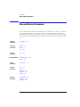
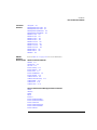
New and Revised Commands
This section lists all new and revised commands for the 86100C. Some of these commands are
new to software revision A.5.00 and some are new to software revision A.6.00. Each command listed is followed by the page number where the command is documented. For revision
A.6.00, changes to the TDR subsystem are significant enough to require a separate new chapter.
Common
Commands
*OPT? (Option) 3-7
Root Level
Commands
CDISplay 4-5
RUN 4-12
STOP 4-13
Acquire
Commands
LTESt
Disk Commands
SPARameter:SAVE
STORe 10-9
Display
Commands
JITTer:SHADe 11-5
Function
Commands
ADD 12-3
DIFF 12-3
HORizontal 12-4
MULTiply 12-6
PEELing 12-7
Measure
Commands
TDR:AVERage 18-33
TDR:MAX 18-33
TDR:MIN 18-33
1-42
6-3
10-8
Introduction
New and Revised Commands
S-Parameter
Commands
TDRSparam 19-3
MAGGraph:HORizontal:STARt 19-3
MAGGraph:HORizontal:SPAN 19-3
MAGGraph:VERTical:MAXimum 19-4
MAGGraph:VERTical:MINimum 19-4
MARKer:X1STate 19-4
MARKer:X2STate 19-4
MARKer:X1Source 19-4
MARKer:X2Source 19-5
MARKer:X1Position 19-5
MARKer:X2Position 19-5
MARKer:Y1Position? 19-5
MARKer:Y2Position? 19-6
MARKer:XDELta? 19-6
MARKer:YDELta? 19-6
VWINdow 19-6
TDR/TDT
Commands
(Revision A.6.00)
Refer to Table 22-1 on page 22-2 for a more information.
New Revision A.6.00 Commands
CONNect 22-4
DUT:DIRection 22-4
DUT:TYPE 22-4
RESPonse:DISPlay 22-6
RESPonse:RPLane? 22-7
RESPonse:TYPE 22-7
RESPonse:VAMPlitude? 22-7
RESPonse:VLOad? 22-9
STIMulus:EXTernal 22-9
STIMulus:EXTernal:POLarity 22-9
STIMulus:MODE 22-10
STIMulus:RATE 22-10
STIMulus:STATe 22-10
Revision A.5.00 Commands Not Supported In Revision A.6.00
DCALib
HPOLarity
NVALid
PRESet
RESPonse:
RESPonse:CALibrate:CANCel
RESPonse:CALibrate:CONTinue
RESPonse:HORizontal
RESPonse:HORizontal:POSition
RESPonse:HORizontal:RANGe
RESPonse:TDRDest
1-43
Introduction
Commands Unavailable in Jitter Mode
RESPonse:TDRTDT
RESPonse:TDTDest
STIMulus
Timebase
Commands
MPOSition 23-2
Commands Unavailable in Jitter Mode
This section describes the commands that can generate errors when controlling the instrument in Jitter mode. This can be due to the command or one of its arguments that are not
allowed in Jitter mode. Refer to the individual command reference for detailed information.
Refer to “New and Revised Commands” on page 1-42 for a list of commands that can be used
to control Jitter mode.
Waveform Files
Waveform and Color Grade/Gray Scale files cannot be saved or loaded in Jitter mode. The
commands listed below produce a "Settings conflict" error when executed in Jitter Mode.
DISK:STORe 10-9
When used with sources other than SETup and JDMemory.
STORe:WAVeform 4-14
ACQuire:SWAVeform 6-6
LTESt:SWAVeform 15-8
MTESt:SWAVeform 17-13
Waveform
Queries
Only jitter database waveforms may be set or queried in Jitter mode. Using the following command produces the error, "Signal or trigger source selection is not available".
:WAVeform:DATA 25-4
Waveform
Memory Load/
Store
Waveforms cannot be saved into waveform memories in Jitter mode. All waveform memories
are turned off when entering Jitter mode. The commands listed below produce a "Settings
conflict" error when executed in Jitter mode.
WMEMory<N>:LOAD 26-2
WMEMory<N>:SAVE 26-3
DISK:LOAD 10-3
When used with sources other than SETup and JDMemory.
1-44
Introduction
Commands Unavailable in Jitter Mode
WAveform
Memory Display
Waveform memories cannot be turned on in Jitter mode. The following command produces a
"Settings conflict" error when executed in Jitter mode.
WMEMory<N>:DISPlay 26-2
Waveform and
The Waveform and Color Grade/Gray Scale memories cannot be turned on in Jitter mode. The
Color Grade-Gray following command produces an "Illegal parameter value" error when executed in Jitter
Scale Memory
mode.
VIEW 4-15
When used with arguments other than JDMemory.
Timebase Scale
And Delay
Scale and position controls on the Horizontal setup dialog are disabled in Jitter Mode. The following commands produce a "Settings conflict" error when executed in Jitter Mode:
TIMebase:RANGe 23-4
TIMebase:SCALe 23-5
TIMebase:POSition 23-2
Channel Scale
And Offset
Channel scale and offset controls are disabled in Jitter mode. The following commands produce a "Settings conflict" error when executed in Jitter Mode.
CHANnel<N>:OFFSet 8-4
CHANnel<N>:RANGe 8-5
CHANnel<N>:SCALe 8-6
Acquisition
Settings
Acquisition (Averaging) controls are disabled in Jitter mode. The following commands produce a "Settings conflict" error when executed in Jitter mode.
ACQuire:AVERage 6-2
ACQuire:BEST 6-2
ACQuire:POINts 6-3
Histograms
Histograms are turned off when entering Jitter mode. The following commands produce a
"Control is set to default" error.
HISTogram:MODE
VIEW 4-15
Software
Skewing of
Channels
14-3
All skew adjustments are disabled in jitter mode. The following commands produce a "Settings conflict" error when executed in Jitter mode.
CALibrate:SKEW 7-9
CALibrate:SKEW:AUTO 7-10
1-45
Introduction
Error Messages
Error Messages
This chapter describes the error messages and how they are generated. The possible causes
for the generation of the error messages are also listed in Table 1-10 on page 1-47.
Error Queue
As errors are detected, they are placed in an error queue. This queue is first in, first out. If
the error queue overflows, the last error in the queue is replaced with error –350, “Queue
overflow.” Anytime the error queue overflows, the oldest errors remain in the queue, and the
most recent error is discarded. The length of the instrument's error queue is 30 (29 positions
for the error messages, and 1 position for the “Queue overflow” message). Reading an error
from the head of the queue removes that error from the queue, and opens a position at the
tail of the queue for a new error. When all errors have been read from the queue, subsequent
error queries return 0, “No error.”
The error queue is cleared when any of the following occur:
•
•
•
•
Error Numbers
The error numbers are grouped according to the type of error that is detected.
•
•
•
•
•
•
Command Error
the instrument is powered up,
a *CLS command is sent,
the last item from the queue is read, or
the instrument is switched from talk only to addressed mode on the front panel.
+0 indicates no errors were detected.
–100 to –199 indicates a command error was detected.
–200 to –299 indicates an execution error was detected.
–300 to –399 indicates a device-specific error was detected.
–400 to –499 indicates a query error was detected.
+1 to +32767 indicates an instrument-specific error has been detected.
Refer to the Agilent 86100A/B/C online Help for instrument specific errors.
An error number in the range –100 to –199 indicates that an IEEE 488.2 syntax error has
been detected by the instrument's parser. The occurrence of any error in this class sets the
command error bit (bit 5) in the event status register and indicates that one of the following
events occurred:
• An IEEE 488.2 syntax error was detected by the parser. That is, a controller-to-instrument
message was received that is in violation of the IEEE 488.2 standard. This may be a data element that violates the instrument's listening formats, or a data type that is unacceptable to the
instrument.
• An unrecognized header was received. Unrecognized headers include incorrect instrument-
1-46
Introduction
Error Messages
specific headers and incorrect or unimplemented IEEE 488.2 common commands.
• A Group Execute Trigger (GET) was entered into the input buffer inside of an IEEE 488.2 program message.
Events that generate command errors do not generate execution errors, instrument-specific
errors, or query errors.
Execution Error
An error number in the range –200 to –299 indicates that an error was detected by the instrument's execution control block. The occurrence of any error in this class causes the execution error bit (bit 4) in the event status register to be set. It also indicates that one of the
following events occurred:
• The program data following a header is outside the legal input range or is inconsistent with the
instrument's capabilities.
• A valid program message could not be properly executed due to some instrument condition.
Execution errors are reported by the instrument after expressions are evaluated and rounding operations are completed. For example, rounding a numeric data element will not be
reported as an execution error. Events that generate execution errors do not generate command errors, instrument specific errors, or query errors.
Device- or
InstrumentSpecific Error
An error number in the range of –300 to –399 or +1 to +32767 indicates that the instrument
has detected an error caused by an instrument operation that did not properly complete. This
may be due to an abnormal hardware or firmware condition. For example, this error may be
generated by a self-test response error, or a full error queue. The occurrence of any error in
this class causes the instrument-specific error bit (bit 3) in the event status register to be set.
Query Error
An error number in the range –400 to –499 indicates that the output queue control of the
instrument has detected a problem with the message exchange protocol. An occurrence of
any error in this class causes the query error bit (bit 2) in the event status register to be set.
An occurrence of an error also means one of the following is true:
• An attempt is being made to read data from the output queue when no output is either present
or pending.
• Data in the output queue has been lost.
Table 1-10. Error Messages Returned by Instrument Parser (1 of 4)
0
No error
The error queue is empty. Every error in the queue has been read (SYSTEM:ERROR?
query) or the queue was cleared by power-up or *CLS.
-100
Command error
This is the generic syntax error used if the instrument cannot detect more specific errors.
-101
Invalid character
A syntactic element contains a character that is invalid for that type.
-102
Syntax error
An unrecognized command or data type was encountered.
-103
Invalid separator
The parser was expecting a separator and encountered an illegal character.
1-47
Introduction
Error Messages
Table 1-10. Error Messages Returned by Instrument Parser (2 of 4)
-104
Data type error
The parser recognized a data element different than one allowed. For example, numeric
or string data was expected but block data was received.
-105
GET not allowed
A Group Execute Trigger was received within a program message.
-108
Parameter not allowed
More parameters were received than expected for the header.
-109
Missing parameter
Fewer parameters were received than required for the header.
-112
Program mnemonic too long
The header or character data element contains more than twelve characters.
-113
Undefined header
The header is syntactically correct, but it is undefined for the instrument. For example,
*XYZ is not defined for the instrument.
-121
Invalid character in number
An invalid character for the data type being parsed was encountered. For example, a “9”
in octal data.
-123
Numeric overflow
Number is too large or too small to be represented internally.
-124
Too many digits
The mantissa of a decimal numeric data element contained more than 255 digits
excluding leading zeros.
-128
Numeric data not allowed
A legal numeric data element was received, but the instrument does not accept one in
this position for the header.
-131
Invalid suffix
The suffix does not follow the syntax described in IEEE 488.2 or the suffix is inappropriate
for the instrument.
-138
Suffix not allowed
A suffix was encountered after a numeric element that does not allow suffixes.
-141
Invalid character data
Either the character data element contains an invalid character or the particular element
received is not valid for the header.
-144
Character data too long
-148
Character data not allowed
A legal character data element was encountered where prohibited by the instrument.
-150
String data error
This error can be generated when parsing a string data element. This particular error
message is used if the instrument cannot detect a more specific error.
-151
Invalid string data
A string data element was expected, but was invalid for some reason. For example, an
END message was received before the terminal quote character.
-158
String data not allowed
A string data element was encountered but was not allowed by the instrument at this
point in parsing.
-160
Block data error
This error can be generated when parsing a block data element. This particular error
message is used if the instrument cannot detect a more specific error.
-161
Invalid block data
-168
Block data not allowed
A legal block data element was encountered but was not allowed by the instrument at
this point in parsing.
-170
Expression error
This error can be generated when parsing an expression data element. It is used if the
instrument cannot detect a more specific error.
-171
Invalid expression
-178
Expression data not allowed
1-48
Expression data was encountered but was not allowed by the instrument at this point in
parsing.
Introduction
Error Messages
Table 1-10. Error Messages Returned by Instrument Parser (3 of 4)
-200
Execution error
This is a generic syntax error which is used if the instrument cannot detect more specific
errors.
-220
Parameter error
Indicates that a program data element related error occurred.
-221
Settings conflict
Indicates that a legal program data element was parsed but could not be executed due to
the current device state.
-222
Data out of range
Indicates that a legal program data element was parsed but could not be executed
because the interpreted value is outside the legal range defined by the instrument.
-223
Too much data
Indicates that a legal program data element of block, expression, or string type was
received that contained more data than the instrument could handle due to memory or
related instrument-specific requirements.
-224
Illegal parameter value
Used where exact value, from a list of possibles, was expected.
-225
Out of memory
The device has insufficient memory to perform the requested operation.
-231
Data questionable
Indicates that measurement accuracy is suspect.
-240
Hardware error
Indicates that a legal program command or query could not be executed because of a
hardware problem in the device.
-241
Hardware missing
Indicates that a legal program command or query could not be executed because of
missing device hardware; for example, an option was not installed, or current module
does not have hardware to support command or query. Definition of what constitutes
missing hardware is completely device-specific or module specific.
-250
Mass storage error
Indicates that a mass storage error occurred.
-251
Missing mass storage
Indicates that a legal program command or query could not be executed because of
missing mass storage; for example, an option that was not installed.
-252
Missing media
Indicates that a legal program command or query could not be executed because of a
missing media; for example, no disk.
-253
Corrupt media
Indicates that a legal program command or query could not be executed because of
corrupt media; for example, bad disk or wrong format.
-254
Media full
Indicates that a legal program command or query could not be executed because the
media was full; for example, there is no room on the disk.
-255
Directory full
Indicates that a legal program command or query could not be executed because the
media directory was full.
-256
File name not found
Indicates that a legal program command or query could not be executed because the file
name on the device media was not found; for example, an attempt was made to read or
copy a nonexistent file.
-257
File name error
Indicates that a legal program command or query could not be executed because the file
name on the device media was in error; for example, an attempt was made to copy to a
duplicate file name.
-258
Media protected
Indicates that a legal program command or query could not be executed because the
media was protected; for example, the write-protect tab on a disk was present.
-300
Service specific error
1-49
Introduction
Error Messages
Table 1-10. Error Messages Returned by Instrument Parser (4 of 4)
-310
System error
Indicates that a system error occurred.
-340
Calibration failed
Indicates that a calibration has failed.
-350
Queue overflow
Indicates that there is no room in the error queue and an error occurred but was not
recorded.
-400
Query error
This is the generic query error.
-410
Query INTERRUPTED
-420
Query UNTERMINATED
-430
Query DEADLOCKED
-440
Query UNTERMINATED
after indefinite response
1-50
2
Sample C Programs 2-3
init.c - Initialization 2-3
init.c - Global Definitions and Main Program 2-4
init.c - Initializing the Analyzer 2-4
init.c - Acquiring Data 2-5
init.c - Making Automatic Measurements 2-6
init.c - Error Checking 2-7
init.c - Transferring Data to the PC 2-9
init.c - Converting Waveform Data 2-10
init.c - Storing Waveform Time and Voltage Information 2-11
gen_srq.c - Generating a Service Request 2-11
Initializing the Analyzer 2-12
Setting Up a Service Request 2-13
Generating a Service Request 2-14
Listings of the Sample Programs 2-15
hpib_decl.h Sample Program 2-15
init.c Sample Program 2-17
gen_srq.c Sample Program 2-23
srq.c Sample Program 2-25
learnstr.c Sample Program 2-26
sicl_IO.c Sample Program 2-29
natl_IO.c Sample Program 2-32
multidatabase.c Sample Program 2-35
init.bas Sample Program 2-38
srq.bas Sample Program 2-44
lrn_str.bas Sample Program 2-47
Sample Programs
Sample Programs
Sample Programs
Each program in this chapter demonstrates specific sets of instructions. This chapter shows
you some of those functions, and describes the commands being executed. The sample program listings are included at the end of this chapter. Both C and BASIC examples are
included. The header file is:
hpibdecl.h
The C examples include:
•
•
•
•
•
•
•
init.c
gen_srq.c
srq.c
learnstr.c
sicl_IO.c
natl_IO.c
multidatabase.c
The BASIC examples include:
• init.bas
• srq.bas
• lrn_str.bas
This chapter includes segments of both the C and BASIC sample programs. Each program
includes the basic functions of initializing the interface and analyzer, capturing the data, and
analyzing the data. In general, both the C and BASIC sample programs typically contain the
following fundamental segments:
Segment
Description
main program
Defines global variables and constants, specifies include files, and
calls various functions.
initialize
Initializes the GPIB and analyzer, and sets up the analyzer and the ACQuire subsystem.
acquire_data
Digitizes the waveform to capture data.
auto_measurements
Performs simple parametric measurements.
transfer_data
Brings waveform data and voltage/timing information (the preamble) into the computer.
2-2
Sample Programs
Sample C Programs
Sample C Programs
Segments of the sample programs “init.c” and “gen_srq.c” are shown and described in this
chapter.
init.c - Initialization
/*
init. c */
/*
Command Order Example. This program demonstrates the order of commands suggested for operation of the analyzer via GPIB.
This program initializes the scope, acquires data, performs automatic measurements, and transfers and stores the data on the PC
as time/voltage pairs in a comma-separated file format useful for spreadsheet applications. It assumes a SICL INTERFACE exists
as 'hpib7' and an Agilent 86100 analyzer at address 7. It also requires the cal signal attached to Channel 1.
See the README file on the demo disk for development and linking information.
*/
# include <stdio.h>
# include <stdlib.h>
# include "hpibdecl.h"
/* location of: printf ( ) */
/* location of: atof(), atoi ( ) */
/* prototypes, global declarations, constants */
void initialize ( );
void acquire_data ( );
void auto_measurements ( );
void transfer_data ( );
void convert_data ( );
void store_csv ( );
/* initialize the scope */
/* digitize signal */
/* perform built-in automatic measurements */
/* transfers waveform data from scope to PC */
/* converts data to time/voltage values */
/* stores time/voltage pairs to comma-separated
/* variable file format */
The include statements start the program. The file “hpibdecl.h” includes prototypes and declarations that are necessary for the analyzer sample programs.
This segment of the sample program defines the functions, in order, that are used to initialize
the scope, digitize the data, perform measurements, transfer data from the scope to the PC,
convert the digitized data to time and voltage pairs, and store the converted data in commaseparated variable file format.
See the following descriptions of the program segments.
2-3
Sample Programs
Sample C Programs
init.c - Global Definitions and Main Program
/* GLOBALS */
int count;
double xorg,xref,xinc;
double yorg,yref,yinc;
int Acquired_length;
char data[MAX_LENGTH];
double time_value[MAX_LENGTH];
double volts[MAX_LENGTH];
/* values necessary for conversion of data */
/* data buffer */
/* time value of data */
/* voltage value of data */
void main( void )
{
/* initialize interface and device sessions */
/* note: routine found in sicl_IO.c or natl_IO.c */
init_IO ( );
initialize ( );
acquire_data ( );
auto_measurements ( );
transfer_data ( );
convert_data ( );
store_csv ( );
close_IO ( );
/* initialize the scope and interface and set up SRQ */
/* capture the data */
/* perform automated measurements on acquired data */
/* transfer waveform data to the PC from scope */
/* convert data to time/voltage pairs */
/* store the time/voltage pairs as csv file */
/* close interface and device sessions */
/* note: routine found in sicl_IO.c or natl_IO.c */
} /* end main ( ) */
The init_IO routine initializes the analyzer and interface so that the scope can capture data
and perform measurements on the data. At the start of the program, global symbols are
defined which will be used to store and convert the digitized data to time and voltage values.
init.c - Initializing the Analyzer
/*
* Function name: initialize
* Parameters: none
* Return value: none
* Description: This routine initializes the analyzer for proper
* acquisition of data. The instrument is reset to a known state and the
* interface is cleared. System headers are turned off to allow faster
* throughput and immediate access to the data values requested by queries.
* The analyzer time base, channel, and trigger subsystems are then
* configured. Finally, the acquisition subsystem is initialized.
*/
void initialize ( )
{
write_IO ("*RST");
/* reset scope - initialize to known state */
2-4
Sample Programs
Sample C Programs
write_IO ("*CLS");
/* clear status registers and output queue */
write_IO (":SYSTem:HEADer OFF");
/* turn off system headers */
/* initialize time base parameters to center reference, */
/* 2 ms full-scale (200 us/div), and 20 us delay */
write_IO (":TIMebase:REFerence CENTer;RANGe 2e-3;POSition 20e-6");
/* initialize Channel1 1.6V full-scale (200 mv/div); offset -400mv */
write_IO (":CHANnel1:RANGe 1.6;OFFSet -400e-3");
/* initialize trigger info: channel1 signal on positive slope at 300mv */
write_IO (":TRIGger:SOURce FPANel;SLOPe POSitive");
write_IO (":TRIGger:LEVel-0.40");
/* initialize acquisition subsystem */
/* Real time acquisition - no averaging; record length 4096 */
write_IO (":ACQuire:AVERage OFF;POINts 4096");
} /* end initialize ( ) */
init.c - Acquiring Data
/*
* Function name: acquire_data
* Parameters: none
* Return value: none
* Description: This routine acquires data according to the current
* instrument settings.
*/
void acquire_data ( )
{
/*
* The root level :DIGitize command is recommended for acquisition of new
* data when averaging is used. It will initialize data buffers, acquire new data, and ensure that
* acquisition criteria are met before acquisition of data is stopped. The
* captured data is then available for measurements, storage, or transfer
* to a PC. Note that the display is automatically turned off by the
* :DIGitize command and must be turned on to view the captured data.
*/
write_IO (":DIGitize CHANnel1");
write_IO (":CHANnel1:DISPlay ON");
/* turn on channel 1 display which is */
/* turned off by the :DIGitize command */
} /* end acquire_data ( ) */
2-5
Sample Programs
Sample C Programs
init.c - Making Automatic Measurements
/*
* Function name: auto_measurements
* Parameters: none
* Return value: none
* Description: This routine performs automatic measurements of volts
* peak-to-peak and period on the acquired data. It also demonstrates
* two methods of error detection when using automatic measurements.
*/
void auto_measurements ( )
{
float period, vpp;
unsigned char vpp_str[16];
unsigned char period_str[16];
int bytes_read;
/*
* Error checking on automatic measurements can be done using one of two methods.
* The first method requires that you turn on results in the Measurements
* subsystem using the command :MEASure:SEND ON. When this is on, the analyzer
* will return the measurement and a result indicator. The result flag is zero
* if the measurement was successfully completed, otherwise a non-zero value is
* returned which indicates why the measurement failed. See the Programmer's Manual
* for descriptions of result indicators.
*
* The second method simply requires that you check the return value of the
* measurement. Any measurement not made successfully will return with the value
* +9.999E37. This could indicate that either the measurement was unable to be
* performed, or that insufficient waveform data was available to make the
* measurement.
*/
/*
* METHOD ONE - turn on results to indicate whether the measurement completed
* successfully. Note that this requires transmission of extra data from the scope.
*/
write_IO (":MEASure:SEND ON");
/* turn results on */
write_IO (":MEASure:VPP? CHANnel1");
/* query -- volts peak-to-peak channel 1*/
bytes_read = read_IO(vpp_str,16L);
/* read in value and result flag */
if (vpp_str[bytes_read-2] != '0')
printf ("Automated vpp measurement error with result %c\n",
vpp_str [bytes_read-2]);
else
printf ("VPP is %f\n", (float) atof (vpp_str));
write_IO (":MEASure:PERiod? CHANnel1");
/* period channel 1 */
bytes_read = read_IO (period_str,16L);
/* read in value and result flag */
if period_str[bytes_read-2] != '0')
printf ("Automated period measurement error with result %c\n",
2-6
Sample Programs
Sample C Programs
period_str [bytes_read-2]);
else
printf ("Period is %f\n",(float)atof (period_str));
/*
* METHOD TWO - perform automated measurements and error checking with
* :MEAS:RESULTS OFF
*/
period = (float) 0;
vpp = (float) 0;
/* turn off results */
write_IO (":MEASure:SEND OFF");
write_IO (":MEASure:PERiod? CHANnel1");
bytes_read = read_IO (period_str,16L);
/*period 1 */
/* read in value and result flag */
period = (float) atof (period_str);
if (period > 9.99e37 )
printf ("\nPeriod could not be measured.\n");
else
printf ("\nThe period of channel 1 is %f seconds.\n", period );
write_IO (":MEASure:VPP? CHANnel1");
bytes_read = read_IO ( vpp_str,16L );
vpp = (float) atof (vpp_str);
if ( vpp > 9.99e37 )
printf ("Peak-to-peak voltage could not be measured.\n");
else
printf ("The voltage peak-to-peak is %f volts.\n", vpp );
} /* end auto_measurements () */
init.c - Error Checking
/* Error checking on automatic measurements can be done using one of two methods.
* The first method requires that you turn on results in the Measurements
* subsystem using the command :MEASure:SEND ON. When this is on, the analyzer
* will return the measurement and a result indicator. The result flag is zero
* if the measurement was successfully completed, otherwise a non-zero value is
* returned which indicates why the measurement failed. See the Programmer's Manual
* for descriptions of result indicators.
*
*
*
*
*
The second method simply requires that you check the return value of the
measurement. Any measurement not made successfully will return with the value
+9.999E37. This could indicate that either the measurement was unable to be
performed, or that insufficient waveform data was available to make the
measurement.
2-7
Sample Programs
Sample C Programs
* METHOD ONE - turn on results to indicate whether the measurement completed
* successfully. Note that this requires transmission of extra data from the scope.
*/
write_IO (":MEASure:SEND ON");
/* turn results on */
/* query -- volts peak-to-peak channel 1*/
write_IO (":MEASure:VPP? CHANnel1");
bytes_read = read_IO(vpp_str,16L);
/* read in value and result flag */
if (vpp_str[bytes_read-2] != '0')
printf ("Automated vpp measurement error with result %c\n",
vpp_str[bytes_read-2]);
else
printf ("VPP is %f\n",(float)atof(vpp_str));
write_IO (":MEASure:PERiod? CHANnel1");
bytes_read = read_IO(period_str,16L);
/* period channel 1 */
/* read in value and result flag */
if period_str[bytes_read-2] != '0')
printf ("Automated period measurement error with result %c\n",
period_str[bytes_read-2]);
else
printf ("Period is %f\n",(float)atof (period_str));
/*
* METHOD TWO - perform automated measurements and error checking with
* :MEAS:RESULTS OFF.
*/
period = (float) 0;
vpp = (float) 0;
/* turn off results */
write_IO (":MEASure:SEND OFF");
write_IO (":MEASure:PERiod? CHANnel1");
bytes_read = read_IO (period_str,16L);
period = (float) atof (period_str);
if ( period > 9.99e37 )
printf ("\nPeriod could not be measured.\n");
else
printf ("\nThe period of channel 1 is %f seconds.\n", period );
write_IO (":MEASure:VPP? CHANnel1");
bytes_read = read_IO ( vpp_str,16L );
vpp = (float) atof (vpp_str);
if ( vpp > 9.99e37 )
printf ("Peak-to-peak voltage could not be measured.\n");
else
printf ("The voltage peak-to-peak is %f volts.\n", vpp );
} /* end auto_measurements() */
2-8
/* period channel 1 */
/* read in value and result flag */
Sample Programs
Sample C Programs
init.c - Transferring Data to the PC
/*
* Function name: transfer_data
* Parameters: none
* Return value: none
* Description: This routine transfers the waveform conversion factors and
* waveform data to the PC.
*/
void transfer_data ( )
{
int header_length;
char header_str[8];
char term;
char xinc_str[32],xorg_str[32],xref_str[32];
char yinc_str[32],yref_str[32],yorg_str[32];
int bytes_read;
/* waveform data source channel 1 */
write_IO (":WAVeform:SOURce CHANnel1");
/* setup transfer format */
write_IO (":WAVeform:FORMat BYTE");
/* request values to allow interpretation of raw data */
write_IO (":WAVeform:XINCrement?");
bytes_read = read_IO (xinc_str,32L);
xinc = atof (xinc_str);
write_IO (":WAVeform:XORigin?");
bytes_read = read_IO (xorg_str,32L);
xorg = atof (xorg_str);
write_IO (":WAVeform:XREFerence?");
bytes_read = read_IO (xref_str,32L);
xref = atof (xref_str);
write_IO (":WAVeform:YINCrement?");
bytes_read = read_IO (yinc_str,32L);
yinc = atof (yinc_str);
write_IO (":WAVeform:YORigin?");
bytes_read = read_IO (yorg_str,32L);
yorg = atof (yorg_str);
write_IO (":WAVeform:YREFerence?");
bytes_read = read_IO (yref_str,32L);
yref = atof (yref_str);
write_IO (":WAVeform:DATA?");
while (data[0] != ‘#’)
bytes_read = read_IO (data,1L);
bytes_read = read_IO (header_str,1L);
/* request waveform data */
/* find the # character */
/* input byte counter */
2-9
Sample Programs
Sample C Programs
header_length = atoi (header_str);
/* read number of points - value in bytes */
bytes_read = read_IO (header_str,(long)header_length);
Acquired_length = atoi (header_str);
/* number of bytes */
bytes_read = read_IO (data,Acquired_length);
bytes_read = read_IO (&term,1L);
/* input waveform data */
/* input termination character */
} /* end transfer_data () */
An example header resembles the following when the information is stripped off:
#510225
The left-most “5” defines the number of digits that follow (10225). The number “10225” is the
number of points in the waveform. The information is stripped off of the header to get the
number of data bytes that need to be read from the analyzer.
init.c - Converting Waveform Data
/*
* Function name: convert_data
* Parameters: none
* Return value: none
* Description: This routine converts the waveform data to time/voltage
* information using the values that describe the waveform. These values are
* stored in global arrays for use by other routines.
*/
void convert_data ( )
{
int i;
for (i = 0; i < Acquired_length; i++)
{
time_value[i] = ((i - xref) * xinc) + xorg;/* calculate time info */
volts[i] = ((data[i] - yref) * yinc) + yorg;/* calculate volt info */
}
} /* end convert_data ( ) */
The data values are returned as digitized samples (sometimes called quantization levels or qlevels). These data values must be converted into voltage and time values.
2-10
Sample Programs
Sample C Programs
init.c - Storing Waveform Time and Voltage Information
/*
* Function name: store_csv
* Parameters: none
* Return value: none
* Description: This routine stores the time and voltage information about
* the waveform as time/voltage pairs in a comma-separated variable file
* format.
*/
void store_csv ( )
{
FILE *fp;
int i;
fp = fopen ("pairs.csv","wb");
/* open file in binary mode - clear file */
/* if already exists */
if (fp != NULL)
{
for (i = 0; i < Acquired_length; i++)
{
/* write time,volt pairs to file */
fprintf ( fp,"%e,%lf\n",time_value[i],volts[i]);
}
fclose ( fp );
/* close file */
}
else
printf ("Unable to open file 'pairs.csv'\n");
} /* end store_csv ( ) */
The time and voltage information of the waveform is stored in integer format, with the time
stored first, followed by a comma, and the voltage stored second.
gen_srq.c - Generating a Service Request
Segments of the sample C program “gen_srq.c” show how
to initialize the interface
and analyzer, and generate a service request.
Two include statements start the “gen_srq.c” program. The file “stdio.h” defines the standard
location of the printf routine, and is needed whenever input or output functions are used.
The file “hpibdecl.h” includes necessary prototypes and declarations for the analyzers sample
programs. The path of these files must specify the disk drive and directory where the
“include” files reside.
/* gen_srq.c */
/*
2-11
Sample Programs
Sample C Programs
* This example program initializes the Agilent 86100 scope, runs an autoscale,
* then generates and responds to a Service Request from the scope. The program
* assumes an Agilent 86100 at address 7, an interface card at interface select code 7,
* and a signal source attached to channel 1.
*/
#include <stdio.h>
#include "hpibdecl.h"
/* location of: printf ( ) */
void initialize ( );
void setup_SRQ ( );
void create_SRQ ( );
void main ( void )
{
init_IO ( );
initialize ( );
setup_SRQ ( );
create_SRQ ( );
close_IO ( );
/* initialize interface and device sessions */
/* initialize the scope and interface */
/* enable SRQs on scope and set up SRQ handler */
/* generate SRQ */
/* close interface and device sessions */
} /* end main ( ) */
The routine “init_IO” contains three subroutines that initialize the analyzer and interface, and
sets up and generate a service request. The following segment describes the initialize subroutine.
Initializing the Analyzer
The following function is demonstrated in the “gen_srq.c” sample program.
/*
* Function name: initialize
* Parameters: none
* Return value: none
* Description: This routine initializes the analyzer for proper acquisition
* of data. The instrument is reset to a known state and the interface is
* cleared. System headers are turned off to allow faster throughput and
* immediate access to the data values requested by queries. The analyzer
* performs an autoscale to acquire waveform data.
*/
void initialize ( )
{
write_IO ("*RST");
/* reset scope - initialize to known state */
write_IO ("*CLS");
/* clear status registers and output queue */
write_IO (":SYSTem:HEADer OFF");/* turn off system headers */
write_IO (":AUToscale");
/* perform autoscale */
} /* end initialize ( ) */
2-12
Sample Programs
Sample C Programs
The *RST command is a common command that resets the analyzer to a known default configuration. Using this command ensures that the analyzer is in a known state before you configure it. *RST ensures very consistent and repeatable results. Without *RST, a program may run
one time, but it may give different results in following runs if the analyzer is configured differently. For example, if the trigger mode is normally set to edge, the program may function
properly. But, if someone puts the analyzer in the advanced TV trigger mode from the front
panel, the program may read measurement results that are totally incorrect. So, *RST defaults
the scope to a set configuration so that the program can proceed from the same state each
time. The *CLS command clears the status registers and the output queue. AUToscale finds and
displays all signals that are attached to the analyzer. You should program the analyzer’s time
base, channel, and trigger for the specific measurement to be made, as you would do from the
front panel, and use whatever other commands are needed to configure the analyzer for the
desired measurement.
Setting Up a Service Request
The following code segment shows how to generate a service request. The following function
is demonstrated in the “gen_srq.c” sample program.
/*
* Function name: setup_SRQ
* Parameters: none
* Return value: none
* Description: This routine initializes the device to generate Service Requests. It
* sets the Service Request Enable Register Event Status Bit and the Standard
* Event Status Enable Register to allow SRQs on Command, Execution, Device
* Dependent, or Query errors.
*/
void setup_SRQ ( )
{
/* Enable Service Request Enable Register - Event Status Bit */
write_IO ("*SRE 32");
/* Enable Standard Event Status Enable Register */
/* enable Command Error - bit 5 - value 32 */
/* Query Error - bit 2 - value 4 */
write_IO ("*ESE 36");
} /* end setup_SRQ ( ) */
2-13
Sample Programs
Sample C Programs
Generating a Service Request
The following function is demonstrated in the “gen_srq.c” sample program.
/*
* Function name: create_SRQ
* Parameters: none
* Return value: none
* Description: This routine sends two illegal commands to the scope which will
* generate an SRQ and will place two error strings in the error queue. The scope
* ID is requested to allow time for the SRQ to be generated. The ID string
* will contain a leading character which is the response placed in the output
* queue by the interrupted query.
*/
void create_SRQ ( )
{
char buf [256] = { 0 }; //read buffer for id string
int bytes_read = 0;
int srq_asserted;
/* Generate query error (interrupted query)*/
/* send legal query followed by another command other than a read query response */
write_IO (":CHANnel2:DISPlay?");
write_IO (":CHANnel2:DISPlay OFF");
/* Generate command error - send illegal header */
write_IO (":CHANnel:DISPlay OFF");
/* get instrument ID - allow time for SRQ to set */
write_IO ("*IDN?");
bytes_read = read_IO (buf,256L);
/* add NULL to end of string */
buf [bytes_read] = '\0';
printf ( "%s\n", buf);
srq_asserted = check_SRQ ( );
if ( srq_asserted )
srq_handler ( );
} /* end create_SRQ ( ) */
2-14
Sample Programs
Listings of the Sample Programs
Listings of the Sample Programs
Listings of the C sample programs in this section include:
•
•
•
•
•
•
•
hpibdecl.h
init.c
gen_srq.c
srq.c
learnstr.c
sicl_IO.c
natl_IO.c
Listings of the BASIC sample programs in this section include:
• init.bas
• srq.bas
• lrn_str.bas
hpib_decl.h Sample Program
/* hpibdecl.h */
/*
* This file includes necessary prototypes and declarations for
* the example programs for the Agilent 86100*/
*/
/*
* User must indicate which GPIB card (Agilent or National) is being used.
* Also, if using a National card, indicate which version of windows
* (WIN31 or WIN95) is being used.
*/
#define AGILENT
/* #define NATL */
/* Uncomment if using AGILENT interface card */
/* #define WIN31 */
#define WIN95
/* For National card ONLY - select windows version */
2-15
Sample Programs
Listings of the Sample Programs
#ifdef AGILENT
#include <sicl.h>
#else
#ifdef WIN95
#include <windows.h>
#include <decl-32.h>
#else
#include <windecl.h>
#endif
#endif
/* include file for Windows 95 */
/* include file for Windows 3.1 */
#define CME 32
#define EXE 16
#define DDE 8
#define QYE 4
#define SRQ_BIT 64
#define MAX_LRNSTR 14000
#define MAX_LENGTH 4096
#define MAX_INT 4192
#ifdef AGILENT
#define DEVICE_ADDR "hpib7,7"
#define INTERFACE "hpib7"
#else
#define INTERFACE "hpib0"
#define board_index 0
#define prim_addr 7
#define second_addr 0
#define timeout 13
#define eoi_mode 1
#define eos_mode 0
#endif
#define TRUE 1
#define FALSE 0
/* GLOBALS */
#ifdef AGILENT
INST bus;
INST scope;
#else
int bus;
int scope;
#endif
/* GPIB prototypes */
void init_IO ( );
void write_IO ( void* );
void write_lrnstr ( void*, long );
int read_IO ( void*, unsigned long );
int check_SRQ ( );
2-16
Sample Programs
Listings of the Sample Programs
unsigned char read_status ( );
void close_IO ( );
void hpiberr ( );
void srq_handler ( );
init.c Sample Program
/* init. c */
/*
* Command Order Example. This program demonstrates the order of commands
* suggested for operation of the Agilent 86100 analyzer via GPIB.
* This program initializes the scope, acquires data, performs
* automatic measurements, and transfers and stores the data on the
* PC as time/voltage pairs in a comma-separated file format useful
* for spreadsheet applications. It assumes a SICL INTERFACE exists
* as 'gpib7' and an Agilent 86100 analyzer at address 7.
* It also requires the cal signal attached to Channel 1.
*
* See the README file on the demo disk for development and linking information.
*/
#include <stdio.h>
#include <stdlib.h>
#include "hpibdecl.h"
/* location of: printf ( ) */
/* location of: atof(), atoi ( ) */
/* prototypes, global declarations, constants */
void initialize ( );
void acquire_data ( );
void auto_measurements ( );
void transfer_data ( );
void convert_data ( );
void store_csv ( );
/* initialize the scope */
/* digitize signal */
/* perform built-in automatic measurements */
/* transfers waveform data from scope to PC */
/* converts data to time/voltage values */
/* stores time/voltage pairs to comma-separated variable file format */
/* GLOBALS */
int count;
double xorg,xref,xinc;
/* values necessary for conversion of data */
double yorg,yref,yinc;
int Acquired_length;
char data [MAX_LENGTH];
/* data buffer */
double time_value [MAX_LENGTH];/* time value of data */
double volts [MAX_LENGTH];
/* voltage value of data */
void main( void )
{
/* initialize interface and device sessions */
/* note: routine found in sicl_IO.c or natl_IO.c */
init_IO ( );
initialize ( );
/* initialize the scope and interface and set up SRQ */
2-17
Sample Programs
Listings of the Sample Programs
acquire_data ( );
auto_measurements ( );
transfer_data ( );
convert_data ( );
store_csv ( );
close_IO ( );
/* capture the data */
/* perform automated measurements on acquired data */
/* transfer waveform data to the PC from scope */
/* convert data to time/voltage pairs */
/* store the time/voltage pairs as csv file */
/* close interface and device sessions */
/* note: routine found in sicl_IO.c or natl_IO.c */
} /* end main ( ) */
/*
* Function name: initialize
* Parameters: none
* Return value: none
* Description: This routine initializes the analyzer for proper
* acquisition of data. The instrument is reset to a known state and the
* interface is cleared. System headers are turned off to allow faster
* throughput and immediate access to the data values requested by queries.
* The analyzer time base, channel, and trigger subsystems are then
* configured. Finally, the acquisition subsystem is initialized.
*/
void initialize ( )
{
write_IO ("*RST");
write_IO ("*CLS");
/* reset scope - initialize to known state */
/* clear status registers and output queue */
write_IO (":SYSTem:HEADer OFF"); /* turn off system headers */
/* initialize time base parameters to center reference, 2 ms full-scale (200 us/div), and 20 us delay */
write_IO (":TIMebase:REFerence CENTer;RANGe 2e-3;POSition 20e-6");
/* initialize Channel1 1.6V full-scale (200 mv/div); offset -400mv */
write_IO (":CHANnel1:RANGe 1.6;OFFSet -400e-3");
/* initialize trigger info: channel1 signal on positive slope at 300mv */
write_IO (":TRIGger:SOURce FPANel;SLOPe POSitive");
write_IO (":TRIGger:LEVel-0.40");
/* initialize acquisition subsystem */
/* Real time acquisition - no averaging; record length 4096 */
write_IO (":ACQuire:AVERage OFF;POINts 4096");
} /* end initialize ( ) */
/*
* Function name: acquire_data
* Parameters: none
* Return value: none
2-18
Sample Programs
Listings of the Sample Programs
* Description: This routine acquires data according to the current instrument settings.
*/
void acquire_data ( )
{
/*
* The root level :DIGitize command is recommended for acquisition of new
* data. It will initialize data buffers, acquire new data, and ensure that
* acquisition criteria are met before acquisition of data is stopped.
* The captured data is then available for measurements, storage, or transfer
* to a PC. Note that the display is automatically turned off by the
* :DIGitize command and must be turned on to view the captured data.
*/
write_IO (":DIGitize CHANnel1");
write_IO (":CHANnel1:DISPlay ON");
/* turn on channel 1 display which is turned off by the :DIGitize command */
} /* end acquire_data() */
/*
* Function name: auto_measurements
* Parameters: none
* Return value: none
* Description: This routine performs automatic measurements of volts
* peak-to-peak and period on the acquired data. It also demonstrates
* two methods of error detection when using automatic measurements.
*/
void auto_measurements ( )
{
float period, vpp;
unsigned char vpp_str[16];
unsigned char period_str[16];
int bytes_read;
/*
* Error checking on automatic measurements can be done using one of two methods.
* The first method requires that you turn on results in the Measurements
* subsystem using the command :MEASure:SEND ON. When this is on, the analyzer
* will return the measurement and a result indicator. The result flag is zero
* if the measurement was successfully completed, otherwise a non-zero value is
* returned which indicates why the measurement failed. See the Programmer's Manual
* for descriptions of result indicators.
*
*
*
*
*
The second method simply requires that you check the return value of the
measurement. Any measurement not made successfully will return with the value
+9.999E37. This could indicate that either the measurement was unable to be
performed, or that insufficient waveform data was available to make the
measurement.
* METHOD ONE - turn on results to indicate whether the measurement completed
* successfully. Note that this requires transmission of extra data from the scope.
*/
write_IO (":MEASure:SEND ON");
/* turn results on */
/* query -- volts peak-to-peak channel 1*/
2-19
Sample Programs
Listings of the Sample Programs
write_IO (":MEASure:VPP? CHANnel1");
bytes_read = read_IO (vpp_str,16L);
/* read in value and result flag */
if (vpp_str[bytes_read-2] != '0')
printf ("Automated vpp measurement error with result %c\n", vpp_str[bytes_read-2]);
else
printf ("VPP is %f\n", (float)atof (vpp_str));
write_IO (":MEASure:PERiod? CHANnel1");
bytes_read = read_IO (period_str,16L);
/* period channel 1 */
/* read in value and result flag */
if (period_str[bytes_read-2] != '0')
printf ("Automated period measurement error with result %c\n", period_str [bytes_read-2]);
else
printf ("Period is %f\n", (float) atof (period_str));
/* METHOD TWO - perform automated measurements and error checking with :MEAS:SEND OFF */
period = (float) 0;
vpp = (float) 0;
/* turn off results */
write_IO (":MEASure:SEND OFF");
write_IO (":MEASure:PERiod? CHANnel1");
bytes_read = read_IO (period_str,16L);
/* period channel 1 */
/* read in value and result flag */
period = (float) atof (period_str);
if ( period > 9.99e37 )
printf ("\nPeriod could not be measured.\n");
else
printf ("\nThe period of channel 1 is %f seconds.\n", period );
write_IO (":MEASure:VPP? CHANnel1");
bytes_read = read_IO ( vpp_str,16L );
vpp = (float) atof (vpp_str);
if ( vpp > 9.99e37 )
printf ("Peak-to-peak voltage could not be measured.\n");
else
printf ("The voltage peak-to-peak is %f volts.\n", vpp );
} /* end auto_measurements ( ) */
/*
* Function name: transfer_data
* Parameters: none
* Return value: none
* Description: This routine transfers the waveform conversion factors and waveform data to the PC.
*/
void transfer_data ( )
2-20
Sample Programs
Listings of the Sample Programs
{
int header_length;
char header_str[8];
char term;
char xinc_str[32],xorg_str[32],xref_str[32];
char yinc_str[32],yref_str[32],yorg_str[32];
int bytes_read;
/* waveform data source channel 1 */
write_IO (":WAVeform:SOURce CHANnel1");
/* setup transfer format */
write_IO (":WAVeform:FORMat BYTE");
/* request values to allow interpretation of raw data */
write_IO (":WAVeform:XINCrement?");
bytes_read = read_IO (xinc_str,32L);
xinc = atof (xinc_str);
write_IO (":WAVeform:XORigin?");
bytes_read = read_IO (xorg_str,32L);
xorg = atof (xorg_str);
write_IO (":WAVeform:XREFerence?");
bytes_read = read_IO (xref_str,32L);
xref = atof (xref_str);
write_IO (":WAVeform:YINCrement?");
bytes_read = read_IO (yinc_str,32L);
yinc = atof (yinc_str);
write_IO (":WAVeform:YORigin?");
bytes_read = read_IO (yorg_str,32L);
yorg = atof (yorg_str);
write_IO (":WAVeform:YREFerence?");
bytes_read = read_IO (yref_str,32L);
yref = atof (yref_str);
write_IO (":WAVeform:DATA?");
bytes_read = read_IO (data,1L);
bytes_read = read_IO (header_str,1L);
header_length = atoi (header_str);
/* request waveform data */
/* ignore leading # */
/* input byte counter */
/* read number of points - value in bytes */
bytes_read = read_IO (header_str,(long)header_length);
Acquired_length = atoi (header_str);
/* number of bytes */
bytes_read = read_IO (data,Acquired_length); /* input waveform data */
bytes_read = read_IO (&term,1L);
/* input termination character */
} /* end transfer_data ( ) */
/*
* Function name: convert_data
2-21
Sample Programs
Listings of the Sample Programs
* Parameters: none
* Return value: none
* Description: This routine converts the waveform data to time/voltage
* information using the values that describe the waveform. These values are
* stored in global arrays for use by other routines.
*/
void convert_data ( )
{
int i;
for (i = 0; i < Acquired_length; i++)
{
time_value[i] = ((i - xref) * xinc) + xorg; /* calculate time info */
volts[i] = ((data[i] - yref) * yinc) + yorg; /* calculate volt info */
}
} /* end convert_data ( ) */
/*
* Function name: store_csv
* Parameters: none
* Return value: none
* Description: This routine stores the time and voltage information about
* the waveform as time/voltage pairs in a comma-separated variable file
* format.
*/
void store_csv ( )
{
FILE *fp;
int i;
fp = fopen ("pairs.csv","wb"); /* open file in binary mode - clear file if already exists */
if (fp != NULL)
{
for (i = 0; i < Acquired_length; i++)
{
/* write time,volt pairs to file */
fprintf ( fp,"%e,%lf\n",time_value[i],volts[i]);
}
fclose ( fp );
/* close file */
}
else
printf ("Unable to open file 'pairs.csv'\n");
} /* end store_csv ( ) */
2-22
Sample Programs
Listings of the Sample Programs
gen_srq.c Sample Program
/* gen_srq.c */
/*
* This example programs initializes the Agilent 86100 scope, runs an
* autoscale, then generates and responds to a Service Request from the
* scope. The program assumes an Agilent 86100 at address 7, an interface card
* at interface select code 7, and a signal source attached to channel 1.
*/
#include <stdio.h>
#include "hpibdecl.h"
/* location of: printf ( ) */
void initialize ( );
void setup_SRQ ( );
void create_SRQ ( );
void main ( void )
{
init_IO ( );
initialize ( );
setup_SRQ ( );
create_SRQ ( );
close_IO ( );
/* initialize interface and device sessions */
/* initialize the scope and interface */
/* enable SRQs on scope and set up SRQ handler */
/* generate SRQ */
/* close interface and device sessions */
} /* end main ( ) */
/*
* Function name: initialize
* Parameters: none
* Return value: none
* Description: This routine initializes the analyzer for proper acquisition of data.
* The instrument is reset to a known state and the interface is cleared.
* System headers are turned off to allow faster throughput and immediate access
* to the data values requested by queries. The analyzer performs an autoscale to acquire waveform data.
*/
void initialize ( )
{
write_IO ("*RST");
/* reset scope - initialize to known state */
write_IO ("*CLS");
/* clear status registers and output queue */
write_IO (":SYSTem:HEADer OFF"); /* turn off system headers */
write_IO (":AUToscale");
/* perform autoscale */
} /* end initialize ( ) */
/*
* Function name: setup_SRQ
* Parameters: none
* Return value: none
* Description: This routine initializes the device to generate Service
* Requests. It sets the Service Request Enable Register Event Status Bit
* and the Standard Event Status Enable Register to allow SRQs on Command
* or Query errors.
2-23
Sample Programs
Listings of the Sample Programs
*/
void setup_SRQ ( )
{
/* Enable Service Request Enable Register - Event Status Bit */
write_IO ("*SRE 32");
/* Enable Standard Event Status Enable Register enable Command Error - bit 4 - value 32 Query Error - bit 1 - value 4 */
write_IO ("*ESE 36");
} /* end setup_SRQ ( ) */
/*
* Function name: create_SRQ
* Parameters: none
* Return value: none
* Description: This routine sends two illegal commands to the scope which will generate an
* SRQ and will place two error strings in the error queue. The scope ID is requested to allow
* time for the SRQ to be generated. The ID string will contain a leading character which
* is the response placed in the output queue by the interrupted query.
*/
void create_SRQ ( )
{
char buf [256] = { 0 }; //read buffer for id string
int bytes_read = 0;
int srq_asserted;
/* Generate query error (interrupted query)*/
/* send legal query followed by another command other than a read query response */
write_IO (":CHANnel2:DISPlay?");
write_IO (":CHANnel2:DISPlay OFF");
/* Generate command error - send illegal header */
write_IO (":CHANnel:DISPlay OFF");
/* get instrument ID - allow time for SRQ to set */
write_IO ("*IDN?");
bytes_read = read_IO (buf,256L);
/* add NULL to end of string */
buf [bytes_read] = '\0';
printf ( "%s\n", buf);
srq_asserted = check_SRQ ( );
if ( srq_asserted )
srq_handler ( );
} /* end create_SRQ ( ) */
2-24
Sample Programs
Listings of the Sample Programs
srq.c Sample Program
/* file: srq.c */
/* This file contains the code to handle Service Requests from an GPIB device */
#include <stdio.h>
#include "hpibdecl.h"
/* location of printf ( ), fopen ( ), and fclose ( ) */
/*
* Function name: srq_handler
* Parameters: none
* Return value: none
* Description: This routine services the scope when an SRQ is generated.
* An error file is opened to receive error data from the scope.
*/
void srq_handler ( )
{
FILE *fp;
unsigned char statusbyte = 0;
int i =0;
int more_errors = 0;
char error_str[64] ={0};
int bytes_read;
int srq_asserted = TRUE;
srq_asserted = check_SRQ ( );
while (srq_asserted)
{
statusbyte = read_status ( );
if ( statusbyte & SRQ_BIT )
{
fp = fopen ( "error_list","wb" );
if (fp == NULL)
printf ("Error file could not be opened.\n");
/* read error queue until no more errors */
more_errors = TRUE;
while ( more_errors )
{
write_IO (":SYSTEM:ERROR? STRING");
bytes_read = read_IO (error_str, 64L);
/* open error file */
error_str[bytes_read] = '\0';
/* write error msg to std IO */
printf ("Error string:%s\n", error_str );
if (fp != NULL)
/* write error msg to file*/
fprintf (fp,"Error string:%s\n", error_str );
2-25
Sample Programs
Listings of the Sample Programs
if ( error_str[0] == '0' )
{
/* Clear event registers and queues,except output */
write_IO("*CLS");
more_errors = FALSE;
if ( fp != NULL)
fclose ( fp );
}
for (i=0;i<64;i++)
error_str[i] = '\0';
/* clear string */
} /* end while (more_errors) */
}
else
{
printf (" SRQ not generated by scope.\n ");
}
srq_asserted = check_SRQ ( );
/* scope did not cause SRQ */
/* check for SRQ line status */
}/* end while ( srq_asserted ) */
}/* end srq_handler */
learnstr.c Sample Program
/* learnstr.c */
/*
* This example program initializes the Agilent 86100 scope, runs autoscale to
* acquire a signal, queries for the learnstring, and stores the learnstring
* to disk. It then allows the user to change the setup, then restores the
* original learnstring. It assumes that a signal is attached to the scope.
*/
#include <stdio.h>
#include "hpibdecl.h"
/* location of: printf ( ), fopen ( ), fclose ( ), fwrite ( ),getchar */
void initialize ( );
void store_learnstring ( );
void change_setup ( );
void get_learnstring ( );
void main ( void )
{
init_IO ( );
initialize ( );
store_learnstring ( );
2-26
/* initialize device and interface */
/* Note: routine found in sicl_IO.c or natl_IO.c */
/* initialize the scope and interface, and set up SRQ */
/* request learnstring and store */
Sample Programs
Listings of the Sample Programs
change_setup ( );
get_learnstring ( );
close_IO ( );
/* request user to change setup */
/* restore learnstring */
/* close device and interface sessions */
/* Note: routine found in sicl_IO.c or natl_IO.c */
} /* end main */
/*
* Function name: initialize
* Parameters: none
* Return value: none
* Description: This routine initializes the analyzer for proper acquisition of data.
* The instrument is reset to a known state and the interface is cleared.
* System headers are turned off to allow faster throughput and immediate access to the data values requested by queries.
* Autoscale is performed to acquire a waveform. The signal is then
* digitized, and the channel display is turned on following the acquisition.
*/
void initialize ( )
{
write_IO ("*RST");
write_IO ("*CLS");
/* reset scope - initialize to known state */
/* clear status registers and output queue */
write_IO (":SYSTem:HEADer ON");/* turn on system headers */
/* initialize Timebase parameters to center reference, 2 ms full-scale (200 us/div), and 20 us delay */
write_IO (":TIMebase:REFerence CENTer;RANGe 5e-3;POSition 20e-6");
/* initialize Channel1 1.6v full-scale (200 mv/div); offset -400mv */
write_IO (":CHANnel1:RANGe 1.6;OFFSet -400e-3");
/* initialize trigger info: channel1 signal on positive slope at 300mv */
write_IO (":TRIGger:SOURce FPANel;SLOPe POSitive");
write_IO (":TRIGger:LEVel-0.40");
/* initialize acquisition subsystem */
/* Real time acquisition - no averaging; record length 4096 */
write_IO (":ACQuire:AVERage OFF;POINts 4096");
} /* end initialize ( ) */
/*
* Function name: store_learnstring
* Parameters: none
* Return value: none
* Description: This routine requests the system setup known as a learnstring.
* The learnstring is read from the scope and stored in a file called Learn2.
*/
void store_learnstring ( )
{
FILE *fp;
unsigned char setup[MAX_LRNSTR] ={0};
int actualcnt = 0;
2-27
Sample Programs
Listings of the Sample Programs
write_IO (":SYSTem:SETup?");
actualcnt = read_IO (setup, MAX_LRNSTR);
/* request learnstring */
fp = fopen ( "learn2","wb");
if ( fp != NULL )
{
fwrite ( setup,sizeof (unsigned char), (int) actualcnt,fp);
printf ("Learn string stored in file Learn2\n");
fclose ( fp );
}
else
printf ("Error in file open\n");
}/* end store_learnstring */
/*
* Function name: change_setup
* Parameters: none
* Return value: none
* Description: This routine places the scope into local mode to allow the customer to change the system setup.
*/
void change_setup ( )
{
printf ("Please adjust setup and press ENTER to continue.\n");
getchar();
} /* end change_setup */
/*
* Function name: get_learnstring
* Parameters: none
* Return value: none
* Description: This routine retrieves the system setup known as a
* learnstring from a disk file called Learn2. It then restores the system setup to the scope.
*/
void get_learnstring ( )
{
FILE *fp;
unsigned char setup[MAX_LRNSTR];
unsigned long count = 0;
fp = fopen ( "learn2","rb");
if ( fp != NULL )
{
count = fread ( setup,sizeof(unsigned char),MAX_LRNSTR,fp);
fclose ( fp );
}
write_lrnstr (setup,count);
write_IO (":RUN");
2-28
/* send learnstring */
Sample Programs
Listings of the Sample Programs
}/* end get_learnstring */
sicl_IO.c Sample Program
/* sicl_IO.c */
#include <stdio.h>
#include <string.h>
#include "hpibdecl.h"
/* location of: printf ( ) */
/* location of: strlen ( ) */
/* This file contains IO and initialization routines for the SICL libraries. */
/*
* Function name: init_IO
* Parameters: none
* Return value: none
* Description: This routine initializes the SICL environment. It sets up
* error handling, opens both an interface and device session, sets timeout
* values, clears the interface by pulsing IFC, and clears the instrument
* by performing a Selected Device Clear.
*/
void init_IO ( )
{
ionerror (I_ERROR_EXIT);
/* set-up interface error handling */
/* open interface session for verifying SRQ line */
bus = iopen ( INTERFACE );
if ( bus == 0 )
printf ("Bus session invalid\n");
itimeout ( bus, 20000 );
iclear ( bus );
/* set bus timeout to 20 sec */
/* clear the interface - pulse IFC */
scope = iopen ( DEVICE_ADDR );
if ( scope == 0)
printf ( "Scope session invalid\n");
/* open the scope device session */
itimeout ( scope, 20000 );
iclear ( scope );
/* set device timeout to 20 sec */
/* perform Selected Device Clear on scope */
} /* end init_IO */
/*
* Function name: write_IO
* Parameters: char *buffer which is a pointer to the character string to be
* output; unsigned long length which is the length of the string to be output
* Return value: none
* Description: This routine outputs strings to the scope device session
* using the unformatted I/O SICL commands.
*/
2-29
Sample Programs
Listings of the Sample Programs
void write_IO ( void *buffer )
{
unsigned long actualcnt;
unsigned long length;
int send_end = 1;
length = strlen ( buffer );
iwrite ( scope, buffer, length, send_end, &actualcnt );
} /* end write_IO */
/*
* Function name: write_lrnstr
* Parameters: char *buffer which is a pointer to the character string to be
* output; long length which is the length of the string to be output
* Return value: none
* Description: This routine outputs a learnstring to the scope device
* session using the unformatted I/O SICL commands.
*/
void write_lrnstr ( void *buffer, long length )
{
unsigned long actualcnt;
int send_end = 1;
iwrite ( scope, buffer, (unsigned long) length,
send_end, &actualcnt );
} /* end write_lrnstr ( ) */
/*
* Function name: read_IO
* Parameters: char *buffer which is a pointer to the character string to be
* input; unsigned long length which indicates the max length of the string to be input
* Return value: integer which indicates the actual number of bytes read
* Description: This routine inputs strings from the scope device session using SICL commands.
*/
int read_IO (void *buffer,unsigned long length)
{
int reason;
unsigned long actualcnt;
iread (scope,buffer,length,&reason,&actualcnt);
return( (int) actualcnt );
}
/*
* Function name: check_SRQ
* Parameters: none
* Return value: integer indicating if bus SRQ line was asserted
* Description: This routine checks for the status of SRQ on the bus and returns a value to indicate the status.
*/
2-30
Sample Programs
Listings of the Sample Programs
int check_SRQ( )
{
int srq_asserted;
/* check for SRQ line status */
ihpibbusstatus(bus, I_GPIB_BUS_SRQ, &srq_asserted);
return ( srq_asserted );
} /* end check_SRQ ( ) */
/*
* Function name: read_status
* Parameters: none
* Return value: unsigned char indicating the value of status byte
* Description: This routine reads the scope status byte and returns the status.
*/
unsigned char read_status ( )
{
unsigned char statusbyte;
/* Always read the status byte from instrument */
/* NOTE: ireadstb uses serial poll to read status byte - this should clear bit 6 to allow another SRQ. */
ireadstb ( scope, &statusbyte );
return ( statusbyte );
} /* end read_status ( ) */
/*
* Function name: close_IO
* Parameters: none
* Return value: none
* Description: This routine closes device and interface sessions for the
* SICL environment and calls the routine _siclcleanup which de-allocates
* resources used by the SICL environment.
*/
void close_IO ( )
{
iclose ( scope ); /* close device session */
iclose ( bus ); /* close interface session */
_siclcleanup ( ); /* required for 16-bit applications */
} /* end close_SICL ( ) */
2-31
Sample Programs
Listings of the Sample Programs
natl_IO.c Sample Program
/* natl_IO.c */
#include <stdio.h> /* location of: printf ( ) */
#include <string.h> /* location of: strlen ( ) */
#include "hpibdecl.h"
/* This file contains IO and initialization routines for the NI488.2 commands. */
/*
* Function name: hpiberr
* Parameters: char* - string describing error
* Return value: none
* Description: This routine outputs error descriptions to an error file.
*/
void hpiberr( char *buffer )
{
printf ("Error string: %s\n",buffer );
} /* end hpiberr ( ) */
/*
* Function name: init_IO
* Parameters: none
* Return value: none
* Description: This routine initializes the NI environment. It sets up error
* handling, opens both an interface and device session, sets timeout values
* clears the interface by pulsing IFC, and clears the instrument by performing
* a Selected Device Clear.
*/
void init_IO ( )
{
bus = ibfind ( INTERFACE );
if ( ibsta & ERR )
hpiberr ("ibfind error");
/* open and initialize GPIB board */
ibconfig ( bus, IbcAUTOPOLL, 0);
/* turn off autopolling */
ibsic ( bus );
if ( ibsta & ERR )
{
hpiberr ( "ibsic error" );
}
/* clear interface - pulse IFC */
/* open device session */
scope = ibdev ( board_index, prim_addr, second_addr, timeout,
eoi_mode, eos_mode );
if ( ibsta & ERR )
{
hpiberr ( "ibdev error" );
}
2-32
Sample Programs
Listings of the Sample Programs
ibclr ( scope );
/* clear the device( scope ) */
if ( ibsta & ERR)
{
hpiberr ("ibclr error" );
}
} /* end init_IO */
/*
* Function name: write_IO
* Parameters: void *buffer which is a pointer to the character string to be output
* Return value: none
* Description: This routine outputs strings to the scope device session.
*/
void write_IO ( void *buffer )
{
long length;
length = strlen ( buffer );
ibwrt ( scope, buffer, (long) length );
if ( ibsta & ERR )
{
hpiberr ( "ibwrt error" );
}
} /* end write_IO() */
/*
* Function name: write_lrnstr
* Parameters: void *buffer which is a pointer to the character string to
* be output; length which is the length of the string to be output
* Return value: none
* Description: This routine outputs a learnstring to the scope device session.
*/
void write_lrnstr ( void *buffer, long length )
{
ibwrt ( scope, buffer, (long) length );
if ( ibsta & ERR )
{
hpiberr ( "ibwrt error" );
}
} /* end write_lrnstr ( ) */
/*
* Function name: read_IO
* Parameters: char *buffer which is a pointer to the character string to be input;
* unsigned long length which indicates the max length of the string to be input
* Return value: integer which indicates the actual number of bytes read
* Description: This routine inputs strings from the scope device session.
*/
2-33
Sample Programs
Listings of the Sample Programs
int read_IO (void *buffer,unsigned long length)
{
ibrd (scope, buffer, ( long ) length );
return ( ibcntl );
} /* end read_IO ( ) */
/*
* Function name: check_SRQ
* Parameters: none
* Return value: integer indicating if bus SRQ line was asserted
* Description: This routine checks for the status of SRQ on the bus and
* returns a value to indicate the status.
*/
int check_SRQ ( )
{
int srq_asserted;
short control_lines = 0;
iblines ( bus, &control_lines);
if ( control_lines & BusSRQ )
srq_asserted = TRUE;
else
srq_asserted = FALSE;
return ( srq_asserted );
} /* end check_SRQ ( ) */
/*
* Function name: read_status
* Parameters: none
* Return value: unsigned char indicating the value of status byte
* Description: This routine reads the scope status byte and returns the status.
*/
unsigned char read_status ( )
{
unsigned char statusbyte;
/* Always read the status byte from instrument */
ibrsp ( scope, &statusbyte );
return ( statusbyte );
} /* end read_status ( ) */
/*
* Function name: close_IO
* Parameters: none
* Return value: none
2-34
Sample Programs
Listings of the Sample Programs
* Description: This routine closes device session.
*/
void close_IO ( )
{
ibonl ( scope,0 );
/* close device session */
} /* end close_IO ( ) */
multidatabase.c Sample Program
/*multidatabase.c*/
/*
* This example program demonstrates the use of the Multidatabase functionality of the
* Agilent 86100 DCA. The program sets up an acquitision of 200 waveforms on two
* channels, first serially, then in parallel. A mask test and simple
* measurements are made on each channel. NOTE: the timeout value must
* be set to a higher value (~30s) so that there is enough time to acquire the
* data.
*/
#include <stdio.h>//standard c++ io funcitons
#include <time.h>//time funcitons
//GPIB prototypes (from IO file)
void init_IO ( );
void write_IO ( char* );
int read_IO ( char*, unsigned long );
void close_IO ( );
//prototypes
void initialize();
int acquire_serial();
int acquire_parallel();
void main()
{
int serialTime, parallelTime; //declarations
init_IO();
//initial the interface and open GPIB communications
initialize();
//set up the instrument
serialTime = acquire_serial();//acquire the data in serial
parallelTime = acquire_parallel();//acquire the data in parallel
close_IO();
//close GPIB communications
printf("\nSerial Acquisition Time: %d ms\nParallel Acquisition Time: %d ms\n",
serialTime, parallelTime);//display acquisition times
printf("Time Savings: %d ms\n", serialTime-parallelTime);
//display the time savings
}//main()
2-35
Sample Programs
Listings of the Sample Programs
/*
* Function Name: initialize
* Paramters: none
* Returned value: none
* Description: This method sets up the channels and acquisition limits of the
* DCA
*/
void initialize()
{
write_IO("*RST");//reset the DCA
write_IO("*CLS");//clear the status registers
write_IO("SYSTem:MODE EYE");//switch to Eye/mask mode
write_IO("STOP");//stop acquistion
write_IO("CDISplay");//clear the display
write_IO("ACQuire:RUNTil WAVeforms,200");
//set the acquistion limit to 200 waveforms
write_IO("CHANnel1:FSELect 1");//choose filter #1 on channel 1
write_IO("CHANnel1:FILTer ON");//turn on the filter
write_IO("CHANnel3:FSELect 1");//choose filter #1 on channel 3
write_IO("CHANnel3:FILTer ON");//turn on the filter
}//initialize()
/*
* Funciton Name: acquireSerial
* Parameters: none
* Returned value: int - the time to acquire the data
* Description: This routine turns on channel 1, performs an autoscale, acquires
* 200 waveforms, performs a mask test, and then performs the measurements. The
* process is then repeated for channel 2.
*/
int acquire_serial()
{
printf("Serial Acquisition in progress\n");//status report
//decalrations
int start=clock(),stop;
char Msk_hits1[16],Crss_pct1[16],Ext_rat1[16],buff[32];
char Msk_hits2[16],Crss_pct2[16],Ext_rat2[16];
write_IO("CHANnel1:DISPlay ON");//turn on channel one
write_IO("RUN");
//start acquistion
write_IO("AUToscale");
//Autoscale
write_IO("*OPC?");
//query for completion
read_IO(buff,5);
//read completion response
write_IO("MTESt:LOAD \"STM016_OC48.msk\"");//load OC-48 mask
write_IO("MTESt:START"); //start mask test
write_IO("MTESt:COUNt:FSAMples?");//query the number of failed samples
Msk_hits1[read_IO(Msk_hits1, 15)]=0;//get the number of mask hits
2-36
Sample Programs
Listings of the Sample Programs
write_IO("MTESt:TEST OFF"); //trun off the maks test
write_IO("MEASure:CGRade:CROSsing?");//query the crossing percentage
Crss_pct1[read_IO(Crss_pct1,15)]=0;//get the crossing percentage
write_IO("MEASure:CGRade:ERATio? DECibel");//query the extinction ratio
Ext_rat1[read_IO(Ext_rat1,15)]=0;//get the extinction ratio
write_IO("CHANnel3:DISPlay ON");//turn on channel three
write_IO("RUN");
//start acquistion
write_IO("AUToscale");
//Autoscale
write_IO("*OPC?");
//query for completion
read_IO(buff,5);
//read completion response
write_IO("MTESt:TEST ON"); //start mask test
write_IO("MTESt:COUNt:FSAMples?");//query the number of failed samples
Msk_hits2[read_IO(Msk_hits2, 15)]=0;//get the number of mask hits
write_IO("MEASure:CGRade:CROSsing?");//query the crossing percentage
Crss_pct2[read_IO(Crss_pct2,15)]=0;//get the crossing percentage
write_IO("MEASure:CGRade:ERATio? DECibel");//query the extinction ratio
Ext_rat2[read_IO(Ext_rat2,15)]=0;//get the extinction ratio
stop = clock();
//display the results
printf("Channel 1:\n Mask hits:%s Crossing %%:%s Extinction Ratio:%s\n",
Msk_hits1,Crss_pct1,Ext_rat1);
printf("Channel 3:\n Mask hits:%s Crossing %%:%s Extinction Ratio:%s\n",
Msk_hits2,Crss_pct2,Ext_rat2);
return (stop-start);
}//acquireSerial()
/*
* Funciton Name: acquireParallel
* Parameters: none
* Returned value: int - the time to acquire the data
* Description: This routine is identical to acquireSerial, except that the data
* is aquired at the same time.
*/
int acquire_parallel()
{
printf("Parallel Acquisition In progress\n");//status report
//decalrations
int start=clock(),stop;
char Msk_hits1[16],Crss_pct1[16],Ext_rat1[16],buff[32];
char Msk_hits2[16],Crss_pct2[16],Ext_rat2[16];
write_IO("CHANnel1:DISPlay ON");//turn on channel one
write_IO("CHANnel3:DISPlay ON, APPEnd");//turn on channel three
write_IO("RUN");
//start acquistion
write_IO("AUToscale");
//Autoscale
2-37
Sample Programs
Listings of the Sample Programs
write_IO("CALibrate:SKEW:AUTO");//auto deskew the two channels
write_IO("*OPC?");
//query for completion
read_IO(buff,5);
//read completion response
write_IO("MTESt:LOAD \"STM016_OC48.msk\"");//load OC-48 mask
write_IO("MTESt:SOURce CHANnel1");//set mask test channel1
write_IO("MTESt:START"); //start mask test
write_IO("MTESt:COUNt:FSAMples?");//query the number of failed samples
Msk_hits1[read_IO(Msk_hits1, 15)]=0;//get the number of mask hits
write_IO("MTESt:SOURce CHANnel3");//mask test channel3
write_IO("MTESt:TEST ON"); //start mask test
write_IO("MTESt:COUNt:FSAMples?");//query the number of failed samples
Msk_hits2[read_IO(Msk_hits2, 15)]=0;//get the number of mask hits
write_IO("MEASure:CGRade:SOURce CHANnel1"); //measure Channel 1
write_IO("MEASure:CGRade:CROSsing?");//query the crossing percentage
Crss_pct1[read_IO(Crss_pct1,15)]=0;//get the crossing percentage
write_IO("MEASure:CGRade:ERATio? DECibel");//query the extinction ratio
Ext_rat1[read_IO(Ext_rat1,15)]=0;//get the extinction ratio
write_IO("MEASure:CGRade:SOURce CHANnel3"); //measure Channel 1
write_IO("MEASure:CGRade:CROSsing?");//query the crossing percentage
Crss_pct2[read_IO(Crss_pct2,15)]=0;//get the crossing percentage
write_IO("MEASure:CGRade:ERATio? DECibel");//query the extinction ratio
Ext_rat2[read_IO(Ext_rat2,15)]=0;//get the extinction ratio
stop = clock();
//display the results
printf("Channel 1:\n Mask hits:%s Crossing %%:%s Extinction Ratio:%s\n",
Msk_hits1,Crss_pct1,Ext_rat1);
printf("Channel 3:\n Mask hits:%s Crossing %%:%s Extinction Ratio:%s\n",
Msk_hits2,Crss_pct2,Ext_rat2);
return (stop-start); //return the total run time
return 1;
}//acquireParallel()
init.bas Sample Program
10
20
30
40
50
60
!file: init
!
!
! This program demonstrates the order of commands suggested for operation of
! the Agilent 86100 analyzer via GPIB. This program initializes the scope, acquires
! data, performs automatic measurements, and transfers and stores the data on the
2-38
Sample Programs
Listings of the Sample Programs
70 ! PC as time/voltage pairs in a comma-separated file format useful for spreadsheet
80 ! applications. It assumes an interface card at interface select code 7, an
90 ! Agilent 86100 scope at address 7, and the Agilent 86100 cal signal connected to Channel 1.
100 !
110 !
120 !
130 COM /Io/@Scope,@Path,Interface
140 COM /Raw_data/ INTEGER Data(4095)
150 COM /Converted_data/ REAL Time(4095),Volts(4095)
160 COM /Variables/ REAL Xinc,Xref,Xorg,Yinc,Yref,Yorg
170 COM /Variables/ INTEGER Record_length
180 !
190 !
200 CALL Initialize
210 CALL Acquire_data
220 CALL Auto_msmts
230 CALL Transfer_data
240 CALL Convert_data
250 CALL Store_csv
260 CALL Close
270 END
280 !
290 !!!!!!!!!!!!!!!!!!!!!!!!!!!!!!!!!!!!!!!!!!!!!!!!!!!!!!!!!!!!!!!!!!!!!!!!!!!!!!!!!!!!!!!!!!
300 !
310 !
320 !
BEGIN SUBPROGRAMS
330 !
340 !!!!!!!!!!!!!!!!!!!!!!!!!!!!!!!!!!!!!!!!!!!!!!!!!!!!!!!!!!!!!!!!!!!!!!!!!!!!!!!!!!!!!!!!!!!
350 !
360 !
370 ! Subprogram name: Initialize
380 ! Parameters: none
390 ! Return value: none
400 ! Description: This routine initializes the interface and the scope. The instrument
410 ! is reset to a known state and the interface is cleared. System headers
420 ! are turned off to allow faster throughput and immediate access to the
430 ! data values requested by the queries. The analyzer time base,
440 ! channel, and trigger subsystems are then configured. Finally, the
450 ! acquisition subsystem is initialized.
460 !
470 !
480 SUB Initialize
490 COM /Io/@Scope,@Path,Interface
500 COM /Variables/ REAL Xinc,Xref,Xorg,Yinc,Yref,Yorg
510 COM /Variables/ INTEGER Record_length
520
Interface=7
530
ASSIGN @Scope TO 707
540
RESET Interface
550
CLEAR @Scope
560
OUTPUT @Scope;"*RST"
570
OUTPUT @Scope;"*CLS"
580
OUTPUT @Scope;":SYSTem:HEADer OFF"
590
!Initialize Timebase: center reference, 2 ms full-scale (200 us/div), 20 us delay
600
OUTPUT @Scope;":TIMebase:REFerence CENTer;RANGe 2e-3;POSition 20e-6"
610
! Initialize Channel1: 1.6V full-scale (200mv/div), -415mv offset
620
OUTPUT @Scope;":CHANnel1:RANGe 1.6;OFFSet -415e-3"
2-39
Sample Programs
Listings of the Sample Programs
630
640
650
660
665
670
680
690
700
710
720
730
740
750
760
770
780
790
800
810
820
830
840
850
860
870
880
890
900
910
920
930
940
950
960
970
980
990
1000
1010
1020
1030
1040
1050
1060
1070
1080
1090
1100
1110
1120
1130
1140
1150
1160
1170
!Initialize Trigger: Edge trigger, channel1 source at -415mv
OUTPUT @Scope;":TRIGger:SOURce FPANel;SLOPe POSitive"
OUTPUT @Scope;":TRIGger:LEVel-0.415"
! Initialize acquisition subsystem
! Real time acquisition, Averaging off, memory depth 4096
OUTPUT @Scope;":ACQuire:AVERage OFF;POINts 4096"
Record_length=4096
SUBEND
!
!
!!!!!!!!!!!!!!!!!!!!!!!!!!!!!!!!!!!!!!!!!!!!!!!!!!!!!!!!!!!!!!!!!!!!!!!!!!!!!!!!!!!!!!!
!
!
! Subprogram name: Acquire_data
! Parameters: none
! Return value: none
! Description: This routine acquires data according to the current instrument
!
setting. It uses the root level :DIGitize command. This command
!
is recommended for acquisition of new data because it will initialize
!
the data buffers, acquire new data, and ensure that acquisition
!
criteria are met before acquisition of data is stopped. The captured
!
data is then available for measurements, storage, or transfer to a
!
PC. Note that the display is automatically turned off by the :DIGitize
!
command and must be turned on to view the captured data.
!
!
SUB Acquire_data
COM /Io/@Scope,@Path,Interface
OUTPUT @Scope;":DIGitize CHANnel1"
OUTPUT @Scope;":CHANnel1:DISPlay ON"
SUBEND
!
!
!!!!!!!!!!!!!!!!!!!!!!!!!!!!!!!!!!!!!!!!!!!!!!!!!!!!!!!!!!!!!!!!!!!!!!!!!!!!!!!!!!!!!!!!!
!
!
! Subprogram name: Auto_msmts
! Parameters: none
! Return value: none
! Description: This routine performs automatic measurements of volts peak-to-peak
!
and frequency on the acquired data. It also demonstrates two methods
!
of error detection when using automatic measurements.
!
!
SUB Auto_msmts
COM /Io/@Scope,@Path,Interface
REAL Period,Vpp
DIM Vpp_str$[64]
DIM Period_str$[64]
Bytes_read=0
!
! Error checking on automatic measurements can be done using one of two methods.
! The first method requires that you turn on results in the Measurement subsystem
! using the command ":MEASure:SEND ON". When this is on, the scope will return the
! measurement and a result indicator. The result flag is zero if the measurement
! was successfully completed, otherwise a non-zero value is returned which indicates
2-40
Sample Programs
Listings of the Sample Programs
1180
1190
1200
1210
1220
1230
1240
1250
1260
1270
1280
1290
1300
1310
1320
1330
1340
1350
1360
1370
1380
1390
1400
1410
1420
1430
1440
1450
1460
1470
1480
1490
1500
1510
1520
1530
1540
1550
1560
1570
1580
1590
1600
1610
1620
1630
1640
1650
1660
1670
1680
1690
1700
1710
1720
1730
!
!
!
!
!
!
!
!
why the measurement failed. See the Programmer's Manual for descriptions of result
indicators. The second method simply requires that you check the return value of
the measurement. Any measurement not made successfully will return with the value
+9.999e37. This could indicate that either the measurement was unable to be
performed or that insufficient waveform data was available to make the measurement.
METHOD ONE
OUTPUT @Scope;":MEASure:SEND ON"
!turn on results
OUTPUT @Scope;":MEASure:VPP? CHANnel1" !Query volts peak-to-peak
ENTER @Scope;Vpp_str$
Bytes_read=LEN(Vpp_str$)
!Find length of string
CLEAR SCREEN
IF Vpp_str$[Bytes_read;1]="0" THEN
!Check result value
PRINT
PRINT "VPP is ";VAL(Vpp_str$[1,Bytes_read-1])
PRINT
ELSE
PRINT
PRINT "Automated vpp measurement error with result ";Vpp_str$[Bytes_read;1]
PRINT
END IF
!
!
OUTPUT @Scope;":MEASure:PERiod? CHANnel1" !Query frequency
ENTER @Scope;Period_str$
Bytes_read=LEN(Period_str$)
!Find string length
IF Period_str$[Bytes_read;1]="0" THEN
!Determine result value
PRINT
PRINT "Period is ";VAL(Period_str$[1,Bytes_read-1])
PRINT
ELSE
PRINT
PRINT "Automated period measurement error with result ";Period_str$[Bytes_read;1]
PRINT
END IF
!
!
!
!
METHOD TWO
OUTPUT @Scope;":MEASure:SEND OFF"
!turn off results
OUTPUT @Scope;":MEASure:VPP? CHANnel1" !Query volts peak-to-peak
ENTER @Scope;Vpp
IF Vpp<9.99E+37 THEN
PRINT
PRINT "VPP is ";Vpp
PRINT
ELSE
PRINT
PRINT "Automated vpp measurement error ";Vpp
PRINT
END IF
OUTPUT @Scope;":MEASure:PERiod? CHANnel1"
ENTER @Scope;Period
IF Freq<9.99E+37 THEN
PRINT
2-41
Sample Programs
Listings of the Sample Programs
1740
1750
1760
1770
1780
1790
1800
1810
1820
1830
1840
1850
1860
1870
1880
1890
1900
1910
1920
1930
1940
1950
1960
1970
1980
1990
2000
2010
2020
2030
2040
2050
2060
2070
2080
2090
2100
2110
2120
2130
2140
2150
2160
2170
2180
2190
2200
2210
2220
2230
2240
2250
2260
2270
2280
2290
PRINT "Period is ";Period
PRINT
ELSE
PRINT
PRINT "Automated period measurement error";Period
PRINT
END IF
SUBEND
!
!
!!!!!!!!!!!!!!!!!!!!!!!!!!!!!!!!!!!!!!!!!!!!!!!!!!!!!!!!!!!!!!!!!!!!!!!!!!!!!!!!!!!!!!
!
!
! Subprogram name: Transfer_data
! Parameters: none
! Return value: none
! Description: This routine transfers the waveform data and conversion factors to
!
to PC.
!
!
SUB Transfer_data
COM /Io/@Scope,@Path,Interface
COM /Raw_data/ INTEGER Data(4095)
COM /Converted_data/ REAL Time(4095),Volts(4095)
COM /Variables/ REAL Xinc,Xref,Xorg,Yinc,Yref,Yorg
COM /Variables/ INTEGER Record_length
!
define waveform data source and format
OUTPUT @Scope;":WAVeform:SOURce CHANnel1"
OUTPUT @Scope;":WAVeform:FORMat WORD"
!
request values needed to convert raw data to real
OUTPUT @Scope;":WAVeform:XINCrement?"
ENTER @Scope;Xinc
OUTPUT @Scope;":WAVeform:XORigin?"
ENTER @Scope;Xorg
OUTPUT @Scope;":WAVeform:XREFerence?"
ENTER @Scope;Xref
OUTPUT @Scope;":WAVeform:YINCrement?"
ENTER @Scope;Yinc
OUTPUT @Scope;":WAVeform:YORigin?"
ENTER @Scope;Yorg
OUTPUT @Scope;":WAVeform:YREFerence?"
ENTER @Scope;Yref
!
!
request data
OUTPUT @Scope;":WAVeform:DATA?"
ENTER @Scope USING "#,1A";First_chr$
!ignore leading #
ENTER @Scope USING "#,1D";Header_length !input number of bytes in header value
ENTER @Scope USING "#,"&VAL$(Header_length)&"D";Record_length !Record length in bytes
Record_length=Record_length/2
!Record length in words
ENTER @Scope USING "#,W";Data(*)
ENTER @Scope USING "#,A";Term$
!Enter terminating character
!
SUBEND
!
!
!!!!!!!!!!!!!!!!!!!!!!!!!!!!!!!!!!!!!!!!!!!!!!!!!!!!!!!!!!!!!!!!!!!!!!!!!!!!!!!!!!!!!!!!
2-42
Sample Programs
Listings of the Sample Programs
2300 !
2310 !
2320 ! Subprogram name: Convert_data
2330 ! Parameters: none
2340 ! Return value: none
2350 ! Description: This routine converts the waveform data to time/voltage information
2360 !
using the values Xinc, Xref, Xorg, Yinc, Yref, and Yorg used to describe
2370 !
the raw waveform data.
2380 !
2390 !
2400 SUB Convert_data
2410 COM /Io/@Scope,@Path,Interface
2420 COM /Raw_data/ INTEGER Data(4095)
2430 COM /Converted_data/ REAL Time(4095),Volts(4095)
2440 COM /Variables/ REAL Xinc,Xref,Xorg,Yinc,Yref,Yorg
2450 COM /Variables/ INTEGER Record_length
2460 !
2470 FOR I=0 TO Record_length-1
2480
Time(I)=(((I)-Xref)*Xinc)+Xorg
2490
Volts(I)=((Data(I)-Yref)*Yinc)+Yorg
2500 NEXT I
2510 SUBEND
2520 !
2530 !
2540 !!!!!!!!!!!!!!!!!!!!!!!!!!!!!!!!!!!!!!!!!!!!!!!!!!!!!!!!!!!!!!!!!!!!!!!!!!!!!!!!!!!!!!!!!!
2550 !
2560 !
2570 ! Subprogram name: Store_csv
2580 ! Parameters: none
2590 ! Return value: none
2600 ! Description: This routine stores the time and voltage information about the waveform
2610 !
as time/voltage pairs in a comma-separated variable file format.
2620 !
2630 !
2640 SUB Store_csv
2650 COM /Io/@Scope,@Path,Interface
2660 COM /Converted_data/ REAL Time(4095),Volts(4095)
2670 COM /Variables/ REAL Xinc,Xref,Xorg,Yinc,Yref,Yorg
2680 COM /Variables/ INTEGER Record_length
2690
!Create a file to store pairs in
2700 ON ERROR GOTO Cont
2710 PURGE "Pairs.csv"
2720 Cont: OFF ERROR
2730 CREATE "Pairs.csv",Max_length
2740 ASSIGN @Path TO "Pairs.csv";FORMAT ON
2750
!Output data to file
2760 FOR I=0 TO Record_length-1
2770 OUTPUT @Path;Time(I),Volts(I)
2780 NEXT I
2790 SUBEND
2800 !
2810 !
2820 !!!!!!!!!!!!!!!!!!!!!!!!!!!!!!!!!!!!!!!!!!!!!!!!!!!!!!!!!!!!!!!!!!!!!!!!!!!!!!!!!!!!!!!!!
2830 !
2840 !
2850 ! Subprogram name: Close
2-43
Sample Programs
Listings of the Sample Programs
2860
2870
2880
2890
2900
2910
2920
2930
2940
2950
2960
! Parameters: none
! Return value: none
! Description: This routine closes the IO paths.
!
!
SUB Close
COM /Io/@Scope,@Path,Interface
!
RESET Interface
ASSIGN @Path TO *
SUBEND
srq.bas Sample Program
10
20
30
40
50
60
70
80
90
100
110
120
130
140
150
160
170
180
190
200
210
220
230
240
250
260
270
280
290
300
310
320
330
340
350
360
370
380
!File: srq.bas
!
! This program demonstrates how to set up and check Service Requests from
! the scope. It assumes an interface select code of 7 with a scope at
! address 7. It also assumes a signal is connected to the scope.
!
!
COM /Io/@Scope,Interface
COM /Variables/Temp
CALL Initialize
CALL Setup_srq
ON INTR Interface CALL Srq_handler !Set up routine to handle interrupt
ENABLE INTR Interface;2
!Enable SRQ Interrupt for Interface
CALL Create_srq
CALL Close
END
!
!!!!!!!!!!!!!!!!!!!!!!!!!!!!!!!!!!!!!!!!!!!!!!!!!!!!!!!!!!!!!!!!!!!!!!!!!!!
!
!
BEGIN SUBPROGRAMS
!
!!!!!!!!!!!!!!!!!!!!!!!!!!!!!!!!!!!!!!!!!!!!!!!!!!!!!!!!!!!!!!!!!!!!!!!!!!!!
!
!
! Subprogram name: Initialize
! Parameters: none
! Return value: none
! Description: This routine initializes the interface and the scope.
!
The instrument is reset to a known state and the interface is
!
cleared. System headers are turned off to allow faster throughput
!
and immediate access to the data values requested by the queries.
!
!
SUB Initialize
COM /Io/@Scope,Interface
ASSIGN @Scope TO 707
Interface=7
RESET Interface
2-44
Sample Programs
Listings of the Sample Programs
390
400
410
420
430
440
450
460
470
480
490
500
510
520
530
540
550
560
570
580
590
600
610
620
630
640
650
660
670
680
690
700
710
720
730
740
750
760
770
780
790
800
810
820
830
840
850
860
870
880
890
900
910
920
930
940
CLEAR @Scope
OUTPUT @Scope;"*RST"
OUTPUT @Scope;"*CLS"
OUTPUT @Scope;":SYSTem:HEADer OFF"
OUTPUT @Scope;":AUToscale"
SUBEND
!
!
!
!!!!!!!!!!!!!!!!!!!!!!!!!!!!!!!!!!!!!!!!!!!!!!!!!!!!!!!!!!!!!!!!!!!!!!!!!!!!!!!
!
! Subprogram name: Setup_srq
! Parameters: none
! Return value: none
! Description: This routine sets up the scope to generate Service Requests.
!
It sets the Service Request Enable Register Event Status Bit
!
and the Standard Event Status Enable REgister to allow SRQs on
!
Command or Query errors.
!
!
SUB Setup_srq
COM /Io/@Scope,Interface
OUTPUT @Scope;"*SRE 32" !Enable Service Request Enable Registers - Event Status bit
!
! Enable Standard Event Status Enable Register:
!
enable bit 4 - Command Error - value 32
!
bit 1 - Query Error - value 4
OUTPUT @Scope;"*ESE 36"
SUBEND
!
!
!
!!!!!!!!!!!!!!!!!!!!!!!!!!!!!!!!!!!!!!!!!!!!!!!!!!!!!!!!!!!!!!!!!!!!!!!!!!!!!!!!!!
!
!
! Subprogram name: Create_srq
! Parameters: none
! Return value: none
! Description: This routine will send an illegal command to the scope to
!
show how to detect and handle an SRQ. A query is sent to
!
the scope which is then followed by another command causing
!
a query interrupt error. An illegal command header is then
!
sent to demonstrate how to handle multiple errors in the error queue.
!
!
!
SUB Create_srq
COM /Io/@Scope,Interface
DIM Buf$[256]
OUTPUT @Scope;":CHANnel2:DISPlay?"
OUTPUT @Scope;":CHANnel2:DISPlay OFF" !send query interrupt
OUTPUT @Scope;":CHANnel:DISPlay OFF" !send illegal header
! Do some stuff to allow time for SRQ to be recognized
!
OUTPUT @Scope;"*IDN?" !Request IDN to verify communication
ENTER @Scope;Buf$
!NOTE: There is a leading zero to this query response
2-45
Sample Programs
Listings of the Sample Programs
950
PRINT
!which represents the response to the interrupted query above
960
PRINT Buf$
970
PRINT
980 SUBEND
990 !
1000 !
1010 !
1020 !!!!!!!!!!!!!!!!!!!!!!!!!!!!!!!!!!!!!!!!!!!!!!!!!!!!!!!!!!!!!!!!!!!!!!!!!!!!!!!!!!!
1030 !
1040 !
1050 ! Subprogram name: Srq_handler
1060 ! Parameters: none
1070 ! Return value: none
1080 ! Description: This routine verifies the status of the SRQ line. It then checks
1090 !
the status byte of the scope to determine if the scope caused the
1100 !
SRQ. Note that using a SPOLL to read the status byte of the scope
1110 !
clears the SRQ and allows another to be generated. The error queue
1120 !
is read until all errors have been cleared. All event registers and
1130 !
queues, except the output queue, are cleared before control is returned
1140 !
to the main program.
1150 !
1160 !
1170 !
1180 SUB Srq_handler
1190
COM /Io/@Scope,Interface
1200
DIM Error_str$[64]
1210
INTEGER Srq_asserted,More_errors
1220 Status_byte=SPOLL(@Scope)
1230 IF BIT(Status_byte,6) THEN
1240
More_errors=1
1250
WHILE More_errors
1260
OUTPUT @Scope;":SYSTem:ERROR? STRING"
1270
ENTER @Scope;Error_str$
1280
PRINT
1290
PRINT Error_str$
1300
IF Error_str$[1,1]="0" THEN
1310
OUTPUT @Scope;"*CLS"
1320
More_errors=0
1330
END IF
1340
END WHILE
1350
ELSE
1360
PRINT
1370
PRINT "Scope did not cause SRQ"
1380
PRINT
1390
END IF
1400
ENABLE INTR Interface;2 !re-enable SRQ
1410 SUBEND
1420 !
1430 !
1440 !!!!!!!!!!!!!!!!!!!!!!!!!!!!!!!!!!!!!!!!!!!!!!!!!!!!!!!!!!!!!!!!!!!!!!!!!!!!!!!!
1450 !
1460 ! Subprogram name: Close
1470 ! Parameters: none
1480 ! Return value: none
1490 ! Description: This routine resets the interface.
1500 !
2-46
Sample Programs
Listings of the Sample Programs
1510
1520
1530
1540
1550
1560
1570
1580
1590
1600
!
!
SUB Close
COM /Io/@Scope,Interface
RESET Interface
SUBEND
!
!
!!!!!!!!!!!!!!!!!!!!!!!!!!!!!!!!!!!!!!!!!!!!!!!!!!!!!!!!!!!!!!!!!!!!!!!!!!!!!!!!!!
lrn_str.bas Sample Program
10
20
30
40
50
60
70
80
90
100
110
120
130
140
150
160
170
180
190
200
210
220
230
240
250
260
270
280
290
300
310
320
330
340
350
360
370
!FILE: lrn_str.bas
!
!THIS PROGRAM WILL INITIALIZE THE SCOPE, AUTOSCALE, AND DIGITIZE THE WAVEFORM
!INFORMATION. IT WILL THEN QUERY THE INSTRUMENT FOR THE LEARNSTRING AND WILL
!SAVE THE INFORMATION TO A FILE. THE PROGRAM WILL THEN PROMPT YOU TO CHANGE
!THE SETUP THEN RESTORE THE ORIGINAL LEARNSTRING CONFIGURATION. IT ASSUMES
!AN Agilent 86100 at ADDRESS 7, GPIB INTERFACE at 7, AND THE CAL SIGNAL ATTACHED TO
!CHANNEL 1.
!
!
COM /Io/@Scope,@Path,Interface
COM /Variables/Max_length
CALL Initialize
CALL Store_lrnstr
CALL Change_setup
CALL Get_lrnstr
CALL Close
END
!
!
!!!!!!!!!!!!!!!!!!!!!!!!!!!!!!!!!!!!!!!!!!!!!!!!!!!!!!!!!!!!!!!!!!!!!!!!!!!!!!
!
!
BEGIN SUBROUTINES
!
!!!!!!!!!!!!!!!!!!!!!!!!!!!!!!!!!!!!!!!!!!!!!!!!!!!!!!!!!!!!!!!!!!!!!!!!!!!!!!
! Subprogram name: Initialize
! Parameters: none
! Return value: none
! Description: This routine initializes the path descriptions and resets the
!
interface and the scope. It performs an autoscale on the signal,
!
acquires the data on channel 1, and turns on the display.
!
NOTE: This routine also turns on system headers. This allows the
!
string ":SYSTEM:SETUP " to be returned with the learnstring so the
!
return string is in the proper format.
!
SUB Initialize
COM /Io/@Scope,@Path,Interface
2-47
Sample Programs
Listings of the Sample Programs
380
COM /Variables/Max_length
390
Max_length=14000
400
ASSIGN @Scope TO 707
410
Interface=7
420
RESET Interface
430
CLEAR @Scope
440
OUTPUT @Scope;"*RST"
450
OUTPUT @Scope;"*CLS"
460
OUTPUT @Scope;":SYSTem:HEADer ON"
470
OUTPUT @Scope;":AUToscale"
480 SUBEND
490 !
500 !
510 !!!!!!!!!!!!!!!!!!!!!!!!!!!!!!!!!!!!!!!!!!!!!!!!!!!!!!!!!!!!!!!!!!!!!!!!!!!!!!!!!
520 !
530 !
540 ! Subprogram name: Store_lrnstr
550 ! Parameters: none
560 ! Return value: none
570 ! Description: This routine creates a file in which to store the learnstring
580 !
configuration (Filename:Lrn_strg). It requests the learnstring
590 !
and inputs the configuration to the PC. Finally, it stores the
600 !
configuration to the file.
610 !
620 SUB Store_lrnstr
630
COM /Io/@Scope,@Path,Interface
640
COM /Variables/Max_length
650
ON ERROR GOTO Cont
660
PURGE "Lrn_strg"
670 Cont: OFF ERROR
680
CREATE BDAT "Lrn_strg",1,14000
690
DIM Setup$[14000]
700
ASSIGN @Path TO "Lrn_strg"
710
OUTPUT @Scope;":SYSTem:SETup?"
720
ENTER @Scope USING "-K";Setup$
730
OUTPUT @Path,1;Setup$
740
CLEAR SCREEN
750
PRINT "Learn string stored in file: Lrn_strg"
760 SUBEND
770 !
780 !
790 !!!!!!!!!!!!!!!!!!!!!!!!!!!!!!!!!!!!!!!!!!!!!!!!!!!!!!!!!!!!!!!!!!!!!!!!!!!!!!!!!!!!!!
800 !
810 ! Subprogram name: Change_setup
820 ! Parameters: none
830 ! Return value: none
840 ! Description: This subprogram requests that the user change the
850 !
scope setup, then press a key to continue.
860 !
870 !
880 SUB Change_setup
890
COM /Io/@Scope,@Path,Interface
900
910
PRINT
920
PRINT "Please adjust setup and press Continue to resume."
930
PAUSE
2-48
Sample Programs
Listings of the Sample Programs
940 SUBEND
950 !
960 !
970 !!!!!!!!!!!!!!!!!!!!!!!!!!!!!!!!!!!!!!!!!!!!!!!!!!!!!!!!!!!!!!!!!!!!!!!!!!!!!!!!!!!!!!
980 !
990 ! Subprogram name: Get_lrnstr
1000 ! Parameters: none
1010 ! Return value: none
1020 ! Description: This subprogram loads a learnstring from the
1030 !
file "Lrn_strg" to the scope.
1040 !
1050 !
1060 SUB Get_lrnstr
1070
COM /Io/@Scope,@Path,Interface
1080
COM /Variables/Max_length
1090
DIM Setup$[14000]
1100
ENTER @Path,1;Setup$
1110
OUTPUT @Scope USING "#,-K";Setup$
1120
OUTPUT @Scope;":RUN"
1130 SUBEND
1140 !
1150 !
1160 !!!!!!!!!!!!!!!!!!!!!!!!!!!!!!!!!!!!!!!!!!!!!!!!!!!!!!!!!!!!!!!!!!!!!!!!!!!!!!!!!!
1170 !
1180 !
1190 ! Subprogram name: Close
1200 ! Parameters: none
1210 ! Return value: none
1220 ! Description: This routine resets the interface, and closes all I/O paths.
1230 !
1240 !
1250 !
1260 SUB Close
1270 COM /Io/@Scope,@Path,Interface
1280
1290 RESET Interface
1300 ASSIGN @Path TO *
1310 SUBEND
1320 !
1330 !!!!!!!!!!!!!!!!!!!!!!!!!!!!!!!!!!!!!!!!!!!!!!!!!!!!!!!!!!!!!!!!!!!!!!!!!!!!!!!!
2-49
Sample Programs
Listings of the Sample Programs
2-50
3
*CLS (Clear Status) 3-2
*ESE (Event Status Enable) 3-2
*ESR? (Event Status Register) 3-3
*IDN? (Identification Number) 3-4
*LRN? (Learn) 3-5
*OPC (Operation Complete) 3-5
*OPT? (Option) 3-7
*RCL (Recall) 3-7
*RST (Reset) 3-7
*SAV (Save) 3-12
*SRE (Service Request Enable) 3-12
*STB? (Status Byte) 3-13
*TRG (Trigger) 3-13
*TST? (Test) 3-14
*WAI (Wait-to-Continue) 3-14
Common Commands
Common Commands
*CLS (Clear Status)
Common Commands
Common commands are defined by the IEEE 488.2 standard. They control generic device
functions that are common to many different types of instruments. Common commands can
be received and processed by the analyzer, whether they are sent over the GPIB as separate
program messages or within other program messages.
Receiving
Common
Commands
Common commands can be received and processed by the analyzer, whether they are sent
over the GPIB as separate program messages or within other program messages. If a subsystem is currently selected and a common command is received by the analyzer, the analyzer remains in the selected subsystem. For example, if the program message
"ACQUIRE:AVERAGE ON;*CLS;COUNT 1024"
is received by the analyzer, the analyzer enables averaging, clears the status information,
then sets the number of averages without leaving the selected subsystem.
Status Registers
The following two status registers used by common commands have an enable (mask) register. By setting bits in the enable register, the status information can be selected for use. Refer
to “Status Reporting” on page 1-11 for a complete discussion of status.
Table 3-1. Status Registers
Status Register
Enable Register
Event Status Register
Status Byte Register
Event Status Enable Register
Service Request Enable Register
*CLS (Clear Status)
Command
*CLS
The *CLS command clears all status and error registers.
Example
This example clears the status data structures of the analyzer.
See Also
10 OUTPUT 707;"*CLS"
Refer to “Error Messages” on page 1-46 for a complete discussion of status.
*ESE (Event Status Enable)
Command
*ESE <mask>
The *ESE command sets the Standard Event Status Enable Register bits.
3-2
Common Commands
*ESR? (Event Status Register)
<mask>
An integer, 0 to 255, representing a mask value for the bits to be enabled in the Standard
Event Status Register as shown in Table 3-2 on page 3-3.
Example
This example enables the User Request (URQ) bit of the Standard Event Status Enable Register. When this bit is enabled and a front-panel key is pressed, the Event Summary bit (ESB)
in the Status Byte Register is also set.
10 OUTPUT 707;"*ESE 64"
*ESE?
The *ESE? query returns the current contents of the Standard Event Status Enable Register.
Query
Returned Format
<mask>
<mask><NL>
An integer, +0 to +255 (the plus sign is also returned), representing a mask value for the bits
enabled in the Standard Event Status Register as shown in Table 3-2 on page 3-3.
Example
This example places the current contents of the Standard Event Status Enable Register in
the numeric variable, Event.
10 OUTPUT 707;"*ESE?"
20 ENTER 707;Event
The Standard Event Status Enable Register contains a mask value for the bits to be enabled
in the Standard Event Status Register. A "1" in the Standard Event Status Enable Register
enables the corresponding bit in the Standard Event Status Register. A "0" in the enable register disables the corresponding bit.
Table 3-2. Standard Event Status Enable Register Bits
Bit
Weight
Enables
Definition
7
6
5
4
128
64
32
16
PON - Power On
URQ - User Request
CME - Command Error
EXE - Execution Error
3
8
DDE - Device Dependent Error
2
1
0
4
2
1
QYE - Query Error
RQC - Request Control
OPC - Operation Complete
Indicates power is turned on.
Not used. Permanently set to zero.
Indicates whether the parser detected an error.
Indicates whether a parameter was out-of-range, or was inconsistent
with the current settings.
Indicates whether the device was unable to complete an operation for
device-dependent reasons.
Indicates if the protocol for queries has been violated.
Indicates whether the device is requesting control.
Indicates whether the device has completed all pending operations.
See Also
Refer to “Status Reporting” on page 1-11 for a complete discussion of status.
*ESR? (Event Status Register)
Query
*ESR?
The *ESR? query returns the contents of the Standard Event Status Register. Reading this
register clears the Standard Event Status Register, as does *CLS.
Returned Format
<status><NL>
3-3
Common Commands
*IDN? (Identification Number)
<status>
An integer, 0 to 255, representing the total bit weights of all bits that are high at the time you
read the register.
Example
This example places the current contents of the Standard Event Status Register in the
numeric variable, Event.
10 OUTPUT 707;"*ESR?"
20 ENTER 707;Event
Table 3-3 lists each bit in the Event Status Register and the corresponding bit weights.
Table 3-3. Standard Event Status Register Bits
Bit
Bit Weight
Bit Name
Condition
7
6
5
128
64
32
PON
CME
4
16
EXE
3
8
DDE
2
4
QYE
1
0
2
1
RQC
OPC
1 = OFF to ON transition has occurred.
Not Used. Permanently set to zero.
0 = no command errors.
1 = a command error has been detected.
0 = no execution error.
1 = an execution error has been detected.
0 = no device-dependent errors.
1 = a device-dependent error has been detected.
0 = no query errors.
1 = a query error has been detected.
0 = request control - NOT used - always 0.
0 = operation is not complete.
1 = operation is complete.
0 = False = Low
1 = True = High
*IDN? (Identification Number)
Query
*IDN?
The *IDN? query returns the company name, analyzer model number, serial number, and
software version by returning the following string:
<USXXXXXXXX>
AGILENT TECHNOLOGIES,86100A,<USXXXXXXXX>,<Rev #>
Specifies the serial number of the analyzer. The first two letters and digits of the serial prefix
are the country of manufacture for the analyzer. The last five digits are the serial suffix,
which is assigned sequentially, and is different for each analyzer.
<Rev #>
Specifies the software version of the analyzer, and is the revision number.
Returned Format
Example
AGILENT TECHNOLOGIES,86100A,USXXXXXXXX,A.XX.XX<NL>
This example places the analyzer's identification information in the string variable, Identify$.
10 DIM Identify$[50]
20 OUTPUT 707;"*IDN?"
30 ENTER 707;Identify$
3-4
!Dimension variable
Common Commands
*LRN? (Learn)
*LRN? (Learn)
Query
*LRN?
The *LRN? query returns a string that contains the analyzer's current setup. The analyzer's
setup can be stored and sent back to the analyzer at a later time. This setup string should be
sent to the analyzer just as it is. It works because of its embedded ":SYStem:SETup" header.
The *LRN query always returns :SYSTem:SETup as a prefix to the setup block. The SYSTem:HEADer command has no effect on this response.
Returned Format
<setup>
:SYSTem:SETup <setup><NL>
This is a definite length arbitrary block response specifying the current analyzer setup. The
block size is subject to change with different firmware revisions.
Example
This example sets the scope’s address and asks for the learn string, then determines the
string length according to the IEEE 488.2 block specification. It then reads the string and the
last EOF character.
See Also
10 ! Set up the scope’s address and
20 ! ask for the learn string...
30 ASSIGN @Scope TO 707
40 OUTPUT @Scope:"*LRN?"
50 !
60 ! Search for the # sign.
70 !
80 Find_pound_sign: !
90 ENTER @Scope USING "#,A";Thischar$
100 IF Thischar$<>"#" THEN Find_pound_sign
110 !
120 ! Determine the string length according
130 ! to the IEEE 488.2 # block spec.
140 ! Read the string then the last EOF char.
150 !
160 ENTER @Scope USING "#,D";Digit_count
170 ENTER @Scope USING "#,"&VAL$(Digit_count)&"D";Stringlength
180 ALLOCATE Learn_string$[Stringlength+1]
190 ENTER @Scope USING "-K";Learn_string$
200 OUTPUT 707;":syst:err?"
210 ENTER 707;Errornum
220 PRINT "Error Status=";Errornum
SYSTem:SETup command and query. When HEADers and LONGform are ON, the SYSTem:SETup command performs the same function as the *LRN query. Otherwise, *LRN and
SETup are not interchangeable.
*OPC (Operation Complete)
Command
*OPC
The *OPC command sets the operation complete bit in the Standard Event Status Register
when all pending device operations have finished.
3-5
Common Commands
*OPC (Operation Complete)
Note
Three commands are available for the synchronization between remote command scripts and the
instrument:
• The *OPC command: This command sets a bit in the Standard Event Status Register when all
pending device operations have finished. It is useful to verify the completion of commands that
could take a variable amount of time or commands executed in parallel with other commands,
such as PRINt, and the limit test commands (ACQuire:RUNtil, MTEST:RUNtil, and LTEST). It does
not stop the execution of the remote script.
• The *OPC query: This query allows synchronization between the computer and the instrument
by using the message available (MAV) bit in the Status Byte, or by reading the output queue.
Unlike the *OPC command, the *OPC query does not affect the OPC event bit in the Standard
Event Status Register. The execution of the remote script is halted and therefore the *OPC query
should be used judiciously. For example, the command “:MTEST:RUNtil FSAMPLES,100’;
*OPC?” will lock the remote interface until 100 failed samples are detected, which could take
a very long time. Under these circumstances, the user must send a device clear or power down
to re-start the instrument.
• The *WAI command: This command is similar to the *OPC? query as it will also block the execution of the remote script until all pending operations are finished. It is particularly useful if
the host computer is connected to two or more instruments. This command will not block the
GPIB bus, allowing the computer to continue issuing commands to the instrument not executing
the *WAI command.
Example
Query
Returned Format
Example
This example sets the operation complete bit in the Standard Event Status Register when the
PRINT operation is complete.
10 OUTPUT 707;":PRINT;*OPC"
*OPC?
The *OPC? query places an ASCII character “1” in the analyzer's output queue when all pending selected device operations have finished.
1<NL>
This example places an ASCII character “1” in the analyzer's output queue when the SINGle
operation is complete. Then the value in the output queue is placed in the numeric variable
“Complete.”
10 OUTPUT 707;":SINGle;*OPC?"
20 ENTER 707;Complete
30 PRINT Complete
The *OPC query allows synchronization between the computer and the analyzer by using the
message available (MAV) bit in the Status Byte, or by reading the output queue. Unlike the
*OPC command, the *OPC query does not affect the OPC Event bit in the Standard Event
Status Register.
3-6
Common Commands
*OPT? (Option)
NOTE
If instrument conditions have been set that can not be met, and the *OPC? is sent out, the instrument will not
continue remote execution. Under these circumstances, the user must send a device clear or power down to
restart the instrument.
*OPT? (Option)
Query
*OPT?
The OPT? query returns a string with a list of installed hardware and software options. The
query returns a 1 as the first character if option 001 (divided trigger - 12 GHz) is installed. If
no options are installed, the string will have a 0 as the first character. The length of the
returned string may increase as options become available in the future. Once implemented,
an option name will be appended to the end of the returned string, delimited by a comma.
Restrictions
In software revisions A.05.00 and below, the query returns a list of any hardware options but
does not include any software options.
Example
10 OUTPUT 707;"*OPT?"
*RCL (Recall)
Command
*RCL <register>
The *RCL command restores the state of the analyzer to a setup previously stored in the
specified save/recall register. An analyzer setup must have been stored previously in the
specified register. Registers 0 through 9 are general-purpose registers and can be used by the
*RCL command. <register> is an integer, 0 through 9, specifying the save/recall register that
contains the analyzer setup you want to recall.
Example
See Also
10 OUTPUT 707;"*RCL 3"
SAVe. An error message appears on the analyzer display if nothing has been previously saved
in the specified register.
*RST (Reset)
Command
*RST
The *RST command places the analyzer in a known state. Table 3-4 lists the reset conditions
as they relate to the analyzer commands. This is the same as using the front-panel default
setup button.
Example
10 OUTPUT 707;"*RST"
3-7
Common Commands
*RST (Reset)
Table 3-4. Default Setup (1 of 4)
Acquisition
Run/Stop
100 ms
Grid on
30
Enabled
8 hours
Default legend
Off
Off (until the first marker is placed on
the screen)
User selectable if more than one
source is available.
28 ns
Points/Waveform (Record length)
Averaging
# of Averages
0V
Automatic - 1350 points
Off
16
Trigger
Source
Bandwidth
Hysteresis
Slope
Gated Trigger
Level
Time Base
Units
Scale
Position
Reference
Front Panel
2.5 GHz
Normal
Positive
Off
0V
Time
1 ns/div
24 ns
Left
Display
Persistence
Variable (oscilloscope mode)
Persistence Time
Gray Scale (Infinite) (Eye/Mask mode)
100 ms
3-8
Common Commands
*RST (Reset)
Table 3-4. Default Setup (2 of 4)
Graticule
Intensity
Backlight Saver
Turn off backlight after
Colors
Labels
Grid on
30
Enabled
8 hours
Default legend
Off
Markers
Mode
Readout
Measure
Off (until the first marker is placed on
the screen)
User selectable if more than one
source is available
28 ns
0V
User selectable if more than one
source is available
24 ns
0V
Oscilloscope mode
Eye/Mask mode
QuickMeas, Meas.1
QuickMeas, Meas. 2
QuickMeas, Meas. 3
QuickMeas, Meas. 4
Start mask test
V p-p
Period
Frequency
Rise time
—
Extinction ratio
Jitter
Average power
Crossing %
Off
X1, Y1 source
X1 position
Y1 position
X2, Y2 source
X2 position
Y2 position
Define Measure
Thresholds - percent
Thresholds - volts
Top-Base Definition
Statistics
Top-Base volts
Measurements
Start Edge
Stop Edge
Eye Window 1
Eye Window 2
Duty cycle distortion format
Extinction ratio format
10%, 50%, 90%
0.0, 1.6, 5.0
Standard
Off
0.0, 5.0
Off
Rising, 1 level, middle
Falling, 1 level, middle
40%
60%
Time
Decibel
3-9
Common Commands
*RST (Reset)
Table 3-4. Default Setup (3 of 4)
Eye width
Jitter
Average power
Time
RMS
Watts
Waveform
Memory display
Waveform source
Memory type
Math
Function
Function state
Operator
Operand 1
Operand 2
Horizontal scaling
Vertical scaling
Off
First available channel or memory 1
Waveform
Function 1
Off
Magnify
First available channel or memory 1
First available channel or memory 1
Track source
Track source
Channel
Display
On (lowest number installed channel;
others are off)
Scale
50 μW/div or 10 mV/div
0.0 V or 0 W
Volts (or watts)
Dependent on module
Wavelength 1
Dependent on module
Offset
Units
Filter
Wavelength
Bandwidth
Histogram
Mode
Axis
Window source
Size
Off
Horizontal
First available channel
Horizontal - 4.0 divisions
Vertical - 5.0 divisions
25 ns
1 division up from bottom, value
depends on module
33 ns
1 division down from top, value
depends on module
X1 position
Y1 position
X2 position
Y2 position
3-10
Common Commands
*RST (Reset)
Table 3-4. Default Setup (4 of 4)
Utilities
Cal Output
Calibration Details
Self Test
Service Extensions
Remote Interface
Dialog Preferences
Allow Multiple Active Dialogs
Sound
Limit Test
Test
Measurement
Fail when
Upper limit
Lower limit
Run until
Run until failures
Run until waveforms
Store summary
Store screen
Store waveforms
5.0 mv
Off
Scope Self Tests
Off
Unchanged
Opaque Dialogs
Off
enabled, volume 48
Off
None
Outside
10
-10
Forever
1 failure
1,000,000 waveforms
Off
Off
Off
Mask Test
Test
Scale source
X1 position
1 level
0 level
Mask margins
Run until
Failed waveforms
Failed samples
Waveforms
Samples
Store waveforms
Store summary
Store screen
Off
Displayed channel
2 divisions from left, 26 ns
2 divisions down
2 divisions up
Off
Forever
1 failure
1 sample
1,000,000
1,000,000
Off
Off
Off
3-11
Common Commands
*SAV (Save)
*SAV (Save)
Command
*SAV <register>
The *SAV command stores the current state of the analyzer in a save register. <register> is an
integer, 0 through 9, specifying which register to save the current analyzer setup.
Example
See Also
10 OUTPUT 707;"*SAV 3"
*RCL (Recall)
*SRE (Service Request Enable)
Command
*SRE <mask>
The *SRE command sets the Service Request Enable Register bits. By setting the *SRE,
when the event happens, you have enabled the analyzer’s interrupt capability. The scope will
then do an SRQ (service request), which is an interrupt. <mask> is an integer, 0 to 255, representing a mask value for the bits to be enabled in the Service Request Enable Register as
shown in Table 3-5 on page 3-12.
Example
This example enables a service request to be generated when a message is available in the
output queue. When a message is available, the MAV bit is high.
Query
Returned Format
Example
10 OUTPUT 707;"*SRE 16"
*SRE?
<mask><NL>
This example places the current contents of the Service Request Enable Register in the
numeric variable, Value.
10 OUTPUT 707;"*SRE?"
The Service Request Enable Register contains a mask value for the bits to be enabled in the
Status Byte Register. A “1” in the Service Request Enable Register enables the corresponding
bit in the Status Byte Register. A “0” disables the bit.
Table 3-5. Service Request Enable Register Bits
Bit
Weight
Enables
7
6
5
4
3
2
1
0
128
64
32
16
8
4
2
1
OPER - Operation Status Register
Not Used
ESB - Event Status Bit
MAV - Message Available
Not Used
MSG - Message
USR - User Event Register
TRG - Trigger
3-12
Common Commands
*STB? (Status Byte)
*STB? (Status Byte)
Query
*STB?
The *STB? query returns the current contents of the Status Byte, including the Master Summary Status (MSS) bit. See Table 3-6 on page 3-13 for Status Byte Register bit definitions.
Returned Format
<value><NL>
<value> is an integer, from 0 to 255.
Example
This example reads the contents of the Status Byte into the numeric variable, Value.
10 OUTPUT 707;"*STB?"
20 ENTER 707;Value
In response to a serial poll (SPOLL), Request Service (RQS) is reported on bit 6 of the status
byte. Otherwise, the Master Summary Status bit (MSS) is reported on bit 6. MSS is the inclusive OR of the bitwise combination, excluding bit 6, of the Status Byte Register and the Service Request Enable Register. The MSS message indicates that the scope is requesting
service (SRQ).
Table 3-6. Status Byte Register Bits
Bit
Bit Weight
Bit Name
Condition
7
128
OPER
6
64
RQS/MSS
5
32
ESB
4
16
MAV
3
2
8
4
—
MSG
1
2
USR
0 = no enabled operation status conditions have occurred
1 = an enabled operation status condition has occurred
0 = analyzer has no reason for service
1 = analyzer is requesting service
0 = no event status conditions have occurred
1 = an enabled event status condition occurred
0 = no output messages are ready
1 = an output message is ready
0 = not used
0 = no message has been displayed
1 = message has been displayed
0 = no enabled user event conditions have occurred
1 = an enabled user event condition has occurred
0
1
TRG
0 = False = Low
0 = no trigger has occurred
1 = a trigger occurred
1 = True = High
*TRG (Trigger)
Command
*TRG
3-13
Common Commands
*TST? (Test)
The *TRG command has the same effect as the Group Execute Trigger message (GET) or
RUN command. It acquires data for the active waveform display, if the trigger conditions are
met, according to the current settings.
Example
10 OUTPUT 707;"*TRG"
*TST? (Test)
Query
*TST?
The *TST? query causes the analyzer to perform a self-test, and places a response in the output queue indicating whether or not the self-test completed without any detected errors. Use
the :SYSTem:ERRor command to check for errors. A zero indicates that the test passed and a
non-zero indicates the self-test failed. You must disconnect all front-panel inputs before sending the *TST? query.
Returned Format
<result><NL>
<result> is 0 for pass; non-zero for fail.
Example
This example performs a self-test on the analyzer and places the results in the numeric variable, Results. If a test fails, refer to the troubleshooting section of the service guide. The SelfTest takes approximately 3 minutes to complete. When using timeouts in your program, 200
seconds duration is recommended.
10 OUTPUT 707;"*TST?"
*WAI (Wait-to-Continue)
Command
*WAI
The *WAI command prevents the analyzer from executing any further commands or queries
until all currently executing commands are completed. See *OPC for alternate methods for
synchronization. Three commands are available for the synchronization between remote
command scripts and the instrument:
• The *OPC command: This command sets a bit in the Standard Event Status Register when all
pending device operations have finished. It is useful to verify the completion of commands that
could take a variable amount of time or commands executed in parallel with other commands,
such as PRINt, and the limit test commands (ACQuire:RUNtil, MTEST:RUNtil, and LTEST). It
does not stop the execution of the remote script.
• The *OPC query: This query allows synchronization between the computer and the instrument by using the message available (MAV) bit in the Status Byte, or by reading the output
queue. Unlike the *OPC command, the *OPC query does not affect the OPC event bit in the
Standard Event Status Register. The execution of the remote script is halted and therefore the
*OPC query should be used judiciously. For example, the command “:MTEST:RUNtil FSAMPLES,100’; *OPC?” will lock the remote interface until 100 failed samples are detected, which
could take a very long time. Under these circumstances, the user must send a device clear or
power down to re-start the instrument.
3-14
Common Commands
*WAI (Wait-to-Continue)
The *WAI command: This command is similar to the *OPC? query as it will also block the execution of the remote script until all pending operations are finished. It is particularly useful if
the host computer is connected to two or more instruments. This command will not block the
GPIB bus, allowing the computer to continue issuing commands to the instrument not executing the *WAI command.
Example
This example executes a single acquisition, and causes the instrument to wait until acquisition is complete before executing any additional commands.
10 OUTPUT 707;"SINGle;*WAI"
3-15
Common Commands
*WAI (Wait-to-Continue)
3-16
4
AEEN 4-2
ALER? 4-3
AUToscale 4-3
BLANk 4-5
CDISplay 4-5
COMMents 4-5
CREE 4-5
CRER? 4-6
DIGitize 4-6
JEE 4-7
JER? 4-8
LER? 4-8
LTEE 4-9
LTER? 4-9
MODel? 4-9
MTEE 4-10
MTER? 4-10
OPEE 4-11
OPER? 4-11
PTEE 4-11
PTER? 4-12
PRINt 4-12
RECall:SETup 4-12
RUN 4-12
SERial 4-13
SINGle 4-13
STOP 4-13
STORe:SETup 4-13
STORe:WAVeform 4-14
TER? 4-14
UEE 4-14
UER? 4-14
VIEW 4-15
Root Level Commands
Root Level Commands
AEEN
Root Level Commands
Root level commands control many of the basic operations of the analyzer that can be
selected by pressing the labeled keys on the front panel. These commands are always recognized by the parser if they are prefixed with a colon, regardless of the current tree position.
After executing a root level command, the parser is positioned at the root of the command
tree. For any of the Standard Event Status Register bits to generate a summary bit, the bits
must be enabled. These bits are enabled by using the *ESE common command to set the corresponding bit in the Standard Event Status Enable Register. URQ in the Event Status Register always returns 0. To generate a service request (SRQ) interrupt to an external computer,
at least one bit in the Status Byte Register must be enabled. These bits are enabled by using
the *SRE common command to set the corresponding bit in the Service Request Enable Register. These enabled bits can then set RQS and MSS (bit 6) in the Status Byte Register. In the
SRE query, bit 6 always returns 0. Various root level commands documented in this chapter
query and set various registers within the register set.
AEEN
Command
:AEEN <mask>
This command sets a mask into the Acquisition Limits Event Enable register. A “1” in a bit
position enables the corresponding bit in the Acquisition Limits Event Register to set bit 9 in
the Operation Status Register. The <mask> argument is the decimal weight of the enabled
bits. Only bits 0 through 4 of the Acquisition Limits Event Enable Register are used at this
time. Table 4-1 shows the enabled bits for some useful example mask values. Bits that are not
marked as enabled by the mask are blocked from affecting the operation status register.
Query
:AEEN?
The query returns the current decimal value in the Acquisition Limits Event Enable register.
Returned Format
[:AEEN] <mask><NL>
4-2
Root Level Commands
ALER?
Table 4-1. Enabled Bits for Some Useful Example Mask Values
Mask
Value
Bit 4
CH4
Bit 3
CH3
Bit 2
CH2
Bit 1
CH1
Bit 0
COMP
0
1
•
2
•
3
•
4
•
5
•
6
•
•
7
•
•
8
16
•
•
•
•
•
ALER?
Query
:ALER?
This query returns the current value of the Acquisition Limits Event Register as a decimal
number and also clears this register. Bit 0 (COMP) of the Acquisition Limits Event Register is
set when the acquisition completes. The acquisition completion criteria are set by the
:ACQuire:RUNTil command.
Acquistion Limit
Tests on
Individual
Channels
When in independent acquisition mode and a channel finishes the corresponding bit of the
acquisition limit event register (ALER) is set. For example, when channel 1 limit is reached
bit 1 of the ALER is set; when channel 2 limit is reached bit 2 of the ALER is set. Bit 0 of the
ALER is not set until all channels that acquisition limit tests are being performed on have finished. If the acquisition limit of a channel is set to off then the corresponding bit of the ALER
for that channel is not set during the acquisition limit test. ALER? will return the decimal
weight of the enabled bits of the ALER. For example, if channels 1and 2 have reached their
acquisition limit and no other channels have acquisition limits specified, then the value
returned by the ALER? will be 7 (111 in binary). Bits 0, 1, & 2 of the ALER will then be set.
Returned Format
[:ALER] <value><NL>
AUToscale
Restrictions
Software revision A.04.10 and above for <data rate> argument.
Command
:AUToscale [<data rate>]
4-3
Root Level Commands
AUToscale
This command causes the analyzer to evaluate the current input signal and find the optimum
conditions for displaying the signal. It adjusts the vertical gain and offset for the channel, and
sets the time base on the lowest numbered input channel that has a signal. If signals cannot
be found on any vertical input, the analyzer is returned to its former state.
Autoscale sets the following:
• Channel Display, Scale, and Offset
• Trigger and Level
• Time Base Scale and Position
Autoscale turns off the following:
•
•
•
•
Measurements on sources that are turned off
Functions
Windows
Memories
No other controls are affected by Autoscale.
For faster and more reliable execution of the autoscale function, enter the signal’s data rate
using the optional <data rate> argument. The instrument uses this argument as an aid in setting the horizontal scaling for a signal. The value is only valid for NRZ eye diagrams or clock
signals. The <data rate> argument sets the data rate in the same manner as the TRIGger:BRATe and TIMebase:BRATe commands. The limits for all three commands are identical.
Normally, the valid range is 1 Mb/s to 160 Gb/s, however, in pattern lock, the range is 50 Mb/s
to 160 Gb/s. When using the 86107A precision timebase, the data rate must be a multiple of
the reference clock frequency. Refer to “PRECision:RFRequency” on page 23-3.
Example
Query
This example sets the data rate to 155.520 Mb/s and automatically scales the analyzer for the
input signal.
10 OUTPUT 707;":AUTOSCALE 155.520E6"
:AUToscale?
Returns a string explaining the results of the last autoscale. The string is empty if the last
autoscale completed successfully. The returned string stays the same until the next autoscale
is executed.
The following are examples of strings returned by the AUToscale? query.
No channels turned on
Left module requires calibration for autoscale
Right module requires calibration for autoscale
Channel n signal is too small
Channel n signal is too high
Channel n signal exceeds the measurable range at the top
Channel n offset exceeds the measurable range at the bottom
No trigger or trigger too slow
Trigger is in Free Run
4-4
Root Level Commands
BLANk
Unable to set horizontal scale/delay for channel n
Returned Format
[:AUToscale] <data rate>
BLANk
Command
:BLANk {CHANnel<N> | FUNCtion<N> | WMEMory<N> | JDMemory | RESPonse<N> | HISTogram | CGMemory}
This command turns off an active channel, function, waveform memory, jitter data memory,
TDR response, histogram, or color grade memory. The VIEW command turns them on. <N> is
an integer, 1 through 4.
Restrictions
Software revision A.04.00 and above (86100C instruments) for jitter data memory argument.
Example
10 OUTPUT 707;":BLANK CHANNEL1"
CDISplay
Command
:CDISplay [CHANnel<N>]
This command clears the display and resets all associated measurements. If the analyzer is
stopped, all currently displayed data is erased. If the analyzer is running, all of the data in
active channels and functions is erased; however, new data is displayed on the next acquisition. Waveform memories are not erased. If a channel is specified as a parameter, only the displayed data from that channel is cleared. <N> is an integer, 1 through 4.
Restrictions
In TDR mode (software revision A.06.00 and above), the optional channel argument is not
allowed.
Example
10 OUTPUT 707;":CDISPLAY"
COMMents
Command
:COMMents {LMODule | RMODule},"<comments_text>"
This command sets the comments field for the module. This field is used to describe options
included in the module, or for user comments about the module. A maximum of 35 characters
is allowed. <comments_text> represents the ASCII string enclosed in quotation marks. The
maximum length of the string is 35 characters.
Example
Query
10 OUTPUT 707;”:COMMENTS LMODULE”
:COMMents? {LMODule | RMODule}
The query returns a string with the comments field associated with the module.
Returned Format
[:COMMents] <string>
CREE
Command
:CREE <mask>
This command sets a mask into the Clock Recovery Event Enable Register. A “1” in a bit position enables the corresponding bit in the Clock Recovery Event Register to set bit 7 in the
Operation Status Register. <mask> is the decimal weight of the enabled bits. Table 4-2 on
page 4-6 shows the enabled bits for some useful example mask values. Bits that are not
marked as enabled for a mask are blocked from affecting the operation status register.
Query
:CREE?
4-5
Root Level Commands
CRER?
Returned Format
[:CREE] <mask><NL>
Table 4-2. Enabled Bits for Some Useful Example Mask Values
Mask
Value
Bit 5
SPR2
Bit 4
NSPR2
Bit 3
SPR1
Bit 2
NSPR1
Bit 1
LOCK
Bit 0
UNLK
0
1
•
2
•
4
•
8
•
16
32
•
•
CRER?
Query
:CRER?
This query returns the current value of the Clock Recovery Event Register as a decimal number and also clears the register. Refer to “SPResent?” on page 9-9 for more detailed information on receiver one and receiver two. Refer to “Clock Recovery Event Register (CRER)” on
page 1-20 for a definition of each bit in the register.
Returned Format
[:CRER] <value><NL>
DIGitize
Command
:DIGitize [CHANnel<N> | FUNCtion<N> | RESPonse<N>]
This command invokes a special mode of data acquisition that is more efficient than using the
RUN command when using averaging in the Oscilloscope mode. With the faster computations
of the Agilent 86100B, the DIGitize command is no longer significantly faster than the RUN
and RUNTil commands. In Jitter mode, the DIGitize command does not use any arguments,
and the desired channel or function must be set up before this command is sent.
<N> is an integer, 1 through 4.
The DIGitize command initializes the selected channels or functions, then it acquires them
according to the current analyzer settings. When the signal is completely acquired (for example, when the specified number of averages have been taken), the analyzer is stopped.
In any instrument mode except Jitter mode, if you use the DIGitize command with channel,
function, or response parameters, only the specified channels, functions, or responses are
acquired. In Jitter mode, do not append any arguments to this command. To speed up acquisition, the waveforms are not displayed and their display state indicates “off.” Subsequent to
the digitize operation, the display of the acquired waveforms may be turned on for viewing, if
desired. Other sources are turned off and their data is invalidated.
4-6
Root Level Commands
JEE
NOTE
Even though digitized waveforms are not displayed, the full range of measurement and math operators may be
performed on them.
If you use the DIGitize command with no parameters, the digitize operation is performed on
the channels or functions that were acquired with a previous digitize, run, or single operation.
In this case, the display state of the acquired waveforms is not changed. Because the command executes more quickly without parameters, this form of the command is useful for
repetitive measurement sequences. You can also use this mode if you want to view the digitize results because the display state of the digitized waveforms is not affected.
Data acquired with the DIGitize command is placed in the normal channel, function, or
response.
NOTE
The DIGitize command is not intended for use with limit tests. Use the RUN and RUNTil commands instead. The
stop condition for the RUN command is specified by commands ACQuire:RUNTil on page 6-4, MTEST:RUNTil on
page 17-7, or LTEST on page 15-4.
NOTE
Before executing the DIGitize command for a differential or common mode response, the type of response must
be specified by turning on the response. This is done using the :TDR{2|4}:RESPonse<N> command. Refer to
“RESPonse” on page 21-4.
See Chapter 2, “Sample Programs” for examples of how to use DIGitize and its related commands.
Example
This example acquires data on channel 1 and function 2.
10 OUTPUT 707;":DIGITIZE CHANNEL1,FUNCTION2"
The ACQuire subsystem commands set up conditions such as TYPE and COUNT for the next
DIGitize command. The WAVeform subsystem commands determine how the data is transferred out of the analyzer, and how to interpret the data.
JEE
Command
:JEE <mask>
This command sets a mask into the Jitter Event Enable register. A “1” in a bit position
enables the corresponding bit in the Jitter Event Register. This action sets bit 12 (JIT) in the
Operation Status Register, which potentially can cause an SRQ to be generated. <mask> is
the decimal value of the enabled bits. Only bits 0, 1, and 2 of the Jitter Event Enable Register
4-7
Root Level Commands
JER?
are used at this time. The following table shows the enabled bits for each useful mask value.
Bits that are not marked as enabled for a mask are blocked from affecting the operation status register.
Table 4-3. Enabled Bits for Mask Values
Mask
Value
Bit 2
AREQD
Bit 1
JLOSS
Bit 0
EFAIL
0
1
•
2
•
3
•
4
•
5
•
6
•
•
7
•
•
•
•
•
Query
:JEE?
The query returns the current decimal value in the Jitter Event Enable Register.
Restrictions
Jitter mode. Software revision A.04.00 and above (86100C instruments) with Option 100 or
200.
Returned Format
[:JEE] <mask><NL>
JER?
Query
:JER?
This query returns the current value of the Jitter Event Register as a decimal number and
also clears the register. Bit 0 of the register is set when characterizing edges in Jitter Mode
fails. Bit 1 of the register is set when pattern synchronization is lost in Jitter Mode. Bit 2 of
the register is set when a parameter change in Jitter Mode has made autoscale necessary. Bit
12 of the Operation Status Register (JIT) indicates that one of the enabled conditions in the
Jitter Event Register has occurred.
Restrictions
Jitter mode. Software revision A.04.00 and above (86100C instruments) with Option 100 or
200.
Returned Format
[:JER] <value><NL>
LER?
Query
:LER?
4-8
Root Level Commands
LTEE
This query reads the Local (LCL) Event Register. A “1” is returned if a remote-to-local transition has taken place due to the front-panel Local key being pressed. A “0” is returned if a
remote-to-local transition has not taken place. After the LCL Event Register is read, it is
cleared. Once this bit is set, it can only be cleared by reading the Status Byte, reading the register with the LER? query, or sending a *CLS common command.
Returned Format
Example
[:LER] {1 | 0}<NL>
10 OUTPUT 707;":LER?"
LTEE
Command
:LTEE <mask>
This command sets a mask into the Limit Test Event Enable register. A “1” in a bit position
enables the corresponding bit in the Limit Event Register to set bit 8 in the Operation Status
Register. <mask> is the decimal weight of the enabled bits. Only bits 0 and 1 of the Limit Test
Event Register, are used at this time. The following table shows the enabled bits for each useful mask value. Bits that are not marked as enabled for a mask are blocked from affecting the
operation status register.
Table 4-4. Enabled Bits for Mask Values
Mask Value
Bit 1 FAIL
Bit 0 COMP
0
1
Query
Returned Format
•
2
•
3
•
•
:LTEE?
[:LTEE] <mask><NL>
LTER?
Query
:LTER?
This query returns the current value of the Limit Test Event Register as a decimal number
and also clears this register. Bit 0 (COMP) of the Limit Test Event Register is set when the
Limit Test completes. The Limit Test completion criteria are set by the LTESt:RUN command. Bit 1 (FAIL) of the Limit Test Event Register is set when the Limit Test fails. Failure
criteria for the Limit Test are defined by the LTESt:FAIL command.
Returned Format
[:LTER] <value><NL>
MODel?
Query
:MODel? {FRAMe | LMODule | RMODule}
This query returns the Agilent model number for the analyzer frame or module.
Returned Format
[:MODel] <string>
4-9
Root Level Commands
MTEE
<string>
A six-character alphanumeric model number in quotation marks. Output is determined by
header and longform status as in Table 4-5.
Table 4-5. Model? Returned Format
HEADER
LONGFORM
ON
OFF
ON
X
OFF
X
X
86100A
X
X
86100A
X
X
Example
RESPONSE
:MOD 86100A
X
:MODEL 86100A
10 OUTPUT 707;":Model? FRAME"
MTEE
Command
:MTEE <mask>
This command sets a mask into the Mask Event Enable register. A “1” in a bit position enables
the corresponding bit in the Mask Test Event Register to set bit 10 in the Operation Status
Register. <mask> is the decimal weight of the enabled bits. Only bits 0 and 1 of the Mask Test
Event Register are used at this time. The following table shows the enabled bits for each useful mask value. Bits that are not marked as enabled for a mask are blocked from affecting the
operation status register.
Table 4-6. Enabled Bits for Mask Values
Mask Value
Bit 1 FAIL
Bit 0 COMP
0
1
Query
Returned Format
•
2
•
3
•
•
:MTEE?
[:MTEE] <mask><NL>
MTER?
Query
:MTER?
This query returns the current value of the Mask Test Event Register as a decimal number
and also clears this register. Bit 0 (COMP) of the Mask Test Event Register is set when the
Mask Test completes. Bit 1 (FAIL) of the Mask Test Event Register is set when the Mask Test
fails. This will occur whenever any sample is recorded within any region defined in the mask.
4-10
Root Level Commands
OPEE
Returned Format
[:MTER] <value><NL>
OPEE
Command
:OPEE <mask>
This command sets a mask in the Operation Status Enable register. Each bit that is set to a
“1” enables that bit to set bit 7 in the Status Byte Register, and potentially causes an SRQ to
be generated. Bit 5, Wait for Trig, is used. Other bits are reserved. <mask> The decimal
weight of the enabled bits.
Query
:OPEE?
The query returns the current value contained in the Operation Status Enable register as a
decimal number.
Returned Format
[:OPEE] <value><NL>
OPER?
Query
:OPER?
This query returns the value contained in the Operation Status Register as a decimal number
and also clears this register. This register is the summary of the CLCK bit (bit 7), LTEST bit
(bit 8), ACQ bit (bit 9) and MTEST bit (bit 10). The CLCK bit is set by the Clock Recovery
Event Register and indicates that a clock event has occurred. The LTEST bit is set by the
Limit Test Event Register and indicates that a limit test has failed or completed. The ACQ bit
is set by the Acquisition Event Register and indicates that an acquisition limit test has completed. The MTEST bit is set by the Mask Test Event Register and indicates that a mask limit
test has failed or completed.
Returned Format
[:OPER] <value><NL>
PTEE
Command
:PTEE <mask>
This command sets a mask into the Precision Timebase Event Enable register. A “1” in a bit
position enables the corresponding bit in the Precision Timebase Event Register to set bit 11
in the Operation Status Register. <mask> is the decimal weight of the enabled bits. Only bit 0
of the Precision Timebase Event Register are used at this time. The useful mask values are
shown in the following table. The following table shows the enabled bits for each useful mask
value. Bits that are not marked as enabled for a mask are blocked from affecting the operation status register.
Restrictions
Software revision A.03.01 and above
Table 4-7. Enabled Bits for Mask Values
Mask Value
Bit 0 LOSS
0
1
•
4-11
Root Level Commands
PTER?
Query
Returned Format
:PTEE?
[:PTEE] <mask><NL>
PTER?
Query
PTER?
This query returns the current value of the Precision Timebase Event Register as a decimal
number and also clears this register. Bit 0 (LOSS) of the Precision Timebase Event Register is
set when loss of the time reference occurs. Time reference is lost when a change in the amplitude or frequency of the reference clock signal is detected. The Precision Timebase Event
Register is read and cleared with the PTER? query.
When the LOSS bit is set, it in turn sets the PTIME bit (bit 11) of the Operation Status Register. Results from the Precision Timebase Register can be masked by using the PTEE command to set the Precision Timebase Event Enable Register to the value 0. You enable the
LOSS bit by setting the mask value to 1.
Restrictions
Software revision A.03.01 and above
Returned Format
[:MTER] <value><NL>
PRINt
Command
:PRINt
This command outputs a copy of the screen to a printer or other device destination, such as a
file, specified in the HARDcopy subsystem. You can specify the selection of the output and
the printer using the HARDcopy subsystem commands. See *OPC (Operation Complete)
command on page 3-5 for synchronization of PRINT operations.
Example
10 OUTPUT 707;”:PRINT”
RECall:SETup
Command
:RECall:SETup <setup_memory_num>
This command recalls a setup that was saved in one of the analyzer’s setup memories. You
can save setups using either the STORe:SETup command or the front panel.
<setup_memory_num> is the setup memory number, an integer, 0 through 9.
Example
10 OUTPUT 707;":RECall:SETup 2"
RUN
Command
:RUN [CHANnel<N>]
This command starts the instrument running where the instrument acquires waveform data
according to its current settings. Acquisition runs repetitively until the analyzer receives a
correspondent STOP command. <N> is an integer, 1 through 4. The execution of the RUN
command is subordinate to the status of ongoing limit tests. (see commands ACQuire:RUNTil
on page 6-4, MTEST:RUNTil on page 17-6, and LTESt:RUNTil on page 15-4). The RUN command will not restart a full data acquisiton if the stop condition for a limit test has been met.
4-12
Root Level Commands
SERial
Restrictions
In TDR mode (software revision A.06.00 and above), the optional channel argument is not
allowed.
Example
10 OUTPUT 707;”:RUN”
SERial
Command
:SERial {FRAMe | LMODule | RMODule},<string>
This command sets the serial number for the analyzer frame or module. The serial number is
entered by Agilent Technologies. Therefore, setting the serial number is not normally
required unless the analyzer is serialized for a different application. <string> is a ten-character alphanumeric serial number enclosed with quotation marks. The analyzer’s serial number
is part of the string returned for the *IDN? query, described in Chapter 3, “Common Commands”.
Example
This example sets the serial number for the analyzer's frame to “1234A56789”.
Query
Returned Format
Example
10 OUTPUT 707;":SERIAL FRAME,""1234A56789"""
:SERial? {FRAMe | LMODule | RMODule}
[:SERial] <string><NL>
10 OUTPUT 707;":SERIAL? FRAME"
SINGle
Command
:SINGle
This command causes the analyzer to make a single acquisition when the next trigger event
occurs. It should be followed by *WAI, *OPC, or *OPC? in order to synchronize data acquisition with remote control.
Example
10 OUTPUT 707;":SINGLE"
STOP
Command
:STOP [CHANnel<N>]
This command causes the analyzer to stop acquiring data for the active display. If no channel
is specified, all active channels are affected. To restart the acquisition, use the RUN or SINGle
command. <N> is an integer, 1 through 4.
Restrictions
In TDR mode (software revision A.06.00 and above), the optional channel argument is not
allowed.
Example
10 OUTPUT 707;":STOP"
STORe:SETup
Command
:STORe:SETup <setup_memory_num>
This command saves the current analyzer setup in one of the setup memories.
<setup_memory_num> is the setup memory number, an integer, 0 through 9.
4-13
Root Level Commands
STORe:WAVeform
STORe:WAVeform
Command
:STORe:WAVeform <source>,<destination>
This command copies a channel, function, stored waveform, or TDR response to a waveform
memory or to color grade memory. The parameter preceding the comma specifies the source
and can be any channel, function, response, color grade memory, or waveform memory. The
parameter following the comma is the destination, and can be any waveform memory.
NOTE
This command operates on waveform and color grade gray scale data which is not compatible with Jitter Mode.
Do not use this command in Jitter Mode. It generates a “Settings conflict” error.
<source>
{CHANnel<N> | FUNCtion<N> | WMEMory<N> | RESPonse<N>}
<N> is an integer, 1 through 4. Only channels or functions can be sources for color grade
memory.
<destination>
Example
{WMEMory<N> | CGMemory}
This example copies channel 1 to waveform memory 3.
10 OUTPUT 707;":STORE:WAVEFORM CHANNEL1,WMEMORY3"
TER?
Query
:TER?
This query reads the Trigger Event Register. A “1” is returned if a trigger has occurred. A “0”
is returned if a trigger has not occurred. Once this bit is set, you can clear it only by reading
the register with the TER? query, or by sending a *CLS common command. After the Trigger
Event Register is read, it is cleared.
Returned Format
Example
[:TER] {1 | 0}<NL>
10 OUTPUT 707;":TER?"
UEE
Command
:UEE <mask>
This command sets a mask into the User Event Enable register. A “1” in a bit position enables
the corresponding bit in the User Event Register to set bit 1 in the Status Byte Register and,
thereby, potentially cause an SRQ to be generated. Only bit 0 of the User Event Register is
used at this time; all other bits are reserved. <mask> is the decimal weight of the enabled
bits.
Query
Returned Format
:UEE?
[:UEE] <mask><NL>
UER?
Query
:UER?
This query returns the current value of the User Event Register as a decimal number and also
clears this register. Bit 0 (LCL - Remote/Local change) is used. All other bits are reserved.
Returned Format
[:UER] <value><NL>
4-14
Root Level Commands
VIEW
VIEW
Command
:VIEW {CHANnel<N> | FUNCtion<N> | WMEMory<N> | JDMemory | RESPonse<N> | HISTogram | CGMemory}
This command turns on a channel, function, waveform memory, jitter data memory, TDR
response, histogram, or color grade memory. <N> is an integer, 1 through 4.
NOTE
This command operates on waveform and color grade gray scale data which is not compatible with Jitter Mode.
Do not use this command in Jitter Mode with an argument other than JDMemory. It generates a “Control is set
to default” error for the HISTogram argument and “Illegal parameter value” error for other arguments.
Restrictions
Software revision A.04.00 and above (86100C instruments) for jitter data memory argument.
Example
See Also
10 OUTPUT 707;":VIEW CHANNEL1"
The BLANk command turns off a channel, function, waveform memory, TDR response, histogram, or color grade memory.
4-15
Root Level Commands
VIEW
4-16
5
DATE 5-2
DSP 5-2
ERRor? 5-3
HEADer 5-4
LONGform 5-5
MODE 5-6
SETup 5-7
TIME 5-7
System Commands
System Commands
DATE
System Commands
SYSTem subsystem commands control the way in which query responses are formatted, send
and receive setup strings, and enable reading and writing to the advisory line of the analyzer.
You can also set and read the date and time in the analyzer using the SYSTem subsystem
commands.
DATE
Command
:SYSTem:DATE <day>,<month>,<year>
This command sets the date in the analyzer, and is not affected by the *RST common command.
<day>
Specifies the day in the format <1. . . .31>.
<month>
Specifies the month in the format <1, 2, . . . .12> | <JAN, FEB, MAR . . . .>.
<year>
Specifies the year in the format <yyyy> | <yy>. The values range from 1992 to 2035.
Example
The following example sets the date to July 1, 1997.
Query
10 OUTPUT 707;":SYSTEM:DATE 7,1,97"
:SYSTem:DATE?
The query returns the current date in the analyzer.
Returned Format
Example
[:SYSTem:DATE] <day> <month> <year>><NL>
The following example queries the date.
10 DIM Date$ [50]
20 OUTPUT 707;":SYSTEM:DATE?"
30 ENTER 707; Date$
DSP
Command
:SYSTem:DSP <string>
This command writes a quoted string, excluding quotation marks, to the advisory line of the
instrument display. If you want to clear a message on the advisory line, send a null (empty)
string.
<string>
An alphanumeric character array up to 92 bytes long.
Example
The following example writes the message, “Test 1” to the advisory line of the analyzer.
Query
10 OUTPUT 707;":SYSTEM:DSP ""Test 1"""
:SYSTem:DSP?
The query returns the last string written to the advisory line. This may be a string written
with a SYSTem:DSP command, or an internally generated advisory.
5-2
System Commands
ERRor?
The string is actually read from the message queue. The message queue is cleared when it is
read. Therefore, the displayed message can only be read once over the bus.
Returned Format
Example
[:SYSTem:DSP] <string><NL>
The following example places the last string written to the advisory line of the analyzer in the
string variable, Advisory$.
10 DIM Advisory$[89]
!Dimension variable
20 OUTPUT 707;":SYSTEM:DSP?"
30 ENTER 707;Advisory$
ERRor?
Query
:SYSTem:ERRor? [{NUMBer | STRing}]
This query outputs the next error number in the error queue over the GPIB. Positive valued
error numbers are instrument specific. Negative valued error numbers indicate a standard
SCPI error. When either NUMBer or no parameter is specified in the query, only the numeric
error code is output. When STRing is specified, the error number is output followed by a
comma and a quoted string describing the error. Table 1-10 on page 1-47 lists the error numbers and their corresponding error messages. The error messages are also listed in “Error
Messages” on page 1-46, where possible causes are given for each message.
Returned Format
<error_number>
[:SYSTem:ERRor] <error_number>[,<quoted_string>]<NL>
A numeric error code.
<quoted_string>
A quoted string describing the error.
Example
The following example reads the oldest error number and message in the error queue into the
string variable, Condition$.
10 DIM Condition$[64]
!Dimension variable
20 OUTPUT 707;":SYSTEM:ERROR? STRING"
30 ENTER 707;Condition$
This analyzer has an error queue that is 30 errors deep and operates on a first-in, first-out
(FIFO) basis. Successively sending the SYSTem:ERRor query returns the error numbers in
the order that they occurred until the queue is empty. When the queue is empty, this query
returns headers of 0, “No error.” Any further queries return zeros until another error occurs.
Note that front-panel generated errors are also inserted in the error queue and the Event Status Register.
NOTE
Send the *CLS common command to clear the error queue and Event Status Register before you send any other
commands or queries.
See Also
“Error Messages” on page 1-46 for more information on error messages and their possible
causes.
5-3
System Commands
HEADer
Table 5-1. Error Messages
Error
Number
Description
Error
Number
12
7
0
−100
−101
−102
−103
−104
−105
−108
−109
−112
−113
−121
−123
−124
−128
−131
−138
−141
−144
−158
Signal source not available
Mask test mask align failed
No error
Command error
Invalid character
Syntax error
Invalid separator
Data type error
GET not allowed
Parameter not allowed
Missing parameter
Program mnemonic too long
Undefined header
Invalid character in number
Numeric overflow
Too many digits
Numeric data not allowed
Invalid suffix
Suffix not allowed
Invalid character data
Character data too long
String data not allowed
−160
−161
−168
−170
−171
−178
−200
−221
−222
−223
−224
−241
−256
−300
−310
−340
−350
−400
−410
−420
−430
−440
Description
Block data error
Invalid block data
Block data not allowed
Expression error
Invalid expression
Expression data not allowed
Execution error
Settings conflict
Data out of range
Too much data
Illegal parameter value
Hardware missing
File name not found
System error
Cal error
Too many errors
Query error
Query INTERRUPTED
Query UNTERMINATED
Query DEADLOCKED
Query UNTERMINATED after
indefinite response
HEADer
Command
:SYSTem:HEADer {{ON | 1} | {OFF | 0}}
This command specifies whether the instrument will output a header for query responses.
When SYSTem:HEADer is set to ON, the query responses include the command header.
Example
The following example sets up the analyzer to output command headers with query
responses.
Query
10 OUTPUT 707;":SYSTEM:HEADER ON"
:SYSTem:HEADer?
The query returns the state of the SYSTem:HEADer command.
Returned Format
[:SYSTem:HEADer] {1 | 0}<NL>
5-4
System Commands
LONGform
Example
This example examines the header to determine the size of the learn string. Memory is then
allocated to hold the learn string before reading it. To output the learn string, the header is
sent, then the learn string and the EOF.
10 DIM Header$[64]
20 OUTPUT 707;"syst:head on"
30 OUTPUT 707;":syst:set?"
40 More_chars: !
50 ENTER 707 USING "#,A";This_char$
60 Header$=Header$&This_char$
70 IF This_char$<>"#" THEN More_chars
80 !
90 ENTER 707 USING "#,D";Num_of_digits
100 ENTER 707 USING "#,"&VAL$(Num_of_digits)&"D";Set_size
110 Header$=Header$&"#"&VAL$(Num_of_digits)&VAL$(Set_size)
120!
130 ALLOCATE INTEGER Setup(1:Set_size)
140 ENTER 707 USING "#,B";Setup(*)
150 ENTER 707 USING "#,A";Eof$
160 !
170 OUTPUT 707 USING "#,-K";Header$
180 OUTPUT 707 USING "#,B";Setup(*)
190 OUTPUT 707 USING "#,A";Eof$
200
Turn Headers Off when Returning Values to Numeric Variables
Turn headers off when returning values to numeric variables. Headers are always off for all common
command queries because headers are not defined in the IEEE 488.2 standard.
LONGform
Command
:SYSTem:LONGform {ON | 1 | OFF | 0}
This command specifies the format for query responses. If the LONGform is set to OFF, command headers and alpha arguments are sent from the instrument in the short form (abbreviated spelling). If LONGform is set to ON, the whole word is output.
This command has no effect on input headers and arguments sent to the instrument. Headers
and arguments may be sent to the instrument in either the long form or short form, regardless of the current state of the LONGform command.
Example
Query
Returned Format
Example
The following example sets the format for query response from the instrument to the short
form (abbreviated spelling).
10 OUTPUT 707;":SYSTEM:LONGFORM OFF"
:SYSTem:LONGform?
The query returns the current state of the SYSTem:LONGform command.
[:SYSTem:LONGform] {0 | 1}<NL>
The following example checks the current format for query responses from the oscilloscope
and places the result in the string variable, Result$.
10 DIM Result$[50]
!Dimension variable
5-5
System Commands
MODE
20 OUTPUT 707;":SYSTEM:LONGFORM?"
30 ENTER 707;Result$
MODE
Command
:SYSTem:MODE {EYE | OSCilloscope | TDR | JITTer}
This command sets the system mode. Specifying Eye/Mask mode, turns off all active channels
except the lowest numbered channel.
Restrictions
Software revision A.04.00 and above (86100C instruments) for Jitter mode argument. Jitter
mode is only available on 86100C mainframes with Option 100 or 200.
Example
The following example sets the instrument mode to Eye/Mask mode.
Averaging
10 OUTPUT 707;":SYSTEM:MODE EYE"
Changing to Eye/Mask mode turns off averaging for all modes unless Pattern Lock (":TRIGger:PLOCk") is turned on. If a TDR/TDT module is present, changing to TDR/TDT mode
using this command turns on averaging for both TDR/TDT and Oscilloscope modes.
Query
:SYSTem:MODE?
The query returns the current state of the SYSTem:MODE command.
Returned Format
Example
[:SYSTem:MODE] {EYE | OSC | TDR | JITT}
The following example checks the current instrument mode of the analyzer, and places the
result in the string variable, Result$.
10 DIM Result$[50]
!Dimension variable
20 OUTPUT 707;":SYSTEM:MODE?"
30 ENTER 707;Result$
Commands UnBecause some DCA features are unavailable in Jitter Mode, the following commands generate
available in Jitter errors or use limited arguments. Refer to the individual commands for specific information.
Mode
:ACQuire:AVERage
:ACQuire:BEST
:ACQuire:POINts
:ACQuire:SWAVeform
:ACQuire:SWAVeform?
:CALibrate:SKEW
:CALibrate:SKEW?
:CALibrate:SKEW:AUTO
:CHANnel<N>:SCALe
:CHANnel<N>:RANGe
:CHANnel<N>:OFFSet
:DISK:LOAD
:DISK:STORe
:HISTogram:MODE
:LTESt:SWAVeform
:LTESt:SWAVeform?
:MTESt:SWAVeform
:MTESt:SWAVeform?
:STORe:WAVeform
:TIMebase:POSition
:TIMebase:RANGe
:TIMebase:SCALe
:VIEW
5-6
System Commands
SETup
:VIEW HISTogram
:WAVeform:DATA
:WAVeform:DATA?
:WMEMory<N>:LOAD
:WMEMory<N>:SAVE
:WMEMory<N>:DISPlay
SETup
Command
:SYSTem:SETup <binary_block_data>
This command sets up the instrument as defined by the data in the setup string from the controller.
<binary_block_da A string, consisting of bytes of setup data. The number of bytes is a dynamic number that is
ta>
read and allocated by the analyzer’s software.
Example
Query
The following example sets up the instrument as defined by the setup string stored in the
variable, Set$. # is an BASIC image specifier that suppresses the automatic output of the EOI
sequence following the last output item. K is an BASIC image specifier that outputs a number
or string in standard form with no leading or trailing blanks.
10 OUTPUT 707 USING "#,-K";":SYSTEM:SETUP ";Set$
:SYSTem:SETup?
The query outputs the instrument's current setup to the controller in binary block data format as defined in the IEEE 488.2 standard.
Returned Format
[:SYSTem:SETup] #NX...X<setup data string><NL>
The first character in the setup data string is a number added for disk operations.
Example
The following example stores the current instrument setup in the string variable, Set$. -K is
an BASIC image specifier which places the block data in a string, including carriage returns
and line feeds, until EOI is true, or when the dimensioned length of the string is reached.
10 DIM Set$[15000]
!Dimension variable
20 OUTPUT 707;":SYSTEM:HEADER OFF" !Response headers off
30 OUTPUT 707;":SYSTEM:SETUP?"
40 ENTER 707 USING "-K";Set$
50 END
NOTE
When headers and LONGform are on, the SYSTem:SETup query operates the same as the *LRN query in the
common commands. Otherwise, *LRN and SETup are not interchangeable.
TIME
Command
:SYSTem:TIME <hour>,<minute>,<second>
This command sets the time in the instrument, and is not affected by the *RST common command. <hour> is 0. . . .23. <minute> is 0. . . .59. <second> is 0. . . .59.
Example
Query
10 OUTPUT 707;":SYSTEM:TIME 10,30,45"
:SYSTem:TIME?
The query returns the current time in the instrument.
Returned Format
[:SYSTem:TIME] <hour>,<minute>,<second>
5-7
System Commands
TIME
5-8
6
AVERage 6-2
BEST 6-2
COUNt 6-2
EYELine 6-3
LTESt 6-3
POINts 6-3
RUNTil 6-4
SSCReen 6-4
SSCReen:AREA 6-5
SSCReen:IMAGe 6-6
SWAVeform 6-6
SWAVeform:RESet 6-7
Acquire Commands
Acquire Commands
AVERage
Acquire Commands
The ACQuire subsystem commands set up conditions for acquiring waveform data, including
the DIGitize root level command. The commands in this subsystem select the number of averages and the number of data points. This subsystem also includes commands to set limits on
how much data is acquired, and specify actions to execute when acquisition limits are met.
AVERage
Command
:ACQuire:AVERage {{ON | 1} | {OFF | 0}}
This command enables or disables averaging. When ON, the analyzer acquires multiple data
values for each time bucket, and averages them. When OFF, averaging is disabled. To set the
number of averages, use the :ACQuire:COUNt command described later in this chapter.
NOTE
Do not use this command in Jitter Mode. It generates a “Settings conflict” error.Query
Query
Returned Format
Example
:ACQuire:AVERage?
[:ACQuire:AVERage] {1 | 0}<NL>
10 OUTPUT 707;":ACQUIRE:AVERAGE ON"
BEST
Command
:ACQuire:BEST {THRuput | FLATness}
When averaging is enabled with ACQuire:AVERage, the FLATness option improves the step
flatness by using a signal processing algorithm within the instrument. You should use this
option when performing TDR measurements or when step flatness is important. The THRuput option improves the instrument’s throughput and should be used whenever best flatness
is not required.
NOTE
Do not use this command in Jitter Mode. It generates a “Settings conflict” error.
Query
Returned Format
Example
:ACQuire:BEST?
[:ACQuire:BEST] {THRuput | FLATness}<NL>
10 OUTPUT 707;":ACQUIRE:BEST FLATNESS"
COUNt
Command
:ACQuire:COUNt <value>
This command sets the number of averages for the waveforms. In the AVERage mode, the
ACQuire:COUNt command specifies the number of data values to be averaged for each time
bucket before the acquisition is considered complete for that time bucket. <value> is an integer, 1 to 4096, specifying the number of data values to be averaged.
6-2
Acquire Commands
EYELine
Query
Returned Format
Example
:ACQuire:COUNt?
[:ACQuire:COUNt] <value><NL>
10 OUTPUT 707;":ACQUIRE:COUNT 16"
EYELine
Command
:ACQuire:EYELine {{ON | 1} | {OFF | 0}}
This command enables or disables eyeline mode. It is only available when pattern lock is
turned on in Oscilloscope or Eye/Mask modes. When eyeline is turned on, the relative trigger
bit is incremented after each acquisition. When combined with averaging, averaged eyes can
be acquired. Pattern lock and eyeline are only available on an 86100C mainframe with option
001.
Restrictions
Software revision A.04.00 and above (86100C instruments)
Query
Returned Format
Example
:ACQuire:EYELine?
[:ACQuire:EYELine] {1 | 0}<NL>
10 OUTPUT 707; ":ACQUIRE:EYELINE ON"
LTESt
Command
:ACQuire:LTESt [ALL | INDividual]
This command sets the mode for acquisition limit tests. The default is ALL. When it is set to
INDividual, the :ACQuire:RUNtil command can be used with the optional channel parameter
to specify conditions for each channel individually. When it is set to ALL, acquisition limit
tests are performed on all channels simultaneously.
Restrictions
In TDR mode (software revision A.06.00 and above), the optional INDividual argument is not
allowed.
Query
Returned Format
Example
:ACQuire:LTESt?
[:ACQuire:LTESt] {ALL | IND} <NL>
10 OUTPUT 707;":ACQUIRE:LTEST ALL"
POINts
Command
:ACQuire:POINts {AUTO | <points_value>}
This command sets the requested memory depth for an acquisition. Always query the points
value with the WAVeform:POINts query or WAVeform:PREamble to determine the actual
number of acquired points. You can set the points value to AUTO, which allows the analyzer
to select the number of points based upon the sample rate and time base scale.
<points_value> is an integer representing the memory depth. The points value range is 16 to
4096 points.
NOTE
This command operates on waveform data which is not compatible with Jitter Mode. Do not use this command
in Jitter Mode. It generates a “Settings conflict” error.
Query
Returned Format
:ACQuire:POINts?
[:ACQuire:POINts] <points_value><NL>
6-3
Acquire Commands
RUNTil
Example
See Also
10 OUTPUT 707;":ACQUIRE:POINTS 500"
:WAVeform:DATA
RUNTil
Command
:ACQuire:RUNTil {OFF | WAVeforms,<number_of_waveforms> | SAMples, <number_of_samples> |
PATTerns,<number_of_pattern_repetitions>}[,CHANnel<N>]
This command selects the acquisition run until mode. The acquisition may be set to run until
n waveforms, n patterns, or n samples have been acquired, or to run forever (OFF). If more
than one run until criteria is set, then the instrument will act upon the completion of whichever run until criteria is achieved first. The 86100C PATTerns argument is valid only when the
Eyeline feature is on or when the 86100C is in Jitter Mode. The optional channel parameter
can be set to specify RUNTil conditions on each channel individually when the
:ACQuire:LTESt command is set to INDividual. If the acquisition limit test mode is set to
INDividual and the :ACQuire:RUNTil OFF command is sent with no channel specified, all
channels will be set to OFF. To turn off acquisition limit tests for an individual channel, you
must specify the channel.
<number_of_waveforms> is an integer, 1 through 231–1. <number_of_samples> is an integer,
1 through 231–1. <number_of_pattern_repetitions> is an integer, 1 through 231–1. <N> is an
integer, 1 through 4.
Restrictions
Software revision A.04.00 and above (86100C instruments) for the PATTerns argument.
Query
:ACQuire:RUNTil? [CHANnel<N>]
The query returns the currently selected run until state. If the channel parameter is specified, the run until state of the specified channel is returned.
Returned Format
[:ACQuire:RUNTil] {OFF | WAVeform, <n waveforms> | PATT,<number_of_pattern_repetitions> | SAMPles, <n
samples>}<NL>
10 OUTPUT 707;”:ACQuire:RUNTIL SAMPLES,200”
The following example specifies that Channel 1 acquisition runs until 300 waveforms have
been obtained.
Examples
write_IO (“:ACQuire:LTESt IND”);
write_IO (“:ACQuire:RUNTil WAVeforms, 300, CHANnel1”);
SSCReen
Command
:ACQuire:SSCReen {OFF | DISK [,<filename>]}
This command saves a copy of the screen when the acquisition limit is reached. OFF turns off
the save action. DISK indicates that saving to a disk. A different set of commands is provided
to control the print to disk.
<filename>
An ASCII string enclosed in quotation marks. If no filename is specified, a default filename is
assigned. This filename will be AcqLimitScreenX.bmp, where X is an incremental number
assigned by the instrument.
NOTE
The save screen options established by the commands ACQuire:SSCReen DISK, ACQuire:SSCReen:AREA, and
ACQuire:SSCReen:IMAG are stored in the instrument’s memory and will be employed in consecutive save screen
operations, until changed by the user. This includes the <filename> parameter for the ACQuire:SSCReen DISK
6-4
Acquire Commands
SSCReen:AREA
command. If the results of consecutive limit tests must be stored in different files, omit the <filename>
parameter and use the default filename instead. Each screen image will be saved in a different file named
AcqLimitScreenX.bmp, where X is an incremental number assigned by the instrument.
The filename field encodes the network path and the directory in which the file will be
saved, as well as the file format that will be used. The following is a list of valid filenames.
Valid Filenames
Filename
File Saved in Directory...
“Test1.gif”
D:\User Files\Screen Images\
(C drive on 86100A/B instruments.)
“A:test2.pcx”
A:\
“.\screen2.jpg”
File saved in the present working directory, set
with the command :DISK:CDIR.
“\\computer-ID\d$\test3.bmp”
File saved in drive D: of computer “computer-ID”,
provided all permissions are set properly.
(C drive on 86100A/B instruments.)
“E:test4.eps”
File saved in the instrument’s drive E:, that could
be mapped to any disk in the network.
If a filename is specified without a path, the default path will be
D:\User Files\screen images. (C drive on 86100A/B instruments.) The default
file type is a bitmap (.bmp). The following graphics formats are available by specifying a file
extension: PCX files (.pcx), EPS files (.eps), Postscript files (.ps), JPEG files (.jpg), TIFF
files (.tif), and GIF files (.gif).
NOTE
For .gif and .tif file formats, this instrument uses LZW compression/decompression licensed under U.S. patent
No 4,558,302 and foreign counterparts. End user should not modify, copy, or distribute LZW compression/
decompression capability. For .jpg file format, this instrument uses the .jpg software written by the Independent
JPEG Group.
Query
:ACQuire:SSCReen?
The query returns the current state of the SSCReen command.
Returned Format
Example
[:ACQuire:SSCReen] {OFF | DISK [,<filename>]}<NL>
The following example saves a copy of the screen to the disk when acquisition limit is
reached. Additional disk-related controls are set using the SSCReen:AREA and
SSCReen:IMAGe commands.
10 OUTPUT 707;”:ACQUIRE:SSCREEN DISK”
SSCReen:AREA
Command
:ACQuire:SSCReen:AREA {GRATicule | SCReen}
6-5
Acquire Commands
SSCReen:IMAGe
This command selects which data from the screen is to be saved to disk when the run until
condition is met. When you select GRATicule, only the graticule area of the screen is saved
(this is the same as choosing Waveforms Only in the Specify Report Action for acquisition
limit test dialog box). When you select SCReen, the entire screen is saved.
Query
:ACQuire:SSCReen:AREA?
The query returns the current setting for the area of the screen to be saved.
Returned Format
Examples
[:ACQuire:SSCReen:AREA] {GRATicule | SCReen}<NL>
10 OUTPUT 707;":ACQUIRE:SSCREEN:AREA GRATICULE"
SSCReen:IMAGe
Command
:ACQuire:SSCReen:IMAGe {NORMal | INVert | MONochrome}
This command saves the screen image to disk normally, inverted, or in monochrome. IMAGe
INVert is the same as choosing Invert Background Waveform Color in the Specify Report
Action for acquisition limit test dialog box.
Query
:ACQuire:SSCReen:IMAGe?
The query returns the current image setting.
Returned Format
Example
[:ACQuire:SSCReen:IMAGe] {NORMal | INVert | MONochrome}<NL>
10 OUTPUT 707;":ACQuire:SSCReen:IMAGE NORMAL"
SWAVeform
Command
:ACQuire:SWAVeform <source>, <destination> [,<filename>[, <format>]]
This command saves waveforms from a channel, function, TDR response, or waveform memory when the number of waveforms or samples as specified in the limit test is acquired. Each
waveform source can be individually specified, allowing multiple channels, responses, or
functions to be saved to disk or waveform memories. Setting a particular source to OFF
removes any waveform save action from that source.
NOTE
This command operates on waveform and color grade gray scale data which is not compatible with Jitter Mode.
Do not use this command in Jitter Mode. It generates a “Settings conflict” error.
<source>
<destination>
<filename>
{CHANnel<N> | FUNCtion<N> | WMEMory<N> | RESPonse<N>}
{OFF | WMEMory<N>| DISK}
An ASCII string enclosed in quotes. If no filename is specified, a default filename will be
assigned. The default filenames will be AcqLimitChN_X, AcqLimitFnN_X,
AcqLimitMemN_X or AcqLimitRspN_X, where X is an incremental number assigned by the
instrument. If a specified filename contains no path, the default path will be D:\User
Files\waveforms. (C drive on 86100A/B instruments.)
NOTE
If the selected waveforms of consecutive limit tests are to be stored in individual files, omit the <filename>
parameter. The waveforms will be stored in the default format (INTERNAL) using the default naming scheme.
<format>
{TEXT [,YVALues | VERBose] | INTernal}
Where INTernal is the default format, and VERBose is the default format for TEXT.
6-6
Acquire Commands
SWAVeform:RESet
Query
:ACQuire:SWAVeform? <source>
The query returns the current state of the :ACQuire:SWAVeform command.
Returned Format
Example
[:ACQuire:SWAVeform]<source>, <destination> [,<filename>[,<format>]]<NL>
10 OUTPUT 707;”:ACQUIRE:SWAVEFORM CHAN1,OFF”
SWAVeform:RESet
Command
:ACQuire:SWAVeform:RESet
This command sets the save destination for all waveforms to OFF. Setting a source to OFF
removes any waveform save action from that source. This is a convenient way to turn off all
saved waveforms if it is unknown which are being saved.
Example
10 OUTPUT 707;”:ACQuire:SWAVeform:RESet”
6-7
Acquire Commands
SWAVeform:RESet
6-8
7
CANCel 7-4
CONTinue 7-4
ERATio:DLEVel? 7-4
ERATio:STARt 7-4
ERATio:STATus? 7-4
FRAMe:LABel 7-5
FRAMe:STARt 7-5
FRAMe:TIME? 7-5
MODule:LRESistance 7-5
MODule:OCONversion? 7-6
MODule:OPOWer 7-6
MODule:OPTical 7-6
MODule:OWAVelength 7-6
MODule:STATus? 7-7
MODule:TIME? 7-7
MODule:VERTical 7-7
OUTPut 7-7
PROBe 7-8
RECommend? 7-8
SAMPlers 7-8
SDONe? 7-9
SKEW 7-9
SKEW:AUTO 7-10
STATus? 7-10
Calibration Commands
Calibration Commands
Calibration Commands
This section briefly explains the calibration of the instrument. It is intended to give you and
the calibration lab personnel an understanding of the calibration procedure and how the calibration subsystem is intended to be used. Also, this section acquaints you with the terms
used in this chapter, help screens, and data sheets. A calibration procedure is included at the
end of this chapter.
Mainframe
Calibration
Mainframe calibration establishes calibration factors for the analyzer. These factors are
stored in the analyzer's hard disk. You initiate the calibration from the Calibration menu or by
sending the :CALibrate:FRAMe:STARt command. You should calibrate the analyzer mainframe periodically (at least annually), or if the ambient temperature since the last calibration
has changed more than ±5° C. The temperature change since the last calibration is shown on
the calibration status screen which is found under the Mainframe and Skew tab on the
All Calibrations dialog box. It is the line labeled:
Cal ΔT ____________ ° C.
Refer to the Service Guide has more details about the mainframe calibration.
NOTE
Let the analyzer warm up for at least 1 hour before you calibrate it.
Module
Calibration
Module calibrations enhance measurement precision by establishing calibration factors which
compensate for imperfections in the measurement system, such as variations due to the
ambient temperature. It is recommended you routinely perform this calibration for best measurement accuracy. Module calibration factors are valid only for the mainframe and slot in
which the module was calibrated. You can install the module in the slots provided for Channels 1 and 2 or for Channels 3 and 4. Module calibrations do not require any external equipment setup. Always remove or disable all inputs to the module. However, inputs do not have
to be removed from 83496A modules. The duration of the calibration is typically between 60
and 90 seconds.
A module calibration is recommended when:
• the instrument power has been cycled
• a module has been removed and then reinserted since the last calibration
• a change in the temperature of the module exceeds 5° C compared to the temperature of the
last module calibration (ΔT > 5° C)
• The time since the last calibration has exceeded 10 hours
7-2
Calibration Commands
You initiate a module calibration from the Modules tab on the All Calibrations dialog
box or by sending the :CALibrate:MODule:VERTical command as shown in the following
example.
DIM Prompt$[64]
OUTPUT 707;":CALIBRATE:MODULE:VERTICAL LMODULE”
OUTPUT 707;":CALIBRATE:SDONE?”
ENTER 707;Prompt$ <Disconnect everything from left module>
OUTPUT 707;":CALIBRATE:CONTINUE”
OUTPUT 707;":CALIBRATE:SDONE?”
ENTER 707;Prompt$ <Done>
NOTE
Let the Module Warm Up First. In order for the calibration to be accurate, the temperature of the module must
reach equilibrium prior to performing the calibration.
NOTE
Reinserting the module into the mainframe can affect the electrical connections, which in turn can affect the
calibration accuracy.
NOTE
ΔT Value. A positive value for ΔT indicates how many degrees warmer the current module temperature is
compared to the temperature of the module at the time of the last module calibration.
NOTE
Once the module calibration procedure is started, all access to the instrument’s front panel is blocked, including
the use of the Local button. Pressing Local during a module calibration will not place the instrument in local
mode. The calibration must either be cancelled or finished before you can regain control to the instrument’s front
panel.
CAUTION
The input circuits can be damaged by electrostatic discharge (ESD). Avoid applying static discharges to the frontpanel input connectors. Momentarily short the center and outer conductors of coaxial cables prior to connecting
them to the front-panel inputs. Before touching the front-panel input connectors be sure to first touch the frame
of the instrument. Be sure the instrument is properly earth-grounded to prevent buildup of static charge. Wear a
wrist-strap or heel-strap.
Probe Calibration The probe calibration is initiated from the Probe tab on the “Calibrate/All Calibrations” dialog
or by sending either the :CALibrate:PROBe command or the :CHANnel<N>:PROBe:CALibrate command. The probe calibration allows the instrument to identify the offset and the
gain, or loss, of specific probes that are connected to an electrical channel of the instrument.
Those factors are then applied to the calibration of that channel. The instrument calibrates
the vertical scale and offset based on the voltage measured at the tip of the probe or the cable
input.
NOTE
For passive or non-identified probes, the instrument adjusts the vertical scale factors only if a probe calibration
is performed.
Typically probes have standard attenuation factors, such as divide by 10, divide by 20, or
divide by 100. If the probe being calibrated has a non-standard attenuation, the instrument
will adjust the vertical scale factors of the input channel to match this attenuation.
7-3
Calibration Commands
CANCel
CAUTION
The input circuits can be damaged by electrostatic discharge (ESD). Avoid applying static discharges to the frontpanel input connectors. Momentarily short the center and outer conductors of coaxial cables prior to connecting
them to the front-panel inputs. Before touching the front-panel input connectors be sure to first touch the frame
of the instrument. Be sure the instrument is properly earth-grounded to prevent buildup of static charge. Wear a
wrist-strap or heel-strap.
CANCel
Command
:CALibrate:CANCel
Cancels a calibration when a calibration message box prompt is displayed.
Example
10 OUTPUT 707;":CALIBRATE:CANCEL"
CONTinue
Command
:CALibrate:CONTinue
Continues a calibration when a calibration message box prompt is displayed.
Example
10 OUTPUT 707;":CALIBRATE:CONTINUE"
ERATio:DLEVel?
Query
:CALibrate:ERATio:DLEVel? CHANnel<N>
This query returns the dark level value for the specified channel. If an extinction ratio calibration has been performed the returned value is the calibration result. If no calibration has been
performed the default value of 0.0 is returned. <N> is an integer, from 1 to 4.
Returned Format
[:CALibrate:ERATio:DLEVel] <value><NL>
ERATio:STARt
Command
:CALibrate:ERATio:STARt CHANnel<N>
This command starts an extinction ratio calibration. Before performing an extinction ratio
calibration, display an eye diagram and adjust the vertical scale and offset so that the eye diagram uses the full display. Also, the dark level (the signal level when there is no input to the
measurement) must be on the screen to be correctly measured. To continue the calibration
after disconnecting the input signal, send the :CALibrate:CONTinue command. <N> is an
integer, from 1 to 4.
ERATio:STATus?
Query
:CALibrate:ERATio:STATus? CHANnel<N>
This query indicates whether the ratio being used is the result of an extinction ratio calibration or is the factory default value. The query returns CALIBRATED or DEFAULTED. <N>
is an integer, from 1 to 4.
Returned Format
[:CALibrate:ERATio:STATus] {CALIBRATED | DEFAULTED}<NL>
7-4
Calibration Commands
FRAMe:LABel
FRAMe:LABel
Command
:CALibrate:FRAMe:LABel <label>
This command is intended for user notes, such as name/initials of the calibrator or special
notes about the calibration. It accepts a string of up to 80 characters. The information is
optional. <label> is a string, enclosed with quotes, with a maximum of 80. characters.
Query
:CALibrate:FRAMe:LABel?
The query returns the currently defined label for the frame.
Returned Format
[:CALibrate:FRAMe:LABel] <quoted string><NL>
FRAMe:STARt
Command
:CALibrate:FRAMe:STARt
This command starts the annual calibration on the instrument mainframe.
FRAMe:TIME?
Query
:CALibrate:FRAMe:TIME?
This query returns the date, time and temperature at which the last full frame calibration
process was completed.
Returned Format
<time>
[:CALibrate:FRAMe:TIME] <time> <NL>
Is in the format: DD MMM YY HH:MM <delta_temp>
<delta_temp>
Is the difference between the current temperature and the temperature when the last calibration was done. For example, <delta_temp> might be:
–5C
10C
–12C
MODule:LRESistance
Command
:CALibrate:MODule:LRESistance <resistance_value>
This command sets the load resistance value used during module calibration of a TDR module. The accuracy of the calibration is improved by specifying the exact resistance value of
the load that is connected to the TDR module during the calibration process.
<resistance_value> is the resistance of the load from 47 to 53 ohm. The default value is the
target value of 50 ohm.
Example
This example sets the load resistance value to 49.9 ohms.
Query
Returned Format
10 OUTPUT 707;”:CALIBRATE:MODULE:LRESISTANCE 49.9”
:CALibrate:MODule:LRESistance?
The query returns the resistance value in ohms for the load used during module calibration of
a TDR module.
[:CALibrate:MODule:LRESistance] <resistance_value><NL>
7-5
Calibration Commands
MODule:OCONversion?
MODule:OCONversion?
Query
:CALibrate:MODule:OCONversion? {LMODule | RMODule | CHANnel<N>},{WAVelength 1 | WAVelength 2 |
USER}
This query returns the optical conversion (responsivity) of the specified channel at the specified wavelength. Wavelength 1 and Wavelength 2 are for factory-calibrated wavelengths.
USER is the result of a user optical calibration. If LMOD or RMOD is specified for a dual optical module, the optical conversion of channel 1 (for LMOD) or channel 3 (for RMOD) will be
returned. <N> is an integer, from 1 to 4.
Returned Format
[:CALibrate:MODule:OCONversion] <value><NL>
MODule:OPOWer
Command
:CALibrate:MODule:OPOWer <optical_power_value>
This command sets the optical power level for an optical channel module calibration. This
command should only be used for modules with an optical channel.
Example
10 OUTPUT 707;":CALIBRATE:MODULE:OPOWER 500E–6"
MODule:OPTical
Command
:CALibrate:MODule:OPTical {CHANnel<N>}
This command initiates an O/E calibration on the selected channel. The selected channel
must be an optical channel. <N> is an integer, from 1 to 4.
Example
10
20
30
40
50
60
70
80
90
100
110
120
130
140
150
160
DIM Prompt $[64]
OUTPUT 707;":CALIBRATE:MODULE:OPTICAL CHAN1"
OUTPUT 707;":CALIBRATE:SDONE?"
ENTER 707;Prompt$ <Disconnect optical source form channel 1>
OUTPUT 707;":CALIBRATE:CONTINUE"
OUTPUT 707;":CALIBRATE:SDONE?"
ENTER 707;Prompt$ <Enter wavelength and power of optical source>
OUTPUT 707;":CALIBRATE:MODULE:OWAVELENGTH 1340E–9"
OUTPUT 707;":CALIBRATE:MODULE:OPOWER 500E–6"
OUTPUT 707;":CALIBRATE:CONTINUE"
OUTPUT 707;":CALIBRATE:SDONE?"
ENTER 707;Prompt$ <Connect optical source to channel 1>
OUTPUT 707;":CALIBRATE:CONTINUE"
OUTPUT 707;":CALIBRATE:SDONE?"
ENTER 707;Prompt$ <Done>
END
MODule:OWAVelength
Command
:CALibrate:MODule:OWAVelength <wavelength>
This command sets the optical wavelength for an optical channel calibration. This command
should only be used for modules with an optical channel.
Example
10 OUTPUT 707;":CALIBRATE:MODULE:OWAVELENGTH 1340E–9"
7-6
Calibration Commands
MODule:STATus?
MODule:STATus?
Query
:CALibrate:MODule:STATus?{LMODule | RMODule}
This query returns the status of the module calibration (electrical and optical channels) and
optical calibration (optical channels) as either CALIBRATED or UNCALIBRATED. It will
return UNKNOWN if the module does not have calibration capability. Queries to modules
with two electrical channels (including TDR modules) will return the status of module calibration only. Queries to modules with two optical channels will return the status of the module calibration, followed by the status of optical calibration of the first channel, followed by
the status of the optical calibration of the second channel.
Returned Format
[:CALibrate:MODule:STATus] {<status vertical calibration>,<status optical calibration> | CALIBRATED |
UNCALIBRATED | UNKNOWN} <NL>
MODule:TIME?
Query
:CALibrate:MODule:TIME? {LMODule | RMODule | CHANnel <N>}
The query returns the date and time at the last channel module calibration, and the difference between the current channel temperature and the temperature of the channel when it
was last calibrated. If there is not a module in the selected slot, the message “Empty Slot” is
returned. <N> is an integer, from 1 to 4.
NOTE
This query is for a module calibration only.
Returned Format
<value>
[:CALibrate:MODule:TIME] <value><NL>
Is in the format: DD MMM YY HH:MM <delta_temp>
<delta_temp>
Is the difference between the current temperature and the temperature when the last calibration was done. For example, <delta_temp> might be:
–5C
10C
–12C
MODule:VERTical
Command
:CALibrate:MODule:VERTical {LMODule | RMODule | CHANnel<N> | SLOT<N> }
This command initiates a module calibration on a selected module, channel, or slot. For the
CHANnel and SLOT arguments, the specified value should be either 1 (left module position)
or 3 (right module position).
Example
GPIB sequence for module calibration:
10 OUTPUT 707;":CALIBRATE:MODULE:VERTICAL LMODULE" <disconnect all inputs>
20 OUTPUT 707;":CALIBRATE:MODULE:CONTINUE"
30 END
OUTPut
Command
:CALibrate:OUTPut <dc_value>
7-7
Calibration Commands
PROBe
This command sets the dc level of the calibrator signal output through the front-panel CAL
connector.
Example
This example puts a dc voltage of 2.0 V on the analyzer Cal connector.
<dc_value>
10 OUTPUT 707;":CALIBRATE:OUTPUT 2.0"
dc level value in volts, adjustable from –2.0 V to +2.0 Vdc.
Query
:CALibrate:OUTPut?
The query returns the current dc level of the calibrator output.
Returned Format
Example
[:CALibrate:OUTPut] <dc_value><NL>
This example places the current selection for the dc calibration to be printed in the string
variable, Selection$.
10 DIM Selection$[50]
!Dimension variable
20 OUTPUT 707;":CALIBRATE:OUTPUT?"
30 ENTER 707;Selection$
PROBe
Command
:CALibrate:PROBe CHANnel<N>
This command starts the probe calibration for the selected channel. It has the same action as
the command :CHANnel<N>:PROBe:CALibrate. For more information about probe calibration, refer to “Probe Calibration” on page 7-3. <N> is an integer, 1 through 4.
Example
10 OUTPUT 707;":CALibrate:PROBe CHANnel1"
RECommend?
Query
:CALibrate:RECommend? {CHANnel<N>}
The values returned by this query indicate the current calibration recommendations of the
analyzer. There are seven comma-separated integers. A "1" indicates that a calibration is recommended, a 0 indicates that the calibration is either not required or not possible. These values match the calibration recommendations found in the All Calibrations dialog box.
Open the Calibrate menu on the instrument display screen, then choose All Calibrations to
open the All Calibrations dialog box. <N> is an integer, 1 through 4.
Required Firmware Revision
3.0 and above
Example
Returned Format
<values>
10 OUTPUT 707;":CALibrate:RECommend CHANnel1"
[:CALibrate:RECommend] <values><NL>
<Module/Vertical>,
<Mainframe/Horizontal>,
<ChannelN Extinction Ratio>,
<ChannelN Probe>,
<ChannelN Optical Wavelength1>,
<ChannelN Optical Wavelength2>,
<ChannelN Optical User-defined>
SAMPlers
Command
:CALibrate:SAMPlers {DISable | ENABle}
7-8
Calibration Commands
SDONe?
This command enables or disables the samplers in the module.
Example
The following example enables sampler calibration for the module.
Query
10 OUTPUT 707;":CALIBRATE:SAMPLERS ENABLE"
:CALibrate:SAMPlers?
The query returns the current calibration enable/disable setting.
Returned Format
Example
[:CALibrate:SAMPlers]{DISable | ENABle}<NL>
The following example gets the current setting for sampler calibration, stores it in the variable Sampler$.
10 DIM Sampler$[50]
!Dimension variable
20 OUTPUT 707;":CALIBRATE:SAMPLERS?"
30 ENTER 707;Sampler$
SDONe?
Query
:CALibrate:SDONe?
The CALibrate:SDONe (Step DONe) query will return when the current calibration step is
complete.
The contents of the string returned indicates to the user the next step.
Returned Format
Example
[:CALibrate:SDONe] <string><NL>
This example places the current selection for the calibration pass/fail status to be printed in
the string variable, Selection$.
10 DIM Selection$[80]
20 OUTPUT 707;":CALIBRATE:SDONE?"
30 ENTER 707;Selection$
!Dimension variable
SKEW
Command
:CALibrate:SKEW {CHANnel<N>},<skew_value>
This command sets the channel-to-channel skew factor for a channel. The numerical argument is a real number in seconds which is added to the current time base position to shift the
position of the channel’s data in time. Use this command to compensate for differences in the
electrical lengths of input paths due to cabling and probes. <N> is an integer, from 1 to 4.
<skew_value> is a real number, 0 s to 100 μs.
NOTE
In Jitter Mode, skew adjustments are disabled. Do not use this command in Jitter Mode. It generates a “Settings
conflict” error.
Example
This example sets the analyzer channel 1 skew to 0.0001 s.
Query
10 OUTPUT 707;":CALIBRATE:SKEW CHANNEL1,0.1s "
:CALibrate:SKEW? {CHANnel<N>}
The query returns the current skew value.
Returned Format
[:CALibrate:SKEW] <skew_value><NL>
7-9
Calibration Commands
SKEW:AUTO
SKEW:AUTO
Command
CALibrate:SKEW:AUTO
This command sets the horizontal skew of multiple, active channels with the same bit rate, so
that the waveform crossings align with each other. In addition, auto skew optimizes the
instrument trigger level. Prior to auto skew, at least one channel must display a complete eye
diagram in order to make the initial bit rate measurement.
Mode
NRZ Eye mode only.
NOTE
In Jitter Mode, skew adjustments are disabled. Do not use this command in Jitter Mode. It generates a “Settings
conflict” error.
NOTE
Auto skew uses the current color grade measurement completion criterion (refer to “CGRade:COMPlete” on page
18-5). If auto skew fails to make the bit rate measurement or determine the time of the crossing points needed
to compute the skew, it may be necessary to increase the color grade completion criterion. Increasing the value
will increase the time for auto skew to complete.
Example
This example initiates auto skew.
10 OUTPUT 707;":CALIBRATE:SKEW:AUTO "
STATus?
Query
:CALibrate:STATus?
This query returns the calibration status of the analyzer. These are nine comma-separated
integers, with 1 or 0. A "1" indicates calibrated; a "0" indicates uncalibrated.
NOTE
Use CALibrate:RECommend? to query for recommended calibrations.
Returned Format
<status>
[:CALibrate:STATus] <status><NL>
<Mainframe Calibration Status>,
<Channel1 Module Calibration>, 0,
<Channel2 Module Calibration>, 0,
<Channel3 Module Calibration>, 0,
<Channel4 Module Calibration>, 0
The values that always return “0” are used to make the returned format compatible with the
Agilent 83480A and 54750A.
7-10
8
BANDwidth 8-2
DISPlay 8-2
FDEScription? 8-3
FILTer 8-3
FSELect 8-3
OFFSet 8-4
PROBe 8-4
PROBe:CALibrate 8-4
PROBe:SELect 8-5
RANGe 8-5
SCALe 8-6
TDRSkew 8-6
UNITs 8-7
UNITs:ATTenuation 8-7
UNITs:OFFSet 8-7
WAVelength 8-8
Channel Commands
Channel Commands
BANDwidth
Channel Commands
The CHANnel subsystem commands control all vertical (Y axis) functions of the analyzer. You
may toggle the channel displays on and off with the root level commands VIEW and BLANk,
or with DISPlay.
BANDwidth
Command
:CHANnel<N>:BANDwidth {HIGH | MID | LOW}
This command controls the channel bandwidth setting. When HIGH, the bandwidth is set to
the upper bandwidth limit. When LOW, a lower bandwidth setting is selected in order to minimize broadband noise. For modules with three bandwidths, MID will select the center bandwidth. See the module section of the online Help for cutoff frequency specifications. <N>
represents the channel number and is an integer 1 to 4.
Example
The following example sets the channel 1 bandwidth to “HIGH”.
Query
10 OUTPUT 707;":CHANNEL1:BANDwidth HIGH"
:CHANnel<N>:BANDwidth?
The query returns the state of the bandwidth for the specified channel.
Returned Format
Example
[:CHANnel<N>:BANDwidth] {HIGH | MID | LOW}<NL>
The following example places the current setting of the channel bandwidth in the string variable, Band$.
10 DIM Limit$[50]
!Dimension variable
20 OUTPUT 707;":CHANNEL1:BANDwidth?"
30 ENTER 707;Band$
DISPlay
Command
:CHANnel<N>:DISPlay {{ON | 1} | {OFF | 0}}[,APPend]
This command turns the display of the specified channel on or off. <N> represents the channel number and is an integer 1 to 4. Use the APPend argument in Eye/Mask mode to turn on
additional channels without turning off any other database signals that are currently on.
Without the APPend parameter, all other database signals in the Eye/Mask mode would be
turned off when turning a channel on.
Example
This example sets channel 1 display to on.
Query
10 OUTPUT 707;"CHANNEL1:DISPLAY ON"
:CHANnel<N>:DISPlay?
The query returns the current display condition for the specified channel.
Returned Format
Example
[:CHANnel<N>:DISPlay] {1 | 0}<NL>
This example places the current setting of the channel 1 display in the variable Display.
8-2
Channel Commands
FDEScription?
10 OUTPUT 707;"SYSTEM:HEADER OFF"
20 OUTPUT 707;":CHANNEL1:DISPLAY?"
30 ENTER 707;Display
FDEScription?
Query
:CHANnel<N>:FDEScription?
This query returns the number of filters and a brief description of each filter for channels
with one or more internal low-pass filters. The filter description is the same as the softkey
label for the control used to select the active filter. <N> represents the channel number and
is an integer 1 to 4.
Returned Format
<N>
[:CHANnel<N>:FDEScription]<N><filter1_description>,<filter2_description>, ... <filterN_description><NL>
number of filters
<filter_descriptio XXX b/s or XXX b/s:N (depending on the module option)
n>
where: XXX is bit rate of filter; N is filter order
FILTer
Command
:CHANnel<N>:FILTer {ON | 1 | OFF | 0}
This command controls an internal low-pass filter, if one is present, in the channel hardware.
<N> represents the channel number and is an integer 1 to 4. When you turn the filter on, you
can select which channel bandwidth setting you want to use. When you turn the filter off, the
instrument sets the channel bandwidth to its default setting.
Example
Query
10 OUTPUT 707;":CHANNEL1:FILTER ON"
:CHANnel<N>:FILTer?
The query returns the filter setting for the specified channel.
Returned Format
Example
[:CHANnel<N>:FILTer] {1 | 0}<NL>
The following example places the current setting of the filter in the string variable, Filter$.
10 DIM Filter$[50]
20 OUTPUT 707;":CHANNEL1:FILTER?"
30 ENTER 707;Filter$
!Dimension variable
FSELect
Command
:CHANnel<N>:FSELect FILTer<filter_number>
This command selects which filter is controlled by on/off for channels with more than one filter selection. <N> represents the channel number and is an integer 1 to 4. To query for a
description of the filters, see the CHANnel:FDEScription query. <filter_number> is the filter
number is an integer. In the Channel dialog box, filter number 1 is the first filter listed in the
Filter box.
Example
Query
10 OUTPUT 707;":CHANNEL1:FSELECT FILTER1"
:CHANnel<N>:FSELect?
The query returns the current filter number for the specified channel.
Returned Format
[:CHANnel<N>:FSELect]{FILT<filter_number>}<NL>
8-3
Channel Commands
OFFSet
Example
The following example places the current setting of the filter in the string variable, Filter$
See Also
10 DIM Filter$[50]
!Dimension variable
20 OUTPUT 707;":CHANNEL1:FSELECT?"
30 ENTER 707;Filter$
CHANnel:FDEScription?
OFFSet
Command
:CHANnel<N>:OFFSet <offset_value>
This command sets the voltage that is represented at the center of the display for the
selected channel. Offset parameters are probe and vertical scale dependent. For TDR and
TDT applications, when the TDR stimulus is set to differential or common mode, the instrument will change offset to magnify offset. This command is used to set the magnify offset as
well as the offset. <N> represents the channel number and is an integer 1 to 4.
NOTE
In Jitter Mode, channel scale and offset controls are disabled. Do not use this command in Jitter Mode. It
generates a “Settings conflict” error.
<offset _value>
Offset value at center screen. Usually expressed in volts, but could be in other measurement
units, such as amperes, if you have specified other units using the CHANnel:UNITs command.
Example
This example sets the offset for channel 1 to 0.125 in the current measurement units.
Query
10 OUTPUT 707;":CHANNEL1:OFFSET 125E-3"
:CHANnel<N>:OFFSet?
The query returns the current offset value for the specified channel.
Returned Format
Example
[CHANnel<N>:OFFSet] <offset value><NL>
This example places the offset value of the specified channel in the string variable, Offset$.
10 OUTPUT 707;"SYSTEM:HEADER OFF"
20 OUTPUT 707;"CHANNEL1:OFFSET?"
30 ENTER 707;Offset
PROBe
Command
:CHANnel<N>:PROBe <attenuation factor>[,{RATio | DECibel}]
This command sets the channel attenuation factor and units. It provides the equivalent function of the Attenuation Factor setting under the Setup menu’s Channel command. The
default attenuation factor is 1:1 and the default units are ratio. When the TDR stimulus is set
to differential or common mode, the instrument will change offset to magnify offset. This
command is used to set the magnify offset as well as the offset. <N> represents the channel
number and is an integer 1 to 4.
Query
:CHANnel<N>:PROBe?
Returned Format
[:CHANnel<N>:PROBe] <attenuation factor>, {RATio | DECibel}<NL>
PROBe:CALibrate
Command
:CHANnel<N>:PROBe:CALibrate
8-4
Channel Commands
PROBe:SELect
This command starts the probe’s calibration for the selected channel. It has the same action
as the command :CALibrate:PROBe CHANnel<N>. For more information about probe calibration, refer to “Probe Calibration” on page 7-3. <N> represents the channel number and is an
integer 1 to 4.
Example
The following example starts calibration for Channel 1.
10 OUTPUT 707;":CHANNEL1:PROBE:CALIBRATE"
PROBe:SELect
Command
:CHANnel<N>:PROBe:SELect <probe_id>[,<meas_mode>]
This command selects an AutoProbe interface probe used in conjunction with the Agilent
N1022A probe adapter. The probes that are currently supported by this command are the
Agilent single-ended/differential 1131A, 1132A, 1134A probes and the single-ended 1152A,
1156A, 1157A, 1158A probes. <N> represents the channel number and is an integer 1 to 4. If
you elect to use an AutoProbe style probe that is not in the supported probe list, select one of
the probes from the supported list that is closest in type to your unspecified probe. This command is not available for TDR/TDT measurements. An error condition will occur if an AutoProbe is not connected to a channel
<probe_id>
This parameter is used to select the AutoProbe type.
{P1131A | P1132A | P1134A | P1152A | P1156A | P1157A | P1158A}
<meas_mode>
This optional parameter is used to set the measurement mode. The default measurement
mode is Single ENDed. Use the DIFFerential parameter for the differential probes to measure
differential signals.
{SENDed | DIFFerential}
Example
The following example selects the 1134A in differential mode on channel 2.
Query
Returned Format
Example
10 OUTPUT 707;":CHANNEL2:PROBE:SELECT P1134A,DIFFERENTIAL"
:CHANnel<N>:PROBe:SELect?
This query returns the AutoProbe type that is attached to the specified channel. If the type of
probe that is attached is a passive or not an AutoProbe, an error will be returned.
[:CHANnel<N>:PROBe:SELect] <probe_id>, {SEND | DIFF}<NL>
The following example places the current probe type in the string variable, Probe$.
10 DIM Probe$[50] !Probe variable
20 OUTPUT 707;":CHANNEL2:PROBE:SELECT?"
30 ENTER 707;Probe$
RANGe
Command
:CHANnel<N>:RANGe <range_value>
This command defines the full-scale vertical axis of the selected channel. It sets up acquisition and display hardware to display the waveform at a given range scale. The values represent the full-scale deflection factor of the verticalaxis in volts. These values change as the
probe attenuation factor is changed. For TDR and TDT applications, when the TDR stimulus
8-5
Channel Commands
SCALe
is set to differential or common mode, or when OHM, REFLect, or GAIN units are selected,
the instrument will change scale to magnify scale. This command is used to set the magnify
range as well as the range. <N> represents the channel number and is an integer 1 to 4.
NOTE
In Jitter Mode, channel scale and offset controls are disabled. Do not use this command in Jitter Mode. It
generates a “Settings conflict” error.
<range_value>
Full-scale voltage of the specified channel number.
Example
This example sets the full-scale range for channel 1 to 500 mV.
Query
10 OUTPUT 707;":CHANNEL1:RANGE 500E-3"
:CHANnel<N>:RANGe?
The query returns the current full-scale vertical axis setting for the selected channel.
Returned Format
Example
[:CHANnel<N>:RANGe]<range value><NL>
This example places the current range value in the number variable, Setting.
10 OUTPUT 707;":SYSTEM:HEADER OFF” !Response headers off
20 OUTPUT 707;":CHANNEL1:RANGE?"
30 ENTER 707;Setting
SCALe
Command
:CHANnel<N>:SCALe <scale_value>
This command sets the vertical scale, or units per division, of the selected channel. This command is the same as the front-panel channel scale. For TDR and TDT applications, when the
TDR stimulus is set to differential or common mode, the instrument will change scale to magnify scale. This command is used to set the magnify scale as well as the scale. <N> represents
the channel number and is an integer 1 to 4.
NOTE
In Jitter Mode, channel scale and offset controls are disabled. Do not use this command in Jitter Mode. It
generates a “Settings conflict” error.
<scale_value>
Vertical scale of the channel in units per division.
Example
This example sets the scale value for channel 1 to 500 mV.
Query
10 OUTPUT 707;":CHANNEL1:SCALE 500E-3"
:CHANnel<N>:SCALe?
The query returns the current scale setting for the specified channel.
Returned Format
Example
[:CHANnel<N>:SCALe] <scale value><NL>
This example places the current scale value in the number variable, Setting.
10 OUTPUT 707;":SYSTEM:HEADER OFF" !Response headers off
20 OUTPUT 707;":CHANNEL1:SCALE?"
30 ENTER 707;Setting
TDRSkew
Command
:CHANnel<N>:TDRSkew <percent> [%]
8-6
Channel Commands
UNITs
This command sets the TDR skew for the given channel. The TDR skew control moves the
TDR step relative to the trigger position. The control may be set from –100 to 100 percent of
the allowable range. This command is only applicable to TDR channels. This command is
enabled only if a stimulus is currently active and if the module has differential capability. <N>
represents the channel number and is an integer 1 to 4 followed by an optional A or B identifying which of two possible channels in the slot is being referenced.
<percent>
A number between –100 and 100, used to set the step position.
Example
The following example sets the TDR skew for channel 1 to 20%.
Query
Returned Format
10 OUTPUT 707;":CHANNEL1:TDRSKEW 20"
:CHANnel<N>:TDRSkew?
The query returns the current TDR skew setting for the specified channel.It returns the TDR
skew value in percent of allowable range from –100 to 100 percent. This command is only
applicable to TDR channels. The returned format is a real number.
[:CHANnel<N>:TDRSkew] <value><NL>
UNITs
Command
:CHANnel<N>:UNITs {VOLT | OHM |AMPere | REFLect | WATT | UNKNown}
This command sets the transducer units in Oscilloscope and Eye/Mask modes. In TDR/TDT
mode this command sets the channel units (VOLT, OHM, REFLect). <N> represents the
channel number and is an integer 1 to 4.
Query
Returned Format
:CHANnel<N>:UNITs?
[:CHANnel<N>:UNITs] {VOLT | OHM | REFLect | AMPere | WATT | UNKNown}<NL>
UNITs:ATTenuation
Command
:CHANnel<N>:UNITs:ATTenuation <attenuation>
This command sets the transducer conversion factor. It provides the equivalent function of
the Transducer Conversion Factors Gain setting under the Setup menu’s Channel command.
This command is disabled for TDR channels and destinations channels for TDR/TDT measurements. <N> represents the channel number and is an integer 1 to 4.
Query
Returned Format
:CHANnel<N>:UNITs:ATTenuation?
[:CHANnel<N>:UNITs:ATTenuation] <attenuation><NL>
UNITs:OFFSet
Command
:CHANnel<N>:UNITs:OFFSet <offset>
This command sets the transducer offset. It provides the equivalent function of the Transducer Conversion Factors Offset setting under the Setup menu’s Channel command. This
command is disabled for TDR channels and destinations channels for TDR/TDT measurements. <N> represents the channel number and is an integer 1 to 4.
Query
Returned Format
:CHANnel<N>:UNITs:OFFSet?
[:CHANnel<N>:UNITs:OFFSet] <offset><NL>
8-7
Channel Commands
WAVelength
WAVelength
Command
:CHANnel<N>:WAVelength {WAVelength1 | WAVelength2 | WAVelength3 | USER}
This command sets the wavelength selection for optical channels. Modules can support one,
two, or three factory-defined wavelengths. The module will have one factory calibration for
each factory-defined wavelength. Invoke these calibrations using WAV1, WAV2, or WAV3. One
user-defined wavelength may also be defined via the Channel Calibrate menu. The USER
selection is only valid if this user-defined calibration has been performed. The calibration will
request the wavelength that the USER choice corresponds to. This command will also recognize W1310 as an equivalent for WAVelength1 and W1550 for WAVelength2, for compatibility
with the Agilent 83480A/54750A.
<N> represents the channel number and is an integer 1 to 4.
When an unsupported wavelength is specified, the instrument ignores the command. For
example, for modules with two factory-defined wavelengths, WAV3 will not change the current wavelength selection.
Restrictions
For WAV3 argument, software revision A.04.10 and above required.
Query
:CHANnel<N>:WAVelength?
The query returns the currently selected wavelength for the channel.
Returned Format
[:CHANnel<N>:WAVelength] {WAV1 | WAV2 | WAV3 | USER} <cal wavelength><NL>
The returned <cal wavelength> string can be one of four values: 8.50E-007, 1.310E-006,
1.550E-006, or a user-defined value.
Example
10 OUTPUT 707;":SYSTEM:HEADER OFF” !Response headers off
20 OUTPUT 707;":CHANnel1:WAVELENGTH?"
30 ENTER 707;Setting
8-8
9
CLBandwidth 9-4
CRATe 9-5
INPut 9-5
LBANdwidth 9-5
LBWMode 9-6
LOCKed? 9-6
ODRatio 9-7
ODRatio:AUTO 9-7
RATE 9-7
RDIVider 9-9
RELock 9-9
SPResent? 9-9
TDENsity? 9-10
Clock Recovery Commands
Clock Recovery Commands
Clock Recovery Commands
The Clock RECovery (CREC) subsystem commands control the clock recovery modules. This
includes setting data rates, as well as querying locked status and signal present conditions.
Refer to Table 9-1 for a listing of which subsystem commands work with each module. Refer
to Table 9-2 on page 9-4 for a listing of available data rates for each module.
83496A
Option 300
83496A
83495A
83494A
83493A
83492A
Command
83491A
Table 9-1. Command Compatibility with Module
•
CLBandwidth
•
CRATe
INPut
•
•
LBANdwidth
•
•
•
•
•
α
•
LBWMode
•
•
ODRatio
•
•
ODRatio:AUTO
•
•
LOCKed?
RATE
•
•
•
•
•
•
•
•
•
•
β
b
•
RDIVider
RELock
SPResent?
•
•
•
•
•
•
•
•
•
TDENsity?
a. CONTinuous query only.
b. For backwards compatibility. In new programs, use CRATe instead.
83491/2/3/4
Modules
Agilent 83491A modules have electrical inputs, 83492A have multimode optical inputs, and
83493A and 83494A modules have single-mode optical inputs. Each of these modules recovers clock signals at specific rates as listed in Table 9-2. Use the RATE command to select the
module’s data rate so that it matches the input signal. All of these modules automatically lock
on input signals, provided that they are set to the correct data rate. Use the LOCKed? query
to determine if the module is locked on the signal. The loop bandwidth for each module is
9-2
Clock Recovery Commands
fixed. For the external output, the loop bandwidth is 4 to 5 MHz. On 83491/2/3A modules, the
internal triggering loop bandwith is 50 to 70 kHz; on 83494A modules, it is 90 kHz. For 83492/
3/4A modules, use the SPResent to check if an optical signal is detected by the module.
83495A Module
Agilent 83495A modules provide both optical and electrical clock recovery for all rates from
9.953 Gb/s to 11.32 Gb/s. Use the INPut command to select the optical or electrical input. Use
the RATE command to select the module’s data rate. On Option 200 modules, you can select
a continuous rate range between 9.953 Gb/s to 11.32 Gb/s. The module will lock on any valid
signal within this range. As with 83492/3/4A modules, this module automatically locks on the
input signal, provided that the module is set to the correct data rate. Use the LOCKed? query
to determine if the module is locked on the signal. Unlike 83492/3/4A modules, the SPResent
command can not be used to check if an optical signal is detected. Use the LBANdwidth command to select from two loop bandwidth settings: 300 kHz and 4 MHz.
83496A Module
Agilent 83496A modules provide both optical and electrical clock recovery selected by the
INPut command. The 83496A module provides continuous, unbanded tuning from 50 Mb/s to
7.10 Gb/s (13.5 Gb/s, Option 200). Specify the data rate with the CRATe command rather
than the RATE command as with other modules. Although the module accepts the RATE
command for compatibilty with existing programs, it is recommended that you use the
CRATe command. Unlike 83492/3/4A modules, the SPResent command can not be used to
check if an optical signal is detected.
Because this module does not provide automatic locking, you must issue the LOCK command
to establish lock and to reestablish lock whenever a setup parameters change (for example
input port or trigger on data), the data rate changes, or the signal parameters change (for
example, edge density). Use the LOCKed? query to determine if the module is locked on the
signal. If the module looses lock, the trigger becomes asynchronous with the data and the
instrument will not display a correctly triggered waveform. Use the TDENsity query to return
the edge density of the data signal.
Standard 83496A modules have two loop bandwidth settings that are selected using the
LBANdwidth command. The low bandwidth setting is 30 kHz (< 1 Gb/s data rate) or 270 kHz
(≥1 Gb/s data rate). The high bandwidth setting is 1500 kHz. On Option 300 modules, you can
specify any loop bandwidth between the range of 30 kHz to 10 MHz using the CLBandwidth
command. Or, on Option 300 modules, use the LBWMode command to configure the module
to automatically select the loop bandwidth based on data rate and data-rate divide ratio (RDIVider command).
Use the ODRatio and ODRatio:AUTO commands to specify the divide ratio that is applied to
the module’s front-panel Recovered Clock Output.
9-3
Clock Recovery Commands
CLBandwidth
83494
83494
Option 103
83494
Option 106
83494
Option 107
83496
Option 200
83493
83496
83492
Trigger on data
•
•
•
•
•
•
•
155.52
•
•
•
•
•
•
622.08
•
•
•
•
•
•
1062.50
•
•
1250.00
•
•
2125.00
•
•
2488.32
•
•
•
2500.00
•
•
•
Rate
(Mb/s)
83495
83491
Table 9-2. Module Data Rates
•
•
•
•
•
•
•
•
•
•
•
•
•
•
•
•
•
•
•
2666.06
9953.28
•
•
•
•
•
•
•
•
•
•
10312.50
10664.23
10709,225
9.953 Gb/s–
11.32 Gb/s
Continuous
•
•
•
•
•
•
•
•
•
•
•
•
•
•
•
CLBandwidth
Command
(83496A Option
300)
:CRECovery{1 | 3}:CLBandwidth <bandwidth>
This 83496A Option 300 command sets or queries an 83496A Option 300 module’s loop bandwidth. You must issue the LBWMode FIXed command before using the CLBandwidth command. A settings conflict error is reported if the module’s loop bandwidth mode is set to be
rate dependent (RDEPendent). Refer to “LBWMode” on page 9-6. The loop bandwidth can be
any bandwidth within 30 kHz to 10 MHz specified to 3 significant digits. The default setting is
60 kHz.
Restrictions
Software revision A.04.20 and above.
Example
Query
Returned Format
10 OUTPUT 707; ":CRECOVERY1:CLBANDWIDTH 1.7E6"
:CRECovery{1 | 3}:CLBandwidth?
[:CRECovery{1 | 3}:CLBandwidth] <bandwidth><NL>
9-4
Clock Recovery Commands
CRATe
CRATe
Command
(83496A)
:CRECovery{1 | 3}:CRATe <data_rate>
This 83496A command sets or queries an 83496A module’s data rate setting. Although the
command “RATE” on page 9-7 can be used with 83496A modules, use the preferred CRATe
command in all new programs controlling an 83496A module. The data rate for standard
83496A modules ranges from 50 Mb/s to 7.10 Gb/s. The data rate for Option 200 modules
ranges from 50 Mb/s to 13.50 Gb/s. The data rate can be specified to 6 significant digits. The
default setting is 2.488 Gb/s.
Restrictions
Software revision A.04.20 and above.
Example
Query
Returned Format
10 OUTPUT 707; ":CRECOVERY1:CRATE 4.25E9"
:CRECovery{1 | 3}:CRATe?
[:CRECovery{1 | 3}:CRATe <data_rate><NL>
INPut
Command
(83495/6A)
:CRECovery{1 | 3}:INPut{ELECtrical | OPTical | DIFFerential | EINVerted}
Selects the clock recovery input on 83495A and 83496A modules. On 83495A modules, OPTical is the default setting. On 83496A modules, ELECtrical is the default setting. The arguments, DIFFerential and EINVerted (electrical inverted), are available on 83496A modules
only.
Restrictions
83495A and 83496A modules. Software revision A.03.10 and above for 83495A module. Software revision A.04.20 and above for support of 83496A modules.
Example
Query
Returned Format
10 OUTPUT 707;":CRECOVERY1:INPUT ELECTRICAL"
:CRECovery{1 | 3}:INPut?
[:CRECovery{1 | 3}:INPut] {ELECtrical | OPTical | DIFFerential | EINVerted}<NL>
LBANdwidth
Command
(83495/6A)
:CRECovery{1 | 3}:LBANdwidth {BW270KHZ | BW300KHZ | BW1500KHZ | BW4MHZ | CONTinuous}
Sets the loop bandwidth on 83495A and 83496A modules to a value as listed in Table 9-3 on
page 9-6. The default setting is 300 kHz for 83495A modules and 270 kHz for 83496A modules. The CONTinuous argument (83496A Option 300 only) can be returned in queries but
can not be sent in a command string. CONTinuous is returned whenever the loop bandwidth
of an 83496A Option 300 module is set to a value other than the LBANdwidth standard values. When the CONTinuous argument is returned, use the CLBandwidth command to query
the actual value. Refer to “CLBandwidth” on page 9-4.
Do not use this command with 83496A Option 300 modules. Instead, use the command
“CLBandwidth” on page 9-4.
Restrictions
83495A modules , software revision A.03.10 and above. 83496A modules (except Option
300), software revision A.04.20 and above.
Example
Query
10 OUTPUT 707;":CRECOVERY1:LBANDWIDTH BW4MHZ"
:CRECovery{1 | 3}:LBANDWIDTH?
9-5
Clock Recovery Commands
LBWMode
Returned Format
[:CRECovery{1 | 3}:LBANdwidth] {BW270KHZ | BW300KHZ | BW1500KHZ | BW4MHZ | CONTinuous}<NL>
Table 9-3. Valid Loop Bandwidth Arguments Versus Modules
Arguments a
83495A
BW270KHZ
✺b
✺
•
✺
BW1500KHZ
c
•
BW4MHZ
CONTinuous
83496A
(Not Opt. 300)
✺
BW300KHZ
a.
b.
c.
d.
83496A
•
•
d
The ✺ symbol indicates the default data rate.
Default and only selection for data rates below 1 Gb/s.
Default ≥1 Gb/s. Unavailable for data rates below 1 Gb/s.
The CONTinuous argument is returned in queries and can not be used to set the bandwidth.
LBWMode
Command
(83496A Opt. 300)
:CRECovery{1 | 3}:LBWMode {FIXed | RDEPendent}
This 83496A Option 300 command sets or queries an 83496A Option 300 module’s loop bandwidth entry mode. When FIXed is specified, the loop bandwidth value can be entered using
the CLBandwidth command. When RDEPendent (rate dependent) is specified, the loop
bandwidth is indirectly set by the data rate and the data-rate divide ratio (RDIVider command). The loop bandwidth can not be entered when the module is in the RDEPendent
mode.
Restrictions
83496A modules. Software revision A.04.20 and above.
Example
Query
Returned Format
10 OUTPUT 707;":CRECOVERY1:LBWMODE FIXED"
:CRECovery{1 | 3}:LBWMode?
[:CRECovery{1 | 3}:LBWMode] {FIXed | RDEPendent}<NL>
LOCKed?
Query
(83491/2/3/4/5/6A)
:CRECovery{1 | 3}:LOCKed?
The query returns the locked status of the clock recovery module. Locked status returns 1,
unlocked status returns 0. When a clock rate is selected on 83491/2/3/4/5A modules,
unlocked status indicates that clock recovery cannot be established and trigger output to the
mainframe is disabled. In bypass mode (trigger on data), status is always 0 and trigger output
to the mainframe is not disabled. For 83495A modules, status is still locked or unlocked
depending on clock recovery state. For 83496A modules, the trigger output to the mainframe
is not disabled when an unlocked condition exists.
Returned Format
[:CRECovery{1 | 3}:LOCK] {1 | 0}<NL>
9-6
Clock Recovery Commands
ODRatio
Example
10 OUTPUT 707;":CRECOVERY1:LOCKED?"
ODRatio
Command
(83496A)
:CRECovery{1 | 3}:ODRatio <divide_ratio>
This 83496A command sets or queries the output clock divide ratio. This determines the data
rate at the front-panel recovered clock output. The ratio can be set to a value of 1, 2, 4, 8, or
16. Sending this command while the output divider is set to auto (refer to “ODRatio:AUTO”
on page 9-7), results in a settings conflict error.
Restrictions
83496A. Software revision A.04.20 and above.
Example
Query
Returned Format
10 OUTPUT 707; ":CRECOVERY1:ODRATIO 2"
:CRECovery{1 | 3}:ODRatio?
[:CRECovery{1 | 3}:ODRatio] <divide_ratio><NL>
ODRatio:AUTO
Command
(83496A)
:CRECovery{1 | 3}:ODRatio:AUTO {{ON | 1} | {OFF | 0}}
This 83496A command enables or disables the module’s capability to automatically set the
divide ratio for the front-panel recovered clock output. With auto on, the instrument automatically selects an output divide ratio setting to 1:1 for frequencies equal to or less than 7.1
GHz or 1:2 for frequencies greater than 7.1 GHz.
Restrictions
83496A. Software revision A.04.20 and above.
Example
Query
Returned Format
10 OUTPUT 707; ":CRECOVERY1:ODRATIO:AUTO ON"
:CRECovery{1 | 3}:ODRatio:AUTO?
[:CRECovery{1 | 3}:ODRatio:AUTO] {{ON | 1} | {OFF | 0}}<NL>
RATE
Command
(83491/2/3/4/5/6A)
:CRECovery{1 | 3}:RATE {TOData | R155 | R622 | R1062 | R1250 | R2125 | R2488 | R2500 | R2666 | R9953 | R10312
| R10664 | R10709 | RANGE10G}
This command sets the clock recovery module’s data rate. The available rates for each module, with associated command arguments, are listed in Table 9-4 on page 9-8. Rate parameters are nominal and reflect front-panel labels and not actual data rates. The TOData
argument selects triggering on the data. Although this command will work with 83496A modules, on new programs for the 83496A module, use the command “CRATe” on page 9-5.
Restrictions
The CONTinous query response is only returned by 83496A modules and requires software
revision 4.20 and above.
Example
Query
Returned Format
10 OUTPUT 707;":CRECOVERY3:RATE R2488"
:CRECovery{1 | 3}:RATE?
The CONTinuous query response appears in queries only and can not be sent in a command
string. CONTinuous is returned whenever the data rate of an 83496A module is not one of the
standard values set using the CRECovery:RATE command. If the CONTinuous argument is
returned, use the CRECovery:CRATE command to query the actual value. Refer to “CRATe”
on page 9-5.
9-7
Clock Recovery Commands
RATE
Example
[:CRECovery{1 | 3}:RATE] {TOData | R155 | R622 | R1062 | R1250 | R2125 | R2488 | R2500 | R2666 | R9953 | R10312
| R10664 | R10709 | RANGE10G | CONTinuous}<NL>
20 OUTPUT 707;":CRECOVERY1:RATE?"
Table 9-4. Valid Data Rate Arguments Versus Modules
83496
83496
Option 200
•
•
•
83494
Option 107
•
83494
Option 106
•
83494
Option 103
•
83494
•
83493
•
Rate (Mb/s)
83492
•
Rate
Parameter
83491
83495
Option 100 & 200
Option 101 & 200
Module Model Number a
TOData b
—
•
•
•
•
•
•
•
R155
155.52
•
•
•
•
•
•
R622
622.08
•
•
•
•
•
•
R1062
1062.50
•
•
R1250
1250.00
•
•
R2125
2125.00
•
•
R2488
2488.32
•
•
•
R2500
2500.00
•
•
•
R2666
2666.06
R9953
9953.28
R10312
10312.50
R10664
10664.23
R10709
10709,225
RANGE10G
9.953 Gb/s–
11.32 Gb/s
CONTinuous c
—
•
•
•
•
•
•
•
•
a. The ✺ symbol indicates the default data rate.
b. Trigger on data.
c. The CONTinuous argument is returned in queries and can not be used to set the bandwidth.
9-8
•
•
•
•
•
•
•
•
•
✺
✺
•
•
•
•
•
•
•
•
•
•
•
•
•
•
•
•
Clock Recovery Commands
RDIVider
RDIVider
Command
(83496A Opt. 300)
:CRECovery{1 | 3}:RDIVider <divide_ratio>
This 83496A Option 300 command sets or queries the data-rate divide ratio. This value is
used to compute loop bandwidth when in the rate-dependent loop bandwidth mode. Refer to
the RDIVider argument of the command “LBWMode” on page 9-6. The default value is 5000.
Restrictions
83496A Option 300 modules. Software revision A.04.20 and above.
Example
Query
Returned Format
10 OUTPUT 707; ":CRECOVERY1:RDIVIDER 4"
:CRECovery{1 | 3}:RDIVider?
[:CRECovery{1 | 3}:RDIVider] <divide_ratio><NL>
RELock
Command
(83496A)
:CRECovery{1 | 3}:RELock
This 83496A command locks an 83496A module to the data rate. Issue this command to lock
the module whenever changes occur in the data rate or input data source. Under two conditions, the module may lock on a data rate other than the specified rate. In the first condition,
lock can occur if the entered data rate is an integer of the actual data rate of the signal. The
second condition occurs because the acquisition range is broad (greater than ±5000 PPM.
This makes it possible for the module to lock on a signal that is higher or lower than the
selected value. For example, if you select a 2.48832 Gb/s data rate but the signal is actually
2.5 Gb/s, the module may still lock on the signal.
If an 83496A module is locked, sending the RELock command does not set the Clock Recovery Event Register’s UNLK bit (bit 0) or LOCK bit (bit 1). Refer to “Clock Recovery Event
Register (CRER)” on page 1-20. To determine if the RELock command has completed, use
the CRECovery:LOCKed? query.
Restrictions
83496A modules. Software revision A.04.20 and above.
Example
10 OUTPUT 707; ":CRECOVERY1:RELock"
SPResent?
Query
(83492/3/4A)
:CRECovery{1 | 3}:SPResent? {RECeiver1 | RECeiver2}
This query returns the status of whether the specified receiver detects an optical signal (Signal PResent). RECeiver2 is used for long wavelengths and RECeiver1 is used for short wavelengths. For electrical clock recovery modules (83491A), the signal present flags will always
return false. This query does not apply to 83495A or 83496A modules. Refer to Table 9-5 on
page 9-10.
Returned Format
[:CRECovery{1 | 3}:SPResent] {RECeiver1 | RECeiver2}, {1 | 0}<NL>
Example
10 OUTPUT 707;":CRECOVERY3:SPRESENT? RECEIVER2"
9-9
Clock Recovery Commands
TDENsity?
Table 9-5. Signal Present Return Status vs. Receiver Number
Module Model
Receiver 1
Short Wavelength
Receiver 2
Long Wavelength
83491
0
0
83492
1/0
1/0
83493
0
1/0
83494
0
1/0
83494 Option 103
0
1/0
83494 Option 106
0
1/0
83494 Option 107
0
1/0
a
a. Only one receiver at a time can have a signal present.
TDENsity?
Query
(83496A)
:CRECovery{1 | 3}:TDENsity?
Use this 83496A query with 83496A modules to return the calculated edge density of the data
signal. The edge density value is the ratio of bit transistions to bits and is returned as a number between zero and one. Changes in edge density can cause the module to lose lock. If the
edge density value is invalid, the string “9.99999E+37” is returned.
Restrictions
Software revision A.04.20 and above.
Example
Returned Format
10 OUTPUT 707;":CRECOVERY1:TDENSITY?"
[:CRECovery{1 | 3}:TDEN] <edge_density><NL>
9-10
10
CDIRectory 10-2
DELete 10-2
DIRectory? 10-3
LOAD 10-3
MDIRectory 10-4
PWAVeform:LOAD 10-4
PWAVeform:PPBit 10-5
PWAVeform:RANGe 10-5
PWAVeform:RANGe:STARt 10-5
PWAVeform:RANGe:STOP 10-6
PWAVeform:SAVE 10-6
PWD? 10-6
SIMage 10-7
SPARameter:SAVE 10-8
STORe 10-9
Disk Commands
Disk Commands
CDIRectory
Disk Commands
The DISK subsystem commands allow storage and retrieval of waveforms and setups, remote
screen captures, as well as formatting the disk. Some commands in this subsystem operate
only on files and directories on “D:\User Files” (C: on 86100A/B) or on any external drive or
mapped network drive. These instances are noted in the command section. When specifying
a file name, you must enclose it in quotation marks.
For information on file naming, folder, and saving conventions, refer to “Files” on page 1-8.
CDIRectory
Command
:DISK:CDIRectory ["<directory>" | {CGRade | LSUMmaries | ROOT | SETups | SIMages | SMASks | TDRCal |
UMASks | WAVeforms}]
This command changes the present working directory (PWD) to the designated directory
name. If an error occurs, the requested directory does not exist. You can view the error with
the :SYSTem:ERRor? [{NUMBer | STRing}] query. The PWD is set to “D:\User Files” when the
instrument is powered on. The PWD is combined with relative file specifications to produce
absolute path specifications. For example, if the PWD is set to “D:\User Files\My Setup”, the
command :DISK:STORE SETUP, “.\setup1.set” will cause the current setup to be stored in
the file “D:\User Files\My Setup\setup1.set”.
NOTE
This command operates only on files and directories on “D:\User Files” (C: on 86100A/B) or on any external drive
or mapped network drive.
<directory>
A character-quoted ASCII string, which can include the subdirectory designation. You must
separate the directory name and any subdirectories with a backslash (\).
ROOT
This parameter changes the working directory to “D:\User Files”.
Example
10 OUTPUT 707;":DISK:CDIRECTORY ""D:\USER FILES\DATA"""
NOTE
You cannot execute the command CDIR "A:\" on 86100A/B instruments. Also, you cannot execute the command
CDIR "C:\" or CDIR “D:\” (86100C). If you attempt to execute CDIR "C:\" or CDIR “D:\” (86100C), the present
working directory (PWD) is not changed. The directory specified must be below “D:\User Files\”.
DELete
Command
:DISK:DELete "<file_name>"
This command deletes a file from the disk. If no path is specified, it searches for the file using
the present working directory. <file_name> is a character-quoted ASCII string which can
include subdirectories with the name of the file. The following error is displayed on the analyzer screen if the requested file does not exist:
10-2
Disk Commands
DIRectory?
The file
“D:\User Files” cannot be deleted.
NOTE
This command operates only on files and directories on “D:\User Files” (C: on 86100A/B) or on any external drive
or mapped network drive.
Example
10 OUTPUT 707;":DISK:CDIRECTORY SETUPS"
20 OUTPUT 707;":DISK:DELETE ""FILE1.SET"""
DIRectory?
Query
:DISK:DIRectory? [ "<directory>" | {CGRade | ROOT | LSUMmaries | SETups | SIMages | SMASks | TDRCal |
UMASks | WAVeforms}]
This query returns the requested directory listing. The directory may be specified as a string,
such as "D:\User Files\waveforms", or as a parameter. (C drive on 86100A/B instruments.) If
no parameter is used, a listing of the present working directory is returned.
Each line in the returned list is terminated in a newline character only. A carriage return
character is not included with the newline character.
<directory>
The list of file names and directories.
Returned Format
<N>
[:DISK:DIRectory]<N><NL><directory><NL>
The specifier that is returned before the directory listing, indicating the number of lines in
the listing.
<directory>
The list of filenames and directories. Each line is separated by a <NL>.
Example
This example displays a number, then displays a list of files and directories in the current
directory. The number indicates the number of lines in the listing.
10 DIM A$[80]
20 INTEGER Num_of_lines
30 OUTPUT 707;":DISK:DIR?"
40 ENTER 707;Num_of_lines
50 PRINT Num_of_lines
60 FOR I=1 TO Num_of_lines
70 ENTER 707;A$
80 PRINT A$
90 NEXT I
100 END
LOAD
Restrictions
Software revision A.04.00 and above (86100C instruments) for jitter data memory argument.
Command
:DISK:LOAD "<file_name>"[,<destination>[,APPend]
This command restores a setup, waveform, jitter data, or TDR/TDT calibration from the disk.
The type of file is determined by the file name suffix if one is present, or by the destination
field if one is not present. If a destination is specified, it takes precedence over the file name
suffix. You can load .wfm, .txt, .cgs, .msk, .pcm, .set, .jd, and .tdr file types. The TDRTDT
option is a file type choice used to load TDR/TDT calibration values into the instrument. For
more information on loading files, see “Files” on page 1-8. Horizontal scale and delay informa-
10-3
Disk Commands
MDIRectory
tion is not saved in jitter data or color grade-gray scale memory files. If you plan on loading
these files back into the instrument, be sure to also store the instrument setup. You will need
to load (restore) the instrument settings when you load the memory file.
<file_name>
The filename, with a extension: .wfm, .txt, .cgs, .msk, .pcm, .set, .jd, or .tdr as a suffix after
the filename. If no file suffix is specified, the default is .wfm. The default directory for the file
type is assumed, or you can specify the entire path. For example, you can load the standard
setup file "setup0.set" using the command:
:DISK:LOAD "D:\User Files\Setups\setup0.set",setup
The default destination for .txt and .wfm files is WMEMory1.
<destination>
{CGMemory | MASK | WMEMory<N> | SETup | JDMemory | TDRTDT}
NOTE
This command operates only on files and directories on “D:\User Files” (C: on 86100A/B) or on any external drive
or mapped network drive.
NOTE
Do not use this command with a <destination> specified other than SETup and JDMemory in Jitter Mode. Using
other <destination> arguments generate a “Settings conflict” error.
APPend
This optional parameter is used to turn on additional channels in Eye/Mask mode without
turning off any channel(s) that are currently on. Without the APPend parameter, all other
database signals would be turned off when loading .cgs file.
<N>
An integer from 1 to 4.
Example
10 OUTPUT 707;":DISK:LOAD ""FILE1.WFM"",WMEM1"
MDIRectory
Command
:DISK:MDIRectory "<directory>"
This command creates a directory in the present working directory, with the designated
directory name. An error is displayed if the requested path does not exist.
NOTE
This command operates only on files and directories on “D:\User Files” (C: on 86100A/B) or on any external drive
or mapped network drive.
<directory>
A character-quoted ASCII string which can include subdirectories. You must separate the
directory name and any subdirectories with a backslash (\).
Example
10 OUTPUT 707;":DISK:MDIRECTORY ""CPROGRAMS"""
PWAVeform:LOAD
Restrictions
Software revision 4.10 and above on an 86100C. Option 201, Advanced Waveform Analysis
Software installed. Eye/Mask or Oscilloscope instrument mode with pattern lock triggering.
One or more channels or functions (invert, subtract, or magnify) turned on. Optional MATLAB Filter and Linear Feedforward Equalizer applications closed (not running).
Command
:DISK:PWAVeform:LOAD <file_name> [,{CHANnel<N> | FUNCtion<N> }]
10-4
Disk Commands
PWAVeform:PPBit
Loads a pattern waveform file into color gray-scale memory. If the pattern waveform file contains data from several sources, only the data from one of the sources can be loaded from the
file. Use the CHANnel or FUNCtion arguments to select the source data to load into memory.
Source data from CHANnel1 is selected by default.
If you plan on loading a saved pattern waveform back into the instrument, be sure to also save
the instrument setup. You will need to load (restore) the instrument settings at the same
time that you load the associated pattern waveform.
Example
10 OUTPUT 707;":DISK:PWAVEFORM:LOAD "FILE1""
PWAVeform:PPBit
Restrictions
Software revision 4.10 and above on an 86100C. Option 201, Advanced Waveform Analysis
Software installed.
Command
:DISK:PWAVeform:PPBit <number_points>
Sets or queries the number of samples per bit in a pattern waveform. <number_points> can
be an integer from 16 to through 4095. Turn the instrument’s pattern lock on before sending
this command.
Query
Returned Format
Example
:DISK:PWAVeform:PPBit?
[:DISK:PWAVeform:PPBit] <number_points><NL>
10 OUTPUT 707;":DISK:PWAVEFORM:PPBIT 4095"
PWAVeform:RANGe
Restrictions
Software revision 4.10 and above on an 86100C. Option 201, Advanced Waveform Analysis
Software installed.
Command
:DISK:PWAVeform:RANGe {EPATtern | SRANge}
Sets or queries the range setting for saving pattern waveforms when the DISK:PWAVeform:SAVE command. EPATtern saves the entire pattern waveform. SRANge specifies that a
range of bits to save. Set the start and stop bits of the range using the DISK:PWAVeform:RANGe:STARt and DISK:PWAVeform:RANGe:STOP commands. Turn the instrument’s pattern lock on before sending this command.
Query
Returned Format
Example
:DISK:PWAVeform:RANGe?
[:DISK:PWAVeform:RANGe] {EPATtern | SRANge}<NL>
10 OUTPUT 707;":DISK:PWAVeform:RANGe EPATtern"
PWAVeform:RANGe:STARt
Restrictions
Software revision 4.10 and above on an 86100C. Option 201, Advanced Waveform Analysis
Software installed.
Command
:DISK:PWAVeform:RANGe:STARt <bit_number>
Sets or queries the start bit setting for saving a range of pattern waveform bits using the
DISK:PWAVeform:SAVE command. <bit_number> is an integer. You must first specify that a
range of the pattern will be saved by using the DISK:PWAVeform:RANGe command.
Query
:DISK:PWAVeform:RANGe:STARt?
10-5
Disk Commands
PWAVeform:RANGe:STOP
Returned Format
Example
[:DISK:PWAVeform:RANGe:STARt] <bit_number><NL>
10 OUTPUT 707;":DISK:PWAVEFORM:RANGE:START 10"
PWAVeform:RANGe:STOP
Restrictions
Software revision 4.10 and above on an 86100C. Option 201, Advanced Waveform Analysis
Software installed.
Command
:DISK:PWAVeform:RANGe:STOP <bit_number>
Sets or queries the stop bit setting for saving a range of pattern waveform bits using the
DISK:PWAVeform:SAVE command. <bit_number> is an integer. You must first specify that a
range of the pattern will be saved by using the DISK:PWAVeform:RANGe command.
Query
Returned Format
Example
:DISK:PWAVeform:RANGe:STOP?
[:DISK:PWAVeform:RANGe:STOP] <bit_number><NL>
10 OUTPUT 707;":DISK:PWAVEFORM:RANGE:STOP 20"
PWAVeform:SAVE
Command
:DISK:PWAVeform:SAVE <file_name>
Saves a pattern waveform to a file with the file extension .csv. <file_name> is the name of the
file, with a maximum of 254 characters (including the path name, if used). The file name
assumes the present working directory if a path does not precede the file name. The data is
saved in an ASCII comma separated file (csv), with the amplitude data for each source (channel or function) placed in a separate column. In addition to amplitude values, saved pattern
waveform files include a header of setup information.
Patterns that include a large number of bits and high resolution involve large amounts of
data. Saving these files may require several hours and one or two gigabytes (GB) of memory.
If you plan on loading a saved pattern waveform back into the instrument, be sure to also save
the instrument setup. You will need to load (restore) the instrument settings at the same
time that you load the associated pattern waveform.
Restrictions
Software revision 4.10 and above on an 86100C. Option 201, Advanced Waveform Analysis
Software installed. Eye/Mask or Oscilloscope instrument mode with pattern lock triggering.
One or more channels or functions (invert, subtract, or magnify) turned on. Optional MATLAB Filter and Linear Feedforward Equalizer applications closed (not running).
Example
10 OUTPUT 707;":DISK:PWAVEFORM:SAVE "FILE1""
PWD?
Query
:DISK:PWD?
This query returns the name of the present working directory (including the full path).
Returned Format
Example
[:DISK:PWD] <present_working_directory><NL>
10 DIM Wdir$[200]
20 OUTPUT 707;":DISK:PWD?"
30 ENTER 707; Wdir$
10-6
Disk Commands
SIMage
SIMage
Command
:DISK:SIMage "<filename>"[,<area> [,<image>]]
This command remotely captures images of the active window on the instrument’s display.
On 86100C instruments, if the 86100 application has been minimized, an image of the desktop or another application will be captured. Also, when capturing images from an 86100C,
first deactivate the Windows XP screen saver. Otherwise, if the screen saver is active, the
captured image may be solid black.
NOTE
This command will not save files on USB removable drives. You can, however, save files on a USB drive using
the front-panel controls. This command operates only on files and directories on “D:\User Files” (C: on 86100A/
B) or on any external drive or mapped network drive.
<filename>
The filename field includes the folder (and path) in which to save the file, as well as the file
name. The following table shows a list of valid file names. If a filename is specified without a
path (for example, D:test.bmp), the file will be saved to the default path, which is the following folder: D:\User Files\screen images.
Valid Filenames
File Name
File Saved in Directory...
“Test1.gif”
D:\User Files\Screen Images\
“A:test2.pcx”
A:\
“.\screen2.jpg”
File saved in the present working directory, set
with the command :DISK:CDIR.
“\\computer-ID\d$\test3.bmp”
File saved in drive D: of computer “computer-ID”,
provided all permissions are set properly.
“E:test4.eps”
File saved in the instrument’s drive E:, that could
be mapped to any disk in the network.
The following graphics formats are available by specifying a file extension: PCX files (.pcx),
EPS files (.eps), Postscript files (.ps), JPEG files (.jpg), TIFF files (.tif), and GIF files (.gif).
The default file type is a bitmap (.bmp).
NOTE
For .gif and .tif file formats, this instrument uses LZW compression/decompression licensed under U.S. patent
No 4,558,302 and foreign counterparts. End user should not modify, copy, or distribute LZW compression/
decompression capability. For .jpg file format, this instrument uses the .jpg software written by the Independent
JPEG Group.
<area>
{SCReen | GRATicule}
This parameter selects which data from the screen is to be saved to disk. When you select
GRATicule, only the graticule area of the display screen is saved; the entire screen is saved if
you select SCReen. The default setting is SCReen.
<image>
{NORMal | INVert | MONochrome}
10-7
Disk Commands
SPARameter:SAVE
This parameter specifies which color scheme is to be used during the screen save operation.
The default value is INVert; this scheme saves the waveforms over a white background.
SPARameter:SAVE
Command
:DISK:SPARameter:SAVE <source>,"<file_name>"[,<format>[,<field>]]
Saves an S-parameter waveform to ASCII Touchstone files and text files. Before you can save
S-parameter data to a file, you must first display the S-parameter graph using the command
“TDRSparam” on page 19-3. For one-port single-ended devices, save your data (S11 or S22)
to Touchstone (.s1p) files. For two-port single-ended devices, save your data (S11, S21, S22,
S12) to Touchstone (.s2p) files. When saving multiple S-parameters to an s2p file, you must
save each S-parameter as a separate save, appending each S-parameter data to the original
file. The <field> argument selects the S-parameter for each appended save. Differential and
common mode S-parameter measurements can not be saved to Touchstone files. Any single
S-parameter (single-ended, differential mode, or common mode) can be saved to a text file
that uses the identical format as the Touchstone s1p file. While Touchstone files can not be
imported back into the 86100C, you can import them into circuit simulators for further analysis.
The <source> argument can be CHANnel<n>, FUNCtion<n>, RESPonse<n>, or WMEMory<n>. The <file_name> argument is the name of the file, with a maximum of 254 characters
(including the path name, if used). The file name assumes the present working directory if a
path does not precede the file name. The <format> argument can be TEXT (.txt), S1P
(Touchstone .s1p), or S2P (Touchstone .s2p). The default file format is TEXT. Use the
optional <field> argument when saving Touchstone S2P files to indicate the S-parameter
(S11, S21, S22, S12) being saved. Each of these S-parameters is assigned a fixed field in the
Touchstone file as listed in Table 10-1 on page 10-8.
Table 10-1. S-Parameters and Corresponding <field> Argument for s2p Files
S-Parameter
<field>
Argument
S11
1
S21
2
S12
3
S22
4
The Touchstone file consists of lines of comma separated ASCII strings. Lines 1 and 2 are
commented description lines that begin with the comment delimiter character (!). Line 3 is
the option line that specifies measurement parameters for the data content (frequency, magnitude, phase) using the following format:
# <frequency unit> <parameter> <format> <R n>
10-8
Disk Commands
STORe
Line 3 begins with the # character. The <frequency units> specifies Hz, KHz, MHz, or GHz.
The <parameter> field specifies S. The <format> field specifies DB for magnitude (logarithmic) -angle. The <R n> field specifies the reference resistance in ohms, where n is the positive number of ohms of the real impedance to which the parameters are calibrated.
Line 4 immediately precedes the data and labels the fields contained in the data lines.
The following lines are an example of the first few lines of a TEXT or S1P file:
!Agilent Infiniium DCA-J 86100
!1-port S-Parameter file, single frequency point
# Hz S DB R 50
!freq
dbS11
angS11
0.000e+000
0.01
0.0
1.000e+008
0.15
0.1
2.000e+008
0.18
-0.6
3.000e+008
0.15
-1.3
The same file saved in the S2P format would have the following entries. Notice that fields that
have not been appended to the file yet have all data values entered as 0.0.
!Agilent Infiniium DCA-J 86100
!2-port S-Parameter file
!Instrument Configuration - Time/Div: 1.000 nS, Points/Waveform: 4096 points
# Hz S DB R 50
!freq
dbS11 angS11 dbS21 angS21 dbS12 angS12 dbS22 angS22
!
0.000e+000 0.03 0.0
0.00 0.0
0.00
0.0 0.00
0.0
1.000e+008 0.16 0.1
0.00 0.0
0.00
0.0 0.00
0.0
2.000e+008 0.19 -0.1 0.00 0.0
0.00
0.0 0.00
0.0
3.000e+008 0.16 -1.2 0.00 0.0
0.00
0.0 0.00
0.0
Restrictions
Software revision 6.00 and above on an 86100C. Option 202, Enhanced Impedance and SParameter Software installed. TDR/TDT mode.
Examples
10 OUTPUT 707;":DISK:SPARAMETER:SAVE RESP1, "FILE1", TEXT"
10 OUTPUT 707;”:DISK:SPARAMETER:SAVE RESP3, "FILE1", S2P, 3
STORe
Command
:DISK:STORe <source>,"<file_name>"[,<format>]
This command stores a setup, waveform, jitter data, or TDR response to the disk. The file
name does not include a suffix. The suffix is supplied by the instrument depending on the
source and file format specified. The TDRTDT option is a file type choice used to store the
instrument’s TDR/TDT calibration values. For more information on storing files, see “Files”
on page 1-8. Because horizontal scale and delay information is not saved in jitter data or color
grade-gray scale memory files, if you plan on loading these files back into the instrument, be
sure to also store the instrument setup. You will need to load (restore) the instrument settings when you load the memory file.
Restrictions
Software revision A.04.00 and above (86100C instruments) for jitter data memory argument.
Software revision A.05.00 and above (86100C instruments) for XYVerbose <format> argument.
<source>
{CHANnel<N> | FUNCtion<N> | WMEMory<N> | SETup | RESPonse<N> | CGRade | JDSource | TDRTDT}
If a CGRade source has not been selected, CGRade defaults to the lowest valid database available. To set the CGRade source, use the
:WAVeform:SOURce:CGRade command.
10-9
Disk Commands
STORe
NOTE
In Jitter Mode, this command generates a “Settings conflict” error if sources other than SETup and JDSource are
specified.
<N>
With the <source> argument, <N> represents an integer from 1 to 4, which identifies the
channel, function, TDR response or waveform memory number.
<file_name>
Name of the file, with a maximum of 254 characters (including the path name, if used). The
file name assumes the present working directory if a path does not precede the file name.
<format> for
Waveforms
{INTernal | TEXT {,<YVALues> | <VERBose> | <XYVerbose>}}
Include <format> when the <source> argument is WMEMory. The default is INTernal. In
TEXT mode, y values may be specified so that only the y values are stored. VERBose is the
default in which y values and the waveform preamble are stored. XYVerbose files contain
both x and y values. Only waveforms of 128K or less may be written to disk in the TEXT formats. See Chapter 25, “Waveform Commands” for information on converting data to values.
<format> for Jitter {INTernal | CSV}
Data
Include <format> when the <source> argument is JDSource. The CSV argument selects data
to be saved as comma separated values in a text file. This text file can be opened in text editors, spreadsheet applications, and word processors. The default argument is INTernal. See
Chapter 25, “Waveform Commands” for information on converting data to values.
NOTE
This command operates only on files and directories on “D:\User Files” (C: on 86100A/B) or on any external drive
or mapped network drive.
Example
10 OUTPUT 707;":DISK:STORE SET,""FILE1"""
10-10
11
CGRade:LEVels? 11-2
CONNect 11-2
DATA? 11-3
DCOLor (Default COLor) 11-3
GRATicule 11-3
JITTer:BATHtub:YSCale 11-4
JITTer:GRAPh 11-4
JITTer:HISTogram:YSCale 11-4
JITTer:LAYout 11-5
JITTer:PJWFrequency 11-5
JITTer:PJWTracking 11-5
JITTer:SHADe 11-5
LABel 11-6
LABel:DALL 11-6
PERSistence 11-6
RRATe 11-7
SCOLor 11-7
SSAVer 11-9
Display Commands
Display Commands
CGRade:LEVels?
Display Commands
The DISPlay subsystem controls the display of data, markers, text, graticules, and the use of
color. You select the display mode using the ACQuire:TYPE command. Select the number of
averages using ACQuire:COUNt.
CGRade:LEVels?
Query
:DISPlay:CGRade:LEVels? [CHANnel<N> | FUNCtion<N> | CGMemory]
This query returns the range of hits represented by each color for the specified source. If no
source is specified, the values for the first database signals turned on is returned. Fourteen
values are returned, representing the minimum and maximum count for each of seven colors.
The values are returned in the following order:
•
•
•
•
•
•
•
Greatest intensity color minimum
Greatest intensity color maximum
Next greatest intensity color minimum
Next greatest intensity color maximum
....
Least intensity color minimum
Least intensity color maximum
Returned Format
<color format>
[:DISPlay:CGRade:LEVels] <color format><NL>
<intensity color min / max> is an integer value from 0 to 63,488.
Example
The following example gets the range of hits represented by each color.
10 DIM Setting$[50]
!Dimension variable
20 OUTPUT 707;":DISPLAY:CGRADE:LEVELS?"
30 ENTER 707;Cgrade$
CONNect
Command
:DISPlay:CONNect {{ON | 1}|{OFF | 0}}
When enabled, :DISPlay:CONNect draws a line between consecutive waveform data points.
This is also known as linear interpolation. This command has no effect on color grade or gray
scale displays.
Example
This example turns on the connect-the-dots feature.
Query
10 OUTPUT 707;":DISPLAY:CONNECT ON"
:DISPlay:CONNect?
The query returns the status of the connect-the-dots feature.
Returned Format
[:DISPlay:CONNect] {ON | OFF}<NL>
11-2
Display Commands
DATA?
DATA?
Query
:DISPlay:DATA? [<format>[,<screen_mode> [,<inversion>]]]
Returns an image of the current display in the specified file format. If no arguments are specified, the default selections are PCX file type, SCReen mode, and inversion set to INVert. The
BMP and JPG file formats are the only formats that are saved with 24 bit color. For the highest quality image, use one of these formats.
Arguments
The <format> argument is the file format: BMP | PCX | EPS | PS | GIF | TIF | JPG.
<screen_mode> selects the display setting: SCReen | GRATicule. <inversion> sets the inversion of the displayed file: NORMal | INVert | MONochrome.
Returned Format [:DISPlay:DATA] <binary_block_data><NL>
<binary_block_da Data in the IEEE 488.2 definite block format.
ta>
DCOLor (Default COLor)
Command
:DISPlay:DCOLor
This command (Default COLor) resets the screen colors to the predefined factory default
colors. It also resets the grid intensity.
Example
This example sends the DCOLor command.
10 OUTPUT 707;":DISPLAY:DCOLOR"
GRATicule
Commands
:DISPlay:GRATicule {GRID|FRAMe}
:DISPlay:GRATicule:INTensity <intensity_value>
These commands select the type of graticule that is displayed. 86100A analyzers have a 10by-8 (unit) display graticule grid that you can turn on or off. When the grid is on, a grid line is
place on each vertical and horizontal division. When it is off, a frame with tic marks surrounds
the graticule edges.
<intensity_value> A number from 0 to 100, indicating the percentage of display intensity. You can dim the grid's
intensity or turn the grid off to better view waveforms that might be obscured by the graticule lines. Otherwise, you can use the grid to estimate waveform measurements such as
amplitude and period. When printing, the grid intensity control doesn't affect the hardcopy.
To remove the grid from a printed hardcopy, you must turn off the grid before printing.
Example
Queries
Returned Format
This example sets up the analyzer's display background with a frame that is separated into
major and minor divisions.
10 OUTPUT 707;":DISPLAY:GRATICULE FRAME"
:DISPlay:GRATicule?
:DISPlay:GRATicule:INTensity?
The queries return the type of graticule currently displayed, or the intensity, depending on
the query you request.
[:DISPlay:GRATicule] {GRID|FRAMe}<NL>
11-3
Display Commands
JITTer:BATHtub:YSCale
Example
[:DISPlay:GRATicule:INTensity] <value><NL>
This example places the current display graticule setting in the string variable, Setting$.
20 OUTPUT 707;":DISPLAY:GRATICULE?"
30 ENTER 707;Setting$
JITTer:BATHtub:YSCale
Command
:DISPlay:JITTer:BATHtub:YSCale {BER | Q}
This command sets the vertical scale of the bathtub display to either BER or Q.
Restrictions
Jitter mode. Software revision A.04.10 and above (86100C instruments) with 200.
Example
Query
Returned Format
10 OUTPUT 707; ":DISPlay:JITTer:BATHtub:YSCale BER"
:DISPlay:JITTer:BATHtub:YSCale?
Returns the current bathtub vertical scale setting.
JITTer:GRAPh
Command
:DISPlay:JITTer:GRAPh {graph}[,{graph}[,{graph}[,{graph}]]]
This command turns on the specified graphs. From one to four graphs may be specified,
regardless of the current graph layout. The graphs will be selected in order from last to first.
The graph specified by the first parameter will be the one displayed on single-graph layout,
on top for split layout, and in the upper left corner for quad layout.
graph
Restrictions
{BATHtub | CDDJhist | CTJHist | DDJHist | DDJVsbit | PJWaveform | RJPJhist | SRJSpectrum | TJHist}
Jitter mode (86100C instruments). Software revision A.04.00 and above with Option 100 or
software revision A.04.10 and above with Option 200. BATHtub, PJWaveform, and SRJSpectrum arguments require Software revision A.04.10 and above with Option 200.
Example
Query
10 OUTPUT 707; ":DISPlay:JITTer:GRAPh TJHist"
:DISPlay:JITTer:GRAPh?
Returns the current setting for jitter mode graph display.
Returned Format
[:DISPlay:JITTer:GRAPh?<NL>
This query returns a list of the four graphs that will be displayed on quad graph layout,
regardless of the current layout setting. The returned values are comma-separated and listed
in the order that they were turned on. The first value is the most recently selected graph.
The possible return values are RJPJ, BATHtub, DDJH, TJH, CTJH, CDDJ, and DDJV.
JITTer:HISTogram:YSCale
Command
:DISPlay:JITTer:HISTogram:YSCale {LINear | LOGarithmic}
This command specifies a linear or lagarithmic vertical scale for the jitter histogram.
Restrictions
Jitter mode (86100C instruments). Software revision A.04.00 and above with Option 100 or
software revision A.04.10 and above with Option 200.
Example
Query
Returned Format
10 OUTPUT 707; ":DISPlay:JITTer:HISTogram:YSCale LINear"
:DISPlay:JITTer:HISTogram:YSCale?
Returns the current vertical scale setting.
11-4
Display Commands
JITTer:LAYout
JITTer:LAYout
Command
:DISPlay:JITTer:LAYout {SINGle|SPLit|QUAD}
This command sets the number of graphs displayed when in jitter mode. SINGle specified one
graph, SPLit specifies two graphs and QUAD specifies four graphs.
Restrictions
Jitter mode (86100C instruments). Software revision A.04.00 and above with Option 100 or
software revision A.04.10 and above with Option 200.
Example
Query
Returned Format
10 OUTPUT 707; ":DISPlay:JITTer:LAYout SPLit"
:DISPlay:JITTer: LAYout?
Returns the current setting for jitter mode graph layout.
JITTer:PJWFrequency
Command
:DISPlay:JITTer:PJWFrequency <frequency>
For the PJ Waveform graph, sets or queries the frequency plotted on the graph. The command, :DISPlay:JITTer:PJWTracking, must be set to “off” before issuing the PJWFrequency
command or query.
Restrictions
Jitter mode. Software revision A.04.10 and above (86100C instruments). Option 200,
Enhanced Jitter Analysis Software.
Query
Returned Format
Example
:DISPlay:JITTer:PJWFrequency?
[:DISPlay:JITTer:PJWFrequency] <frequency><NL>
10 OUTPUT 707;”:DISPlay:JITTer:PJWFrequency 10E+6”
JITTer:PJWTracking
Command
:DISPlay:JITTer:PJWTracking {{ON | 1}|{OFF | 0}}
For the PJ Waveform graph, sets or queries the option for automatically tracking the frequency component with the greatest magnitude.
Restrictions
Jitter mode. Software revision A.04.10 and above (86100C instruments). Option 200,
Enhanced Jitter Analysis Software.
Query
Returned Format
Example
:DISPlay:JITTer:PJWTracking?
[:DISPlay:JITTer:PJWTracking] {{ON | 1}|{OFF | 0}}<NL>
10 OUTPUT 707;”:DISPlay:JITTer:PJWTracking ON”
JITTer:SHADe
Command
:DISPlay:JITTer:SHADe {{ON | 1}|{OFF | 0}}
Shows or removes the display of the jitter shade. The shade is the drop-down screen that is
used to display the jitter graphs. Because showing the shade takes some time, use this command to reduce measurement times in situations where testing would continually open and
hide the jitter shade.
Restrictions
Jitter mode. Software revision A.06.00 and above (86100C instruments). Option 200,
Enhanced Jitter Analysis Software.
11-5
Display Commands
LABel
Query
Returned Format
Example
:DISPlay:JITTer:SHADe?
[:DISPlay:JITTer:SHADe] {{ON | 1}|{OFF | 0}}<NL>
10 OUTPUT 707;”:DISPlay:JITTer:SHADe ON”
LABel
Command
:DISPlay:LABel “<string_argument>” [,<row>[,<column>[,<text_color>[,<background>]]]]
This command allows you to place a label on the graticule area of the display. The operator
should periodically clear the labels using the LABel:DALL command.
Arguments
<string_argument> are any series of ASCII characters enclosed in quotation marks. <row> is
0 to 12, where 0 is the top row and the default. <column> is 0 to 61, where 0 is the left column and the default. <text_color> is {CHANnel<N> | WHITe} Default is WHITe. <background> {OPAQue | TRANsparent} Default is TRANsparent.
Example
This example places a label on the upper left corner of the graticule.
10 OUTPUT 707;":DISPLAY:LABEL""This is a label"""
LABel:DALL
Command
:DISPlay:LABel:DALL
This command deletes all labels.
Example
10 OUTPUT 707;":DISPLAY:LABEL:DALL"
PERSistence
Command
:DISPlay:PERSistence {MINimum | INFinite | <persistence_value> | CGRade | GSCale}
This command sets the display persistence. The parameter for this command can be either
MINimum (zero persistence), INFinite, or a real number from 0.1 to 40, representing the persistence in seconds, with one digit resolution, color grade, or gray scale.
Table 11-1. Persistence Values and Resolution
Persistence Value in Seconds
Resolution (Step Size)
0.1 - 0.9
0.1s steps
1 - 10
1s steps
10 - 40
10s steps
<persistence_val
ue>
A real number, 0.1 to 40, representing the persistence in seconds.
Mode
Refer to Table 11-2 on page 11-7 for CGRade and GSCale arguments.
Example
This example sets the persistence to infinite.
10 OUTPUT 707;":DISPLAY:PERSISTENCE INFINITE"
11-6
Display Commands
RRATe
Table 11-2. CGRade and GSCale Arguments
Persistence
Mode
Minimum
Infinite
Variable
Eye/Mask
TDR/TDT
X
X
X
Oscilloscope
X
X
X
Color Grade
Gray Scale
X
X
X
X
Query
:DISPlay:PERSistence?
The query returns the current persistence value.
Returned Format
Example
[:DISPlay:PERSistence] {MINimum | INFinite | <value> | CGRade | GSCale}<NL>
This example places the current persistence setting in the string variable, Setting$.
10 DIM Setting$[50]
!Dimension variable
20 OUTPUT 707;":DISPLAY:PERSISTENCE?"
30 ENTER 707;Setting$
RRATe
Command
:DISPlay:RRATe <refresh_rate>
This command sets the display refresh rate.
<refresh_rate>
The refresh rate sets the refresh time in seconds. The minimum value is .01seconds, and the
maximum value is 3600 seconds.
Example
This example sets the display refresh rate to 3 seconds.
Query
10 OUTPUT 707;":DISPlay:RRATe 3"
:DISPlay:RRATe?
The query returns the display refresh rate.
Returned Format
Example
[:DISPlay:RRATe] <refresh_rate> <NL>
This example places the current display refresh rate in the string array setting.
10 DIM RRATE$[50]
!Dimension variable
20 OUTPUT 707;":DISPLAY:RRATE? "
30 ENTER 707;RRATE$
write_IO (“:DISPlay:RRATe?”);
read_IO (Setting, SETTING_SIZE);
SCOLor
Command
:DISPlay:SCOLor <color_name>, <hue>, <saturation>, <luminosity>
The DISPlay:SCOLor command sets the color of the specified display element and restores
the colors to their factory settings. The display elements are described in Table 11-3 on
page 11-8.
<color_name>
{CGRade1 | CGRADE2 | CGRADE3 | CGRADE4 | CGRADE5 | CGRADE6 | CGRade7 | CHANnel1 | CHANnel2 |
11-7
Display Commands
SCOLor
CHANnel3 | CHANnel4 | GRID | IMEasurement | MARGin | MARKers | MASK | MEASurements | WBACkgrnd |
WOVerlap | WMEMories | WINText}
Table 11-3. Color Names
Color Name
Definition
CGRADE1
First range of pixel counts for the color grade persistence display
CGRADE2
Second range of pixel counts for the color grade persistence display
CGRADE3
Third range of pixel counts for the color grade persistence display
CGRADE4
Fourth range of pixel counts for the color grade persistence display
CGRADE5
Fifth range of pixel counts for the color grade persistence display
CGRADE6
Sixth range of pixel counts for the color grade persistence display
CGRADE7
Seventh range of pixel counts for the color grade persistence display
CHANnel1
Channel 1 waveform display element.
CHANnel2
Channel 2 waveform display element.
CHANnel3
Channel 3 waveform display element.
CHANnel4
Channel 4 waveform display element.
GRID
Display element for the grid inside the waveform viewing area.
IMEasurement
Display element for the questionable or invalid measurement text.
MARGin
Display element for the margins.
MARKers
Display element for the markers.
MASK
Display element for the masks.
MEASurements
Display element for the measurements text.
WBACkgrnd
Display element for the waveform viewing area’s background.
WOVerlap
Display element for waveforms when they overlap each other.
WMEMories
Display element for waveform memories.
WINText
Display element used in dialog box controls and pull-down menus.
<hue>
The hue control sets the color of the chosen display element. As hue is increased from 0%,
the color changes from red, to yellow, to green, to blue, to purple, then back to red again at
100% hue. For color examples, see the sample color settings table in the 86100A on-line help
file. Pure red is 100%, pure blue is 67%, and pure green is 33%.
<saturation>
The saturation control sets the color purity of the chosen display element. The saturation of a
color is the purity of a color or the absence of white. A 100% saturated color has no white
component. A 0% saturated color is pure white.
11-8
Display Commands
SSAVer
<luminosity>
The luminosity control sets the color brightness of the chosen display element. A 100% luminosity is the maximum color brightness. A 0% luminosity is pure black.
Example
This example sets the hue to 50, the saturation to 70, and the luminosity to 90 for the markers.
Query
Returned Format
Example
10 OUTPUT 707;":DISPLAY:SCOLOR MARKERS,50,70,90"
:DISPlay:SCOLor? <color_name>
The query returns the hue, saturation, and luminosity for the specified color.
[:DISPlay:SCOLor] <color_name>, <hue>, <saturation>, <luminosity><NL>
This example places the current settings for the graticule color in the string variable, Setting$.
20 OUTPUT 707;":DISPLAY:SCOLOR? GRID"
30 ENTER 707;Setting$
SSAVer
Commands
:DISPlay:SSAVer {DISabled|ENABled}
:DISPlay:SSAVer:AAFTer <time>
These commands let you disable or enable the analyzer screen saver, and specify a time
before the screen saver turns on.
NOTE
These commands are not supported in the 86100C. The 86100C will always be set in the disable mode. Instead,
use and control the screen saver from the operating system.
<time>
An integer; either 2, 3, 4, 5, 6, 7, or 8. The time value specifies the amount of time, in hours,
that must pass before the screen saver will turn on.
Example
This example enables the analyzer screen saver.
Queries
10 OUTPUT 707;":DISPLAY:SSAVER ENABLED"
20 OUTPUT 707;":DISPLAY:SSAVER:AAFT 4"
:DISPlay:SSAVer?
:DISPlay:SSAVer:AAFTer?
The queries return the state of the screen saver.
Returned Format
[:DISPlay:SSAVer] {DISabled|ENABled}<NL>
[:DISPlay:SSAVer:AAFTer] <time><NL>
11-9
Display Commands
SSAVer
11-10
12
ADD 12-3
DIFF 12-3
DISPlay 12-3
FUNCtion<N>? 12-3
HORizontal 12-4
HORizontal:POSition 12-4
HORizontal:RANGe 12-5
INVert 12-5
MAGNify 12-5
MAXimum 12-5
MINimum 12-6
MULTiply 12-6
OFFSet 12-6
PEELing 12-7
RANGe 12-7
SUBTract 12-7
VERSus 12-8
VERTical 12-8
VERTical:OFFSet 12-8
VERTical:RANGe 12-9
Function Commands
Function Commands
Function Commands
The FUNCtion subsystem defines up to four functions: 1 through 4. The function is indicated
in the FUNCtion<N> syntax, for example FUNCtion1. Use the following commands (math
operators) to define a funtion: ADD, DIFF, INVert, MAGNify, MAXimum, MINimum, MULTiply, PEELing,
SUBTract, and VERSus. The functions operands can be any of the installed channels, waveform
memories (1 through 4), functions (1 through 4), or a constant and have the following characteristics:
• If a channel is not on but is used as an operand, then that channel will acquire waveform data.
• If the source waveforms have different record lengths, the function is performed over the
shorter record length. The instrument finds the nearest point in the longer waveform record
that corresponds to the current point in the shorter record. It then performs math functions
on those points and skips non-corresponding points in the longer record.
• If the two sources have the same time base scale, the resulting function has the same time
scale which results in the same time base scale for the function. If the sources cover two different time intervals, the function is performed on the portion of the sources that overlap. If
the sources don't overlap, the function cannot be performed.
• If the operands have different time scales, the resulting function has no valid time scale. This
is because operations are performed based on the displayed waveform data position, and the
time relationship of the data records cannot be considered. When the time scale is not valid,
delta time pulse parameter measurements have no meaning, and the unknown result indicator
is displayed on the screen.
• Numeric constant sources have the same horizontal scale as the associated waveform source.
• You can use a function as a source for another function subject to the following constraints:
•
•
•
•
F4 can have F1, F2, or F3 as a source.
F3 can have F1 or F2 as a source.
F2 can have F1 as a source.
F1 cannot have any other function as a source.
Use the RANGe and OFFSet commands in this subsystem control the vertical scaling and offset. Use the HORizontal:RANge and HORizontal:POSition queries to obtain horizontal scaling
and position values.
12-2
Function Commands
ADD
ADD
Command
:FUNCtion<N>:ADD <operand>,<operand>
Defines a function that adds source 1 to source 2, point by point, and places the result in the
selected function waveform. When vertical scaling is set to Auto, the instrument automatically sets vertical scale and offset to display the entire function on the display. Any changes to
vertical scale or offset to the source waveform are tracked. In Manual mode, you set the function's vertical scale and offset; tracking is disabled.
Restrictions
Not available in Jitter mode.
<operand>
Example
{CHANnel<N> | FUNCtion<N> | RESPonse<N> | WMEMory<N> | <float_value>}
10 OUTPUT 707;":FUNCTION1:ADD CHANNEL1,WMEMORY1"
DIFF
Command
:FUNCtion<N>:DIFF <operand>
Defines a function that differentiates source 1 and places the result in the selected function
waveform. Differential is only available in TDR/TDT Mode.
Restrictions
Available only in TDR/TDT mode.
<operand>
Example
{CHANnel<N> | FUNCtion<N> | RESPonse<N> | WMEMory<N> | <float_value>}
10 OUTPUT 707;":FUNCTION1:DIFF CHANNEL1"
DISPlay
Command
:FUNCtion<N>:DISPlay {{ON | 1} | {OFF | 0}}[,APPend]
This command either displays the selected function or removes it from the display. The
APPend argument is used to turn on additional functions in Eye/Mask mode without turning
off any other database signals that are currently on. Without the APPend parameter, all other
database signals would be turned off when turning a function on.
Example
Query
10 OUTPUT 707;":FUNCTION1:DISPLAY ON"
:FUNCtion<N>:DISPlay?
The query returns the displayed status of the specified function.
Returned Format
[:FUNCtion<N>:DISPlay] {1 | 0}[,APPend]<NL>
FUNCtion<N>?
Query
:FUNCtion<N>?
This query returns the currently defined source(s) for the function.
Returned Format
[:FUNCtion<N>:<operator>] {<operand> [,<operand>]}<NL>
12-3
Function Commands
HORizontal
The <operator> is any active math operation for the selected function. The <operand> is any
allowable source for the selected FUNCtion, including channels, waveform memories, or
functions. If the function is applied to a constant, the source returns the constant.
Example
10 OUTPUT 707;":FUNCTION1?"
If the headers are off (see :SYSTem:HEADers), the query returns only the operands, not the
operator.
10 :SYST:HEADER ON
20 :FUNC1:SUBTRACT CHAN1,CHAN2
30 :FUNC1? !returns :FUNC1:SUBTRACT CHAN1,CHAN2
40 :SYST:HEADER OFF
50 :FUNC1? !returns CHAN1,CHAN2
HORizontal
Command
:FUNCtion<N>:HORizontal {AUTO | MANual}
Sets the horizontal tracking to either AUTO or MANual. The HORizontal command also
includes a subsystem consisting of the commands POSition and RANGe.
Restrictions
This command applies only to the Magnify and Versus operators. On software revisions
A.06.00 and above, using this function on operators other than Magnify or Versus returns the
error message “–224, Illegal parameter value”. On software revisions below A.06.00, the error
message is not returned.
Query
:FUNCtion<N>:HORizontal?
The query returns the current horizontal scaling mode of the specified function.
Returned Format
Example
[:FUNCtion<N>:HORizontal] {AUTO | MANual}<NL>
10 OUTPUT 707;":FUNCTION1:HORIZONTAL?"
HORizontal:POSition
Command
:FUNCtion<N>:HORizontal:POSition <position_value>
This command sets the time value at center screen for the selected function. The
<position_value> argument is the position value in time, in seconds.
Restrictions
This command applies only to the Magnify and Versus operators. If this function is used on
operators other than Magnify or Versus, no error message is returned regardless of software
revision.
Query
:FUNCtion<N>:HORizontal:POSition?
The query returns the current time value at center screen of the selected function.
Returned Format
Example
[:FUNCtion<N>:HORizontal:POSition] <position><NL>
This example places the current horizontal position setting for function 2 in the numeric variable, Value.
10 OUTPUT 707;":SYSTEM:HEADER OFF"
!Response headers off
20 OUTPUT 707;":FUNCTION2:DISPLAY ON"
30 OUTPUT 707;":FUNCTION2:HORIZONTAL:POSITION?"
12-4
Function Commands
HORizontal:RANGe
40 ENTER 707;Value
HORizontal:RANGe
Command
:FUNCtion<N>:HORizontal:RANGe <range_value>
This command sets the current time range for the specified function. This automatically
selects manual mode. <range_value> is the width of screen in current X-axis units (usually
seconds).
Restrictions
This command applies only to the Magnify and Versus operators. If this function is used on
operators other than Magnify or Versus, no error message is returned regardless of software
revision.
Query
:FUNCtion<N>:HORizontal:RANGe?
The query returns the current time range setting of the specified function.
NOTE
This query returns the current time range setting of the specified function only when the respective function
display is ON.
Returned Format
Example
[:FUNCtion<N>:HORizontal:RANGe] <range><NL>
20 OUTPUT 707;":FUNCTION2:DISPLAY ON"
30 OUTPUT 707;":FUNCTION2:HORIZONTAL:RANGE?"
INVert
Command
:FUNCtion<N>:INVert <operand>
This command defines a function that inverts the defined operand's waveform by multiplying
by –1.
Restrictions
Not available in Jitter mode.
<operand>
Example
{CHANnel<N> | FUNCtion<N> | RESPonse<N> | WMEMory<N> | <float_value>}
This example sets up function 2 to invert the signal on channel 1.
10 OUTPUT 707;":FUNCTION2:INVERT CHANNEL1"
MAGNify
Command
:FUNCtion<N>:MAGNify <operand>
This command defines a function that is a copy of the operand. The magnify function is a
software magnify. No hardware settings are altered as a result of using this function. It is useful for scaling channels, another function, TDR/TDT responses or memories with the RANGe
and OFFSet commands in this subsystem.
<operand>
Example
{CHANnel<N> | FUNCtion<N> | RESPonse<N> | WMEMory<N> | <float_value>}
10 OUTPUT 707;":FUNCTION1:MAGNIFY CHANNEL1"
MAXimum
Command
:FUNCtion<N>:MAXimum <operand>
12-5
Function Commands
MINimum
This command defines a function that computes the maximum value of the operand waveform in each time bucket.
Restrictions
Not available in Jitter mode.
<operand>
Example
{CHANnel<N> | FUNCtion<N> | WMEMory<N> | <float_value>}
10 OUTPUT 707;":FUNCTION1:MAXIMUM CHANNEL1"
MINimum
Command
:FUNCtion<N>:MINimum <operand>
This command defines a function that computes the minimum value of each time bucket for
the defined operand’s waveform.
Restrictions
Not available in Jitter mode.
<operand>
Example
{CHANnel<N> | FUNCtion<N> | WMEMory<N> | <float_value>}
10 OUTPUT 707;":FUNCTION1:MINIMUM CHANNEL1"
MULTiply
Command
:FUNCtion<N>:MULTiply <operand>,<operand>
Defines a function that multiplies source 1 by source 2, point by point, and places the result
in the selected function waveform. When vertical scaling is set to Auto, the instrument automatically sets vertical scale and offset to display the entire function on the display. Any
changes to vertical scale or offset to the source waveform are tracked. In Manual mode, you
set the function's vertical scale and offset; tracking is disabled.
Restrictions
Not available in Jitter mode.
<operand>
Example
{CHANnel<N> | FUNCtion<N> | RESPonse<N> | WMEMory<N> | <float_value>}
This example defines a function that subtracts waveform memory 1 from channel 1.
10 OUTPUT 707;":FUNCTION1:MULTIPLY CHANNEL1,WMEMORY1"
OFFSet
Command
:FUNCtion<N>:OFFSet <offset_value>
This command sets the voltage represented at the center of the screen for the selected function. This automatically changes the mode from auto to manual. <offset_value> is limited to
being within the vertical range that can be represented by the function data.
Example
This example sets the offset voltage for function 1 to 2 mV.
Query
10 OUTPUT 707;":FUNCTION1:OFFSET 2E-3"
:FUNCtion<N>:OFFSet?
The query returns the current offset value for the selected function.
12-6
Function Commands
PEELing
NOTE
This query returns the current offset value of the specified function only when the respective function display is
ON.
Returned Format
Example
[:FUNCtion<N>:OFFSet] <offset_value><NL>
20 OUTPUT 707;":FUNCTION2:DISPLAY ON"
30 OUTPUT 707;":FUNCTION2:OFFSET?"
PEELing
Command
:FUNCtion<N>:PEELing <operand>
Defines a function that applies TDR peeling to source 1 and places the result in the selected
function waveform. The TDR peeling is provided with Option 202, Enhanced Impedance and
S-Parameter software, and is used in TDR mode to analyze reflected signals at the source
and deconvolve the time domain reflections to create an impedance profile of the device
being tested. For differential and common mode responses, you must apply the TDR peeling
math function to the underlying individual responses and then sum or subtract the resulting
waveforms. TDR peeling can not be applied to TDT responses. TDR Peeling is only available
in TDR/TDT Mode.
Restrictions
Available only in TDR/TDT mode. Software revision A.06.00 and above (86100C instruments).
<operand>
Example
{CHANnel<N> | FUNCtion<N> | RESPonse<N> | WMEMory<N>}
10 OUTPUT 707;":FUNCTION1:PEELING CHANNEL1,WMEMORY1"
RANGe
Command
:FUNCtion<N>:RANGe <full_scale_range>
This command defines the full scale vertical axis of the selected function. This automatically
changes the mode from auto to manual. <full_scale_range> is the full-scale vertical range.
Example
This example sets the full scale range for function 1 to 400 mV.
Query
Returned Format
Example
10 OUTPUT 707;":FUNCTION1:RANGE 400E-3"
:FUNCtion<N>:RANGe?
This query returns the current full scale range setting of the specified function only when the
respective function display is ON.
[:FUNCtion<N>:RANGe] <full_scale_range><NL>
20 OUTPUT 707;":FUNCTION2:DISPLAY ON"
30 OUTPUT 707;":FUNCTION2:RANGE?"
SUBTract
Command
:FUNCtion<N>:SUBTract <operand>,<operand>
This command defines a function that algebraically subtracts the second operand from the
first operand.
<operand>
{CHANnel<N> | FUNCtion<N> | RESPonse<N> | WMEMory<N> | <float_value>}
12-7
Function Commands
VERSus
Example
This example defines a function that subtracts waveform memory 1 from channel 1.
10 OUTPUT 707;":FUNCTION1:SUBTRACT CHANNEL1,WMEMORY1"
VERSus
Command
:FUNCtion<N>:VERSus <operand>,<operand>
This command defines a function for an X-versus-Y display. The first operand defines the Y
axis and the second defines the X axis. The Y-axis range and offset are initially equal to that of
the first operand and can be adjusted with the RANGe and OFFSet commands in this subsystem.
Restrictions
Available only in oscilloscope and TDR/TDT modes.
<operand>
Example
{CHANnel<N> | FUNCtion<N> | RESPonse<N> | WMEMory<N> | <float_value>}
This example defines function 1 as an X-versus-Y display. Channel 1 is the X axis and waveform memory 2 is the Y axis.
10 OUTPUT 707;":FUNCTION1:VERSUS WMEMORY2,CHANNEL1"
VERTical
Command
:FUNCtion<N>:VERTical {AUTO | MANual}
This command sets the vertical scaling mode of the specified function to either AUTO or
MANual. The VERTical command also includes a subsystem consisting of the commands
POSition and RANGe.
Query
:FUNCtion<N>:VERTical?
The query returns the current vertical scaling mode of the specified function.
Returned Format
Example
[:FUNCtion<N>:VERTical] {AUTO | MANual}<NL>
10 OUTPUT 707;":FUNCTION1:VERTICAL?"
VERTical:OFFSet
Command
:FUNCtion<N>:VERTical:OFFSet <offset_value>
This command sets the voltage represented at center screen for the selected function. This
automatically changes the mode from auto to manual. <offset_value> is the offset value and
is limited only to being within the vertical range that can be represented by the function data.
Query
:FUNCtion<N>:VERTical:OFFset?
The query returns the current offset value of the selected function.
NOTE
This query returns the current offset value of the specified function only when the respective function display is
ON.
Returned Format
Example
[:FUNCtion<N>:VERTical:OFFset] <offset_value><NL>
10 OUTPUT 707;":FUNCTION2:DISPLAY ON"
30 OUTPUT 707;":FUNCTION2:VERTICAL:OFFSET?"
12-8
Function Commands
VERTical:RANGe
VERTical:RANGe
Command
:FUNCtion<N>:VERTical:RANGe <full_scale_range>
This command defines the full-scale vertical axis of the selected function. This automatically
changes the mode from auto to manual, if the scope is not already in manual mode.
<full_scale_range> is the full-scale vertical range.
Query
:FUNCtion<N>:VERTical:RANGe?
This query returns the current range setting of the specified function only when the respective function display is ON.
Returned Format
Example
[:FUNCtion<N>:VERTical:RANGe] <range><NL>
10 OUTPUT 707;":FUNCTION2:DISPLAY ON"
20 OUTPUT 707;":FUNCTION2:VERTICAL:RANGE?"
12-9
Function Commands
VERTical:RANGe
12-10
13
AREA 13-2
DPRinter 13-2
FACTors 13-3
IMAGe 13-3
PRINters? 13-4
Hardcopy Commands
Hardcopy Commands
AREA
Hardcopy Commands
The HARDcopy subsystem commands set various parameters for printing the screen. The
print sequence is activated when the root level :PRINt command is sent.
AREA
Command
:HARDcopy:AREA {GRATicule | SCReen}
This command selects which data from the screen is to be printed. When you select GRATicule, only the graticule area of the screen is printed (this is the same as choosing Waveforms
Only in the Configure Printer dialog box). When you select SCReen, the entire screen is
printed.
Example
This example selects the graticule for printing.
Query
10 OUTPUT 707;":HARDCOPY:AREA GRATICULE"
:HARDcopy:AREA?
The query returns the current setting for the area of the screen to be printed.
Returned Format
Example
[:HARDcopy:AREA] {GRATicule | SCReen}<NL>
This example places the current selection for the area to be printed in the string variable,
Selection$.
10 DIM Selection$[50]
!Dimension variable
20 OUTPUT 707;":HARDCOPY:AREA?"
30 ENTER 707;Selection$
DPRinter
Command
:HARDcopy:DPRinter {<printer_number>|<printer_string>}
This command selects the default printer to be used.
<printer_number> is an integer representing the attached printer. This number corresponds
to the number returned with each printer name by the ":HARDcopy:PRINters?" query.
<printer_string> is a string of alphanumeric characters representing the attached printer.
The HARDcopy:DPRinter command specifies a number or string for the printer attached to
the analyzer. The printer_string must exactly match the character strings in the File, Print
Setup dialog boxes, or the strings returned by the ":HARDcopy:PRINters?" query.
Examples
This example sets the default printer to the second installed printer returned by the :HARDcopy:PRINters? query.
10 OUTPUT 707;":HARDCOPY:DPRINTER 2"
This example sets the default printer to the installed printer with the name "HP Laser".
Query
10 OUTPUT 707;":HARDCOPY:DPRINTER ""HP Laser"""
:HARDcopy:DPRinter?
13-2
Hardcopy Commands
FACTors
The query returns the current printer number and string.
Returned Format
[:HARDcopy:DPRinter?] {<printer_number>,<printer_string>,DEFAULT}<NL>
Or, if there is no default printer (no printers are installed), only a <NL> is returned.
Example
This example places the current setting for the hardcopy printer in the string variable, Setting$.
10 DIM Setting$[50]
!Dimension variable
20 OUTPUT 707;":HARDCOPY:DPRinter?"
30 ENTER 707;Setting$
It takes several seconds to change the default printer. Any programs that try to set the
default printer must wait (10 seconds is a safe amount of time) for the change to complete
before sending other commands. Otherwise the analyzer will become unresponsive.
FACTors
Command
:HARDcopy:FACTors {{ON | 1}|{OFF | 0}}
This command determines whether the analyzer setup factors will be appended to screen or
graticule images. FACTors ON is the same as choosing Include Setup Information in the Configure Printer dialog box.
Example
This example turns on the setup factors.
Query
10 OUTPUT 707;":HARDCOPY:FACTORS ON"
:HARDcopy:FACTors?
The query returns the current setup factors setting.
Returned Format
Example
[:HARDcopy:FACTors] {1|0}<NL>
This example places the current setting for the setup factors in the string variable, Setting$.
10 DIM Setting$[50]
!Dimension variable
20 OUTPUT 707;":HARDCOPY:FACTORS?"
30 ENTER 707;Setting$
IMAGe
Command
:HARDcopy:IMAGe {NORMal | INVert | MONochrome}
This command prints the image normally, inverted, or in monochrome. IMAGe INVert is the
same as choosing Invert Waveform Colors in the Configure Printer dialog box.
Example
This example sets the hardcopy image output to normal.
Query
10 OUTPUT 707;":HARDCOPY:IMAGE NORMAL"
:HARDcopy:IMAGe?
The query returns the current image setting.
Returned Format
Example
[:HARDcopy:IMAGe] {NORMal | INVert | MONochrome}<NL>
This example places the current setting for the hardcopy image in the string variable, Setting$.
10 DIM Setting$[50]
20 OUTPUT 707;":HARDCOPY:IMAGE?"
30 ENTER 707;Setting$
!Dimension variable
13-3
Hardcopy Commands
PRINters?
PRINters?
Query
:HARDcopy:PRINters?
This query returns the currently available printers.
Returned Format
<printer_count>
[:HARDcopy:PRINters]<printer_count><NL><printer_data><NL>[,<printer_data><NL>]
Number of printers currently installed.
<printer_data>
The printer number and the name of an installed printer. The word DEFAULT appears next
to the printer that is the currently selected default printer.
Example
This example places the number of installed printers into the variable Count, loops through
that number of times, and prints the installed printer names to the computer screen.
10 DIM Setting$[50]
!Dimension variable
20 OUTPUT 707;":HARDCOPY:PRINTERS?"
30 ENTER 707;Count
40 IF Count>0 THEN
50 FOR Printer_number=1 TO Count
60 ENTER 707;Setting$
70 PRINT Setting$
80 NEXT Printer_number
90 END IF
100 END
13-4
14
AXIS 14-2
MODE 14-3
SCALe:SIZE 14-3
SOURce 14-4
WINDow:BORDer 14-4
WINDow:DEFault 14-4
WINDow:SOURce 14-4
WINDow:X1Position 14-5
WINDow:X2Position 14-5
WINDow:Y1Position 14-6
WINDow:Y2Position 14-6
Histogram Commands
Histogram Commands
AXIS
Histogram Commands
The Histogram commands and queries control the histogram features. A histogram is a probability distribution that shows the distribution of acquired data within a user-definable histogram window. You can display the histogram either vertically, for voltage measurements, or
horizontally, for timing measurements. The most common use for histograms is measuring
and characterizing noise or jitter on displayed waveforms. Noise is measured by sizing the
histogram window to a narrow portion of time and observing a vertical histogram that measures the noise on a waveform. Jitter is measured by sizing the histogram window to a narrow
portion of voltage and observing a horizontal histogram that measures the jitter on an edge.
The histograms, mask testing, and color-graded (including gray scale) display use a specific
database that uses a different memory area from the waveform record for each channel.
When any of these features are turned on, the instrument starts building the database. The
database is the size of the graticule area. Behind each pixel is a 16-bit counter that is incremented each time data from a channel or function hits a pixel. The maximum count (saturation) for each counter is 63,488. You can use the :MEASure:CGRade:PEAK? or
DISPlay:CGRade:LEVels? queries to see if any of the counters are close to saturation.
The database continues to build until the instrument stops acquiring data or all three functions (color-graded display, mask testing, and histograms) are turned off. You can set the
ACQuisition:RUNTil (Run Until) mode to stop acquiring data after a specified number of
waveforms or samples are acquired. You can clear the database by turning off all three features that use the database.
The database does not differentiate waveforms from different channels or functions. If three
channels are turned on and the waveform from each channel happens to light the same pixel
at the same time, the counter is incremented by three. However, it is not possible to tell how
many hits came from each waveform. To separate waveforms, you can set the display to two
graphs or position the waveforms vertically with the channel offset. By separating the waveforms, you can avoid overlapping data in the database caused by multiple waveforms.
Suppose that the database is building because color-graded display is ON; when mask testing
or histograms are turned on, they can use the information already established in the database
as though they had been turned on the entire time. To avoid erroneous data, clear the display
after you change instrument setup conditions or device under test (DUT) conditions and
acquire new data before extracting measurement results.
AXIS
Command
:HISTogram:AXIS {VERTical | HORizontal}
This command selects the axis of the histogram. A horizontal or vertical histogram may be
created.
Example
The following example defines a vertical histogram.
14-2
Histogram Commands
MODE
Query
Returned Format
Example
10 OUTPUT 707;”:HISTOGRAM:AXIS VERTICAL”
:HISTogram:AXIS?
The query returns the currently selected histogram axis.
[:HISTogram:AXIS] {VERTical | HORizontal} <NL>
10 DIM Axis$[50]
20 OUTPUT 707;”:HISTOGRAM:AXIS?”
30 ENTER 707;Axis$
MODE
Command
:HISTogram:MODE {ON | OFF | WAVeform}
This command selects the histogram mode. The histogram may be off or set on, to track the
waveform database. WAVeform is the same as ON and exists for backward compatibility.
NOTE
Do not use this command in Jitter Mode. It generates a “Control is set to default” error.
Example
The following example sets the histogram mode to track the waveform database.
Query
10 OUTPUT 707;”:HISTOGRAM:MODE ON”
:HISTogram:MODE?
The query returns the currently selected histogram mode.
Returned Format
Example
[:HISTogram:MODE] {ON | OFF } <NL>
The following example returns the result of the mode query and prints it to the controller’s
screen.
10 DIM Mode$[10]
20 OUTPUT 707;”:HISTOGRAM:MODE?”
30 ENTER 707;Mode$
SCALe:SIZE
Command
:HISTogram:SCALe:SIZE <size> [,{HORizontal | VERTical}]
This command sets the histogram size for vertical and horizontal mode. <size> is the size and
can range from 1.0 to 8.0 for the horizontal mode and from 1.0 to 10.0 for the vertical mode.
Separate values are maintained for each axis. If the optional axis parameter is not specified,
the size of the current axis is set.
Example
The following example sets the histogram size to 3.5.
Query
10 OUTPUT 707;”:HISTOGRAM:SCALE:SIZE 3.5”
:HISTogram:SCALe:SIZE? [HORizontal | VERTical]
The query returns the correct size of the histogram.
Returned Format
Example
[:HISTogram:SCALe:SIZE] <size><NL>
The following example returns the result of the size query.
10 DIM Scal$[50]
20 OUTPUT 707;”:HISTOGRAM:SCALE:SIZE?”
30 ENTER 707;Size$
14-3
Histogram Commands
SOURce
SOURce
Command
:HISTogram:SOURce {CHANnel<N> | FUNCtion<N> | RESPonse<N> | CGMemory}
This command selects the source of the histogram window. The histogram window will track
the source’s vertical and horizontal scale. If the optional append parameter is not used when
a .cgs file is loaded, the window source is set to CGMemory. No other source may be selected
until the histogram database is cleared. <N> is an integer, 1through 4.
Example
The following example sets the histogram source to channel 1.
Query
10 OUTPUT 707;”:HISTOGRAM:SOURCE CHANNEL1”
:HISTogram:SOURce?
The query returns the currently selected histogram source.
Returned Format
Example
[:HISTogram:SOURce] {CHANnel<N> | FUNCtion<N> | RESPonse<N> | CGM}<NL>
The following example gets the current histogram source setting, which was set by the previous :HISTogram:SOURce command.
write_IO (“:HISTogram:SOURce?”);
read_IO (Setting, SETTING_SIZE);
WINDow:BORDer
Command
:HISTogram:WINDow:BORDer {ON | 1 | OFF | 0}
This command turns the histogram window border on or off.
Example
The following example enables the display of the histogram window border.
Query
10 OUTPUT 707;”:HISTOGRAM:WINDOW:BORDER ON”
:HISTogram:WINDow:BORDer?
The query returns the current histogram window border setting.
Returned Format
[:HISTogram:WINDow:BORDer] {ON | OFF}<NL>
WINDow:DEFault
Command
:HISTogram:WINDow:DEFault
This command positions the histogram markers to a default location on the display. Each
marker will be positioned one division off the left, right, top, and bottom of the display.
Example
The following example sets the histogram window to the default position.
10 OUTPUT 707;”:HISTogram:WINDow:DEFault”
WINDow:SOURce
Command
:HISTogram:WINDow:SOURce {CHANnel<N> | FUNCtion<N> | RESPonse<N> | CGMemory}
This command selects the source of the histogram window. The histogram window will track
the source’s vertical and horizontal scale. If the optional append parameter is not used when
a .cgs file is loaded, the window source is set to CGMemory. No other source may be selected
14-4
Histogram Commands
WINDow:X1Position
until the histogram database is cleared. <N> is an integer, 1through 4. The :WINDow:SOURce
command serves the same function as the :SOURce command and has been retained for compatibility with the Agilent 83480A/54750A.
Example
The following example sets the histogram window’s source to Channel 1.
Query
10 OUTPUT 707;”:HISTOGRAM:WINDOW:SOURCE CHANNEL1”
:HISTogram:WINDow:SOURce?
The query returns the currently selected histogram window source.
Returned Format
Example
[:HISTogram:WINDow:SOURce] {CHANnel<N> | FUNCtion<N> | RESPonse<N> | CGM}<NL>
The following example returns the result of the window source query.
10 DIM Winsour$[50]
20 OUTPUT 707;”:HISTOGRAM:WINDOW:SOURCE?”
30 ENTER 707;Winsour$
WINDow:X1Position
Command
:HISTogram:WINDow:X1Position <X1 position>
This command moves the X1 marker of the histogram window. The histogram window selects
a portion of the database to histogram. The histogram window markers will track the scale of
the histogram window source.
Example
The following example sets the X1 position to –200 microseconds.
Query
10 OUTPUT 707;”:HISTOGRAM:WINDOW:X1POSITION -200E-6”
:HISTogram:WINDow:X1Position?
The query returns the value of the X1 histogram window marker.
Returned Format
Example
[:HISTogram:WINDow:X1Position]<X1 position><NL>
The following example returns the result of the X1 position query.
10 DIM X1$[50]
20 OUTPUT 707;”:HISTOGRAM:WINDOW:X1POSITION?”
30 ENTER 707;X1$
WINDow:X2Position
Command
:HISTogram:WINDow:X2Position <X2 position>
This command moves the X2 marker of the histogram window. The histogram window selects
a portion of the database to histogram. The histogram window markers will track the scale of
the histogram window source.
Example
The following example sets the X2 marker to 200 microseconds.
Query
10 OUTPUT 707;”:HISTOGRAM:WINDOW:X2POSITION 200E-6”
:HISTogram:WINDow:X2Position?
The query returns the value of the X2 histogram window marker.
Returned Format
Example
[:HISTogram:WINDow:X2Position] <X2 position><NL>
The following example returns the result of the X2 position query.
10 DIM X2$[50]
20 OUTPUT 707;”:HISTOGRAM:WINDOW:X2POSITION?”
14-5
Histogram Commands
WINDow:Y1Position
30 ENTER 707;X2$
WINDow:Y1Position
Command
:HISTogram:WINDow:Y1Position <Y1 position>
This command moves the Y1 marker of the histogram window. The histogram window selects
a portion of the database to histogram. The histogram window markers will track the scale of
the histogram window source.
Example
The following example sets the position of the Y1 marker to –250 mV.
Query
10 OUTPUT 707;”:HISTOGRAM:WINDOW:Y1POSITION -250E-3”
:HISTogram:WINDow:Y1Position?
The query returns the value of the Y1 histogram window marker.
Returned Format
Example
[:HISTogram:WINDow:Y1Position] <Y1 position><NL>
The following example returns the result of the Y1 position query.
10 DIM Y1$[50]
20 OUTPUT 707;”:HISTOGRAM:WINDOW:Y1POSITION?”
30 ENTER 707;Y1$
WINDow:Y2Position
Command
:HISTogram:WINDow:Y2Position <Y2 position>
This command moves the Y2 marker of the histogram window. The histogram window selects
a portion of the database to histogram. The histogram window markers will track the scale of
the histogram window source.
Example
The following example sets the position of the Y2 marker to 1.
Query
10 OUTPUT 707;”:HISTOGRAM:WINDOW:Y2POSITION 1”
:HISTogram:WINDow:Y2Position?
The query returns the value of the Y2 histogram window marker.
Returned Format
Example
[:HISTogram:WINDow:Y2Position] <Y2 position><NL>
The following example returns the result of the Y2 position query.
10 DIM Y2$[50]
20 OUTPUT 707;”:HISTOGRAM:WINDOW:Y2POSITION?”
30 ENTER 707;Y2$
14-6
15
FAIL 15-2
JITTer 15-2
LLIMit 15-3
MNFound 15-3
RUNTil 15-4
SOURce 15-4
SSCReen 15-5
SSCReen:AREA 15-6
SSCReen:IMAGe 15-7
SSUMmary 15-7
SWAVeform 15-8
SWAVeform:RESet 15-9
TEST 15-9
ULIMit 15-9
Limit Test Commands
Limit Test Commands
FAIL
Limit Test Commands
The Limit Test commands and queries control the limit test features of the analyzer. Limit
testing automatically compares measurement results with pass or fail limits. The limit test
tracks up to four measurements. The action taken when the test fails is also controlled with
commands in this subsystem.
FAIL
Command
:LTESt:FAIL {INSide | OUTSide | ALWays | NEVer}
This command sets the fail condition for an individual measurement. The conditions for a test
failure are set on the source selected with the last LTESt:SOURce command. When a measurement failure is detected by the limit test, the fail action conditions are executed, and
there is the potential to generate an SRQ.
The argument INside causes the instrument to fail a test when the measurement results are
within the parameters set by the LTESt:LLIMit and LTESt:ULIMit commands. OUTside
causes the instrument to fail a test when the measurement results exceed the parameters set
by LTESt:LLIMit and LTESt:ULIMit commands. ALWays ALWays causes the instrument to fail
a test every time the measurement is executed, and the parameters set by the LTESt:LLIMit
and LTESt:ULIMit commands are ignored. The FAIL:ALWays mode logs the action each time
the measurement is executed. FAIL:ALWays can monitor trends in measurements, for example, tracking a measurement during an environmental test while the instrument is running a
measurement for a long time, as the temperature or humidity is changed. Each time the measurement is executed, the results are logged as determined by the fail action set with the
LTESt:SSCreen, LTESt:SSUMmary, or LTESt:SWAVeform commands. NEVer sets the instrument so a measurement never fails a test. Use the FAIL:NEVer mode to observe one measurement but determine a failure from a different measurement. The FAIL:NEVer mode monitors
a measurement without any fail criteria.
Query
:LTESt:FAIL?
The query returns the current value set for the fail condition.
Returned Format
Example
[:LTESt:FAIL] {INSIDELIMITS| OUTSIDELIMITS| ALWAYSFAIL| NEVERFAIL}<NL>
10 OUTPUT 707;”:LTEST:FAIL OUTSIDE”
JITTer
Command
:LTESt:JITTer:SELect {TJ|DJ|RJ|PJ|PJRMS|DDJ|ISI|DCD}
This command selects a measurement for measurement limit testing in Jitter Mode. Up to
four measurements at a time may be limit tested. This requires using the command four
times, as each issue of the command selects one measurement. Executing this command
when four measurements are already selected causes the oldest measurement selection to be
15-2
Limit Test Commands
LLIMit
cleared and the new measurement to be added. All measurements may be cleared by executing the :MEASure:CLEar command. Use the :MEASure:RESults? query to get the names of
the currently selected measurements.
Restrictions
Software revision A.04.00 and above.
Example
The following example selects the total jitter measurement for limit testing.
10 OUTPUT 707;”:LTEST:JITTer:SELect TJ”
LLIMit
Command
:LTESt:LLIMit <lower_value>
This command sets the lower test limit for the active measurement currently selected by the
:LTESt:SOURce command. <lower_value> is a real number. For example, if you chose to
measure volts peak-peak and want the smallest acceptable signal swing to be one volt, you
could use a <lower_value> of 1, then set the limit test to fail when the signal is outside the
specified limit.
Query
:LTESt:LLIMit?
The query returns the current value set by the command.
Returned Format
Example
[:LTESt:LLIMit]<lower_value><NL>
10 OUTPUT 707;”:LTEST:LLIMIT 1”
MNFound
Command
:LTESt:MNFound {FAIL | PASS | IGNore}
This command sets the action to take when the measurement cannot be made. This command affects the active measurement currently selected by the last LTESt:SOURce command. This command tells the instrument how to treat a measurement that cannot be made.
For example, if a risetime between 1 to 5 volts is requested and the captured signal is
between 2 to 3 volts, this control comes into play. Another use for this command is when trying to measure the frequency of a baseline waveform.
FAIL is used when the instrument cannot make a measurement, for example, when an edge is
expected to be present and is not found. This is the mode to use for most applications.
The total number of waveforms is incremented, and the total number of failures is incremented.
PASS might be used when triggering on one event and measuring another event which may
not occur for every trigger. For example, in a communications test system, you might want to
trigger on the clock and test the risetime of edges in the data stream. However, there may be
no way to guarantee that a rising edge will be present to measure in the data stream at every
clock edge. By using the PASS parameter, the limit test will not log a failure if there is no edge
found in the data stream.
If the measurement cannot be made, the total number of waveforms measured is incremented, but the total number of failures is not.
IGNore is similar to PASS, except the totals for the number of waveforms and failures are not
incremented. Therefore, the total indicates the number of tests when the measurement was
made.
15-3
Limit Test Commands
RUNTil
Query
:LTESt:MNFound?
The query returns the current action set by the command.
Returned Format
Example
[:LTESt:MNFound] {FAIL | PASS | IGNore}<NL>
10 OUTPUT 707;”:LTEST:MNFOUND PASS”
RUNTil
Command
:LTESt:RUNTil FAILures, <total_failures>
This command determines the termination conditions for the test. The keywords RUN or
RUMode (Run Until Mode) may also be used. This command is compatible with the
Agilent 83480/54750. To run for a number of waveforms or samples, refer to ACQuire:RUNTil
command on page 6-4.
FAILures
FAILures runs the limit test until a set number of failures occur. When FAILures is sent, the
test executes until the selected total failures are obtained. The number of failures are compared against this number to test for termination. Use the FAILures mode when you want the
limit test to reach completion after a set number of failures. The total number of failures is
additive for all of the measurements. For example, if you select 10 failures, the total of
10 failures can come from several measurements. The 10 failures can be the sum of four rise
time failures, four +width failures, and two overshoot failures.
<total_failures>
An integer: 1 to 1,000,000,000.
Example
The following example causes limit test to run until two failures occur.
Query
10 OUTPUT 707;”:LTEST:RUNTil FAILures, 2”
:LTESt:RUNTil?
The query returns the currently selected termination condition and value.
Returned Format
Example
[:LTESt:RUNTil] {FAILures, <total_failures>}<NL>
The following example returns the current condition under which the limit test terminates.
10 DIM RUN$[50]
20 OUTPUT 707;”:LTEST:RUNTIL?”
30 ENTER 707;RUN$
SOURce
Command
:LTESt:SOURce {1 | 2 | 3 | 4}
This command selects the current source for the ULIMit, LLIMit, MNFound, and FAIL commands. It selects one of the active measurements as referred to by their position in the measurement window on the bottom of the screen. Source 1 is the measurement on the top line,
2 is on the second line, and so on.
15-4
Limit Test Commands
SSCReen
Note
As a measurement is activated, the associated measurement limit test is programmed according
to default values expressed by the following script:
:LTESt:SOURce <N>
:LTESt:FAIL OUTSIde
:LTESt:LLIMIt -10
:LTESt:ULIMIt 10
:LTESt:MNFound FAIL
:LTESt:RUNTil FAILUres, 1
Before a measurement limit test is initiated, you must make the necessary adjustments to the
default values otherwise these values will be used during the limit test.
Example
Query
Returned Format
Example
See Also
The following example selects the first measurement as the source for the limit testing commands.
10 OUTPUT 707;”:LTEST:SOURCE 1”
:LTESt:SOURce?
The query returns the currently selected measurement source.
[:LTESt:SOURce] {1 | 2 | 3 | 4} <NL>
The following example returns the currently selected measurement source for the limit testing commands.
10 DIM SOURCE$[50]
20 OUTPUT 707;”:LTEST:SOURCE?”
30 ENTER 707;SOURCE$
Measurements are started in the Measurement subsystem.
SSCReen
Command
:LTESt:SSCReen {OFF | DISK [,<filename>]}
This command saves a copy of the screen in the event of a failure. OFF turns off the save
action. DISK saves a copy of the screen to disk in the event of a failure. <filename> is an
ASCII string enclosed in quotations marks. If no filename is specified, a filename will be
assigned. The default filename is MeasLimitScreenX.bmp, where X is an incremental number assigned by the instrument.
NOTE
The save screen options established by the commands LTESt:SSCReen DISK, LTESt:SSCReen:AREA, and
LTESt:SSCReen:IMAG are stored in the instrument’s memory and will be employed in consecutive save screen
operations, until changed by the user. This includes the <filename> parameter for the LTESt:SSCReen DISK
15-5
Limit Test Commands
SSCReen:AREA
command. If the results of consecutive limit tests must be stored in different files, omit the <filename>
parameter and use the default filename instead. Each screen image will be saved in a different file named
MeasLimitScreenX.bmp, where X is an incremental number assigned by the instrument.
The filename field encodes the network path and the directory in which the file will be
saved, as well as the file format that will be used. The following is a list of valid filenames.
Valid Filenames
Filename
File Saved in Directory...
“Test1.gif”
D:\User Files\Screen Images\
(C drive on 86100A/B instruments.)
“A:test2.pcx”
A:\
“.\screen2.jpg”
File saved in the present working directory, set
with the command :DISK:CDIR.
“\\computer-ID\d$\test3.bmp”
File saved in drive D: of computer “computer-ID”,
provided all permissions are set properly. (C drive
on 86100A/B instruments.)
“E:test4.eps”
File saved in the instrument’s drive E:, that could
be mapped to any disk in the network.
If a filename is specified without a path, the default path will be
D:\User Files\screen images. The default file type is a bitmap (.bmp). The following graphics formats are available by specifying a file extension: PCX files (.pcx), EPS
files (.eps), Postscript files (.ps), JPEG (.jpg), TIFF (.tif) and GIF files (.gif).
Example
The following example saves a copy of the screen to the disk in the event of a failure. Additional disk-related controls are set using the SSCReen:AREA and SSCReen:IMAGe commands.
Query
10 OUTPUT 707;”:LTEST:SSCREEN DISK”
:LTESt:SSCReen?
The query returns the current state of the SSCReen command.
Returned Format
Example
[:LTESt:SSCReen] {OFF | DISK [,<filename>]}<NL>
The following example returns the destination of the save screen when a failure occurs.
10 DIM SSCR$[50]
20 OUTPUT 707;”:LTESt:SSCREEN?”
30 ENTER 707;SSCR$
SSCReen:AREA
Command
:LTESt:SSCReen:AREA {GRATicule | SCReen}
This command selects which data from the screen is to be saved to disk when the run until
condition is met. When you select GRATicule, only the graticule area of the screen is saved
(this is the same as choosing Waveforms Only in the Specify Report Action for measurement
limit test dialog box). When you select SCReen, the entire screen is saved.
15-6
Limit Test Commands
SSCReen:IMAGe
Example
This example selects the graticule for printing.
Query
10 OUTPUT 707;":LTESt:SSCReen:AREA GRATICULE"
:LTESt:SSCReen:AREA?
The query returns the current setting for the area of the screen to be saved.
Returned Format
Example
[:LTESt:SSCReen:AREA] {GRATicule | SCReen}<NL>
This example places the current selection for the area to be saved in the string variable,
Selection$.
10 DIM Selection$[50]
!Dimension variable
20 OUTPUT 707;":LTEST:SSCREEN:AREA?"
30 ENTER 707;Selection$
SSCReen:IMAGe
Command
:LTESt:SSCReen:IMAGe {NORMal | INVert | MONochrome}
This command saves the image normally, inverted, or in monochrome. IMAGe INVert is the
same as choosing Invert Waveform Background in the Specify Report Action for measurement limit test dialog box.
Example
This example sets the image output to normal.
Query
10 OUTPUT 707;":LTESt:SSCReen:IMAGE NORMAL"
:LTESt:SSCReen:IMAGe?
The query returns the current image setting.
Returned Format
Example
[:LTESt:SSCReen:IMAGe] {NORMal | INVert | MONochrome}<NL>
This example places the current setting for the image in the string variable, Setting$.
10 DIM Setting$[50]
!Dimension variable
20 OUTPUT 707;":LTEST:SSCREEN:IMAGE?"
30 ENTER 707;Setting$
SSUMmary
Command
:LTESt:SSUMmary {OFF | DISK [,<filename>]}
This command saves the summary in the event of a failure.
When set to disk, the summary is written to the disk drive. The summary is a logging method
where the user can get an overall view of the test results. The summary is an ASCII file that
the user can read on the computer or place into a spreadsheet.
<filename>
An ASCII string enclosed in quotation marks. If no filename is specified, the default filename
will be MeasLimitSummaryX.sum, where X is an incremental number assigned by the
instrument. If a filename is specified without a path, the default path will be D:\User
files\limit summaries. (C drive on 86100A/B instruments.)
NOTE
If the summary of consecutive limit tests is to be stored in separate files, omit the <filename> parameter. Limit
test summaries will be stored in files named MeasLimitSummaryX.sum, where X is an incremental number
assigned by the instrument.
Example
The following example saves the summary to a disk file named TEST.sum.
15-7
Limit Test Commands
SWAVeform
Query
10 OUTPUT 707;”:LTEST:SSUMMARY DISK,TEST”
:LTESt:SSUMmary?
The query returns the current specified destination for the summary.
Returned Format
Example
[:LTESt:SSUMmary] {OFF | DISK {,<filename>}}<NL>
The following example returns the current destination for the summary.
10 DIM SUMM$[50]
20 OUTPUT 707;”:LTEST:SSUMMARY?”
30 ENTER 707;SUMM$
SWAVeform
Command
:LTESt:SWAVeform <source>, <destination>[,<filename>[, <format>]]
This command saves waveforms from a channel, function, TDR response or waveform memory in the event of measurement limit test termination, as specified by the :LTEST:RUNTil
command. Each waveform source can be individually specified, allowing multiple channels,
responses or functions to be saved to disk or waveform memories. Setting a particular source
to OFF removes any waveform save action from that source.
NOTE
This command operates on waveform and color grade gray scale data which is not compatible with Jitter Mode.
Do not use this command in Jitter Mode. It generates a “Settings conflict” error.
<source>
<destination>
<filename>
{CHANnel<N> | FUNCtion<N> | WMEMory<N> | RESPonse<N>}
{OFF | WMEMory<N> | DISK}
An ASCII string enclosed in quotation marks. If no filename is specified, the assigned filename will be MeasLimitChN_X, MeasLimitFnN_X, MeasLimitRspN_X, or
MeasLimitMemN_X, where X is an incremental number assigned by the instrument. If no
path is specified, the default path will be D:\User Files\waveforms. (C drive on
86100A/B instruments.)
NOTE
If the selected waveforms of consecutive limit tests are to be stored in individual files, omit the <filename>
parameter. The waveforms will be stored in the default format (INTERNAL) using the default naming scheme.
<format>
{TEXT [,YVALues | VERBose] | INTernal}
where INTernal is the default value, and VERBose is the default value for TEXT.
Example
The following example turns off the saving of waveforms from channel 1 in the event of a limit
test failure.
Query
Returned Format
Example
10 OUTPUT 707;”:LTEST:SWAVEFORM CHAN1,OFF”
:LTESt:SWAVeform? <source>
The query returns the current state of the :LTESt:SWAVeform command.
[:LTESt:SWAVeform]<source>, <destination>, [<filename>[,<format>]]<NL>
The following example returns the current parameters for saving waveforms in the event of a
limit test failure.
10 DIM SWAV$[50]
20 OUTPUT 707;”:LTEST:SWAVEFORM? CHANNEL1”
30 ENTER 707;SWAV$
15-8
Limit Test Commands
SWAVeform:RESet
SWAVeform:RESet
Command
:LTESt:SWAVeform:RESet
This command sets the save destination for all waveforms to OFF. Setting a source to OFF
removes any waveform save action from that source. This is a convenient way to turn off all
saved waveforms if it is unknown which are being saved.
Example
10 OUTPUT 707;”:LTEST:SWAVeform:RESet”
TEST
Command
:LTESt:TEST {ON | 1 | OFF | 0}
This command controls the execution of the limit test function. ON allows the limit test to
run over all of the active measurements. When the limit test is turned on, the limit test results
are displayed on screen in a window below the graticule. The results of the MEAS:RESults?
query have three extra fields when LimitTESt:TEST is ON (failures, total, status). Failures is
a number, total is a number, and status is one of the following values:
0
1
2
3
4
OK
failed high
failed low
failed inside
other failures
Query
:LTESt:TEST?
The query returns the state of the TEST control.
Returned Format
Example
[:LTESt:TEST] {1 | 0} <NL>
10 OUTPUT 707;”:LTEST:TEST OFF”
ULIMit
Command
:LTESt:ULIMit <upper_value>
This command sets the upper test limit for the active measurement currently selected by the
last :LTESt:SOURce command. <upper_value> is a real number.
Example
The following example sets the upper limit of the currently selected measurement to 500 mV.
10 OUTPUT 707;”:LTEST:ULIMIT 500E-3”
Suppose you are measuring the maximum voltage of a signal with Vmax, and that voltage
should not exceed 500 mV. You can use the above program and set the LTESt:FAIL OUTSide
command to specify that the limit subsystem will fail a measurement when the voltage
exceeds 500 mV.
Query
:LTESt:ULIMit?
The query returns the current upper limit of the limit test.
Returned Format
Example
[:LTESt:ULIMit] <upper_value><NL>
The following example returns the current upper limit of the limit test.
10 DIM ULIM$[50]
20 OUTPUT 707;”:LTEST:ULIMIT?”
15-9
Limit Test Commands
ULIMit
30 ENTER 707;ULIM$
15-10
16
PROPagation 16-2
REACtance? 16-2
REFerence 16-2
RPANnotation 16-3
STATe 16-3
X1Position 16-3
X1Y1source 16-4
X2Position 16-4
X2Y2source 16-5
XDELta? 16-5
XUNITs 16-5
Y1Position 16-5
Y2Position 16-6
YDELta? 16-6
YUNITs 16-6
Marker Commands
Marker Commands
PROPagation
Marker Commands
The commands in the MARKer subsystem are used to specify and query the settings of the
time markers (X axis) and current measurement unit markers (volts, amps, and watts for the
Y axis). The Y-axis measurement units are typically set using the CHANnel:UNITs command.
PROPagation
Command
:MARKer:PROPagation {DIELectric | METer},<propagation>
This command sets the propagation velocity for TDR and TDT measurements. The propagation may be specified as a dielectric constant or in meters per second. The value is used to
determine the distance from the reference plane in TDR and TDT marker measurements. To
ensure accurate marker measurements, you must ensure that the propagation value is accurate, and that the units are set correctly (:MARKer:XUNITs). Propagation delay is always
measured with respect to the reference plane. <propagation> is the dielectric constant or
propagation value. You must specify one of the modifiers DIELectric or METer.
Query
:MARKer:PROPagation?
The query returns the current propagation value.
Returned Format
Examples
[:MARKer:PROPagation]<propagation> {DIELectric | METer}<NL>
The following example sets the propagation to 30 million meters per second.
10 OUTPUT 707;":MARKER:PROPAGATION METER, 3E7"
The following example gets the propagation value from the instrument, puts it into the variable, Prop$.
10 DIM Prop$[20]
!Declare variable
20 OUTPUT 707;":MARKER:PROPAGATION?"
30 ENTER 707;Prop$
REACtance?
Query
:MARKer:REACtance?
In TDR mode, returns the excess reactance value when both markers are turned on. It
returns the value as follows: <reactance_value>,<units> where reactance value is in scientific notation and units are F (farads) or H (henrys). When there is no reactance value, zero
is returned and default units of F.
Returned Format
Example
[:MARKer:REACtance] <reactance_value>,<units><NL>
10 OUTPUT 707;":SYSTEM:HEADER OFF" !Response headers off
20 OUTPUT 707;":MARKER:REACTANCE?"
REFerence
Command
:MARKer:REFerence {TRIGger | REFPlane}
16-2
Marker Commands
RPANnotation
Specifies the marker reference for TDR and TDT style markers. If the references is TRIGger,
then all horizontal axis marker measurements are made with respect to the trigger point. If
the reference is REFPlane, then all horizontal axis marker measurements are made with
respect to the reference plane. This feature is available only TDR/TDT mode.
Query
:MARKer:REFerence?
The query returns the status of the marker reference.
Returned Format
Example
[:MARKer:REFerence] {TRIGger | REFPlane} <NL>
10 OUTPUT 707;":MARKER:REFERENCE TRIGGER "
RPANnotation
Command
:MARKer:RPANnotation { {OFF | 0} | {ON | 1}}
This command sets the reference plane annotation on or off. The annotation is depicted as an
inverted orange triangle positioned along the top of the graticule.
Query
Returned Format
Example
:MARKer:RPANnotation?
[:MARKer:RPANnotation] {1 | 0} <NL>
10 OUTPUT 707;":MARKER:RPANNOTATION OFF"
STATe
Command
:MARKer:STATe <marker_pair>,<X_marker_state>,<Y_marker_state>
This command sets the state of a marker pair. <marker_pair> is {X1Y1 | X2Y2} and specifies
which marker pair state is set. <X_marker_state> is {OFF | MANual} which turns the X
marker on or off. <Y_marker_state> is {OFF | MANual | TRACk} which turns the Y marker off,
or sets to manual placement, or sets to tracking the source waveform at the X position.
TRACk is allowed only with the X_marker_state of manual. TRACk is not allowed in Eye/
Mask mode.
Query
:MARKer:STATe? {X1Y1 | X2Y2}
Returns the states of the specified marker pair.
Returned Format
Examples
[:MARKer:STATe] {X1Y1 | X2Y2},<X_marker_state>,<Y_marker_state>
This example sets the X1 marker to manual and the Y1 marker to track the source waveform
at the current X1 position.
10 OUTPUT 707;":MARKer:STATe X1Y1, MANual, TRACk"
This example returns the current state of the X2 and Y2 markers to the string variable
Marker_state$.
10 DIM Marker_state$[50]
20 Output 707;":MARKer:STATe? X2Y2"
30 ENTER 707;Marker_state$
X1Position
Command
:MARKer:X1Position <X1_position>
16-3
Marker Commands
X1Y1source
This command sets the X1 marker position, and moves the X1 marker to the specified time
with respect to the trigger time, if the X1 marker is on. <X1_position> is the time at X1
marker in seconds.
Query
:MARKer:X1Position?
The query returns the time at the X1 marker position.
Returned Format
Examples
[:MARKer:X1Position] <X1_position><NL>
This example sets the X1 marker to 90 ns.
10 OUTPUT 707;":MARKER:X1POSITION 90E-9"
This example returns the current setting of the X1 marker to the numeric variable, Value.
10 OUTPUT 707;":SYSTEM:HEADER OFF" !Response headers off
20 OUTPUT 707;":MARKER:X1POSITION?"
30 ENTER 707;Value
X1Y1source
Command
:MARKer:X1Y1source {CHANnel<N> | FUNCtion<N> | RESPonse<N> | WMEMory<N>}
This command sets the source for the X1 and Y1 markers. <N> specifies channels, functions,
TDR responses and waveform memories: 1, 2, 3, or 4. The source you specify must be
enabled for markers to be displayed. If the channel, function, TDR response or waveform
memory that you specify is not on, an error message is issued and the query will return NONE.
Query
:MARKer:X1Y1source?
The query returns the current source for markers X1 and Y1.
Returned Format
Examples
[:MARKer:X1Y1source] {CHANnel<N> | FUNCtion<N> | RESPonse<N> | WMEMory<N>}<NL>
This example selects channel 1 as the source for markers X1 and Y1.
10 OUTPUT 707;":MARKER:X1Y1SOURCE CHANNEL1"
This example returns the current source selection for the X1 and Y1 markers to the string
variable, Selection$.
10 DIM Selection$[50]
!Dimension variable
20 OUTPUT 707;":MARKER:X1Y1SOURCE?"
30 ENTER 707;Selection$
X2Position
Command
:MARKer:X2Position <X2_position>
This command sets the X2 marker position and moves the X2 marker to the specified time
with respect to the trigger time, if the X2 marker is on. <X2_position> is the time at X2
marker in seconds.
Query
:MARKer:X2Position?
The query returns the time at the X2 marker in seconds.
Returned Format
Example
[:MARKer:X2Position] <X2_position><NL>
This example sets the X2 marker to 90 ns.
10 OUTPUT 707;":MARKER:X2POSITION 90E-9"
16-4
Marker Commands
X2Y2source
X2Y2source
Command
:MARKer:X2Y2source {CHANnel<N> | FUNCtion<N> | RESPonse<N> | WMEMory<N>}
This command sets the source for the X2 and Y2 markers. <N> specifies channels, functions,
TDR responses and waveform memories: 1, 2, 3, or 4. The source you specify must be
enabled for markers to be displayed. If the channel, function, TDR response or waveform
memory that you specify is not on, an error message is issued and the query will return NONE.
Query
:MARKer:X2Y2source?
The query returns the current source for markers X2 and Y2.
Returned Format
Examples
[:MARKer:X2Y2source] {CHANnel<N> | FUNCtion<N> | RESPonse<N> | WMEMory<N>}<NL>
This example selects channel 1 as the source for markers X2 and Y2.
10 OUTPUT 707;":MARKER:X2Y2SOURCE CHANNEL1"
This example returns the current source selection for the X2 and Y2 markers.
20 OUTPUT 707;":MARKER:X2Y2SOURCE?"
XDELta?
Query
:MARKer:XDELta?
This query returns the time difference in seconds between X1 and X2 time markers if they
are both on. If both markers are not on, 9.999999E+37 will be returned.
Xdelta = time at X2 – time at X1
Returned Format
Example
[:MARKer:XDELta] <time><NL>
10 OUTPUT 707;":SYSTEM:HEADER OFF"
20 OUTPUT 707;":MARKER:XDELTA?"
XUNITs
Command
:MARKer:XUNITs {SECond | METer}
This command sets the units for horizontal display in TDR and TDT applications. The units
may be in seconds or meters relative to the reference plane. The marker mode must be
TDRTDT to use this feature.
Query
Returned Format
Examples
:MARKer:XUNITs?
[:MARKer:XUNITs]{SECond | METer}<NL>
10 OUTPUT 707;":MARKER:XUNITS METER"
Y1Position
Command
:MARKer:Y1Position <Y1_position>
This command sets the Y1 manual marker position and moves the Y1 manual marker to the
specified value on the specified source if the Y1 marker is in manual state. <Y1_position> is
the current measurement unit value at Y1.
Query
:MARKer:Y1Position?
The query returns the current measurement unit level at the Y1 marker position.
16-5
Marker Commands
Y2Position
Returned Format
Example
[:MARKer:Y1Position] <Y1_position><NL>
This example sets the Y1 marker to 10 mV.
10 OUTPUT 707;":MARKER:Y1POSITION 10E-3"
Y2Position
Command
:MARKer:Y2Position <Y2_position>
This command sets the Y2 manual marker position and moves the Y2 manual marker to the
specified value on the specified source if the Y2 marker is in manual state. <Y2_position> is
the current measurement unit value at Y2.
Query
:MARKer:Y2Position?
The query returns the current measurement unit level at the Y2 marker position.
Returned Format
Examples
[:MARKer:Y2Position] <Y2_position><NL>
This example sets the Y2 marker to –100 mV.
10 OUTPUT 707;":MARKER:Y2POSITION -100E-3"
YDELta?
Query
:MARKer:YDELta?
This query returns the current measurement unit difference between Y1 and Y2 if they are
both on and both have the same source. If not, 9.999999E+37 is returned.
Vdelta = value at Y2 – value at Y1
Returned Format
<value>
[:MARKer:YDELta] <value><NL>
Measurement unit difference between Y1 and Y2.
Example
10 OUTPUT 707;":SYSTEM:HEADER OFF"
20 OUTPUT 707;":MARKER:YDELTA?"
YUNITs
Command
:MARKer:YUNITs {VOLT | OHM | REFLect}
This command sets the units for vertical display in TDR and TDT applications. The units may
be in volts, ohms, or % reflection. The marker mode must be TDRTDT to use this feature.
Query
:MARKer:YUNITs?
This query returns the current marker units setting.
Returned Format
Example
[:MARKer:YUNITs]{VOLT | OHM | REFLect}<NL>
10 OUTPUT 707;":MARKER:YUNITS OHM"
16-6
17
ALIGn 17-3
AMEThod 17-3
AOPTimize 17-3
COUNt:FAILures? 17-4
COUNt:FSAMples? 17-4
COUNt:HITS? 17-4
COUNt:SAMPles? 17-5
COUNt:WAVeforms? 17-5
DELete 17-5
EXIT 17-5
LOAD 17-5
MASK:DELete 17-6
MMARgin:PERCent 17-6
MMARgin:STATe 17-6
RUNTil 17-6
SAVE 17-7
SCALe:DEFault 17-7
SCALe:MODE 17-8
SCALe:SOURce? 17-8
SCALe:X1 17-8
SCALe:XDELta 17-9
SCALe:Y1 17-9
SCALe:Y2 17-9
SOURce 17-10
SCALe:YTRack 17-10
SSCReen 17-10
SSCReen:AREA 17-11
SSCReen:IMAGe 17-12
SSUMmary 17-12
STARt 17-12
SWAVeform 17-13
SWAVeform:RESet 17-13
TEST 17-14
TITLe? 17-14
YALign 17-14
Mask Test Commands
Mask Test Commands
Mask Test Commands
The Mask Test commands and queries control the mask test features. Mask testing automatically compares measurement results with the boundaries of the mask you select. Any waveform or sample that falls within the boundaries of the mask is recorded as a failure.
NOTE
Compatibility with the Agilent 83480A/54750A. In commands with a REGion parameter, POLYgon may be used
in place of REGion for compatibility with the Agilent 83480A/54750A.
The instrument has three features that use a specific database. This database uses a different
memory area than the waveform record for each channel. The three features that use the
database are histograms, mask testing, and color grade-gray scale display. When any one of
these three features is turned on, the instrument starts building the database. The database
is the size of the graticule area, which is 321 pixels high by 451 pixels wide. Behind each pixel
is a 16-bit counter. Each counter is incremented each time a pixel is hit by data from a channel or function. The maximum count (saturation) for each counter is 63,488. You can check
to see if any of the counters is close to saturation by using the :MEASure:CGRade:PEAK?
query. The color-graded display uses colors to represent the number of hits on various areas
of the display.
The database continues to build until the instrument stops acquiring data or all three functions (color grade-gray scale display, mask testing, and histograms) are turned off. The
instrument stops acquiring data when the power is cycled, the Stop/Single hardkey is
pressed, after a specified number of waveforms or samples are acquired, or as another module is plugged in.
You can clear the database by pressing the Clear Display hardkey, cycling the power, turning
off all three features that use the database, or sending a CDISplay command.
Before firmware revision 3.00, the database does not differentiate waveforms from different
channels or functions. If three channels are turned on and the waveform for each channel
happens to light the same pixel at the same time, the counter is incremented by three. However, you cannot tell how many hits came from each waveform. For this reason, mask test is
available in Eye/Mask mode only, which allows only one channel to function at a time. For
firmware revisions 3.00 and above multiple data bases are supported.
To avoid erroneous data, clear the display after you change instrument setup conditions or
device under test (DUT) conditions and acquire new data before extracting measurement
results.
The analyzer provides a series of standard masks defined according to telecom and datacom
standards. For a complete list of masks and templates, refer to the online Help. You load a
mask file using the DISK:LOAD or :MTESt:LOAD commands. Mask files have the .msk or
.pcm extensions.
17-2
Mask Test Commands
ALIGn
ALIGn
Command
:MTESt:ALIGn
This command automatically aligns and scales the mask to the current waveform.
Example
10 OUTPUT 707;”:MTEST:ALIGN”
AMEThod
Command
:MTESt:AMEThod {NRZeye | RZeye | ECMean | NONE}
This command sets the mask alignment method. This command should be used in the setup
section of a mask file when defining a custom mask. It will ensure that the mask will be properly aligned if more alignment methods become available in the future.
NRZeye aligns the mask reference point to the first eye crossing on screen for non-return to
zero (NRZ) measurements. RZeye aligns the mask reference point to the first center location
of the eye-closing for return to zero (RZ) measurements. ECMean aligns the mask reference
point to the eye crossing mean of the rise and fall time at waveform average power at the first
eye crossing point for NRZ eye measurements. This is currently applicable to 10 GbEthernet
masks. NONE specifies no alignment takes place.
Query
Returned Format
Example
:MTESt:AMEThod?
[:MTESt:AMEThod] NRZ<NL>
10 OUTPUT 707;”:MTEST:AMEThod NRZ”
AOPTimize
Command
:MTESt:AOPTimize {ON | 1 | OFF | 0}
This command enables/disables optimization of the placement of the center mask region during mask alignment. This command affects the operation of mask alignment which is performed by the :MTESt:STARt and :MTESt:ALIGn commands. When optimization is turned,
on the center region (Region 1) is offset along the X-axis to achieve the best mask test margin when mask alignment is performed. The amount of offset is in the range of ±25% of the
unit interval. Optimization is reset to off whenever a mask file is loaded. Optimization may be
enabled for a specific mask file by embedding the command ":MTESt:AOPTimize ON" in the
setup block at the end of the mask file.
NOTE
Not all mask test standards allow optimization. Optimization is enabled in mask files provided by Agilent
Technologies as allowed by relevant standards. To ensure conformance, consult appropriate standards
documents before enabling optimization.
Restrictions
Software revision A.03.05 and above.
Query
:MTESt:AOPTimize?
The query returns the state of alignment optimization.
Returned format
Example
[:MTESt:AOPTize] {1 | 0}<NL>
10 OUTPUT 707;":MTEST:AOPTIMIZE ON"
17-3
Mask Test Commands
COUNt:FAILures?
COUNt:FAILures?
Query
:MTESt:COUNt:FAILures? REGion<N>
The query returns the number of failures that occurred within a particular region. By defining
regions within regions, then counting the failures for each individual region, you can implement testing at different tolerance levels for a given waveform. The value 9.999E37 is
returned if mask testing is not enabled or if you specify a region number that is not used. <N>
is an integer, 1 through 8, designating the region for which you want to determine the failure
count.
Returned Format
[:MTESt:COUNt:FAILures] <number_of_failures><NL>
<number_of_failures> is the number of failures that have occurred for the designated region.
Example
10 OUTPUT 707;”:SYSTEM:HEADER OFF”
20 OUTPUT 707;”:MTEST:COUNT:FAILURES? REGION3”
COUNt:FSAMples?
Query
:MTESt:COUNt:FSAMples?
The query returns the total number of failed samples in the current mask test run. This count
is for all regions and all waveforms, so if you wish to determine failures by region number, use
the COUNt:FAILures? query. The count value returned is not the sum of the failure counts for
each region. For example, assume a region 2 enclosed completely by region 1. If region 1 has
100 failures, the value returned is 100, regardless of how many failures are in region 2.
Because region 2 is completely enclosed, the failure count for region 2 must be less than or
equal to 100 in this instance.
The value 9.999E37 is returned if mask testing is not enabled.
Returned Format
[:MTESt:COUNt:FSAMples] <number_of_failed_samples><NL>
<number_of_failed _samples> is the total number of failed samples for the current test run.
Example
10 OUTPUT 707;”:SYSTEM:HEADER OFF”
20 OUTPUT 707;”:MTEST:COUNT:FSAMPLES?”
COUNt:HITS?
Query
:MTESt:COUNt:HITS? {TOTal | MARGin | MASK}
This query returns the number of failed data points (or hits) that occurred when using margin mask testing. TOTal returns the total number of failed data points. For positive margins,
this is the sum of the MASK and MARGin counts. For negative margins, this is the same as the
MASK count. MARGin returns the number of data points that occurred between the margin
mask and the standard mask. This is the margin area. This definition is true for both positive
and negative margins. To determine a negative margin, increase the magnitude of the negative margin until the number of margin hits goes to zero. All data acquired since mask margin
testing was enabled will be compared to the margin. Sampled points acquired before the margin was activated, that fall into the margin region, will also show up as mask hits. MASK
Returns the number of data points that failed the standard mask.
Returned Format
[:MTESt:COUNt:HITS] <number_of_hits><NL>
17-4
Mask Test Commands
COUNt:SAMPles?
Example
10 OUTPUT 707;”:SYSTEM:HEADER OFF”
20 OUTPUT 707;”:MTEST:COUNT:HITS? MARGin”
COUNt:SAMPles?
Query
:MTESt:COUNt:SAMPles?
The query returns the total number of samples captured in the current mask test run. The
value 9.999E37 is returned if mask testing is not enabled.
Returned Format
[:MTESt:COUNt:SAMPles] <number_of_samples><NL>
<number_of _samples> is the total number of samples for the current test run.
Example
10 OUTPUT 707;”:SYSTEM:HEADER OFF”
20 OUTPUT 707;”:MTEST:COUNT:SAMPLES?”
COUNt:WAVeforms?
Query
:MTESt:COUNt:WAVeforms?
The query returns the total number of waveforms gathered in the current mask test run. The
value 9.999E37 is returned if mask testing is not enabled.
Returned Format
[:MTESt:COUNt:WAVeforms] <number_of_waveforms><NL>
<number_of_ waveforms> is the total number of waveforms for the current test run.
Example
10 OUTPUT 707;”:SYSTEM:HEADER OFF”
20 OUTPUT 707;”:MTEST:COUNT:WAVEFORMS?”
DELete
Command
:MTESt:DELete
This command clears the currently loaded mask. MTESt:DELete is the preferred command.
(See also MTESt:MASK:DELete.)
Example
10 OUTPUT 707;”:MTEST:DELETE”
EXIT
Command
:MTESt:EXIT
This command terminates mask testing.
NOTE
Compatibility with the Agilent 83480A/54750A. The :MTESt:TEST OFF command performs the
same function as :MTESt:EXIT and is provided for compatibility with the Agilent 83480A/54750A. For new
programs, use the :MTESt:EXIT command.
Example
10 OUTPUT 707;”:MTEST:EXIT”
LOAD
Command
:MTESt:LOAD "<file_name>"
This command loads the specified mask file. This command operates only on files and directories on “A:\”, “D:\User Files”, “D:\scope\masks” and any mapped network drive. (C drive on
86100A/B instruments.) <file_name> is the filename, with the extension .msk or .pcm. You
17-5
Mask Test Commands
MASK:DELete
can specify the entire path, or use a relative path such as “.” or “..” If you use a relative path,
the present working directory is assumed. Use DISK:CDIRectory to change the present working directory, and DISK:PWD? to query it.
If no path is specified, a search path is followed. The directory
D:\scope\masks is searched first, then D:\User Files\masks.
If no filename extension is specified, an attempt will be made to open a file having the specified filename with a ‘.msk’ extension appended. If unsuccessful, an attempt will be made to
open a file having the specified filename with a ‘.pcm’ extension appended.
Example
10 OUTPUT 707;":MTESt:LOAD ""FILE1.MSK"
MASK:DELete
Command
:MTESt:MASK:DELete
This command deletes the complete currently defined mask.
NOTE
Compatibility with the Agilent 83480A/54750A. The :MTESt:MASK:DELete command performs
the same function as :MTESt:DELete. The :MTESt:MASK:DELete command is provided for compatibility with the
Agilent 83480A/54750A. For new programs, use the :MTESt:DELete form.
Example
10 OUTPUT 707;”:MTEST:MASK:DELETE”
MMARgin:PERCent
Command
:MTESt:MMARgin:PERCent <margin_percent>
This command sets the amount of mask margin to apply to the selected mask.
<margin_percent> is an integer, –100 to 100, expressing the mask margin in percent.
Query
:MTESt:MMARgin:PERCent?
The query returns the current mask margin.
Returned Format
Example
[:MTESt:MMARgin:PERCent] <margin_percent><NL>
10 OUTPUT 707;”:SYSTEM:HEADER OFF”
20 OUTPUT 707;”:MTEST:MMARGIN:PERCENT?”
MMARgin:STATe
Command
:MTESt:MMARgin:STATe {ON | 1 | OFF | 0}
This command controls the activation of the mask margin.
Query
:MTESt:MMARgin:STATe?
The query returns the current mask margin state.
Returned Format
Example
[:MTESt:MMARgin:STATe] {1 | 0}<NL>
10 OUTPUT 707;”:MTEST:MMARgin:STATe ON”
RUNTil
Command
:MTESt:RUNTil {OFF | FSAMples, <number_of_failed_samples>}
17-6
Mask Test Commands
SAVE
This command selects the acquisition run until mode. The acquisition may be set to run until
n fsamples have been acquired or to run forever (OFF). If more than one limit test criteria is
set, then the instrument will act upon the completion of whichever limit test criteria is
achieved first.
NOTE
Compatibility with the Agilent 83480A/54750A. The :MTESt:RUMode command serves the same
function and has been retained for compatibility with the Agilent 83480A/54750A. All new programs should use
the :RUNTil command.
To run the acquisition for a specific number of waveforms or samples, refer to
ACQuire:RUNTil command on page 6-4. A mask test must be running (:MTESt:TEST ON or
:MTESt:STARt) before setting acquisition to run until n fsamples.
<number_of_failed_samples> is an integer from 1 to 1,000,000,000.
Query
:MTESt:RUNTil?
The query returns the currently selected run until state.
Returned Format
Example
[:MTESt:RUNTil] {OFF | FSAMPles, <n fsamples>}<NL>
The following example specifies that the acquisition runs until 50 samples have been
obtained.
10 OUTPUT 707;”:MTESt:STARt”
20 OUTPUT 707;”:MTESt:RUNTIL FSAMples,50”
SAVE
Command
:MTESt:SAVE "<file_name>"
This command saves user-defined (custom) masks in either the .msk or the .pcm format.
<file-name>
The filename, with the extension .msk or .pcm. If no file suffix is specified, .pcm is appended.
You can specify the entire path, or use a relative path such as “.” or “..” Valid destinations are
any mapped network drive, the floppy drive (A:) and
D:\User Files and its subdirectories. If no path is specified, the file is saved in the directory
D:\User Files\masks. (C drive on 86100A/B instruments.) If you use a relative path, the
present working directory is assumed. Use DISK:CDIRectory to change the present working
directory, and DISK:PWD? to query it.
SCALe:DEFault
Command
:MTESt:SCALe:DEFault
This command sets the scaling markers to default values. The X1, Y1, and Y2 markers are set
to values corresponding to graticule positions that are two divisions in from the left, top, and
bottom of the graticule, respectively. Y1 and Y2 are not set for fixed voltage masks. These values are defined in the setup section of the mask file.
Example
The following example selects the default scale.
10 OUTPUT 707;”:MTEST:SCALE:DEFAULT”
17-7
Mask Test Commands
SCALe:MODE
SCALe:MODE
Command
:MTESt:SCALe:MODE {XANDY| XONLy}
This command sets the mask scaling mode. This command should be used in the setup section of a mask file when defining a custom mask. It ensures the mask will be properly loaded
and adjusted on the screen. Scale mode needs to be specified for fixed voltage masks. All
other masks are loaded as XANDY mode.
XANDY
Specifies that when a mask is loaded and aligned, the time value reference point (X) and vertical scaling points (Y) are adjusted. This parameter applies to all non-fixed voltage masks.
XONLy
Specifies that when a mask is loaded and aligned, only the time value reference point (X) is
adjusted. The vertical scaling points (Y) remain fixed. This parameter applies to fixed voltage
masks.
Query
:MTESt:SCALe:MODE?
The query returns the scaling mode.
Returned Format
Examples
[:MTESt:SCALe:MODE] {XANDY | XONL}<NL>
10 OUTPUT 707;" :MTEST:SCALe:MODE XONLy"
SCALe:SOURce?
Query
:MTESt:SCALe:SOURce?
The query returns the name of the source currently used to interpret the Y1 and Y2 scale factors.
Returned Format
Example
[:MTESt:SCALe:SOURce] FUNCtion<N> | CHANnel<N> | CGMemory} <NL>
20 OUTPUT 707;”:MTEST:SCALE:SOURCE?”
SCALe:X1
Command
:MTESt:SCALe:X1 <x1_value>
This command defines where X=0 in the base coordinate system used for mask testing. The
other X coordinate is defined by the SCALe:XDELta command. Once the X1 and XDELta
coordinates are set, all X values of vertices in region masks are defined with respect to this
value, according to the equation:
X = (X × XDELta) + X1
Thus, if you set X1 to 100 μs, and XDELta to 100 μs, an X value of .100 in a vertex is at 110
μs. The instrument uses this equation to normalize vertex values. This simplifies reprogramming to handle different data rates. For example, if you halve the period of the waveform of
interest, you need only to adjust the XDELta value to set up the mask for the new waveform.
<x1_value> is a time value specifying the location of the X1 coordinate, which will then be
treated as X=0 for region vertex coordinates.
Query
Returned Format
Examples
:MTESt:SCALe:X1?
[:MTESt:SCALe:X1] <x1_value> <NL>
10 OUTPUT 707;”:MTEST:SCALE:X1 150E-6”
17-8
Mask Test Commands
SCALe:XDELta
SCALe:XDELta
Command
:MTESt:SCALe:XDELta <xdelta_value>
This command defines the position of the X2 marker with respect to the X1 marker. In the
mask test coordinate system, the X1 marker defines where X=0; thus, the X2 marker defines
where X=1. Because all X vertices of regions defined for mask testing are normalized with
respect to X1 and ΔX, redefining ΔX also moves those vertices to stay in the same locations
with respect to X1 and ΔX. Thus, in many applications, it is best if you define XDELta as a
pulse width or bit period. Then a change in data rate, without corresponding changes in the
waveform, can easily be handled by changing ΔX. The X-coordinate of region vertices are
normalized using the equation:
X = (X × XDELta) + X1
<xdelta_value> is a time value specifying the distance of the X2 marker with respect to the
X1 marker.
Query
:MTESt:SCALe:XDELta?
The query returns the current value of ΔX.
Returned Format
Examples
[:MTESt:SCALe:XDELta] <xdelta_value> <NL>
Assume that the period of the waveform you wish to test is 1 μs. Then the following example
will set ΔX to 1 μs, ensuring that the waveform’s period is between the X1 and X2 markers.
10 OUTPUT 707;”:MTEST:SCALE:XDELTA 1E-6”
SCALe:Y1
Command
:MTESt:SCALe:Y1 <y1_value>
This command defines where Y=0 in the coordinate system for mask testing. All Y values of
vertices in the coordinate system are defined with respect to the boundaries set by SCALe:Y1
and SCALe:Y2, according to the equation:
Y = (Y × (Y2 – Y1)) + Y1
Thus, if you set Y1 to 100 mV, and Y2 to 1 V, a Y value of .100 in a vertex is at 190 mV.
<y1_value> is a voltage value specifying the point at which Y=0.
Query
:MTESt:SCALe:Y1?
The query returns the current setting of the Y1 marker.
Returned Format
Example
[:MTESt:SCALe:Y1] <y1_value><NL>
10 OUTPUT 707;”:MTEST:SCALE:Y1 -150E-3”
SCALe:Y2
Command
:MTESt:SCALe:Y2 <y2_value>
This command defines Y=1 in the coordinate system for mask testing. All Y values of vertices
in the coordinate system are defined with respect to the boundaries defined by SCALe:Y1 and
SCALe:Y2, according to the following equation:
17-9
Mask Test Commands
SOURce
Y = (Y × (Y2 – Y1)) + Y1
Thus, if you set Y1 to 100 mV, and Y2 to 1 V, a Y value of .100 in a vertex is at 190 mV.
<y2_value> is a voltage value specifying the location of the Y2 marker.
Query
:MTESt:SCALe:Y2?
The query returns the current setting of the Y2 marker.
Returned Format
Example
[:MTESt:SCALe:Y2] <y2_value> <NL>
10 OUTPUT 707;”:MTEST:SCALE:Y2 2.5”
SOURce
Command
:MTESt:SOURce {CHANnel<N> | FUNCtion<N> | CGMemory}
This command sets the database source for mask tests. The default is the lowest numbered
database signal displayed. <N> is an integer, 1 through 4.
Query
:MTESt:SOURce?
This query returns the current database source for the mask test.
Returned Format
Example
[:MTESt:SOURce] {CHANnel<N> | FUNCtion<N> | CGMemory}<NL>
10 OUTPUT 707;”:MTEST:SOURCE CHANNEL1”
SCALe:YTRack
Command
:MTESt:SCALe:YTRack {{ON | 1} {OFF | 0}}
This command enables or disables tracking between the Y1 and Y2 levels.
Query
:MTESt:SCALe:YTRack?
The query returns the current state of the tracking.
Returned Format
Example
[:MTESt:SCALe:YTRack] {1 | 0}<NL>
10 OUTPUT 707;":MTEST:SCALE:YTRACK:ON"
SSCReen
Command
:MTESt:SSCReen {OFF | DISK [,<filename>]}
This command saves a copy of the screen in the event of a failure. OFF turns off the save
action. DISK saves a copy of the screen to disk in the event of a failure. Additional diskrelated controls are set using the SSCReen:AREA and SSCReen:IMAGe commands.
<filename> ia an ASCII string enclosed in quotations marks. If no filename is specified, a filename will be assigned. The default filename is MaskLimitScreenX.bmp, where X is an incremental number assigned by the instrument.
NOTE
The save screen options established by the commands MTESt:SSCReen DISK, MTESt:SSCReen:AREA, and
MTESt:SSCReen:IMAG are stored in the instrument’s memory and will be employed in consecutive save screen
operations, until changed by the user. This includes the <filename> parameter for the MTESt:SSCReen DISK
17-10
Mask Test Commands
SSCReen:AREA
command. If the results of consecutive limit tests must be stored in different files, omit the <filename>
parameter and use the default filename instead. Each screen image will be saved in a different file named
MaskLimitScreenX.bmp, where X is an incremental number assigned by the instrument.
The filename field encodes the network path and the directory in which the file will be
saved, as well as the file format that will be used. The following is a list of valid filenames.
Valid Filenames
Filename
File Saved in Directory...
“Test1.gif”
D:\User Files\Screen Images\
(C drive on 86100A/B instruments.)
“A:test2.pcx”
A:\
“.\screen2.jpg”
File saved in the present working directory, set
with the command :DISK:CDIR.
“\\computer-ID\d$\test3.bmp”
File saved in drive D: of computer “computer-ID”,
provided all permissions are set properly.
(C drive on 86100A/B instruments.)
“E:test4.eps”
File saved in the instrument’s drive E:, that could
be mapped to any disk in the network.
If a filename is specified without a path, the default path will be
D:\User Files\screen images
The default file type is a bitmap (.bmp). The following graphics formats are available by specifying a file extension: PCX files (.pcx), EPS files (.eps), Postscript files (.ps), JPEG (.jpg),
TIFF (.tif), and GIF files (.gif).
Query
:MTESt:SSCReen?
The query returns the current state of the SSCReen command.
Returned Format
Example
[:MTESt:SSCReen] {OFF | DISK [,<filename>]}<NL>
10 OUTPUT 707;”:MTESt:SSCREEN DISK”
SSCReen:AREA
Command
:MTESt:SSCReen:AREA {GRATicule | SCReen}
This command selects which data from the screen is to be saved to disk when the run until
condition is met. When you select GRATicule, only the graticule area of the screen is saved
(this is the same as choosing Waveforms Only in the Specify Report Action for mask limit test
dialog box). When you select SCReen, the entire screen is saved.
Query
:MTESt:SSCReen:AREA?
The query returns the current setting for the area of the screen to be saved.
Returned Format
Example
[:MTESt:SSCReen:AREA] {GRATicule | SCReen}<NL>
10 OUTPUT 707;":MTEST:SSCREEN:AREA GRATICULE"
17-11
Mask Test Commands
SSCReen:IMAGe
SSCReen:IMAGe
Command
:MTESt:SSCReen:IMAGe {NORMal | INVert | MONochrome}
This command saves the screen image to disk normally, inverted, or in monochrome. IMAGe
INVert is the same as choosing Invert Waveform Background Color in the Specify Report
Action for acquisition limit test dialog box.
Query
:MTESt:SSCReen:IMAGe?
The query returns the current image setting.
Returned Format
Example
[:MTESt:SSCReen:IMAGe] {NORMal | INVert | MONochrome}<NL>
10 OUTPUT 707;":MTEST:SSCREEN:IMAGE NORMAL"
SSUMmary
Command
:MTESt:SSUMmary {OFF | DISK [,<filename>]}
This command saves the summary in the event of a failure.
When set to disk, the summary is written to the disk drive. The summary is a logging method
where the user can get an overall view of the test results. The summary is an ASCII file that
the user can read on the computer or place into a spreadsheet.
<filename> is an ASCII string enclosed in quotation marks. If no filename is specified, the
default filename will be MaskLimitSummaryX.sum, where X is an incremental number
assigned by the instrument. If a filename is specified without a path, the default path will be
D:\User Files\limit summaries. (C drive on 86100A/B instruments.)
NOTE
If the summary of consecutive limit tests is to be stored in individual files, omit the <filename> parameter. Limit
test summaries will be stored in files named
MaskLimitSummaryX.sum, where X is an incremental number assigned by the instrument.
Query
:MTESt:SSUMmary?
The query returns the current specified destination for the summary.
Returned Format
Examples
[:MTESt:SSUMmary] {OFF | DISK {,<filename>}}<NL>
The following example saves the summary to a disk file named TEST.sum.
10 OUTPUT 707;”:MTEST:SSUMMARY DISK,TEST”
STARt
Command
:MTESt:STARt
This command aligns the currently loaded mask to the current waveform, and starts testing.
If no mask is currently loaded, a warning message will be displayed, but no error will be generated.
17-12
Mask Test Commands
SWAVeform
NOTE
Compatibility with the Agilent 83480A/54750A. The :MTESt:TEST ON command serves the same function and
has been retained for compatibility with the Agilent 83480A/54750A. All new programs should use the :STARt
command.
SWAVeform
Command
:MTESt:SWAVeform <source>, <destination>[,<filename>[, <format>]]
This command saves waveforms from a channel, function, or waveform memory in the event
of a failure detected by the limit test. Each waveform source can be individually specified,
allowing multiple channels,or functions to be saved to disk or waveform memories. Setting a
particular source to OFF removes any waveform save action from that source.
NOTE
This command operates on waveform and color grade gray scale data which is not compatible with Jitter Mode.
Do not use this command in Jitter Mode. It generates a “Settings conflict” error.
<source>
<destination>
<filename>
{CHANnel<N> | FUNCtion<N> | WMEMory<N>}
{OFF | WMEMory<N>| DISK}
An ASCII string enclosed in quotation marks. If no filename is specified, the assigned filename will be MaskLimitChN_X, MaskLimitFnN_X, MaskLimitRspN_X, or
MaskLimitMemN_X, where X is an incremental number assigned by the instrument. If no
path is specified, the default path will be D:\User Files\waveforms. (C drive on
86100A/B instruments.)
NOTE
If the selected waveforms of consecutive limit tests are to be stored in individual files, omit the <filename>
parameter. The waveforms will be stored in the default format (INTERNAL) using the default naming scheme.
<format>
{TEXT [,YVALues | VERBose] | INTernal}
where INTernal is the default value, and VERBose is the default value for TEXT.
Example
The following example turns off the saving of waveforms from channel 1 in the event of a limit
test failure.
Query
Returned Format
Example
10 OUTPUT 707;”:MTEST:SWAVEFORM CHAN1,OFF”
:MTESt:SWAVeform? <source>
The query returns the current state of the :MTESt:SWAVeform command.
[:MTESt:SWAVeform] <source>, <destination>, [<filename>[,<format>]]<NL>
The following example returns the current parameters for saving waveforms in the event of a
limit test failure.
10 DIM SWAV$[50]
20 OUTPUT 707;”:MTEST:SWAVEFORM? CHANNEL1”
30 ENTER 707;SWAV$
SWAVeform:RESet
Command
:MTESt:SWAVeform:RESet
17-13
Mask Test Commands
TEST
This command sets the save destination for all waveforms to OFF. Setting a source to OFF
removes any waveform save action from that source. This is a convenient way to turn off all
saved waveforms if it is unknown which are being saved.
Example
10 OUTPUT 707;”:MTEST:SWAVeform:RESet”
TEST
Command
:MTESt:TEST {ON | 1 | OFF | 0}
This command controls the execution of the Mask Test function. ON behaves as the
:MTESt:STARt command on page 17-12. OFF behaves as the :MTEST:EXIT command on
page 17-5.
Mode
Mask limit test only.
NOTE
Compatibility with the Agilent 83480A/54750A. This command has been retained for
compatibility with the Agilent 83480A/54750A. All new programs should avoid using this command.
Query
Returned Format
Example
:MTESt:TEST?
[:MTESt:TEST] {1 | 0}<NL>
10 OUTPUT 707;”:MTEST:TEST?”
TITLe?
Query
:MTESt:TITLe?
This query returns the string of the currently loaded mask. If no mask is loaded, a null string
is returned.
Returned Format
[:MTESt:TITLe] <“title”>
YALign
This command sets the vertical axis alignment mode of the mask. It ensures the mask will be
properly adjusted on the screen. Alignment mode needs to be specified for optical NRZ
masks.
Command
:MTESt:YALign {DISPlay | EWINdow}
DISPlay specifies that instrument aligns the mask using Vtop and Vbase of the eye diagram.
This parameter applies to fixed voltage masks. EWINdow specifies that instrument aligns the
mask using the one level and zero level of the eye diagram. This parameter applies to optical
NRZ masks.
Query
:MTESt:YALign?
The query returns the alignment mode.
Returned Format
[:MTES:YAL] {DISP | EWIN}<NL>
Example
10 OUTPUT 707;" :MTEST:YALign EWINdow"
17-14
18
ANNotation 18-3
APOWer 18-4
CGRade:AMPLitude 18-4
CGRade:BITRate 18-4
CGRade:COMPlete 18-5
CGRade:CRATio 18-5
CGRade:CROSsing 18-6
CGRade:DCDistortion 18-6
CGRade:DCYCle 18-6
CGRade:EHEight 18-7
CGRade:ERATio 18-7
CGRade:ERFactor 18-8
CGRade:ESN 18-8
CGRade:EWIDth 18-8
CGRade:JITTer 18-9
CGRade:OFACtor 18-9
CGRade:OLEVel 18-9
CGRade:PEAK? 18-10
CGRade:PWIDth 18-10
CGRade:SOURce 18-10
CGRade:ZLEVel 18-11
CLEar 18-11
DEFine 18-11
DELTatime 18-13
DUTYcycle 18-14
FALLtime 18-14
FREQuency 18-15
HISTogram:HITS? 18-16
HISTogram:M1S? 18-16
HISTogram:M2S? 18-16
HISTogram:M3S? 18-17
HISTogram:MEAN? 18-17
HISTogram:MEDian? 18-17
HISTogram:PEAK? 18-17
HISTogram:PP? 18-18
HISTogram:PPOSition? 18-18
HISTogram:SCALe? 18-18
HISTogram:STDDev? 18-19
JITTer:DCD? 18-19
JITTer:DDJ? 18-19
JITTer:DDJVsbit? 18-19
JITTer:DDJVsbit:EARLiest? 18-20
JITTer:DDJVsbit:LATest? 18-20
JITTer:DJ? 18-20
JITTer:EBITs? 18-20
JITTer:EDGE 18-21
JITTer:FREQuency:ANALysis 18-21
JITTer:FREQuency:COMPonents? 18-21
JITTer:FREQuency:MAXNumber 18-22
JITTer:FREQuency:SCAN 18-22
JITTer:ISI? 18-22
JITTer:LEVel? 18-22
JITTer:LEVel:DEFine 18-23
JITTer:PATTern? 18-23
JITTer:PJ? 18-23
JITTer:PJRMS? 18-24
JITTer:RJ? 18-24
JITTer:RJSTabilize 18-24
JITTer:RJSValue 18-24
JITTer:SIGNal 18-25
JITTer:SIGNal:AUTodetect 18-25
JITTer:TJ? 18-25
Measure Commands
JITTer:TJ:DEFine 18-25
JITTer:UNITs 18-26
NWIDth 18-26
OVERshoot 18-26
PERiod 18-27
PWIDth 18-27
RESults? 18-28
RISetime 18-31
SCRatch 18-31
SENDvalid 18-31
SOURce 18-32
TEDGe? 18-32
TDR:AVERage 18-33
TDR:MAX 18-33
TDR:MIN 18-33
TMAX 18-34
TMIN 18-34
TVOLt? 18-35
VAMPlitude 18-35
VAVerage 18-36
VBASe 18-36
VMAX 18-37
VMIN 18-37
VPP 18-37
VRMS 18-38
VTIMe? 18-39
VTOP 18-39
Measure Commands
Measure Commands
The commands in the MEASure subsystem are used to make parametric measurements on
displayed waveforms. The 86100C has four modes: Eye/Mask, Jitter, TDR/TDT, and Oscilloscope. Each mode has a set of measurements. In Eye/Mask mode, all of the measurements
are made on the color grade/gray scale data, with the exception of average optical power and
histogram measurements.
Measurement
Setup
To make a measurement, the portion of the waveform required for that measurement must be
displayed on the analyzer.
• For a period or frequency measurement, at least one and one half complete cycles must be displayed.
• For a pulse width measurement, the entire pulse must be displayed.
• For a rise time measurement, the leading (positive-going) edge of the waveform must be displayed.
• For a fall time measurement, the trailing (negative-going) edge of the waveform must be displayed.
• A valid source for the measurement must be designated. This can be done globally with the
MEASure:SOURce command or locally with the optional source parameter in each measurement.
User-Defined
Measurements
When user-defined measurements are made, the defined parameters must be set before actually sending the measurement command or query.
Measurement
Error
If a measurement cannot be made because of the lack of data, because the source signal is
not displayed, the requested measurement is not possible (for example, a period measurement on an FFT waveform), or for some other reason, 9.99999E+37 is returned as the measurement result. In TDR mode with ohms specified, the returned value is 838MΩ. If
SENDvalid is ON, the error code is also returned.
Making
Measurements
If more than one period, edge, or pulse is displayed, time measurements are made on the
first, left-most portion of the displayed waveform. When any of the defined measurements
are requested, the analyzer first determines the top (100%) and base (0%) voltages of the
waveform. From this information, the analyzer determines the other important voltage values
(10%, 90%, and 50% voltage values) for making measurements. The 10% and 90% voltage
18-2
Measure Commands
ANNotation
values are used in the rise-time and fall-time measurements when standard measurements
are selected. The 50% voltage value is used for measuring frequency, period, pulse width, and
duty cycle with standard measurements selected.
You can also make measurements using user-defined parameters, instead of the standard
measurement values. When the command form of a measurement is used, the analyzer is
placed in the continuous measurement mode. The measurement result will be displayed on
the front panel. There may be a maximum of four measurements running continuously. Use
the SCRatch command to turn off the measurements. When the query form of the measurement is used, the measurement is made one time, and the measurement result is returned.
• If the current acquisition is complete, the current acquisition is measured and the result is returned.
• If the current acquisition is incomplete and the analyzer is running, acquisitions will continue
to occur until the acquisition is complete. The acquisition will then be measured and the result
returned.
• If the current acquisition is incomplete and the analyzer is stopped, the measurement result
will be 9.99999E+37 and the incomplete result state will be returned if SENDvalid is ON.
All measurements are made using the entire display, except for VRMS which allows measurements on a single cycle, and eye measurements in the defined eye window. Therefore, if you
want to make measurements on a particular cycle, display only that cycle on the screen. Measurements are made on the displayed waveforms specified by the SOURce command. The
SOURce command allows two sources to be specified. Most measurements are only made on
a single source. Some measurements, such as the DELTatime measurement, require two
sources. The measurement source for remote measurements can not be set from the front
panel. The measurement source is not reset by power cycles or default setup. If the signal is
clipped, the measurement result may be questionable. In this case, the value returned is the
most accurate value that can be made using the current scaling. You might be able to obtain a
more accurate measurement by adjusting the vertical scale to prevent the signal from being
clipped. The measurement result 9.99999E+37 may be returned in some cases of clipped signals.
ANNotation
Command
:MEASure:ANNotation {ON | 1 | OFF | 0}
Turns measurement annotations on or off. If there are no active measurements, you can still
turn on or off measurement annotations. The instrument will remain in the defined state and
will be activated (if on) the next time measurements are performed.
Mode
All instrument modes.
Query
:MEASure:ANNotation?
The query returns the current measurement annotation state.
Returned Format
Example
[:MEASure:ANNotation] {1 | 0}
10 OUTPUT 707;”:MEASURE:ANNOTATION ON”
18-3
Measure Commands
APOWer
APOWer
Command
:MEASure:APOWer <units> [,<source>]
Measures the average power. Sources are specified with the MEASure:SOURce command or
with the optional parameter following the APOWer command. The average optical power can
only be measured on an optical channel input. <units> is {WATT | DECibel} and <source> is
{CHANnel<N>}. For channels, this value is dependent on the type of module and its location
in the instrument. It will work only on optical channels.
Mode
Eye or Oscilloscope modes
Query
:MEASure:APOWer? <units> [,<source>]
The query returns the measured power of the specified source.
Returned Format
[:MEASure:APOWer] <value>[,<result_state>]<NL>
<value> is the average power. If SENDvalid is ON, the <result_state> is returned with the
measurement result. Refer to Table 18-3 on page 18-30 for a list of the result states.
Example
10 OUTPUT 707;”:SYSTEM:HEADER OFF”
20 OUTPUT 707;”:MEASURE:APOWER? WATT”
CGRade:AMPLitude
Command
:MEASure:CGRade:AMPLitude [{CHANnel<N> | FUNCtion<N> | CGMemory}]
Measures the eye amplitude of the displayed source. The eye amplitude is the difference
between the one level and the zero level.
Query
:MEASure:CGRade:AMPLitude? [{CHANnel<N> | FUNCtion<N> | CGMemory}]
The query returns the eye amplitude of the eye signal of the displayed source.
Mode
Eye mode only.
Returned Format
[:MEASure:CGRade:AMPLitude] <value>[,<result_state>]<NL>
<value> is the eye amplitude. If SENDvalid is ON, the <result_state> is returned with the
measurement result. Refer to Table 18-3 on page 18-30 for a list of the result states.
Examples
10 OUTPUT 707;”:SYSTEM:HEADER OFF”
20 OUTPUT 707;”:MEASURE:CGRADE:AMPLITUDE?”
CGRade:BITRate
Command
:MEASure:CGRade:BITRate [{CHANnel<N> | FUNCtion<N> | CGMemory}]
Measures the bit rate of the displayed signal. The bit rate is the number of bits per second. It
is measured as the inverse of the bit period. In NRZ eye mode, the bit period is the time interval between two successive crossing points of an eye. In RZ eye mode, the bit period is the
time interval between the 50% falling (or rising) edges of 2 consecutive eyes.
Mode
Eye mode only.
Query
:MEASure:CGRade:BITRate? [{CHANnel<N> | FUNCtion<N> | CGMemory}]
The query returns the bit rate of the eye signal of the displayed source. Units are in bits/s.
Returned Format
[:MEASure:CGRade:BITRate] <value>[,<result_state>]<NL>
18-4
Measure Commands
CGRade:COMPlete
<value>
The bit rate.
If SENDvalid is ON, the <result_state> is returned with the measurement result. Refer to
Table 18-3 on page 18-30 for a list of the result states.
Example
The following example measures the bit rate of the displayed eye.
10 OUTPUT 707;”:MEASURE:CGRADE:BITRATE”
CGRade:COMPlete
Command
:MEASure:CGRade:COMPlete <comp_hits>
Sets the color grade measurement completion criterion. The data for color grade display is
the same as for gray scale display. Auto skew (page 7-10) also uses the current color grade
measurement completion criterion. If auto skew fails to make the bit rate measurement or
determine the time of the crossing points needed to compute the skew, it may be necessary
to increase the color grade completion criterion. Increasing the value will increase the time
for auto skew to complete, allowing it to collect more data points before executing the bit
rate and crossing time measurements. <comp_hits> is the number of hits that the peak-numbers-of-hits, in the color grade database, must equal or exceed before a color grade measurement is executed.
Mode
Eye or Oscilloscope modes
Query
:MEASure:CGRade:COMPlete?
The query returns the current setting for color grade completion.
Returned Format
[:MEASure:CGRade:COMPlete] <comp_hits><NL>
A color grade measurement query will return 9.99999E+37 until the measurement is complete.
Examples
The following example sets the completion criterion to 10 hits.
10 OUTPUT 707;”:MEASURE:CGRADE:COMPLETE 10”
The following example sets the color grade complete value, then starts a Vmax measurement
with the color grade database as the source.
10 OUTPUT 707;”:MEASURE:CGRADE:COMPLETE? 8”
20 OUTPUT 707;”:DEFINE:CGRADE ON”
30 OUTPUT 707;”:MEASURE:VMAX CGRADE”
CGRade:CRATio
Command
:MEASure:CGRade:CRATio <format> [,{CHANnel<N> | FUNCtion<N> | CGMemory}]
Measures the contrast ratio of the RZ (Return-to-Zero) eye diagram on the color graded display. The dark level or dc offset of the input channel must have been previously calibrated.
See “ERATio:STARt” on page 7-4 to perform a dark level calibration. If the source is not set,
the lowest numbered signal that is on will be the source of the measurements. <format> is
{RATio | DECibel | PERCent}.
Mode
Eye mode only. Ensure that the eye type is set to RZ. See “DEFine” on page 18-11.
Query
:MEASure:CGRade:CRATio? <format> [,{CHANnel<N> | FUNCtion<N> | CGMemory}]
This query returns the contrast ratio of the color graded display.
18-5
Measure Commands
CGRade:CROSsing
Returned Format
[:MEASure:CGRade:CRATio] <value>[,<result_state>]<NL>
<value> is the contrast ratio. If SENDvalid is ON, the <result_state> is returned with the
measurement result. Refer to Table 18-3 on page 18-30 for a list of the result states.
Example
10 OUTPUT 707;”:SYSTEM:HEADER OFF”
20 OUTPUT 707;”:MEASURE:CGRADE:CRATIO? PERCENT”
CGRade:CROSsing
Command
:MEASure:CGRade:CROSsing [{CHANnel<N> | FUNCtion<N> | CGMemory}]
Measures the crossing level percent of the current eye diagram on the color grade or gray
scale display. The data for color grade display is the same as for gray scale display. If the
source is not set, the lowest numbered signal that is on will be the source of the measurement.
Mode
Eye mode only. Ensure that the eye type is set to NRZ. See “DEFine” on page 18-11.
Query
:MEASure:CGRade:CROSsing? [{CHANnel<N> | FUNCtion<N> | CGMemory}]
The query returns the crossing level percent of the current eye diagram on the color grade or
gray scale display.
Returned Format
[:MEASure:CGRade:CROSsing] <value>[,<result_state>]<NL>
<value> is the crossing level. If SENDvalid is ON, the <result_state> is returned with the
measurement result. Refer to Table 18-3 on page 18-30 for a list of the result states.
Example
10 OUTPUT 707;”:SYSTEM:HEADER OFF”
20 OUTPUT 707;”:MEASURE:CGRade:CROSsing?”
CGRade:DCDistortion
Command
:MEASure:CGRade:DCDistortion <format>[,{CHANnel<N> | FUNCtion<N> | CGMemory}]
Measures the duty cycle distortion on the eye diagram of the current color grade or gray scale
display. The parameter specifies the format for reporting the measurement. The data for
color grade display is the same as for gray scale display. If the source is not set, the lowest
numbered signal that is on will be the source of the measurement. <format> is {TIME | PERCent}.
Mode
Eye mode only. Ensure that the eye type is set to NRZ. See “DEFine” on page 18-11.
Query
:MEASure:CGRade:DCDistortion? <format> [,{CHANnel<N> | FUNCtion<N> | CGMemory}]
The query returns the duty cycle distortion of the color grade or gray scale display.
Returned Format
[:MEASure:CGRade:DCDistortion] <value>[,<result_state>] <NL>
<value> is the duty cycle distortion. If SENDvalid is ON, the <result_state> is returned with
the measurement result. Refer to Table 18-3 on page 18-30 for a list of the result states.
Example
10 OUTPUT 707;”:SYSTEM:HEADER OFF”
20 OUTPUT 707;”:MEASURE:CGRADE:DCDistortion? PERCENT”
CGRade:DCYCle
Command
:MEASure:CGRade:DCYCle [<source>]
18-6
Measure Commands
CGRade:EHEight
Measures the duty cycle of the RZ (Return-to-Zero) eye diagram on the color graded display.
If the source is not set, the lowest numbered signal display that is on will be the source of the
measurement. <source> is {CHANnel<N> | FUNCtion<N> | CGMemory}.
Mode
Eye mode only. Ensure that the eye type is set to RZ. See “DEFine” on page 18-11.
Query
:MEASure:CGRade:DCYCle? [<source>]
This query returns the duty cycle of the color graded display.
Returned Format
[:MEASure:CGRade:DCYCle]<value>[,<result_state>]<NL>
<value> is the duty cycle. If SENDvalid is ON, the <result_state> is returned with the measurement result. Refer to Table 18-3 on page 18-30 for a list of the result states.
Example
10 OUTPUT 707;”:MEASURE:CGRADE:DCYCle”
CGRade:EHEight
Command
:MEASure:CGRade:EHEight RATio [,{CHANnel<N> | FUNCtion<N> | CGMemory}]
Measures the eye height on the eye diagram of the current color grade display. The data for
color grade display is the same as for gray scale display. If the source is not set, the lowest
numbered signal display that is on will be the source of the measurement.
Mode
Eye mode only.
Query
Returned Format
:MEASure:CGRade:EHEight? RATio [,{CHANnel<N> | FUNCtion<N> | CGMemory}]
[:MEASure:CGRade:EHEight] <eye_height>[,<result_state>]<NL>
If SENDvalid is ON, the <result_state> is returned with the measurement result. Refer to
Table 18-3 on page 18-30 for a list of the result states.
Example
10 OUTPUT 707;”:SYSTEM:HEADER OFF”
20 OUTPUT 707;”:MEASURE:CGRADE:EHEight?”
CGRade:ERATio
Command
:MEASure:CGRade:ERATio <format> [,{CHANnel<N> | FUNCtion<N> | CGMemory}]
Measures the extinction ratio on the eye diagram of the current color grade display. The dark
level or dc offset of the input channel must have been previously calibrated. The data for
color grade display is the same as for gray scale display. If the source is not set, the lowest
numbered signal display that is on will be the source of the measurement. <format> is {RATio
| DECibel | PERCent}.
Mode
Eye mode only.
Query
:MEASure:CGRade:ERATio? <format> [,{CHANnel<N> | FUNCtion<N> | CGMemory}]
The query returns the extinction ratio of the color grade display.
Returned Format
[:MEASure:CGRade:ERATio] <value>[,<result_state>]<NL>
<value> is the extinction ratio. If SENDvalid is ON, the <result_state> is returned with the
measurement result. Refer to Table 18-3 on page 18-30 for a list of the result states.
Example
10 OUTPUT 707;”:SYSTEM:HEADER OFF”
20 OUTPUT 707;”:MEASURE:CGRADE:ERATIO? RATIO”
18-7
Measure Commands
CGRade:ERFactor
CGRade:ERFactor
Command
:MEASure:CGRade:ERFactor CHANnel<N>,{ON|OFF}[,<correction_factor>]
Turns on or off the extinction ratio correction and, optionally, to set the correction factor
used when correction is turned on. <N> specifies a channel, where <N> is 1, 2, 3 or 4. Each
channel has its own setting for on or off and for correction factor. <correction_factor> is a
percentage value that is used to offset the measured extinction ratio value. Correction factor
is always specified as a percentage, regardless of the format or units specified for extinction
ratio measurement results.
Mode
Eye mode only.
Restrictions
Software revision A.04.00 and above (86100C instruments)
Query
:MEASure:CGRade:ERFactor? CHANnel<N>
This query returns the extinction ratio correction settings for the specified channel. A correction factor value is returned regardless of whether correction is on or off.
Returned Format
Example
[:MEASure:CGRade:ERFactor] {ON|OFF}<NL>
10 OUTPUT 707; ":MEASure:CGRade:ERFactor CHANnel4,ON,80"
CGRade:ESN
Command
:MEASure:CGRade:ESN [{CHANnel<N> | FUNCtion<N> | CGMemory}]
Measures the eye signal-to-noise. The data for color grade display is the same as for gray
scale display. If the source is not set, the lowest numbered signal display that is on will be the
source of the measurement. This measurement was called Q-factor in the 83480A/54750A.
Mode
Eye mode only.
Query
:MEASure:CGRade:ESN? [{CHANnel<N> | FUNCtion<N> | CGMemory}]
The query returns the eye signal-to-noise of the color grade display.
Returned Format
[:MEASure:CGRade:ESN] <value>[,<result_state>]<NL>
<value> is the eye signal-to-noise value. If SENDvalid is ON, the <result_state> is returned
with the measurement result. Refer to Table 18-3 on page 18-30 for a list of the result states.
Example
10 OUTPUT 707;”:SYSTEM:HEADER OFF”
20 OUTPUT 707;”:MEASURE:CGRADE:ESN?”
CGRade:EWIDth
Command
:MEASure:CGRade:EWIDth <format> [,{CHANnel<N> | FUNCtion<N> | CGMemory}]
Measures the eye width on the eye diagram of the current color grade display. The data for
color grade display is the same as for gray scale display. If the source is not set, the lowest
numbered signal display that is on will be the source of the measurement. <format> is {RATio
| TIME}. The default format is TIME.
Mode
Eye mode only.
Query
:MEASure:CGRade:EWIDth? <format> [,{CHANnel<N> | FUNCtion<N> | CGMemory}]
The query returns the eye width of the color grade display.
18-8
Measure Commands
CGRade:JITTer
Returned Format
[:MEASure:CGRade:EWIDth] <value>[,<result_state>] <NL>
<value> is the eye width. If SENDvalid is ON, the <result_state> is returned with the measurement result. Refer to Table 18-3 on page 18-30 for a list of the result states.
Example
10 OUTPUT 707;”:SYSTEM:HEADER OFF”
20 OUTPUT 707;”:MEASURE:CGRADE:EWIDTH?”
CGRade:JITTer
Command
:MEASure:CGRade:JITTer {PP | RMS} [,{CHANnel<N> | FUNCtion<N> | CGMemory}]
Measures the jitter at the eye diagram crossing point. The parameter specifies the format in
which the results are reported: peak-to-peak or RMS. The data for color grade display is the
same as for gray scale display. If the source is not set, the lowest numbered signal display that
is on will be the source of the measurement. The optional source argument can be a channel,
function, or color-grade memory. Use the CGMemory argurment in Eye mode only.
Mode
Eye or Oscilloscope modes.
Query
:MEASure:CGRade:JITTer? {PP | RMS} [,{CHANnel<N> | FUNCtion<N> | CGMemory}]
The query returns the jitter of the color grade display.
Returned Format
[:MEASure:CGRade:JITTer] {PP | RMS} [,<result_state>] <NL>
<value> is the jitter. If SENDvalid is ON, the <result_state> is returned with the measurement result. Refer to Table 18-3 on page 18-30 for a list of the result states.
Example
10 OUTPUT 707;”:SYSTEM:HEADER OFF”
20 OUTPUT 707;”:MEASURE:CGRADE:JITTER? RMS”
CGRade:OFACtor
Command
:MEASure:CGRade:OFACtor [<source>]
Measures the opening factor of the RZ (Return-to-Zero) eye diagram on the color graded display. If the source is not set, the lowest numbered signal display that is on will be the source
of the measurement. <source> is {CHANnel<N> | FUNCtion<N> | CGMemory}.
Mode
Eye mode only. Ensure that the eye type is set to RZ. See “DEFine” on page 18-11.
Query
:MEASure:CGRade:OFACtor? [<source>]
This query returns the opening factor of the color graded display.
Returned Format
[:MEASure:CGRade:OFACtor] <value>[,<result_state>]<NL>
<value> is the opening factor. If SENDvalid is ON, the <result_state> is returned with the
measurement result. Refer to Table 18-3 on page 18-30 for a list of the result states.
Example
10 OUTPUT 707;”:SYSTEM:HEADER OFF”
20 OUTPUT 707;”:MEASure:CGRade:OFACtor?”
CGRade:OLEVel
Command
:MEASure:CGRade:OLEVel [<source>]
Measures the logic one level inside the eye window. If the source is not set, the lowest numbered signal display that is on will be the source of the measurement. <source> is {CHANnel<N> | FUNCtion<N> | CGMemory}.
18-9
Measure Commands
CGRade:PEAK?
Mode
Eye mode only.
Query
:MEASure:CGRade:OLEVel? [<source>]
The query returns the logic one level of the color grade display.
Returned Format
[:MEASure:CGRade:OLEVel] <value>[,<result_state>]<NL>
<value> is the logic one level. If SENDvalid is ON, the <result_state> is returned with the
measurement result. Refer to Table 18-3 on page 18-30 for a list of the result states.
Example
10 OUTPUT 707;”:SYSTEM:HEADER OFF”
20 OUTPUT 707;”:MEASURE:CGRADE:OLEVEL?”
CGRade:PEAK?
Query
:MEASure:CGRade:PEAK? [<source>]
Returns the maximum number of hits of the color grade display. The data for color grade display is the same as for gray scale display. If the source is not set, the lowest numbered signal
display that is on will be the source of the measurement. <source> is {CHANnel<N> | FUNCtion<N> | CGMemory}.
Mode
Eye or Oscilloscope modes.
Returned Format
[:MEASure:CGRade:PEAK] <value>[,<result_state>]<NL>
<value> is the number of hits. If SENDvalid is ON, the <result_state> is returned with the
measurement result. Refer to Table 18-3 on page 18-30 for a list of the result states.
Example
10 OUTPUT 707;”:SYSTEM:HEADER OFF”
20 OUTPUT 707;”:MEASURE:CGRADE:PEAK?”
CGRade:PWIDth
Command
:MEASure:CGRade:PWIDth [<source>]
Measures the pulse width of the eye diagram on the color graded display. If the source is not
set, the lowest numbered signal display that is on will be the source of the measurement.
<source> is {CHANnel<N> | FUNCtion<N> | CGMemory}.
Mode
Eye mode only. Ensure that the eye type is set to RZ. See “DEFine” on page 18-11.
Query
:MEASure:CGRade:PWIDth? [<source>]
This query returns the pulse width of the color graded display.
Returned Format
[:MEASure:CGRade:PWIDth] <value>[,<result_state>]<NL>
<value> is the pulse width. If SENDvalid is ON, the <result_state> is returned with the measurement result. Refer to Table 18-3 on page 18-30 for a list of the result states.
Example
10 OUTPUT 707;”:SYSTEM:HEADER OFF”
20 OUTPUT 707;”:MEASure:CGRade:PWIDth?”
CGRade:SOURce
Command
:MEASure:CGRade:SOURce <source>
18-10
Measure Commands
CGRade:ZLEVel
Sets the default source for color grade-gray scale measurements. If this source is not set, the
lowest numbered color grade-gray scale signal that is on will be the source of the measurements. This command is similar to the :MEASure:SOURce command, with the exception of
specifying a color grade-gray scale signal. <source> is {CHANnel<N> | FUNCtion<N> |
CGMemory}. <N> is an integer, from 1 through 4.
Mode
Eye and Oscilloscope modes.
Query
:MEASure:SOURce?
The query returns the current source selection.
Returned Format
Example
[:MEASure:CGRade:SOURce] <source><NL>
10 OUTPUT 707;":MEASure:CGRade:SOURce CHANNEL1"
CGRade:ZLEVel
Command
:MEASure:CGRade:ZLEvel [<source>]
Measures logic zero level inside the eye window on the eye diagram of the current color grade
display. If the source is not set, the lowest numbered signal display that is on will be the
source of the measurement. <source> is {CHANnel<N> | FUNCtion<N> | CGMemory}.
Mode
Eye mode only.
Query
:MEASure:CGRade:ZLEVel? [<source>]
The query returns the logic zero level of the color grade display.
Returned Format
[:MEASure:CGRade:ZLEVel] <value>[,<result_state>]<NL>
<value> is the logic zero level. If SENDvalid is ON, the <result_state> is returned with the
measurement result. Refer to Table 18-3 on page 18-30 for a list of the result states.
Example
10 OUTPUT 707;”:SYSTEM:HEADER OFF”
20 OUTPUT 707;”:MEASure:CGRade:ZLEVel?”
CLEar
Command
:MEASure:CLEar
Clears the measurement results from the screen. It is identical to the :MEASure:SCRatch
command.
Example
10 OUTPUT 707;”:MEASure:CLEAR”
DEFine
Command
:MEASure:DEFine {THResholds,TOPBase,EWINdow,CGRade,DELTatime}
Sets up the definition for measurements by specifying delta time, threshold, or top-base arguments. Expanded definitions of these arguments are documented in the following paragraphs. Changing these values may affect other measure commands. Table 18-1 on
page 18-12 identifies the relationships between user-DEFined values and other MEASure
commands.
THResholds
:MEASure:DEFine THResholds,{{STANdard} | {PERCent,<upper_pct>,<middle_pct>,<lower_pct>} |
18-11
Measure Commands
DEFine
{UNITs,<upper_volts>,<middle_volts>,<lower_volts>}}
Where <upper_pct>, <middle_pct>, and <lower_pct> are integers ranging from –25 to 125.
<upper_units>, <middle_units>, and <lower_units> are real numbers specifying amplitude
units.
Table 18-1. :MEASure:DEFine Interactions
MEASure Commands
RISEtime
FALLtime
PERiod
FREQuency
VTOP
VBASe
VAMPlitude
PWIDth
NWIDth
OVERshoot
DUTYcycle
DELTatime
VRMS
PREShoot
VLOWer
VMIDdle
VUPPer
VAVerage
VARea
DELTatime
CGRade:CRATio
CGRade:CROSsing
CGRade:DCDistortion
CGRade:DCYCle
CGRade:ERATio
CGRade:EHEight
CGRade:ESN
CGRade:OFACtor
CGRade:OLEVel
CGRade:PWIDth
CGRade:ZLEVel
18-12
THResholds
TOPBase
x
x
x
x
x
x
x
x
x
x
x
x
x
x
x
x
x
x
x
x
x
x
x
x
x
x
x
x
x
x
x
x
x
x
x
x
x
EWINdow
CGRAde
x
x
x
x
x
x
DELTatime
x
x
x
x
x
x
x
x
x
x
Measure Commands
DELTatime
TOPBase
:MEASure:DEFine TOPBase,{{STANdard} |{<top_volts>,<base_volts>}}
<top_volts> and <base_volts> are real numbers specifying voltage.
EWINdow
:MEASure:DEFine EWINdow,<ewind1pct>,<ewind2pct>
<ewind1pct> and <ewind2pct> are an integer, 0 to 100, specifying an eye window as a percentage of the bit period unit interval. If one source is specified, both parameters apply to
that signal. If two sources are specified, the measurement is from the first positive edge on
source 1 to the second negative edge on source 2. Source is specified either using MEASure:SOURce, or using the optional <source> parameter when the DELTatime measurement
is started.
CGRade
:MEASure:DEFine CGRade,{RZ | NRZ}
This command defines the eye type.
DELTatime
:MEASure:DEFine DELTatime, {<start edge_direction>,<start edge_number>,<start edge_position>,<stop
edge_direction>,<stop edge_number>,<stop edge_position>}
This command is used to set up edge parameters for delta time measurement.
<edge_direction> is {RISing | FALLing | EITHer}. <edge_number> is an integer, from 1 to 20.
<edge_position> is {UPPer | MIDDle | LOWer}.
Query
Returned Format
:MEASure:DEFine? {EWINdow | THResholds | TOPBase | CGRade | DELTatime}
[:MEASure:DEFine] EWIN,<signal_type><NL>
[:MEASure:DEFine] CGR,<signal_type><NL>
[:MEASure:DEFine] THR {{STAN} | {PERcent,<upper_pct>,<middle_pct>,<lower_pct>} |
{VOLTage, <upper_volts>,<middle_volts>,<lower_volts>}}<NL>
[:MEASure:DEFine] TOPB {{STAN} |{<top_volts>,<base_volts>}}<NL>
[:MEASure:DEFine] CGR {{RZ | NRZ}}
[:MEASure:DEFine] DELT, {<start edge_direction>,<start edge_number>,<start edge_position>,<stop
edge_direction>,<stop edge_number>,<stop edge_position>}<NL>
NOTE
Using "mV" or "V" following the numeric value for the voltage value will cause Error 138-Suffix not allowed.
Instead, use the convention for the suffix multiplier as described in “Command Syntax” on page 1-23.
Example
10 OUTPUT 707;":MEASURE:DEFINE? THRESHOLDS"
DELTatime
Command
:MEASure:DELTatime [<source>[,<source>]]
18-13
Measure Commands
DUTYcycle
Measures the time delay between two edges. If no source is specified, then the sources specified using the :MEASure:SOURce command are used. If only one source is specified, then the
edges used for computing delta time belong to that source. If two sources are specified, then
the first edge used in computing to delta time belongs to the first source and the second edge
belongs to the second source.
Mode
Oscilloscope and TDR modes
<source>
<N>
{CHANnel<N>| FUNCtion<N> | WMEMory<N> | RESPonse <N>}
An integer, from 1 through 4.
Query
:MEASure:DELTatime? [<source>[,<source>]]
The query returns the measured delta time value.
Returned Format
[:MEASure:DELTatime] <value> [,<result_state>]<NL>
<value> is the delta time from the first specified edge on one source to the next specified
edge on another source. If SENDVALID is ON, the <result_state> is returned with the measurement result. Refer to Table 18-3 on page 18-30 for a list of the result states.
Examples
10 OUTPUT 707;”:MEASURE:DELTATIME CHANNEL1,CHANNEL2”
10 OUTPUT 707;”:SYSTEM:HEADER OFF”
20 OUTPUT 707;”:MEASURE:DELTATIME?”
NOTE
When receiving numeric data into numeric variables, turn off the headers. Otherwise, the headers may cause
misinterpretation of returned data.
DUTYcycle
Command
:MEASure:DUTYcycle [<source>]
Measures the ratio of the positive pulse width to the period. Sources are specified with the
MEASure:SOURce command or with the optional parameter following the DUTYcycle command. <source> is {CHANnel<N> | FUNCtion<N> | WMEMory<N>}. <N> for channels is
dependent on the type of plug-in and its location in the instrument. For functions: 1 or 2. For
waveform memories (WMEMORY): 1, 2, 3, or 4.
Mode
Oscilloscope mode only.
Query
:MEASure:DUTYcycle? [<source>]
The query returns the measured duty cycle of the specified source.
Returned Format
[:MEASure:DUTYcycle] <value>[,<result_state>]<NL>
<value> is the ratio of the positive pulse width to the period. If SENDvalid is ON, the
<result_state> is returned with the measurement result. Refer to Table 18-3 on page 18-30
for a list of the result states.
Example
10 OUTPUT 707;”:SYSTEM:HEADER OFF”
20 OUTPUT 707;”:MEASURE:DUTYCYCLE?”
FALLtime
Command
:MEASure:FALLtime [<source>]
18-14
Measure Commands
FREQuency
Measures the time at the upper threshold of the falling edge, measures the time at the lower
threshold of the falling edge, then calculates the fall time. Sources are specified with the
MEASure:SOURce command or with the optional parameter following the FALLtime command. The first displayed falling edge is used for the fall-time measurement. Therefore, for
best measurement accuracy, set the sweep speed as fast as possible while leaving the falling
edge of the waveform on the display.
Fall time = time at lower threshold point – time at upper threshold point.
<source> is {CHANnel<N> | FUNCtion<N> | RESPonse<N> | WMEMory<N> | CGRade} where
CHANnel<N>, FUNCtion<N>, RESPonse<N> and WMEMory<N> apply in Oscilloscope and
TDR modes only, and CGRade in Eye mode only. <N> for channels, functions, TDR responses
and waveform memories is 1, 2, 3, or 4.
Mode
All instrument modes.
Query
:MEASure:FALLtime?[<source>]
The query returns the fall time of the specified source.
Returned Format
[:MEASure:FALLtime] <value>[,<result_state>]<NL>
<value> is the time at lower threshold – time at upper threshold. If SENDvalid is ON, the
<result_state> is returned with the measurement result. Refer to Table 18-3 on page 18-30
for a list of the result states.
Example
10 OUTPUT 707;”:SYSTEM:HEADER OFF”
20 OUTPUT 707;":MEASURE:FALLTIME?"
FREQuency
Command
:MEASure:FREQuency [<source>]
Measures the frequency of the first complete cycle on the screen using the mid-threshold levels of the waveform (50% levels if standard measurements are selected). The source is specified with the MEASure:SOURce command or with the optional parameter following the
FREQuency command.
The algorithm is:
If the first edge on screen is rising, then
frequency = 1/(time at second rising edge – time at first rising edge)
else,
frequency = 1/(time at second falling edge – time at first falling edge).
<source> is {CHANnel<N> | FUNCtion<N> | WMEMory<N>}. <N> for channels is dependent
on the type of plug-in and its location in the instrument. For functions: 1 or 2. For waveform
memories (WMEMORY): 1, 2, 3, or 4.
Mode
Oscilloscope mode only
Query
:MEASure:FREQuency? [<source>]
The query returns the measured frequency.
Returned Format
[:MEASure:FREQuency] <value>[,<result_state>]<NL>
18-15
Measure Commands
HISTogram:HITS?
<value> is the frequency value, in Hertz, of the first complete cycle on the screen using the
mid-threshold levels of the waveform. If SENDvalid is ON, the <result_state> is returned with
the measurement result. Refer to Table 18-3 on page 18-30 for a list of the result states.
Example
10 OUTPUT 707;”:MEASURE:FREQUENCY”
HISTogram:HITS?
Query
:MEASure:HISTogram:HITS? [{HISTogram}]
Returns the number of hits within the histogram. The source can be specified with the
optional parameter following the HITS query. The HISTogram:HITS? query only applies to the
histogram.
Returned Format
[:MEASure:HISTogram:HITS] <value>[,<result_state>]<NL>
<value> is the number of hits in the histogram. If SENDvalid is ON, the <result_state> is
returned with the measurement result. Refer to Table 18-3 on page 18-30 for a list of the
result states.
Example
10 OUTPUT 707;”:SYSTEM:HEADER OFF”
20 OUTPUT 707;”:MEASURE:HISTOGRAM:HITS?”
HISTogram:M1S?
Query
:MEASure:HISTogram:M1S? [{HISTogram}]
Returns the percentage of points that are within one standard deviation of the mean of the
histogram. The source can be specified with the optional parameter following the M1S query.
The HISTogram:M1S? query only applies to the histogram waveform.
Returned Format
[:MEASure:HISTogram:M1S] <value>[,<result_state>]<NL>
<value> is the percentage of points within one standard deviation of the mean of the histogram. If SENDvalid is ON, the <result_state> is returned with the measurement result. Refer
to Table 18-3 on page 18-30 for a list of the result states.
Example
10 OUTPUT 707;”:SYSTEM:HEADER OFF”
20 OUTPUT 707;”:MEASURE:HISTOGRAM:M1S?”
HISTogram:M2S?
Query
:MEASure:HISTogram:M2S? [{HISTogram}]
Returns the percentage of points that are within two standard deviations of the mean of the
histogram. The sources can be specified with the optional parameter following the M2S
query. The HISTogram:M2S? query only applies to the histogram waveform.
Returned Format
[:MEASure:HISTogram:M2S] <value>[,<result_state>]<NL>
<value> is the percent of points within two standard deviations of the mean of the histogram.
If SENDvalid is ON, the <result_state> is returned with the measurement result. Refer to
Table 18-3 on page 18-30 for a list of the result states.
Example
10 OUTPUT 707;”:SYSTEM:HEADER OFF”
20 OUTPUT 707;”:MEASURE:HISTOGRAM:M2S?”
18-16
Measure Commands
HISTogram:M3S?
HISTogram:M3S?
Query
:MEASure:HISTogram:M3S? [{HISTogram}]
Returns the percentage of points that are within three standard deviations of the mean of the
histogram. The source can be specified with the optional parameter following the M3S query.
The HISTogram:M3S? query only applies to the histogram waveform.
Returned Format
[:MEASure:HISTogram:M3S] <value>[,<result_state>] <NL>
<value> is the percentage of points within three standard deviations of the mean of the histogram. If SENDvalid is ON, the <result_state> is returned with the measurement result. Refer
to Table 18-3 on page 18-30 for a list of the result states.
Example
10 OUTPUT 707;”:SYSTEM:HEADER OFF”
20 OUTPUT 707;”:MEASURE:HISTOGRAM:M3S?”
HISTogram:MEAN?
Query
:MEASure:HISTogram:MEAN? [{HISTogram}]
Returns the mean of the histogram. The mean of the histogram is the average value of all the
points in the histogram. The source can be specified with the optional parameter following
the MEAN query. The HISTogram:MEAN? query only applies to the histogram waveform.
Returned Format
[:MEASure:HISTogram:MEAN] <value>[,<result_state>]<NL>
<value> is the mean of the histogram. If SENDvalid is ON, the <result_state> is returned with
the measurement result. Refer to Table 18-3 on page 18-30 for a list of the result states.
Example
10 OUTPUT 707;”:SYSTEM:HEADER OFF”
20 OUTPUT 707;”:MEASURE:HISTOGRAM:MEAN?”
HISTogram:MEDian?
Query
:MEASure:HISTogram:MEDian? [{HISTogram}]
Returns the median of the histogram. The median of the histogram is the time or voltage of
the point at which 50% of the histogram is to the left or right (above or below for vertical histograms). The source can be specified with the optional parameter following the MEDian
query. The HISTogram:MEDian? query only applies to the histogram waveform.
Returned Format
[:MEASure:HISTogram:MEDian] <value>[,<result_state>]<NL>
<value> is the median of the histogram. If SENDvalid is ON, the <result_state> is returned
with the measurement result. Refer to Table 18-3 on page 18-30 for a list of the result states.
Example
10 OUTPUT 707;”:SYSTEM:HEADER OFF”
20 OUTPUT 707;”:MEASURE:HISTOGRAM:MEDIAN?”
HISTogram:PEAK?
Query
:MEASure:HISTogram:PEAK? [{HISTogram}]
Returns the number of hits in the histogram's greatest peak. The source can be specified with
the optional parameter following the PEAK query. The HISTogram:PEAK? query only applies
to the histogram waveform.
Returned Format
[:MEASure:HISTogram:PEAK] <value>[,<result_state>]<NL>
18-17
Measure Commands
HISTogram:PP?
<value> is the width of the histogram. If SENDvalid is ON, the <result_state> is returned with
the measurement result. Refer to Table 18-3 on page 18-30 for a list of the result states.
Example
10 OUTPUT 707;”:SYSTEM:HEADER OFF”
20 OUTPUT 707;”:MEASURE:HISTOGRAM:PEAK?”
HISTogram:PP?
Query
:MEASure:HISTogram:PP? [{HISTogram}]
Returns the width of the histogram. The width is measured as the time or voltage of the last
histogram bucket with data in it minus the time or voltage of the first histogram bucket with
data in it. The source can be specified with the optional parameter following the PP query.
The HISTogram:PP? query only applies to the histogram waveform.
Returned Format
[:MEASure:HISTogram:PPos] <value>[,<result_state>]<NL>
<value> is the width of the histogram. If SENDvalid is ON, the <result_state> is returned with
the measurement result. Refer to Table 18-3 on page 18-30 for a list of the result states.
Example
10 OUTPUT 707;”:SYSTEM:HEADER OFF”
20 OUTPUT 707;”:MEASURE:HISTOGRAM:PP?”
HISTogram:PPOSition?
Query
:MEASure:HISTogram:PPOSition? [{HISTogram}]
Returns the position of the greatest peak of the histogram. If there is more than one peak,
then it returns the position of the first peak from the lower boundary of the histogram window for vertical axis histograms. Otherwise, in the case of horizontal axis histograms, it
returns the position of the first peak from the leftmost boundary of the histogram window.
The optional parameter MEASure:SOURce command can be used to specify the source for
the measurement. This query can only be applied to histogram data, therefore the histogram
must be turned on in order to use this query.
Returned Format
[:MEASure:HISTogram:PPosition] <value>[,<result_state>]<NL>
<value> is the value of the greatest peak of the histogram. If SENDvalid is ON, the
<result_state> is returned with the measurement result. Refer to Table 18-3 on page 18-30
for a list of the result states.
Example
10 OUTPUT 707;”:SYSTEM:HEADER OFF”
20 OUTPUT 707;”:MEASURE:HISTOGRAM:PPOSITION? HISTOGRAM”
HISTogram:SCALe?
Query
:MEASure:HISTogram:SCALe? [{HISTogram}]
Returns the scale of the histogram in hits per division. The source can be specified with the
optional parameter following the SCALe query. The HISTogram:SCALe? query only applies to
the histogram waveform.
Returned Format
[:MEASure:HISTogram:SCALe] <value>[,<result_state>]<NL>
<value> is the scale of the histogram in hits. If SENDvalid is ON, the <result_state> is
returned with the measurement result. Refer to Table 18-3 on page 18-30 for a list of the
result states.
18-18
Measure Commands
HISTogram:STDDev?
Example
10 OUTPUT 707;”:SYSTEM:HEADER OFF”
20 OUTPUT 707;”:MEASURE:HISTOGRAM:SCALE?”
HISTogram:STDDev?
Query
:MEASURE:HISTogram:STDDev? [{HISTogram}]
Returns the standard deviation of the histogram. The source can be specified with the
optional parameter following the STDDev query. The HISTogram:STDDev? query only applies
to the histogram waveform.
Returned Format
[:MEASure:HISTogram:STDDev] <value>[,<result_state>]<NL>
<value> is the standard deviation of the histogram. If SENDvalid is ON, the <result_state> is
returned with the measurement result. Refer to Table 18-3 on page 18-30 for a list of the
result states.
Example
10 OUTPUT 707;”:SYSTEM:HEADER OFF”
20 OUTPUT 707;”:MEASURE:HISTOGRAM:STDDEV?”
JITTer:DCD?
Query
:MEASure:JITTer:DCD?
Returns the duty cycle distortion value measured on the current source.
Restrictions
Jitter mode. Software revision A.04.00 and above (86100C instruments)
Returned Format
Example
[:MEASure:JITTer:DCD] <value><NL>
10 OUTPUT 707;”:SYSTEM:HEADER OFF”
20 OUTPUT 707;”:MEASure:JITTer:DCD?”
JITTer:DDJ?
Query
:MEASure:JITTer:DDJ?
Returns the data-dependent jitter value measured on the current source.
Restrictions
Jitter mode. Software revision A.04.00 and above (86100C instruments)
Returned Format
Example
[:MEASure:JITTer:DDJ] <value><NL>
10 OUTPUT 707;”:SYSTEM:HEADER OFF”
20 OUTPUT 707;”:MEASure:JITTer:DDJ?”
JITTer:DDJVsbit?
Query
:MEASure:JITTer:DDJVsbit?
Returns definite-length block data. The data block contains DDJ values for each edge has
that been measured. DDJ values are returned for only the edge types specified by the command MEASure:JITTer:EDGE. Each DDJ value is 32-bit floating point (4 bytes). The data
block is followed by a terminator character, 0A hex (linefeed). The DDJ value has units of
time or unit interval as specified by the :MEASure:JITTer:UNITs command. Use the :MEASure:JITTer:EBITs? query to return the bit numbers. Use the :MEASure:JITTer:PATTern? query to return
the edge type values.
Restrictions
Jitter mode. Software revision A.04.00 and above (86100C instruments).
18-19
Measure Commands
JITTer:DDJVsbit:EARLiest?
Returned Format
Example
[:MEASure:JITTer:DDJVsbit] <value><NL>
10 OUTPUT 707;”:SYSTEM:HEADER OFF”
20 OUTPUT 707;”:MEASure:JITTer:DDJVsbit?”
JITTer:DDJVsbit:EARLiest?
Query
:MEASure:JITTer:DDJVsbit:EARLiest?
Returns comma-separated values (string) for the earliest measured edge in the DDJ vs. bit
graph. The string includes the bit number followed by the DDJ value. The DDJ value has units
of time or unit interval as specified by the :MEASure:JITTer:UNITs command.
Restrictions
Jitter mode. Software revision A.04.20 and above (86100C instruments). Option 200,
Enhanced Jitter Analysis Software.
Returned Format
[:MEASure:JITTer:DDJVsbit:EARLiest] <string><NL>
The following is an example of a returned string: “30, 3.4339e-12”
Example
10 OUTPUT 707;”:MEASURE:JITTER:DDJVSBIT:EARLIEST?”
JITTer:DDJVsbit:LATest?
Query
:MEASure:JITTer:DDJVsbit:LATest?
Returns comma-separated values (string) for the latest measured edge in the DDJ vs. bit
graph. The string includes the bit number followed by the DDJ value. The DDJ value has units
of time or unit interval as specified by the :MEASure:JITTer:UNITs command.
Restrictions
Jitter mode. Software revision A.04.20 and above (86100C instruments). Option 200,
Enhanced Jitter Analysis Software.
Returned Format
[:MEASure:JITTer:DDJVsbit:LATest] <string><NL>
The following is an example of a returned string: “30, 3.4339e-12”
Example
10 OUTPUT 707;”:MEASURE:JITTER:DDJVSBIT:LATEST?”
JITTer:DJ?
Query
:MEASure:JITTer:DJ?
This query returns the deterministic jitter value measured on the current source.
Restrictions
Jitter mode. Software revision A.04.00 and above (86100C instruments).
Returned Format
Example
[:MEASure:JITTer:DJ] <value><NL>
10 OUTPUT 707;”:SYSTEM:HEADER OFF”
20 OUTPUT 707;”:MEASure:JITTer:DJ?”
JITTer:EBITs?
Query
:MEASure:JITTer:EBITs?
Returns an ordered list of edge bit numbers returned as definite-length block data. Each
value is the number of the bit in the pattern preceding the edge transition and is in the range
of 0 to PatternLength-1. Each bit number is a four byte integer. Only the edges of the type
specified by the command :MEASure:JITTer:EDGE are included in the list. The data block is
followed by a terminator character, 0A hex (linefeed). This query will return an incomplete
18-20
Measure Commands
JITTer:EDGE
list of edges, if all of the data needed to determine the pattern has not yet been acquired. This
query produces an error if jitter signal type is set to clock signal. Use the :MEASure:JITTer:DDJVsbit? query to return the DDJ values. Use the :MEASure:JITTer:PATTern? query to return the
edge type values.
Restrictions
Jitter mode. Software revision A.04.00 and above (86100C instruments).
Returned Format
[:MEASure:JITTer:EBITs] <value><NL>
JITTer:EDGE
Command
:MEASure:JITTer:EDGE {RISing|FALLing|ALL}
Specifies which edge for which to display measurement results.
Restrictions
Jitter mode. Software revision A.04.00 and above (86100C instruments).
Query
:MEASure:JITTer:EDGE?
This query returns the current edge setting for jitter mode measurements.
Returned Format
Example
[:TRIGger:] {RIS|FALL|ALL}<NL>
:MEASure:JITTer:EDGE ALL
JITTer:FREQuency:ANALysis
Command
:MEASure:JITTer:FREQuency:ANALysis {ON | 1 | OFF | 0}
Turns jitter frequency analysis on (1) and off (0). If the instrument is not already in Jitter
Mode (with Option 200 installed), a “Settings Conflict” error is generated by this command.
After sending this command, allow approximately five seconds before sending any other analysis related Measure:JITTer:FREQuency commands. This ensures that any measurement
data will be valid.
Restrictions
Jitter mode. Software revision A.04.10 and above (86100C instruments). Option 200,
Enhanced Jitter Analysis Software.
Query
:MEASure:JITTer:FREQuency:ANALysis?
This query returns the current state of jitter frequency analysis.
Returned Format
Example
[:MEASure:JITTer:FREQuency:ANALysis] {1 | 0}<NL>
10 OUTPUT 707;”:MEASURE:JITTER:FREQUENCY:ANALYSIS ON”
JITTer:FREQuency:COMPonents?
Query
:MEASure:JITTer:FREQuency:COMPonents?
Returns a comma-separated list (as a string) of the detected frequency components. For
each component, the format is magnitude, frequency, subrate. Subrate is either the string
“rate/N” where N is the subrate number, or “-----” for asynchronous components. Both the
magnitude and frequency values have units appended to them. Set the instrument in single
sweep mode or send the DIGitize root-level command before sending this query to ensure
valid measurement data exists.
Restrictions
Jitter mode. Software revision A.04.10 and above (86100C instruments). Option 200,
Enhanced Jitter Analysis Software.
18-21
Measure Commands
JITTer:FREQuency:MAXNumber
Returned Format
Example
[:MEASure:JITTer:FREQuency:COMPonents] <string><NL>
The following is an example of a returned string:
930 fs,78.37 MHz,rate/127,420 fs,622.1 MHz,rate/16,210 fs,1.244 GHz,rate/8, 121 fs, 56.43 MHz,----”
10 OUTPUT 707;”:MEASURE:JITTER:FREQUENCY:COMPONENTS?”
JITTer:FREQuency:MAXNumber
Command
:MEASure:JITTer:FREQuency:MAXNumber <max_async_freqs>
Sets the maximum number of asynchronous frequency components that the instrument will
detect. Detected components are analyzed in order of descending magnitude until the number of components specified with this command is obtained.
Restrictions
Jitter mode. Software revision A.04.10 and above (86100C instruments). Option 200,
Enhanced Jitter Analysis Software.
Query
:MEASure:JITTer:FREQuency:MAXNumber?
This query returns the maximum number of components setting.
Returned Format
Example
[:MEASure:JITTer:FREQuency:MAXNumber] <max_async_freqs><NL>
10 OUTPUT 707;”:MEASURE:JITTER:FREQUENCY:MAXNUMBER 10”
JITTer:FREQuency:SCAN
Command
:MEASure:JITTer:FREQuency:SCAN
Initiates a scan that calculates the absolute frequency of any significant asynchronous frequency components up to the maximum number of components specified with the MEASure:JITTer:FREQuency:MAXNumber command. If the instrument is not in Jitter Mode (with
Option 200 installed), a “Settings Conflict” error is generated by this command.
Restrictions
Jitter mode. Software revision A.04.10 and above (86100C instruments). Option 200,
Enhanced Jitter Analysis Software.
Example
10 OUTPUT 707;”:MEASURE:JITTER:FREQUENCY:SCAN”
JITTer:ISI?
Query
:MEASure:JITTer:ISI?
Returns the inter-symbol interference value measured on the current source.
Restrictions
Jitter mode. Software revision A.04.00 and above (86100C instruments).
Returned Format
Example
[:MEASure:JITTer:ISI] <value><NL>
10 OUTPUT 707;”:SYSTEM:HEADER OFF”
20 OUTPUT 707;”:MEASure:JITTer:ISI?”
JITTer:LEVel?
Query
:MEASure:JITTer:LEVel?
Returns the amplitude level at which jitter measurements are made.
Restrictions
Jitter mode. Software revision A.04.00 and above (86100C instruments).
Returned Format
[:MEASure:JITTer:LEVel] <value><NL>
18-22
Measure Commands
JITTer:LEVel:DEFine
Example
10 OUTPUT 707;”:SYSTEM:HEADER OFF”
20 OUTPUT 707;”:MEASure:JITTer:LEVel?”
JITTer:LEVel:DEFine
Command
:MEASure:JITTer:LEVel:DEFine {PERCent,<percentage_value> | UNITs,<level_value> | AVERage}
Defines the jitter sampling level. It may be specified as a percentage in the range of 30% to
70%, as an absolute amplitude level, or as the average amplitude of the test signal. If you
specify UNITs, the level value is interpreted as Watts or Volts depending on the type of input
channel selected: optical or electrical. For example, if a value of 500E-3 is entered, it will be
interpreted as 5 mW when applied to an optical channel and 5 mV when applied to an electrical channel.
Restrictions
Jitter mode. Software revision A.04.00 and above (86100C instruments).
Query
:MEASure:JITTer:LEVel:DEFine?
This query returns the current setting for the jitter sampling level.
Returned Format
Example
[:MEASure:JITTer:LEVel:DEFine] <value><NL>
:MEASure:JITTer:LEVel:DEFine PERCent,40
JITTer:PATTern?
Query
:MEASure:JITTer:PATTern?
Returns definite-length block data. The data block contains the pattern as determined by the
instrument. Each value in the pattern is a single byte. Values in the pattern are the ASCII
values for '0' and '1' (30 hex and 31 hex, respectively). The data block is followed by a terminator character, 0A hex (linefeed). This query will return an incomplete description of the
pattern if all of the data needed to determine the pattern has not yet been acquired. This
query produces an error if jitter signal type is set to clock signal.
Use the :MEASure:JITTer:DDJVsbit? query to return the DDJ values. Use the :MEASure:JITTer:EBITs?
query to return the bit numbers.
Restrictions
Jitter mode. Software revision A.04.00 and above (86100C instruments).
Returned Format
Example
[:MEASure:JITTer:PATTern] <value><NL>
10 OUTPUT 707;”:SYSTEM:HEADER OFF”
20 OUTPUT 707;”:MEASure:JITTer:PATTern?”
JITTer:PJ?
Query
:MEASure:JITTer:PJ?
Returns the periodic jitter, PJ (δ-δ), value measured on the current source.
Restrictions
Jitter mode. Software revision A.04.00 and above (86100C instruments).
Returned Format
Example
[:MEASure:JITTer:PJ] <value><NL>
10 OUTPUT 707;”:SYSTEM:HEADER OFF”
20 OUTPUT 707;”:MEASure:JITTer:PJ?”
18-23
Measure Commands
JITTer:PJRMS?
JITTer:PJRMS?
Query
:MEASure:JITTer:PJRMS?
Returns the periodic jitter value, RJ (rms), measured on the current source.
Restrictions
Jitter mode. Software revision A.04.00 and above (86100C instruments).
Returned Format
Example
[:MEASure:JITTer:PJRMS] <value><NL>
10 OUTPUT 707;”:SYSTEM:HEADER OFF”
20 OUTPUT 707;”:MEASure:JITTer:PJRMS?”
JITTer:RJ?
Query
:MEASure:JITTer:RJ?
Returns the random jitter value measured on the current source.
Restrictions
Jitter mode. Software revision A.04.00 and above (86100C instruments).
Returned Format
Example
[:MEASure:JITTer:RJ] <value><NL>
10 OUTPUT 707;”:SYSTEM:HEADER OFF”
20 OUTPUT 707;”:MEASURE:JITTER:RJ?”
JITTer:RJSTabilize
Command
:MEASure:JITTer:RJSTabilize {{OFF | 0} | {ON | 1}}
Turns RJ stabilization on or off. RJ Stabilization locks the value of the measured RJ. Use RJ
stabilization to prevent any uncorrelated non-Gaussian, non-periodic jitter from falsely contributing to any measured RJ value. This requires a two-part measurement. First, remove any
sources of uncorrelated non-Gaussian, non-periodic jitter (for example, crosstalk or non-periodic electromagnetic interference), set RJ stabilization off and measure the RJ. Then, turn RJ
stabilization on and reapply the sources of uncorrelated non-Gaussian, non-periodic jitter.
One use of RJ stabilization is to prevent crosstalk, from an adjacent channel, appearing as jitter.
Use the MEASure:JITTer:RJSValue command to set or query the stabilization value.
Restrictions
Jitter mode. Software revision A.04.20 and above (86100C instruments).
Query
Returned Format
Example
:MEASure:JITTer:RJSTabilize?
[:MEASure:JITTer:RJSTabilize] {{OFF | 0} | {ON | 1}}<NL>
10 OUTPUT 707;”:SYSTEM:HEADER OFF”
20 OUTPUT 707;”:MEASURE:JITTER:RJSTABILIZE ON”
JITTer:RJSValue
Command
:MEASure:JITTer:RJSValue <RJ_set_num>
Sets the RJ stabilization value. Use the MEASure:JITTer:RJSTabilize command to turn RJ stabilization on or off.
Restrictions
Jitter mode. Software revision A.04.20 and above (86100C instruments).
Query
:MEASure:JITTer:RJSValue?
This query returns the fixed RJ value for RJ stabilization.
18-24
Measure Commands
JITTer:SIGNal
Returned Format
Example
[:MEASure:JITTer:RJSValue] <RJ_set_num><NL>
10 OUTPUT 707;”:SYSTEM:HEADER OFF”
20 OUTPUT 707;”:MEASURE:JITTER:RJSVALUE 6E-12”
JITTer:SIGNal
Command
:MEASure:JITTer:SIGNal {CLOCk|DATA}
Specifies the type of signal being measured.
Restrictions
Jitter mode. Software revision A.04.00 and above (86100C instruments).
Query
:MEASure:JITTer:SIGNal?
This query returns the current setting for the signal type.
Returned Format
Example
[:MEASure:JITTer:SIGNal] {CLOCk|DATA}<NL>
:MEASURE:JITTER:SIGNAL DATA
JITTer:SIGNal:AUTodetect
Command
:MEASure:JITTer:SIGNal:AUTodetect {ON|OFF}
Turns automatic detection of the signal type (clock or data) on or off. The automatic detection occurs during an autoscale.
Restrictions
Jitter mode. Software revision A.04.00 and above (86100C instruments).
Query
:MEASure:JITTer:SIGNal:AUTodetect?
This query returns the current setting for automatic signal detection.
Returned Format
Example
[:MEASure:JITTer:SIGNal:AUTodetect] {ON|OFF}<NL>
:MEASURE:JITTER:SIGNAL:AUTODETECT ON
JITTer:TJ?
Query
:MEASure:JITTer:TJ?
Returns the total jitter value measured on the current source.
Restrictions
Jitter mode. Software revision A.04.00 and above (86100C instruments).
Returned Format
Example
[:MEASure:JITTer:TJ] <value><NL>
10 OUTPUT 707;”:SYSTEM:HEADER OFF”
20 OUTPUT 707;”:MEASURE:JITTER:TJ?”
JITTer:TJ:DEFine
Command
:MEASure:JITTer:TJ:DEFine <level_value>
Sets the Bit Error Ratio (BER) at which total jitter is measured. The default value is 10^-12.
Restrictions
Jitter mode. Software revision A.04.10 and above (86100C instruments). Option 200,
Enhanced Jitter Analysis Software.
Query
Returned Format
:MEASure:JITTer:TJ:DEFine?
[:MEASure:JITTer:TJ:DEFine] <level_value><NL>
Example
10 OUTPUT 707;”:MEASure:JITTer:TJ?”
18-25
Measure Commands
JITTer:UNITs
JITTer:UNITs
Command
:MEASure:JITTer:UNITs {SECond|UINTerval}
Sets the units used for jitter mode measurements, seconds or unit interval.
Restrictions
Jitter mode. Software revision A.04.00 and above (86100C instruments).
Query
:MEASure:JITTer:UNITs?
This query returns the current setting for jitter mode measurement units.
Returned Format
Example
[:MEASure:JITTer:UNITs] {SEC|UINT}<NL>
:MEASure:JITTer:UNITs SEC
NWIDth
Command
:MEASure:NWIDth [<source>]
Measures the width of the first negative pulse on the screen using the mid-threshold levels of
the waveform (50% levels with standard measurements selected). The source is specified
with the MEASure:SOURce command or with the optional parameter following the NWIDth
command. The algorithm is, if the first edge on screen is rising, then
nwidth = time at the second rising edge – time at the first falling edge
else,
nwidth = time at the first rising edge – time at the first falling edge.
<source> is {CHANnel<N> | FUNCtion<N> | WMEMory<N>}. <N> for channels is dependent
on the type of plug-in and its location in the instrument. For functions: 1 or 2. For waveform
memories (WMEMORY): 1, 2, 3, or 4.
Mode
Oscilloscope mode only
Query
:MEASure:NWIDth? [<source>]
The query returns the measured width of the first negative pulse of the specified source.
Returned Format
[:MEASure:NWIDth] <value>[,<result_state>]<NL>
<value> is the width of the first negative pulse on the screen using the mid-threshold levels of
the waveform. If SENDvalid is ON, the <result_state> is returned with the measurement
result. Refer to Table 18-3 on page 18-30 for a list of the result states.
Example
10 OUTPUT 707;”:SYSTEM:HEADER OFF”
20 OUTPUT 707;”:MEASURE:NWIDTH?”
OVERshoot
Command
:MEASure:OVERshoot [<source>]
Measures the overshoot of the first edge on the screen. Sources are specified with the MEASure:SOURce command or with the optional parameter following the OVERshoot command.
The algorithm is:
If the first edge onscreen is rising, then
overshoot = (Local Vmax - Vtop) / Vamplitude
18-26
Measure Commands
PERiod
else
overshoot = (Vbase – Local Vmin) / Vamplitude.
Mode
Oscilloscope mode only
<source>
<N>
{CHANnel<N> | FUNCtion<N> | WMEMory<N>}
For channels, functions, and waveform memories: 1, 2, 3, or 4.
Query
:MEASure:OVERshoot? [<source>]
The query returns the measured overshoot of the specified source.
Returned Format
[:MEASure:OVERshoot] <value>[,<result_state>]<NL>
<value> is the ratio of overshoot to amplitude, in percent. If SENDvalid is ON, the
<result_state> is returned with the measurement result. Refer to Table 18-3 on page 18-30
for a list of the result states.
Example
Example
10 OUTPUT 707;”:SYSTEM:HEADER OFF”
20 OUTPUT 707;":MEASURE:OVERSHOOT?"
PERiod
Command
:MEASure:PERiod [<source>]
Measures the period of the first complete cycle on the screen using the mid-threshold levels
of the waveform (50% levels with standard measurements selected). The source is specified
with the MEASure:SOURce command or with the optional parameter following the PERiod
command. The algorithm is:
If the first edge onscreen is rising then
period = time at the second rising edge – time at the first rising edge
else
period = time at the second falling edge – time at the first falling edge.
Mode
Oscilloscope mode only
<source>
<N>
{CHANnel<N> | FUNCtion<N> | WMEMory<N>}
For channels, functions, and waveform memories: 1, 2, 3, or 4.
Query
:MEASure:PERiod? [<source>]
The query returns the measured period of the specified source.
Returned Format
[:MEASure:PERiod] <value>[,<result_state>]<NL>
<value> is the period of the first complete cycle onscreen. If SENDvalid is ON, the
<result_state> is returned with the measurement result. Refer to Table 18-3 on page 18-30
for a list of the result states.
Example
10 OUTPUT 707;”:SYSTEM:HEADER OFF”
20 OUTPUT 707;":MEASURE:PERIOD?"
PWIDth
Command
:MEASure:PWIDth [<source>]
18-27
Measure Commands
RESults?
Measures the width of the first positive pulse on the screen using the mid-threshold levels of
the waveform (50% levels with standard measurements selected). The source is specified
with the MEASure:SOURce command or with the optional parameter following the PWIDth
command. The algorithm is:
If the first edge on screen is rising, then
pwidth = time at the first falling edge – time at the first rising edge
else,
pwidth = time at the second falling edge – time at the first rising edge
Mode
Oscilloscope mode only
<source>
<N>
{CHANnel<N> | FUNCtion<N> | WMEMory<N>}
For channels: Value is dependent on the type of plug-in and its location in the instrument.
For functions: 1 or 2. For waveform memories (WMEMORY): 1, 2, 3, or 4.
Query
:MEASure:PWIDth? [<source>]
The query returns the measured width of the first positive pulse of the specified source.
Returned Format
[:MEASure:PWIDth] <value>[,<result_state>]<NL>
<value> is the width of the first positive pulse on the screen in seconds. If SENDvalid is ON,
the <result_state> is returned with the measurement result. Refer to Table 18-3 on
page 18-30 for a list of the result states.
Example
10 OUTPUT 707;”:SYSTEM:HEADER OFF”
20 OUTPUT 707;”:MEASURE:PWIDTH?”
RESults?
Query
:MEASure:RESults?
Returns the results of the continuous measurements. The measurement results always
include only the current results. If SENDvalid is ON, the measurement results state is
returned immediately following the measurement result. Except in Jitter Mode, the measurement results include the current, minimum, maximum, mean, standard deviation, and statistical sample size of each measurement. If more than one measurement is running
continuously, the values shown in Table 18-3 on page 18-30 will be duplicated for each continuous measurement from the first to last (top to bottom) of display. There may be up to
four continuous measurements at a time.
In Jitter Mode, the current result for up to four selected jitter measurements are returned. In
addition, if limit testing is turned on, limit failures, limit total tests, and limit status values are
returned.
NOTE
In some cases, remote results on statistical measurements may display incorrect ASCII mapping, such as a ç
symbol in lieu of the Σ (sigma) symbol.
Returned Format
[:MEASure:RESults] <result list><NL>
18-28
Measure Commands
RESults?
<result list>
A list of the measurement results, as in Table 18-2, separated with commas.
Table 18-2. Results Values
Sendvalid OFF
Limit test OFF
current result
Sendvalid ON
current result
validity
Limit test ON
minimum a
minimum a
maximum a
maximum a
mean a
mean a
standard deviation a
standard deviation a
n-samples a
n-samples a
current result
current result
validity
a
minimum a
maximum a
maximum a
mean a
mean a
standard deviation a
standard deviation a
n-samples a
n-samples a
limit failures
limit failures
limit total tests
limit total tests
limit status
limit status
minimum
a. This value is not returned in Jitter Mode. Instead, the measurement result 9.99999E+37 is returned.
Example
This example places the current results of the measurements in the string variable.
10 DIM Result$[200]
!Dimension variable
20 OUTPUT 707;":MEASURE:RESULTS?"
30 ENTER 707;Result$
18-29
Measure Commands
RESults?
Table 18-3. Result States
Code
Result
Description
0
1
2
3
4
5
6
7
8
9
10
11
12
13
14
15
16
17
18
19
20
21
22
23
24
25
26
27
28
30
32
33
RESULT_CORRECT
RESULT_QUESTIONABLE
RESULT_LESS_EQ
RESULT_GTR_EQ
RESULT_INVALID
EDGE_NOT_FOUND
MAX_NOT_FOUND
MIN_NOT_FOUND
TIME_NOT_FOUND
VOLT_NOT_FOUND
TOP_EQUALS_BASE
MEAS_ZONE_SMALL
LOWER_INVALID
UPPER_INVALID
UPPER_LOWER_INVALID
TOP_INVALID
BASE_INVALID
INCOMPLETE
INVALID_SIGNAL
SIGNAL_NOT_DISPLAYED
CLIPPED_HIGH
CLIPPED_LOW
CLIPPED_HIGH_LOW
ALL_HOLES
NO_DATA
CURSOR_OFF_SCREEN
MEASURE_CANCELLED
MEASURE_TIMEOUT
NO_MEAS
INVALID_EYE
BAD_DARK_LEVEL
NOT_1_SOURCE
34
35
37
NO_REF_PLANE
BAD_RZ
BAD_ER_CORR
Result correct. No problem found.
Result questionable but could be measured.
Result less than or equal to value returned.
Result greater than or equal to value returned.
Result returned is invalid.
Result invalid. Required edge not found.
Result invalid. Max not found.
Result invalid. Min not found.
Result invalid. Requested time not found.
Result invalid. Requested voltage not found.
Result invalid. Top and base are equal.
Result invalid. Measurement zone too small.
Result invalid. Lower threshold not on waveform.
Result invalid. Upper threshold not on waveform.
Result invalid. Upper and lower thresholds are too close.
Result invalid. Top not on waveform.
Result invalid. Base not on waveform.
Result invalid. Completion criteria not reached.
Result invalid. Measurement invalid for this type of signal.
Result invalid. Signal is not displayed.
Result invalid. Waveform is clipped high.
Result invalid. Waveform is clipped low.
Result invalid. Waveform is clipped high and low.
Result invalid. Data contains all holes.
Result invalid. No data on screen.
Result invalid. Cursor is not on screen.
Result invalid. Measurement aborted.
Result invalid. Measurement timed-out.
Result invalid. No measurement to track.
Result invalid. Eye pattern not found.
Result invalid. Dark level is invalid.
Result invalid. Color grade/gray scale database has more
than one source.
Result invalid. No RZ eye pattern found.
Result invalid. Excessive extinction ratio correction.
Result invalid. No TDR/TDT reference plane defined.
18-30
Measure Commands
RISetime
RISetime
Command
:MEASure:RISetime [<source>]
Measures the rise time of the first displayed edge by measuring the time at the lower threshold of the rising edge, measuring the time at the upper threshold of the rising edge, then calculating the rise time with the following algorithm:
Rise time = time at upper threshold point – time at lower threshold point.
Sources are specified with the MEASure:SOURce command or with the optional parameter
following the RISetime command.
Mode
All instrument modes.
<source>
{CHANnel<N> | FUNCtion<N> | RESPonse<N> | WMEMory<N> | CGRade}
Where CHANnel<N>, FUNCtion<N>, RESPonse<N>, and WMEMory<N> apply in Oscilloscope and TDR modes only, and CGRade in Eye mode only.
<N>
For channels, functions, TDR responses and waveform memories: 1, 2, 3, or 4.
With standard measurements selected, the lower threshold is at the 10% point and the upper
threshold is at the 90% point on the rising edge.
Query
:MEASure:RISetime? [<source>]
The query returns the rise time of the specified source.
Returned Format
[:MEASure:RISetime] <value>[,<result_state>]<NL>
<value> is the rise time in seconds. If SENDvalid is ON, the <result_state> is returned with
the measurement result. Refer to Table 18-3 on page 18-30 for a list of the result states.
Example
10 OUTPUT 707;”:SYSTEM:HEADER OFF”
20 OUTPUT 707;":MEASURE:RISETIME?"
SCRatch
Command
:MEASure:SCRatch
Clears the measurement results from the screen.
Example
This example clears the current measurement results from the screen.
10 OUTPUT 707;":MEASURE:SCRATCH"
SENDvalid
Command
Enables the result state code to be returned with the :MEASure:RESults? query.
Query
:MEASure:SENDvalid?
The query returns the state of the Sendvalid control.
Returned Format
Examples
[:MEASure:SENDvalid] {0 | 1}<NL>
10 OUTPUT 707;":MEASURE:SENDVALID ON"
This example places the current mode for SENDvalid in the string variable, Mode$.
10 DIM Mode$[50]
20 OUTPUT 707;":MEASURE:SENDVALID?"
30 ENTER 707;Mode$
!Dimension variable
18-31
Measure Commands
SOURce
See Also
Refer to the MEASure:RESults query for information on the results returned and how they
are affected by the SENDvalid command. Refer to the individual measurements for information on how the result state is returned.
SOURce
Command
:MEASure:SOURce <source>[,<source>]
Selects the source for measurements. You can specify one or two sources with this command.
All measurements except MEASure: DEFine:DELTatime are made on the first specified
source. The delta time measurement uses two sources if two are specified. If only one source
is specified, the delta time measurement uses that source for both of its parameters. The
source is always color grade/gray scale data in eye mode, except for average optical power
and histogram measurements. This is a global definition. It is used for all subsequent remote
measurements unless a different source is specified with the optional source parameter in the
measure command.
<source> is {CHANnel<N> | FUNCtion<N> | RESPonse<N> | WMEMory<N>}. <N>, for channels, functions, TDR responses and waveform memories, is 1, 2, 3, or 4.
Mode
Oscilloscope and TDR modes. Eye mode uses this for average optical power measurements.
Query
:MEASure:SOURce?
The query returns the current source selection.
Returned Format
Example
[:MEASure:SOURce] <source>[,<source>]<NL>
10 OUTPUT 707;":MEASURE:SOURCE CHANNEL1"
TEDGe?
Query
:MEASure:TEDGe? <meas_thres_txt>,<slope><occurrence> [,<source>]
Returns the time interval between the trigger event and the specified edge (threshold level,
slope, and transition) in oscilloscope mode. The query will return the time interval between
the reference plane and the specified edge in TDR mode.
<meas_thres_txt> is defined as UPPer, MIDDle, or LOWer to identify the threshold. <slope>
is { – (minus) for falling | + (plus) for rising | <none> (the slope is optional; if no slope is specified, + (plus) is assumed) }. <occurrence> is a numeric value representing the edge of the
occurrence. The desired edge must be present on the display. Edges are counted with 1 being
the first edge from the left on the display. <source> is {CHANnel<N> | FUNCtion<N> |
RESPonse<N> | WMEMory<N>} with <N>, for channels, functions, TDR responses, and
waveform memories, equal to 1, 2, 3, or 4.
NOTE
TEDGe is measured for a value less than or equal to 20. A value greater than 20 returns data out of range.
Mode
Oscilloscope and TDR modes.
Returned Format
[:MEASure:TEDGe] <time>[,<result_state>]<NL>
<time> is the time interval between the trigger event and the specified edge (oscilloscope
mode) or the time interval between the reference plane and the specified edge in TDR mode.
If SENDvalid is ON, the <result_state> is returned with the measurement result. Refer to
Table 18-3 on page 18-30 for a list of the result states.
18-32
Measure Commands
TDR:AVERage
Example
This example returns the time interval between the trigger event and the 90% threshold on
the second rising edge of the source waveform to the numeric variable, Time.
10 OUTPUT 707;":SYSTEM:HEADER OFF"
!Response headers off
20 OUTPUT 707;":MEASURE:TEDGE? UPPER,+2"
30 ENTER 707;Time
NOTE
When receiving numeric data into numeric variables, turn off the headers. Otherwise, the headers may cause
misinterpretation of returned data.
TDR:AVERage
Command
:MEASure:AVERage {CHANnel<N> | RESPonse<N>}
Measures the average TDR impedance for the selected channel or response.
Restrictions
TDR mode. Software revision A.05.00 and above (86100C instruments).
Query
:MEASure:AVERage? {CHANnel<N> | RESPonse<N>}
The query returns the calculated average voltage of the specified source.
Returned Format
[:MEASure:AVERage] <value> [,<result_state>]<NL>
The <value> argument is the calculated average TDR impedance. If SENDVALID is ON, the
<result_state> is returned with the measurement result. Refer to Table 18-3 on page 18-30
for a list of the result states.
Example
10 OUTPUT 707;”:SYSTEM:HEADER OFF”
20 OUTPUT 707;”:MEASURE:AVERAGE? RESP1”
TDR:MAX
Command
:MEASure:TDR:MAX {CHANnel<N> | RESPonse<N>}
Measures the maximum TDR impedance for the selected channel or response. When used as
a query, the returned value uses the same units as the setting for the selected channel or
response. For example, if the channel units are set to volts, this query returns a value in volts.
Restrictions
TDR mode. Software revision A.05.00 and above (86100C instruments).
Query
:MEASure:TDR:MAX? {CHANnel<N> | RESPonse<N>}
Returns the maximum impedance (Y-axis ) value that is to the right side of the reference
plane.
Returned Format
Example
[:MEASure:TDR:MAX {CHANnel<N> | RESPonse<N>}] <value><NL>
10 OUTPUT 707;”:MEASure:TDR:MAX RESPONSE1”
TDR:MIN
Command
:MEASure:TDR:MIN {CHANnel<N> | RESPonse<N>}
Measures the minimum TDR impedance for the selected channel or response. When used as a
query, the returned value uses the same units as the setting for the selected channel or
response. For example, if the channel units are set to volts, this query returns a value in volts.
Restrictions
TDR mode. Software revision A.05.00 and above (86100C instruments).
Query
:MEASure:TDR:MIN? {CHANnel<N> | RESPonse<N>}
18-33
Measure Commands
TMAX
Returns the minimum impedance (Y-axis ) value that is to the right side of the reference
plane.
Returned Format
Example
[:MEASure:TDR:MIN {CHANnel<N> | RESPonse<N>}] <value><NL>
10 OUTPUT 707;”:MEASure:TDR:MIN RESPONSE1”
TMAX
Command
:MEASure:TMAX [<source>]
Measures the first time at which the first maximum voltage of the source waveform occurred.
The source is specified with the MEASure:SOURce command or with the optional parameter
following the TMAX command. In TDR mode, the time reported is measured with respect to
the reference plane. <source> is {CHANnel<N> | FUNCtion<N> | WMEMory<N> |
RESPonse<N>}. <N> is an integer, from 1 through 4.
Mode
Oscilloscope and TDR modes.
Query
:MEASure:TMAX? [<source>]
The query returns the time at which the first maximum voltage occurred.
Returned Format
[:MEASure:TMAX] <time>[,<result_state>]<NL>
<time> is the time at which the first maximum voltage occurred. If SENDvalid is ON, the
<result_state> is returned with the measurement result. Refer to Table 18-3 on page 18-30
for a list of the result states.
Example
10 OUTPUT 707;”:SYSTEM:HEADER OFF”
20 OUTPUT 707;”:MEASURE:TMAX?”
NOTE
When receiving numeric data into numeric variables, turn off the headers. Otherwise, the headers may cause
misinterpretation of returned data.
TMIN
Command
:MEASure:TMIN [<source>]
Measures the first time at which the first minimum voltage of the source waveform occurred.
The source is specified with the MEASure:SOURce command or with the optional parameter
following the TMIN command. In TDR mode, the time reported is measured with respect to
the reference plane. <source> is {CHANnel<N> | FUNCtion<N> | WMEMory<N> |
RESPonse<N>}. <N> is an integer, from 1 through 4.
Mode
Oscilloscope and TDR modes.
Query
:MEASure:TMIN? [<source>]
The query returns the time at which the first minimum voltage occurred.
Returned Format
[:MEASure:TMIN] <time>[,<result_state>]<NL>
<time> is the time at which the first minimum voltage occurred. If SENDvalid is ON, the
<result_state> is returned with the measurement result. Refer to Table 18-3 on page 18-30
for a list of the result states.
Example
10 OUTPUT 707;”:SYSTEM:HEADER OFF”
20 OUTPUT 707;”:MEASURE:TMIN?”
18-34
Measure Commands
TVOLt?
NOTE
When receiving numeric data into numeric variables, turn off the headers. Otherwise, the headers may cause
misinterpretation of returned data.
TVOLt?
Query
:MEASure:TVOLt? <voltage>,<slope><occurrence>[,<source>]
Returns the time interval between the trigger event and the specified voltage level and transition (oscilloscope mode) or the time interval between the reference plane and the specified
voltage level and transition (TDR mode). The source is specified with the MEASure:SOURce
command or with the optional parameter following the TVOLt? query. <voltage> is the voltage level at which time will be measured. <slope> is the direction of the waveform change
when the specified voltage is crossed, rising (+) or falling (–). <occurrence> is the number of
the crossing to be reported. If one, the first crossing is reported; if two, the second crossing is
reported, and so on. <source> represents {CHANnel<N> | FUNCtion<N> | WMEMory<N> |
RESPonse<N>} where <N> is an integer, from 1 through 4.
Mode
Oscilloscope and TDR modes.
Returned Format
[:MEASure:TVOLt] <time>[,<result_state>]<NL>
<time> is the time interval between the trigger event (or reference plane, in TDR mode) and
the specified voltage level and transition. If SENDvalid is ON, the <result_state> is returned
with the measurement result. Refer to Table 18-3 on page 18-30 for a list of the result states.
Example
The following example returns the time interval between the trigger event and the transition
through –.250 Volts on the third rising edge of the source waveform to the numeric variable,
Time.
10 OUTPUT 707;”:SYSTEM:HEADER OFF”
20 OUTPUT 707;”:MEASURE:TVOLT? -.250,+3”
NOTE
When receiving numeric data into numeric variables, turn off the headers. Otherwise, the headers may cause
misinterpretation of returned data.
VAMPlitude
Command
:MEASure:VAMPlitude [<source>]
Calculates the difference between the top and base voltage of the specified source. Sources
are specified with the MEASure:SOURce command or with the optional parameter following
the VAMPlitude command.
<source> is the {CHANnel<N> | FUNCtion<N> | RESPonse<N> | WMEMory<N>} where <N>
is 1, 2, 3, or 4.
Mode
Oscilloscope and TDR modes.
Query
:MEASure:VAMPlitude? [<source>]
The query returns the calculated difference between the top and base voltage of the specified
source.
Returned Format
[:MEASure:VAMPlitude] <value>[,<result_state>]<NL>
18-35
Measure Commands
VAVerage
<value> is the cCalculated difference between the top and base voltage. If SENDvalid is ON,
the <result_state> is returned with the measurement result. Refer to Table 18-3 on
page 18-30 for a list of the result states.
Example
10 OUTPUT 707;”:SYSTEM:HEADER OFF”
20 OUTPUT 707;":MEASURE:VAMPLITUDE?2"
VAVerage
Command
:MEASure:VAVerage {CYCLe | DISPlay} [,<source>]
Calculates the average voltage over the displayed waveform. The source is specified with the
MEASure:SOURce command or with the optional parameter following the VAVerage command. The CYCLe parameter specifies to measure the average voltage across the first period
of the display. This option is valid in oscilloscope mode only. The DISPlay parameter specifies
to measure all the data on the display. This option is valid in both oscilloscope and TDR
modes. The <source> is {CHANnel<N> | FUNCtion<N> | WMEMory<N> | RESPonse<N>}
where <N> is an integer, from 1 through 4.
Mode
Oscilloscope and TDR (DISPlay option only) modes.
Query
:MEASure:VAVerage? {CYCLe | DISPlay}, [<source>]
The query returns the calculated average voltage of the specified source.
Returned Format
[:MEASure:VAVerage] <value> [,<result_state>]<NL>
<value> is the calculated average voltage. If SENDVALID is ON, the <result_state> is
returned with the measurement result. Refer to Table 18-3 on page 18-30 for a list of the
result states.
Example
10 OUTPUT 707;”:SYSTEM:HEADER OFF”
20 OUTPUT 707;”:MEASURE:VAVERAGE? DISPLAY”
VBASe
Command
:MEASure:VBASe [<source>]
Measures the statistical base of the waveform. The source is specified with the MEASure:SOURce command or with the optional parameter following the VBASe command.
<source> is {CHANnel<N> | FUNCtion<N> | RESPonse<N> | WMEMory<N>} where <N>, for
channels, is dependent on the type of plug-in and its location in the instrument. For functions
<n> is 1 or 2. For waveform memories (WMEMORY): 1, 2, 3, or 4. For TDR responses: 1, 2, 3,
or 4.
Mode
Oscilloscope and TDR modes.
Query
:MEASure:VBASe? [<source>]
The query returns the measured voltage value at the base of the specified source.
Returned Format
[:MEASure:VBASe] <value>[,<result_state>]<NL>
<value> is the voltage at the base of the waveform. If SENDvalid is ON, the <result_state> is
returned with the measurement result. Refer to Table 18-3 on page 18-30 for a list of the
result states.
Example
10 OUTPUT 707;”:SYSTEM:HEADER OFF”
20 OUTPUT 707;”:MEASURE:VBASE?”
18-36
Measure Commands
VMAX
VMAX
Command
:MEASure:VMAX [<source>]
Measures the absolute maximum voltage present on the selected source waveform. The
source is specified with the MEASure:SOURce command or with the optional parameter following the VMAX command. <source> is {CHANnel<N> | FUNCtion<N> | RESPonse<N> |
WMEMory<N>} where <N>, for channels is dependent on the type of plug-in and its location
in the instrument. For functions: 1 or 2. For waveform memories (WMEMORY): 1, 2, 3, or 4.
For TDR responses: 1, 2, 3, or 4.
Mode
Oscilloscope and TDR modes.
Query
:MEASure:VMAX? [<source>]
The query returns the measured absolute maximum voltage present on the selected source
waveform.
Returned Format
[:MEASure:VMAX] <value>[,<result_state>]<NL>
<value> is the absolute maximum voltage present on the waveform. If SENDvalid is ON, the
<result_state> is returned with the measurement result. Refer to Table 18-3 on page 18-30
for a list of the result states.
Example
10 OUTPUT 707;”:SYSTEM:HEADER OFF”
20 OUTPUT 707;”:MEASURE:VMAX?”
VMIN
Command
:MEASure:VMIN [<source>]
Measures the absolute minimum voltage present on the selected source waveform. The
source is specified with the MEASure:SOURce command or with the optional parameter following the VMIN command. <source> is {CHANnel<N> | FUNCtion<N> | RESPonse<N> |
WMEMory<N>} where <N>, for channels is dependent on the type of plug-in and its location
in the instrument. For functions: 1 or 2. For waveform memories (WMEMORY): 1, 2, 3, or 4.
For TDR responses: 1, 2, 3, or 4.
Mode
Oscilloscope and TDR modes.
Query
:MEASure:VMIN? [<source>]
The query returns the measured absolute minimum voltage present on the selected source
waveform.
Returned Format
[:MEASure:VMIN] <value>[,<result_state>]<NL>
<value> is the absolute minimum voltage present on the waveform. If SENDvalid is ON, the
<result_state> is returned with the measurement result. Refer to Table 18-3 on page 18-30
for a list of the result states.
Example
10 OUTPUT 707;”:SYSTEM:HEADER OFF”
20 OUTPUT 707;”:MEASURE:VMIN?”
VPP
Command
:MEASure:VPP [<source>]
18-37
Measure Commands
VRMS
Measures the maximum and minimum voltages on the selected source, then calculates the
peak-to-peak voltage as the difference between the two voltages. Sources are specified with
the MEASure:SOURce command or with the optional parameter following the VPP command.
<source> is {CHANnel<N> | FUNCtion<N> | RESPonse<N> | WMEMory<N>} where <N>, is
an integer, from 1 through 4.
Mode
Oscilloscope and TDR modes only
Query
:MEASure:VPP? [<source>]
The query returns the specified source peak-to-peak voltage.
Returned Format
[:MEASure:VPP] <value>[,<result_state>]<NL>
<value> is the peak-to-peak voltage of the selected source. If SENDvalid is ON, the
<result_state> is returned with the measurement result. Refer to Table 18-3 on page 18-30
for a list of the result states.
Example
10 OUTPUT 707;”:SYSTEM:HEADER OFF”
20 OUTPUT 707;":MEASURE:VPP?"
VRMS
Command
:MEASure:VRMS {CYCLe | DISPlay}, {AC | DC} [,<source>]
Measures the RMS voltage of the selected waveform by subtracting the average value of the
waveform from each data point on the display. Sources are specified with the MEASure:SOURce command or with the optional parameter following the VRMS command.
The CYCLe parameter instructs the RMS measurement to measure the RMS voltage across
the first period of the display. The DISPLay parameter instructs the RMS measurement to
measure all the data on the display. Generally, RMS voltage is measured across one waveform
or cycle, however, measuring multiple cycles may be accomplished with the DISPLay option.
The DISPlay parameter is also useful when measuring noise. The AC parameter is used to
measure the RMS voltage subtracting out the DC component. The DC parameter is used to
measure RMS voltage including the DC component. The AC RMS, DC RMS, and VAVG parameters are related as in the following formula:
DCVRMS2 = ACVRMS2 + VAVG2
<source> is {CHANnel<N> | FUNCtion<N> | WMEMory<N>} and <N> is 1, 2, 3, or 4.
Mode
Oscilloscope mode only.
Query
:MEASure:VRMS? {CYCLe | DISplay}, {AC | DC} [,<source>]
The query returns the RMS voltage of the specified source.
Returned Format
[:MEASure:VRMS] <value>[,<result_state>]<NL>
<value> is the RMS voltage of the selected waveform. If SENDvalid is ON, the <result_state>
is returned with the measurement result. Refer to Table 18-3 on page 18-30 for a list of the
result states.
Example
10 OUTPUT 707;”:SYSTEM:HEADER OFF”
20 OUTPUT 707;":MEASURE:VRMS? CYCLE,AC"
18-38
Measure Commands
VTIMe?
VTIMe?
Query
:MEASure:VTIMe? <time> [,<source>]
Returns the measured voltage. <time> is the time interval between the trigger event and the
specified edge (oscilloscope mode) or the time interval between the reference plane and the
specified edge in TDR mode. <source> is {CHANnel<N> | FUNCtion<N> | RESPonse<N> |
WMEMory<N>} and <N> is an integer, from 1 to 4.
Mode
Oscilloscope and TDR modes.
Returned Format
[:MEASure:VTIMe] <value>[,<result_state>]<NL>
<value> is the voltage at the specified time. In oscilloscope mode, <time> is the time measured from the trigger event. In TDR mode, <time> is measured with respect to the reference
plane. If SENDvalid is ON, the <result_state> is returned with the measurement result. Refer
to Table 18-3 on page 18-30 for a list of the result states.
Example
10 OUTPUT 707;”:SYSTEM:HEADER OFF”
20 OUTPUT 707;”:MEASURE:VTIME? 500E–3”
VTOP
Command
:MEASure:VTOP [<source>]
Measures the statistical top of the selected source waveform. The source is specified with the
MEASure:SOURce command or with the optional parameter following the VTOP command.
<source> is {CHANnel<N> | FUNCtion<N> | RESPonse<N> | WMEMory<N>}. <N>, for channels, is dependent on the type of plug-in and its location in the instrument. For functions: 1 or
2. For waveform memories (WMEMORY): 1, 2, 3, or 4. For TDR responses: 1, 2, 3, or 4.
Mode
Oscilloscope and TDR modes.
Query
:MEASure:VTOP? [<source>]
The query returns the measured voltage at the top of the specified source.
Returned Format
[:MEASure:VTOP] <value>[,<result_state>]<NL>
<value> is the voltage at the top of the waveform. If SENDvalid is ON, the <result_state> is
returned with the measurement result. Refer to Table 18-3 on page 18-30 for a list of the
result states.
Example
10 OUTPUT 707;”:SYSTEM:HEADER OFF”
20 OUTPUT 707;”:MEASURE:VTOP?”
18-39
Measure Commands
VTOP
18-40
19
TDRSparam 19-3
MAGGraph:HORizontal:STARt 19-3
MAGGraph:HORizontal:SPAN 19-3
MAGGraph:VERTical:MAXimum 19-4
MAGGraph:VERTical:MINimum 19-4
MARKer:X1STate 19-4
MARKer:X2STate 19-4
MARKer:X1Source 19-4
MARKer:X2Source 19-5
MARKer:X1Position 19-5
MARKer:X2Position 19-5
MARKer:Y1Position? 19-5
MARKer:Y2Position? 19-6
MARKer:XDELta? 19-6
MARKer:YDELta? 19-6
VWINdow 19-6
S-Parameter Commands
S-Parameter Commands
S-Parameter Commands
This subsystem provides support for the S-parameter features, which are part of Option 202,
Enhanced Impedance and S-Parameter software. The S-parameter graph displays the Sparameters that have been transformed from the TDR/TDT time domain data to the frequency domain.
To turn S-parameter analysis on and off, use “TDRSparam” on page 19-3. Use the :SPARameter:MAGGraph commands in this chapter to control the scaling of the S-parameters graph.
Use the :SPARameter:MARKer commands to place markers on the graph. S-parameter data
(including phase information) can be saved to files using “SPARameter:SAVE” on page 10-8.
The Fourier transform of the time-domain step response includes trace data starting from the
reference plane.
Restrictions
The S-Parameter subsystem requires TDR mode with Option 202, Enhanced Impedance and
S-Parameter software. Instrument software revision A.06.00 and above.
Windowing
By adjusting the time span and reference plane position, you can use windowing as a time filtering technique to measure the frequency response at a specific location of a test device.
Only the information in the window is transformed allowing you to isolate the physical interconnects of a device and view them individually in frequency domain. Adjusting the time
scale (time-per-division) will impact the maximum frequency range and frequency resolution.
Frequency Span
The maximum usable frequency span is always set for the current conditions when the graph
is displayed. The frequency span is dependent upon the time span used and the points-perwaveform setting. The time span (acquisition interval) for the Fourier transform equals the
time-per-division setting multiplied by the number of display graticules (divisions) that the
trace occupies.
points-per-waveform
F maximum = -------------------------------------------------------------------------------------------------2 ( time/division ) ( display divisions )
Consider the situation where the reference plane is at or beyond the display's left edge. In
this case, data from the entire ten display divisions is used. If the time scale is 10 ns/div and
the points-per-waveform setting is 1024, the maximum frequency will be 5.1 GHz.
19-2
S-Parameter Commands
TDRSparam
If you move the reference plane to the second display division to the right of the display's left
edge, only data from eight display divisions is used. With the same 10 ns/div time scale and
1024 points-per-waveform setting, the maximum frequency will now be 6.4 GHz. As you can
see from the equation, as the time span decreases, the frequency span increases.
Frequency Span
Between Points
The number of points displayed on the screen is a result of the Fast Fourier Transform. If the
graph is drawn with too few points, you may want to increase the frequency resolution. Frequency resolution is defined by the following equation:
1
F resolution = ---------------------------------------------------------------------------------------------( time/division ) ( display divisions )
Select a time span (acquisition interval) that is appropriate for your frequency data. Because
time and frequency are inversely related, decreased time spans result in increased frequency
resolution (fewer frequency data points). For example, with a 200 ps-per-division time-perdivision setting with data taken across the full 10 display divisions, the frequency resolution
equals 500 MHz. For the most information about your test device, place the reference plane
near the display's left edge and increase the time-per-division setting.
TDRSparam
Command
:SPARameter:TDRSparam {ON | 1 | OFF | 0}
Turns on and off the S-parameter measurements, which also displays or hides the S-parameter graph. Because the S-parameter calculations occure only when the graph shade is displayed, the graph must be displayed before S-parameter data can be saved to a file. Refer to
“SPARameter:SAVE” on page 10-8.
Example
Query
Returned Format
10 OUTPUT 707;":SPAR:TDRS ON"
:SPARameter:TDRSparam?
[:SPARameter:TDRSparam] {ON | 1 | OFF | 0}<NL>
MAGGraph:HORizontal:STARt
Command
:SPARameter:MAGGraph:HORizontal:STARt <start_freq>
Sets the start frequency of the S-parameters graph. Depending on the span setting, the span
may need to be reduced before the start frequency can be changed.
Example
Query
Returned Format
10 OUTPUT 707;":SPAR:MAGG:HOR:START 10E+6"
:SPARameter:MAGGraph:HORizontal:START?
[:SPARameter:MAGGraph:HORizontal:STARt] <start_freq><NL>
MAGGraph:HORizontal:SPAN
Command
:SPARameter:MAGGraph:SPAN <span_freq>
19-3
S-Parameter Commands
MAGGraph:VERTical:MAXimum
Sets the frequency span of the S-parameters graph.
Example
Query
Returned Format
10 OUTPUT 707;":SPAR:MAGG:HOR:SPAN 5.0E+9"
:SPARameter:MAGGraph:HORizontal:SPAN?
[:SPARameter:MAGGraph:HORizontal:SPAN] <span_freq><NL>
MAGGraph:VERTical:MAXimum
Command
:SPARameter:MAGGraph:VERTical:MAXimum <vertical_max>
Sets the maximum amplitude (dB) of the S-parameters graph.
Example
Query
Returned Format
10 OUTPUT 707;":SPAR:MAGG:VERT:MAX 5"
:SPARameter:MAGGraph:VERTical:MAXimum?
[:SPARameter:MAGGraph:VERTical:MAXimum] <vertical_max><NL>
MAGGraph:VERTical:MINimum
Command
:SPARameter:MAGGraph:VERTical:MINimum <vertical_min>
Sets the minimum amplitude (dB) of the S-parameters graph.
Example
Query
Returned Format
10 OUTPUT 707;":SPAR:MAGG:VERT:MIN -30"
:SPARameter:MAGGraph:VERTical:MINimum?
[:SPARameter:MAGGraph:VERTical:MINimum] <vertical_min><NL>
MARKer:X1STate
Command
:SPARameter:MARKer:X1STate {ON | 1 | OFF | 0}
Turn on and off the X1 marker.
Example
Query
Returned Format
10 OUTPUT 707;":SPAR:MARK:X1ST ON"
:SPARameter:MARKer:X1STate?
[:SPARameter:MARKer:X1STate] {ON | 1 | OFF | 0}<NL>
MARKer:X2STate
Command
:SPARameter:MARKer:X2STate {ON | 1 | OFF | 0}
Turn on and off the X2 marker.
Example
Query
Returned Format
10 OUTPUT 707;":SPAR:MARK:X2ST ON"
:SPARameter:MARKer:X2STate?
[:SPARameter:MARKer:X2STate] {ON | 1 | OFF | 0}<NL>
MARKer:X1Source
Command
:SPARameter:MARKer:X1Source {CHANnel<N> | RESPonse<N> | WMEMory<N> | FUNCtion<N>}
Selects the source waveform of the X1 marker, if more than one waveform is displayed on the
graph.
Example
10 OUTPUT 707;":SPAR:MARK:X1S CHAN2"
19-4
S-Parameter Commands
MARKer:X2Source
Query
Returned Format
The query returns only the short form of the command. For example CHAN1, RESP1, WMEM1, or
FUNC1. The long form is not returned even if :SYSTem:LONGform is on.
:SPARameter:MARKer:X1S?
[:SPARameter:MARKer:X1Source] {CHANnel<N> | RESPonse<N> | WMEMory<N> | FUNCtion<N>}<NL>
MARKer:X2Source
Command
:SPARameter:MARKer:X2Source {CHANnel<N> | RESPonse<N> | WMEMory<N> | FUNCtion<N>}
Selects the source waveform of the X2 marker, if more than one waveform is displayed on the
graph.
Example
Query
10 OUTPUT 707;":SPAR:MARK:X2S CHAN1"
The query returns only the short form of the command. For example CHAN1, RESP1, WMEM1, or
FUNC1. The long form is not returned even if :SYSTem:LONGform is on.
Returned Format
:SPARameter:MARKer:X2Source?
[:SPARameter:MARKer:X2Source] {CHANnel<N> | RESPonse<N> | WMEMory<N> | FUNCtion<N>}<NL>
MARKer:X1Position
Command
:SPARameter:MARKer:X1Position <X1_frequency>
Sets the X1 marker position to data point that is nearest the specified frequency. After using
this command, query the value to determine the actual frequency of the marker.
Example
Query
10 OUTPUT 707;":SPAR:MARK:X1P 10E9"
Reads the frequency position of the X1 marker.
Returned Format
:SPARameter:MARKer:X1Position?
[:SPARameter:MARKer:X1Position] <X1_frequency><NL>
MARKer:X2Position
Command
:SPARameter:MARKer:X2Position <X2_frequency>
Sets the X2 marker position to data point that is nearest the specified frequency. After using
this command, query the value to determine the actual frequency of the marker.
Example
Query
10 OUTPUT 707;":SPAR:MARKer:X2Position 10E9"
Reads the frequency position of the X2 marker.
Returned Format
:SPARameter:MARKer:X2Position?
[:SPARameter:MARKer:X2Position] <X2_frequency><NL>
MARKer:Y1Position?
Command
:SPARameter:MARKer:Y1Position?
Queries the amplitude value (Y1) of the X1 marker.
Query
Returned Format
:SPARameter:MARKer:Y1Position?
[:SPARameter:MARKer:Y1Position] <value><NL>
19-5
S-Parameter Commands
MARKer:Y2Position?
MARKer:Y2Position?
Command
:SPARameter:MARKer:Y2Position?
Queries the amplitude value (Y2) of the X2 marker.
Query
Returned Format
:SPARameter:MARKer:Y2Position?
[:SPARameter:MARKer:Y2Position] <value><NL>
MARKer:XDELta?
Command
:SPARameter:MARKer:XDELta?
Queries the frequency difference (Δ) between the X1 and X2 markers.
Query
Returned Format
:SPARameter:MARKer:XDELta?
[:SPARameter:MARKer:XDELta] <value><NL>
MARKer:YDELta?
Command
:SPARameter:MARKer:YDELta?
Queries the amplitude difference (Δ) between the X1 and X2 markers (Y1 and Y2 positions).
Query
Returned Format
:SPARameter:MARKer:YDELta?
[:SPARameter:MARKer:YDELta] <value><NL>
VWINdow
Command
:SPARameter:VWINdow {ON | 1 | OFF | 0}
Turns on and off the display of the windowed time-domain region. This region highlights the
the range of the TDR data that will be transformed to the frequency domain and displayed on
the S-parameter graph. It is a visual aid for the user and does not alter the data range transformed.
Example
Query
Returned Format
10 OUTPUT 707;":SPAR:VWIN ON"
:SPARameter:VWINdow?
[:SPARameter:VWINdow] {ON | 1 | OFF | 0}<NL>
19-6
20
LFEQualizer 20-2
LFEQualizer:BANDwidth 20-3
LFEQualizer:BWMode 20-3
LFEQualizer:FDELay 20-3
LFEQualizer:NTAPs 20-3
LFEQualizer:TAP 20-4
LFEQualizer:TAP:AUTomatic 20-4
LFEQualizer:TAP:NORMalize 20-4
LFEQualizer:TDELay 20-4
LFEQualizer:TDMode 20-4
MATLab 20-5
MATLab:ETENable 20-5
MATLab:ETEXt 20-5
MATLab:SCRipt 20-5
OUTPut 20-5
SOURce: 20-6
SOURce:DISPlay 20-6
Signal Processing Commands
Signal Processing Commands
LFEQualizer
Signal Processing Commands
The Signal Processing subsystem is used to control the signal processing applications. Refer
to the instrument’s online help for information on using these applications.
NOTE
Instrument software revision A.04.10 and above (86100C instruments) with Option 201, Advanced Waveform
Analysis Software, is required to run the Linear Feedforward Equalizer and MATLAB Filter applications.
General Application Commands
The following general commands are used for the active signal processing application.
SPRocessing:SOURce
SPRocessing:SOURce:DISPlay
SPRocessing:OUTPut
Linear Feedforward Equalizer Application Commands
The Linear Feedforward Equalizer application is controlled using the SPRocessing:LFEQualizer commands. Because the Linear Feedforward Equalizer uses single-valued waveforms, it
requires pattern lock triggering in either Eye/Mask or Oscilloscope instrument modes. If you
are modeling equalization to open a severely closed eye diagram, you may need to manually
set pattern lock on the instrument.
MATLAB Filter Application Commands
The MATLAB Filter application is controlled using the SPRocessing:MATLab commands.
MATLAB Filter works in Oscilloscope, Eye/Mask, or TDR/TDT modes. Use the SPRocessing:MATLab command to turn on and off this application. The MATLAB Filter application
does not include MATLAB. So, you must purchase (www.mathworks.com) and install MATLAB separately on the 86100C. If MATLAB is not already running on the instrument, when
the MATLAB Filter application is started, MATLAB is automatically started and is minimized.
Because the MATLAB Filter uses single-valued waveforms, it requires pattern lock triggering
in either Eye/Mask or Oscilloscope instrument modes. If you are creating a filter to open a
severely closed eye diagram, you may need to manually set pattern lock on the instrument.
LFEQualizer
Command
:SPRocessing:LFEQualizer {{OFF | 0} | {ON | 1}}
Turns on and off the linear feedforward equalizer application. Pattern lock must be turned on
prior to sending the LFEQualizer ON command.
Query
Returned Format
:SPRocessing:LFEQualizer?
[:SPRocessing:LFEQualizer:] {0 | 1}<NL>
20-2
Signal Processing Commands
LFEQualizer:BANDwidth
Example
10 OUTPUT 707;":SPROCESSING:LFEQUALIZER ON"
LFEQualizer:BANDwidth
Command
:SPRocessing:LFEQualizer:BANDwidth <bandwidth_setting>
Sets or queries the bandwidth setting of the Linear Feedforward Equalizer application.
Before sending this command, set the bandwidth mode to CUSTom using the LFEQualizer:BWMode command.
Query
Returned Format
Example
:SPRocessing:LFEQualizer:BANDwidth?
[:SPRocessing:LFEQualizer:BANDwidth] <bandwidth_setting><NL>
10 OUTPUT 707;":SPROCESSING:LFEQUALIZER:BWMODE CUSTOM"
20 OUTPUT 707;":SPROCESSING:LFEQUALIZER:BANDWIDTH 12.5GHz"
LFEQualizer:BWMode
Command
:SPRocessing:LFEQualizer:BWMode {TSBandwidth | TTDelay | CUSTom}
Sets or queries the bandwidth mode of the the Linear Feedforward Equalizer application.
TSBandwidth selects tracking the source bandwidth. TTDelay selects tracking of the tap
delay. CUSTom allows you to enter a bandwidth value using the LFEQualizer:BANDwidth
command.
Query
Returned Format
Example
:SPRocessing:LFEQualizer:BWMode?
[:SPRocessing:LFEQualizer:BWMode] {TSBandwidth | TTDelay | CUSTom}<NL>
10 OUTPUT 707;":SPROCESSING:LFEQUALIZER:BWMODE “TTDelay”"
LFEQualizer:FDELay
Command
:SPRocessing:LFEQualizer:FDELay <delay_setting>
Sets or queries the filter delay setting of the Linear Feedforward Equalizer application. The
filter delay sets the zero-time reference and is specified in tap delay increments. The delay
value can be expressed to two significant digits between zero and one less than the number of
taps. For example, if the design used three taps, the delay value can be between 0.00 and
2.00.
Restrictions
Software revision A.04.20 and above.
Query
Returned Format
Example
:SPRocessing:LFEQualizer:FDELay?
[:SPRocessing:LFEQualizer:FDELay] <delay_setting><NL>
10 OUTPUT 707;":SPROCESSING:LFEQUALIZER:FDELAY 1.50"
LFEQualizer:NTAPs
Command
:SPRocessing:LFEQualizer:NTAPs <number>
Sets or queries the number of taps set for the Linear Feedforward Equalizer application.
Query
Returned Format
Examples
:SPRocessing:LFEQualizer:NTAPs?
[:SPRocessing:LFEQualizer:NTAPs] <number><NL>
10 OUTPUT 707;":SPROCESSING:LFEQUALIZER:NTAPS 4"
20-3
Signal Processing Commands
LFEQualizer:TAP
LFEQualizer:TAP
Command
:SPRocessing:LFEQualizer:TAP <tap_number>, <tap_value>
Sets or queries the gain value for each tap for the Linear Feedforward Equalizer application.
Use <tap_number> to specify tap. Use <tap_value> to specify the gain for the specified tap.
Query
Returned Format
Example
:SPRocessing:LFEQualizer:TAP? <tap_number>
[:SPRocessing:LFEQualizer:TAP] <tap_number>,<tap_value><NL>
10 OUTPUT 707;":SPROCESSING:LFEQUALIZER:TAP 3, 0.5"
LFEQualizer:TAP:AUTomatic
Command
:SPRocessing:LFEQualizer:TAP:AUTomatic
Automatically open a closed eye diagram by determining the tap values for the displayed
waveform. This function requires a PRBS pattern of length 25-1, 26-1, 27-1, 28-1, 29-1, 210-1,
211-1, 212-1, 213-1, 214-1, or 215-1. Inverted PRBS patterns are also supported.
Restrictions
Software revision A.04.20 and above.
Example
10 OUTPUT 707;":SPROCESSING:LFEQUALIZER:TAP:AUTOMATIC"
LFEQualizer:TAP:NORMalize
Command
:SPRocessing:LFEQualizer:TAP:NORMalize
Normalizes the tap values for unity gain (0 dB) in the Linear Feedforward Equalizer application. The relative value of each tap is maintained.
Example
10 OUTPUT 707;":SPROCESSING:LFEQUALIZER:TAP:NORMALIZE"
LFEQualizer:TDELay
Command
:SPRocessing:LFEQualizer:TDELay <delay_value>
Sets or queries the tap delay value of the the Linear Feedforward Equalizer application. The
equalizer tap delay setting must first be set to CUSTom using the LFEQualizer:TDMode command.
Query
Returned Format
Examples
:SPRocessing:LFEQualizer:TDELay?
[:SPRocessing:LFEQualizer:TDELay] <delay_value> <NL>
10 OUTPUT 707;":SPROCESSING:LFEQUALIZER:TDMODE CUSTOM"
20 OUTPUT 707;":SPROCESSING:LFEQUALIZER:TDELAY 1.607E-9"
LFEQualizer:TDMode
Command
:SPRocessing:LFEQualizer:TDMode {TBITrate | CUSTom}
Sets or queries the tap delay mode. TBITrate specifies tracking of the bitrate. CUSTom allows
you to enter a specific delay value using the LFEQualizer:TDELay command.
Query
Returned Format
Example
:SPRocessing:LFEQualizer:TDMode?
[:SPRocessing:LFEQualizer:TDMode] {TBITrate | CUSTom}<NL>
10 OUTPUT 707;":SPROCESSING:LFEQUALIZER:TDMODE TBITRATE"
20-4
Signal Processing Commands
MATLab
MATLab
Command
:SPRocessing:MATLab {ON | OFF | 1 | 0}
Turns on and off the MATLAB Filter application. If MATLAB is not already running on the
instrument, it is automatically started and is minimized.
Query
Returned Format
Example
:SPRocessing:MATLab?
[:SPRocessing:MATLab] {ON | OFF | 1 | 0}<NL>
10 OUTPUT 707;":SPROCESSING:MATLAB ON”
MATLab:ETENable
Command
:SPRocessing:MATLab:ETENable {ON | OFF | 1 | 0}
Enables or disables the capture of the text that is normally displayed in the MATLAB Command Window when a script is run. Use the MATlab:ETEXt command to retrieve the actual
text.
Query
Returned Format
Example
:SPRocessing:MATLab:ETENable?
[:SPRocessing:MATLab:ETENable] {ON | OFF | 1 | 0}<NL>
10 OUTPUT 707;":SPROCESSING:MATLAB:ETENABLE ON”
MATLab:ETEXt
Command
:SPRocessing:MATLab:ETEXt?
Queries the MATLAB script engine text that is displayed in MATLAB’s Command Window.
This command is valid only when the MATLAB script engine’s text capture is turned on as
specified by the MATlab:ETENable command.
Returned Format
Example
[:SPRocessing:MATLab:ETEXt] <string><NL>
10 OUTPUT 707;":SPROCESSING:MATLAB:ETEXT?"
MATLab:SCRipt
Command
:SPRocessing:MATLab:SCRipt <file_name>
Selects the MATLAB script file for the MATLAB Filter application. Also, queries the selected
script file name with path. <file_name> is the name of the file, with a maximum of 254 characters (including the path name, if used). If a path does not precede the file name, the file
name assumes the default directory for scripts.
Query
Returned Format
Example
:SPRocessing:MATLab:SCRipt?
[:SPRocessing:MATLab:SCRipt] <file_name><NL>
10 OUTPUT 707;":SPROCESSING:MATLAB:SCRIPT “d:\user files\matlab scripts\my script.m”"
OUTPut
Command
:SPRocessing:OUTPut {FUNCtion<n>}
Selects the math function (F1, F2, F3, or F4) for the output of the active signal processing
application. <n> is the numeral 1, 2, 3, or 4 representing one of four math functions.
20-5
Signal Processing Commands
SOURce:
Query
Returned Format
Example
:SPRocessing:OUTPut?
[:SPRocessing:OUTPut] {FUNCtion<n>}<NL>
10 OUTPUT 707;":SPROCESSING:OUTPUT FUNCTION2"
SOURce:
Command
:SPRocessing:SOURce {CHANnel<n> | FUNCtion<n>}
Selects an input channel (CH1 or CH2) or a math function (F1, F2, F3, or F4) for the input to
the active signal processing application. <n> is the numeral 1, 2, 3, or 4 representing one of
two input channels or one of four math functions.
Query
Returned Format
Example
:SPRocessing:SOURce?
[:SPRocessing:SOURce] {CHANnel<n> | FUNCtion<n>}<NL>
10 OUTPUT 707;":SPROCESSING:SOURCE CHANNEL1"
SOURce:DISPlay
Command
:SPRocessing:SOURce:DISPlay {ON | OFF | 1 | 0}
Turns on or off the display of the selected source for the active signal processing application.
Query
Returned Format
Example
:SPRocessing:SOURce:DISPlay?
[:SPRocessing:SOURce:DISPlay] {1 | 0}<NL>
10 OUTPUT 707;":SPROCESSING:SOURCE:DISPLAY ON"
20-6
21
DCALib 21-2
HPOLarity 21-2
NVALid? 21-3
PRESet
21-3
RATE 21-3
RESPonse 21-4
RESPonse:CALibrate 21-4
RESPonse:CALibrate:CANCel 21-5
RESPonse:CALibrate:CONTinue 21-5
RESPonse:HORizontal 21-6
RESPonse:HORizontal:POSition 21-6
RESPonse:HORizontal:RANGe 21-6
RESPonse:RISetime 21-7
RESPonse:TDRDest 21-7
RESPonse:TDRTDT 21-8
RESPonse:TDTDest 21-8
RESPonse:VERTical 21-9
RESPonse:VERTical:OFFSet 21-9
RESPonse:VERTical:RANGe 21-10
STIMulus 21-10
TDR/TDT Commands
(Rev. A.05.00 and Below)
TDR/TDT Commands (Rev. A.05.00 and Below)
DCALib
TDR/TDT Commands
The TDR/TDT command subsystem documents the commands used to set up TDR/TDT measurements in instruments with revision A.05.00 and below. If you are programming an instrument with software revision above A.05.00, refer to Chapter 22, “TDR/TDT Commands (Rev.
A.06.00 and Above)”.
All of the TDR/TDT subsystem commands are of the form :TDR{2 | 4}:<command>. The {2 | 4}
option is used to identify the slot in which you have installed the TDR/TDT plug-in module.
Select 2 if the module is in slots 1 and 2; 4 if the module is in slots 3 and 4. For example, if the
module is in slots 3 and 4, and you want to issue the TDR subsystem PRESet command, you
use the command string :TDR4:PRESET.
DCALib
Command
:TDR{2 | 4}:DCALib {RPCalib | NORMal | QNORmal}
This command allows you to select the type of differential normalization (or calibration) to be
performed. In TDT mode, the NORMal and QNORmal procedures are equivalent; only the
NORMal parameter is recognized. RPCalib selects reference plane calibration. This option is
provided for backward compatibility. NORMal sets the calibration procedure to differential
normalization. This version of the differential normalization procedure models the coupling
between the test fixture channels, and compensates for its effects. QNORmal sets the calibration procedure to differential normalization. This version of the differential normalization
procedure, also known as “Quick Normalization”, assumes that the coupling between the test
fixture channels is negligible.
Restrictions
Software revision A.05.00 and below. TDR mode.
Query
:TDR{2 | 4}:DCALib?
The query returns the select calibration mode.
Returned Format
Example
[:TDR{2 | 4}:DCAL] {RPCalib | NORMal | QNORmal}<NL>
10 OUTPUT 707;":TDR2:DCAL QNOR"
HPOLarity
Command
:TDR{2 | 4}:HPOLarity {POSitive | NEGative}
Use this command when performing differential measurements with an external step generator. In the test setup, you can connect either a positive or a negative TDR remote head on the
second channel. This command sets the polarity of the second channel to match that of the
TDR remote head thus ensuring the proper display of the response.
Restrictions
Software revision A.04.20 and A.05.00. TDR mode.
Example
10 OUTPUT 707;":TDR2:HPOLARITY NEGATIVE"
21-2
TDR/TDT Commands (Rev. A.05.00 and Below)
NVALid?
Query
Returned Format
:TDR{2 | 4}:HPOLarity?
[:TDR{2 | 4}:HPOLarity] {POSitive | NEGative}<NL>
NVALid?
Query
:TDR{2 | 4}:NVALid?
Queries the specified TDR module to determine if valid normalization data exists. A 1 is
returned, if a valid normalization exists. Otherwise, a 0 is returned.
Restrictions
Software revision A.04.20 and A.05.00. TDR mode.
Example
Returned Format
Returned Format
10 OUTPUT 707;":TDR2:NVALid?"
[:TDR{2 | 4}:NVALid] {1 | 0}<NL>
[:TDR{2 | 4}:RESPonse<N>] {1 | 0}<NL>
PRESet
Command
:TDR{2 | 4}:PRESet
This command performs an automatic set up of the instrument for TDR or TDT measurements, based on the stimulus. This command does the following:
• Turn on TDR channels.
• If the stimulus is set to EXT ernal ( see “STIMulus” on page 21-10), turn off channel 1 or 3 and
turn on channel 2 or 4.
• If the TDT destinations are not shown, turn on the TDT destination channels. (see “RESPonse:TDTDest” on page 21-8).
• Set the timebase to 500 ps/div and positions the incident edge on screen.
• Turn on averaging and set best flatness (see “Acquire Commands” in chapter 6).
• For all channels that are on:
Restrictions
• Set the attenuation units to ratio.
• Set the attenuation to 1:1.
• Set the bandwidth to low (12.4 GHz). (Set high for external stimulus.)
• Set the units to volts.
• Set the channel scale to 100 mV/div.
• Set the channel offset to 200 mV or –200 mV for differential stimulus.
Software revision A.05.00 and below. TDR mode.
Example
The following example presets the instrument for TDR/TDT operations.
10 OUTPUT 707;":TDR2:PRESET"
RATE
Command
:TDR{2 | 4}:RATE {AUTO | <rate>}
21-3
TDR/TDT Commands (Rev. A.05.00 and Below)
RESPonse
This command sets the period of the TDR pulse generator. You should usually leave this set to
AUTO unless you need to define a specific rate. In AUTO, the instrument will attempt to keep
subsequent periods off screen when the timebase is changed. <rate> is the period to which
you want to set the generator, in Hertz. You can add a suffix to indicate that the rate is in
Hertz (HZ, KHZ, and so on).
Restrictions
Software revision A.05.00 and below. TDR mode.
Example
Query
10 OUTPUT 707;":TDR2:RATE 120 KHZ"
:TDR{2 | 4}:RATE?
The query returns the current period of the pulse generator, even when the control is set to
AUTO. The query is allowed in all modes.
Returned Format
Example
[:TDR{2 | 4}:RATE] {AUTO | <rate>}<NL>
10 OUTPUT 707;":TDR2:RATE?"
RESPonse
Command
:TDR{2 | 4}:RESPonse<N> {ON | 1 | OFF | 0 | DIFFerential | COMMonmode | INDividual}
This command turns on or off a TDR or TDT normalized response. <N> is an integer, 1
through 4. This value refers to the stimulus channel used to produce a response waveform,
while the response waveforms are numbered based on the destination channel. For TDR
commands, the response waveform numbers and RESPonse<N> refer to the same waveforms. This is not the case for TDT related commands. OFF turns off the response for the
specified stimulus. ON turns on the normalized response of the channel.
The keyword NORMalize may also be used. This command is compatible with the
Agilent 83480/54750 and is equivalent to ON.
The DIFFerential argument turns on the differential response. COMMonmode turns on the
common mode response. INDividual turns on the response for the corresponding channel.
This option is valid for responses computed by the differential normalization procedure, as
set by commands :TDR {2 | 4}:DCALib:NORMal or :TDR {2 | 4}:DCALib:QNORmal.
Restrictions
Software revision A.05.00 and below. TDR mode.
Example
The following example turns on common mode response on response 1.
Query
Returned Format
10 OUTPUT 707;":TDR2:RESPONSE1 COMMONMODE"
:TDR{2 | 4}:RESPonse<N>?
The query returns the current response setting for the specified stimulus. The query is
allowed in all modes.
[:TDR{2 | 4}:RESPonse<N>] {OFF | DIFFerential | COMMonmode | INDividual | ON}<NL>
RESPonse:CALibrate
Command
:TDR{2 | 4}:RESPonse<N>:CALibrate
This command begins a TDR or TDT normalization and reference plane calibration. Which
calibration is done (TDR or TDT) depends on the setting of the TDRTDT control. <N> is an
integer, 1 through 4. This value refers to the stimulus channel used to produce a response
21-4
TDR/TDT Commands (Rev. A.05.00 and Below)
RESPonse:CALibrate:CANCel
waveform, while the response waveforms are numbered based on the destination channel.
For TDR commands, the response waveform numbers and RESPonse<N> refer to the same
waveforms. This is not the case for TDT related commands.
If the module needs calibration, this command automatically triggers a module calibration
before the TDR or TDT normalization and reference plane calibration begins.
NOTE
Once the module calibration procedure is started, all access to the instrument’s front panel is blocked, including
the use of the Local button. Pressing Local during a module calibration will not place the instrument in local
mode. The calibration must either be cancelled or finished before you can regain control to the instrument’s front
panel.
Restrictions
Software revision A.05.00 and below. TDR mode.
Example
The following example begins a TDR or TDT calibration.
10 OUTPUT 707;":TDR2:RESPONSE1:CALIBRATE"
RESPonse:CALibrate:CANCel
Command
:TDR{2 | 4}:RESPonse<N>:CALibrate:CANCel
This command activates the cancel softkey during a TDR or TDT normalization and reference
plane calibration. This command is retained for backward compatibility with the 83480/
54750. The preferred command is :CALibrate:CANCel.
<N> is an integer, 1 through 4. This value refers to the stimulus channel used to produce a
response waveform, while the response waveforms are numbered based on the destination
channel. For TDR commands, the response waveform numbers and RESPonse<N> refer to
the same waveforms. This is not the case for TDT related commands.
Restrictions
Software revision A.05.00 and below. TDR mode.
Example
The following example cancels the current calibration operation.
10 OUTPUT 707;":TDR2:RESPONSE1:CALIBRATE:CANCEL"
RESPonse:CALibrate:CONTinue
Command
:TDR{2 | 4}:RESPonse<N>:CALibrate:CONTinue
This command activates the continue softkey during a TDR or TDT normalization and reference plane calibration. This command is retained for backward compatibility with the 83480/
54750. The preferred command is :CALibrate:CONTinue.
<N> is an integer, 1 through 4. This value refers to the stimulus channel used to produce a
response waveform, while the response waveforms are numbered based on the destination
channel. For TDR commands, the response waveform numbers and RESPonse<N> refer to
the same waveforms. This is not the case for TDT related commands.
Restrictions
Software revision A.05.00 and below. TDR mode.
Example
The following example continues a paused calibration operation.
10 OUTPUT 707;":TDR2:RESPONSE1:CALIBRATE:CONTINUE"
21-5
TDR/TDT Commands (Rev. A.05.00 and Below)
RESPonse:HORizontal
RESPonse:HORizontal
Command
:TDR{2 | 4}:RESPonse<N>:HORizontal {AUTO | MANual}
This command specifies whether the TDR/TDT response should automatically track the
source channel’s horizontal scale (AUTO), or a user-defined scale specified with the HORizontal:POSItion and HORizontal:RANGe commands (MANual). AUTO is the usual setting.
The keyword TSOurce may also be used. The value <N> is an integer, 1 through 4, that identifies the stimulus channel used to produce a response waveform. Because response waveforms are numbered based on the destination channel, for TDR commands, <N> and the
response waveform number refer to the same waveforms. This is not the case for TDT related
commands.
Restrictions
Software revision A.05.00 and below. TDR mode.
Example
Query
Returned Format
10 OUTPUT 707;":TDR2:RESPONSE1:HORIZONTAL AUTO"
:TDR{2 | 4}:RESPonse<N>:HORizontal?
[:TDR{2 | 4}:RESPonse<N>:HORizontal] {AUTO | MANual}<NL>
RESPonse:HORizontal:POSition
Command
:TDR{2 | 4}:RESPonse<N>:HORizontal:POSition <position>
This command specifies the horizontal position of the TDR/TDT response when horizontal
tracking is set to manual. The position is always referenced to center screen. The value <N>
is an integer, 1 through 4, that identifies the stimulus channel used to produce a response
waveform. Because response waveforms are numbered based on the destination channel, for
TDR commands, <N> and the response waveform number refer to the same waveforms. This
is not the case for TDT related commands. The <position> argument is the offset from the
center of the screen, in seconds.
Restrictions
Software revision A.05.00 and below. TDR mode.
Example
10 OUTPUT 707;":TDR2:RESPONSE1:HORIZONTAL MANUAL"
20 OUTPUT 707;":TDR2:RESPONSE1:HORIZONTAL:POSITION 20E9"
The information reterned from the query is only valid when the horizontal tracking mode is
set to manual.
Query
Returned Format
:TDR{2 | 4}:RESPonse<N>:HORizontal:POSition?
[:TDR{2 | 4}:RESPonse<N>:HORizontal:POSition] <position><NL>
RESPonse:HORizontal:RANGe
Command
:TDR{2 | 4}:RESPonse<N>:HORizontal:RANGe <range>
This command specifies the range of the TDR/TDT response when the horizontal tracking is
set to manual. The value <N> is an integer, 1 through 4, that identifies the stimulus channel
used to produce a response waveform. Because response waveforms are numbered based on
the destination channel, for TDR commands, <N> and the response waveform number refer
to the same waveforms. This is not the case for TDT related commands. The <range> argument is the horizontal range in seconds.
Restrictions
Software revision A.05.00 and below. TDR mode.
21-6
TDR/TDT Commands (Rev. A.05.00 and Below)
RESPonse:RISetime
Example
Query
Returned Format
10 OUTPUT 707;":TDR2:RESPONSE1:HORIZONTAL MANUAL"
20 OUTPUT 707;":TDR2:RESPONSE1:HORIZONTAL:RANGE 120 MS"
The information reterned from the query is only valid when the horizontal tracking mode is
set to manual.
:TDR{2 | 4}:RESPonse<N>:HORizontal:RANGe?
[:TDR{2 | 4}:RESPonse<N>:HORizontal:RANGe] <range><NL>
RESPonse:RISetime
Command
:TDR{2 | 4}:RESPonse<N>:RISetime <risetime>
This command sets the risetime for the normalized response. The risetime setting is limited
by the timebase settings and the record length. The normalize response function allows you
to change the risetime of the normalized step. <N> is an integer, 1 through 4. This value
refers to the stimulus channel used to produce a response waveform, while the response
waveforms are numbered based on the destination channel. For TDR commands, the
response waveform numbers and RESPonse<N> refer to the same waveforms. This is not the
case for TDT related commands.
The <risetime> value specifies the risetime setting in seconds. The Risetime function allows
you to change the normalized step’s risetime within a range of values, with bounds established by the current timebase and record length settings. While the TDR step’s risetime
applied to the system under test is fixed, the measured response has a set of mathematical
operations applied to it. These mathematical operations effectively change the displayed
response to the system just as if a different TDR step risetime had actually been applied. This
allows you to select a risetime for TDR/TDT measurements that is close to the actual risetime
used in your system. This risetime value applies to both TDR and TDT normalized channels.
Restrictions
Software revision A.04.20 and A.05.00. TDR mode.
Example
Query
Returned Format
10 OUTPUT 707;"TDR2:RESPONSE1:RISETIME 100 PS"
:TDR{2 | 4}:RESPonse<N>:RISetime?
[:TDR{2 | 4}:RESPonse<N>:RISetime] <risetime><NL>
RESPonse:TDRDest
Command
:TDR{2 | 4}:RESPonse{1 | 3}:TDRDest CHANnel<N>
This command selects a TDR destination channel for an external stimulus. When you use an
external stimulus, you must use this command to specify where the TDR channel is coming
into the instrument. An external stimulus may be generated from channels 1 or 3 only.
A channel is valid as a TDR destination if it meets the following criteria:
• Must be an electrical channel.
• Must not have an active TDR stimulus.
• Must not be the destination of a TDT measurement.
<N> is an integer, 1 through 4.
Restrictions
Software revision A.05.00 and below. TDR mode.
Example
The following example sets channel 2 as the TDR destination channel for response 1:
10 OUTPUT 707;":TDR2:RESPONSE1:TDRDEST CHANNEL2"
21-7
TDR/TDT Commands (Rev. A.05.00 and Below)
RESPonse:TDRTDT
Query
:TDR{2 | 4}:RESPonse{1 | 3}:TDRDest?
The query returns the current TDR destination channel for the selected response.
Returned Format
[:TDR{2 | 4}:RESPonse{1 | 3}:TDRDest] <channel><NL>
RESPonse:TDRTDT
Command
:TDR{2 | 4}:RESPonse{1| 2| 3 | 4}:TDRTDT {TDR | TDT}
This command controls the behavior of other :TDR{2| 4}:RESPonse commands and queries. A
response waveform is fully specified by the TDRTDT setting, as well as by the stimulus value
that is part of a “TDR{2 | 4}:RESPonse” command.
<N> is an integer, 1 through 4. This value refers to the stimulus channel used to produce a
response waveform, while the response waveforms are numbered based on the destination
channel. For TDR commands, the response waveform numbers and RESPonse<N> refer to
the same waveforms. This is not the case for TDT related commands.
Restrictions
Software revision A.05.00 and below. TDR mode.
Example
To turn on Response 1 waveform as TDR with stimulus = Chan1:
Set :TDR2:RESPonse1:TDRTDT to TDR
Set :TDR2:RESPonse1 to NORM
To turn on Response 2 waveform as TDT with stimulus = Chan1:
Set :TDR2:RESPonse1:TDTDest to Chan2
Set :TDR2:RESPonse1:TDRTDT to TDT
Set :TDR2:RESPonse1 to ON
RESPonse:TDTDest
Command
:TDR{2 | 4}:RESPonse<N>:TDTDest {NONE | CHANnel<N>}
This command selects a destination channel for a normalization measurement.
<N> is an integer, 1 through 4. This RESPonse<N> value refers to the stimulus channel used
to produce a response waveform, while the response waveforms are numbered based on the
destination channel. For TDR commands, the response waveform numbers and
RESPonse<N> refer to the same waveforms. This is not the case for TDT related commands.
For differential and common mode stimuli, the TDT destination is implied as follows:
•
•
•
•
The TDT destination for channel 1 is channel 3.
The TDT destination for channel 2 is channel 4.
The TDT destination for channel 3 is channel 1.
The TDT destination for channel 4 is channel 2.
A channel is valid as a TDT destination if it meets the following criteria:
•
•
•
•
Must be an electrical channel.
Must not have an active TDR stimulus.
Must not be the destination of another TDT measurement.
Must not be the destination of a TDR measurement (external stimulus only).
You must select a valid TDT destination before setting the TDRTDT control to TDT.
21-8
TDR/TDT Commands (Rev. A.05.00 and Below)
RESPonse:VERTical
NONE
Deselects a channel as a TDT destination. This frees the channel to be the TDT destination of
another TDR source.
<N>
For CHANnel<N>, this value is an integer, 1 through 4, indicating the slot in which the channel resides, followed by an optional A or B identifying which of two possible channels in the
slot is being referenced.
Restrictions
Software revision A.05.00 and below. TDR mode.
Example
The following example selects channel 3 as the TDT destination channel for response 4.
Query
10 OUTPUT 707;":TDR2:RESPONSE4:TDTDEST CHANNEL3"
:TDR{2 | 4}:RESPonse<N>:TDTDest?
The query returns the current TDT destination channel for the specified response.
Returned Format
[:TDR{2 | 4}:RESPonse<N>:TDTDest] {NONE | <channel>}<NL>
RESPonse:VERTical
Command
:TDR{2 | 4}:RESPonse<N>:VERTical {AUTO | MANual}
This command specifies whether the TDR/TDT response should automatically track the
source channel’s vertical scale (AUTO), or use a user-defined scale specified with the VERTical:OFFSet and VERTical:RANGe commands (MANual). AUTO is the usual setting. The keyword TSOurce may also be used. This command is compatible with the Agilent 83480/54750
and is equivalent to AUTO.
<N> is an integer, 1 through 4. This value refers to the stimulus channel used to produce a
response waveform, while the response waveforms are numbered based on the destination
channel. For TDR commands, the response waveform numbers and RESPonse<N> refer to
the same waveforms. This is not the case for TDT related commands.
Restrictions
Software revision A.05.00 and below. TDR mode.
Example
Query
Returned Format
10 OUTPUT 707;":TDR2:RESPONSE1:VERTICAL MANUAL"
:TDR{2 | 4}:RESPonse<N>:VERTical?
[:TDR{2 | 4}:RESPonse<N>:VERTical] {AUTO | MANual}<NL>
RESPonse:VERTical:OFFSet
Command
:TDR{2 | 4}:RESPonse<N>: VERTical:OFFSet <offset_value>
This command sets the vertical position of the specified response when vertical tracking is
set to MANual. The position is always referenced to center screen. <N> is an integer, 1
through 4. This value refers to the stimulus channel used to produce a response waveform,
while the response waveforms are numbered based on the destination channel. For TDR
commands, the response waveform numbers and RESPonse<N> refer to the same waveforms. This is not the case for TDT related commands. <offset_value> is the offset value in
the current channel UNITs. Suffix UNITs are ignored; only the scalar part is used (m in mv).
Restrictions
Software revision A.05.00 and below. TDR mode.
Example
10 OUTPUT 707;":TDR2:RESPONSE1:VERTICAL MANUAL"
20 OUTPUT 707;":TDR2:RESPONSE1:VERTICAL:OFFSET 50 MV"
21-9
TDR/TDT Commands (Rev. A.05.00 and Below)
RESPonse:VERTical:RANGe
Query
Returned Format
The information reterned from the query is only valid when the vertical tracking mode is set
to manual.
:TDR{2 | 4}:RESPonse<N>:VERTical:OFFSet?
[:TDR{2 | 4}:RESPonse<N>:VERTical:OFFSet] <volts><NL>
RESPonse:VERTical:RANGe
Command
:TDR{2 | 4}:RESPonse<N>:VERTical:RANGe <range_value>
This command specifies the vertical range of the TDR/TDT response when the vertical tracking mode is set to MANual. <N> is an integer, 1 through 4. This value refers to the stimulus
channel used to produce a response waveform, while the response waveforms are numbered
based on the destination channel. For TDR commands, the response waveform numbers and
RESPonse<N> refer to the same waveforms. This is not the case for TDT related commands.
<range_value> is in the current UNITs setting and suffix supplied. (The suffix does not set
the UNITs; it is ignored.)
Restrictions
Software revision A.05.00 and below. TDR mode.
Example
10 OUTPUT 707;":TDR2:RESPONSE1:VERTICAL MANUAL"
20 OUTPUT 707;":TDR2:RESPONSE1:VERTICAL:RANGE 5 V"
The information reterned from the query is only valid when the vertical tracking mode is set
to manual.
Query
Returned Format
:TDR{2 | 4}:RESPonse<N>:VERTical:RANGe?
[:TDR{2 | 4}:RESPonse<N>:VERTical:RANGe] <volts><NL>
STIMulus
Command
:TDR{2 | 4}:STIMulus {OFF | ON | ON1 | ON2 | ON1AND2 | ON3 | ON4 | ON3AND4| COMMonmode | DIFFerential
| ECOMmon | EDIFferential | EXTernal}
This command turns the TDR/TDT stimulus on or off. This command is set before starting
normalization to specify type of normalization or reference plane calibration to perform. For
the differential stimulus setting, a reference plane calibration is executed unless you specify
which normalization procedure is to be executed using the :TDR {2 | 4}:DCALib command.
• The stimulus may be OFF, ON, or EXTernal.
• In slots 1 and 2, the stimulus may be OFF, ON1, ON2, ON1AND2, DIFFerential, COMMonmode, EDIFferential, or ECOMmon.
• In slots 3 and 4, the stimulus may be OFF, ON3, ON4, ON3AND4, DIFFerential, COMMonmode, EDIFferential, or ECOMmon.
After specifying the TDR/TDT stimulus, use the command :TDR<N>:PRESET. This command
will set up the instrument for TDR or TDT measurements based on the selected stimulus.
The argument, OFF, turns off the pulse generator, using the channel as a regular analyzer
channel. ON, ON1, ON3, and External turn on the channel 1 or channel 3 pulse generator for
single-ended TDR or TDT measurements. ON2 and ON4 turn on the channel 2 or channel 4
pulse generator for single-ended TDR or TDT measurements. ON1AND2 and ON3AND4 turn
on the pulse generator for channels 1 and 2 or channels 3 and 4 for simultaneous single-
21-10
TDR/TDT Commands (Rev. A.05.00 and Below)
STIMulus
ended TDR or TDT measurements. DIFFerential turns on the pulse generator for channels 1
and 2 or channels 3 and 4 for differential TDR or TDT measurements. COMMonmode turn on
the pulse generator for channels 1 and 2 or channels 3 and 4 for common-mode TDR or TDT
measurements. EDIFferential and ECOMmon turn on the pulse generator for channels 1 and
2 (or channels 3 and 4) in either differential or common mode. The pulses are sent to an
external pulse generator and the second pair of channels (3 and 4 or 1 and 2 respectively) are
used as either TDR or TDT destinations.
Restrictions
Software revision A.04.20 and A.05.00. TDR mode.
Example
The following example turns on pulse generators for channels 3 and 4 for single-ended TDR
measurements.
Query
10 OUTPUT 707;":TDR4:STIMULUS ON3AND4"
:TDR{2 | 4}:STIMulus?
The query returns the current settings for the TDR pulse generators.
Returned Format
[:TDR{2 | 4}:STIMulus] {OFF | ON | ON1 | ON2 | ON1AND2 | DIFFerential | COMMonmode | EXTernal | ON3 | ON4
| ON3AND4}<NL>
21-11
TDR/TDT Commands (Rev. A.05.00 and Below)
STIMulus
21-12
22
CONNect 22-4
DUT:DIRection 22-4
DUT:TYPE 22-4
RESPonse:CALibrate 22-5
RESPonse:DISPlay 22-6
RESPonse:RISetime 22-6
RESPonse:RPLane? 22-7
RESPonse:TYPE 22-7
RESPonse:VAMPlitude? 22-7
RESPonse:VERTical 22-8
RESPonse:VERTical:OFFSet 22-8
RESPonse:VERTical:RANGe 22-8
RESPonse:VLOad? 22-9
STIMulus:EXTernal 22-9
STIMulus:EXTernal:POLarity 22-9
STIMulus:MODE 22-10
STIMulus:RATE 22-10
STIMulus:STATe 22-10
TDR/TDT Commands
(Rev. A.06.00 and Above)
TDR/TDT Commands (Rev. A.06.00 and Above)
TDR/TDT Commands
With the introduction of software revision A.06.00, extensive changes were made to the TDR/
TDT capability of the instrument. Consequently, changes were required to this command
subsystem. Refer to the previous chapter for documentation on the command for software
revision A.05.00 and below. If Option 202, Enhanced Impedance and S-Parameter Software, is
installed, you can display and save S-parameters. Refer to Chapter 19, “S-Parameter Commands”.
Table 22-1. TDR/TDT Commands
Commands
(Revision A.06.00)
Retained Commands
(Revision A.05.00 and Below)
CONNect
Obsolete Commands
DCALib
DUT:DIRection
HPOLarity
DUT:TYPE
NVALid?
RESPonse:CALibrate
RESPonse:CALibrate
RESPonse:DISPlay
RESPonse:RISetime
PRESet
RATE
RESPonse:RISetime
RESPonse
RESPonse:RPLane?
RESPonse:CALibrate:CANCel
RESPonse:TYPE
RESPonse:CALibrate:CONTinue
RESPonse:VAMPlitude
RESPonse:HORizontal
RESPonse:VERTical
RESPonse:VERTical
RESPonse:HORizontal:POSition
RESPonse:VERTical:OFFSet
RESPonse:VERTical:OFFSet
RESPonse:HORizontal:RANGe
RESPonse:VERTical:RANGe
RESPonse:VERTical:RANGe
RESPonse:TDRDest
RESPonse:VLOad
RESPonse:TDRTDT
STIMulus:EXTernal
RESPonse:TDTDest
STIMulus:EXTernal:POLarity
STIMulus
STIMulus:MODe
STIMulus:RATE
STIMulus:STATe
Channel connections are established using the RESPonse:CONNect command. Refer to “CONNect” on page 22-4.
22-2
TDR/TDT Commands (Rev. A.06.00 and Above)
Module Channel
Identification
In previous software revisions, each TDR/TDT subsystem command identified the TDR module installation (left or right mainframe slot) with the form :TDR{2:4}:<command>. Starting with
software revision A.06.00, the TDR/TDT subsystem no longer uses this identification scheme;
the new syntax form is simply :TDR:<command>.
TDR/TDT
Calibration
TDR/TDT calibration corrects for measurement system effects and locates the reference
plane of the step response. The reference plane is the time (or distance) of the incident step
and is the location that all subsequent impedance measurements are made relative to. Starting with software revision A.06.00 and above, TDR/TDT Calibration replaces the normalization and reference plane calibration. TDR/TDT Calibration allows marker time readouts
relative to the reference plane but, in addition, adds the ability to change the time base setting, corrects for systematic errors, and enables a pulse rise time filter to simulate real step
responses. For best results, before starting the TDR/TDT calibration place the step response
at the reference plane within the first graticule division as shown the following picture.
The calibration commands step through the TDR/TDT Calibration Wizard. Send
“RESPonse:CALibrate” on page 22-5 followed by “SDONe?” on page 7-9 to begin the calibration. Use the returned string from the SDONe? query to determine when a calibration step
has completed. If you set a time out value, make sure that the value is set long enough to
allow the measurement to complete. SDONe? returns the prompt string for the next step.
After making the test setup connections for a calibration step, send “CONTinue” on page 7-4
followed by SDONe?. At the end of the last step, SDONe? returns the string “Done”.
NOTE
Once the module calibration procedure is started, all access to the instrument’s front panel is blocked, including
the use of the Local button. Pressing Local during a module calibration will not place the instrument in local
mode. The calibration must either be cancelled (using “CANCel” on page 7-4) or finished before you can regain
control to the instrument’s front panel. Failure of a calibration step results in that step being repeated.
More Information Option 202 TDR Peeling is implemented as a math function. Refer to “PEELing” on
page 12-7. To perform the measurements that are listed on the measurement toolbar, refer to
Chapter 18, “Measure Commands”.
22-3
TDR/TDT Commands (Rev. A.06.00 and Above)
CONNect
CONNect
Command
:TDR:CONNect CHANnel<N>, {DUTPort<N> | NONE}
Enters the measurement setup connections between the instrument channels and the test
device ports. Use the NONE argument to delete a previously established connection. For
example, to set up a return loss (s11) measurement on a single-ended device, you could send
the following command
10 OUTPUT 707;":TDR:CONN CHAN1, DUTP1"
to connect channel 1 on the TDR module to port 1 on the test device.
For differential and common-mode connections, specify either channel of the pair to connect
both paths, as both lines on a balanced connection are considered one port. For example, the
above command would connect channels 1 and 2 to port 1 on the test device. Including the
CHAN1 argument automatically selects channel 2 for the other side of the balanced line.
Restrictions
Software revision A.06.00 and above. TDR mode.
Example
Query
10 OUTPUT 707;":TDR:CONN CHAN1, DUTP1"
The query returns only the short form of the command, DUTP1. The long form is not returned
even if :SYSTem:LONGform is on.
Returned Format
:TDR:CONNect? CHANnel<N>
[:TDR:CONNect] CHANnel<N>, {DUTPort<N> | NONE}<NL>
DUT:DIRection
Command
:TDR:DUT:DIRection {FORWard | REVerse}
Selects the direction of the stimulus through the test device: forward or reverse.
Restrictions
Software revision A.06.00 and above. TDR mode.
Example
Query
Returned Format
10 OUTPUT 707;":TDR:DUT:DIR FORW"
:TDR:DUT:DIR?
[:TDR:DUT:DIRection] {FORWard | REVerse}<NL>
DUT:TYPE
Command
:TDR:DUT:TYPE {D1Port | D2Port | D2PThru | D4Port}
Selects the type of device that you are measuring.
Table 22-2. Device Type Arguments
Argument
Device Type
Description
D1Port
One-port single-ended device
D2Port
Two-port single-ended device. Or, one port differential/common mode
input.
22-4
TDR/TDT Commands (Rev. A.06.00 and Above)
RESPonse:CALibrate
Table 22-2. Device Type Arguments
Argument
Device Type
Description
D2PThru
Two-port device. Single-ended input, single-ended output.
D4Port
Four-port single-ended device. Or, two port differential/common mode
input.
Restrictions
Software revision A.06.00 and above. TDR mode.
Example
Query
10 OUTPUT 707;":TDR:DUT:TYPE D1PORT"
The query returns only the short form of the command. For example D1P, D2P, D2PT, or D4P.
The long form is not returned even if :SYSTem:LONGform is on.
Returned Format
:TDR:DUT:TYPE?
[:TDR:DUT:TYPE] {D1Port | D2Port | D2PThru | D4Port}<NL>
RESPonse:CALibrate
Command
:TDR:RESPonse<N>:CALibrate
Initiates a TDR/TDT channel calibration. Setup the horizontal scale and position to view the
test device on the display before starting a calibration. The argument <N> is an integer, 1
through 4, that identifies the channel to be calibrated. For TDR measurements, it is the
channel that is the source of the TDR step pulse. For TDT measurements, it is the channel
that receives the step pulse. For differential and common-mode measurements, you specify
either channel of the pair to calibrate both paths. Refer to Table 22-3 on page 22-6 for several
examples. Failure of a calibration step results in that step being repeated. Refer to “TDR/TDT
Calibration” on page 22-3 for more information.
Send the query “SDONe?” on page 7-9 to determine when a calibration step has completed. If
you set a time out value, make sure that the value is set long enough to allow the measurement to complete. SDONe? returns the prompt string for the next step. After making the test
setup connections for a calibration step, send “CONTinue” on page 7-4 followed by SDONe?.
At the end of the last step, SDONe? returns the string “Done”.
Restrictions
Software revision A.06.00 and above. TDR mode.
Example
10 OUTPUT 707;":TDR:RESPONSE1:CALIBRATE"
22-5
TDR/TDT Commands (Rev. A.06.00 and Above)
RESPonse:DISPlay
Table 22-3. Examples of Command with Channel Identification
Calibration
Command
Single-ended TDR, Channel 1
TDR:RESPonse1:CALibrate
Single-ended TDT, Channel 2
TDR:RESPonse2:CALibrate
Differential TDR, Channel 1 and 2
TDR:RESPonse1:CALibrate or
TDR:RESPonse2:CALibrate
Differential TDR, Channel 3 and 4
TDR:RESPonse3:CALibrate or
TDR:RESPonse4:CALibrate
Differential TDT, Channel 3 and 4
TDR:RESPonse3:CALibrate or
TDR:RESPonse4:CALibrate
Common mode TDR, Channel 1 and 2
TDR:RESPonse1:CALibrate or
TDR:RESPonse2:CALibrate
RESPonse:DISPlay
Command
:TDR:RESPonse<N>:DISPlay {ON | 1 | OFF | 0 }
Turns on or off the display of the indicated response waveform. The value <N> is an integer,
1 through 4, that identifies the response waveform.
Restrictions
Software revision A.06.00 and above. TDR mode.
Example
Query
Returned Format
10 OUTPUT 707;":TDR:RESPONSE1:DISP ON"
:TDR:RESPonse<N>:DISPlay?
[:TDR:RESPonse<N>:DISPlay] {ON | 1 | OFF | 0 }<NL>
RESPonse:RISetime
Command
:TDR:RESPonse<N>:RISetime <risetime>
Specifies the response risetime setting in seconds. Since there is only one risetime value
shared by all calibrated responses, the value of <N> must be 1, 2, 3, or 4. Any of these four
integers will have the same effect. You can select a risetime for TDR/TDT measurements that
is close to the actual risetime used in your system. Valid risetime settings are bounded by the
current timebase and record length settings. While the TDR step’s rise time (which is applied
to the device under test) is fixed, a set of mathematical operations is applied to the measured
response to model the effect of the specified TDR step risetime. This risetime value applies to
both TDR and TDT calibrated channels. All calibrated responses share the same risetime
value.
Restrictions
Available in all software revisions. TDR mode.
Example
Query
Returned Format
10 OUTPUT 707;":TDR:RESPONSE1:RISETIME 100 PS"
:TDR:RESPonse<N>:RISetime?
[:TDR:RESPonse<N>:RISetime] <risetime><NL>
22-6
TDR/TDT Commands (Rev. A.06.00 and Above)
RESPonse:RPLane?
RESPonse:RPLane?
Query
:TDR:RESPonse<N>:RPLane?
Queries the reference plane position for TDR or TDT responses. The reference plane value is
identical for and applies to all responses. A settings conflict error is reported if no stimulus
channel is active. If the response is uncalibrated, a default value is returned. The value <N> is
an integer, 1 through 4, that identifies the response waveform.
Restrictions
Software revision A.06.00 and above. TDR mode.
Example
Returned Format
10 OUTPUT 707;":TDR:RESPONSE1:RPLANE?"
[:TDR:RESPonse<N>:RPLane] <value><NL>
RESPonse:TYPE
Command
:TDR:RESPonse<N>:TYPE {CSINgle | CDIFf | CCOMmon | UDIFf | UCOMmon}
Use with differential mode or common mode measurements to select the type of measurement for the indicated response. The value <N> is an integer, 1 through 4, that identifies the
response waveform.
The command arguments are defined as follows:
•
•
•
•
•
CSINgle selects a calibrated single-ended response
CDIFf selects a calibrated differential mode response
CCOMmon selects a calibrated common mode response
UDIFf selects an uncalibrated differential mode response
UCOMmon selects an uncalibrated common mode response
Restrictions
Software revision A.06.00 and above. TDR mode.
Example
Query
10 OUTPUT 707;":TDR:RESPONSE1:TYPE CDIFf"
The query returns only the short form of the command. For example CSIN, CDIF, CCOM, UDIF, or
UCOM. The long form is not returned even if :SYSTem:LONGform is on.
Returned Format
:TDR:RESPonse<N>:TYPE?
[:TDR:RESPonse<N>:TYPE] {CSINgle | CDIFf | CCOMmon | UDIFf | UCOMmon}<NL>
RESPonse:VAMPlitude?
Query
:TDR:RESPonse<N>:VAMPlitude?
Queries the V amplitude value (Vampl)for calculating the impedance for TDR or TDT
responses. Use “RESPonse:VLOad?” on page 22-9 to return the value of Vload. Use the following equation for the calculation:
Z 0 ( ( V ampl – V load ) + V )
Impedance (V) = -------------------------------------------------------------( ( V ampl + V load ) – V )
22-7
TDR/TDT Commands (Rev. A.06.00 and Above)
RESPonse:VERTical
where Z0 equals 50 ohms in the 86100C.
A settings conflict error is reported if no stimulus channel is active. If the response is uncalibrated, a default value is returned. The value <N> is an integer, 1 through 4, that identifies
the response waveform.
Restrictions
Software revision A.06.00 and above. TDR mode.
Example
Returned Format
10 OUTPUT 707;":TDR:RESPONSE1:VAMPlitude?"
[:TDR:RESPonse<N>:VAMPlitude] <value><NL>
RESPonse:VERTical
Command
:TDR:RESPonse<N>:VERTical {AUTO | MANual}
This command specifies whether the TDR/TDT response should automatically track the
source channel’s vertical scale (AUTO), or use a user-defined scale specified with the VERTical:OFFSet and VERTical:RANGe commands (MANual). AUTO is the usual setting. The keyword TSOurce may also be used. This command is compatible with the Agilent 83480/54750
and is equivalent to AUTO. The value <N> is an integer, 1 through 4, that identifies the
response waveform.
Restrictions
Available in all software revisions. TDR mode.
Example
Query
Returned Format
10 OUTPUT 707;":TDR:RESPONSE1:VERTICAL MANUAL"
:TDR:RESPonse<N>:VERTical?
[:TDR:RESPonse<N>:VERTical] {AUTO | MANual}<NL>
RESPonse:VERTical:OFFSet
Command
:TDR:RESPonse<N>: VERTical:OFFSet <offset_value>
This command sets the vertical position of the specified response and changes the vertical
tracking setting to MANual if it is in AUTO. Refer to “RESPonse:VERTical” on page 22-8. The
position is always referenced to center screen. The value <N> is an integer, 1 through 4, that
identifies the response waveform. The <offset_value> argument is the offset value in the current channel UNITs. Suffix UNITs are ignored; only the scalar part is used (m in mv).
Restrictions
Available in all software revisions. TDR mode.
Example
10 OUTPUT 707;":TDR:RESPONSE1:VERTICAL MANUAL"
20 OUTPUT 707;":TDR:RESPONSE1:VERTICAL:OFFSET 50 MV"
The information reterned from the query is only valid when the vertical tracking mode is set
to manual.
Query
Returned Format
:TDR:RESPonse<N>:VERTical:OFFSet?
[:TDR:RESPonse<N>:VERTical:OFFSet] <volts><NL>
RESPonse:VERTical:RANGe
Command
:TDR:RESPonse<N>:VERTical:RANGe <range_value>
22-8
TDR/TDT Commands (Rev. A.06.00 and Above)
RESPonse:VLOad?
This command specifies the vertical range of the TDR/TDT response and changes the vertical
tracking setting to MANual if it is in AUTO. Refer to “RESPonse:VERTical” on page 22-8. The
value <N> is an integer, 1 through 4, that identifies the response waveform. The
<range_value> argument is in the current UNITs setting and suffix supplied. (The suffix does
not set the UNITs; it is ignored.)
Restrictions
Available in all software revisions. TDR mode.
Example
10 OUTPUT 707;":TDR:RESPONSE1:VERTICAL MANUAL"
20 OUTPUT 707;":TDR:RESPONSE1:VERTICAL:RANGE 5 V"
The information reterned from the query is only valid when the vertical tracking mode is set
to manual.
Query
Returned Format
:TDR:RESPonse<N>:VERTical:RANGe?
[:TDR:RESPonse<N>:VERTical:RANGe] <volts><NL>
RESPonse:VLOad?
Query
:TDR:RESPonse<N>:VLOad?
Queries the Vload value for calculating the impedance for TDR or TDT responses. Use
“RESPonse:VAMPlitude?” on page 22-7 to return the value of Vamplitude. Use the equation listed
under “RESPonse:VAMPlitude?” on page 22-7 to calculate the impedance. A settings conflict
error is reported if no stimulus channel is active or if the query is sent for a TDT response. If
the response is uncalibrated, a default value is returned. The value <N> is an integer, 1
through 4, that identifies the response waveform.
Restrictions
Software revision A.06.00 and above. TDR mode.
Example
Returned Format
10 OUTPUT 707;":TDR:RESPONSE1:VLOAD?"
[:TDR:RESPonse<N>:VLOad] <value><NL>
STIMulus:EXTernal
Command
:TDR:STIMulus:EXTernal {ON | 1 | OFF | 0 }
Specifies that an external pulse accelerator is being used in the test setup.
Restrictions
Software revision A.06.00 and above. TDR mode.
Example
Query
Returned Format
10 OUTPUT 707;":TDR:STIM:EXT ON"
:TDR:STIMulus:EXTernal?
[:TDR:STIMulus:EXTernal] {ON | 1 | OFF | 0 }<NL>
STIMulus:EXTernal:POLarity
Command
:TDR:STIMulus:EXTernal:POLarity {POSitive | NEGative}[, {POSitive | NEGative}]
When using an external step accelerator, sets the polarity of the channels to match the polarity of the TDR remote head. For single-ended measurements, the first argument is required
and defines the polarity of the external step. For differential or common mode measurements, both arguments are used with the second argument defining the second external step
polarity.
Restrictions
Software revision A.06.00 and above. TDR mode.
22-9
TDR/TDT Commands (Rev. A.06.00 and Above)
STIMulus:MODE
Example
Query
10 OUTPUT 707;":TDR:STIM:EXT:POL POS, NEG"
The query always returns both polarity values regardless of stimulus mode.
Returned Format
:TDR:STIMulus:EXTernal:POLarity?
[:TDR:STIMulus:EXTernal:POLarity] {POSitive | NEGative}, {POSitive | NEGative}<NL>
STIMulus:MODE
Command
:TDR:STIMulus:MODE {SINGle | DIFFerential | COMMon}
Sets the measurement stimulus to single-ended, differential, or common mode.
Restrictions
Software revision A.06.00 and above. TDR mode.
Example
Query
10 OUTPUT 707;":TDR:STIM:MOD SING"
If :SYSTem:LONGform is ON, this query returns the following strings: SINGLEENDED,
COMMONMODE, or DIFFERENTIAL. Note that, with the exception of DIFFERENTIAL, these strings do
not match the long form argument strings for the command.
Returned Format
:TDR:STIMulus:MODE?
[:TDR:STIMulus:MODE] {SINGleended | DIFFerential | COMMonmodE}<NL>
STIMulus:RATE
Command
:TDR:STIMulus:RATE { AUTO | <rate>}
This command sets the period of the TDR pulse generator. You should usually leave this set to
AUTO unless you need to define a specific rate. In AUTO, the instrument will attempt to keep
subsequent periods off screen when the timebase is changed. <rate> is the period to which
you want to set the generator, in Hertz. You can add a suffix to indicate that the rate is in
Hertz (HZ, KHZ, and so on).
The query returns the current period of the pulse generator, even when the control is set to
AUTO. The query is allowed in all modes.
Restrictions
Software revision A.06.00 and above. TDR mode.
Query
Returned Format
:TDR:STIMulus:RATE?
[:TDR:STIMulus:RATE] <rate><NL>
STIMulus:STATe
Command
:TDR:STIMulus:STATe {CHANnel<N> | LMODule | RMODule}, {ON | 1 | OFF | 0 }
Turns on and off the selected stimulus. Use the CHANnel argument for single-ended stimulus
and the LMODule (left module) and RMODule (right modules) arguments for differential
mode or common mode measurements.
Restrictions
Software revision A.06.00 and above. TDR mode.
Example
Query
Returned Format
10 OUTPUT 707;":TDR:STIM:STAT CHAN2, ON"
:TDR:STIMulus:STATe? {CHANnel<N> | LMODule | RMODule}
[:TDR:STIMulus:STATe] {CHANnel<N> | LMODule | RMODule}, {ON | 1 | OFF | 0 }<NL>
22-10
23
BRATe 23-2
MPOSition 23-2
POSition 23-2
PRECision 23-3
PRECision:RFRequency 23-3
PRECision:TREFerence 23-4
RANGe 23-4
REFerence 23-4
SCALe 23-5
UNITs 23-5
Timebase Commands
Timebase Commands
BRATe
Timebase Commands
The TIMebase subsystem commands control the horizontal (X axis) analyzer functions.
BRATe
Command
:TIMebase:BRATe <bit_rate>
This command sets the bit rate used when the time base units are bit period. <bit_rate> is
the bit rate (in bits-per-second).
Query
:TIMebase:BRATe?
The query returns the bit rate setting.
Returned Format
Examples
[:TIMebase:BRATe] <bit_rate><NL>
The following example sets the bit rate to 155.520 MHz.
10 OUTPUT 707;":TIMEBASE:BRATe 155.520E6"
MPOSition
Command
:TIMebase:MPOSition <trigger_delay>
Reduces the trigger's Minimum Timebase Position. Use in Jitter Mode when making measurements on devices that employ a modulated clock. Jitter measurements on devices with a
modulated clock can result in artificially higher measured jitter levels, due to the 86100C's
trigger delay. Reducing the Minimum Timebase Position reduces the amount of observed jitter. The default value is 40.1 ns. Reduce to its minimum value of 24.1 ns. To learn more about
the trigger position and modulated clocks, refer Agilent Product Note 86100-5, "Triggering
Wide-Bandwidth Sampling Oscilloscopes For Accurate Displays of High-Speed Digital Communications Waveforms." You can download this product note from the 86100C product page
on Agilent's web site.
Restrictions
Software revision A.06.00 and above.
Query
:TIMebase:MPOSition? <trigger_delay>
The query returns the current delay value in seconds.
Returned Format
Examples
[:TIMebase:MPOSition] <trigger_delay><NL>
10 OUTPUT 707;":TIMEBASE:MPOSITION 20E-9"
POSition
Command
:TIMebase:POSition <position_value>
23-2
Timebase Commands
PRECision
This command sets the time interval between the trigger event and the delay reference point.
The delay reference point is set with the TIMebase:REFerence command. <position_value>
The maximum value depends on the time/division setting. The value can optionally have units
of bits or seconds, refer to Table 1-8 on page 1-25 to view the suffix units. If no units are specified, <position_value> has the units of the current units setting.
NOTE
In Jitter Mode, scale and position controls are disabled. Do not use this command in Jitter Mode. It generates a
“Settings conflict” error.
NOTE
In TDR/TDT mode, please note that the delay reference point is set to coincide with the reference plane position.
Query
:TIMebase:POSition? [{BITS | TIME}]
The query returns the current delay value in seconds.
BITS
bits/screen at bit rate
TIME
seconds/division
Returned Format
Examples
[:TIMebase:POSition] <position_value><NL>
10 OUTPUT 707;":TIMEBASE:POSITION 2E-3"
PRECision
NOTE
The Precision Timebase feature requires the installation of the Agilent 86107A Precision Timebase Module.
Command
:TIMebase:PRECision {ON|OFF}
This command enables and disables the precision timebase. Enabling the precision timebase
will also set the time reference. Disabling the precision timebase invalidates the time reference.
Query
:TIMebase:PRECision?
This query returns the state of the precision timebase.
Returned Format
Examples
[:TIMebase:PRECision?] {0 | 1}<NL>
10 OUTPUT 707;":TIMEBASE:PRECISION ON"
PRECision:RFRequency
NOTE
The Precision Timebase feature requires the installation of the Agilent 86107A Precision Timebase Module.
Command
:TIMebase:PRECision:RFRequency <frequency>
This command specifies the frequency of the reference clock at the input of the 86107A.
<frequency> is dependent upon the 86107A option number (9.0 GHz to 12.6 GHz and 18.0
GHz to 25.0 GHz for option 020 or, additionally, 38.0 GHz to 43.0 GHz for option 040).
Query
:TIMebase:PRECision:RFRequency?
This query returns the user specified frequency of the reference clock.
Returned Format
Examples
[:TIMebase:PRECision:RFRequency?] <frequency><NL>
10 OUTPUT 707;":SYSTEM:HEADER OFF"
20 OUTPUT 707;":TIMEBASE:PRECISION:RFREQUENCY?"
23-3
Timebase Commands
PRECision:TREFerence
PRECision:TREFerence
NOTE
The Precision Timebase feature requires the installation of the Agilent 86107A Precision Timebase Module.
Command
:TIMebase:PRECision:TREFerence
This command sets the time reference. If the time reference fails to set, an error is produced.
Query
:TIMebase:PRECision:TREFerence?
This query returns whether the time reference has been successfully set. It does not indicate
whether the time reference is still valid.
A return value of 1 indicates the time reference was successfully set the last time the :Timebase:Precision:Treference command was sent (or the "Reset Time Reference" button was
selected).
A return value of 0 indicates the time reference was not successfully set either by the :Timebase:Precision:TReference command or by the "Reset Time Reference" button on the front
panel. The usual causes for not being able to set the time reference is:
• the signal is not present.
• the signal is too small or too large.
• the frequency is not in the specified ranges.
This query does not indicate whether the time reference is invalid due to a change in either
frequency or amplitude of the time reference signal. Use “PTER?” on page 4-12 to query the
Precision Timebase Event Register to identify whether the timebase reference is still valid.
Returned Format
Example
[:TIMebase:PRECision:TREFerence] {0 | 1}
10 OUTPUT 707;":TIMEBASE:PRECISION:TREFERENCE?"
RANGe
Command
:TIMebase:RANGe <full_scale_range>
This command sets the full-scale horizontal time in seconds. The range value is ten times the
time-per-division value. Range is always set in units of time (seconds), not in bits.
<full_scale_range> is the full-scale horizontal time in seconds.
NOTE
In Jitter Mode, scale and position controls are disabled. Do not use this command in Jitter Mode. It generates a
“Settings conflict” error.
Query
:TIMebase:RANGe?
The query returns the current full-scale horizontal time.
Returned Format
Examples
[:TIMebase:RANGe] <full_scale_range><NL>
10 OUTPUT 707;":TIMEBASE:RANGE 10E-3"
REFerence
Command
:TIMebase:REFerence {LEFT | CENTer}
This command sets the delay reference to the left or center side of the display.
23-4
Timebase Commands
SCALe
Query
:TIMebase:REFerence?
The query returns the current delay reference position.
Returned Format
Example
[:TIMebase:REFerence] {LEFT | CENTer}<NL>
10 OUTPUT 707;":TIMEBASE:REFERENCE?"
SCALe
Command
:TIMebase:SCALe <value>
This command sets the time base scale. This corresponds to the horizontal scale value displayed as time/div on the analyzer screen.
NOTE
In Jitter Mode, scale and position controls are disabled. Do not use this command in Jitter Mode. It generates a
“Settings conflict” error.
<value>
Value can optionally have units of bits or seconds, refer to Table 1-8 on page 1-25 to view the
suffix units. If no units are specified <value> has units of the current units setting.
seconds:time per division
bits:bits on screen at bit rate setting
Query
:TIMebase:SCALe? [{BITS | TIME}]
The query returns the current scale time setting. If the optional parameter is omitted, the
scale value returned is in the units of the current units setting (bits or time).
BITS
bits/screen at bit rate
TIME
seconds/division
Returned Format
Examples
[:TIMebase:SCALe] <time><NL>
10 OUTPUT 707;":TIMEBASE:SCALE 10E-3"
UNITs
Command
:TIMebase:UNITs {TIME | BITS}
This command sets the time base units.
Query
:TIMebase:UNITs?
The query returns the time base units.
Returned Format
Example
[:TIMebase:UNITs] {TIME | BITS}<NL>
10 OUTPUT 707;":TIMEBASE:UNITs?"
23-5
24
ATTenuation 24-2
BRATe 24-2
BRATe:AUTodetect 24-2
BWLimit 24-3
DCDRatio 24-3
DCDRatio:AUTodetect 24-3
GATed 24-3
HYSTeresis 24-4
LEVel 24-4
PLENgth 24-4
PLENgth:AUTodetect 24-4
PLOCk 24-5
PLOCk:AUTodetect 24-5
RBIT 24-5
SLOPe 24-6
SOURce 24-6
Trigger Commands
Trigger Commands
ATTenuation
Trigger Commands
The scope trigger circuitry helps you locate the waveform you want to view. Edge triggering
identifies a trigger condition by looking for the slope (rising or falling) and voltage level (trigger level) on the source you select. Any input channel, auxiliary input trigger (4-channel
scopes only), line, or external trigger (2-channel scopes only) inputs can be used as the trigger source. The commands in the TRIGger subsystem define the conditions for triggering.
The command set has been defined to closely represent the front-panel trigger dialogs.
ATTenuation
Command
:TRIGger:ATTenuation <attenuation factor>[,{RATio | DECibel}]
This command controls the attenuation factor and units. The default attenuation factor value
is 1:1. The default attenuation units is ratio.
Query
:TRIGger:ATTenuation?
The query returns the current attenuation factor and units.
Returned Format
[:TRIGger:ATTenuation] <attenuation factor>[,{RATio | DECibel}]<NL>
BRATe
Command
:TRIGger:BRATe <bit_rate>
This command sets the bit rate when the trigger is in pattern lock mode.
Restrictions
Software revision A.04.00 and above (86100C instruments)
Query
:TRIGger:BRATe?
This query returns the current setting of the bit rate.
Returned Format
Example
[:TRIGger:BRATe] <bit_rate><NL>
10 OUTPUT 707; ":TRIGger:BRATe 1E9"
BRATe:AUTodetect
Command
:TRIGger:BRATe:AUTodetect {{ON | 1} | {OFF | 0}}
This command enables or disables automatic detection of the bit rate. When disabled, use the
:TRIGger:BRATe command to set the bit rate. When enabled, use the :TRIGger:PLOCk:AUTodetect
command to initiate automatic detection.
Restrictions
Software revision A.04.00 and above (86100C instruments)
Query
Returned Format
:TRIGger:BRATe:AUTodetect?
[:TRIGger:BRATe:AUTodetect] {1 | 0}<NL>
Example
10 OUTPUT 707; ":TRIGger:BRATe:AUTodetect ON"
24-2
Trigger Commands
BWLimit
BWLimit
Command
:TRIGger:BWLimit {DIVided | HIGH | LOW}
This command controls an internal lowpass filter and a divider in the 86100A trigger. The
bandwidth of the trigger is limited to approximately 100 MHz. DIVided mode is unaffected by
the level, hysteresis, and slope settings. The DIVided parameter is only valid if the mainframe
has option 001.
Query
:TRIGger:BWLimit?
The query returns the current setting for the specified trigger input.
Returned Format
Example
[:TRIGger:BWLimit] {HIGH | LOW| DIV}<NL>
10 OUTPUT 707;”:TRIGGER:BWLIMIT LOW”
DCDRatio
Command
:TRIGger:DCDRatio <data_to_clock_divide_ratio>
This command is used to set the data-to-clock divide ratio used by pattern lock trigger mode.
<data_to_clock_divide_ratio> must be one of the following integers: 1, 2, 4, 5, 8, 10, 15, 16,
20, 25, 30, 32, 35, 40, 45, 50, 64, 66, 100, 128.
Restrictions
Software revision A.04.00 and above (86100C instruments)
Query
:TRIGger:DCDRatio?
This query returns the current setting of data-to-clock divide ratio.
Returned Format
Example
[:TRIGger:DCDRatio] <data_to_clock_divide_ratio><NL>
10 OUTPUT 707; ":TRIGger:DCDRatio 16"
DCDRatio:AUTodetect
Command
:TRIGger:DCDRatio:AUTodetect {{ON | 1} | {OFF | 0}}
This command enables or disables automatic detection of the data-to-clock divide ratio.
When disabled, use the :TRIGger:DCDRatio command to set the data-to-clock divide ratio. When
enabled, use the :TRIGger:PLOCk:AUTodetect command to initiate automatic detection.
Restrictions
Software revision A.04.00 and above (86100C instruments)
Query
Returned Format
:TRIGger:DCDRatio:AUTodetect?
[:TRIGger:DCDRatio:AUTodetect] {1 | 0}<NL>
Example
10 OUTPUT 707; ":TRIGger:DCDRatio:AUTodetect ON"
GATed
Command
:TRIGger:GATed {ON | 1 | OFF | 0}
This command enables or disables the ability of the instrument to respond to trigger inputs.
Query
:TRIGger:GATed?
The query returns the current gated setting.
Returned Format
[:TRIGger:GATed] {1 | 0}<NL>
24-3
Trigger Commands
HYSTeresis
HYSTeresis
Command
:TRIGger:HYSTeresis {NORMal | HSENsitivity}
This command specifies the trigger hysteresis . NORMal is the typical hysteresis selection.
HSENsitivity gives minimum hysteresis and the highest bandwidth.
Query
:TRIGger:HYSTeresis?
The query returns the current hysteresis setting.
Returned Format
[:TRIGger:HYSTeresis] {NORMal | HSENSitivity}<NL>
LEVel
Command
:TRIGger:LEVel <level>
This command specifies the trigger level. Only one trigger level is stored in the analyzer.
<level> is the trigger level on all trigger inputs.
Query
:TRIGger:LEVel?
The query returns the trigger level.
Returned Format
[:TRIGger:LEVel] <level> <NL>
PLENgth
Command
:TRIGger:PLENgth <pattern_length>
This command sets the length of the pattern used in pattern lock trigger mode.
<pattern_length> is an integer value in the range of 1 to 215 in jitter mode and 1 to 223 in the
other instrument modes.
Restrictions
Software revision A.04.00 and above (86100C instruments)
Query
:TRIGger:PLENgth?
This query returns the current setting of pattern length.
Returned Format
Example
[:TRIGger:PLENgth] <pattern_length><NL>
10 OUTPUT 707; ":TRIGger:PLENgth 127"
PLENgth:AUTodetect
Command
:TRIGger:PLENgth:AUTodetect {{ON | 1} | {OFF | 0}}
This command enables or disables automatic detection of the pattern length. When disabled,
use the :TRIGger:PLENgth command to set the pattern length. When enabled, use the :TRIGger:PLOCk:AUTodetect command to initiate automatic detection.
Restrictions
Software revision A.04.00 and above (86100C instruments)
Query
Returned Format
:TRIGger:PLENgth:AUTodetect?
[:TRIGger:PLENgth:AUTodetect] {1 | 0}<NL>
Example
10 OUTPUT 707; ":TRIGger:PLENgth:AUTodetect OFF"
24-4
Trigger Commands
PLOCk
PLOCk
Command
TRIGger:PLOCk {{ON | 1} | {OFF | 0}}
This command enables or disables pattern lock. When pattern lock is turned on, the 86100C
internally generates a trigger synchronous with the user's pattern. Pattern lock is only available on an 86100C mainframe with Option 001 installed.
Restrictions
Software revision A.04.00 and above (86100C instruments).
Query
Returned Format
Example
TRIGger:PLOCk?
[:TRIGger:PLOCk] {1 | 0}<NL>
10 OUTPUT 707; ":TRIGger:PLOCk ON"
PLOCk:AUTodetect
Command
:TRIGger:PLOCk:AUTodetect
This command executes autodetecting of pattern lock parameters.
Restrictions
Software revision A.04.00 and above (86100C instruments)
Query
:TRIGger:PLOCk:AUTodetect?
Returns a string explaining the results of the last autodetect. The string is empty if the last
autodetect completed successfully. The returned string stays the same until the next autodetect is executed.
Returned Format
The following are examples of strings returned by this query. (The blank spaces are filled in
with the appropriate numeric values.)
Example
Detected trigger rate ___ is less than the minimum trigger rate of ___
Unable to determine the pattern length
Unable to determine the bit rate and trigger divide ratio
User supplied data rate ___ is not a multiple of detected trigger rate ___
10 OUTPUT 707; ":TRIGger:PLOCk:AUTodetect"
RBIT
Command
:TRIGger:RBIT <relative_bit>
This command sets the relative bit number used by pattern lock trigger mode.
<relative_bit>
<relative_bit> is an integer with a minimum value of 0 and a maximum value equal to the current pattern length setting minus one.
Restrictions
Software revision A.04.00 and above (86100C instruments)
Query
:TRIGger:RBIT?
This query returns the current setting of relative bit.
Returned Format
Example
[:TRIGger:RBIT] <relative_bit><NL>
10 OUTPUT 707; ":TRIGger:RBIT 1023"
24-5
Trigger Commands
SLOPe
SLOPe
Command
:TRIGger:SLOPe {POSitive | NEGative}
This command specifies the slope of the edge on which to trigger.
Query
:TRIGger:SLOPe?
The query returns the slope for the trigger.
Returned Format
Example
[:TRIGger:SLOPe] {POSitive | NEGative}<NL>
10 OUTPUT 707; ":TRIGger:SLOPe POSitive"
SOURce
Command
:TRIGger:SOURce {FPANel | FRUN | LMODule | RMODule}
This command selects the trigger input. Front Panel, Left Module, and Right Module are
inputs from the front panel of the instrument. Free Run is internally generated, and is not
affected by the settings of gates, level, slope, bandwidth, or hysteresis.
<trigger>
Front PANel, Left MODule, and Right MODule are inputs on the front of the instrument. FreeRUN is internally generated and is unaffected by the settings for gated, level, slope, bandwidth or hysteresis.
Query
:TRIGger:SOURce?
The query returns the current trigger source of the current mode.
Returned Format
[:TRIGger:SOURce] <trigger><NL>
24-6
25
BANDpass? 25-3
BYTeorder 25-3
COUNt? 25-4
DATA 25-4
FORMat 25-5
POINts? 25-7
PREamble 25-7
SOURce 25-9
SOURce:CGRade 25-10
TYPE? 25-10
XDISplay? 25-11
XINCrement? 25-11
XORigin? 25-11
XRANge? 25-12
XREFerence? 25-12
XUNits? 25-12
YDISplay? 25-12
YINCrement? 25-13
YORigin? 25-13
YRANge? 25-13
YREFerence? 25-13
YUNits? 25-14
Waveform Commands
Waveform Commands
Waveform Commands
The WAVeform subsystem is used to transfer waveform data between a computer and the
analyzer. It contains commands to set up the waveform transfer and to send or receive waveform records to or from the analyzer.
Data Acquisition
When the data is acquired using the DIGitize command, the data is placed in the channel or
function memory of the specified source. After the DIGitize command, the analyzer is
stopped. If the analyzer is restarted over GPIB or the front panel, the data acquired with the
DIGitize command is overwritten. You can query the preamble, elements of the preamble, or
waveform data while the analyzer is running, but the data will reflect only the current acquisition, and subsequent queries will not reflect consistent data. For example, if the analyzer is
running and you query the X origin, the data is queried in a separate GPIB command, and it is
likely that the first point in the data will have a different time than that of the X origin. This is
due to data acquisitions that may have occurred between the queries. For this reason,
Agilent does not recommend this mode of operation. Instead, you should use the DIGitize
command to stop the analyzer so that all subsequent queries will be consistent. Function data
is volatile and must be read following a DIGitize command or the data will be lost when the
analyzer is turned off.
Waveform Data
and Preamble
The waveform record consists of two parts: the preamble and the waveform data. The waveform data is the actual sampled data acquired for the specified source. The preamble contains the information for interpreting the waveform data, including the number of points
acquired, the format of the acquired data, and the type of acquired data. The preamble also
contains the X and Y increments, origins, and references for the acquired data. The values in
the preamble are set when you execute the DIGitize command. The preamble values are
based on the settings of controls in the ACQuire subsystem. Although you can change preamble values with a GPIB computer, you cannot change the way the data is acquired. Changing
the preamble values cannot change the type of data that was actually acquired, the number of
points actually acquired, etc.
NOTE
The waveform data and preamble must be read or sent using two separate commands: WAVeform:DATA and
WAVeform:PREamble. When changing any waveform preamble values, be sure to set the points in the preamble
to the same value as the actual number of points in the waveform. Otherwise, inaccurate data will result.
Data Conversion
Data sent from the analyzer must be scaled for useful interpretation. The values used to
interpret the data are the X and Y origins, X and Y increments, and X and Y references. These
values can be read from the waveform preamble.
25-2
Waveform Commands
BANDpass?
Conversion from
Data Value to
Units
To convert the waveform data values (essentially A/D counts) to real-world units, such as
volts, use the following scaling formulas:
Y-axis Units = (data value – Yreference) × Yincrement + Yorigin
X-axis Units = (data index – Xreference) × Xincrement + Xorigin,
where the data index starts at zero: 0, 1, 2, . . . ., n-1.
The first data point for the time (X-axis units) must be zero so the time of the first data point
is the X origin.
NOTE
This conversion is not required for waveform data values returned in ASCII format.
Data Format for
GPIB Transfer
There are four types of data formats that you can select with the WAVeform:FORMat command: ASCii, BYTE, WORD, and LONG. Refer to the FORMat command in this chapter for
more information on data format.
BANDpass?
Query
:WAVeform:BANDpass?
This query returns an estimate of the maximum and minimum bandwidth limits of the source
signal. Bandwidth limits are computed as a function of the coupling and the selected filter
mode. Cutoff frequencies are derived from the acquisition path and software filtering.
Returned Format
<upper_cutoff>
[:WAVeform:BANDpass]<upper_cutoff>,<lower_cutoff><NL>
Maximum frequency passed by the acquisition system.
<lower_cutoff>
Minimum frequency passed by the acquisition system.
Example
10 DIM Bandwidth$[50]
20 OUTPUT 707;":WAVEFORM:BANDPASS?"
30 ENTER 707;Bandwidth$
!Dimension variable
BYTeorder
Command
:WAVeform:BYTeorder {MSBFirst | LSBFirst}
This command selects the order in which bytes are transferred to and from the analyzer using
WORD and LONG formats. If MSBFirst is selected, the most significant byte is transferred
first. Otherwise, the least significant byte is transferred first. The default setting is MSBFirst.
MSBFirst is for microprocessors, like Motorola’s, where the most significant byte resides at
the lower address. LSBFirst is for microprocessors, like Intel’s, where the least significant
byte resides at the lower address.
Example
This example sets up the analyzer to send the most significant byte first during data transmission.
Query
10 OUTPUT 707;":WAVEFORM:BYTEORDER MSBFIRST"
:WAVeform:BYTeorder?
The query returns the current setting for the byte order.
Returned Format
Example
[:WAVeform:BYTeorder] {MSBFirst | LSBFirst}<NL>
10 DIM Setting$[10]
!Dimension variable
25-3
Waveform Commands
COUNt?
20 OUTPUT 707;":WAVEFORM:BYTEORDER?"
30 ENTER 707;Setting$
COUNt?
Query
:WAVeform:COUNt?
This query returns the fewest number of hits in all of the time buckets for the currently
selected waveform. For the AVERAGE waveform type, the count value is the fewest number
of hits for all time buckets. This value may be less than or equal to the value specified with
the ACQuire:COUNt command.
For the NORMAL, RAW, INTERPOLATE, and VERSUS waveform types, the count value
returned is one, unless the data contains holes (sample points where no data is acquired). If
the data contains holes, zero is returned.
Returned Format
<N>
[:WAVeform:COUNt] <N><NL>
An integer. Values range from 1 to 262144 for NORMal, RAW, or INTerpolate types and from 1
to 32768 for VERSus type.
Example
10 DIM Count$[50]
!Dimension variable
20 OUTPUT 707;":WAVEFORM:COUNT?"
30 ENTER 707;Count$
DATA
Command
:WAVeform:DATA <block_data>[,<block_data>]
This command transfers waveform data to the analyzer over GPIB and stores the data in a
previously specified waveform memory. The waveform memory is specified with the WAVeform:SOURce command. Only waveform memories may have waveform data sent to them.
The format of the data being sent must match the format previously specified by the waveform preamble for the destination memory.
VERSus data is transferred as two arrays. The first array contains the data on the X axis, and
the second array contains the data on the Y axis. The two arrays are transferred one at a time
over GPIB in a linear format. There are n data points sent in each array, where n is the number in the points portion of the preamble.
CGRade data is transferred as a two dimensional array, 321 words high and 451 words wide.
The array corresponds to the graticule display, where each word is a sample hit count. The
array is transferred column by column, starting with the upper left corner of the graticule.
The full-scale vertical range of the A/D converter will be returned with the data query. You
should use the Y-increment, Y-origin, and Y-reference values to convert the full-scale vertical
ranges to voltage values. You should use the Y-range and Y-display values to plot the voltage
values. All of these reference values are available from the waveform preamble. Refer to
"Conversion from Data Value to Units" earlier in this chapter.
NOTE
This command operates on waveform data which is not compatible with Jitter Mode. Do not use this command
in Jitter Mode. It generates a “Signal or trigger source selection is not available” error.
<block_data>
Binary block data in the # format.
Example
This example sends 1000 bytes of previously saved data to the analyzer from the array, Set.
25-4
Waveform Commands
FORMat
10 OUTPUT 707 USING "#,K";:WAVEFORM:DATA #800001000"
20 OUTPUT 707 USING "W";Set(*)
NOTE
BASIC Image Specifiers. # is an BASIC image specifier that suppresses the automatic output
of the EOL sequence following the last output item. K is an BASIC image specifier that outputs
a number or string in standard form with no leading or trailing blanks. W is an BASIC image
specifier that outputs 16-bit words with the most significant byte first.
Query
:WAVeform:DATA?
The query outputs waveform data to the computer over the GPIB interface. The data is copied from a waveform memory, function, channel buffer, or histogram previously specified with
the WAVeform:SOURce command. The returned data is described by the waveform preamble.
NOTE
CGRade as Waveform Source. If the waveform source is CGRade, then the waveform fromat must be set to
WORD. WORD is the only format that works with color grade data.
Returned Format
Example
[:WAVeform:DATA] <block_data>[,<block_data>]<NL>
This example places the current waveform data from channel 1 of the array Wdata in the
word format.
10 OUTPUT 707;":SYSTEM:HEADER OFF"
!Response headers off
20 OUTPUT 707;":WAVEFORM:SOURCE CHANNEL1
!Select source
30 OUTPUT 707;":WAVEFORM:FORMAT WORD"
!Select word format
40 OUTPUT 707;":WAVEFORM:DATA?"
50 ENTER 707 USING "#,1A";Pound_sign$
53 ENTER 707 USING "#,1D";Header_length
55 ENTER 707 USING "#,"&VAL$(Header_length)&"D";Length
60 Length = Length/2
!Length in words
70 ALLOCATE INTEGER Wdata(1:Length)
80 ENTER 707 USING "#,W";Wdata(*)
90 ENTER 707 USING "-K,B";End$
100 END
NOTE
BASIC Image Specifiers. # is an BASIC image specifier that terminates the statement when the
last ENTER item is terminated. EOI and line feed are the item terminators. 1A is an BASIC
image specifier that places the next character received in a string variable. 1D is an BASIC
image specifier that places the next character in a numeric variable. W is an BASIC image
specifier that places the data in the array in word format with the first byte entered as the most
significant byte. -K is an BASIC image specifier that places the block data in a string, including
carriage returns and line feeds until EOI is true or when the dimensioned length of the string
is reached. B is an BASIC specifier that enters the next byte in a variable.
The format of the waveform data must match the format previously specified by the WAVeform:FORMat, WAVeform:BYTeorder, and WAVeform:PREamble commands.
FORMat
Command
:WAVeform:FORMat {ASCii | BYTE | LONG | WORD}
This command sets the data transmission mode for waveform data output. This command
controls how the data is formatted when the data is sent from the analyzer and pertains to all
waveforms. The default format is ASCii.
25-5
Waveform Commands
FORMat
ASCii
BYTE
ASCII formatted data consists of ASCII digits with each data value separated by a comma.
Data values can be converted to real values on the Y axis (for example, volts) and transmitted
in floating point engineering notation. In ASCII:
• The value “99.999E+36” represents a hole level (a hole in the acquisition data).
• The value “99.999E+33” represents a clipped-high level.
• The value “99.999E+30” represents a clipped-low level.
BYTE formatted data is formatted as signed 8-bit integers. If you use BASIC, you need to create a function to convert these signed bits to signed integers. In byte format:
• The value 125 represents a hole level (a hole in the acquisition data).
• The value 127 represents a clipped-high level.
• The value 126 represents a clipped-low level.
Data is rounded when converted from a larger size to a smaller size. For waveform transfer
into the analyzer:
LONG
• The maximum valid qlevel is 124.
• The minimum valid qlevel is –128.
LONG formatted data is transferred as signed 32-bit integers in four bytes. If WAVeform:BYTeorder is set to MSBFirst, the most significant byte of each word is sent first. If the
BYTeorder is LSBFirst, the least significant byte of each word is sent first. Long format is only
applicable to histogram data sources. In long format:
WORD
• The value 2046820352 represents a hole level (no sample data at the current data point).
• Long format is only valid with histogram data sources.
WORD formatted data is transferred as signed 16-bit integers in two bytes. If WAVeform:BYTeorder is set to MSBFirst, the most significant byte of each word is sent first. If the
BYTeorder is LSBFirst, the least significant byte of each word is sent first. In word format:
• The value 31232 represents a hole level (no sample data at the current waveform data
point).
• The value 32256 represents a clipped-high level.
• The value 31744 represents a clipped-low level.
For waveform transfer into the analyzer:
Example
Query
Returned Format
Example
• The maximum valid qlevel is 30720.
• The minimum valid qlevel is –32736.
This example selects the WORD format for waveform data transmission.
10 OUTPUT 707;":WAVEFORM:FORMAT WORD"
:WAVeform:FORMat?
The query returns the current output format for transferring waveform data.
[:WAVeform:FORMat] {ASCii | BYTE | LONG | WORD}<NL>
This example places the current output format for data transmission in the string variable,
Mode$.
10 DIM Mode$[50]
!Dimension variable
20 OUTPUT 707;":WAVEFORM:FORMAT?"
30 ENTER 707;Mode$
25-6
Waveform Commands
POINts?
POINts?
Query
:WAVeform:POINts?
The query returns the points value in the current waveform preamble. The points value is the
number of time buckets contained in the waveform selected with the WAVeform:SOURce
command.
Returned Format
<points>
[:WAVeform:POINts] <points><NL>
An integer. Values range from 1 to 262144. See the ACQuire:POINts command for more information.
Example
10 OUTPUT 707;":SYSTEM:HEADER OFF”
20 OUTPUT 707;":WAVEFORM:POINTS?"
NOTE
When receiving numeric data into numeric variables, turn off the headers. Otherwise, the headers may cause
misinterpretation of returned data.
See Also
The ACQuire:POINts command in the ACQuire Commands chapter.
PREamble
Command
:WAVeform:PREamble <preamble_data>
This command sends a waveform preamble to the previously selected waveform memory in
the analyzer. The preamble contains the scaling and other values used to describe the data.
The waveform memory is specified with the WAVeform:SOURce command. Only waveform
memories may have waveform data sent to them. The preamble can be used to translate raw
data into time and voltage values.
The following lists the elements in the preamble.
<preamble_data> <format>, <type>, <points>,<count>, <X increment>,<X origin>,< X reference>, <Y increment>, <Y origin>,<Y
reference>, <coupling>, <X display range>, <X display origin>, <Y display range>, <Y display origin>, <date,
string>, <time, string>, <frame model #, string>, <module #, string>, <acquisition mode>, <completion>, <X
units>, <Y units>, <max bandwidth limit>,
<min bandwidth limit>
<date>
A string containing the data in the format DD MMM YYYY, where DD is the day, 1 to 31; MMM
is the month; and YYYY is the year.
<time>
A string containing the time in the format HH:MM:SS:TT, where HH is the hour, 0 to 23, MM is
the minute, 0 to 59, SS is the second, 0 to 59, and TT is the hundreds of seconds, 0 to 99.
<frame model #>
A string containing the model number and serial number of the frame in the format
MODEL#:SERIAL#.
<format>
0 for ASCII format. 1 for BYTE format. 2 for WORD format.
<type>
1 for RAW type. 2 for AVERAGE type. 3 not used. 4 not used. 5 for VERSUS type. 6 not used.
7 for NORMAL type. 8 for DATABASE type. 9 for OHM units. 10 for REFLECT units.
<acquisition
mode>
2 for SEQUENTIAL mode.
<coupling>
0 for AC coupling.
25-7
Waveform Commands
PREamble
<x units>
<y units>
0 for UNKNOWN units. 1 for VOLT units. 2 for SECOND units. 3 for CONSTANT units. 4 for
AMP units. 5 for DECIBEL units. 6 for HIT units. 7 for PERCENT units. 8 for WATT units.
See Table 25-1 on page 25-8 for descriptions of all the waveform preamble elements.
BASIC Image
Specifiers
# is an BASIC image specifier that suppresses the automatic output of the EOL sequence following the last output item. K is an BASIC image specifier that outputs a number or string in
standard form with no leading or trailing blanks.
Query
:WAVeform:PREamble?
The query outputs a waveform preamble to the computer from the waveform source, which
can be a waveform memory or channel buffer.
Returned Format
Example
[:WAVeform:PREamble] <preamble_data><NL>
This example outputs the current waveform preamble for the selected source to the string
variable, Preamble$.
10 DIM Preamble$[250]
!Dimension variable
20 OUTPUT 707;":SYSTEM:HEADER OFF"
!Response headers off
30 OUTPUT 707;":WAVEFORM:PREAMBLE?"
40 ENTER 707 USING "-K";Preamble$
50 END
-K is an BASIC image specifier that places the block data in a string, including carriage
returns and line feeds, until EOI is true, or when the dimensioned length of the string is
reached.
See Also
WAVeform:DATA
Table 25-1. Waveform Preamble Elements (1 of 2)
Element
Description
Format
The format value describes the data transmission mode for waveform data output. This command controls
how the data is formatted when it is sent from the analyzer. (See WAVeform:FORMat.)
Type
This value describes how the waveform was acquired. (See also WAVeform:TYPE.)
Points
The number of data points or data pairs contained in the waveform data. (See ACQuire:POINts.)
Count
For the AVERAGE waveform type, the count value is the minimum count or fewest number of hits for all
time buckets. This value may be less than or equal to the value requested with the ACQuire:COUNt
command. For NORMAL, RAW, INTERPOLATE, and VERSUS waveform types, this value is 0 or 1. The count
value is ignored when it is sent to the analyzer in the preamble. (See WAVeform:TYPE and
ACQuire:COUNt.)
X increment
The X increment is the duration between data points on the X axis. For time domain signals, this is the time
between points. (See WAVeform:XINCrement.)
X Origin
The X origin is the X-axis value of the first data point in the data record. For time domain signals, it is the
time of the first point. This value is treated as a double precision 64-bit floating point number. (See
WAVeform:XORigin.)
X Reference
The X reference is the data point associated with the X origin. It is at this data point that the X origin is
defined. In this analyzer, the value is always zero. (See WAVeform:XREFerence.)
25-8
Waveform Commands
SOURce
Table 25-1. Waveform Preamble Elements (2 of 2)
Element
Description
Y Increment
The Y increment is the duration between Y-axis levels. For voltage waveforms, it is the voltage
corresponding to one level. (See WAVeform:YINCrement.)
Y Origin
The Y origin is the Y-axis value at level zero. For voltage signals, it is the voltage at level zero. (See
WAVeform:YORigin.)
Y Reference
The Y reference is the level associated with the Y origin. It is at this level that the Y origin is defined. In this
analyzer, this value is always zero. (See WAVeform:YREFerence.)
Coupling
The input coupling of the waveform. The coupling value is ignored when sent to the analyzer in the
preamble.
X Display Range
The X display range is the X-axis duration of the waveform that is displayed. For time domain signals, it is
the duration of time across the display. (See WAVeform:XRANge.)
X Display Origin
The X display origin is the X-axis value at the left edge of the display. For time domain signals, it is the time
at the start of the display. This value is treated as a double precision 64-bit floating point number. (See
WAVeform:XDISplay.)
Y Display Range
The Y display range is the Y-axis duration of the waveform which is displayed. For voltage waveforms, it is
the amount of voltage across the display. (See WAVeform:YRANge.)
Y Display Origin
(See WAVeform:YDISplay.)
Date
The date that the waveform was acquired or created.
Time
The time that the waveform was acquired or created.
Frame Model #
The model number of the frame that acquired or created this waveform. The frame model number is ignored
when it is sent to an analyzer in the preamble.
Acquisition Mode
The acquisition sampling mode of the waveform.
Complete
The complete value is the percent of time buckets that are complete. The complete value is ignored when it
is sent to the analyzer in the preamble. (See WAVeform:COMPlete.)
X Units
The X-axis units of the waveform. (See WAVeform:XUNits.)
Y Units
The Y-axis units of the waveform. (See WAVeform:YUNits.)
Band Pass
The band pass consists of two values that are an estimation of the maximum and minimum bandwidth
limits of the source signal. The bandwidth limit is computed as a function of the selected coupling and filter
mode. (See the WAVeform:BANDpass query.)
SOURce
Command
:WAVeform:SOURce {WMEMory<N> | FUNCtion<N> | CHANnel<N> | HISTogram | RESPonse<N> | CGRade}
This command selects a channel, function, TDR response, waveform memory, histogram, or
color grade/gray scale as the waveform source. If the waveform source is set to CGRade, the
default source is the first database signal displayed. To set the CGRade source you must use
the :WAVeform:SORUce:CGRade command. TDR responses are valid sources for waveform
queries only if the current settings for channel bandwidth, record length, and timebase match
25-9
Waveform Commands
SOURce:CGRade
the settings valid during the TDR normalization procedure. In the case of a mismatch, the
TDR response is not displayed and queries such as :WAV:POINTS? will return an error message indicating that the “source is not valid”. Histogram data sources require long format.
<N>
An integer, 1 through 4.
Example
This example selects channel 1 as the waveform source.
Query
10 OUTPUT 707;":WAVEFORM:SOURCE CHANNEL1"
:WAVeform:SOURce?
The query returns the currently selected waveform source.
Returned Format
Example
[:WAVeform:SOURce] {WMEMory<N> | FUNCtion<N> | RESPonse<N> | CHANnel<N> | HISTogram |
CGRade}<NL>
This example places the current selection for the waveform source in the string variable,
Selection$.
10 DIM Selection$[50]
!Dimension variable
20 OUTPUT 707;":WAVEFORM:SOURCE?"
30 ENTER 707;Selection$
SOURce:CGRade
Command
:WAVeform:SOURce:CGRade {CHANnel<N> | FUNCtion<N> | CGMemory}
This command sets the color grade source for waveform commands. The default is the first
displayed database signal.
CHANnel<N>
Corresponds to the channel databases.
FUNCtion<N>
Corresponds to the function databases.
<N>
An integer, 1 through 4.
Example
The following example sets the channel 1 database as the CGRade source.
:WAVeform:SOURce:CGRade CHAN1
:WAVeform:SOURce CGRade
The CGRade parameter in the second command corresponds to the channel 1 database.
Query
:WAVeform:SOURce:CGRade?
The query returns the current color grade source.
Returned Format
Example
[:WAVeform:SOURce:CGRade] {CHANnel<N> | FUNCtion<N> | CGMemory}<NL>
The following example gets the current color grade source and store the value in the string
array, setting.
write_IO (“:WAVeform:SOURce:CGRade?”);
read_IO (Setting, SETTING_SIZE);
TYPE?
Query
:WAVeform:TYPE?
This query returns the current acquisition data type for the currently selected source. The
type returned describes how the waveform was acquired. The waveform type may be NORMAL, RAW, INTERPOLATE, AVERAGE, or VERSUS.
25-10
Waveform Commands
XDISplay?
NORMAL data consists of the last data point in each time bucket. RAW data consists of one
data point in each time bucket with no interpolation. In the INTERPOLATE acquisition type,
the last data point in each time bucket is stored, and additional data points are filled in
between the acquired data points by interpolation. AVERAGE data consists of the average of
the first n hits in a time bucket, where n is the value in the count portion of the preamble.
Time buckets that have fewer than n hits return the average of the data they contain. VERSUS data consists of two arrays of data: one containing the X-axis values, and the other containing the Y-axis values. Versus waveforms can be generated using the FUNCtion subsystem
commands.
Returned Format
Example
[:WAVeform:TYPE] {NORMal | RAW | INTerpolate | AVERage | VERSus}<NL>
10 OUTPUT 707;":WAVEFORM:TYPE?"
XDISplay?
Query
:WAVeform:XDISplay?
This query returns the X-axis value at the left edge of the display. For time domain signals, it
is the time at the start of the display. For VERSus type waveforms, it is the value at the center
of the X-axis of the display. This value is treated as a double precision 64-bit floating point
number.
Returned Format
<value>
[:WAVeform:XDISplay] <value><NL>
A real number representing the X-axis value at the left edge of the display.
Example
10 OUTPUT 707;":SYSTEM:HEADER OFF”
20 OUTPUT 707;":WAVEFORM:XDISPLAY?"
XINCrement?
Query
:WAVeform:XINCrement?
This query returns the duration between data points on the X axis. For time domain signals,
this is the time difference between consecutive data points for the currently specified waveform source. For VERSus type waveforms, this is the duration between levels on the X axis.
For voltage waveforms, this is the voltage corresponding to one level.
Returned Format
<value>
[:WAVeform:XINCrement] <value><NL>
A real number representing the duration between data points on the X axis.
Example
10 OUTPUT 707;":SYSTEM:HEADER OFF”
20 OUTPUT 707;":WAVEFORM:XINCREMENT?"
You can obtain the Xincrement value through the WAVeform:PREamble query.
See Also
XORigin?
Query
:WAVeform:XORigin?
This query returns the X-axis value of the first data point in the data record for the currently
specified source . For time domain signals, it is the time of the first point. For VERSus type
waveforms, it is the X-axis value at level zero. For voltage waveforms, it is the voltage at level
zero. The value returned by this query is treated as a double precision 64-bit floating point
number.
25-11
Waveform Commands
XRANge?
Returned Format
[:WAVeform:XORigin] <value><NL>
<value> is a real number representing the X-axis value of the first data point in the data
record.
Example
10 OUTPUT 707;":SYSTEM:HEADER OFF”
20 OUTPUT 707;":WAVEFORM:XORIGIN?"
You can obtain the Xorigin value through the WAVeform:PREamble query.
See Also
XRANge?
Query
:WAVeform:XRANge?
This query returns the X-axis duration of the displayed waveform. For time domain signals, it
is the duration of the time across the display. For VERSus type waveforms, it is the duration
of the waveform that is displayed on the X axis.
Returned Format
<value>
[:WAVeform:XRANge] <value><NL>
A real number representing the X-axis duration of the displayed waveform.
Example
10 OUTPUT 707;":SYSTEM:HEADER OFF”
20 OUTPUT 707;":WAVEFORM:XRANGE?"
XREFerence?
Query
:WAVeform:XREFerence?
This query returns the data point or level associated with the Xorigin data value for the currently specified source. It is at this data point or level that the X origin is defined. In this analyzer, the value is always zero.
Returned Format
Example
[:WAVeform:XREFerence] 0<NL>
10 OUTPUT 707;":SYSTEM:HEADER OFF”
20 OUTPUT 707;":WAVEFORM:XREFERENCE?"
You can obtain the Xreference value through the WAVeform:PREamble query.
See Also
XUNits?
Query
:WAVeform:XUNits?
This query returns the X-axis units of the currently selected waveform source. The currently
selected source may be a channel, function, or waveform memory.
Returned Format
Example
[:WAVeform:XUNits] {UNKNown | VOLT | SECond | CONStant | AMP | DECibels}<NL>
10 OUTPUT 707;":SYSTEM:HEADER OFF”
20 OUTPUT 707;":WAVEFORM:XUNITS?"
YDISplay?
Query
:WAVeform:YDISplay?
This query returns the Y-axis value at the center of the display, in the units of the current
waveform source.
Returned Format
<value>
[:WAVeform:YDISplay] <value><NL>
A real number representing the Y-axis value at the center of the display.
25-12
Waveform Commands
YINCrement?
Example
10 OUTPUT 707;":SYSTEM:HEADER OFF”
20 OUTPUT 707;":WAVEFORM:YDISPLAY?"
YINCrement?
Query
:WAVeform:YINCrement?
This query returns the duration between the Y-axis levels for the currently specified source.
• For BYTE and WORD data, it is the value corresponding to one level increment in terms of
waveform units.
• For ASCII data format, the YINCrement is the full range covered by the A/D converter.
Returned Format
<real_value>
[:WAVeform:YINCrement] <real_value><NL>
A real number in exponential (NR3) format.
Example
10 OUTPUT 707;":SYSTEM:HEADER OFF”
20 OUTPUT 707;":WAVEFORM:YINCREMENT?"
You can obtain the Yincrement value through the WAVeform:PREamble query.
See Also
YORigin?
Query
:WAVeform:YORigin?
This query returns the Y-axis value at level zero.
• For BYTE and WORD data, and voltage signals, it is the voltage at level zero.
• For ASCII data format, the YORigin is the Y-axis value at the center of the data range. Data
range is returned in the Y increment.
Returned Format
<real_value>
[:WAVeform:YORigin] <real_value><NL>
A real number in exponential (NR3) format.
Example
10 OUTPUT 707;":SYSTEM:HEADER OFF”
20 OUTPUT 707;":WAVEFORM:YORIGIN?"
You can obtain the YORigin value through the WAVeform:PREamble query.
See Also
YRANge?
Query
:WAVeform:YRANge?
This query returns the range of Y values (in terms of waveform units) across the entire display.
Returned Format
<value>
[:WAVeform:YRANge] <value><NL>
A real number representing the Y-axis duration of the displayed waveform.
Example
10 OUTPUT 707;":SYSTEM:HEADER OFF”
20 OUTPUT 707;":WAVEFORM:YRANGE?"
YREFerence?
Query
:WAVeform:YREFerence?
25-13
Waveform Commands
YUNits?
This query returns the level associated with the Y origin for the currently specified source. It
is at this level that the Y origin is defined. In this analyzer, the value is always zero.
Returned Format
<integer_value>
[:WAVeform:YREFerence] <integer_value><NL>
Always 0.
Example
10 OUTPUT 707;":SYSTEM:HEADER OFF”
20 OUTPUT 707;":WAVEFORM:YREFERENCE?"
You can obtain the YReference value through the WAVeform:PREamble query.
See Also
YUNits?
Query
:WAVeform:YUNits?
This query returns the Y-axis units of the currently selected waveform source. The currently
selected source may be a channel, function, waveform memory, TDR response, or color
grade/gray scale data.
Returned Format
Example
[:WAVeform:YUNits] {UNKNown | VOLT | OHM | SECond | REFLect | CONStant | AMP | WATT}<NL>
10 DIM Unit$[50]
!Dimension variable
20 OUTPUT 707;":WAVEFORM:YUNITS?"
30 ENTER 707;Unit$
25-14
26
DISPlay 26-2
LOAD 26-2
SAVE 26-3
XOFFset 26-3
XRANge 26-3
YOFFset 26-3
YRANge 26-4
Waveform Memory Commands
Waveform Memory Commands
DISPlay
Waveform Memory Commands
The Waveform Memory Subsystem commands allow you to save and display waveforms,
memories, and functions. In Waveform Memory commands, the <N> in WMEMory<N> represents the waveform memory number (1-4).
DISPlay
Command
:WMEMory<N>:DISPlay {{ON|1}|{OFF|0}}
This command enables or disables the viewing of the selected waveform memory. <N> is the
memory number is an integer from 1 to 4.
NOTE
This command operates on waveform data which is not compatible with Jitter Mode. Do not use this command
in Jitter Mode. It generates a “Settings conflict” error.
Query
:WMEMory<N>:DISPlay?
The query returns the state of the selected waveform memory.
Returned Format
Example
[:WMEMory<N>:DISPlay] {1 | 0}<NL>
10 OUTPUT 707;":WMEMORY1:DISPLAY ON"
LOAD
Command
:WMEMory<N>:LOAD <file_name>
This command loads an analyzer waveform memory location with a waveform from a file
which has an internal waveform format (extension .wfm) or a verbose/yvalues waveform format (extension .txt). You can load the file either from the D:\ drive (C drive on 86100A/B
instruments) or A:\ drive. See the examples below. The scope assumes the default path for
waveforms is D:\User Files\Waveforms. To use a different path, please specify the path and
file name completely. <N> is the memory number is an integer from 1 to 4. <file_name> specifies the file to load, and has either a .wfm or .txt extension.
NOTE
This command operates on waveform data which is not compatible with Jitter Mode. Do not use this command
in Jitter Mode. It generates a “Settings conflict” error.
Examples
This example loads waveform memory 4 with a file that has the internal waveform format.
10 OUTPUT 707;":WMEMORY4:LOAD ""D:\User Files\Waveforms\waveform.wfm"""
This example loads waveform memory 3 with a file on the floppy drive that has the internal
waveform format.
Related Commands
10 OUTPUT 707;":WMEMORY3:LOAD ""a:\waveform.wfm"""
DISK:LOAD, DISK:STORe
26-2
Waveform Memory Commands
SAVE
SAVE
Command
:WMEMory<N>:SAVE {CHANnel<N> | WMEMory<N> | FUNCtion<N> | RESPonse<N>}
This command stores the specified channel, waveform memory, TDR response, or function to
the waveform memory. The channel or function must be displayed (DISPlay set to ON) or an
error status is returned. You can save waveforms to waveform memories whether the waveform memory is displayed or not. <N> is the memory number is an integer from 1 to 4.
NOTE
This command operates on waveform data which is not compatible with Jitter Mode. Do not use this command
in Jitter Mode. It generates a “Settings conflict” error.
Example
This example saves channel 1 to waveform memory 4.
10 OUTPUT 707;":WMEMORY4:SAVE chan1"
XOFFset
Command
:WMEMory<N>:XOFFset <offset_value>
This command sets the x-axis, horizontal position for the selected waveform memory's display scale. Position is referenced to center screen. <N> is the memory number is an integer
from 1 to 4. <offset_value> is the horizontal offset (position) value.
Query
:WMEMory<N>:XOFFset?
The query returns the current x-axis, horizontal position for the selected waveform memory.
Returned Format
Example
[:WMEMory<N>:XOFFset] <offset_value><NL>
This example sets the x-axis, horizontal position for waveform memory 3 to 0.1 seconds
(100 ms).
10 OUTPUT 707;":WMEMORY3:XOFFSET 0.1"
XRANge
Command
:WMEMory<N>:XRANge <range_value>
This command sets the x-axis, horizontal range for the selected waveform memory's display
scale. The horizontal scale is the horizontal range divided by 10. <N> is the memory number
is an integer from 1 to 4. <range_value> is the horizontal range value.
Query
:WMEMory<N>:XRANge?
The query returns the current x-axis, horizontal range for the selected waveform memory.
Returned Format
Example
[:WMEMory<N>:XRANge] <range_value><NL>
This example sets the x-axis, horizontal range of waveform memory 2 to 435 microseconds.
10 OUTPUT 707;":WMEMORY2:XRANGE 435E-6"
YOFFset
Command
:WMEMory<N>:YOFFset <offset_value>
This command sets the y-axis (vertical axis) offset for the selected waveform memory. <N> is
the memory number is an integer from 1 to 4. <offset_value> is the vertical offset value.
26-3
Waveform Memory Commands
YRANge
Query
:WMEMory<N>:YOFFset?
The query returns the current y-axis (vertical) offset for the selected waveform memory.
Returned Format
Example
[:WMEMory<N>:YOFFset] <offset_value><NL>
This example sets the y-axis (vertical) offset of waveform memory 2 to 0.2V.
10 OUTPUT 707;":WMEMORY2:YOFFSET 0.2"
YRANge
Command
:WMEMory<N>:YRANge <range_value>
This command sets the y-axis, vertical range for the selected memory. The vertical scale is
the vertical range divided by 8. <N> is the memory number is an integer from 1 to 4.
<range_value> is the vertical range value.
Query
:WMEMory<N>:YRANge?
The query returns the Y-axis, vertical range for the selected memory.
Returned Format
Example
[:WMEMory<N>:YRANge] <range_value><NL>
This example sets the y-axis (vertical) range of waveform memory 3 to 0.2 volts.
10 OUTPUT 707;":WMEMORY3:YRANGE 0.2"
26-4
Index
A
aborting a digitize operation, 1-5, 1-35
Acquire Commands, 6-2
AVERage, 6-2
BEST, 6-2
COUNt, 6-2
LTESt, 6-3
POINts, 6-3
RUNTil, 6-4
SSCReen, 6-4
SSCReen AREA, 6-5
SSCReen IMAGe, 6-6
SWAVeform, 6-6
SWAVeform RESet, 6-7
acquired data
distribution, 14-2
flow, 1-2
acquisition
points, 6-3
record length, 6-3
sample program, 2-5
Acquisition Event Register, 1-20
Acquisition Limits Event Enable register, 4-2
Acquisition Limits Event Register, 4-3
adding parameters, 1-24
address, instrument default, 1-35
advisory line, reading and writing to, 5-2
AEEN, 4-2
AER, 1-20
ALER?, 4-3
ALIGn, 17-3
AMEThod, 17-3
AMPLitude, 18-4
analyzer, default address, 1-35
ANNotation, 18-3
APOWer, 18-4
AREA, 6-5, 15-6, 17-11
Arm Event Register, ARM bit, 3-13
arming the trigger, 1-35
ASCII
and FORMat, 25-6
linefeed, 1-23
attenuation factor, probe, 8-4
auto skew
command, 7-10
automatic measurements, sample programs, 2-6
AUToscale, 4-3
in sample program, 2-13
AVERage, and count, 6-2
AXIS, 14-2
B
BANDwidth, 8-2
bandwidth limit, 25-3
BEST, 6-2
bit definitions, status reporting, 1-17
BITRate, 18-4
BLANk, 4-5
and VIEW, 4-15
block data, 1-26
BORDer, 14-4
BRATe, 23-2
buffer, output, 1-26
bus
activity, halting, 1-35
commands, 1-35
management issues, 1-34
BWLimit, 24-3
BYTE and FORMat, 25-6
BYTeorder
and DATA, 25-5
C
C sample programs, 2-2
calibration
mainframe, 7-2
module, 7-2
probe, 7-3
procedure, 7-3
status, 7-10
Calibration Commands
CANCel, 7-4
CONTinue, 7-4
ERATio DLEVel? CHANnel<N>, 7-4
ERATio STARt CHANnel<N>, 7-4
FRAMe LABel, 7-5
FRAMe STARt, 7-5
FRAMe TIME?, 7-5
MODule LRESistance, 7-5
MODule OCONversion?, 7-6
MODule OPOWer, 7-6
MODule OPTical, 7-6
MODule OWAVelength, 7-6
MODule STATus?, 7-7
MODule TIME?, 7-7
MODule VERTical, 7-7
OUTPut, 7-7
PROBe, 7-8
PROBe CHANnel<N>, 7-8
Recommend?, 7-8
SAMPlers, 7-8
SDONe?, 7-9
SKEW, 7-9
SKEW AUTO, 7-10
STATus?, 7-10
CANCel, 7-4
CDIRectory, 10-2
CDISplay (Clear DISplay), 4-5
center screen voltage, 8-4
CGRade
AMPLitude, 18-4
BITRate, 18-4
COMPlete, 18-5
CROSsing, 18-6
DCDistortion, 18-6
DCYCle, 18-6
EHEight, 18-7
ERATio, 18-7
ESN, 18-8
EWIDth, 18-8
JITTer, 18-9
LEVels?, 11-2
OLEVel, 18-9
PEAK?, 18-10
SOURce, 18-10
ZLEVel, 18-11
Channel Commands, 8-2
BANDwidth, 8-2
DISPlay, 8-2
FDEScription?, 8-3
FILTer, 8-3
FSELect, 8-3
OFFSet, 8-4
PROBe, 8-4
PROBe CALibrate, 7-8, 8-4
PROBe SELect, 8-5
RANGe, 8-5
SCALe, 8-6
Index-1
Index
TDRSkew, 8-6
UNITs, 8-7
UNITs ATTenuation, 8-7
UNITs OFFSet, 8-7
WAVelength, 8-8
channel-to-channel skew factor, 7-9
CLEar, 18-11
clearing
buffers, 1-35
error queue, 1-21, 1-46
pending commands, 1-35
registers and queues, 1-22
Standard Event Status Register, 1-18,
3-3
status data structures, 3-2
TRG bit, 1-16
clipped signals, and measurement error, 18-3
clock recovery, 9-2
data rate, 9-7
phase locked status, 9-6
signal present status, 9-9
Clock Recovery Commands, 9-2
LOCKed?, 9-6, 9-10
RATE, 9-7
SPResent?, 9-9
Clock Recovery Event Enable Register,
4-5
Clock Recovery Event Register, 1-20,
4-6
*CLS (Clear Status), 3-2
CME bit, 3-3–3-4
color grade database
downloading, 1-7
using multiple databases, 1-6
Command
AEEN (Acquisition Limits Event Enable register), 4-2
ALIGn, 17-3
AMEThod, 17-3
ANNotation, 18-3
APOWer, 18-4
AREA, 6-5, 15-6, 17-11
AVERage, 6-2
AXIS, 14-2
BANDwidth, 8-2
BEST, 6-2
BLANk, 4-5
BYTeorder, 25-3
CANCel, 7-4
CDIRectory, 10-2
CDISplay, 4-5
CGRade BITRate, 18-4
CGRade COMPlete, 18-5
CGRade CROSsing, 18-6
CGRade DCDistortion, 18-6
Index-2
CGRade EHEight, 18-7
CGRade ERATio, 18-7
CGRade ESN, 18-8
CGRade EWIDth, 18-8
CGRade JITTer, 18-9
CGRade OLEVel, 18-9
CGRade ZLEVel, 18-10, 18-11
CHANnel PROBe, 8-4
CHANnel UNITs, 8-7
CLEar, 18-11
CLear Status (*CLS), 3-2
COMMents, 4-5
CONNect, 11-2
CONTinue, 7-4
COUNt, 6-2
CRATio, 18-5
CREE (Clock Recovery Event Enable
Register), 4-5
DATE, 5-2
DCOLor, 11-3
DEFine, 18-11
DELete, 10-2, 17-5
DELTatime, 18-13
DIGitize, 1-5, 4-6
DISPlay, 8-2, 12-3
DSP, 5-2
DUTYCycle, 18-6
DUTYcycle, 18-14
ERATio STARt, 7-4
Event Status Enable (*ESE), 3-2
Event Status Register (*ESR?), 3-3
EXIT, 17-5
FAIL, 15-2
FALLtime, 18-14
FILTer, 8-3
FRAMe LABel, 7-5
FRAMe STARt, 7-5
FREQuency, 18-15
FSELect, 8-3
GRATicule, 11-3
GRATicule INTensity, 11-3
HEADer, 5-4
HORizontal, 12-4
HORizontal POSition, 12-4
HORizontal RANGe, 12-5
Identification Number (*IDN?), 3-4
IMAGe, 6-6, 15-7, 17-12
INVert, 12-5
JEE (Jitter Event Enable Register),
4-7
LABel, 11-6
LLIMit, 15-3
LOAD, 10-3, 17-5
LONGform, 5-5
LTEE (Limit Test Event Enable register), 4-9
MAGNify, 12-5
MASK DELete, 17-6
MAXimum, 12-5
MINimum, 12-6
MMARgin PERCent, 17-6
MMARgin STATe, 17-6
MNFound, 15-3
MODE, 14-3
MODule LRESistance, 7-5
MODule OPOWer, 7-6
MODule OPTical, 7-6
MODule OWAVelength, 7-6
MODule VERTical, 7-7
MTEE (Mask Test Event Enable Register), 4-10, 4-11
NWIDth, 18-26
OFACtor, 18-9
OFFSet, 8-4, 12-6
OPEE, 4-11
Operation Complete (*OPC), 3-5
Option (*OPT), 3-7
OUTPut, 7-7
OVERshoot, 18-26
PERiod, 18-27
PERSistence, 11-6
POINts, 6-3
PRINt, 4-12
PROBe CALibrate, 8-4
PROBe CHANnel<N>, 7-8
PROBe SELect, 8-5
PROPagation, 16-2
PWIDth, 18-10, 18-27
RANGe, 8-5, 12-7
RATE, 9-7
Recall (*RCL), 3-7
RECall SETup, 4-12
Reset (*RST), 3-7
RISetime, 18-31
RPANnotation, 16-3
RUN, 4-12
RUNTil, 6-4, 15-4, 17-6
RUNTil (RUMode), 15-4
SAMPlers, 7-8
Save (*SAV), 3-12
SCALe, 8-6
SCALe DEFault, 17-7
SCALe SIZE, 14-3
SCALe X1, 17-8
SCALe XDELta, 17-9
SCALe Y1, 17-9
SCALe Y2, 17-9
SCALe YTRack, 17-10
SCOLor, 11-7
SERial, 4-13
Service Request Enable (*SRE), 3-12
SETup, 5-7
Index
SIMage, 10-7
SINGle, 4-13
SKEW, 7-9
SOURce, 15-4, 18-32
SOURce CGRade, 25-10
SSAVer, 11-9
SSAVer AAFTer, 11-9
SSCReen, 6-4, 15-5, 17-10
SSCReen AREA, 6-5, 15-6, 17-11
SSCReen IMAGe, 6-6, 15-7, 17-12
SSUMmary, 15-7, 17-12
STARt, 17-12
STATe, 16-3
Status Byte (*STB?), 3-13
STOP, 4-13
STORe, 10-9
STORe SETup, 4-13
STORe WAVEform, 4-14
SWAVeform, 6-6, 15-8, 17-13
SWAVeform RESet, 6-7, 15-9, 17-13
TDRSkew, 8-6
TEST, 15-9, 17-14
TIME, 5-7
TMAX, 18-34
TMIN, 18-34
Trigger (*TRG), 3-13
UEE (User Event Enable register),
4-14
ULIMit, 15-9
UNITs ATTenuation, 8-7
UNITs OFFSet, 8-7
VAMPlitude, 18-35
VAVerage, 18-33, 18-36
VBASe, 18-36
VERTical OFFSet, 12-8
VERTical RANGe, 12-9
VIEW, 4-15
VMAX, 18-37
VMIN, 18-37
VPP, 18-37
VRMS, 18-38
VTOP, 18-39
Wait-to-Continue (*WAI), 3-14
WAVeform PATTern LOAD, 10-4
WAVeform PATTern PPBit, 10-5
WAVeform PATTern RANGe, 10-5
WAVeform PATTern RANGe STARt,
10-5, 10-6
WAVelength, 8-8
WINDow BORDer, 14-4
WINDow DEFault, 14-4
WINDow SOURce, 14-4
WINDow X1Position, 14-5
WINDow X2Position, 14-5
WINDow Y1Position, 14-6
WINDow Y2Position, 14-6
X1Position, 16-3
X1Y1source, 16-4
X2Position, 16-4
X2Y2source, 16-5
Y1Position, 16-5
Y2Position, 16-6
YALign, 17-14
command
data concepts, 1-34
error, 1-46
error status bit, 1-17
mode, 1-34
new, 1-42
trees, 1-27–1-30
comma-separated, variable file format,
2-11
COMMents, 4-5
Common Commands, 3-2
Clear Status (*CLS), 3-2
Event Status Enable (*ESE), 3-2
Event Status Register (*ESR), 3-3
Identification Number (*IDN), 3-4
Learn (*LRN), 3-5
Operation Complete (*OPC), 3-5
Option (*OPT?), 3-7
Recall (*RCL), 3-7
Reset (*RST), 3-7
Save (*SAV), 3-12
Service Request Enable (*SRE), 3-12
Status Byte (*STB?), 3-13
Test (*TST?), 3-14
Trigger (*TRG), 3-13
Wait-to-Continue (*WAI), 3-14
common commands
within a program message, 3-2
communicating over the bus, 1-34
COMPlete, 18-5
concurrent commands, 1-25
CONNect, 11-2
CONTinue, 7-4
controller code and capability, 1-35
converting waveform data
from data value to Y-axis units, 25-3
sample program, 2-10
COUNt, 6-2
FAILures?, 17-4
FSAMples?, 17-4
HITS?, 17-4
SAMPles?, 17-5
WAVeforms?, 17-5
CRATio, 18-5
CREE, 4-5
CRER, 1-20
CRER?, 4-6
CROSsing, 18-6
D
data
acquisition, 25-2
conversion, 25-2
mode, 1-34
rate, clock recovery, 9-7
rate, setting, 9-2
transmission mode and FORMat, 25-5
DATA?, 11-3
database
downloading, 1-7
DATE, 5-2
DCDistortion, 18-6
DCDRatio, 24-3
DCDRatio AUTodetect, 24-3
DCOLor, 11-3
DCYCle, 18-6
DDE bit, 3-3–3-4
decision chart, status reporting, 1-12
DEFault, 14-4, 17-7
default
GPIB conditions, 1-34
instrument address, 1-35
default GPIB address, 1-2
DEFine, 18-11
defining functions, 12-2
definite length block response data,
1-26
DELete, 10-2, 17-5–17-6
deleting files, 10-2
DELTatime, 18-13
device
address, 1-34
clear (DCL), 1-35
clear code and capability, 1-35
dependent data, 1-26
or analyzer-specific error, 1-47
trigger code and capability, 1-35
Device Dependent Error (DDE), Status
Bit, 1-17
DIGitize, 4-6
digitize, aborting, 1-35
DIRectory?, 10-3
disabling serial poll, 1-35
Disk Commands, 10-2
CDIRectory, 10-2
DELete, 10-2
DIRectory?, 10-3
LOAD, 10-3
PWD?, 10-6
SIMage, 10-7
STORe, 10-9
DISPlay, 8-2, 12-3
Display Commands, 11-2
CGRade LEVels?, 11-2
CONNect, 11-2
Index-3
Index
DATA?, 11-3
DCOLor, 11-3
FSFRequency, 11-5
GRAPh, 11-4
GRATicule, 11-3
GRATicule INTensity, 11-3
LABel, 11-6
LABel DALL, 11-6
LAYout, 11-5
PERSistence, 11-6
RRATe, 11-7
SCOLor, 11-7
SSAVer, 11-9
SSAVer AAFTer, 11-9
YSCale, 11-4
display persistence, 11-6
DLEVel?, 7-4
Driver Electronics code and capability,
1-35
DSP (display), 5-2
duration between data points
and XINCrement, 25-11
DUTYcycle, 18-14
E
EHEight, 18-7
Enable Register, 3-2
End Of String (EOS), 1-23
End Of Text (EOT), 1-23
End-Or-Identify (EOI), 1-23
ERATio, 18-7
DLEVel? CHANnel, 7-4
STARt CHANnel, 7-4
STATus?, 7-4
error
checking, sample program, 2-7
in measurements, 18-2
messages, 1-46
messages table, 1-47
numbers, 1-46
query interrupt, 1-26
error queue, 1-46
and status reporting, 1-21
overflow, 1-46
ERRor?, 5-3
ESB (Event Status Bit), 1-17, 3-12–3-13
ESB (Event Summary Bit), 3-3
*ESE (Event Status Enable), 3-2
ESN, 18-8
*ESR? (Event Status Register), 3-3
ESR (Standard Event Status Register),
1-18
event
registers default, 1-34
Event Status Bit (ESB), 1-17
Index-4
Event Status Enable (*ESE)
Status Reporting, 1-19
Event Summary Bit (ESB), 3-3
EWIDth, 18-8
example programs
C and BASIC, 2-2
EXE bit, 3-3–3-4
execution
errors, 1-47
errors, and command errors, 1-47
Execution Error (EXE), Status Bit,
1-17
EXIT, 17-5
exponential notation, 1-25
G
general bus management, 1-34
generating service request
sample program, 2-11–2-14
GPIB
address, 1-2
address, default, 1-2
default startup conditions, 1-34
GRAPh, 11-4
GRATicule, 11-3
HARDcopy AREA, 6-5, 15-6, 17-11
group execute trigger (GET), 1-35
H
F
FAIL, 15-2
FAILures?, 17-4
fall time measurement setup, 18-2
FALLtime, 18-14
FDESCription?, 8-3
FILTer, 8-3
FORMat
and DATA, 25-5
formatting query responses, 5-2
FRAMe
LABel, 7-5
STARt, 7-5
TIME?, 7-5
FREQuency, 18-15
frequency measurement setup, 18-2
FSAMples?, 17-4
FSELect, 8-3
FSFRequency, 11-5
full-scale vertical axis, 8-5
FUNCtion, 12-3
Function Commands, 12-2
DISPlay, 12-3
FUNCtion?, 12-3
HORizontal, 12-4
HORizontal POSition, 12-4
HORizontal RANGe, 12-5
INVert, 12-5
MAXimum, 12-5
MINimum, 12-6
OFFSet, 12-6
RANGe, 12-7
VERSus, 12-8
VERTical, 12-8
VERTical OFFSet, 12-8
VERTical RANGe, 12-9
functions
and vertical scaling, 12-7
time scale, 12-2
halting bus activity, 1-35
handshake code and capabilities, 1-35
hardcopy
of the screen, 13-2
Hardcopy Commands, 13-2
IMAGe, 6-6, 17-12
PRINters?, 13-4
HEADer, 5-4
headers
stripped, 2-10
Histogram Commands, 14-2
AXIS, 14-2
MODE, 14-3
SCALe SIZE, 14-3
SOURce, 14-4
WINDow BORDer, 14-4
WINDow DEFault, 14-4
WINDow SOURce, 14-4
WINDow X1Position, 14-5
WINDow X2Position, 14-5
WINDow Y1Position, 14-6
WINDow Y2Position, 14-6
HITS?, 17-4, 18-16
HORizontal, 12-4
POSition, 12-4
RANGe, 12-5
horizontal
functions, controlling, 23-2
offset, and XOFFset, 26-3
range, and XRANge, 26-3
scaling and functions, 12-2
hue, 11-8
HYSTeresis, in TRIGger, 24-4
I
*IDN? (Identification Number), 3-4
IEEE 488.1
definitions for interface, 1-34
IEEE 488.2
Standard Status Data Structure Mod-
Index
el, 1-11
IEEE 488.2 standard, 1-2
IMAGe, 6-6, 15-7, 17-12
image specifiers
and DATA, 25-5
and PREamble, 25-8
-K, 5-7
infinity representation, 1-25
initialization, 1-4
event status, 1-11
instrument sample program, 2-4, 2-12
IO routine, 2-4
sample program, 2-3
INPut, 9-5
input buffer
clearing, 1-35
instrument
address, 1-34
default address, 1-35
status, 1-34
integer definition, 1-25
intensity, 11-3
interface
clear (IFC), 1-35
functions, 1-34
initializing, 1-4
select code, 1-34
interrupted query, 1-26
INVert, 12-5
inverting functions, 12-5
J
JER?, 4-8
JITTer, 15-2, 18-9
JITTer DCD?, 18-19
JITTer DDJ?, 18-19
JITTer DDJVsbit?, 18-19
JITTer DEFine, 18-25
JITTer DJ?, 18-20
JITTer EBITs?, 18-20
JITTer EDGE?, 18-21
Jitter Event Enable Register, 4-7
Jitter Event Register, 4-8
JITTer ISI?, 18-20, 18-21, 18-22
JITTer LEVel DEFine, 18-23
JITTer LEVel?, 18-22
Jitter mode
unavailable commands, 1-44
JITTer PATTern?, 18-23
JITTer PJ?, 18-23
JITTer PJRMS?, 18-24
JITTer RJ?, 18-24, 18-33
JITTer SIGNal AUTodetect?, 18-25
JITTer SIGNal?, 18-25
JITTer TJ?, 18-25
JITTer UNITs, 18-26
K
-K, 5-7
K, and DATA, 25-5
L
LABel, 7-5, 11-6
LAYout, 11-5
LBANdwidth, 9-5
LCL, 1-19
Learn (*LRN), 3-5
LER?, 4-8
LEVel, in TRIGger, 24-4
Limit Test Commands, 15-2
FAIL, 15-2
JITTer, 15-2
LLIMit, 15-2, 15-3
MNFound, 15-3
RUNtil, 15-4
SOURce, 15-4
SSCReen, 15-5
SSCReen AREA, 15-6
SSCReen IMAGe, 15-7
SSUMmary, 15-7
SWAVeform, 6-6, 15-8
SWAVeform RESet, 15-9
TEST, 15-9
ULIMit, 15-9
Limit Test Event Enable register, 4-9
Limit Test Event Register, 1-20, 4-9
linear feedforward equalizer, 20-2
linefeed, 1-23
list of error messages, 1-47
listener
code and capability, 1-35
unaddressing all, 1-35
LLIMit, 15-3
LOAD, 10-3, 17-5
load resistance, 7-5
Local Event Register, 1-19, 4-8
locked status, querying, 9-2
LOCKed?, 9-6
long form commands, 1-23
LONGform, 5-5
lowercase letters, 1-23
LRESistance, 7-5
*LRN (Learn), 3-5
*LRN?, and SYSTem SETup?, 5-7
LSBFirst, and BYTeorder, 25-3
LTEE, 4-9
LTER, 1-20
LTER?, 4-9
LTESt, 6-3
luminosity, 11-9
M
M1S?, 18-16
M2S?, 18-16
M3S?, 18-17
MAGNify, 12-5
making measurements, 18-2
managing bus issues, 1-34
Marker Commands, 16-2
PROPagation, 16-2
RPANnotation, 16-3
STATe, 16-3
X1Position, 16-3
X1Y1source, 16-4
X2Position, 16-4
X2Y2source, 16-5
XDELta?, 16-5
XUNits, 16-5
Y1Position, 16-5
Y2Position, 16-6
YDELta?, 16-6
YUNits, 16-6
MASK DELete, 17-6
Mask Test Commands, 17-2
ALIGn, 17-3
AMEThod, 17-3
COUNt FAILures?, 17-4
COUNt FSAMples?, 17-4
COUNt HITS?, 17-4
COUNt SAMPles?, 17-5
COUNt WAVeforms?, 17-5
DELete, 17-5
EXIT, 17-5
LOAD, 17-5
MASK DELete, 17-6
MMARgin PERCent, 17-6
MMARgin STATe, 17-6
RUNTil, 17-6
Save, 17-7
SCALe DEFault, 17-7
SCALe MODE, 17-8
SCALe X1, 17-8
SCALe XDELta, 17-9
SCALe Y1, 17-9
SCALe Y2, 17-9
SCALe YTRack, 17-10
SOURce, 17-10
SSCReen, 17-10
SSCReen AREA, 17-11
SSCReen IMAGe, 17-12
SSUMmary, 17-12
STARt, 17-12
SWAVeform, 17-13
SWAVeform RESet, 17-13
TEST, 17-14
TITLe?, 17-14
YALign, 17-14
Index-5
Index
Mask Test Event Enable Register, 4-7,
4-10, 4-11
Mask Test Event Register, 1-21, 4-10,
4-12
mask, Service Request Enable Register,
3-12
Master Summary Status (MSS)
and *STB, 3-13
Status Bit, 1-17
MATLAB Filter application, 20-2
MAV (Message Available), 1-17
bit, 3-12–3-13
MAXimum, 12-5
MDIRectory, 10-4
MEAN?, 18-17
MEASure Commands
JITTer ISI?, 18-20, 18-21
JITTer RJ?, 18-24, 18-33
JITTer SIGNal?, 18-25
JITTer TJ?, 18-25
Measure Commands, 18-2
ANNotation, 18-3
APOWer, 18-4
CGRade AMPLitude, 18-4
CGRade BITRate, 18-4
CGRade COMPlete, 18-5
CGRade CRATio, 18-5
CGRade CROSsing, 18-6
CGRade DCDistortion, 18-6
CGRade DCYCle, 18-6
CGRade DUTYCycle, 18-7
CGRade EHEight, 18-7
CGRade ERATio, 18-7
CGRade ESN, 18-8
CGRade EWIDth, 18-8
CGRade JITTer, 18-9
CGRade OFACtor, 18-9
CGRade OLEVel, 18-9
CGRade PEAK?, 18-10
CGRade PWIDth, 18-10
CGRade SOURce, 18-10
CGRade ZLEVel, 18-11
CLEar, 18-11
DEFine, 18-11
DELTatime, 18-13
DUTYcycle, 18-14
FALLtime, 18-14
FREQuency, 18-15
HISTogram HITS?, 18-16
HISTogram M1S?, 18-16
HISTogram M2S?, 18-16
HISTogram M3S?, 18-17
HISTogram MEAN?, 18-17
HISTogram MEDian?, 18-17
HISTogram PP?, 18-18
HISTogram SCALe?, 18-18
Index-6
HISTogram STDDev?, 18-19, 18-20
JITTer DCD?, 18-19
JITTer DDJ?, 18-19
JITTer DDJVsbit?, 18-19
JITTer DEFine, 18-25
JITTer DJ?, 18-20
JITTer EBITs?, 18-20
JITTer EDGE?, 18-21
JITTer ISI?, 18-22
JITTer LEVel DEFine, 18-23
JITTer LEVel?, 18-22
JITTer PATTern?, 18-23
JITTer PJ?, 18-23
JITTer PJRMS?, 18-24
JITTer RJ?, 18-24, 18-33
JITTer SIGNal AUTodetect?, 18-25
JITTer UNITs, 18-26
NWIDth, 18-26
OVERshoot, 18-26
PERiod, 18-27
PWIDth, 18-27
RESults?, 18-28
RISetime, 18-31
SOURce, 18-32
TEDGe?, 18-32
TMAX, 18-34
TMIN, 18-34
TVOLt?, 18-35
VAMPlitude, 18-35
VAVerage, 18-33, 18-36
VBASe, 18-36
VMAX, 18-37
VMIN, 18-37
VPP, 18-37
VRMS, 18-38
VTIMe?, 18-39
VTOP, 18-39
measurement
error, 18-2
setup, 18-2
source, 18-32
MEDian?, 18-17
message
queue, 1-22
Message (MSG), Status Bit, 1-17
Message Available (MAV)
and *OPC, 3-6
Status Bit, 1-17
MINimum, 12-6
MMARgin
PERCent, 17-6
STATe, 17-6
MNFound, 15-3
MODE, 5-6, 14-3
MODel?, 4-9
MODule
LRESistance, 7-5
OCONversion?, 7-6
OPOWer, 7-6
OPTical, 7-6
OWAVelength, 7-6
STATus?, 7-7
TIME?, 7-7
VERTical, 7-7
MSBFirst, and BYTeorder, 25-3
MSG bit, 3-12–3-13
MSS bit and *STB, 3-13
MTEE, 4-7, 4-10, 4-11
MTER, 1-21
MTER?, 4-10, 4-12
multiple
numeric variables, 1-26
queries, 1-26
multiple databases, 1-6
N
new commands, 1-42
NL (New Line), 1-23
NWIDth, 18-26
O
OCONversion?, 7-6
OFACtor, 18-9
OFFSet, 8-4, 12-6
OLEVel, 18-9
*OPC (Operation Complete), 3-5
OPC bit, 3-3–3-4
OPEE, 4-11
OPER bit, 3-12–3-13
OPER?, 4-11
operands and time scale, 12-2
Operation Complete (*OPC), 3-5
Status Bit, 1-17
Operation Status Register, 1-19
OPOWer, 7-6
OPR, 1-19
*OPT (Option), 3-7
OPTical, 7-6
OUTPut, 7-7
output buffer, 1-26
output queue, 1-22, 1-26
clearing, 1-35
overlapped and sequential commands,
1-25
OVERshoot, 18-26
OWAVelength, 7-6
P
Parallel Poll code and capability, 1-35
parameters, adding, 1-24
Index
parametric measurements, 18-2
parser
resetting, 1-35
passing values across the bus, 1-26
pattern waveforms, 10-6
PEAK?, 18-10
peak-to-peak voltage, and VPP, 18-38
pending commands, clearing, 1-35
PERCent, 17-6
PERiod, 18-27
period measurement setup, 18-2
PERsistence, 11-6
phase lock status, 9-6
PJ Waveform graph, 11-5
POINts, 6-3
PON bit, 3-4
pound sign (#) and block data, 1-26
Power On (PON) status bit, 1-17, 3-3
power-up condition of GPIB, 1-34
PP?, 18-18
PREamble
and DATA, 25-5
Precision Timebase Event Register,
1-21
PRESet, 21-3
PRINt, 4-12
printing
specific screen data, 13-2
the screen, 13-2
probe
attenuation factor, 8-4
calibration, 7-3
PROBe CALibrate, 7-8, 8-4
PROBe CHANnel, 7-8
PROBe SELect, 8-5
programming, 1-2
getting started, 1-4
message terminator, 1-23
PROPagation, 16-2
PTER, 1-21
pulse width measurement setup, 18-2
PWD?, 10-6
PWIDth, 18-10, 18-27
Q
quantization levels, 2-10
Query, 1-26
*ESE? (Event Status Enable), 3-3
*ESR? (Event Status Register), 3-3
*SRE?, 3-12
*STB? (Status Byte), 3-13
AEEN?, 4-2
ALER? (Acquisition Limits Event
Register), 4-3
AMEThod?, 17-3
AMPLitude?, 18-4
ANNotation?, 18-3
APOWer?, 18-4
AREA?, 6-6, 15-7, 17-11
AVERage?, 6-2
AXIS?, 14-3
BANDwidth?, 8-2
BORDer?, 14-4
CGRade AMPLitude?, 18-4
CGRade BITRate, 18-4
CGRade COMPlete?, 18-5
CGRade CROSsing?, 18-6
CGRade DCDistortion?, 18-6
CGRade EHEight?, 18-7
CGRade ERATio?, 18-7
CGRade EWIDth?, 18-8
CGRade JITTer?, 18-9
CGRade LEVels?, 11-2
CGRade PEAK?, 18-10
CGRade QFACtor?, 18-8, 18-10, 18-11
COMMents?, 4-5
CONNect?, 11-2
COUNt FAILures?, 17-4
COUNt FSAMples?, 17-4
COUNt HITS?, 17-4
COUNt SAMPles?, 17-5
COUNt WAVeforms?, 17-5
COUNt?, 6-3
CRATio, 18-5
CREE?, 4-5
CRER?, 4-6
DATA?, 11-3
DATE?, 5-2
DELTatime, 18-14
DIRectory?, 10-3
DISPlay?, 8-2, 12-3
DLEVel?, 7-4
DSP?, 5-2
DUTYCycle, 18-7
DUTYcycle?, 18-14
ERATio DLEVel?, 7-4
ERRor?, 5-3
FAIL?, 15-2
FALLtime?, 18-15
FDEScription?, 8-3
FRAMe TIME?, 7-5
FREQuency?, 18-15
FUNCtion?, 12-3
GRATicule?, 11-3
HEADer?, 5-4
HISTogram M1S?, 18-16
HISTogram M2S?, 18-16
HISTogram M3S?, 18-17
HISTogram MEAN?, 18-17
HISTogram MEDian?, 18-17
HISTogram PP?, 18-18
HISTogram SCALe?, 18-18
HISTogram STDDev?, 18-19, 18-23,
18-24, 18-25
HITS?, 18-16
HORizontal POSition?, 12-4
HORizontal RANGe?, 12-5
Identification Number (*IDN?), 3-4
IMAGe?, 6-6, 15-7, 17-12
Learn (*LRN?), 3-5
LER? (Local Event Register), 4-8
LLIMit?, 15-3
LOCKed?, 9-6, 9-10
LONGform?, 5-5
LTEE?, 4-9
LTER? (Limit Test Event Register),
4-9
MEASure FALLtime?, 18-15
MMARgin PERCent?, 17-6
MMARgin STATe?, 17-6
MNFound?, 15-4
MODE?, 5-6, 14-3
MODel?, 4-9
MODule LRESistance?, 7-5
MODule OCONversion?, 7-6
MODule STATus?, 7-7
MODule TIME?, 7-7
MTEE?, 4-8, 4-10, 4-12
MTER? (Mask Test Event Register),
4-10, 4-12
NWIDth?, 18-26
OFACtor, 18-9
OFFSet?, 8-4, 12-6
OPEE?, 4-11
OPER?, 4-11
Option (*OPT?), 3-7
OUTPut?, 7-8
OVERshoot?, 18-27
PERiod?, 18-27
POINts?, 6-3
PROPagation?, 16-2
PWD?, 10-6
PWIDth, 18-10
PWIDth?, 18-28
RANGe?, 8-6, 12-7
RATE?, 9-7
Recommend?, 7-8
RESPonse TDRDest?, 21-8
RESults?, 18-28
RUNTil?, 6-4, 15-4, 17-7
SAMPlers?, 7-9
SCALe SIZE?, 14-3
SCALe SOURce?, 17-8
SCALe X1?, 17-8
SCALe XDELta?, 17-9
SCALe Y1?, 17-9
SCALe Y2?, 17-10
Index-7
Index
SCALe?, 8-6
SCOLor?, 11-9
SDONe?, 7-9
SERial?, 4-13
SETup?, 5-7
SKEW?, 7-9
SOURce?, 14-5, 15-5, 18-11, 18-32
SPResent?, 9-9
SSAVer AAFTer?, 11-9
SSAVer?, 11-9
SSCReen?, 6-5, 15-6, 17-11
SSUMmary?, 17-12
STATe?, 16-3
Status Byte (*STB?), 3-13
STATus?, 7-7, 7-10
SWAVeform?, 6-7, 15-8, 17-13
TBASe?, 18-36
TDRSkew?, 8-7
TEDGe?, 18-32
TER?, 4-14
Test (*TST?), 3-14
TEST?, 15-9, 17-14
TIME?, 7-5, 7-7
TITLe?, 17-14
TMAX, 18-34
TMIN, 18-34
TVOLt?, 18-35
UEE?, 4-14
UER?, 4-14
ULIMit?, 15-9
UNITs OFFSet, 8-7
UNITs?, 8-7
VAMPlitude?, 18-35
VAVerage, 18-33, 18-36
VERTical OFFSet?, 12-8
VERTical RANGe, 12-9
VMAX?, 18-37
VMIN?, 18-37
VPP?, 18-38
VTIMe?, 18-39
VTOP?, 18-39
WAVelength?, 8-8
X1Position?, 14-5, 16-4
X1Y1source?, 16-4
X2Position?, 14-5, 16-4
X2Y2source?, 16-5
XDELta?, 16-2, 16-5
XUNits?, 16-5
Y1Position?, 14-6, 16-5
Y2Position?, 14-6
YDELta?, 16-6
YUNits?, 16-6
query
interrupt, 1-26
responses, formatting, 5-2
query error, 1-47
Index-8
QYE Status Bit, 1-18
querying locked status, 9-2
question mark, 1-26
queue, output, 1-26
quotes, with embedded strings, 1-24
QYE bit, 3-3–3-4
R
RANGe, 8-5, 12-7
RATE, 9-7, 21-3
*RCL (Recall), 3-7
REACtance?, 16-2
RECall SETup, 4-12
receiving
common commands, 3-2
Recommend?, 7-8
recovery, clock, 9-2
register
save/recall, 3-7, 3-12
Standard Event Status Enable, 1-19
remote
local code and capability, 1-35
remote screen capture, 10-7
representation of infinity, 1-25
Request Control (RQC) status bit, 1-18
Request Service (RQS)
default, 1-34
status bit, 1-18
Reset (*RST), 3-7
resetting the parser, 1-35
RESPonse, 21-4
CALibrate, 21-4, 22-5
CALibrate CANCel, 21-5
CALibrate CONTinue, 21-5
HORizontal, 21-6
HORizontal POSition, 21-6
HORizontal RANGe, 21-6
RISetime, 21-7
TDRDest, 21-7
TDTDest, 21-8
VERTical, 21-9, 22-8
VERTical OFFSet, 21-9, 22-8
VERTical RANGe, 21-10, 22-8
response
data, 1-26
result state code, and SENDvalid, 18-31
RESults?, 18-28
retrieval and storage, 10-2
returning control to system controller,
1-35
revised commands, 1-42
rise time measurement setup, 18-2
RISetime, 18-31
RMS voltage, and VRMS, 18-38
Root level commands, 4-2
AEEN, 4-2
ALER?, 4-3
BLANk, 4-5
CDISplay, 4-5
COMMents, 4-5
CREE, 4-5
CRER?, 4-6
DIGitize, 4-6
LER?, 4-8
LTEE, 4-9
LTER?, 4-9
MODel?, 4-9
MTEE, 4-7, 4-10, 4-11
MTER?, 4-10, 4-12
OPEE, 4-11
OPER?, 4-11
PRINt, 4-12
RECall SETup, 4-12
RUN, 4-12
SERial, 4-13
SINGle, 4-13
STOP, 4-13
STORe SETup, 4-13
STORe WAVEform, 4-14
TER?, 4-14
UEE, 4-14
UER?, 4-14
VIEW, 4-15
RPANnotation, 16-3
RQC (Request Control), 1-18
bit, 3-3–3-4
RQS (Request Service), 1-18
and *STB, 3-13
default, 1-34
RQS/MSS bit, 3-13
RRATe, 11-7
*RST (Reset), 2-13, 3-7
RUN, 4-12
and GET relationship, 1-35
RUNTil, 6-4, 15-4, 17-6
S
sample programs
segments, 2-2
sample rate, number of points, 6-3
SAMPlers, 7-8
SAMPles?, 17-5
saturation, 11-8
*SAV (Save), 3-12
SAVE, 17-7
save/recall register, 3-7, 3-12
SCALe, 8-6
DEFault, 17-7
MODE, 17-8
SIZE, 14-3
Index
SOURce?, 17-8
X1, 17-8
XDELta, 17-9
Y1, 17-9
Y2, 17-9
SCALe?, 18-18
SCOLor, 11-7
SCPI (standard commands for programmable instruments)
standard, 1-2
screen captures, 10-7
SCReen HARDcopy AREA, 6-5, 15-6,
17-11
SDONe?, 7-9
segments of sample programs, 2-2
selected device clear (SDC), 1-35
self test, 3-14
semicolon, 1-23
SENDvalid, 18-31
sequential and overlapped commands,
1-25
SERial (SERial number), 4-13
serial poll
(SPOLL) in example, 1-16
disabling, 1-35
of the Status Byte Register, 1-16
serial prefix, reading, 3-4
Service Request
code and capability, 1-35
sample program, 2-11
Service Request Enable
(*SRE), 3-12
Register (SRE), 1-16
Register Bits, 3-12
Register default, 1-34
setting
data rates, 9-2
Service Request Enable Register bits,
1-16
Standard Event Status Enable Register bits, 1-19
time and date, 5-7
TRG bit, 1-16
voltage and time markers, 16-2
setting up
service request, 2-13
SETup, 5-7
setup
recall, 3-7
storing, 10-9
short form commands, 1-23
signal present
conditions, 9-2
status, 9-9
Signal Processing Commands, 20-2
LFEqualizer, 20-2, 20-3, 20-4, 20-5,
20-6
SIMage, 10-7
SINGle, 4-13
SKEW AUTO, 7-10
SKEW, in CALibrate command, 7-9
software version, reading, 3-4
SOURce, 14-4, 15-4, 17-10, 18-10, 18-32
and measurements, 18-3
SOURce?, 17-8
SPOLL example, 1-16
SPResent?, 9-9
*SRE (Service Request Enable), 3-12
SRE (Service Request Enable Register), 1-16
SSAVer, 11-9
SSCReen, 6-4, 15-5, 17-10
SSCReen AREA, 6-5
SSCReen IMAGe, 6-6
SSUMmary, 15-7, 17-12
Standard Event Status Enable Register
(SESER), 1-19
bits, 3-3
default, 1-34
Standard Event Status Register (ESR),
1-18
bits, 3-4
Standard Status Data Structure Model,
1-11
STARt, 7-4–7-5, 17-12
STATe, 16-3, 17-6
status
registers, 3-2
Status Byte (*STB), 3-13
Status Byte Register, 1-11–1-16
and serial polling, 1-16
bits, 3-13
default, 1-34
status reporting, 1-11
bit definitions, 1-17
decision chart, 1-12
STATus, in CALibrate command, 7-10
STATus?, 7-4, 7-7
*STB (Status Byte), 3-13
STDDev?, 18-19
STIMulus, 21-10
STOP, 4-13
storage and retrieval, 10-2
STORe, 10-9
SETup, 4-13
WAVEform, 4-14
storing waveform, sample program,
2-11
suffix
multipliers, 1-25
summary bits, 1-11
SWAVeform, 6-6, 15-8, 17-13
SWAVeform RESet, 6-7, 15-9, 17-13
syntax error, 1-46
System Commands, 5-2
DATE, 5-2
DSP, 5-2
ERRor?, 5-3
HEADer, 5-4
LONGform, 5-5
MODE, 5-6
SETup, 5-7
TIME, 5-7
system controller, 1-35
SYSTem SETup and *LRN, 3-5
T
talker
code and capability, 1-35
unaddressing, 1-35
TDR Commands, 19-2, 21-2, 22-2
TDRSkew, 8-6
TEDGe, in MEASure command, 18-32
temperature and calibration, 7-2
TER? (Trigger Event Register), 4-14
terminator, program message, 1-23
TEST, 15-9, 17-14
Test (*TST), 3-14
THReshold, and DEFine, 18-11
TIME, 5-7
time and date, setting, 5-2
time base
scale and number of points, 6-3
Time Base Commands, 23-2
time buckets, and POINts?, 25-7
time information of waveform, 2-11
time scale, operands and functions,
12-2
TIME?, 7-5, 7-7
timing measurements, displaying, 14-2
TITLe?, 17-14
TMAX, 18-34
TMIN, 18-34
TOPBase, and DEFine, 18-11–18-13
tracking, 11-5
transferring waveform data, 25-2
sample program, 2-9
transmission mode, and FORMat, 25-5
*TRG (Trigger), 3-13
TRG (Trigger Event Register), 1-16
bit, 3-12–3-13
bit in the status byte, 1-16
Event Enable Register, 1-18
Trigger (*TRG), 3-13
status bit, 1-18
TRIGger Commands
DCDRatio, 24-3
Index-9
Index
DCDRatio AUTodetect, 24-3
Trigger Commands, 24-2
BWLimit, 24-3
HYSTeresis, 24-4
LEVel, 24-4
Trigger Event Register (TRG), 1-16
trigger status, 9-6
truncating numbers, 1-25
*TST (Test), 3-14
TVOLt?, 18-35
U
UEE (User Event Enable register), 4-14
UER, 1-19
UER? (User Event Register), 4-14
ULIMit, 15-9
unaddressing all listeners, 1-35
unavailable commands, Jitter mode,
1-44
UNITs, 8-7, 23-5
ATTenuation, 8-7
OFFSet, 8-7
uppercase letters, 1-23
URQ bit (User Request), 3-3
User Event Enable register, 4-14
User Event Register, 1-19, 4-14
User Request (URQ) status bit, 3-3
User Request Bit (URQ), 3-3
user-defined measurements, 18-2
USR bit, 3-12–3-13
V
VAMPlitude, 18-35
VAVerage, 18-36
VBASe, 18-36
version of software, reading, 3-4
VERSus, 12-8
VERTical, 7-7, 12-8
vertical
axis control, 8-2
axis offset, and YRANge, 26-3
axis, full-scale, 8-5
scaling and functions, 12-2
scaling, and YRANge, 26-4
vertical calibration, 7-5
VERTical OFFSet, 12-8
VERTical RANGe, 12-9
VIEW, 4-15
VIEW and BLANk, 4-5
VMAX, 18-37
VMIN, 18-37
voltage
at center screen, 8-4
measurements, displaying, 14-2
of waveform, 2-11
Index-10
VPP, 18-37
VRMS, 18-38
VTIMe?, 18-39
VTOP, 18-39
W
W, and DATA, 25-5
*WAI (Wait-to-Continue), 3-14
Wait-to-Continue (*WAI), 3-14
waveform
data and preamble, 25-2
SOURce and DATA, 25-4
storing, 10-9
storing time and voltage, 2-11
time and voltage information, 2-11
Waveform Commands, 25-2
COUNt?, 25-4
PATTern RANGe STARt, 10-5
PATTern SAVE, 10-6
SOURce, 25-9
SOURce CGRade, 25-10
Waveform Memory Commands, 26-2
DISPlay, 26-2
LOAD, 26-2
SAVE, 26-3
XOFFset, 26-3
XRANge, 26-3
YOFFset, 26-3
YRANge, 26-4
waveform memory, and DATA, 25-4
waveform type
and COUNt?, 25-4
and TYPE?, 25-10
waveforms
pattern, 10-6
WAVeforms?, 17-5
WAVelength, 8-8
WINDow
BORDer, 14-4
DEFault, 14-4
SOURce, 14-4
X1Position, 14-5
X2Position, 14-5
Y1Position, 14-6
Y2Position, 14-6
WORD and FORMat, 25-6
X
X vs Y, 12-8
X1, 17-8
X1Position, 14-5, 16-3
X1Y1source, 16-4
X2Position, 14-5, 16-4, 16-6
X2Y2source, 16-5
x-axis
controlling, 23-2
duration, and XRANge?, 25-12
offset, and XOFFset, 26-3
range, and XRANge, 26-3
units, and XUNits, 25-12
XDELta, 17-9
XDELta?, 16-5
XUNits, 16-5
Y
Y1, 17-9
Y1Position, 14-6, 16-5
Y2, 17-9
Y2Position, 14-6
YALign, 17-14
Y-axis control, 8-2
YDELta?, 16-6
YINCrement?, 25-13
YSCale, 11-4
YUNits, 16-6
Z
ZLEVel, 18-11