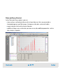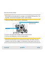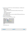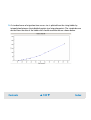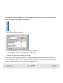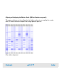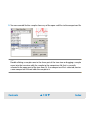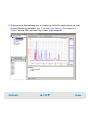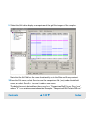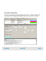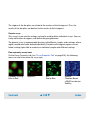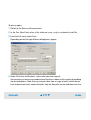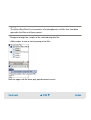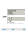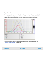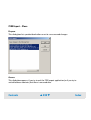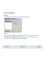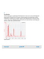
1
Agilent 2100 Bioanalyzer 2100 Expert User’s Guide Edition November 03 s1 Notices Warranty © Agilent Technologies, Inc. 2000-2003 No part of this manual may be reproduced in any form or by any means (including electronic storage and retrieval or translation into a foreign language) without prior agreement and written consent from Agilent Technologies, Inc. as governed by United States and international copyright laws. Manual Part number: G2946-90000 Edition: November 2003 Agilent Technologies, Deutschland GmbH Hewlett-Packard-Strasse 8 76337 Waldbronn The material contained in this document is provided “as is,” and is subject to being changed, without notice, in future editions. Further, to the maximum extent permitted by applicable law, Agilent disclaims all warranties, either express or implied, with regard to this manual and any information contained herein, including but not limited to the implied warranties of merchantability and fitness for a particular purpose. Agilent shall not be liable for errors or for incidental or consequential damages in connection with the furnishing, use, or performance of this document or of any information contained herein. Should Agilent and the user have a separate written agreement with warranty terms covering the material in this document that conflict with these terms, the warranty terms in the separate agreement shall control. Restricted Rights Legend Adobe and Acrobat are U.S. registered trademarks of Adobe Systems Incorporated. Microsoft® and Windows® are U.S. registered trademarks of Microsoft Corporation. Caliper®, LabChip and the LabChip logo are registered trademarks of Caliper Technologies Corp. in the U.S. and other countries. Technology Licenses The hardware and/or software described in this document are furnished under a license and may be used or copied only in accordance with the terms of such license. Contents If software is for use in the performance of a U.S. Government prime contract or subcontract, Software is delivered and licensed as “Commercial computer software” as defined in DFAR 252.227-7014 (June 1995), or as a “commercial item” as defined in FAR 2.101(a) or as “Restricted computer software” as defined in FAR 52.227-19 (June 1987) or any equivalent agency regulation or contract clause. Use, duplication or disclosure of Software is subject to Agilent Technologies’ standard commercial license terms, and non-DOD Departments and Agencies of the U.S. Government will receive no greater than Restricted Rights as defined in FAR 52.227-19(c)(1-2) (June 1987). U.S. Government users will receive no greater than Limited Rights as defined in FAR 52.227-14 (June 1987) or DFAR 252.227-7015 (b)(2) (November 1995), as applicable in any technical data. ▲2▼ Index Contents About this Manual .................................................................................................................. 6 In this Manual............................................................................................................................. 7 Related Documents ................................................................................................................... 9 What’s New in 2100 Expert.................................................................................................... 11 How to Use this Manual ......................................................................................................... 13 Quick Start ............................................................................................................................. 17 Looking at 2100 Expert ......................................................................................................... 31 Starting 2100 Expert ................................................................................................................ 32 2100 Expert Work Area ........................................................................................................... 33 Running a Demo Assay........................................................................................................... 41 Closing 2100 Expert ................................................................................................................. 45 Switching Between Electrophoretic and Flow Cytometric Assays ................................ 47 How to Prepare the Bioanalyzer for Electrophoretic Assays............................................ 49 How to Prepare the Bioanalyzer for Flow Cytometric Assays.......................................... 52 Running and Evaluating Electrophoretic Assays .............................................................. 55 Principles of Nucleic Acid and Protein Analysis on a Chip............................................... 56 Preparing and Running an Electrophoretic Assay.............................................................. 60 Analyzing and Evaluating the Results of an Electrophoretic Assay ................................ 91 ▲3▼ Index Result Flagging ....................................................................................................................... 145 Running and Evaluating Flow Cytometric Assays........................................................... 156 Principles of Flow Cytometric Measurements .................................................................. 157 Overview of Flow Cytometric Assays ................................................................................. 166 Preparing and Running a Flow Cytometric Assay ............................................................ 169 Analyzing and Evaluating the Results of a Flow Cytometric Assay............................... 198 Working with Chip and Assay Data.................................................................................. 245 2100 Expert Data Overview .................................................................................................. 246 Handling Assays..................................................................................................................... 249 Handling Chip Data ................................................................................................................ 253 Organizing, Retrieving, and Backing up 2100 Expert Data .............................................. 255 Importing Data........................................................................................................................ 256 Exporting Data ........................................................................................................................ 263 Printing Reports ..................................................................................................................... 275 Configuring Tables................................................................................................................. 282 Reading the Log Books ......................................................................................................... 287 Configuring 2100 Expert ..................................................................................................... 293 How to Specify Data File Names and Directories............................................................. 294 How to Set the Acoustic Chip Alert .................................................................................... 296 How to Specify Graph Settings............................................................................................ 298 Contents ▲4▼ Index How to Use the Advanced Settings .................................................................................... 299 Running Instrument Diagnostics ...................................................................................... 303 How to Run Instrument Diagnostics Tests........................................................................ 308 Performing Qualifications.................................................................................................. 312 2100 Expert Software Reference ....................................................................................... 320 2100 Expert Application Window Elements ...................................................................... 321 Dialog Boxes........................................................................................................................... 494 Shortcuts and Mouse Actions ............................................................................................. 565 Products, Spare Parts, and Accessories.......................................................................... 573 Glossary ............................................................................................................................... 576 Contents ▲5▼ Index About this Manual Welcome to the User’s Guide for the Agilent 2100 expert software. This manual provides beginners and advanced users with information needed to successfully run electrophoretic and flow cytometric assays with the bioanalyzer. The 2100 expert software allows the control of the bioanalyzer (including diagnostic functions) and, in combination with a LabChip kit, the acquisition, interpretation and result presentation of data generated during the analysis of DNA, RNA, proteins, and cells. Contents ▲6▼ Index In this Manual This manual provides bioanalyzer users with the following information: • “About this Manual” on page 6 gives an overview of the subjects in this manual, and lists major innovations and improvements of the 2100 expert software. It also lists supplemental literature and shows you how to make efficient use of this manual. • “Quick Start” on page 17 is meant for experienced users. It briefly summarizes the necessary steps to prepare and run an assay. • “Looking at 2100 Expert” on page 31 shows how to get started with the 2100 expert software, and outlines its main operational possibilities. • “Switching Between Electrophoretic and Flow Cytometric Assays” on page 47 shows you how to change cartridges, which is necessary for switching between electrophoretic and flow cytometric measurements. • “Running and Evaluating Electrophoretic Assays” on page 55 explains how electrophoretic measurements are made using the bioanalyzer, gives detailed descriptions of all steps necessary to run electrophoretic assays, and shows how to analyze and evaluate measurement results using electropherograms and gel-like images. • “Running and Evaluating Flow Cytometric Assays” on page 156 explains how flow cytometric measurements are made using the bioanalyzer, gives detailed descriptions of all steps necessary to run flow cytometric assays, and shows how to analyze and evaluate measurement results using histograms and dot plots. • “Working with Chip and Assay Data” on page 245 shows you what to do to open, save, import and export files, and how to print the measurement results. Contents ▲7▼ Index • “Configuring 2100 Expert” on page 293 is your guideline for configuring the 2100 expert software. • “Running Instrument Diagnostics” on page 303 shows how to use the diagnostics tests to check the bioanalyzer hardware for proper functioning. • “Performing Qualifications” on page 312 describes how you can validate your bioanalyzer system. • “2100 Expert Software Reference” on page 320 describes all elements of the 2100 expert user interface, such as screen regions, menus, tool bars, and dialog boxes. • “Products, Spare Parts, and Accessories” on page 573 lists all parts and accessories—including reorder numbers—that are required for electrophoretic and flow cytometric measurements. • “Glossary” on page 576 explains terms in context with flow cytometry, electrophoresis, and terms specific to the bioanalyzer software and hardware. If you have any questions this manual cannot answer, please refer to the supplemental literature listed in “Related Documents” on page 9. If you still have questions, contact Agilent for additional support at: http://www.agilent.com/chem/labonachip Contents ▲8▼ Index Related Documents A collection of supplemental literature is given in the following. Bioanalyzer Manuals Publication Number Title G2938-90006 Agilent 2100 Bioanalyzer Installation and Safety Manual G2946-90001 Agilent 2100 Bioanalyzer Maintenance and Troubleshooting Guide CD-ROM Publication Number Title G2946-60002 Agilent 2100 Bioanalyzer – How to Use Multimedia CD-ROM Reagent Kit Guides The Reagent Kit Guides give you information on how to prepare samples. Publication Number Title G2938-90300 Kit Guide Binder english (including all Reagent Kit Guides) G2938-90010 Reagent Kit Guide DNA 500 and DNA 1000 Assay G2938-90020 Reagent Kit Guide DNA 7500 and DNA 12000 Assay Contents ▲9▼ Index Publication Number Title G2938-90030 Reagent Kit Guide RNA 6000 Nano Assay G2938-90040 Reagent Kit Guide RNA 6000 Pico Assay G2938-90050 Reagent Kit Guide Protein 200 Plus Assay G2938-90060 Reagent Kit Guide Protein 50 Assay G2938-90070 Reagent Kit Guide Cell Fluorescence Assays G2938-90080 Reagent Kit Guide Cell Fluorescence Checkout Kit Application Notes and Technical Notes Application Notes and Technical Notes are available from the Agilent 2100 Bioanalyzer Help Desk or from the lab-on-a-chip web pages: http://www.agilent.com/chem/labonachip Newly Published Documentation Follow this link to see if there is any new documentation: http://www.chem.agilent.com/scripts/Library.asp Contents ▲ 10 ▼ Index What’s New in 2100 Expert Products 2100 expert is the successor to the Bio Sizing and Cell Fluorescence software. • 2100 expert provides a single software platform with a common user interface for running, analyzing, evaluating, presenting, and comparing DNA, RNA, protein and cell parameters. • 2100 expert is installed in one go. After installation, the functionality for electrophoretic and flow cytometric assays can be activated separately with license keys. Features 2100 expert integrates the complete Bio Sizing and Cell Fluorescence functionality plus additional features: • 2100 expert allows having multiple chip data and/or assay files open at the same time. • 2100 expert provides detailed installation qualification (IQ) and operational qualification (OQ) tests on both the bioanalyzer hardware and software. • 2100 expert features a new integrated data evaluation tool (Comparison context) allowing comparison of measurement results (of same assay class) from different chips directly. A separate data evaluation tool is no longer necessary. • 2100 expert features improved integration including manual integration. • 2100 expert allows color-coded result flagging. Flagging rules can be applied to measurement results. • 2100 expert now has customizable result tables and gel-like images. Contents ▲ 11 ▼ Index • 2100 expert has improved instrument control. Two bioanalyzers can be controlled at one time. It is possible to run measurements as well as diagnostics tests on two bioanalyzers at the same time. • 2100 expert has improved printing and reporting functions. • 2100 expert has extended instrument diagnostics functionality. Contents ▲ 12 ▼ Index How to Use this Manual This manual uses convenient online navigation features and follows certain typographic conventions. Online Navigation Use the interactive bookmarks in this frame to move to your desired topic. Use Acrobat Reader’s navigation bar to move around within a topic. Click here to go to the table of contents. Click here to go to the index. Here is the current page number. ▲ Displays the previous page. ▼ Displays the next page. Contents ▲ 13 ▼ Index After you have chosen a topic with the bookmarks, use the buttons in Acrobat Reader’s tool bar to move around within the topic. Displays the next page. Returns to the previous view. Click several times to undo more view changes. Displays the previous page. Displays the first page. Displays the last page. Contents ▲ 14 ▼ Returns to the next view. Click several times to redo more view changes. Index Layout Conventions The following typographic conventions are used in this manual: Highlight Meaning Italic On-screen element Example: ... the OK button. Emphasis Example: Right-click the ... Term Example: Dot plots show events as dots. Reference to another document Example: Refer to the Agilent 2100 Bioanalyzer Troubleshooting and Maintenance Guide. Blue Cross-reference or hyperlink Examples: “What’s New in 2100 Expert” on page 11 http://www.agilent.com/chem/labonachip Courier Code Example: .. the command line parameter -port 2 ... Courier bold User input Example: Enter 50 MB. Contents ▲ 15 ▼ Index Safety Notices, Notes and Tips Safety notices, notes and tips in this document have the following meaning: WA R N I N G A warning notice denotes a hazard. It calls attention to an operating procedure, practice, or the like that, if not correctly performed or adhered to, could result in personal injury or death. Do not proceed beyond a warning notice until the indicated conditions are fully understood and met. C A U T IO N A caution notice denotes a hazard. It calls attention to an operating procedure, practice, or the like that, if not correctly performed or adhered to, could result in damage to the product or loss of important data. Do not proceed beyond a caution notice until the indicated conditions are fully understood and met. NOTE A note contains important, helpful, or additional information. TIP A tip usually points out a timesaving feature. Contents ▲ 16 ▼ Index Quick Start The following step-by-step instructions summarize the basic steps needed to perform a measurement with the Agilent 2100 bioanalyzer. Preparing the Agilent 2100 Bioanalyzer 1 Ensure that the proper cartridge is installed in the bioanalyzer. You can identify the installed cartridge by the number engraved in its front. Engraved number Note that there are also electrode cartridges without an engraved number. = Electrode Cartridge for electrophoretic assays = Pressure Cartridge for flow cytometric assays 2 If you have to change the cartridge, follow the instructions in “Switching Between Electrophoretic and Flow Cytometric Assays” on page 47. Contents ▲ 17 ▼ Index Switching on the Agilent 2100 Bioanalyzer 1 Make sure the bioanalyzer is connected to line power and connected to the PC. 2 Turn on the line switch at the rear of the instrument. The status LED at the front of the bioanalyzer should light up. Lid Status LED The status LED shows you the current status of the instrument. Signal Meaning Green light Instrument is switched on and ready for measurement. Green blinking Measurement is running. Orange blinking Instrument is busy (running self diagnostic, for example). Red light Instrument is not ready for measurement. Switch the instrument off and on again. If the problem persists, call Agilent service. Contents ▲ 18 ▼ Index Running a Measurement 1 To start the 2100 expert software on the connected PC, go to your desktop and double-click the following icon: After startup of the software, you enter the Instrument context: Contents ▲ 19 ▼ Index In the upper left of the Instrument tab, an icon shows the status of the bioanalyzer: Icons Meaning Bioanalyzer detected, lid is open. Bioanalyzer detected. Lid is closed, but no chip is inserted. No bioanalyzer has been detected. Check the COM Port setting (see figure under step 3), the RS 232 connection cable, the power cable, and the power switch. For details on how to set up the bioanalyzer and connect it to a PC, see Agilent 2100 Bioanalyzer Installation and Safety Guide. 2 Make sure that a bioanalyzer has been detected before continuing. Contents ▲ 20 ▼ Index 3 Select an assay for the chip run. On the Instrument tab, click the Assay... button. – OR – Click the Assays menu. Both will open the Assays menu, allowing you to select an assay from the submenus. – OR – You can also select File > Open File to Run.... This opens a dialog box allowing you to load either an assay (.xsy) or a chip data file (.xad). Contents ▲ 21 ▼ Index 4 Prepare the samples and the chip. For detailed information on sample and chip preparation refer to the – Reagent Kit Guides that are available for each reagent kit. – Application Notes that are available for each assay. NOTE When preparing chip and samples, pay attention to the essential measurement practices described in “Essential Measurement Practices (Electrophoretic Assays)” on page 67 and “Essential Measurement Practices (Flow Cytometric Assays)” on page 178. 5 Insert the chip in the Agilent 2100 bioanalyzer: a Open the lid. The bioanalyzer icon changes as follows: b Check that the cartridge is inserted properly and the chip selector is in the correct position (“1” for electrophoretic assays, “2” for flow cytometric assays). For details, please refer to “Switching Between Electrophoretic and Flow Cytometric Assays” on page 47. Contents ▲ 22 ▼ Index c Place the chip into the receptacle. The figure shows this for an electrophoresis chip. Chip The chip fits only one way. Do not use force. C A U T IO N Do not force the lid closed. This may damage the cartridge. d Carefully close the lid. Electrophoretic assays: the electrodes in the cartridge fit into the wells of the chip. Flow cytometric assays: the adapter with the gasket in the cartridge fits onto the priming well of the chip. Contents ▲ 23 ▼ Index The bioanalyzer icon changes to a chip icon (a DNA chip icon, for example): If the chip is not detected, open and close the lid again. NOTE If the AutoRun option is active (see “Options – Advanced” on page 508), the chip run starts automatically once a chip has been inserted and the lid has been closed. 5 On the Instrument tab, click the Start button. Contents ▲ 24 ▼ Index The chip run starts. The Raw Signals sub-tab shows an electropherogram of the currently measured sample. The name of the sample is displayed above the graph. The graph is a “live” plot of the migration time against fluorescence units (raw data, including background fluorescence, for example). Contents ▲ 25 ▼ Index The number of the sample that is currently being measured is indicated on the information bar: The status bar shows the name of the currently measured sample, a progress bar showing the measurement progress for the current sample (not for the whole chip run), and the COM port number used for data acquisition: During the chip run, you can do the following: • View the chip data file in the Data and Assay context by clicking on the name of the Data File: • Switch to any other context. For example, you can evaluate any chip data file in the Data and Assay context, or compare samples in the Comparison context. • If necessary, abort the chip run by clicking on the Stop button. All data that was collected up to the stop point will be saved. Contents ▲ 26 ▼ Index Finishing the Measurement When the measurement is finished, the End of run dialog box appears, showing you the status of the assay and the file name where the chip run data has been stored. 1 To immediately view the results, select the Select file in Data Context check box, and click OK. Contents ▲ 27 ▼ Index This takes you to the Data and Assay context, and the data file that has just been generated by your chip run is selected. The Chip Summary tab shows information on your chip data file, and lets you enter comments regarding chip, samples, and study. Contents ▲ 28 ▼ Index 2 In the tree view panel, click any sample name, or the ladder. This selects the Electropherogram tab, which displays a data plot of migration time versus fluorescence intensity. Peaks have automatically been detected, and their characteristics such as size, concentration, and molarity have been calculated and are shown in the Peak Table at the bottom of the window. Contents ▲ 29 ▼ Index What You Can do When the Measurement is Finished When the measurement is finished, you can: • Document your chip run by entering sample names, chip comments, and study information, for example. • Evaluate the measurement results by analyzing gel-like images and electropherograms (electrophoretic assays), or histograms and dot plots (flow cytometric assays): – “Analyzing and Evaluating the Results of an Electrophoretic Assay” on page 91 – “Analyzing and Evaluating the Results of a Flow Cytometric Assay” on page 198 • Print the results to document them on paper. See “Printing Reports” on page 275. • Export the results for further evaluation in other applications. See “Exporting Data” on page 263. • Compare the results with the results of other chip runs in the Comparison context. • Insert the next chip in the bioanalyzer and start a new chip run with one click (provided that you will use the same assay). Contents ▲ 30 ▼ Index Looking at 2100 Expert Before you begin with running assays on the Agilent 2100 bioanalyzer you should familiarize yourself with the 2100 expert software: • “Starting 2100 Expert” on page 32 • “2100 Expert Work Area” on page 33 • “Running a Demo Assay” on page 41 • “Closing 2100 Expert” on page 45 Contents ▲ 31 ▼ Index Starting 2100 Expert To start 2100 expert: 1 Go to your desktop and double-click the following icon: – OR – From the Windows Start menu, select Programs > Agilent 2100 Bioanalyzer > 2100 expert. The 2100 expert application window appears. “2100 Expert Work Area” on page 33 gives an overview of the application window. Contents ▲ 32 ▼ Index 2100 Expert Work Area The 2100 expert work area has standard elements such as pull-down menus and toolbars, and the main working area, which contains several tabs, some of which have sub-tabs. The 2100 expert work area has the following regions (Data and Assay context): Title Bar Menu Bar Toolbars Info Bar Context Bar Tree View Tabs Sub-tabs Lower Panel Status Bar Setpoint Explorer See “2100 Expert Application Window Elements” on page 321 for details on the regions. Contents ▲ 33 ▼ Index The 2100 expert software can be operated in four modes, called “contexts”: • Instrument Context • Data and Assay Context • Validation Context • Comparison Context NOTE The contexts are independent from each other regarding their data. This means, for example, that you can review data and run measurements at the same time. Using the Contexts bar, the Context menu, or the drop-down list in the tool bar, you can switch between the contexts: Contents ▲ 34 ▼ Index NOTE Menus, toolbars, the tree view, and the main working area (tabs) significantly change when you switch between the contexts. An introduction to the four contexts is given in the following. Contents ▲ 35 ▼ Index Instrument Context On startup, 2100 expert enters the Instrument context, where you can run DNA, RNA, protein or cell assays by selecting an assay file and starting the chip run—provided that the bioanalyzer is properly connected, a chip is inserted, and the bioanalyzer lid is closed. Contents ▲ 36 ▼ Index NOTE If two bioanalyzers are connected to your PC, you can run both in parallel. During the chip run(s), you can view the status of the bioanalyzer(s): instrument information and real time acquisition data. In the Instrument context, it is also possible to run hardware diagnostic tests on all connected bioanalyzers. Refer to “Running Instrument Diagnostics” on page 303 for details. Contents ▲ 37 ▼ Index Data and Assay Context In the Data and Assay context, you can • view, analyze, and evaluate the results of your chip runs that are presented as electropherograms, gel-like images, histograms, dot plots, and result tables. • export and print the results of your chip runs. • modify existing assays and create your own assays by modifying properties such as data analysis setpoints. Contents ▲ 38 ▼ Index Validation Context The Validation context is used to run and document qualification tests. For both the bioanalyzer hardware and software tests can be run for: • Installation qualification (IQ) • Operational qualification (OQ) Validation results are automatically saved in .xvd files. You can re-open .xvd files to review validation results. For details, refer to “Performing Qualifications” on page 312. Contents ▲ 39 ▼ Index Comparison Context In the Comparison context, you can open multiple electrophoretic chip data files and compare samples of the same assay class (DNA 1000, for example), even from different chip runs. It is possible to overlay electropherograms recorded by the bioanalyzer, and compare the measurement results. Comparison results can be saved in .xac files. You can re-open .xac files to review the comparison results, and to add further samples for comparison, for example. Contents ▲ 40 ▼ Index Running a Demo Assay 2100 expert provides demo assays that you can use for a first impression of chip runs and data evaluation, even if the bioanalyzer is offline. To run a demo assay: 1 Start the software as described in “Starting 2100 Expert” on page 32, or, if the software is already running, switch to the Instrument context.s 2 On the Instrument tab, select “Demo” as the COM Port. 3 Click the Assay... button. Contents ▲ 41 ▼ Index This opens a menu, allowing you to select an assay from submenus. 4 Select a demo assay, for example Demo > electrophoresis > Demo Protein 200 Plus. The assay is loaded and a violet chip icon appears indicating the assay type “Protein”. 5 Click the Start button. Contents ▲ 42 ▼ Index The demo chip run starts and you can watch its progress on the Raw Signals tab, where you can see a simulation of data acquisition. For details on how a chip run proceeds, refer to “Running an Electrophoretic Assay” on page 72, or “Running a Flow Cytometric Assay” on page 182. NOTE Like a real chip run, a demo chip run also creates a chip data (.xad) file. Contents ▲ 43 ▼ Index At the end of the simulation, the End of run dialog box appears. 6 Select the Select file in Data Context check box and click OK. This takes you to the Data and Assay context where you can view the results and practice data analysis and evaluation as described in “Analyzing and Evaluating the Results of an Electrophoretic Assay” on page 91 and “Analyzing and Evaluating the Results of a Flow Cytometric Assay” on page 198. Contents ▲ 44 ▼ Index Closing 2100 Expert To close 2100 expert: 1 From the File menu, select Exit. 2100 expert quits. However, if a chip run is in progress, the following message appears: Click OK and wait until the chip run is complete. Contents ▲ 45 ▼ Index Also the following dialog box may appear: NOTE This dialog box may also appear if you try to switch between contexts but there is unsaved data. – Click Yes to save the changes to the selected files and continue quitting 2100 expert. If you want to save changes only to particular files, select these files in the list by single-clicking them. By default, all files with unsaved changes are selected. – If you click No, 2100 expert quits without saving any changes. – If you do not want to quit 2100 expert at this time, click Cancel to return to your 2100 expert session without saving anything. Contents ▲ 46 ▼ Index Switching Between Electrophoretic and Flow Cytometric Assays The Agilent 2100 bioanalyzer supports electrophoretic assays (DNA, RNA, and protein) and flow cytometric assays (apoptosis, for example). The bioanalyzer uses different cartridges for electrophoretic and flow cytometric assays: Electrode Cartridge for electrophoretic assays Contents Pressure Cartridge for flow cytometric assays ▲ 47 ▼ Index • The electrode cartridge contains 16 electrodes that fit into the wells of DNA, RNA, and Protein chips. Each electrode in the cartridge has an individual power supply. All electrophoretic assays (DNA, RNA, and Protein) require an electrode cartridge. The electrode cartridge can be identified by the engraved number “1” on the front. • The pressure cartridge contains a tubing and filter assembly that connect to the vacuum pump. The seal has to match the priming well on the chip so that the required low pressure can be built up. The pressure cartridge can be identified by the engraved number “2” on the front. NOTE There are also cartridges without an engraved number. These are all electrode cartridges. If the bioanalyzer is set up for flow cytometric assays, but you want to run electrophoretic assays, proceed as described in “How to Prepare the Bioanalyzer for Electrophoretic Assays” on page 49. If the bioanalyzer is set up for electrophoretic assays, but you want to run flow cytometric assays, proceed as described in “How to Prepare the Bioanalyzer for Flow Cytometric Assays” on page 52. Contents ▲ 48 ▼ Index How to Prepare the Bioanalyzer for Electrophoretic Assays Remove the pressure cartridge: 1 Turn off line power to the Agilent 2100 bioanalyzer. The line switch is located at the rear. 2 Open the lid. 3 Pull down the metal locking lever as shown in the figure below. Metal lever in open position The cartridge is pushed out. 4 Gently pull the cartridge out of the lid. NOTE Store the pressure cartridge in the provided box. Contents ▲ 49 ▼ Index Insert the electrode cartridge: C A U T IO N Do not touch the electrodes while the cartridge is in the Agilent 2100 bioanalyzer. The electrodes and the high voltage power supplies can be damaged. 1 Slide the electrode cartridge in the lid as shown below. Push here to ensure tight connection Metal lever 2 Push the metal front of the cartridge to ensure a tight connection. 3 Push the metal locking lever in the flat (closed) position. C A U T IO N Do not force the lid closed. This may damage the cartridge. If the lid does not close completely, check that the cartridge is inserted properly and try again to close the lid. Contents ▲ 50 ▼ Index 4 Remove any chip. C A U T IO N Do not force the chip selector handle when a chip is inserted in the bioanalyzer. 5 Adjust the chip selector to position “1” as shown in the following figure. To avoid using incompatible chips and cartridges, a chip selector is installed in the bioanalyzer. This ensures that the chip matches to the installed cartridge. Move chip selector in position “1” This will allow you to insert DNA, RNA, and Protein chips in the bioanalyzer. Contents ▲ 51 ▼ Index How to Prepare the Bioanalyzer for Flow Cytometric Assays Remove the electrode cartridge: 1 Turn off line power to the Agilent 2100 bioanalyzer. The line switch is located at the rear. 2 Open the lid. C A U T IO N Do not touch the electrodes while the cartridge is in the Agilent 2100 bioanalyzer. The electrodes and the high voltage power supplies can be damaged. 3 Pull down the metal locking lever in the open position as shown in the figure below. Metal lever in open position The cartridge is pushed out. 4 Gently pull the cartridge out of the lid. Contents ▲ 52 ▼ Index C A U T IO N Store the electrode cartridge in the provided box. If the pins of the electrode cartridge are bent or misaligned, poor quality results or pre-terminated chip runs will result. Insert the pressure cartridge: 1 Slide the pressure cartridge in the lid as shown below. Push here to ensure tight connection Metal lever 2 Push the metal front of the cartridge to ensure a tight connection. 3 Push the metal locking lever in the flat (closed) position. C A U T IO N Do not force the lid closed. This may damage the cartridge. If the lid does not close completely, check that the cartridge is inserted properly and try again to close the lid. Contents ▲ 53 ▼ Index 4 Remove any chip. C A U T IO N Do not force the chip selector handle when a chip is inserted in the bioanalyzer. 5 Adjust the chip selector to position “2” as shown in the following figure. To avoid using incompatible chips and cartridges, a chip selector is installed in the bioanalyzer. This ensures that the chip matches to the installed cartridge. Move chip selector in position “2” This will allow you to insert cell chips in the bioanalyzer. Contents ▲ 54 ▼ Index Running and Evaluating Electrophoretic Assays For running and evaluating electrophoretic assays you need to know the following: • “Principles of Nucleic Acid and Protein Analysis on a Chip” on page 56 • “Preparing and Running an Electrophoretic Assay” on page 60 • “Analyzing and Evaluating the Results of an Electrophoretic Assay” on page 91 • “Result Flagging” on page 145 Contents ▲ 55 ▼ Index Principles of Nucleic Acid and Protein Analysis on a Chip The electrophoretic assays are based on traditional gel electrophoresis principles that have been transferred to a chip format. The chip format dramatically reduces separation time and sample consumption. The system provides automated sizing and quantitation information in a digital format. On-chip gel electrophoresis is performed for the analysis of DNA, RNA and proteins. The chip accommodates sample wells, gel wells and a well for an external standard (ladder). Micro-channels are fabricated in glass to create interconnected networks among these wells. During chip preparation, the micro-channels are filled with a sieving polymer and fluorescence dye. Once the wells and channels are filled, the chip becomes an integrated electrical circuit. The 16-pin electrodes of the cartridge are arranged so that they fit into the wells of the chip. Each electrode is connected to an independent power supply that provides maximum control and flexibility. Charged biomolecules like DNA or Contents ▲ 56 ▼ Index RNA are electrophoretically driven by a voltage gradient—similar to slab gel electrophoresis. Because of a constant mass-to-charge ratio and the presence of a sieving polymer matrix, the molecules are separated by size. Smaller fragments are migrating faster than larger ones. Dye molecules intercalate into DNA or RNA strands or Protein-SDS micells. These complexes are detected by laser-induced fluorescence. Data is translated into gel-like images (bands) and electropherograms (peaks). With the help of a ladder that contains fragments of known sizes and concentrations, a standard curve of migration time versus fragments size is plotted. From the migration times measured for each fragment in the sample, the size is calculated. Two marker fragments (for RNA only one marker fragment) are run with each of the samples bracketing the overall sizing range. The “lower” and “upper” markers are internal standards used to align the ladder data with data from the sample wells. This is necessary to compensate for drift effects that may occur during the course of a chip run. For DNA and protein assays, quantitation is done with the help of the upper marker. The area under the upper marker peak is compared with the sample peak areas. Because the concentration of the upper marker is known, the concentration for each sample can be calculated. Besides this relative quantitation, an absolute quantitation is available for protein assays, using external standard proteins. For RNA assays, quantitation is done with the help of the ladder area. The area under the ladder is compared with the sum of the sample peak areas. The area under the “lower” marker is not taken into consideration. For total RNA assays, the ribosomal ratio is determined, giving an indication on the integrity of the RNA sample. Contents ▲ 57 ▼ Index The 2100 expert software plots fluorescence intensity versus migration time and produces an electropherogram for each sample: Contents ▲ 58 ▼ Index The data can also be displayed as a densitometry plot, creating a gel-like image: Contents ▲ 59 ▼ Index Preparing and Running an Electrophoretic Assay An electrophoretic chip run requires the following steps: 1. Set up and switch on the Agilent 2100 bioanalyzer. Refer to “Switching Between Electrophoretic and Flow Cytometric Assays” on page 47. 2. Start the 2100 expert software. Details are given in “Starting 2100 Expert” on page 32. 3. Select an electrophoretic assay. See “Selecting an Electrophoretic Assay for a Chip Run” on page 62. 4. Prepare chip and samples. Refer to “Preparing Samples and Chips for Electrophoretic Assays” on page 66 and to the appropriate Application Note and Reagent Kit Guide. 5. Load the chip into the bioanalyzer. For details refer to “Loading the Electrophoresis Chip into the Bioanalyzer” on page 70. 6. Start the chip run. This is described in “Running an Electrophoretic Assay” on page 72. When the chip run has finished, you can: • Have a first look at the results (see “Displaying the Measurement Results (Electrophoresis)” on page 82). • Document the chip run (see “Entering Chip, Sample, and Study Information” on page 80). Contents ▲ 60 ▼ Index • Analyze and evaluate the results: – “Analyzing and Evaluating the Results of an Electrophoretic Assay” on page 91 – “Result Flagging” on page 145 Contents ▲ 61 ▼ Index Selecting an Electrophoretic Assay for a Chip Run To select an assay: 1 Switch to the Instrument context. 2 In the Tree View Panel, select the bioanalyzer you want to use. In the upper left of the Instrument tab, an icon shows the status of the bioanalyzer. You should see one of the following icons (lid open/closed), indicating that the bioanalyzer is detected by the system: Contents ▲ 62 ▼ Index 3 If you do not see one of these icons, check that the bioanalyzer is switched on and properly connected: – Check the COM port setting. – Make sure the bioanalyzer is physically connected to the PC (over the serial interface). – Check the power connection. – Check the power switch. If you need additional help, please refer to the Agilent 2100 Bioanalyzer Maintenance and Troubleshooting Guide. 4 Select an assay for the chip run. On the Instrument tab, click the Assay... button. – OR – Click the Assays menu. Contents ▲ 63 ▼ Index Both will open the Assays menu, allowing you to select an assay from the submenus. – OR – Select File > Open File to Run.... This opens a dialog box, allowing you to load either an assay (.xsy) or a chip data file (.xad). The type of assay you have to select depends on the experiment and the Reagent Kit you use to prepare your samples. Details on these assays are described in the Application Notes available for each assay and in the Reagent Kit Guide. 5 Select the desired assay, DNA 1000, for example. The assay is loaded and its name appears on the Information Bar: Contents ▲ 64 ▼ Index NOTE After a chip run, the results can be evaluated using a different electrophoretic chip data file (.xad) of the same assay type (DNA 1000 in this example). Refer to “Importing Data Analysis Setpoints” on page 259. 6 Select a Destination for the chip data file (.xad) generated as the result of the chip run: 7 Under Data Acquisition Parameters, enter the number of samples you want to be measured. The total number of samples that can be measured varies with the type of assay selected. With DNA and RNA Nano assays, 12 samples may be run; with RNA Pico assays, 11 samples may be run; and with Protein assays, the maximum number of samples is 10. When preparing the chip (see “Preparing Samples and Chips for Electrophoretic Assays” on page 66), keep in mind that you have to follow the sequence of the sample wells. For example, if you want to measure 3 samples, you have to fill the wells 1, 2, and 3 of your chip. Contents ▲ 65 ▼ Index Preparing Samples and Chips for Electrophoretic Assays Before you can fill a chip, you have to prepare the samples. To find out how to prepare the samples, refer to the various Reagent Kit Guides available for each LabChip kit. Please refer to these documents for further information and analytical specifications. In general, preparing an electrophoretic assay involves the following steps: • Check that you have everything listed in the appropriate Reagent Kit Guide. Be aware that there can be small but important differences between the different assays even for the same type of molecules (for example, between DNA 1000 and DNA 7500 assays). • Make sure you are familiar with the essential measurement practices (see below). • Before running the first RNA assay: decontaminate the electrodes. • Prepare all the reagent mixtures (for example, the gel-dye mix). • Load the gel-dye mix using the priming station. • Load the DNA/RNA marker solution. • Load the chip with ladder, samples and buffer (depending on assay). Contents ▲ 66 ▼ Index Essential Measurement Practices (Electrophoretic Assays) General: WA R N I N G Wear hand and eye protection and follow good laboratory practices when preparing and handling reagents and samples. WA R N I N G No data is available addressing the mutagenicity or toxicity of the dye/DMSO reagent. Because the dye binds to nucleic acids, it should be treated as a potential mutagen and used with appropriate care. The DMSO mixtures should be handled with particular caution as DMSO is known to facilitate the entry of organic molecules into tissues. We strongly recommend using double gloves when handling DMSO mixtures. • Handle and store all reagents according to the instructions given in the Reagent Kit Guides. • Avoid sources of dust or other contaminants. Foreign matter in reagents and samples or in the wells of the chip will interfere with assay results. • Always insert the pipette tip to the bottom of the well when dispensing the liquid. Placing the pipette at the edge of the well may lead to poor results due to the formation of a bubble on the bottom of the well. Contents ▲ 67 ▼ Index • Protect dye and gel-dye mix from light. Remove light covers only when pipetting. Dye decomposes when exposed to light. • Use a new syringe and electrode cleaner with each new LabChip kit. • Do not touch the Agilent 2100 bioanalyzer during a chip run and never place it on a vibrating ground. • Keep all reagents and reagent mixes refrigerated at 4 °C when not in use. • Allow all reagents and samples to equilibrate to room temperature for 30 minutes before use. • Use loaded chips within 5 minutes. Reagents might evaporate, leading to poor results. RNA Assays: • Always wear gloves when handling RNA, and use RNase-free tips, microfuge tubes and water. • It is recommended to denature all RNA samples and RNA ladder by heat before use (70 °C, 2 minutes). • Always vortex the dye concentrate for 10 seconds before preparing the gel-dye mix. Contents ▲ 68 ▼ Index Protein Assays: • Store Protein sample buffer at -20 °C upon arrival. Keep the vial in use at 4 °C to avoid freeze-thaw cycles. • Allow the dye concentrate to equilibrate to room temperature for 20 minutes before use, to make sure the DMSO is completely thawed. Protect the dye from light during that time. Vortex before use. • Allow all other reagents to equilibrate to room temperature for 10 minutes before use. • Use 0.5 ml tubes to denature samples. Using larger tubes may lead to poor results, caused by evaporation. Contents ▲ 69 ▼ Index Loading the Electrophoresis Chip into the Bioanalyzer After preparing the chip, you can insert it into the Agilent 2100 bioanalyzer. To load the chip into the bioanalyzer: 1 Open the lid. NOTE Before inserting the chip, check that the electrode cartridge is installed and the chip selector is in position “1”. For details, refer to “Switching Between Electrophoretic and Flow Cytometric Assays” on page 47. 2 Place the prepared chip into the receptacle. The chip fits only one way. Do not use force. Chip Chip selector in position “1” Contents ▲ 70 ▼ Index 3 Carefully close the lid. C A U T IO N Do not force the lid closed. This may damage the cartridge. If the lid does not close completely, check that the cartridge and chip are inserted properly, and the chip selector is in the correct position. The icon on the Instrument tab changes to a DNA chip icon, if a DNA assay is selected: If the chip is not detected, open and close the lid again. NOTE If the AutoRun option is active (see “Options – Advanced” on page 508), the chip run starts automatically once a chip has been inserted and the lid has been closed. Contents ▲ 71 ▼ Index Running an Electrophoretic Assay Running an electrophoretic assay in 2100 expert just means pressing a button. NOTE You can stop a chip run at any time, for example, if errors occurred, or if you are not satisfied with the quality of the measurement results, which you can observe during the chip run. See “Stopping a Chip Run” on page 77. Starting the Chip Run When you have loaded the chip, you can start the chip run: 1 On the Instrument tab, click the Start button. The chip run starts. The Raw Signals sub-tab shows an electropherogram of the currently measured sample. The name of the sample is displayed above the graph. The graph is a “live” plot of the migration time against fluorescence units (raw data, including background fluorescence, for example). Contents ▲ 72 ▼ Index The number of the sample that is currently being measured is indicated on the information bar: Contents ▲ 73 ▼ Index The status bar shows the name of the currently measured sample, a progress bar showing the measurement progress for the current sample (not for the whole chip run), and the COM port number used for data acquisition: During the chip run, you can do the following: • View the chip data file in the Data and Assay context by clicking on the name of the Data File: • Switch to any other context. For example, you can evaluate any chip data file in the Data and Assay context, or compare samples in the Comparison context. • If necessary, abort the chip run by clicking on the Stop button. All data that was collected up to the stop point will be saved. Contents ▲ 74 ▼ Index Finishing the Chip Run When the measurements are finished, the End of run dialog box appears, showing you the number of samples that have been measured, and the file name where the chip run data has been stored. If errors occurred, they would also be displayed in this dialog box. 1 To immediately view the results in the Data and Assay context, you can select the Select file in Data Context check box. 2 Click OK. Contents ▲ 75 ▼ Index The dialog box is closed. • If you selected Select file in Data Context, you are automatically taken to the Data and Assay context, where you can view, analyze, and evaluate the results of your chip run (see “Displaying the Measurement Results (Electrophoresis)” on page 82 and “Analyzing and Evaluating the Results of an Electrophoretic Assay” on page 91). • If you did not select the Select file in Data Context check box, you are taken back to the Instrument context, where you can start a new assay, for example. Contents ▲ 76 ▼ Index Stopping a Chip Run You can stop a chip run at any time, for example, • if the quality of the measurement results does not meet your expectations, • if, for example, after three samples you already have the information you desired and you want to start another chip run. NOTE You cannot resume a stopped chip run. NOTE If you stop a chip run, automatic export (see “Exporting Chip Run Data Automatically” on page 266) and automatic print (see “How to Turn on and Configure Automatic Printing of Chip Run Reports” on page 280) do not take place. To stop the assay: 1 Click the Stop button . – OR – Select Stop from the Instrument menu. NOTE Data acquisition of the current sample will be aborted. Contents ▲ 77 ▼ Index The following message appears: 2 Click Yes to stop the chip run. The End of Run dialog box appears. Contents ▲ 78 ▼ Index The measured samples are marked with a green check, and only these are stored in the chip data file. The unmeasured samples are marked with a white cross on red ground. 3 If you want to immediately view the results in the Data and Assay context, select the Select file in Data Context check box. 4 Click OK. The dialog box is closed. • If you selected Select file in Data Context, you are automatically taken to the Data and Assay context, where you can view, analyze, and evaluate the results (if any) of your chip run (see “Displaying the Measurement Results (Electrophoresis)” on page 82 and “Analyzing and Evaluating the Results of an Electrophoretic Assay” on page 91). • If you did not select the Select file in Data Context check box, you are taken back to the Instrument context, where you can start the next chip run, for example. Contents ▲ 79 ▼ Index Entering Chip, Sample, and Study Information During or after a chip run, you can document the run by entering information on chip, samples, and study. 1 In the Data and Assay context, select the Chip Summary tab. 2 On the Sample Information sub-tab, you can enter additional information such as sample names and comments. On the Study Information sub-tab, you can enter the laboratory location, and the name of the experimenter, for example. Contents ▲ 80 ▼ Index NOTE You may find some input fields already filled in, because chip, sample, and study information are taken over from the base assay or chip data file. For details on all input fields, refer to “Chip Summary Tab” on page 427. 3 Click Apply. 4 From the File menu, select Save. TIP You can import chip, sample, and study information from .txt or .csv files. This is especially helpful and time-saving, if you already have documented a similar chip run in another chip data file. Refer to “Importing Chip, Sample, and Study Information” on page 261 for details. Contents ▲ 81 ▼ Index Displaying the Measurement Results (Electrophoresis) You can view the measurement results of an electrophoretic chip run as electropherograms or gel-like images. • You can display the electropherograms either one sample at a time, or all samples at the same time to get an overview of the chip run, for example, to see the progress of a reaction. See “How to Switch Between Single View and Grid View (Electropherograms)” on page 83. • You can navigate through the samples. See “How to Navigate Through the Samples” on page 84. • You can change the display of electropherograms and gel-like images to make details better visible. See “How to Change the Display of Electropherograms and Gel-like Images” on page 85. Contents ▲ 82 ▼ Index How to Switch Between Single View and Grid View (Electropherograms) To switch between single view and grid view: 1 From the Electropherogram menu, select View Single Sample or View All Samples. – OR – Click the View Single Sample Electropherogram tool bar. or View All Samples button on the – OR – Click the All Samples entry in the Tree View Panel to switch to the grid view, or any sample name to switch to the single view. – OR – Double-click any electropherogram the grid view to switch to single view: Contents ▲ 83 ▼ Index How to Navigate Through the Samples At any time—even during a chip run—you can scroll through all samples—either in electropherogram or gel view. To navigate through samples using the Tree View Panel: 1 If the tree view is not visible, select View > Tree View. The tree view panel appears to the left of the tabs, and shows all chip data and assay files as nodes. 2 Click any sample name. Electropherogram view: the electropherogram of the selected sample is shown in single view Gel view: the lane of the gel-like image corresponding to the selected sample is highlighted. To navigate through samples using the Lower Panel: 1 If the lower panel is not visible, select View > Lower panel. The lower panel appears in the lower left corner. 2 Electropherogram view: Click on any lane of the small gel image. Gel view: Click on any well on the chip icon. Contents ▲ 84 ▼ Index To browse through samples: 1 From the Electropherogram or Gel menu, select Next Sample or Previous Sample. – OR – Click the Next Sample or Previous Sample button in the tool bar. To switch between electropherogram and gel view: 1 Click the Electropherogram or Gel tab to display the results of the selected sample as an electropherogram or as a gel-like image. How to Change the Display of Electropherograms and Gel-like Images It is possible to change the display of electropherograms and gel-like images. In electropherograms and gel-like images you can: • zoom (enlarge or reduce using the mouse) the graphs to display details, for example. In electropherograms, you can additionally: • show data points. • pan and scale the graph using the mouse. • change the background from white to a gray-to-white gradient. • remove the grid from the electropherograms. In gel-like images, you can additionally: • change the gel color. Contents ▲ 85 ▼ Index To zoom into an electropherogram: 1 From the Electropherogram menu, select Graph Mode > Zoom (default setting). 2 Position the mouse pointer in the electropherogram. 3 Click and hold down the left mouse button. The mouse pointer changes its shape to a magnifying glass . 4 Drag the mouse. A rectangle shows the part of the an electropherogram to be enlarged. 5 Release the mouse button. Contents ▲ 86 ▼ Index To pan and scale an electropherogram: 1 From the Electropherogram menu, select Graph Mode > Pan or Scale. 2 Position the mouse pointer in the electropherogram. 3 Click and hold down the left mouse button. The mouse pointer changes its shape to a double-arrow or to a double crosshair. 4 Drag the mouse. As you drag the mouse, the electropherogram curve moves in the drag direction (Pan mode), or the scales of the X and/or Y axes change (Scale mode). 5 Release the mouse button. You can perform several zoom, pan and scale steps in a row. To undo one zoom, pan, or scale step: 1 Click the Undo Zoom button or double-click in the electropherogram. To undo all zoom, pan, and scale steps: 1 Click the Undo All Contents button. ▲ 87 ▼ Index To display data points in an electropherogram: 1 From the Electropherogram menu, select Show Data Points or click the toolbar. button in the Data points used to generate the graph are now shown as bullets. Data points are 0.05 seconds apart. To put a color gradient on the background of an electropherogram: 1 From the Electropherogram menu, select Show Gradient. A color gradient (gray to white) appears on the background of the graph. To show/hide the grid lines on an electropherogram: 1 From the Electropherogram menu, select Show Grid. Contents ▲ 88 ▼ Index Cleaning the Electrodes after an Electrophoretic Assay When the assay is complete, remove the used chip from the bioanalyzer and dispose of it according to the guidelines established by your laboratory safety officer. Remove the chip quickly to prevent a buildup of residues from the solutions on the electrodes. Then perform the cleaning procedure to ensure that the electrodes are clean (i.e., no residues left from the previous assay). The cleaning procedures are described in detail in the appropriate Reagent Kit Guide and in the Agilent 2100 Bioanalyzer Maintenance and Troubleshooting Guide. Good Practices • Empty and refill the electrode cleaner at regular intervals (e.g., every five assays). • The electrode cleaner can be used for 25 assays. Contents ▲ 89 ▼ Index C A U T IO N Never use a cloth to clean the electrodes. Electrostatic discharge could damage the high-voltage power supplies. C A U T IO N Wet electrodes can cause severe damage to the on-board high voltage power supplies. Always make sure the electrodes are dry before inserting them into the bioanalyzer again. Contents ▲ 90 ▼ Index Analyzing and Evaluating the Results of an Electrophoretic Assay The purpose of electrophoretic assays is to calculate the size and concentration of nucleic acid fragments. Results for a particular sample are calculated after all data for that sample has been read. The steps in data analysis differ depending on the type of assay in use: • “Data Analysis: DNA” on page 92 • “Data Analysis: RNA and Cy5-Labeled Nucleic Acids” on page 97 • “Data Analysis: Protein” on page 100 • “Smear Analysis” on page 105 Further steps in analysis are: • “Changing the Data Analysis” on page 111 • “Reanalyzing a Chip Data File” on page 134 • “Comparing Samples from Different Electrophoretic Chip Runs” on page 136 Contents ▲ 91 ▼ Index Data Analysis: DNA The data analysis process for DNA assays consists of the following steps: 1. Raw data is read and stored by the system for all of the individual samples. 2. The data is filtered and the resulting electropherograms of all samples are plotted. You can change the settings of the data analysis after the run and reanalyze your data. 3. Peaks are identified for all samples and are tabulated by peak ID. You can change the settings of the peak find algorithm and reanalyze the data after the run has finished. (Note that peak find settings can be changed for all or only certain samples.) Contents ▲ 92 ▼ Index 4. A sizing ladder (see the example electropherogram below), which is a mixture of DNA fragments of known sizes, is run first from the ladder well. The concentrations and sizes of the individual base pairs are preset in the assay and cannot be changed. Contents ▲ 93 ▼ Index 5. A standard curve of migration time versus DNA size is plotted from the DNA sizing ladder by interpolation between the individual DNA fragment size/migration points. The standard curve derived from the data of the ladder well should resemble the one shown below. Contents ▲ 94 ▼ Index 6. Two DNA fragments are run with each of the samples, bracketing the DNA sizing range. The “lower marker” and “upper marker” are internal standards used to align the ladder data with data from the sample wells. The figure below shows an example of assigned marker peaks in a sample well. Lower marker Upper marker NOTE The software performs alignment by default. Turning automatic data analysis off (see “Electropherogram Menu” on page 345) suspends data analysis until you turn it on again. 7. The standard curve, in conjunction with the markers, is used to calculate DNA fragment sizes for each sample from the migration times measured. Contents ▲ 95 ▼ Index 8. To calculate the concentration of the individual DNA fragments in all sample wells, the upper marker, in conjunction with an assay-specific concentration against base-pair size calibration curve, is applied to the individual sample peaks in all sample wells. NOTE The software allows you to redefine the peaks chosen as upper and lower markers. A change in marker selection will cause quantitative changes in the calibration procedure, however, and therefore in the entire data evaluation. 9. If the checkbox Rest. Digest on the Chip Summary Tab is enabled, the 2100 expert software flags peaks that may have co-migrated: Since it is assumed that the molarity of all the fragments in a restriction digest should be the same, any peaks or clusters having a molarity that is significantly larger than the rest are flagged as potentially co-migrating peaks, allowing you to examine them in more detail. Contents ▲ 96 ▼ Index Data Analysis: RNA and Cy5-Labeled Nucleic Acids The data analysis process for RNA and the Cy5-labeled nucleic acids assays consists of the following steps: 1. Raw data is read and stored by the system for all of the individual samples. 2. The data is filtered and the resulting electropherograms of all samples are plotted. You can change the settings of the data analysis after the run and reanalyze your data. 3. Fragments are identified for all samples and tabulated by peak ID. You can change the settings of the peak find algorithm for any or all samples and reanalyze the data. 4. An RNA ladder (containing a mixture of RNA of known concentration) is run first (see the electropherogram below). The concentrations and sizes of the individual base pairs are preset in the assay and cannot be changed. Electropherogram of RNA 6000 Ladder (Ambion, Inc. cat. no. 7152) Contents ▲ 97 ▼ Index NOTE Peak ratios for the RNA ladder may vary from one batch of RNA 6000 ladder to the next. Assay performance will not be affected by this variation. 5. For the Eukaryote or Prokaryote Total RNA assay, the RNA fragments (either 18S and 28S for eukaryotic RNA or 16S and 23S for prokaryotic RNA) are detected. After detection, the ratio of the fragment areas is calculated and displayed. 6. To calculate the concentration of the RNA, the area under the entire RNA electropherogram is determined. The ladder, which provides the concentration/area ratio, is applied to transform the area values into concentration values. Contents ▲ 98 ▼ Index RNA Assays The marker solution that is part of each RNA LabChip kit, contains a 50 bp DNA fragment. This fragment is used as lower marker to align all samples. By default the RNA alignment and the subtraction of the lower marker are enabled for RNA Nano assays. The marker is displayed as the first peak in the electropherogram: Lower marker Contents ▲ 99 ▼ Index Data Analysis: Protein The data analysis process for protein assays consists of the following steps: 1. Raw data is read and stored by the system for all of the individual samples. 2. The data is filtered and the resulting electropherograms of all samples are plotted. You can change the settings of the data analysis after the run and reanalyze your data. 3. Peaks are identified for all samples and are tabulated by peak ID. You can change the settings of the peak find algorithm and reanalyze the data after the run has finished. (Note that peak find settings can be changed for all or only certain samples.) Contents ▲ 100 ▼ Index 4. A sizing ladder (see the example electropherogram below), which is a mixture of proteins of different known sizes, is run first from the ladder well. The concentrations and sizes of the individual proteins are preset as kDa in the assay and cannot be changed. Contents ▲ 101 ▼ Index 5. A standard curve of migration time versus size is plotted from the sizing ladder by interpolation between the individual protein size/migration points. The standard curve derived from the data of the ladder well should resemble the one shown below. Contents ▲ 102 ▼ Index 6. Two proteins are run with each of the samples, bracketing the sizing range. The “lower marker” and “upper marker” proteins are internal standards used to align the ladder data with data from the sample wells. The figure below shows an example of assigned marker peaks in a sample well. Lower marker Upper marker NOTE The software performs alignment by default. Turning automatic data analysis off (see “Electropherogram Menu” on page 345) suspends analysis until you turn it on again. Contents ▲ 103 ▼ Index 7. The standard curve, in conjunction with the markers, is used to calculate protein sizes for each sample from the migration times measured. 8. To calculate the concentration of the individual proteins in all sample wells, the upper marker, in conjunction with an assay-specific concentration calibration curve, is applied to the individual sample peaks in all sample wells. NOTE The software allows you to define upper and lower markers yourself. A change in the selection of the markers will lead to quantitative changes in the calibration procedure, however, and therefore in the entire data evaluation. Contents ▲ 104 ▼ Index Smear Analysis The 2100 expert software allows to perform a smear analysis for all electrophoresis assays. When the smear analysis is enabled, the software allows you to define regions of interest. These regions are used to define the area of broad peaks and determine their part of the total area. Smear analysis provide a means to analyze broad signals that can be hardly evaluated with the normal peak assignment. You therefore can define regions of interest that contain the peaks (base pair size) that you are interested in. For these regions you can determine the covered area in relation to the total area. Enabling Smear Analysis To enable smear analysis: 1 Go to the Electropherogram tab in the Data and Assay context: 2 Go to the setpoint explorer and select the Local or Global tab, depending on which samples should be analyzed. 3 Select the Advanced mode. Contents ▲ 105 ▼ Index 4 Under Smear Analysis select the checkbox Perform Smear Analysis. 5 Click the Apply button that changes become effective. Contents ▲ 106 ▼ Index Performing Smear Analysis After enabling the smear analysis in the setpoint explorer, you are able to insert regions of interest in the electropherogram. To do so: 1 Select the Region Table sub-tab in the Electropherogram tab. 2 Right-click the electropherogram and select Add region. A region will be inserted into the electropherogram. The Region Table will show values for the inserted region. Contents ▲ 107 ▼ Index 3 Repeat the previous step until the number of required regions are inserted. 4 Adjust the regions by directly moving the dashed lines in the electropherogram. 5 To remove a region, right-click the dashed line in the electropherogram and select Remove Region from the context menu. Contents ▲ 108 ▼ Index NOTE The smear analysis table can be directly edited by selecting the region table under Smear Analysis in the setpoint explorer. Contents ▲ 109 ▼ Index In the smear analysis table, you can edit the Region Start Size and Region End Size, for example: Contents ▲ 110 ▼ Index Changing the Data Analysis Different sets of parameters (data analysis setpoints) can be changed in the software in order to modify the data evaluation for sample analysis. For all assays: • Filtering parameters • Peak find parameters for all samples/peak height for individual samples • Enabling smear analysis • Align to upper and/or lower marker For RNA assays only: • Adding/deleting ribosomal fragments These settings can be made before a new run is started or when reanalyzing a previously saved data file. Contents ▲ 111 ▼ Index About the Setpoint Explorer The tool allowing you to modify the data analysis setpoints is the Setpoint Explorer. The setpoint explorer is accessible from: • Assay Properties Tab • Electropherogram Tab (Single/Grid View) • Gel Tab On the Assay Properties tab, the setpoint explorer is always visible and lets you modify setpoints globally (for all samples): Contents ▲ 112 ▼ Index To show the setpoint explorer, on the Electropherogram/Gel tab, click the vertical bar on the right edge of the application window: The setpoint explorer appears. For electrophoretic assays, you can modify the setpoints • either globally, that is, for all samples (Global tab), • locally, for the current sample (Local tab). Click the + nodes to expand, and the – nodes to collapse branches. Setpoints that you can change are white. To edit a setpoint, double-click the value, enter the new value, and press enter. Edited values are red (until you apply them): Contents ▲ 113 ▼ Index Changing any global setpoints while local settings have been applied opens a dialog box asking whether to override custom sample settings: Choosing Yes causes any changes made to the setpoints for individual samples to be discarded and applies the changes globally to all samples. Choosing No causes individual samples to retain changed setpoints. Contents ▲ 114 ▼ Index Filtering Setpoints The first step the software takes in analyzing the raw data is to apply data filtering. The following filtering setpoints can be changed: Filter Width Defines the data window, given in seconds, used for averaging. The broader the filter width, the more raw data points are used for averaging. As a result, the noise level will decrease, but peaks will become lower and broader. Overall, changing the Filter Width has more effect on the result of the filtering procedure applied then does changing the Polynomial Order. Polynomial Order This setting is used to define the power series applied to fit the raw data. The higher the number, the more the fit function will follow the noisy raw data curve. As a result, the noise level of the filtered curve will increase. Peak Find Setpoints After data filtering, the peak find algorithm locates the peaks and calculates the local peak baselines. The algorithm begins by finding all the peaks above the noise threshold in order to determine the baseline, after which any peaks below the noise threshold are rejected. A local baseline is calculated for each peak to allow for baseline drift. Contents ▲ 115 ▼ Index The four peak find setpoints that can be changed are: Min Peak Height The Min Peak Height setpoint determines whether a peak is kept. For each peak, the difference between the start point value and the center point value (local baseline) must be greater than the Min Peak Height value. Min Peak Width The Min Peak Width setpoint determines the minimum amount of time that must elapse before a peak is recognized. Slope Threshold The Slope Threshold setpoint determined the difference in the slope that must occur in order for a peak to begin. The inverse of this value is used to determine the peak end. Baseline Plateau The Baseline Plateau setpoint is a parameter that assists in finding peaks. The signal is recognized to be at baseline whenever the slope of the data is less than the Slope Threshold setpoint (either positive or negative) for longer than the time set for the Baseline Plateau. This setting rejects brief, low slope areas such as between non-baseline-resolved peaks. Contents ▲ 116 ▼ Index Manually Moving Fragment Start and End Points (RNA and Cy5-Labeled Nucleic Acids) It is also possible to alter the start and end points manually for individual fragments in an RNA or Cy5-labeled nucleic acids assay. Zooming in on the base of a particular fragment allows you to see the start and end points. Placing the cursor over one of these points changes the cursor to a pointing hand, allowing you to click and drag the point along the line of the fragment until it is positioned as desired. Move any other start or end points as desired. Contents ▲ 117 ▼ Index TIP The fragment table can be directly edited in the setpoint explorer: NOTE Changing the start or end points of the fragment will change the calculated rRNA ratio. It might be convenient to pause the automatic analysis (Electropherogram > Pause Automatic Analysis) until all changes are done. Contents ▲ 118 ▼ Index Setting the Baseline for Calculation of RNA Concentration At low signal-to-noise ratios, the baseline that defines the area used for calculating the concentration of RNA assays is highly dependent on the settings for the Start and End Time. You can adjust the Start and End Times manually (thereby adjusting the baseline) to ensure a good result even at very low signal-to-noise ratios. Choose a single sample. Two vertical green long-dashed lines indicating the setpoints for the Start and End Times (with the baseline drawn between them) are displayed in the window. Move the cursor over the long-dashed line on the left (Start Time setting) and drag the line to the desired position. Do the same with the long-dashed line on the right (End Time setting) until you have a flat baseline. NOTE Changing the start and end times will change the calculated RNA concentration. It might be convenient to pause the automatic analysis (Electropherogram > Pause Automatic Analysis) until all changes are done. Contents ▲ 119 ▼ Index Assigning Upper and Lower Marker Peaks For each DNA or protein sample, the upper and lower marker peaks are assigned first and then the data is aligned so that the sample markers match the ladder markers in time, allowing the size and concentration of the sample peaks to be determined. The first peak is assigned to be the lower marker and is then offset to match the lower marker in the ladder. The upper marker is then assigned to the last peak in the sample well or to the peak nearest the ladder’s upper marker. See an example of assigned marker peaks below. If you get unexpected peaks in the ladder analysis or find that the markers have been set incorrectly, you may exclude peaks manually from the ladder or set a peak to be used as a marker. Right-clicking in the peak table causes a context menu to appear, allowing you to do so: C A U T IO N Excluding a peak or manually setting a peak to be an upper or lower marker for a DNA or protein assay can cause errors with analysis. Contents ▲ 120 ▼ Index Aligning or Unaligning the Marker Peaks (DNA or Protein assays only) The upper and lower are then aligned to the ladder markers by resampling the sample data in a linear stretch or compression using a point-to-point fit: Data before alignment Contents ▲ 121 ▼ Index Markers aligned to the ladder If the sample marker peaks are either more than twice as far apart or less than half as far apart as the ladder markers, they are assumed to be the wrong peaks, and analysis of the sample stops, producing the error “Marker peaks not detected”. Contents ▲ 122 ▼ Index NOTE With DNA and protein assays, the height of marker peaks is assay dependent. Ladder peaks are analyzed to calculate a marker peak threshold that is used to locate the marker peaks in the sample wells. If the marker peaks found using this calculated method fail to align with those of a sample, the 2100 expert software will use the minimum peak height threshold setting instead (if this value is lower than the value for the marker peak). For example, the calculated threshold might be too high to find the sample's markers if they happen to be very small for some reason. Either no markers will be found or the wrong peaks will be assumed to be markers and these may not align with the ladder markers. Consequently, the software attempts to use the minimum peak height threshold that, if it is set low enough, will catch the real markers, allowing the sample to align. NOTE After alignment, peaks are shown with relative migration times that are different from the real times with data unaligned. Contents ▲ 123 ▼ Index Manual Integration For all electrophoretic assays, the 2100 expert software allows to manually integrate peaks. Manual integration allows you to move, add or delete peak baselines. TIP To move a peak baseline, point along the vertical line, press the CTRL key and left mouse button. To move a peak baseline, point along the signal, press the left mouse button only. Example: Adjusting peak baselines To manually change peak baselines: 1 Highlight the Electropherogram tab in the Data and Assay context and zoom into the electropherogram to enlarge the peak of interest. 2 Select Electropherogram > Manual Integration to switch off the automatic integration. As an alternative you can click the Manual Integration button Contents ▲ 124 ▼ in the toolbar. Index The baseline points become visible as blue or green dots. Highlighted baseline points are labelled green and can be moved either along the vertical line (press CTRL key and left mouse button) or along the signal trace (left mouse button). The blue baseline points are fixed and cannot be moved. To highlight a baseline point, click on it. 3 Pause the automatic analysis by clicking the appropriate icon in the toolbar. TIP Before manual integration is done, it is strongly recommended to pause the automatic analysis and to restart it again when all changes are done. Otherwise data analysis starts every time, when the baseline points are moved. Contents ▲ 125 ▼ Index 4 Adjust the baseline points as appropriate. TIP To move a peak baseline point along the vertical line, press the CTRL key and the left mouse button. To move a peak baseline point along the signal, press the left mouse button only. 5 Click the Automatic Analysis button to enable the integration again. The integration results in the result and peak tables will change according to the changes done. Contents ▲ 126 ▼ Index Example: Removing peaks To remove peaks: 1 Highlight the Electropherogram tab in the Data and Assay context and zoom into the electropherogram to enlarge the peak of interest. 2 Select Electropherogram > Manual Integration to switch off the automatic integration. As an alternative you might click the Manual Integration button in the toolbar. The baseline points become visible as blue or green dots. Contents ▲ 127 ▼ Index 3 Right-click on a baseline-point and select Remove Peak from the context menu. The two baseline points and the connecting line will disappear and the integration results shown in the result and peak tables will be updated: Contents ▲ 128 ▼ Index Example: Inserting peak baselines To insert peaks manually: 1 Highlight the Electropherogram tab in the Data and Assay context and zoom into the electropherogram to enlarge the peak of interest. Contents ▲ 129 ▼ Index 2 Right-click on the electropherogram and select Add Peak from the context menu. Contents ▲ 130 ▼ Index 3 Two baseline points and the connecting line will appear and the integration results shown in the result and peak tables will be updated. 4 Pause the automatic analysis by clicking the appropriate icon Contents ▲ 131 ▼ in the toolbar. Index TIP Before manual integration is done, it is strongly recommended to pause the automatic analysis and to restart it again when all changes are done. Otherwise data analysis starts every time, when the baseline points are moved. 5 Adjust the baseline points as appropriate. TIP To move a peak baseline point along the vertical line, press the CTRL key and the left mouse button. To move a peak baseline point along the signal, press the left mouse button only. Contents ▲ 132 ▼ Index 6 Click the Automatic Analysis button to enable the integration again. The integration results in the result and peak tables will change according to the changes done. Contents ▲ 133 ▼ Index Reanalyzing a Chip Data File NOTE Occasionally you may wish to open and view or reanalyze a chip data file that was run and saved previously. The raw data values are saved in the data file, along with the analysis settings that were chosen for the run, so that the data can be reanalyzed with different settings. To do this: 1 Click File > Open... to open a chip data file (.xad). 2. Choose the filename from the list of data files. 3. Click OK. The items that can be changed for reanalysis are: All Assays: • Global peak find settings • Individual sample peak find settings • Expected base pair size for certain assays • Gel color • Sample names and comments • Manual integration Contents ▲ 134 ▼ Index RNA Assays Only: • Fragment names and colors associated with labels • Fragment start/end times, additional fragments (or delete fragments found) DNA and Protein Assays Only: • Exclude peaks from analysis • Reassign upper/lower markers • Alignment or no alignment with ladder peaks • Assay (you can save the changed settings under a new assay name, if desired) TIP When applying modified data analysis setpoints, the software will (by default) immediately recalculate the raw data, which takes some time. Select Don’t Analyze from the Gel Menu or Electropherogram Menu to temporarily switch off automatic data analysis while you modify setpoints. If you save the data file after making changes, it will keep a record of the changes such as gel color, sample names, and peak find settings that were in effect at the time the file is resaved. If you do not want to change the original file, choose File > Save As… and give the file a new name or save it to a different location. Contents ▲ 135 ▼ Index Comparing Samples from Different Electrophoretic Chip Runs The 2100 expert software allows you to compare the measurement results of samples from different electrophoretic chip runs. Samples to be compared must be from chip runs of the same assay type. In the Comparison context, you can create comparison files, include samples from different chip runs, and compare the samples by overlaying electropherograms, for example. To compare samples from different electrophoretic chip runs: 1 Switch to the Comparison context: 2 From the File menu select Open..., and open all chip data files (.xad) that contain the samples you want to compare. Contents ▲ 136 ▼ Index The .xad files appear in the Select Data Files list of the Tree View Panel. NOTE The Select Data Files list also contains all electrophoretic .xad files that are open in the Data and Assay context. 3 Select a .xad file from the Select Data Files list to display a list of its samples. 4 Right-click a sample name and select Add Sample to New Comparison File. Contents ▲ 137 ▼ Index A new comparison file appears in the upper part of the tree view containing the sample. The sample is selected and its electropherogram is shown. Note that the Electropherogram Tab (Single/Grid View) a has the same functionality as in the Data and Assay context. Contents ▲ 138 ▼ Index 5 You can now add further samples from any of the open .xad files to the comparison file. TIP Double-clicking a sample name in the lower part of the tree view or dragging a sample name into the tree view adds the sample to the comparison file that is currently selected in the upper part of the tree view. Or, if no comparison file is selected, creates a new comparison file and adds the sample to it. Contents ▲ 139 ▼ Index The following message appears if you try to add a sample of a .xad file which has the wrong assay type: 6 You can also remove samples from a comparison file. Right-click the sample name and select Delete Sample from Comparison File. Contents ▲ 140 ▼ Index 7 When you have added all your samples you can select the Comparison Summary Tab which displays information on the comparison file, and lets you enter a comment regarding the comparison. Contents ▲ 141 ▼ Index 8 To compare the electropherograms of samples, go to the Electropherogram tab, click Overlaid Samples in the toolbar (see “Data and Assay Context – Electrophoresis Toolbar” on page 369), and select the samples to be compared. Contents ▲ 142 ▼ Index 9 Select the Gel tab to display a comparison of the gel-like images of the samples. Note that the Gel Tab has the same functionality as in the Data and Assay context. 10From the File menu, select Save to save the comparison file (.xac) under the default name, or select Save As... to save it under a new name. The default name is derived from the assay class: “ComparisonFileX [Assay Class].xac” where “X” is an autoincremented number. Example: “ComparisonFile0 Protein 200.xac” Contents ▲ 143 ▼ Index NOTE You can re-open comparison files to review the comparison results, and to add/remove samples. Contents ▲ 144 ▼ Index Result Flagging Result flagging can be used to assign a user-defined color code to a sample. This lets you easily identify samples with certain properties immediately after a chip run. The color assignment is carried out by applying a sequence of rules to the measurement results obtained for the sample. The rules are defined on chip level and are applied to all samples of the chip. There are two modes: • In Normal mode, the rules are applied in the given order, and the first matching rule will determine the color of the sample. All rules are applied subsequently. The first rule which applies to the sample defines its color. So you should start with the most specific rule. If that one does not apply, a less specific one may apply. If none of the defined rules apply, the final default rule defines the color code. • In Target mode, all rules are applied subsequently. If the next rule applies, the color code changes to the color code defined by the rule, otherwise the previous color code is kept. Therefore, the last valid rule defines the color code of the sample. This mode is called target mode because later rules refine the result color code. The first default color code is the most general and the last one the most specific. You can define the flagging rules already in the assay, or—after the chip run is finished—modify these rules or define new rules in the chip data file, and apply the rules to the measurement results. Contents ▲ 145 ▼ Index TIP The examples shown in this chapter are taken from the demo assay “Demo Protein 200 Plus.xsy”, that comes with the 2100 expert software. You can find this demo assay in the “..\assays\demo\electrophoresis” subdirectory of the 2100 expert installation folder. In the “..\data\samples\resultflagging” subdirectory of the 2100 expert installation folder, you can find further examples for result flagging rules (.xml) which you can import in the “Protein 200 Plus” demo assay. Contents ▲ 146 ▼ Index Defining Result Flagging Rules The rules can be defined on the Result Flagging tab, which is available in the Data and Assay context if an electrophoretic chip data (.xad.) or assay (.xsy) file is selected. Contents ▲ 147 ▼ Index A result flagging rule consists of the following: • Label Expression An optional description for the rule used to label samples meeting the rule. • If Expression An expression built from predefined functions, variables, and logical operators. • Comment An optional comment for the rule. • Color Expression A solid color or a color gradient built from two colors, used for flagging samples that meet the rule. Details on all elements of the Result Flagging tab are given in “Result Flagging Tab” on page 474. “How to Define Result Flagging Rules” on page 151 shows how to proceed when defining rules. You can reuse result flagging rule definitions, see “Exporting Result Flagging Rules” on page 274 and “Importing Result Flagging Rules” on page 262. Contents ▲ 148 ▼ Index Color Indication Result flagging shows: • On the Chip Summary Tab: The colors in the Result Flagging column show which sample matches which rule. Contents ▲ 149 ▼ Index • On the Gel Tab: The spot on top of the lane is colored if the sample matches a result flagging rule. • On the small gel image on the Lower Panel: Contents ▲ 150 ▼ Index • On the Results tab: Result Flagging Color: color of the result flagging rule that the current sample matches. Result Flagging Label: label of the result flagging rule that the current sample matches. How to Define Result Flagging Rules Two modes are available to define result flagging rules: • Assisted Mode In this mode you can easily compose an expression by selecting functions and operators from given lists. If necessary, additional attributes have to be provided. By selecting a logical operator (AND/AND NOT/OR/OR NOT), further terms can be combined to form a more complex expression. The last term of the expression ends with the operator NONE. • Advanced Mode This mode is more flexible and allows you to write arbitrary complex expressions by using functions, variables and operators. Contents ▲ 151 ▼ Index TIP You can export result flagging rules and import rules from other assay or chip data files. See “Exporting Result Flagging Rules” on page 274 and “Importing Result Flagging Rules” on page 262. To define a result flagging rule for an electrophoretic assay: 1 In the Data and Assay context open and select an electrophoretic chip data (.xad) or assay (.xsy) file. 2 Switch to the Result Flagging tab. 3 Create a new rule by clicking the Add Rule button in the Result Flagging toolbar. 4 Select the rule in the rules list at the top of the tab. 5 Use the Edit buttons to switch between the Label Expression, If Expression, Comment, and Color Expression sections. Contents ▲ 152 ▼ Index 6 Enter an expression in the If Expression box. The expressions can be composed by making selections in the drop-down lists on the right and entering values. Multiple expressions can be combined with the logical operators AND, AND NOT, OR, OR NOT. Refer to “Result Flagging Tab” on page 474 for available functions, operators, and variables. Contents ▲ 153 ▼ Index NOTE Please refer to the function reference in the Help Pane (which appears when you select a function from the list) for details on syntax, usage and examples. 7 Under Color Expression, define a color for the rule. All samples that meet the rule will be highlighted with this color (see “Color Indication” on page 149). If the Gradient checkbox is enabled you can assign a color gradient to each rule (for example, to display differences in concentration). 8 You can create additional rules (Add Rule ), copy existing rules (Copy Rule ), and remove rules (Delete Rule ). Select the rule you want to copy, remove, or edit in the rules list at the top of the tab. 9 Use the Move Up and Move Down buttons to define the sequence for the rules. In normal mode, the first rule in the list will be checked first. If the sample does not meet this rule, the second rule will be checked, and so on. The default rule is always the last rule in the list, and cannot be moved. 10Click on Apply Rules results (if any). to validate the rules and apply them to the measurement 11If the message “Invalid Rules” appears, the rules are not applied. Click OK and check the syntax of your rules. 12From the File menu, select Save to store the rules in the current chip data or assay file. Contents ▲ 154 ▼ Index Example: Result Flagging Sample 1 contains 100 ng/µl proteins. The electropherogram shows 2 peaks for 2 different proteins, which could be separated. One peak can be found at 32 kDa (LDH). Sample 2 contains 60 ng/µl proteins and shows 3 peaks. Sample 3 contains 80 ng/µl proteins and shows 5 peaks. Now, the following rules are defined (the syntax is explained in “Result Flagging Tab” on page 474): 1. Is there a peak at 30 kDa +/- 7%? Rule 1: PeakFound(30, PER, 7) 2. Is the total concentration of proteins higher than 90 ng/µl? Rule 2: TotalConcentration() > 90 3. Were 5 to 10 peaks found? Rule 3: NumberOfPeaks() >= 5 AND NumberOfPeaks <= 10 Alternative Rule 3: NumberOfPeaks() BETWEEN (5,10) Applying these rules in the given order (in Normal mode) leads to the following results: For sample 1, rule 1 matches and defines the color. Rule 2 would also match, but is not checked, because the procedure stops at the first match. For sample 2, none of the rules match, if there is no peak at 30 kDa +/- 7%. Therefore, this sample will get the default color. For sample 3, only rule 3 matches and defines the color. Contents ▲ 155 ▼ Index Running and Evaluating Flow Cytometric Assays For running and evaluating flow cytometric assays, you need to know the following: • “Principles of Flow Cytometric Measurements” on page 157 • “Overview of Flow Cytometric Assays” on page 166 • “Preparing and Running a Flow Cytometric Assay” on page 169 • “Analyzing and Evaluating the Results of a Flow Cytometric Assay” on page 198 Contents ▲ 156 ▼ Index Principles of Flow Cytometric Measurements Besides electrophoretic assays (DNA, RNA, and proteins), the Agilent 2100 bioanalyzer supports flow cytometric assays: • First, cells are stained with two fluorescent dyes that correspond to biologically relevant parameters, as described in the application notes available for each assay. “Staining Cells” on page 158 explains the principle. • Next, the stained cells are analyzed on the chip. They pass the detector in single file and are analyzed individually for their red and blue fluorescence intensities. The results are displayed as histograms or dot plots. Refer to “Cell Detection with the Agilent 2100 Bioanalyzer” on page 160 for a detailed explanation. Contents ▲ 157 ▼ Index Staining Cells With the 2100 expert software, you can differentiate several properties of a cell. The characteristics that are examined depend on the dye, which binds specifically to a cellular constituent or is metabolized by the cell to generate a fluorescent product. You usually use two dyes with different colors. Typically, one of the two dyes is used as reference dye to select the target cells (living/dead, cell line type, ...). The second dye can be used to detect another characteristic of the cell. Recommended dyes The tables below list dyes that match to the detection optics specification (Excitation max: 470 & 630 nm; Emission max: 525 & 680 nm). The following dyes are recommended for use as the blue stain: Dye (blue fluorescence) Max. Excitation wavelength Max. Emission wavelength Calcein (living cell stain) 493 nm 514 nm Cell Tracker green (cell tracing, viability stain) 492 nm 517 nm GFP (green fluorescent protein) 490 nm 510 nm SYTO16 (DNA dye) 485 nm 530 nm Contents ▲ 158 ▼ Index The following dyes are recommended for use as the red stain: Dye (red fluorescence) Max. Excitation wavelength Max. Emission wavelength CBNF (Carboxynaphthofluorescein, 595 nm living cell stain) 675 nm APC (Allophycocyanin, intra- and extra cellular antibody staining) 650 nm 660 nm Cy5 (labeled Streptavidin and labeled anti-IgG, Apoptosis, intra- and extra-cellular antibody staining) 647 nm 665 nm Alexa 647 650 nm 668 nm Contents ▲ 159 ▼ Index Cell Detection with the Agilent 2100 Bioanalyzer LabChip technology allows cell measurements by integrating cell flow, hydrodynamic focusing, and fluorescence detection into a microfluidic chip. A cell suspension can be confined or “pinched” to a portion of a microfluidic channel, causing cells to line up in single file for individual cell detection. The following images illustrate the pinching process. Buffer well Sample well Pinching area Cells Detector Cell Buffer Up to six cell samples can be analyzed on a chip. They are measured sequentially. Contents ▲ 160 ▼ Index Measuring Events The bioanalyzer counts cells stained with fluorescent dyes and measures their fluorescence intensities. Each cell or bead that passes the detector and emits fluorescence above a threshold value is counted as an event. For each event, the intensity of two different fluorescent signals (red and blue) is recorded. The intensity of the fluorescent signal depends on the amount of stain bound to the cell (and therefore a specific cell property) and the physical properties of the stain itself. The Agilent 2100 bioanalyzer lets you determine the number of cells characterized by a specific pattern of fluorescence. For example, to differentiate between dead and living cells, you can use a non-fluorescent dye that becomes fluorescent when metabolized by living cells. After staining with such a dye, living cells have a higher fluorescence value than dead cells. The second dye could bind to a specific surface marker on a subpopulation of the cells. This allows you to determine the number of living cells that contain your marker of interest. For evaluation, 2100 expert displays the results as histograms and as dot plots. Contents ▲ 161 ▼ Index Generating Histograms 2100 expert counts the events, sorts them and displays them according to their fluorescence intensity in histograms. For each color measured, a histogram displays the number of events related to the fluorescence intensity. A large number of events with a high fluorescence value means that a large number of cells containing the fluorescence dye were detected. In the following illustration, cells which fluoresce in both colors are highlighted. As a cell passes through the detector, its blue and red fluorescence values are measured and the count is increased for both channels at the appropriate intensity. Illustrates a cell that fluoresces in blue and red. The height of the bars is related to the number of cells with this fluorescence value. Contents ▲ 162 ▼ Index In the histograms, the bar chart is replaced by a point-to-point line as shown in the following image. For detailed information, see “Using Histograms for Evaluation” on page 199. Contents ▲ 163 ▼ Index Generating Dot Plots Single events can also be displayed related to both fluorescence values, generating a map of dot plots. In dot plot view, the events (cells with a minimum fluorescence intensity) are displayed in a coordinate system (logarithmic axis scaling). Each axis represents a fluorescence color. A high number of events (cells) with similar fluorescence values are displayed as a dense cluster of dots, as shown in the following image. As a cell passes through the detector, its blue and red fluorescence values are measured. To determine the number of cells whose blue and red fluorescence lies within a defined range, you can insert regions. Additionally, a gate can be set for either red or blue fluorescence to obtain percentual values on a defined population. Contents ▲ 164 ▼ Index In predefined assays, the borders of the rectangular region represent the markers defined in the corresponding blue and red histograms. Gate The lower left region of a dot plot usually shows no events, due to the defined peak detection threshold that the fluorescence values must exceed. For detailed information, see “Using Dot Plots for Evaluation” on page 220. Contents ▲ 165 ▼ Index Overview of Flow Cytometric Assays The cell characteristic to be measured requires not only specific dyes. Several measurement parameters to control the measurement and the data acquisition parameters also have to be specified. These so-called “setpoints” are stored in assay files (.xsy) and are read by the 2100 expert software before it starts the measurement. 2100 expert supports the following assays based on flow cytometry: Predefined assays • Apoptosis • Apoptosis – fast protocol For reduced background this assay has an increased threshold and uses blue events only for peak detection. • Antibody Staining • On-chip Antibody Staining For reduced background this assay has an increased threshold in the blue signal. • GFP • On-chip GFP This assay allows a rapid and accurate detection of green fluorescent protein expression. • Blue to red This assay is for applications that apply a blue reference dye and analyze red fluorescent cells within a blue population. Contents ▲ 166 ▼ Index • Red to blue This assay is for applications that apply a red reference dye and analyze blue fluorescent cells within a red population. • Checkout Beads Red checkout beads are loaded into the wells 1, 3 and 5 and blue checkout beads into the wells 2, 4 and 6. Markers are set according to expected fluorescence levels of the red and blue beads. The Checkout Beads assay has the properties of a generic assay (see below). • siRNA Transfection Viability Transfection Viability analysis as described in the Application Note: siRNA transfection optimization with the Agilent 2100 bioanalyzer (Agilent publication number: 5988-9782EN). This assay enables the automatic calculation of transfection efficiency (TE) in histogram view and viability in transfected cells (ViT) in dot plot view. Required gating directions and regions are provided as example, but can be adjusted. Final Transfection Viability (TV) can be calculated by multiplication TE and ViT values derived from histograms and dot plots. The settings of predefined assays are optimized to measure the appropriate cell characteristics. For evaluation, it is only necessary to adjust the markers in histograms or regions in dot plots. Predefined assays contain all necessary markers and regions for evaluation. The gating direction for histograms is given (for details on the gating direction, refer to “Gating” on page 201). The markers in all samples are connected (changing a marker changes the corresponding markers in all samples). Contents ▲ 167 ▼ Index The regions of the dot plots are related to the markers of the histograms. Thus, the results of the dot plots are identical to the results of the histograms. Generic assay This assay has no specific settings and can be used to define individual assays. You can freely add markers or regions, and define the gating direction. The generic assay is recommended for chips with different samples and stainings, where regions would need to be defined individually. Dot plot and histogram regions are not linked, making it possible to evaluate an individual sample with different settings. Flow cytometry assay icons On the Assay Properties tab (see “Assay Properties Tab” on page 418), the following icons are used to visualize the assay type: Antibody Staining Blue to Red Contents Apoptosis GFP Red to Blue ▲ 168 ▼ Generic Checkout Beads siRNA Transfection Viability Index Preparing and Running a Flow Cytometric Assay A flow cytometric chip run requires the following steps: 1. Set up and switch on the Agilent 2100 bioanalyzer. Refer to “Switching Between Electrophoretic and Flow Cytometric Assays” on page 47. 2. Start the 2100 expert software. Details are given in “Starting 2100 Expert” on page 32. 3. Select a flow cytometric assay. See “Selecting a Flow Cytometric Assay for a Chip Run” on page 171. 4. Prepare chip and samples. Refer to “Preparing Samples and Chips for Flow Cytometric Assays” on page 176 and to the appropriate Application Note and Reagent Kit Guide. 5. Load the chip into the bioanalyzer. For details refer to “Loading the Cell Chip into the Bioanalyzer” on page 180. 6. Start the chip run. This is described in “Running a Flow Cytometric Assay” on page 182. When the chip run has finished, you can: • Have a first look at the results (see “Displaying the Measurement Results (Flow Cytometry)” on page 192). • Document the chip run (see “Entering Chip, Sample, and Study Information” on page 190). Contents ▲ 169 ▼ Index • Analyze and evaluate the results: – “Using Histograms for Evaluation” on page 199 – “Using Dot Plots for Evaluation” on page 220 – “Evaluating Antibody Staining, Apoptosis, and GFP Assays” on page 229 Contents ▲ 170 ▼ Index Selecting a Flow Cytometric Assay for a Chip Run To select an assay: 1 Switch to the Instrument context. 2 In the Tree View Panel, select the bioanalyzer you want to use. In the upper left of the Instrument tab, an icon shows the status of the bioanalyzer. You should see one of the following icons (lid open/closed), indicating that the bioanalyzer is detected by the system: Contents ▲ 171 ▼ Index 3 If you do not see one of these icons, check that the bioanalyzer is switched on and properly connected: – Check the COM port setting. – Make sure the bioanalyzer is physically connected to the PC (over the serial interface). – Check the power connection. – Check the power switch. If you need additional help, please refer to the Agilent 2100 Bioanalyzer Maintenance and Troubleshooting Guide. 4 Select an assay for the chip run. On the Instrument tab, click the Assay... button. – OR – Click the Assays menu. Contents ▲ 172 ▼ Index Both will open the Assays menu, allowing you to select an assay from the submenus. – OR – Select File > Open File to Run.... This opens a dialog box, allowing you to load either an assay (.xsy) or a chip data file (.xad). The type of assay you have to select depends on the experiment and the staining protocol you use to prepare your cell samples. Details on these assays are described in the Application Notes available for each assay. 5 Select the desired assay, Apoptosis, for example. The assay is loaded and its name appears on the Information Bar: Contents ▲ 173 ▼ Index NOTE After a chip run, the results can be evaluated using a different flow cytometric chip data or assay file. Refer to “Importing Data Analysis Setpoints” on page 259. 6 Select a Destination for the chip data file (.xad) generated as the result of the chip run. 7 If required, change the Data Acquisition Parameters: Contents ▲ 174 ▼ Index a Enter the number of samples you want to be measured. When preparing the chip (see “Preparing Samples and Chips for Flow Cytometric Assays” on page 176), keep in mind that you have to follow the sequence of the sample wells. For example, if you want to measure 3 samples, you have to fill the wells 1, 2, and 3 with your samples, and the remaining wells with cell buffer solution. b Select the Data Acquisition Mode. Select Default, if you want the measurement time to be set to the default value (240 s/sample). The maximum time is shown in brackets. – OR – Select Fixed time and enter the time in [s] that the measurement of each sample is to take. – OR – Select Number of Cells and enter the minimum number of events that should be measured. In the ... and no longer than field, enter the maximum time in [s] a measurement can take, regardless of whether or not the defined number of events is reached. The maximum time is shown in brackets. NOTE The overall run time for a chip is limited to 1440 s. The individual run time for one sample depends on the number of samples that are measured per chip. If only one sample is measured, you can set the run time up to 1440 s. Contents ▲ 175 ▼ Index Preparing Samples and Chips for Flow Cytometric Assays WA R N I N G Several substances such as dyes can have toxic, carcinogenic, or mutagenic potential. Therefore, carefully follow the safety instructions from the dye safety data sheet and the Reagent Kit Guides. Also read the “Essential Measurement Practices (Flow Cytometric Assays)” on page 178. Before you can fill a chip, you have to prepare the samples. To find out which protocols you should use to prepare the samples, refer to the various Application Notes available for each assay. Sample and chip preparation is described in detail in the Reagent Kit Guide available for each LabChip kit. Contents ▲ 176 ▼ Index Chip Reagents Several reagents have to be added to the chip to prepare it for measurement. The following image shows which reagents have to be filled in which wells. Priming solution Cell buffer Sample 1 – 6 Cell buffer Focusing dye solution Make sure you follow these directions when preparing the sample: • The priming solution has to be added first. It fills all channels (removes all air from the micro channels). • The focusing dye is used to adjust the optic. The optics are focused horizontally and vertically before each chip is measured. • If you do not use all six wells, always load the first sample in well 1, the second sample in well 2 etc. Unused wells have to be filled with cell buffer solution, otherwise they may run dry during the chip run. Because all channels are connected to the priming well, this may led to bubbles and to a clogging of the pressure adapter filter. • The cell buffer is used to focus the cells before they pass the detection point. You have to fill both buffer wells with cell buffer. Contents ▲ 177 ▼ Index Essential Measurement Practices (Flow Cytometric Assays) • Handle and store all reagents according to the instructions given in the Reagent Kit Guides. • Avoid sources of dust or other contaminants. Foreign matter in reagents and samples or in the wells of the chip will interfere with assay results. • Store all reagent and reagent mixes in the dark and refrigerated at 4 °C when not in use. • Allow all reagents to equilibrate to room temperature for 30 minutes before use. • Protect focusing dye from light. The dye decomposes when exposed to light. • Use appropriate pipette tips. For each pipetting step use a fresh, new pipette tip. • Always insert the pipette tip to the bottom of the well when dispensing the liquid. Placing the pipette at the edge of the well may lead to poor results due to the formation of a bubble on the bottom of the well. • For chip preparation, use inverse pipetting. • When filling the pipette tip, push slightly over the first resistance. Empty the pipette tip only to the first resistance. This procedure avoids the introduction of bubbles and ensures pipetting the right volume. • Never leave any wells empty, or the pressure adapter may become clogged. Pipette 10 µl of cell buffer or sample replicate in any empty sample well. Contents ▲ 178 ▼ Index • Before bead preparation, vortex bead vials for 15 seconds. • Prepared chips must be used within 5 minutes. If a chip is not run within 5 minutes, beads may settle or reagents may evaporate, leading to poor results. • Never touch the instrument lens. • Never touch the Agilent 2100 bioanalyzer during a chip run and never place it on a vibrating ground. Contents ▲ 179 ▼ Index Loading the Cell Chip into the Bioanalyzer After preparing the chip, you can insert it into the Agilent 2100 bioanalyzer. NOTE Before inserting the chip, check that the pressure cartridge is installed and the chip selector is in position “2”. For details, refer to “Switching Between Electrophoretic and Flow Cytometric Assays” on page 47. To load the chip into the Agilent 2100 bioanalyzer: 1 Open the lid. 2 Place the prepared chip into the receptacle. The chip fits only one way. Do not use force. Cell chip Chip selector in position “2” Contents ▲ 180 ▼ Index 3 Carefully close the lid. C A U T IO N Do not force the lid closed. This may damage the pressure cartridge. The lid may not close completely. If the software recognizes that a chip has been inserted, the system is ready. If the chip is not recognized open the lid, verify that the cartridge and chip are inserted properly and the chip selector is in the correct position. Close the lid. The adapter with the gasket in the cartridge fits onto the priming well of the chip. A small gap between the lid and the instrument mainframe is normal and no cause for malfunction. The icon on the Instrument tab changes to a cell chip icon: If the chip is not detected, open and close the lid again. NOTE If the AutoRun option is active (see “Options – Advanced” on page 508), the chip run starts automatically once a chip has been inserted and the lid has been closed. Contents ▲ 181 ▼ Index Running a Flow Cytometric Assay Running a flow cytometric assay in 2100 expert just means pressing a button. NOTE You can stop a chip run at any time, for example, if errors occurred, or if you are not satisfied with the quality of the measurement results, which you can observe during the chip run. See “Stopping a Chip Run” on page 187. Starting the Chip Run When you have loaded the chip, you can start the chip run: 1 On the Instrument tab, click the Start button. Contents ▲ 182 ▼ Index The Dot Plot sub-tab shows single events (cells) as they are detected, displayed as dots. In the coordinate system, the red and blue fluorescence intensity of each event can be read. The name of the currently measured sample is displayed above the graph. The number of the sample that is currently being measured is indicated on the information bar: Contents ▲ 183 ▼ Index The status bar shows the name of the currently measured sample, a progress bar showing the measurement progress for the current sample (not for the whole chip run), and the COM port number used for acquiring data: During the chip run, you can do the following: • View the chip data file in the Data and Assay context by clicking on the name of the Data File: • Evaluate any chip data file in the Data and Assay context. • Compare samples in the Comparison context. • If necessary, abort the chip run by clicking on the Stop button (see also “Stopping a Chip Run” on page 187). All data that was collected up to the stop point will be saved. Contents ▲ 184 ▼ Index Finishing the Chip Run When the measurements are finished, the End of run dialog box appears, showing you the number of samples that have been measured, and the file name where the chip run data has been stored. If errors occurred, they would also be displayed in this dialog box. 1 To immediately view the results in the Data and Assay context, you can select the Select file in Data Context check box. 2 Click OK. Contents ▲ 185 ▼ Index The dialog box is closed. • If you selected Select file in Data Context, you are automatically taken to the Data and Assay context, where you can view, analyze, and evaluate the results of your chip run (see “Displaying the Measurement Results (Flow Cytometry)” on page 192 and “Analyzing and Evaluating the Results of a Flow Cytometric Assay” on page 198). • If you did not select the Select file in Data Context check box, you are taken back to the Instrument context, where you can start a new chip run, for example. Contents ▲ 186 ▼ Index Stopping a Chip Run You can stop a chip run at any time, for example, • if the quality of the measurement results does not meet your expectations, • if, for example, after three samples you already have the information you desired and you want to start another chip run. NOTE You cannot resume a stopped chip run. NOTE If you stop a chip run, automatic export (see “Exporting Chip Run Data Automatically” on page 266) and automatic print (see “How to Turn on and Configure Automatic Printing of Chip Run Reports” on page 280) do not take place. To stop the assay: 1 Click the Stop button. – OR – Select Stop from the Instrument menu. NOTE Data acquisition of the current sample will be aborted. Contents ▲ 187 ▼ Index The following message appears: 2 Click Yes to stop the chip run. The End of Run dialog box appears. The measured samples are marked with a green check, and only these are stored in the chip data file. The unmeasured samples are marked with a white cross on red ground. Contents ▲ 188 ▼ Index 3 If you want to immediately view the results in the Data and Assay context, select the Select file in Data Context check box. 4 Click OK. The dialog box is closed. • If you selected Select file in Data Context, you are automatically taken to the Data and Assay context, where you can view, analyze, and evaluate the results (if any) of your chip run (see “Displaying the Measurement Results (Flow Cytometry)” on page 192 and “Analyzing and Evaluating the Results of a Flow Cytometric Assay” on page 198). • If you did not select the Select file in Data Context check box, you are taken back to the Instrument context, where you can start the next chip run, for example. Contents ▲ 189 ▼ Index Entering Chip, Sample, and Study Information During or after a chip run, you can document the run by entering information on chip, samples, and study. 1 In the Data and Assay context, select the Chip Summary tab. 2 On the Sample Information sub-tab, you can enter additional information for samples, such as names for blue and red stain. On the Study Information sub-tab, you can enter the laboratory location, and the name of the experimenter, for example. Contents ▲ 190 ▼ Index NOTE You may find some input fields already filled in, because chip, sample, and study information are taken over from the base assay or chip data file. For details on all input fields, refer to “Chip Summary Tab” on page 427. 3 Click Apply. 4 From the File menu, select Save. TIP You can import chip, sample, and study information from .txt or .csv files. This is especially helpful and time-saving, if you already have documented a similar chip run in another chip data file. Refer to “Importing Chip, Sample, and Study Information” on page 261 for details. Contents ▲ 191 ▼ Index Displaying the Measurement Results (Flow Cytometry) You can view the measurement results of a flow cytometric chip run as histograms or dot plots. • You can display the histograms/dot plots either one sample at a time, or all samples at the same time to get an overview of the chip run, for example, to see the progress of a reaction. See “How to Switch Between Single View and Grid View” on page 193. • You can navigate through the samples. See “How to Navigate Through the Samples” on page 194. • You can change the display of histograms and dot plots to make details better visible. See “How to Change the Display of Histograms and Dot Plots” on page 195. Contents ▲ 192 ▼ Index How to Switch Between Single View and Grid View To switch between single view and grid view: 1 From the Histogram or Dot Plot menu, select Single View or Grid View. – OR – Click the Single View or Grid View button on the histogram/dot plot tool bar. – OR – Click the All Samples entry in the Tree View Panel to switch to the grid view, or any sample to switch to the single view. – OR – Double-click any histogram or dot plot in the grid view to switch to single view. The following example shows switching between grid view and single view for histograms. Contents ▲ 193 ▼ Index How to Navigate Through the Samples At any time—even during a chip run—you can scroll though all samples—either in histogram or dot plot view. To navigate through samples using the Tree View Panel: 1 If the tree view is not visible, select View > Tree View. The tree view panel appears to the left of the tabs, and shows all chip data and assay files as nodes. 2 Click any sample name. The histogram or dot plot of the sample is shown in single view. To navigate through samples using the Lower Panel: 1 If the lower panel is not visible, select View > Lower panel. The lower panel appears in the lower left corner, showing a chip icon. 2 Click on any well on the chip icon. To browse through samples: 1 From the Histogram or Dot Plot menu, select Next Sample or Previous Sample. – OR – Click the Next Sample bar. or Previous Sample button in the histogram/dot plot tool To switch between histogram and dot plot view: 1 Click the Histogram or Dot Plot tab to display the results of the selected sample as a histogram or dot plot. Contents ▲ 194 ▼ Index How to Change the Display of Histograms and Dot Plots In single view, it is possible to change the display of histograms and dot plots. In histograms and dot plots you can: • zoom (enlarge or reduce using the mouse) the graphs to display details, for example. • put a color gradient on the background of the graphs. In histograms, you can additionally: • show data points. To zoom into a histogram or dot plot: 1 Position the mouse pointer in the histogram/dot plot. 2 Click and hold down the left mouse button. The mouse pointer changes its shape to a magnifying glass . 3 Drag the mouse. A rectangle shows the part of the histogram/dot plot to be enlarged. 4 Release the mouse button. Contents ▲ 195 ▼ Index You can perform several zoom steps in a row. When you have zoomed a histogram or dot plot, the Undo Zoom and Undo All buttons are enabled. To undo one zoom step: 1 Click the Undo Zoom button or double-click in the histogram or dot plot. To undo all zoom steps: 1 Click the Undo Zoom All Contents button. ▲ 196 ▼ Index To display data points in histograms: 1 From the Histogram menu, select Show Data Points. All events are shown as bullets. To put a color gradient on the background of a histogram or dot plot: 1 From the Histogram or Dot Plot menu, select Gradient. – OR – Click the Gradient button the histogram or dot plot toolbar. A color gradient (gray to white) appears on the background of the graph. Contents ▲ 197 ▼ Index Analyzing and Evaluating the Results of a Flow Cytometric Assay You can analyze and evaluate result data of flow cytometric assays using either the dot plot or the histogram view. In both views, you can evaluate the detected cells by defining areas of interest. • Histograms show the distribution of events related to the red and blue fluorescence intensity. Gating is used to generate subsets based on markers in one histogram. See “Using Histograms for Evaluation” on page 199 for detailed information. • Dot plots show events as dots in a coordinate system where the blue fluorescence value is related to the red. Regions and gates are used to determine the number of cells with a fluorescence intensity lying in a defined range. See “Using Dot Plots for Evaluation” on page 220 for detailed information. If you use predefined assays, the markers and regions are set at the approximate position where the events are expected. Refer to “Evaluating Antibody Staining, Apoptosis, and GFP Assays” on page 229 for information on how to evaluate the predefined assays. TIP You can analyze and evaluate results already while a chip run is still in progress. Contents ▲ 198 ▼ Index Using Histograms for Evaluation Histograms are graphical representations of the measurement results, where the number of events (cells) is mapped to the Y axis and their fluorescence values to the X axis. The resulting curves show the frequency distribution of the events in relation to their fluorescence intensity values, as shown in the following image. In real histograms, the bin is reduced to a dot (data point). 50 cells were detected with a fluorescence intensity between 30 and 40 The histograms can be evaluated statistically with markers that allow you to define ranges of fluorescence intensity values. One histogram can be used to represent a range of fluorescence values to define a subset of events. Only cells with a fluorescence value within this range are displayed in the second histogram. This method is called gating. Contents ▲ 199 ▼ Index Markers Markers are used to define a range of fluorescence intensity values in a histogram. The upper and lower limits of the range are displayed as vertical lines, as shown in the following image. Lower limit of the marker Upper limit of the marker Events (cells) of interest Low intensity The numerical values for each defined marker are displayed in a separate row in the result table. One marker is used as a gate for the second histogram, to define a subset of events. In predefined assays, the markers are set by default and you only need to adjust their position. If you want to define your own assays, select the Generic assay for acquisition, where you can define your own markers and/or regions together with gates. If you use several markers within one histogram, only one of them can be used for gating. The other markers can only be used to evaluate regions in the histogram they cover. The values belonging to these markers are also displayed in the result table. Contents ▲ 200 ▼ Index Gating Gating is used to restrict the number of events that are evaluated by gating out (filtering) events that do not have the fluorescence values set by a marker. For example, by gating on a blue marker, you can exclude all events with low blue fluorescence (allowing you, for example, to gate out dead cells, unbound dye and debris). Only events with blue fluorescence values within the marker range are evaluated. Thereby, you can exclude any dead cells, and evaluate only the living cells for another property. The gating direction defines the reference histogram: • Gating from blue to red uses the blue histogram to define the subset by a marker (Apoptosis and Antibody Staining assays). Contents ▲ 201 ▼ Index • Gating from red to blue uses the red histogram to define the subset by a marker (GFP assay). NOTE Predefined assays have a fixed gating direction, while assays of type Generic have a variable gating direction. Contents ▲ 202 ▼ Index The following figures illustrate gating from blue to red. The two histograms display all measured events in the blue histogram and in the red histogram without gating. In this case, you cannot see which cells fluoresce only in the blue and which fluoresce only in the red. All events that show red fluorescence All events that show blue fluorescence Contents ▲ 203 ▼ Index By setting a marker on the blue histogram, you can define the blue fluorescence range that must be met for a cell to be considered for the red histogram. You use the gating on the blue histogram to define a subset for the red histogram. Subset of the events, defined by the marker Events of the subset that show also red fluorescence Contents ▲ 204 ▼ Index The red histogram displays now only cells with blue and red fluorescence within the marker. To evaluate this subset, you can set a marker in the red histogram. This second marker filters out all cells that do not have fluorescence in this range. Events with high blue fluorescence Events that show both high blue and high red fluorescence The result table (see also “Displaying the Results of Histogram Evaluations” on page 217) of the gated histogram (here the red one) shows the values numerically: • The % total value shows the number of events that have both high blue and high red fluorescence, in relation to all measured events. • The % of gated value shows the number of events that have high blue and high red fluorescence in relation to the blue (or red) events. Contents ▲ 205 ▼ Index The following image shows two histograms with a gating direction from blue to red (left to right) of an apoptosis assay. The blue histogram shows calcein fluorescence, which indicates living or dead cells (high fluorescence value means living cells). The red histogram shows the subpopulation of living cells with annexin V fluorescence indicating apoptosis (high fluorescence value means the cell is apoptotic). As a result you can see a subset of living, apoptotic cells. Number of events Marker Histogram Fluorescence value Contents ▲ 206 ▼ Index How to Insert a Marker in a Histogram A marker is shown as two vertical lines that define a region of fluorescence values. It is used to select a subset of events according to this fluorescence region. NOTE You can insert markers only in generic assays. To add a new marker: 1 In the tool bar of the Histogram tab, click the Insert Marker button . A marker is added to the selected histogram window. To insert an existing marker: 1 Click the Insert Existing Marker button to open the Insert Existing Markers window. 2 Select a marker in the list and click Insert Marker. The marker lines are added at the defined positions. The label identifies the marker. Contents ▲ 207 ▼ Index You can remove markers that you do not need any more: 1 Click on one of the vertical lines in the histogram to select the marker. The lines of the selected marker are displayed bold. TIP You can also click the corresponding row in the result table to select the marker. 2 Click the Delete Marker button Contents to remove the marker. ▲ 208 ▼ Index How to Configure Markers You can change the color, name, and the upper and lower limits of the marker: 1 Double-click the desired marker. – OR – Right-click the corresponding row in the result table and select Configure Marker... from the context menu. – OR – Select the marker and click the Configure Marker button in the toolbar. The Configure Marker dialog box appears. 2 Enter a name for the marker, for example, the used dye (it is advisable to use names that identify the marker). 3 Enter a Lower Value (left vertical line). 4 Enter an Upper Value (right vertical line). Contents ▲ 209 ▼ Index NOTE The lower and upper values must be within the range of 0.01 – 10000 relative fluorescence units. 5 Click the Color button to open the Color dialog box and select a color. 6 Click OK. Contents ▲ 210 ▼ Index How to Move the Upper and Lower Limits of Markers You can change the position of both marker lines by dragging them with the mouse: 1 Position the mouse pointer on a marker line. The mouse pointer changes its shape to a hand. 2 Drag the line to the desired position. 3 Release the mouse button. 4 Repeat these steps for the other marker line, if necessary. NOTE You can change the marker limits also by entering fluorescence values in the Configure Marker dialog box (see “How to Configure Markers” on page 209). Contents ▲ 211 ▼ Index How to Copy Markers to All Histograms Once a marker is defined, you can copy it in the histograms of all samples (generic assays only): 1 Select the marker in the histogram or in the result table. The Insert the selected marker into all histograms button is now enabled. 2 Click this button. The Copy Marker dialog box appears. This dialog box asks you whether or not you want to use the marker as reference. 3 Click Yes to use this marker as reference. The marker will be inserted in all other histograms of the blue or red channel. When the properties of this marker are changed, the changes will be applied to all samples. – OR – Click No. The marker will be inserted in all other histograms of the blue or red channel. When the properties of this marker are changed, the changes are only applied to the current sample. How to Set the Gating Direction (Generic assay only) You can use one marker to define the gating direction. In other words, you define whether red or blue fluorescence is used as a gate to define a subset in the other histogram. This also depends on the dyes that you have used for staining. You can set both gating directions: either from the blue histogram to the red histogram or from red to blue. Contents ▲ 212 ▼ Index To set the gating direction: 1 Select the marker in the red or blue histogram you want to use as a gate for the other histogram. The corresponding gating button in the tool bar is now enabled. 2 Click or to set the gating direction. – OR – Right-click the marker in the histogram or in the result table, and select Gate in Red/Blue histogram from the context menu. The gating direction is displayed in the Information Bar. If the gating direction is already set, you first have to remove the existing gating. To remove gating: 1 Click the Remove Gate button . The gating is removed and the corresponding gating button is enabled. NOTE To change the gating direction in non-generic assays, you first have to change the assay to generic. To achieve this, use the Import Setpoints... button on the Assay Properties tab (refer to “Importing Data” on page 256). Contents ▲ 213 ▼ Index How to Overlay Histograms You can compare samples by overlaying their gated histograms. This is useful, for example, if you want to see the progress of a reaction or if one sample is used as reference. Overlaying histograms might also be helpful for adjusting the marker position. You can overlay all measured samples. Both red and blue histograms are overlaid. NOTE You can configure the colors of the overlaid histograms and adjust the scale graduation as described in “How to Set Signal Colors for Overlaid Histograms” on page 216. To overlay histograms: 1 Select the main sample and display the Histogram tab. 2 Click the Overlaid Samples button to open a drop-down list. 3 Click the sample that you want to use as overlay. The histogram curve of the selected sample appears in the histogram view, the corresponding entry in the drop-down list is marked with a check, and a color legend appears above the graph. 4 Repeat steps 2 and 3 to overlay further histograms. Contents ▲ 214 ▼ Index To overlay all samples: 1 Click the Overlaid Samples button to open a drop-down list. 2 Select All Samples to overlay the histogram curves of all samples. To remove histograms from the overlay: 1 Select the sample that contains the overlaid histograms. 2 Click the Overlaid Sample button to open the drop-down list. 3 Click the sample that you want to be removed. – OR – Click No Overlay to remove all overlaid curves from the histogram. Contents ▲ 215 ▼ Index How to Set Signal Colors for Overlaid Histograms You can use the Graph Settings tab in the Options dialog box to configure the signal colors (colors of curves in histograms): 1 Select Tools > Options. 2 Click the Graph Settings tab to bring it to the front. To configure the signal color: 1 Click the colored square corresponding to the signal. The Color dialog box appears. 2 Select a color for the signal and assign it by clicking OK. Contents ▲ 216 ▼ Index Displaying the Results of Histogram Evaluations The calculated results are displayed in result tables, one table below each histogram. Markers, gates, several statistical values, and the %-values of events are shown in the result tables. Each marker you insert in the histogram gets its own row. Note that you can only use one marker for gating. The additional markers can be used to evaluate different parts of the histogram statistically. If the option Hide superset curve... is disabled in the setpoint explorer (see “Assay Properties Tab” on page 418), two additional rows are displayed in the gated histogram’s result table. The superset curve shows a histogram of all measured events; the gate is not considered. You can export the table data for further evaluation in other applications. See “Exporting Data” on page 263. NOTE The layout of the result table can be configured (see “Configuring Tables” on page 282). Not all of the values listed below may therefore be visible. Contents ▲ 217 ▼ Index The content of the result tables depends on the gating direction. The histogram that is used for gating can display the following results: Marker All events – this row shows the data for all measured events, for example, for all living and dead cells. The following rows show the data for the subset of cells defined by the inserted marker. If you use a predefined assay, the entry can be “Calcein on all events”, for example. Min Minimum fluorescence value of the corresponding marker. Max Maximum fluorescence value of the corresponding marker. Events Number of events covered by the marker. For the histogram you use for gating, the number of all detected events is displayed in the row “All Events”. % total % of selected events in relation to the total number of events. The row “All Events” shows 100%. % of gated % of events covered by the marker in the gated histogram. Shows no value for the gating histogram. Mean Mean fluorescence value of the events inside the marker. StdDev Standard deviation to the mean value. %CV Coefficient of variation. GMean Geometric mean. Contents ▲ 218 ▼ Index The histogram that displays the gated data can show the following data: Marker All events – this row shows the data for all events that pass the gate. The following rows show the data for all events covered by the inserted marker. If you use a predefined assay, the entry can be “Annexin V on subset”, for example. Min Minimum fluorescence value of the corresponding marker. Max Maximum fluorescence value of the corresponding marker. Events Number of events covered by the marker. For the histogram you use for gating, the number of all detected events is displayed in the row “All events”. % total % of selected events in relation to the total number of events. The marker used for gating is 100%, the table of the gated histogram shows the value of the subset. % of gated % of the gated events in relation to the total number of events. These are the events that have passed the gate and are covered by the marker of the histogram, for example, by annexin V. Mean Mean fluorescence value of the events inside the marker StdDev Standard deviation to the mean value. %CV Coefficient of variation. GMean Geometric mean. Contents ▲ 219 ▼ Index Using Dot Plots for Evaluation On the Dot Plot tab, cells are displayed as dots, where their red fluorescence intensity is mapped on the Y axis and their blue fluorescence intensity is mapped on the X axis. NOTE The lower left region of the dot plot area may show no events, because of the threshold for event detection. Dots are only displayed if their fluorescence intensity exceeds a minimum limit. The limits are specified in the assay—separately for red and blue fluorescence. To evaluate the dot plots, you can add regions. Regions are rectangles that can be changed in size and position until they include a specific event subset. As a result you get the number of cells included in the region related to the total number of cells. NOTE You can add/remove regions and gates only in Generic assays. Additionally, you can insert a horizontal or a vertical gate for one region. This is useful for counting all cells that have fluorescence intensities within the horizontal or vertical borders of the region. In predefined assays, the vertical side of a region corresponds to the marker of the blue histogram, the horizontal side to the red one (see “Using Histograms for Evaluation” on page 199). The gate is always displayed and corresponds to the range of the marker that is used for gating. If you move a marker in a histogram, the region and gate are automatically updated. If you change a region or gate, the marker is also updated. Statistics are displayed in the result table below the dot plot. Contents ▲ 220 ▼ Index How to Add Regions to Dot Plots (Generic Assay only) You can draw regions in dot plots of generic assays. If there are regions already defined in other samples, you can copy these regions in the dot plot of the current sample. To draw a new region: 1 Click the Insert Region button in the toolbar. The mouse pointer changes its shape to a crosshair. 2 Draw a rectangle into the dot plot. New regions are automatically named “Region x”, where x is an auto-incremented number. By default, the border color of new regions is black. To make it easier to differentiate between regions, you can change their border color (see “How to Configure Regions” on page 223). Contents ▲ 221 ▼ Index To insert an existing region: 1 Select the sample where you want to insert an existing region from another sample and click Insert existing region . The Insert Region dialog box appears. 2 Select the region that you want to insert and click Insert Region. The region is inserted at its predefined position. To remove a region: 1 Click the region border to select the region that you want to remove. The selected region is highlighted. and the Delete Regions button is enabled. 2 Click this button. The region disappears from the dot plot. Contents ▲ 222 ▼ Index How to Configure Regions You can change the color of the region border, edit the region’s name, and define the position and size of the region. To configure a region: 1 Double-click the border of the region that you want to configure. – OR – Right-click the corresponding row in the result table and select Configure Region... from the context menu. – OR – Click the region border to select the region, and click the Configure Region button in the toolbar. The Configure Region dialog box appears. 2 Enter a Name for the region. It is advisable to use an easy-to-understand name. Contents ▲ 223 ▼ Index 3 Enter fluorescence values for the left, right, bottom, and top side of the rectangle to define position and size of the region. These values correspond to the upper and lower marker limits of the blue and red histograms. 4 Click the ... button next to the color square to open the Color dialog box, and select a color for the region border. 5 Click OK. To color dots inside regions: 1 Click the Color Dots button in the toolbar. All dots inside the regions now have the same color as the region border. In case of overlapping regions, dots are colored with the color of the last added, re-positioned or resized region. Contents ▲ 224 ▼ Index How to Change Position and Size of a Region You can change the size and position of regions to restrict the number of included events. You can work graphically with the mouse or enter the values in the Configure Region dialog box. To move a region: 1 While pressing the Shift key, click the region border, and drag the region to the new position. 2 Release the mouse button. To change size and position with the mouse: 1 Click the region border to select the region. 2 Position the mouse pointer on any corner of the selected region. The mouse pointer changes its shape to a double arrow. 3 Click and drag the border to the new size. Upon moving, the mouse pointer changes its shape to a crosshair and the borders of the region appear as dashed lines. 4 Release the mouse button. Contents ▲ 225 ▼ Index To change size and position numerically: 1 Double-click the region to open the Configure Region dialog box. 2 Enter fluorescence values for the left, right, bottom, and top side of the rectangle to define position and size of the region. These values correspond to the upper and lower marker limits of the blue and red histograms. 3 Click OK. How to Insert a Region in All Dot Plots If you have defined a region for one sample, you can copy it to the other samples of the assay. To insert a region in all dot plots: 1 Left-click the region border to select the region that you want to use as source. The Insert region into all dot plots button is enabled. 2 Click this button. The Copy Region dialog box appears, which asks whether or not the source region should be used as reference. The region will be inserted in the dot plots of all other samples. When you change the properties of the region, all copies of the region will also be changed. 3 Click Yes to define the source region as reference. – OR – Contents ▲ 226 ▼ Index Click No to create new regions that are not “connected”. The region will be inserted in the dot plots of all other samples. When the properties of the region are changed, the changes affect only the selected sample. The region is copied to all samples of the assay. How to Work with Gates in Dot Plots You can insert gates only in generic assays. For predefined assays, the gate is already defined. Before you can insert a gate, you have to draw a region (see “How to Add Regions to Dot Plots (Generic Assay only)” on page 221). If a gate is already set, you first have to remove the existing gate. To add a gate to a region: 1 Left-click the region border to select the region to which you want to add the gate. The gating buttons in the tool bar are enabled. 2 Click the Horizontal Gate button or the Vertical Gate button the horizontal or the vertical borders of the selected region. to set a gate along In the result table, a value appears in the % of gated column. If the gating direction is already set, you first have to remove the existing gate: 1 Left-click the region border to select the region. If a gate already exists, the Remove Gate button is enabled. 2 Click this button. The gate is removed and the gating buttons are enabled. Contents ▲ 227 ▼ Index Displaying the Results of Regions The measurement results and calculations for regions are displayed in the result table below the dot plot. In predefined assays, only one region is available, while for generic assays, dot plots can have as many regions as you like. The following values are displayed: Region The first region (All Events) always displays the values for all detected events. For each further region (see “How to Add Regions to Dot Plots (Generic Assay only)” on page 221), a row is added to the table. XMean Mean fluorescence values in x direction. YMean Mean fluorescence values in y direction. #Events Number of events for each region added to the dot plot. % Total Percentage of events for each region added to the dot plot. % of gated % of the gated events in relation to the total number of events. StdDevX Standard deviation to the mean fluorescence value in x direction. StdDevY Standard deviation to the mean fluorescence value in y direction. CV%X Coefficient of variation of the x values. CV%Y Coefficient of variation of the y values. X GMean Geometric mean of the x values. Y GMean Geometric mean of the y values. Contents ▲ 228 ▼ Index Evaluating Antibody Staining, Apoptosis, and GFP Assays With the 2100 expert software, several predefined assays are supplied. You should only use each assay for the specific experiment for which it was developed. For example, you have to use the read dye for detection of apoptosis (calcein and Cy5, for example): • “Evaluating Antibody Staining Assays” on page 230. • “Evaluating Apoptosis Assays” on page 235. • “Evaluating GFP Assays” on page 240. Contents ▲ 229 ▼ Index Evaluating Antibody Staining Assays Antibody staining lets you measure protein expression on the surface or inside a cell by means of specific antibodies. Either the primary antibody itself is conjugated with a dye or you must use a labeled secondary antibody that recognizes the primary antibody. When you measure the fluorescence of the cells, you can determine the amount of cells with attached antibodies. Typically, you can use a red dye such as APC (Allophycocyanin) or Cy5 to measure antibody presence. You can use a blue dye like calcein to detect whether or not the cells are living, or like SYTO 16 to stain the nucleic acids of all cells. For detailed information, refer to the application note Detecting Cell Surface and Intracellular Proteins with the Agilent 2100 Bioanalyzer by Antibody Staining. For a detailed description on how to evaluate the results using markers and regions, refer to “Using Histograms for Evaluation” on page 199, and to “Using Dot Plots for Evaluation” on page 220. Gating direction The gating direction is from blue fluorescence to red fluorescence. Depending on the dye you use, you should use all cells (nucleic acid dye) or only living cells (calcein living dyes) for gating. Contents ▲ 230 ▼ Index Histogram Evaluation The blue histogram is used for gating. High fluorescence in the blue histogram means that the cells are living (if a life-indicating dye is used). Low fluorescence means the cells are dead. If you use a nucleic acid dye, you cannot distinguish between living and dead cells, you can only count all measured cells. See the following image as an example: High fluorescence value indicates living cells Low fluorescence value indicates dead or non-healthy cells The values are displayed in the result table below the blue histogram: All measured events All events in relation to the blue marker (here calcein) Living cells related to all measured cells (high calcein fluorescence) Contents ▲ 231 ▼ Index When using the calcein marker in the blue histogram for gating, only living cells are considered for building the histogram of the red dye. High red fluorescence values indicate living cells with bound antibodies, low red fluorescence values living cells without bound antibodies. See the following example. High fluorescence values indicate binding of labeled antibodies Low fluorescence values indicate low binding of labeled antibodies The values are displayed in the result table below the red histogram: Percentage of the living cells Percentage of all cells with high red fluorescence selected by the red marker Amount of living cells with high red fluorescence in relation to the amount of living cells Contents ▲ 232 ▼ Index Dot plot evaluation If you switch to the Dot Plot tab, one region is displayed in the dot plot. The red fluorescence values of the region are related to the marker in the red histogram, the blue fluorescence values to the marker in the blue histogram. As in the histogram evaluation, high blue fluorescence and high red fluorescence mean living cells with bound antibodies. See the following example. Cumulation of high blue and high red fluorescence indicates strong binding of labeled antibodies Contents ▲ 233 ▼ Index The results of the dot plot evaluation are numerically displayed in the result table: Events covered by the region All measured events Amount of living cells in relation to all measured cells Amount of living cells with high antibody binding in relation to all living cells Contents ▲ 234 ▼ Index Evaluating Apoptosis Assays The apoptosis assay can be used to examine how many apoptotic cells are within a living cell population. Dead (or necrotic) cells can be excluded from the evaluation. For a detailed description on how to evaluate the results using histograms and regions, refer to “Using Histograms for Evaluation” on page 199 and “Using Dot Plots for Evaluation” on page 220. Living or dead cells In most cases, you want to know whether cells are dead or alive at a specific time. For this, you can use calcein-AM as living cell dye, for example. This dye accumulates in intact cells, whereas it will leak out of damaged cells. Once inside the cells, the colorless AM ester is cleaved by esterases, resulting in the formation of the highly fluorescent calcein. The number of events resulting from a calcein-related staining thus gives you the number of living cells in a sample. For detailed information, refer to the application note Apoptosis Detection by Annexin V and Active Caspase 3 with the Agilent 2100 Bioanalyzer. Apoptotic cells In apoptotic cells, phosphatidylserine is no longer confined to the inner leaflet of the plasma membrane bilayer. Phosphatidylserine becomes accessible on the outer surface of the cell membrane and can be bound with high affinity by the protein annexin V, which can be labeled with biotin or dyes such as Cy5. Gating direction The gating direction is from blue fluorescence (living cells) to red fluorescence (annexin). Contents ▲ 235 ▼ Index Histogram evaluation The two histograms displaying the results of the assay are related to calcein (blue fluorescence) and annexin V (red fluorescence). High fluorescence values in the blue histogram indicate living cells, low values correspond to dead cells. See the following image as an example. High fluorescence value indicates living cells Low fluorescence value indicates dead cells The values are displayed in the result table, each histogram has its own table: All measured events All events in relation to the blue marker (here calcein) Living cells in relation to all measured cells (high calcein fluorescence) Contents ▲ 236 ▼ Index When using the calcein marker in the blue histogram for gating, only the living cells are considered for building the red histogram. High red fluorescence values indicate living, apoptotic cells, low red fluorescence values indicate living, non-apoptotic cells. See the following example. High fluorescence value indicates living apoptotic cells Low fluorescence value indicates living non-apoptotic cells Amount of the living cells in relation to all measured cells Percentage of all cells with high red fluorescence selected by the red marker Amount of living cells with high red fluorescence in relation to the amount of living cells Contents ▲ 237 ▼ Index Dot plot evaluation If you switch to the Dot Plot tab, one region is displayed in the dot plot. The red fluorescence values of the region are related to the marker in the red histogram, the blue fluorescence values to the marker in the blue histogram. As in the histogram evaluation, high blue fluorescence and high red fluorescence represent living cells with annexin V binding. See the following example. Cumulation of high blue and high red fluorescence indicate living apoptotic cells Contents ▲ 238 ▼ Index The results of the dot plot evaluation are displayed in the result table. All measured events Events covered by the region Amount of living cells with high red fluorescence in relation to the amount of all cells Amount of living cells with high red fluorescence in relation to the amount of living cells Contents ▲ 239 ▼ Index Evaluating GFP Assays With GFP (Green Fluorescent Protein) assays, the fluorescent substance is not a dye, but a protein. Cells can be transfected with a target gene together with the GFP-producing gene. Transfected cells produce the fluorescent protein, which can be detected. The fluorescence shows you the success of the transfection experiment. For detailed information on GFP assays, refer to the application note Monitoring transfection efficiency by green fluorescent protein (GFP) detection with the Agilent 2100 Bioanalyzer. For a detailed description on how to evaluate the results using histograms and regions, refer to “Using Histograms for Evaluation” on page 199 and “Using Dot Plots for Evaluation” on page 220. Gating direction The GFP has a green fluorescence (absorption in the blue). Because the reference dye (CBNF) fluoresces in the red, the gating direction is from red to blue. CBNF stains living cells, so you can detect living, GFP-positive cells. Histogram evaluation The two histograms displaying the results of the assay are related to CBNF (red fluorescence) and GFP (blue fluorescence). High fluorescence values in the red histogram indicate a staining with CBNF, which is related to a high number of living cells. See the following image as example. Contents ▲ 240 ▼ Index High fluorescence value indicates high amount of CBNF-stained cells Low fluorescence value indicates dead cells The values are displayed in the result table, each histogram has its own table. All events related to the red marker (here CBNF) All measured events After gating by using the red histogram, in the blue histogram only CBNF-stained cells are displayed. High blue fluorescence values indicate GFP-producing cells. See the following example. Contents ▲ 241 ▼ Index High fluorescence value indicates GFP-producing cells Amount of the CBNF containing cells in relation to all measured cells Amount of all cells with high CBNF fluorescence selected by the red marker Amount of cells with high GFP fluorescence in relation to the amount of CBNF stained cells Contents ▲ 242 ▼ Index Dot plot evaluation If you switch to the Dot Plot tab, one region is displayed in the dot plot. The red fluorescence values of the region are related to the marker in the red histogram, the blue fluorescence values to the marker in the blue histogram. Corresponding to the histogram evaluation, high blue fluorescence and high red fluorescence indicate living GFP-producing cells. See the following example. Cumulation of high blue and high red fluorescence indicates living GFP expressing cells Contents ▲ 243 ▼ Index The results of the dot plot evaluation are displayed in the result table. Events covered by the region All measured events Amount of cells with high CBNF fluorescence and high GFP fluorescence in relation to all measured events Amount of cells with high GFP fluorescence in relation to the amount of CBNF-stained cells. Contents ▲ 244 ▼ Index Working with Chip and Assay Data You can make efficient use of the chip and assay data generated by the 2100 expert software, if you know the following fundamentals and operating techniques: • “2100 Expert Data Overview” on page 246 • “Handling Assays” on page 249 • “Handling Chip Data” on page 253 • “Organizing, Retrieving, and Backing up 2100 Expert Data” on page 255 • “Importing Data” on page 256 • “Exporting Data” on page 263 • “Printing Reports” on page 275 • “Configuring Tables” on page 282 • “Reading the Log Books” on page 287 Contents ▲ 245 ▼ Index 2100 Expert Data Overview The 2100 expert software manages data in the following different formats: • Assay files (.xsy) • Chip data files (.xad) • Comparison files (.xac) • Validation results files (.xvd) • Diagnostics results files (. xdy) • Result flagging rule files (.xml) Assay files Assay files (.xsy) contain the following information: • Data analysis setpoints Setpoints are instrument commands, data acquisition parameters, and evaluation parameters, some of which you can modify. • Assay information For example, assay type, title, and version. • Chip and sample information These are chip comments, sample names and comments. • Marker and region definitions (flow cytometric assays only) Included are associated parameters, such as the gating direction. Contents ▲ 246 ▼ Index • Ladder table and peak table (electrophoretic assays only) • Result flagging rules (electrophoretic assays only) Chip data files Chip data files (.xad) contain the following information: • Measurement results After each chip run, the measurement results—also called “raw data”—are automatically saved in a new chip data file. Electrophoretic measurement results are pairs of migration time and fluorescence intensity values, flow cytometric measurements are triplets of migration time, red fluorescence, and blue fluorescence. Raw data is also stored in packet files (.pck). • Base assay information Because a chip run is always based on an assay file, all information from the assay file becomes part of the chip data file. • Run log Events occurring during the chip run, such as the start and end time, or any errors or problems are entered in a “run log”, which is also saved in the chip data file. • Evaluation information These are modifications you made during data evaluation, such as modified gel coloring, manually set markers, modified setpoints, modified result flagging rules, or definitions of new markers and regions. Contents ▲ 247 ▼ Index Comparison files You can compare the measurement results from different chip runs (electrophoretic chip data files of same assay class only) by collecting samples from different chip data files (.xad) and storing them in a comparison files (.xac). It is then possible to overlay electropherograms of these samples, for example. Validation results files Validation results files (.xvd) contain results of qualification tests regarding the bioanalyzer hardware and software. The files are stored in the “..\validation” subfolder of the 2100 expert installation directory. For each validation run, an .xvd file is generated. Date and time of the validation run are included in the file name. Example: “Validation_25-09-2003_10-28-40.xvd”. Diagnostics results files To ensure proper functioning of the bioanalyzer hardware you should run hardware diagnostics tests on a regular basis. The results of these hardware tests are stored in diagnostics results files (.xdy) in the “..\diagnosis” subfolder of the 2100 expert installation directory. Result flagging rule files You can export and import result flagging rules from other assay or chip data files. Result flagging rules are stored in .xml files. Contents ▲ 248 ▼ Index Handling Assays Predefined Assays Predefined assays are provided with 2100 expert. They are meant and prepared for measurements using the available LabChip kits. Predefined assays such as Apoptosis or DNA 1000 are write-protected. Although you can open predefined .xsy files and edit some of their properties, you cannot save any changes under the original file name. Custom Assays However, you can derive your own assays from predefined assays as described in “How to Create a Custom Assay” on page 251. The main benefit of custom assays is, that you have to do the following only once in the assay file, instead of doing it again and again in the chip data files: • Modify assay setpoints (data analysis setpoints). • Enter information on chip, samples, and study. For example, if your sample names are to be the same for a series of chip runs. • Define rules for result flagging (electrophoretic assays only). • Define markers and regions for evaluation (flow cytometric assay Generic only). For example, if you want to adjust marker positions and use these for future chip runs. You can modify custom assays at any time. See “How to Modify a Custom Assay” on page 252. Contents ▲ 249 ▼ Index TIP If you just want to view the properties of a custom assay, you can open the assay file in read-only mode (see “Open” on page 514), ensuring you do not make accidental changes. The Assays menu (see “Assays Menu” on page 337) is dynamically built from the structure and contents of the “..\assays” subdirectory of the 2100 expert installation folder. TIP You can add items to the Assays menu by placing assay (.xsy) files—your own assays, for example—in subdirectories of the “..\assays” directory. Contents ▲ 250 ▼ Index How to Create a Custom Assay To create a custom assay: 1 Switch to the Data and Assay context. 2 From the Assays menu, select an assay. – OR – Select File > Open ... and open an assay (.xsy) or chip data (.xad) file. The file appears in the Tree View Panel. NOTE If you want to create a new flow cytometric assay with free gating direction or with more than one marker or region, open and modify the assay “Generic.xsy”. 3 Modify the file by making changes on the following tabs: – Modify assay setpoints on the Assay Properties Tab. – Enter chip, sample, and study information on the Chip Summary Tab. – For flow cytometric assays, define markers and regions on the Histogram Tab (Single/Grid View) and Dot Plot Tab (Single/Grid View). – For electrophoretic assays, define flagging rules on the Result Flagging Tab. 4 Select File > Save As... to open the Save As dialog box. 5 Under Save as type, select (.xsy), and enter a name and location for the new assay. 6 Click Save to create the new assay. Contents ▲ 251 ▼ Index How to Modify a Custom Assay NOTE You cannot save modifications to predefined assays such as Apoptosis or DNA 1000. To modify a custom assay: 1 From the File menu select Open .... The Open dialog box appears. 2 Select an assay (.xsy) file and click Open. The assay appears in the Tree View Panel and the Assay Properties Tab is displayed. 3 Modify the assay by making changes on the following tabs: – Modify assay setpoints on the Assay Properties Tab. – Modify or enter additional chip, sample, and study information on the Chip Summary Tab. – For flow cytometric assays, define or modify markers and regions on the Histogram Tab (Single/Grid View) and Dot Plot Tab (Single/Grid View). – For electrophoretic assays, define or modify flagging rules on the Result Flagging Tab. 4 From the File menu select Save. Contents ▲ 252 ▼ Index Handling Chip Data Chip data (.xad) files are automatically generated at the end of a chip run. The .xad files are given names that correspond to the choices you have made in the Options dialog box (see “How to Specify Data File Names and Directories” on page 294). Modifying and saving chip data files 2100 expert allows to re-open chip data files, reanalyze them using different evaluation parameters and store the new results. You can save modifications either to the original file (File > Save) or under a new file (File > Save As...). NOTE Raw data acquired from the bioanalyzer is not changed—only evaluation and display of the results can be changed and saved. If you alter the data shown in any way after it has been saved and try to exit the program or switch to a different context (to acquire new data, for example), a dialog box will appear asking whether or not you wish to save the changes (see “2100 Expert – Close” on page 499). Opening chip data files as read-only A chip data file can be opened as read-only; the Title Bar will show “(Read-Only)” at the end of the filename. The read-only file can be edited but may not be saved under the same name. If you attempt to save an edited read-only file, and error message will be displayed explaining that the file is a read-only file. Contents ▲ 253 ▼ Index The benefit of opening chip data files as read-only is to prohibit you or other users from making changes that would alter the file in any way. Because the 2100 expert software allows you to open chip data files, modify data, and save them, you may prefer to ensure that the original parameters that were used to create the file are not altered. Contents ▲ 254 ▼ Index Organizing, Retrieving, and Backing up 2100 Expert Data As you begin to work with the 2100 expert software, it is good practice to organize your files. If you are not the only user of the bioanalyzer, creating a directory within which to save your files is recommended; having each person save files to their own directory will speed the process of finding a particular file when someone wishes to examine the data again. Even if only one person uses the 2100 expert software, it is still wise to review your files periodically, archive files you are no longer using but wish to save, and discard unneeded files. Organizing 2100 Expert Data Each user in your laboratory may want to specify a particular prefix that will easily differentiate their data files from any others. To do this, choose Tools > Options..., select the Data Files tab of the Options dialog box, select the Prefix check box, and edit the prefix string as you require (see also “Options – Data Files” on page 501. Note that you can also modify the file prefix also before you start a chip run, see “Instrument Tab (Single View)” on page 404. Additionally, you may specify that a new directory is created each day for storage of that day’s runs. To do this, select the Create Daily Subdirectories check box at the bottom of the Data Files tab of the Options dialog box. Backing up 2100 Expert Data It is a good idea to archive files to a backup disk for safekeeping and/or to remove files from your hard disk periodically. Depending on the amount of hard disk space available to the 2100 expert software, you may need to clear space on your hard drive to ensure that you will have enough room to save upcoming chip run data. Contents ▲ 255 ▼ Index Importing Data 2100 expert allows to reprocess assays and chip run files from the Bio Sizing and Cell Fluorescence applications. This is described in: • “Importing Bioanalyzer Files” on page 257 When working with assay (.xsy) or chip data (.xad) files, you will enter specific information that you wish to reuse. Therefore, 2100 expert has the following import capabilities: • “Importing Data Analysis Setpoints” on page 259 • “Importing Chip, Sample, and Study Information” on page 261 You can import result flagging rules definitions for result flagging into electrophoretic assay or chip data files: • “Importing Result Flagging Rules” on page 262 Contents ▲ 256 ▼ Index Importing Bioanalyzer Files NOTE Bioanalyzer files imported and saved in the 2100 expert software can no longer be opened with the original programs (Bio Sizing and Cell Fluorescence). However, these bioanalyzer files will not be overwritten, because 2100 expert uses a different file extension. To import Bio Sizing or Cell Fluorescence acquired files: 1 Switch to the Data and Assay context. 2 From the File menu select Import... to display the Open dialog box. 3 Select a file of type .asy, .csy, .cld, or .cad. 4 Click Open. The imported file appears in the Tree View Panel, and • if you imported a chip data file, the electropherogram grid view shows an overview of all samples; see “Electropherogram Tab (Single/Grid View)” on page 451. • if you imported an assay file, the Assay Properties tab shows information about the assay; see “Assay Properties Tab” on page 418. Contents ▲ 257 ▼ Index Upon importing, the file gets converted to a new 2100 expert file: Bioanalyzer files of these formats are converted to the following: .asy (Bio Sizing assay) .xsy (2100 expert assay) .cld (Bio Sizing chip data) .xad(2100 expert chip data) .csy (Cell Fluorescence assay) .xsy (2100 expert assay) .cad (Cell Fluorescence chip data) .xad (2100 expert chip data) Note that the new 2100 expert file inherits the name from the old bioanalyzer file, but not the extension. Example: If you import the file “Checkout Beads.asy” from the directory “P:\OldAssays”, a new file named “Checkout Beads.xsy” will be created in “P:\OldAssays”. Contents ▲ 258 ▼ Index Importing Data Analysis Setpoints You can import data analysis setpoints from other assay (.xsy) or chip data (.xad) files of the same type. Note the following when importing: • Electrophoresis files to be imported must be of the same assay type. This means that you cannot import setpoints from a DNA 1000 assay into a DNA 500 assay, for example. • Flow cytometry files to be imported can be of any flow cytometric assay type, but the import will change the type of the current file to Generic. To import data analysis setpoints: 1 On the Assay Properties tab, click on Import Setpoints.... 2 The Open dialog box appears. 3 Select the file from which you want to import, and click Open. NOTE For flow cytometry files, the import will delete all existing markers and regions in the current file, and change the current assay to a Generic assay. A message box appears that prompts you to confirm this change. Contents ▲ 259 ▼ Index 4 Click Yes. NOTE Importing data analysis setpoints overwrites all current setpoint values. – All files: the setpoint values are updated in the setpoint explorer (see “Assay Properties Tab” on page 418), and immediately applied to the measurement results (if any). – Flow cytometry files: the new markers and regions are now available for evaluation, and calculations based on the new markers and regions are immediately done (see result tables in “Histogram Tab (Single/Grid View)” on page 460 and “Dot Plot Tab (Single/Grid View)” on page 468). 5 From the File menu, select Save to make the changes permanent. Contents ▲ 260 ▼ Index Importing Chip, Sample, and Study Information On the Sample Information and Study Information sub-tabs of the Chip Summary tab, you can enter names and comments regarding chip, samples, and study. The information you enter here may be very similar for further chip runs or other assays. Once you have entered the information, you can export it into a separate file (see “Exporting Chip Run Data” on page 264), which you can then import into other chip data (.xad) or assay (.xsy) files instead of typing it anew. The import/export files can have the extension .txt or .csv, and have a fixed form, which differs for electrophoretic and flow cytometric assays. To import chip, sample, and study information: 1 On the Chip Summary tab, click on Import.... 2 The Import Sample Information dialog box appears. 3 Select the file that contains the information you want to import, and click Open. The Sample Information and Study Information sub-tabs update to show the imported data. 4 From the File menu, select Save to make the changes permanent. Contents ▲ 261 ▼ Index Importing Result Flagging Rules You can import result flagging rules into electrophoretic assay (.xsy) or chip data (.xad) files. Result flagging rules are stored in .xml files (see “Exporting Result Flagging Rules” on page 274). To import result flagging rules: 1 Select the Data and Assay context and load an electrophoretic assay or chip data file. 2 Switch to the Result Flagging Tab. 3 In the Result Flagging toolbar click on . The Load Rules dialog box appears. 4 Select the .xml file that contains the set of result flagging rules, and click Open. The imported rules appear in the rule list. NOTE The imported rules are not stored in the assay or chip data file until you save it. Contents ▲ 262 ▼ Index Exporting Data 2100 expert allows you to export the results of your chip runs in a variety of formats. The exported data can be used for further evaluation with other applications, such as text processors, graphic tools, MS Excel®, or flow cytometry applications. You can export chip run data either manually or automatically: • “Exporting Chip Run Data” on page 264 • “Exporting Chip Run Data Automatically” on page 266 It is also possible to export only parts of your measurement results: • “Exporting Tables” on page 267 • “Exporting Graphs” on page 269 • “Putting Graphs and Tables on the Clipboard” on page 271 Information that you have entered to document a chip run can be exported for reuse in future chip runs: • “Exporting Chip, Sample, and Study Information” on page 273 From electrophoretic assay or chip data files, you can also export rule definitions for result flagging: • “Exporting Result Flagging Rules” on page 274 Contents ▲ 263 ▼ Index Exporting Chip Run Data To export chip run data: 1 Switch to the Data and Assay context. 2 In the Tree View Panel, select a chip data (.xad) .file or load a file. 3 From the File menu, select Export... If you selected an electrophoretic chip data file, the Export Options (Electrophoresis) dialog box appears. If you selected a flow cytometric chip data file, the Export Options (Flow Cytometry) dialog box appears. 4 Select the export categories, and specify a target directory. Refer to “Export Options (Electrophoresis)” on page 519 or “Export Options (Flow Cytometry)” on page 516 for details on the export options. NOTE Keep in mind that exporting a chip data file can require up to 20 MB of disk space. In particular, exporting electropherograms and gel-like images as .tif or .bmp files may take up a lot of disk space. 5 Click Export. Several system dialog boxes appear, one for each export category, allowing you to check and modify names and locations of the export files. Clicking the Save button in these dialog boxes finally starts the export. Contents ▲ 264 ▼ Index TIP Chip run data can be automatically exported every time a chip run has finished. Refer to “Exporting Chip Run Data Automatically” on page 266 for details. Contents ▲ 265 ▼ Index Exporting Chip Run Data Automatically NOTE Keep in mind that exporting a chip data file can require up to 20 MB of disk space. In particular, exporting electropherograms and gel-like images as .tif or .bmp files may take up a lot of disk space. To enable and configure automatic export: 1 From the Tools menu select Options.... The Options dialog box appears. 2 Select the Advanced tab. 3 Select Auto Export and click on the Settings... button next to this option. The Auto Export dialog box appears. 4 Specify export categories and target directories for electrophoretic and flow cytometric chip runs. Refer to “Auto Export” on page 523 for details on the export options. 5 Click OK to confirm the auto export settings. 6 Click OK to activate auto export. From now on, chip run data is automatically exported every time a chip run has finished. NOTE If you stop a chip run, auto export does not take place. Contents ▲ 266 ▼ Index Exporting Tables You can export: • Result tables, peak tables, fragment tables, and ladder tables as .csv files or .xls files. • Log book tables as .html or .txt files. To export a result table, peak table, fragment table, or ladder table: 1 On the Assay Properties, Electropherogram, Gel, Histogram, or Dot Plot tab, right-click the heading row of a table. 2 From the context menu, select Export.... The Save As dialog box appears. 3 Enter a file name and choose the destination directory. 4 Select .csv or .xls as export file format. 5 Click Save. TIP Result tables can be automatically exported every time a chip run has finished. Refer to “Exporting Chip Run Data Automatically” on page 266 for details. To export a log book table: 1 On the Log Book tab, right-click a table. 2 From the context menu, select Export.... The Export Data dialog box appears. Contents ▲ 267 ▼ Index 3 Enter a file name and choose the destination directory. 4 Under Export file format, select HTML file for .html output, or Tabbed text file for .txt output. 5 Click OK. Contents ▲ 268 ▼ Index Exporting Graphs You can export the following graphs as individual graphic files: • Gel-like image • Electropherogram • Electropherogram overview • Histogram • Dot plot • Standard curve • Calibration curve • Raw signals (during chip run) To export a graph: 1 Right-click the graph, and select Copy Graph to File from the context menu. – OR – Click on the button in the toolbar. The Save As dialog box appears. 2 Under File name, enter a name and choose the destination directory. 3 Under Save as type, select a graphic file format: .bmp, .jpg, .wmf, .tif or .gif. 4 Click Save. The graph is written to the specified file. Contents ▲ 269 ▼ Index Note the following: • Histograms: only one histogram graph is exported, either the red or the blue histogram. • Electropherograms: if the grid view is active, an overview image of the electropherograms (of all samples and the ladder) is exported. TIP Electropherograms, gel-like images, histograms, and dot plots can be automatically exported every time a chip run has finished. Refer to “Exporting Chip Run Data Automatically” on page 266 for details. Contents ▲ 270 ▼ Index Putting Graphs and Tables on the Clipboard You can put the following items on the clipboard: • Gel-like image • Electropherogram • Electropherogram overview • Histogram • Dot plot • Standard curve • Calibration curve • Raw signals (during chip run) Copying a graph causes a device-independent bitmap to be placed on the clipboard. You can put the following tables (or parts of the tables) on the clipboard: • Result tables • Peak tables • Fragment tables • Ladder tables • Log book tables Copying tables causes ASCII data to be placed on the clipboard. Contents ▲ 271 ▼ Index To put a graph or table on the clipboard: 1 Right-click the graph or table (region). 2 From the context menu, select Copy Gel/Copy Electropherogram (graphs) or Copy To Clipboard (tables). – OR – Click the button in the toolbar. You can now switch to a word processing, spreadsheet, graphics, or other application, and paste the graph or table there. Contents ▲ 272 ▼ Index Exporting Chip, Sample, and Study Information On the Sample Information and Study Information sub-tabs of the Chip Summary tab, you can enter names and comments regarding chip, samples, and study. The information you enter here may be very similar for further chip runs or other assays. Once you have entered the information. you can export it into a separate file, which you can then import into other chip data (.xad) or assay (.xsy) files instead of typing it anew. The import/export files can have the extension .txt or .csv, and have a fixed form, which differs for electrophoretic and flow cytometric assays. To export chip, sample, and study information to a file: 1 On the Chip Summary tab, click on Export.... The Export Sample Information dialog box appears. 2 Specify a file name and location for the file to which you want to export. 3 Click Save. Contents ▲ 273 ▼ Index Exporting Result Flagging Rules You can export result flagging rules for reuse in other electrophoretic assay (.xsy) or chip data (.xad) files (see “Importing Result Flagging Rules” on page 262). Result flagging rules are stored in .xml files. To export result flagging rules: 1 Select the Data and Assay context and load an assay or chip data file. – OR – In the Tree View Panel, select the electrophoretic assay or chip data file that contains the result flagging rules. 2 Select the Result Flagging Tab. 3 In the Result Flagging toolbar click on . The Save Rule Definitions dialog box appears. 4 Browse for a folder where you want to store the rules, and specify a name for the .xml file. 5 Click Save. Contents ▲ 274 ▼ Index Printing Reports For documentation and presentation purposes, you can print reports for assay (.xsy), chip data (.xad), validation results (.xvd), and comparison (.xac) files. You can print all reports manually, see “How to Print a Chip Run Report” on page 276. When printing manually, a preview function allows you to view the printout before starting the print job. The 2100 expert program can also be set to print customized chip run reports automatically at the end of the run. These reports can be set up to contain different information (settings for the manual and automatic print functions are maintained separately). See “How to Turn on and Configure Automatic Printing of Chip Run Reports” on page 280 for more information. TIP Beside sending reports to a printer, you can also create .pdf and .html files. Contents ▲ 275 ▼ Index How to Print a Chip Run Report The following information can be included in a chip run report: • You can always include: – Assay summary—general data about the assay, and sample information. – Assay details—complete list of data analysis setpoints. • For chip data files (.xad) you can include: – Chip run summary—general information on the chip run. • For flow cytometric chip data files (.xad) you can include: – Histogram summary—all histograms shown in an overview. – Histogram statistics—all statistical data of the blue and red histograms’ result tables. – Dot plot summary—all regions shown in an overview. – Dot Plot statistics—all statistical data of the result table. • For electrophoretic chip data files (.xad), depending on the assay type you can include: you can include: – Electropherograms – Gel-like image – Result tables – Standard curve – Calibration curve Contents ▲ 276 ▼ Index To print a report: 1 Switch to the Data and Assay context. 2 In the Tree View Panel select a file, either an assay (.xsy) or a chip data (.xad) file. 3 From the File menu select Print.... Depending on the file type different dialog boxes appear. 4 Under Print Item and Samples, select what you want to print. You can print just one or any combination of the items shown in this section by enabling the desired options. Note that you can print data from a range of wells (which do not have to be consecutive): choose Samples from the Samples section and then enter the Contents ▲ 277 ▼ Index wells you would like to print, following the instructions as shown on the dialog box. Also refer to “Print (Electrophoresis)” on page 531/“Print (Flow Cytometry)” on page 528 for details. NOTE Your selections here are separate from the Auto Print selections (they do not affect each other). Both are used by default the next time you print (even after restarting the program). 5 Use the Page Setup... and Printer... buttons to access system dialog boxes, allowing you to select a printer, and specify the print medium and page layout. 6 Optionally, click on Preview to open the Report Preview dialog box, allowing you to check the page layout before you start printing. See “Report Preview” on page 557. 7 Under Save To File, make sure that both the PDF and HTML options are cleared, and click Print to send the printout to the printer. – OR – Select PDF and/or HTML, and click Save to send the printout to file(s). Contents ▲ 278 ▼ Index The following example shows the “Run Summary” part of an RNA chip run report. Contents ▲ 279 ▼ Index How to Turn on and Configure Automatic Printing of Chip Run Reports A report can be printed (or generated) automatically at the end of each chip run. To enable and configure automatic printing: 1 From the Tools menu select Options.... The Options dialog box appears. 2 Click the Advanced tab to bring it to the front. 3 Select the Auto Print check box and click the Settings... button next to this check box. The Auto Print dialog box appears. NOTE The Auto Print settings are independent from those made via the Print... command of the File menu (see “Print (Electrophoresis)” on page 531 and “Print (Flow Cytometry)” on page 528). Contents ▲ 280 ▼ Index 4 Adjust the settings: – Under Print Item, select the options that should be contained in the report. – Under Save To File, you can redirect the automatic printouts to .pdf and .html files. Note that no print output is generated if you select the PDF and/or HTML option. – Using the Page Setup... and Printer... buttons, you can access system dialog boxes, allowing you to select a printer for the automatic print, and specify the print medium and page layout. For details on the available options refer to “Auto Print” on page 541. 5 Click OK to confirm the automatic print settings. 6 Click OK to enable automatic printing and to close the Options dialog box. Contents ▲ 281 ▼ Index Configuring Tables 2100 expert uses various tables to present data: • Result tables • Peak tables • Fragment tables • Log book tables In some cases, you might want to reorganize the way the data is presented. To do so, you can hide or show columns, change the column sequence, and adapt the table height. The following example demonstrates how to add the migration time to the Peak Table. Contents ▲ 282 ▼ Index Showing and Hiding Columns To add the Aligned Migration Time column to the table: 1 Right-click the heading row of the table. 2 From the context menu, select Configure Columns... to display the Configure Columns dialog box. Contents ▲ 283 ▼ Index 3 Move Aligned Migration Time from the Available list to the Displayed list by clicking the single-arrow button. 4 Click OK. A new column Aligned Migration Time is inserted in the table: To hide columns, remove their names from the Displayed list in the Configure Columns dialog box. Contents ▲ 284 ▼ Index Changing the Column Sequence TIP You can set the column sequence also using the Up and Down buttons in the Configure Columns dialog box. To change the column sequence of a table: 1 Position the mouse pointer on a column header. 2 Click and hold the left mouse button, and drag the header cell to the desired position. While dragging, a green arrow indicates the target position. 3 Release the mouse button. The column has moved to its new position: Contents ▲ 285 ▼ Index Changing the Table Height To increase or reduce the table height: 1 Position the mouse pointer above the heading row of the table until the cursor’s shape changes to a double arrow. 2 Click and hold the left mouse button and drag up or down. 3 Release the mouse button. In this example, the Peak Table freed screen space for the gel-like image above the table: Contents ▲ 286 ▼ Index Reading the Log Books 2100 expert provides two log books: Run Log The run log table contains events generated during a chip run, including the start and end time and any errors or problems that occurred during the run. You can view the run log table in the Data and Assay context by selecting the Log Book tab. Please refer to “Log Book Tab” on page 481 for more details on the run log table. The run log is saved in the chip data (.xad) file and cannot be cleared. System Log The system log table includes start-up and shut-down events of the 2100 expert software, and, for example, errors or problems with connected bioanalyzers. You can view the system log table by selecting System Log from the Tools menu. Contents ▲ 287 ▼ Index Please refer to “System Log Viewer” on page 561 for more details on the system log table. The system log is saved in the file “SystemLogBook.log” located in the “..\log” subdirectory. The system log file can grow very large and fill up a lot of worthy disk space. To control the disk space occupied by the system log file, read “How to Use the Advanced Settings” on page 299. Contents ▲ 288 ▼ Index How to Change the Display of the Log Books To sort a log book table: 1 Right-click any table column. 2 From the context menu, select Sort to sort the table by the current column (ascending). – OR – From the context menu, select Sort by Event to sort the table by the Category column (ascending). To filter a log book table: 1 In the Log Book toolbar, click on Filter . The Filter Events dialog box appears. 2 To display only events from a specified period of time, you can define a Start Date/Time and an End Date/Time. 3 To define a filter, select the Apply filter check box. Now you can define filter rules for the Event Type, Source, Category, and Sub Category columns. Make a selection in the Columns list, and include values by selecting check boxes in the Show only list. Contents ▲ 289 ▼ Index The filter definition in the following example would exclude all events from the log book table with an Event Type other than Critical. For more information refer to “Log Book Tab” on page 481. 4 Click OK to apply the filter to the log book table. To remove the filter from a log book table: 1 In the Log Book toolbar, click on Reset Contents . ▲ 290 ▼ Index TIP You can hide/show any of the log table columns, and re-sort the columns by right-clicking the table and selecting Columns... from the context menu. See “Configuring Tables” on page 282. How to Search the Log Book You can search both the Run Log and the System Log for any string. Using the example of the Run Log this is demonstrated below. To search the Log Book: 1 In the Log Book toolbar, click on Find . The Find dialog box appears. 2 Enter a search string and select the search Direction. 3 Click Find Next. If the search string was found in a table cell, the cell gets highlighted: Contents ▲ 291 ▼ Index NOTE The search is not case-sensitive. 4 To continue the search, click Find Next. Contents ▲ 292 ▼ Index Configuring 2100 Expert The 2100 expert software can be configured as follows. • The names of data files can be generated automatically. Learn how to determine the naming mechanism in “How to Specify Data File Names and Directories” on page 294. • When a chip run is complete, you have to remove the chip from the bioanalyzer. You can activate an acoustic alert that reminds you to do that. “How to Set the Acoustic Chip Alert” on page 296 gives you the details. • In data evaluation, overlaying of electropherograms and histograms plays an important part. “How to Specify Graph Settings” on page 298 shows you how you can specify colors for individual samples. • Printing and exporting data, as well as the start of chip runs can be automated. To learn how to do this, and how to enable the auto print, auto export and auto run functions, see “How to Use the Advanced Settings” on page 299. Contents ▲ 293 ▼ Index How to Specify Data File Names and Directories The measurement results are stored automatically when the chip run is complete. To make it easier for you to identify the chip data files, you can configure an automatic naming scheme for the files. To specify the names and destination for generated chip data files: 1 Select Tools > Options.... The Options dialog box appears with the Data Files tab in front. Contents ▲ 294 ▼ Index 2 Select the check boxes of the strings you want to insert in the file names: Option Meaning Prefix Inserts an annotation to identify the data file. This string can be modified. The default file prefix is “2100 expert”. Assay Class Inserts the assay class in the file name. Examples: “DNA1000”, “GFP”, “Apoptosis”. Serial Number Inserts the serial number of the Agilent 2100 bioanalyzer instrument used for the chip run. Date Inserts the date of the chip run. Time/Counter Inserts the time of the chip run/inserts an auto-incremented 3-digit number. To specify the directory where the chip data files are to be stored: 1 Select Default Directory, if you want to use the “..\Data” directory under the 2100 expert installation directory or select a Custom Directory of your choice. 2 Select the check box Create Daily Subdirectories, if you want daily subdirectories to be created. This option helps you to better organize your chip data files. If selected, every day a chip run is started, a subdirectory with the naming format “YYYY-MM-DD” will be created in the destination directory, for example, “..\2003-08-22“. All chip data files generated on this day will be stored in this subdirectory. 3 Click OK to confirm your modifications. Contents ▲ 295 ▼ Index How to Set the Acoustic Chip Alert When a chip run has finished, you have to remove the chip from the bioanalyzer. You can activate an acoustic alert sound that reminds you to do this. To set the chip alert sound: 1 Select Tools > Options... to display the Options dialog box. 2 Click the Chip Alert tab to bring it to the front. Contents ▲ 296 ▼ Index 3 Select Off to turn off the alert sound. – OR – Select Default sound to use the standard alert sound. – OR – Select Custom Sound to specify a .wav file to be used as alert sound. 4 Click Play to test the alert sound. 5 Use the Alert interval slider to specify the intervals the alert should be triggered. The interval can be set within the range of 1 to 15 seconds. 6 Click OK to confirm your modifications. Contents ▲ 297 ▼ Index How to Specify Graph Settings You can compare measurement results of samples by overlaying their electropherograms or histograms. For optimal display, you can configure the curve colors and adjust the scale in overlaid graphs. To modify the graph settings: 1 Select Tools > Options... to display the Options dialog box. 2 Click the Graph Settings tab to bring it to the front. 3 Click the colored rectangles to the right of the signals. You can now choose a new color in the Color dialog box. Contents ▲ 298 ▼ Index How to Use the Advanced Settings You can use 2100 expert’s advanced settings to: • Automate starting, documenting, and archiving of chip runs. Activating the Auto Run, Auto Print, Auto Export functions is especially useful when running a series of the same assay. • Set disk space limits for data storage. Disk space limitation for raw data and log files protects you from data overflow when performing large numbers of chip runs. • Specify correction rules for electrophoretic measurement data. Contents ▲ 299 ▼ Index To modify the advanced settings: 1 Select Tools > Options... to display the Options dialog box. 2 Click the Advanced tab to bring it to the front. 3 Select Limit the storage of raw data backups ... and enter an upper limit (in MB) if you want to limit disk space for the storage of packet files. 20 MB (~ 20 chip runs) is the default. Contents ▲ 300 ▼ Index NOTE In addition to the regular chip data file (.xad), 2100 expert creates another raw data backup file (packet file: .pck) with each chip run. The size of a typical packet file is about 1 MB. It is stored in the “..\data\packets” folder of the installation directory. You can set the limit for the disk space to be used for packet files. In case this limit is reached, the oldest file(s) will be deleted to get free disk space (first in, first out). For example, setting the limit to 500 MB allows restoration of about 500 chip runs. 4 Select the Limit the storage of system log check box if you want to limit the disk space for the system log file “SystemLogBook.log” (located in the “..\log” subdirectory), and enter an upper limit in MB. If the limit is exceeded, a message appears that prompts you to delete or move the log file to get free disk space. 5 Select Auto Run to activate the automatic start of a chip run once the lid of the Agilent 2100 bioanalyzer is closed and a chip suiting the selected assay is detected. 6 Select Auto Export to enable the Settings... button. You can now click Settings... to display the Auto Export dialog box, where you can configure the auto export settings (see “Auto Export” on page 523). 7 Select Auto Print to enable the Settings... button. You can now click Settings... to display the Auto Print dialog box, where you set the auto print options (see “Auto Print” on page 541). Contents ▲ 301 ▼ Index NOTE The Auto Print and Auto Export settings are independent from those made via the Export or Print command of the File menu. 8 Click OK to confirm your modifications. Contents ▲ 302 ▼ Index Running Instrument Diagnostics 2100 expert provides several tests to check proper functioning of the bioanalyzer hardware. You should perform the tests on a regular basis, or if incorrect measurements occur. You can test the following: • Generic bioanalyzer tests, which can be run with both types of cartridges (electrode or pressure cartridge) • Bioanalyzer in combination with electrode cartridge (electrophoresis setup) • Bioanalyzer in combination with pressure cartridge (flow cytometry setup) Generic Bioanalyzer Tests Diagnostics Test Purpose Electronics Test Verifies proper functioning of all electronic boards in the bioanalyzer. Lid Sensor Test Verifies proper operation of the lid sensor, ensuring that the laser and LED are off when the lid is open. Stepper Motor Test Checks for proper movement of the stepper motor. Contents ▲ 303 ▼ Index Diagnostics Test Purpose Fan Test Checks if the fan is running at the appropriate speed. Temperature Test Checks if the temperature ramp-up speed of the heater plate is within specifications. Electrode Cartridge Tests Diagnostics Test Purpose Current Leakage Test Measures electrode cartridge leak current(s) between pins. Leak current test chip required. For correct preparation of the leak current test chip, please refer to the technical note included in the test chip bundle. Short Circuit Test Checks for instrument leak currents using an empty chip. Note: the limits of this test specify an ambient temperature of 25 °C and relative humidity less than or equal to 60 %. Higher temperatures or relative humidity could result in a leak current. Optics Test Checks for proper alignment of internal optics and proper function of the laser and LED. High-Voltage Stability Test Tests high voltage accuracy and stability of all 16 high voltage power supplies. Unused chip (DNA, RNA, or protein) required. High-Voltage Accuracy Check of the high voltage controller. Test Contents ▲ 304 ▼ Index Diagnostics Test Purpose High-Voltage Accuracy Check of channel-reference diode in transmission direction. on Load Test Autofocus Test Checks the focusing capability of the optical system. Autofocus test chip required. Laser Stability Test Measurement of stability of red laser signal. Electrode/Diode Test Checks the photo diode and current-versus-voltage performance of the bioanalyzer. Electrode/diode test chip required. Pressure Cartridge Tests Diagnostics Test Purpose Pressure Offset Test The vacuum system of the pressure cartridge consists of a pump and the corresponding tubes. This test calibrates the pressure sensors to zero. Pressure Control Test Checks if the bioanalyzer is able to hold the working pressure of -140 mbar. During the test pumps stay on, while the system tries to regulate pressure to be kept at -140 mbar. Cell Autofocus test chip required. Contents ▲ 305 ▼ Index Diagnostics Test Purpose System Leak Test Checks if the bioanalyzer is able to maintain a vacuum. Produces a test pressure of -100 mbar and monitors for changes. Cell Autofocus test chip required. Cell Autofocus Test Checks that the optical system of the bioanalyzer is correctly calibrated. Cell Autofocus test chip required. NOTE With bioanalyzer model G2938A only diagnostic tests in combination with the electrode cartridge can be performed. Test Chips Depending on your bioanalyzer setup (electrophoresis or flow cytometry), different test chips are required to run some of the diagnostics tests. Test chip kits are part of the bioanalyzer electrophoresis set (G2947CA) and flow cytometry set (G2948CA): Test Chip Kit for Electrophoresis Assays (reorder no. G2938-68100) Test Chip Comment Autofocus Test Chip Values for fluorescence and offset are printed on 1 the chip. Can be used multiple times. Contents ▲ 306 ▼ Quantity Index Test Chip Comment Electrode/Diode Test Chip Can be used multiple times. Leak Current Test Chip Quantity 1 Has to be prepared with deionized water. Can be 5 only used once. Test Chip Kit for Flow Cytometry Assays (reorder no. G2938-68200) Test Chip Comment Quantity Cell Autofocus Test Chip Required for Pressure Control Test, System Leakage Test, and Optical Drive Test. Can be used multiple times. 1 Contents ▲ 307 ▼ Index How to Run Instrument Diagnostics Tests NOTE Diagnostics tests cannot be run while the 2100 expert software is performing a chip run. To run diagnostics tests: 1 From the Context menu, select Instrument. 2 In the Tree View Panel, select the bioanalyzer on which you want to run the tests. 3 Select the Diagnostics tab. All available tests are displayed in the Available Tests list. The tests that can be executed depend on the type of cartridge that is installed in the bioanalyzer (see “Switching Between Electrophoretic and Flow Cytometric Assays” on page 47). The 2100 expert software will generate an error message if a wrong cartridge type is detected for the selected assay. To run the selected test please insert the requested cartridge type (see “Switching Between Electrophoretic and Flow Cytometric Assays” on page 47). NOTE You can perform diagnostics tests only if the bioanalyzer is switched on. In offline mode, the Diagnostics tab of the Instrument Context is dimmed. Contents ▲ 308 ▼ Index 4 Select the tests you want to run: – Select the Apply check boxes to select single tests. – Click Select All to select all available tests. – Click Unselect All to deselect all tests. 5 Click Start. Contents ▲ 309 ▼ Index 6 Follow the instructions given by the 2100 expert software. For example, exchange the cartridge, or put a test chip in the receptacle of the bioanalyzer when requested by the software. All selected tests are performed. Contents ▲ 310 ▼ Index The Status column indicates the status of each test: – Executing – Execution pending – Executed, passed – Executed, failed 7 If any test failed, redo the test. 8 If failures still persist, contact Agilent service. The results of diagnostics tests are stored in .xdy files in the 2100 expert installation folder under “..\diagnosis”. If tests fail, send the .xdy files to the Agilent service. Contents ▲ 311 ▼ Index Performing Qualifications To ensure a validated Agilent 2100 bioanalyzer system, qualification steps have to be performed at installation and operation level. 2100 expert allows for detailed installation qualification (IQ) and operational qualification (OQ) on both the bioanalyzer hardware and software. Each qualification comprises a series of tests and measurements that you can run and document in the Validation context of the 2100 expert software. Installation Qualification Installation qualification includes tests to verify that the bioanalyzer software and hardware are installed properly and that all electrical and pressure connections are correct. Installation qualification must be performed once after installation. Contents ▲ 312 ▼ Index Operational Qualification Operational qualification proves that the bioanalyzer system is suitable for its intended use, that is, that it will function according to its operational specifications in the selected environment. Operational qualification should be performed: • at first use of the instrument, • after relocating the instrument, • after changing essential parts of the system, for example software updates or exchange of cartridges, • after instrument repair, • on regular time intervals. Contents ▲ 313 ▼ Index Validation Procedure To perform qualification tests: 1 Switch to the Validation context. 2 From the File menu select New. 3 A New Validation item appears in the Tree View Panel. 4 Under Cartridge Details, click on Select... and specify details on the cartridge that is currently installed in the bioanalyzer. 5 Under Configure 2100 Bioanalyzer HW Test Chips, enter the test chips you will use for this validation: Contents ▲ 314 ▼ Index 6 In the Tree View Panel, navigate to the test category you want to execute. Select the category via IQ/OQ – SW/HW – PC name/Bioanalyzer name – Test Category. NOTE To execute hardware tests (HW branch) the bioanalyzer must be properly connected and switched on. The Configuration tab now lets you select qualification tests to be executed in the validation run: To select tests, check the Apply check box next to the test(s). 7 To start the selected tests, click on Start button Contents ▲ 315 ▼ in the toolbar. Index The Save As dialog box appears. 8 Specify a name and location for the validation results file (.xvd) and click Save. The selected tests are executed. 9 After all tests have been executed the following message appears: Contents ▲ 316 ▼ Index 10Click OK. 11The Status column shows whether the tests have been run successfully or not. For details on the Configuration tab, please refer to “Configuration Tab” on page 485. Contents ▲ 317 ▼ Index 12To view details on test execution, select the Results tab. For details on the Results tab, please refer to “Results Tab” on page 487. 13You can now navigate to other test categories and execute additional qualification tests. 14If a test fails, you can Repeat test execution, Abort the validation run, or skip the current test and Continue with the next test: Contents ▲ 318 ▼ Index 15When you close the validation results file (File > Close), try to switch to another context or exit 2100 expert, the following message appears: If you select No, you return to the validation context and can run further qualification tests. If you select Yes, the validation results file (.xvd) is closed and becomes read-only. NOTE You can re-open validation results files only for viewing and printing. TIP Select File > Print... to generate a printed report of the validation run. Contents ▲ 319 ▼ Index 2100 Expert Software Reference The 2100 expert software reference is organized as follows: • 2100 Expert Application Window Elements, such as menus, toolbars, status bar, panels, and tabs establish a graphical standard user interface. For details, refer to “2100 Expert Application Window Elements” on page 321. • Dialog Boxes are used for various file operations, for controlling and analyzing chip runs, and for configuring the 2100 expert application. For details, refer to “Dialog Boxes” on page 494. • Shortcuts and Mouse Actions allow you to operate the 2100 expert software more efficiently. For details, refer to “Shortcuts and Mouse Actions” on page 565. Contents ▲ 320 ▼ Index 2100 Expert Application Window Elements The 2100 expert application window has the following regions (Data and Assay context): Contents ▲ 321 ▼ Index Region Purpose Title Bar Bar at the top of the window providing information on the application that you have started, and the assay or chip file you have selected. Menu Bar Bar beneath the title bar that contains pull-down menus. Toolbars Provides quick access to the most often needed commands. Information Bar Shows information on the instrument, assay, and sample, the gating direction (flow cytometric assay), and an icon that identifies the chip type and shows the number of the currently displayed or measured sample. Context Bar Allows you to switch between the four contexts. Tree View Panel Works like the Windows Explorer; shows you which samples have been measured using which chips, and allows you to display the results as gel-like images/electropherograms or histograms/dot plots. The tree view is also used to display assays, comparison files, validation files, and connected instruments. Tabs Tabs (and sub-tabs) are the main user interfaces. Tabs organize the user interface into main parts. Setpoint Explorer The setpoint explorer lets you modify data analysis parameters: • Assay parameters (assay file, .xsy) • Chip parameters (chip data file, .xad, mode Global) • Sample parameters (chip data file, .xad, mode Local) Contents ▲ 322 ▼ Index Region Purpose Lower Panel Displays a chip icon/a small gel view that you can use to navigate through your samples. Status Bar Shows system messages and activities, the current status of the application, and whether or not Auto Run, Auto Export and Auto Print are activated. Title Bar If you are in the Data and Assay context, name and path of the current chip data or assay file are displayed on the title bar: If the file has been opened as read-only, this is shown in parentheses. Menu Bar The 2100 expert application window’s menu bar has the following pull-down menus: Menu Purpose File Menu Provides functions for file handling and printing. Context Menu Lets you switch between contexts. View Menu Provides functions to switch between Gel/Electropherogram and Histogram/Dot Plot view. Also lets you show and hide panels. Contents ▲ 323 ▼ Index Menu Purpose Assays Menu Lets you open assay files for editing (Data and Assay context). Lets you select an assay for a chip run (Instrument context). Gel Menu Provides functions for changing the display of gel graphs. Electropherogram Provides functions for changing the display of electropherograms, Menu and for overlaying electropherograms. Histogram Menu Provides functions for changing the display of histograms, overlaying histograms, and for handling markers and gates. Dot Plot Menu Provides functions for changing the display of dot plots, and for handling regions and gates. Result Flagging Menu (Electrophoretic Assays only) Provides commands for creating, organizing and applying result flagging rules. Log Book Menu Allows to review the log book of the chip run and provides commands for searching and filtering log book events. Instrument Menu Lets you start and stop a chip run. Tile Menu If you have selected All Instruments in the Instrument context, this menu lets you arrange the instrument panes and switch between them. Tools Menu Lets you open the Options dialog box, allowing you to specify system-wide settings. Contents ▲ 324 ▼ Index Menu Purpose Windows Menu Lets you switch between open chip data or assay files (Data and Assay context). Lets you select one of the connected bioanalyzers (Instrument context). Help Menu Lets you access Help, get information about the installed software and hardware, and register additional software options. NOTE Not all menus are visible at the same time. The Electropherogram menu, for example, is only available if electropherograms (single or grid view) are displayed. Contents ▲ 325 ▼ Index File Menu The File menu provides functions for file handling and printing. Data and Assay Context Contents ▲ 326 ▼ Index File menu item Function Open... Brings up the Open dialog box, allowing you to open a chip data (.xad) or assay (.xsy) file. Multiple files of different assay types can be opened in parallel. Refer to “Open” on page 514. Close Closes the currently selected chip data or assay file. Close All Closes all open chip data and assay file files. Save Saves the selected chip data or assay file under its current name. Save As... Opens a system dialog box, allowing you to save the current file as a chip data (.xad) or assay (.xsy) file. Save Selected Sample... Opens a system dialog box, allowing you to save the current file as a chip data (.xad) or assay (.xsy) file. Import... Opens a system dialog box, allowing you to import bio sizing (.cld/.asy) or cell fluorescence (.cad/.csy) files. Refer to “Importing Data” on page 256. Export... Displays the Export Options (Flow Cytometry) or the Export Options (Electrophoresis) dialog box, allowing you to export chip or assay data with a specific format. Refer to “Export Options (Flow Cytometry)” on page 516 and “Export Options (Electrophoresis)” on page 519. Page Setup... Displays the Page Setup dialog box, allowing you to change the layout of the printed page. Refer to “Page Setup” on page 555. Contents ▲ 327 ▼ Index File menu item Function Print... Displays the Print (Flow Cytometry) or Print (Electrophoresis) dialog box, allowing you to generate various printouts of the selected chip data or assay file. Refer to “Print (Flow Cytometry)” on page 528 and“Print (Electrophoresis)” on page 531. Recently used files A list of up to ten chip data (.xad) and/or assay (.xsy) files gives you quick access to the most recently used files. Exit Exits the 2100 expert application. If there is unsaved data, the 2100 Expert – Close dialog box appears. Refer to “2100 Expert – Close” on page 499. Contents ▲ 328 ▼ Index Instrument Context File menu item Function Open File to Run... Brings up the Open dialog box, allowing you to select a chip data (.xad) or assay (.xsy) file for a chip run. Refer to “Open” on page 514. Recently used files A list of up to ten chip data (.xad) and/or assay (.xsy) files gives you quick access to the most recently used files. Exit Exits the 2100 expert application. If there is unsaved data, the 2100 Expert – Close dialog box appears. Refer to “2100 Expert – Close” on page 499. If a chip run is in progress, you cannot exit 2100 expert. Contents ▲ 329 ▼ Index Validation Context File menu item Function New Begins a new validation and inserts a New Validation item in the tree view. Open... Brings up a system dialog box, allowing you to open a validation results (.xvd) file. Close Closes the current validation results file. Close All Closes all open validation results files. Page Setup... Displays the Page Setup dialog box, allowing you to change the layout of the printed page(s). Refer to “Page Setup” on page 555. Contents ▲ 330 ▼ Index File menu item Function Print... Displays the Print (Validation) dialog box, allowing you to generate various reports on qualification tests. Refer to “Print (Validation)” on page 535. Recently used files A list of up to ten validation results (.xvd) files gives you quick access to the most recently used files. Exit Exits the 2100 expert application. If there is unsaved data, the 2100 Expert – Close dialog box appears. Refer to “2100 Expert – Close” on page 499. Comparison Context Contents ▲ 331 ▼ Index File menu item Function Open... Brings up a system dialog box allowing you to open a comparison (.xac) or chip data (.xad) file. Close Closes the current comparison file. Close All Closes all open comparison files. Save Saves the selected comparison file under its current name. Save As... Opens a system dialog box allowing you to save the current comparison file under a new name. Page Setup... Displays the Page Setup dialog box, allowing you to change the layout of the printed page(s). Refer to “Page Setup” on page 555. Print... Displays the Print (Comparison) dialog box, allowing you to print a comparison report. Refer to “Print (Comparison)” on page 538. Recently used files A list of up to ten chip data (.xad) and/or comparison (.xac) files gives you quick access to the most recently used files. Exit Exits the 2100 expert application. If there is unsaved data, the 2100 Expert – Close dialog box appears. Refer to “2100 Expert – Close” on page 499. Contents ▲ 332 ▼ Index Context Menu The Context menu lets you switch between the four program modes, called “contexts”: Context menu item Function Instrument Switches to the Instrument context. Data and Assay Switches to the Data and Assay context. Validation Switches to the Validation context. Comparison Switches to the Comparison context. The checkmark indicates the active context. Contents ▲ 333 ▼ Index View Menu The View menu provides functions to switch between the Gel/Electropherogram and Histogram/Dot Plot views, and between single- and multi-instrument view. It also lets you show and hide panels. Data and Assay context (electrophoretic assay selected) View menu item Function Gel Switches to the Gel Tab of the current chip data (or assay) file. Electropherogram Switches to the Electropherogram Tab (Single/Grid View) of the current chip data (or assay) file. Context Bar Shows or hides the Context Bar. Tree View Shows or hides the Tree View Panel. Lower Panel Shows or hides the Lower Panel (chip graphic or gel graphic). Contents ▲ 334 ▼ Index Data and Assay context (flow cytometric assay selected) View menu item Function Histogram Switches to the Histogram Tab (Single/Grid View) of the current chip data (or assay) file. Dotplot Switches to the Dot Plot Tab (Single/Grid View) of the current chip data (or assay) file. Context Bar Shows or hides the Context Bar. Tree View Shows or hides the Tree View Panel. Lower Panel Shows or hides the Lower Panel (chip graphic or gel graphic). Contents ▲ 335 ▼ Index Instrument context View menu item Function Single View Switches to the Instrument Tab (Single View) of the selected instrument. Grid View Switches to the Instrument Tab (Grid View). Context Bar Shows or hides the Context Bar. Tree View Shows or hides the Tree View Panel. Validation/Comparison context View menu item Function Context Bar Shows or hides the Context Bar. Tree View Shows or hides the Tree View Panel. Contents ▲ 336 ▼ Index Assays Menu From the Assays menu, you can open assay files for editing (Data and Assay context). In the Instrument context, you can select an assay for a chip run if a bioanalyzer is connected and switched on. Assays menu item Function Electrophoresis – dsDNA All assays located in the ”..\assays\electrophoresis\dsDNA” folder are listed here. By default, these are: • DNA 1000 • DNA 12000 Laddering • DNA 12000 • DNA 500 • DNA 7500 Contents ▲ 337 ▼ Index Assays menu item Function Electrophoresis – RNA All assays located in the ”..\assays\electrophoresis\RNA” folder are listed here. By default, these are: • Eukaryote Total RNA Nano • Eukaryote Total RNA Pico • mRNA Nano • mRNA Pico • Prokaryote Total RNA Nano • Prokaryote Total RNA Pico Electrophoresis – Protein All assays located in the ”..\assays\electrophoresis\protein” folder are listed here. By default, these are: • Protein 50 • Protein 200 Plus Electrophoresis – Other All assays located in the ”..\assays\electrophoresis\other” folder are listed here. By default, these are: • Cy5 Labeled Nucleic Acids Nano Contents ▲ 338 ▼ Index Assays menu item Function Flow Cytometry All assays located in the ”..\assays\flow cytometry” folder are listed here. By default, these are: • Antibody Staining • Apoptosis • Apoptosis - fast protocol • siRNA Transfection Viability • Blue to Red • Checkout Beads • Generic • GFP • On-chip Antibody Staining • On-chip GFP • Red to Blue Descriptions of these predefined assays are given in “Overview of Flow Cytometric Assays” on page 166 and “Evaluating Antibody Staining, Apoptosis, and GFP Assays” on page 229. Contents ▲ 339 ▼ Index Assays menu item Function Demo – Flow Cytometry All assays located in the ”..\assays\demo\flow cytometry” folder are listed here. By default, these are: • Antibody Staining (Demo) • Apoptosis (Demo) • Checkout Beads (Demo) • GFP (Demo) • Generic (Demo) You can use these assays for training in offline mode (with no bioanalyzer connected). See “Running a Demo Assay” on page 41. Contents ▲ 340 ▼ Index Assays menu item Function Demo – Electrophoresis All assays located in the ”..\assays\demo\electrophoresis” folder are listed here. Demo Cy5 Labeled Nucleic Acids Nano • Demo DNA 1000 • Demo DNA 12000 • Demo DNA 500 • Demo DNA 7500 • Demo Eukaryote Total RNA Nano • Demo Eukaryote Total RNA Pico • Demo mRNA Nano • Demo mRNA Pico • Demo Prokaryote Total RNA Nano • Demo Prokaryote Total RNA Pico • Demo Protein 200 Plus • Demo Protein 50 Use these demos for offline training (with no bioanalyzer connected). See “Running a Demo Assay” on page 41. Recently used files Contents Gives you quick access to the most recently used assays (up to five). ▲ 341 ▼ Index Gel Menu Gel menu item Function Automatic Analysis Starts automatic analysis. Peaks are detected, and the Peak Table gets calculated. Results are getting recalculated whenever changes to the data analysis setpoints are applied. Pause Automatic Pauses automatic analysis. It is recommended to pause analysis Analysis during manual integration. Contents ▲ 342 ▼ Index Gel menu item Function Don’t Analyze Analysis is switched off. Raw data is displayed on the Gel tab and the Peak Table is cleared. Previous Sample Highlights and displays the gel graph of the previous sample. If the ladder is highlighted, jumps to the last sample. Not available if the first sample is highlighted. Next Sample Highlights and displays the gel graph of the next sample. If the last sample is highlighted, jumps to the ladder. Not available if the ladder is highlighted. Undo Zoom Undoes the last zoom, pan, or scale action. Undo All Undoes all zoom, pan, and scale actions. Copy Gel Puts a copy of the gel graph (of all samples) into the clipboard. Save Gel Opens a system dialog box, allowing you to save the gel graph (all samples) as an image in JPEG (.jpg), Windows Bitmap (.bmp) or Tagged Image File (.tif) format. Contents ▲ 343 ▼ Index Gel menu item Function Gel Color Opens a submenu from which you can select a predefined foreground/background color scheme to be used for displaying the gel graph (all lanes). The colors are designed to approximate various actual gel staining and imaging techniques. Blue on White, for example, simulates a Coomassie gel often used with proteins. Scaling Mode Opens a submenu from which you can select one of the following modes: • Individual Scale Each lane uses its own scaling which is optimized for that lane. • Selected Scale All lanes use the same scaling which is optimized for the selected lane. • Global Scale. All lanes use the same scaling. Contents ▲ 344 ▼ Index Electropherogram Menu Contents ▲ 345 ▼ Index Electropherogram Function menu item Automatic Analysis Starts automatic analysis. Peaks are detected, and the Peak Table gets calculated. Results are getting recalculated whenever changes to the data analysis setpoints are applied. Pause Automatic Analysis Pauses automatic analysis. Don’t Analyze Analysis is switched off. Raw data is displayed on the Electropherogram tab and the Peak Table is cleared. Previous Sample Highlights and displays the electropherogram of the previous sample. If the ladder is highlighted, jumps to the last sample. Not available if the first sample is highlighted. Next Sample Highlights and displays the electropherogram of the next sample. If the last sample is highlighted, jumps to the ladder. Not available if the ladder is highlighted. View Single Sample Displays the current electropherogram in single-well view. View All Samples Switches to the multi-well view and highlights the current electropherogram. Undo Zoom Undoes the last zoom, pan, or scale action. Undo All Undoes all zoom, pan, and scale actions. Contents ▲ 346 ▼ Index Electropherogram Function menu item Scaling Mode Opens a submenu from which you can select one of the following modes: • Individual Scale Each graph uses its own scaling which is optimized for that electropherogram. • Selected Scale All graphs use the same scaling which is optimized for the selected graph. • Global Scale (only available in grid view). All graphs use the same scaling which is chosen such that all electropherograms fit into the display. Contents ▲ 347 ▼ Index Electropherogram Function menu item Graph Mode Lets you select one of the following click-and-drag operations on electropherograms: • Zoom Magnifies the corresponding region to the full display. • Pan Moves the graph, makes especially sense for already zoomed graphs. • Scale Dragging left or down shrinks the display in that direction, dragging right or up magnifies the display in that direction. Link Graphs If this option is enabled, then all zoom, pan and scale steps are effective in all electropherograms. Show Data Points Shows/hides the data points used to generate the electropherogram. Data points are visible only in the single-well view. Data points are 0.05 seconds apart as the time resolution of the data points is 0.05 seconds, which corresponds to their data acquisition rate (of 20 Hz). Show Gradient Puts a gray-to-white gradient on the background of the electropherogram(s), or removes the gradient. Show Grid Shows/hides grid lines (single-well view only). Contents ▲ 348 ▼ Index Electropherogram Function menu item Copy Electropherogram Puts a copy of the electropherogram into the clipboard (single-well view). In multi-well view, all electropherograms are copied. Save Electropherogram Opens a system dialog box, allowing you to save the electropherogram (single-well view) or all electropherograms (multi-well view) as an image in JPEG (.jpg), Windows Bitmap (.bmp), Windows Meta File (.wmf), CompuServe Graphics Interchange (.gif), or Tagged Image File (.tif) format. Manual Integration Switches to the manual peak integration mode. In this mode, you can: • change the start and end points and the baseline of a certain peak • add or delete certain peaks from the integration. See also “Manual Integration” on page 124. Automatic Integration Switches to the automatic peak integration mode (all manual integrations will be lost). Peak Description Lets you choose the type of peak labels shown in electropherograms. The labels are only visible in single-well view and if the Peak Table sub-tab is selected. Contents ▲ 349 ▼ Index Electropherogram Function menu item Overlaid Samples Lets you overlay electropherograms from multiple wells (single-well view only). Each electropherogram will be shown in a different color and a color legend appears on the Legend sub-tab. • Sample 1...12 selects an individual sample to be overlaid with the current sample (which is grayed out). • Ladder overlays the electropherogram of the ladder well. • No Overlay undoes overlaying. • All Samples overlays all samples of the chip. Overlaying samples can also be done by CTRL- or Shift-clicking gel lanes in the lower panel (see “Lower Panel” on page 398). Contents ▲ 350 ▼ Index Histogram Menu Single View Contents ▲ 351 ▼ Index Histogram menu item Function View Single Sample Displays the current histogram in single view. View All Samples Switches to the grid view and highlights the current histogram. Undo Zoom Undoes the last zoom action. Undo All Undoes all zoom actions. Scale to all signals Adapts the scales of the X and the Y axis to all overlaid graphs. All curves will be completely visible in overlaid graphs. Gradient Puts a gray-to-white gradient on the background of the histogram(s), or removes the gradient. Copy Graph To Clipboard Puts a copy of the selected histogram (blue or red) into the clipboard. Copy Graph To File Opens a system dialog box, allowing you to save the selected histogram (blue or red) as an image in Windows Meta File (.wmf), Windows Bitmap (.bmp), or JPEG (.jpg) format. Show Data Points Shows/hides the data points used to generate the selected histogram. X Axis Log Switches the X scale between linear and logarithmic gradation. Contents ▲ 352 ▼ Index Histogram menu item Function Overlaid Samples Lets you overlay histograms from multiple samples (single view only). Each histogram will be shown in a different color and a color legend appears above the graph. • Sample 1...6 selects an individual sample to be overlaid with the current sample (which itself is not available in the menu). • No Overlay undoes overlaying. • All Samples overlays all samples of the chip. Insert Marker Inserts a marker into the histogram. Insert Marker into all histograms Copies the selected marker in all other histograms of the chip run (generic assays only). Insert Existing Marker Opens the Insert Existing Markers dialog box (see “Insert Existing Markers” on page 549), which allows you to insert existing markers from other histograms of the chip run in the current histogram (generic assays only). Configure Marker Opens the Configure Marker dialog box (see “Configure Marker” on page 545), which allows you to change the properties of the selected marker (generic assays only). Delete Marker Deletes the selected marker. If the marker is also used in other histograms, you will be asked whether to remove it from all histograms that use it or only from the current histogram. Contents ▲ 353 ▼ Index Histogram menu item Function Gate in Red histogram Uses the selected marker of the blue histogram for gating in the red histogram (generic assays only). Insert Gate into All Uses the selected marker of the blue histogram for gating in all red Red histograms histograms (generic assays only). Gate in blue histogram Uses the selected marker of the red histogram for gating in the blue histogram (generic assays only). Insert Gate into All Uses the selected marker of the red histogram for gating in all blue Blue histograms histograms (generic assays only). Remove Gate Deletes the gate (only from the current histogram). Previous Sample Highlights and displays the histogram of the previous sample. Not available if the first sample is selected. Next Sample Highlights and displays the histogram of the next sample. Not available if the last sample is selected. Contents ▲ 354 ▼ Index Grid View In grid view, the Histogram menu has the following commands, which work the same way as in single view (see above): Contents ▲ 355 ▼ Index Dot Plot Menu Single View Contents ▲ 356 ▼ Index Dot Plot menu item Function Single View Displays the current dot plot in single view. Grid View Switches to the grid view and highlights the current dot plot. Undo Zoom Undoes the last zoom action. Undo All Undoes all zoom actions. Gradient Puts a gray-to-white gradient on the background of the selected dot plot, or removes the gradient. Copy Graph To Clipboard Puts a copy of the selected dot plot into the clipboard. Copy Graph To File Opens a system dialog box, allowing you to save the selected dot plot as an image in Windows Meta File (.wmf), Windows Bitmap (.bmp), or JPEG (.jpg) format. Insert Region Enters the region drawing mode, allowing you to draw a new region in the dot plot. The mouse cursor changes its shape to a crosshair. Delete Region Deletes the selected region. If the region is also used in other dot plots, you will be asked whether to remove it from all dot plots that use it or only from the selected dot plot. Configure Region Opens the Configure Region dialog box (see “Configure Region” on page 547), which allows you to change the properties of the selected region (generic assays only). Contents ▲ 357 ▼ Index Dot Plot menu item Function Insert Region into all dot plots Copies the selected region into all other dot plots of the chip run (generic assays only). Insert Existing Region Opens the Insert Existing Region dialog box (see “Insert Existing Region” on page 551), which allows you to insert existing regions from other dot plots of the chip run in the current dot plot (generic assays only). Horizontal Gate Inserts a horizontal gate for the selected region (generic assays only). Vertical Gate Inserts a vertical gate for the selected region (generic assays only). Remove Gate Removes the gate. Color Dots Colors the dots inside the selected region using the color of the boundaries of the region. Previous Sample Highlights and displays the dot plot of the previous sample. Not available if the first sample is selected. Next Sample Highlights and displays the dot plot of the next sample. Not available if the last sample is selected. Contents ▲ 358 ▼ Index Grid View In grid view, the Dot Plot menu has the following commands, which work the same way as in single view (see above): Result Flagging Menu (Electrophoretic Assays only) Contents ▲ 359 ▼ Index Result flagging menu item Function Load Rules Opens a system dialog box allowing you to load a set of result flagging rules stored in an .xml) file. Save Rules Opens a system dialog box allowing you to save the result flagging rules in an .xml) file. New Rule Adds a new rule. Delete Rule Deletes the selected rule. Move Up Moves the selected rule up one row. Move Down Moves the selected rule down one row. Copy Rule Inserts a copy of the selected rule. Apply Rules Applies the result flagging rules to the chip data. Normal Mode/Target Mode Switches between Normal and Target Mode. Log Book Menu Contents ▲ 360 ▼ Index Log Book menu item Function Find Opens the Find dialog box allowing you to search the run log table for any string. Filter Opens the Filter Events dialog box allowing you to hide run log table entries (rows) matching filter criteria you can specify. Reset Filter Removes any filter you applied to the run log table. Instrument Menu Instrument menu item Function Start Starts a chip run. Available if the bioanalyzer is ready to run an assay (bioanalyzer is connected, a suitable chip is loaded, and the lid is closed), or if a demo assay is selected. See “Starting the Chip Run” on page 72. Stop Stops the chip run. See “Stopping a Chip Run” on page 77. Contents ▲ 361 ▼ Index Tile Menu The Tile menu is available if the Instrument Tab (Grid View) is displayed: Tile menu item Function Tile Horizontal Arranges the instrument panes horizontally. Tile Vertical Arranges the instrument panes vertically. Previous Highlights the previous instrument pane. Next Highlights the next instrument pane. Contents ▲ 362 ▼ Index Tools Menu Tools menu item Function System Log Opens the System Log Viewer dialog box showing system-wide events in the system log table. Options... Opens the Options dialog box allowing you to configure the 2100 expert software. This dialog box has the following tabs: • “Options – Data Files” on page 501 • “Options – Chip Alert” on page 504 • “Options – Graph Settings” on page 506 • “Options – Advanced” on page 508 Contents ▲ 363 ▼ Index Windows Menu In the Data and Assay context, the Windows menu lets you switch between all open chip data (.xad) and assay (.xsy) files: In the Instrument context, the Windows menu lets you switch between the instrument grid view (All Instruments) and all detected instruments: If an assay is already selected for an instrument, the assay name appears instead of the instrument name. In the Validation context, the Windows menu lets you switch between all open validation results files (.xvd): Contents ▲ 364 ▼ Index If an assay is already selected for an instrument, the assay name appears instead of the instrument name. Help Menu Help menu item Function Contents and Index Opens the home page of the Agilent 2100 Bioanalyzer Help Desk. Bioanalyzer Online Takes you to the Agilent Lab-on-a-Chip Products web pages (Internet connection required). Bioanalyzer User Forum Takes you to the Life Sciences/Chemical Analysis User Forum (Internet connection and login data required). Contents ▲ 365 ▼ Index Help menu item Function Online Store Takes you to the Life Sciences/Chemical Analysis Online Store (Internet connection required). About 2100 expert... Displays the About 2100 Expert dialog box, which shows information about the system and the software version. Refer to “About 2100 Expert” on page 497. Registration... Opens the License Administration Tool dialog box, allowing you to register the software components which you have licensed. Contents ▲ 366 ▼ Index Toolbars The toolbars are located below the menu bar and give you quick access to often required functions. TIP Move the mouse cursor onto a toolbar button and wait a moment. This will display a tool tip that briefly describes its function. If a toolbar button is dimmed then its function is not available at the moment. The toolbars strongly vary depending on the context and on what you have currently selected. • “Instrument Context Toolbar” on page 368 • “Data and Assay Context – Electrophoresis Toolbar” on page 369 • “Data and Assay Context – Flow Cytometry Toolbar” on page 376 • “Data and Assay Context – Result Flagging Toolbar” on page 381 • “Data and Assay Context – Log Book Toolbar” on page 382 • “Validation Context Toolbar” on page 383 • “Comparison Context Toolbar” on page 384 Contents ▲ 367 ▼ Index Instrument Context Toolbar Button Function Select an item from this list to switch to another context. Brings up the Open dialog box, which allows you to load a chip data (.xad) or assay (.xsy) file for your chip run. Shows or hides the Tree View Panel. Displays the Instrument Tab (Single View) of the selected instrument. Displays the Instrument Tab (Grid View). Arranges the instrument panes horizontally. Arranges the instrument panes vertically. Highlights the previous instrument pane. Highlights the next instrument pane. Contents ▲ 368 ▼ Index Data and Assay Context – Electrophoresis Toolbar Button Function Select an item from this list to switch to another context. Brings up the Open dialog box, which allows you to load chip data and assay files. Saves the current chip data or assay file. Opens the Print dialog box, allowing you to send chip and assay data to the printer. See “Print (Electrophoresis)” on page 531 and “Print (Flow Cytometry)” on page 528. Shows or hides the Tree View Panel. Shows or hides the Lower Panel with chip icon or gel overview image. Switches to the gel view, see “Gel Tab” on page 438. Switches to the electropherogram view, see “Electropherogram Tab (Single/Grid View)” on page 451. Contents ▲ 369 ▼ Index Gel View Starts automatic analysis. Peaks are detected, and the Peak Table gets calculated. Results are getting recalculated whenever changes to the data analysis setpoints are applied. Pauses automatic analysis. It is recommended to pause analysis during manual integration. Analysis is switched off. Raw data is displayed on the Gel tab and the Peak Table is cleared. Highlights and displays the gel graph of the previous sample. If the ladder is highlighted, jumps to the last sample. Not available if the first sample is highlighted. Highlights and displays the gel graph of the next sample. If the last sample is highlighted, jumps to the ladder. Not available if the ladder is highlighted. Undoes the last zoom, pan, or scale action. Undoes all zoom, pan, and scale actions. Puts a copy of the gel graph (of all samples) into the clipboard. Contents ▲ 370 ▼ Index Opens a system dialog box allowing you to save the gel graph (all samples) as an image in JPEG (.jpg), Windows Bitmap (.bmp) or Tagged Image File Format (.tif) format. Opens a submenu from which you can select a predefined foreground/background color scheme to be used for displaying the gel graph (all lanes). The colors are designed to approximate various actual gel staining and imaging techniques. Blue on White, for example, simulates a Coomassie gel often used with proteins. Opens a submenu from which you can select one of the following modes: Opens a submenu from which you can select one of the following modes: • Individual Scale Each lane uses its own scaling which is optimized for that lane. • Selected Scale All lanes use the same scaling which is optimized for the selected lane. • Global Scale. • All lanes use the same scaling. Electropherogram View Contents ▲ 371 ▼ Index Starts automatic analysis. Peaks are detected, and the Peak Table gets calculated. Results are getting recalculated whenever changes to the data analysis setpoints are applied. Pauses automatic analysis. It is recommended to pause analysis during manual integration. Analysis is switched off. Raw data is displayed on the Electropherogram tab and the Peak Table is cleared. Highlights and displays the electropherogram of the previous sample. If the ladder is highlighted, jumps to the last sample. Not available if the first sample is highlighted. Highlights and displays the electropherogram of the next sample. If the last sample is highlighted, jumps to the ladder. Not available if the ladder is highlighted. Displays the current electropherogram in single-well view. Switches to the multi-well view and highlights the current electropherogram. Undoes the last zoom, pan, or scale action. Undoes all zoom, pan, and scale actions. Contents ▲ 372 ▼ Index Lets you select one of the following scaling modes: • Individual Scale Each graph uses its own scaling which is optimized for that electropherogram. • Selected Scale All graphs use the same scaling which is optimized for the selected graph. • Global Scale (only available in grid view). All graphs use the same scaling which is chosen such that all electropherograms fit into the display. Lets you select one of the following click-and-drag operations on electropherograms: • Zoom Magnifies the corresponding region to the full display. • Pan Moves the graph, makes especially sense for already zoomed graphs. • Scale Dragging left or down shrinks the display in that direction, dragging right or up magnifies the display in that direction. If this option is enabled, then all zoom, pan and scale steps are effective in all electropherograms. Contents ▲ 373 ▼ Index Shows/hides the data points used to generate the electropherogram. Data points are visible only in the single-well view. Data points are 0.05 seconds apart as the time resolution of the data points is 0.05 seconds, which corresponds to their data acquisition rate (of 20 Hz). Shows/hides grid lines (single-well view only). Puts a copy of the electropherogram into the clipboard (single-well view). In multi-well view, all electropherograms are copied. Opens a system dialog box allowing you to save the electropherogram (single-well view) or all electropherograms (multi-well view) as an image in JPEG (.jpg), Windows Bitmap (.bmp), Windows Meta File (.wmf), CompuServe Graphics Interchange (.gif), or Tagged Image File (.tif) format. Switches to the manual peak integration mode. In this mode, you can: • change the start and end points and the baseline of a certain peak • add or delete certain peaks from the integration. See also “Manual Integration” on page 124. Switches to the automatic peak integration mode (all manual integrations will be lost). Lets you choose the type of information peak labels show in electropherograms. The labels are only visible in single-well view and if the Peak Table sub-tab is selected. Contents ▲ 374 ▼ Index Lets you overlay electropherograms from multiple wells (single-well view only). Each electropherogram will be shown in a different color and a color legend appears on the Legend sub-tab. • Sample 1...12 selects an individual sample to be overlaid with the current sample (which is gray out). • Ladder overlays the electropherogram of the ladder well. • No Overlay undoes overlaying. • All Samples overlays all samples of the chip. Overlaying samples can also be done by CTRL- or Shift-clicking gel lanes in the lower panel (see “Lower Panel” on page 398). Contents ▲ 375 ▼ Index Data and Assay Context – Flow Cytometry Toolbar Button Function Select an item from this list to switch to another context. Brings up the Open dialog box which allows you to load chip data and assay files. Saves the current chip data or assay file. Opens the Print dialog box, allowing you to send chip and assay data to the printer. See “Print (Electrophoresis)” on page 531 and “Print (Flow Cytometry)” on page 528. Shows or hides the Tree View Panel. Shows or hides the Lower Panel with chip icon or gel overview image. Switches to the histogram view, see “Histogram Tab (Single/Grid View)” on page 460. Switches to the dot plot view, see “Dot Plot Tab (Single/Grid View)” on page 468. Contents ▲ 376 ▼ Index Histogram View Displays the current histogram in single view. Switches to the grid view and highlights the current histogram. Undoes the last zoom action. Undoes all zoom actions. Adapts the scales of the X and the Y axis to all overlaid histograms. All curves will be completely visible in overlaid histograms. Puts a copy of the selected histogram (blue or red) into the clipboard. Opens a system dialog box allowing you to save the selected histogram (blue or red) as an image in Windows Meta File (.wmf), Windows Bitmap (.bmp), or JPEG (.jpg) format. Switches the X scale between linear and logarithmic gradation. Contents ▲ 377 ▼ Index Lets you overlay histograms from multiple samples (single view only). Each histogram will be shown in a different color and a color legend appears above the graph. • Sample 1...6 selects an individual sample to be overlaid with the current sample (which itself is not available in the menu). • No Overlay undoes overlaying. • All Samples overlays all samples of the chip. Inserts a marker into the histogram. Copies the selected marker in all other histograms of the chip run (generic assays only). Opens the Insert Existing Markers dialog box (see “Insert Existing Markers” on page 549), which allows you to insert existing markers from other histograms of the chip run in the current histogram (generic assays only). Opens the Configure Marker dialog box (see “Configure Marker” on page 545), which allows you to change the properties of the selected marker (generic assays only). Deletes the selected marker. If the marker is also used in other histograms, you will be asked whether to remove it from all histograms that use it or only from the current histogram. Uses the selected marker of the blue histogram for gating in the red histogram (generic assays only). Contents ▲ 378 ▼ Index Uses the selected marker of the blue histogram for gating in all red histograms (generic assays only). Uses the selected marker of the red histogram for gating in the blue histogram (generic assays only). Uses the selected marker of the red histogram for gating in all blue histograms (generic assays only). Removes the gate (only from the current histogram). Highlights and displays the histogram of the previous sample. Not available if the first sample is selected. Highlights and displays the histogram of the next sample. Not available if the last sample is selected. Dot Plot View Displays the current dot plot in single view. Switches to the grid view and highlights the current dot plot. Undoes the last zoom action. Undoes all zoom actions. Contents ▲ 379 ▼ Index Puts a copy of the selected dot plot into the clipboard. Opens a system dialog box allowing you to save the selected dot plot as an image in Windows Meta File (.wmf), Windows Bitmap (.bmp), or JPEG (.jpg) format. Enters the region drawing mode allowing you to draw a new region in the dot plot. The mouse cursor changes its shape to a crosshair. Deletes the selected region. If the region is also used in other dot plots you will be asked whether to remove it from all dot plots that use it or only from the selected dot plot. Opens the Configure Region dialog box (see “Configure Region” on page 547), which allows you to change the properties of the selected region (generic assays only). Copies the selected region into all other dot plots of the chip run (generic assays only). Opens the Insert Existing Region dialog box (see “Insert Existing Region” on page 551), which allows you to insert existing regions from other dot plots of the chip run in the current dot plot (generic assays only). Inserts a horizontal gate for the selected region (generic assays only). Inserts a vertical gate for the selected region (generic assays only). Removes the gate. Contents ▲ 380 ▼ Index Colors the dots inside the selected region using the color of the region border. Highlights and displays the dot plot of the previous sample. Not available if the first sample is selected. Highlights and displays the dot plot of the next sample. Not available if the last sample is selected. Data and Assay Context – Result Flagging Toolbar Button Function Opens a system dialog box allowing you to load a set of result flagging rules stored in an .xml) file. Opens a system dialog box allowing you to save the result flagging rules in an .xml) file. Adds a new rule. Deletes the selected rule. Moves the selected rule up one row. Moves the selected rule down one row. Contents ▲ 381 ▼ Index Button Function Inserts a copy of the selected rule. Validates the result flagging rules and applies them to the chip data (if any). Switches between Normal and Target Mode. Data and Assay Context – Log Book Toolbar Button Function Opens the Find dialog box allowing you to search the run log table for any string. Opens the Filter Events dialog box allowing you to hide run log table entries (rows) matching filter criteria you can specify. Removes any filter you applied to the run log table. NOTE The Log Book toolbar is also available in the System Log Viewer dialog box. See “System Log Viewer” on page 561. Contents ▲ 382 ▼ Index Validation Context Toolbar Button Function Select an item from this list to switch to another context. Begins a new validation and inserts a New Validation item in the tree view. Brings up a system dialog box, which allows you to open a validation results (.xvd) file. Displays the Print (Validation) dialog box, allowing you to generate various reports on qualification tests. Refer to “Print (Validation)” on page 535. Shows or hides the Tree View Panel. Starts a validation run. Only available if at least one qualification test is selected for execution. Stops the qualification test that is currently in progress. Tests that are already completed are not affected. Contents ▲ 383 ▼ Index Comparison Context Toolbar Button Function Select an item from this list to switch to another context. Brings up a system dialog box allowing you to open a comparison (.xac) or chip data (.xad) file. Saves the current comparison file. Displays the Print (Comparison) dialog box, allowing you to print a comparison report. Refer to “Print (Comparison)” on page 538. Shows or hides the Tree View Panel. NOTE If a sample is selected in the comparison context, also the Gel or Electropherogram toolbar is available. See “Data and Assay Context – Electrophoresis Toolbar” on page 369. Contents ▲ 384 ▼ Index Information Bar The information bar is located below the toolbar. Instrument context If no chip run is in progress, the information bar shows the name of the active bioanalyzer (or “Demo” if the Demo COM port is selected) followed by the selected assay class: During a chip run, the information bar additionally shows the message “Running” and a chip symbol with a flashing number (number of sample currently being measured): After a chip run, you see messages such as “Run aborted by user”, or “Run complete”. If you see the message “Invalid Configuration Selected”, no bioanalyzer was detected at the specified COM Port, or the inserted chip does not suit the Assay Selection: If the 2100 expert software detects an error, a message appears on the Information Bar: Click on the error message text to get help on the message. Contents ▲ 385 ▼ Index Data and Assay context If the Gel, Electropherogram, Histogram or Dot Plot tab is selected, you see the tab name followed by the sample name (in single view) or “All Samples” (in grid view). On the right, you see a chip symbol with the current sample number on it: If you have loaded a flow cytometry chip data file or assay, the gating direction (blue to red or red to blue) is shown: Validation context If a new validation item has been created the information bar looks as follows: During a validation run, the name of the validation results file is shown on the left. On the right, you see which test is currently running: When the validation run is finished, the information bar looks as follows: Contents ▲ 386 ▼ Index If you stopped a validation run, the information bar looks as follows: If you re-open a validation results file for review, no modifications are possible. This is indicated on the information bar. Comparison context If the Gel or Electropherogram tab is selected, you see the tab name followed by the name of the selected sample: Contents ▲ 387 ▼ Index Context Bar The context bar is located on the left-hand side of the application window. By clicking the icons on the context bar, you can switch between the contexts: • Instrument Context (see “Instrument Context” on page 36) • Data and Assay Context (see “Data and Assay Context” on page 38) • Validation Context (see “Validation Context” on page 39) • Comparison Context (see “Comparison Context” on page 40) TIP To get more screen space in the work area, you can hide the context bar by selecting View > Context Bar. Contents ▲ 388 ▼ Index Tree View Panel The tree view panel is located on the left-hand side of the application window. TIP To get more screen space in the work area, you can hide the tree view panel by selecting View > Tree View. Instrument Context In the Instrument context, the tree view shows as many instruments as are detected. If an instrument is detected, its serial number is shown: If a chip is detected in the instrument, a chip icon appears in front of the item, identifying the chip type. If “Demo” is selected as the COM Port, the item is labeled “Demo”. If an assay is selected to be run on the instrument, or while the assay or demo assay is running, the item will be labeled with the name of the chip data file (.xad). Contents ▲ 389 ▼ Index When a chip run has finished, a green checkmark appears: If the run was aborted or an error occurred, a red cross appears instead: • Clicking on All Instruments takes you to the Instrument Tab (Grid View). • Clicking on an instrument item displays the Instrument Tab (Single View). Contents ▲ 390 ▼ Index Data and Assay Context In the Data and Assay context you can use the tree view to navigate through all open chip data (.xad) and assay (.xsy) files. NOTE .xad files that have been opened in the Comparison context also appear in the tree view. The colors of the chip icons next to the file names identify the assay type: blue = DNA, green = RNA, violet = protein, orange = flow cytometry. Contents ▲ 391 ▼ Index • Clicking a plus or minus sign next to a chip icon expands or collapses the sample list. • Clicking a chip data or assay item displays the Chip Summary Tab. • Clicking an All Samples item displays the grid view showing gel views, electropherograms, histograms, or dot plots of all samples. • Clicking a sample item (or the ladder) displays the gel view, the electropherogram (single view), histogram (single view), or dot plot (single view) of this sample. The tree view also provides a context menu that you can open by right-clicking any item in the tree view. The following functions are available: Menu Item Function Save Saves the selected chip data or assay file under its current name. Close Closes the selected chip data or assay file. Print Displays the Print dialog box allowing you to generate various printouts of the selected chip data or assay file. Refer to “Print (Flow Cytometry)” on page 528 and “Print (Electrophoresis)” on page 531. Contents ▲ 392 ▼ Index Validation Context In the Validation context you can use the tree view to: • Navigate through validation results files. Clicking a plus or minus sign next to a chip icon expands or collapses the sample list. • Navigate through validation test categories (IQ or OQ, software or hardware) and tests. The symbols have the following meaning: • Blue document symbols indicate that qualification tests have not yet been run. • Green checkmarks indicate passed tests. • Red crosses indicate tests that failed or were aborted. • Yellow warning triangles indicate mixed results after multiple execution. Contents ▲ 393 ▼ Index NOTE Items “inherit” the symbol (status) of their “child(s)”. For example, if a single test fails, the whole validation will be marked with a red cross (failed). A context menu appears if you right-click any item. The following functions are available: Menu Item Function Close Closes the selected validation results file. Print Displays the Print dialog box allowing you to generate a validation report. Refer to “Print (Validation)” on page 535. Comparison Context In the Comparison context, the tree view is divided into two parts. In the upper part, you can: • Navigate through comparison (.xac) files. • Navigate through samples (belonging to comparison files). • Remove samples from comparison files. In the lower part (Select Data Files area), you can: • Select a chip data (.xad) file. The Select Data Files list contains all electrophoretic .xad files that have been opened using the File > Open... command. Contents ▲ 394 ▼ Index NOTE The Select Data Files list also contains all electrophoretic .xad files that have been opened in the Data and Assay context. • Navigate through the samples of the selected chip data file. • Add samples to new or existing comparison files. Both the upper and the lower part provide context menus. Contents ▲ 395 ▼ Index In the upper part of the tree view, right-clicking a xac. file name opens a context menu with the following functions Menu Item Function Save Saves the selected comparison file under its current name. Close Closes the selected comparison file. Print Displays the Print dialog box allowing you to generate various printouts of the selected comparison file. Refer to “Print (Comparison)” on page 538. If you right-click a sample name in the upper part of the tree view, the context menu has the following command: Menu Item Function Delete Sample Removes the selected file from the comparison file. from Comparison File Contents ▲ 396 ▼ Index In the lower part of the tree view, right-clicking a sample name opens a context menu with the following functions: Menu Item Function Add Sample to Comparison File Adds the selected sample to the comparison file that is currently selected in the upper part of the tree view. Add Sample to Creates a new comparison file and adds the selected sample to it. New Comparison File TIP Double-clicking a sample name in the lower part of the tree view or dragging a sample name into the tree view adds the sample to the comparison file that is currently selected in the upper part of the tree view. Or, if no comparison file is selected, creates a new comparison file and adds the sample to it. Contents ▲ 397 ▼ Index Lower Panel The lower panel is located in the lower left corner of the application window. It is available in the Data and Assay context, where you can use it to navigate through your samples. TIP To get more screen space for the Tree View Panel, you can hide the lower panel by selecting View > Lower Panel. Chip Icon If the Gel Tab, Histogram Tab (Single/Grid View), or Dot Plot Tab (Single/Grid View) is displayed, a chip icon is visible on the lower panel. This chip icon is more than just a picture: the currently selected well has a white circle around it. A DNA chip is shown in the following example; other assay types will show a different color and type of chip. Clicking a well on the chip icon will update the gel view, reflecting the new well choice. For a cell chip, this applies to the histogram and dot plot views. Contents ▲ 398 ▼ Index Small Gel View If the Electropherogram Tab (Single/Grid View) is displayed, the lower panel shows a small gel view (all wells). One lane of the small gel view is marked with a solid rectangle. This is the selected lane, which corresponds to a well of the chip. Clicking on a different lane will cause that lane to be selected and the electropherogram graph will update to display and highlight the associated electropherogram. Clicking on different lanes with the CTRL key pressed overlays the electropherograms of the selected lanes. Overlaid lanes are marked with a dotted box. The small gel view is synchronized with the Electropherogram Tab (Single/Grid View). This means, if you select or overlay samples using the Electropherogram Menu, for example, the associated lanes in the small gel view are marked accordingly. Contents ▲ 399 ▼ Index When a new chip run begins, the small gel view is blank and the first lane—the ladder well—is selected. As data is acquired, the selection rectangle around the lane will step from left to right and highlight the lane that is currently acquiring data: However, if you select a lane/well that is earlier in sequence than the current well, the highlight will no longer change as new samples are measured but will remain on the selected lane. Contents ▲ 400 ▼ Index Tabs The main working area contains several tabs. These tabs are specific to the context you are working in: • Tabs (Instrument Context), see “Tabs (Instrument Context)” on page 401) • Tabs (Data and Assay Context), see “Tabs (Data and Assay Context)” on page 417) • Tabs (Validation Context), see “Tabs (Validation Context)” on page 484) • Tabs (Comparison Context), see “Tabs (Comparison Context)” on page 489) Tabs (Instrument Context) In the Instrument context, the following tabs are available: • Instrument Tab (Grid View) • Instrument Tab (Single View) • Diagnostics Tab Contents ▲ 401 ▼ Index Instrument Tab (Grid View) Purpose Shows “live” electropherograms and/or dot plots, allowing you to watch data acquisition on two bioanalyzers in parallel. Contents ▲ 402 ▼ Index Elements Both panels are labeled with name of the assay and the currently measured sample. For a detailed description of the “live” electropherograms and dot plots, refer to “Instrument Tab (Single View)” on page 404. Actions • Use the toolbar (see “Tile Menu” on page 362) to modify the display. • Click and drag with the mouse to zoom into the graphs. • Right-click the panels and use the context menu for further actions (see “Instrument Tab (Single View)” on page 404). • Double-clicking one of the panels takes you to the Instrument Tab (Single View). Contents ▲ 403 ▼ Index Instrument Tab (Single View) Purpose The Instrument tab lets you configure and start a chip run. During the chip run, you can watch the measurement results (raw data). Contents ▲ 404 ▼ Index Elements The icon on the left-hand side shows the current status of the Agilent 2100 bioanalyzer: Icon Meaning A chip is detected and the instrument is ready for measurement. The chip icon depends on the type of assay. The chip icon is more than just a picture: before a chip is run, all the wells on the chip icon are black; during a chip run, a blinking white circle indicates the currently measured well. Bioanalyzer detected. Lid is open. Bioanalyzer detected. Lid is closed, but no chip is inserted. Contents ▲ 405 ▼ Index Icon Meaning Indicates that no bioanalyzer has been detected. Check the PC’s COM port settings, the RS 232 connection cable, and make sure that the instrument is powered on. For details, refer to the Agilent 2100 Bioanalyzer Installation and Safety Guide. The following information read from the instrument is for your information: Name Meaning Name “Friendly” name of the bioanalyzer. Serial# Serial number of the bioanalyzer. Cartridge Cartridge type, “Electrode” or “Pressure” (see “Switching Between Electrophoretic and Flow Cytometric Assays” on page 47). Vendor Manufacturer of the bioanalyzer. Product ID Agilent product number of the bioanalyzer. Firmware File Version number of the firmware. Contents ▲ 406 ▼ Index The following controls let you select, start, and control a chip run. Control Meaning COM Port Allows you to select a bioanalyzer by specifying the number of the serial port the instrument is connected to. You can also select Demo, if you want to run a demo assay without using a bioanalyzer. Assay Selection Lets you select an assay for the chip run. Only assays suitable for the inserted chip are available. See also “Assays Menu” on page 337. Start/Stop Run Starts the chip run and writes the measurement results to the specified Data File. The Start button is active if an instrument is connected, a chip has been inserted, and a suitable assay has been selected. When you start a chip run, the button’s caption changes to Stop, which allows you to abort the chip run. Assay File Assay files (.xsy), including path, selected for the chip run. Data File Name of the chip data file (.xad) to be generated. Clicking on the file name takes you to the Data and Assay context where you can view the chip run results. Contents ▲ 407 ▼ Index Chip Setup Sub-tab On the Chip Setup sub-tab, you can specify a destination for the chip data file, and make data acquisition settings. Destination Default Select Default if you want to save the chip run in the default directory. The default directory can be defined in the Options dialog box. Refer to “Options – Data Files” on page 501. Custom Select Custom if you want to save the chip run in a different place. Clicking on the ... button opens a system dialog box allowing you to specify a directory of your choice. File Prefix Custom prefix for the chip data file name, overriding any default naming conventions. See “Options – Data Files” on page 501. Data Acquisition Parameters Before you start the chip run, you can modify the data acquisition settings of the selected assay: Run sample 1 to n Defines the sample range to be measured. You can set the range to 1...6 for flow cytometric assays, and to 1...12 for electrophoretic assays. Contents ▲ 408 ▼ Index Further settings can be made for flow cytometric assays: Default Enable this option if you want to use the default time for measurement. The total default time for all samples is 240s per sample. Fixed time Enable this option if you want to measure each samples within a defined time. Enter the time (in [s]) that you want to be used for each sample. The maximum measurement time per sample is calculated from the number of samples you selected. Number of Cells Enter the maximum number of events (cells) per sample to be measured. ... and no longer than Enter the maximum time the measurement can take (whether or not the number of events is reached). The maximum time per sample is calculated from the number of samples you selected. Contents ▲ 409 ▼ Index Raw Signals Sub-tab During an electrophoretic chip run, the Raw Signals sub-tab shows an electropherogram of the currently measured sample. The name of the sample is displayed above the graph. The graph is a “live” plot of the migration time against fluorescence units (raw data, including background fluorescence, for example). Contents ▲ 410 ▼ Index Dot Plot Sub-tab During a flow cytometric chip run, the Dot Plot sub-tab shows single events (cells) as they are detected, displayed as dots. In the coordinate system, the red and blue fluorescence value of each event can be read. The name of the currently measured sample is displayed above the graph, the number of total events and the percentage of gated events are shown below the graph. Regions (if defined) are displayed as colored rectangles. Contents ▲ 411 ▼ Index Diagnostics Tab On the Diagnostics tab, you can select and start hardware diagnostics tests on the selected bioanalyzer. The tests check the hardware components and get the current operating status of the instrument. To perform the complete set of hardware diagnostic tests successfully, you must use unused chips or special chips from the test chip bundles (see “Running Instrument Diagnostics” on page 303). Contents ▲ 412 ▼ Index Instrument Information At the top of the Diagnostics tab, the following information on the selected bioanalyzer is shown: Serial # Serial number of the bioanalyzer. Name “Friendly” name of the bioanalyzer. Firmware Version number of the firmware. Product ID Agilent product number of the bioanalyzer. Available Tests Columns Apply Lets you select the test for execution. Name Name of the diagnostics test. Description Brief description of the diagnostics test. Status For each test, the current status is shown: • Selected • Executing • Execution pending • Executed, passed • Executed, failed Contents ▲ 413 ▼ Index Bioanalyzer Tests Electronics Test Verifies proper functioning of all electronic boards in the bioanalyzer. Lid Sensor Test Verifies proper operation of the lid sensor, ensuring that the laser and LED are off when the lid is open. Stepper Motor Test Checks for proper movement of the stepper motor. Fan Test Checks if the fan is running at the appropriate speed. Temperature Test Checks if the temperature ramp-up speed of the heater plate is within specifications. Electrode Cartridge Tests Current Leakage Test Measures electrode cartridge leak current(s) between pins. Leak current test chip required. For correct preparation of the leak current test chip, please refer to the technical note included in the test chip bundle. Short Circuit Test Checks for instrument leak currents using an empty chip. Note: the limits of this test specify an ambient temperature of 25 °C and relative humidity less than or equal to 60 %. Higher temperatures or relative humidity could result in a leak current. Optics Test Contents Checks for proper alignment of internal optics and proper function of the laser and LED. ▲ 414 ▼ Index High-Voltage Stability Tests high voltage accuracy and stability of all 16 high voltage Test power supplies. Unused chip (DNA, RNA, or protein) required. High-Voltage Accuracy Check of the high voltage controller. Test High-Voltage Accuracy Check of channel-reference diode in transmission direction. on Load Test Autofocus Test Checks the focusing capability of the optical system. Autofocus test chip required. Laser Stability Test Measurement of stability of red laser signal. Electrode/Diode Test Checks the photo diode and current-versus-voltage performance of the bioanalyzer. Electrode/diode test chip required. Pressure Cartridge Tests Pressure Offset Test The vacuum system of the pressure cartridge consists of a pump and the corresponding tubes. This test calibrates the pressure sensors to zero. Pressure Control Test Checks that the bioanalyzer is able to hold the working pressure of -140 mbar. During the test pumps stay on, while the system tries to regulate pressure to be kept at -140 mbar. Cell Autofocus test chip required. Contents ▲ 415 ▼ Index System Leak Test Checks if the bioanalyzer is able to maintain a vacuum. Produces a test pressure of -100 mbar and monitors for changes. Cell Autofocus test chip required. Cell Autofocus Test Checks if the optical system of the bioanalyzer is correctly calibrated. Cell Autofocus test chip required. Command buttons Start/Stop Starts the selected test(s). During test execution, this button changes to Stop, which lets you abort the test(s). Select All Selects all tests displayed in the list. Unselect All Unselects all tests. Test Properties In this area, you can see details (such as name, description, limits and requirements) on the test currently highlighted in the Available Tests list. Contents ▲ 416 ▼ Index Tabs (Data and Assay Context) In the Data and Assay context, the following tabs are available: • Assay Properties Tab lets you display and modify the properties of the current assay. • Chip Summary Tab allows you to edit the chip data for the current assay. • Gel Tab allows you to evaluate the results of electrophoretic assays using a gel view. • Electropherogram Tab (Single/Grid View) allows you to evaluate the results of electrophoretic assays using electropherograms. • Histogram Tab (Single/Grid View) allows you to evaluate the results of flow cytometric assays using histograms. • Dot Plot Tab (Single/Grid View) allows you to evaluate the results of flow cytometric assays using dot plots. • Result Flagging Tab lets you define and apply rules for assigning color codes to measurement results (electrophoretic assays only). • Log Book Tab informs you about chip run events and system-wide events. Contents ▲ 417 ▼ Index Assay Properties Tab Purpose On this tab, you can display and modify parameters (setpoints) of the current assay or chip data file. You can also import markers and regions (flow cytometric assays only), and setpoints of other assay or chip data files (see “Importing Data” on page 256). Electrophoretic Assays Contents ▲ 418 ▼ Index Flow Cytometric Assays Access The Assay Properties tab is always available in the Data and Assay context. Contents ▲ 419 ▼ Index Elements Assay Icon This icon visualizes the assay type. Electrophoretic Assays DNA Protein RNA Contents ▲ 420 ▼ Index Flow Cytometric Assays Contents Apoptosis/ Red to Blue GFP (Green Fluorescence Protein) Antibody Staining/ Blue to Red Generic/ Checkout Beads siRNA Transfection Viability ▲ 421 ▼ Index File Name Name of the assay (.xsy) file the current assay or chip data file is based on; .csy or .asy file if the basis is a Bio Sizing or Cell Fluorescence assay file. Title Name of the base assay. Location Path to the base assay file. Assay Assay type (corresponds to the Assay Icon). Gating (flow Gating direction (see also “Gating direction” on page 230): cytometric assays blue to red, or only) red to blue. Version Assay version. Modified Date the assay or chip data file was modified last. Comments Comments such as copyright notes, short description, or references to Application Notes. Contents ▲ 422 ▼ Index Analysis sub-tab Shows a selection of characteristic assay parameters. Ladder sub-tab (electrophoretic assays only) Ladder peak table, one row per peak. Area = area under the peak Size = number of base pairs (bp) for DNA assays, or protein size in kDa for protein assays Contents ▲ 423 ▼ Index Fragments sub-tab (RNA assays only) Number: order in which the fragments are detected. Fragment Name: user-assigned or predefined name of the fragment. Typically 16S/23S for Prokaryote assays or 18S/28S for Eukaryote assays. Fragment start time: start time (in seconds) of the peak. Fragment end time: end time (in seconds) of the peak. The start and end times are represented on the electropherogram by diamond-shaped dots on the peak baseline in the Fragment Color. Dragging such dots changes the start or end times, and alters the baseline drawn between the dots. Import Setpoints... Opens a system dialog box allowing you to import the data analysis setpoints from an assay (.xsy) or chip data (.xad) file. For flow cytometry files, also markers and regions are imported. Import Markers and Regions... (flow cytometric assays only) Opens a system dialog box allowing you to import the markers and regions from an assay (.xsy) or chip data (.xad) file. Note that—on importing markers and regions—specific assays will be converted to generic assays. Contents ▲ 424 ▼ Index Setpoint Explorer Lets you modify assay parameters (data analysis setpoints) globally, that is, for all samples. Click the + nodes to expand, and the – nodes to collapse branches. Setpoints that you can change are white. To edit a setpoint, double-click the value, enter the new value, and press enter. Edited values are red (until you apply them). Normal/Advanced: Switches between normal and advanced mode. Expand/Collapse: Expands/collapses all nodes. Defaults: Resets all setpoint values to the assay defaults. Apply: Applies your changes. Note that you have to save the assay file/chip data file to make the new setpoints permanent. Cancel: Undoes all changes unless you already applied them. Contents ▲ 425 ▼ Index TIP When applying modified data analysis setpoints, the software will (by default) immediately recalculate the raw data, which takes some time. Click on in the toolbar or select Don’t Analyze from the Gel Menu or Electropherogram Menu to temporarily switch off automatic data analysis while you modify setpoints. Contents ▲ 426 ▼ Index Chip Summary Tab Purpose The Chip Summary tab shows information on the selected assay or chip data file, and lets you enter comments regarding chip, samples, and study. Contents ▲ 427 ▼ Index Access The Chip Summary tab is available in the Data and Assay context. Elements Chip icon The chip icon indicates the assay type: DNA, RNA, Protein, or Cell. File Name Name of the chip data (.xad) file. Location Directory where the chip data file is stored. Created Creation date of the chip data file (measurement date). Modified Date when the chip data file was last modified. Software 2100 expert versions used to create and modify the chip data file. Import... Opens the Import Sample Information dialog box allowing you to import sample names and comments from a .txt or .csv file. Export... Opens the Export Sample Information dialog box allowing you to write sample names and comments to a .txt or .csv file. Apply Applies (but does not save) your changes. Cancel Undoes all modifications except the ones you have already applied. NOTE If you try to exit the Chip Summary tab after having made changes, but without having clicked Apply, a message box appears prompting you to accept the modifications. If you do not accept, the changes are rejected. Contents ▲ 428 ▼ Index Sample Information sub-tab (electrophoretic assays) The sample table includes: Sample Name Lets you enter easy-to-remember names for your samples. Change the default names of the samples to names of your choice. Simply highlight the existing name (for example, “Sample 1”) and type a new name. Sample Comment Lets you enter a comment for each sample. Sample Name and any associated Sample Comment will appear on the printout. Contents ▲ 429 ▼ Index Rest. Digest (DNA only) Indicating that a sample is a restriction digest allows 2100 expert to note the possible comigration of peaks. Since it is assumed that the molarities of all the fragments should be the same, any peaks or clusters having molarities that are significantly larger than the rest are flagged as potentially comigrating peaks, allowing you to examine these in more detail. See also “Data Analysis: DNA” on page 92. Use For Calibration (Protein only) For protein samples, you can enable the Use For Calibration for each well and enter the Concentration of the standard protein. This allows you to generate a calibration curve, which can be used for absolute quantitation of this protein within different samples on the same chip. See also “Data Analysis: Protein” on page 100. Concentration (Protein only) Status A green check mark indicates that the sample has been successfully measured. A white cross on red ground indicates an incomplete measurement. Observation Observation made by 2100 expert during the measurement. Result Flagging If result flagging rules have been defined (see “Result Flagging” on page 145), you see a bar whose color is determined by the first result flagging rule met by the sample. Chip Lot # Lot number of the chip. Contents ▲ 430 ▼ Index Reagent Kit Lot # Lot number of the reagent kit. Chip Comments Lets you enter notes to document the chip and/or the chip run. These notes will also be printed with the report. Sample Information sub-tab (flow cytometric assays) The sample table shows you the main measurement results and allows you to enter sample names and comments. Sample Name Lets you enter easy-to-remember names for your samples. Sample Comment Lets you enter a comment for the sample. Contents ▲ 431 ▼ Index Blue Staining Lets you enter the name of the dye that is used for blue fluorescence staining. Red Staining Lets you enter the name of the dye that is used for red fluorescence staining. Status A green check mark indicates that the sample has been measured successfully. A red cross indicates an incomplete or aborted measurement. No symbol indicates that the sample has not been measured at all. Total Events Shows the number of events detected for the sample. % of Gated Shows the subset of cells determined by gating (in percent). Observation Observation made by 2100 expert during the measurement. Chip Lot # Lot number of the chip. Reagent Kit Lot # Lot number of the reagent kit. Chip Comments Lets you enter text to document the chip run. Contents ▲ 432 ▼ Index Study Information sub-tab To identify your assays easily, you can add information about the study (Study Name and Study Comments), the Experimenter, the Laboratory, the Company and the Department. This can be used for data exchange with other departments or companies. Contents ▲ 433 ▼ Index Instrument Information sub-tab This tab displays the temperature of the chip base plate recorded during the chip run. The acquisition time is displayed in relation to the temperature. NOTE The regular chip temperature should be 25 °C for flow cytometry and 30° C for electrophoresis assays. Significant differences can negatively influence your measurement results. Contents ▲ 434 ▼ Index Standard Curve sub-tab (DNA/Protein assays only) A standard curve of migration time versus size is plotted from the sizing ladder by linear interpolation. Contents ▲ 435 ▼ Index Standard Curve sub-tab (RNA assays only) A standard curve of mobility vs. size in logarithmic scale is plotted from the RNA sizing ladder by linear interpolation. Contents ▲ 436 ▼ Index Calibration Curve sub-tab (protein assays only) If a standard protein was added on the chip and you have selected the option Use For Calibration on the Sample Information sub-tab, a calibration curve is calculated. See the figure above for an example. This sub-tab is only available for protein assays. Contents ▲ 437 ▼ Index Gel Tab Purpose The Gel tab shows gel-like images of the ladder and of all samples of a chip. On sub-tabs below the gel-like image, you can find analyzed data for each individual sample. For further analysis, you can use the setpoint explorer on the right to modify data analysis setpoints for the current sample (Local tab) or for all samples (Global tab). Contents ▲ 438 ▼ Index Access The Gel tab is always available • in the Data and Assay context if an electrophoretic chip data (.xad) file is selected, • in the Comparison context if a comparison (.xad) file or one of its samples is selected. Gel View One lane of the gel view is surrounded by a rectangle. This is the selected lane (one lane is always selected) and corresponds to a well on the chip; the chip icon on the lower panel (see “Lower Panel” on page 398) highlights the associated well. Clicking a different lane will select that lane and the chip icon will update to highlight the corresponding well. The slider on the right-hand side of the gel-like images allows you to adjust the brightness of the selected gel-like image. NOTE The display of the gel-like image can be changed to a number of different color combinations. These can be applied via Gel > Gel Color. For more information, see “Gel Menu” on page 342. Contents ▲ 439 ▼ Index When a new chip run starts, the gel view is blank and the first lane—the ladder well—is selected. As data is acquired, the selection rectangle around the lane will step from left to right, highlighting the lane that is currently acquiring data. However, if you select a lane that is earlier in sequence than the current lane, the highlight will no longer change as new samples are measured but will remain on the selected lane. Moving the mouse pointer over a gel-like image will cause sample data to appear next to a crosshair pointer. What is displayed depends on the type of assay selected: • With a DNA assay, you will see the base-pair measurements for the area of the lane beneath the crosshair of the pointer. When the cursor is positioned over a recognized band, the cursor will change its shape to a target, and the size, concentration, and molarity are shown in a tool tip window. • With RNA assays, the size estimate in terms of # of nucleotides (nt) is shown; over recognized bands, the area and percent of total area is shown. • With a protein assay, the tool tip window shows the size of the protein (in kDa) and the relative concentration (in µg/ml). Contents ▲ 440 ▼ Index The dividing line between the gel graphs and the sub-tabs at the bottom can be moved in the vertical direction, giving more or less space to either area: When you right-click the gel view, the following menu appears: The following functions are available: Undo Zoom Undoes the last zoom, pan, or scale action. Undo All Undoes all zoom, pan, and scale actions. Copy Gel Puts a copy of the gel graph (of all samples) onto the clipboard. Save Gel Opens a system dialog box, allowing you to save the gel graph (all samples) as an image in JPEG (.jpg), Windows Bitmap (.bmp) or Tagged Image File Format (.tif) format. Contents ▲ 441 ▼ Index Results sub-tab For DNA and protein assays, the Number of peaks found is shown. For protein assays, also the total relative concentration (Total Rel. Conc.) in µg/ml is shown. For RNA assays, the RNA Area, and the RNA Concentration in pg/µl or ng/µl, and the percentage of rRNA Contamination (mRNA) found in the samples is shown. Peak Table sub-tab For each peak (rows), the table shows a number of calculated values (columns). Contents ▲ 442 ▼ Index The analyzed data depends on the assay type: • DNA Default table columns are: Peak Number The order in which the peaks were detected. (leftmost column) Second column Symbols in this column indicate the peak type. Size [bp] The number of calculated DNA base pairs. Conc. [ng/µL] The concentration in nanograms per microliter for each fragment (derived from the area/conc. relationship with the upper marker, the same for all ladder peaks). Molarity (nmol/l) 6 × Concentration 10 Molarity = --------------------------------------------------------------------------660 × Size where: concentration is measured in nanograms per microliter (ng/µl) size is measured in base pairs (bp), 660 is the molecular weight of one base pair. Observations Contents Additional information about the peak such as possible comigration or expected fragment indication. ▲ 443 ▼ Index • RNA Default table columns are: Peak Number The order in which the peaks were detected. (leftmost column) Second column Symbols in this column indicate the peak type. Time corrected area The area under the peak is corrected as a result of migration and baseline correction. Observations Additional information about the peak such as possible comigration or expected fragment indication. • Protein Default table columns are: Peak Number The order in which the peaks were detected. (leftmost column) Second column Symbols in this column indicate the peak type. Size [kDa] The peak size measured in kilodaltons. Rel. Conc. [µg/ml] Relative protein concentration measured in micrograms per milliliter, derived from the area/conc. relationship with the upper marker. The concentration can only be given as relative concentration when comparing different proteins because dye binding differs from protein to protein. For quantitative results use calibration proteins. Contents ▲ 444 ▼ Index Calib. Conc. [µg/ml] Calibrated concentration of the calibration protein in the standard, or of the calibrated protein in the sample. % Total The percentage of the area of the individual peak compared to the summed total area of all peaks in the sample (not including markers and system peak). Observations Additional information about the peak such as possible comigration, expected fragment indication, or calibration protein. NOTE You can include further columns and also exclude columns from the peak table. Right-click the heading row of the table and select Configure Columns... from the context menu. For details refer to “Configure Columns” on page 543. Peak types The second column of the peak table shows symbols indicating the peak type: Ladder peak Lower marker Manually set lower marker Upper marker Manually set lower marker Contents ▲ 445 ▼ Index Calibration protein Manually set calibration protein Excluded peak Context menu When you right-click the peak table, the following menu appears: The following functions are available: Export... Opens a system dialog box allowing you to save the peak table as a .csv or .xls file. Configure Columns... Opens the Configure Columns dialog box. Copy To Clipboard Puts the peak table onto the clipboard. You can paste the table in another application such as MS Excel®. If a part of the table is selected, only this selection is copied. Contents ▲ 446 ▼ Index Scale to Selected Adapts the scale of the Y axis. The selected peak is displayed at Peak maximum height. Other peaks might be cut off. (electropherogra ms only) Manually Set Lower Marker Makes the selected peak the lower marker. Manually Set Upper Marker Makes the selected peak the upper marker. Calibrate Protein Makes the selected peak the calibration protein. (protein assays only) Exclude Peak Contents Excludes the selected peak from the analysis for the sample. ▲ 447 ▼ Index Fragment Table sub-tab (RNA assays only) For each peak (rows), the table shows results for the predefined/specific fragments. Default table columns are: Fragment The order in which the fragments were detected. Number (leftmost column) Name A user-assigned or predefined name for the found fragment. Typically 16S/23S for Prokaryote assays or 18S/28S for Eukaryote assays. Start Time [s] Shows the start time for the peak in seconds. End Time [s] Shows the end time for the peak in seconds. The start and end times are also represented on the electropherogram by diamond-shaped dots on the peak baseline in the same color as that shown in the RNA tab. Dragging a dot will change the start or end time and alter the baseline drawn between the dots. Contents ▲ 448 ▼ Index Area The area of the individual fragment measured in base pairs. % of total Area The percentage of the area of the individual fragment compared to the total area or RNA measured above the baseline. NOTE You can include further columns and also exclude columns from the fragment table. Right-click the heading row of the table and select Configure Columns... from the context menu. For details refer to “Configure Columns” on page 543. Errors sub-tab Displays Code, Description and Category of any errors that occured during measurement or analysis. Most errors are the result of peaks not being located by the analysis algorithms of the software. This can be due to a sample or ladder peak not appearing as expected; the data analysis setpoints (see setpoint explorer below) can also cause peaks to remain undetected, which can cause errors. Additionally, manually excluding a peak from analysis or changing the start or end times for a run can cause errors with the peak find algorithm. Contents ▲ 449 ▼ Index Setpoint Explorer To show the setpoint explorer, click the vertical bar on the right edge of the application window: The setpoint explorer appears. You can use the setpoint explorer to modify data analysis setpoints for the current sample (Local tab) or for all samples (Global tab). Refer to “Assay Properties Tab” on page 418 and “Changing the Data Analysis” on page 111 for details on the setpoint explorer. Contents ▲ 450 ▼ Index Electropherogram Tab (Single/Grid View) Purpose The Electropherogram tab shows electropherograms of all samples (including the ladder) of a chip, either for all (grid view) or for an individual sample (single view). Electropherograms are plots of the migration time against fluorescence units. Grid View Contents ▲ 451 ▼ Index Single View Access The Electropherogram tab is always available • in the Data and Assay context if an electrophoretic chip data (.xad) file is selected, • in the Comparison context if a comparison (.xad) file or one of its samples is selected. Contents ▲ 452 ▼ Index Electropherogram View In Grid View, you see electropherograms of all samples (including ladder) at the same time. The electropherogram of the selected sample is surrounded by a black rectangle. The small gel view on the lower panel (see “Lower Panel” on page 398) highlights the associated well. In Single View, you can overlay the electropherograms of different samples from one chip run. For comparing samples from different chip runs, refer to “Comparing Samples from Different Electrophoretic Chip Runs” on page 136. In both views (Single View and Grid View), you can zoom in to see the data in the graphs more closely. Click and drag the mouse to draw a rectangle that bounds the area you wish to view in more detail. This area will enlarge to fill the display area. Unzoom by double-clicking or using the undo zoom tool. The dividing line between the electropherogram graph(s) and the sub-tabs at the bottom can be moved in the vertical direction, giving more or less space to either area. The electropherograms are labeled with the sample name. To the right of the electropherogram(s), a gel-like image of the (selected) sample is shown, which you can use also for zooming into the electropherograms. On sub-tabs, you can find analyzed data for each individual sample. For further analysis, you can use the setpoint explorer on the right to modify data analysis setpoints. When a new chip run starts, the electropherogram will at first be blank. As data is acquired, electropherograms are drawn one by one, and result tables are filled with analyzed measurement data. Contents ▲ 453 ▼ Index Moving the mouse pointer over a curve in an electropherogram shows the sample name and number. This is especially useful in overlaid electropherograms: Moving the mouse pointer over the top of a peak, changes the shape of the mouse cursor to a crosshair, and shows analyzed data for the peak: Contents ▲ 454 ▼ Index The dividing line between the electropherogram graphs and the sub-tabs can be moved in the vertical direction, giving more or less space to either area: When you right-click the electropherogram, the following menu appears: The following functions are available: Undo Zoom Undoes the last zoom, pan, or scale action. Undo All Undoes all zoom, pan, and scale actions. Contents ▲ 455 ▼ Index Copy Puts a copy of the electropherogram into the clipboard (single-well Electropherogram view). In multi-well view, all electropherograms are copied. Save Opens a system dialog box, allowing you to save the Electropherogram electropherogram (single-well view) or all electropherograms (multi-well view) as an image in JPEG (.jpg), Windows Bitmap (.bmp), Windows Meta File (.wmf), CompuServe Graphics Interchange (.gif), or Tagged Image File (.tif) format. Manual Integration Switches to the manual peak integration mode. In this mode, you can: • change the start and end points and the baseline of a certain peak • add or delete certain peaks from the integration. Automatic Integration Switches to the automatic peak integration mode (all manual integrations will be lost). Add Peak Inserts a new peak at the current position. (manual peak integration mode only) Remove Peak Deletes the selected peak. Only manually added peaks can be (manual peak deleted. integration mode only) Contents ▲ 456 ▼ Index When you right-click the top of a peak, the following menu appears: The following functions are available: Scale to Selected Adapts the scale of the Y axis. The selected peak is displayed at Peak maximum height. Other peaks might be cut off. Manually Set Lower Marker Makes the selected peak the lower marker. Manually Set Upper Marker Makes the selected peak the upper marker. Manually Set Calib. Protein (protein assays only) Makes the selected peak the calibration protein. Exclude Peak Excludes the selected peak from the analysis for the sample. Contents ▲ 457 ▼ Index Legend sub-tab To compare samples, you can overlay electropherograms from multiple samples (single view only). Each electropherogram will then be shown in a different color, and a color legend appears on the Legend tab. This lets you easily assign curves to samples. You can change the colors of the electropherograms in the Options dialog box, see “Options – Graph Settings” on page 506. Contents ▲ 458 ▼ Index Results, Peak Table, and Fragment Table sub-tabs The sub-tabs Results, Peak Table, and Fragment Table work exactly in the same way as they do in the gel view. For details on these sub-tabs, please refer to “Gel Tab” on page 438. Errors sub-tab Displays Code, Description and Category of any errors that occured during measurement or analysis. Most errors are the result of peaks not being located by the analysis algorithms of the software. This can be due to a sample or ladder peak not appearing as expected; the data analysis setpoints (see setpoint explorer below) can also cause peaks to remain undetected, which can cause errors. Additionally, manually excluding a peak from analysis or changing the start or end times for a run can cause errors with the peak find algorithm. Setpoint Explorer To analyze your results, you can use the setpoint explorer for modifying data analysis setpoints for the current sample (Local tab) or for all samples (Global tab). Please refer to “Gel Tab” on page 438 for information on its usage. Contents ▲ 459 ▼ Index Histogram Tab (Single/Grid View) Purpose Histograms are plots of fluorescence intensity against the number of detected events (detected cells). For each sample on the chip, the Histogram tab shows two histograms, one for blue (left histogram) and one for red staining (right histogram), either for all 6 samples (grid view) or for an individual sample (single view). Grid View Contents ▲ 460 ▼ Index Single View Access The Histogram tab is always available in the Data and Assay context if a flow cytometric chip data or assay file is selected. You can switch between the histogram views by choosing Single View or Grid View in the Histogram menu. Contents ▲ 461 ▼ Index Histogram View Histograms are graphical representations of the measurement results, where the number of events is mapped to the Y axis and their fluorescence values to the X axis. The X axis can be logarithmic or linear. The resulting curves show the frequency distribution of the events in relation to their fluorescence intensity values. In the Grid View, an overview of all samples is shown. The small histograms are labeled with the sample name, and below them, the total number of events and the %-value of the covered events can be read. You can select a single histogram by clicking on it or you can move the focus with the arrow keys. Double-clicking a blue or red histogram in the Grid View takes you to the Single View, displaying a larger view of the histograms and a result table below each histogram. The histograms can be evaluated statistically using markers. Markers define ranges of fluorescence intensity values. Using a marker, one histogram defines a subset of events (cells). You can set markers for both histograms. Only the marker in the left histogram defines a range for the right one, but both define subsets for the statistical information. Only events with a fluorescence value within this range are displayed in the other histogram. This method is called gating. For Apoptosis and Antibody Staining, the blue histogram is used for gating, while GFP assays use the red histogram. If you use a Generic assay, you can define the markers and the direction to be used for gating. You can adjust marker positions using the mouse and define its name and color (see “How to Move the Upper and Lower Limits of Markers” on page 211 and “How to Configure Markers” on page 209). Contents ▲ 462 ▼ Index Result Tables The result tables show a number of calculated values (columns) for each histogram. If you add or redefine markers, the data in the result tables is recalculated. If the option Hide superset curve... is disabled in the setpoint explorer (see “Assay Properties Tab” on page 418), two additional rows are displayed in the gated histogram’s result table—”CD3-APC on all events” and “CD3-APC on subset” in the example above. The superset curve shows a histogram of all measured events; the gate is not considered. Default table columns are: Marker Marker used for gating or as subset. When using an Apoptosis assay, Calcein is used for gating and Annexin as a subset, for example. Min Minimum fluorescence value of the corresponding marker. Max Maximum fluorescence value of the corresponding marker. #Events Number of events. For the histogram you use for gating, the number of all events is displayed. % Total Percentage of events. The marker used for gating has 100%, while the table of the gated histogram shows the value of the subset. Contents ▲ 463 ▼ Index % of gated Percentage of events selected by the marker in the gated histogram related to the events that have passed the gate. Mean Mean fluorescence value. StdDev Standard deviation to the mean value. %CV Coefficient of variation. GMean Geometric mean. NOTE You can exclude columns from the result tables. Right-click the heading row of the table and select Configure Columns... from the context menu. For details refer to “Configure Columns” on page 543. Contents ▲ 464 ▼ Index Context Menus In Single View, two context menus are available. When you right-click a histogram, the following menu appears: The following functions are available: Undo Zoom Undoes the last zoom action. Undo All Undoes all zoom actions. Copy Graph To Clipboard Puts a copy of the selected histogram (blue or red) into the clipboard. Save Graph To File Opens a system dialog box allowing you to save the selected histogram (blue or red) as an image in Windows Meta File (.wmf), Windows Bitmap (.bmp), or JPEG (.jpg) format. Gate in Red histogram Uses the selected marker of the blue histogram for gating in the red histogram (generic assays only). Contents ▲ 465 ▼ Index Gate in Blue histogram Uses the selected marker of the red histogram for gating in the blue histogram (generic assays only). Show Data Points Shows/hides the data points used to generate the selected histogram. Configure Marker Opens the Configure Marker dialog box (see “Configure Marker” on page 545), allowing you to change the properties of the selected marker. Only available if a marker is selected. Delete Marker Deletes the selected marker. If the marker is also used in other histograms, you will be asked whether it should be removed from all histograms that use it or only from the current histogram. When you right-click a result table, the following menu appears: The following functions are available: Export... Opens a system dialog box allowing you to save the result table as a .csv file. Configure Columns... Opens the Configure Columns dialog box. Contents ▲ 466 ▼ Index Copy To Clipboard Puts the result table into the clipboard. You can paste the table in another application such as MS Excel®. If a part of the table is selected, only this selection is copied. Gate in Red/Blue Inserts a gate in the displayed gating direction (generic assays only). Histogram Only available if a marker without gate is selected in the histogram. Configure Marker... Opens the Configure Marker dialog box. Only available if a marker is selected. Delete Marker Deletes the selected marker. If the marker is also used in other histograms, you will be asked whether it should be removed from all histograms that use it or only from the current histogram. Contents ▲ 467 ▼ Index Dot Plot Tab (Single/Grid View) Purpose Dot plots show single events (cells), displayed as dots. In the coordinate system, the red and blue fluorescence values of each event can be read. For each sample of the chip, one dot plot is shown, either for all 6 samples (grid view) or for an individual sample (single view). Grid View Contents ▲ 468 ▼ Index Single View Access The Dot Plot tab is always available in the Data and Assay context if a flow cytometric chip data file is selected. You can switch between the dot plot views by choosing Single View or Grid View in the Dot Plot menu. Contents ▲ 469 ▼ Index Dot Plot View Dot plots are graphical representations of the measurement results, where the blue fluorescence intensity is mapped to the X axis and the red fluorescence intensity is mapped to the Y axis. Both axes are logarithmic. In the Grid View, an overview of all samples is shown. The small dot plots are labeled with the sample name, and below them, the total number of events and the %-value of the covered events can be read. You can select a single dot plot by clicking on it or you can move the focus using the Tab key. Double-clicking a dot plot in the Grid View takes you to the Single View, displaying a larger view of the dot plots and a result table below the dot plot. To evaluate dot plots, you can define rectangular regions that can be changed in size and position until they match the event selection. These regions provide you with the number of cells included in the region related to the total number of cells. You can move, enlarge, or reduce the regions. When you change a region, all changes are transferred to the other samples, if the region is a reference. If the region is not defined as reference, the changes are restricted to the current sample (refer to “How to Insert a Region in All Dot Plots” on page 226 for details on reference regions). Result Table The result table shows a number of calculated values (columns) for each sample. If you add or redefine regions, the data in the result tables is recalculated. Contents ▲ 470 ▼ Index Default table columns are: Region The first region (All Events) always displays the values for all detected events. For each further region (see “How to Add Regions to Dot Plots (Generic Assay only)” on page 221), a row is added to the table. XMean Mean fluorescence values in x direction. YMean Mean fluorescence values in y direction. #Events Number of events for each region added to the dot plot. % Total Percentage of events for each region added to the dot plot. % of gated % of the gated events in relation to the total number of events. StdDevX Standard deviation to the mean fluorescence value in x direction. StdDevY Standard deviation to the mean fluorescence value in y direction. CV%X Coefficient of variation of the x values. CV%Y Coefficient of variation of the y values. X GMean Geometric mean of the x values. Y GMean Geometric mean of the y values. NOTE You can add/exclude columns from the result table. Right-click the table and select Configure Columns... from the context menu. For details refer to “Configure Columns” on page 543. Contents ▲ 471 ▼ Index Context Menus In Single View, two context menus are available. When you right-click a dot plot, the following menu appears: The following functions are available: Undo Zoom Undoes the last zoom action. Undo All Undoes all zoom actions. Copy Graph To Clipboard Puts a copy of the selected dot plot onto the clipboard. Save Graph To File Opens a system dialog box allowing you to save the selected dot plot as an image in Windows Meta File (.wmf), Windows Bitmap (.bmp), or JPEG (.jpg) format. Configure Region... Opens the Configure Region dialog box. Only available if a region is selected in the histogram. Delete Region Deletes the selected region. If the region is also used in other dot plots, you will be asked whether it should be removed from all dot plots that use it or only from the selected dot plot. Contents ▲ 472 ▼ Index When you right-click a result table, the following menu appears: The following functions are available: Export... Opens a system dialog box allowing you to save the result table as a .csv file. Configure Columns... Opens the Configure Columns dialog box. Copy To Clipboard Puts the result table into the clipboard. You can paste the table in another application such as MS Excel®. If a part of the table is selected, only this selection is copied. Configure Region... Opens the Configure Region dialog box. Only available if a region is selected in the histogram. Delete Region Deletes the selected region. If the region is also used in other dot plots, you will be asked whether to remove it from all dot plots that use it or only from the selected dot plot. Contents ▲ 473 ▼ Index Result Flagging Tab Purpose On this tab, you can define flagging rules for electrophoretic measurement results. A specific color code will be assigned to each sample with measurement results meeting a specific rule. Access The Result Flagging tab is always available in the Data and Assay context if an electrophoretic chip data or assay file is selected. Contents ▲ 474 ▼ Index Rule List Lists all user-defined result flagging rules, and the default rule, which you cannot delete. The IF Expression of the default rule is “TRUE”. The default rule defines a color code which is assigned to samples, for which no other rule applies. The Order ID column determines the sequence in which the rules are applied to the samples. The other columns show the definitions made in the rule definition area (see below). • Normal mode All rules are applied subsequently. The first rule which applies to the sample defines its color. So you should start with the most specific rule. If that one does not apply, a less specific one may apply. If none of the defined rules apply, the final default rule defines the color code. • Switching to Target mode reverses the current rule sequence. All rules are applied subsequently. If the next rule applies, the color code changes to the color code defined by the rule, otherwise the previous color code is kept. Therefore, the last valid rule defines the color code of the sample. This mode is called target mode because later rules refine the result color code. The first default color code is the most general and the last one the most specific. Rule Definition Area • Assisted/Advanced Switches between assisted and advanced mode. • Label Expression Lets you compose a description for the rule using functions, variables, and strings. Contents ▲ 475 ▼ Index • If Expression Lets you compose an expression from functions, variables, and logical operators. • Comment Lets you enter a comment for the rule. • Color Expression Lets you select a color code to be used for flagging samples that meet the rule. By selecting Gradient, you can choose two colors to specify a color gradient instead of a solid color. Help Pane Provides detailed help on the function or variable you are currently working with. Beside the complete Syntax, you are provided with a Description, and in most cases also with one or more Examples. If Expressions The expressions can consist of functions, which make use of variables and can be combined by operators. Functions Each function has a return type and can have no, one, or more than one parameters. The general syntax is: returnType function([type parameter], [...]). Optional parameters are given in [square brackets]. Contents ▲ 476 ▼ Index The following types are used: Return type Description int Integer number, e.g. 12 float Floating point number, e.g. 3.14159 or -1.2e-10 string Character string; string constants must be put in quotation marks, e.g. “Agilent” enum Enumeration, see int PeakFound(float Size, enum Windowtype, float WindowSize) The following functions are available: Function Description PeakFound Used to check whether certain sized fragment is found or not. It returns the PeakID of the peak if the fragment was found, otherwise returns 0. PeakFoundAuto Used to check whether a certain sized fragment is found or not. It Returns the PeakID of the peak if the fragment was found, otherwise returns 0. This function tries to look for a peak whose fragment size is between size+10% and size-10%. PeakConcentration Returns the concentration of the peak if the fragment was found, otherwise returns 0. NumberOfPeaks Returns the number of detected peaks in a channel. Contents ▲ 477 ▼ Index Function Description TotalArea Returns the sum of the areas of all the peaks detected in a sample. TotalConcentration Returns the sum of the concentrations of all the peaks detected in a sample. PeakAttribute Returns the attribute of given peak. PeakMax Returns the peak number of the peak having highest value in given column PeakMin Returns the peak number of the peak having the lowest value in given column. SubStr Returns a substring of a string. Pattern Returns true if the specified pattern in peaks of a sample is found. rRNAContamination Returns the RNA contamination of a sample. rRNARatio Returns the RNA ratio of a sample. SignalAttribute Returns the attribute of a given signal. NOTE Please refer to the function reference in the Help Pane for details on syntax, usage and examples. Contents ▲ 478 ▼ Index Variables Variable Description Well This string variable stands for the coordinates of the well. As it evaluates to a string, it can be used in any expression where string is expected. SampleName This string variable stands for the sample name. As it evaluates to a string, it can be used in any expression where string is expected. SampleCategory This string variable stands for the category of the sample. As it evaluates to a string, it can be used in any expression where string is expected. NOTE Please refer to the variable reference in the Help Pane for details on syntax, usage and examples. Contents ▲ 479 ▼ Index Operators Operators are available for comparison (=, <, <=, >, >=, <>), for arithmetical operations (+, -, *, /), and for logical operations (AND, OR, AND NOT, OR NOT). Operator Meaning = equals < smaller than <= smaller than or equal > greater than >= greater than or equal <> not equal + plus, concatenation of strings - minus * multiplied by / divided by AND logical and OR logical or AND NOT logical and not OR NOT logical or not Contents ▲ 480 ▼ Index Log Book Tab Purpose The Log Book tab shows chip run events in the run log table. For example, you can see when and by whom the chip run was performed. Also errors and problems with hardware or software are reported by the run log. Access The Log Book tab is available if a chip data (.xad) file is selected in the Data and Assay context. Run Log Table The run log table has the following columns: Description Message text describing the run log entry. Number Error number. Contents ▲ 481 ▼ Index Source Source that triggered the run log entry: “Reader”, “Instrument” or “User Interface”. Category “Run”, “System”, “Reserved”, “Sample”, or “Assay”. User User who was logged in on Host when the run log entry was created. Host Name of the computer from which the chip run was started. Time Stamp Date and time the run log entry was created. The run log table is saved as part of the chip data (.xad) file, and you cannot delete it. Context Menu Right-clicking on the run log table opens a context menu: Hide Column Hides the selected column. Show All Columns Shows all columns. Contents ▲ 482 ▼ Index Columns... Opens a dialog box allowing you to hide, show, and re-sort columns. Column Width... Opens a dialog box allowing you to resize the selected column. Sort by Event Sorts the table by the Category column (ascending). Sort Sorts the table by the selected column. Filter... Opens the Filter Events dialog box allowing you to hide table entries matching filter criteria you can specify. A filter can hide all uncritical events, for example. Find... Opens a dialog box allowing you to search the table for any string. Export... Opens a dialog box allowing you to export the run log table (or parts of it) as an .html or .txt file. Contents ▲ 483 ▼ Index Tabs (Validation Context) In the Validation context the following tabs are available: • Configuration Tab • Results Tab Contents ▲ 484 ▼ Index Configuration Tab Purpose The Configuration tab lets you select qualification tests to be executed in a validation run. During a validation run, it shows the status and results of the tests. Available Tests Columns Apply Lets you select the qualification test for execution. Name Name of the qualification test. Contents ▲ 485 ▼ Index Description Brief description of the qualification test. Runs Shows how many times the qualification test has been run in this validation. Status For each qualification test, the current status is shown: • Not Selected • Selected • Executing • Execution pending • Executed, passed • Executed, failed Buttons: Select All Selects all qualification tests for execution. Unselect All Deselects all qualification tests. Test Properties Shows ID, Name and a detailed Description of the qualification test that is selected in the Available Tests table. Contents ▲ 486 ▼ Index Results Tab Purpose The Results tab lets you view detailed results of qualification tests. The results are shown for one test at a time, but you can browse through the tests. Contents ▲ 487 ▼ Index Test Name: ... Columns Execution # Number of execution (in case of multiple executions of the test). Date and Time Date and time the qualification test has been executed. Pass State Qualification test has passed. Qualification test has failed or was aborted. Comment Additional information on test execution. Buttons: Jumps to the results of the previous qualification test. Jumps to the results of the next qualification test. Test Properties Shows ID, Name, Description, Test Status, and additional information on the selected qualification test. Contents ▲ 488 ▼ Index Tabs (Comparison Context) In the Comparison context the following tabs are available: • Comparison Summary Tab • Gel Tab (see “Gel Tab” on page 438) • Electropherogram Tab (Single/Grid View) (see “Electropherogram Tab (Single/Grid View)” on page 451) Contents ▲ 489 ▼ Index Comparison Summary Tab Purpose The Comparison Summary shows information on the selected comparison file, and lets you enter a comment regarding the comparison. Access The Comparison Summary tab is available in the Comparison context if a comparison (.xac) file or one of its samples is selected. Contents ▲ 490 ▼ Index Elements Chip icon The chip icon indicates the assay type: DNA, RNA, or Protein. File Name Name of the comparison (.xac) file. Location Directory where the comparison file is stored. Created Creation date of the comparison file. Modified Date when the comparison file was last modified. Software 2100 expert versions used to create and modify the comparison file. Assay Class DNA1000, for example. Sample Name Name of the sample as given in the chip data (.xad) or assay (.xsy) file. Sample Comment Sample comment as given in the chip data (.xad) or assay (.xsy) file. File Name and directory of the chip data (.xad) file, the sample comes of. Comparison Comments Enter comments regarding the comparison here. Apply Applies (but does not save) your changes to the Comparison Comments field. Cancel Undoes the modifications to the Comparison Comments field except the ones you have already applied. Contents ▲ 491 ▼ Index In the Comparison context also the following tabs are available: • Gel Tab (see “Gel Tab” on page 438) • Electropherogram Tab (Single/Grid View) (see “Electropherogram Tab (Single/Grid View)” on page 451) Please refer to “Comparing Samples from Different Electrophoretic Chip Runs” on page 136 for details on comparing samples from different chip runs. Contents ▲ 492 ▼ Index Status Bar The status bar at the bottom of the 2100 expert application window shows: • System messages • Progress bar A progress bar appears, for example, during file opening or saving activities, or during a chip run. • Date and time • Status of the Auto Export, Auto Print, and Auto Run options. Disabled options are grayed out. Contents ▲ 493 ▼ Index Dialog Boxes The 2100 expert software provides the following dialog boxes: Dialog Box Purpose General “About 2100 Expert” on page 497 To get information on bioanalyzer hardware and software. “2100 Expert – Close” on page 499 To save unsaved changes on exiting the 2100 expert application or on switching to another context. “2100 expert – End of Run” on page 511 Shows the status of the finished (or aborted) chip run. “Auto Export” on page 523 To specify options for automatic data export. “Auto Print” on page 541 To specify options for automatic printouts. “Configure Columns” on page 543 To show or hide columns of result tables. “Open” on page 514 To open chip data files and assay files. “Options – Data Files” on page 501 To configure the data file save properties. “Options – Chip Alert” on page 504 To configure the chip alert after finishing the measurement. “Options – Graph Settings” on page 506 To define graph colors for overlaid electropherograms and histograms. Contents ▲ 494 ▼ Index Dialog Box Purpose “Options – Advanced” on page 508 To enable automatic print, automatic export, and automatic chip run. “Page Setup” on page 555 To select the page size and format for printout. “Print (Validation)” on page 535 To set print options for validation reports and start printing. “Report Preview” on page 557 To show a page preview before printing. “Save Selected Samples ...” on page 559 To select a subset of samples for saving. “System Log Viewer” on page 561 To display system-wide logged events. Electrophoretic Assays “Export Options (Electrophoresis)” on page 519 To export chip run and assay data (electrophoresis) in different formats. “Print (Electrophoresis)” on page 531 To set print options (electrophoresis) and start printing. “Print (Comparison)” on page 538 To set print options (electrophoresis) and start printing. Flow Cytometric Assays “Export Options (Flow Cytometry)” on page 516 To export chip run and assay data (flow cytometry) in different formats. “Print (Flow Cytometry)” on page 528 To set print options (flow cytometry) and start printing. Contents ▲ 495 ▼ Index Dialog Box Purpose “Configure Marker” on page 545 To configure the marker in a histogram. “Copy Marker” on page 554 To confirm or skip the usage of the currently selected marker as a reference marker for all histograms. “Insert Existing Markers” on page 549 To insert existing markers in a histogram. “Configure Region” on page 547 To configure the region in a dot plot. “Copy Region” on page 553 To confirm or skip the usage of the currently selected region as a reference region for all dot plots. “Insert Existing Region” on page 551 To insert existing regions in a dot plot. Contents ▲ 496 ▼ Index About 2100 Expert Purpose This dialog box is used to get information about the installed bioanalyzer hardware and software. Access You can open this dialog box by selecting Help > About. Contents ▲ 497 ▼ Index Elements Module/License Lists the installed software packages and the associated registration Key keys that were used to activate the packages. System Info Starts the System Info application of the Windows® operating system. The button is only displayed if the System Info application of Windows® is installed. Refer to the Windows® documentation. OK Closes the dialog box. Contents ▲ 498 ▼ Index 2100 Expert – Close Purpose This dialog box lets you decide whether or not to save unsaved changes. Access This dialog box appears if you try to exit the 2100 expert application (or if you try to switch between contexts) but there is unsaved data. Contents ▲ 499 ▼ Index Elements Save changes to If you want to save changes to particular files, you can select or the following deselect individual files of the list by single-clicking them. By default, files? all files with unsaved changes are highlighted. Yes Saves changes to the selected files and quits 2100 expert (or switches to another context). No Exits the 2100 expert application (or switches to another context) without saving anything. Cancel Closes the dialog box and returns to your 2100 expert session without saving anything. Contents ▲ 500 ▼ Index Options – Data Files Purpose On the Data Files tab of the Options dialog box, you can specify the names to be used for chip data file storage. Chip data files are automatically named when they are generated. Access Open this dialog box by selecting Tools > Options... and clicking the Data Files tab. Contents ▲ 501 ▼ Index Elements You can make the following settings to specify Data File Names: Prefix The prefix you enter here will be the first part of the file name. The default file prefix is “2100 expert”. Serial Number Inserts the serial number of your Agilent 2100 bioanalyzer instrument in the file name. This is especially useful if you work with a multi-instrument system. Assay Class Inserts the assay type in the filename. For example, “DNA1000”, “Protein50”, “Apoptosis”, or “Generic”. Date Inserts the date of the chip run. Time/Counter Time inserts the time in the file name. If you do not want to use a time stamp, you can select Counter. Counter inserts incremented 3-digit numbers to the file names beginning with “001”, “002”, and so on. Example Preview of the .xad file name, depending on the Data File Name settings you have chosen. For example, by including a prefix such as “2100 expert”, as well as the date and time, chip data files would be created with names such as “2100 expert_2003-07-01_14-09-12.xad”. Contents ▲ 502 ▼ Index You can specify the directory where you want to store your chip data files (Data File Directory): Default The default directory is the “..\Data” subdirectory of the installation directory. Custom A directory of your choice. Use the Browse button to the right of the text field to open the Directory search dialog box allowing you to select the directory the data files should be stored in. Create Daily Subdirectories On each day you generate chip run data, a subdirectory with the naming format “YYYY-MM-DD” is created in the directory that you have selected for data storage, for example, 2003-08-22. Contents ▲ 503 ▼ Index Options – Chip Alert Purpose On the Chip Alert tab of the Options dialog box, you can specify that the bioanalyzer “beeps” when a chip run is complete and the chip has to be removed from the Agilent 2100 bioanalyzer. Access Open this dialog box by selecting Tools > Options... and clicking the Chip Alert tab. Contents ▲ 504 ▼ Index Elements Off Turns the alert sound off. Default Sound Standard sound for the chip alert. Custom Sound Allows the use of a custom sound for the chip alert. Any .wav file is allowed. Click the ... button to the right of the text field to open a dialog box to select the file. The file name will be displayed in the text field. Contents ▲ 505 ▼ Index Options – Graph Settings Purpose You can compare samples by overlaying their electropherograms/histograms. On the Graph Settings tab of the Options dialog box you can set the signal (electropherogram/histogram) colors in overlaid graphs. Access Open this dialog box by selecting Tools > Options... and clicking the Graph Settings tab. Contents ▲ 506 ▼ Index Elements Signal Color Contents The colored box next to Signal n (where n stands for the sample number) shows the color of the curve in the overlaid graph. Click this box to open the Color dialog box. You can select a color and assign it by clicking OK. ▲ 507 ▼ Index Options – Advanced Purpose On the Advanced tab of the Options dialog box, you can: • Set disk space limits for data storage • Set automatic chip run, automatic export, and automatic printouts. Access Open this dialog box by selecting Tools > Options... and click the Advanced tab. Contents ▲ 508 ▼ Index Elements Limit the storage Select this option to limit the amount of disk space reserved for raw of raw data data storage. The raw data backup files (packet files, .pck) are stored backups in the “..\packets” subdirectory. The default for the Upper Limit (in MB) is 20, which corresponds to approximately 20 chip data files. Limit the storage Select this option to limit the amount of disk space reserved for the of system log system log file “SystemLogBook.log” (located in the “..\log” subdirectory). When the Upper Limit (in MB) is reached, a message box appears, asking you if the system log file should be deleted. Clear Log Click this button to delete the system log file “SystemLogBook.log” (located in the “..\log” subdirectory). Auto Run Activates the Auto Run mode. Once the lid of the Agilent 2100 bioanalyzer is closed and a suitable chip is detected, the assay is started automatically, if this option is selected. Auto Export Activates the auto export mode. Every new chip run will be exported automatically. Clicking the Settings... button brings up the Auto Export dialog box allowing you to select the type and target location for data to be exported. To learn more about exporting data see “Exporting Data” on page 263. Auto Print Activates the auto print mode. Every new chip data file generated will automatically be sent to the printer. Clicking the Settings... button brings up the Auto Print dialog box allowing you to define the type of printouts, and select a printer. To learn more about printing see “Printing Reports” on page 275. Contents ▲ 509 ▼ Index NOTE The Auto Print and Auto Export settings are independent from the Print... and Export... commands in the File menu (see “File Menu” on page 326). Contents ▲ 510 ▼ Index 2100 expert – End of Run Purpose This dialog box indicates the end of the current chip run, and any errors associated with the run. Access The dialog box appears (accompanied by an alert sound, see “Options – Chip Alert” on page 504) when a chip run is completed, or if you have aborted a chip run. Completed chip run: Contents ▲ 511 ▼ Index Aborted chip run: Elements Status Shows the status of the chip run, either Run Aborted or Run Completed. File Name Name of the data file (.xad) the chip run results are saved to. Port COM port number the Instrument is connected to, or “Demo” if you have run a demo assay. Instrument Name of the bioanalyzer used for the chip run. Contents ▲ 512 ▼ Index No. Sample number. A green check next to the sample number indicates a completed measurement, while a white cross on red ground indicates an aborted or incomplete measurement. Sample Sample names. Observation Shows how many events were detected (for flow cytometric assays), how many peaks were found (for DNA and Protein assays), RNA ratio amounts (for Total RNA assays), rRNA contamination (for mRNA assays), and the read time only for Cy5-labeled nucleic acid assays. Also shows sample-specific (error) messages. Select file in Data When you click OK with this option selected, you will be taken to the Context Data and Assay context, where the results of the current chip run are displayed. Contents ▲ 513 ▼ Index Open Purpose This dialog box is used to open • chip data files (.xad), assay files (.xsy), or to import markers or regions from such files, • comparison files (.xac), • validation result files (.xvd). Contents ▲ 514 ▼ Index Access You can open this dialog box by selecting File> Open.... Elements Look in Allows you to select a drive and directory. File name Displays the name of the selected file. File of type Allows you to select the file type. Assay list Displays the chip data and assay files located in the selected directory. Information frame Displays information on the selected file. For chip data files, for example, you will see a preview of the gel image. Open as read-only If you open a file with this option selected, you will not be able to save any changes to the file. Open Contents Click this button to open the selected file. ▲ 515 ▼ Index Export Options (Flow Cytometry) Purpose This dialog box is used to export flow cytometric chip data in different formats. Access You can open this dialog box by selecting File > Export ... with a flow cytometric chip data file (.xad) selected. Contents ▲ 516 ▼ Index Elements Flow Cytometry Export categories: Result Tables Creates a .csv file containing result tables. All measured samples are exported to one file. Sample Data Exports text list files (.csv), one file per sample. The event data is intended for advanced users who want to closely analyze the data. Included are the time the event is measured, and the blue and red fluorescence values. FCS Data Creates FCS standard files (.fcs), one file per sample. This is the standard format for flow cytometry data, and can be processed using the FCS Express application, for example. In FCS Express, bioanalyzer data, which is spread over six decades (0.01 ... 104), will be displayed in the x axis range from 1 ... 1024. Dot Plot Images Exports the dot plot images of all samples, one image per sample. Clicking on the ... button opens a dialog box allowing you select from the following image formats: Windows Bitmap (.bmp), JPEG (.jpg), and Windows Meta File (.wmf). Multiple selections are possible. Contents ▲ 517 ▼ Index Histogram Images Exports the histogram images of all samples, two images (red and blue histogram) per sample. Clicking on the ... button opens a dialog box allowing you select from the following image formats: Windows Bitmap (.bmp), JPEG (.jpg), and Windows Meta File (.wmf). Multiple selections are possible. Export to XML Writes the complete .xad file contents to a structured .xml file. Export Directory settings: Default The default target directory is “..\Data\” under the 2100 expert installation folder. Custom A target directory of your choice. Use the ... button right to the text field to open the Browse for folder dialog box. Create Daily Subdirectories If selected, a subdirectory with the naming format “YYYY-MM-DD” is created in the target directory and the export data is written to this directory. Buttons: Export Contents Click this button to export the selected data. For each data category, the Save As dialog box appears, where you can enter new file names and destination directories. ▲ 518 ▼ Index Export Options (Electrophoresis) Purpose This dialog box is used to export electrophoretic chip data in different formats. Contents ▲ 519 ▼ Index Access You can open this dialog box by selecting File > Export ... with an electrophoretic chip data file (.xad) selected. Elements Electrophoresis Export categories: Result Tables Creates a CSV file (.csv) containing result tables. All measured samples are exported to one file. On exporting you can: • Exclude Markers • Include Ladders • Strip off Excluded Peaks Sample Data Contents Exports text list files (.csv), one file per sample. These files are intended for advanced users who want to closely analyze the measurement data. Included are the current values of migration time and fluorescence of all test points. ▲ 520 ▼ Index Gel Image Exports the gel-like images of all samples. You can export the gel view: • As one image • Each lane separately Clicking on one of the ... buttons opens a dialog box allowing you select from the following image formats: Windows Bitmap (.bmp), JPEG (.jpg), and Tagged Image File (.tif). Multiple selections are possible. Electropherogram Exports the electropherogram images of all samples, one image per Images sample. Clicking on the ... button opens a dialog box allowing you select from the following image formats: Windows Bitmap (.bmp), JPEG (.jpg), Tagged Image File (.tif), and Windows Meta File (.wmf). Multiple selections are possible. Export to XML Writes the complete .xad file contents to an .xml file. Export Directory settings: Default Contents The default target directory is “..\Data\” under the 2100 expert installation folder. ▲ 521 ▼ Index Custom A target directory of your choice. Use the ... button right to the text field to open the Browse for folder dialog box. Create Daily Subdirectories If selected, a subdirectory with the naming format “YYYY-MM-DD” is created in the target directory and the export data is written to this directory. Buttons: Export Contents Click this button to export the selected data. For each data category, the Save As dialog box appears, where you can enter new file names and destination directories. ▲ 522 ▼ Index Auto Export Purpose To set options for automatic export, which takes place each time a chip run is complete. Access You can open this dialog box from the Options dialog box (see “Options – Advanced” on page 508) by clicking on the Settings... button next to the Auto Export check box. Elements Flow Cytometry Data Export tab Contents ▲ 523 ▼ Index Result Tables Creates a CSV file (.csv) containing result tables. All measured samples are exported to one file. Sample Data Exports text list files (.csv), one file per sample. The event data is intended for advanced users who want to closely analyze the data. Included are the time the event is measured, and the blue and red fluorescence values. FCS Data Creates FCS standard files (.fcs), one file per sample. This is the standard format for flow cytometry data. Dot Plot Images Exports the dot plot images of all samples, one image per sample. Clicking on the ... button opens a dialog box allowing you select from the following image formats: Windows Bitmap (.bmp), JPEG (.jpg), and Windows Meta File (.wmf). Multiple selections are possible. Histogram Images Exports the histogram images of all samples, two images (red and blue histogram) per sample. Clicking on the ... button opens a dialog box allowing you select from the following image formats: Windows Bitmap (.bmp), JPEG (.jpg), and Windows Meta File (.wmf). Multiple selections are possible. Export to XML Contents Writes the complete .xad file contents to an .xml file. ▲ 524 ▼ Index Electrophoresis Data Export tab Result Tables Creates a CSV file (.csv) containing result tables. All measured samples are exported to one file. On exporting you can: • Exclude Markers • Include Ladders • Strip off Excluded Peaks Contents ▲ 525 ▼ Index Sample Data Exports text list files (.csv), one file per sample. These files are intended for advanced users who want to closely analyze the measurement data. Included are migration time and fluorescence values (raw data) of all test points. Gel Image Exports the gel-like images of all samples. You can export the gel view: • As one image • Each lane separately Clicking on one of the ... buttons opens a dialog box allowing you select from the following image formats: Windows Bitmap (.bmp), JPEG (.jpg), and Tagged Image File (.tif). Multiple selections are possible. Electropherogram Exports the electropherogram images of all samples, one image per Images sample. Clicking on the ... button opens a dialog box allowing you select from the following image formats: Windows Bitmap (.bmp), JPEG (.jpg), Tagged Image File (.tif), and Windows Meta File (.wmf). Multiple selections are possible. Export to XML Contents Writes the complete .xad file contents to an .xml file. ▲ 526 ▼ Index Default Export Directories tab Export Directories It is advisable to specify individual target directories for Result Tables, Sample Data, FCS files, Images, and XML files. Clicking on the ... buttons next to these categories opens a system dialog box allowing you to specify the target directory for the category. Create daily subdirectories Contents If selected, subdirectories with the naming format “YYYY-MM-DD” are created in the target directories and the export data is written to these directories. ▲ 527 ▼ Index Print (Flow Cytometry) Purpose This dialog box is used to set print options for flow cytometric chip data and assay files and to start printing. Access You can open this dialog box by selecting File > Print... with a flow cytometric assay (.xsy) or chip data (.xad) file selected. Contents ▲ 528 ▼ Index Elements Print Item Run Summary Includes chip and sample information in the printout. See “Chip Summary Tab” on page 427. Assay Details Includes assay name, path, and setpoints in the printout. See “Assay Properties Tab” on page 418. Dot Plot Summary Includes dot plot graphs in the printout. See “Dot Plot Tab (Single/Grid View)” on page 468. Dot Plot Statistics Includes dot plot result tables in the printout. See “Dot Plot Tab (Single/Grid View)” on page 468. Histogram Summary Includes histogram graphs in the printout. “Histogram Tab (Single/Grid View)” on page 460 Histogram Statistics Includes histogram result tables in the printout. “Histogram Tab (Single/Grid View)” on page 460 Samples All Samples Prints summaries and statistics for all samples. Samples ... Prints summaries and statistics only for selected samples. Options Select how many dot plots/histogram graphs to print per page. Affects the printout only if Dot Plot Summary or Histogram Summary is selected. Contents ▲ 529 ▼ Index Save To File PDF Redirects the printout to a .pdf file. Clicking on the ... button opens a system dialog box allowing you to specify a target directory of your choice. HTML Redirects the printout to a set of .html files. Clicking on the ... button opens a system dialog box allowing you to specify a target directory of your choice. Buttons Page Setup... Opens the Page Setup dialog box, allowing you to set the page size, page orientation, and page margins. See also “Page Setup” on page 555. Printer... Opens the Print Setup dialog box, allowing you to select a printer, and set the page size and page orientation. Preview Opens the Report Preview dialog box displaying a preview of all pages that will be printed. See also “Report Preview” on page 557. Cancel Exits the dialog box without printing. Print/Save If you selected any option under Save To File, the button is labeled Save, otherwise Print. Print starts printing. Save starts writing the printout to .pdf and/or .html files. Contents ▲ 530 ▼ Index Print (Electrophoresis) Purpose This dialog box is used to set print options for electrophoretic chip data or assay files and to start printing. Access You can open this dialog box by selecting File > Print... with an electrophoretic assay (.xsy) or chip data (.xad) file selected. Contents ▲ 531 ▼ Index Elements Print Item Run Summary Includes chip and sample information in the printout. See “Chip Summary Tab” on page 427. Assay Details Includes assay name, path, and setpoints in the printout. See “Assay Properties Tab” on page 418. Electropherogram Includes electropherogram graphs in the printout. See “Electropherogram Tab (Single/Grid View)” on page 451. Gel Like Includes a gel-like image (all samples) in the printout. See “Gel Tab” on page 438. Result Tables Includes result tables in the printout. Calibration Curve Includes a calibration curve graph in the printout. See “Chip Summary Tab” on page 427. Standard Curve Includes a standard curve graph in the printout. See “Chip Summary Tab” on page 427. Wells All Wells Prints summaries and statistics for all samples. Wells ... Prints summaries and statistics only for selected samples. Contents ▲ 532 ▼ Index Options Select how many electropherograms to print per page. Affects the printout only if Electropherogram is selected under Print Item. You can also: • Exclude Markers • Include Ladder Save To File PDF Redirects the printout to a .pdf file. Clicking on the ... button opens a system dialog box allowing you to specify a target directory of your choice. HTML Redirects the printout to a set of .html files. Clicking on the ... button opens a system dialog box allowing you to specify a target directory of your choice. Buttons Page Setup... Opens the Page Setup dialog box, allowing you to set the page size, page orientation, and page margins. See also “Page Setup” on page 555. Printer... Opens the Print Setup dialog box, allowing you to select a printer, and set the page size and page orientation. Preview Opens the Report Preview dialog box displaying a preview of all pages that will be printed. See also “Report Preview” on page 557. Contents ▲ 533 ▼ Index Cancel Exits the dialog box without printing. Print/Save If you selected any option under Save To File, the button is labeled Save, otherwise Print. Print starts printing. Save starts writing the printout to .pdf and/or .html files. Contents ▲ 534 ▼ Index Print (Validation) Purpose This dialog box is used to set print options for validation reports and to start printing. Access You can open this dialog box by selecting File > Print... with a validation (.xvd) file selected in the Validation Context. Contents ▲ 535 ▼ Index Elements Print Item IQ SW Includes the results of all installation qualification tests for the 2100 expert system software. IQ HW Includes the results of all installation qualification tests on the Agilent 2100 Bioanalyzer hardware. OQ SW Includes the results of all operational qualification tests for the 2100 expert system software. OQ SW Includes the results of all operational qualification tests on the Agilent 2100 Bioanalyzer hardware. Save To File PDF Redirects the printout to a .pdf file. Clicking on the ... button opens a system dialog box allowing you to specify a target directory of your choice. HTML Redirects the printout to a set of .html files. Clicking on the ... button opens a system dialog box allowing you to specify a target directory of your choice. Buttons Page Setup... Contents Opens the Page Setup dialog box, allowing you to set the page size, page orientation, and page margins. See also “Page Setup” on page 555. ▲ 536 ▼ Index Printer... Opens the Print Setup dialog box, allowing you to select a printer, and set the page size and page orientation. Preview Opens the Report Preview dialog box displaying a preview of all pages that will be printed. See also “Report Preview” on page 557. Cancel Exits the dialog box without printing. Print/Save If you selected any option under Save To File, the button is labeled Save, otherwise Print. Print starts printing. Save starts writing the printout to .pdf and/or .html files. Contents ▲ 537 ▼ Index Print (Comparison) Purpose This dialog box is used to set print options for comparison reports and to start printing. Access You can open this dialog box by selecting File > Print... with a comparison (.xac) file selected in the Comparison Context. Contents ▲ 538 ▼ Index Elements Print Item Comparison Summary Includes information on the comparison file in the printout. Assay Details Includes assay name, path, and setpoints in the printout. See “Assay Properties Tab” on page 418. Electropherogram Includes electropherogram graphs in the printout. See “Electropherogram Tab (Single/Grid View)” on page 451. Gel Like Includes a gel-like image (all samples) in the printout. See “Gel Tab” on page 438. Result Tables Includes result tables in the printout. Calibration Curve Includes a calibration curve graph in the printout. See “Chip Summary Tab” on page 427. Standard Curve Includes a standard curve graph in the printout. See “Chip Summary Tab” on page 427. Wells All Wells Prints summaries and statistics for all samples. Wells ... Prints summaries and statistics only for selected samples. Options Select how many electropherograms to print per page. Affects the printout only if Electropherogram is selected. If Result Tables is selected you can also Exclude Markers. Contents ▲ 539 ▼ Index Save To File PDF Redirects the printout to a .pdf file. Clicking on the ... button opens a system dialog box allowing you to specify a target directory of your choice. HTML Redirects the printout to a set of .html files. Clicking on the ... button opens a system dialog box allowing you to specify a target directory of your choice. Buttons Page Setup... Opens the Page Setup dialog box, allowing you to set the page size, page orientation, and page margins. See also “Page Setup” on page 555. Printer... Opens the Print Setup dialog box, allowing you to select a printer, and set the page size and page orientation. Preview Opens the Report Preview dialog box display a preview of all pages that will be printed. See also “Report Preview” on page 557. Cancel Exits the dialog box without printing. Print/Save If you selected any option under Save To File, the button is labeled Save, otherwise Print. Print starts printing. Save starts writing the printout to .pdf and/or .html files. Contents ▲ 540 ▼ Index Auto Print Purpose To set options for automatic printouts, that are to be generated each time a chip run is complete. Access You can open this dialog box from the Options dialog box (see “Options – Advanced” on page 508) by clicking on the Settings... button next to the Auto Print checkbox. Contents ▲ 541 ▼ Index Elements Print Item Assay Details Includes assay name, path, and setpoints in the printout. See “Assay Properties Tab” on page 418. Run Summary (for Includes chip and sample information in the printout. See “Chip Flow Cytometry Summary Tab” on page 427. data) Sample Data Includes sample data in the automatic printout. This data depends on the assay type: electropherogram graphs and gel-like images, or histogram and dot plot graphs. Select how many electropherograms/histograms/dot plots to print per page. Save To File PDF Redirects the automatic printout to a .pdf file. HTML Redirects the automatic printout to a set of .html files. Buttons Page Setup... Opens the Page Setup dialog box, allowing you to set the page size, page orientation, and page margins. See also “Page Setup” on page 555. Printer... Opens the Print Setup dialog box, allowing you to select a printer, and set the page size and page orientation. OK Accepts the new auto print settings. Contents ▲ 542 ▼ Index Configure Columns Purpose This dialog box is used to show or hide columns of tables. Access You can display this dialog box by opening the context menu in a result table on the Dot Plot, Histogram, Gel, or Electropherogram tab, and selecting Configure Columns.... Contents ▲ 543 ▼ Index Elements Available This list on the left shows you all available but currently not displayed columns. Displayed This list on the right shows you all columns that are currently displayed. The sequence in this list is related to the sequence of the columns. Shifts the selected entry form the left list to the right. The selected entry will be displayed in the result table at the corresponding position. Shifts all entries of the left list to the right. All available results will be displayed in the order that is given by the list. Click this button to shift the selected entry from the right list to the left. The selected entry will no longer be displayed in the table. Click this button to shift all entries from the right list to the left. No results will be displayed in the table. Up Moves the selected column one position to the left. Down Moves the selected column one position to the right. Reset Restores the initial table configuration. Contents ▲ 544 ▼ Index Configure Marker Purpose This dialog box is used to set the properties of the selected marker in a histogram. Access You can open this dialog by double-clicking on a marker or by double-clicking the corresponding row of the result table in a histogram. Contents ▲ 545 ▼ Index Elements Name Enter a name for the marker. Easy-to-remember names, for example the used dye, make it easier to identify the marker. Lower Value/ Upper Value Enter fluorescence values for the lower level (left line of the marker) and for the upper level (right line of the marker). These lines define a range of relative fluorescence that you can use for gating. Color Click the ... button to display the Color dialog box where you can select a color for the marker and assign it by clicking OK. Contents ▲ 546 ▼ Index Configure Region Purpose This dialog box is used to set the properties of the selected region in a dot plot. Access You can open this dialog box by double-clicking a region or by double-clicking the corresponding row of the result table of a dot plot. Elements Name Contents Enter the name of the region. Easy-to-remember names, for example the color, makes it easier to identify the region. ▲ 547 ▼ Index Top, Bottom, Left, The four values define a rectangular region. You can change the size Right of the region by entering different values or by dragging the borders with the mouse. Region Color Contents Click this button to open the Color dialog box where you can select a color for the region and assign it by clicking OK. ▲ 548 ▼ Index Insert Existing Markers Purpose This dialog box is used to add existing markers to histograms. Access When a histogram is displayed in single view (see “Histogram Tab (Single/Grid View)” on page 460), click the button in the toolbar (see “Data and Assay Context – Flow Cytometry Toolbar” on page 376) to open this dialog box. Description All existing regions are listed except the ones that are already used by the current histogram. Contents ▲ 549 ▼ Index Elements Existing Markers List of available markers for the current histogram. Information frame In the right part of the dialog box, the lower and upper limits of the selected marker are displayed. Insert Marker Click this button to insert the selected marker in the current histogram. If you change the properties of a marker, the properties will change accordingly in all other histograms that use this marker. Contents ▲ 550 ▼ Index Insert Existing Region Purpose This dialog box is used to add an existing region to a dot plot. Access When a dot plot is displayed in single view (see “Dot Plot Tab (Single/Grid View)” on page 468), click the button in the toolbar (see “Data and Assay Context – Flow Cytometry Toolbar” on page 376) to open this dialog box. Contents ▲ 551 ▼ Index Description All existing regions are listed except the ones that are already used by the current dot plot. Existing Regions List of available regions for the current dot plot. Information Frame In the right-hand part of the dialog box, the properties of the selected region are displayed. The x and y coordinates correspond to the region’s upper left corner. Insert Region Click this button to insert the selected region in the current dot plot. If you change the properties of a region, the properties will change accordingly on all other dot plots that use this region. Contents ▲ 552 ▼ Index Copy Region Purpose To confirm or skip the usage of the currently selected region as a reference region for all samples. Access The dialog box is displayed when you click the Insert region into all dot plots... button . Elements The inserted region can be used as a reference region. When you change the reference region, all inserted regions in the samples will also be changed. Yes Uses the selected region as the reference region. No Defines that the inserted regions in the dot plots should not be changed when the reference region is changed. Please refer also to “How to Insert a Region in All Dot Plots” on page 226 for details on reference regions. Contents ▲ 553 ▼ Index Copy Marker Purpose To confirm or skip the usage of the currently selected marker as a reference marker for all samples. Access The dialog box is displayed when you click the Insert selected marker into all histograms button . Elements The currently selected marker can be used as a reference marker. If you change the reference marker, all inserted markers in the samples will also be changed. Yes Click Yes to use the currently selected marker as the reference. No Click No, if all inserted markers in the histograms should not be changed when the reference marker is changed. Please refer also to “How to Copy Markers to All Histograms” on page 212 for details on reference markers. Contents ▲ 554 ▼ Index Page Setup Purpose This dialog box lets you change the layout of the printed page. Elements Size Allows you to select the paper format. Source Allows you to specify the tray from which the paper is to be taken. The list contents depend on the selected printer. Contents ▲ 555 ▼ Index Portrait Prints data in portrait orientation. Landscape Prints data in landscape orientation. Margins Defines the borders of the page that you want to print. The available settings depend on the paper size. Printer... Opens a dialog box allowing you to select a printer. Contents ▲ 556 ▼ Index Report Preview Purpose This window is used to display a preview of all pages that will be printed. Access You can open this window by clicking the Preview button in the Print dialog boxes. Contents ▲ 557 ▼ Index Elements You can browse through the print preview and modify the display using the functions in the toolbar: Table of Contents Displays a navigation panel at the left border of the window. Print... Click this button to open a system dialog box allowing you to select a printer and start printing. Copy Puts the text of current page on the clipboard. Find Lets you search the printout for any text string. Single Page Switches to single-page preview. Multiple Pages Switches to multi-page preview. Zoom Out Lets you reduce the print preview. Zoom In Lets you enlarge the print preview. Zoom Lets you select a zoom factor. Previous Page Scrolls up one page. Next Page Scrolls down one page. Back Jumps back to the page displayed last. Forward Jumps forward to the page displayed last. Contents ▲ 558 ▼ Index Save Selected Samples ... Purpose This dialog box is used to select a subset of the current .xad file’s samples for saving. Access If a .xad file selected, you can open this dialog box in the Data and Assay context by selecting Save Selected Sample... from the File menu. Contents ▲ 559 ▼ Index Elements Data File Name of the chip data (.xad) file you selected for selective saving. Location Path to the Data File. ID Sample number. Sample Name Sample name. Comment Comment for the sample. Category Sample type: • Sample • Ladder (electrophoretic assays only) Selected All samples that you select here will be written to a new .xad file. Note that you cannot deselect the Ladder (electrophoretic assays only). Apply Opens the Save Select Sample dialog box allowing you to save a new .xad or .xsy file containing only the selected samples. Cancel Returns to 2100 expert without selecting or saving anything. Contents ▲ 560 ▼ Index System Log Viewer Purpose The system log table shows system-wide events. For example, you can see who started the 2100 expert software and when. Also errors and problems with hardware or software are reported by the system log. Contents ▲ 561 ▼ Index Access You can open this dialog box by selecting System Log from the Tools menu. System Log Table The system log table has the following columns: Description Message text describing the system log entry. Number Error number. Source Source that triggered the system log entry: “Reader”, “Instrument” or “User Interface”. Category “Run”, “System”, “Reserved”, “Sample”, or “Assay”. User User who was logged in on Host when the log entry was created. Host Name of the computer on which the system log was created. Time Stamp Date and time the system log entry was created. The system log table is saved in the file “SystemLogBook.log” (located in the “..\log” subdirectory). You can limit the disk space allocated by the system log file (refer to “Options – Advanced” on page 508). Contents ▲ 562 ▼ Index Context Menu Right-clicking on the system log table opens a context menu: Hide Column Hides the selected column. Show All Columns Shows all columns. Columns... Opens a dialog box allowing you to hide, show, and re-sort columns. Column Width... Opens a dialog box allowing you to resize the selected column. Sort by Event Sorts the table by the Category column (ascending). Sort Sorts the table by the selected column. Filter... Opens the Filter Events dialog box allowing you to hide table entries matching filter criteria you can specify. A filter can hide all uncritical events, for example. Contents ▲ 563 ▼ Index Find... Opens a dialog box allowing you to search the table for any string. Export... Opens a dialog box allowing you to export the system log table (or parts of it) as an .html or .txt file. Toolbar The System Log Viewer window provides a toolbar that works in the same way as the Log Book toolbar, see “Data and Assay Context – Log Book Toolbar” on page 382. Contents ▲ 564 ▼ Index Shortcuts and Mouse Actions You can enter data and commands either by using the keyboard or the mouse. • Shortcuts can be used to enter commands very quickly using the keyboard. • Mouse actions are required for making selections, and convenient for selecting menu commands, pressing buttons etc. Shortcuts You can use standard Windows® shortcuts such as Ctrl+C, and shortcuts specific to the 2100 expert application. Windows® Standard Shortcuts Press and hold down the Ctrl key while pressing another key: Shortcut Function Ctrl+o Brings up the Open dialog box allowing you to load data files. Ctrl+s Saves the current file. Ctrl+p Opens the Print dialog box allowing you to set print options and send data to the printer. Ctrl+c Copies the selection (data or graphic) into the clipboard. Ctrl+x Cuts the selection and puts it (data or graphic) into the clipboard. Ctrl+v Pastes the contents of the clipboard (data or graphic) at the cursor position. Contents ▲ 565 ▼ Index Alt Shortcuts Press and hold down the Alt key while pressing another key: Shortcut Function Alt+f Opens the File Menu. Alt+c Opens the Context Menu. Alt+v Opens the View Menu. Alt+a Opens the Assays Menu. Alt+t Opens the Tools Menu. Alt+w Opens the Windows Menu. Alt+h Opens the Help Menu. Alt+F4 Exits the 2100 expert application. Function Keys These are the function keys located at the top of your keyboard (F1 – F12). Shortcut Function F1 Opens the Help topic related to the current action. Contents ▲ 566 ▼ Index Arrow Keys The arrow keys are located to the left of the numerical key pad on your keyboard. Shortcut Function → Moves the input focus to the right, or switches to the next tab. ← Moves the input focus to the left, or switches to the previous tab. ↑ Moves the input focus upwards, for example in the Tree View Panel. ↓ Moves the input focus downwards, for example in the Tree View Panel. Tab Moves the input focus to the next input item, for example to the next cell of a result table. Contents ▲ 567 ▼ Index Mouse Actions The mouse lets you make efficient use of 2100 expert’s graphical user interface. Left-click Result In Toolbars Activates the function associated with the button. In Tree View Panel Data and Assay context: Selects a file, or displays the grid view (All Samples), or the single view of an electropherogram, a gel-like image, a histogram, or a dot plot. Instrument context: Selects a bioanalyzer or switches to the grid view (All Instruments). In Lower Panel (chip icon or small gel view) Selects a sample and displays its electropherogram, gel-like image, histogram, or dot plot. In Grid View Data and Assay context: selects an electropherogram, a histogram (red or blue), or a dot plot. Instrument context: selects an instrument. Contents ▲ 568 ▼ Index Left-click Result In Single View Histograms: selects a marker. Dot plots: selects a region. At the right edge of the window on electropherograms and gel view: shows/hides the setpoint explorer. Gel view: selects a sample. In tables (peak table, fragment table Selects a table cell. etc.) In setpoint explorer Contents Selects a setpoint. ▲ 569 ▼ Index Double left-click Result In Single View On markers in histograms: opens the Configure Marker dialog box. On region borders in dot plots: opens the Configure Region dialog box. On gel-like images, electropherograms, histograms, and dot plots: undoes the last zoom action. In Grid View Displays the instrument, electropherogram, histogram, or dot plots in single view. In setpoint explorer On value: switches to editing mode (if setpoint can be modified). On Title Bar Maximizes/restores size of application window. Contents ▲ 570 ▼ Index Right-click Result In Tree View Panel Data and Assay context: selects a file or sample, and opens a context menu allowing you to save, close, or print the file. Instrument context: selects a bioanalyzer or switches to the grid view (All Instruments). Comparison context: adds or removes the selected sample from a comparison file. In Grid View Data and Assay context: selects a sample. Electropherograms: displays a context menu with several items for evaluating and editing the selected sample. Histograms: selects the blue or red histogram. Instrument context: selects a bioanalyzer and opens a context menu providing functions for changing the display of the graph. In Single View Electropherograms, gel view, histograms, and dot plots: displays a context menu with several items for evaluating and editing. On Title Bar Opens a context menu for sizing the application window and closing the application. In tables (peak table, fragment table Opens a context menu for data export and etc.) customizing the table. Contents ▲ 571 ▼ Index Drag Result In Single View Zooms into the graph. In electropherograms, also pan and scale operations are possible. Histograms: The mouse pointer changes to a pointing hand that lets you move the marker horizontally. Dot plots: At the region corners, the mouse pointer changes to a double arrow that lets you enlarge or reduce the region. In Grid View Data and Assay context: zooms into electropherograms. Pan and scale operations are also possible. Instrument context: zooms into the graph. In tables (peak table, fragment table On table cells: selects multiple cells. etc.) On column headers: moves table columns. Contents ▲ 572 ▼ Index Products, Spare Parts, and Accessories To buy the following products, spare parts and accessories for the Agilent 2100 bioanalyzer, please refer to the Agilent Online Store: http://www.agilent.com/home/buyonline.html Bundles • G2940CA – Agilent 2100 bioanalyzer desktop system Includes Agilent 2100 bioanalyzer, Compaq desktop PC, color printer, system software, vortexer, and accessories. Cartridge and license must be purchased separately. • G2943CA – Agilent 2100 bioanalyzer laptop system Includes Agilent 2100 bioanalyzer, Compaq laptop PC, color printer, system software, vortexer, and accessories. Cartridge and license must be purchased separately. Hardware • G2938C – Agilent 2100 bioanalyzer Includes 1 chip priming station, 1 test chip kit, serial cable, Installation and Safety Manual. Cartridge and license must be purchased separately. Contents ▲ 573 ▼ Index • G2947CA – Agilent 2100 bioanalyzer electrophoresis set Includes test chip kit, electrode cartridge, license key for electrophoresis assays, and start-up service. • G2948CA – Agilent 2100 bioanalyzer flow cytometry set Includes checkout kit, test chip kit, pressure cartridge, license key for flow cytometry assays, and start-up service. Services and Software • G2946CA – Agilent 2100 Expert software upgrade • R1015A – Agilent 2100 bioanalyzer IQ • R1016A – Agilent 2100 bioanalyzer OQ/PV Spare Parts and Accessories • 5065-4413 – Electrode cartridge • 5065-4492 – Pressure cartridge • 5065-4478 – Pressure Adapter Kit Contains 5 plastic adapters and 1 mounting ring for use with the pressure cartridge • G2938-68100 – Test Chip Kit for Electrophoretic Assays Comprises 1 Autofocus, 1 Electrode/Diode, and 5 Leak Current Clips • G2938-68200 – Test Chip Kit for Flow Cytometric Assays Comprises 1 Cell Autofocus Chip Contents ▲ 574 ▼ Index • G2938-81605 – RS 232 cable Communication cable PC – instrument • 2110-0007 – Fuse Two power supply fuses are needed for the G2938C bioanalyzer • G2938-81610 – Multiport cable for rocketport card • 5042-1398 – Adjustable Clip for use with luer lock syringe • 5065-4401 – Chip Priming Station including gasket kit and adjustable clip • G2938-68716 – Gasket Kit Includes spare parts for the chip priming station: 1 plastic adapter, 1 ring and 10 gaskets • 5065-4428 – IKA Vortexer (115V) Must be ordered at IKA • 5065-4429 – IKA Vortexer (230V) must be ordered at IKA • 5022-2190 – Vortex Mixer Adapter for IKA vortexer • 5065-9951 – Electrode Cleaner Box Contains 7 electrode cleaners • G2938-90300 – Agilent 2100 bioanalyzer user information binder Contains all 8 Reagents Kit Guides • G2946-60002 – Agilent 2100 bioanalyzer How to Use CD-ROM Contains videos showing the chip preparation for all assays and the hardware maintenance Contents ▲ 575 ▼ Index Glossary This glossary explains terms in context with flow cytometry, electrophoresis, and software or hardware of the Agilent 2100 bioanalyzer. A ASY file In Bio Sizing electrophoretic assays were stored as .asy files. 2100 expert can import .asy files. See also XSY file. B Baseline A baseline is established just after the First Peak Time setpoint. After the overall baseline is established, a local baseline is calculated for each peak to compensate for baseline drift. For isolated peaks, the local peak baseline is simply a straight line connecting the Start Point of the peak with the End Point. For peaks that are very close together, an average baseline is used when the value between the peaks does not drop to the actual baseline. Contents ▲ 576 ▼ Index The figure below shows baselines established for DNA assay peaks. Peaks for DNA and protein assays are determined on a peak-by-peak basis (the overall baseline is shown). Contents ▲ 577 ▼ Index The figure below shows baselines established for Total RNA assay fragments. Total RNA fragments are determined on a peak-by-peak basis and an overall baseline is shown from the start to end time. Contents ▲ 578 ▼ Index The figure below shows baselines established for an mRNA assay. mRNA fragments are determined on a peak-by-peak basis and an overall baseline is shown from the start to end time. Contents ▲ 579 ▼ Index NOTE With RNA assays, you can move the lines marking the start and end points for data analysis (shown by the long-dashed vertical green lines) which will adjust the entire baseline for calculation of the area of the total sample. Baseline Plateau This setpoint (found in the setpoint explorer) rejects brief, low slope areas such as at peaks and between non-baseline-resolved peaks. The signal is recognized to be at baseline whenever the slope of the data is less than the Slope Threshold setpoint (either positive or negative) for longer than the time set for the Baseline Plateau. BMP file BMP is the standard Windows image format. The BMP format supports RGB, indexed-color, grayscale, and bitmap color modes. Bubble If the tip of a pipette is not positioned all the way to the bottom of a well, bubbles can result (and sometimes bubbles happen even when you are very careful). The vortexing step that occurs after samples are loaded into the chip is designed to rid the wells of bubbles and is usually very effective. If a large bubble is seen at the bottom of a well, remove the sample from the well, pipette it back in, and continue with the loading procedure. Contents ▲ 580 ▼ Index C CAD file In Cell Fluorescence flow cytometric chip runs were stored as .cad files. 2100 expert can import .cad files. See also XAD file. Center Point After locating a start point, the peak find algorithm looks for the first negative slope value and saves the previous point as the center. If the value of the center point is less than the Minimum Peak Height, the algorithm starts looking for a new peak. CLD file In Bio Sizing electrophoretic chip runs were stored as .cld files. 2100 expert can import .cld files. See also XAD file. COM Port See Serial port. CSV file Comma-separated variable file. The simplest form of file for holding tabular data. Data is listed in columns in a text file, each value being separated by a comma. Each new line represents a new set of data. Import and export with Microsoft Excel is possible. CSY file In Cell Fluorescence flow cytometric assays were stored as .csy files. 2100 expert can import .csy files. See also XSY file. Contents ▲ 581 ▼ Index D Data Filtering The first step 2100 expert takes in analyzing raw data is to apply data filtering. Data filtering is done by means of a polynomial “filter” that is applied to the raw data. The setting for the Polynomial Order in the setpoint explorer determines the amount of data to be applied: the smaller the number, the more data that is applied and the more filtering that takes place. Data Points Data points are 0.05 seconds apart. Show Data Points is an option that enables the display of the data points used to generate the graph. E Electrode Cleaner An electrode cleaner should be used to clean the electrodes after each run is complete. The cleaning procedure is slightly different depending upon the type of assay that was just performed (DNA or RNA). The electrode cleaner looks like a chip except that it is clear. With RNA assays you must use two different electrode cleaners: one for general cleaning using RNAse-free water and another for decontamination using RNAseZAP. It is recommended to use a permanent marker to label the electrode cleaners so as not to mix them up. Contents ▲ 582 ▼ Index Electrokinetic forces Electrokinetic forces are used to move, switch and separate the samples. Active control over voltage gradients directs the movement of materials using the phenomenon of electrophoretic flow. Electroosmotic Flow A phenomenon that results from an electrical double layer formed by ions in the fluid and surface electrical charges immobilized on the capillary walls. When an electric field is applied, the bulk solution moves towards one of the electrodes. This phenomenon can be used to move fluids through microfabricated channels. Electrophoresis A standard technique of separating molecules on the basis of their mobility (charge-to-mass ratios). An electrical potential is applied across a capillary containing a sample in a fluid medium. Positive molecules migrate towards the cathode and negative molecules migrate towards the anode at different speeds, depending on their electrophoretic mobility. Electrophoretic flow A macroscopic phenomenon that results from an electrical double layer formed by ions in the fluid and surface electrical charges immobilized on the capillary walls. When an electric field is applied, the bulk solution moves towards one of the electrodes (cathode). Electrodes sit in the reservoirs that connect to the ends of the various channels. Electrode potentials are applied to the various reservoirs in a time-dependent fashion to move the fluid in the required direction. The gel-filled channels of the LabChip devices do not exhibit a measurable flow because of dynamic channel coating and viscosity of the polymer matrix. Contents ▲ 583 ▼ Index End Point The peak find algorithm looks for a leveling off when the value of the slope is less than the value set for the slope threshold. This is considered to be the end point of the peak. With RNA assays, individual peak end times can be moved manually by dragging the diamond-shaped end points shown in the single-well display. End Time This setpoint determines the time after the start of a run before which the last peak or fragment will be located (any peaks appearing after this time are ignored). In RNA assays, the end time is shown on the single-well display as a long-dashed vertical green line. With RNA assays, another End Time setpoint is available that controls the end time for an individual peak. Additionally, individual peak end times can be moved manually by dragging the diamond-shaped end points shown in the single view. F Filter Width This setpoint determines the width of the polynomial (in seconds) to be applied to the data for filtering (noise reduction). The default depends on the assay selected. This setting should be less than twice the width of the peaks of interest or the peaks will be distorted. Peaks that are distorted by the filter have positive and negative peaks on both sides. To see an example of such distortion, increase the filter width to 5. Contents ▲ 584 ▼ Index Firmware The firmware is a program to control the hardware of the Agilent 2100 bioanalyzer. It is downloaded from your computer to the Agilent 2100 bioanalyzer and controls, among others, data transfer or the measurement procedures. Flow Cytometry A method to detect cells with certain properties. In a continuous stream, stained cells pass through a light beam. The emitted fluorescence is used for counting and differentiation. Flow Cytometry Standard—FCS The FCS file format is the standard format used in flow cytometry to exchange data between several applications. G GIF file Graphics Interchange Format, GIF is a graphics file format that uses a compression scheme originally developed by CompuServe. Because GIF files are compressed, the file can be quickly and easily transmitted over a network. This is why it is the most commonly used graphics format on the World Wide Web. H Histogram Histograms are bar charts to display, for example, a frequency distribution. Contents ▲ 585 ▼ Index HTML file HTML (Hyper Text Markup Language) is the authoring language used to create documents on the World Wide Web. HTML defines the page structure, fonts, graphic elements and hypertext links to other documents on the Web. J JPG file Joint Photographic Experts Group Image File. A JPEG file is a compressed raster or bitmapped graphic image. When a JPEG is created, a range of compression qualities may be considered. JPEG compression is a lossy process, which means that you sacrifice quality for file size the more you compress the image (the highest quality images results in the largest file size). Whereas GIF images are limited to 256 colors (8-bit), JPEG images may contain millions of colors (24-bit) as well as additional information including PostScript clipping paths. L Lab-on-a-chip The generic term for a microfluidic product, signifying a chemical process or material movement taking place on a microchip. In contrast to analysis in a standard laboratory that relies on human intervention at several stages to manipulate or observe samples and record results, the self-contained lab-on-a-chip represents an almost hands-free technology. Contents ▲ 586 ▼ Index Lab-on-a-chip technology means downsizing of analytical techniques from lab-scale to chip-scale: • using techniques like electrophoresis, chromatography, and sieving. • with fluorescence, absorbance, and MS detection. • with a higher degree of automation, integrating multiple steps of a complex protocol into a miniaturized system. Virtually any biochemical testing that can be done in a laboratory can theoretically be done on a chip. Ladder Each electrophoretic LabChip Reagent kit contains a ladder. A ladder contains DNA, RNA fragments or proteins of known sizes and concentrations. A ladder well is located at the bottom right of the chip. The ladder is analyzed first before sample analysis takes place. The peak sizes and markers defined for the ladder are assigned consecutively, starting with the first peak detected in the ladder. Peaks appearing above the upper marker do not have to be detected. The peak table for the ladder well shows the peak size and concentration. Lower Marker An internal standard that is added to a sample in a well to assist in determining size of the sample. The lower marker is the same as the first peak found in the DNA ladder. Contents ▲ 587 ▼ Index M Microfluidics The movement of liquids through micro-fabricated structures by means of electrical fields or pressure/vacuum, holding the promise of greater functionality with significantly improved reliability: • small glass or plastic devices with micro-channels as experimental platform • active control of fluids without moving parts on-chip through miniature electrodes or pumps controlled by software scripts • emulation of conventional liquid pumps, valves, dispensers, reactors, separation systems, etc. • capability of liquid transfer, separation, dilution, reactions and more Molarity where: Molarity is measured in nanomoles per liter (nmol/l) Concentration is measured in nanograms per microliter (ng/µL) Size is measured in base pairs (bp) is the molecular weight of a single base pair Contents ▲ 588 ▼ Index Miniaturized laboratories on a microchip Expression used to describe lab-on-a-chip technology. Minimum Peak Height The Minimum Peak Height value determines whether or not a peak is kept. For each peak, the difference between start point value and center point value must be greater than the Minimum Peak Height value. This setting is chosen in the setpoint explorer. Minimum Peak Width The Min Peak Width value determines whether or not a peak is kept. For each peak, the difference in width between the start point value and the center point value must be greater than the Minimum Peak Width value for the software to determine that a peak has been detected and that the change in signal is not just a spike or noise. Molecular separation techniques Processes such as gel electrophoresis, liquid chromatography and capillary electrophoresis that can separate bimolecular organic substances from other compounds. P PCK file 2100 expert packet files (.pck) contain all data transferred during measurement. The files are stored in the “..\data\packets” folder of the installation directory. Together with the log files they can be used to restore lost or destroyed data by the Agilent service. Also called raw data backup files. Contents ▲ 589 ▼ Index PDF file PDF (Portable Document Format) is a file format created by Adobe Systems Incorporated that preserves all of the fonts, formatting, colors, and graphics of any source document, regardless of the software and computer platform used to create it. Peak Baseline A local peak baseline is calculated for each peak. For isolated peaks, the local peak baseline is simply a straight line connecting the start point with the end point. For peaks that are very close together, an average baseline is used when the value between the peaks does not drop to the actual baseline. Contents ▲ 590 ▼ Index Peak Height The value at the center point of the peak minus the local baseline start value. Point-to-Point Fit This curve fit is composed of line segments between each pair of data points that are used to interpolate data between those points. Polynomial Filter The first step 2100 expert takes in analyzing the raw data is to apply data filtering. Data filtering is done by means of a polynomial “filter” that is applied to the raw data. Contents ▲ 591 ▼ Index Priming Station Consists of a chip holder that has a syringe mounted on the lid that seals over the chip. The syringe is used to force the buffer solution loaded into the well marked “G” with a circle around it into all the passageways inside the chip prior to running it in the bioanalyzer. Contents ▲ 592 ▼ Index R Raw data backup file See PCK file. S Serial port The serial ports (COM ports) are used to connect your computer with the Agilent 2100 bioanalyzer. The number of available ports depends on the computer you use. Slope Threshold The Slope Threshold setpoint represents the amount of change in fluorescence units over time required to indicate that a peak has occurred. Changing this setpoint may cause certain peaks that were previously detected to be ignored. The Slope Threshold setting is one of the user-definable parameters in the setpoint explorer. Standard Curve The standard curve is obtained by plotting the size of the ladder peaks vs. time using a point-to-point fit. For each sample peak, the center time is interpolated from the Standard Curve to determine the peak size in base pairs. Start Point The peak find algorithm walks the data from time zero looking for a slope greater than the Slope Threshold. This is considered to be the start point of a peak. With RNA assays, individual peak start times can be moved manually by dragging the diamond-shaped start points shown in the single view. Contents ▲ 593 ▼ Index Start Time This setting determines the time after which the first peak or fragment will be located (any peaks appearing before this time are ignored). In RNA and Protein assays, the start time is shown on the single view display as a long-dashed vertical green line (note that this is true for protein assays when analysis is on; the start time is shown as a solid green line when analysis is off for protein assays). With RNA assays, another start time setting is available that determines the start time for an individual peak. With RNA assays, individual peak start times can be moved manually by dragging the diamond-shaped start points shown in the single view. T Tool Tip A small box containing text that describes the item indicated by the mouse pointer. To view a Tool Tip, position the mouse pointer over an object on the screen. Leave the mouse stationary for a moment and a Tool Tip (if one exists for that item) will appear. TIF file A file extension indicating one of a set of popular bitmap graphics formats. Tiffs are commonly used in DTP work because of their support for color specification. Contents ▲ 594 ▼ Index U Upper Marker An internal standard that is added to a DNA or Protein sample in a well to assist in determining size and concentration of the sample. The upper marker is the same as the last peak found in the sizing ladder. W WAV file A type of computer file used to store a sound digitally. WMF file Windows Metafile. Windows metafile documents can contain any mix of vector and raster (or bitmapped) information to describe the contents of an image. WMF graphics are generally used on the Windows platform as a standard format for clip art and other graphically rich information such as charts. X XAD file 2100 expert chip data file. The files contain raw data, assay information, data analysis setpoints, information on chip, samples and study, and the run log information. XAC file 2100 expert comparison file. Contents ▲ 595 ▼ Index XLS file Microsoft Excel spreadsheet file. XML file Extensible Markup Language files. XML is the Extensible Markup Language, a system for defining specialized markup languages that are used to transmit formatted data. XML is conceptually related to HTML, but XML is not itself a markup language. Rather it is a metalanguage, a language used to create other specialized languages. 2100 expert uses the XML format to: • export chip data • save and load result flagging rules. XSY file 2100 expert assay file. The files contain the assay properties, data acquisition settings, and information on chip, samples, and study. XVD file 2100 expert validation results file. The files contain results of qualification tests regarding the bioanalyzer hardware and software. xvd. files are stored in the “..\validation” subfolder of the 2100 expert installation directory. For each validation run, an .xvd file is generated. Date and time of the validation run are included in the file name. Example: “Validation_25-09-2003_10-28-40”. Contents ▲ 596 ▼ Index Z Zero Baseline All electropherograms produced with the bioanalyzer show some amount of background fluorescence. By default, the 2100 expert software enables the zero baseline function. Enabling this setting offsets the graphs shown for the individual wells but does not affect analysis. The mean of 100 points before the baseline time (derived when calculating well noise) is used as the zero baseline value. Zero Baseline Contents ▲ 597 ▼ Index To remove the zeroing, disable the Zero Baseline box in the setpoint explorer (baseline calculation under Global and Advanced setting). None-Zero Baseline Contents ▲ 598 ▼ Index Index A Accessories, 573 Adding regions, 221 Agilent Online Store, 573 Alert sound, 296 Antibody staining, 230 APC, 159 Apoptosis assays, 235 Assay setpoints, 249 Assays Creating new, 251 Generic, 168 Opening, 252 Predefined, 166 Stopping, 77, 187 Auto Export, 301, 509 Auto Print, 301, 509 Auto Run, 301 B Base pair, 588 Bioanalyzer manuals, 9 Bioanalyzer tests, 303 Bubbles, how to avoid, 178 Contents C Calcein, 158 Capillary electrophoresis, 589 Cartridges, 47 CBNF, 159 Cell detection, 160 Chip reagents, 177 Color overlaid histograms, 216 comparing samples, 136 CompuServe Graphics Interchange, 349, 374, 456 Configuring markers, 209 Context definition, 34 Context menus, 465, 472 Coomassie gel, 344, 371 Copy Markers, 212 Regions, 226 Creating new assays, 251 Cy5, 159 ▲ 599 ▼ D Data specify file names and directories, 294 Data analysis setpoints, 111 data analysis setpoints, 249 Data files, 247 Data points, 86, 195 Dividing line, 455 Documentation, related, 9 Dot Plot generating, 164 Dyes, 158 E Electrode cartridge, 48 Electrodes, 50, 52 Electrokinetic forces, 583 Electroosmotic Flow, 583 Electrophoresis, 583 Electrophoretic flow, 583 Errors, 449, 459 Event, 161 Excel, 446, 467 Exporting automatically, 509 F FCS Express, 517 Fluorescence dye, 56 Contents G Gates working with, 227 Gating, 201, 462 direction, 212 Gel electrophoresis, 589 Gel staining and imaging, 344, 371 GFP, 158 GFP assays, 136, 240 Graph Settings, 298 Green fluorescent protein, 136, 158, 240 H Histogram generating, 162 overlaying, 214 I Inserting marker, 207 Installation qualification, 312 Inverse pipetting, 178 IQ, 312 J JPEG, 343, 371, 441 L Lab-on-a-Chip, 586 Laboratories on a microchip, 589 Liquid chromatography, 589 ▲ 600 ▼ Index Log Run log, 287 System Log, 287 M Manual integration, 124 Marker, 200 configuring, 209 copying, 212 inserting, 207 limits, 211 removing, 208 Micro-channels, 56 Microfluidics, 588 Molarity (nM), results table, 443 Molecular separation techniques, 589 Molecular weight, 588 Multi channel mode, 83, 193 N Navigation, 84, 194 O Opening assays, 252 Operational qualification, 312 OQ, 312 Overlaid histograms, 298 Overlay histograms, 214 color and scale, 216 Contents P Peak number, results table, 443 Peak type, 445 Pressure cartridge, 48 Printing automatically, 509 Products, 573 R Raw data, 247 Reagent Kit Guides, 9 Reagents, 177 Region drawing mode, 357, 380 Regions, 165 adding, 221 configuring, 223 copying, 226 size and position, 225 Related documentation, 9 restriction digest, 430 Result flagging, 145 defining rules, 151 exporting rules, 274 importing rules, 262 Result table histogram values, 217 regions, 228 Return type, 476 Run log, 287, 481 ▲ 601 ▼ Index Z Zoom Dot Plot, 86, 195 Histogram, 86, 195 Undo, 87, 196 S Scale overlaid histograms, 216 Setpoint Explorer, 425 Setpoints, 249 Show data points, 88, 197 Sieving polymer, 56 Single channel mode, 83, 193 siRNA Transfection Viability, 167 Size (bp), results table, 443 Sound, 296 Spare parts, 573 Staining cells, 158 Starting an assay, 72, 182 Stop assay, 77, 187 Storage limit, 301 System Log, 287 SYTO16, 158 T Tagged Image File Format, 343, 371, 441 U Undo zoom, 87, 196 W Windows Bitmap, 343, 371, 441 Windows Meta File, 349, 374, 456 Contents ▲ 602 ▼ Index