Download 4 - SoDa Service

User's Guide
PVsyst Contextual Help
University of Geneva 1994-2010
WARNING: About this manual.
This is NOT a PVsyst User's Manual.
This document is a printed version of the contextual help of PVsyst (you can call by
typingF1 in the software).
So, it is not organized as a common manual with chapters, sections and so on. It only
displays a serie of independent pages suited for hypertext navigation
Nevertheless, you can use this document for browsing the contextual help with hyperlinks,
or print your own hard copy.
This document is also available on our website www.pvsyst.com.
A User's Manual of PVsyst is in preparation.
Contents
Chapter 1
1 Overview
1 General description of the PVsyst Software
2 Tutorials
2 Tips for beginners
3 Historical evolution of the software
14 Compatibility and Troubles
Chapter 2
14 Licensing
14 License rights and activation code
16 Asking for a license code
16 Payment conditions
17 Transferring the activation code on another machine
Chapter 3
17 Preliminary design
18 Grid System Presizing
18
Grid-connected system preliminary design
19 Stand-alone system presizing
19
Stand-alone system preliminary design
20
Stand-alone system design
20
Battery Voltage Choice
21 Pumping system preliminary design
22 Preliminary design: economic evaluation
Chapter 4
22 Project design
24 Project design: tutorial
28 Project definition
28
Site and Meteo data in the Project
29
Project Site and Meteo
29
System definition
30 Plane orientation
2
31
Heterogeneous Fields
31
Sheds mutual shadings
Contents
32
Shed optimization
33
Sun Shields mutual shadings
33
Orientation optimisation tool
34 Concentrating systems
35
Defining a concentrating system
36 PV array electrical behaviour
36
Arrays with characteristic's mismatch
37
PV module / array with a shaded cell
37 Shadings: general organisation
38
Horizon - Far shadings
40
Near Shadings: main dialog
49
Near Shadings: tutorial
52
Near Shadings treatment
53
Near Shadings: 3D construction
54 User's needs ("load")
55
Load profile: ASCII file definition
55
Domestic User's needs
56
User's needs: probability profile definition
57
User's needs: daily profile definition
57
User's needs: monthly values definition
57 Grid-connected system definition
58
Array voltage sizing according to inverter
59
Amorphous degradation and array voltage sizing
59
Inverter / Array sizing
60
Grid Inverter sizing
60
Different sub-systems, multi-MPPT inverters
61
SolarEdge Architecture
63
Normalised Grid voltages
63 Stand-alone system definition
64
Regulator Operating modes
64 DC-grid system definition
65
DC-grid load profile
65
DC-grid line resistance
65
DC grid: Overvoltage regulation
65 Pumping system definition
66
Pumping system sizing
3
Contents
67
Pumping Systems: Generalities
73
Pumping system configuration
79
Pumping Results: Examples
82 Array losses in PVSYST
82
Array losses, general considerations
83
Array incidence loss (IAM)
84
Array mismatch loss
84
Wiring loss optimisation
84
Array ohmic wiring loss
85
Array Thermal losses
86 Module Layout
87
Module Layout: subfields
88
Module Layout: secondary rectangles
88 Simulation
88
Simulation process: irradiance and PV array
89
Simulation process: grid system
90
Simulation process: stand alone system
90
Simulation process: DC-grid system
91
Simulation process: pumping system
91
Export ASCII file
92
On-line graph definition
92
Simulation and comparison
92 Results
93
Loss diagram
94
Normalised performance index
94
Simulation variables: meteo and irradiations
96
Simulation variables: Grid system
97
Simulation variables: Stand alone system
99
Simulation variables: pumping systems
101
Simulation variables: DC-grid systems
102 Economic evaluation
Chapter 5
Long term financial balance
103
104 Geographical and Meteorological data
104 Meteorological data - Tutorial
108 Importing monthly meteo values
109 Checking the imported meteo data time
4
Contents
109 Meteo tables and graphs
109 Hourly meteorological files
110 Geographical locations / monthly meteo data
110 Meteo database in PVsyst
111 DRY or TMY hourly data
112 Meteorological data averaging
112 Meteorological data sources
114
Meteorological data comparisons
117
ISM hourly data in the database
117
Importing data from Meteonorm
118
Importing PVGIS data
119
How to import US TMY2 / TMY3 data
120
Importing Canadian EPW data
120
Importing Satellight data
122
Getting Satellight data from Web
122
Importing WRDC Data
123
Getting NASA-SSE data of a particular site
124
Importing SoDa-Helioclim Data
126
Importing Retscreen Data
126 Conversion of hourly data ASCII files
Chapter 6
127
ASCII Conversion procedure
127
Conversion protocol
Time label of measurements - Time shift
130
131 Tools and databases
132 Favourites
132 PHOTON database
133 Phovoltaic modules
133
Phovoltaic modules - Basic data
136
Characteristics of a PV Module, model description
147
Photovoltaics modules database
148
PV Modules: Serie Resistance determination
149 Grid inverters
149
Grid inverters, main parameters
151
Grid inverters, secundary parameters
151
Grid inverters, efficiency curve
5
Contents
152
Grid inverters, adjusting the efficiency curve
152
Grid inverter database
153 Batteries
153
Batteries - Basic data
154
Batteries - Detailed model parameters
154
Batteries - Model description
156
Battery Database
157 Back-up generator
157 Pump definition
157
Pump technologies
158
Pump data: general page
159
Pump data: performance curves
159
Pump data: detailed parameter
160
Pump data: current thresholds
160
Pump: integrated power converter
160
Description of the pump model
164 Regulators for stand-alone systems
165
Converter: step-down technology
166
MPPT or DC-DC converter
166
Generic default regulator
166 Regulator for Pumping: parameters
167
Converter in the pump's definition
167
Control device for pumping systems
168 Seller list
168 Array-Coupling Voltage optimisation
169 Comparisons between measured and simulated values
Chapter 7
169
Measured data analysis: general philosophy
170
Checking the measured data files
170
Predefinition of comparisons
171
Transformations of data-files
171
Data elimination in Tables
Cuts of erroneous data
171
172 Technical aspects
172 Updating Software and Databases
172 Languages
173
6
Special characters problems
Contents
173 Hidden Parameter
173
Default values and costs
174 Uninstall
174 File organisation
176
Export/Import of data files
177
Directories contents
179
File delocalization with Vista and Windows 7
180
Seing "hidden" files and directories in Windows Explorer
180
Log Files
180
Copy the data structure
182 Printing
182
Chapter 8
Print_Head
Copying Printer pages to Clipboard
183
183 Physical models used
184 Incident irradiation models
Chapter 9
184
Meteo Monthly calculations
184
Transposition model
185
The Hay transposition model
186
Diffuse Irradiance model
Synthetic data generation
186
187 Glossary
187 AC ohmic loss from inverter to injection point
187 Albedo
187 Albedo attenuation factor
188 Altitude corrections
188 Autonomy and battery sizing (stand-alone)
188 Battery current efficiency
188 Battery maximum charge threshold
188 Clearness_Index
189 Climatic Distance
189 Dates read on the file
189 Diffuse attenuation factor
189 Domestic user's needs
7
Contents
189 Double orientation field
189 European Efficiency
190 External transformer losses
190 Generic Year 1990
190 Grid current in tri-phased configuration
190 Incidence_Angle
190 Inverter: power overcharging
190 Irradiance loss
191 Longitudinal_Incidence_Angle
191 LOL "Loss-of-load" probability (stand-alone)
191 LOL "Loss-of-load" probability (Pumping)
191 LOL "Loss-of-load" probability
192 Metal resistivity
192 Module quality losses
192 NOCT definition
192 Ohmic Loss Ratio (PV field)
193 Plane azimuth
193 Plane orientation
193 Plane tilt
193 Performance Ratio; PR, Losses
193 Profile Angle
193 Reference year: year value
194 Regulator voltage switch
194 Series Resistance (PV module)
194 Reverse characteristics (PV cell)
194 Summer Time - Daylight Savings
194 STC
194 Transverse Incidence Angle
195 Wind Velocity (Synthetic generation)
8
Contents
Chapter 10
195 Validations
195 Validations of old versions of the program
Chapter 11
203 References
9
Overview
1
This overview shows the general organization of the software and of the help
system.
When beginning with the PVsyst software you are advised to have a look on the "Tips for beginners".
This Help System is currently under deep reorganization.
Please apologize for any inconsistency and navigation problems.
General description of the PVsyst Software
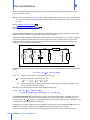
PVSYST V5.0 is a PC software package for the study, sizing and data analysis of complete PV systems.
It deals with grid-connected, stand-alone, pumping and DC-grid (public transport) PV systems, and includes
extensive meteo and PV systems components databases, as well as general solar energy tools.
This software is geared to the needs of architects, engineers, researchers. It is also very helpful for educational
training.
PVSYST V5.4 offers 3 levels of PV system study, roughly corresponding to the different stages in the development
of real project:
-
Preliminary design 17 : this is the pre-sizing step of a project.
In this mode the system yield evaluations are performed very quickly in monthly values, using only a very few
general system characteristics or parameters, without specifying actual system components. A rough
estimation of the system cost is also available.
For grid-connected systems, and especially for building integration, this level will be architect-oriented,
requiring information on available area, PV technology (colours, transparency, etc), power required or desired
investment.
For stand-alone systems this tool allows to size the required PV power and battery capacity, given the load
profile and the probability that the user will not be satisfied (("Loss of Load" 191 LOL probability, or equivalently
the desired "solar fraction").
For Pumping systems, given water requirements and a depth for pumping, and specifying some general
technical options, this tool evaluates the pump power and PV array size needed. As for stand-alone systems,
this sizing may be performed according to a specified probability that the water needs are not met over the
year.
-
Project Design 22 : it aims to perform a thorough system design using detailed hourly simulations.
Within the framework of a "project", the user can perform different system simulation runs and compare
them. He has to define the plane orientation (with the possibility of tracking planes or shed mounting), and to
choose the specific system components. He is assisted in designing the PV array (number of PV modules in
series and parallel), given a chosen inverter model, battery pack or pump.
In a second step, the user can specify more detailed parameters and analyse fine effects like thermal
behaviour, wiring, module quality, mismatch and incidence angle losses, horizon (far shading), or partial
shadings of near objects on the array, an so on.
For pumping systems, several system designs may be tested and compared to each other, with a detailed
analysis of the behaviours and efficiencies.
Results include several dozens of simulation variables, which may be displayed in monthly, daily or hourly
values, and even transferred to other software. The "Loss Diagram" is particularly useful for identifying the
1
Chapter 1 Overview
1
Overview
weaknesses of the system design. An engineer report may be printed for each simulation run, including all
parameters used for the simulation, and the main results.
A detailed economic evaluation 102 can be performed using real component prices, any additional costs and
investment conditions.
-
Measured data analysis 169 : when a PV system is running and carefully monitored, this part (located in the
"Tools" part) permits the import of measured data (in almost any ASCII format), to display tables and graphs of
the actual performances, and to perform close comparisons with the simulated variables. This gives a mean
of analysing the real running parameters of the system, and identify even very little misrunnings.
-
In addition, Tools 131 include the databases management - for Meteo data and PV components - as well as
some specific tools useful when dealing with solar energy systems: import of meteo data from several
sources, tables and graphs of meteo data or solar geometry parameters, irradiation under a clear day model,
PV-array behaviour under partial shadings or module mismatch, optimizing tools for orientation or voltage, etc.
Tutorials
There are presently 3 available tutorials, about the following topics
Meteo data management 104 (import from external sources)
Project design
24
(complete elaboration of a project)
3D near shadings construction
49
Tips for beginners
Help : you can get contextual Help from almost anywhere in the software, by typing F1, or very specific information
are often available with little question mark buttons.
Red dots : every time you have red dots on graphical views, you can drag them with the mouse to modify the
involved parameter (examples: horizon line, plane orientation, near shading orthogonal drawings).
Exporting tables : all result tables can be exported to other software by choosing "Export" in the menu:
- either as text file (ASCII CSV format),
- or by "Copy as text" into the clipboard (to be pasted for example in a spreadsheet software),
- or by "Copy as image" into the clipboard.
For some scrolling tables (solar parameter, meteo), you can choose the time period to be exported.
Exporting graphs : all result graphs can be exported to other software by choosing "Export" in the menu:
- either as image file (BMP color format)
- or by "Copy" in the clipboard, which can be "Pasted" within any other software (MS-Word, etc.).
Current window image: as in all Windows applications, pressing "Alt + PrintScreen" copies the current window
into the clipboard.
Printing tables, graphs or other components: 182
- allow for a double line comment in front of each print form,
- are usually "intelligent" printings which hold complementary useful parameters,
- offer a "preview" facility,
- often ask for desired details about outputs,
Screen resolution:
PVSYST has been developed and optimised using the standard SVGA (800x600 pixels) screen resolution
with small fonts.
Using old VGA (640x400) is not advised: it will superimpose all dialog windows, hiding the "historical" tree of
window labels indicating where you are presently located in the software.
With higher screen resolutions; you are not advised using large fonts, which can produce unexpected display
effects as the software was not quite tested for them.
For changing the screen resolution, please open the msWindows tool "Display settings". You can usually
reach it by right-clicking the windows main screen, and choosing "Properties".
Chapter 1 Overview
2
Overview
1
Historical evolution of the software
Of course any newly discovered bug (and bugs reported by the users) are repaired for each new version.
Also the contextual "Help" system is continuously updated, either concerning new developments, or according to
the numerous questions of users.
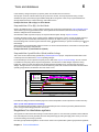
Version 5.3 (November 30th, 2010) by respect to Version 5.21 (September 3rd, 2010)
1. Help system: completely new CHM version, now fully compatible with Windows 7.
A PDF version is available on the site.
2. New tool for the Meteo data quality check (Kt plots, clear days check)
3
4.
5.
6.
7.
8.
9.
Implemented middle-interval shift for optimizing treatment of not-centered meteo data
Importing meteo data from Global Incident (POA) measurements: bug fixed
POA measured value now in the recorded data
Concentrating PV module (CPV): definition with spectral corrections
Concentrating systems: complete revision of the simulation process / variables
Update of the loss diagram, also for concentrating systems.
Inverter definitions, some bugs fixed: 3-voltage reading, bi-polar sizing,
Heterogeneous fields: old files V 4.37 prevent simulations (0 everywhere)
IAM calculation on diffuse: also with customized IAM function
Version 5.21 (September 3rd, 2010) by respect to Version 5.20 (August 3rd, 2010)
1. Direct link for importing PV modules and Inverters from PHOTON database
2. Shadings: define a new object (mansard, or roof-window)
3. Favorites choice in the main Database lists easier (by right click).
4. Directory Names now accept accents and some special characters
(solving problems with Czeck Republic Windows XP installations).
5. Meteo data: the wind speed is now part of hourly values when defined monthly.
6. Inverters: still problems with 3-voltage efficiency definition (solved).
7. Sun-shields: bug during mutual shading calculations
8. Fixed littles bugs: printing of PR, soiling table in parameters, etc.
Version 5.20 (August 3rd, 2010) by respect to Version 5.14 (June 30th, 2010)
1. File organization and localization has been changed
Your working \Data\ structure is now in a writable area
(avoiding delocalization of files written by PVsyst under Vista and Win7)
2. Module layout tool for the geometrical arrangement of your system
3. SolarEdge architecture: special option for decentralized architecture with Powerboxes.
4. Fixed bugs in Inverter definition, Projects, Latitudes over polar circle, etc.
Version 5.14 (June 30th, 2010) by respect to Version 5.13 (June 25th, 2010)
1. On some machines, for unidentified reasons (firewall, proxy, ?)
the AutoUpdate function induces crash at the opening of the software
Version 5.13 (June 25th, 2010) by respect to Version 5.12 (May 25th, 2010)
1. Autoupdate: freezing at opening on some Windows installations (web access)
2. AC loss: now possible after inverter or after external transfo
3. AC loss: bug when identifying mono/tri situation
4. Heat loss default values: bug, not always possible to change value.
5. Stand-alone, economic evaluation: bug fuel consumption
6. Stand-alone, Available energy and Time fraction: bugs when very bad design
7. Simulation: Bug Hourly plots for some variables.
3
Chapter 1 Overview
Overview
1
Version 5.12 (May 25th, 2010) by respect to Version 5.11 (April 27th, 2010)
1. PV modules definition:
- shows the apparent Series resistance (Rsapp, different from Rsmodel)
- Efficiency plots vs. irradiance: display low-light values
- Improved parameter definition in the help
2.Still bugs for the automatic update (freezed the program in some cases)
Version 5.11 (April 27th, 2010) by respect to Version 5.1 (April 16th, 2010)
1. Thermal U value default definitions for some typical situations
2. Bug shed shadings, new feature according to modules
3. Load definition: lowered low limit to less that 0.05W.
4. Auto Updates should be operational from next version.
Version 5.11 (April 16th, 2010) by respect to Version 5.1 (March 25th, 2010)
1. Bug when importing some meteo data (PVGIS and Helioclim)
2. Animation video file (*.avi) compatible with Windows media Player
Version 5.1 (March 19th, 2010) by respect to Version 5.06 (January 26th, 2010)
1. Automatic auto-update for new versions (doesn't work well until V 5.14)
2. Tool for the analysis of electrical effect of cell shading:
Extended to several cells, in one or several sub-module (groups protected by one by-pass diode).
3. Generic (unlimited) shed shadings: electrical effect of shadings on the first cell row and bottom string.
4. Mismatch: histogram for the statistical study of loss distribution.
5. System design reference temperatures: now part of each project.
6. 2-axis tracking: shadings compatible with concentration option.
7. Help: tutorials for project design and meteo data.
8. F10 key for directly switching english <=> local language in most dialogs.
8 Helioclim data: updated tool according to the new web site data format.
9. Defined bi-polar inverters in the system design and simulation
10. Inverter: bug when efficiency not well defined
11. Heterogeneous fields: still bugs in area calculations and mixed fields.
12. Video recording of the shading scene now works
13. Stand-alone systems: bugs in regulator definitions and system verifications
14. Array voltage was not registred in the simulation
15. Export project tool: error warning, corrected
Version 5.06 (January 26th, 2010) by respect to Version 5.05 (December 18th 2009)
1. PV model: Saturation current Io limit down to 0.1 pA (equation problems at low temperatures).
2. Helioclim data: the provider of these data has modified the site's format
=> readapted the program for a compatible easy importation
3. Shading calculations sometimes freezed. Improve reliability of shading calculations.
4. Near shadings, elementary objects, autorized tilt < 0°.
5. System dialog: did not keep the defined parameters when re-entering the dialog.
6. Inverter database: terminated the update according to Photon Magazine 2009.
7. Vista and Windows 7 compatibility: Parenthesis were not allowed in the directory \program files (i86)\
proposed by Windows.
Version 5.05 (December 18th, 2009) by respect to Version 5.04 (November 24th 2009)
1. Stand-alone systems: bugs in the Regulator dialog and the simulation process
2. Grid system sizing tool: still another deep revision for more conviviality
bugs with master/slave definitions (sometimes divisions by 0)
possibility of Strongly Oversized inverters (by modifying Hidden parameters)
Chapter 1 Overview
4
Overview
1
3. Inverter for 3 voltages: still some little improvements
Version 5.04 (November 24th, 2009) by respect to Version 5.03 (November 10th 2009)
1.
2.
3.
4.
5.
Hidden parameters were not modifiable (bug).
Regulator definition had intempestive warnings, preventing using it.
Heterogeneous fields: compatibility and warnings Orientation <=> Shadings
Tracking frames with N/S frame: the tilt limits were not active
Inverter database: partial update (about 30%) from Photon Magazine 2009
Version 5.03 (November 2009, 10th) by respect to Version 5.02 (October 2009, 26th)
1. Corrections in the Grid-system sizing tool (MPPT inverters, not yet perfect !).
2. Some background colors make things unreadable in Vista and Windows 7.
Version 5.02 (October 2009, 26th) by respect to Version 5.01 (October 2009, 12th)
1. System definition freezed when defining multi-MWc systems. No more limit to the system size.
2. Improved the system sizing tool.
3. Corrected further bugs in the report (sometimes over-printing at head of the page).
4. Improved the ordering tool (sometimes e-mails were not well sent, and we did not receive your order).
Version 5.01 (October 2009, 12th) by respect to Version 5.0 (October 2009, 6th)
1. We just discover a important bug: in some cases (synthetic generation without specified Diffuse monthly
values), the Diffuse is very low, leading namely to over-estimated transposed values (GlobInc). Please
reinstall this new version, and open the projects elaborated under V 5.0. If this occurs, the program will give a
warning, re-calculate the meteo file, and you should re-simulate all your calculations for this project. Please
discard the old inputs of such erroneous projects.
2. Help improved for system design and inverter sizing.
3. Bugs in the report of the Heterogeneous multi-orientation fields
4. Module database completed for all modules references in Photon Magazine 2009 (now about 5'300
modules).
Version 5.0 (September 2009) by respect to Version 4.37 (June 2009)
This is a major modernization of the software. Many internal mechanisms have been improved since more than 2
years of development (in parallel to version 4.xx updates). Therefore there may be bugs which have not been
detected during the development. Please be so kind as to report them carefully to the authors.
1. Multilanguage: the simulation report was already available in several languages, but now the software itself is
(partly) available in English, French, German, Italian, Spanish and Portuguese.
This is not yet a full translation: only the most used parts - especially regarding grid connected systems - were
translated up to now. This is a very time-consuming job (more than 200 dialogs, and hundreds of information/
warning pieces to the user), and we will continue it progressively. On the other hand we don't intend to
translate the Help at the moment.
2. Multi-fields: you have now the opportunity of defining several field types for a given project (with different PV
modules or inverters, number of modules in series, etc). Their parameters are detailed on the final report, but
the simulation results concern the whole installation.
3. Inverter: their definition includes many parameters which were not operational in the simulations up to now.
Multi-MPPT devices: you can define a specific sub-field for each input.
Possibility of Master/Slave operation: the Inverter's cascading is taken into account in the simulation
process.
For some models: power limitation when running under a specified input voltage, is now taken into account.
Efficiency profile for 3 different input voltages.
4. Heterogeneous orientations: systems with 2 different orientations may now involve different sub-fields in
each orientation, and/or a subfield for which the strings of a given inverter are distributed on both orientations
(with mix of the I/V curve for correct calculation of the MPP).
5. Database management: the big lists of components stored as individual files, which took very much time to
be loaded in the previous version (and sometimes caused bugs) are now replaced by centralized databases
(CSV files). This results in an immediate access, and facilitates the updates of the DB of the software. Only
the files you are creating or modifying by yourself will still be stored as individual files as before. This
5
Chapter 1 Overview
Overview
1
concerns:
The PV modules (which should approach 5'000 modules in the DB of 2009),
The inverters,
The geographic site database 5of which the lis shows now the source of data).
6. Favorites: you can now define a list of your favorite components in the database, which drastically simplifies
the use of big component lists.
7. Near Shadings: the full dialog and tool have been improved. You can now:
Easily read and write a scene or a building directly from the 3D tool.
Multiple selection allows to define groups of objects, that you can replicate or save on a file.
Define/fix the characteristics of the view you would like to appear in the final simulation report.
Register the shading's animation as a little video.
8. Special tracker devices with PV modules rotating on a tracking frame (with either N-S or E-W axis), are defined
as special shading objects (with database of existing devices).
9. Shading of thin objects, like electrical wires or handrails, is now possible by weighting their effect on the
"Module shading" part of the shaded areas.
10. Shading on strings: you can put a weight on the effect of the shading according to strings, in order to better
approach the real shading effect on the electrical production (not only an upper limit) in the simulation.
11. Import Horizon profiles directly from Somletric SunEye, Carnaval software, Meteonorm.
12. Synthetic hourly data generation: the diffuse part may be renormalized to specified monthly data when
available. This was not possible in the previous versions.
13. Improvement of the sizing tool for grid systems.
You have now the opportunity of specifying either the nominal power, or the available area as starting point.
The software indicates the required ranges for the number of modules in series and in parallel.
A new powerful window shows all the constraints when sizing a field, i.e.
The voltages of the operating array by respect to the inverter's specifications,
Histogram of the waited power production of the array, compared to the inverter's nominal power.
Estimation of the overload losses (and visualization of their effect on the histogram).
This tool allows to determine precisely the ratio between array and inverter Pnom, and evaluates the
associated losses.
14. The default losses management has been improved, especially the "Module quality loss" which is determined
from the PV module's tolerance, and the mismatch on Pmpp which is dependent on the module technology.
15. Losses between inverters and grid injection have been implemented. These may be either ohmic wiring
losses, and/or transformer losses when the transformer is external.
Version 4.37 (June 2009) by respect to Version 4.36 (April 2009)
1. Changed the program for the installation. The old one was no more compatible with the new ServicePack 3 of
Windows.
Version 4.36 (April 2009) by respect to Version 4.35 (March 2009)
1. CdTe modules: the module definitions of the old database are affected by the new recombination losses.
=> Recreated files in the database for all CdTe modules, including recombination term according to our
recent measurements at the University of Geneva.
Version 4.35 (March 2009) by respect to Version 4.34 (Feb. 2009)
1. Import of Meteo data:
Bug in some new files of Meteonorm V 6.0 (containing leap years)
Bug in some TMY3 files (date recognition)
2. CdTe PV modules: according to our detailed measurements: opportunity of defining Recombination Losses.
3. Shading factor calculation (especially diffuse): bug when the plane azimuth is very unusual (north in Nordern
hemisphere).
Version 4.34 (February 2009) by respect to Version 4.33 (Sept. 2008)
1. Database: PV modules from manufacturers (especially many amorphous) and new inverters.
2. Tool for analysing shading of one cell in an array: Improvements, shows now shaded I/V charact. and Pmpp
Chapter 1 Overview
6
Overview
1
loss.
3. Meteo data import:
US-TMY3
Import implemented (1020 stations available)
Satellight:
Bug temperatures when importing 5 years at a time.
PVGIS: Bug all months accounted as 31 days (overestimate 1.6%)
PVGIS: Now uses PVGIS site new interface, much more convivial
Meteonorm:
Monthly files: still discovered a new format variant
Temperatures: Possibility of importing NASA data, always available.
4. Tracking tilted axis: error when axis azimuth not south.
5. Measured and Meteo data: little bugs (extended available date formats).
Version 4.33 (September 2008) by respect to Version 4.31 (July 2008)
1. Database: PV modules update from Photon Magazine 2008 and other manufacturer's data (over 3100
modules in the DB)
2. Loss diagram: still an error in the GlobShd evaluation (but doesn't affect the final results)
3. Meteonorm import: tolerant to another (not yet registred) file format
Version 4.32 (July 2008) by respect to Version 4.31 (June 2008)
1. Database: Inverters update from Photon Magazine 2008
2. Loss diagram: incoherences in the shading and IAM relative losses (only display in this diagram - simulation
results were correct)
3. Ascii Meteo importing tool:
Date management improvement,
Site names beginning by "New" are now possible.
4. Search Edit for easier choice in big component lists.
5. Print Preview: easier navigation through pages.
Version 4.31 (June 2008) by respect to Version 4.3 (March 2008)
Some bugs fixed :
1. Satellight data import: Temperatures were not well imported.
2. PVGIS import: copy/paste did not work with some internet browsers.
3. Site/Meteo choice for Projects: generated erroneous meteo files
4. Simulation report: erroneous tables overwrited parameters (namely IAM)
5. Import of Meteo ASCII files: improvements for daily data and date formats.
6. Long component's lists: edit box for direct access to a given item
Version 4.3 (March 2008) by respect to Version 4.21
1. Import of meteo data from multiple popular sources (NASA, WRDC, PVGIS, RetScreen, Helioclim).
2. Comparison between several Meteo Data sources. Developments and results in the Help.
3. Import/Export of "Site" monthly data from/to EXCEL.
4. Improvement of the Meteo hourly files management (site and comment now editable/exportable).
5. Implementation of Tracking with vertical axis, also useable with positioning of modules on a "dish"
6. Module temperature calculation: revision (new parameters, absorption, etc).
7. PV model for amorphous: parameter determination according to a specified muPmpp value. Adjusment of all
triple-junction module parameters in the database.
8. Bug Tracking: azimuth sign error in south hemisphere: the tracking was reversed !
9. Bug Shadings, polygonal fields: rewritten the whole modules calculation.
Version 4.21 (September 2007) by respect to Version 4.2
No new developments, only corrections of bugs. The main ones were:
1. Tracking two axis: returns to Azim=0 when sun over +/-90°.
2. Near shadings: verification of interpenetration field-objects, some editing errors or improvements
7
Chapter 1 Overview
Overview
1
3. New PV modules didn’t appear in the list.
4. Simulation: sometimes division by 0 with sheds.
5. Project situation dialog: improved copy of site <=> meteo.
6. Graphs: copy of the curve values to clipboard for exporting.
Version 4.2 (July 2007) by respect to Version 4.1
1. Improvement of the navigability in the 3D construction tool, copy/paste of an object from one variant or project to
another one. Automatic verification of the Field interpenetration (or tangency) with another object, which may
prevent good shading calculations.
2. Backtracking strategy with all tracking systems, involves tracker width and distance definitions.
3. Sun-shields definition in the 3D tool; also with backtracking, which may considerably improve the sun-shield's
performances.
4. High-Concentrating systems simulation, associated with 2-axis trackers; adaptation of the simulation process
and loss diagram.
5. Long-term financial balance tool, including several Feed-in tariff strategies (day/night or seasonal variations,
feed-in and self-consumption tariffs, etc) and system ageing.
6. Soiling parameter included in the simulation and loss diagram, with opportunity of defining monthly variations.
7. Direct import of meteo values from NASA-SSE database over the whole earth (by 1°x1° cells), and practical
procedure for importing meteo values from WRDC database, especially for countries where METEONORM data
are scarce.
8. Improved the model for amorphous PV modules, especially safety of parameter boundaries, and behaviour
presentation to the user.
9. Improved the Project dialog and choice of a site/meteo. Improved compatibility checks between the project's
site and hourly meteo. Extraction/edition of the site geographic properties within an hourly meteo file, which was
not possible up to now.
10. Database update, with PV modules and inverters of 2006/2007 (now around 2250 PV modules and 770
inverters).
11. Adaptations for Windows VISTA OS, especially concerning the visual interface. All other functions seem to be
perfectly compatible.
12. Introduction of many "Logs" in the program, in order to facilitate the debugging of user's problems.
Version 4.1 (January 2007) by respect to Version 4.0
1. MultiLanguage
The Simulation output reports are now available in French, German, Spanish, Italian (useful for presenting the PV
system characteristics to customers).
Please contact the author if you wish to implement yourself a translation into your own language (you should have
a good knowledge of the technical terms used in the PV technology).
2. Windows user's rights compatibility
The DATA structure has been modified for compatibility with the user's rights protections in Windows. A user
without writing rights can now copy the whole DATA structure for use in his own writable area. Data may be
shared - or not - between different users of the machine.
3. Files and projects transfers
Archiving or importing projects, as well as database updating tools have been improved.
4. Bugs in special shading parts
Several "youth" bugs in newly developed features (often on special requests of users) have been fixed. Especially
in the Shading part, concerning tracking mechanism as well as sheds with a tilted baseline or double-orientation.
Version 4.0 (June 2006) by respect to Version 3.41
The main new feature in this PVsyst 4.0 version is the study of Pumping systems, which involves complex
developments which may be not quite safe in this first issue.
1. Pump Model
Development of a general and original pump model, suitable for use in PV applications.
Chapter 1 Overview
8
Overview
1
This should be suitable for any type of Pump or Motor useable in PV systems.
This should describe the operating of the pump over a large Electrical and Hydraulic domain, encountered in PV
conditions.
Its parameter should be available from usual pump manufacturer's datasheets. For a given pump, the model may
be specified using several kinds of original data.
Its accuracy over the whole domain has been checked for some pumps using measured data.
The defining dialog shows graphics of the behaviour of the model, as functions of all relevant variables.
The pumps database is still limited to about 20-30 models; only one manufacturer has answered our request for
datasheets…
2. Controller / Converter device for pumping
Model for a new controller for pumping systems, including the System Configuration controls and Power
converter.
A default controller is proposed for each system configuration, with parameters automatically adjusted according
to the system for optimal operation.
3. Pumping systems
Three system types are proposed: Deep well, Pumping from lake, pond or river, and Pressurisation system;
For each type, several system configurations are possible: Direct coupling (with eventual improvements like
booster, pump cascading or array reconfiguration), with Power converter (MPPT or Fixed V), or battery-buffered.
Water needs and Head characteristics may be defined in yearly, seasonally or monthly values.
4. Presizing tool for Pumping systems
As for stand-alone systems, a Pre-Sizing tool has been developed, which proposes a PV power and Pump
power sizing, according to the location and meteo, user's needs and LOL requirements. This simplified model
takes the pump technology and system configuration into account. It also proposes a very rough estimation of the
costs.
5. Detailed Simulation
The design of the pumping system - rather complex with such a number of pumps and system technological
aspects - is assisted by numerous sizing propositions, and helps (advices, graphs, blocking of uncompatibilities,
etc) when choosing the system layout and configuration.
The hourly simulation accounts in detail for all features defined for the system, and is specific for each
configuration listed above (direct coupling, with converter or battery).
As for the other systems, a detailed engineer report explains all parameters and results of the simulation. All the
losses and mismatches along the system are quantified, and visualised on the "Loss Diagram", specific for each
configuration.
6. Help for pumping systems
The development of this Pumping tool has brought a deep understanding of the PV pumping systems
problematic, and the operating / efficiency limitations inherent to the numerous possible solutions.
This Help describes in detail the implemented models, and sets a broad panel of the different available
technologies, as well as delimits their implementation boundaries.
7. Heat transfer factor for thermal losses of PV array
Some users has pointed out that the proposed parameter accounting for wind velocities was not correct and lead
to underestimated thermal losses. There is a new detailed discussion on this subject in the Help, and the
program now advices to use wind contribution only when the wind velocity is quite well determined (now default
value is Kv = 0 W/m²K / m/s)
8. Inverters
Several parameter usually specified in the datasheet have been added to the inverter definitions. But none of
them is used in the present simulation. Refinements of the inverter modelling are planned for a next version.
These new data have been added in the whole database when available. Almost 300 new inverters were
introduced, many also suited for US market. The database includes now more than 650 inverters.
The 50/60 Hz frequency has become a choice criteria in the lists.
9. PV modules
The choice list shows a nominal (MPP) voltage of each module for making the system design easier.
9
Chapter 1 Overview
Overview
1
The database includes now more than 1'600 PV modules.
The PV module definition dialog was improved and some bugs fixed.
Specifying the Voltage or Power Temperature coefficient is now possible also for amorphous modules.
10. Remarks in PV components
An unlimited text editor is now available for giving detailed descriptions of all the PV components.
11. Miscellaneous improvements or fixed bugs
- Projects are now sorted according to their system type in the list.
- The "Archive Projects" tool has been debugged and improved.
- Summer/Winter Hour may now be taken into account when importing Meteo Data as ASCII files.
- Some little bugs concerning the simulation, especially of stand-alone systems (Wearing state not computed,
display errors, etc).
- Loss diagrams: complete review, some corrections for losses coherence.
Version 3.41 (March 2006) by respect to Version 3.4
1. Automatic facility for importing "satellight" meteo data.
"Satellight" data are real measured meteo data, available free from the web for any pixel of about 5x7 km² in
Europe, and for years 1996-2000. Their quality becomes better than any terrestrial measured data, as soon as
you are far from more than 20 km of the measuring station.
2. Fix some bugs of version 3.4, concerning:
- HIT PV modules model,
- memory leakages and orientations in some shading special cases,
- transposition safety when bad meteo values,
- orientation choice dialog,
- meteo ASCII conversion facility.
Version 3.4 (July 2005) by respect to Version 3.3
1. New modelling procedure for the amorphous modules
This procedure was established and validated using the results of a research project performed at CUEPE,
funded by the SIG-NER fund (the SIG - Services Industriels de Genève - are the Geneva Electric and Gaz Utility).
This project included detailed long-term measurements of 6 PV modules in real conditions. It also gave a
quantified validation of the standard model for crystalline and CIS modules.
2. Extended component database
Over 1'200 PV modules and 400 inverters are now referenced, with dates for identification of market availability or
obsolete components. With such big lists, a mechanism for quick access time (and background process update)
had to be implemented.
3. Near shading 3D tool
View of the shading scene in realistic colors (settable by the user for each object) - instead of "iron wires"
representation - improves the understanding of complex scenes, and gives a much more attractive image of the
project for the final customers. Animation over a whole chosen day also clarifies the shading impact of a given
situation.
4. Implementation of tracking planes in the 3D shading tool.
Especially suited for the optimisation of heliostat arrays layout.
5. Review and improvement of the Simulation Process
Clarification of the losses at any stage of the system, extension to battery systems with DC-DC converters,
rewriting of the heterogeneous field treatment , etc.
6. Detailed loss diagram
Gives a deep insight on the quality of the PV system design, by quantifying all loss effects on one only graph.
Losses on each subsystem may be either grouped or expanded in detailed contributions.
7. Restructuration of the internal representation of the physical variables
These two last improvements were made possible thanks to a very deep revision of the internal data structure, in
Chapter 1 Overview
10
Overview
1
order to obtain more flexibility when using the simulation variables. This reorganization is transparent for the user,
but allows now many enhancements of the simulation process, namely easy adding of new variables when
necessary, including them dynamically in the simulation process according to specific system configurations (for
example defining regulator losses when used in a battery system), or inversely discarding other ones when they
are not relevant.
The old fixed variable set did not allow a coherent description of the system losses. Therefore simulation has to
be performed again for getting the Loss Diagram on the old result files.
Caution: In spite of intensive tests, these deep modifications may have produced some bugs which have not
been detected by the author. We thank the users for carefully reporting any misrunning or strange behaviour of the
software to the author.
8. Measured data – simulation comparison
Improvement and debugging of the Measured Data Importing Tool, and the comparison between measured and
simulated values. Improvement of the break-down data eliminations.
9. Daily and Hourly Plots of the load profiles
Version 3.3 (February 2004) by respect to Version 3.21
1. Output results presentation and hourly plots
When displaying simulation results, the standard printable result forms are now directly accessible (while they
were only available through the "preview" option in the "print" dialog up to now).
During simulation process, the program can store a sample of chosen variables in hourly values. This allows for
displaying graphics in hourly or daily values, with several variables on the same plot.
Thanks to a very fast and easy navigation over the whole year, this offers a powerful tool for visualizing the
instantaneous behaviour of the system all over the year. This helps, for example, identifying unexpected
behaviours of the system in some specific operating conditions (for example, SOC and regulation states in standalone simulations).
2. Stand alone systems: implementation of MPPT and DC-DC converters
Up to now the stand-alone systems were only defined with a simple usual configuration (i.e. PV array directly
connected to the load and battery through the regulator).
It is now possible to include a MPPT or DC-DC converter between the PV array and the battery/load. This converter
is part of the regulator definition.
3. New tool for optimising Fixed Input Operating voltage
Shows the average power or efficiency of the PV array over a period (year, summer, winter), as a function of a fixed
user's voltage. Shows ohmic and diode voltage drop effects.
4. Hourly profile for domestic use load definition
In order to better estimate the battery behaviour and wear. Automatic placement of lighting and TV uses to evening
hours.
5. Improved irradiance clear sky models for very high altitudes (up to stratospheric).
For very special uses of the software.
6. Meteonorm input adaptation
The outputs format of the Meteonorm monthly files has been changed with the new version 5, and we had to
match the reading format accordingly. This is not yet quite fixed (namely the new Meteonorm files don't include the
Station name nor the geographical coordinates, which have to be input manually).
6. Databasse update
Added about 500 new PV modules, from the PHOTON magazine tables of February 2003 and February 2004.
Added about 40 Inverters from PHOTON magazine, march 2003.
Created a list of the main component manufacturers. This list is now selective, according to Manufacturers/
Retailers and Component type.
Version 3.21 (November 2002) by respect to Version 3.2
11
Chapter 1 Overview
1
Overview
Shading factor calculations with partition in Modules chains: Some computation errors had been introduced with
v3.2, fixed.
Horizon definition with more than 20 points now possible.
Minimization (iconisation) of the Program window now works.
Corrections for compliance with Windows XP environment.
Version 3.2 (July 2002) by respect to Version 3.11
1. Thin film modelling
The main novelty is the special tools for the treatment ofThin film technology modules
tripple junctions, CIS, CdTe).
141
(a-SI:H, with tandem or
Up to now the program used the standard one-diode model, although it is not well-suited for these technologies.
There is no consensus up to now in the PV community on how to model these devices. The task of finding a
general model is by far above our possibilities. It would require a big research project at the international level).
Nevertheless we carefully measured a single device in great detail (a-SI:H tripple junction) and tried to find
improvements of the "standard" one-diode model. We found and implemented two adjustments, which can
improve significantly the performances of the model:
- the Shunt resistance of the device is drastically increasing (exponentially) when the irradiation diminishes.
- the temperature behaviour, which is fixed as a result in the standard model, can now be adjusted at any desired
value (often given by manufacturer).
For our test device, this diminished the modelling error (over a 4-month continuous measuring period) from about
11% to a very few (1 to 3%). But this doesn't take spectral effects into account (see the "Help" for further details).
Be aware that these are available tools, but we cannot assess parameter values for any modules or any
technologies.
2. Orientation optimising tools
There is now an on-line tool showing the collecting performance as a function of tilt and orientation when
choosing them.
Also for shed disposition, a new graph shows the annual yield curves taking shadings into account, for
optimising the tilt, shed spacing and collecting/ground area ratio.
3. Components Database tools
Export and Import of PV components (PV modules, Inverters) between the PVsyst database and spreadsheets
like MS Excel, allowing for displaying, input and correcting component data in tabular form.
Improved and securised default values for the input of new PV modules in the database, only based on
Manufacturer datasheets. The Excel sheet shows clear detailed information about required, optional and PVsystcalculated parameter.
Inverters: Automatic build of efficiency profile, according to Maximal and "Euro" efficiency data. This allows for a
much more easy input of inverter data from Manufacturer datasheets.
Be aware that due to additional parameter, PV module and Inverter files written by Version 3.2 are not yet readable
with anterior versions (but old files can of course be read by version 3.2 !).
Update of the Database, which includes now more than 600 PV modules and 200 inverters of the market.
4. Miscellaneous
Near shadings: several little bugs and practical improvements. Improved the tools for manipulating and zooming
the scene on the screen. Implemented the display of shadings calculated by points, when standard polygon
algorithm fails.
Included a full example as tutorial for the "Measured Data Analysis" part, which allows for importing measured
data in PVsyst, and closely comparing them with the simulated values.
Revision and improvement of the "PV array behaviour" graphic tools. Included a detailed Help.
"Perez" transposition algorithm (not the Hay transposition model proposed by default !) had a little bug which
caused a discrepancy of the order of 2-3% on yearly results for vertical planes (and of course less for less tilted
planes).
Revision of the tool for defining Currency Rates, which had some bugs.
Chapter 1 Overview
12
Overview
1
Revision of the general displaying conditions when using screen settings with "large fonts". Many windows
appeared not full developed, and had often to be resized. Also graphics and tables had sometimes very little
fonts.
Reading of files without "Archive" attribute (which is sometime removed by some file managers) is now possible.
Version 3.11 by respect to Version 3.1
Meteo: generating meteo hourly files in CSV format for export.
Meteo transposition tables: possibility of -180°..180° scale.
Horizon: automatic import of files from "Meteonorm" and "HoriZON" software.
PV module: Pnom tolerance from manufacturer included as parameter.
Simulation: The user can now define a PV module quality loss, by respect to the manufacturer nominal data on
which is based the PV module model. Therefore the results can be adjusted if necessary for Energy Yield
Warranty.
Installations in Polar regions: Possibility of defining meteo, and performing pre-sizing and simulations for Arctic
and Antarctic meteo (including months with zero irradiation).
Version 3.1 by respect to Version 3.01, 3.02 and 3.03
Database updates will be periodically available on the WEB site www.pvsyst.com. A special tool allows to
dispatch the files into the PVSYST data structure.
Printed outputs: Printed results forms may also be exported as image, for pasting in other software like MS-Word.
Allows to fully insert PVSYST results in documents (useful for example for sending them by e-mail).
Import of Meteo data: Import from Meteonorm software now quite debugged (except for bugs of the Meteonorm
software itself with monthly data: the program tells you how to come over).
Direct import of US TMY files (240 US sites available free from WEB).
User's needs definitions: Graphs and printings are now available. A new feature allows for importing Load
Profiles in hourly or daily values from ASCII files (e.g. for example from EXCEL).
Horizon definition: Diffuse and Albedo factors are newly introduced.
Horizon treatment in simulation strategy has been changed: it is now equivalent to the near shadings treatment (i.
e. included in the "shading loss" calculation).
Near Shading tool: Further debugged. Undo facility (up to 10 levels), Very useful new tools for distances and
angle "measurements" on the scene.
Simulation: Losses: New parameter accounting for the real quality of PV modules.
South hemisphere compatibility: Fully debugged, with new azimuth definition (negative toward east, clockwise).
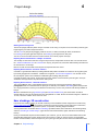
Sunpath diagrams are now from right to left (negative azimuts, i.e. sunrise, are on the right of the graph, as the
sun progression ...). Therefore gives realistic image of the horizon drawing.
Measured data: Importing widely debugged, Possibility for ASCII lines of more than 255 characters, Data import is
now possible with input Daily Values. Measured data with orignal irradiation measurements in the collector
plane. Graphics and comparison tool are debugged and improved.
Version 3.0 (December 1999) by respect to Version 2.21
The PVsyst software has been entirely rewritten, using the Borland DELPHI 3 platform instead of the old
Borland Pascal 7, gaining in user graphical interface quality and reliability, as well as in compatibility with most
recent versions of the Windows operating system.
The user's interface has been redesigned, and navigation in the software was strongly improved, with the
collaboration of the LESO-EPFL team. Introduction of a "Green line" for guiding the user in the project
development.
Preliminary design: Implementation of this quite new sizing feature, for grid-connected and stand alone systems.
Project design: The Project organization has been simplified. Parameter definition and results are summarised
in one only "Simulation Version" file. Several valuable tools were added (including the sizing "expert" for building
the system parameter).
13
Chapter 1 Overview
1
Overview
Several new Tools which help understanding more deeply many PV system behaviours.
"Help" system, which provides a detailed contextual "help" by typing F1 anywhere in the program.
Compatibility and Troubles
This software is now available in several languages (English, French, German, Italian, Spanish, Portuguese).
Additional languages could be included by filling the files "Texts.csv". But the languages using other Character
sets than the standard ANSI may cause great difficulties.
PVSYST V5.0 runs under any Win'95/'98, Windows NT or 2000, Windows XP, Vista (32 bits) and Windows 7.
Most of the data files from PVSYST, versions 3.xx and 4.xx (projects, components, meteo) can be read with this
new version 5.0. But the inverse is not true (upward compatibility).
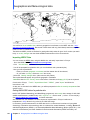
Importing Meteo Data:
- Link for direct import from the Meteonorm 117 software (versions 4, 5 or 6).
- Link for direct import from many popular meteo data sources 112 from the web (including NASA for the whole
world, US TMY3, PVGIS, Helioclim, Satellight, Retscreen, etc).
- Almost any custom "Hourly Meteo" or "Measured Data" ASCII file can be imported, whenever it holds one data
record on one ASCII line.
Most detailed data (hourly or daily data) produced by the software can be Output to CSV customised ASCII files
(compatible with any spreadsheet program).
Many Data Inputs or Output are possible through the clipboard (graphs or tables as bitmaps, tables as CSV-text
images, allowing direct export to spreadsheet programs like Microsoft EXCEL).
Many input files in ASCII format are accepted, i.e. for measured data, hourly load profile values, horizon profiles,
etc.
Troubles
Many new features have been added in this versioon 5.0. These motivated deep changes in the internal
organization of the software. Although it has been tested in some relevant conditions, it is impossible to check all
the running possibilities after each change in the program.
Therefore the early version 5.0 will probably show weaknesses in the first period. If you encounter some problem
during the use, be so kind as to report them carefully to the authors.
In the same way, if you have some suggestions for improvements or adding some useful new feature, please
don't hesitate to contact the authors !
The "Pumping" part was a quite new development in version 4.0. Owing to its complexity, it was not at the top of
performances in the first version 4.0. It should be progressively improved for the future versions, but we observed
that as it is not used very intensively, we had very few returns of users about its problems.
You can install PVsyst from our website www.pvsyst.com, and install it.
It will work during 15 days without any limitations, for evaluation.
After that it will revert in DEMO mode, and you will need a licence and activation code for using it.
License rights and activation code
License Rights
For new customer, we request that each company, juridical entity, per country (hereafter named company),
to purchase the PVsyst license rights prior to be entitled to purchase activation codes. This price is a one
time fee per company. The set of the PVsyst license rights and the activation code(s) is considered as a
group identified by a Customer ID.
Activation Code
After installation, PVsyst runs in evaluation mode (with full capabilities) during 15 days.
Afterwards, it turns in DEMO mode, and you have to request an activation code
to run the software in unlimited-time mode.
Chapter 1 Overview
16
which will allow you
14
2
Licensing
One activation code per workstation is required. The activation code is paired with the Local Number
resulting of the installation of PVsyst on a given workstation.
Requesting an activation code
16
Upgrade and Update
If you already own a previous version of PVsyst (with a lower major version number, i.e. V4.xx or V3.xx), an
upgrade activation code is required to upgrade to the latest version 5.xx of the software.
One upgrade activation code per workstation is required.
Update of the software, i.e. change to a higher minor version number (e.g. V5.21 to V5.3) is free of
charge.
An automatic tool in the software checks for new version available each time you run PVsyst, and performs
the installation upon user request.
Price list
PVsyst License Rights
Activation Code(s)
Upgrade Activation Code(s)
(V4.xx or V3.xx)
Discount for Academic and
Educational Institutions
800 CHF/ per company
200 CHF/ workstation
100 CHF/ workstation
- 20%
VAT
An additional VAT is charged for Swiss users only. No additional taxes nor shipping costs are required for
all other countries (at least from the exporter point of view).
Transferring the software code to another machine
17
NB: The Activation Code is constructed using the "Local number" provided by each installation of the
software on a given workstation. If you have to reinstall your "Windows" environment, the Local number will
change and your code will no longer be valid. Therefore before reinstalling Windows, you should transfer the
code 17 to another workstation, in order to keep your activation code valid. After reinstalling Windows and
PVsyst on the original workstation, you will be able to retransfer back your code from the other
workstation.
NB: In special cases, people who need to dedicate the code to a given machine whatever the Windows
installation (for example in classrooms machines where windows has to be reinstalled frequently), you can
get another type of License code, based on the Hard Drive number. Nevertheless this code cannot be
transferred to another machine.
Network
Installation on a network server is not recommended. Nevertheless, it is authorized only if each user
computer has a valid activation code.
Please note that this software has not been fully tested for this mode of operation.
But you can share your data area in network with other users.
For this please open "Files" / "Directories", and here you can copy your working space \ Data \ anywhere
on your machine. If you have to put it on a network, please consider your network path as a disk, as
PVsyst doesn't recognize the network \\: paths.
Be aware that no check is performed for the simultaneous use of data.
15
Chapter 2 Licensing
Licensing
2
Warning
Neither the University of Geneva, nor the author take on any responsibility under any form concerning the
database contents, the accuracy of the results, or for consequences whatsoever to their use.
Conditions for the supply of the DRY Swiss meteorological data,
prepared by the "Physics and Installations in Buildings" Section of the EMPA:
Basic data are property of the ISM (Swiss Institut of Meteorology) and cannot be distributed.
The EMPA has been authorized to distribute data in a prepared format.
The EMPA prepares meteorological data from the ANETZ network of the ISM only for their use in software
or computations in the field of Building Physics, Energy Management and Building Installations.
Neither the ISM, nor the EMPA or employees of these offices accept any form of responsibility for the
accuracy, the integrity or the ability to the use of these data, neither for consequences of their use.
The delivery of prepared data to third parties is not authorized.
Asking for a license code
Requesting an activation code can be done in two ways:
1.
From the software use the menu “License / Order and Purchase”, and choose the method “Order
by email”. Then, provide your complete address (specially your email address) and fill in the order
form with the type and the quantity of desired activation codes. Choosing “Send by Email” will send
an email to PVsyst administration ([email protected]) containing your order form and the "Local
Number" specific to the installation of the software on your machine. A copy of that email is sent
to you at the same time.
2.
From the website www.pvsyst.com, choose “Download/Purchase”. Then log in to your user
account with your email address and password (or create a new account) and complete the web
form. You will be asked to provide the "Local Number" specific to the installation of the software
on your workstation (the Local Number is found by clicking the menu “License / Status and
Activation”). Payment by Credit Card 16 , Bank Transfer 16 or PayPal 16 is possible.
Please note that the license code is closely related to the "Local number", which is created the first time
you install the software. The Local Number is then closely related to the machine on which PVsyst is
installed.
If you order several activation code(s), you may specify the number of desired code(s) on the main order.
After receipt of your order, an activation code will be sent to you by email within a few working days in
order to run the software on your machine.
Payment conditions
Payment by Credit Card or PayPal
Payment by credit card is possible on our website www.pvsyst.com, via the secured website of the Geneva
University (https://payment.datatrans.biz).
You will have first to log in to your user account (or create a new one). Once logged in, you can purchase
PVsyst activation code(s) or pay an invoice using a credit card.
Payment by Bank transfer
If not possible by credit card, payment of invoice should be done by bank transfer. The detailed
identification of our bank account is given in the invoice.
Note that if you choose to pay by bank transfer, a preliminary activation code, allowing running the software
for a time-limited period (usually for 3 months), is returned by email.
Chapter 2 Licensing
16
2
Licensing
The definitive activation code will be sent after receipt of your payment.
Transferring the activation code on another machine
When running with a valid code number, the program provides a tool for transferring the software
license to another machine. Note that performing this tool will turn the software on the initial machine in
Demo mode. You could return to the initial state by performing another license transfer from the second
machine.
1. First, on the second computer (the computer on which you want to transfer the license), install
PVsyst by downloading the program from our website www.pvsyst.com.
2. In the main window, open the menu “License” then “Status and Activation” and copy the Local
Number that appear in the “Registration codes” panel (you can use the button “copy” to copy it to
clipboard).
3. On the first computer (the computer for which you have the valid license), open the menu "License" in
the main window then "Transfer to another machine”, and follow the steps described in the license
transfer wizard.
4. When requested by the wizard, carefully report the Local Number of the second computer and your
License Name. Then click “Next”.
5. The new activation code for the second computer will appear: please note or save it carefully
(you can also send it by email) and report it for use in to second computer.
7. Be careful: after clicking "Close", the program will turn in Demo mode on the first computer, the
present activation code will become invalid, and the software will not be able to run anymore with
full capabilities. To come back, you will have to transfer back the activation code from the second
computer.
NB: It is not possible to transfer the code:
- If you are not "Administrator" of your machine,
- If the opportunity of transferring has been disabled previously on this machine (anti-theft),
- If your user's code is of a special kind, based on the Hard Drive number of your machine.
It is the pre-sizing step of a project. It is aimed to quickly define the general features of a planned PV
system.
In this mode the system yield evaluations are performed very quickly in monthly values, using only a very
few general system characteristics, without specifying specific system components. A rough estimation of
the system cost is also available.
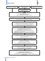
The procedure is straightforward: you just go over the three buttons "Location", "System" and "Results".
First click on "Location" button: you have to give a description of your pre-sizing project in order to identify
it after saving. The pre-sizing projects are simple files which don't allow for several variants.
Choose a location in the database. You can obtain the location details, or even create or import a new
location from Meteonorm 117 or US TMY data 119 , using the "open" button.
When necessary you can also define an Horizon
38
profile.
Click on "System" button. The pre-sizing procedure is then specific for each type of system:
Grid-connected system
Stand-alone system
Pumping system
17
21
19
.
Chapter 2 Licensing
18
,
,
3
Preliminary design
Grid System Presizing
Pre-sizing is a rough estimation of the PV system energy yield, based on a few very general parameters
and mainly dedicated to architects during an early evaluation of a site. You should not use this tool for the
study of a system.
The meteo input data are computed in monthly values (taking plane orientation and horizon into account)
and applies efficiency coefficients according to a PV technology and other considerations. These
coefficients may eventually be re-adjusted by an expert user for special conditions in the Hidden
parameters 173 . The expected precision could be around 10% or more.
More precise results will be obtained with the hourly simulation performed through the "Project Design"
option, including realistic available components and detailed system perturbations.
Especially the financial aspects are based on coarse hypothesis, which can widely vary from country to
country. These hypothetic financial parameters can be adjusted by the user by choosing "Edit costs" in the
economic results sheet.
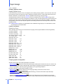
Grid-connected system preliminary design
After defining the "Location" 17 the "System" button displays a first screen where you should first define
the plane orientation (try dragging little red dots!).
NB: a little tool helps for the choice of the optimal orientation
choice when not optimal.
33
, or the amount of losses resulting of you
Then you have to choose if you want to size your system on the basis of:
- Active area of the collector field
- Nominal power of the system
- Annual energy yield.
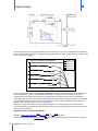
Pressing "Next" gives a second screen for defining system properties, especially from the architect point
of view:
- Module type: "standard" (give also the module power), "translucide custom" (with spaced cells, you
should define the filling ratio), or "not yet defined".
- Technology: will determine the default efficiency, that is the needed area for a given power.
- Mounting disposition: indicative, not used in calculations,
- Ventilation property: will slightly influence the efficiency due to module operating temperature.
Now you can open the "Results" which gives the Nominal Power, Area or Annual energy yields, as well as
some result graphs, table and economic evaluation 22 (to switch from one to the other please use speedbuttons left).
You can now play with the parameters and immediately see the results.
You can print a report, or store graphs and tables in the clipboard to export it to another software.
You can also save your project, and load another one for immediate comparisons.
Computation:
The evaluation of the available irradiance on the collector plane uses the Monthly Meteo 184 tool algorithms,
and the system energy output computations are done using constant efficiency and correction coefficients
according to the chosen system parameters.
The accuracy is of the order of 10 - 20% (worst case for façade installations).
If necessary the coefficients used for this tool may be modified in the Hidden parameters 173 .
Chapter 3 Preliminary design
18
3
Preliminary design
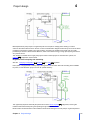
Stand-alone system presizing
Pre-sizing is a rough estimation of the PV system energy yield and user's needs satisfaction, based on a few very
general parameters. It is aimed to determine the size of the optimal PV array power and battery pack capacity
required to match the user's needs.
The input solar energy is computed in monthly values (taking plane orientation and horizon into account), and
requires only the monthly data provided by the "Sites" database.
Besides the Battery voltage – which is related to the overall system power and geographic extension (due to
distribution ohmic losses), the two basic user parameters are:
The desired system autonomy (in days), which determines the battery capacity,
The required LOL, giving the required PV array nominal power.
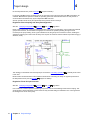
After sizing the PV system with this tool, it's real performances should be verified by performing a detailed hourly
simulation (option "Project design"), using real components and taking all system perturbations into account.
Stand-alone system preliminary design
See also: Sizing of a stand-alone PV system
20
: general considerations.
After defining the "Location" 17 the "System" button displays a first screen where you are asked to define the
plane orientation.
NB: the button "Show optimization" opens a little tool which shows the winter yield according to the plane
orientation. For stand-alone systems, the plane orientation should usually be optimized according to the
worst conditions, i.e; for winter irradiance.
Pressing "Next" gives a second screen for defining the user's needs 189 , from a domestic use point of view. You
have to specify every foreseen appliance, their consumption 56 and use conditions.
Now you can open the "Results" which asks for
- the required autonomy 188 in absence of sun - which determines the battery pack capacity,
- the required "Loss-of-Load probability" 191 (P LOL) ,
- the planned system voltage 20
These parameters lead to the determination of the array nominal power (i.e. the installed STC
according to the manufacturer specifications), and the battery pack capacity.
194
power
The first result graphs shows the potentially available solar energy, along with the user's needs.
The second one gives the average state of charge of the battery (low values could lead to a quicker deterioration
of the batteries), and PLOL monthly distribution.
The table holds all monthly values, including then needed back-up energy.
Finally the rough economic evaluation 22 gives an idea of the investment and energy price.
You can now play with the parameters and immediately see the results.
You can print a report, or store graphs and tables in the clipboard to export it to another software.
You can also save your project, and load another one for immediate comparisons.
Computation:
The evaluation of the available irradiance on the collector plane uses the Monthly Meteo 184 tool algorithms, which
calculate irradiation's monthly averages on the basis of instantaneous data for one day per month.
This is not sufficient to manage the storage balance evolution from day to day, and the effective use of solar
incident energy. Therefore the program generates a random sequence of 365 days, according to the algorithms
of Collares-Pereira, renormalised to the monthly sums, and calculates the daily battery balance for three intervals
in a day (morning, day and evening).
The accuracy is of the order of 10 - 20% (worst case for very tilted installations).
If necessary the general parameters (array overall efficiency, battery efficiency, battery low charge threshold) are
user-modifiable through the menu option "Preferences"/"Edit Hidden Parameter" 173 .
19
Chapter 3 Preliminary design
3
Preliminary design
Stand-alone system design
When sizing a PV stand-alone system, the basic constraints are the availability of solar energy during the year,
and the satisfaction of the user's needs. The problem to be solved is the optimisation of the size of the
photovoltaic generator and the storage capacity, subjected to criteria which may take on different weights
depending on the use:
-
Reliability of the supply, which is very important, for example in decentralised telecommunication
installations. But in a domestic installation, this may be overcome with a small back-up generator. This
reliability is measured as the "Loss of Load" Probability ("P LOL").
-
Investment and maintenance costs, which should take into consideration the cost of the PV generator, the
initial cost of the batteries, as well as that of their maintenance and replacement. The high price of the kWh
used necessitates a highly detailed study of the real user's needs, and the use of specific appliances that are
highly economical regarding to energy consumption.
-
Durability: the cost of the batteries is closely related to the quality of the batteries chosen, as well as their
longevity, which is itself dependent on the conditions of use (average state of charge, cycling, depth of
discharge, temperature).
It is therefore observed that the optimisation of a PV system is a complex problem with several criteria, which has
no ready-made solution. The preliminary design tool allows for "playing" with the main parameters, and rapidly
observe their effects on the system performance, to optimise the desired characteristics by successive
approximations.
But the accuracy of these monthly results is not guaranteed and the behaviour of the chosen system will have to
be verified by a complete simulation in hourly values, with real available components.
Battery Voltage Choice
Battery Voltage Choice
In a stand-alone PV system with direct coupling to the user (without inverter), the battery voltage determines the
distribution voltage. As now many DC appliances can be found as well in 24V as in 12V, this choice should be
made according to system and/or appliance power, as well as the extension of the planned distribution grid to
minimise the ohmic wiring losses.
This choice should be done from the early planning of an installation, since the existing appliance voltage usually
cannot be changed, and voltage translators will be expensive and not 100% efficient.
The rated distribution values could be chosen according to the following criteria (inverter supposed directly
connected on the battery pack):
12V: little systems for lighting and TV:
Appliance max power
Corresponding current
Inverter : about
< 300 W
25 A
< 1 kW
24V: medium size, with fridge and little appliances, or wiring extension to more than 10 m.
Appliance max power
< 1000
W
Corresponding current
Inverter : about
48V: special industrial or agricultural use
Appliance max power
Corresponding current
Inverter : about
42 A
< 5 kW
< 3 kW
62 A
< 15 kW
Higher powers require either high DC voltages (special appliances) or AC feeding
through inverter.
Chapter 3 Preliminary design
20
3
Preliminary design
Pumping system preliminary design
See also: Sizing of a pumping PV system
After defining the "Location"
17
66
: general considerations.
the "System" button displays a dialog where you are asked to define:
On the right panel: the plane orientation.
NB: the button "Show optimization" opens a little tool which shows the winter yield according to the plane
orientation. For stand-alone or pumping systems, the plane orientation should usually be optimized
according to the worst conditions, i.e. for winter irradiance.
On the left panel:
- The Water needs (in yearly, seasonal or monthly values).
-
The nominal head at which it should be pumped (level difference between water outlet and source surface).
The diameter and length of pipes (optional, for eventual friction losses).
A pump technology (centrifugal for rather low heads, positive displacement for high heads).
An array-pump coupling strategy, which strongly affects the system performances.
Now you can open the "Results" which asks for choosing:
- either the tank volume, or the autonomy of the system in days. These parameters are coupled, according to the
daily needs of water.
- the "Loss of Load" probability (P LOL), i.e. the time fraction during which the operator will accept that the needs
are not met (tank empty).
These parameters lead to the determination of the array nominal power (i.e. the installed STC 194 power
according to the manufacturer specifications), and the pump nominal power required. These are very rough
estimations, as the pumping system performances are strongly dependent on the pump technology, head,
flowrate, as well as the electrical matching between pump and PV array.
The first result graph shows the potentially available solar energy, along with the user's water and energy needs.
The second one (available by the speed buttons on the left) gives the average filling state of the tank, and the
missing water (P LOL) monthly distribution.
The table holds all monthly values, including an eventual required back-up energy.
Finally the rough economic evaluation 22 gives an idea of the investment and water price.
You can now play with the parameters and immediately see the results.
You can print a report, or store graphs and tables in the clipboard to export it to another software.
You can also save your project, and load another one for immediate comparisons.
Computation:
PVsyst performs a very simplified simulation, which runs over one year in daily values.
The evaluation of the available irradiance on the collector plane uses the Monthly Meteo 184 tool algorithms, which
calculate irradiation's monthly averages on the basis of instantaneous data for one day per month.
This is not sufficient to manage the water storage balance evolution from day to day, and the effective use of solar
incident energy. Therefore the program generates a random sequence of 365 days, according to the algorithms
of Collares-Pereira, renormalised to the monthly sums, for calculating the daily balance from day to day, and the
PLOL.
This simulation is repeated with different array and pump size arrangements, until matching the input
requirements (namely the desired PLOL). The program is able to propose:
- The pump(s) size (power),
- The PV array nominal power
- A rough estimation of the investment cost and the cost of water pumped.
If necessary the pre-defined parameters used (array, system matching and pump efficiency, etc.) are usermodifiable through the menu option "Preferences"/"Edit Hidden Parameter" 173 .
Of course, this early layout proposition should be asserted by a detailed simulation, using real commercially
available components, and taking all system features into account in an hourly modeling.
21
Chapter 3 Preliminary design
3
Preliminary design
Preliminary design: economic evaluation
Costs are given as specific costs for modules, other components, mounting, financial costs , taxes and so on.
Modules and inverter costs are dependent on the quantities.
Mounting and maintenance costs follow an exponential rule, referred to a 5 kWp system, with an exponential
coefficient of 0.8:
Cost = (Pnom / 5 kWp)**0.8 * Basecost (for 5kWp).
These hypothetic default financial parameters can be adjusted by the user by choosing "Edit costs" in the
economic results sheet.
Please be aware that at this pre-design stage costs are based on very coarse hypothesis. They can widely vary
from country to country, from time to time or from user to user (what costs are included here? customer or retailer
costs? which interventions on the building? designer fees? taxes? … etc).
The economic evaluation 102 at the detailed simulation stage will offer a flexible and more precise tool for
evaluating real costs according to the specific user's criteria.
This part is aiming to perform a thorough PV-system design and performance analysis using detailed hourly
simulations.
These are organised in the framework of a Project, which essentially holds the geographical situation and
meteorological hourly data. Optimisations and parameter analysis can be performed through different simulation
runs, called variants.
Procedure:
NB: You have a step-by-step tutorial
24
for elaborating your first project.
After choosing "Project Design" and the system type in the main window, the procedure is the following:
-
First define the Project
through the "File" menu.
-
For one Project (including basically Geographic Location and Meteo, with eventual Albedo data), you can
construct different system variants (as much as needed).
-
For each variant, define the plane orientation
-
Define the System
-
The program verifies the consistency of all parameters, and produces "Warnings" as Orange (acceptable for
simulation) or Red (preventing simulation) LED's.
-
When available (all parameters properly defined, that is only Green or Orange LED's), press the "Simulation
88 " button. Red buttons or warnings indicate bad definitions which prevent the simulation.
-
When the simulation is completed, you will enter the "Results
"Report" document.
-
After simulation, each variant may be saved for further comparisons (please use "Save as" for not overwriting
your previous variants). You are advised to define a significant description for each variant, in order to easily
retrieve them in the list and to obtain a suited title in your final report.
29
28
through the "Project/Variant" button. You can also retrieve an existing project
30
.
properties.
92
" dialog, and consult the main results on the
For a given project, you are advised to first construct a rough variant keeping all parameters to their proposed
default values.
In a second step, you can define the required refinements:
-
In the "System" definition panel, you can modify the "Detailed losses"
resistance, module quality, mismatch, soiling, IAM).
-
eventually define a Horizon profile
-
Near shadings 37 , that is partial shadings of near objects, which require a rather complex CAO 3D
construction of the PV-field environment.
38
82
(temperature parameters, wiring
(far shadings),
The next table shows an outline of the project's organization and simulation process.
Chapter 3 Preliminary design
22
4
Project design
Hourly meteorological data
(Reference Year, TMY, Satellight)
Monthly meteorological data
(Sites database)
Hourly meteo measurements
(Custom, horiz. or in coll. plane)
Generation of
synthetic hourly values
Project
Specification of the site (geographic coordinates)
Hourly meteorological data
Eventually Meteorological corrections (Albedo, Altitude, etc)
Simulation variant
(Many simulation variants may be defined for a given project)
Incident irradiance in the collector plane:
Transposition from horizontal values to the collector plane
(fixed plane, tracking 1 or 2 axes, seasonal adjusment, heterogeneous fields)
If "infinite" sheds or sun-shields: mutual shadings calculation
Far shadings (Horizon definition)
The far shadings affect the whole field at a time
Near shadings (partial shadings on the field)
Shading of near objects require a detailed 3D description of the system
Shading factor for beam component: "linear" or according to modules
Shading factor for diffuse: spherical integral of the "linear" shading factor
User's load
Necessary for Stand-alone and Pumping systems sizing
(Optional for Grid-connected)
Constant, monthly or daily profiles, or custom file data
PV array
Choice of PV modules (library)
Number and interconnections of modules
Specification of Losses (In a second step) :
Module quality, Mismatch, Thermal, Wiring resistance, Incidence angle (IAM)
System
Grid-connected, Stand-alone, Pumping, DC-Grid
Choice of the components and configuration
Simulation of the system (by hourly steps)
Results for a simulation version:
Complete engineer report - Economical evaluation
Customised Tables, monthly, daily and hourly graphs. - Detailed Loss diagram
ASCII export file.
23
Chapter 4 Project design
4
Project design
Project design: tutorial
Return to the Project design
22
definitions
For your introduction to the elaboration of a project in PVsyst, we will construct step-by-step a full project, located
at Marseille (France).
The main stages, which you are advised to follow for each of your future projects, are:
- Define the project, which holds mainly the geographic location and the meteo file used.
- Define a first system configuration with the minimal parameter set, let PVsyst fix other parameters to default
(reasonable) values). Simulate and save this variant.
- Define successive variants by adding progressively perturbations to this first system. I.e. far shadings, near
shadings, define specific loss parameters, etc.
You can save each variant for further comparisons.
Definition of the Project
The project is the central object (file with *.PRJ extension) for which you will construct different variants of your
system (files with the same name, and extensions *.VC0, *.VC1, etc for "calculation version").
- In the main page of PVsyst, choose "Project Design" / "Grid connected".
- In the next window, choose "Project", and then button "New project".
- Define the "Project's name". This will appear in the Project's list choices and on the final report. The other
definitions in this dialog are only for memory, they are not used elsewhere in the software. You can put for
example "Tutorial at Marseille".
- Click the button "Site an Meteo".
- Choose a site in the "sites" database (contains geographic location and monthly meteo data). We will chose "
Marseille".
NB: If you want to define your own site, which is not in the database, it is preferable to define it first in the
database, using "Tools" / "Geographical Location)".
- This automatically produces a synthetic hourly data file named "Marseille_Syn.MET".
NB: At this stage you can choose another meteo file in the (*.MET) available data if desired.
- Click the "Alb edo" button. Usually you will never modify the albedo factor. The value of 0.2 is a standard adopted
by everybody. Nevertheless if you are for example in mountain weather with some snow, you can define one or
two months with 0.8.
- Click "OK". You will be prompted to save the project file. The description had already defined previously. Give a
synthetic identifier for the file name, without special characters like accents. All the files referred to this project
will have this name. You can define for example "Marseille_Tutorial".
- Save the project.
Creating your first variant for this project
- In the Project's dialog, button "Back (Calculation)".
In this window: a red button means parameters to be defined, or not acceptable.
An orange button means acceptable, but not ideal parameters.
A green lighted button means: Parameters defined, correct.
A green out button, that this topic is not defined for this version.
The "Simulation" will be enabled only when no button is red.
- Click "Orientation" button: choose "Fixed tilted plane", Tilt = 25°, Azimuth = 20° (toward east).
NB: When defining the Orientation, you have a tool "Show optimization" for situating your choice by respect to
optimum (regarding the transposition factor). The optimum is different for grid-connected systems
(optimization on the whole year) or stand-alone/pumping systems (optimization on the more critical
period).
- Click "System" button: definition of the PV system. Will open the system definition dialog.
- In the "Presizing Help" group, define "Availab le Area" = 125 m².
- Choose a PV module. The list will show "All modules", or your "Favorites", or other categories according to
Chapter 4 Project design
24
Project design
4
availability. You can sort them by manufacturers, and then choose for example a module of Photowatt, say the
PW1000/110W.
- Choose an inverter. The comment in the "Design the array" will propose a suited power for the inverter(s). In this
project we will choose 3 inverters of 4.2 kW, for example Diehl, Platinum 4800 TL.
NB: the button "Show sizing" will open a window where all the sizing constraints are apparent. Here we see
that the maximum voltage of the PV module (here 600V) is a strong limit for this system, far below the
Inverter's VmaxAbs (880 V) or even Vmppmin (710V).
- Now the warning panel doesn't show any warning (in orange: not optimal, in red: would prevent the simulation).
Only by defining the size of the system and the components, PVsyst has proposed an acceptable design for your
PV system. You can click "OK".
Executing the simulation
- You can now click the "Simulation" button, which is now activated as there are no red buttons.
- Give a significant description of this variant (for example "First simulation"),
- Press the "Simulation" button, and at the end "OK".
- Click button "Results", and then "Report".
Results
This shows the report of your first simulation, which has now 3 pages:
- First page: all the parameters for this simulation,
- Second page: a reminder of the parameters, the main results, graphics of normalised values 96 , and table of
monthly values,
- Third page: an arrow loss diagram 93 , showing an energetic balance and all losses along the system. This is
a powerful indicator of the quality of your system, and will immediately indicate the big sizing errors if any.
Saving your simulation
You should now "Save" this first variant for further comparisons. This will be saved as " Marseille_Tutorial.VC0".
Be careful: use "Save As" for avoiding overwriting your previous variants if any.
For opening previous simulations of the project, click "Load" just above.
Adding further particularities of your project
After this first "standard" simulation, you can progressively add the specificities of your particular project. You are
advised to perform a new simulation at each step in order to check its effect and pertinence - especially by
analysing the "Loss diagram".
Far shadings, Horizon profile
This is only suited for shading objects sufficiently far from your PV system, so that the shadings may be
considered global on your array. The distance of the shading object should be, say, over about 10 times the PV
system size. The Horizon Profile is defined as a curve, set of (Height, Azimuth) points .
The Far Shadings operate in an ON/OFF mode: i.e. at a given time, the sun is or is not present on the field. When
the sun is behind the horizon the beam component becomes null. But the diffuse component, supposed isotropic
- coming from all points of the sky vault seen by the collectors with an identical intensity - is not much affected.
Clicking the "Horizon" button will open a graph of the sun paths at your location.
25
Chapter 4 Project design
Project design
4
Defining horizon line by hand:
The horizon (Height, Azimuth) values may be recorded on-site using a compass and a clinometre (measuring the
height angles) or a land surveyor instrument.
You can move any red point by dragging it with the mouse, or define accurately its values in Edit boxes.
For creating a new point right-click anywhere. For deleting a point right-click on this point.
You can of course save this horizon as a file fur further use in others projects in PVsyst.
Importing Horizon from Solmetric "SunEye" instrument
The "SunEye" records the horizon line using a fisheye camera, and provides results as files. You should choose
the "Ob structionElevation.csv" file. Don't use the "Sky0x_PVsyst.hor" file, which was elaborated by Solmetrics for
the old versions 4.xx of PVsyst.
NB: You should correct the data if near objects are represented in the record.
Importing Horizon from the "Carnaval" software
Carnaval is a georeferred software (including altimetric data) able to establish an horizon line for any place given
by its exact geographical coordinates - Latitude and Longitude - in France and neighbours. You should not use
the near objects option in this software for establishing far shadings PVsyst masks.
Carnaval produces a file named "YourProject.masque.txt". Please rename this file by removing the ".masque"
characters as PVsyst doesn't accpt file names with 2 points.
Importing Horizon from the "Horiz'ON" software
The "Camera Master" tool is a specialized support for your Photo Camera, which allows to take several
photographies with an horizontal reference (every 20° in azimuth). The software "Horiz'ON" gathers these photos
as a single panorama on which you can draw the horizon line by mouse. This produces a file directly readable in
PVsyst.
NB: when established using a georeferred grid (like Carnaval or Meteonorm), the exact location should be
carefully defined. This may be determined using GoogleEarth or a GPS. Please remind that a degree in latitude is
111 km, a minute is 1850 m and a second is 31m.
Near shadings, 3D construction
If you have near shading masks, you should construct your PV installation and the neighbours as a 3D scene (
see the dedicated tutorial 49 ). The previous instruments (including SunEye) cannot help for this construction,
which should be realized using architect's planes or equivalent, including heights indications.
You will performe the simulation with linear shadings (irradiance deficit, lower estimation of the shading effect),
and then "according to module strings" (upper bound of the electrical effect, higher estimation of the shading
losses).
Finally, for the definitive report to be transmitted to your customer, you can choose an intermediate value for the
electrical effect, taking the by-pass diode recovery into account. For this you have to choose an intermediate
fraction of electrical effect, which will depend on your system geometry. But we don’t have well-established value
Chapter 4 Project design
26
Project design
4
to propose at the moment (60 to 80% ??? - Higher for regular shadings like shed mutual shadings !).
NB: The near shading loss doesn't cumulate with the far shadings: when the sun is behind the horizon, the beam
component is null, and therefore there is no near shading contribution.
Final layout of your system
There is in principle no relation in the program between the definition of the system, and the definition of your 3D
scene. Except that at the end of the process the program will check the compatibility of these different parts.
Namely it will require that the plane orientations are identical, and that you have defined a sufficient sensitive area
in the 3D scene for installing the PV modules defined in your system.
But PVsyst doesn't check the real physical (geometrical) compatibility. In a second step, you should check the
arrangement of your modules, and eventually modify the system definition (number of modules in series and
parallel) in order to build a realistic installation. PVsyst doesn't offer specific tool for this try-and-error process in
the present state.
Array losses
Finally there are several parameters which are fixed by PVsyst as reasonable default values for your early
simulations, but that you should modify according to the specificities of your system. These are available in the
"System" definition dialog, button "Detailed losses".
Thermal Losses
The thermal behaviour of the array is computed at each simulation step, by a thermal balance 85 . This
establishes the instantaneous operating temperature, to be used by the PV modules modelling.
The thermal balance involves the "Heat loss factor" U = Uc + Uv · WindSpeed [W/m²·K]. In practice we advise not
to use the wind dependency, as the wind speed is usually not well defined in the meteo data, and the Uv is not
well known. Therefore we put Uv = 0 and include an average wind effect in the constant term.
According to our own measurements on several systems, PVsyst proposes:
- Uc = 29 W/m²K for complete free air circulation around the collectors ("nude" collectors).
- Uc = 15 W/m²K for integration (back insulated), as only one surface participates to the convection/radiation
cooling.
- We don't have well-established values for intermediate situations with back air circulation. Our measurement on
quasi-horizontal modules on a steel roof, 8 cm spacing and not jointive collectors, gave 18 W/m²K;
NB: up to the version 5.1, the default value was 29 W/m² (free standing). From this version the default is set to 20
W/m² as more and more installations are integrated.
The thermal loss effect is visible on the array loss diagram.
Wiring Losses
The wiring ohmic resistance induces losses 84 ( R · I² ) between the power available from the modules and that
at the terminals of the array. These losses can be characterised by just one parameter R defined for the global
array.
The program proposes a default global wiring loss fraction of 1.5% by respect to the STC running conditions. But
you have a specific tool 84 for establishing and optimizing the ohmic losses (press "Detailed Calculation"
button). This tool asks for the average length of wires for the string loops, and between the intermediate junction
boxes and the inverter, and helps the determination of the wire sections.
NB: remember that the wiring loss behaves as the square of the current. Therefore operating at half power (500
W/m²) will lead to only a quarter of the relative loss. The effective loss during a given period will be given as a
simulation result and shown on the loss diagram. It is usually of the order of one half to 60% of the above
specified relative loss when operation at MPP.
This part also includes the definition of eventual losses between the output of the inverter and the injection point
(energy counter). You have just to define the distance and the loss will also appear in the loss diagram.
Module quality loss
The aim of this parameter is to reflect the confidence that you put in the matching of your real module set
performance, by respect to the manufacturer's specification. The default PVsyst value is half the lower tolerance of
the modules.
The result in the "Array loss diagram" is not exactly the specified value, at this is referenced to the STC when in
the diagram value it is by respect to the previous energy.
27
Chapter 4 Project design
4
Project design
Mismatch loss
Losses due to "mismatch" are related to the fact that the real modules in the array do not rigorously present the
same I/V characteristics. Remember that in a string the worst module drives the string's current.
The button "Detailed computation" helps the understanding of this phenomenon, and gives indications on the
loss parameter to be set for the simulation, according to your hypothesis on your effective module set.
This parameter acts as a constant loss during the simulation. It is lower for thin film modules. It could be about
null when sorting the modules according to their real performance (flash-test results provided by the
manufacturer).
NB: There is probably a correlation between these 2 last parameters. The Module quality loss is rather related to
the average of the module's distribution, when the mismatch refers to its width.
Soiling loss
To our experience, the soiling effect is about negligible in middle-climate residential situations.
It may become significant is some industrial environments (for example near railway lines), or in desert climates.
The monthly definition allows for taking periodical cleaning or rains into account.
This parameter may also be used for describing a snow effect (for example put 50% in winter month with 15 days
coverage).
IAM loss
The incidence loss (reflexions due to the fresnel's laws) is sufficiently well defined by parametrization proposes
by the "Ashrae" (US standards office). You will in principle never modify this parameter.
NB: Assuming an isotropic diffuse, the IAM factor on the diffuse part is computed by an integral over all spaces
directions, which include important low-incidence contributions.
Project definition
When creating a project you have to define:
-
The project name, which will identify the project in the file list in your data library.
-
The PV system customer address (facultative, not used elsewhere in the software),
-
The geographical location 110 ,
-
The hourly meteo file 109 in internal PVSYST format (*.MET files).
NB: These are defined in the Project Situation and Meteo
and meteo file may be of different kinds.
-
29
dialog. The relations between Geographical site
Finally the "Next" button leads to the definition of the albedo 187 characteristics of the project site.
The project parameters are stored in a file with the extension .PRJ. All variants will have the same with
extensions .VC0, .VC1, etc.
Site and Meteo data in the Project
The project is located at a geographical Site 110 . Sites are described in *.SIT files, with geographical coordinates
and meteo in Monthly values.
The detailed simulation process requires the following meteorological hourly data:
- Horizontal Global Irradiance
- Horizontal Diffuse Irradiance (optional, may be constructed by a model),
- Ambiant Temperature,
- Wind velocity (optional, for module temperature calculation).
These data are stored in meteo files 109 , written with the internal PVSYST format ( *.MET files).
When creating a project you will usually first choose a Site in the database;
By default, if no matching meteo file (same name as the project site) is available in the library, a Synthetic Hourly
Data 186 file will be automatically generated from the monthly meteo data defined for the Project site.
Chapter 4 Project design
28
4
Project design
But you can also choose an existing meteo hourly file in the library (for example, 22 Design Reference Years for
Switzerland in the PVSYST library).
You can also obtain Hourly Meteo files in several ways, all available in the "Tools" part of the software:
-
Import an synthetic hourly meteo file from the Meteonorm 117 software,
-
For the US, import a US TMY2 119 file (Typical Meteorological Year) available from the web (free),
-
For the whole Europe, import measured data from the Satellight 120 project (free).
-
Convert any custom meteo ASCII file 126 (your own measurements, or Design Reference Year of other
sources, etc.), using the PVSYST special converting tool.
Project Site and Meteo
When creating a project 28 the Geographical Site and Meteo may be defined in several ways.
Please remember that a geographic site is attached to the project (your project's location) and another
geographical site is defined within the hourly meteo file. These sites are not necessary identical. When different,
the climatic distance will be mentioned; this should not exceed some dozens of km.
Standard procedure
- Choose a geographical site in the database.
- If a corresponding meteo file (same site name) is available in the Meteo database, this will be automatically
selected.
- Otherwise a synthetic hourly file will be automatically created according to the monthly data of your site.
Standard procedure with customised site name
- Choose the nearest available geographical site in the database.
- Modify the site name (which will appear on the final reports for the customer) by opening the site. This will of
course keep the meteo monthly values of the original site.
- You can also modify (not too much, say < 1-2°) the coordinates (Latitude/Longitude). These values will be taken
as basis for constructing the eventual synthetic meteo file, and in the solar geometry (namely transpositions)
within the project.
- If a corresponding meteo file (same site name) is available in the Meteo database, this will be automatically
selected.
- Otherwise a synthetic hourly file will be automatically created according to the monthly data of your site.
Starting from a meteo data file
- Choose the desired Meteo file in the database.
- Copy Meteo Site => Project Site.
- You may change the site name and coordinates if desired.
In this dialog:
- The opportunity of copying the site from a meteo file to the project, or inversely to generate a synthetic hourly file
from the Project's site (normally performed automatically), are available as soon as the location coordinates are
different.
- If you need other meteo data , please define them in the database, using "Tools" / "Geographical site" or "Import
meteo data".
- When different sites, the climatic distance 189 between the sites is shown.
- If the altitudes are very different, altitude corrections
project's site altitude.
188
may be applied to your Meteo data for matching the
System definition
The system definitions are primary aimed to define all the PV_system components necessary to fulfil the user's
29
Chapter 4 Project design
4
Project design
wishes.
In a second step, this part gives the possibility of modifying the PV-array specific loss parameters (thermal, wiring
resistance, module quality, mismatch, IAM) (button "Array losses"). All these parameters are initialised at typical
default values, so that first calculations give likely "average" results.
In stand-alone systems the user's needs definition are absolutely necessary. They closely condition the system
design.
For grid systems, these can be defined afterwards in order to obtain the user self-consumed energy part and the
energy reinjected into the grid.
In DC-grid systems, especially for public transport, the instantaneous need could be lower than the produced
energy at some instants, so that there will be some unused energy.
Parameter definitions are of course different according to system types:
Grid-connected systems 57 ,
Stand-alone systems 63 ,
Pumping systems 65 .
DC-grid connected systems 64 ,
Plane orientation
PVSYST supports simulations with many plane orientation modes:
-
Fixed tilted plane: You have just to define the Plane tilt 193 and azimuth 193 .
-
Seasonal tilt adjustment: the plane tilt may be adjusted with two values, for winter and summer chosen
months.
-
Tracking, two axes: the limit mechanical angles of the tracking device (in tilt and azimuth) should be defined,
and are taken into account during the simulation.
-
Tracking, two axis with frame: the collectors are fixed and rotating within a frame, itself rotating. Two
configurations are available: a frame with North-South axis (and collectors with tracking tilt) or a frame with
East-West axis (and collectors tracking according to the sun azimuth).
-
Tracking, tilted axis: the axis's tilt and azimuth should be defined (the axis azimuth will usually be around 0, i.
e. near the south in northern hemisphere). The rotation angle is called Phi (value 0 when plane azimuth =
axis azimuth), with the same sign conventions as for plane azimuth 193 . Limits on the Phi stroke are required.
-
Tracking, horizontal axis E-W: the orientation axis is defined as the normal to the horizontal axis. Stroke limits
should be defined (here Phi = plane tilt), from lower limit (minimum -90° = vertical north) to upper limit
(maximum 90° = vertical south). This configuration is indeed not suited for PV systems.
-
Tracking, horizontal axis N-S: this is the usual configuration of horizontal axis tracking systems. You should
use the "Tilted axis" option, with axis tilt = 0°.
-
Tracking, vertical axis: the collector is kept at a fixed tilt, but rotating according to the sun azimuth. This
configuration may be used with "dish" arrangements, when a big rotating support holds several rows of
modules; this particular case is made possible as the rotating axis of one row may displaced by respect to the
collector.
-
Tracking sun-shields: which may yield solutions to the difficult optimisation between sun protection and PV
production. For full efficiency this should involve a Backtracking 45 control strategy.
-
Double orientation: allows to define two collector planes with different orientations. You should define the
fraction of the field allocated to each orientation. Warning: the PV modules of a same string should all have the
same orientation. The electrical behaviour of modules connected in series and having different orientations is
very complex and not functionally optimal (see the specific related tool) and is not supported in the simulation
process.
-
Unlimited sheds: 31 To be used when the sheds are very long by respect to their width. If the sheds are too
short as one cannot neglect the edge effects, you should define sheds in the "Near shadings" CAO option
instead.
-
Unlimited sun-shields:
33
Chapter 4 Project design
Same remarks as for sheds. The optimization of electrical yield of sun-shield
30
Project design
4
systems is very difficult, and only suited for south façades.
Limitations
The tracking strategy in only computed using the solar geometry (so-called "astronomical" algorithms). A
simulation using a strategy with irradiance optimization on the collectors is much more complex to implement,
and is not yet available in PVsyst.
Please note that the near shading calculations cannot be applied to Seasonal Tilt adjustment. For double
orientation (heterogeneous fields), the shading factor is computed once for both fields at a time, so that it
becomes not well applicable (induces errors) when the difference in orientation is too big.
For sheds, please carefully see the special combination of "Orientation" option and "Near shadings" treatement
43
Also be aware that with tracking planes, the mutual shadings of several neighbour tracking units can become very
important at extreme angles (see the "shed" optimization tool 31 with very tilted collector plane!). The collector's
spacing should usually be very large, so that the horizontal space use is rather low. Also Backtracking 45 control
strategy may help optimizing the electrical yield.
Heterogeneous Fields
It is commonly admitted that in a PV field, all the collectors should be perfectly identical and have the same
orientation. This tool allows the phenomenological analysis of the effect of not observing this rule. It shows the
characteristic of two fields, connected in parallel, which can be different in orientation and collector's number.
A rigorous energy analysis is also possible in the framework of the simulation. In "Project design", and
"Orientation" parameters, choose the Field type: "Doub le orientation".
When connecting together the outputs of 2 different arrays, the resultant characteristic will depend on incident
irradiances on each of the sub-fields. It is therefore necessary to introduce a model for the irradiance, in such a
way as to be able to evaluate simultaneous irradiances under realistic conditions along the day. The tool uses a
clear day profile, but with the possibility of modulating the global amplitude and the rate of diffuse irradiation, to
approach the meteorological conditions of any day. The temperature of the modules is calculated according to the
respective irradiances. The user may use the scroll bar to modify the time-of day, in order to evaluate the dynamic
behaviour during the day when the orientations are different.
The graph shows the respective I/V characteristics of each sub-field, and their resultant (current sum) when
connected in parallel. The comment gives the nominal MPP value of each array, as well as their common value
and the relative loss when connected in parallel.
One can see that when the array voltages are comparable the power loss is usually low, even for very different
currents (different orientations along the day, or different parallel strings). In this case the performances of each
array are simply added together.
But for different voltages the resultant characteristic shows two distinct maxima, with a serious loss of power.
This could also induce the MPP tracking device into error, as it may "choose" the secondary maximum.
When the arrays are expected to operate under different voltages (heterogeneous arrays, but also by partial
shading effects), it is also very important to connect blocking diodes in each string. The dotted line shows the
resulting behaviour if these diodes are omitted: the production of the higher array may flow into the lower one,
inducing a feeding power into the "overvoltage" region.
Sheds mutual shadings
PVSYST offers a special tool for viewing and optimising the shed mounting (and also sun-shields). This is
implemented in several places in the software:
31
-
In "Tools" / "Tab les and Graphs of Solar parameters", you can define the geometry, optimise it with the mouse,
and view the mutual shading effects of your choice on an Height/azimuth diagram.
-
In "Tools" / "Monthly Meteo Computations": you can moreover have a quick meteo calculation for your site, and
immediately estimate the irradiation losses over the year.
-
During the definition of the project's parameters, the "Orientation" choice offers the opportunity of defining
sheds or sun-shields. This will of course take the corresponding mutual shadings into account during the
simulation process (on beam as well as diffuse component).
Chapter 4 Project design
4
Project design
With these tools, the mutual shading of sheds (or sun-shields) is performed using a simple geometrical
computation, which gives the mutual shading fraction as a function of the Transverse Incidence Angle 194 or
"Profile angle" in the shed orientation.
-
This calculation is performed assuming sheds of "infinite" length (that is, it doesn't take the edge effects into
account).
-
The calculation may be performed for irradiance, i.e. the shading factor is the shaded area fraction of the full
array (depends only on the pitch and tilt angle). This also slightly depends on the number of sheds as the first
one is not shaded. This is what we call the "linear" shading.
-
You can also estimate the electrical effect of these shadings. Remember that the current of the whole string
(as seen from the inverter input) is limited to the current of the weakest cell, i.e. the shaded one. Therefore we
suppose that the production of the bottom string becomes null (regarding beam component) if the bottom row
of cells is fully shaded, and proportional to the shaded fraction of the cells otherwise. This is what we call
shading "according to module strings" in the near shadings.
Therefore this calculation requires the specification of the number of strings in the transverse dimension of
the shed, as well as the size of one cell. Please note that with thin film modules with "long" cells of around 10
mm width, the cells should be placed in the transverse dimension of the shed, so that only a little part of each
cell is shaded at a time.
The three parts of the shed tool: geometrical design, shading graph and yearly yield graph, are meant for a
better understanding when optimising 32 a shed layout.
Please carefully see the limitations when using sheds with near shading scenes
43
.
Shed optimization
Shadings on Beam and Diffuse
First of all, when optimising sheds, one should keep in mind that the shading losses are of two kinds:
- The shadings which we usually visualize, are applied on the beam component. They apply especially on some
periods of the day or the year, and often when the sun is not very "high" on the plane surface, therefore affecting
hours of rather low production (there can be an exception with mutual shading of sheds, reinforced by the
"electrical" effect of cell partial shadings).
- The shading on the diffuse component, which applies permanently with the same value when assuming an
isotropic diffuse distribution. This shading factor is related to the part of heavens which is "seen" by the
collectors. Remember that in central Europe climates, the Diffuse fraction is of the order of 50% of the total
incident irradiation !
In the shed disposition, the diffuse effect is particularly important as the heavens vault view is limited in front by
the previous shed (affecting rather high incidence angles) and to the rear side by the plane itself. Due to its
permanent effect, this is often the main part of the losses.
This situation is even much more sensitive with sun-shields.
General features and optimisation of sheds
With shed disposition, we should be aware that:
- The area occupation is strongly depending on the collector tilt. For acceptable shadings, the "Limit shading"
profile angle 193 should be kept below about 18° to 20°. With 30° collector tilt, this implies that you can only
install a collector area limited to 45% of the total available area.
- The mutual shading effect is also strongly dependent on the shed orientation: when not south, the morning or
evening performances are much more affected.
The software offers two complementary tools for well understanding these situations:
- The beam shading graph, which shows the periods which are affected by the shadings. One can notice that with
south orientation, the effects are rather limited to summer morning and evening. But as soon as you change the
azimuth, the shading losses increase rapidly, and arise especially in regions where the incidence angles are
high.
- The yearly yield graph shows the relative gain (by respect of the horizontal layout), as a function of the module tilt.
This factor is based on the yearly global useful irradiation (beam and diffuse) falling onto the collectors. The
Chapter 4 Project design
32
Project design
4
curves show the pure transposition yield (as if there were one only plane) and the curve with mutual shadings,
either "linear" and for electrical losses.
This graph can be drawn with two options:
- Either keeping the Incidence limit angle constant. In this case we see that the collection/ground ratio is very
sensitive to the plane tilt.
- Or keeping the Shed spacing (i.e. a chosen collection/ground ratio) constant.
In both cases, we see that the optimal tilt of sheds is lower than for a single plane. This is still more evident with
non-south azimuths.
From these tools we can observe that:
With shed installations, choosing a rather low tilt is often a very good solution, which leads to acceptable losses
of some few percent by respect to the optimum, with the following advantages:
- The installable power is much greater on a given ground area.
- The array orientation does no more affect the performances: you can install the sheds according to the building
geometry, special "south-facing" arrangements are no more useful.
- Module supports become more simple, cheaper and lighter, with less wind sensitivity.
- Architectural impact can be much more acceptable.
Nevertheless, the minimum tilt should be kept at some few degrees (2-3°) for module cleaning by the rain.
Moreover, frameless laminates should be used in order to avoid dirt and mosses accumulations on the bottom
side.
Sun Shields mutual shadings
In the "Orientation" option and for near shadings, sun-shields are treated in a similar way as sheds (see Shed
Mutual Shadings 31 discussion).
Nevertheless, the user should be aware of two phenomena:
-
With sun-shields, the accepted part of the diffuse irradiation is very limited: on one hand, there is at most only
one half because of the rear wall, and on the other hand the upper sun-shield also cuts an important fraction
of the remaining diffuse component. In regions with a high diffuse fraction (above 45° latitude, it is usually
more than 50%), this gives a very significant loss.
-
Please be very careful with orientations not exactly facing the south (or north in southern hemisphere). You
can use the special tool "Shading graph" to visualise this dramatic effects.
For simulations, if you define near shadings in the "Orientation" parameters and you want to define other near
shadings, please consider the collector plane in the Near shading scene as a vertical plane on the wall.
Orientation optimisation tool
When choosing the (fixed) plane orientation, an information panel indicates the corresponding Transposition
Factor, the difference (loss) by respect to the optimum orientation, and the available irradiation on this tilted plane.
Clicking the "Show optimization" button, you can see a graph of the Transposition Factor as a function of the
plane tilt and azimuth. These graphs also indicate your actual choice by a violet dot on the curves, showing at
once where you are positioned by respect to the optimum.
The optimisation of the orientation depends on the planned use for the PV energy.
-
For grid-connected systems, the energy is usually sold at a constant price all over the year. The relevant
optimum is then to maximize the yearly energy.
-
For stand-alone systems, the relevant solar yield for sizing the system is usually the winter months.
-
For pumping systems, there is no general rule, depending on the final use of the water pumped: household
(all over the year) or irrigation (some specific seasons, probably summer).
Therefore this tool gives the opportunity of choosing the optimizing period: Year, Winter or Summer (this option is
fixed according to the system type in the presizing part).
NB: This tool makes use of the Monthly Meteo calculations 184 , which perform quick transpositions from the
Monthly Meteo values. The whole calculation for the curves is performed for several situations, in both
directions from the point you have chosen (tilts at fixed azimuth, and azimuths at fixed tilt).
33
Chapter 4 Project design
4
Project design
Concentrating systems
Systems involving concentrating devices are not treated in whole generality in PVsyst. Some specific
features have been implemented from version 4.2, for evaluating especially high-concentrating systems. But
their accuracy is not quite established.
The general study of concentration systems involves a detailed description of the irradiance distribution,
which cannot be available using the present treatment of the Meteo, nor the limited information included in
the meteo database (site database).
Namely high concentrating performances require a good knowledge of the beam component. Then accurate
models for achieving this evaluation would involve parameter like turbidity, water and aerosol contents of the
atmosphere, which are not defined in our database.
As an example, the eruption of the Mt. Pinatubo in 1991, had little effects on the global irradiance (less
than 2%) but induced a very high loss of beam component: the pure direct was scattered by aerosols,
resulting in a strong halo around the sun, up to 30% during almost 2 years. This had dramatic
consequences on the productivity of the high concentration thermal plants all around the earth [Molineaux
1996]
In PVsyst, the simulation of concentrating systems has to deal with 2 aspects:
Acceptance of the Diffuse component
The higher the concentration, the lower the acceptance angle, which implies a limited acceptance of the
diffuse component.
The maximum achievable Concentration Ratio CR is related to the acceptance half-angle
as:
CRmax (1axis) = 1 / sin
CRmax (2axis) = 1 / sin²
(Kreith and Kreidler, 1978, p 248).
In the present state, PVsyst is only able to treat 2-axis high concentration systems.
General treatment of low concentration systems (especially 1-axis parabola or "Compound Parabolic
Concentrator" CPC) would imply a very detailed description of the optical system, as well as a good
knowledge of the irradiance distribution by any weather conditions, and would result in inhomogeneous
irradiance on the PV receiver, which is very difficult to take into account when not one only cell.
Therefore concentration system parameters are only proposed in the 2-axis tracking dialog, where you have
to define:
- The diffuse fraction to be taken into account in the simulation (usually near 0 with high concentration).
- The acceptance angle for a full efficiency (half-opening angle, i.e. the angle between incident and optical
axis).
- The limit angle at which the efficiency falls to 0. Besides tracking errors (which cannot be taken into
account), this will be useful when the array is reaching its tracking mechanical limits. The simulation will
perform a linear decrease between the acceptance and limit angles, and will accumulate the corresponding
tracking loss.
Electrical behaviour of the concentration device
In a 2-axis high concentrating system, the PV sensitive device is usually a single multi junction cell of
some few cm2, with very high efficiency. This receives a flux of the order of 500x suns (50 W/cm²), and
therefore works in a domain where our PV one-diode model is not well attested. We can just notice that
the logarithmic behaviour of the open-circuit voltage with irradiance - which is a straightforward result of the
model - favours the efficiency at these running conditions.
The device is mounted on a heat spreader (passively cooled), which ensures an acceptable operating
temperature, of the order of 80°C or less.
Electrical modelling in PVsyst
We did not develop a specific model in PVsyst for such a configuration.
But some manufacturers of concentrating devices
Chapter 4 Project design
35
use to give performance data for their whole
34
Project design
4
component - including concentrators - in a way comparable to usual photovoltaic modules. That is, when a
set of concentrators with their PV devices is assembled as a module, they give the usual parameters Isc,
Vco, Imp and Vmp, referenced to the irradiance on the aperture area (sometimes under 850 W/m² instead
of 1000 W/m² ). The I/V curve is very sharp, with an excellent fill factor.
Then we do the hypothesis that the standard one-diode model applies to this system, even though it has
no real physical meaning. This is motivated by the sharpness of the I/V characteristics, and by the fact that
our model allows to set a customised temperature coefficient, as required by the manufacturer. Therefore
power behaviour according to irradiance and temperature - necessary for the simulation process - should be
close to the reality.
In this phenomenological model any optical aberrations are neglected.
NB: By respect to standard systems, such high concentration systems suffer of two main loss sources,
the negligible diffuse acceptance (diffuse is of the order of 30% even in most sunny regions, 40 to 50% in
the middle Europe climates) and the full loss when reaching the tracking limits of the heliostats. These
appear of course on the PVsyst Loss diagram.
On the other hand, in the system definition, the heat loss factor Kc should be set according to the effective
sensor temperature, reached under nominal irradiance and which should be specified by the manufacturer
(some equivalent of the NOCT data).
Defining a concentrating system
A concentrating system is defined when involving a concentrating PV module (CPV).
Defining a CPV module in PVsyst is done in the PV module definitions, part "Size and Technology".
Only high concentrating CPV devices (with a concentrating factor of the order of 500x) are possible in
PVsyst. These are usually equipped with very high efficiency concentrating cells (tripple junction GaInP2/
GaAs/Ge). The optical characteristics and real electrical behaviour of the cell cannot be modelled in detail.
Therefore, as an approximation, the full CPV module is treated as it was a flat PV module, with a sensitive
area equivalent to the optical aperture area.
The thermal behaviour - with heat sinks for evacuating the heat of the cell - is supposed to behave in the
same way as the flat plate modules, i.e. according to the usual thermal balance 85 equation with a heat
loss factor U as parameter. Now there is no general rule for the determination of this this thermal factor,
which depends on the heat sink properties. Therefore this should be specified by the module manufacturer.
The CPV module is only able to use the beam component. A concentrating factor of 500x means an ideal
acceptance angle of 2.5° at most (less than 1° in the reality) so that the diffuse contribution is completely
negligible. This is the reason why the industry of CPV modules has fixed the STC irradiance value at 850
W/m² instead of 1000 W/m² for usual modules (but still with a cell temperature of 25°C).
When specifying a CPV module in PVsyst, you have the opportunity of defining specific corrections,
namely for the spectral behaviour. This correction is named the CPV Utilization Factor.
For applying this correction, you can define - in the PV module model parameters - a double-linear
behaviour according to:
- The Beam normal value (DNI)
- The air mass (the CPV module will always operate in clear day conditions),
- The ambient temperature (not for spectral response, but for accounting of optic's mechanical
deformations).
Again, these corrections are determined from long-term measurement in real conditions, and should be
given by the manufacturers.
35
Chapter 4 Project design
4
Project design
PV array electrical behaviour
This option presents a set of graphic tools, intended for a better understanding of the electric phenomena
involved when connecting several modules together in arrays.
Electrical connections of non-identical modules are not trivial. They lead to complex I/V characteristics shapes
and current flows, which are far from being intuitive.
They often involve the reverse characteristics 140 of the cells in the module, which has to be modelled. In
PVsyst, this reverse cell model is only involved in the frame of these phenomenological and didactic tools;
moreover in the practise, modules are protected again severe cell reverse bias through bypass diodes. Therefore
the exactness of this model is not crucial.
The four graphical tools are:
Reverse characteristics 140 of cells or modules,
Array or Cells Mismatch
36
effects and calculation,
Array or Module with one shaded cell
Heterogeneous arrays
31
37
, hot spots, effect of bypass diodes,
connected in parallel.
Arrays with characteristic's mismatch
This tool allows for the phenomenological study of the resultant I/V characteristic of a module or PV array,
composed of non identical cells or modules.
The program simulates the connection of any number of elements in series and in parallel - by affecting to the I/V
model parameters of each element a random dispersion. The user can choose between a normal (gaussian)
distribution, or a square distribution between 2 limits.
The elements can be cells, assembled in a module, or modules, protected with by-pass diodes.
The parameters that can be modulated are:
- the short-circuit current Isc (analogous to a non-homogenous irradiance distribution),
- the open circuit voltage Voc (which can also reflect temperature differences).
The programme calculates each characteristic according to the standard model, and then adds up point-by-point
the voltages of the elements in series and the currents from series in parallel. The user can visually follow these
operations. He then obtains the overall resultant characteristic of the field, and the program traces the "mean"
characteristic (corresponding to elements, all of which are identical) and two envelope-characteristics which can
be chosen as 2-RMS values, or as extreme random values encountered in the sample. The program evaluates
the Power loss at maximum power point, and at a fixed operating voltage, with respect to the nominal case.
NB: The parameter dispersion being random, two successive executions of the same process will never give the
same result !
You can choose the 3 following modes:
Group of Cells corresponds to the behaviour of the chosen PV module according to its cell's dispersion. Usually
in a module, all cells form one only chain (sometimes two or more), therefore only the current dispersion is
relevant. For such a module, one can see that the resulting characteristics is strongly influenced by the cell with
the worst current, resulting in the flattening of the current plateau just below the maximum power point.
In such a figure a bad cell may work in its reverse characteristics region (that is with a negative voltage) on part of
the current plateau.
Remark: You will understand here the difficulty in exactly representing the operating of a real module with the help
of usual models describing single cells, and that the use of too sophisticated cell-models (i.e. two-diodes
models) will not improve the situation if they do not include this statistical distribution.
Group of modules simulates a whole array. In this case the resulting figure looks quite different, with a "bumped"
shape all along the plateau. This is due to the by-pass protection diodes, supposed to be always present in the
modules. These give usually even better performances than nominal modules below half the nominal current, but
degrade until the Maximum Power Point. One can see that the MPP power is much less affected than at fixed
voltage operation below the MPP point.
Remark: in the region of low voltages, some modules are operating in the reverse polarisation region. The by-
Chapter 4 Project design
36
Project design
4
pass diode blocks the reverse current which normally would flow (be consumed) through the cells. This is the
reason why the performances are better. Without diodes, the characteristics would show a linear plateau
analogous to the cells behaviour in a single module, near to the worst module characteristics.
Group of modules with sorted modules. If we sort the PV elements to put them in increasing order of short-circuit
current, in such a way that each series comprises modules with close characteristics, one can see a quite
different behaviour. In this case, the diodes are no longer involved and the curve again becomes perfectly smooth.
Each string behaves according to the average of its modules; but connecting them in parallel results in a
characteristic very close to the average. This confirms that sorting the modules before mounting them in series
can significantly improve the performances of an array, especially when working at fixed voltage.
PV module / array with a shaded cell
This tool visualises the behaviour of voltages and currents at the terminals of a shaded (or bad) cell, placed in a
module or a group of modules. It evaluates the energy dissipation of this cell for various operating points, and its
resultant temperature by making reasonable hypotheses for the thermal loss factor.
It has to be noted that these behaviours are studied in a marginal situation - representing the most unfavourable
case - where only one single cell is disturbed. The user can adjust the irradiance, the module temperature in
normal operation (i.e. without dissipation), and the shading fraction of the considered cell.
You can visualise three different cases, for a single module or arrays:
Module without protection diode: the graph shows the degraded performance curve of the whole module (grey),
to be compared to the normal operation (dashed line). But it also shows the dangerous reverse bias applied on
the shaded cell, for example at the V=0 point (short circuited module), or at the Maximum Power Point operation of
the whole array. The reverse bias voltage occurs along with a current greater than the nominal photocurrent,
resulting in a serious power dissipation of the shaded cell, resulting in its temperature increase.
This dangerous situation, named "Hot Spot", can be explained as each cell in the module is producing its rated
current at bright sun, with its normal voltage, all of this power being dissipated in the shaded cell. (as they are
connected in series, the current flow is identical in each cell, and the sum of voltages (shaded+non-shaded) is
the module overall voltage, i.e. zero when short-circuited).
Module with protection by-pass diode: this graph also shows the regulating action of the protection diodes
connected in antiparallel to a module or two half-modules. In this case the reverse voltage at the module's
terminals is limited to the diode voltage (about –0.7V), the excess current being drawn by the diode. In this case
the power dissipation of the shaded cell is limited to the power production of the other cells inside the protected
series. If too much cells in series, the module's manufacturer will distribute several diodes along the cells string.
These behaviours help understanding that the effects of partial shadings on an array give rise to highly non-linear
electrical behaviours, and that apparently negligible causes can lead to highly significant losses.
This graphical tools should lead the engineer to carefully study the wiring of the PV fields, in such a way that the
foreseen shadings simultaneously affect the smallest number of series possible. For example, in shed
mountings, he should place the module series longitudinally, in order that the mutual shadings (on the lower part
of the back-shed) be limited to just one branch of cells or modules.
Shadings: general organisation
We distinguish between two fundamentally different types of shadings:
-
Far shadings are the horizon 38 effects. Far shading acts on the PV field in a global way: at a given instant,
the sun is or is not visible on the field.
-
Near shadings are partial shadings which affect only a part of the field. The shaded part changes during the
day and over the seasons. We call shading factor the ratio of the illuminated part to the total area of the field,
or inversely shading loss is its complement.
The treatment of near shadings is the most complex part of the PVSYST software. For beginners, you have a
tutorial 49 which explains the main procedures on an example.
General procedure
Near shading calculations necessitate the reconstitution of the exact geometry of the PV field and its environment,
37
Chapter 4 Project design
4
Project design
in the 3D-space. You have first to build the global scene 40 of the PV system by assembling parametrised
elements (PV fields, shading obstacles, buildings, trees) which can be adapted from template shapes.
Assembly is done in a global perspective or plane view. Once this scene has been well established you can
visualise shadows 45 produced for any sun position or time-of-the-year. You can also run an animation of the
shadow evolution over a given day.
During simulation, the calculation of the shading factor for each hour would spend too much computing time.
Therefore the programme establishes a table of shading factors 48 as function of the sun's height and azimuth.
During simulation, the hourly shading factor can be calculated very fast by interpolation.
An informative tool is the iso-shading curves 48 , which are superimposed on a sun's paths height/azimuth
diagram, allowing to estimate at a glance the shading effects according to the season and time-of-day.
The shading factor is applied to the beam component. The program has also to calculates the shading factor for
the diffuse component 47 (as well as for the albedo), which is independent of the sun position and therefore
constant over the year.
Simulation results include shading loss calculations for Beam, Diffuse and Global irradiation components.
It is to be noted that the real effect of partial shading on the electrical production of the PV field is non-linear, and
depends on the interconnections between the modules. The program gives the possibility of partitioning the field
into rectangles, each of which supposed to represent a string of modules in series, and calculates another
shading factor according to module cabling 46 . Altough not perfect, this second approach should give an upper
limit for the real shading loss evaluation.
Horizon - Far shadings
We distinguish between two fundamentally different types of shadings:
-
The horizon is describing far shadings effects. This is the simplest way for defining shadings, but it's
use should be limited to obstacles distant of, say, twenty times the PV-array size. Horizon acts on the
PV field in a global way: at a given instant, the sun is or is not visible on the field.
-
Near shadings 37 are partial shadings which affect only a part of the field. The shaded part changes
during the day and over the seasons. Near shadings management require a 3-D construction of the field
and it's environment, and is much more complex to deal with.
Defining horizon profile is a very simple operation with the PVSYST graphical tool. The horizon is a
broken line superimposed on the sun path diagram, which can hold any number of points.
- To modify it, simply drag the red dots with the mouse (or define the desired value in the corresponding
edit box).
- To add a point, click anywhere with the right button.
- To delete a point, click on this point with the right button.
On-site horizon measurements (height and azimuth of some significant points) can be obtained with a
theodolite, a detailed map, a fish-eye photography, etc.
Importing a Horizon profile:
You have the opportunity of importing horizon profile
39
files from some other tools or Software.
Saving Horizon profile:
A horizon profile can be saved for reusing it in another project or meteo calculation. It is stored in the
\Shadings\ subdirectory with an extension .HOR.
NB: A file with PVsyst format is not an ASCII file and cannot be exported to other software.
Treatment during the simulation process:
The effect on the beam component is of the "ON/OFF" kind: at a given instant, the sun is or is not visible
on the field. As meteo is computed in hourly time steps, the program determines the exact time when the
sun crosses the horizon line and weights the beam hourly value before performing the transposition.
The effect on the diffuse component is not so clear. Up to version 3.03, the diffuse fraction, as well as the
Chapter 4 Project design
38
Project design
4
albedo, was not affected by horizon in PVSYST. From version 3.1, one admits that radiation from the back
side of the obstacles is null, and therefore the diffuse attenuation is calculated as an integral of an isotropic
radiation over the portion of sphere seen by the plane, above the horizon line. This is independent of the
sun position, and therefore constant over the year.
Albedo contribution is more difficult to estimate. For far horizons, some radiation may be reflected by the
ground ahead of the collector plane. We consider the albedo to be linearly decreasing according to the
horizon height (up to zero for horizon > 20°). On the other hand, if the "horizon" obstacle is rather near,
albedo should be considered as null. Therefore the user has the opportunity of determining which fraction of
calculated albedo he wants to take into account, according to the distance of horizon obstacle.
The reality is certainly very complex, and requires more experimental investigations to assess these
hypotheses on diffuse and albedo contributions. Nevertheless, please note that these contributions (and
their errors) are rather low for low plane tilts, since the horizon irradiation has a low cosine factor. They
become more significant for very tilted or vertical planes.
Horizon in Meteo data
In the PVSYST sites database (Meteonorm source), basic irradiation values are usually defined for a free
horizon. Nevertheless in the DRY swiss data of very mountainous sites - as probably in other DRY or user's
own meteo measurements - the horizon effect of the measuring site is usually already accounted for in
the data since it is the result of a measurement. Therefore it is not always clear if a horizon correction is to
be applied or not, depending on the field horizon by respect to the measuring station horizon.
Importing Horizon profiles
The horizon profile may be defined manually by a set of (Azimuth/Height) points in degrees. These may be from
on-site measurements (using land-surveyors instruments like compass and clisimeter).
They can also be imported from several sources:
Solmetric SunEye instrument. This is a computerized instrument using a fisheye-type camera for the
recording of the environmental masks. (www.solmetric.com, www.soleg.de). It provides an horizon height for
each degree of Azimuth (i.e. 360 points).
- The software produces several files, one of them being a specific file for PVsyst, named "Sky0x_PVsyst.hor".
Don't use this file, it was designed for the old PVsyst version 4.xx, and is restricted to -120 to +120°.
- You should choose the file "ObstructionElevation.csv" file instead. The new Version 5.0 has been updated for
importing this file in a clean way, by taking the highest height among 3 azimuth points, therefore reducing the
data to 120 points from -180° to 180°. This resolution is far sufficient for the hourly computations of PVsyst.
Carnaval is a free open source software, which may be downloaded from incub.energie.free.fr.
It is based on a geo-referred grid for calculating the horizon line at any place between longitudes 6°W to 10°E,
and latitudes 41° to 52° N, therefore largely covering France, East of Spain, etc. It uses satellite data from the
spatial US programme SRTM (Shuttle Radar Topography Mission), giving a grid of altitudes with a 3'' resolution
(about 92 x 65 m).
When using Carnaval (V 0.7), you should:
- choose the Lat-Long WGS84 coordinate system (GPS compatible); you can identify the exact coordinates of
your system by using GoogleEarth.
- don't use the "near environment definition". The near obstacles - which produce partial shades on the PV field should be defined in the "Near shadings" 3D tool in PVsyst.
- compute the horizon line, and then define your "simplified" horizon by following the line with the mouse. The
exported values will only be the green points which you have defined here.
- press the button "export the simplified line". The choice of the Azimuth scale doesn't matter as PVsyst will
recognize any chosen option.
- export/save as a text file. Carnaval will add ".masque.txt" to any text you type here. Therefore the final name will
hold a points before "masque", which is not accepted in PVsyst. You should rename the file in order to eliminate
the forbidden characters, i.e. the point before use in PVsyst.
- Now your file is ready for direct import in PVsyst.
Meteonorm produces Horizon profiles, which you can also import in PVsyst. The filename of these profiles
39
Chapter 4 Project design
4
Project design
holds the exact coordinates of the site evaluated.
Horiz'ON software: this is to be used in conjunction with a specialized support for your Photo Camera, which
allows to take several photographies with an horizontal reference (every 20° in azimuth), and gather them as a
single panorama on which you can draw the horizon line by mouse (cf www.energieburo.ch/web/produkte/
horizon ).
This produces a file with extension *.HOR, which is directly readable in PVsyst.
NB: when established using a georeferred grid (like Carnaval or Meteonorm), the exact location should be
carefully defined. This may be determined using GoogleEarth or a GPS. Please remind that a degree in latitude is
111 km, a minute is 1850 m and a second is 31m.
Your own profile as a file: to be recognised as a valid horizon profile, you can also provide any text file with
the following characteristics:
- ASCII file with comma, semicolon, TAB or space separator.
- First line may be a comment.
- One line per defined point. Each point defined as an Azimuth and a Height value, expressed in degrees.
- Should hold the extension .HOR and be placed in the directory \Data\Shadings\ of the PVsyst data structure.
For example, a horizon file edited in EXCEL with first column as Azimuth, and second column as Height, and
saved as "CSV" file, will be valid after renaming it as "*.HOR"
Near Shadings: main dialog
See also: Near shadings, general organisation
37
.
This dialog gives the general commands when using near shadings.
You have first to build the global scene
40
by clicking "Construction/Perspective" button.
You may also load an existing shading model from the library if available.
The shading scene you build here is part of the present variant attached to the current project. Nevertheless you
can save it in the library for other uses in another variant of this project or another project. The "description"
comment is especially intended to specify your shading constructions in your model library.
Once this scene has been well established (i.e. the scene is complete, PV-field area and orientation are
compatible with the rest of the system), the "Tab le" button allows you to calculate the shading factor table
This process also calculates the diffuse attenuation factor 47 , constant over the year.
After that you will be able to see the Iso-shading diagram
48
48
.
and run the simulation.
If you have defined a partition in module strings 46 during your 3D construction, two tables will be calculated
simultaneously: one with the conventional "linear" shading factor, and one with the shading factor according to the
module strings.
Please note that although these factors for beam component are different, the diffuse attenuation factor is unique,
related to the "linear" factor, because diffuse irradiation is supposed to be rather uniformly distributed on the field
area.
Finally, the "Use in simulation" group allows you to run the same variant under different shading conditions
(without shadings, linear or according to modules) without modifying your shading construction.
Near shadings: global scene building
See also: Near shadings, general organisation
37
.
The global scene gathers all the objects according to their relative position, in a referential 53 based on the
cardinal points. In Construction mode, the shading obstacles are represented in black and the sensitive area of
the PV fields in blue.
First create your objects (Menu "Create") among the available parametrised object's library, i.e.:
-
Five kinds of PV planes
42
-
Elementary objects
(a variety of 2D an 3D predefined shapes),
-
Building / Composed object 42 : an assembly of elementary shapes. “Buildings” can be saved as models for
reuse in other shading scenes. They can’t include PV fields, which should be added independently in the
global scene.
41
Chapter 4 Project design
: rectangular, polygonal, in "sheds", sunshields and tracking,
40
4
Project design
The upper tool bar (blue icons) provides essentially means for defining the observer's point of view
(perspective or orthogonal - top, front and side - views) and the Zoom.
53
The left tool bar gives access to the following actions on the system and it's components:
-
Displace the scene on the screen (you can do that at any time by clicking out of an object).
-
Undo allows to retrieve up to ten last operations (Ctl-U)
-
Select an object: Each object can be selected by clicking on it. A selected object becomes purple.
-
Copy creates a copy of the selected object (Ctl-C); this copy is kept "permanently" and may be passed to
another scene.
-
Delete suppresses the selected object (Ctl-V or Del),
-
Modify opens the edition dialog for modifying the selected object in its own referential. Double-clicking an
object also opens its edition/modification dialog.
-
Position allows to modify the position and orientation of the selected object. These can be edited as numbers.
But it is much easier to set a plane, side or front view in order to drag the object in the scene with the mouse.
-
Rotate the whole scene: very useful tool which allows to build the scene in its "natural" referential (parallel to
the building according to architect's plans), and then rotate the whole scene according to the cardinal points.
-
Partition in module chains 46 : creates a partition in module chains (i.e; rectangles) for non-linear shading
calculations according to module strings distribution.
-
Measurement tools
scene.
-
Shadows drawing: with completed shading scene, allows to visualise the shadows on PV planes for any sun
position or time-of-year.
Includes quick dialog tools for incrementing the time-of-day (by +/-30 min) or the day-of-year (by +/- 10 days).
You should click on the "Shadow drawing" button for refreshing shadows after each parameter modification.
47
allow to easily get real distances and angle measurements between points of the
Shadows animation: sweeps the sun position every 15 minutes over a given day. Shows the shadings and
draws the shading loss evolution, gives the overall loss on beam component over the whole day. After
completion any individual position may be reviewed in detail.
“From sun” view: In order to well understand which object is involved in the shading construction, you can
choose to observe the scene from the sun position (button in the upper tool bar).
-
Realistic view: after construction, you can have a look on your scene in a more realistic way than the “ironwire” representation used during technical construction. You can define your own colors for each elementary
object. This realistic representation helps understanding some complex constructions, and improves of
course the presentation to a customer!
Most of these tools are also available either by Popup-menu (right button) or by keyboard accelerators.
Near shadings: elementary objects
See also: Near shadings, general organisation
37
.
PVSYST proposes a library of elementary shapes, basic or usual in architecture:
-
2D shapes: Triangles (whatever, isosceles or rectangle), rectangles, trapezium, regular polygon, pseudocircle sectors.
-
3D shapes: Parallelepiped, square pyramid, triangular, hexagonal or octogonal prism, portion of cylinder.
-
Building elements: House + 2-sided roof, Tree, Roof-like diedre, 2-sided roof+gables, 4-sided roof, prism
chimney.
The "Elementary ob ject" dialog allows to build one elementary object at a time in it's own referential. The user
chooses the shape and sizes either by using available parameters, or by dragging significant points in the
orthogonal views (plane, side or front views).
You can choose a custom colour for each elementary object. Remember that the chosen colour will be that at
bright sun. In the global scene, surfaces not facing the sun will appear darker.
More complex objects are obtained by assembling elementary objects. This can be achieved in the Building/
Composed objects 42 dialog.
41
Chapter 4 Project design
4
Project design
The "Elementary ob ject" is then positioned
44
in the general scene or in a "b uilding" element.
Defining a meaningful comment is not obligatory; it will help identifying the object afterwards in the global scene.
Please note that internal representation of objects is built up with 3D-Points and Surfaces built with these
summits, so that curves should be approximates by broken lines.
Near shadings: building or composed objects
See also: Near shadings, general organisation
37
.
Although elementary objects can be readily integrated in a global scene, PVSYST allows to assembly several
elementary objects to build a more complex one (for example a complete building), which will be manipulated as
a whole in the global scene.
The construction takes place in a secondary perspective view, and is quite similar to the global scene
construction 40 . Tools are the same (a subset) and the user can create and manipulate the elementary objects
in the same way.
As with other objects, the user is advised to give a meaningful description, and will have to position
composed object in the global scene.
44
the
However, "building" objects can be saved as models for use in other shading scenes.
Please note that "Building" objects are intended to build shading objects; therefore they cannot hold PV sensitive
planes. When necessary, these have to be created and positioned in the global scene, independently of the
building object.
Near shadings: PV planes
See also: Near shadings, general organisation
37
.
PVSYST offers 5 kinds of PV-fields, which are created in their own referential, and then positioned
general scene.
44
in the
The PV planes can be defined either by parameters, or by dragging the red points in the PV-plane view ("2D"
button).
-
Rectangular planes: you can define as many non overlapping rectangles as you want in the same plane,
each with it's own height; length and position.
-
Polygonal PV-plane: you can draw any polygonal shape in the plane. To add a point, click "Insert'" and then
click on the desired segment.
-
Planes in sheds: several identical planes. Each plane includes the sensitive area, as well as a frame for the
shading on the next plane. You have to define the sensitive area sizes, the pitch and the tilt, and the inactive
edge widths. You can also specify a lateral misalign between the sheds. Use orthogonal views to adjust tilt,
pitch or misalign by dragging.
Transversal slope: It is now possible to define a slope between sheds (for example disposition on a hill).
Baseline slope: Special case of tilted baseline: if the sheds have to be placed perpendicularly on a tilted
surface (for example a 2-sided inclined roof), the baseline of the sheds may be tilted. In this case you will
define the PV-plane tilt by respect to the mechanical layout on this roof. But the real orientation of the shed
planes will be different from that of your mechanical supports (this value appears in the definition dialog).
With such an installation on a 2-sided roof, it is impossible to obtain a same orientation for the two sets of
sheds, therefore you should use the “Heterogeneous” option in the “Orientation” parameters.
NB: With heterogeneous fields, for a given simulation time-step the shadings factor is calculated only once
and applied identically on both planes. Therefore when using near shadings the orientations should not be
too different (the program set a limit).
NB: When defining sheds in the Near shading scene, you should not use the Shed option in the "Orientation"
parameters definition, otherwise the simulation will account twice for the mutual shadings! See also Near
shadings and sheds 43 .
-
Sun-shields: same definitions as for Sheds, except that the collectors are aligned on a wall. It has to be noted
that the façade itself induces a significant irradiance loss, especially in summer when the sun has a course
Chapter 4 Project design
42
4
Project design
over the east and west azimuths.
Façade slope: Although the façade is usually vertical you may define an inclined base (from one unit to the
next one).
-
Tracking planes: 43 the basic definitions of tracking planes are very similar to the sheds: several identical
trackers, with a sensitive area and an inactive frame for mutual shadings. There are four kinds of tracking
planes: two axis, tilted axis, horizontal (east-west), and sun-shields.
NB: Some special orientation configurations may induce limitations
44
on the 3D shading calculations.
The specific definition dialogs include 2D view in the PV plane (with graduated axis) , as well as usual 3D
perspective and orthogonal views.
In its own referential, the PV-plane is defined with its tilt, but always facing the OY coordinate. Plane azimuth will
be defined only when positioning the plane in the global scene.
Please remember that the total sensitive area should roughly correspond to the total PV-modules area as defined
in the "System" part.
Defining a meaningful comment is not obligatory; it will help identifying the object in complex scenes.
Very important: for proper operation, the sensitive areas should not be tangent or penetrate other shading
objects. When positioning the PV fields in the global scene, please be careful for always leaving some
centimeters between the planes and the other objects.
Near shadings and Sheds
In PVSYST detailed simulation, the mutual shading of sheds (or sun-shields) can be computed in two different
ways:
- By defining them in the "Orientation" parameters option. You have here to define general parameters of sheds
(width, tilt, pitch, etc.) valid for the whole PV system, and the simplified computation is assumed to be "linear"
(without electrical cells effects) and for unlimited length (that is, neglecting edge effects on both extremities of
the sheds).
- By explicitely defining a PV plane as sheds in the "Near shading" scene. In this case the computation accounts
for shed edges, and a module partition can be defined.
Please note that these two options should not be used at the same time, as the shadings will be accounted for
two times !!!
Definition by the "Orientation" parameter shed option
This option is most suited when you have a field of numerous and little sheds (for example "one-module" wide
sheds), sufficiently long as you can neglect the edge effects.
Nevertheless, if you have to combine such an array with other surrounding shading obstacles in a near shading
scene, you should define the basic array in the near shading scene as an horizontal plane, covering the sheds
base extent (i.e. the whole area used for installing the sheds, on which the surrounding shadings will apply).
This way the mutual shadings will be taken into account by the “plane orientation” shed algorithms, while the
surrounding shadings will apply on the basis plane. This is of course an approximation, but the only way when
the sheds are so numerous that the near shading complexity and calculation times become prohibitive.
Shed definition in the Near Shading scene
The "Near shading" shed construction should only be used when the number of sheds is less than, say, fifty
sheds. The computing time and complexity of the shading factor calculation grows with the square of the number
of elements.
When you define sheds in the 3D scene, you have to choose a fixed tilted plane (not sheds) in the "Orientation"
parameters, with the real values of tilt and azimuth of one shed. .
Near shadings: Tracking planes
The basic definitions of tracking planes are very similar to the sheds definitions
with a sensitive area and an inactive frame for mutual shadings.
43
Chapter 4 Project design
42
: several identical trackers,
4
Project design
There are four kinds of tracking planes in which the disposition may be different as the sheds. This is the reason
why when creating a new tracking array, your first action should be to define the Tracking Parameters. This dialog
is analogous to the one of the "Orientation" general parameters, it will define the kind of tracking, the mechanical
stroke limits of your trackers, and eventual parameters for backtracking or concentration.
The four tracking kinds are:
- Two axis: by default, the alignment is defined along the east-west direction, with a given "pitch" between
trackers. But you may also define a "misalign" value for a diagonal disposition, or even a set of trackers "one
behind the other" by setting the pitch = 0.
- Tilted axis: this corresponds to most of the one-axis tracking PV arrays, for which the trackers are usually
aligned along the east-west direction. This option should also be used with horizontal "north-south" axis. This
option offers the same disposition possibilities for pitch and misalign as above for two-axis planes.
- Horizontal axis (east-west): this "old" option corresponds to a disposition analogous to parabolic linear
concentrators in distributed thermal plants, with trackers "one behind the other" like in fixed sheds. It is not really
suited for PV systems as the horizontal tracking takes advantage of the seasonal variations, but is not very
efficient over the diurnal sun course. As above, the Pitch, Misalign and Transversal Slope parameters allow
almost any configuration.
- Sun-shields are taking a great importance with the architectural integration. But with fixed sun-shields it is very
difficult to find a good compromise between an efficient sun protection and an acceptable PV yield. The
shadings from one sun-shield to the lower one when the sun is high (i.e. during the best summer hours) is
difficult to overcome, especially when the façade is not exactly south. This could be partially solved by using
tracking sheds with a backtrackingNear_Shadings_BackTracking strategy.
The construction dialog offers a tool for testing all possible rotations, in order to check the mechanical
compatibility of your array layout (using the orthogonal plane or side view). The Shading animation over one day
provides a powerful tool for optimising your tracking layout by trial-and-error.
Heliostat array layout should be carefully optimised regarding the mutual shadings. Constraints are much more
critical than for the sheds disposition, as significant yield may be waited even when the sun is very low on the
horizon. The Backtracking 45 control strategy helps improving the electrical behaviour of tracking arrays.
Near shadings: object positioning
Each object (PV plane, elementary object or building) is built in it's own referential, which has to be positioned in
the global scene.
Please choose the "Position" speed button (or use menu): this will show the positioning dialog.
Positioning operations are greatly facilitated when using orthogonal views in order to drag the object in the scene
(red dots). Plane view also allows to rotate the object (violet dot). Final fine tuning may be achieved by parameter
edition.
From a mathematical point of view, parameters are defined such that the object is first displaced in the main
referential, then it is rotated by the given azimuth angle, and finally tilted around the new OX' rotated axis.
This process is the same for positioning an elementary object in a "b uilding" object.
Important notice: When positioning PV planes among other objects, please always leave a little space between
the plane and the support surface. Indeed, shading calculations involve complex calculations of intersections and
reunions between 2D projections of these objects. Confused points (and also points confused with a surface)
often cause problems to these routines, and may sometimes lead to topological errors.
On the other hand, module shading calculations consider a rectangle as shaded as soon as one point is
shaded. When confused with its support surface, the baseline of the PV plane is calculated as shaded, and
invalidates the lower rectangles.
Near shadings: Limitations
See also: Near shadings: general organisation
37
and PV Planes
42
.
There are several orientations situations in PVsyst for which the 3D shading calculations are either approximate,
or impossible.
Chapter 4 Project design
44
4
Project design
As the shading calculation table cannot be "doubled" (in the present state of the program), the configurations with
several orientations cannot be calculated accurately. This concerns:
- The Seasonal Tilt Adjustment: the shading factor is established relatively to the plane orientation. The table
cannot be valid for the summer and winter situations at the same time. Therefore near shadings are forbidden.
- The Heterogeneous (double orientation): in this situation two independent incident irradiance calculations (for
both plane orientations) are made during each step of the simulation. This would normally involve two different
shading factors, one for each irradiance component, which is not supported yet. However the program allows
calculation (approximated) if the orientation difference between both planes is not too different (the difference limit
is fixed at 25°, adjustable in the "Hidden Parameters" 173 ). In this case it applies the same shading factor calculated for plane #1, see below - to both planes.
- The sheds with sloped bases (sheds perpendicular to a 2-sided roof) are a particular case of the doubleorientation situation. Here the 3D shading calculation is of particular importance due to the mutual shadowing of
the sheds. But in this situation the global orientation differences will not be very marked, so that we fall in the
approximated case mentioned above.
NB: For 2 different plane orientations, the shading factor is "globally" correctly calculated when the sun is shining
on both planes, but it is not quite correct to apply it identically on both irradiance components. Moreover in the
present algorithm the shading factor calculation is of course not performed when the sun is behind the plane;
and for this limitation the plane #1 is taken as reference... This will be improved for a next version.
For tracking planes, the plane situation is well determined for any sun orientation, so that the beam Shading
Factor may be computed without ambiguity at each time. But the diffuse shading factor - which results of a yearly
average related to a given plane orientation - is not yet correct. From V4.1 PVsyst computes diffuse shading factor
for 5 typical orientations (or 4x3 with 2-axis tracking) and uses the appropriate value at each time step.
Near shadings: shadows drawing
When the global scene is completed, you can have a look on the produced shadows for any given sun position, or
any time in the year, by clicking on the speed-button "Shadow drawing".
Solar angles or time conditions may be easily modified to see the evolution during the year. After each parameter
change, please click on the "Shadows drawing" button again for updating the shadow computation.
NB: This "Linear" shadow computation is a very complex process involving polygon intersection and union
calculations, which sometimes may fail, giving erroneous results (i.e; part of the field is over- or undershaded). If the program can detect the failure through it's internal checks, it uses an alternative computing
method by distributing a grid of points on the PV area, and evaluating the shading state of each point. This
second method is less precise, but leads always to reliable results.
To minimize such problems, please always position PV planes with a little gap between them and their
support surface.
If you have defined a partition of your PV-field according to strings of modules, the partially shadowed string
rectangles will also appear in yellow. The two shading factors will be displayed, indicating the lower and upper
limits for the shading's real effect.
You also have an animation of the shadows drawing over a whole day. This simultaneously draws the curve of
the loss factor on the beam component, and calculates the overall daily loss on beam component for a clear day.
Tip: Try the "View from sun direction" speed-button to deeply understand how the shadows are formed !
Near shadings: Back Tracking Strategy
See also Near shadings: Tracking planes
43
.
Heliostat array layout should be carefully optimised regarding the mutual shadings. Constraints are much more
critical than for the sheds disposition, as significant yield may be waited even when the sun is very low on the
horizon.
The mutual shading problem is accentuated by the electrical behaviour of the strings under partial shadings.
Identical shadings appear on each heliostat and may block many strings at a time.
The backtracking strategy is now proposed by several manufacturers of tracking arrays: when the mutual
45
Chapter 4 Project design
Project design
4
shadings begin, the tracking angle does no more follow the sun, but it goes back in order that no shading occurs.
In this situation, viewed from the sun, the trackers remain tangent to each other. Of course the incidence angle
increases simultaneously.
Therefore in the 3D shading scene, the shading factor remains 1 as far as the trackers do not reach their stroke
limits. The position of the trackers evolves until coming parallel to the whole array when the incidence becomes
near 90°. The shading factor falls to 0 sharply, when the sun passes behind the plane of the array.
It should be noted that the Backtracking doesn't increase the total irradiance received. It only improves the
electrical loss effects of the shadings. The total irradiance reaching the modules is the same as if there were
shadings: it corresponds to the total sun energy intercepted for this given sun direction, by the field area "seen" by
the sun. Therefore a simulation with "Linear shadings" (not electrically realistic) and another one with
backtracking should give the same results (if we neglect the IAM losses unavoidable with the Backtracking).
The backtracking calculations are of course dependent on the mutual disposition of the trackers. For a given sun
position, the tracker orientation should be determined using the pitch and the width of the frames/collectors.
Therefore for defining backtracking, we need the same parameters as for the shed calculations, i.e:
- Pitch between trackers,
- Collector width (sensitive area),
- Left and right inactive bands (of frames).
These parameter are defined geometrically in the 3D scene, but should also be included in the "Orientation"
parameters. This is the reason why we can define backtracking only in the framework of equidistant tracker
systems.
NB: As there are no shadings (except when the sun is behind the plane), the 3D construction is not really
necessary. The "Orientation" dialog is sufficient for fully defining a Backtracking system for the simulation.
The backtracking calculations are specific for each kind of tracking planes:
- Two axis: the tracking mechanism is supposed to be a rotation around the vertical axis, and a variable tilt of the
plane. In Backtracking conditions the tilt is facing the sun (90° - sun height) and the azimuth is adjusted for no
shadings. Other geometries could be imagined, but would require additional parameters.
- Tilted axis: the Phi angle around the axis is adjusted for no shadings conditions. This doesn't allow for
misaligned arrays.
- Sun-shields: When the sun is high in the heavens, the sun shields become highly tilted. It is also the case for
east/west orientations when the sun is low on the horizon. The compatibility with comfort conditions has to be
studied.
Near shadings: effect of thin objects
If the shading object is sufficiently thin, its shade will not cover a full cell. Even if it is rather far and produces a
broad semi-shading (due to the sun's diameter), the irradiance loss should be considered as the integral of the
shading figure, and will be the same as the effect of a well delimited thin shading of the same wire.
This is the case of electrical wires above the array, handrails, etc.
In these cases the current in the cell will be reduced by a factor of the order of the wire diameter by respect to the
cell's size. This is the value which should be attributed to the "Thin object" electrical effect ratio parameter.
Then during the simulation, the "Module" loss caused by this thin object will be reduced by the "Thin object ratio".
The reduction is directly taken into account in the loss factor according to modules.
Near shadings: partition in module strings
The real effect of partial shadings on the electrical production of the PV field is non-linear, and depends on the
interconnections between the modules.
In the PV array, the current of each cell string is limited by the current of the worst cell in the series. That is, when
one only cell is shaded the entire string is strongly affected (which has also dramatic effects on the I/V
characteristics of the whole array). This may be understood using the specific tool "Electrical behaviour of PV
arrays" in the "Tools" section). Even with by-pass protection diodes, this string does not participate more than
marginally in the production of the PV array.
This phenomenon is too complex to be treated in great detail - with real string distribution of modules in space -
Chapter 4 Project design
46
4
Project design
during the simulation process. Nevertheless, the program provides a simplified method, giving the possibility of
partitioning the field into rectangles, each of which supposed to represent a string of modules in series.
Then it calculates a "Shading factor according to strings", stating that as soon as a string is hit by a shadow,
the entire string (rectangle) is considered as electrically unproductive. Although not perfect, this second approach
should give an upper limit for the real shading loss evaluation. In practice, one often observe that (except for
regular arrangements like sheds), this upper limit is not so far from the lower limit (that is, the linear loss).
Since version 5.0, you have the opportunity of specifying the intensity of the real effect on the electrical production
of the partially shaded strings. This should allow to present a final simulation with a better estimate of the
shading loss; but the value of the electrical effect ratio is not easy to establish, even using the tool "Electrical
behaviour of PV arrays".
Please also see the effect of thin objects
46
(like electrical wires, handrails, etc).
Procedure:
In the global scene, click on the "Partition in module chains" speed-button.
You have to define the rectangle number in length and width, or their sizes. Definitions are accepted even if the
rectangle sizes don't match the field sizes.
If the scene has several fields, you have the option of extending this rectangle size definition to all other fields.
No checks are made by the program on the compatibility with the effective module chains defined in the PV array's
system definition.
Near shadings: measurments
In the shading scene, there are four measuring tools, for real distance or angles determination.
You define segments by clicking on two points of the scene. When clicking on an existing summit of the scene,
the measuring point will stay attached to it.
After defining them, you may always drag the existing points to other positions.
Distance measurement:
Click on two points to define the distance arrow. In perspective view, the distance is only defined between existing
summits of the scene.
Angle measurement:
Only available in top, side or front views. Click to define a first segment, and then a second one (that is, you
should define four points). The angle is given even if the two segments don't have any common summit.
Nevertheless if so, the complete angle will be drawn.
Azimuth measurement:
This gives the usual azimuth direction by respect to south (or north in southern hemisphere). Define origin first,
and then the extremity of the arrow.
In perspective view, the vertical tilt angle (named "height") is also given. This allows for doing equivalences with
the "horizon" representation on the "Height-Azimuth" sun path diagram.
Tilt angle measurement:
Only available in front and side views. Click on the origin first, and then the arrow extremity.
NB: When attached to summits, these tools can help positioning the objects intuitively and with precision.
Near shadings: Diffuse and albedo factors
The sky diffuse component is also affected by the near shading obstacles.
For simplification, we suppose that the diffuse sky irradiance is isotropic. At a given time, the shading effect on the
diffuse irradiance can be thought as the integral of the shading factor over the visible part of the vault of heaven,
that is the spherical dihedron between the collector plane and the horizontal plane. This is independent of the
sun's position, and therefore constant over the year.
The albedo 187 is only visible from the collectors if no close obstacle is present till the level of the ground. This is
the reason why we integrate the shading factor at zero height, over the portion of the sphere under the horizon,
included between the horizontal plane and the plane of the collectors (below the ground). It is however to be
47
Chapter 4 Project design
Project design
4
remembered that for non-vertical planes, the energetic contribution of the albedo is weak in the global incident
energy, and that errors in its estimation will therefore only have secondary repercussions.
Diffuse and Albedo shading factors are computed from the "linear" shading factor table.
Shadings according to module strings
Spatial distribution of shadings on diffuse irradiation is smooth enough, so that we can suppose that they don't
affect the electrical behaviour of the field. Therefore we will use the same diffuse and albedo shading factors for
evaluating the shadings according to modules.
Near shadings: Iso-shading diagram
The iso-shading diagram is a graphical expression of the shading factor table. It shows lines of some given
shading factors, superimposed on the sun paths.
Blue lines also indicate the tangential limits of the plane (i.e. when the sun rays are parallel to the plane).
This diagram gives a synthetic evaluation of the shading distribution according to the season and the time-of day
during the year.
The irregular look of the lines is due to the interpolations across discrete calculation points.
Remember that this loss factor applies to the beam component reaching the PV plane. When the incident angle
is high, even high loss factors will act on very low irradiance component, giving rise to reasonable effects on the
overall efficiency.
Near shadings: Table of shading factor
The shading factor is a complex calculation which spends too much time to be performed during simulation at
each time step. Therefore the program builds a table in sun's height (10° steps) and azimuth (20° steps). The
simulation can then interpolate in this table.
Shading factor computation details
The geometric configuration of the shadow falling on the field, and the determination of the shading factor, are
carried out in a purely geometric and analytical manner.
For a given solar position, the programme first carries out a transformation of the co-ordinates of the whole
system, so as to point the OZ' axis in the direction of the sun.
Next, for each sensitive element of the PV field (sheds, rectangles, polygons), it projects each elementary surface
of the system on the plane of the field being considered. The intersection of the field element with the positive
projections (i.e. in front of the plane) of each element is then calculated. The reunion of these elementary
shadows forms a polygon representing the global shading on the field element under consideration. The
shading loss factor is the ratio of the area of the shadow polygon, to that of the sensitive element. This process is
repeated for each sensitive field element (for example each shed).
The greatest difficulty with this procedure resides in the calculation of reunions and intersections of polygons in
the plane, in the general case. This operation has proved to be extremely complex to programme using polygons
defined by their summits. The difficulties mainly appear when the summits or the segments are overlapping or
very close, as it is the case in most of the object constructions, when each summit is a part of several elementary
surfaces in the 3D space. Topological decisions depend on the proximity of points in space. It is therefore
necessary to define distance criteria as functions of the resolution of the calculations of the machine, or
topological criteria, etc. and the reliability of this procedure is not absolute.
Thus, in some cases, the result may be erroneous. Often, the programme finds it out on its own, and again
begins the calculation with a slightly different solar position (trials with modifications of 1° in height or azimuth).
If it fails again , the shading factor is calculated in a completely different manner: the PV field is partitioned in
about 2000 points, and the shading is calculated for each point. Although this method is an approximation, it
always leads to a reliable result.
Nevertheless some calculations may sometimes stay erroneous (the program doesn't detect the error by itself);
but in practice, this error has usually very little influence on the global simulation over one year.
During the elaboration of the shading table, the points (sun's positions) situated behind the plane of the PV field
appear in blue.
Chapter 4 Project design
48
4
Project design
Near Shadings: tutorial
The near shadings are one of the most difficult parts of PVsyst. Therefore we present here a full exercise for
explaining the main steps, and tips/advices for an easier use of this tool.
First, please remind that there is no possibilities of importing 3D shading scenes from other software like
Autocad or GoogleSketch. The basic data structure in PVsyst is completely different, and it would be quasiimpossible to reconstruct it automatically from the data of these software.
We will create a Farm, as constructed in the Geneve Demo project.
This is built from the following "architect" plan:
35 m
10m
35m
N
20°
8m
10 m
10m
Silo
Elévation :
Above all walls :
Eaves of 0.5 m
D=6m
H=12m
Roof tilt 25°
H = 5m
Defining the 3D scene:
- Open the button "Near Shadings" and then "Construction/Perspective".
You obtain the main 3D window where you will construct your "scene".
Constructing the building.
The building 42 will be an assemblage of elementary ob jects 41 , gathered afterwards as one only object in the
main 3D scene.
- In the menu, choose "Ob ject" / "New..." / "Building/Composed ob ject"
This will open a secondary 3D window, which is the referential of the building object.
- In the menu, choose "Elementary ob ject" / "New ob ject".
Here choose "Parallelepiped" and define the sizes (Width = 10m, Length = 35m, Height = 5m).
- Click "OK", this will place the parallelepiped in the building object's referential.
- In the menu, choose again "Elementary ob ject" / "New ob ject".
Here choose "Parallelepiped" and define the sizes of the second wing of the farm (Width = 10m, Length = 25m,
Height = 5m).
- Click "OK", this will place the parallelepiped in the building object's referential, positioned at the origin.
Positioning in the 3D scene
You have now to position 44 this second wing in the scene.
Please observe that for selecting an object, you have to click on its borders (remember: the objects don't
"know" their interior ! ). The selected object becomes carmin.
- Click the "Top View" button (the five buttons top left are for the positioning of the observer).
- Perhaps you want to diminish the scale ("Zoom b ackward" button).
- Perhaps you want to recenter your scene: click on the scene - but not on an object - and drag the scene's plane.
- Be sure that the positioning tool is activated (button with 4 crosses on the left). This opens the "Object
49
Chapter 4 Project design
Project design
4
positioning" dialog.
- Now, you can click and drag the red point for displacing the selected object with the mouse, and the violet point
for orientating it. Position and orientate the object roughly at its place as second wing, perpendicular to the first
parallelepiped.
- The mouse doesn't allow to get accurate values. But after rough positioning, the dialog will give you the order of
magnitude, so you can finely adjust the exact values according to the architect's plans. In this case you will put X =
10.00m, Y = 10.00m, and don't forget Azimuth = 90.0°
NB: Please avoid the interpenetration of objects. This often makes problems for a correct calculation of the
shades.
Now you have to add the roof.
- Main menu "Elementary Ob ject" / "New ob ject" and choose "Two-sided roof + Gab les".
- Define the sizes: "Base width" = 11m, "Top length" = 30.5 m (for eaves), "Roof tilt" = 25°, and "Gable 1 angle" = 45°.
- Click "OK". This will put the roof in the building's scene. You can position it with mouse and values as before (X =
5, Y = 5, and Z = 5, building heigth).
- For the second wing you could do the same. You can also reuse this existing roof: "Edit" / "Copy", and "Edit" / "
Paste". You will obtain a second instance of the selected object.
- Position this object by mouse and values (be careful with the new azimuth, exactly 90°).
Now the 45° cut gable is not correct. For modifying the selected object, you can:
- either choose "Elementary Ob ject" / "Modify",
- or, more easy, doub le-click the object on its border.
- Change -45° to +45° and click OK.
Now your building is finished, you can include it in the main 3D scene by the menu "File" / "Close and Integrate".
Adding the PV plane
PV planes cannot b e integrated in building objects, as the PV planes elements (sensitive areas) are treated
differently in the program. They should be positioned on the building only within the 3D scene.
- In the main 3D scene, choose: "Ob ject" / "New..." / "Rectangular PV plane".
- You have to define the sizes: "Nb of rectangles" = 1 (you could define several non-interpenetrating rectangles in
the same plane), "Tilt" = 25°, "Width" = 5.5 m, "Length" = 25 m.
NB: There is no relation at this stage with the real size of the PV modules in your system definition. The program
will just check at the end of the 3D definitions that the "plane" sensitive area is greater that the area of the PV
modules defined in the system, without shape considerations.
- Click "OK". The plane comes by respect to the origin in the 3D scene.
- For positioning it, again click "Top view", position it globally with the mouse. Now you don't have rigorous
references and you don't need to adjust the values, but be careful not to interpenetrate the other roof! And check
the azimuth value (should be exactly 90°).
- Vertical positioning: now your field is on the ground. Click the oberver's "Front View" button, and position your
plane on the roof by dragging the red dot with the mouse. Please always let some spacing between any active
area and other objects (minimum, say 2 cm). If you put the plane below the roof, it will obviously be shaded
permanently !
Completing with the silo and a tree
- In the main scene: "Ob ject" / "New..." / "Elementary shading ob ject" / "Portion of cylinder". According to the plan:
define Radius = 3m, Aperture angle = 360°, Nb of segments = 16, Height = 12m. Click "OK".
- In the main scene, be sure that the "Positioning" tool is activated, click "Top view" and position the silo with the
mouse (if you don't know the order of magnitude or signs), and then with values (X = 18m, Y = 45 m).
- You can also put a tree in the courtyard. "Ob ject" / "New..." / "Elementary shading ob ject" / "Tree". For determining
the sizes and shape of the tree, you can use "Front view", and here play with the red points for adjusting the shape
of your tree. And then you position it as you like in the courtyard (please remember: a tree doesn't have definitive
sizes!).
Positioning by respect to the cardinal points
Chapter 4 Project design
50
Project design
4
For convenience you construct the scene in the referential of the architect. After that the button "Rotate whole
scene" will perform the final orientation of the global scene.
- Select the reference object for the orientation (normally the PV plane).
- In the "Rotate Whole Scene" dialog, define the new azimuth (here +20°, west). This will orientate your whole
scene. But each time you will have to re-position an object in the scene, it will be easier to come back in the
original system's referential, i.e. to a plane orientation of 0° or 90° !
Shading test and animation
Now your 3D scene holds obstacles and sensitive area, it is ready for a shading analysis.
- Push "Shadow animation over one day" button. And in this tool "Play/Record animation". The shadows will be
shown for the whole selected day. After execution you have a scrollbar for reviewing one or the other situation.
For each time step, the date/hour, sun position and shading factor are mentioned on the bottom of the 3D
window. You can try this for different dates in the year.
If there is some shade that you don't understand well, you can click the button "View from the sun direction" on the
top group. This way you will have a direct view of the shades and their cause.
Colours
You can now personalize the view of your scene by defining colours.
- Click the 9th button from left "Realistic view".
- The colour of each element may be defined in its definition dialog.
- For example for the building: Double-click the building, this will open the building construction.
- Double-click the roof, this will open the definition dialog.
- Here you can define the colour of the roof, and the colour of the gables independently.
- Please note: the colours are defined "at bright sun": choose them rather light.
- If you define your own colours, store them as "personalized colour" in order that you can reuse them for other
similar objects.
Recording the scene
If you do some bad manipulation, you have an Undo opportunity (2nd button left).
As the 3D tool is not fully safe in PVsyst (sorry... this is not easy to program and there still remain some bugs),
and you can also do bad manipulations, you are advised to periodically save your shading scene using "File" / "
Save scene" as a *.shd file.
Please note: your definitive scene (used in the simulation) will be stored along with your "MyProject.VCi" file. It
doesn't necessitate a *.SHD file.
Display in report
This scene will appear on the final report. If you want to have a specific view of the scene in the report, you can
request it by "File" / "Save scene view" / "Keep this view for the report".
Use in the simulation
Your shading scene seems now to be ready for the simulation.
Choose "File" / "Close". You return in the near shadings dialog.
Choose "Linear shadings" in the box "Use in simulation".
Here the program checks the compatibility of your 3D scene with the other definitions of your system.
- The plane orientation should match the one defined in the "Orientation" part. If not, you have a button for
eventually correct the "Orientation" parameters according to the 3D construction.
- The sensitive area should be sufficient for positioning the PV modules defined in your system definitions. This
is a rough test, which checks only the area, not according to the real sizes and geometrical positioning of your
modules. The maximum area value for warnings is much higher, to account for installations with spaced
modules.
- When everything is correct, the program asks for computing the Table 48 of the shading factors.
The table is a calculation of the shading factor (shaded fraction of the sensitive area, 1 = no shadings, 0 = full
shaded), for all positions on the vault of heaven "seen" by your PV plane. It allows the calculation of the shading
factor for the diffuse and albedo 47 (which are integrals of this shading factor over the concerned spheric
portion). At each hour, the simulation process will interpolate in this table - according to the sun position - for
evaluating the present shading factor on beam component.
51
Chapter 4 Project design
Project design
4
This also lets the construction of the iso-shadings graph 48 , which gives a synthetic view of the time in days and
seasons where the shadings are problematic. The line 1% for example, gives all the sun's positions (or time in
the year) for which the shading loss is 1%, i.e. the limit of shadings.
Now clicking "OK" will integrate this shading effect in the next simulation. In the final loss diagram on the report,
you will have a specific loss for the "Near shadings".
Electrical effect: partition in module strings
Now when a cell is shaded, the current in the whole string is affected (in principle the current of the string is the
current in the weakest cell). There is no possible accurate calculation for this complex phenomenon in PVsyst.
We will just assume that when a string is hit by a shade, the whole string is considered "inactive" concerning the
beam component. This is an upper limit on the shading effect: the truth should lie between the low limit - which
we call the "Linear shading" - representing the irradiance deficit, and this upper limit (see partition in module
strings 46 ), representing the electrical effect.
For this second simulation "According to module strings":
- Go back to the Near Shadings definition, button "Construction/Perspective"
- Click the button "Partition in module chains" on the left.
- Here you can split the field into several equivalent rectangles, each representing the area of a complete string
(not a module !). If several subfields, you should do this for every subfield rectangle.
This is a rough estimation, for a rough computation. Perhaps you will not be able to represent the real
arrangement of your modules. But you can try different configurations, perform the simulation and then decide
which configuration is the best suited for your particular system.
- When performing the shading animation, the partially shaded rectangles will now appear in yellow. The new
shading factor is the sum of the grey+yellow areas, by respect to the field area.
Use in the simulation
- In the same way as before, in the "Near shadings", please choose "According to module strings" in the
options "Use in simulation".
This will ask for computing the tables, and then you can open the iso-shading graph for comparing the effect
to the "Linear" one.
- "Fraction for Electrical effect": this is the way how the yellow parts will be treated in the simulation. A 100 %
value will withdraw the total electrical production of these areas in the simulation. This is the upper limit of the
shading effect. Perform a simulation with this value.
- For the simulation presented to you end-customer, you can fix a different value for better approaching the
reality. But sorry in the present time we don't have means for a good estimation of this factor (perhaps around
60-80%, accounting for the by-pass diodes partial recovery ???).
Horizon (far) and near shading cumulation
During one step of the simulation, the program will first evaluate the beam component according to the horizon
line (ON/OFF, full or zero), and then apply the near shadings factor on the beam component.
Therefore when the sun is below the horizon line, there will be no near shading loss as the beam is null. In other
words, potential near shadings for sun positions already concerned by horizon will not produce any additional
losses.
Near Shadings treatment
In order to apply shading effects, we have to treat each of the three components (beam, sky diffuse and
albedo) in the appropriate manner:
-
The effect on the beam component is of "ON/OFF" kind: for a point on the field, the sun is or is not
visible. For far shadings (defined by the horizon), the whole field is subject to this binary function at a
given time. In the case of near shading, a shading factor representing the fraction of the field illuminated
has to be established for each sun's position (height/azimuth table 48 ).
-
The sky diffuse component is also affected by the near shading obstacles. For simplification, we
assume that the diffuse sky irradiation is isotropic. At a given time, the shading effect on the diffuse
irradiation can be thought as the integral of the shading factor over the visible part of the vault of
heaven, that is the spherical dihedron between the collector plane and the horizontal plane. This is
independent of the sun's position, and therefore constant over the year.
Chapter 4 Project design
52
Project design
-
4
The albedo is only visible from the collectors if no close obstacle is present till the level of the ground.
This is why we have to integrate the shading factor at zero height, on the portion of the sphere "under"
the horizon, included between the horizontal plane and the plane of the collectors. It is however to be
remembered that for non-vertical planes, the energetic contribution of the albedo is weak in the global
incident energy, and that errors in its estimation will therefore only have secondary repercussions. This
is also independent of the sun's position, and constant over the year.
Diffuse Shadings factor according to module strings
Spatial distribution of shadings on diffuse irradiation are smooth enough, so that we can suppose that they
don't affect the electrical behaviour of the field. Therefore we will use the same diffuse and albedo
shading factors (computed from the "linear" shading factor table) for evaluating the shadings according
to modules 46 .
Reflexions :
The reflections on near obstacles, usually specular, cannot be calculated by PVSYST. However, though
they are spectacular, these effects have negligible energetic consequences: they are in general involved
only for very special hourly periods, and in the presence of the beam component; moreover, their effect on
the real output of a sizeable PV field remains negligible, when considering that to benefit from it, a
complete chain of cells in series should be uniformly illuminated by this supplementary supply (the
production of a chain is indeed limited by the production of the weakest cell). In the same way, the
reflection on the back of a shed, on the one hand only intercepts a small efficient part of the beam
component, and on the other hand only illuminates a non-homogenous band in the lower part of the
collector.
Note: Notice that the usual acception of the diffuse component on a tilted plane includes the sky diffuse
and the albedo.
Near Shadings: 3D construction
Global_Referential
Referential of the global scene
The referential of the global shading scene is based on the cardinal points:
In the northern hemisphere: the X-direction corresponds to the WEST, Y to the SOUTH, Z to the ZENITH.
As for the usual definition for the PV fields, the azimuths are given with respect to the South (OY), and positively
towards the WEST, that is clockwise (antitrignometric direction).
In the southern hemisphere, the X-direction points to the EAST, and Y to the NORTH.
The azimuths are given with respect to the North (OY), and positively towards WEST, that is anticlockwise
(trignometric direction).
To facilitate the system construction, the user can build it's whole scene in a referential related to his system (for
example parallel to his building), and then rotate the entire scene by the desired orientation angle.
Observer
Observer's point of view
The upper tool bar (blue icons), as well as the "Ob server" menu, provide means for defining the observer's point
of view:
Perspective: by default, gives a standard view (height=20° and azimuth=30°, with the observer at 200 meters).
The observer's view angles may be changed in several ways: scrollbars on the image top, arrows keys on the
keyboard, or by the menu.
The observer distance can only be changed through the menu "Ob server"/"Detailed position". This could be
necessary if you have a very big scene.
Axonometry: this representation is equivalent to a perspective from infinite distance. Axonometry preserves
parallel lines.
Plane, front and side views are defined according to the referential axis.
These are the only views which allow displacements or other operations in dragging mode (red or violet points
53
Chapter 4 Project design
Project design
4
on the objects).
Forward and Backward Zooms are available by buttons and menu, but back to normal size is only in the menu.
The Hand button allows to displace the scene on the screen.
During the shadow drawing, you have the possibility of viewing the scene from the sun direction.
User's needs ("load")
The programme offers great flexibility to define the needs of the user (or the "load" of the system). You
can choose among the following options:
-
Unlimited load, which only concerns installations connected to a sufficiently "strong" grid to absorb all
the power produced. This is the default option with grid systems. But this option obviously makes no
sense with a stand-alone installation, where production and especially battery behaviour are closely
related to electricity use.
-
Fixed constant load, offers the simplest way to define user's needs. You just have to define it as
constant power or yearly energy.
-
Monthly values gives the possibility of defining monthly averages, which will be used by the simulation
as constant over each month (no daily modulation). Values are defined using a special graphic tool 57 .
-
Daily profiles in hourly values can be user-defined using a graphic tool 57 , as:
Constant over the year: the same profile all along the year,
Seasonal modulation: four specific daily profiles, for each season (defined as June-August,
September-November, December-February, March-May).
Monthly normalisations: one only daily profile, the amplitude of which being modulated according
to given monthly sum values.
Weekly modulation: a specific daily profile for "working days", and another one for "week-ends".
Each of these staying constant over the year. The number of "Working days" in a week is user
defined.
-
Probabitily profiles are designed for grid applications, when the grid load is not illimited. It is the
probability distribution of the power which can be absorbed by the load at a given instant. This is
especially suited to DC-grid for public transports 65 . Possible power load is divided into 12 classes of
given values; the user specifies the probability distribution values for each hour. This profile 56 can be
defined:
Constant over the year: the same profile all along the year,
Seasonal modulation: one specific daily profile for each season (as above).
Weekly modulation: a specific daily profile for "working days", and another one for "week-ends".
-
Daily Household consumers is the default user's needs definition for stand-alone systems. It
proposes a list of most usual domestic appliances, with unit power and daily use duration. Values 55
can be defined as:
Constant over the year: the same daily load value all along the year,
Seasonal modulation: one specific daily load for each season.
Monthly definitions: a specific appliance distribution for each month.
NB: With this tool a Week ly modulation option is independently available for each season or month, but
only for putting some "week-end" days to zero or stadby.
This appliances definition is mainly thought as a pre-sizing tool for stand-alone systems, in order
to evaluate the load from a user's point of view. In presizing, the effective use of the defined values,
during the simulation process, is equivalent either to a constant load, or to seasonally or monthly
constant values. In detailed simulation, a superimposed daily profile may be defined.
-
Load values read on ASCII file is the most flexible load definition: you can edit your own desired load
profile (either in hourly or in daily values) in a spreadsheet editor or any ASCII file, and easily import it
55 in PVSYST.
NB: You can save your Load profile as a model for reusing it in another project.
Chapter 4 Project design
54
4
Project design
Load profile: ASCII file definition
See also 'User's needs'
54
The most flexible way for defining a custom load profile is to input it as an ASCII file.
The ASCII input source file can be edited in a spreadsheet program (like MS-EXCEL) or a text editor.
It should hold one load value per ASCII line. Each record (line) may contain several fields, separated by
semi-colon, comma, TAB or blank characters, and terminates by CR, LF or both. With MS-EXCEL, such a
file is easily obtained by saving a usual sheet in 'CSV' format (“Comma Separated Values”).
You can define either:
- Hourly file, which has to contain 8760 hourly values ( [W] or [kW] ) from January 1st, 0h to
December 31th, 23h (or eventually 8784 values if the meteo file used in simulation is a leap year).
- Daily file, with 365 (or 366) daily values ( [Wh/day] or [kWh/day] ), from January 1st to December
31th.
The file can have any number of head lines for titles.
To import the file in PVSYST:
-
choose the ASCII source file: its contents will appear for interpretation,
define the separator,
define the number of head lines (will be coloured in yellow),
define the order of the "Load" field (column),
define the time step and units.
Then, clicking "Read file" will import the values in the PVSYST "user's needs" (part of the simulation
variant parameters), which can be visualised or saved as a model file.
Domestic User's needs
See also 'User's needs'
54
This is a simple tool aiming to facilitate the domestic load estimation from a practical ("end-user") point
of view. This tool also clearly identifies the consumption of each appliances, and perhaps will help
optimising the customer needs options (for example, bring attention on stand-by or washing machines real
cost in PV systems).
The user has to define the number of appliances, their unit power and daily use. The table shows the
resulting daily consumption. The "Week -end use" option may be applied to each season or month
independently, and acts by putting the load to zero during some days of the week.
The last line defines the Standby consumption, which applies over 24hours by definition. When using
"Week -end" option, you may choose leaving these appliances connected or not during the non-utilization
days.
When defining seasonally or monthly values, you have a facility for copying an already defined profile to
one or several other seasons/months. For this please click on "Copy", choose the source profile and select
the target seasons.
Daily distribution
When used in pre-sizing process, the daily load profile is assumed to stay constant over the day. That is,
from the computation point of view, the Domestic User Load is equivalent to a yearly, seasonal or monthly
constant profile (except if week-end use is defined).
When used in the project design part (detailed simulation), it is possible to customise an hourly profile 56 ,
valid for the whole year (for example: enhancing the evening use of lighting, TV, etc). This can affect the
battery use results and wear (owing to charge/discharge distribution).
Details of the defined appliance profiles can be saved on a file for reusing in other projects; or printed, either
in the load dialog or along with the simulation results.
55
Chapter 4 Project design
4
Project design
Consumption of some appliances
Power / Consumption
Fluorescent lamp
Television (acc. to screen size)
Video recorder
Personal computer
Fridge / deep-freeze : consumption
Micro-wave oven
Washing-machine (dishes, clothes)
Consumption:
DHW solar system pump + regulation
Stand-by
Consumption:
7 … 18 W
40…120 W
20…25 W
120 W
0.4…1.2 kWh/day
1 kW
2.2 kW
1.2…1.8 kWh/washing
30 W
5 W / app.
120 Wh/day
When using "standard" appliances with an AC distribution, add about 10% to account for the inverter
efficiency.
Pay great attention to standby consumption of a lot of modern appliances: 5W ribbon loss will consume
the production of a 50 Wp PV module!
Domestic use hourly distribution
Defines an hourly profile over the day, in order to better match the battery behaviour (and therefore better
calculate its wear and tear).
Checking the "Auto evening use" box will automatically restrict the lighting and TV uses to the evening
hours (i.e. from 19h to 23h).
NB: In the framework of the "Domestic use", it is only possible to define one hourly profile, valid over the
whole year. If you need more refined profile according to seasons, please use the "Daily Load"
definition instead.
NB: Hourly distribution cannot be specified in the Preliminary Design (pre-sizing) process.
User's needs: probability profile definition
See also 'User's needs'
54
When entering this probability profile definition tool, please first choose the "scale" or "bin step", i.e. the
classes width matching your desired power range.
During utilisation in simulation, the real hourly load power will correspond to the midpoint of a given bin,
randomly chosen according to the specified probabilities.
At the first entry in this dialog, the probability values follow a default distribution. You can drag each
probability on the graph, or define a given value by editor. Of course the sum should always be 100%, so
that at each change all other values are modified in order to match this constraint.
With a given range and a given probability distribution, the program calculates a "most probable" day sum
or monthly sum. This is not an exact value, but only the statistical average when the number of days is
increasing.
If you are in "Seasonal Modulation" mode, you have to define a profile for each season. You have a facility
to copy an already defined profile to one or several other seasons. For this purpose click on "Copy",
choose the source profile and select the target seasons.
The same holds for the "Weekly modulation" mode.
Chapter 4 Project design
56
4
Project design
User's needs: daily profile definition
See also 'User's needs'
54
When entering this daily profile definition tool, please first choose the work ing units.
At the first entry all values are null. You can use the operator facility to modify all hourly values at a time:
First choose the operator, which can be:
- Fix identical values for each month,
- Add a given value to each month,
- Multiply all values by a given value,
- Renormalise all values to obtain a given yearly sum or average.
Then define the Operator value, and click "Work out".
You can also drag each hourly value on the graph, or define a given value by editor.
If you are in "Seasonal Modulation" mode, you have to define a profile for each season. You have a facility
to copy an already defined profile to one or several other seasons. For this purpose click on "Copy",
choose the source profile and select the target seasons.
The same holds for the "Weekly modulation" mode.
In the "Monthly normalisations" mode, be aware that the daily sum has to match the pre-defined value for
the considered month (as defined in the preceding dialog). So that when changing a single value, all other
values are automatically modified accordingly. In this mode the best suited working unit may be % of daily
load.
User's needs: monthly values definition
See also 'User's needs'
54
When entering this monthly definition tool, please first choose the work ing units.
At the first entry all values are null. You can use the operator facility to modify all values at a time:
First choose the operator, which can be:
- Fix identical values for each month,
- Add a given value to each month,
- Multiply all values by a given value,
- Renormalise all values to obtain a given yearly sum or average.
Then define the Operator value, and click "Work out".
You can also drag each month value on the graph, or define a given value by editor.
NB : If you are in "daily profile" mode, the "Next" button will open the similar Daily values dialog
57
.
Grid-connected system definition
The "system" is defined as the set of components constituting the PV-array, the inverter, up to the
connexion to the grid.
First rule: all the strings of modules connected to the input of an inverter (or a MPPT input), should be
homogeneous: identical modules, same number of modules in series, same orientation.
Exceptions may sometimes be acceptable - as far as only differences in the current of strings are
concerned - for example strings of different orientations (cf Heterogeneous planes 31 ).
PVsyst now allows the construction of heterogeneous systems with several different subfields
60
(up to 8).
For a given subfield: you have to define your requirements, and PVsyst will automatically propose a
suited arrangement.
The basic requirements for a sub-field (i.e. the parameters you should input) are:
- The desired nominal power, or alternatively the available area for installing modules,
- The inverter model, chosen in the database,
- A PV module model, chosen in the database.
57
Chapter 4 Project design
Project design
4
Then the program will choose the required number of inverters, according to a pre-defined Pnom array/
inverter ratio of 1.25.
It will then propose a number of modules in series, and a number of strings in order to approach the desired
power or available area.
The acceptable choices for the number of modules in series/parallel are mentioned on the dialog. They
should meet the following requirements:
- The minimum array voltage in worst temperature conditions (60°C) should not be under the inverter's
voltage range for MPPT,
- The maximum array voltage in worst temperature conditions (20°C) should not be above the inverter's
voltage range for MPPT,
- The maximum array voltage in open circuit (Voc at -10°C in Europe) should not exceed the absolute
maximum voltage at the input of the inverter,
- The maximum array voltage in open circuit (Voc at -10°C in Europe) should not exceed the allowed
system voltage specified for the PV module.
NB: The Voltage values calculated by PVsyst for Amorphous modules are the stabilized ones after
degradation. The initial values may be up to 15% higher during the first months. This should be taken into
account when sizing the system, especially concerning the absolute maximum voltages for the inverter
input or the module insulation.
The inverter power sizing is a delicate and debated problem. PVsyst proposes a methodology 59 based
on the predicted overload losses. This usually leads to Pnom ratios far below those recommended by
inverter's providers, but we think that they are closer to an economical optimum.
All these conditions are explicitly displayed on a system sizing graph, (button "Show sizing").
You can now play with these parameters taking your own constraints into account. You can retrieve the
automatic proposed values by clicking on the associated checkbox.
Warning messages will be displayed if there is some incompatibilities between the chosen parameters.
Red warnings are not acceptable (simulation cannot be performed) and orange warnings are indicative.
These colours will be thrown back on the "System" LED's button.
NB: All the sizing parameters mentioned above (array temperatures, Pnom array/inverter ratio, warning
limits), may be modified in the "Hidden parameters 173 "). This is especially the case for sizing
temperatures in different climates.
If desired (in a second step of the development of your project), you can
-
modify the PV-array specific loss 82 parameters (thermal, wiring resistance, module quality, soiling,
mismatch, IAM) with the "Detailed Losses" button.
- define a user's load 54 profile for determining the owner's own consumption and the injected (sold)
energy to the grid (net-metering). You will usually define a hourly profile in order to take realistic daily
production and consumption distributions into account.
Array voltage sizing according to inverter
The number of modules in series has to match the following conditions:
-
The minimum array operating voltage (i.e. at max. module operating temperature, 60°C by default)
should be above the minimum inverter's operating voltage (Vmin of MPPT range).
-
The maximum array operating voltage (i.e. at min. module operating temperature, 20°C by default) has
to stay below the maximum inverter's operating voltage (Vmax of MPPT range).
-
The maximum array absolute voltage (i.e. Voc at min. temperature, -10°C by default) has to stay below
the absolute maximum inverter's input voltage.
-
The maximum array absolute voltage (i.e. Voc at min. temperature, -10°C by default) should not
overcome the maximum system voltage specified for the PV module.
When the desired array configuration doesn't match these requirements, the system is usually not properly
Chapter 4 Project design
58
Project design
4
sized.
Please see the diagram in the "System" definitions, button "Show sizing", which summarizes all these
constraints.
Design temperatures
These conditions involve design temperatures, which are part of your project and may be changed
according to your climate in the definition of the project, option "Site and Meteo" / "Next".
The default values (for each new project) may be redefined in the Hidden Parameters, topic "System design
parameters".
These are:
- Maximum cell temperature in operating conditions, default 60°C,
- Summer usual operating conditions, not used for sizing constraints, default 50°C,
- Winter minimum cell temperature in operating conditions, default 20°C,
- Absolute Cell lower temperature for determining the Maximum possible voltage of the array. The default is
set to -10°C for most European countries (best practice rule).
For this limit, the cell temperature is considered as the ambient temperature (worst case when the sun
suddenly appears on the field).
NB: these parameters are used for design only. They are not involved in the simulation in any way.
Amorphous modules
For Amorphous or other thin film modules, the voltage values calculated by PVsyst are the stabilized
ones after degradation. The initial values may be up to 10-15% higher during the first months. This should
be taken into account when sizing the system, especially concerning the absolute maximum voltages for
the inverter input or the module insulation.
Amorphous degradation and array voltage sizing
It is well-known that the amorphous modules suffer of a significant initial degradation during the two first
operating months due to the Staebler-Wronski effect. This is sometimes specified in the data sheets, and
the voltage can be about 10% over the stabilized value.
As the electrical data used for the sizing of the PV array are the stabilized ones, dangerous voltages
overcoming the absolute admissible voltages may appear just after the commissioning of the system. This
may be taken into account in the Sizing dialog.
Now when the commissioning takes place in Summer, the reference sizing temperature may be chosen
much higher. With a usual temperature coefficient muVco of around -0.3%/°C, and a reference temperature
gain of 20°C (+10°C instead of -10°C usual in middle Europe), this will reduce the Voc value by 6%.
Otherwise, if your sizing overcomes the voltage limit, you can also suppress one module in each string
during the first operating months.
Inverter / Array sizing
The inverter power sizing is a delicate and debated problem.
Most inverter providers recommend (or require) a PNom array limit or a fixed Pnom (inverter/array) ratio,
usually of the order of 1.0 to 1.1.
But we have to notice:
- The Pnom of the inverter is defined as the output power. The corresponding input power is PnomDC =
PnomAC / Effic, i.e. about 4 to 6% over.
- The Pnom array is defined for the STC. But in real conditions, this value is very rarely or never attained
(the power under 1000 W/m² and 25°C is equivalent to that under 1120 W/m² at 55°C if we take a Pmpp
= -0.4%/°C).
- The power distribution is strongly dependent on the plane orientation,
59
Chapter 4 Project design
4
Project design
- But the maximum powers are not very much dependent on the latitude: by clear day and perpendicular to
the sun rays, the irradiance is quite comparable, only dependent on the air mass,
- Most inverters accept a part of overload during short times (dependent on the temperature of the device).
This is not taken into account in the simulation, and may still reduce de calculated overload loss,
- When over-sized, the inverter will operate more often in its low power range, where the efficiency is
decreasing.
If the inverter is properly designed, when the Pmpp of the array overcomes its PnomDC limit, it will stay at
its safe nominal power by displacing the operating point in the I/V curve of the PV array. Therefore it will not
undertake any overpower; simply the potential power of the array is not produced. There is no power to
dissipate, no overheating and therefore no supplementary ageing.
In this mode the only energy loss is the difference between the Pmpp "potential" power and the PnomDC
limit values. We can see on the power distribution diagrams, that even when the inverter's power is a little
bit under the maximum powers attained by the array in real operation, this results in very little power losses
(violet steps by respect to the green ones). The simulation - and the analysis of the overload loss - is
therefore a very good mean for assessing the size of an inverter.
Please see the power histogram in the "System" definitions, button "Show sizing".
For an economical optimization, the final overpower losses are to be put in balance with the price difference
with an inverter of higher power. These considerations often lead to very undersized inverters by respect to
the manufacturer's recommendations (Pnom ratio of the order of 1.25 for optimal 30° south planes, up to
2.2 for a south façade).
Grid Inverter sizing
Please note that the inverter sizing should take into account the fact that:
-
the inverter nominal power is defined as the device output power. The corresponding input power has to
be increased by a factor 1 / Efficiency (about +4 to +8% at maximum power).
-
the array nominal power is defined at STC 194 (1000 W/m², 25°C). Under operating conditions the
module temperature, mismatch and other losses decrease the effective array output power of at least
15 to 20% from the given nominal power.
Therefore, for proper operation an inverter nominal power about 20-25% below the array nominal power
is sufficient.
Moreover, an incident irradiation of 1000 W/m² is rare on usual arrays. For example, façade installations in
medium latitudes don't usually receive more than 800 W/m². Thus the inverter fine sizing requires a
preliminary simulation to determine the Array output distribution.
Finally an economic optimisation can compare the price of the lost energy, to the economy realised
when under-sizing the inverter. Such optimisations showed that for medium-Europe the inverter optimum
size could be a factor of 1.2 to 1.4 below the array nominal power at STC, or even a factor of 2 for façades.
Different sub-systems, multi-MPPT inverters
You can define up to 8 different and independent sub-systems within a same project, with different
inverters, different modules types, different numbers of modules in series. Provided that for a given subsystem (i.e. a given MPPT input), the PV-array is homogeneous.
You may also define sub-systems for different orientations
time.
31
, but only 2 orientations may be defined at a
During the simulation, each sub-system will be modelled independently, but only the energy and losses
sums will be available as outputs. If you want to study the losses of a specific sub-array you should
perform a simulation of this sub-system alone.
This feature also allows the use of multi-MPPT inverters: you can define a subsystem for some MPPT input
(s), and a different one for others. In this case the number of MPPT input should be used in place of the
Chapter 4 Project design
60
4
Project design
number of inverters.
NB: Some new inverters (namely the Tripower series of SMA) have 2 MPPT inputs with very different
powers. In practice this is very useful as you can define an array without much constraints about the
module number on the main input, and one string with the remaining of your modules to be installed whatever their number - on the secondary input.
PVsyst is indeed not foreseen for treating such assymmetric MPPT inputs.
Nevertheles you can overcome the problem by modifying the number of MPPT inputs in the inverter
definition (an save this as a new inverter). Please set here your total number of strings.
After that, you can define one subfield with the (N-1) virtual MPPT inputs, and a second subfield with one
string and the remainder of the modules.
In the reality of your final wiring the (N-1) MPPT inputs will of course be one only MPPT input.
SolarEdge Architecture
The SolarEdge distributed architecture is based on a unique system design approach, characterized by a
distributed DC-DC power optimizer for each PV module (or group of PV modules). These optimizers, with a
current-driven output, are connected in series as strings, which are then connected in parallel to the input
of a special (proprietary) inverter, operating at a fixed input voltage.
Each power optimizer - named Power Box - can manage 1 to 4 PV modules, and performs the MPP
tracking at the module level. The output current is fixed by the inverter, and the output voltage is adjusted
accordingly, in order to deliver the maximum available power from each module. In the simulation model,
the efficiency loss of the PowerBox will be included in the inefficiencies of the global inverter.
The Power Boxes in a string operate completely independently one from the other, so that at a given time
the module productions may be different without any affect on the system (shadings, mismatch, different
orientations, etc).
The main relevant parameters of a PowerBox are:
-
Input parameters VmppMin, VmppMax and VabsMax, which determine the possible number of PV
modules to be connected at the input, in the same way as for any MPPT inverter input.
-
PPBmax: the maximum power admissible on the device. May be the Nominal power of the PV modules;
or better for optimal sizing: the maximum attainable Power of these modules in this system, under real
conditions.
-
VPBoutMax : the maximum output voltage of the PowerBox (for example 60V).
-
VPBoutMin : the minimum output voltage of the PowerBox (for example 5V).
-
IPBoutMax . the maximum output current of the PowerBox.
The main parameters used for the sizing of the inverter are:
-
PmaxAC: The nominal output power to the grid.
-
PMaxDC: the corresponding power at the DC input, i.e.
-
VinvNom: fixed input operating voltage
-
IDCMax: corresponding to the maximum power (= PMaxDC / VinvNom).
PmaxAC / efficiency at PMax
The string length limitations are
- Minimum string length: given as VinvNom / VPBoutMax (ex: 350V / 60V = 5.8, or 6 PowerBoxes).
In practice we count at least one more module in order to ensure a good shading tolerance.
-
Maximum string length: first condition is VinvNom / VPBoutMin (ex: 350V / 5V =70 power Boxes).
-
Maximum string length: second condition is for the max. power for the inverter: PMaxDC / PPBmax.
-
Maximum string length: third condition is for the max. output current of the PowerBox.
For the sizing of the PV array, a good practice in PVsyst is to consider PPBmax as the maximum
operating power in the real conditions of the system, established according to the incidence meteo data
61
Chapter 4 Project design
Project design
4
distribution on the collector plane.
Power Boxes parameters definition
The available Power Boxes and their parameters may be displayed in the SolarEdge inverter definition
(specialized inverter parameters dialog). As the Power Boxes are proprietary devices of SolarEdge, their
parameters are not directly modifiable, but only defined in the original database of PVsyst.
System sizing
As with any usual system, you are advised to start by specifying the required power for your subfield (or
the available area). After that you have to choose a PV module.
When choosing a SolarEdge inverter, the system sizing dialog will change to a suited dialog for the
SolarEdge architecture, and predefine the number of required inverters for your system size.
You have first to choose the Power Box to be used in your system (in the PV module group).
Then in the Array design part, please define the Power Box input configuration, i.e. the number of PV
modules connected to each Power Box (according to number of available inputs).
Then you define the inverter input:
-
The number of Power Boxes in Series. The limits described above are shown on the right of the edit
box. The nominal power corresponding to a whole string is shown, as well as the part of the inverter
capacity (in percent).
This very important information indicates how many identical strings you can connect on one inverter.
For example if more that 50%, only one string of that length can be connected to each inverter.
-
The number of Strings in Parallel. When one only string is allowed per inverter, this will be limited to the
number of inverters. Below 50% capacity, this will be 2 times this number, or more…
You are of course advised to use the "Show Sizing" tool for visually checking the sizing of this sub-field.
Systems with different strings
When you have strings with different lengths, you should define different sub-arrays, one for each length to
be defined.
In this case within a subfield, only a part of the inverter will be used for each string. Therefore you should
define "Uses fractional Input" option, and define the inverter fraction to be used for this string. When several
inverters are used, this will be the fraction for one inverter times the number of inverters.
This will allow the use of the complement of each inverter within another subfield, with the suited fraction
(for example 70% in one subfield and 30% in another one).
The total number of inverters defined in the whole system appears in the "Global system summary" table
at the top right of the dialog.
When inverter inputs are connected to strings of different lengths, the program is not able to check the full
compatibility of your system. You should check by yourself that the defined fractions are compatible with
the foreseen strings.
Simulation
With distributed SolarEdge architecture:
-
there are no mismatch losses,
-
the near shadings should be defined as "Linear", i.e. without string partition.
Linear shading is a good approximation for the shadings in SolarEdge architecture. As opposed to the
option "according to module strings", that is used for the upper bound of electrical losses with regular
inverters.
The most exact way for SolarEdge simulation would be to define a string partition with rectangles
corresponding to the number of PV modules in series at the input of one Power Box. These very little
rectangles will reduce drastically the usual electrical shading losses observed with full strings, except in
very regular cases like shed arrangement, where each module of the lower row becomes unproductive as
soon as the bottom cell is shaded.
Chapter 4 Project design
62
4
Project design
Normalised Grid voltages
The electric power is distributed using a tri-phased grid.
In such a configuration, we distinguish two voltages:
- The voltage between two phases Vpp,
- The voltage between phase and neutral conductors Vpn, which is the usual connexion for the
distribution in the house for most domestic appliances.
The ratio between them is the square root of 3: Vpp = sqr(3) * Vpn.
In European countries, the normalised low voltage in households is:
Vpn = 230 V +6% / -10%
(i.e. ranging from 207 to 244V)
i.e.
Vpp = 400 V +6% / -10%
(i.e. ranging from 360 to 424V)
In the US zone, there are several standards:
Vpn = 120 V
(no more very usual)
i.e.
Vpp = 208 V
(some homes wired between 2 phases ?)
or
i.e.
Vpn = 236 V
Vpp = 408 V
(or 240 ? - Which range ?)
(or 416 ? - Which range ?)
or
i.e.
Vpn = 277 V
Vpp = 480 V
( ??? )
NB: Sorry, we don't have precise information about the situation in other regions.
Stand-alone system definition
First step:
- You are asked to define the user's needs
54
, proposed by default as a list of domestic appliance use.
Second step: array and battery pre-sizing:
- give the desired acceptable LOL probability 191 ,
- give the requested autonomy 188 ,
- choose the battery (system) voltage 20 ,
The program will then perform a system sizing, in a similar manner as in the "Presizing" section.
Third step: define the system components:
- choose the battery model in the database
=> the program determines the number of units in series and parallel.
-choose a PV module model
=> the program determines the number of modules in series and parallel, according to the battery
voltage.
PVSYST cannot support mixing module types in a single system.
Fourth step: Pass to the System configuration parameters ("Next" button):
- the program asks for defining the regulator 164 .
This may be chosen in the database, with constraints specific to each commercial model (operating
voltage thresholds, input and output currents, etc ),
But for the first simulations of a project, it is recommended to use the "Generic Default regulator",
which ensures a "standard" behaviour of the system, regardless of regulator constraints. In this case the
regulator parameters are adjusted by default values corresponding to the actual system at the simulation
time (for example, charging/discharging thresholds according to the battery pack configuration). This way,
they don't produce compatibility warnings as the existing models do.
- It is possible to use a power conditioning unit (MPPT or DC-DC converter). In PVsyst, these devices
63
Chapter 4 Project design
4
Project design
are part of the Regulator component definition. There are also "Generic default" devices for both MPPT
and DC-DC operation. In these "Generic default" components, the parameters for efficiency and fixed
voltage input value (DC-DC) may be modified inside the device. These values will be reported in the
simulation variant parameter.
NB: if you want to modify some disabled values in the Generic components, you can "save as" this
component into a different file, and modify it as you like. Alternatively, you can permanently adjust the
default values using the "Hidden parameter" 173 tool (expert users only!).
- If desired you can also define a back-up generator 157 to obtain a stand-alone hybrid system.
You can now play with these parameters, and retrieve the automatic proposed values by clicking on the
associated checkbox at any time.
Warnings will be displayed if there are some incompatibilities between the chosen parameters. Red
warnings are not acceptable (simulation cannot be performed) and orange warnings are indicative. These
colours will be thrown back on the "System" LED's button.
Fifth step: If desired (in a further step of the project), you can
- modify the PV-array specific loss 82 parameters (thermal, wiring resistance, module quality, mismatch,
IAM) with the "Detailed Loss" button.
With a new simulation, the PV-array losses are pre-defined at standard "reasonable" values. These
standard default values may be adjusted (by "expert users") in the "Hidden parameter" 173 section.
Regulator Operating modes
When using a power conditioning converter, this device is defined in the "Regulator" parameters part.
When choosing a commercial regulator, this choice will automatically be updated according to the chosen
regulator capabilities.
With the "Default regulator" option, you have to choose the desired operating mode here, in order that the
program can select the suited "Generic Default" regulator.
DC-grid system definition
This is to be applied to some Public Transport networks, which operate at DC voltage in the 600 - 1500V
range. Upper voltages are difficult to carry out because of the maximum allowable voltage of the common
PV modules. Such an installation doesn't require power conditioning, nevertheless very heavy safety
disconnector devices should be foreseen for short-circuit protection in both directions.
Please :
-
give the desired nominal power,
-
give the operating DC-voltage of the grid, the maximum allowed voltage on the grid, and line
resistance 65 from the array's output up to the end-user (usually a vehicle). The line resistance from the
conventional supply to the user should be defined only if a load profile is specified.
-
chose the regulation behaviour
safety voltage.
-
choose a PV module model
=> the program determines the number of modules in series and in parallel.
65
when the PV-array output voltage overcomes the maximum grid
You can now play with these parameters. The program cannot determine the exact optimum of the number
of module in series. Therefore you should find this optimum by performing several simulation runs and
compare the maximum system yearly efficiency.
If desired (in a second step), you can
-
define a user's load profile
-
modify the PV-array specific loss 82 parameters (thermal, wiring resistance, module quality,
mismatch, IAM) with the "Detailed Loss" button.
Chapter 4 Project design
65
64
4
Project design
DC-grid load profile
For reasons of security and ohmic losses in the overhead lines, the public transport networks are usually
divided into little islands of relatively modest dimensions (of the size of a suburb). The power needs are
therefore highly variable: while a starting tramway can absorb 1 to 2 MW within a few seconds, during
the rest of the time, only a small number of vehicles (or often no vehicle) have to be supplied. The only
"load" which is to be satisfied will then be the "ribbon-consumption" of the vehicle's heating systems and
other services specific to the network.
Due to the fact that the PV installation is unable to store energy, these very special characteristics require
a preliminary and in-depth study of the on-site power demand, and its spread in time (power distribution
analysis with a few-second sampling).
PVSYST is able to treat this case through the "Hourly probability distributions" 54 load profile. We can
assume that when averaging over a long period, an hourly probability profile should be statistically
equivalent to few-seconds peaks with the same probability distribution.
With significant PV installations, the PV-array power sizing should keep the over-energy (PV energy which
cannot be used by the load) at a reasonable level. This could be a serious limiting condition to the system
size when the ribbon consumption is low.
DC-grid line resistance
The PV-to-user line resistance is taken downstream the array output, up to the end-user (vehicle). It should
not be confused with the PV-array ohmic resistance, which is distributed along the PV-array connexions
(see shema).
With undefined load profile (i.e. illimited load), the array output voltage is assumed to be the given "Main
power supply" parameter. In this case the voltage at the user level is the nominal voltage minus the line
ohmic loss; the supply-to-user line resistance is meaningless, as well as the overvoltage protection.
When a load profile is defined, the "Main power supply" is the conventional supply nominal voltage. The
program determines the user voltage (after the Supply-to-user line resistance voltage drop), and the PV
output voltage (user voltage increased with the PV-to-user voltage drop). The PV current is then calculated
according to the array I/V characteristics. The load current is the difference between the PV current and the
user's need current. If the PV array cannot deliver it's current due to low load, it's voltage will increase
according to the array I/V characteristics, and could reach the overvoltage limit.
All these currents and voltages are interdependent, and have to be calculated from current balances in a
loop procedure.
DC grid: Overvoltage regulation
The output voltage at the PV field terminals is the end-user's voltage (bus, tramway), to which is added the
line loss corresponding to the PV current through the line resistance PV-to-user. When the user's needs
become too weak, this voltage will increase following to the PV array I/V characteristics, and may reach
the array Voc value if there is no more load at all. It is therefore necessary to introduce a regulation
system, avoiding the possibility that this voltage goes over the maximum admissible voltage for the
network.
This regulation can operate according to 3 different modes:
- Global cut of the PV system,
- Progressive decrease of the PV power by cutting off some strings of modules,
- Progressive decrease by cutting off some modules in each string (which is not a very practical solution).
Pumping system definition
See also the Generalities
67
about pumping systems.
The complete definition of a pumping system involves several aspects, which are split in a "pipe" of 5 to 6
dialogs, which communicate through "Prev"/"Next"-like buttons.
65
Chapter 4 Project design
4
Project design
First step:
Choose one of the three available systems:
- Pumping from a deep well 69 , to a tank storage,
- Pumping from a lake or river 70 ,
- Pumping into a pressurized tank 70 , for water distribution.
and define the Hydraulic Circuit configuration (Storage Tank
71
and Pipes
72
).
Second step:
Define the water needs (may be yearly, seasonal or in monthly values).
Define the pumping static depth if varying along the year (may be seasonal or monthly).
Third step:
Choose a pump model, taking the nominal Head into account (pumps are coloured in green for suitable, orange
for not optimal, or red for not suited devices).
Choose the number of pumps for reaching the required nominal power (all pumps wired in parallel
74
)
Choose a PV module (also Green/Orange/Red), and a suitable PV array configuration (proposed by PVsyst).
NB: This last choice is dependent on the System Configuration, which will be chosen during the next step. You
will have to come back to this step for eventual correction after your Configuration choice.
Fourth step: press "Regulation" Button
Choose the Regulation mode 73 : again the Green/Orange/Red colours indicate the suitable choices, according
to the previously chosen System type, Pump model and Pumps number. A collection of specific Warning
messages explain the reasons of incompatibilities or poor design.
The chosen Regulation strategy fixes the available set of regulating devices. There is a Default Regulating device
corresponding to each strategy, with all parameters automatically adjusted according to the system (the systemdependent parameters will be re-evaluated just before the simulation).
If "Battery Buffered" configuration, you still have to define the battery pack.
In a next version of the program, it will be possible to specify an eventual back-up generator.
Fifth step: open the Controller/Regulator Device
All system running specificities are defined in the Controller/Regulation device. This includes namely the
boundary operating conditions (Tank full, dry running, Power, Voltage, Current limits, etc.)
In most cases the controller holds parameters specific to the system configuration strategy, which should be
defined by the user (for example, Irradiance thresholds for pumps cascading or array reconfiguration, converter
input voltages, etc).
Back to Third step:
After that, you should return to Third step for checking the PV array definition. Please note that now the PV module
list includes an indication of the MPPT nominal voltage, which makes easier the choice of a suitable module for a
required operating voltage.
The PV array sizing is particularly difficult when dealing with Direct coupling 74 configurations: in these cases you
have to match the Array Voltage with the Pump Characteristics. The "I/V matching" button shows a specific graph
which should help for this task.
For MPPT or DC converters, the PV array voltage should usually be chosen as high as acceptable by the
converter. This way you will have more chances to overcome the "Step-down" 165 voltage limitation.
Ultimate step (after your first simulations):
You may open the usual Array Losses
define the wire sizes … ).
82
dialog for modifying special array and wiring parameters (perhaps
Pumping system sizing
When sizing a PV pumping system, the basic constraints are the availability of solar energy during the year, and
the satisfaction of the user's water needs. The problem to be solved is the optimisation of the size of the
photovoltaic generator and the pumps, taking the head and the electric PV-Pump matching into account, as well
as the chosen System configuration 73 .
Chapter 4 Project design
66
4
Project design
We give an idea of the procedure for a first, rough estimation:
We start with the pump sizing.
We first determine the Hydraulic Energy 72 needs over one day, assuming that Flow and Head are rather
constant over the year (otherwise the day-by-day rough simulation provided in the presizing tool 21 is
unavoidable).
As a thumb rule, we can assume that on rather good days, the pump will run at its equivalent-full operation during
about 6 hours; i.e; provide a flowrate [m³/h] of about the daily water yield [m³] / 6[h].
Assuming now a pump efficiency (usually about 50% for positive displacement, or 35-40% for centrifugal pumps),
we can deduce the Pump Electrical nominal power suited for these clear day conditions.
We should of course increase this value, accounting for the possible bad weather conditions over the year. Here
the day-by-day simulation is necessary if we want to determine accurately the nominal power required to get a
predefined LOL 191 .
At this stage, we should emphasize that the system layout has a great influence on the pump nominal power;
namely if the threshold losses are important, as it is the case with "Direct Coupling" simple systems.
PV-array sizing
Again as a thumb rule, we can choose the nominal PV STC power as about 20%-30% over the pump nominal
power. Oversizing the PV-array will result in unused energy by clear weather. Undersizing it will operate the pump
at lower powers, where its efficiency may drop or the thresholds dramatically affect the yield by cloudy, or morningevening conditions.
When using direct coupling configurations, the array voltage is also essential. Detailed optimizations can only be
given by a set of detailed simulations, using real devices.
Tank sizing
The tank size is simply determined by the required autonomy, using the daily consumption defined by the user,
and assuming no water production.
Other secondary characteristics of the pumping system should be determined in a second step: wire diameters
between PV array and pump, pipe sizing, etc. These are involved in the Detailed Simulation Process.
Moreover, the sizing may be subjected to criteria which may take on different weights depending on the use:
-
Reliability of the supply, and the consequences of no-delivery periods (may be overcome by a back-up
generator),
-
Investment and maintenance costs, which should take into consideration the cost of the PV generator, pump
(s), regulation, and maintenance of the system. With battery buffered systems, also the initial cost of the
batteries, as well as that of their maintenance and replacement.
-
Durability: Quality of the pumps and regulators, ease of maintenance and replacement, special wearing
conditions like sands or impurities in the water, etc.
Pumping Systems: Generalities
Solar Pumping System sizing and optimization is a rather complex task. Hydraulic and Electric requirements are
strongly coupled, with highly non-linear interdependence which prevent an easy understanding of the behavior
and performances of the complete system.
Most pump manufacturers do indeed propose their own "standard" system configurations, or graphical tools for
evaluating the production of their pump during a normalized day. But these don’t give any information about the
yield in real conditions, over the whole year, according to fluctuating needs or depth, and in a given climate.
PVsyst deals with three types of pumping systems:
- Pumping from a deep well 69 , to a tank storage; boreholes usually have some limitations (drawdown level
depending on the flow pumped, static level variable over the seasons).
- Pumping from a lake or river 70 ; here also the level may be seasonal.
- Pumping into a pressurized tank
70
, for water distribution.
The general problematics is the following: the customer usually specifies:
67
Chapter 4 Project design
4
Project design
- Its water needs in volume, over the year,
- The head (level difference) at which it should be pumped,
- He may also require an autonomy storage duration (as the production is always dependent on the sun),
- For a reasonable sizing, it is sometimes necessary to define a time fraction during which the owner will accept
that the needs are not met by the system. ("Loss of load" probability).
According to these requirements, and for a given site/meteo, PVsyst should allow to optimize the pumping
system, and assess the results of a given configuration. As for the other systems, it proposes two complementary
approach:
- The Presizing tool 21 gives a quick but rough evaluation of the pump and PV array sizes, on the basis of very
few parameters.
- The Project Design 22 _Design part performs detailed simulation of the system, with many possible PVpumps coupling strategies. This provides namely a detailed analysis of the losses, useful for identifying the
weaknesses of the design and optimizing the system.
Pumping: Borehole Modelling
See also Deep well system
69
for definition of the variables HD and HS.
If we consider the borehole as an impervious tube, when pumping the water level will drop as the flowrate Q [m3/
h] divided by the hole section area Aw [m²].
On the other hand, the re-filling of the well from the surrounding porous medium is a diffusive process. One can
admit as a reasonable hypothesis that the refilling flowrate is proportional to the stress, i.e. the drawdown
dynamic head.
Under these hypotheses the real level in the well (or HD evolution) will obey the following equation:
dHD / dt = - 1/ * HD + Q (t) / Aw
One can easily see that for steady-state conditions (dHD / dt = 0), this equation leads to a drawdown height HD
linear with the flowrate. Indeed, compared to a reference case, we have for any flowrate:
HD = Q * HDref / Qref
Under this hypothesis, the ratio HDref/Qref is a characteristics of the well, which we will call the "specific
drawdown" (expressed in [meter / m3/h]).
This parameter is mainly related to the geologic properties of the surrounding ground (permeability, storage
capacity), and the construction technique of the borehole. It may be measured rather easily, using a portable
engine-pump and measuring the water depth and flowrate in stabilized conditions.
Borehole parameter in PVsyst
As a matter of fact, a pumping test is often performed for measuring the borehole performance, which yields
essentially 3 parameters: the static level (HS), a reference flowrate available from the well Qref, and the
corresponding dynamic level (HDref). Navarte (2000) reports several results of such tests in Africa, of which we
give some examples.
HS
HDref
Qref
HD / Q
[m]
[m]
[m3/h]
[m / m3/h]
25
20
24
7.2
6.9
5
3.5
2.9
4.8
22
2
50
21.6
10.8
36
1.0
0.2
1.4
Angola
Rotunda 20
Chamaco 12
Lupale 20
Morocco
Abdi
13
Ourika
17
Iferd
10
We can observe from these examples that the Dynamic contribution is not to be neglected !
The recovery time
(corresponding to a 1/e re-filling) is easily calculated from the steady state conditions:
= Aw * HDref / Qref
For example, in the case of a borehole of diameter 0.15 m in Rotunda, this is about 4 minutes. Therefore this
Chapter 4 Project design
68
4
Project design
dynamic model describes the short term behavior of the well.
Medium-term (annual) variations are likely due to modifications of the phreatic water level along the seasons.
They may be introduced in PVsyst by specifying a monthly profile of the static head HS.
Long-term exhausting effects caused by an excessive water drain involve complex (and not sustainable)
phenomena which are not modelled here in PVsyst.
Finally, the simulation (as well as the real system regulation) should take the maximum head Hmax, i.e. the inlet
level of the pump, into account for stopping the pump, avoiding dry-running.
Pumping: deep well system
See also: Pumping Systems:Generalities
67
.
Many solar pumping systems are of the "Deep Well" type, i.e. made of a submersible pump placed in the bottom
of a borehole.
The borehole is usually sunk by specific machines, with a diameter of about 12 to 20 cm. Special submersible
pumps are designed for being inserted in such boreholes. They should of course lie below the water level, and
are connected to the surface by a pipe for the water, and the feeding/control electrical wires. The water is pumped
into a storage tank, according to sun availability.
Remember that the Pressure or Head 72 is mainly related to the difference between the input and output levels.
The pump has to provide a total head resulting of several contributions.
In PVsyst we take reference to the ground level, we have (cf fig):
HT = HG + HS + HD + HF
where:
HG = head due to the height of the outlet pipe above the ground (assuming that outlet pressure is negligible).
HS = static head due to the depth of the water level in the well, in absence of any pumping.
HD = dynamic "drawdown" head: in a borehole well, the effective water level is dynamically lowered by the water
flow extraction (see below).
HF = friction losses in the piping circuit, which depend on the flowrate.
HG
Storage Tank
Ground level
HS
Static water level
Hmax
HD
Water level when pumping
Pump inlet level
Pump
For this system, in the "Pumping Hydraulic definitions" dialog, you will be asked to specify:
- The static depth. This may be also be given in seasonal or monthly values, in the "Water Needs" next dialog.
69
Chapter 4 Project design
4
Project design
- The maximum pumping depth, corresponding to the inlet aspiration level. The system will stop the pump when
the dynamic level reaches this level, avoiding dry running.
- The Pump depth, should be below the maximum pumping depth,
- The borehole diameter (in cm),
- The specific drawdown, expressed in [m / m3/h]: this is a characteristics of the borehole and the surrounding
ground (see Deep well modelling 68 ).
You will also define the Storage Tank
71
and Hydraulic circuit
72
parameters.
A little graphical tool shows the total head and its contributions, as a function of pump flowrate.
Pumping system: lake or river to storage
See also: Pumping Systems:Generalities
67
.
Pumping systems from a lake or river are similar to deep well systems, but with some technical simplifications:
- The pump may be placed near the source (no more than 4-5 m above the water surface, less at high altitudes,
for avoiding cavitation problems).
- The pump is not necessarily of "Submersible" type, therefore much cheaper. On the other hand, it's
maintenance is more easy.
Remember that the Pressure or Head 72 is mainly related to the difference between the input and output levels.
The pump has to provide a total head resulting of several contributions.
In PVsyst we take reference to the ground level, we have (cf fig):
HT = HG + HS + HF
where:
HG = head due to the height of the outlet pipe above the ground (assuming that outlet pressure is negligible).
HS = static head due to the depth of the water level, by respect to the ground.
HF = friction losses in the piping circuit, which depend on the flowrate.
For this system, in the "Pumping Hydraulic definitions" dialog, you will be asked to specify:
- The lake or river level depth, by respect to the ground. This may be also be given in seasonal or monthly values,
in the "Water Needs" next dialog.
- The Pump depth, may be at most 5 m over the source depth,
You will also define the Storage Tank
71
and Hydraulic circuit
72
parameters.
A little graphical tool shows the total head and its contributions, as a function of flowrate.
Pumping pressurization system
See also: Pumping Systems:Generalities
67
.
This system assumes pumping from a generic water source (other storage, lake or river), into a tank which
ensures a water static pressure allowing for distribution to customers. This is an alternative of "high" tanks like
water towers. The pressurization is obtained by the compression of the air in the closed impervious tank volume
when water level increases.
The pump's problematics is the same as for lake/river, except that it's maximum head capabilities are usually
higher:
- The pump may be placed near the source (no more than 4-5 m above the water surface, less at high altitudes,
for avoiding cavitation problems).
Chapter 4 Project design
70
4
Project design
- The pump is not necessarily of "Submersible" type, therefore much cheaper. On the other hand, being in open
space, it's maintenance is more easy.
Remember that the Pressure or Head 72 is related to the difference between the input and output levels, to which
the pressurization should be added. The pump has to provide a total head resulting of the following
contributions.
In PVsyst we take reference to the ground level, we have (cf fig):
HT = HG + HS + HF + HP
where:
HG = head due to the height of the outlet pipe above the ground (assuming that outlet pressure is negligible).
HS = static head due to the depth of the water level, by respect to the ground.
HF = friction losses in the piping circuit, which depend on the flowrate.
HP = Pressurization contribution required for distribution.
For this system, in the "Pumping Hydraulic definitions" dialog, you will be asked to specify:
- The source level depth, by respect to the ground. This may be also be given in seasonal or monthly values, in
the "Water Needs" next dialog.
- The maximum pressure in the tank (stop pumping),
- The minimum pressure in the tank (stop feeding the users),
- The pressurization (air) volume at minimum pressure.
You will also define the Storage Tank
71
and Hydraulic circuit
72
parameters.
A little graphical tool shows the total head and its contributions, as a function of the pump flowrate.
Pumping: Storage tank
Pumping: Storage Tank
As the solar yield is of course not constant, all pumping systems include a storage tank for receiving the pumped
water when available, and distributing it to the final users. The storage tank bottom should usually be above the
ground (or user's) level, in such a way that the static pressure is sufficient for distributing the water by gravity
(water tower principle).
With the Pressurized systems this requirement is of course not useful.
The tank characteristics are requested from the user in the "Hydraulic Circuit Definition" dialog. The user should
define:
- The tank storage volume,
- The tank diameter (if rectangular, an equivalent diameter for the same area, i.e:
Diam = SQRT (Length * Width * 4 / Pi)
- The water height in the tank, when full (related to Vol and Diam),
- The alimentation mode, which may be:
- Free output feeding by the top (usual situation). In this case you should define the feeding altitude (by respect to
the ground). The outlet of the pipe is supposed without any other head loss.
- Bottom alimentation: the pumping pipe output is at the bottom of the tank, requiring a non-return valve. This
operation mode avoids the level drop between top and tank level, and may slightly improves the system
efficiency, as the actual level for the head calculation is the tank level at each time. The required parameter is
the bottom altitude.
71
Chapter 4 Project design
4
Project design
The tank volume should be sized according to the daily user's needs, and the required autonomy.
Pumping: Piping circuit
Pumping: Piping circuit
The pipes circuit produces friction head losses, which have to be kept at a reasonable value.
The "Hydraulic Circuit Definition" dialog asks for the choice of a Pipe type (including diameter), and a total piping
length.
It allows inclusion of a number of elbows, as well as eventual other "Friction Loss factors"
hydraulic singularities, valves, etc.
73
for diverse
The overall friction head loss appears on the little graphical tool (below the green line), as a function of the
flowrate. It should be kept negligible at nominal flowrates of the system, by choosing the appropriate pipe
diameter.
Pump motor technology
Pump motor technology
The motor technology is not crucial in PVsyst. This specification will be mentioned in some result outputs.
Brushless DC motors seem to have the higher efficiencies.
The only relevant information used by the program is whether the motor is AC or DC.
Hydraulic Power and Energy
Hydraulic Power and Energy
The mechanical power of a Hydraulic flow is basically the product of the fluid flowrate, by the head at which it is
transferred.
When using usual units in PVsyst:
P hydr [W]
or:
= FlowR [m³/h] * Head [Bar] * 1000/36
P hydr [kW] = FlowR [m³/h] * Head [Bar] * 1/36
In the same way, the energy is related to the total water volume transferred
E hydr [kWh] = Flow [m³] * Head [Bar] * 1/36
or
E hydr [MJ]
= Flow [m³] * Head [Bar] * 1/10
Head and Pressure units
Head and Pressure units
In solar pumping systems, Head is usually expressed in units of Level difference [meter or feet]. The pressure at
the basis results of the water column weight.
Physically, passing to pressure units involves multiplying the height by the water density (1000 kg/m³) and the
gravitation constant (g = 9.81 m/s²). And for getting [bar] we have to divide by 100'000 [Pa/bar].
In summary, we have the following equivalences:
1 Pa = 1 N/m²
(mksa basic unit)
1 bar = 100 kPa (definition of the Bar)
1 bar = 10.19 mWater (passing from level difference to pressure)
1 bar = 33.44 ftWater
(Idem)
1 bar = 2088 lbs/ft2
(Pounds/Square feet)
1 bar = 14.504 PSI
(PSI = Pound/Square Inch)
1 bar = 0.987 atm
1 bar = 750.1 torr or mmHg
1 mWater = 0.0981 Bar
1 ftWater = 0.0299 Bar
Chapter 4 Project design
72
4
Project design
1 PSI = 0.069 Bar
Pumping: Hydraulic losses
Pumping: Hydraulic losses
In the losses flow (as shown on the Loss diagram) of non-battery pumping systems, we have chosen to account
for all electrical losses even when the pump is stopped for hydraulic reasons. In this situation the ELowLev and
ETkFull contributions are referred to the EPmpAv (Available useful energy at pump) energy.
An alternative way would be to refer the hydraulic ELowLev and ETkFull losses to the EArrMPP energy, and to
consider the system as "not running" during these situations. In this case the hydraulic arrow losses would come
upstream of the other losses, with increased "virtual" energy hydraulic losses referred to EArrMPP. The results
are equivalent, the account of the effective hydraulic losses being transferred from the Array and Converter to the
EArrMPP quantity.
NB: In Battery Buffered systems, the interpretation of the "Available energy at pump" is not well defined, so that
we preferred the second alternative.
Friction Loss Factors
Friction Loss Factor
Some examples of the Friction Loss Factor values, for piping circuits (may be added for several singularities):
45° elbow, standard
0.35
90° elbow, standard
0.75
90° elbow, long radius
0.45
Tee, along run, branch inactive
Tee, used as elbow
1.5
Gate valve, open 0.17
Gate valve, ¾ open
Gate valve, ½ open
Gate valve, ¼ open
0.9
4.5
24
Diaphragm
Diaphragm
Diaphragm
Diaphragm
2.3
2.6
4.3
21
valve, open
valve, ¾ open
valve, ½ open
valve, ¼ open
Butterfly valve,
Butterfly valve,
Butterfly valve,
Butterfly valve,
5° 0.24
20°
40°
60°
0.4
1.54
10.8
118
Non-return valve, disk
Non-return valve, ball
10
70
Water meter, disk
Water meter, piston
Water meter, Turbine
7.0
15
6.0
Pumping system configuration
Several system layouts and coupling strategies are possible:
- Direct coupling 74 between the PV array and the pump(s), without power converter unit. This is of course only
possible with DC motor pumps. Although often used owing to its simplicity, this layout requires a very careful
electrical optimization, and cannot yield a good efficiency in any operating conditions.
It may be improved by several special regulation modes:
- Booster device 75 , electronic device for overcoming high starting current due to friction losses,
- Cascading 76 when using several pumps,
- Array reconfiguration 77 (half-array serie/parallel switching), not common but rather simple technique
involving simple controlling device with relays.
- Systems with Power conditioning units 77 , matching the voltage/current PV characteristics to the specific
electrical needs of the pumps (DC motor behaviour, mainly current-driven) using modern electronic switching
73
Chapter 4 Project design
4
Project design
techniques. On the solar side, these can be either "Maximum Power Point Tracking" (MPPT), or with "fixed
voltage" DC input. Such a device is of course necessary with AC motor pumps (inverter).
- Battery buffered 79 systems, where a battery is used to regulate the pump running in time. The PV-Battery
behaves like a standard stand-alone system, and the pump is always running in optimal conditions, at the
nominal battery voltage. A strategy of switching the pump ON/OFF according to the irradiance level may be used
to minimize the battery solicitation. Nevertheless the simulations show that a high charge/discharge rate is
unavoidable in this configuration, leading to rapid wearing of the battery pack and a high rate of replacement.
You can have a look on the simulation Results
79
for comparing the performances of these operating strategies.
Controller
By the way, even the simplest configurations (direct coupling) require the presence of a control device, which
should at least assume the following functions:
-
Manual Power ON/OFF
Pump OFF when tank is full
Pump OFF when aspiration level is below the pump inlet (preventing dry running),
Eventually motor temperature protection,
Protection against powers, currents or voltages which overcome the maxima specified for the pump (s).
The sizing constraints
66
are very dependent on the system layout.
Pumps: parallel and series connexions
Pumps in parallel and in serie
Either on the electric side or on the hydraulic side, you are advised to connect all the pumps in parallel.
At the moment PVsyst accepts electrical connexions in serie only for centrifugal pumps with DC motor. Other
configurations don't make sense. The reasons are:
On the electric side, connecting two positive displacement pumps in series will prevent good starting conditions;
after one pump has started, overcoming its peak starting current, the current will suddenly drop to the operating
value; therefore the total current will be limited so that the second pump may never reach its own thresholds
current.
On the hydraulic side, it is probably not a good practice to connect two pumps in cascade for obtaining a higher
head in the same flow, as non-linearities in the pump behaviour, or electric feeding differences, may lead to very
unbalanced heads. This is especially true for positive displacement pumps.
It is far better to choose a pump model which undertakes the nominal foreseen head.
Regulation: Direct Coupling
See also
Pumping Configuration
73
, next
75
Regulation.
Direct coupling between the PV array and the pump is only possible with DC motor pumps. The simplified
electrical layout is the following:
Chapter 4 Project design
74
4
Project design
The following figure shows a typical pump behavior, superimposed on the I/V array characteristic. An equivalent
figure - with your real components - is available in the "System" definition dialog in PVsyst, when you are choosing
your Pumps and PV modules.
PV array and Pump Characteristics
1000 W/m², 55°C
12
800 W/m², 50°C
600 W/m², 45°C
10
400 W/m², 40°C
200 W/m², 35°C
Current [A]
8
Head = 40m
.
6
Pump characteristics
.
Head = 20m
4
2
DC-DC converter
0
0
10
20
30
40
50
60
70
80
90
Voltage [V]
Such a configuration implies in a very careful optimization. At any time, the operating point is the intersection of
the two characteristics: PV production and pump consumption. If the pump curve is too high (array current
undersized), the pumping threshold will be high, penalizing the low irradiances (low season, bad days and
morning/evening). If it is too low, the full potential power of the array is not used during bright hours. The optimal
sizing is therefore depending either on the irradiance distribution (i.e. location, orientation, meteo), and on the
periods at which the water needs are the more important.
Moreover, the pump characteristic is strongly dependent on the head, displacing the curve parallel to itself.
Therefore, the sizing will also be dependent on the conditions of use, impeding using simple "thumb rules" valid
for any system at any place.
Regulation: Direct Coupling with Booster
See also
Pumping Configuration
73
, previous
This is an improvement of the Direct coupling
75
Chapter 4 Project design
74
74
and next
76
Regulation.
configuration, often necessary with DC displacement pumps:
4
Project design
Most displacement pumps require a significant peak of current (at low voltage) when starting, in order to
overcome the internal friction forces. We see on the PV characteristics diagram that the array current is not able to
provide the peak unless by waiting very high insolation, increasing the irradiance threshold. Help is usually
provided by an electronic device named "Booster", which stores the PV energy in a big capacity and gives it back
as a peak of current.
This strategy is useable with a single pump system. When several pumps are involved in the system, the
Cascade 76 configuration is best suited.
Regulation: Direct Coupling with Cascading
See also
Pumping: Configuration
73
, previous
75
and next
77
Regulation.
If the system is equipped with several pumps, the regulation should switch them ON according to the available
PV power, in order that each pump runs near its optimal efficiency.
This opportunity improves drastically the performances of the direct coupling
irradiance threshold and improving the operating at high irradiances.
74
configuration, lowering the
But be careful: the determination of the irradiance threshold for starting the second pump is of great importance
Chapter 4 Project design
76
4
Project design
for the final performances (see the Results
79
analysis for details) !
For pumps with MPPT power conditioning units, the cascading cannot be used unless the MPPT algorithms are
suited for "Master/slave" operation. Indeed, the operating point of the characteristics of the PV array cannot of
course be driven simultaneously by two independent MPPT devices.
Such an operation mode is not yet implemented in the present version of PVsyst.
Regulation: Direct Coupling with Array Reconfiguration
See also
Pumping Configuration
73
, previous
75
and next
77
Regulation.
Direct coupling mismatch may be improved by performing a PV-array reconfiguration: if we consider two identical
groups of PV-modules, at low irradiance all groups are connected in parallel, providing the high currents
necessary to the pump starting. From a given irradiance level, the groups are connected in series, doubling the
voltage and reducing the current of the PV array. This requires an electronic switch of rather simple technology (cf
Salameh, 1990).
This strategy is not advised when several pumps are used: the Cascading operation
in this case.
76
is probably more suited
But be careful: the determination of the irradiance threshold for commuting the arrays is of great importance for
the final performances (see the Results 79 analysis for details) !
Regulation: Fixed DC input converter
See also
Pumping Configuration
73
, previous
77
and next
79
Regulation.
Use of a DC-DC converter (Power Conditioning Unit) shows a much favourable figure than direct coupling. This
cheap electronic device absorbs the power of the PV array at a fixed voltage, and behaves as a current generator
for feeding the DC-motor of the pump.
77
Chapter 4 Project design
4
Project design
At the input side, the voltage may be chosen close to the maximum power point, and stays quite near for any
irradiance. On most commercial DC-DC devices, the input voltage may be adjusted by hardware. PVsyst includes
a specific tool optimisation 168 for determining the optimal DC voltage setting.
Performances are only related to the array and meteo, they don't depend on the pump configuration.
Array average effic. by respect to MPP operation
By respect to MPP operation
120%
Average MPP operation (67 V)
100%
80%
60%
Yearly array Yield at fixed operating voltage
(maxi 99% at 65.5V)
40%
20%
0%
40
45
50
55
60
65
70
75
80
Fixed operating voltage
At the output side, the power is supposed to be transmitted to the motor at the optimal current/voltage point
corresponding to the available power.
For AC pumps, a PCU (DC or MPPT converter) suited for a given pump is usually proposed by the pump's
manufacturer. It is supposed to fit the inputs requirements (voltage and frequency) for proper operation.
Efficiency
Nowadays, the converter efficiency is usually of the order of 95% in the high powers region. This efficiency drops
toward low powers as other similar devices like inverters. It is treated as such in PVsyst: an efficiency profile is
constructed using the maximum and "euro" average efficiency, defined in a similar way as for inverters.
By the way, efficiency drop often arises at powers which are below the hydraulic threshold of the pump; therefore it
doesn't affect the normal running.
Of course the DC-DC converter also plays the role of a "Booster". The starting high current is usually required
under very low voltage, therefore low power.
You can have a look on the Results 79 , which confirms that the Fixed Voltage DC technology gives
performances approaching the MPPT, and is not very sensitive to the fixed voltage.
Chapter 4 Project design
78
4
Project design
Step-down technology
We have to point out here a design constraint:: most of the DC-DC converters operate on "step-down" principle.
This means that they cannot deliver a voltage greater than the input voltage. Therefore the PV-array MPP voltage
should be over the maximum voltage required by the pump at the maximum desired flowrate.
This means for example that when using standard pumps designed for 230VAC grid operation, the PV array
should deliver at least 325V for obtaining undistorted sinus at the pump.
This "step-down" limitation can be taken into account by the simulation only when the voltage behavior of the
pump is well defined. With pumps specified only by power curves, it is neglected.
Regulation: Battery buffered configuration
See also
Pumping: Configuration
73
, previous
77
Regulation.
This can be understood as a regulating device like a very big capacity, which operates over the time:
Conceptually, in this operating mode, the battery should not be sized for storing energy over a medium or long
period - the water storage in the tank is far more efficient for this task.
It should be meant for yielding a power complement when the sun's power doesn't reach the pump's power
threshold, and also absorb the excess energy when it overcomes the pump's maximum power. This way the
battery capacity may be reduced to a few operating hours.
In practice the pump is connected to the battery, and operates at the fixed battery voltage at any time. It could be
regulated in the same way as any other consumer in a stand-alone system, i.e. turned OFF according to the
battery discharge threshold protection. But this would lead to a very intensive use of the battery, in a domain (low
charge state) where the wearing is very important.
It would be far better to turn the pump ON only when the sun already yields a significant power, but just not
sufficient for activating the pump. This way the battery may be understood as a "power regulating" device.
Therefore the regulating device should act according to an irradiance level sensor (in conjunction of course with
the discharge protection of the battery), with a threshold carefully chosen, in such a way that it starts a little before
the pump's threshold.
The detailed simulations should help for determining this threshold in each given situation, in order to optimize
both the water yield and the battery wearing conditions.
Please have a look on the Results
with power converters.
79
, which indicate that the Battery Buffered performances approach the ones
Pumping Results: Examples
We would like to give here an example for comparing the performances of the different possible configurations of
the system.
79
Chapter 4 Project design
4
Project design
This corresponds to the project given as Demo for pumping systems.
We have imagined a Deep Well system at Dakar (Senegal, 15° latitude), with a static level depth of 32m, and a
tank feeding altitude of 6m. The water needs are set at 4 m3/day, all the year.
The system includes a set of 2 pumps of 100 W each, positive displacement with DC motor, supplied by 4 PV
modules of 60Wp, i.e. 240Wp (not ideal system of course: one only bigger pump would be better in this case,
but this configuration allows to apply all the system configurations).
We simulated this system will all configuration options available in PVsyst. This gives the following results:
Direct
coupling
Needs 4 m3/day
Direct with
Booster
Threshold
Cascade
Cascade
Array
Reconfig
500 W/m2
680 W/m2
680 W/m2
MPPT
Conv.
26V DC
Conv.
28V DC
Conv.
Water pumped
Missing water
Energy at pump
Unused PV energy
Unused PV energy
System efficiency
Pump efficiency
775
676
521
0
0.0%
35.0%
56.6%
1161
290
782
5
0.6%
52.5
56.4
983
469
660
0
0.0%
44.4
56.5
1399
53
932
88
8.6%
62.6
56.9
1436
23
946
108
10.2%
63.6
57.5
1469
0
977
409
29.5%
65.6
57.1
1469
0
978
371
27.5%
65.7
56.9
1469
0
977
395
28.8%
65.7
57
Loss under pump starting
Loss under prod. threshold
=> Loss under thresh
26.2%
45.8%
72.0%
36.6%
36.6%
27.3%
28.6%
55.9%
5.9%
9.5%
15.4%
6.1%
9.9%
16.0%
2.0%
2.0%
2.3%
2.3%
2.3%
2.3%
Pumping system performances acc. to configurations
Battery
50 Ah
Battery
50 Ah
400 W/m2
680 W/m2
1469
975
341
25.9%
65.5
57.1
1469
0
988
389
26.1%
66.4%
56.5%
1171
280
786
550
36.9%
52.8%
56.7%
2.3%
2.3%
0.0%
0.0%
Pumped water
Missing water
1800
Water [m3] or Energy [kWh]
30V DC
Conv.
Direct coupling
1600
With power converter
Excess energy
1400
1200
1000
800
600
400
200
0
W
/m
y
²
68
0
W
/m
²
v.
tte
r
Ba
Ba
tte
r
y
40
DC
C
on
v.
on
V
30
V
DC
C
on
C
28
26
V
DC
T
v.
v.
Co
n
fig
on
M
PP
Re
c
W
/m
²
Ar
ra
y
C
as
c
ad
e
50
0
e
ad
as
c
C
68
0
W
/m
²
os
Bo
ith
tw
ire
c
D
D
ire
c
tc
ou
pl
in
g
te
r
0
We can observe that all direct coupling configurations show lower performances than systems with power
converters.
The direct coupling yields half the needs only. Although it is very dependent on the PV array sizing, the
performances of such a configuration are always deceiving and strongly depend on details of the system sizing.
Introducing a booster device improves the situation; this overcomes the starting over-current set at 1A for this
pump (in the lack of manufacturer's information, we have fixed this value arbitrarily; this corresponds to half the
normal threshold current for this head).
Chapter 4 Project design
80
Project design
4
Cascading of the two pumps can be an efficient improvement (but in practice needs 2 wells - or a very wide one
for passing output pipes near the higher pump). But be careful: the starting threshold of the second pump is a
crucial setting! If too low, the starting current will stop the running of the first pump, while in a very efficient
irradiance range.
The Predefined Graphs "Flowrate function of Irradiance" in the results is a suitable tool for understanding the
behaviour and optimising the threshold ! Here for the 500 W/m² and 680 W/m² thresholds.
The array reconfiguration option shows quite similar performances as pump cascading. Although suitable
controllers seem to be not available on the market, it is very easy to construct without deep investment in
sophisticated electronics. And it may be used of course with one only pump, which avoids the practical
disagreements of the pump's cascading.
As for cascading, the threshold determination is very important and should be carefully determined with the same
tools.
Power converters offer of course the best results. And as expected, MPPT converter is the more efficient.
But we can observe that DC-DC converters with fixed input voltage are almost as efficient, and that the fixed
voltage value is not critical. This could lead to cheaper converters, without MPPT algorithm implementation. It also
allows to use standard converters, with standard (not solar) pumps.
Finally, the Battery Buffered system gives equivalent results as power converters. At the condition that the Pump
starting threshold (by respect to irradiance) is set sufficiently low. Otherwise the pump is not running sufficiently
often, and the battery becomes often over-charged. But of course it involves the use of a (little) battery pack, which
have to be replaced periodically.
Water needs increase
We tried to increase the water needs to 5 m3/day, the limit for not missing water with the MPPT.
The results are given below: They are quit similar, and confirm that the converter technological options are rather
equivalent. But the results of Cascading and Array Reconfiguration are a little worse by respect to converters.
81
Chapter 4 Project design
4
Project design
Pumping system performances acc. to configurations
Missing water
Water [m3] or Energy [kWh]
2200
2000
Pumped water
Direct coupling
With power converter
Excess energy
1800
1600
1400
1200
1000
800
600
400
200
ire
ct
D
D
ire
ct
co
up
lin
g
w
it h
C
Bo
as
os
ca
te
de
r
5
C
0
0W
as
ca
/m
de
2
68
0
W
/m
Ar
2
ra
y
R
ec
on
fi g
M
PP
T
C
on
26
v.
V
D
C
Co
nv
28
.
V
D
C
Co
30
nv
V
.
D
C
Ba
Co
t te
nv
ry
.
(4
00
Ba
W
t te
/m
ry
²)
(6
80
W
/m
²)
0
Array losses in PVSYST
See also: Array losses in PV systems
82
, general considerations.
In PVSYST, Array loss parameters are initially set to reasonable default values, so that modifications only need to
be performed during a second step of the system study.
PVSYST treats in detail the following loss types in a PV array:
-
Thermal losses
-
Ohmic wiring losses
-
Module quality losses 192
-
Mismatch losses
-
Incidence angle (IAM) losses
85
84
84
83
.
Press the "Losses Graph" button for visualizing the effect of these losses on the PV-array I/V characteristics in
given running conditions.
In the simulation results, the effect of each loss will be available in hourly, daily or monthly values. They may be
visualized on the Loss diagram 93 .
Array losses, general considerations
Generally speaking, array losses can be defined as all events which penalise the available array output energy
by respect to the PV-module nominal power as stated by the manufacturer for STC conditions 194 . This is the
philosphy stated by the JRC/Ispra European Centre recommendations, through the Normalised performance
index 94 . Several of these loss sources are not directly measurable.
Starting with incident irradiation in the collector plane (after taking irradiation shading effects into account), one
can imagine that an ideal PV-array should yield one kW/kWp under an irradiance (Ginc) of 1 kW. That is,
assuming a linear response according to Ginc, the ideal array will produce one kWh energy under one kWh
Chapter 4 Project design
82
4
Project design
irradiance for each installed kWp (as defined at STC).
This ideal yield is diminished by the following losses:
-
Incidence angle modifier (IAM) 83 , is an optical effect (reflexion loss) corresponding to the weakening of the
irradiation really reaching the the PV cells surface, with respect to irradiation under normal incidence.
-
Irradiance Loss 190 : the nominal efficiency is specified for the STC (1000 W/m²), but is decreasing with
irradiance according to the PV standard model.
-
Thermal behaviour 85 of the PV array. The standard test conditions are specified for a cell temperature of 25°
C, but the modules are usually working at much higher temperatures. The thermal loss is calculated following
the one-diode model 136 . For crystalline silicon cells, the loss is about -0.4 %/°C at MPP. For fixed voltage
operating conditions, the temperature mainly affects the I/V curve voltage, and effective losses are strongly
dependent on the array overvoltage by respect to the operating voltage.
The parameters available to the user (thermal loss factor) involve the cell temperature determination by
respect to given external conditions.
-
Real module performances 192 of the module by respect to the manufacturer specifications. PVSYST uses
effective specification parameters to calculate the primary PV-array characteristics. The user may define a
relative loss factor, which is related to the average effective module power at STC, and acts as a constant
penalty during all simulation conditions.
-
Mismatch losses 84 of the PV modules, which can be evaluated by a special tool, but is only taken into
account as a constant loss during simulation.
-
Dirt on the PV-modules, which is not taken into account in PVSYST, but could behave as mismatch losses, i.
e. the string current will be mainly affected by the worst cell.
-
Partial shading electrical effects, limiting each string current to the more shaded cell, are of course
depending on the sun position. They are not explicitely calculated in PVsyst, but can only be roughly evaluated
using the "Near shadings according to modules" 46 .
-
MPP loss, i.e. the difference between the effective operation conditions and the maximum available power
point. For MPP use (grid inverters) this loss is neglected in PVSYST. For fixed operating voltage, it can be
quantified from the output simulation results (see EArrMPP, EArrUFix, MPPLoss 97 ).
-
Ohmic wiring losses 84 , as thermal effects, essentially result in a voltage drop of the I/V-array characteristics.
The real effect is different whether the array operates at MPP or fixed voltage. At MPP operation, PVSYST
applies the wiring loss before computing the MPP. At fixed voltage, the effective losses are strongly dependent
on the array overvoltage by respect to the operating voltage.
-
Regulation loss is the energy potentially available from the PV array, but which cannot be used by the system.
In MPP applications, this could be the array potential PV production outside the inverter input voltage limits, or
during power overloads. This is usually accounted in "Inverter losses", that is in system losses.
In stand-alone systems, it corresponds to the excess energy which cannot be used when the battery is full.
In DC-grid installation, this is the potential current in excess by respect to the instantaneous load current.
In Normalised performance index 94 , all these array losses are accounted for in the "Collection Losses" Lc,
that is the difference between Yr (the ideal array yield at STC 194 ) and Ya (the effective yield as measured at the
output of the array).
Nevertheless, unlike Ispra recommendations, in PVSYST the unused energy is specifically designed as Lu =
Unused loss (see Normalised performance index 94 for details).
Array incidence loss (IAM)
The incidence effect (the designated term is IAM, for "Incidence Angle Modifier") corresponds to the weakening
of the irradiation really reaching the the PV cells's surface, with respect to irradiation under normal incidence. In
principle, this loss obeys Fresnel's Laws concerning transmission and reflections on the protective layer (the
glass), and on the cell's surface. In practice, it is often approached using a parametrisation called "ASHRAE" (as
it has become a standard in this American norm), depending on one only parameter bo:
FIAM = 1 - bo · (1/cos i - 1),
with i = incidence angle on the plane.
For single-glazed thermal solar modules, the usually accepted value for bo is of the order of 0.1. But in a PV
83
Chapter 4 Project design
4
Project design
module, the lower interface, in contact with the cell, presents a high refraction index and our specific
measurements on real crystalline modules actually indicate a value of bo = 0.05.
The user is free to choose his parameter bo, or even to define any special profile shape as a function of the
incidence angle. The custom profile can be easily drawn on the graph with the mouse.
Array mismatch loss
Losses due to "mismatch" are related to the fact that the real modules in the array do not rigorously present the
same I/V characteristics. A graphical tool helps for visualising the realistic behaviour of such an array, with a
random dispersion of the characteristics of short-circuit current for each module.
This tool allows for the quantification of power-loss at the maximum power point, as well as of current-loss
(usually higher!) when working at fixed voltage.
The simulation asks for a Mismatch loss factor (different for MPP or fixed-voltage operation), which is taken as
constant during the simulation.
Wiring loss optimisation
The aim of this tool is to optimise the wire diameters in the array, given a predefined loss limit.
First give a look on the array usual wiring schema, by pressing the "Schema" button. This identifies the different
parts of the circuits by colors:
- The "string" connections between all modules of a string, up to the wiring connection box (usually situated
near the array).
- The connexion between this boxes and the system (inverter, battery, …),
- Optionally, when choosing "Groups of parallel string", the connection between the group boxes and the global
array box.
Secondly, you have to specify the average wire length for each circuit category (total length, i.e. minus and plus
poles for each loop).
The program shows the nominal current and the resistance of one branch, as well as their contribution to the
whole array resistance (as seen from the array connections). It proposes a list of standardised wire sections,
beginning from the smallest wire compatible with the actual loop current.
The "wire" button allows to see the standard wire properties (diameters, maximum
current, resistivity), as well as their price, which you can define in order to optimise the
wiring cost. The maximum wire currents are given by the European Norm, for isolated
wires mounted in apparent or ventilated mounting ducts (CEI 364-5-523, 1983)
Finally, you can specify a maximum loss:
- either in terms of % (at MPP) when operating at MPP,
- or in voltage drop when operating at fixed voltage.
The program will then optimise the wire sections matching these requirements, either minimising the copper
mass, or the wiring cost providing you have defined the wire prices in the "wire" dialog.
Array ohmic wiring loss
The wiring ohmic resistance induces losses ( R · I² ) between the power available from the modules and that at
the terminals of the array. These losses can be characterised by just one parameter R defined for the global
array
The program proposes a default global wiring loss fraction of 3% by respect to the STC 194 running conditions (i.
e; Vmpp/Impp, i.e. a resistance-like quantity). But note that the energy loss behaves as the square of the current
(or the power), so that at half-power the ohmic loss is divided by a factor of four.
The effective loss during a given period will be given as a simulation result. It is usually of the order of one half to
60% of the above specified relative loss when operation at MPP.
The program offers a special tool
84
intended to optimise the wire diameters at each stage of the array.
This dialog also asks for the voltage drop across the series protection diode. The corresponding energy loss will
Chapter 4 Project design
84
4
Project design
also appear in the simulation results.
Array Thermal losses
Thermal Model
The parameters of the Thermal behaviour of the field are defined in the "Array Losses" dialog, available from the
system parameter definition (see also Array Losses definition 82 ).
The thermal behaviour of the field - which strongly influences the electrical performances - is determined by an
energy balance between ambient temperature and cell's heating up due to incident irradiance:
U · (Tcell - Tamb) = Alpha · Ginc · (1 - Effic)
where Alpha is the absorption coefficient of solar irradiation, and Effic is the PV efficiency (related to the module
area), i.e. the removed energy from the module.
The usual value of the Absorption coefficient Alpha is 0.9. It is eventually modifiable in the PV module definition
dialog.
When possible, the PV efficiency is calculated according to the operating conditions of the module. Otherwise it is
taken as 10%.
The thermal behaviour is characterised by a thermal loss factor designed here by U-value (formerly called Kvalue), which can be split into a constant component Uc and a factor proportional to the wind velocity Uv :
U = Uc + Uv · v
(U in [W/m²·k], v = wind velocity in [m/s]).
These factors depend on the mounting mode of the modules (sheds, roofing, facade, etc...).
For free circulation, this coefficient refers to both faces, i.e. twice the area of the module. If the back of the
modules is more or less thermally insulated, this should be lowered, theoretically up to half the value (i.e the back
side doesn't participate anymore to thermal convection and radiation transfer).
Determination of the parameters
The determination of the parameters Uc and Uv is indeed a big question. We have some reliable measured
data for free mounted arrays, but there is a severe lack of information when the modules are integrated. What
value should be chosen according to the air duct sizes under the modules, and the length of the air path ?
One can observe that the heat capacity of the air is very low. Even with large air vents, the flowing air under the
modules may quickly attain the equilibrium with the modules temperature at the end of the duct, leading to no
heat exchange at all. Therefore for the top of the array the U value may be the fully insulated U-value; you can have
big differences between the regions of the array near the air inlet, and at the outlet. PVsyst doesn't take this
inhomogeneity of the array temperature into account.
On the other hand, the use of the wind dependence is very difficult. On one hand the knowing of the wind velocity
is extremely seldom (some programs construct synthetic hourly values from monthly data, but on which basis
and with which models ?). On the other hand the "meteo" wind velocity (taken at 10 meter height) is not
representative of the velocity at the array level (there may be a factor of 1.5 between them). In this respect the Uv
value is obviously not the same for these two definitions of the wind velocity.
Default and proposed values
Up to version 3.4, the default values proposed by the program were
Uc = 20 W/m²·k,
Uv = 6 W/m²·k / m/s
values which had been measured on several installations
coverage, with free air circulation all around.
195 , for
modules mounted in sheds without back
These values matched very well the measurements (average deviation of the order of 0.5 to 1°C), but were
defined using Wind data recorded just over the array, in built environment. Such velocities are quite lower than the
usual wind data available in the meteo files, recorded at a 10m level or more over the obstacles. Therefore with
these parameters PVsyst calculated a very high dissipative coefficient and cool array temperature, leading to
strongly underestimated heat losses.
According to their own measurements, some users proposed, when using standard meteo values such those in
the US TMY2 data (usually about 4-5 m/sec on an average), the following k-values:
Uc = 25 W/m²·k,
85
Chapter 4 Project design
Uv = 1.2 W/m²·k / m/s
4
Project design
By the way, when the wind velocity is not present in the data (as it is the case for all synthetic meteo files
constructed by PVsyst), PVsyst transfers the wind-dependent contribution into the Uc factor, assuming an
average wind velocity of 1.5 m/s (or 5 m/s in the latter case).
Since version 4.0, the default value is fixed for free-standing arrays, as :
Uc = 29 W/m²·k,
Uv = 0 W/m²·k / m/s
If you have fully insulated arrays, this should be halved:
Uc = 15 W/m²·k,
Uv = 0 W/m²·k / m/s
Concerned people agreed that this is an acceptable choice.
NB: our recent measurements on an horizontal array of amorphous frameless modules, mounted not jointive at 8
cm above a steel roof, showed a value U = 18 W/m²k.
These values suppose an average wind velocity of around 1.5 m/sec at the collectors level. In very windy regions
(larger average wind velocities), you can increase the values; but we cannot say by which amount in a reliable
way.
NOCT Values
Some practicians - and most of PV module's catalogues - usually specify the NOCT coefficient ("Nominal
Operating Collector Temperature"), which is the temperature attained by the PV modules without back coverage
under the standard operating conditions defined as:
Gincid = 800 W/m², Tamb=20°C, Wind velocity = 1 m/s, Open Circuit (?).
The NOCT factor is related to our loss factor U by the thermal balance (from the expression of the top):
Alpha · 800 W/m² · (1 - 0) = (Uc + Uv · 1m/s) · (NOCT - 20°C).
In the definition dialog, the user may define either the U factors or the NOCT. The program immediately gives the
equivalence (using Alpha=0.9 and Effic = 10%, without wind dependence).
Module Layout
There is now a tool for defining:
-
the layout of the PV modules on the available area, with geometrical constraints,
the cabling (i.e. the attribution of each module to a given string defined in the "system" part,
this will lead (in a next version) to a detailed calculation of the electrical effect of shadings, replacing (for
not too big systems) the evaluation "according to modules".
Available area definition
In the first tab "Mechanical", you can define surfaces for receiving the PV modules, which we will name "
sub-field area".
Each sub-field area is a rectangle-based area, in which you can include "secondary rectangles" of any
size for defining areas "forbidden for modules". These secondary rectangles may be positioned on corners,
or anywhere in the main rectangle (representing for example a window, a chimney with its shaded
environment, etc.
This rectangle may also be transformed into a rectangular triangle, for example for representing a four-sided
roof.
Within such an inactive "secondary rectangle", you may also redefine an active rectangle for receiving
modules.
You can define as much "sub-field areas" as desired. These mechanical sub-fields areas, defined
"geographically" on your building, are not related and should not be confused with the "electrical sub-fields
" of the PV system definitions, corresponding to a set of module strings connected to one or several
inverters.
For sheds arrangements, you will define one sub-field for each shed (or tracker if you have a tracking
system). For several disconnected roof elements, one for each element.
Chapter 4 Project design
86
Project design
4
Module arrangement
After defining your available area, you can push the "Set Modules" button, which will distribute the PV
modules on this area. For this operation, you have several choices:
- Modules positioned vertically or horizontally (portrait or landscape),
- Start filling from left border, right border or centred (idem for vertical),
- Spacing of the modules in X and Y.
Then the program will tell you the number of modules which may be installed on this area. In the "General
PV Array" information box, you have also the total number of modules to be positioned according to the
system definition, and the number of modules left to be defined.
Now you can modify your inactivating rectangles, and the modules will rearrange accordingly.
If you have too much modules, you can delete some of them with the right button of the mouse (or restore
them with the left button).
Attribution of modules to system strings
The "Electrical" tab allows to define the electrical properties of your PV modules layout, either for defining a
cabling schema, and for future shading calculations.
First you should define the number of by-pass protection diodes (should normally be part of the database,
but often not defined or not reliable: please carefully check this information on the datasheets). And you
should define whether the sub-series of cells (protected by one diode) are cabled in length or in width in the
module (useful for detailed shading calculations).
Now the program shows all the strings defined in your system (in all electrical sub-fields), and gives a
representation of all modules in each string. These strings are numbered for the whole system, whatever
the electrical sub-field.
You should attribute each positioned module to a given string. For this, please choose one string in the
electrical representation, and you can distribute the modules corresponding to this string on the positioned
modules by the left button of the mouse. Use the right button for removing an attribution. The not-attributed
modules in the electrical part remain white.
There is an option for showing the attributed string number on each module.
This figure may be used on site as a wiring schema.
Electrical shading effects
This detailed layout allows now to define an additional option for the near shadings calculations ("Real
electrical shading effect"). This will be developed in a future version.
NB: The Layout definition will be saved with your project. At the moment it doesn't have any implication on
the simulation (will be used in the future for shadings). It is not part of the final report: you should print it
here in the dedicated tool.
Module Layout: subfields
A "sub-field area" is a (geometrical) surface element for receiving the PV modules.
This should not be confused with the sub-fields (sub-arrays) that you have defined in the "System"
definitions, which concerns the electrical arrangements in strings ("homogeneous" for a set of inverter
inputs).
You can construct here sub-field areas of any shape, for receiving the modules of your system. You can
define as much sub-field areas as necessary, by the button "Add", independently of your electrical subarrays. For example is sheds arrangements, you will define a sub-field area for each shed.
For complex systems, you are advised to give significant names (can be typed in the ComboBox) to each
sub-field. These names will namely appear in the wiring schema output of this tool, assigning each module
to an electrical string.
87
Chapter 4 Project design
4
Project design
Module Layout: secondary rectangles
Each sub-field area is a rectangle-based area, in which you can include "secondary rectangles" of any
size for defining areas "forbidden for modules" (button "Add").
These secondary rectangles may be positioned on corners, or anywhere in the main rectangle
(representing for example a window, a chimney with its shaded environment, etc. either by mouse or by
coordinates.
These rectangles may also be transformed into a rectangular triangle, for example for representing a foursided roof. When defining a triangle, please choose a corner for the initial shape/position. After that you
can modify it as you like by mouse and coordinates.
Within an inactive "secondary rectangle", you may also redefine an included active rectangle for receiving
modules.
After distributing the modules on the area, you can still define or modify the inactive rectangles and the
module layout should adapt automatically.
Simulation
When all parameters are acceptable (LED's all green or orange), the program gives access to the hourly
simulation.
Simulation dates are based on the Meteo file dates, and can be restricted to a limited period.
The simulation process 88 involves several dozens of variables, which are stored in monthly values in
the results file, and will be available as monthly tables and graphs.
Nevertheless the program cannot store all these data in hourly values. Data of interest for the user should
be defined before the simulation, in order to be accumulated during the simulation process. PVSYST
offers three ways for the output of detailed hourly or daily data:
-
Accumulating Hourly values: the user may choose a set of variable of interest, to be accumulated in
hourly values. Each variable will occupy about 18 kB on the output .VCi file. By default, the program
chooses about ten fundamental variables. These will allow for displaying detailed plots of one or several
simultaneously variables, with a very comfortable navigating tool over the whole year.
-
Special graphs 92 : the user can pre-define four kinds of special graphs (time evolution, scatterplot,
histogram and sorted values) for any variable in daily or hourly values. About ten specific and usual
graphs are already defined with each new simulation.
-
ASCII export files 91 : the user can choose any among the variables, to be written in daily or hourly
values on an ASCII file for exporting to another software (spreadsheet, e.g. Microsoft Excel). The ASCII
file is generated during the simulation process.
After completion, the simulation allows for opening the "Results"
92
dialog.
Simulation results for a particular "variant" can be stored, with all involved parameters, in a file named as
the project's file, with the extension .VCi (i = 0..9, A..Z).
Simulation process: irradiance and PV array
The simulation involves about fifty variables
94
, which are all accumulated in monthly values.
When starting, the early parameter definition parts in the program have already verified the consistency of all input
parameters.
In a first step, the diffuse attenuation factor 189 should be calculated, by integrating simultaneously shading and
IAM attenuation factors over the viewed part of the vault of heaven. The same thing holds for the albedo
attenuation factor 187 .
Then the hourly simulation performs the following steps, for each hour:
Incident "effective" energy calculation
-
Reading one hour data on the Meteo file (Horizontal global irradiation, temperature, eventually diffuse
Chapter 4 Project design
88
4
Project design
irradiation and wind velocity).
-
If not available, computes diffuse irradiation with the Liu-Jordan correlation model,
-
If necessary, applies the horizon correction on the beam component,
=> defined variables at this stage: GlobHor, DiffHor, BeamHor, T Amb, WindVel
-
94
.
performs the transposition (global, diffuse, albedo irradiations) in the collector plane, using either Hay or
Perez model according to user's preference.
This is done using solar angles at the middle of the time interval, calculated from project's site (not the site of
the meteo file).
With explicitely given meteo files (TMY or own measurements), this could give not very reliable results at early
morning or evening, if the time properties of the meteo file are not properly defined (legal or sun time), or if
latitudes of the two sites is very different.
=> defined variables at this stage: GlobInc, BeamInc, DiffInc, DiffSInc, AlbInc
-
applies the shading factor (if near shadings defined) on the beam component,
-
applies the IAM factor on the beam component.
=> defined variables at this stage: GlobIAM, GlobShd, GlobEff, DiffEff
94
94
,
,
This leads to the so-called "Effective incident energy", i.e. the irradiation effectively reaching the PV cell surface.
Other secondary variables (essentially ratios of the above energy quantities) are available for displays:
=> Bm/Gl, Diff/Gl, DifS/Gl, Alb/Gl, Ftransp, FIAMBm, FIAMGl, FShdBm, FShdGl, FIAMShd 94 .
Array MPP "virtual" energy
Then the simulation calculates
- the array temperature (energy balance between absorbed and heat loss energy),
- the MPP operating point of the array (i.e. the maximum available energy), that is the "virtual" energy - as if the
system was perfectly running - available at the array's terminals.
Thus the MPP energy EArrMPP does already include the array losses, i.e. thermal losses, wiring losses, module
quality, mismatch and IAM losses.
=> defined variables at this stage: Tarrray, DTArr, DTArrGl, EArrMPP
94
,
For double orientation fields, the whole meteo calculation is repeated for the second field orientation, output
meteo variables are accumulated as averages between the two orientations, weighted by the field area ratio.
Then both array characteristics are electrically combined, in order to search the real maximum power point.
System energy
The next simulation stages are system dependent :
-
Grid connected system
-
Stand-alone system
-
Pumping system
-
DC-grid system
91
90
90
89
,
,
,
.
NB. All energies are calculated here as average power during one hour. They are expressed in [kWh/h] or [MJ/h],
that is in a power equivalent unit. Therefore with hourly steps Power and Energy hold the same numerical
values. Although most calculations are indeed related on power quantities, we will express them as
energies for simplification.
Simulation process: grid system
Once the Incident Global Effective irradiation and the MPP running conditions are determined, the grid system has
to take the inverter behaviour into account, that is:
89
-
If EArrMPP doesn't reach the inverter input threshold, the array is considered as open circuit (I=0 and U=Voc).
-
If the inverter output power exceeds it's nominal power, it behaves according to the definitions of the inverter
characteristics, that is:
Limitation: the inverter searches, on the array I/V curve, the running point corresponding to it's output
nominal power, by decreasing the operating current.
Chapter 4 Project design
4
Project design
Cut: the inverter input is cut off, the array is considered as open circuit, the power is null.
Cut until morning: once the cut-off has occured, the inverter doesn't run until the next morning.
-
When the MPP voltage reaches the minimum or maximum voltage of the inverter's MPP window, the array
voltage stays at this value on the I/V curve.
-
Otherwise, in normal operation, the inverter drives the array at the MPP, it's input energy is EArrMPP, and
output energy is calculated according to it's efficiency curve.
For each case, the energy loss by respect to the MPP ideal running is independently accumulated, as well as the
array operating voltage and current.
Finally if user's load has been defined (corresponding to the own consumption of the user), self-consumed and
re-injected energies are accounted.
The main output variables calculated here are: InvLoss, EArray, EoutInv Euser
96
.
Simulation process: stand alone system
Simulation simultaneously manages Array production, Battery, eventually Back-up production, and the user
consumption. At the meeting point (battery terminals), all voltages are the same and simulation has to perform a
current balance.
For each component, the current is a complex function of the voltage:
-
-
PV-array: search the operating point on the I/V array characteristics, (irradiation and temperature already
known), paying attention that ohmic, module quality and mismatch losses have an action on the actual
current, for a given voltage
Battery: voltage characteristics of the battery model depends on state of charge (SOC), temperature and
current,
Load: Given energy, states current as function of the voltage,
Back-up generator: Given energy, states current as function of the voltage,
so that balance has to be achieved by successive iterations.
Once the currents are determined, SOC and battery voltage are calculated for the end of the time interval.
Moreover, the system behaviour depends on the regulation state. They could be:
-
PV-array disconnected when full battery,
Load disconnected in case of deep battery discharge,
Back-up generator eventually running (if defined in the system) according to battery voltage.
Due to battery voltage evolution, these operating conditions may change during the time step. In this case the
program determines the exact time when a regulator threshold condition is met, evaluates the energies for this
hour fraction, and starts again a balance loop according to the new operating conditions.
Several variables 97 are computed during and after this process: array running characteristics, battery storage
and ageing, load an used energies, etc.
Simulation process: DC-grid system
System calculation is rather different whether a load profile is defined or not.
With undefined (illimited) load profile:
When the load consumption (vehicle) is not defined, the delivery of the conventional power supply is irrelevant.
The voltage at the output of the array is the "Main Power Supply Nominal Voltage", with a fixed value. The treatment
is easy, since the array operates at this fixed voltage: current and power are directly deduced from the array I/V
characteristics model. Voltage at the user's level is decreased by the "PV-system line resistance" voltage drop.
In this case the safety overvoltage regulation does not operate, since the line voltage stays at a fixed value, and
the PV current production is supposed to be always absorbed.
With defined load (usually "probability" load profile):
In this case the simulation has to resolve a balance current at the user's level. User's consumption is determined
by the load profile definition requirement. Available solar current is coming from the PV array, the rest being
delivered by the conventional power supply.
Available solar current has to be determined from the I/V array characteristics, taking both line resistances (PV-touser, and conventional supply-to-user) into account. Two cases can arise:
Chapter 4 Project design
90
4
Project design
-
Either the PV production is not sufficient: in this case the line voltage at the array output will stay around the
supply nominal value, only influenced by the line ohmic voltage drops.
-
Or the PV production covers the user's needs, so that the conventional supply current drops to zero. In this
case the line voltage follows the PV-array I/V characteristics, and can raise up to the Voc value when the user's
needs drop to zero. In this case the regulation overvoltage safety should apply if the allowable maximum
voltage is reached.
Several variables
101
are computed during and after this process.
Simulation process: pumping system
See also Simulation Process
88
: irradiance and PV array
Once the Incident Global Effective irradiation and the MPP running conditions are determined, the system
simulation is dependent on the Pumping System Type 67 and Configuration 73 .
In any case, and for any running hour, the simulation has to determine the Flowrate furnished by the pump, as a
function of the Head and the available electrical energy (from PV array, or eevntually battery). As the head at the
pump is dependent on the flowrate (due to friction losses, and eventually drawdown level), this calculation always
results of an iterative process.
Also at any hour (night and day), some water is drawn from the tank by the users (this quantity is defined by the
specified "User's needs", and supposed to be constant, over the day and even over the month). The simulation
has to manage the situations where the tank is full (limiting the pump's flow at the user's draw, and stopping the
pump during the rest of the hour), and when the tank is empty (the user's needs cannot be satisfied).
For obtaining a consistent balance, all energies (below threshold, before producing flow, or potential unused
energies when the pump is stopped) should be carefully accounted for, in any running situation. Along with the
running losses (like inefficiencies, or I/V mismatchs by respect to MPP), these numerous energy contributions
allow to construct a coherent Loss diagram 93 , which is a powerful tool for identifying the system weaknesses.
Nevertheless this losses structure is dependent on the system types and configurations. The simulation
variables 99 are specific to a system layout, or the order of the losses take place in a different order.
The final relevant results include mainly the water delivered to the users, the missing water, the excess (unused)
PV energy, and the system efficiency during the year (or performance ratio). And if economical features are
defined, the global investment, yearly costs and cost of the pumped m³..
Export ASCII file
Simulation Export file allows for writing chosen daily, hourly or monthly values on an ASCII file in order to be used
in another software. It should be defined before the simulation, as the output file is generated during the
simulation process.
Procedure
-
Define the output file name, which will be placed, by default, in the PVSYST \ DATA \ UserData directory.
Choose the fields format (separated or fixed fields), and the separator.
The date and hour format (including Microsoft EXCEL-compatible dates),
The type of values (Hourly, Daily or Monthly),
The parameters to be accumulated.
Models
The user has the opportunity of saving these definitions in a library, to reuse it in other projects.
Note
Although your file parameter definitions will be kept over different simulation runs, you may choose if you want to
effectively produce the file or not. By default, after producing the first output it will turn on "No Output", and you will
have to explicitely ask for an ASCII output before running the next simulation.
Tip:
91
for monthly values, you will have a very fast way of exporting data by using direct export of the monthly result
tables, either through a file or by "Copy"/"Paste" in the clipboard.
Chapter 4 Project design
4
Project design
On-line graph definition
Graphs of hourly and daily values have to be defined before the simulation process. You can define up to 30
different plots (including about ten already defined by default).
Procedure
Four kinds of plots are proposed:
-
For each of them, you have to chose Daily or Hourly values, and the units.
-
Time evolution, you will define the parameter to be accumulated, and the time interval (which may be different
of the simulation period).
-
Scatterplot allows to show the dependence of one parameter on another one (for example: Input/Output
diagram). You must define the parameter for each axis, as well as the analysis period.
-
Values distribution will plot values as an histogram. Apart from the physical parameter to be used, you have
to define the starting, the width and the number of classes ("bins"). In the first class, you may impose a
threshold to eliminate, for example, null values at night.
These definitions depend on the range of values taken by the parameter, which has to be known à priori. In
case of doubt, you can confidently ask for a larger range (up to 400 bins) as the programme will automatically
truncate the empty classes below and above.
The accumulation can take place either in time (number of hourly or daily occurrences), or in energy.
-
Ordered values are histograms in which each class accumulates all lower values, and therefore give the
distribution of values lower than a given value. The necessary definitions are the same as those for
histograms.
-
Please also give a name, which will be the plot title in outputs. You can use the button at the right to produce
an automatic plot name.
Models
The user has the opportunity of saving definition of each plot in a library, to reuse it in other projects.
Please note that the definitions of histograms will have to be updated according to the size of each system.
Nevertheless the default graphs histograms are automatically updated.
Simulation and comparison
When all parameters are acceptable (LED's all green), the program gives access to the hourly simulation.
Simulation dates are based on the Measured data file dates, and can be restricted to a limited period.
Besides the "Online graphs" and "Output files" decribed for the usual simulation 88 , you should also define the
"Comparison" 170 requirements, i.e. which simulation variable has to be associated to each measured data, and
under which constraints.
Then the simulation process, beyond accumulating graphs as for pure simulation, will also accumulate couples
of comparable data in hourly or daily values.
After completion, the simulation/comparison allows to open the "Results"
92
dialog.
Simulation results for a particular "variant" can be stored, with all involved parameters, in a file named as the
project's file, with the extension .CMi (i = 0..9, A..Z).
Results
The simulation results are summarised in a printable "Report", which holds an exhaustive table of all parameters
used during the simulation, as well as a short description of the main results.
But many other results may be visualised and printed:
The simulation involves several dozens of variables
variant" file.
94
, which are all stored in monthly values in the "Simulation
These monthly results are available as:
-
Pre-defined tables: several tables, grouped by parameter themes, are immediately available.
-
Custom table: you can build your own monthly table by choosing eight among any of the calculated variables.
Chapter 4 Project design
92
4
Project design
-
Custom monthly graphs: you can choose up to 4 variables to be simultaneously displayed. Be sure to choose
comparable variable types (energy, irradiation, etc) as the graph holds only one common axis.
Moreover, hourly values are stored for some pre-choosed variables. These give rise to hourly and daily plots
(even with simultaneous variables) with a comfortable navigation all over the year. This constitutes a powerful tool
for observing and understanding the instantaneous system behaviour.
Specialgraphs 92 should be defined before the simulation, in order to be accumulated "on-line" during the
simulation process. About ten such "on-line" graphs of general use are present by default with any new
simulation.
They include a detailed energy loss diagram 93 , Monthly or Daily normalised "yield" indicators index 94 ,
performance ratio, input/output diagram, incident energy and array output distribution, etc.
Economic evaluation
After the simulation you can perform a detailed economic evaluation 102 of your project, taking the parameters
(for example nb. of modules, inverters…) and results into account.
Printing
You can choose to print the following forms:
- General simulation parameters, which summaries all the parameters involved in a "variant",
- Detailed simulation parameters, such as Horizon (drawing+points table), Near shadings, detailed user's
needs, etc,
- A pre-defined form with the main parameters and main results of this simulation,
- The detailed loss diagram,
- Any specific result graph or table displayed on the screen, along with the main parameters,
- The economic evaluation sheet.
The Result dialog offers the opportunity of recalling other "variants" of the project, in order to perform quick
comparisons.
Loss diagram
The loss diagram provides a quick and insight look on the quality of a PV system design, by identifying the main
sources of losses.
Little buttons enable to group the losses into general topics (meteo and optical, PV array, system, energy use) or
to expand any topic to detailed losses.
The loss diagram is available for the whole year, or for each month in order to evaluate seasonal effects of
particular losses.
Please refer to Array losses, general considerations
82
for a general explanation of the losses in PVsyst.
The array losses start from the rough evaluation of the nominal energy, using the global effective irradiance and
the array MPP nominal efficiency at STC. Then it gives the detail of the PV model behaviour according to the
environmental variables.
In stand-alone systems, the diagram gives a detail of the battery use, that is which part of the energy effectively
transits by the battery. Minimizing the battery use is of some importance for the lifetime (number of charge/
discharge cycles).
NB: Each loss is defined as percentage of the previous energy quantity. Therefore the percent values are of
course not additive: when grouping the losses, the overall percentage is not the sum of the detailed values!
NB: The accounting of the individual losses is far from being trivial problem! The simulation process and some
variable definitions had to be deeply reformulated for obtaining a coherent figure.
And some contributions are impossible to evaluate rigorously. For example in stand-alone systems, the
ohmic losses are evaluated using the usual relation Ploss=R * I². But in reality the array resistance
modifies the PV operating point and the whole circuit equilibrium, so that a more accurate calculation would
probably be simulating the complete system with and without this resistance, and evaluate the differences.
But even with this method, some loss contributions will be transferred to other ones.
By the way, even if some individual losses are not quite well determined, the Energy values at each main step of
the simulation are in principle correctly calculated.
You can refer to the following pages for a detailed description of the individual variables:
93
Chapter 4 Project design
4
Project design
-
Meteo, irradiation and PV array
-
Grid connected system
-
Stand-alone system
-
101 .
DC-grid system
97
96
94
,
,
,
Normalised performance index
In order to facilitate comparisons between several PV installations, JRC (European Joint Research Center)
introduced the following Performance Index.
These indicators are related to the incident energy in the collector plane, and are normalised by the Pnom =
Array nominal installed power at STC 194 , as given by the PV-module manufacturer [kWp].
Therefore they are independent of the array size, the geographic situation and the field orientation.
In these definitions the yield energies are expressed as [kWh / KWp / day]. In other words, these quantities are
numerically equal to the Equivalent operating time under a constant irradiance of 1 kW/m², that is, they can also
be expressed as [Hours/day] when running at 1 kW/m², or [kWh/m²/day] (see the remark below).
We define the following quantities:
-
Yr = Reference system Yield is the ideal array Yield according to Pnom as defined by manufacturer, without
any loss. It can be understood as each incident kWh should ideally produce the Array Nominal Power Pnom
during one hour. Yr is numerically equal to the incident energy in the array plane, expressed in [kWh/m²/day].
-
Ya = Array Yield is the array daily output energy, referred to the nominal power [kWh / KWp / day].
-
Yf = System Yield is the system daily useful energy, referred to the nominal power [kWh / KWp / day].
-
Lc = Collection Loss = Yr - Ya, is the array losses 82 , including thermal, wiring, module quality, mismatch
and IAM losses, shading, dirt, MPP, regulation losses, as well as all other inefficiencies.
-
Ls = System Loss = Ya - Yf, include inverter loss in grid-connected systems, or battery inefficiencies in standalone.
-
PR = Performance Ratio = YF / YR, is the global system efficiency by respect to the nominal installed power.
For stand-alone systems (or every system with limited load), we also introduce:
-
Lu = Unused energy, the potentially available energy at the array output, which can't be used because the
system is "saturated" (full battery, or limited load in DC-grid system).
This should be determined during the simulation, and we have: Ya = Yr - Lu - Lc.
In this case Lc is the collection loss, only when the system is able to use the produced energy.
Important remark about units
There is often a unit's confusion with the quantity Yr, which may be understood
- either as the incident energy (with units [Hours at 1kWh/m² / day] or [kWh/m² / day])
- or as the ideal array Yield according to Pnom (expressed as [kWh / KWp / day]).
This numerical identity results of the STC definition 194 , i.e. one kWh/m² of irradiance should produce one kWh/
kWp of electricity.
The confusion comes from the fact that the kWh are not the same: in the former case it is incident irradiance,
when in the latter case this is electricity !!!
Simulation variables: meteo and irradiations
The following variables are calculated during the simulation process
Meteorological data:
GlobHor
as read on the meteo file.
DiffHor
read on the meteo file
BeamHor
GlobHor-DiffHor.
Tamb
Chapter 4 Project design
88
, and available as results:
Horizontal global irradiation,
Horizontal diffuse irradiation,
Horizontal beam irradiation,
=
Ambient temperature,
94
4
Project design
read on meteo file,
Windvel
read on meteo file
Wind velocity
If not present on file :
monthly value, or default value (1.5m/s).
Incident energy in the collector plane
GlobInc
BeamInc
DiffAInc
DiffSInc
AlbInc
Bm/Gl
BeamInc / GlobInc
Diff/Gl
DiffInc / GlobInc
DifS/Gl
DifSInc / GlobInc
Alb/Gl
AlbInc / GlobInc
Incident global irradiation in the collector plane
Incident beam irradiation in the collector plane
Incident diffuse irradiation in the collector plane
(usual "diffuse" acception including albedo)
Incident diffuse irradiation (from sky) in the collector plane
Incident albedo irradiation in the collector plane
Secondary indicators :
Incident Beam/Global ratio
=
Incident Diffuse/Global ratio
=
Incident Sky diffuse/Global ratio
=
Incident Albedo/Global ratio
=
Incident energy on collector plane, corrected for optical losses
GlobHrz
Global on collectors, corrected for horizon (far shadings)
GlobShd
Global on collectors, corrected for near shadings only
(indicative)
GlobIAM
Global on collectors, corrected for incidence (IAM) only
(indicative)
GlobEff
"Effective" global, corrected for IAM and shadings
simultaneously
DiffEff
"Effective" diffuse, corrected for IAM and shadings
simultaneously
"Effective" = irradiation effectively reaching the PV-cell
surface.
Secondary optical factors
FTransp
GlobInc / GlobHor
FHrzBm
BeamHrz / BeamInc
FHrzGl
GlobHrz / GlobInc
FShdBm
BeamShd / BeamInc
FShdGl
GlobShd / GlobInc
FIAMBm
BeamIAM / BeamInc
FIAMGl
GlobIAM / GlobInc
FIAMShd
on global
Transposition factor
=
Horizon shading factor on beam
=
Horizon shading factor on global
=
Near shading factor on beam
=
Near shadings factor on global
=
IAM factor on beam component
=
IAM factor on global component
=
Combined IAM and shading factors
=
GlobEff / GlobInc
PV array virtual productions for loss evaluations
EArrRef Array Reference Energy for PR evaluation.
Virtual energy produced at the manufacturer specification Pnom.
Equivalent to the Yr normalised value.
95
Chapter 4 Project design
4
Project design
EArrNom
Array Nominal energy at STC efficiency, starting point for loss diagram
Virtual energy produced at TRef (STC: 25°C) according to the PV model
This differs from the preceding as it is b ased on the model parameters instead of PNom.
PV array losses and MPP running
GIncLss
PV loss due to irradiance level
Difference E(Glob Eff, T=25°C) b y respect to calculation at
STC efficiency,
i.e. decrease of the model efficiency with decreasing
irradiance
TempLss
PV loss due to array temperature
Difference E(Glob Eff, TMod) b y respect to model
calculated at Tmodule = 25°C
SpctCor
Spectral correction for amorphous
Calculated from the Spectral correction
Quality module loss
fixed constant parameter,
ModQual
143
model
MisLoss Module mismatch loss
fixed constant parameter for MPP or fixed V operation, depending on system,
OhmLoss
Ohmic wiring loss
calculated at each hour with the real array current
EArrMPP
losses),
Array virtual energy at MPP (after wiring and mismatch
Virtual calculation independent of the system running
(inverter, regulator)
Tarray Average module temperature during operation
DTArr Temperature difference between modules and ambient'
DTArrGl DTArr weighted by "effective" global' irradiation
TExtON Average ambient temperature during system operation.
Further simulation variables are system-dependent:
--
Grid connected system 96 ,
Stand-alone system 97 ,
PumpingsystemPumping, 99
DC-grid system 101 .
Simulation variables: Grid system
The following variables are calculated during the simulation process
Meteo and irradiation variables
94
88
, and available as results:
: see previous page.
PV array and inverter behaviour
Earray Effective energy at the array output (taking inverter behaviour into account)
Iarray Array current (taking inverter behaviour into account)
Uarray Array voltage (taking inverter behaviour into account)
InvLoss Global inverter loss
IL Oper Inverter Loss during operation (efficiency curve)
IL Pmin Inverter Loss due to power threshold'
IL Pmax Inverter Loss due to power overcharging
IL Vmin Inverter Loss due to low voltage MPP window
IL Vmax Inverter Loss due to upper voltage MPP window
Syst ON System operating duration
Energy output and use
EOutInv Available Energy at Inverter Output
E Load Energy need of the user if load is defined
E User Energy supplied to the user
if load is defined
Chapter 4 Project design
96
4
Project design
E Grid Energy re-injected into the grid
SolFrac Solar fraction
EUser / Eload
Efficiencies
EffArrR Array Efficiency: EArray / rough area
EffArrC Array Efficiency: EArray / cells area
(=0 when cells area not defined)
EffSyR System efficiency:
EOutInv / rough area
EffSyC System efficiency:
EOutInv / cells area.
EffInvB Inverter efficiency Threshold loss included
EffInvR Inverter efficiency When operating
Normalised performance index
94
Yr
Reference Incident Energy in collector plane
GlobInc
[kWh/m²/day]
Ya
Normalized Array Production
= EArray [kWh/kWp/day]
Yf
Normalized System Production
= EOutInv
[kWh/kWp/day]
Lc
Normalized Array Losses
Yr - Ya
Ls
Normalized System Losses
Ya - Yf
Pr
Performance ratio
= Yf / Yr.
=
=
=
Simulation variables: Stand alone system
The following variables are calculated during the simulation process
Meteo and irradiation variables
94
88
, and available as results:
: see previous page.
PV array behaviour
EArrMPP
and mismatch losses),
Array virtual energy at MPP (after wiring, module quality
Virtual calculation independent of the system running and
voltage operation
EArUfix
Array virtual energy at fixed voltage
Voltage as calculated b y the b alance loop (real b attery
voltage),
or Battery reference voltage when PV-array
disconnected.
EUnused
Unused energy (full battery) loss
(EArUFix when Charging OFF)
MPPLoss
Loss by respect to the MPP operation
(when charging ON)
Earray Effective energy at the output of the array
(when charging ON)
IArray Array Current
(accumulated in Ah)
UArray Array Voltage
(average when Charging ON)
ArrayON
State / Duration of the PV production of the array
If converter present: converter losses
CL Oper Converter loss during operation (efficiency curve)
CL Pmin
Converter Loss due to power threshold'
CL Pmax
Converter Loss due to power overcharging
CL Vmin Converter Loss due to low voltage MPP window
CL Vmax
Converter Loss due to upper voltage MPP window
CnvLoss
Global converter losses
OutConv
Energy at converter output
Battery operation: storage, losses and ageing
EBatCh
Battery Charging Energy
U Batt Average battery voltage, any conditions,
UBatCh
Battery Voltage during charging operation
97
Chapter 4 Project design
4
Project design
IBatCh Battery Charging Current (all currents accumulated [Ah])
ChargON
Charging duration
EBatDis Battery Discharging Energy
UbatDis
Battery Voltage during discharge operation
IBatDis
Battery Discharging Current
(all currents accumulated [Ah])
DischON
Discharging duration
ESOCBal
Stored energy balance (according to SOCEnd - SOCBeg)
SOCmean
Average State of Charge during the period
SOC Beg
State of Charge beginning of time interval'
SOC End
State of Charge at end of time interval'
NB:
The SOC current calculations are referred to the actual capacity of the battery, which is defined at
nominal current, but varies with the discharge current level and temperature. Therefore it is not quite
well determined, and not reversible (i.e. it can be different when charging and discharging).
EBatLss Battery global energy loss
(EBatCh - EBatDis - ESOCBal)
IBEffL Battery charge/discharge current loss
(coulombic efficiency [Ah])
IBGass
Gassing Current loss
(electrolyte dissociation [Ah])
IBSelf Battery Self-discharge Current
(depends on temperature [Ah])
EBattEff Battery energy efficiency (IBEffL * U Batt)
EBGass Gassing Current energy loss
(IBGass * U Batt)
EBSelf Battery Self-discharge Energy
(IBSelf * U Batt)
NB:
The sum of the detailed battery losses contributions appearing on the loss diagram should in
principle match this Battery Global Energy Loss calculated above, i.e:
EBattLss = EBattEff + EBSelf + EBGass
But during the simulation, all these contributions are determined from the Currents balance of the
system (PV array - Battery - Load), multiplied by the Battery Voltage, which is varying with currents,
charge/discharge state, state of charge, temperature, etc. The resulting energies are therefore
defined with some uncertainties.
On the other hand, as explained above, the ESOCBal is also not well determined.
Therefore the overall energy balance on the battery cannot be quite rigorous.
WeCycle
WeState
MGass
Wearing due to cycling
Wearing state (cycling and age)
Dissociated Electrolyte Mass per cell
System operating conditions
E BkUp Back-up Generator Energy
(UBatt * I BkUp)
I BkUp Back-up Generator Current'
(accumulated in Ah)
BkUp ON
Back-up Generator running duration
FuelBU
Fuel consumption of Back-up Generator
Energy use
E Avail Produced (available) Solar EnergyEffectively used energy
E Load Energy need of the user (Load)
Defined as Input data
E User Energy supplied to the user
Including back-up energy
E Miss
Missing energy
Eload - Euser)
SolFrac
Solar fraction
(= EUser / ELoad)
T LOL Duration of "Loss of Load 191 "
(Duration user not supplied)
Pr LOL Probability of "Loss of Load"
Efficiencies
EffArrR Array Efficiency: EArray / rough area
EffArrC Array Efficiency: EArray / cells area
(=0 when cells area not defined)
EffSysR
System efficiency
User / rough area
EffSysC
System efficiencyE User / cells area
(=0 when cells area not defined)
EffBatI
Battery current charge/discharge efficiency
EffBatE
Battery energy charge/discharge efficiency
Normalised performance index
Chapter 4 Project design
(=
E
94
98
4
Project design
Yr
GlobInc
Yu
Ya
Yf
Pr
Reference Incident Energy in collector plane
[kWh/m²/day]
Normalized Potential PV Production (battery never full)
[kWh/kWp/day]
Normalized Array Production
= EArray [kWh/kWp/day]
Normalized System Production
= EAvail [kWh/kWp/day]
Performance ratio
= Yf / Yr.
Lu
Yr - Yu
Lc
Yu - Ya
Ls
Ya - Yf
Lur
Lu / Yr
Lcr
Lc / Yr
Lsr
Ls / Yr
=
Normalized Unused energy
=
Normalized Array Losses
=
Normalized System Losses
=
Unused (full battery) Loss / Inc. Energy Ratio
=
Array Loss / Incident Energy Ratio
=
System Loss / Incident Energy Ratio
=
Simulation variables: pumping systems
The following variables are calculated during the simulation process
available as results.
91
of the pumping system, and are
The Irradiance and PV-Array variable 94 topic describes all the preceding simulation variables, which lead to the
last quantity really independent of the system running conditions, the Array virtual energy at MPP.
The set of variables involved in the pumping system simulation, as well as their signification and order, is
dependent on the System Configuration 73 . The energies (in blue) at different levels of the system are visualised
on the Loss diagram.
Direct coupling configuration
With Direct coupling 74 configurations, including improved solutions with booster, pump cascading or Array
reconfiguration, the set of main variables is defined as:
EArrMpp
Virtual available energy at the maximum power point.
MPPLoss
Loss by respect to the MPP running (EArrMpp - EArray)
EArray
Effective energy at the output of the array, according to the real Voltage operating point.
This contribution is also accounted for when the pump is stopped due to full tank conditions,
assuming normal voltage of the pump, as if it were running.
Corresponding current, instantaneous [A] or cumulated [Ah].
Corresponding voltage, instantaneous or averaged [V].
Cascading or array reconfiguration configurations:
Operation duration with one pump / low voltage array
Operation duration with two pumps / high voltage
Operation duration with all pumps
Energy loss under the starting current threshold
(EArray when pump not started)
(only for positive displacement pumps, without booster).
Energy loss under pump producing threshold (EArray when FlowR = 0)
(for centrifugal pumps, which should attain a given speed before reaching the useful
head).
Pump overload energy
(EArray in excess of the pump's maximum power)
Available useful energy at pump when running
(EArray - EPStart - EPmpThr - EPmpOvr)
(before taking the Pump stopping due to hydraulic constraints into account).
IArray
UArray
1_PmpON
2_PmpON
A_PmpON
EPStart
EPmpThr
EPmpOvr
EPmpAv
MPPT converter configuration
EArray
99
Effective energy at the output of the array
(normally = EArrMpp)
(may be slightly different with step-down converter 165 voltage limitations.
Chapter 4 Project design
4
Project design
IArray
UArray
Corresponding current at MPP, instantaneous [A] or cumulated [Ah].
Corresponding voltage at MPP, instantaneous or averaged [V].
CL_Oper
CL_PMax
EOutConv
EPmpThr
EPmpAv
Converter efficiency loss during operation.
Converter overload loss (acc. to the specified strategy, limitation or cut).
Energy at the output of the converter
Energy loss under pump producing threshold (EOutConv when FlowR = 0).
Available useful energy at pump when running
(EOutConv - EPmpThr).
NB:
The converter Voltage or Power threshold losses are included in EPmpThr.
These losses are accounted even when the Pump is stopped for Hydraulic reasons
73
.
Fixed Voltage DC converter configuration
EArrMpp
Virtual available energy at the maximum power point.
MPPLoss
Loss by respect to the MPP running (EArrMpp - EArray)
EArray
IArray
CL_Oper
CL_PMax
EOutConv
EPmpThr
EPmpAv
Effective energy at the output of the array, at the fixed converter voltage.
Corresponding current,
Converter efficiency loss during operation.
Converter overload loss (acc. to the specified strategy, limitation or cut).
Energy at the output of the converter
Energy loss under pump producing threshold (EOutConv when FlowR = 0).
Available useful energy at pump when running
(EOutConv - EPmpThr).
For all of the above configurations: hydraulic constraints
These manage the Hydraulic commands of the pump. When the pump is OFF the losses listed above remain,
and the lost energy is part of the EPmpAvail 73 .
ELowLev
Pump stopped due to low level aspiration (deep well, drawdown safety)
ETkFull
Pump stopped when tank is full
EPmpOp
Pump real operating energy (EPmpAvail - ELowLev - ETkFull).
Battery Buffer Configuration
The Battery-buffered configuration 79 has a quite different operating mode, as the pump is connected to the
battery voltage, which is quasi-constant and independent of the PV-array production. The PV-battery-load
simulation process is similar to the Stand-alone strategy 90 , with the pump as load.
With this configuration we have chosen to account for the "hydraulic" losses due to "Low level" (drawdown limit)
and "Tank Full" upstream the battery operating losses 73 , as we consider them as electrical losses, between the
"Available PV energy" (at fixed nominal voltage) and the "Unused energy" when the battery is full.
Indeed, there is no loss when the pump is stopped but the battery is not full: the available PV energy is simply
stored into the battery.
The necessary variables involved in the simulation are the following:
EArrMpp
Virtual available energy at the maximum power point.
MPPLoss
ELowLev
ETkFull
Loss by respect to the MPP running (EArrMpp - EArray at Vnom)
Energy lost when Pump stopped due to low level aspiration (deep well, drawdown safety)
Energy lost when Pump stopped due to tank is full
These two above losses are accounted only when the battery charging is OFF due to full battery.
EArray
Effective energy at the output of the array
(at operating voltage)
Accounted only when the charging condition is ON
IArray
UArray
SOC_Beg
SOC_End
UBatt
IBatCh
IBatDis
Corresponding charging current, instantaneous [A] or cumulated [Ah].
Corresponding charging voltage, instantaneous or averaged [V].
State of Charge, beginning of interval
State of Charge, end of interval
Average battery voltage
Battery charging current
[A or Ah]
Battery discharging current [A or Ah]
Chapter 4 Project design
100
4
Project design
IBEffL
IBGass
IBSelf
EBatCh
EBatDis
ESOCBal
EBatLss
EEffLss
EPmpOp
NB:
Battery Charge/Discharge current efficiency loss
Gassing current (electrolyte dissociation when full)
Battery self-discharge current
Battery charging energy
Battery discharging energy
Stored energy, Balance between SOCEnd and SOCBeg
Battery Overall energy loss (EBatCh - EBatDis - ESOCBal)
Battery efficiency loss
(EBatLss - (IBGass+IBSelf) * UBatt
Pump operating energy
The balances of the battery energies can never be rigorous due to the very complex behaviour of the
battery. For example its effective capacity, which strongly varies with the discharge current, the temperature,
etc. If the current balances are well determined in the simulation process, the corresponding energies
involve the operating voltage, which is also model-dependent and varies with state of charge, charge and
discharge currents, etc.
Hydraulic part, for all configurations
Remember that the Hydraulic Energy
72
is the product of the Head and Volume pumped.
The last part of the Energy Loss diagram refers to Hydraulic energy. Implicitly, when it shows pumped water
volumes, this is under a given Head. Inversely, the arrows for Dynamic Head Losses express a Head loss at
constant volume.
E_Hydro
P_Effic
H_Pump
H_Stat
H_Loss
H_DrawD
FlRate
WPumped
WStored
W_Used
W_Miss
Pump hydraulic energy (energy to the fluid)
Global pump efficiency
(E_Hydro / E_PmpOp)
Average total Head at pump (During Pump_ON)
Static head requirement
Friction head loss
Well: drawdown head loss (Only deep well systems)
Average flowRate when running
Water pumped volume
[m³]
Stored water in the tank
Water drawn by the user
Missing water, by respect to the user's needs.
A lot of further (secondary) variables are available for results, which are not described here.
Simulation variables: DC-grid systems
The following variables are calculated during the simulation process
Meteo and irradiation variables
94
88
, and available as results:
: see previous page.
PV array behaviour
EArrMPP
and mismatch losses),
EArUfix
Array virtual energy at MPP (after wiring, module quality
Virtual calculation independent of the system state
Array virtual energy at fixed voltage
Voltage as calculated b y the b alance loop (real load
voltage),
or line reference voltage when PV-array disconnected.
MPPLoss
Loss by respect to the MPP operation
EUnused
Unused energy loss (over the user's demand)
Earray Effective energy at the output of the array
IArray Array Current
UArray Array Voltage
ArrayON State / Duration of the PV production of the array
System operating conditions
Esupply Energy from Conventional Power Supply
101
Chapter 4 Project design
4
Project design
LigLoss PV to User Line Ohmic Losses
Energy use
E Avail Produced (available) Solar Energy
E Load Energy need of the user (acc. to Load definition)
E User Energy supplied to the user
SolFrac Solar fraction (EUser / ELoad)
U User User Voltage
Efficiencies
EffArrR Array Efficiency: EArray / rough area
EffArrC Array Efficiency: EArray / cells area (=0 when cells area not defined)
EffSysR
System efficiency
User / rough area
EffSysC System efficiencyE User / cells area (=0 when cells area not defined)
Normalised performance index
Yr
GlobInc
Yu
Ya
Yf
Pr
E
94
Reference Incident Energy in collector plane
[kWh/m²/day]
Normalized Potential PV Production
[kWh/kWp/day]
Normalized Array Production
= EArray [kWh/kWp/day]
Normalized System Production
= EAvail [kWh/kWp/day]
Performance ratio
= Yf / Yr.
Lu
Yr - Yu
Lc
Yu - Ya
Ls
Ya - Yf
=
Normalized Unused energy
=
Normalized Array Losses
=
Normalized System Losses
=
Economic evaluation
After simulation, an economic evaluation of the system may be performed on the basis of the defined
parameters and the simulation results. The special economic tool is accessible in the "Results" dialog.
Costs can be defined globally, by pieces, by installed Wc or by m².
You can work with any currency, and pass from one to another by a selection in the listbox. The button
"Rates" allows to adjust their relative parity. Choosing one of them as a reference, you can modify the
exchange rates or add new currencies.
The first data group determines the investment:
The number and type of PV involved components (PV modules, inverters, batteries, etc.) are automatically
updated from the simulation parameters. Prices can be defined for each component. When clicking the
corresponding "open" button, you may define your own prices for the components used, either for one
piece, or discount price for several pieces. These prices may be either saved in your component library, or
just kept for the current session, without modifying the component database.
After defining your component prices, you can get the calculated price in the economic evaluation sheet
(check the "default" case), or modify it explicitely.
For the module supports, the price "by piece" is related to one PV module.
"Miscellaneous" allows you to define up to 5 additional labels of your own, which will appear on the printed
output (for example "Transport" or "Engineering fees").
An eventual underworth corresponding to the substitution of an allowance (for example facade element
replaced by PV modules) comes in deduction from the rough investment.
The net investment - for the owner - is derived from the gross investment by substracting eventual
subsidies and adding a tax percentage (VAT). Choosing a loan duration and interest rate, the program
computes the annual financial cost, supposing a loan pay back as constant annuities. The loan duration
Chapter 4 Project design
102
Project design
4
should correspond to the expected lifetime of the system.
This procedure is justified by the fact that, as a contrary to a usual energetic installation, when purchasing
a solar equipment the customer buys at a time the value of the whole energy consumed during the
exploitation.
The running costs depend on the system type.
-
For a grid-connected system, usually very reliable, they are limited to an annual inspection, eventually
some cleaning of the collectors and the insurance fees. Some Inverter suppliers provide a long-term
payable warranty, including replacement, which are assimilable to an insurance.
-
For a stand-alone system, one should add a provision for the maintenance and periodical replacement
of the batteries. This last contribution is calculated by the program as a function of the expected lifetime
of the battery pack, calculated by the simulation. Moreover, when using an auxiliary generator the
program computes the used fuel cost.
-
For pumping systems, there is also a provision for pump replacement, their lifetime being usually of the
order of a few years. And of course for the batteries when used in the system.
The total annual cost is the sum of the annuities and the running costs. Divided by the effectively
produced and used energy, it gives an evaluation of the energy cost (price of the used kWh). This is of
course depending on the above hypothesis, especially the loan duration and rate, as well as the effective
system production.
For grid-connected systems, the long term profitability 103 may be estimated according to different
consumption or feed-in tariffs conditions ("Financial Balance" button)
Long term financial balance
In the Economic Evaluation part 102 , the investment and annual costs (including loan refund) are evaluated
according to the PV system financing.
Now for a grid-connected system, the produced electricity may be either consumed by the owner, or (more
likely) sold to the grid utility. In both cases the produced electricity has a financial value to be compared to
the annual costs in order to evaluate the system profitability.
This part performs an annual balance between costs and revenues, according to several possible sale
dispositions.
Simple feed-in tariff
A now common procedure, especially in several European countries, is the purchase, by the grid utility, of
the total energy produced. The feed-in tariff is set by a long-term contract (usually 20 years), at a level
determined at the system commissioning time, and fixed for the whole contract period.
Therefore the first (and simplest) option in PVsyst is to define a single feed-in tariff over a given contract
period. It is also possible to define a connexion annual tax, as well as a progressive decrease of the
system production (and also of the feeding tariff itself if necessary). Finally the residual feed-in tariff at the
end of the contract period should be defined. As usually the contract period will correspond to the loan
refund period, the annual balance after this period (even with lower tariff) will dramatically increase until the
end of life of the system!
Modulated feed-in tariffs
In other cases (for example in the USA) the tariff is dependent on the hour of the day, or even on the
season. PVsyst allows to define "Night" and "Day" - and even "Peak"- tariff levels, for specified hours of
the day. These tariffs may be different in summer and winter (with specified months).
In this case the final tariffs after the preferential contract period are all decreased by a same factor.
Net-metering
The Net-Metering concept is defined here with a consumption tariff when the owner is able to use the
produced energy for himself (economy on the electricity bill), and another tariff for selling the overproduction
to the utility.
103
Chapter 4 Project design
4
Project design
This calculation requires of course that the user's needs are specified, and computed during the simulation,
and that these data are stored in hourly values.
These tariffs may also be modulated according to the day hour. The consumption tariff is likely to be
increased during the next years; therefore an annual increase rate can be defined.
PVsyst calculations
Using the effective production given by the simulation, PVsyst shows the annual balance as well as the
accumulated balance over the foreseen lifetime of the PV system, according to all these strategies. It also
shows details on an annual table.
But be careful: these balances result of differences of large quantities, and little perturbations either on the
real production or the effective costs may result in dramatic deviations of the final profitability !
This is namely the case for the annual real irradiance variations, by respect to the meteo data used in the
simulation. Failures of the system all over its lifetime may also significantly affect the effective balance.
NB: In this part, when annual evolutions are specified in %/year, these are % of the initial value, not the
preceding one.
PVSYST clearly distinguishes between two kinds of Meteorological data:
-
Monthly meteo data (*.SIT files), which are associated with the definition of every geographical site,
-
Hourly meteo data (*.MET files), which can be DRY 111 in the database, imported 112 from known sources or
custom ASCII files, or synthetic data generated 186 from monthly meteo data.
See also: Meteo Database
110 , and
Meteorological data sources 112 .
Monthly meteo
The geographic site 110 definitions (*.SIT files) holds the site and country names, the geographical coordinates,
and should include monthly meteorologigal data, at least Horizontal global irradiation and ambient
temperature (12 monthly values each). They can also hold diffuse irradiation and average wind velocity when
available. These monthly data are easily introduced or modified manually, and there are tools for importing them
from several sources.
Hourly meteo
The hourly meteo 109 files (.MET files) include an associated geographical site as defined above. They hold
Horizontal global and ambient temperature, in hourly values. Diffuse irradiance and Wind velocity are optional.
When not available in the original data:
- the diffuse irradiance is calculated during the building of the internal file.
When another irradiance (beam horizontal or normal beam) is available in the original data, this is of course
used. Otherwise the program uses a model (Liu and Jordan correlation) for diffuse estimation in hourly
values.
- the wind velocity - only used for the calculation of the PV modules temperature 85 during operation, and
therefore of weak importance in PVSYST processes - is taken as a default value, or from the associated site
monthly data if specified. Due to the poor reliability of primary data, the use of wind velocity is not
recommended for the array thermal loss evaluation.
When not available for a given site, an Hourly Meteo Data set can be generated 186 (with synthetic hourly values
obtained by a random process) from any monthly data "site".
NB: By convention in PVsyst, generic years
190
like synthetic hourly data are always labelled as 1990.
Meteorological data - Tutorial
The meteorological data are the starting point of the evaluation of a project. But also the main source of
uncertainty 114 .
PVsyst holds a limited meteo internal database of about 300 sites in the world, but gives an easy access to
several public sources directly available from the Web. Data of other providers like national meteorological offices
may also be imported using a flexible importing tool.
Chapter 4 Project design
104
Geographical and Meteorological data
5
This tutorial will guide you in different options, for discovering the management and organization of
meteorological data in PVsyst, and the import from external sources.
All meteo manipulations and visualizations are performed in "Tools".
Geographical coordinates and monthly meteo data : *.SIT files
The main database is given as objects including the geographical coordinates and associated monthly meteo
data. These objects are stored as files with the name *.SIT, situated in the directory \Data\Sites\.
Please open "Geographic sites". You can choose the country or region of interest and a given station.
The definitions of a geographic site are gathered on two pages:
The "Geographic coordinates" page defines:
- The name of the site, country and region,
- The Latitude, Longitude, Altitude (which uniquely define the (x,y,z) coordinates of a given point of the earth), and
the time zone. Ex: for central Europe, the Winter time corresponds to GMT+1, while the summer time is GMT+2.
105
Chapter 5 Geographical and Meteorological data
Geographical and Meteorological data
5
You can obtain accurate Latitude/Longitude coordinates from your GPS or GoogleEarth.
In this dialog you can also:
- see the sun paths corresponding to your site,
- import/export the site data by "copy/paste" (for example in a spreadsheet like EXCEL),
- print a complete form with the data of this site.
The "Montly meteo" page holds the monthly meteorological data. Values for Global irradiance and Temperature
are mandatory (for use by the simulation). Global diffuse and wind velocity are optional. They will be evaluated by
models when necessary.
- You can choose the units for the edition (you will find many kinds of units in other data sources).
- If you define a new site (by its geographical coordinates), you can always obtain default Global horizontal and
Temperature from the Nasa-SSE data, which are available for any point on the earth, by steps of 1°x1° lat x long.
- If data are given as lines or columns in a spreadsheet, you can "paste" entire columns at a time.
- As for any database element you are advised to always mention the source of your data.
After defining or modifying a site, the program will ask whether you want to keep your modifications, and if so it will
modify or create a new site in the database (i.e. a new file in the \Sites\ directory).
PVsyst "native" database
The main PVsyst meteo database, including around 300 sites in monthly values, is based on the METEONORM
117 database. This software defines about 1'500 "Stations" - for which measured irradiances values are
available. The Meteonorm data are usually 1961-1990 average values (the new Meteonorm V6.0 includes also
some 1983-1993 averages, but usually not very different).
In Meteonorm, data of all other sites are interpolated values between the 2-3 nearest stations. For all big
European countries, all the measured stations available in Meteonorm are in the PVsyst database. But for many
regions of the world, the measured "Stations" are very scarce, and Meteonorm has to use Satellite data for
completing this information.
But besides the original database, PVsyst offers tools for easily importing meteo data 112 from many other
sources. See later in this tutorial.
NB: The original database, is stored in the file "MeteoDB.CSV", located in \DataRO\, which may be opened in a
spreadsheet (for example in EXCEL). In this file each site is represented as a line.
Chapter 5 Geographical and Meteorological data
106
Geographical and Meteorological data
5
The year 1990
In PVsyst, we have adopted the convention to label all data which don't correspond to really measured data at a
given time as 1990. This is the case, namely, of all Synthetic hourly data (see later) , or TMY/DRY datafiles.
You will observe that recent data are really scarce in the "public" published data. This can be explained by the fact
that analysing and assessing real measured data sets for sizing purpose is a very complex job, and the results of
these research groups are only available later on.
Generation of synthetic hourly values - *.MET files
Now the simulation process operates on hourly values. Therefore if we don't avail of really measured hourly data,
we have to construct a set of hourly meteo data from these monthly values. The hourly data will be stored in *.MET
files, and stored in the \Data\Meteo\ directory.
For the irradiance, the synthetic generation 186 of hourly values from monthly averages is performed by using
stochastic models, due to the Collares-Pereira team in the 1980's. This model generates a sequence of days,
and then a sequence of hours in the day, using Markov transition matrices. These matrices have been
established in order to produce an hourly sequence, with distributions and statistical properties analogous to real
hourly meteo data measured on more than 30 sites all around the world.
For the temperatures, we don't avail of a model predicting the temperature evolution by respect to the daily
irradiation, as the temperatures are mostly governed by atmospheric circulations. Therefore the sequence of daily
temperatures is mostly random (with constraints on the transition from one day to another one of course).
Nevertheless within a day, the temperature profile is well correlated to the irradiance: this results in a sinusoidallike shape, with an amplitude proportional to the daily irradiation, and a delay of around 3 hours (the warmest
hours are at around 3h - solar time). This involves that the average temperatures waited by the program are
indeed the 24h-average measurements over the month (usual meteo data). Diurnal temperatures are not suited
as the job is done by the model.
Please note that this generation is a fully random process: two successive generations performed from the same
monthly data will result in completely different years. When performing simulations of grid-connected systems,
this may produce variations of 0.5 to 1% in the yearly result.
For obtaining the synthetic hourly data from your monthly definitions:
- Press the second button "Synthetic Hourly Data",
- Choose the desired site holding monthly meteo data,
- Press the "Execute Generation" button.
There are some options that you will in principle never modify:
- "Monthly Renormalization": the sum of the generated hourly data doesn't match the required monthly sum. This
could be used for annual variations analysis, but in PVsyst we usually renormalize the data for obtaining the
original monthly sums.
- "Use monthly diffuse": in the same way the diffuse part is evaluated using the Liu-Jordan hourly correlation. At
the end of each month, the diffuse values are renormalized in order to match the specified monthly diffuse.
NB: This was not the case in the version 4. In middle Europe the Liu-Jordan correlation tends to over-estimate
the diffuse. Now when the monthly diffuse is specified (usually lower), this increases the beam component and
therefore the transposition results.
- The temperature model was established on Swiss meteo data, with a detailed analysis of climate type
dependence. But the differences between all these options are very low (slight coupling differences between
irradiance and amplitude, or inertial shifts).
Visualization of the hourly values - *.MET files
In PVsyst, the hourly values files *.MET are binary files, which cannot be edited in a text editor.
For visualizing their contents, you have to use the button "Meteo Tables and Graphs" in the "Tools" group. After
choosing your meteo file, you have the opportunity of visualizing them as "Graphs" and "Tab les". Both may be in
Hourly, Daily or monthly values.
Graphs of hourly values
In the "Graph" tab, please choose "Hourly", "Glob al" and "Diffuse" (default when entering), and click the button "
107
Chapter 5 Geographical and Meteorological data
Geographical and Meteorological data
5
Graph". This will open a graph with the hourly meteo values, and you can walk through your entire data using the
Scrollbar on the right.
The plot includes a blue line, which represents the Clear day model, superimposed on your data. Please observe
a good day: it is very important that the data should be more or less centred on the blue line. This will always be
the case for the synthetic data or the data imported from known sources using the "Import meteo data" PVsyst
tool.
But this may be different with personal imported data, when using the "Import ASCII meteo files" tool. If the data
are not matching the Clear day model (i.e. are shifted toward morning or evening), this indicates that the hour
stamps of your data don't match the PVsyst standard, and all the models using solar geometry will not work
properly.
When walking through the year, you will observe that clear conditions correspond to low diffuse component, and
when the sun becomes hazy, the diffuse part increases. The difference between the global and the diffuse
corresponds to the beam component.
Graphs of daily values
Have a look on the daily values. Each point represents the daily irradiance of one day, in [kWh/m²/day], along with
the Clear day model as an envelope curve.
This plot gives a first check of the quality of the data. Now if some data significantly overcome the clear day model
(say, by more than 3-5%), this indicates that the data are not good.
Tables of Hourly, Daily or Monthly values
Perhaps you want also show your data as tables. You can choose up to 8 values to be tabulated at a time,
including the irradiance on a tilted plane (transposition model) or the normal beam component (for
concentration).
As for each data table in PVsyst, you have the opportunity of:
- Printing the table: this printed form usually includes the main parameters concerning the data, and for big tables
(hourly or daily) you can choose the desired period.
- Export / Copy as text: this will "copy" the full table in the clipboard, so that you can directly "Paste" it into an
external spreadsheet (like msExcel). Please remember: in msEXCEL, the imported data will usually be
gathered in one only column. For expanding the data to the cells you have to use the standard EXCEL options
for importing data: menu "Data" / "Convert…", and here you should choose "Delimited" / "Semicolon"
separator.
NB: The data will be copied with a decimal point. If you are using decimal commas (international preferences
in Windows), you will perhaps have to change all points into commas.
- Export / Copy as image: to be used for directly put the table "as such" in a report.
- Export / Copy to file: will create a CSV file, which you can open in any spreadsheet program.
Importing Meteo data from many popular sources
Please choose the "Import Meteo Data" button. Here you have documented and easy-to-use tools for importing
meteo data from many sources.
Press F1 for obtaining a detailed description of all available meteo data.
After choosing a given source, pressing F1 will open the detailed procedure for importing the concerned data.
Please carefully follow it in detail, and pay attention on the advices written in red at the top of the screen during
your progress.
These data are not always completely comparable. The Help includes a comparison 114 of these data for 12 sites
from the north to the south of Europe.
Importing monthly meteo values
In the "Site" definition dialog, you can import monthly data from an external list of values with any separator
(for example from an EXCEL column or line).
- Choose here the units of your source list,
- Go to the external software and "Copy" (Ctl-C) a list of 12 values (Irradiations, Temperatures or Wind
velocities)
Chapter 5 Geographical and Meteorological data
108
Geographical and Meteorological data
5
- Paste them in the corresponding column.
Checking the imported meteo data time
The synchronisation of the meteo data with the solar time is of great importance for solar geometry
calculations, especially when using the transposition model.
To check it: please use the "Tables and Graphs" tool (for meteo or measured data).
Ask for "daily plots" of horizontal global irradiation, and choose "Clear sky model" in the menu: you will
see a superimposed clear sky model curve on your data. When choosing a good day the data should be
perfectly centered.
If not, time discrepancies may be due to:
-
the site Time zone definition (summer or winter time), you should correct it within the site definitions
before executing the ASCII conversion.
-
the Record Label 130 definition in the format protocol 127 .
-
the Legal/Solar time specification in the format protocol 127 . Check that the Legal time definition is constant
during the year. PVSYST doesn't accept "Summer hour" shift in your data. If so, you have to change the date
labels in your source data ASCII file, in order to keep the same definition all over the year.
-
the longitude definition,
-
a misrunning of the clock of your recording equipment. In this case PVSYST can't help: the time labels should
be corrected directly in the ASCII source file before conversion.
110
Meteo tables and graphs
See also generalities about meteo data 112 .
The meteo tables and Graphs tool displays the characteristics and contents of the meteorological hourly
files.
The geographical characteristics are stored in an object identical to the geographical site 110 definition,
which may be edited and modified. Other characteristics are related to the data source (dates, recorded
parameter, etc).
The meteo file, written in a binary format, cannot be read using a text editor. This tool offers a powerful
mean of visualising and analysing meteorological data in graphical or tabular form.
The tool displays as well:
- The basic data of the file: Global and Diffuse horizontal irradiance, ambient temperature and wind
velocity;
- Derived values like beam component, clearness index Kt 188 , or global irradiance on a tilted plane.
All these data are available in hourly, daily or monthly values.
Graphs can be obtained as time evolution (selected periods), values distribution histograms or sorted
values (cumulated histograms).
To be noted: a "clear day" model curve may be superimposed on the daily curves, allowing for checking
the data timing quality 109 .
Tables display hourly, daily or monthly values in a scrolling mode. Printings or data export (using clipboard
as well as ASCII file) can be easily performed for any time period, allowing the use these data in other
software.
Hourly meteorological files
As meteo hourly basis, the programme uses binary files with a special format for PVSYST, and characterised by
the extension ".MET".
The meteo file includes a complete geographical site 110 object, followed by hourly values of the meteo
parameter, that is horizontal global and diffuse irradiations, ambient temperature, and, if available, wind
velocity.
The data are recorded for whole days (0H .. 23H). Step labels are referred to the beginning of the interval (i.e. the
12 h label corresponds to the 12-13 h interval). A complete file for one year occupies about 70 kOctets (53 kOctets
109
Chapter 5 Geographical and Meteorological data
Geographical and Meteorological data
5
without wind-velocity).
When importing own measurements, the meteo file can be restricted to limited periods, and even have full-days
holes. In this case the date is included in each record on the file.
The meteo files may be obtained in several ways:
-
22 DRY (Design Reference Years) for swiss locations are available in the database.
-
ASCII data files 126 (official meteorological data like DRY or TMY, or measurements carried out directly by the
user) can be imported in a great variety of formats, using a special programmable data interpreter.
NB. In order to facilitate the analysis of existing systems, the programme also accepts irradiation
measurements carried out in the collector plane.
-
Generation of synthetic hourly values from monthly meteo values of global irradiation and temperature. The
physical bases of this generator follow the directives of Meteonorm '95, using Aguiar/Collares-Pereira et al,
and Scartezzini algorithms.
Direct import from the Meteonorm 117 software, or US TMY data 119 , free from the web.
-
The characteristics and the contents of the hourly meteo files can be visualised and analysed thanks to the
meteo tables and graphs 109 tool.
Geographical locations / monthly meteo data
A geographical site is defined by:
-
it's name, country, and world region,
-
its geographical co-ordinates: latitude, longitude, altitude and time-zone,
-
Monthly meteorological data.
To be used in the simulation, the minimum meteorological data should include:
-
the monthly Global horizontal irradiation
-
Monthly averages of the ambient temperature.
The file may also include the optional data:
-
monthly Diffuse horizontal irradiation
-
monthly average of wind velocity.
PVsyst includes a database 110 of around 330 sites in the world, and you can import meteo data
from many sources.
112
Meteo values are displayed and easily defined on the screen. The units for capture and display are left to
the choice of the user. It is to be noted that for the verification of rather "uncertain" data, the clearness
index 188 Kt is also displayable, which is the irradiation actually received on earth, normalised to
extraterrestrial irradiation in monthly values. The monthly average of Kt should usually lie between about Kt
= 0.25 and Kt = 0.75 at any place. Limits for data acquisition are defined in "Preferences"/"Hidden
parameters".
Monthly meteo values can be used as a basis for the generation of synthetic hourly data 186 .
The specification of sites will be used in the management of hourly meteo files, project pre-design, the
localisation of system design projects, the display of solar parameters, and many other tools.
Horizon
It is to be noted that in PVSYST, the basic irradiation values are usually defined for a free horizon. Taking
the shading of the horizon 38 into account is worked out during the simulation, by cancelling the beam
component when the sun is hidden below the horizon. If one is to use specific data recorded in the
presence of a horizon, the correction is obviously not to be applied.
Meteo database in PVsyst
Meteo database in PVsyst
Monthly meteo (Geographical site) database
Chapter 5 Geographical and Meteorological data
110
Geographical and Meteorological data
5
The PVSYST library includes the Geographic Site's definitions (latitude, longitude, altitude and time zone), as well
as monthly data of the global irradiation, temperatures and wind velocity for more than 330 sites over the world.
These data are issued from the database of the software Meteonorm 117 (versions 4/5), which summarises
well-established meteorological data of about 7'700 sites in the world.
Nevertheless only about 1'200 of these Meteonorm sites avail of irradiance measurements. These are referenced
as "Stations" in Meteonorm, and hold data as monthly averages over years 1960 to 1991. Meteonorm can also
get data for any unreferenced place by performing interpolations (between 2-3 nearer "stations"), taking altitude
and region typology into account.
For the main European countries, the PVsyst database includes all the available "stations" with irradiance
measurements. This represents about 10-15 "Stations" in each big country. Data of any other site issued from
Meteonorm would be obtained by interpolation.
You can use "Tools" / "Import Meteo data" for importing 112 data from Meteonorm and many other sources in the
database.
Hourly Meteo Database
Detailed simulation requires meteorological data (Global horizontal and Temperature) in hourly values. Synthetic
hourly data 186 files may be generated from any monthly meteo described above. This generation is
automatically performed when choosing a site during the Project definition.
The only hourly data originally included in the PVsyst package are meteorological hourly DRY (Design Reference
Years) of 22 stations in Switzerland. These data proceed from 10 years of measurements in the frame of the
ANETZ meteorological stations grid of the ISM 117 (Swiss Institute for Meteorology).
Hourly data may be imported 112 from several sources (Satellight, TMY2, Helioclim).
DRY or TMY hourly data
Design Reference Years (DRY) or Typical Meteorological Years (TMY) are meteorological data files
constructed on the basis of real measured data series.
The elaboration of DRY or TMY obeys a sophisticated normalised procedure. It usually consists of a
juxtaposition of selected months, chosen among 10 years or more of real measurements, according to
several statistical criteria, and approaching average values. The month's extremities are eventually
corrected for harmonious continuations, and these data sets should also include realistic extreme
behaviours. They are constructed so that the whole year reproduces a typical meteorological situation for
the design of energetic or architectural systems.
The 22 ISM 117 (Swiss Institute for Meteorology) files of the PVsyst database were constructed from the
ANETZ measuring network, according to a procedure elaborated by the International Energy Agency (IEA),
task 9, sub-task E.
For other European locations, DRY may sometimes be obtained at the addresses given below. These data
are not necessarily prepared according to the same standards: some of them are referenced as "Test
Reference Years" (TRY), and follow a similar method approved by the European Communities. German
data are specified by the Free University of Berlin. The 1035 TMY3 files for the USA were prepared by
the NREL.
Here is a list of institutions where hourly meteo data may eventually be available (state 1994):
Belgium:
Institut Royal Météorologique
Denmark:
Cenergia ApS
France:
Direction de la Météorologie
Germany:
Berlin University University of Berlin
Ireland:
Meteorological Service
Italy:
111
Sct. Jacobsvej 4DK-2750 Ballerup
National Research Council
The Netherlands:
KNMI
3, av. Circulaire B-1180 Bruxelles
2, avenue Rapp F-75340 Paris Cedex 07
Glasnevin Hill
IRL - Dublin 9
Via Nizza 123
I-00198 Roma.
P.O.Box 201
NL-3730 AE De Bilt
Chapter 5 Geographical and Meteorological data
5
Geographical and Meteorological data
Portugal:
INMG
Rua C - Aeroporta
Slovakia:
Katedre KPS
Switzerland:
EMPA Ueberlandstrasse 129
P - 1700 Lisboa
Stavebena Technika Universita
CH - 8600 Dübendorf
Turkey:Tübitak, Building Research Inst. 221, Atatürk Bulvari
United Kingdom:
UK
SL-813 68 Bratslava
Meteorological Office, MET.0.1
Ankara
Eastern Road, Bracknell Berkshire RG12 2SZ,
USA : http://rredc.nrel.gov/solar/old_data/nsrdb/tmy2/
1035 TMY data which can be directly imported 119 in PVSYST.
Meteorological data averaging
Meteorological data averaging
Meteorological data are often available for several individual years, and aggregating them for obtaining an
average situation is not straightforward.
Only Monthly meteo values may be averaged, as the seasonal distribution is not very different from one year to
another one.
Hourly or Daily values cannot be averaged. It would not make any sense to construct an average year by
aggregating each day of different years, mixing sunny and cloudy days. This would result is a time series with only
mean days, without clear nor bad days, which has no physical meaning.
The right way for obtaining average conditions for hourly data is the construction of DRY 111 , which should obey
statistical constraints and is a matter of specialists.
Therefore for obtaining the average behaviour of a complete PV system from several real years, you have two
solutions:
-
either you accumulate your meteo (hourly or daily) data in monthly sums, average the monthly values and
generate a new synthetic hourly file,
-
or you perform several one-year simulations with your different real meteo hourly files, and then average the
results of the simulation.
Meteorological data sources
Besides the Meteo Database 110 included in PVsyst, There are many meteorological data sources
available from the Web or by other means. PVsyst now includes a tool for easily importing the most
popular ones. These are summarised in the table below, and we have performed a comparison 114
between their results.
Sources of Meteo data, in hourly values
Meteonorm 117 hourly values are not measured, but synthetic data constructed in the same way as the
synthetic hourly values in PVsyst from monthly values. Constructing hourly data in Meteonorm instead of
PVsyst may give slightly more realistic results as the models (especially for temperature) have been
slightly improved, and wind velocities are also generated (with which reliability?)
Satellight 120 Data provides real measured data in hourly values, over 5 years (1996-2000), for any pixel of
5x7 km² in Europe.
US TMY2/3data 119 (Typical Meteorological Year) are compilations of measured hourly data chosen among
1961-1990 (TMY2) or 1991-2005 (TMY3), for 1020 locations in the US.
Canadian EPW data 120 (Typical Meteorological Year) are compilations of measured hourly data chosen
among 1953-1995, for 72 locations in Canada.
Helioclim-3 124 provides data in hourly values, measured by Meteosat, since February 2004. But these
data are not free. Nevertheless the year 2005 is available for tests.
... and in monthly values
Meteonorm 117 monthly irradiance data are available for about 1'200 "stations", as averages of 1960-1991
Chapter 5 Geographical and Meteorological data
112
Geographical and Meteorological data
5
(and also 1981- 2000 in version 6.0). All "stations" (i.e. with irradiance measurements) of the main
European countries are referenced in the PVsyst database. Data for any other site may be obtained by
interpolation (usually between the 3 nearest "stations").
WRDC 122 Data (World Radiation Data Center) provides monthly irradiance for 1195 sites in the world,
averaged during periods between 1964 and 1993. Many of them are only over a few years. These data don't
include temperatures, which should be obtained from another mean.
NASA-SSE 123 Data (Surface Meteorological and Solar Energy Programme) hold satellite monthly data for
a grid of 1°x1° (111 km) covering the whole world, for a 10 years period (1983-1993).
PVGIS-ESRA 118 Data give monthly values interpolated for any geographical location from average of 19811990 terrestrial measurements for Europe, and satellite 1985-2004 data (Meteosat) for Africa.
Helioclim-1 124 are satellite data from Meteosat, given for each year 1985-2005 independently for Europe
and Africa. The public access - for tests - is restricted to the 1985-1989 data.
Retscreen 126 is a Canadian software which holds a complete database for any location in the world,
optimised for using the best available data at each location from about 20 sources, the main ones being the
WRDC and the NASA irradiance data. Temperatures and wind velocities are also provided probably with
good reliability.
NB: All these monthly data are imported as geographic site 110 files, and will require the construction of
Synthetic Generated hourly data files for being used in the simulation.
NB: Monthly values are often given as averages over several years.
But due to the variability, it doesn't make sense to average meteorological data in Daily or Hourly values.
Such data are always issued from real measurements at a given site (or eventually from satellite
photographies).
In the same way, it is also not reliable to interpolate hourly values between different sites.
113
Chapter 5 Geographical and Meteorological data
5
Geographical and Meteorological data
Database
Region
Values
Source
Period
Variables
Availability
PVsyst import
Meteonorm
Worldwide
Monthly
1'700 Terr. stations
1960-1991
averages
V 6.0:
1995-2005
(optional)
idem
GlobH
Temp.
Wind
Others
Software
Direct
by file
(300 stations
in PVsyst DB)
GH, DH, TA
VindVel
Software
Direct
by file
Interpolations
Meteonorm
Worldwide
Hourly
Synthetic
generation
Satellight
Europe
Hourly
Meteosat
Any pixel of about
5x7 km²
5 years
1996-2000
GlobH
no temper.
Web
free
Direct
by file
US TMY2/3
USA
Hourly
NREL, 1020 stations
Typical Meteo Years
1991-2005
(samples)
GH, DH, TA
WindVel
Web
free
Direct
by file
EPW
Canada
Hourly
CWEC, 72 stations
Typical Meteo Years
1953-1995
(samples)
GH, DH, TA
WindVel
Web
free
Direct
by file
ISM-EMPA
Switzerland
Hourly
22 stations
Design Ref. Years
1981-1990
(samples)
GH, DH, TA
WindVel
Included in
database
Helioclim - 3
(SoDa)
Europe
Africa
Hourly
Meteosat
from 02/2004
=> today
GlobH
no temper.
Included in
PVsyst
Web
restricted
2005 free
NASA-SSE
Worldwide
Monthly
Satellites
1°x1° cells (111 km)
1983-1993
averages
GlobH
Temp
Web
free
Direct
WRDC
Worldwide
Hourly
Daily
Monthly
1195 stations
1964-1993
(each)
GlobH
no temper.
Web
free
Direct
by copy/paste
PVGIS-ESRA
Europe
Africa
S-W Asia
Monthly
Europe: 566 stations
Interp. 1x1 km²
Africa: Meteosat
(Helioclim-1 database)
1981-1990
averages
1985-2004
GlobH
Temp.
Linke turbidity
Web
free
Direct
by copy/paste
Helioclim - 1
(SoDa)
Europe
Africa
Monthly
Meteosat
50x50 km²
1985-2005
(each year)
GlobH
no temper.
Web
restricted
1985-89 free
Direct
by copy/paste
RETScreen
Worldwide
Monthly
Compil. 20 sources
incl. WRDC - NASA
1961-1990
(averages)
GlobH, TA
WindVel
Software,
free
Direct
by copy/paste
Direct
by copy/paste
Meteorological data comparisons
PVsyst now gives access to many popular meteorological data sources 112 .
These show that the available meteorological data are far from being an exact science! There are big
discrepancies between these databases, and it is very difficult to estimate which one is the best suited for
a given project or location, and what is the probable error.
We have performed a comparison between these sources, for several locations from north to south of
Europe.
Comparisons cannot be made rigorously, because of the variety of conditions:
- All sources are not available everywhere. Some of them are for given locations, other ones perform
interpolations or are for discrete grids of variable sizes.
- Climate variability: the sources apply for measurements of given years, or averaged periods which differ
from one source to another one (or even for one location to another one, depending on historical
measurements availability).
- Measurements: ground stations or satellite image data interpretations (involving sophisticated models).
- Available parameter: many sources don’t provide temperature measurements (or not reliable).
Chapter 5 Geographical and Meteorological data
114
5
Geographical and Meteorological data
Comparison criterion
For the comparison, we have chosen as reference the annual available irradiation [kWh/m²/year]. This
parameter is relevant for PV grid systems, as the PV output is quasi-linear with the solar energy input. For
other systems like stand-alone, the monthly distribution may also be of interest, but comparisons would
require much more complex statistical methods. We don’t show temperature results, which are of lower
importance in PV systems.
For most comparisons we refer to the Meteonorm data, which are the default data in the PVsyst database,
and therefore likely to be used in any “first” simulation of a given system.
Global comparison between all sources
The next figure shows a comparison between all available sources, for 12 locations in Europe. All values
are by respect to the Meteonorm values (the PVsyst internal database).
Except the first green bin, which shows the difference of Meteonorm by respect to the average of all other
sources (excluding Helioclim 2005).
We can observe some trends:
- We cannot say which source is the more representative of the reality (and which reality? - no one is of
course able to foresee the future climate).
- Meteonorm often gives lower values than the average. This means that simulations with default values in
PVsyst will be rather conservative, and give prudent results for the final yield of the customer’s systems.
- Except at Barcelona, very little differences between Meteonorm “old” (1961-1990) and “new” (1981-2000)
data.
- PVGIS seems to be one of the more compatible with Meteonorm data.
- Also, when available, the WRDC data are well representative of the Meteonorm data.
- Satellight data seem to overestimate the average by 5 to 10% (except in Berlin and Roma).
- The Helioclim data response seems to be chaotic. Especially the 2005 values (Helioclim-3 hourly file) are
very high over the other data, by a factor which is not always compatible with the 2005 irradiance (see
below for Geneva).
Yearly GlobH Differences
Meteonorm / Average
MN 6 / MN
WRDC / MN
NASA-SSE / MN
RetScreen / MN
Satellight / mn
PVGIS / MN
Helioclim 85-89 / MN
Helioclim 2005 / MN
20%
15%
10%
5%
0%
-5%
-10%
-15%
Ham burg
Berlin
Caen
Paris
Geneva
Lyon
Toulouse
Marseille
Rom a
Barcelona
Madrid
Sevilla
Climate evolution
We avail of a homogeneous sample of continuous measurements from the same source (ISM - Swiss
Institute for Meteorology) for Geneva, from 1981 to 2007.
This shows that at Geneva, the annual dispersion stayed far below 5% with only 3-4 exceptions during 20
115
Chapter 5 Geographical and Meteorological data
5
Geographical and Meteorological data
years, but increased significantly since 2003. This is of course not necessary valid for other sites in
Europe!
Geneva ISM measurements meteo data evolution
By respect to Meteonorm 81-90 (1212
kWh/m2)
15%
10%
5%
0%
-5%
2007
2005
2003
2001
1999
1997
1995
1993
1991
1989
1987
1985
1983
1981
-10%
Comparison with other sources
These ISM data, which we consider as reliable due to the fact that they are meteo standard
measurements, performed using calibrated pyranometers and corroborated with our own “scientific”
measurements in Geneva since 25 years [P. Ineichen], are compared with the Satellight 120 (satellite)
and Helioclim 124 (from terrestrial measurements) data.
We can observe that the Satellight data overestimate the ISM data by around 5%, while the Helioclim
results are more chaotic (over-estimate the good years and underestimate the bad ones). The Helioclim-2
2005 values are 7.5% over the ISM measurements.
Geneva meteo data evolution and comparisons
ISM measurements
Helioclim (red) and Satellight (green)
10%
5%
0%
-5%
-10%
2007
2006
2005
2004
2003
2002
2001
2000
1999
1998
1997
1996
1995
1994
1993
1992
1991
1990
1989
1988
1987
1986
1985
1984
1983
1982
-15%
1981
By respect to Meteonorm 81-90 (1212
kWh/m2)
15%
Satellight data
For other sites in Europe, the Satellight data are always far over the Meteonorm ones, with one exception in Berlin.
This exception is not attributable to the Meteonorm value; as we can see on the global comparison plot above, the
Satellight data for Berlin are significantly below the other Satellight data. We don’t have any explanation for that.
Chapter 5 Geographical and Meteorological data
116
5
Geographical and Meteorological data
Satellight: Yearly GlobH Differences by respect to Meteonorm
Average
1996
1997
1998
1999
2000
20%
15%
10%
5%
0%
-5%
-10%
-15%
Ham burg
Berlin
Caen
Paris
Geneva
Lyon
Toulouse
Marseille
Rom a
Barcelona
Madrid
Sevilla
ISM hourly data in the database
A meteorological hourly database of 22 stations in Switzerland is delivered with the package. These data
proceed from 10 years of measurements in the frame of the ANETZ meteorological stations grid of the ISM
(Swiss Institut for Meteorology). The DRY format were prepared by the EMPA (Eidgenössische
Materialprüfung- und Forschungsanstalt, 8600 Dübendorf).
By contract, their use is reserved for building's physics and energy computations. The user should commit
himself not to yield these data to a third person.
These Design Reference Years 111 (DRY) were constructed according to a procedure elaborated by the
International Energy Agency (IEA), task 9, sub-task E. These data are based on 10 years of
measurements (1981-1990). The DRY is a juxtaposition of selected months, chosen among these 10 years
as function of several statistical criteria, and approaching average values.
The DRYs files of the ISM-EMPA are made up of the hourly values required for the simulation of PVSYST:
horizontal global and diffuse irradiances, temperature and wind velocity. Temperature data are slightly
corrected: their dynamics is enlarged in order that it includes the extreme values observed over the 10
years. But these corrections preserve the internal coherence between irradiance and temperature, and
should not introduce mistakes on the predictive (average) values of the PVSYST results. Diffuse irradiance
is not measured in the ANETZ grid: it is calculated according to the Perez-Ineichen model.
Importing data from Meteonorm
The Meteonorm software (version 3.0, 1997, version 4.0, 2000, version 5.0, 2003, Version 6.0, June 2007,
6.1, 2009) provides basically monthly meteorological data for any location on the earth. These are based
on more than 7700 well-established meteo station data, from which about 1'500 (named "stations") avail of
Irradiance measurements.
Data are monthly values, averaged over the period 1961-1990 (when available). A second period (1981-2000
for irradiations, 1995-2005 for temperatures) may be chosen in the new version 6.0.
Data for any location on the earth, specified by its geographic coordinates, may be obtained by
interpolation between measuring stations, taking altitude and region typology into account. For regions with
poor terrestrial measurements covering, help of satellites data may be used.
In this software:
- "Stations" design the meteorological stations which avail of irradiance measurements.
- 'WMO/OMM" are the meteorological stations recording many parameters, but which don't avail of
irradiance data.
117
Chapter 5 Geographical and Meteorological data
5
Geographical and Meteorological data
- "Towns" are a set of some main big cities, for which the data are interpolated.
The PVsyst database includes only "Stations" with well-measured irradiations. For the main central
European countries, all available Stations of Meteonorm are referenced in the database of PVsyst.
Therefore choosing another site in these regions will lead to interpolation.
Meteonorm provides its data in several ways:
- In Monthly Values as ASCII files (named xxxxMON.DAT), which may be directly read by PVsyst for
creating geographic site 110 *.SIT file.
- in Hourly Values as ASCII files (named xxxxHOUR.DAT). The hourly data are built by a stochastic
model, quite similar to the "Synthetic Hourly Generation" 186 performed in PVsyst. The Meteonorm process
also produces stochastic hourly wind values, when PVsyst only puts the monthly average wind speed.
These data may also be directly imported in PVsyst.
Moreover Meteonorm proposes other prestations like irradiance computation on tilted planes, but these are
not useful in PVsyst, which uses its own models.
Importing data from Meteonorm
The importing process in PVSYST is quite automatised.
In the Meteonorm software:
Choose a location and generate a file (will be stored in the " \MeteoTest\Meteonorm\Output" directory) :
- Monthly values: just save it as a file (default format), which will be named
xxxxMON.dat
- Hourly values: choose the special PVSYST output format before saving the file (main menu option
"Format" / "Output Format", and choose PVSYST). This will create a file named xxxxHOUR.dat.
In the PVsyst software :
- In "Tools", choose the
"Import Meteo Data" button.
- Select a Meteonorm data file (directory "…\Meteonorm\Output") and follow the instructions. You just
have to define the country and the region.
If you select a monthly file, this will create a Site (*.SIT) file in the database.
If you select an hourly file, this will create both an hourly meteo file (*.MET) and a Site file (*.SIT).
Restrictions:
With Meteonorm V 5,.0 and 5.1 the format of the monthly output file is erroneous. The "*MON.Dat" files
don't include the site name nor the geographic coordinates. With these versions you should use the import
in hourly values, which works quite well.
With Meteonorm V 4.0, the same problem arises when you ask the construction of hourly values. Please
save the Monthly values before constructing the hourly ones.
With Meteonorm V 6.0, the hourly files generated for PVsyst were erroneous at beginning. If your
Meteonorm was installed before September 2007, you should import and install the "Patch version
6.0.1.4" (or upper) from www.meteonorm.com for importing hourly data properly.
Importing PVGIS data
PVGIS (Photovoltaiv Geographical Information System) is a research, demonstration and policy-support
instrument for solar energy resource, part of the SOLAREC action at the JRC Renewable Energies unit of
the European Communities (Ispra).
You will find a complete description of this project at http://re.jrc.ec.europa.eu/pvgis/info/faq.htm#data
The GIs database covers two regions in different ways:
European subcontinent:
- Geographical data: digital elevation model (1 km x 1 km for horizon evaluation), administrative boundaries,
CORINE and Global land cover, cities, etc.
Chapter 5 Geographical and Meteorological data
118
Geographical and Meteorological data
5
- Spatially Continuous Climatic data: monthly global irradiation (from 566 ground meteorological stations,
1981-1990 averages from the ESRA project), diffuse/global ratio, air temperature, Linke atmospheric
turbidity (useful for a future improvement of the clear day model).
- Other computed values, not directly useful for PVsyst (optimal inclination angle for PV collectors, yearly
irradiations on different inclined planes, PV yield, etc).
Mediterranean basin, Africa and South-West Asia
- Geographical data: elevation model (1 km x 1 km or 2 km x 2 km), administrative boundaries, Global land
cover, cities, etc.
- Spatially Continuous Climatic data: monthly global irradiation, from Helioclim-1 124 database (Ecole des
Mines de Paris/Armines), based on METEOSAT images (1985-2004), with resolution of about 30x30 km².
Air temperature, Linke turbidity.
Several data sources of different kinds have been used to develop this database, which are listed on http://
re.jrc.ec.europa.eu/pvgis/info/faq.htm#data You will also find here an estimation of the global accuracy of
the results.
Owing to their continuous structure, the main results and parameters of this project are often presented as
coloured maps at regional or continental level.
Importing PVGIS data
Please open the web site http://re.jrc.ec.europa.eu/pvgis/
In the frame " Interactive access to solar resource and photovoltaic potential ", click on the "Europe" or "
Africa" icon.
You will obtain a GoogleMap-like tool for choosing your site. Typing a town name will put it at a suitable
scale for navigating and easily find your exact location.
On the right dialog, select "Monthly Radiation" tab, and check the following variables to be imported:
- Horizontal Irradiation
- Dif. / Global radiation (optional),
- Daily Average Temperature (not available for Africa, will be imported from other sources)
PVsyst does not make use the "Average Daytime Temperature", as the synthetic generation model for the
daily profile includes the Day/Night effect, and waits for a 24h average as input.
Then you choose "Web Page" output option, and click "Calculate"
Select the whole text from "PVGIS" to the end of the table, and Copy (Ctrl-C) it into the clipboard.
NB: If the data window doesn't appear after "Calculate", it is usually because your web navigator is blocking
the advertising windows. In MS Internet Explorer, you can manage this in the "Options" of the main menu.
NB: Up to the version 4.33, import of PVGIS data was performed using the old interface of the PVGIS site.
This new interface is much more convivial.
Come back to PVsyst, choose "Tools" / "Import Meteo Data" / "PVGIS", and follow the instructions in
red.
How to import US TMY2 / TMY3 data
Data files of Typical Meteorological Year (TMY 111 ) are available on the web for 1020 stations in the USA,
at the address http://rredc.nrel.gov/solar/old_data/nsrdb/1991-2005/tmy3/ . They can also be obtained as
a single zip file or on a CD-ROM. These data sets are derived from the National Solar Radiation Database
(NSRDB) and produced by the National Renewable Energy Laboratory's (NREL). A complete User's manual
is available on the web site.
Formerly available as TMY2 (239 stations, 1961-1990 data), since 2008 this database has been extended
to TMY3 (1020 stations, 1991-2005 data). These new TMY3 are base on more recent and accurate data.
TMY 111 s are data sets of hourly values of solar radiation and meteorological elements. They are
119
Chapter 5 Geographical and Meteorological data
Geographical and Meteorological data
5
juxtapositions of months or periods of real data, chosen in the multi-year data set in such a way that they
represent a typical 1-year period. Their intended use is for computer simulations of solar energy conversion
systems and building systems to facilitate performance comparisons of different system types,
configurations, and locations in the United States and its territories. Because they represent typical rather
than extreme conditions, they are not suited for designing systems to meet the worst-case conditions
occurring at a location.
How to import US TMY2 / TMY3 data
NREL TMY2/3 data can be directly and very easily imported into PVSYST:
- First download the desired file from the web site referenced above.
TMY3: CSV file, 1.8 MB.
TMY2: zipped files of 235 kB; choose the "DOS" format and store it in a temporary directory; then e
xpand the file (these are self-extracting files, of the form "12345.EXE").
- The files are referenced as station code numbers. If desired you may rename them for easier
identification.
- Returning in PVSYST, choose "Tools"/"Import Meteo Data"/”US TMY2/3”, and follow the instructions on
the screen. The site specifications (name, geographic coordinates) are automatically read from the TMY
file.
Importing a TMY file will produce a PVSYST hourly meteo file (*.met) with Global and Diffuse irradiance,
temperature and wind velocity, as well as a geographic site file (*.sit).
Importing Canadian EPW data
These data files of Typical Meteorological Year (TMY 111 ) are available free on the web for 72 stations in
Canada, at the address http://apps1.eere.energy.gov/buildings/energyplus/cfm/weather_data3.cfm/
region=4_north_and_central_america_wmo_region_4/country=3_canada/cname=CANADA
Produced by Numerical Logics in collaboration with Environment Canada and the National Research
Council of Canada, these Canadian Weather for Energy Calculations (CWEC) data were derived using a
methodology similar to the TMY2. CWEC hourly files represent weather conditions that result in
approximately average heating and cooling loads in buildings. Because they represent typical rather than
extreme conditions, they are not suited for designing systems to meet the worst-case conditions occurring
at a location. They are especially suited for the EnergyPlus program.
The CWEC - EPW data are derived from the Canadian Energy and Engineering Data Sets (CWEEDS) of
hourly weather information for Canada from the 1953-1995 period of record.
How to import Canadian EPW data
Canadian EPW data can be directly and very easily imported into PVSYST:
- First download the desired file from the web site referenced above. After choosing the desired EPW file,
you can simply download it by choosing "File" / "Save As" it in your web browser.
- Then come back to PVsyst, option "Tools"/"Import Meteo Data"/”Canadian EPW”, and follow the
instructions on the screen (i.e. simply "Choose" the file and press "Import").
NB: If the file downloaded by this mean is not suited for PVsyst (gives errors), this may be due to a
transformation of the format by your browser. In this case you should download the ZIP file and extract the
*.epw file.
The import of EPW data will create a Geographic site (*.sit file) and an Hourly Meteo data file (*.met file)
with Global, Diffuse, Temperature and Wind speed values.
Importing Satellight data
Satellight results from a European Project Team (cf www.satellight.com ), which has used data from the
METEOSAT Geostationary Satellite, and provides (free of charge) detailed Irradiance (and also
Illuminance - useful for natural lighting studies) time series in half-hourly values for 5 complete years (1996
Chapter 5 Geographical and Meteorological data
120
Geographical and Meteorological data
5
to 2000) and for any pixel of about 5x7 km² in Europe.
These data have been carefully prepared, involving complex treatment of multiple Satellite photographies in
several wavelengths. They exhibit an impressive accuracy, of around 20% (RMSE) without significant bias,
far enough for the simulation needs in PVsyst. It has been established that in hourly values, as soon as a
considered site is more than 20 km apart from a terrestrial meteo station, the satellite data are of better
quality than the measured terrestrial ones (i.e. the RMSD - Root Mean Square Differences - are lower),
while the MBD (mean bias differences) averages remain very close to zero.
The following graph shows comparison difference RMSD, between terrestrial measurements of several
stations of the ISM network (Swiss Meteo Institute), showing the effect of the distance between a site and
the use of the data. This also gives a comparison with the Satellight confidence level, lying around 20%
(which has become even better with the latest developments of the models).
Importing Satellight data in PVsyst
PVsyst offers an automatised link for importing Satellight data.
- First Get a standard Satellight Data file "NomSite.tsv" from the www.satellight.com site, following
the recommended procedure 122 .
- In PVsyst, open "Tools" / "Import Meteo Data", and follow the instructions displayed in red, i.e.:
- Choose your source file "NomSite.tsv"
- The site and country names are automatically set if they have been defined in the Satellight file.
- Define the region, which will be Europe in normal cases.
- If the source file includes data of several years (usually 5 years), choose the year.
NB: PVsyst meteo data cannot cover more than one year. By default, the year will be part of the PVsyst
file name "NomSite_Year.met", so that you may create data for the same site and each year.
- All Years: you can also import all years present in your source file at a time (usually 1996-2000). The
program will create the five yearly files, and a "Site" file with the monthly averages. This may be used for
creating a synthetic hourly file representing the average of the 5 years. Please remember that averaging
hourly values doesn't make sense: only monthly values are sufficiently aggregated to be averaged over
several years. But in this case you loose the advantage of hourly measurements.
- In the present state the temperatures - required for PVsyst simulation - are not present in the Satellight
data. Therefore they have to be defined, in monthly values. The PVsyst procedure will invite you to define
these values, which may be imported from any close site from the database.
- Press "Import" for creating the hourly meteo file (*.met), along with a site file (*.sit) with monthly values for
use in PVsyst.
The importing procedure will then generate synthetic hourly temperatures (according to irradiances), using
the usual synthesismodel 186 ,
- Please carefully check the data quality, using the graphs of hourly values. Especially check the values of
121
Chapter 5 Geographical and Meteorological data
Geographical and Meteorological data
5
some clear days, against the clear day model.
Getting Satellight data from Web
The Satellight Meteo data may be obtained free from the web site www.satellight.com. Nevertheless you
should register on this site.
First, make sure that your browser accepts cookies, unless several features of the site will not operate
correctly, and you will not be able to choose your site.
Then you are required to register, or give your Identifier and Password. Press "Login" button.
Then press "Site" in the main menu, and follow the Satellight procedure for choosing your site or
location:
1. - Select the Region on the map
2. - Select your site.
If available, you are advised to choose your site in the Database, so that its name will appear in the file and
be directly set in PVsyst. The available countries are grouped according to the previous "Region" choice.
Pressing "Next" leads to the "Site selection" panel. If you are blocked for more than 20-30 sec here, please
check that you are accepting cookies…
If not found in the database, you can also specify any location by its coordinates (latitude and longitude).
NB: GoogleEarth provides an easy mean for the determination of the geographical coordinates of your
system.
4. - Time Period: choose
- From Sunrise to Sunset
- Clock time - The tool in PVsyst is designed for using legal time, not solar time data.
- All years or only specified ones (PVsyst will create files for one year at a time, but you will be able to
choose any of the present years in this file when importing).
- Always choose All months.
5. - Outdoor Solar Informations:
1. - Solar information
Nothing to define
2. - Irradiances
2.1 - Surface type:
Horizontal
2.2 - Parameters:
Global and Diffuse
2.3 - Informations:
Useful for printed outputs only.
You have to choose at least one of these possibilities.
6. - Outdoor Daylight Informations:
- Nothing to choose, concerns Illuminance data for natural lighting studies.
7 - Submit
The site will perform the calculations, and send you an e-mail within a few minutes for downloading your
results, as a zipped file "SiteName.tsv" file, or "Lat_Long_.tsv"). After Unzipping, this file can be readily
imported in PVsyst 120 .
Importing WRDC Data
World Radiation Data Center provides monthly global radiation data for 1195 ground sites from a 30-year
(1964 - 1993) data set. Unfortunately this database does not include temperature values, which should be
obtained by another mean (for example a near similar site from the internal database, or Meteonorm 117 ,
Retscreen 126 or PVGIS 118 values).
The WRDC database is maintained for the World Meteorological Organization (WMO) by the Russian
Federal Service for Hydrometeorology and Environmental Monitoring in St. Petersburg. The basic data are
available as daily irradiation values (or eventually hourly) in a special unpractical format not readily readable
in PVsyst ( http://wrdc-mgo.nrel.gov/ ).
Chapter 5 Geographical and Meteorological data
122
Geographical and Meteorological data
5
You can find a list of available sites, with their geographical coordinates, on the NREL web site http://
wrdc-mgo.nrel.gov/html/sites.html. But several of these sites hold only partial data (sometimes only a few
months or even no irradiance at all).
The NASA and NREL provide an interface for getting either daily values for given "real" months (not useful
here), or monthly averages over the whole available measurements of the concerned site.
Importing WRDC Data
You can access the WRDC data, using this NASA site, and easily import them in PVsyst:
- Go to the NASA site
- Click
http://eosweb.larc.nasa.gov/sse/
"Ground Sites", and then "Monthly Plots".
- You will be prompted for registration with your e-mail address and a password (free).
- Here you have 2 possibilities:
- Either you choose geographic coordinates, and the nearest site will be selected,
- Or you select a country, and then a site in the country.
- Select the Monthly Averages item (other ones are daily values).
The required data will appear, along with the geographic coordinates.
- Select the data from the Country name to the bottom of the table, and copy (Ctl-C) into the clipboard.
Come back to PVsyst, "Tools" / "Import Meteo Data" / "WRDC", press "Import" and follow the
instructions in red.
As they are not included in the WRDC data, you will be prompted to define the monthly temperatures from
another source.
Getting NASA-SSE data of a particular site
NASA SSE (Surface Meteorology and Solar Energy programme) are monthly data, average of 1983-1993
satellite measurements, provided for any cell in a grid of 1°x1° over the world (111km x 111km·cos(Lat)).
See http://eosweb.larc.nasa.gov/sse/ for further information.
Also available from this database, but direct import not implemented in PVsyst: irradiances or
temperatures in daily values for any period in the 1983-1993 range.
In contrast to ground measurements, the SSE data set is a continuous and consistent 10-year global
climatology of insolation and meteorology data. It is derived from several databases, including "Goddard E
arth Observing Systems (GEOS-1), the International Satellite Cloud Climatology Project (ISCCP D-1), from
data of the Geostationary and Polar Satellites for Environmental Observation (GOES and POES), the
123
Chapter 5 Geographical and Meteorological data
5
Geographical and Meteorological data
European Geostationary satellite Meteosat, and Japanese ones. etc.
Although the SSE data within a particular grid cell are not necessarily representative of a particular
microclimate, or point, within the cell, the data are considered to be the average over the entire area of the
cell. For this reason, the SSE data set is not intended to replace quality ground measurement data. Its
purpose is to fill the gap where ground measurements are missing, and to augment areas where ground
measurements do exist.
Accuracy
The accuracy of Satellite measurements has been evaluated using numerous ground-based
measurements. Although the reliability of these ground measurements themselves is not always well
assessed, the NASA estimates that the RMS Error on monthly values is around 13-16%, and the Mean
Bias Error (MBE) lies from -2% to 0.7%.
Further information about the data generation:
The solar energy data is generated using the Pinker/Laszlo shortwave algorithm. Cloud data is taken from
the International Satellite Cloud Climatology Project DX dataset (ISCCP). ISCCP DX data is on an equal
area grid with an effective 30x30 km pixel size. The output data is generated on a nested grid containing
44,016 regions. The nested grid has a resolution of one degree latitude globally, and longitudinal resolution
ranging from one degree in the tropics and subtropics to 120 degrees at the poles. This, in turn, is
regridded to a one degree equal-angle grid (360 longitudes by 180 latitudes). The regridding method is by
replication, wherein any grid region that is larger than 1x1 degree is subdivided into 1x1 degree regions,
each with the same value as the original.
Getting NASA-SSE data of a particular site:
- Identify the geographical coordinates of your PV system (you can easily do this using GoogleEarth).
- Choose "Tools" / "Import Meteo Data" / “NASA-SSE", fill in the geographical parameters and press the
button "Import". The full available Irradiance/Temperature data of the NASA project are included in the
PVsyst package, and are readily imported.
Alternatively, you can also find the data directly on the NASA site:
- Go to the NASA site
http://eosweb.larc.nasa.gov/sse/
- Click Data Retrieval: Meteorology and Solar Energy
- Enter Latitude and Longitude of your system (or choose on the map)
NB: in the data the conventions are the same as in PVsyst: positive longitudes from Greenwich, toward
east.
- Choose: Parameters for sizing Insolation (average, Min and Max)
Meteorology:
Air temperature (at 10m)
Eventually:
Wind speed at 50m
NB: we do not recommend to use these wind data for estimating Module temperatures
simulation.
85
in the
Then you can print these data, and you should enter them manually as a new Geographic location 110 .
Importing SoDa-Helioclim Data
SoDa: Solar Data portal.
The SoDa Service offers an access to a large set of information relating to solar radiation and its use. It
builds links to other services that are located in various countries. To answer a request, the SoDa service
invokes several resources to elaborate the appropriate answer and ensures the flow and exchange of
information between the services and itself, as well as with the customer.
It provides meteorological data from different sources, mainly from the Helioclim database, managed by
Mines PariTech. The data are computed from meterological geostationary satellite images, and are
Chapter 5 Geographical and Meteorological data
124
Geographical and Meteorological data
5
representative of real years.
SoDa proposes also a climatic data bank in monthly values, with irradiance and temperature, averaged over
the years 1990 to 2004. It is provided by Mines ParisTech.
The following services are available from the SoDa portal:
-
HelioClim 3: data for Europe and Africa, from 15 minutes time step to monthly values, for the horizontal
global irradiance, the normal beam irradiance, and the global, beam and diffuse on inclined surfaces.
These data are available for free for the year 2005. The same components are available for pay from
2004 to the current month, from a 1minute time step to monthly values.
-
MARS data: this resource provides time-series of daily irradiation from 1975 onwards for 50km x 50km
aeras, computed from spatial interpolation of time-series measured in meteorological networks; they are
provided by the European Commission (UE).
-
Nasa SSE: this resource provides time-series of daily irradiation from the 1st of July 1983 to the 31st
December 2003 for cells of 1 degree by 1 degree.
-
Nasa-SSE + HelioClim-1: get the best of the NASA SSE and HelioClim Databases of Solar Radiation
over the world. This service provides time-series of daily irradiation from the 1st of July 1983 to the 31st
of December 2003. It automatically selects the database offering the best quality for the selected site.
These data don't provide temperatures, which have to be obtained by other means.
Importing SoDa-Helioclim hourly and monthly Data
Please open www.soda-is.com
-
select Visitors: "complete list"
-
select "Solar data for free"
-
select Solar radiation data: "for free" or "for registered users"
-
select in the horizontal plane (0nly 2005 for free):
(or Solar data for pay if you are entitled, identical procedures).
Either Monthly values
Month, HC3
Or Hourly values:
Hour, HC3
NB: Monthly averages from 1985 (HC1) are no more available. They are replaced by daily values, in
conjunction with Nasa-SSE data. Reading of these data will be updated in a next version of PVsyst.
125
-
define the site by search, map or coodinates
-
if available, enter the site altitude
-
select beginning and end date (if several years are selected only the first year is taken into account by
PVsyst).
-
when available, let "Tilt angle = 0", "Azimuth angle = 0", "Albedo = 0.2" (PVsyst only imports "Meteo"
data on horizontal plane).
-
if available, select the time step (hour, month is not very useful)
-
if available, select the time reference = UT (Universal Time).
-
output in Text File or screen: select Textfile (CSV-lik e)
-
select output format: SoDaCSV
-
press Execute the SoDa service
-
Click (with left button) and you will obtain CSV-like data directly on your screen.
-
select all the data (if (hourly values: up to 31/12)
-
copy the selected data into the clipboard (Ctrl-C)
-
return to PVsyst and click "Import" (for "Pasting" these data), and then follow the instructions (the city
name and country are not part of the results and should be filled manually).
-
you will be prompted for defining monthly temperatures, that you may take from a nearby location (in
the database or other sources).
Chapter 5 Geographical and Meteorological data
Geographical and Meteorological data
-
5
with hourly values, please carefully check the consistency of the data with the "Clear sky" model on the
hourly plots.
Importing Retscreen Data
The RETScreen International Clean Energy Decision Support Centre (www.retscreen.net ) seeks to build
the capacity of planners, decision-makers and industry to implement renewable energy and energy
efficiency projects. This objective is achieved by: developing decision-making tools (e.g. RETScreen
Software), and by training people to better analyse the technical and financial viability of possible projects.
RETScreen International is managed under the leadership and ongoing financial support of Natural
Resources Canada's (NRCan) CANMET Energy Technology Centre - Varennes (CETC-Varennes).
For Renewable Energy Studies, the RetScreen software includes a climatic database including average
measurements for 4'700 ground stations, compiled from over 20 different sources, and covering the period
1961-1990. These data are presented as a unique coherent database, and present numerous parameters
including Irradiation, air temperature and wind velocities.
Several sources are for one only country (CERES for Canada, SAMSON for USA). The main source
elsewhere in the world are WMO/OMM, WRDC 122 when more than 5 years. The irradiance are completed
by the NASA 123 Data data when ground measurements are not available or reliable.
Importing Retscreen Data
You should first download and install the RetScreen 4 software from http://www.retscreen.net.
Open the software Retscreen 4 (will open in msEXCEL).
In the main menu, choose "Retscreen" / "Climatic database".
Choose your country and site.
There is no direct mechanism for getting the Retscreen data. You have to "copy" and "paste" each item
independently (site name, country, latitude, longitude (be careful with sign), altitude).
Then you select the irradiance column, "copy" (Ctl-C) it into the clipboard, and "Paste" it in PVsyst.
Idem for the air temperature column.
You have still to define the origin of the data (ground or NASA).
Conversion of hourly data ASCII files
PVSYST offers a very general programmable interpreter for importing ASCII files (either meteo or
measured data files).
Conversion procedure 127 .
The format of the source-file may be very varied; however it has to fulfil the following minimal criteria:
-
Include the values of one time step (hourly or sub-hourly) per ASCII line. Each ASCII line ends with the
characters CR,LF, or only LF. Sub-hourly records are gathered in order to give PVSYST hourly internal
records.
-
Comment lines at the beginning of the file, or of each day or month, can be skipped.
-
Data are organised in fields, with a chosen separator (semi-colon, comma, TAB, blank, etc. ) or fixed
widths. PVSYST accepts a great variety of date formats, and adjusts the source data physical units.
-
The available parameters should include the minimal data which allow the calculation of the
horizontal global and the ambient temperature. Since simulation also requires the horizontal diffuse
irradiation, this is calculated, for example, from the normal global and beam data (usual measurements
in the USA), or from the horizontal global and beam data. If not available, the diffuse irradiation is
reconstituted using the Liu and Jordan correlation.
-
With measured data, if only the irradiation in the collector plane is available, the program calculates
Chapter 5 Geographical and Meteorological data
126
Geographical and Meteorological data
5
the corresponding horizontal global and diffuse (inverse of the transposition). Nevertheless, due to edge
effects, these data will only be valid within the original collector plane.
-
If the wind velocity is not available in the source-file, it will have to be provided manually in monthly
values.
-
Usually the values are consecutive; but if values are missing on the source file (for example night
values), the date should be explicitly mentioned on each line of data. Given that the internal file must
hold complete days, the data for any missing hour will be completed with zero irradiation values, and
with stable temperatures after the last available reading.
-
Gaps of more than one day may be acceptable with the option of writing the date for each reading on
the internal file. This will cause a gap of one or several full days in the internal file, but the use of this
possibility is not advisable, as the normalisations of the display of simulated values in daily units have
not been tested in great detail for these special cases.
It is also possible to automatically chain data monthly or daily files, provided that their name include
exploitable identification code.
ASCII Conversion procedure
See also : Conversion of hourly data ASCII files 126
Please follow each step of the conversion dialog:
-
Give a significant name to the internal file to be created. This will identify the file in the meteo or
measured data list boxes. Please carefully choose this title since you won't be able to change it after
conversion.
-
Choose the geographical site. If not available in the database, you can take a near site and change
it's parameters (site name, coordinates, etc.). This site will stay internal in your meteo file, so that
these modifications will not be thrown out to your site database (unless you explicitely save it as file).
-
Choose your ASCII source file, which can reside anywhere on your disk.
-
Choose the target internal PVSYST file, which will be in the \Meteo\ directory (meteo .MET files) or in
the \Datameas\ directory (measured data .DAM files).
-
Choose or define the Format Protocole 127 interpreter.
-
In some cases (depending on the Format protocole), the program will still ask for the beginning date or
the year.
When ready, press the "Start Conversion" button.
During execution, a control executing window displays the contents of the source-file's line currently being
processed, as well as the actually converted meteo values, which will be transcribed on the internal
destination-file. You have the opportunity of examining the process step by step in order to ensure that the
values are correct.
The ASCII interpretation has been made as reliable as possible, regarding to all unexpected events which
may arise on measured data files of any kind. For example, if the conversion encounters an extra comment
or unreadable line, it will ask the operator for skipping it's processing. It also performs global checks (limits,
consistency) on each value.
After conversion, you are advised to check your file with the "Graphs and Tables" tool (either for meteo
or for measured data files), and carefully check the time shift 130 of your data.
Conversion protocol
See also : Conversion of hourly data ASCII files 126
The conversion protocol window holds several tabs, and includes a sample view of your source file, where
you can follow step-by-step the effects of your choices.
General Tab
Defines the general file organisation (separator, time step of your data, lines to be skipped).
127
Chapter 5 Geographical and Meteorological data
Geographical and Meteorological data
5
When choosing the proper separator the display sample file will be organised in field columns.
Date format
Please choose among:
- Reference year: your source data are well organised in a yearly sequence, from January 1st, not leap
year. In this case the program does not need reading the dates nor writing them on the file. This is
suitable for clean TMY or DRY files.
- Sequencial dates, not read on the file: your source file is still a clean sequence of records, but not
necessarily starting from January, 1st, and of any duration (one year maxi). Therefore the program can
only memorise the beginning and end dates, it doesn't need to read nor to write dates on files.
- Dates read on the file: If your data sequence is not very clean (some holes), the program should read
the dates, and write them on the target file. This option displays a variety of date formats, including the
field separator, as well as specific date separators (for example h, '/' or ':' for hour:minutes), which may
all be meant as 'non numerical' characters. Dates can hold month and day numbers, or day-of-year.
This option even allows to read specific measured data daily files, where the day number is not included
in the record, but only in the file name (to be used in conjunction with the "Chaining" facility).
When reading dates on the file, you should specify the corresponding fields on the record. The program
asks for each date field, and displays the corresponding labels on the columns.
The time base of your data will usually be Legal Time. The program leaves the possibility of solar time,
but it is hard to imagine that someone will record data in this mode, as he will have to adjust the clock
periodically.
Finally you should pay attention to the Record Time Label 130 definition of your data. If not properly
defined, the hourly records will be shifted of half-an-hour or one hour, and solar geometry will not act
properly, especially for transposition. The final result can be checked using daily profile meteo plots 170 : on
these plots you can ask for superimposing the "clear day" profile on your data. When choosing good days
the model curve should be centered on your hourly data. If not, either the Time Label is not well chosen, or
the recording data clock was out of order.
Meteo variables (meteo files)
This tab asks for available parameters on the data file (irradiations, temperature, wind).
For each chosen parameter, you should specify:
-
the field order in the record; the label will appear on the corresponding field on the sample file display.
-
the multiplying factor to be used in order to obtain the PVSYST internal units, i.e. MJ/m².
For example, specify 0.0036 if your irradiation data are recorded in [W/m²].
With the fixed width fields option, you can displace the separator columns with the mouse.
When using Global on tilted plane, you should specify the plane orientation.
Measured variables (measured data files)
For a given system type, the program proposes the parameters likely to be measured, each of them being
of course part of the simulation parameters.
As above, you should choose the available parameters, their field order and multilying factor.
Gathering fields (measured data files only)
In many data acquisition systems you can have several measurements corresponding to a single global
simulation variable. For example:
- when dealing with several PV-fields, the measurements are often recorded for each field. But as
PVSYST will treat this as one only system, the currents and energies should be added, and the
voltages perhaps averaged (not a very good idea…).
- if you have current and voltage measurements, for computing the power (energy) at each step.
- for averaging several module temperature sensors.
Therefore this tab allows to gather the data of several source channels in one only target internal variable.
This can be performed using sum, product or average operator.
After defining the number of gathered fields desired for each variable, the corresponding label will appear
Chapter 5 Geographical and Meteorological data
128
Geographical and Meteorological data
5
several times in the "field order" list for associating different source fields.
Chaining files
-
One only file: the usual case.
-
Manual chaining: at the end of the file, the conversion process asks the operator for the next file, to
be written on the same internal data file.
-
One file per day: the file names - DOS names restricted to 12 characters - should include day and
month identifiers in a specified coded format. Then the conversion will automatically chain the daily files.
- One file per month: as above, for monthly files.
Generalities
The format protocole defines all characteristics governing the ASCII source file reading (Meteo or Measured
data files).
The ASCII file is assumed to hold one record (line) per time step.
Time steps should be hours or fractions of hours.
The Protocol defines Skipped lines, Separator, Variables to be read, Variables reading format.
It performs physical unit conversions to match the PVSYST internal standard format [MJ, MJ/m², °C, m/s].
Dates may be sequencial (read or not on the file), or can have "holes".
Possibility of automatically chaining daily or monthly files with coded filenames.
Date format separator
Data separator for date format
The standard separator | is the field separator you defined in the general characteristics.
The / character may be one (or several) non-numeric characters.
The values between parenthesis are optional. If months (MM) or year (YY) are not present in the data, put their
field number to zero.
Sequencial dates
The format protocol specifies "sequencial dates".
i.e. data are assumed to be contiguous, without any holes.
In this case the program does not read the date on the file, and the beginning date must be supplied by the
user.
Data Multiplicator
Multiplying factor
This is the multiplying factor to be applied to your data, in order to obtain the PVSYST internal units, i.e. [ MJ/m2 ]
and [MJ].
Examples:
Irradiances given in [W/m2]
=> Multiplicator = 0.0036,
Irradiances given in [kW/m2]
=> Multiplicator = 3.6,
Powers given in [Wh]
=> Multiplicator = 0.0036,
Powers given in [kWh]
Energies given in [Wh]
=> Multiplicator = 3.6,
=> Multiplicator = 0.0036,
Energies given in [kWh]
=> Multiplicator = 3.6,
Variable definitions
Variables definitions
Please choose the available variables in the data, and define their field number and multiplicator.
You may also gather several measured data channels in one only PVSYST variable (for example: add several
arrays, or calculate energy from available voltage and current). To do this:
129
-
First choose the target PVSYST variable in the list.
-
Then choose "Gathering fields" tab, choose this variable and define the number of channels and the operator.
-
This will duplicate the corresponding variables in this list, so that you can define a data channel for each one.
Chapter 5 Geographical and Meteorological data
Geographical and Meteorological data
5
Data in Power or Energy
Power or Energy
If your source file is recorded with a time step less than one hour, you have to specify if the data are in Power (ex.
[W/m2 ]) or in Energy (ex. [ kJ/m2 ], [Wh/m2]).
With power measurements the interpreter performs an average over the hour.
With energy measurements it will perform a sum.
Meteo Variable definitions
Meteo variables definitions
Please choose the available variables in the data, and define their field number and multiplicator.
Gathering Several Measured Variables
Gathering several variables
Please :
- choose the preceding tab "Measured variables", and choose among the available PVSYST variables in the
listbox,
-
Then come back to this tab, select this variable and define the number of channels and the operator.
-
This will duplicate the corresponding variables in this list of the preceding tab, so that you can define a data
channel for each one.
Daily Profile Generation
Daily profile generation
As imported data are in daily values, the program has to split them into hourly values. It may do this in two ways:
- either by constructing a smooth distribution proportional to the Clear Day model (that is: a clear day with
reduced amplitude according to the required daily sum),
- or by generating a random distribution according to the Markov matrices, in the same way as when generating
synthetic data.
The second method is more realistic, but global simulation results are not very different.
Elimination codes
Doubtful data may be eliminated from the simulation/comparison process and accumulations, either in
comparison plots, or in the tables.
A Flag code indicates how the elimination was done:
Eliminations in the original measured data table:
0000 0001 : Hourly elimination,
0000 0010 : Daily elimination,
Eliminations in meas-simul. comparison plots:
0000 0100 : Mouse elimination in hourly plot
0000 1000 : Mouse elimination in daily plot
0001 0000 : Limits on measured values
0010 0000 : Limits on simulated values
0100 0000 : Limits on differences meas.-simul. data
1000 0000 : Limits on ratios meas./simul. Data
Yellow lines in tables indicate missing data in the original file.
Time label of measurements - Time shift
In the PVsyst convention, the time label always refers to the beginning of the record.
That is, the time label 12:00 refers to an average or the sum (usually in legal time) in the interval 12:0013:00.
- hourly data run from 0h00 (i.e. 0-1h interval) to 23h00 (23h-0h interval).
- daily data identify the day (ex: 01/06/2010 0h00 corresponds to 01/06/2010, from 0H 00 to 23H
Chapter 5 Geographical and Meteorological data
130
Geographical and Meteorological data
-
5
59'59"),
monthly data are identified by the first day of the month.
Now in measured data files, each record usually holds a time label.
Depending on authors or data acquisition systems, this time may be referenced either to the interval
beginning, or the interval end, or to the interval middle point.
Or even at any other shifted time within the hour (for example ISM Anetz data are recorded from 0:20 to
1:20).
When using these shifted data, PVsyst will keep its full-hour labels when displaying most of the results.
The calculations related to the solar geometry (diffuse part, transposition models, shadings, etc) should be
performed using an average time within the effective hourly accumulation period.
Usually at half the hour for "usual" well-centered data. But when the data have been accumulated over
different periods, the solar geometry should be evaluated at a shifted time by respect to the middle of the
hour.
The tool "Check data quality" in the "Meteo Tables and Graphs" part, allows an accurate evaluation and
setting of the real time shift of your data, by comparing the data to the Clear Sky model (or also by a plot
comparing morning and afternoon Kt values).
When the import of the data implies a solar model using the solar geometry - for example the model for
diffuse, or much more important the retro-transposition when measuring the GlobInc (POA) value), the time
shift should already be defined for the importing process, i.e. in the Format definition.
Therefore when importing an unknown data set (especially with diffuse calculation or POA):
- First import without precautions. The program will guide you to the graphs for the assertion of the
correct time shift.
- Evaluate the effective time shift of your data. If more than +/-30 min, you should modify the begin/end
interval choice, or the timezone of your reference site.
- Apply the observed timeshift in the format protocol, and re-import the data.
NB: In PVsyst, the time defined around sunrise and sunset for solar geometry is the middle of the interval
when the sun is over the horizon.
.
This third part of PVSYST gives access to the following topics:
-
131
Meteo Database: 110
-
Geographic sites: 110 geographic parameters of about 200 sites in the world, including monthly
meteo data (horizontal global and temperature).
-
Synthetic hourly data generation: 186 to generate meteo hourly synthetic data from any
above monthly data.
-
Importing Meteo data from external Databases 112 : allows the use of meteo data from the
most popular databases.
-
Import ASCII meteo files: 126 allows to import meteo hourly or daily data in almost any ASCII
format.
-
Meteo Tables and Graphs: 109 powerful visualising and analysing tool for hourly meteo data
files.
Chapter 5 Geographical and Meteorological data
Tools and databases
-
-
-
6
PV component Database:
-
PV modules 133 ,
-
Grid inverters 149 ,
-
Batteries 153 ,
-
Pumps 157 ,
-
Regulators 164 , for stand-alone systems
-
Regulators (Controllers) 167 for pumping systems
-
Back-up generators 157 (Gensets),
-
Seller list 168 .
Solar tool box:
-
Graph/Tables of solar parameters: displays solar geometry and Clear Sky irradiation on
planes.
-
Electrical behaviour of PV arrays: 36 reverse characteristics of PV modules, mismatch,
array with shaded cell, heterogeneous array.
-
Monthly meteo computation: 184 quick meteo evaluation using geographical site database,
with horizon, tilt, sheds and sun-shields, IAM effects.
-
Transposition factor: field orientation optimisation and evaluation tool.
-
Operating Voltage optimizationsation 168 .
Measured data analysis: 169
-
Importing ASCII measured data files: 126 allows to import measured hourly (or sub-hourly)
data in almost any ASCII format.
-
File transformation 171 : technical tool for merging and cutting PVSYST measured data files.
-
Data tables and graphs: 170 powerful tool for visualising and checking hourly measured
data files.
-
Measured Data Analysis: 169 parameter definition, simulation, and close comparisons
between measured and simulated data.
Favourites
You can choose your favourite components for showing only limited lists in all choices.
Your existing favourites are shown in green in the complete lists.
You can define your favorites in the main database lists of the "Tools" part:
Simple way: right-click the concerned element for selecting or deselecting it.
For lists of components:
- Click the button "Set Favorites",
- Select the desired components in the general list, using the "Control" Key for enabling Multi-selection.
PHOTON database
You can directly import components from the PHOTON database.
In the database management part ("Tools"), PV modules or Inverters, please press the button "Import
from PHOTON".
This will store the Web address of the concerned Photon database, that you just "Paste" in your web
browser.
After choosing your component, please select the whole text of the page (including "Supplier" on the top)
and "Paste" it (Ctrl-C).
Chapter 6 Tools and databases
132
Tools and databases
6
Then return to PVsyst, and simply press "Import PHOTON" in the component's definitions.
You may obtain a warning if some parameters are not understood or compatible by PVsyst.
Please note:
Many components are not fully defined in the PHOTON database.
Some missing parameters (often Vco, Iscd, Vmpp and Impp) will prevent PVsyst for the import of this
component.
This is a problem of the PHOTON database, PVsyst cannot of course guess the missing parameters !
Phovoltaic modules
All parameters related to a given PV module, as well as graphs of its behaviour, are available in the PVmodule dialog which includes several definition sheets:
-
Basic data 133 , which holds the module identificators and main electrical characteristics,
-
Model parameters 139 , specifies some additional parameters necessary to the PV "one-diode" model
136 , and calculates the model unknowns.
The "Model parameters" include the following subsheets (see Parameter summary 135 ) :
- Rshunt - RSerie define these two basic parameters for the establishment of the model,
- Rshunt Expon
describe the experimentally observed exponential behaviour of the Rshunt value,
- Recombination losses
special modification of the model for amorphous and CdTe technologies
(see modified "one-diode" model for thin films 141
- Spectral correction
to be applied to amorphous technologies, but not CdTe,
- Temper. coeff.
allows to fix a required value for the muPmpp temperature coefficient.
-
Size and Technology 134 , with physical and secondary characteristics,
-
Commercial data 135 ,
-
Graphs, a tool visualising usual and less usual graphs of the PV-model 136 behaviour over a great
variety of operating conditions.
Photovoltaic modules database 147 : data source, adding new modules.
Photovoltaic modules database in Tabular form 148 .
Phovoltaic modules - Basic data
Module identifiers:
- Model and Manufacturer will appear in the module choice lists.
- Data source usually refers to the main parameter measurement source (most often Manufacturer, may
be an independent institute or your own measurements).
- File name should have the extension '.PAN'.
- Nominal power is the rated power specified by the manufacturer at STC 194 . It could be different from
the MPP model result. It will be used to determine the "installed power" of systems, which is involved
namely in the normalised performance coefficients 94 .
- Tolerance is the rated limits of the Nominal power dispersion, given by the manufacturer. The lower
133
Chapter 6 Tools and databases
Tools and databases
-
6
tolerance limit could be used in the Module Quality Loss specification 192 .
Technology gives choice for the main technologies available on the market. Except for Crystalline cells
- for which the standard "One-diode" model is suitable - the "Advanced" button allow for correcting this
model in order to match the "Thin films" and other special behaviours. The technology namely
determines the value of the energy gap in the model (for example 1.12 eV for crystalline silicon, 1.7 eV
for a:Si).
Manufacturer Specifications or Other measurements
These parameters are the main electrical module characteristics, available in any manufacturer data
sheets. They are usually given for STC 194 , but the program accepts measurements performed under other
conditions to establish it's model, allowing for on-site measurements in external conditions.
These parameters therefore include:
-
Gref and Tref: the reference irradiation and module temperature conditions during measurements.
-
Isc and Voc: module short circuit current and open circuit voltage at these given conditions.
-
Impp and Vmpp: any operating point in the region of the maximum power point at these given
conditions.
-
uIsc : current temperature coefficient. This has only weak influence on the module behaviour. When not
known, it can be taken as about 0.05%/°C.
Internal model result tool
After defining these basic parameters, the program still needs the definition of additional parameters - i.e.
Shunt and Series resistance, as well as the number of cells in series - to establish the One-diode model
136 parameters.
This special tool displays the module operating parameters calculated by the PVSYST model, for any
given irradiation or temperature conditions.
See also the PV module parameter summary 135 for a complete description of all parameters.
Phovoltaic modules - Sizes and Technology
Important parameters:
Module size should be defined properly, as it determines the module area and efficiency.
The number of cells in series is also important for the model calculation. A very erroneous definition will
give rise to a warning and prevent establishing the model. The number of cells in parallel has no influence
on the model.
When defined, the cell area allows the calculation of the cell efficiency. But this data is rarely available,
and leaving zero will not be a problem.
Specific parameters:
The reverse characteristics parameters are only used in the "electrical behaviour of PV-arrays" didactic
tools for the study of partial shading on cells or mismatch. These definitions are not involved during the
simulation process.
The quadratic coefficient Brev 140 of the reverse characteristic is as measured for a single cell, in
darkness. The determination of this parameter is rough, as it may fluctuate from one cell to the other, and
more importantly, as it is strongly sensitive to temperature, which obviously is highly variable in these
extreme conditions of dissipation. As its use is mainly qualitative, the default value, measured for ARCO
monocrystalline cells of 100 cm², will be sufficient in most cases.
The number of by-pass diodes is often not fixed for a given module model, and can vary according to
customers. It is usually not specified in the datasheets and given values in the database are to be checked
in each case.
Informative parameters:
The maximum system voltage is an informative design constraint, specified only for some modules in the
database.
Chapter 6 Tools and databases
134
Tools and databases
6
See also the PV module parameter summary 135 for a complete description of all parameters.
PV components commercial data
The commercial data - especially the retailers and prices – of the PV-components cannot of course be
defined in the database, as they can vary from country to country. They are only meant to serve as a
memo for the engineer.
Nevertheless, you have the opportunity of defining the price of the components you are using, and to store
the date when it was fixed.
These component prices may be fed directly in the economic evaluation 102 of the "project design" part.
When using the "economic evaluation" tool, you can link the component price defined in your database,
using the "default" checkbox. You also have a shortcut for defining or modifying the component price
directly in the database. During this process, the currency in the database may be different of the actual
working currency of the economic evaluation tool.
Phovoltaic modules - Parameters summary
We give here an exhaustive list of all parameters involved in the PV module definition, and their use.
Main parameters, to be defined for any module
Nom Power:
Tolerance:
Technology
GRef
TRef
Isc
Voc
Impp
Vmpp
muIsc
rated power specified by the manufacturer at STC 194 . Should be close to Imp * Vmp.
Lower tolerance specified for the Nominal power. If -0%, please put 0.1 % as the
program interprets -0 as "value not available". Only used in PVsyst for establishing
the default value of the "Module quality loss" factor (fixed at half the lower tolerance).
Gives choice for the main technologies of PV modules available on the market. Acts on
the model.
Reference irradiance for the (Isc, Voc, Impp, Vmpp) specifications. Usually STC =
1000 W/m².
Reference temperature for the (Isc, Voc, Impp, Vmpp) specifications. Usually STC =
25°C,
Short circuit current at (GRef, TRef) conditions,
Open circuit voltage at (GRef, TRef) conditions,
Max. power point current at (GRef, TRef) conditions,
Max. power point voltage at (GRef, TRef) conditions,
Temperature coefficient on Isc
NCell serie
NCells parall
Cell Area
Number of cells in series, necessary for the determination of the model, for one cell.
Number of cells in parallel, not really used by the model
Area of one cell, will give sensitive area of the module, and allow the definition of a "cell"
efficiency; Not necessary.
Module Length
Total length of the module. Necessary for the calculation of the module efficiency,
Module Width
Total width of the module. Necessary for the calculation of the module efficiency,
Apparent length Tile modules or BIPV: if defined, will be used for the efficiency instead of total length,
Apparent width Tile modules or BIPV: if defined, will be used for the efficiency instead of total width,
Max voltage
Max. voltage attained by the array in worst conditions Voc(low temp) - i.e. insulation
voltage,
Absorptivity
Light absorptivity for the temperature evaluation through the thermal balance. Let as
default.
Nb of bypass diodes Not used by the simulation, definition not required.
BRev
Special parameter for reverse behaviour; not used in the simulation. Let as default.
Parameters of the "standard" one-diode model
135
Chapter 6 Tools and databases
6
Tools and databases
Rshunt
Rsh (G=0)
RshExp
Rserie, model
Rserie max
Rserie app
Gamma
muGamma
IoRef
muVco
muPmpp
muPmppReq
Shunt resistance at GRef. Measured as the inverse of the slope of the I/V
characteristics around Isc at STC. If not specified, you can keep the value proposed by
PVsyst.
Intercept at G=0 of the exponential behaviour of Rsh according to irradiance,
Parameter of the exponential.
Series resistance involved in the one-diode model. For crystalline modules, you can
keep the proposed value.
Maximum possible value of Rserie. A higher value would not allow the I/V
characteristics to pass through the 3 reference points.
Apparent series resistance, as measured on the I/V curve around Vco at (GRef, TRef).
This slope is the sum of the Rserie (model) and the exponential effects.
Quality factor of the diode, involved in the "one-diode" model.
Thermal (linear) correction factor on Gamma, modification of the "standard" model for
obtaining a specified muPmpp if necessary.
Diode saturation current, involved in the "one-diode" model.
Thermal behaviour of the Vco. Related to Rserie, but the manufacturer data is usually
not attainable with reasonable other parameters. This value is a result of the model, and
will usually not be compatible with the manufacturer's data.
Normally a result of the model. May be forced to a specified value by acting on the
muGamma parameter.
Specified value for muPmpp if required.
Parameters for the modifications of the one-diode model for amorphous and
CdTe technologies
d²mutau
Spectral corr
Specific parameter for the contribution of the recombination loss parameter. The validity
domain of this value for finding a solution to the non-linear equations is strongly
correlated with Rshunt and Rserie. It has implications on the thermal behaviour,
especially of Vco. To our experience with the long-term measurements of several
amorphous modules, the value of d²mutau parameter should be rather near to its
maximum (about 80 to 90%).
Parametrized correction according to Air mass and Kt. Fixed correlation (from
University of Loughborough), may be activated or not. Should ne be applied with CdTe
technology.
Characteristics of a PV Module, model description
To describe the operating of a PV module, we use the Shockley's simple "one diode" model (primarily
designed for a single cell), described, for example, in Beckman and al. This model is based on the
following equivalent circuit for decribing a PV cvell:
I
Rs
Photocourant
Iph
Chapter 6 Tools and databases
Diode
Utilisateur
Rsh
V
RL
136
6
Tools and databases
The model was primarily developed for a single cell. Its generalization to the whole module implies that all
cells are considered as rigorously identical.
A more sophisticated model, implying 2 different diodes, is sometimes proposed for the very accurate
modelling of a single cell. But in PVsyst, we think that small discrepancies in the cell parameters, inducing
internal mismatch, as well as the moderate accuracy of our basic input parameters (usually from
manufacturer), make no sense to use it. In the one-diode model the two diodes are considered identical,
and the Gamma factor - ranging theoretically from 1 to 2 - defines the mix between them.
This model is well-suited for the description of the Si-crystalline modules, but needs some adaptations for
reproducing the thin film technologie module behaviour 141 . We observed that the CIS technology
obeys quite well to this standard model.
The main expression describing the general "one-diode" model is written as:
I = Iph - Io [ exp (q · (V+I·Rs) / ( Ncs·Gamma·k·Tc) ) - 1 ] - (V + I·Rs) / Rsh
with :
I
V
Iph
=
=
=
Current supplied by the module [A].
Voltage at the terminals of the module [V].
Photocurrent [A], proportional to the irradiance G, with a correction as function of Tc
(see below).
ID
=
Io
=
Rs
Rsh
Diode current, is the product Io · [exp(
) -1].
inverse saturation current, depending on the temperature [A] (see expression below).
=
Series resistance [ohm].
=
Shunt resistance [ohm].
q
=
Charge of the electron = 1.602·E-19 Coulomb
k
=
Bolzmann's constant = 1.381 E-23 J/K.
Gamma
=
Diode quality factor, normally between 1 and 2
Ncs
=
Number of cells in series.
Tc
=
Effective temperature of the cells [Kelvin]
The photocurrent varies with irradiance and temperature: it will be determined with respect to the values
given for reference conditions (Gref, Tref):
Iph = ( G / Gref ) · [ Iph ref + muISC
where
G and Gref
=
Tc and Tc ref
muISC =
=
(Tc - Tc ref) ]
effective and reference irradiance [W/m²].
effective and reference cell's temperature [°K].
temperature coefficient of the photocurrent (or short-circuit current).
The diode's reverse saturation current is supposed to vary with the temperature according to the
expression:
Io = Io ref
where
( Tc / Tc ref )3 · exp [ ( q · EGap / Gamma · k) · ( 1 / Tc ref - 1 / Tc ) ]
EGap = Gap's energy of the material (1.12 eV for cristalline Si, 1.03 eV for CIS, 1.7 eV for
amorphous silicon, 1.5 eV for CdTe).
137
Chapter 6 Tools and databases
Tools and databases
6
Determination of the model parameters
Thus for a given temperature and irradiance, we have a model based on 5 unknown parameters (Rsh, Rsh,
Iph, Io ref and Gamma,).
The value of the shunt resistance Rsh, representing the inverse of the slope of the plateau I(V) for low V,
will be independently treated (that is, fixed in the equations). As it is not possible to deduce it from the
manufacturer's datasheet, PVsyst has to choose a default value 140 for processing the Database.
In order to determine the 4 remaining parameters, we can write the 4 equations below, for the specified
reference conditions Gref and Tc ref :
-
I(V) at point V=0 (short circuit),
-
I(V) at point
-
I(V) at any other point, close to the maximum power point.
-
The derivative muVco = dVco / dTc .
I=0 (open circuit),
These equations are based on the following parameters (manufacturer's or measured data):
ISCref =
Short-circuit current at reference conditions.
Vco ref =
Open circuit voltage at reference conditions.
Impref, Vmpref =
Current / Voltage at any point (close to the MPP).
muIsc =
temperature coefficient of the short-circuit current.
muVco =
temperature coefficient of the open circuit voltage.
Unfortunately, the resolution of this system sometimes leads to a solution whose values (Iph, IoRef,
Gamma, Rs ) do not have a coherent physical meaning (Rs negative, Gamma out of its physical validity
domain between 1 and 2, ...).
Model parameters in PVsyst
This is the reason why we preferred, in the programme PVsyst, to use only the first 3 equations and to
propose to give the user, with the help of a graphical representation of various solutions, the explicit choice
of the resistance Rs 148 , which will completely fix the solution.
The last equation gives an explicit value for muVco. So, if he knows the value of muVco (often specified by
the manufacturer), the user may chose the Rs value suitable for obtaining this required value (if
possible…).
But for the automatic generation of the model (used for the whole database), we found more reliable to set
the Gamma value at a reasonable level (i.e. Gamma = 1.35 for Si-crystalline), which determines the Rs and
all other values.
NB: Model parameters with measured I/V characteristics
When we avail of one measurement of the complete I/V characteristics - not the case in PVsyst - the
model parameters may be determined without ambiguity: Rsh is simply fitted on the data around V=0,
while Rs is determined by minimizing the errors between the measured and the modelled values (one only
free parameter).
Reverse part of the Characteristics
Some tools in PVsyst - namely in the study of Shading or Mismatch in arrays - require the knowing of the
reverse characteristics, when a negative voltage is applied to the module (region V < 0).
This model is not as well determined in PVsyst as the direct characteristics (see Reverse characteristics
modelling 140 ), but this description is sufficient for understanding the behaviour figures in the involved
tools. It is not used in the hourly simulation process.
Chapter 6 Tools and databases
138
Tools and databases
6
Phovoltaic modules - Model parameters
Besides the basic electrical Isc, Voc, Impp and Vmpp data, the PV-module One-diode model 136
implemented in PVSYST, involves the following additional parameters, which usually are not given in data
sheets:
- Module shunt resistanceModule_ShuntResistance Rsh,
- Module series resistanceModule_SeriesResistance Rs
- Io ref, inverse saturation current of the diode model,
- Gamma factor, "diode quality Factor",
It also implies that you have correctly defined the number of cells in series, as the model basically
applies to a single cell, which is "multiplied" according to the module wiring structure.
Model determination
According to a method proposed by Beckman and al., the known parameters (measured under given
reference conditions, usually STC 194 ) allow to construct a system of 4 equations:
-
The values of the I/V characteristics in 3 distinct operating points (Isc , 0), (0, Voc ) and (Impp, Vmpp),
A fourth equation is provided by the temperature behaviour of the voltage Voc ,, ie., muVoc [mV/°C],
which can be measured relatively easily.
with the four unknowns Rs, Io ref, Gamma and muVco.
This is illustrated by the I/V curve shown on the screen: it has to pass through the 3 reference points
mentioned above.
The fourth equation should determine which curve is to be chosen between the two displayed limits, and
therefore give the values for the 4 bound unknowns.
But in practice the resolution of this system often leads to a set of not physical, or even very erroneous
values for these parameters.
Alternative method
So that we preferred to offer the user a more "visual" method, allowing him to choose a parametrisation
which corresponds better to the supposed physical reality. The programme traces the I/V characteristics
corresponding to the 3 first equations (that is, passing through the 3 experimental points), for different
values of Rs comprised between 0 and the maximum Rsmax value compatible with these 3 points.
Then, by default, the program automatically chooses the Rs value corresponding to a reasonable
Gamma factor 148 . Please note that the gamma factor, related to the dominant modes of recombination,
should have a physical value between 1 and 2. Fixing it's value is a priori arbitrary, but it has been chosen
as it seems to be the more stable of our four unknown parameters among several PV-modules. By the way
it's exact value gives rise to very little differences on the final I/V curve behaviour.
This way has the advantage of fixing automatically all the model parameters without any intervention of the
user. Nevertheless, you have the opportunity of choosing any other Rs value within the authorised limits, for
example in order to better match your temperature factor muVoc if it is known.
See also the PV module parameter summary 135 for a complete description of all parameters.
Temperature behaviour correction
In the standard one-diode model 136 , the temperature behaviour is essentially determined by the expression of
diode saturation current Io, which is exponentially dependent on the Egap and the Gamma parameters. This
expression fixes the muVco and muPmax temperature coefficient values, which are therefore a result of the
model.
Remember that the Gamma value is determined (supposed) in correlation with the Rserie choice, which can vary
from 0 to Rsmax. But some manufacturers specify temperature coefficients muVco, which are not always
compatible with this Rserie allowed range.
It is the reason why PVsyst allows for modifying the temperature behaviour by introducing a linear variation of
139
Chapter 6 Tools and databases
6
Tools and databases
Gamma with operating Temperature:
Gamma = Gamma0 + muGamma * (Tmod - Tref)
The user specifies a required muPmpp, and PVsyst determines the suited "mugamma" correction factor:
The tool shows a graph of the induced variations on muVoc, muVmpp and muPmpp.
NB: This tool is made available for all modules, but it is not recommended (or only as a weak correction).
Especially with the amorphous technology, the temperature coefficient is very sensitive to the D2MuTau
parameter (see the specific sheet "Recombination loss"). According to our detailed measurements, cumulating
this correction with the recombination leads to degraded performances of the model (that is, its ability to
reproduce the data in any conditions).
PV Module shunt resistance
The shunt resistance Rsh is the inverse of the slope of the I/V characteristic in the neighbourhood of the shortcircuit point. When a measured I/V curve is available, it is easy to find it by fitting the data around V=0.
But it is not possible to extract it from the usual manufacturer's data. Therefore PVsyst has to choose a default
value. This is determined by calculating the virtual MPP conductance ( (Isc-Imp)/Vmp ), corresponding to the
absolute minimum value for Rsh, and taking a given fraction if this quantity.
With Si-crystalline cells (as well as CIS), the Rsh value is high, and its exact value has rather little effect on the
general module behaviour (low shunt current loss). But with amorphous or other thin film technologies, it
becomes significant, and should be ideally be specified by the manufacturer in the future.
For a very accurate modelling of all modules, and especially for amorphous, the Rsh should be corrected
according to the Irradiance 146 .
Reverse characteristic of a cell
Reverse Characteristics of a cell (i.e current behaviour when a reverse voltage is applied on it) is involved in all
situations where the currents are not well balanced in a module array. This is the case namely in "mismatch"
situations (of cells in a module, or modules in an array), partial shadings, or heterogeneous arrays (with different
orientations, i.e different irradiances).
Severe consequences of the Reverse Bias in arrays can result in so-called "hot spot" phenomena. These are the
overheating of unbalanced (bad or shaded) cells, which can lead to their destruction. Bypass diodes mounted in
the PV modules are intended to protect them against these dangers.
PVsyst offers a specific tool 140 for visualising and understanding these special array behaviours. But they are not
implied in the simulation process of PVsyst, which doesn't calculate the electrical array behaviour in detail at each
hour. Therefore the reverse bias model exact determination is not crucial in PVsyst, as it is only used in the
phenomenological array behaviour tools.
Empirically, the behaviour of the cell's characteristic under reverse polarisation is quadratic with the applied
voltage. This result comes from our own measurements, and is confirmed in Roger and al
IRev = Iph + bRev · (V + Rs ·I) ²
for
V < - Rs ·I
This expression could be valid till the avalanche zone (Zener), situated around V= -30V. But in reality, under
irradiation (high photocurrent Iph), the dissipation, which varies with the cube of the reverse voltage, reaches a
destructive limit well before this elbow. For example, the cells constituting the Arco M55 modules, dissipate about
18 W at a reverse voltage of -18V, and 25W at -20V, corresponding to a rise in temperature of the order of 100°C.
This is even more dangerous as the temperature's rise sharply increases the parameter bRev , and therefore the
reverse current, leading to an unstable situation.
PV Module reverse behaviour
This tool presents the operating of a PV module when it is polarised towards negative voltages, as it can happen
in the framework of an array or a module, when the cells are different, or if the irradiation is not homogeneous.
The tool show three typical situations:
Chapter 6 Tools and databases
140
Tools and databases
6
"One single PV cell": we see that under bright irradiance, reverse bias of the cell rapidly involves high powers to
be dissipated, as the current is already at least at the cell Photocurrent level. (See the reverse cell characteristics
model 140 ).
The relevant coefficient brev, defined along with the other parameters of the PV module in the "Components" part,
can vary strongly from one cell to the other, and is highly dependent on temperature. But this behaviour is not
critical in the qualitative evaluations of the PV array behaviour tools. If it is not precisely known, we can usually use
the default value proposed by the programme.
"PV module without by-pass diode": the solid line represents the whole module characteristics, that is, all cells
in series. With identical cells, the total dissipated power is equally distributed on every cell. The blue dotted line
shows an arbitrary operating reverse current (identical current in all cells in series).
If one cell has a lower photocurrent - due to its quality or shading – or a better BRev (flatter curve), then its voltage
will follow its own reverse curve, and at the imposed common current it can produce a much higher power than
for the other cells, therefore giving a rise of temperature (see the "Hot spot" phenomenon in the tool for one
shaded cell 37 ).
"PV module with by-pass diode": shows the resulting module characteristics when the module is protected with
one or more by-pass diode, mounted in reverse bias. In this case the whole module reverse voltage is limited to
the "forward" voltage of the diode (about 0.7V for one diode, 1.4V for 2 diodes, etc). The excess current is drawn by
the diode, and cannot give rise to excess powers in the diode since the voltage stays very low.
Model for Thin film and other new technologies
Commercially technologies available on the market are now mainly a-Si:H (amorphous, including tandem and
triple junction), CiS and CdTe modules.
There is no consensus up to now in the PV community about the general modeling of these new modules.
Several experimental works have observed significantly different behaviours of amorphous by respect to standard
Crystalline cells. Mertens & al propose taking recombinations in the i-layer into account , resulting in a
modification of the equivalent circuit, and a related modified "One-diode" analytical expression. Gottschalg et al
1998, Holley et al 2000 and Mertens et al 2000 report experimental analysis of model parameter dependencies
as function of temperature and spectral irradiance contents in amorphous simple and double junctions. Betts &al
have studied the spectral contents if the irradiance according to weather in central UK (Loughborough) and
propose a correlation for correcting the response of amorphous modules.
Modelling in PVsyst: Research project at CUEPE
In order to clarify these observations and to establish an approached model useable in PVsyst - including the
necessary proposal of default parameters - we have performed an experimental research at the University of
Geneva, with the financial support of the SIG-NER fund (SIG - Services Industriels de Genève - is the Electricity
and Gas Utility of Geneva). Details of this project may be found in the Final Report of this project, unfortunately
only available in French at the moment.
The study is based on detailed outdoor I/V measurements of 6 PV modules, every 10 minutes over a period of 3
months. This yields a data sample covering all environmental conditions, with irradiances ranging from 40 to
1000 W/m² and temperatures between 0 and 70°C.
Methodology
We followed a phenomenological approach, by closely comparing the measured set of data with the model
results. We used 3 indicators, easily identified on each I/V measured characteristics: the Pmax (MPP power), Voc
and Isc values.
All our modeling attempts start from the standard one-diode model 136 . The model main parameters are
determined from one chosen I/V characteristics among the measured data. Knowing one complete I/V
characteristics, the model parameters (Iph, Ioref, Gamma, Rs, Rsh) may all be determined accurately.
With this set of parameters, we can now draw the error distributions for our 3 indicators. We assess that the
precision of the model is mainly represented by the RMSE (named sigma) of these error distributions, i.e; the
model response dispersion over all operating conditions. Around the optimum, the MBE (Mean Bias Error)
values, noted mu) are rather related to the basic input parameter uncertainties (Vco, Isc, Vmp, Imp) at the
reference conditions Gref and Tref (i.e. the position of the reference I/V characteristics inside the distribution).
Standard model validation on Mono-Crystallie module
141
Chapter 6 Tools and databases
Tools and databases
6
One of our measured modules was a Siemens M55 monocrystalline We used it mainly as a calibration of our
method and experimental set-up, and especially as a reference for the study of the spectral effects.
As a by-product, this yields a validation of the standard model for this technology. Surprisingly, the pure standard
model did not reproduce well our measurements. The model strongly underestimates the PMax data at low
irradiances, giving a MBE of 6% and a RMSE of 3.9%.
This could be very well corrected by applying an exponential correction for the Rshunt, as for the amorphous
modules: with an appropriate Rsho value, the MBE on Pmax reduced to 1.1% and the RMSE to 2.3%. This
correction also strongly improves the Voc behaviour, the RMSE passing from 6.0% to 1.0%.
We should emphasize that our test module is very old (15 years), and presents significant corrosion around the
collector grid. We cannot say to what extent this Rsh behaviour could be related to these module deficiencies.
Nevertheless we strongly feel that the Rshunt exponential correction is a general feature which should be
applied to any PV module for proper modeling. But the required parameter Rsho (and even the basic Rshunt
value at reference conditions!) cannot be determined from manufacturer data sheets.
Standard model applied to the CIS module
With an analogous correction on Rshunt, our CIS module (Shell ST40) behaves quasi perfectly according to the
standard model. The error distributions are far better than with our mono-crystalline module.
With an optimal Rsho parameter, we observe on PMax MBE = 0.0% and RSME = 2.1%; and on Voc, MBE = 0.0%
and RSME = 0.5% !
Measurements on a-Si:H triple-junction
Our 4 other modules were amorphous: 2 identical "tiles" Unisolar SHR-17 with triple junction, a Solarex MST43MV (not yet produced) and a RWE Asiopak 30SG, both with tandem cells.
One of the SHR-17 had already been tested during the whole summer in 2001, when the second one had never
been exposed to the sun. The parameter and performances of these two modules were quasi identical, and very
surprisingly we didn't observe any initial degradation on the "new" module!
Our first observation was that for any I/V characteristics, it is always possible to find a set of the standard model
parameter (Iph, Ioref , Gamma, Rs, Rsh) which exactly matches the I/V curve. The RSME between the 30 measured
current points and the model is always lower than 0.3 - 0.4% of the ISC (i.e. 0.5 mA at 40 W/m², 4 mA at 800 W/
m²).
This means that the electrical (diode) behaviour of the amorphous junctions is quite similar to the crystalline
modules. The problem is now to determine these parameter dependencies according to irradiation and
temperature.
For correcting the standard model results (which underestimate the power by about 8% to 10% when applied
over all our 3-months measurements) we identified 3 dominant corrections:
-
RSh exponential correction 146 . On all our data - including Si-crystalline and CIS modules - we observe an
exponential increase of the Rsh when irradiance decreases. This correction has a moderate effect on
technologies with high Rsh, but strong in amorphous. This is the main contribution of our corrections.
-
Recombination losses 145 . This additional current loss takes place in the intrinsic layer of the amorphous
junctions. The correction proposed by Mertens & al implies a distortion of the I/V curve, which cannot match
our I/V measurements anymore, but dramatically improve the Vco voltage behaviour of the model.
-
Spectral corrections 143 . Applying the spectral correction established at Loughborough UK for single
amorphous modules (Betts & al.), improves the errors distributions by a factor of 10 to 20%. It is not clear
whether this correction is quite suitable for our double and triple junctions.
NB:
PVsyst doesn't take into account the the well-known initial degradation, due to Staebler-Wronski effects.
PVsyst results are supposed to apply to stabilised module performances after 2-3 months of exposition to
the sun.
Spectral characterization: Average Photon Energy (APE)
The "Average Photon Energy" is aiming to the characterisation of the energetic distribution in an irradiance
spectrum. It is obtained by dividing the irradiance [W/m² or eV/m²/sec] by the photon flux density [number of
photons/m²/sec].
Chapter 6 Tools and databases
142
6
Tools and databases
From detailed spectral measurements over one year performed at Loughborough, the CREST has deduced a
parametrization of this quantity according to:
- The relative air mass, which, in its simpler form is expressed as AM = 1/cos z, with z = zenithal angle.
- The atmosphere transmission according to the weather, usually expressed with the clearness index Kt, ratio
between the horizontal global and the irradiance outside the atmosphere. But as the clearness index is not
independent of the air mass (depends on the sun height), CREST has chosen to use a clearness index
normalised to clear sky conditions Ktcs .
But while CREST determines the "clear sky" conditions by adjusting an exponential on the higher global values
observed as function of air mass, in PVsyst we can use the "Clear Sky Model".
This parametrization looks like the following:
APE parametrization at Loughborough (UK)
1.700-1.750
1.650-1.700
1.600-1.650
1.75
1.550-1.600
1.70
1.500-1.550
1.65
1.450-1.500
1.60
APE
1.55
STC:
AM = 1.5 =>
APE = 1.6 eV
1.50
1.45
1.40
1.35
1.30
0
0.2
KTc
0.4
0.6
0.8
1 6
5
4
3
2
1
Air Mass
The "standard" spectrum AM 1.5 corresponds to APE = 1.6 eV. In the English climate, the annual distribution of
APE is a bell-shaped curve, centered on 1.65 eV and with a half-height width of about +/-0.08 eV.
By clear days, the APE diminishes (shift to the red) when the sun height decreases. Cloudy spectrums are rather
characterized by spectrums shifted to the blues (more favourable for amorphous modules).
Amorphous modules: Spectral correction
The reference irradiance used for the simulation (the meteo values) includes the whole spectrum from 305 nm
(UV) to 2800 nm (IR). It is usually measured with pyranometers, which have a practical flat response over this
whole interval.
But each PV technology is characterised by a spectral sensitivity curve. When the SI-crystalline can use photons
below 1'100 nm, corresponding to Egap = 1.12 eV, the photons should have a minimum energy of Egap = 1.7 eV
(730 nm) for creating a pair in the amorphous silicium. Therefore, the photocurrent should be evaluated using a
convolution integral between the incident spectrum and the spectral sensitivity. We will call "Utilisation
Factor" (UF) the value of this integral, which represents the fraction of the spectrum effectively useable for
generating photocurrent.
Nevertheless, the spectral content of the solar radiation varies with the meteorological conditions and the
humidity/aerosols of the atmosphere, etc. And of course we don't avail of spectral measurements in PVsyst.
In order to estimate the Isc current at any instant, the CREST at the University of Loughborough proposes a
procedure in two phases: first, characterising the spectrum using a suited parameter, which could be evaluated
from available environmental parameters, and then determine a correlation between this parameter and the
spectral sensitivity of the concerned technology.
The chosen parameter is called "Average Photon Energy" (APE) 142 , and is obtained by dividing the irradiance [W/
143
Chapter 6 Tools and databases
6
Tools and databases
m² or eV/m²/sec] by the photon flux density [numbre of photons/m²/sec]. From detailed spectral measurements
over one year, CREST has deduced a parametrization of this quantity according to air mass and "clear day"
clearness index. Waiting for new measurements elsewhere, we can reasonably admit that this parametrization is
valid at least for European climates.
The second phase is to determine a correlation between the UF, calculated for each measured spectrum for a
given technology, and the APE. It is found that they are quite well correlated, and lead to a simple quadratic
expression. The final amorphous spectral correction UF is shown on the figure.
Utilization Factor a-Si:H
0.670-0.700
0.640-0.670
UF a-Si
0.610-0.640
0.70
0.580-0.610
0.67
0.550-0.580
0.64
0.520-0.550
0.490-0.520
0.61
0.460-0.490
0.58
0.55
0.52
0.49
0.46
0 0.2
0.4
0.6
KTc
0.8
1 6
5
4
2
3
1
Air Mass
It varies between about 0.5 (APE=1.45) to 0.065 (APE=1.70), i.e. a range of the order of 30%. It can be seen that
the response of amorphous modules, by clear weather, decreases significantly when air mass increases (winter,
morning and evening). But it remains rather good by cloudy conditions (lower Ktc).
Finally it should be noted that the final spectral correction used in PVsyst has to be renormalized to the UF of the
reference conditions when establishing the model (STC: AM 1.5 spectrum, corresponding to APE = 1.6 eV). This
is the reason why the program will ask for the conditions in case of specifications based on outdoor measured
data.
Four our 3-month measurement campaign, the Spectral correction calculated from this parametrization looks like
the following:
Utilizing Factor Correction for a-Si:H
1.20
1.15
Relative UF
1.10
1.05
1.00
0.95
0.90
0.85
0.80
0
200
400
600
800
1000
GlobP [W/m²]
Chapter 6 Tools and databases
144
6
Tools and databases
where we clearly identify the clear sky conditions, and the sensitivity enhancement for cloudy conditions (but
acting on low-power hours!).
NB: In the same conditions for crystalline modules, the UF varies between about 0.81 and 0.91 indicating a better
use of the whole spectrum. But applying this correction to the measured data doesn't improve the results of
the model.
Back to Standard "One-diode" model 136 .
Back toAmorphous and Thin films modules
141 .
Thin film modules: Recombination losses
When it fits well the behaviour of Vco in Crystalline and CIS modules, the standard model fails to reproduce the
amorphous modules voltage in any irradiance and temperature conditions.
Amorphous junctions differ from other junctions by the presence of an "intrinsic" layer (p-i-n junction). J. Mertens
1 al. propose to take the recombination losses in this I layer into account, by adding a term in the general I/V
equation. This term is equivalent to adding an element to the equivalent circuit, representing a current leak
depending on the photocurrent and the voltage.
I
Rs
Photocurrent
Recombination
Diode
User
Rsh
Iph
V
RL
Irec (Iph, V)
Modelling of this phenomenon leads, under some hypotheses, to the following expression for the recombination
current:
Irec = Iph · di² / [
where
eff · (Vbi - (V + I Rs )) ]
di = Thickness of the intrinsic i-layer (of the order of 0.3 m),
eff = Diffusion length of the charge carriers p and n:
eff = 2 ·
n n ·
p p / ( n n + p p)
Vbi = Intrinsic voltage ("built-in voltage) of the junction. Its value may be considered as constant, and is
about 0.9V for an amorphous junction.
With this new term the general one-diode model I/V expression becomes
I = Iph - Iph · di² /
eff · 1 / (Vbi - (V + I Rs ))
- Io [ exp (q · (V+I·Rs) / ( Ncs ·Gamma·k·Tc) ) - 1 ] - (V + I·Rs ) / Rsh
In our phenomenological study of 4 amorphous modules, we considered the quantity di² / eff as one only
parameter, and we sought the value which optimized the Vco response of the model. For all our modules we
found that a value (di² / eff) around 1.4 V gives excellent results and corrects quite well the Vco distribution, with
a simultaneous improvement of the Pmax response.
For example on our SHR-17 tripple-junction, the RMSE on Vco drops from 3.3% to 0.7%, and the MBE from 4% to
0.2% with this correction. Simultaneously, the RMSE on Pmax is improved from 5.8% to 4.1%.
It should be noted that this new term doesn't modify significantly the procedure used for getting the model
145
Chapter 6 Tools and databases
6
Tools and databases
parameters. Simply the photocurrent value is now affected by a voltage-dependent correction in the equations.
Nevertheless the resolution of the model gives a quite different gamma value, compatible with it "physical" limits.
Back to Standard "One-diode" model 136 .
Back toAmorphous and Thin films modules
141 .
Thin film modules: Fit on input values of Rshunt
This little tool allows for adjusting the exponential parameters, according to some known Rshunt values at
different irradiances.
The Rshunt value can be obtained on the basis of measured I/U characteristics of the module. Rshunt is the
inverse of the slope around V=0 (i.e. the short-circuit point at Isc).
If you avail of such data or measurements at different irradiances, you can put them on the plot. You can use the
right button of the mouse for creating a new point, and then slide it to obtain the desired value. For deleting a point
simply click on it with the right button.
The "Fit" button will then give the adjusted exponential parameter.
See also: Rshunt exponential correction vs Irradiance
146 .
Thin Films: Rshunt exponential correction vs Irradiance
The shunt resistance Rsh - corresponding to the inverse of the slope of the I/V curve around V=0 - is considered
as a constant parameter in the standard one-diode model. But it is easy to observe on amorphous I/V curve
families that this slope decreases with the irradiance.
The next figure shows the measured Rsh behaviour over our measured sample:
SHR-17 Old - R shunt function of Irradiance
1000
R Shunt measured [ohm]
Measurements
800
Parametrization
600
400
200
0
0
200
400
600
800
1000
Irradiance [W/m²]
This distribution may be approximated by the following exponential expression:
Rsh = Rsh(Gref) + [ Rsh(0) - Rsh(Gref) ] · exp(-Rsh exp · (G / Gref))
We observed a similar behaviour on all our measured data (including the Si-Crystalline and CIS modules). And
curiously, all data may be rather well approached using a unique value Rshexp = 5.5. Therefore this value is set
as default value in PVsyst.
In this expression there are 2 unknown parameter left: Rsh(Gref), i.e Rsh in the standard model, and Rsh(0).
which may be determined on measured data, but are not available in the usual manufacturer's data sheets.
For processing the database, PVsyst has to propose default values, which are deduced from our own
measurements on 6 modules, but cannot be of course very reliable. The Rsh default value 140 at reference
conditions has already been chosen when establishing the model.
For amorphous modules, PVsyst proposes a Rsh(0) value of 12 times Rsh.
For Si-crystalline and others, we observed optimum values around 4 * Rsh, but this cannot be asserted for any
module. Therefore PVsyst doesn't propose any exponential correction as default; this remains an optional
Chapter 6 Tools and databases
146
Tools and databases
6
refinement.
In the future, these values should ideally be provided by the module manufacturers in their data sheets.
NB: When two or several Rsh values are available, PVsyst offers a tool for adjusting the corresponding Rsh(ref)
and Rsh(0) parameters 146 .
Back to Standard "One-diode" model 136 .
Back to Amorphous and Thin films modules 141 .
Photovoltaics modules database
The PVSYST database contains references to more than 6000 PV modules available on the European
market. These earlier data came from a compilation of manufacturer's specifications, gathered by the TISO
(Centrale di prova per componenti PV, Ticino, Switzerland). Some modules were really measured in real
conditions and on a long period by this institution.
Now the database is periodically updated using data published by the German Journal PHOTON
Magazine.
This PVSYST database has been limited to modules of power greater than about 35 Wp for Si-crystalline
modules, best suited for grid-connected systems. Some new models submitted by the manufacturers are
also used.
Manufacturer's specifications, as well as these source databases contain the main necessary parameters
for the introduction of new modules in the PVSYST library. Nevertheless, for definitive simulations, the user
is advised to carefully verify the library data with the latest manufacturer's specifications; some technical
data may be modified (especially care must be taken about geometrical dimensions!).
We drop out any responsibility about the integrity and the exactness of the data and
performances included in the library.
On the other hand, the data (from manufacturers or TISO) are not always complete. Some parameters,
necessary to the model, are often missing and should be fixed at realistic values. These are especially:
-
The series and shunt resistances: never available in the catalogues, these values are sometimes given
along with detailed measurements on modules. The shunt resistance may be estimated by a
measurement of the slope of the I/V characteristics in the short circuit region (or the module resistance
in darkness). The program default value 140 gives a value near to the measurements performed on
several modules in our laboratory. This value has only little influence on crystalline silicon modules, but
becomes significant with thin film modules. By default, the series resistance is then fixed in order to get
a reasonable Gamma factor 148 . These choices may appear as arbitrary, but correspond to very close
behaviours of the model, especially when restricting at MPP operation.
-
The cells' area is involved in the efficiency estimation of the active area. If it is quite unknown, it may
be put to 0 without danger, then the corresponding efficiency will be null. It may be important to define it
with modules of special layout like tiles or spaced sells, for which the module area is not significant.
-
The reverse characteristic 140 parameter is only used in the visualisation tools of array's behaviour
with shaded or mismatched cells. Their influence is mostly qualitative, and depends strongly on the
temperature. We don't avail of reliable indications except our own measurements on some modules.
Therefore the database puts this measured value as default for any module.
-
The number of protection diodes is usually not a basic characteristics of the module type:
sometimes it has to be specified during the order. Data given in the database are not reliable.
-
The temperature coefficient of the open circuit voltage muVoc is normally determined by the program
(one-diode model) during the choice of the series resistance. Nevertheless it's variation's domain is
restricted, and it is often hard to match the given value with an appropriate choice of Rs. Nevertheless,
PVsyst gives the opportunity of adjusting the muVco value to a given value; but this is not
recommended.
In version 3.4, some additional modifications 141 have been added to the Standard On-diode Model in order
147
Chapter 6 Tools and databases
Tools and databases
6
to better approach the amorphous and other thin film modules behaviour, on the basis of the more
recent knowledge and our own experimental research. These involve special parameters that are not part of
the manufacturer's data, which have to be fixed to default values according to our experiences on 6
modules. These additional parameters are:
-
The Rsh(0) parameter (limit when Irrad=0, i.e. dark resistance), which governs the exponential shunt
resistance behaviour as function of irradiance.
-
For amorphous modules, the d²/mteff recombination loss parameter.
Ideally these parameters - as well as the Rsh(STC) - should be part of the manufacturer's specifications in
the future.
It should be noted that the model used for modules is an approximation, sufficient for the use in the frame
of the simulation, but which cannot represent exactly the complex behaviour of a PV module in all
conditions: in particular, it is established for a single cell, and it can be extended to the whole module only
under the condition that the cells are not rigorously identical.
Nevertheless, the inaccuracies introduced by the model's imperfections or the approximation of some
secondary parameters is widely dominated by the uncertainties coming from the variations between
modules (or groups of modules), as well as those due to the methods of determining these parameters,
which give not the same parameters during standard tests under simulator or in natural illumination.
Photovoltaics modules database in tabular form
The user has now the opportunity of exchanging all the parameter Module with an EXCEL file (or an ASCII
text file), in tabular form (one line per module).
The Microsoft EXCEL sheet "Components.xls" has been specially formatted for a good interpretation of
the parameters (Required, Optional, Defined by PVsyst, etc.)
When editing the PV module, the button "Export to Table" will store the data of the module in the
clipboard, which you can "Paste" in EXCEL.
Inversely, if you "Copy" a valid line in the EXCEL sheet, a button "Paste from Table" will appear in the
PV module dialog, which allows for importing the data in the PVsyst program (and file).
You can also export a set of chosen modules from the Module List in the "Tools" section on the software.
When importing new modules without Rshunt and/or Rserie parameters, these will be set to default values
by the software, in order to offer a valid model immediately useable.
NB: The same feature is available for Inverters.
PV Modules: Serie Resistance determination
The Serie Resistance is one of the 4 unknown related (coupled) parameters when adjusting the one-diode
model.
The condition of passing through the three points (Isc, Mpp and Voc) will fix the 3 other parameter (Iph,
Ioref and Gamma) as functions of a given Rserie value, which can be chosen between 0 and RsMax.
The plot shows the corresponding I/V curve and its range of possible variations.
The Rshunt resistance is the inverse of the slope at the short circuit point (0,Isc). Its value is not critical, at
least for crystalline modules with high fill factor. The value specified here is at reference conditions (GRef,
TRef). It usually has an exponential behaviour according to the irradiance (see next page).
The user can choose the RSerie value in order to obtain a specified Gamma (diode quality factor) value, or
a required muVco value as specified by the manufacturer (which is not always possible).
Alternatively, when clicking the RSerie Default checkbox - or when loading a new module - the program
will search itself the RSerie value corresponding to a predetermined default Gamma value.
Note that when at a given temperature the model results are not very sensitive to the Gamma value, it
significantly influences the temperature behaviour of the model.
From the junction theory, Gamma should lie between 1 and 2. With tandem technologies it will be
Chapter 6 Tools and databases
148
Tools and databases
6
between 2 and 4 and for triple junctions between 3 and 6 ! But our detailed measurements on some
amorphous modules often showed higher values than expected.
For Crystalline modules, we found that a Gamma value around 1.3 gives satisfying results.
Therefore a Gamma default value is proposed in PVsyst for each technology:
Si-Mono
SI-Poly
a-SI:H
a-SI:H tandem
a-SI:H tripple
CdTe
CIS
AsGa
Gamma =
Gamma =
Gamma =
Gamma =
Gamma =
Gamma =
Gamma =
Gamma =
1.3
1.35
1.4
2.8
4.2
1.5
1.5
1.3
(measured)
(unknown)
(measured)
(unknown)
As these values are not well established, they can be modified by the User in the "Hidden Parameter"
facility.
Grid inverters
Grid inverters parameter are defined through a 5-sheet dialog:
-
Main Parameters 149 , the identificators and the fundamental properties of a specific inverter type,
-
Secundary Parameters 151 , the identificators and the fundamental properties of a specific inverter type,
-
Efficiency curve 151 , defines the detailed operating efficiency behaviour,
-
Sizes : physical sizes and weight, as well as comments about technology,
-
Commercial data 135 ,
The grid inverter database 152 includes about 30 inverters ranging from 0.8 to 100 kW.
Grid inverters, main parameters
This sheet includes the general data which are usually available in the manufacturer data sheets, as well as in
some Inverter products databases (our main source is the Inverter surveys published every year by "Photon
Magazine").
Inverter identifiers:
-
Model and Manufacturer will appear in the inverter choice lists.
-
Data source: For most devices the PHOTON magazine yearly survey. But we have also many information
coming directly from the Manufacturer.
-
File name should have the extension '.OND'.
Input side (DC, PV array)
149
-
Minimum and Maximum MPP voltages is the voltage window in which the inverter is able to search for the
MPP. When sizing the array voltage (number of modules in series), this should be taken at operating
conditions (around 50°C or 60°C).
-
Absolute Maximum PV voltage is the absolute allowable maximum under any operating conditions. When
sizing the array, it should be compared to 1000 W/m² conditions, at the lower temperature (higher voltage)
possible. This is fixed at -10°C for middle Europe. This temperature condition may be adjusted in the "Hidden
parameters" for other regions.
-
Minimum voltage for PNom. Some inverters cannot deliver the full nominal voltage when the input voltage is
too low (but still over the minimum MPP voltage). This corresponds in fact to an input current limitation. PVsyst
takes this limit into account during the simulation, by displacing the operating point along the I/V curve, in
order to respect this current limit.
-
Nominal MPP voltage is sometimes specified by the manufacturer. In this case this may be an indication for
the optimal number of modules in series. Not explicitly used in the sizing tool in the present time.
-
Power threshold is the minimum input power needed to operate. It is admitted to be the own inverter power
operating consumption. Sometimes referred to as "Starting production at ..." in the datasheets. If not known,
Chapter 6 Tools and databases
Tools and databases
6
you can take it at around 1% of the nominal power. This means that your inverter will begin to produce AC
electricity from an irradiance threshold of 10 W/m²...
The following parameters are often given by manufacturers, and sometime with a contractual constraint. But they
don't have a real physical meaning as they depend namely on the plane orientation (please see the sizing tool).
They normally don't present any danger for the inverter at running time as by overload, this device adjusts the
power drawn from the PV array by displacing the operating point along the I/V curve.
-
Nominal PV power is a usually specified parameter for inverters. It may be understood as the recommended
nominal STC power of the PV array.
-
Maximum PV power is sometimes specified by the manufacturers. It may be understood as the absolute
maximal STC power of the PV array. If this is a contractual condition you have to check the "Required"
checkbox, so that the sizing tool will warn you in red in case of excess.
-
Maximum PV current is the absolute maximal current admissible at the input of the inverter, usually the ISC
current of the PV array at STC. If this is a contractual condition you have to check the "Required" checkbox, so
that the sizing tool will warn you in red in case of excess.
Output side (AC)
Although fundamental features of the inverter, the AC output parameters are not involved in the simulation results
nor the system performance evaluation, which is only given in terms of Output Power (Exception: the Voltage/
Current characteristics at the AC side influence the eventual ohmic or transformator losses after the inverter).
-
The mono or triphased mode: usually Mono- for inverters smaller than about 8 kWac, and Tri-phased for
greater ones. Most grid distributors impose a limit on the phase unbalance, of the order of 3-5 kW. But of
course you can distribute mono-phased inverters on each phase.
-
The grid frequency is usually 50 Hz, and 60 Hz for the US zone. Many inverters are designed for accepting
both frequencies, making them useable on all world markets. When choosing an inverter in PVsyst, you can
ask for a selection of only 50Hz or 60Hz suited devices.
-
The Grid Voltage parameter is also indicative in PVsyst. In the reality, the output voltage of the inverter will
follow the grid voltage 63 at any time. The device is usually equipped with securities which will disconnect
when the voltage goes outside a specified voltage range. But the effective Voltage thresholds specification is
not part of the PVsyst parameters. By the way, PVsyst has no indication on the real grid voltage at a given time
in the simulation process, and could of course not use this information.
-
Nominal AC Power is the crucial parameter of the Inverter definition. It is the power the inverter can feed
continuously. In PVsyst, when going over this power the limiting strategy is applied (displacement in the I/V
characteristics, or cut).
-
Maximum AC Power is often specified by the manufacturers, but its signification is not always clear. It is
usually a power which may be produced for a short time, until the inverter's temperature becomes too high. As
the device temperature is not managed in PVsyst (would involve number of unknown parameters), it cannot be
taken into account in the simulation.
-
Nominal AC current is often specified in datasheets. Its value is usually the current under Nominal power and
Nominal grid voltage (see Grid current 190 for tri-phased), which you can obtain by clicking the associated
Checkbox. Not used in the simulation.
-
Maximum AC current is also an absolute rating specified by the manufacturer, not used in the simulation of
PVsyst.
Efficiency
This panel indicates the maximum efficiency, as determined by the efficiency curve 151 .
It also computes from this curve the European efficiency, which is an average efficiency over yearly operating
conditions in central Europe.
Efficiency defined for 3 voltages: After recent tests and data publications about the efficiency as a function of the
input voltage, there is now the opportunity of defining 3 different efficiency curves. The program will perform a
parabolic interpolation between them at the simulation time.
Chapter 6 Tools and databases
150
Tools and databases
6
Grid inverters, secundary parameters
These are not required parameters, defined for some models only.
- String inverter: some manufacturers propose now inverters which may directly receive the string terminals
without intermediary circuitry. The device includes all securities normally mounted in a junction box on the roof
(fuses, non-return diodes, overvoltage protections). The number of "String" inputs should of course
correspond to the effective number of strings.
- Multi-MPPT: Some inverters now involve several MPPT inputs, which allow to connect PV arrays of different
sizes, module types or orientations. This is now taken into account in the simulation. In the present state
PVsyst assumes that all these inputs are equivalent, i.e. have identical input parameters.
- Master/Slave: some inverters may operate in the "Master/Slave" mode, one of them ensuring the MPPT
research, and transmitting this information to the other one(s). This allows to turn ON the required number of
devices, improving the efficiency at lower powers. In this configuration the full array should be connected to all
devices at a time, in parallel. For the Master/slave operation, you should define the Power threshold from
which the second device will be turned ON.
- Internal Master/Slave: many big inverters are now announced as "master/slave" devices. These are
assemblies of standard units of a defined power, which operate internally in Master/slave mode. This
operation mode results in a very flat efficiency curve (of the whole device). These should not be treated as
"Master/Slave" in the simulation process as this behaviour is already taken into account in the efficiency.
Other specifications give additional information about the configuration, features and securities of the device, not
used in the simulation. These are:
- Isolation Monitoring is a continuous check of the isolation of the PV array by respect to ground.
- DC Swich indicates if the device includes it, otherwise it should be foreseen externally on all DC inputs.
- AC Swich indicates if the device includes it, otherwise it should be foreseen externally.
- AC Disconnect adjust: the inverter should cut the AC connexion immediately when the grid voltage goes out of
a given AC voltage range (in Europe, 230 V or 400V + 6% and - 10%). This feature allows to adjust these
limits.
- ENS indicates that the cut-off security in case of grid defection work on the basis of the grid's impedance
measurement. This system is mandatory in Germany.
Finally other parameter, related to old technologies, may be used for specific tests or analysis:
- Operating mode: will always be "maximum power point", i.e. the input electronics is continuously searching
for the operating point on the array characteristics, giving the maximum power (I * V).
Although the fixed voltage mode is quite obsolete with modern inverters, it is still supported by PVSYST.
-
-
Behaviour at nominal power (at AC output), can be the following:
-
Power limitation: during overload (too much available energy at MPP), any modern inverter will limit the
input power at the nominal value by displacing the operating point on the array I/V curve. This mode gives
rise to usually low losses (only the excess virtual energy during very high productions), allowing to
oversize the nominal array power 60 by respect to the inverter power (economic optimisation,
depending on the system properties).
-
Cut : when reaching overload, some old inverter models were simply cutting the PV production by safety
(i.e. the array current was zero and the array voltage attained Voc).
-
Cut up to evening : same case as above, but the inverter was not able to start again as long as the input
was not null.
Behaviour at Vmin/Vmax :
-
Limitation: as above, in modern inverters the operating point stays on the limit voltage when MPP goes
outside the window.
Cut: in some old models the inverter production was stopped when encountering such conditions.
Grid inverters, efficiency curve
Grid inverters, efficiency curve
The inverter's efficiency is characterised by a power transfer function during normal operation, depending on the
instantaneous power.
151
Chapter 6 Tools and databases
Tools and databases
6
This transfer is usually given in terms of efficiency as function either of the input or of the output power. That is, it
is represented by a non-linear curve, with a threshold input power which may be understood as the inverter's own
consumption.
However, it may be more convenient to transform this curve into an input/output power characteristic: the
behaviour then becomes practically linear, with a pseudo-straight line cutting the abscissa at the working power
threshold. The efficiency elbow at low powers is for a great part due to the mathematical transformation of this
threshold. Inverter manufacturers try to improve the efficiency at low powers, giving rise to a hardly visible
improvement on the beginning of the straight line (when represented as Input/Output graph).
Defining the efficiency curve:
The efficiency curve is rarely explicitly given by the manufacturers. For some inverters the database gives the
efficiency curve measured by independent institutes.
The programme offers the possibility of entering a profile characterised with at most eight points, in any one of
these 3 modes ( Pout = f(PIn), or Efficiency as a function of Pout or Pin).
Points may be entered by edition or mouse displacement. The particular behaviour which appears at nominal
power (i.e. curve stop or sudden dropping discontinuity) is characteristic of the chosen overload power behaviour.
Interpretation of the efficiency curve:
In most of the specifications, the manufacturers or databases give the so-called "European Efficiency", which is
intended to provide an average efficiency over yearly operating conditions. From these two values specified by the
user - Maximum efficiency and European efficiency - , PVsyst constructs a default profile, with the following
hypothesis:
- Up to the power threshold (often named "Starting operating at ..." in datasheets), the input power corresponds to
internal consumption for the internal needs of the device, and doesn't produce power.
- From this threshold, the device is supposed to produce an AC power proportionally to (Pin - PThresh).
- This production is penalized by an ohmic loss of the internal components (transformer and transistors), which
increases quadratically with power (like R · I²). When translated into efficiency, this gives a maximum efficiency
usually around 50-60% of the nominal power.
PVsyst model for automatic profile
In PVsyst, the contribution of the Resistive loss is fixed according to a normalized resistance factor,
proportionnally to the difference between the given Max- and Euro- efficiency. Then, supposing the Max. Efficiency
point at 60% of the nominal power, the effective threshold Pin_eff is adjusted in order to obtain the specified
Euro efficiency.
The normalized resistance factor commands the losses at high powers (above the 60% point), by respect to the
losses due to Pin_threshold. We choose a usual value of 3.0 (arbitrary units) as default.
The accuracy of this model is probably largely sufficient for representing most inverters. The less difference
between Max- and Euro-efficiency, the less possible discrepancies of the model...
Grid inverters, adjusting the efficiency curve
If you avail of hourly measured data, and, in these data, of the the Inverter Output energy as well as the Array
Energy parameters (measured with good accuracy) , this tool allows to compare the Inverter efficiency 151 defined
for your device, with the experimental data.
Moreover you can adjust your Inverter Device Specifications in two ways:
- either you can perform an automatic best fit on the data,
- or you can drag the reference points with the mouse in order to "visually" obtain the desired characteristics.
You are advised to save the inverter data with another name for your specific measured project, and you will then
be able to use it when performing the comparison simulations.
Grid inverter database
The library includes about thirty inverters available on the Swiss and European market, in the range of 0.8 to 100
kW. Most of them have been measured by independent institutes (ISB - Ingenieurschule Burgdorf, Be,
Switzerland, or GENEC, Groupement Energétique de Cadarache, France).
Chapter 6 Tools and databases
152
Tools and databases
6
The greatest inverters are often modular, or made to measure. It is not possible to propose current models, and
we don't avail of measurements independent of the manufacturers. But these data will be easily introduced in the
PVSYST's library with the help of the technical data from the manufacturers.
There are several Inverter databases recently available. But these usually don't give an explicit efficiency curve
behaviour, which is a necessary data for the PVSYST simulation process.
Batteries
We have given up to use the classical models (for example Shepherd's model), where a number of parameters
are involved, which require practically a detailed measurement for each battery model used.
We have tried to develop a two-level phenomenological model 154 , whose basic behaviour is simple and may be
reproduced using the fundamental data furnished by all constructors, but to which specific disturbances are
added; these being generally described by some manufacturers or battery specialists.
For these secondary behaviours, when unknown, the user can do with the default values, specific to each type of
technology, and proposed by the software.
Therefore the PV-module dialog includes several definition sheets:
-
Basic data 153 , the identificators and the fundamental properties of a specific battery type,
-
Detailed Model parameters 154 , which gather the secondary behaviours given by default,
-
Commercial data 135 ,
-
Graphs, a tool visualising the usual charge/discharge curves of the Battery Model electrical behaviour.
The Battery database 156 is unfortunately limited to a very few manufacturers on the European market.
Batteries - Basic data
Battery identifiers:
-
Model and Manufacturer will appear in the batteries choice lists.
-
Data source usually refers to the main parameter measurement source (most often Manufacturer, may be an
independent institute or your own measurements).
-
File name should have the extension '.BTR'.
-
Technology specifies vented or sealed (without maintenance) batteries, and tubular / plates / vehicle starting
technologies.
For the time being, the model only allows for the definition of lead-acid batteries. Ni-Cd batteries have quite a
different behaviour, which has not yet been implemented.
Basic parameters:
The most important battery specifications present in any manufacturer data sheet.
-
Number of elements (or cells),
-
Nominal voltage: should be 2V for lead-acid batteries.
-
Nominal capacity: as usually specified for a discharge rate in 10 hours (noted C10)and for a reference
temperature of 20°C. Capacity behaviour according to discharge rate and temperature will be defined in the
next sheet.
-
Internal resistance is considered to be constant (in approximation).
-
Current efficiency (or coulombic efficiency), is the discharge/charge cumulated currents ratio, in [Ah]. For a
working range below the overload, i.e., without dissociation of the electrolyte ("gassing" phenomenon
appearing at approximately 85 to 90% of full charge), it is generally approximately 97% for lead-acid batteries.
When the state-of-charge increases, the dissociation progressively appears, and is manifested on the one
hand as an excess of voltage in relation to the normal charge curve, and on the other hand by a production of
gaseous oxygen and hydrogen, which consumes a part of the charge current by electrolysis, thus disturbing
the determination of efficiency. The real efficiency therefore depends on the working conditions and on the
regulation. It will be quantified during simulation, and the current lost in electrolysis will give an estimation of
the quantity of dissociated electrolyte.
In all of these definitions the voltage specifications may be displayed either by cell or for the whole battery.
153
Chapter 6 Tools and databases
Tools and databases
6
Sizes
Specify the physical sizes and weight of the battery.
Batteries - Detailed model parameters
Allows to act on the secondary parameters used by the battery model 154 , which you should in principle not pay
any attention to, except if you have specific data at disposal. The default values can be restored at any time by
clicking on the "Default" checkbox.
Open circuit voltage
These parameters concern the modelling of the open circuit voltage, assumed to be linear up to the "gassing"
region and down to the deep discharge beginning. These values, characteristic of the electrochemical Pb-H2SO4
couple, are drawn from a manufacturer's catalogue.
Miscellaneous parameters
-
Self-discharge current at 20°C: behaves approximately as an exponential with temperature, doubling every
10°C. The general temperature behaviour is specified as a dimensionless profile.
Capacity vs discharge current, usually increases by a factor 25 to 35% by respect to the rated C10 capacity in
solar use.
Capacity correction vs temperature, increases by about 5% to 10% with temperature increases of ten
degrees.
Saturation charge current, charging saturation voltage at the reference temperature, i.e. limit for which the
whole charge current is used for electrolyte dissociation.
Gassing overvoltage profile, as a function of the state-of-charge. Phenomenological curve, not to be changed
!
Lifetime vs depth of discharge, often given by manufacturers for solar batteries. The product of the depth of
discharge by the number of cycles gives the total stored current during the battery life.
Static lifetime at 20°C, usually given by manufacturers for solar batteries.
Batteries - Model description
Model choice justification
We have developed a non conventional battery model, trying to avoid the pitfalls which arise in a number of
existing PV softwares: either an extreme simplification, which can only lead to rough evaluations of the system
behaviour, or adjusted models based on numerous (often interrelated) parameters whose physical meaning is
often not clear to the user, and practically necessitate a complete measurement of each battery used. We have
therefore tried to fulfil the following criteria :
-
On the one hand, the model should be presented to the user in a very simple manner, involving à priori only
"obvious" parameters specific to each battery: type of technology, voltage or number of elements, nominal
capacity, possible internal resistance and Faradic efficiency (whose value is not critical and which can be
taken at their default value).
-
But on the other hand, it should be sufficiently detailed to satisfy the needs of the simulation of the PV
system, where the charging current is practically imposed by the solar generator. In particular, its behaviour in
voltage, not critical in the intermediary zones, should be realistic enough at the end of charge and discharge to
make the regulator operate correctly. Further, it will be important to be able to estimate the ageing and the
possible maintenance imposed by the conditions of use.
We have therefore opted for a " two-stage complexity " definition. A basic, very simple model describes the
voltage with respect to the state of charge (SOC), the internal resistance and the temperature. It is to be noted
that the SOC is rarely chosen as a basic variable by experimentalists for the batteries' modelling, as it is not
directly accessible for measurement. But in the framework of our utilisation in system simulation, it is relatively
well determined by the charge/discharge balance, providing that we model the losses from electrolytic
dissociation which we will discuss later on.
It is to be noted that this model is valid for lead-acid batteries. It will certainly be necessary to strongly adapt it for
Ni-Cd batteries, which is much less frequently used in solar systems. This has not yet been implemented in this
version.
Model description: open circuit as function of SOC
The basic linear model takes the simple form :
Chapter 6 Tools and databases
154
Tools and databases
6
Ubatt = Uocbase + Alpha · SOC + Beta · (Tbatt - Tref ) + Ri · Ibatt
with:
U
batt
Uocbase
= voltage for a battery- element.
= intercept of the open circuit voltage linear part at SOC=0.
SOC
Alpha
= state of charge (varies from 0 to 1).
= slope of the open-circuit line (depends on the chemical couple Pb-SO4).
Tbatt
= temperature of the battery.
Tref
= reference temperature (usually 20°C).
Beta
Ri
= temperature coefficient (-5 to -6 mV/°C).
= internal resistance, assumed to be constant.
Ibatt
= battery current (charge > 0, discharge < 0).
This model is then completed by a series of disturbances, whose values are predefined in the programme
(modulated especially by the chosen technology), but which can of course be adjusted by the user if he has more
specific data for his own battery at disposal.
Over-charging and deep discharge
The first two disturbances to be taken into account are the behaviours at the end of the charging and the
discharging processes, which mainly affect voltage, and therefore regulation.
When the battery approaches complete discharge, the voltage falls progressively, whatever be the current. We
have fixed a fall of a quadratic shape starting from a SOC of 30%, which gives realistic results for most of the
batteries. But this exact shape is of little importance for the behaviour of the system as a whole.
At the end of charge, the problem is more delicate because of the apparition of the electrolyte dissociation (
"gassing"). This phenomenon is rarely treated explicitly in the usual models, but it is still fundamental as it
consumes a part of the charging current, and therefore affects the global operating of the system, in particular the
real efficiency of the battery. We suppose that this phenomenon induces an excess voltage with respect to the
linear behaviour depending on the SOC. The shape of this excess voltage is a predetermined "S"-curve, (ref.[22]).
The "gassing" current increases exponentially with the excess voltage, and substitutes itself progressively for
charge current. The "Delta" coefficient of the exponential has been measured by a German team for various
batteries of different ages, and is established at about 11.7 V-1 (ref.[23]). The end of charge is another
predetermined limiting curve, depending on the charging current (ref.[20]). It corresponds to the situation where
the whole current is used for the dissociation, and allows to fix the Iogass parameter:
Igass = Iogass · exp ( Delta · dUgass ).
Temperature dependence and polarisation
To put it more simply, the dependence of the voltage on the temperature is assumed to be linear in all operating
conditions. In the same manner, the internal resistance is assumed to be constant; any possible dependence on
temperature (studied in ref.[21]) is ignored. We also neglect the polarisation effects, or voltage drift depending on
immediately preceding operating conditions; they show characteristic times less than one hour, and only affect
the states of very low current.
State of charge determination
The state of charge remains to be determined. Fundamentally, it corresponds to the charging and discharging
balance currents, with respect to the nominal capacity of the battery. But a number of corrections are to be made.
First, the electrochemical conversion (an SO4-- ion - 2 electrons of current) is not perfect: the balance, called "
coulombic efficiency ", is of the order of 0.97 for the batteries usually used in solar installations. This efficiency
can be specified by the user, but remains constant in all the conditions of use. It should not be mixed up with the
global current efficiency, including losses from "gassing" current, which depends on the operating conditions and
appears as a simulation result. The coulombic efficiency is applied to the charging current.
We then have the loss due to self-discharge current, which strongly depends on temperature, type and age of the
battery. The temperature behaviour of the self-discharge current does not depend very much on the type of battery:
it is close to an exponential, and doubles every 10°C. In the programme, it is specified by a predefined profile
(which increases steeply for uses above 20°C). But its basic value at 20°C is asked in the module of the
secondary parameters.
155
Chapter 6 Tools and databases
Tools and databases
6
Capacity corrections
Further, it must be noted that the nominal capacity of the battery is not a well determined parameter either. In
practice, it is measured by carrying out a complete discharge (supposing that we can precisely define the states
of full charge and the end of charge). But it depends on several factors of which the most important are age,
discharge rate and temperature.
In the lack of reliable data, the software does not explicitly take the age into account. We will suppose that the user
will modulate his basic nominal capacity, according to its own criteria, for the simulation over one year.
But we cannot neglect the effect of the discharge rate. The nominal capacity is usually defined, in the
manufacturer's data, for a discharge in 10 hours (that is a current of one tenth of the capacity). In fact, these
conditions are not realistic in a solar system, where the current is usually weaker and the real capacity can
increase up to 150% (cf. curves). The model takes it into account by decreasing the SOC, at each discharging
step, by an instantaneous amount weighted by the nominal capacity corresponding to this current value. But in
order to preserve a correct balance, we also have to apply the same capacity correction to the recharging process;
for this purpose, we will memorise an "average" capacity on consecutive discharge steps, in order to apply it to
the next charging period. This procedure is not rigorous, and can sometimes lead to efficiencies higher than
100%; but on an average it should to be correct over a long period.
Finally, capacity is reduced with battery temperature; this is one of the reasons why the effective temperature of
the battery should be know during operating, and should therefore be specified in the parameters of the PV
system. The model evaluates the capacity in accordance with a predetermined profile, which is not critical and not
specific to each battery.
Ageing and wear and tear
One of the advantages of the programme is also to evaluate the wear and tear of the battery depending on the
running conditions, and therefore the investment to be planned for its replacement. Ageing is governed by two
phenomena:
-
on the one hand a "static" longevity, characteristic of the battery, whether it is used or not. This value is often
given by the manufacturer at a reference temperature (20°C). But it strongly varies with temperature, and we
will agree with most of the manufacturers that it reduces by half for an elevation of 10°C.
-
And on the other hand , a deterioration due to use, depending on the depth of the discharge at each cycle, is
given by manufacturers as a characteristic profile. For each discharging step, we therefore evaluate a wear
and tear increment proportional to the current, but weighted by the actual depth of the state of discharge. The
global wearing out of the time step is considered as the maximum value of these two evaluations.
Maintenance
The modelling of the "gassing" current also allows for the calculation of the quantity of electrolyte consumed,
giving an idea of the frequency of maintenance (distilled water checks and addition). Unfortunately - or fortunately!
- the problem is not all that simple as some sealed batteries (said to be without maintenance) contain a catalyst
which allows the recombination of H2 and O2 gases to again give water.
Model use in simulations
Thus, PVSYST avails of a model which is certainly not perfect, but whose results seem to fulfil the exigencies of
the simulation of a PV system. In particular, it will help explore the effects of regulation's threshold adjustments,
either on the performances of the PV system, or on the ageing conditions of the battery. This model requires a
minimum number of parameters to quickly become operational. It can be more finely adjusted if the user can
avail of supplementary data about his own battery.
The whole set of parameters appears on the standard sheet printed by PVSYST. The model gives rise to charge/
discharge curves which can immediately be compared to those of the manufacturers in order to verify the
conformity of the model.
Battery Database
The database is constituted of some battery models, available on the Swiss or European market, for different
types and different technologies.
Notice that though often used in small solar installations in holiday's houses, the car batteries (often called
"starting" batteries), are not best suited to a solar installation running conditions. Built to stay charged most of the
time, and to produce a big starting current, they are not able to be cycled, have an important self-discharge, and
their lifetime is limited to about 4-5 years. Their use is economically justified in low-used installations (holiday
houses or caravans).
Chapter 6 Tools and databases
156
Tools and databases
6
For industrial or professional uses, the special solar batteries (with grids or tubular, open or sealed without
maintenance), are more expensive at buying time. But due to their lifetime the real stored energy cost is often
lower.
In the warm countries, where the overcharging and evaporation risks are important, the open batteries will be
preferred to the sealed maintenance free models, thus the user can always complete the electrolyte by distilled
water.
Back-up generator
In PVSYST, the back-up generator is only considered as an alternator+rectifier element, ensuring the
recharging of batteries when the solar energy is insufficient to satisfy the user's needs.
It is supposed to work only at nominal power. Its parameters are no more than the definition of the nominal power
supplied, as well as a specific fuel-consumption (in volume per hour) to evaluate the back-up consumption.
Provision is made for defining commercial available devices (sizes, weight, etc), but no one is proposed in the
database.
Pump definition
General frame
The pump device is considered as a black-box, with Current and Voltage inputs on the electric side, and Head
and Flowrate values at the hydraulic side (cf Pump model 160 ). Technical features of the motor-pump aggregate
are not needed in detail.
In PVsyst, many Pump are associated with a power converter, which have to be included in the pump device
definition. In these cases the input electrical variables are those of the converter.
All parameters related to a given Pump, as well as graphs of its behaviour, are available in the Pump definition
dialog which is composed of several definition sheets:
-
General data 158 , which holds the pump identificators, and main electrical and hydraulic characteristics,
-
Detailed parameters 159 , specifies some additional electrical parameters, and the choice of a model
according to the available operating data set.
-
Data curves 159 tab(s) hold the definition of the operating data according to the model choice.
-
Current Thresholds 160 tab asks for the definition of the starting current thresholds, in a graphic-assisted way.
-
Size and Technology allow for writing a technical description of the pump features, as a text without
limitations.
-
Commercial data 135 ,
-
Graphs and Running Conditions, offers a set of curves for visualizing the model behaviour, as well as a little
tool intended to compute the pump operating state for any desired input or output variable.
Pump technologies
Pump technologies
There are two classes of pump technologies:
Centrifugal Pumps
The water is moved with a rapid-rotating impeller. The pump should rotate at a sufficient speed for reaching the
head required by the external system. The efficiency is mainly related to the flowrate. It shows an increasing curve
(from zero efficiency at zero flowrate) until a maximum, which usually doesn't depend much on the Head. After this
maximum the efficiency decrease is more marked for lower heads.
The flowrate has a quadratic behaviour as a function of the power, with a power threshold depending on the
Head; this corresponds to the minimum speed before reaching the external head.
Centrifugal pumps are suited for systems with rather low heads and high flowrates.
For extending the head range, many pumps use a multistage technique, that is implementing several impellers
in series on the same motor axis, each ensuring a part of the required head.
Positive displacement pumps
157
Chapter 6 Tools and databases
Tools and databases
6
In a positive displacement pump, the (uncompressible!) water is shut in an impervious moving volume, either
with valves or with moving pieces with special geometric shape. Therefore some water is pumped as soon as
the pump is rotating, and the flowrate is directly proportional to the pump speed. Power threshold is due to
electrical losses in the motor before reaching a sufficient force for overcoming the torque.
In many pumps, this starting torque is higher than the running torque (the friction losses are higher when the
pump is stopped), requiring a starting over-current.
There are several technologies:
- Piston pumps, where an alternating piston in a cylinder draws up the water from the inlet or pushes it out of the
chamber to the outlet, using non-return valves.
- Membrane pumps act in a similar way, except than the piston's imperviousness is replaced by a moving
membrane.
- Progressive cavity pumps use a special vis-shaped rotor in a cylinder, which imprisons a volume of water in the
input chamber and pushes it along the tube to the output.
- Rotating displacement pumps are made of rotor resembling to a paddle-wheel rotating in a cylinder with inlet
and outlet openings.
Positive displacement pumps are well-suited for high head systems. Their efficiency is usually rather constant for
different flowrates.
Surface and deep well
"Normal" surface pumps are made of a motor and a pump aggregate, which are not necessarily integrated in a
single case, giving the opportunity of coupling different motor types with different pump devices. The pump should
be placed not too far from the water source (and at a maximum of about 5 mWater height for avoiding cavitation
problems). There are no problems of accessibility for maintenance. But in many cases the fact of being placed
above the water level requires a priming procedure, and some precautions for avoiding air entries.
For deep wells, submersible pumps have to be placed at the bottom of the well. These should have of course a
cylindric shape adapted to the well diameter, and the electrical part should be perfectly waterproof all over the life
time. The technical constraints are more severe, and their quality should be much higher as the maintenance is
not easy. Therefore the price of such pumps is usually much higher than for surface pumps.
Moreover, it is technically very difficult (or impossible) to put several pumps in the same well.
Nevertheless, there are now very sophisticated well immersed solar pumps on the market, some of them even
including the power converter, and accepting a very large range of input voltages. These dramatically facilitate the
system design.
Pump data: general page
Pump device identifiers:
-
Model and Manufacturer are identifiers which will appear in the pump choice lists.
Data source usually refers to the main parameter source (most often Manufacturer, may be an independent
institute or your own measurements).
File name should have the extension '.PMP'. You can create a new pump device by changing the file name.
Electric side:
Definitions related to the input of the pump device, considered as a black-box:
-
Define the motor type
-
Define the power converter 160 type, if any.
72
, especially regarding AC or DC mode.
-
Define the Nominal voltage (at nominal Head), and nominal (or maximum) powers at the three Head values
specified in the hydraulic panel.
These nominal or maximal powers are not quite clearly defined. They will be used during the simulation as
nominal values (absolute maximum ratings should be defined in the "detailed" parameter). Some data sheets
specify nominal values, and maximal ones only for exceptional conditions.
NB: These voltage and power values are related to the pump motor itself in absence of converter, but to the
converter inputs if present. if present.
Hydraulic side:
You have to define:
Chapter 6 Tools and databases
158
6
Tools and databases
-
The pump technology, especially whether centrifugal or positive displacement,
-
The pump Layout,
-
The Minimum head: usually the minimum head for which the manufacturer specifies data.
NB: A null Head at the pump with positive flowrate doesn't make much sense: it would mean that the flowrate is
driven by other external forces. In this case, the efficiency is null.
-
The Maximum head: usually the maximum head for which the manufacturer specifies data. This doesn't act as
an absolute limit: if the system operating conditions require higher heads, the model results will extend to the
required value.
-
The Nominal head: this value is not well determined. It should correspond to the best suited head when using
this pump. With centrifugal pumps, it could be chosen as the head with maximum efficiency. Otherwise it can
be an intermediate value (rather toward higher values) between Min. and Max Heads.
When the model will be fully defined, the dialog will display the flowrates and efficiencies corresponding to these
heads and their corresponding Nominal Power, as defined on the left "Electrical" panel.
NB: One of the reasons for introducing the "Nominal Head" is to determine a more refined "function" for the
Nominal Power as a function of any Head, useful in the model. With HeadMin and HeadMax, it would be a
straight line between these two values; this adds an intermediate point.
Pump data: performance curves
This sheet is for the entry of the operating points defining the pump model
160 .
You may first choose the units of Head and Flowrate, according to your original data.
Then for each curve you should choose the Parameter (Voltage or Head). Curve modifications act on the
highlighted curve chosen by the "Set curve" box (red points).
For constructing a curve, you are advised to put the data points at their approximate position using right-clicks of
the mouse, and then specify their exact values in the editing boxes.
As the curves are rather linear (and due to cubic interpolations), multiplying the data points doesn't bring more
accuracy. Usually 4 or 5 points/curve and 3 or 4 curves are quite sufficient.
In some cases Power thresholds (for flow production) are naturally defined by extrapolation of the data curve (for
ex. in Flowrate=f(Power) curves). In other cases they are rather defined through the voltage threshold and the I=f
(U) characteristics. The thresholds determination and behaviour around them is one of the more difficult features
of the pump model.
NB: After this definition, please have a look on the graphs for checking the general model behaviour. If
irregularities or inconsistencies are observed, it is possible that one or another points is not well defined. We
have sometimes observed that original data are not well defined (aligned) in the datasheets.
Pump data: detailed parameter
These are a complementary set of parameters.
Electric side:
- Motor type: reminds the choice of the preceding sheet
- MPPT ou DC Converter (if any): asks for the model name (only informative, this doesn' refer to a device in the
database).
- Nominal Voltage: reminder of the preceding sheet. With DC converter: input voltage. In other cases: the most
relevant operating voltage, often mentioned by the data sheets, even when the Voltage characteristics is not
given.
Other variables depend on the configuration:
- Min/Max MPPT Voltage: the voltage windows for MPPT converter
- Abs. Max Voltage, Abs. Max Current, Abs. Max Power: absolute maximum ratings at the input of the device
(pump or converter), which should never be exceeded during the simulation. Corresponding protections should
be specified in the Control Unit (either in the simulation, and in the reality !!!).
- Maximum- and EURO-efficiencies, from which an efficiency profile will be constructed.
Hydraulic side:
159
Chapter 6 Tools and databases
6
Tools and databases
Choice of the Data Set available in the data sheets.
This will determine the model-type 73 used by PVsyst for simulating the pump behaviour, and makes available
the corresponding sheet(s) for input of the data.
Pump data: current thresholds
With Positive displacement pumps, and in absence of an integrated power converter, the motor will require an
over-current before starting rotating.
This panel asks for defining these over-currents for Head Min, Head Max, and an intermediate HeadMed at half
distance between them. The final function at any Head in the model will result of a linear interpolation.
Also the threshold voltage should be defined. This is the voltage at which the pump (i.e. Flow production) will
stop. It usually corresponds to the elbow of the measured Current/Voltage curve.
This elbow is not always well defined (not given in the data sheets). The model chooses it below the lowest
specified running point. The I = f(U) behaviour between the last significant point and the origin (U=0, I=0) is
approximated by a quadratic curve for completude of the model, but its exact values don't have a great importance
during the simulation process.
Pump: integrated power converter
Necessity to include the converter in the pump definition
When the manufacturer "imposes" a power conditioning unit device to be used with his pump, he usually
specifies the converter electrical input and not the pump's input requirements as operating conditions. Therefore
in these cases the component black box includes the converter-motor-pump set, and the PVsyst's pump model
should act with the converter as input variables.
This is namely the case with AC motor pumps, as PVsyst never manages the Pump input AC voltage nor its
frequency. Only the Pump power input is a relevant input variable.
This holds indeed for any pump for which the power is specified instead of the current and voltage (Flowrate=f
(Power) model).
Converter input
The converter input corresponds
- either to a fixed-DC voltage converter: the input voltage should be defined in the controller specifications. On
most commercial devices, this is adjustable by hardware. At design time the controller dialog gives access to
the Voltage Optimisation 168 tool for finding the best suited voltage.
- or to a MPPT converter; the minimum and maximum tracking voltages have to be given in the Controller dialog.
As for other converters, the Maximum- and EURO-efficiencies are required for establishing the efficiency curve.
For simplification, there is no possibility for defining a customised efficiency profile.
Converter output
As it is usually specified by the manufacturer, the converter is supposed to match perfectly the input requirements
of the pump. That is, it will be sufficiently well designed for being able to deliver the optimal voltage/current to the
pump at a given time and for the required head, in order to use the available power with an optimal efficiency.
The simulation will take into account the power limitation due to step-down technologie 165 , only when the pump's
voltage behaviour is known in the model. This is the case when the pump model is given by a set of Flowrate=f
(Power) curves, completed by additional I=f(U) curves on the pump input
For Positive Displacement pumps, the converter replaces the booster, as the starting over-current is usually
required at very low voltage, so that the starting power is not prohibitive.
Description of the pump model
Description of the pump model
See also the General Requirements
162
governing the elaboration of this model.
Variables
Let us define the following variables:
-
Up, Ip = Voltage and current applied the pump.
Pp = Up * Ip = Input power of the pump
Chapter 6 Tools and databases
160
6
Tools and databases
-
Uc, Ic, Pc = Voltage, Current and Power applied to the input of the power converter, if any.
FR = Flowrate produced by the pump
HT = Total Head, sum of the Static Head (related to the difference between input and output water levels), and
Dynamic Head, due to friction losses in the pipes and system. Dynamic head is dependent on the flowrate,
and will be computed by the system simulation process.
Model Structure
The pump characteristics may be considered as a set of operating points represented as a surface in the 4variable space, i.e. corresponding to the equation:
(Up, Ip, HT, FR) = 0.
This function will be defined on an operating domain, which is bounded by some limits (usually specified by the
manufacturer):
- Maximum voltage applied to the motor-pump,
- Maximum electrical power,
- Maximum current
- Maximum Head (implies maximum current),
and toward the low values:
- Power threshold for starting operating (i.e. not null flowrate), which is a function of the Head.
Boundary operating limits
10
Max. Power
Max. Current
8
Current [A]
Head = 41 m
6
Max.
Voltage
4
Head = 11 m
2
Threshold (Limit FlowR = 0)
0
0
10
20
30
40
Voltage [V]
50
60
70
80
Boundary limits of the operating domain
and I/V measurements for pump Watermax BU (CIEMAT measurements)
The equation =0 implies that only 3 of the 4 variables are independent. Therefore the model will provide
relations allowing to calculate any one of the above variables, as functions of two others. The basic relations are:
- Ip = f (Up, HT), the fundamental relationship which will be used for determining the operating point when
directly coupled to a PV array.
- FR = f (Pp, HT), completing the preceding relation for determining the corresponding flowrate.
- Pp = f (FR, HT) will be used for example for sizing the PV array power, or for determining the efficiency.
The other relations may be obtained by numerically inverting these 3 fundamental ones.
As a complement, the model also provides functions for determining the Power, Voltage or Current threshold (i.e.
the boundary where the flowrate drops to zero) as function of the Head.
The Phenomenological Model
The problem is now to determine this function . We would like to avoid references to technology-specific
parameters, that is to physical models describing the motor or pump. Therefore our model is mainly based on
the known performances, i.e. the operating points either specified by the manufacturer, or measured by other
sources.
If these points are sufficiently well distributed over the operating domain, they will completely define the pump
behaviour. The informatic model has to interpolate between the given points; in practice, it will perform cubic
interpolations between points, and linearly extrapolate the data up to the boundaries. Therefore this model is just
a phenomenological one, without any physical contents.
Physical assumptions will be necessary only if the data set is not sufficiently well distributed for allowing
extrapolations within the entire operating domain. These very general assumptions will be established according
161
Chapter 6 Tools and databases
6
Tools and databases
to general behaviours observed when measuring a great number of pump technologies. These could probably
be refined during our future works. Of course this lack of primary information in the basic data will result in lower
accuracies of the model's predictions.
In practice the manufacturers use to specify the performances of their products by giving different kinds of data
sets. We identified 5 of them, which may be input directly in the PVsyst model. Each one has to be treated
specifically in the model; that is, the algorithms of the basic functions mentioned above will be different for each
kind:
-
Given Ip and FlowRateas f(Head) for fixed Voltage 164 , usually for Positive Displacement Pumps.
-
Given Power and FlowRateas f(Head) for fixed Voltage 164 , equivalent set, as U is defined for each point.
-
Given FlowRate as f(Power) for fixed Heads 164 , usual for solar centrifugal pumps, but doesn't include
Current/Voltage specification, therefore only suited for configurations with converter.
-
Given Head and Poweras f(FR), fixed voltage or speed 163 is the usual way of defining standard centrigugal
pumps for grid operation. This definition leads to the "Similarity Laws" model.
-
Given Head and Efficiencyas f(FR), fixed voltage or speed
easily deduced for each operating point.
163
is equivalent to the preceding, the power being
Pump model: General requirements
Pump model: general requirements
The pump model
160
should match the following characteristics:
Input/Output variables
The model should describe the dynamic evolution of the output variable - usually the flowrate - as a function of the
pertinent input variables, which are basically the head and voltage input, for any conditions within the admitted
operating values. Indeed, when a given voltage is applied to the pump, this will run at an operating point
characterised by a flowrate yield, as well as by a current drawn from the source. Therefore current is also a
function of the Voltage and Head inputs.
Functions
The general model will give all the relationships between these 4 variables, i.e. calculate any variable from the 3
other ones. Therefore it will include the determination of the Current/Voltage characteristic of the pump, which is
necessary to the calculation of the operating point when coupling the pump directly to the PV array.
Without I/V information: needs a Power converter
In many cases the motor is specified for use at a nominal voltage, and detailed I/V behaviour is not available. The
Flowrate is then given as a function of Head and input electrical Power. These only 3 variables are in principle
sufficient for characterizing the operating point, when the power input is fed through some power-conditioning
unit, which will provide an adequate (unknown) voltage, and eventually frequency, to the pump motor.
That is, a power converter is always required when the Current/Voltage are not specified.
Starting current
Besides these 4 operating variables, most positive displacement pumps also require special starting conditions,
i.e. a starting peak current for overcoming the torque due to the friction forces when stopped.
Applicability to any technology
The model should cover any motor-pump's technology 157 , available on the market for use in PV systems:
centrifugal pumps, positive displacement pumps (including piston, membrane or diaphragm, progressive cavity,
rotating displacer, etc.). These pumps can be driven by diverse AC or DC motor technologies.
The model will also apply to other standard pumps (not specifically designed for solar applications), with AC
induction motors, driven by frequency converters (inverters).
Ideally, the parameters necessary for achieving the modelling should be available from the manufacturer data
sheets, in order that any user of the program can input its own pump model characteristics. In practice,
manufacturers usually give performances for only a limited set of actual operating conditions. Details about the
motor or pump technology and related fundamental parameter are usually not available.
Therefore, the model will apply to the motor-pump group as a whole, without reference to intermediate values like
torque or speed, which are highly technology-dependent and rely to unavailable specific technical parameters.
Chapter 6 Tools and databases
162
6
Tools and databases
Model basis:
The model 160 will be a phenomenological one, based on the specification of some Operating points (FlowR,
Head, Current, Voltage, Power) from which the operating properties will be interpolated or extended for any
conditions.
Pump model from Head (and Effic) as f(FR), fixed U or speed
Pump model from Head (and Effic) as f(FR), fixed U or speed
Standard centrifugal pumps designed for grid applications are usually specified by one Head vs Flowrate curve,
for nominal grid conditions (fixed voltage, 50 or 60 Hz). To be fully determined, the model will also need the
specification of the efficiency for each given Flowrate(Head) operating point.
For an operating point, the electrical power is easily deduced from the Efficiency, using the Hydraulic Power
calculated as the product of the Head and Flowrate.
72
Therefore this case is equivalent to the model from Head and Power as f(FlowRate) 163 .
Pump model from Head (and P) as f(FR), fixed U or speed
Pump model from Head (and P) as f(FR), fixed U or speed
Standard centrifugal pumps designed for grid applications are usually specified by one Head vs Flowrate curve,
for nominal grid conditions (fixed voltage, 50 or 60 Hz). To be fully determined, the model will also need the
specification of the electrical power (or efficiency) for each given Flowrate(Head) operating point.
This is not always provided by the manufacturers, as the power consumption is not a key parameter when using
grid-powered pumps. Pumps without this minimum specifications cannot be used in PVsyst.
Using this only information at nominal speed, centrifugal pump behaviour at other speeds may be very well
described by the so-called "Similarity laws" model [see Abella, 2003, Suehrcke, 1997_1997]. These relations
state that for two operating points at different speeds along an iso-efficiency line, one has:
FL1/FL0 =
1/ 0
P1/P0
= ( 1/ 0)²
H1/H0
= ( 1/ 0)³
Using in addition a cubic-spline interpolation on the given Head(FlowRate) curve, solving these equations allows
to determine any operating point from two given variables.
Validation
The results are impressive: The next figure shows a comparison between measured and modelled values, for
the model established only on 3 operating points at nominal voltage, and for a wide range of operating
conditions.
Model FlowRate (Pelec, Head) - Measurements
80
FlowRate Model [l/min]
70
Head = 32 m
Head = 22 m
60
Head = 12 m
50
40
30
20
10
0
0
10
20
30
40
50
FlowRate Measurements [l/min]
60
70
80
Model validation on a Solarjack SCS-160 pump, CIEMAT Measurements [Abella, 2004]
A significant deviation is observed only at lower flowrates (powers). This is probably due to the converter and
163
Chapter 6 Tools and databases
6
Tools and databases
motor efficiency change with power (or speed), which are not taken into account here.
Such pumps are most of the time driven by AC synchronous motors, and may be powered using a cheap
standard Frequency Converter (FC) [see Abella, 2003]. When using a DC motor, the Ip / Vp characteristics is
strongly dependent on the motor technology, and seldom known.
Pump model from FR as f(Pp) for fixed Heads
Pump model from FR as f(Pp) for fixed Heads
Grids of FlowRate (Power) curves for different Heads is the usual way of specifying the solar centrifugal pumps.
These allow to get a very good determination of the Hydraulic/Power behaviour, but don't hold any information
about the Voltage/Current characteristics.
Such data are suited only when the pump is coupled to the PV system through a power converter.
If needed, the basic function Ip (Up, Head) requires additional informations. These could be provided either by a
set of Ip/Vp points for at least two head values (on which we can adjust curves), or by several parameters:
Nominal voltage and Current at a given reference Head, V/ I at fixed Head (i.e. dynamic resistance) and I/ H at
fixed voltage.
When specifying such parameters instead of curves, we assume linear behaviours, which will of course penalise
the accuracy of the Ip(Up) characteristics.
Pump model from Ip and FlowR as f(Head)
Pump model from Ip and FlowR as f(Head) with fixed voltage
This is the common data usually specified for positive displacement pumps. Complete characterisation of the
model requires such data sets for several operating voltages.
It is unfortunately a common practice to specify such a data set for only one "nominal" voltage. This is of course
not suitable for computing direct-coupled configurations. The extension to other voltages requires a strong
hypothesis, which is (in this first status of the model) that the Pump Efficiency is constant when varying the
voltage. The figure shows an example of measured efficiency profile. We can observe that within the reasonable
operating range 30-64V, the variations are of the order of 15%
Efficiency vs Voltage
50
Head = 41 m
Head = 32 m
45
40
Head = 22 m
Head = 12 m
Efficiency
35
30
25
20
15
10
5
0
0
10
20
30
40
50
60
70
Pump Voltage
If we avail of 2 voltage curves the efficiency figure is a linear interpolation, which improves the model's accuracy.
Given Pp and FR as f(Head) for fixed Voltage
This is equivalent to the preceding scheme, as for each data point the current may be easily determined from
power, using the fixed voltage parameter of the curve.
Regulators for stand-alone systems
The regulator is at the heart of the working of a stand-alone system. It must ensure the protection of the batteries
from overload (from the solar generator) and from deep discharge (by cutting off supply to the users). It can also
control the starting of a back-up generator.
Even though sophisticated regulation modes can be used in some photovoltaic systems (proportional regulators,
Chapter 6 Tools and databases
164
Tools and databases
6
partial cuts in fields, for example), the type of regulator currently available in PVSYST will only act on an "On/Off"
basis.
Its decisions are based on the modelled battery voltage. Each action is characterised by two thresholds starting and stopping - which can be given either in specific values by element, or for the whole battery.
Regulator parameters
Besides identification as in other components (model, manufacturer, etc), the regulator parameters include:
-
Technology and Data display specification. These are only indicative parameters, except that MPPT or DC-DC
converters are specified by the "Technology" choice.
-
Charging thresholds, for which default values proposed by the program are slightly dependent on the battery
technology.
-
Discharging thresholds are the regulator settings controlling the load disconnecting, ensuring the battery
deep discharge safety.
-
Temperature compensation (linear) is available with some regulators, especially recommended for use in
warm countries. Some regulators have an internal sensor (they measure their own temperature), other have
external sensor to measure the battery temperature.
-
Maximum Input and Output currents are one of the most important real device characteristics. Before
simulation the program will check the consistency of the regulator choice with the system characteristics.
-
Associated battery pack: most regulators are suited for one -or sometimes two switchable - battery voltage.
The simulation process needs knowing this switch position, and updates it at simulation time. As thresholds
are slightly dependent on the battery technology, we also have to define it here.
-
Back-up generator management is rarely available with little PV systems. When controlling the running of a
back-up generator, some logic in the hierarchy of the thresholds should obviously be respected: for example,
it would be stupid to define the generator's starting threshold as lower as the threshold of deep discharge
security. The programme refuses erroneous configurations and produces an error message.
To decide on the adjustment of the working thresholds, it could be useful to have a look on the voltage curve of the
battery according to the state of charge. One of the advantages of detailed simulation of PVSYST, is that it allows
an in-depth study of the behaviour and the life of the batteries as a function of the thresholds chosen for
regulation.
MPPT or DC-DC converter
Some PV systems are using a Power Converter 166 for a better match of the PV-array characteristics to the user
voltage (usually battery voltage). In PVsyst simulations, the parameters defining this optional power conversion
unit are part of the regulator device.
"Generic" Default regulator
When using commercially available regulators, the program checks if it is suited to the system properties.
But in the early stage of the system study, the exact regulator strategy doesn't matter. That is the reason why we
introduced a general purpose "generic" default regulator 166 , which automatically matches the system
characteristics. This allows for performing the first simulations of a system without defining a specific regulation
device.
Converter: step-down technology
Converter: step-down technology
As a result of an electronic design constraint, most of the DC-DC (or MPPT) converters operate on "step-down"
principle. This means that without transfo, they cannot deliver a voltage greater than the input voltage.
Therefore in a pumping system, the PV-array MPP voltage should rise over the voltage required by the pump at the
desired flowrate, at any time. Otherwise, even when the available power is sufficient, the pump operating voltage
will adjust until reaching the corresponding (I, V) point on the PV array characteristics, reducing the effective
useful power.
This "step-down" limitation can be taken into account by the simulation only when the voltage behavior of the
pump is well defined. With pumps specified only by power curves, it is neglected.
NB: This means that when using standard pumps designed for 230VAC grid operation, the PV array should
deliver at least 325V to the inverter for obtaining undistorted sinus at the pump (unless special step-up
inverter, or inverter with transfo, is used).
165
Chapter 6 Tools and databases
6
Tools and databases
MPPT or DC-DC converter
In PVsyst, the MPPT or DC-DC converter device - if present - is considered as part of the Regulator 164 .
Its operation and parameters are quite similar to the Inverter ones (in fact, the inverter is a MPPT-AC converter), i.
e:
- DC-DC converter: Nominal Fixed Input voltage,
- MPPT converter: Minimum and maximum MPP tracking voltages,
- Both : Absolute maximum input voltage,
- Power threshold,
- Efficiency profile according to power,
- Maximum and eventually European efficiency,
- Behaviour type at power overload or outside the voltage window.
As for inverter, the simulation process accumulates detailed specific energy losses during operating (inefficiency,
under threshold, power overload, outside voltage requirements, etc).
Generic default regulator
When using commercially available regulators
164 , the
program checks if it is suited to the system properties.
But in the early stage of the system study, the exact regulator strategy doesn't matter. That is the reason why we
introduced a general purpose "generic" default regulator.
When editing this regulator, most of the characteristics are preset at default values, and cannot be changed.
These values (thresholds, maximum currents, etc…) are automatically preset by the program according to the
associated system configuration, in order that they are suitable for a correct simulation. Therefore, the first
simulations may be performed with default regulation, without defining a specific device.
NB: If you really have to change these default values:
- For one specific system: please uncheck the "Universal Regulator" option; this allows for modifying the
parameters; then you will "Save as" this component under another name. This way you will obtain a copy of the
regulator, suitable for your actual system.
- For all your future systems: the specific default values may be adjusted in the "Hidden Parameters" 173 part.
NB: With converters, the user may want to perform the simulation according to different converter efficiencies.
With DC-DC converter, the user may also perform the simulation with several Input voltage values.
Therefore the "Max efficiency" and "Euro efficiency" parameters, as well as the "Fixed input voltage" of the
default regulator will be editable, and stored along with the "Simulation version" parameters.
Regulator for Pumping: parameters
Regulator for Pumping: parameters
See also general considerations about Control device for pumping systems
167 .
The Regulator dialog includes several pages, which are only available when pertinent.
General Tab
Reminds the main characteristics of any Pumping System Control Device, namely for system control and pump
(s) operating safety.
The parameter mentioned here are not all useful for simulation; but they will characterize the capabilities of each
commercial device.
- Main switch and Tank Full level sensor are in principle present in any control device. Pump inlet level sensor is
required in deep well systems.
- Electric safety limitations (Abs. maximum Power, Voltage, Current) will be set according to the pump(s) in the
Default regulators.
- If a Power conditioning Unit is used, you should decide whether it is part of the pump definition or defined in
this component. This choice is automatic with Default regulators.
- Some operational parameter for special configurations are defined here:
Pumps cascading
76
: The irradiance threshold for switching the second (or third) pump ON. The program
Chapter 6 Tools and databases
166
6
Tools and databases
also gives the opportunity of defining pump Power thresholds for this purpose, but it is probably more
difficult to implement in the reality.
Array Reconfiguration
77
Battery Buffered system
: The irradiance threshold for commuting from parallel to series configuration.
79
: The irradiance threshold for turning the pump ON.
MPPT and DC-DC Converter
Define the usual parameter for power converter units, that is:
- MPPT: Minimum and Maximum MPPT voltage, the voltage range for tracking.
- DC-DC: Fixed input voltage, which may be adjustable on most devices. The dialog gives access to the Voltage
Optimizing tool 168 for choosing the convenient value, according to the array definition.
- Behaviour at Maximal Power, and Voltage tracking limits.
In the Default Regulator definition, the above parameter are adjustable, but all other ones are fixed according to
the system before the simulation process.
- Maximum Array Voltage and Input Current,
- Output (pump driving): nominal output voltage and power, maximal power.
NB: When the converter is specified within the pump definition, the converter parameters of the pump are
transferred into the Regulator device just before the simulation, overwriting the own regulator's definitions.
Efficiency
As for other converters or inverters in PVsyst, the efficiency curve may be either manually defined, or automatically
constructed using the "Maximum efficiency" and "Euro efficiency" specified values.
When the converter is specified within the pump definition, only the specification of Max and Euro efficiency is
available (in the Pump definition dialog).
Battery Management
When using a battery, this panel defines the charge/discharge regulator parameters, in the same way as in
regulators 164 for stand-alone systems.
Commercial Data
Identical to the other components
135 .
Provides an unlimited editing place for a detailed description of the device.
Converter in the pump's definition
Converter in the pump's definition
When the pump's parameter are specified along with a Power Conditioning Unit, its characteristics will be
automatically transferred into this Control device just before the simulation.
Therefore in a real "Regulator for Pumping" device, you should decide whether the PCU is included in the pump's
definition or not.
This definition cannot be present at both places. That is, controllers with a PCU definition cannot drive pumps
with a converter.
Control device for pumping systems
Control device for pumping systems
In PVsyst, the control device is the heart of the pumping system operation.
The PVsyst component definition, named "Regulator for Pumping" for convenience, includes several functions,
which may be devoted to separate physical devices in the real system:
- It defines the global operating configuration
73
of the system, and manages its specific parameters.
- It ensures the operating and safety limitations, namely the Power/Voltage/Current absolute limits, as well as
the swiching OFF when the tank is full or the input level goes below the aspiration inlet (avoiding dry running).
- It may include a power converter (MPPT or fixed V DC-DC, DC or AC output according to the pump device).
When several pumps, there is usually one power converter for each pump, but in some cases there could be
one only converter.
167
Chapter 6 Tools and databases
6
Tools and databases
NB: When the PVsyst pump device is defined along with its own power converter, the simulation will of course
use the parameter of the pump power conditioning unit.
See Regulator for Pumping: parameters
166
for a complete description of the component parameter.
Default Regulator
When starting the study of a pumping system, the operating strategy choice is of course fundamental, but details
of the control are not relevant. Therefore, as for the stand-alone systems, PVsyst provides a Default Regulator for
each configuration strategy.
The secondary parameters of such regulators are fixed at optimal values according to the system definition (this
is achieved just before the simulation process). But for each configuration, some operating values are basic
choices of the user, which are a main part of the System definition parameters. These are for example Irradiance
thresholds for Pumps cascading or Array reconfiguration, Input Voltage adjustment in DC-DC converters, etc.
Real and Commercial Control devices
In the reality, all functions of the PVsyst "Regulator" component will not always be gathered in one only
commercial device. Therefore for your definitive simulations with real components, you will probably have to
define your own "Regulator for Pumping" device, dedicated to your project. This may include the properties of one
or several commercial components (for example existing control device + existing power converter), as well as
some parameters specific to your project (for example Irradiance thresholds).
NB: A specific Control device - as well as a power converter when needed - is often proposed by the pump
manufacturers for each of their products. But they sometimes hold some "switchable" options, so that we
have to define several corresponding components in the PVsyst database.
Seller list
The program proposes the frame for a manufacturer and retailer list, which is only meant to serve as a
memo to the engineer.
Each element of this database may be marked as "Manufacturer", "Retailer" or "Own contact". The
concerned component type may also be specified.
In this way, you can obtain specific lists, by clicking only the desired options.
The PVsyst basic database currently includes some addresses of manufacturers of international interest
(not exhaustive!). It cannot of course list retailers in each country. Nevertheless you can input your own
contacts, and mark them as such, in order to easily select them.
Array-Coupling Voltage optimisation
This tool evaluates the PV-array performance as function of a fixed user's operating voltage.
The MPP operating voltage of a PV array varies along the day and the year, according to Irradiance and Module
temperature. Estimating the performances for a given fixed voltage is depending on:
- The climate (will not be identical for tropical and medium-latitude).
- The meteo distribution.(the optimum may be computed for a year, or a given season).
- The PV plane orientation.
- The Array composition (PV module, number of modules in series/parallel).
- The protection diode voltage drop.
- The Array wiring resistance: at the user level, the ohmic voltage drop will lower the nominal array output
proportionnaly to the instantaneous current.
The Relative average power yield (or efficiency) for different user voltage values is computed using meteo hourly
data, over a given period.
Observing the results may lead to the following remarks:
- The Optimal fixed voltage is very near from the average MPP voltage.
- Pure MPP operation gives a rather low yield increase of about 1.5 to 2% by respect to the operation near the
optimal voltage. In practice, this implies that benefits of a MPP converter may be cancelled by the inefficiency of
this device, when the operating voltage is well adapted.
- The Efficiency is rather flat when modifying the user's voltage, but drops more sharply toward high voltages.
Chapter 6 Tools and databases
168
6
Tools and databases
- The diode and ohmic resistance voltage drops may be a significant contribution affecting the user's voltage
match.
- In middle latitude climates, the usual 36-cells modules match well the battery charging voltage (about 14V for a
12V-battery). In very hot climates, especially with long wiring circuits, this could require modules with more cells.
- Special 33-cells modules are only suited for very simple installations without protection diode (not
recommended).
Comparisons between measured and simulated values
The Comparisons between measured and simulated values is a very similar process as the Simulation process
22 .
The main difference is that the original Meteo file of the project is replaced by the measured data file 169 , which is
attached to each variant (so that the Project can treat several measured data files, for example for different
periods).
Therefore the measured data file should contain the meteorological data necessary to carry out the detailed
hourly simulations.
Regarding other aspects, the Project and parameter definitions organisation is exactly the same.
Procedure:
After choosing "Project Design" and the system type in the main window, the procedure is the following:
-
First define the Project
through the "File" menu.
-
For each variant, define the plane orientation
-
Define the System
-
The program verifies the consistency of all parameters, and produces "Warnings" as Orange (acceptable for
simulation) or Red (preventing simulation) LED's.
-
When available (all parameters properly defined, that is only Green or Orange LED's), press the "Simulation
169 " button.
-
When the simulation is completed, you will enter the "Results
29
28
through the "Project/Variant" button. You can also retrieve an existing project
30
.
properties.
92
" dialog.
In a second step, you can define if necessary :
-
a Horizon profile
-
Near shadings 37 , that is partial shadings of near objects, which require a rather complex CAO 3D
construction of the PV-field environment.
38
(far shadings),
Measured data analysis: general philosophy
The objective of this section is to closely compare on-site measured data with simulated values, either in hourly
or in daily values. It has a two-sided function:
On the one hand, it has helped us for the validation the software by comparing its results with carefully
measured data in 7 installations.
On the other hand, it constitutes a powerful tool for the analysis of the operation of PV systems in use, allowing
for the detection and identification of even the smallest misfunctioning.
Procedure
This involves a much more complex process than the simple system simulation, which includes the following
steps:
1. Importing the measured data: 127 . this is done by a programmable data interpreter, which accepts almost
any ASCII file, provided that it holds records of hourly or sub-hourly steps, each one on a single ASCII line. It
allows to choose, among the measured variables, those which suit the simulation variables.
2. Checking the imported data: 170 In order to verify the validity of the imported data file, a number of tables and
graphs in hourly, daily or monthly values, may be drawn. Further, some specific graphs often used in PV data
169
Chapter 6 Tools and databases
Tools and databases
6
analysis (inverter efficiency, input/output diagrams, normalised performances parameters, etc.) are also
available, allowing, at this stage, for using PVSYST as a complete tool for the presentation of measured data.
3. Defining the system parameters: 22 You have to define a project and variant parameters, exactly in the
same way as for usual simulation. At this stage you should carefully introduce the real properties of your
system.
4. Comparisons between measured and simulated values: 169 after performing the simulation, you will obtain
close comparison distributions for any measured variable. According to the observed discrepancies, you
probably will analyse their cause and modify the input parameters accordingly. This offers a powerful way to
exactly determine the real system parameters, as well as temporarily misrunnings.
5. Elimination of break-down events: 171 most of time measured data hold undesired records (break-down of
the system or the measurement equipment), easily identifiable on the graphs. These can be selectively
eliminated in order to obtain clean statistical indicators - mean bias and standard deviation - corresponding
to normal running of the system.
Checking the measured data files
To check generated files in detail, you can use scrolling tables of monthly / daily / hourly values, as well as a set
of control graphs for each parameter (time evolutions, histograms, etc.).
Time interval definition check:
The synchronisation of your data with the solar time is of great importance for solar geometry calculations,
especially for the transposition model. Time definition checking 109 is performed through the same tool as for
Meteo files.
System data and running checks
On the other hand, some specific graphs, usual when analysing measured data, are also available, which allow
to use PVSYST as a complete tool for the presentation of data. These are:
-
Input/output diagrams, which shows the system production as a function of the input irradiation, immediately
gives indications about the misrunning days.
-
Normalised performance
normalised way.
-
Inverter modelisation analyser 152 : this graphical tool allows to superimpose the theoretical efficiency profile
of a library's inverter onto real measured data, and then to interactively modify its profile in such a way as to
make it match the measured data. Within the limit of the accuracy of the electrical measurements recorded on
the field itself (DC input and AC output), this gives a direct measurement and parametrisation of the
inverter's performances in real conditions.
You can then save the modified inverter for using it during the simulation process.
94
monthly and daily graphs, summarising the system running performances in a
Predefinition of comparisons
As in the case of hourly or daily on-line graphs, the parameters to be compared should be defined before the
execution of the simulation. So that during the simulation, the output file can store the couples of asked values
(measured and simulated).
For each comparison set, please choose:
-
the parameter to be compared from the measured parameter's list
-
the time interval and types of values to be accumulated (hourly, daily or monthly)
-
you can impose some conditions for the accumulation: several conditions can simultaneously be specified:
-
Horizontal or Incident global irradiation > 20W/m ², in order to be limited to day-time values.
Cuts of one, two or three hours after sunrise and before sunset.
Selection of hours (mid-day).
Eliminations of marked data (break-downs), explicitly eliminated 171 in the comparison graphs or the
tables.
Running of inverter for grid system, or production of PV-field in case of stand-alone system.
Cuts according to the values of another measured variable, or a simulated variable chosen from among
the 70 parameters calculated by the simulation.
For example, this last option allows for the selection of the measurement points with a strong beam or
Chapter 6 Tools and databases
170
Tools and databases
6
pure diffuse irradiation (by asking "Diff/Glob Ratio"<25%, resp. >70%).
-
Then give a name to the accumulation (you can use the speed button on the right for pre-defined name).
After having defined as many comparisons as necessary, the simulation is started exactly in the same way as for
the usual simulation. It follows the same process, on the basis of the meteorological data of the measurements
file instead of those of the meteo of the project. At each time-step, and according to the specified conditions, it
accumulates comparison data asked for above.
Transformations of data-files
The data files produced by PVSYST are not ASCII files, and have internal coherence constraints which imply that
they should never be modified in a text-editor. But the programme proposes some useful transformations such
as:
-
Linking two files of same data structure over different periods. Linking is performed at a given fixed date,
allowing to manage transitory differences in the accumulation format.
For example: passing from summer time to winter time, which should be specified in the parameters of the
site during the accumulation, and therefore giving rise to two distinct files during the conversion process.
Be aware that PVSYST data files cannot run over 12 months !
-
Merging data, that is introducing one or several parameter data belonging to another internal data file.
Example of use: introduction of meteorological data simultaneously measured by another acquisition system
on a very near site.
-
Cut of data according to dates. You can eliminate some given period (integer number of days) from a data file.
Tip : You can also use the data elimination 171 tools for hiding faulty data in a file without definitively removing
them.
Data elimination in Tables
You can mark (eliminate) break-down data 171 in the tables by clicking on the desired line:
- With the left button :
elimination,
- With the right button : to restore data.
The eliminations performed in daily values will be thrown back to all hourly concerned values.
You can also perform eliminations directly on comparisons graphs. These eliminations are of the same kind and
will appear here if saved with the data file (.DAM file).
NB. If you modify the data eliminations, the program will ask you for saving theses modifications on the data file.
Cuts of erroneous data
During a real data acquisition, the measured data often include erroneous measurements which correspond
either to deficiencies in the measurement equipment, or to break-downs or disturbances in the PV-system itself.
These non-significant values should be eliminated from the calculation of the comparison estimators, from the
monthly accumulations, or even eliminated from graphs.
PVSYST offers several means aiming to "mark" data for elimination:
-
General criteria can be applied to hourly or daily comparison graphs: limits on the measured value, on the
simulated value, on their difference or their ratio. Whenever possible, the graph explicitly traces the limits of
the criterion.
-
On comparison graphs, isolated aberrant points can be individually eliminated by a simple click of the left
button of the mouse (or, contrarily, restored by a right click).
-
On measured data tables 171 , single hourly or daily data can be eliminated with the mouse.
The eliminations performed on a comparison graph are carried over to all the other graphs of the calculated
version. The eliminations of values in an hourly graph will therefore cause the elimination of the whole
corresponding day on a daily graph.
The eliminations performed on graphs can be saved on the file of the calculated variant (".CMi"), to be
automatically displayed again in a later session.
Further, the indications of eliminations of a calculated version can also be carried over to the original file of
measured data (.DAM file). This allows, during another simulation, to reuse these break-down indicators as
171
Chapter 6 Tools and databases
Tools and databases
6
conditions for accumulation of new comparisons. This proves to be particularly useful for the elaboration of
monthly comparisons graphs, where the elimination of break-down days is primordial.
This chapter describes all technical aspects when using the software.
Updating Software and Databases
Software and databases are periodically updated.
To check for a new update of the software and/or the databases, choose "Web / Check for updates..." in
the main menu. This will run the "Thraex Software's" AutoUpdater tool that automatically checks for new
updates on our website www.pvsyst.com.
The AutoUpdater tool wizard will open as follows.
Click "Next" to proceed with updates checking (if your internet connection needs a proxy configuration,
click on "Connection"). If a new update is found, the AutoUpdater tool will inform you about the version
number available, and then will automatically download the setup file. Click "Install" at the end to install
the update.
If the AutoUpdater tool fails to automatically install the updates, please visit our website and install the new
update manually
Languages
Basically and historically, PVsyst was written in English.
Some parts of the software are translated in other European languages: French, German, Spanish, Italian,
but we could not translate the totality of the dialogs up to now.
Virtually all options related to the design of grid connected systems are now translated, as well as all
simulation reports (documents which can be directly presented to the final customers).
Dialogs related to Stand-alone and Pumping systems are not translated.
And the Help system has not been translated.
The choice of the language is available in the main menu, or directly in the "Print" dialog (choice only
valid for the concerned output).
NB: If some user has competencies for proposing a translation in his own language, please contact the
author. The job consists of filling a list of about 4000 words or pieces of text in an EXCEL-like sheet
(see "Texts.CSV" in the \DataRO\ directory), and carefully checking the effect on the printed outputs.
Nevertheless the present version is limited to languages which only involve a standard ANSI character
Chapter 6 Tools and databases
172
Technical aspects
7
set.
Special characters problems
PVsyst uses a standard "ANSI" character set for showing texts. This is quite standard for usual
characters. But for some special characters, the conversion table provided by Windows depends on the
international settings. This is especially the case for Asiatic users.
Now PVsyst uses only a very restricted set of special characters within the Ansi set. These are essentially
the square, cube or degrees (upperscripts), which may appear as local characters on some Asiatic
machines. They may even lead to a crash of the program as these characters are stored in 2 bytes instead
of one.
The management of this ANSI table is quite confuse in the present Windows versions, and it seems to be
quite impossible to choose a given table for use in a specific software written in DELPHI.
Therefore in case of problems, the user has the opportunity of disabling the use of special characters,
which will be replaced by standard ones (or equivalent expressions).
Hidden Parameter
Many parameter and physical values involved in the physical models and tools of PVsyst have to be
predefined.
These variables are initialised with reasonable values, as determined by the author at design time. But
most of them may of course be subject to discussion, and therefore can be adjusted by the user,
according to his own situation or hypothesis.
This is achieved through the "Preferences" / "Edit Hidden Parameter" option in the main menu. This will
open a list of variables, with their effective initial value, modifiable by the user. Changes should of course be
made by expert users only, no validity check being performed at this stage of the program.
Each value is accompanied by a check box, indicating whether the value was modified, and allowing for
retrieving the original PVsyst default value at any time.
The variables are divided into the following categories:
- Grid-Connected System Pre-sizing,
- Stand-alone System Pre-sizing,
- Pumping System Pre-sizing,
- Specific Pre-sizing costs (all systems),
- System design parameters,
- Detailed Simulation Verification Conditions,
- PV modules,
- Regulators and converters,
- Miscellaneous,
The modified values can be either validated only for the present session, or be permanently saved.
Default values and costs
The pre-sizing default values (system efficiencies and costs) are determined at the creation of the presizing project.
Pressing "Edit costs" allows you to modify these default values either for this session or for permanent
use. Values of the presently displayed pre-sizing project will be updated after editing "Edit costs".
Please be aware that at this pre-design stage costs are very coarse hypothesis. They can widely vary from
country to country, from time to time or from user to user (what costs are included here? customer or
retailer costs? which interventions on the building? designer fees? taxes? … etc).
The economic evaluation at the detailed simulation stage will offer a flexible and more precise tool for
173
Chapter 7 Technical aspects
7
Technical aspects
evaluating real costs according to the specific user's criteria.
Uninstall
The Uninstall tool of Windows is not available for PVsyst.
At installation, PVsyst doesn't write anything outside of its own directory \PVsyst5\, nor in the Windows
Registry.
At first use (from V 5.2) , PVsyst will define a specific area for writing its data:
- on Window 7 or Vista:
c: \ Programdata \ PVsyst5 \ Data \
- on Windows XP and before: c: \ Documents and Settings \ All Users \ Application Data \ PVsyst \
Data \
When using the program, you may also have copied the whole \Data\ structure at another location of
your hard disk. This is especially the case when you are not administrator of your machine.
In this case PVsyst has created another directory \PVsyst_Data\ in your working space, as well as a
little file named "DataPath.ini" in the \Documents and Settings\All Users\Program Files\ directory of
your operating system.
Therefore, when unintalling the software, you should:
-
Perform the Transfer of your user's code to another machine
rights,
-
Export your old projects 181 , or eventually save your whole \ Data \ or \ PVsyst_Data \ structure as
described above.
-
After that, you should simply delete the whole \Program Files \ PVsyst5 \ directory using the Windows
explorer.
-
Delete your PVsyst5 \ Data \ structure, as described above.
17
, in order to preserve your user
As stated above, there are no additional files nor registry keys left elsewhere on your machine.
NB: Uninstalling is not urgent. Several versions of PVsyst may coexist on your machine without
interference, as far as they don't share the same \Data\ structure (because some files of new versions
may be incompatible with older versions).
File organisation
Installation
The PVSYST software can be installed in any directory of your choice (defined during the installation). This
directory (the "root" of PVSYST, say \PVSYST5\ by default) contains the main programme and its
executing files. It is usually placed in the \Program Files\ part of your operating system. No other files are
put elsewhere in your system by the installation program (except under Vista or Windows 7, see below).
PVsyst doesn't make use of the Windows Registry.
The various help, image and data files are spread-out into sub-directories (also created during installation)
according to the list defined below.
Please note: the installation, as well as the first execution of the program, should be performed in
a windows session with administrator rights.
New file organization and data positioning since version 5.2
Up to the version 5.13 the working area (`\Data\ directory) was located by default in your installation
location, i.e. under \PVsyst5\Data\.
But when you don't have administrator rights in your Windows session, Windows forbids writing in
the \Program Files\ area.
-
With Windows XP, this was an absolute conditions and when not administrator of your machine, you
Chapter 7 Technical aspects
174
7
Technical aspects
had to displace (copy) your working area to your personal working area (see below).
-
Now with Vista and Windows 7, when the program is writing in these area, Windows delocalizes these
files 179 to a special \VirtualStore\ directory.
c:\Users \ User \ AppData \ Local \ Virtual Store \ Program Files \ PVsyst5 \ Data \
This is the reason why from version 5.2, PVsyst puts, by default, the \Data\ subdirectory in a location
always writable by anybody:
-
Under Vista and Windows 7: c: \ ProgramData \PVsyst \ Data \
-
Under Windows XP and older: c: \ Documents and Settings \ All Users \ Application Data \ PVsyst \
Data \
Customizing the location of your data
If you want to put your PVsyst \data\ structure elsewhere in your working area, you can copy the
whole \Data\ structure, using the dedicated tool 180 (main menu "Files"/"Directories"). The customized
location will take the name \PVsyst_Data\.
NB: This opportunity of copying the \Data\ structure is also useful if you want to share your projects with
other users on a network. But please note that PVsyst is not really meant for sharing data, and
doesn't perform any checks for avoiding user's collisions.
In this case: PVsyst doesn't recognize the network paths beginning by "\\". Please make your remote
directories as a disk unit.
File organization and description
The Directory tree and file content is organised as follows:
\PVsyst5\
(or any other "root" that you may have chosen during installation) contains the
executable programme file PVsyst5.exe
\Help\
PVsyst5.chn
\Images\
\DataRO\ 177
*.bmp
Some images used by the software.
*.csv, *.dat
Texts, hidden parameter, Original databases of Meteo
sites/monthly data, PV modules and Grid inverters.
\Admin\ 177
Some basic files, including PVsyst.ini and *.Log files for debugging.
\Data\
All databases and writable user data, includes the following 10 sub-directories:
\Sites\
177
Contains the Help file.
Geographical site and monthly meteo definitions.
\Meteo\ 178
Hourly meteo and other related files. ASCII meteo source files may be located
anywhere in your computer.
\Datameas\ 178
In a similar way as for meteorological files, this directory stores internal files
concerning measured data.
\ComposPV\ 178 All PV components of the database (each in a specific subdirectory)
\Projects\ 178
All the project elements (files of parameters and results) for your projects,
including Preliminary and Project design.
\Shadings\ 179
All shading definitions (Horizon definitions and shading scenes/Objects)
\Models\ 179
Miscellaneous templates and user defined models.
\Userdata\
Will contain the user export files for other softwares. Namely the file
"Components.xls", which can store some database elements (geoghraphical
sites, PV modules or Inverter) data in tabular form, to be used with Microsoft
EXCEL.
\Other\
Some special files.
Usually, the user will not have to manage or directly memorize the names of the files: each file in PVSYST
175
Chapter 7 Technical aspects
Technical aspects
7
includes an explicit header description, which will appear in all the choice-lists in the program, in addition
to the file name. You are advised to carefully define these descriptions when available, in a unique manner,
by a significant comment about the set of parameters concerned.
When the parameters of a component, an element of a project, etc..., are modified, the program will remind
the user to save the modifications carried out, either in the same file (button "Save"), or in a new file (
"Save as") for creating a new component.
Export/Import of data files
The data structure 174 in PVsyst is well structured, and this structure should of course be carefully
respected for proper operation.
Several tools help managing (import/export) of external data. In the main menu "Files":
Copy the whole data structure 180 allows to displace your working \Data\ structure anywhere on your
system. This is useful especially:
- for users who don't have the writing rights in the directory of the main program (\program files\ in old
versions of PVsyst). Since the version 5.2 the data are located in an area which should always made
writable.
- If you want to localize you data in a personal place (for example periodically saved),
- If you want to share your \data\ structure with other users (network working). In this case make your
network data path as a virtual disk.
When choosing an external data location, PVsyst automatically remembers this in the little file DataPath.
ini , which is located in the \Documents and Settings\All Users\Application Data\PVsyst\ directory.
Export whole Projects 181 allows gathering all files involved in a project 181 for exporting to an archiving
place or sending to another user of PVsyst.
These files are dispatched into an external directory (usually named \PVsyst_ExtData\ as a structure
analogous to the one of PVsyst.
Import projects 181 restores whole projects either from exported structures, or simply from a set of the
files 181 of a project (in a single subdirectory, without structure). This is especially useful for re-importing
your old projects from a previous version of PVsyst. The concerned files are dispatched into the local data
structure.
Export Database Components copies all or chosen database components created or modified by
the user.
These files are dispatched into an external directory (usually named \PVsyst_ExtData\ as a structure
analogous to the one of PVsyst.
You can chose the desired categories and files to be exported as you like.
Import Database Components dispatchs a set of PVsyst database elements from an external data
structure to each convenient folder in the working \Data\ structure.
The source data may be either a set of individual files, or an \Ext_Data\ structure created by the previous
tool.
There are sophisticated options for replacing only older files, or replacing the files only when minor
modifications (date of availability, price) have been modified.
Export Log Files gathers the *.LOG files produced by your PVsyst runnings when they are requested
be the debugging center.
Chapter 7 Technical aspects
176
7
Technical aspects
Directories contents
Since version 5.20, PVsyst places by default its \Data\ folder in a zone writable by anybody:
- Under Vista and Windows 7;
- Under XP and olders:
Data \
c: \ ProgramData \PVsyst \ Data \
c: \ Documents and Settings \ All Users \ Application Data \ PVsyst \
and the Log and PVsyst5.Ini files in the parallel folder
- Under Vista and Windows 7;
- Under XP and olders:
Admin \
c: \ ProgramData \PVsyst \ Admin \
c: \ Documents and Settings \ All Users \ Application Data \ PVsyst \
These folders should be writable by the user of PVsyst, from his Windows session. If not, they have to be
made writable by the administrator of your machine (in an administrator session).
NB: If you don't see these structures in your machine, you have to allow Windows for the display of Hidden
files 180 .
\DataRO\
This directory (DataRO pour "Read Only") is in the program's structure: c:\Program files\PVsyst5\DataRO\.
It contains:
Texts_5_xx.CSV
List of all the texts used in PVsyst for multi-language uses.
Params_5_xx.DAT :
Miscellaneous "hidden" physical parameters. Values can be edited and modified
through the "Preferences"/"Edit hidden parameters" option in the main menu.
Countries_MainBeg.CSV
Official list of the countries
MeteoDB.CSV
Basic database of the geographic sites and their monthly meteo data.
PVModuleDB.CSV
Basic database of the PV modules
InverterDB.CSV
Basic database of the grid inverters
ReadMe.TXT :
Last minute information about the package.
\Admin\
\Data\Admin\ directory
PVsyst5.INI :
Initialisation file, containing, among other things: current directories, personalised
variables, your user's code, etc...
If you encounter any initialisation problem, do not hesitate to destroy this file as it will be
automatically recreated by the programme with default values.
(do not forget to note your activation code number before ! )
Params_5_xx.DAT :
Miscellaneous "hidden" physical parameters. This file is originally stored in the \DataRO\
(read only directory) at installation. It is saved here in case of custom modifications.
Currency.DAT :
Defined currencies and exchange rates. You can update them in any dialog dealing with
economical data.
yyyymmdd_hhmm.LOG Log files for debugging, created when they are activated in the "Preferences" dialog.
To be sent to the author in case of problem. The program keeps the last five .Log files produced, and some
older ones when an error occurred.
\Data\Sites\
\Data\Sites\ directory
Namesite.SIT :
Parameters of geographical sites (latitude, longitude, altitude, time-zone), with their general
climatological data in monthly values (global, diffuse irradiation, temperature, wind velocity).
NB: The *.sit files include monthly meteo data, and allow to perform some quick but
approximate meteo calculations. They may also be the source for generating synthetic hourly
data (*.met files), necessary for the detailed simulation.
177
Chapter 7 Technical aspects
7
Technical aspects
NB: From version 5.0, the original database for sites is stored in the file "MeteoDB.CSV" in
the directory \DataRO\. This directory will holde the files that you create (or modify) by yourself
\Data\Meteo\
\Data\Meteo\ directory
Meteo.MET :
Internal file of hourly meteorological data, associated with a measurement site, and
containing Global, Diffuse, and if necessary ambient temperature and wind-speed, in binary
format. A year's complete file occupies about 70 kOctets.
TypeFmt.MEF :
Specification of the format of ASCII source files for hourly (or sub-hourly) meteorological data
import. They contain all the necessary indications for the recognition and the transformation
of data when reading various ASCII formats. The main constraint is that the data of one timestep (hourly or sub-hourly) figure on one ASCII line ending with CR (and/or LF).
FTransp.TFT :
Tables of transposition factors, calculated for all orientations (used in the orientation
optimisation tool).
\Data\DataMeas\
\Data\Datameas\ directory
TypeFmt.DAF :
Specification of the format of source files for hourly ASCII measured data. Same
characteristics as the *.MEF files for Hourly meteo data, but allows the user to choose the
measured variables to be transcribed. They also offer the possibility for automatically
chaining data file reading (daily or monthly files).
DataMes.DAM :
Hourly measured data file. Normalised internal file, made up from your ASCII files using the .
DAF interpreter. Even if the source is in sub-hourly steps, the interpreter accumulates the
values in hourly steps.
\Data\ComposPV\
\Data\ComposPV\ directory
Each component type is stored in its own subdirectory.
\PVModules\ *.PAN :
Parameters and characteristics of a PV module.
\Inverters\ *.OND :
Inverter for grid connection: operating limits, efficiency profile.
\Batteries\ *.BTR :
Characteristics of a batteriy.
\Pumps\ *.PMP :
Characteristics of a pump device
\Regulators\ *.RLT :
Charge/discharge regulator, and possible back-up, "ON/OFF" operating ,
according to threshold levels of battery voltage.
\RegulPmp\ *.RLP :
Pumping system controller, includes the regulation strategy, may include
power converter or battery regulator.
\Gensets\ *.GEN :
Back-up generator (Genset) for the battery-recharge.
\Sellers\ *.REV :
Addresses of manufacturers or other reseller.
NB: From version 5.0, the original database for PV modules and Inverters is stored in the files "PVModuleDB.
CSV" and "InverterDB.CSV" located in the directory \DataRO\. This directory will hold the files that you create (or
modify) by yourself
\Data\Projects\
\Data\Projects\ directory
Pre_Grid.PSG :
Preliminary design of grid connected systems.
Pre_SAlone.PSS :
Preliminary design of stand-alone systems.
Pre_Pumping.PSP : Preliminary design of pumping systems.
Project.PRJ :
Central definitions of a project for full simulation and/or measured data analysis (includes
site, associated meteo file, albedo data, eventually altitude corrections, etc.).
Project.VCi :
Variant of a simulation version. Includes all specific parameters for one simulation (plane
Chapter 7 Technical aspects
178
Technical aspects
7
orientation, PV module arrangement, inverters, batteries or pumps, etc, loss factors,
shadings, horizon, etc., as well as simulation results.
These files have the same name as the project. The last letter of the extension determines the version
number (running from 0..9 and A..Z).
Project.CMi :
Variant of a simulation-measured data comparison, similar to the simulation variant, but
including more the detailed comparison pairs in hourly or daily values.
\Data\Shadings\
\Data\Shadings\ directory
Horizon.HOR :
Horizon profile definition.
Shading_Scene.SHD :
Complete shading scene, may also include the Shading Factor Table.
Buildings.BLD :
Buildings templates created in the near shading scene.
Shading_objects.SHO :
Collection of shading objects, which can be saved together using multiple selection.
\Data\Models\
\Data\Models\ directory
Load.LOD :
Load definition or profile, explicitely given as file.
Graph.SPL :
On-line graph models which can be used as such, to be called before performing
simulations.
Expfile.SFI :
Format models for the creation of export files for the results, with a view to using them in
other software.
\Data\UserData\
This is a place where you can put your own files regarding PVsyst.
For example the files generated by the simulation process.
NB: If you don't find the files your have generated here, it is possible that Windows has put them in a delocalized
place 179 \VirtualStore\.
File delocalization with Vista and Windows 7
Valid only for old PVsyst versions before 5.20
With these new versions of Windows, when the program attempts to write in the \Program files\
subdirectory, (or \Program files (i86)\ for 32 bits programs in 64 bits OS), these new versions of Windows
automatically redirect the writing to a virtual location situated at:
c:\Users \ User \ AppData \ Local \ Virtual Store \ Program Files \ PVsyst5 \ Data \
Therefore all data that you have created by yourself (or modified) under PVsyst versions before 5.13 will be
stored in this directory. You will also find here the LOG files or the PVsyst5.ini file. This directory should be
destroyed when completely uninstalling the program.
NB: in the Windows File Explorer, some of these directories are translated into the local language, for
example in French: "Utilisateur" instead of "User".
NB: The AppData subdirectory is often hidden. For visualizing hidden files or directories in the File
Explorer, you should modify the parameters of this tool. For this:
- Choose option "Organize" left under the menu),
- Choose "Options of Directories and Search" / "Display" / "Advanced parameters", and in the box "Hidden
files and directories", check "Show the hidden files, directories and disk s".
NB: Since version 5.2, the working \data\ directory has been displaced in the c:\ProgramData\PVsyst\
directory, avoiding this problem. This is the new location where you should look for your files.
179
Chapter 7 Technical aspects
Technical aspects
7
Seing "hidden" files and directories in Windows Explorer
Often some files or directories are not visible in the Windows file explorer.
For visualizing all existing files, you should modify the parameters of the Windows file explorer:
- Under Windows 7 and Vista: click "Organize" top left of the menu, choose "Options of the files and
research".
- Under Windows XP, this tool is in the menu "Tools" / "Directories options" on the right.
In this windows tool, please choose "Display" / "Advanced parameters", and in the box "Hidden files and
directories", check "Show the hidden files, directories and disk s".
Log Files
The Log file records the main actions of the program, and some error messages. It is stored in the \Admin\
directory. PVsyst keeps the 5 more recent log files, and some special ones when errors occurred.
Windows will write these file in the following directory:
- on Window 7 or Vista:
c: \ Programdata \ PVsyst5 \ Admin \
- on Windows XP and older: c: \ Documents and Settings \ All Users \ Application Data \ PVsyst \ Admin \
where some subdirectory names (i.e. Users and User) may be translated into your language in the File
explorer.
Log files are intended for debugging only. In case of persistent error, please enable the generation of Log
files (default option in the "Preferences") and send them to the author on request.
You can retrieve the Log files (for example when asked by the debugging center) in the main menu "Files" /
"Export Log Files".
Copy the data structure
This will copy the whole \Data\ structure (from the \PVsyts4\Data\ location) into the chosen location. The
target location should be in a zone where you have writing rights (typically in your \My Documents\ area)
If the target structure already exists, only newer files are copied.
The target structure in renamed \PVsyst_Data\ for easier identification in your machine. This new location,
associated with your own user Windows session, will be referenced in the little file DataPath.ini, which is
located in the c:\Documents and Settings\All Users\Application Data\PVsyst\ directory.
Importing/Dispatching data files
This tool is meant for importing individual PVsyst data files and dispatching them into their subdirectories. For the
transfer of whole projects please choose "Import Projects".
Please choose the "Source" directory using the "Browse" button. The source may be one subdirectory, or a root
with several subdirectories; all PVsyst files in any of these subdirectories will be shown.
The Target is of course the PVsyst data structure.
Colours underline the status of the concerned files. If some file already exists in the PVsyst data, it also appears
in the right panel, with specific colour:
- Green: the file is new, doesn't exist in the PVsyst database.
- Blue: the corresponding file in the PVsyst data is from original database (identified by a file date equal to 12:00),
but the file to be imported is newer: should be copied.
- Red: the file in the PVsyst data is from original database, and the corresponding file to be imported is an older
one: in principle should not be copied.
- Orange: the file in the PVsyst data is not from the original database: it has been modified by the user (for
example defined component's prices).
In the latter case:
One of the main reasons of importing updated database files is when the availability of the component has
Chapter 7 Technical aspects
180
Technical aspects
7
changed (i.e. is no more available on the market). Therefore PVsyst gives the opportunity of performing an
"intelligent" copy, which consists of maintaining your modifications and just updating the market availability dates
in the component.
You have choice between this intelligent copy (recommended for database update) or a normal copy which will
overwrite your modifications.
Taking care of these status, you can choose the files which you effectively want to transfer. Or ask for copying all
the eligible files according to the above criteria.
After transfer, the source files become grey (or disappear if "moved"), and the copied files are blue.
Invalidating files
A bad file can disturb the normal running of the program and produce unrecoverable errors.
Invalidating it puts a "$" as first file name's character.
You will always be able to rename it when necessary.
Exporting projects
This tool gathers all files involved in a simulation project for export to an archiving place or sending to another
PVsyst user.
The source is of course the local data structure. It shows the Simulation projects (in green) and the Presizing
projects (in maroon). You choose the desired projects to be exported.
You have to choose the target directory (anywhere in a writable area on your machine), which could be named
\PVsyst_ExtData\ by default. If not existing, a data structure analogous to the structure of PVsyst (i.e. 3
subdirectories \Projects\, \Meteo\ and \Components\) will be created.
When clicking on the transfer button, the concerned files are dispatched to their corresponding subdirectories.
The copied structure is reversible and could be re-imported "as such" by another installation of PVsyst (of same
or posterior version). It may also be zipped for sending to another PVsyst user.
Importing projects
This tool dispatches all files related to a project to their proper directories.
Please define the source directory, by choosing a project file among your external data. When available the
program will show all transferable projects (green: simulation, maroon: pre-sizing projects).
The external Project's files source may be either a structure analogous to the PVsyst data, or a "flat" list of all
involved files in the same directory. Only the projects are shown here, not the associated files.
NB: the external source directory may be the data structure of your old version of PVsyst, when Upgrading to a new
version.
The target is of course your present PVsyst data structure.
Please select the projects you want to transfer.
When clicking on the transfer button, the concerned files are dispatched to their corresponding subdirectories.
Only the not-existing files are copied (i.e. the original files of the database are preserved). If you want to overwrite
some files in your local data you should use the "Dispatch Files" option.
Files involved in a project
A project (design project) involves several files, which should be placed in a well-defined directory
structure. They are:
181
-
in \projects\: ProjectName.PRJ,
Variants ProjectName.VCi,
Eventually comparison variants ProjectName.Cmi.
-
in \meteo\:
-
in \DataMeas\:
-
in \ComposPV\:
Components files, each kind in its own subdirectory:
\PVModules\ PVModule.PAN,
\Inverters\ Inverter.OND,
\Batteries\ Battery.BTR,
MeteoFile.MET, the hourly meteo file associated with the project
Datameas.DAM, (eventually if comparisons with measured data),
Chapter 7 Technical aspects
Technical aspects
7
\Regulators\ Regulator.RLT,
\Pumps\
Pump.PMP,
\RegulPmp\ PumpRegul.RLP.
The "Import" or "Export" project options helps transferring whole project structures, either from the local
data or from remote data structure, ensuring that all needed files for a given project are present.
If the target is not structured this tool creates the necessary directories, with a common root usually
named \PVsyst_ExtData\
Note: Preliminary design projects are made of only one file, with extension .PSG (grid) or .PSS (standalone).
Printing
PVSYST offers the opportunity for printing several types of data:
-
-
Preliminary design: all parameters and results are summarized on one form,
Project design: one form for complete parameters, one for a results summary, and other ones for
additional results when necessary. Any further specific table or graph can be printed independently.
Tables and graphs: any table or graph output produced by PVSYST can be printed, or exported
through clipboard or file. "Scrolling" tables (like daily or hourly meteo values, solar geometry) can be
printed for selected periods in suitable format.
Database components: Meteorological sites, or PV components (PV modules, Batteries, Inverters,
Pumps, Regulators, etc.) can be output as "intelligent" forms including all relevant parameters.
All printer forms include one or two Head lines 182 which can be customized (including your Company
name) and one or two Comment lines which can always be specified at the time of output
Whenever possible in general table or graph outputs, the program produces an "intelligent" form which
includes several parameters or references related to the printed table or graph. For example, solar
geometry tables will include the geographical location parameters, as well as plane orientation or shed
arrangement when applicable.
Printer dialog:
-
Change/Configuration: allows the definition of the properties of the printer, or to change the printer.
Head comments: define up to two comment lines at the head of the form. These can appear bold if
desired.
- Options: Definition of the head of the form, and a few other formatting options; these definitions can be
made either for the present form only, or stored as "Preference" for any future output.
- Preview: performs a preview of the form(s) to be printed.
- Print: sends the output form to the printer.
- Copy to Clipboard: allows for copying the whole printed form as an image in the clipboard, for
immediate paste in another software (like MS-Word, MS-Excel, Paint, or others…). This allows for
storing the whole printer page in documents, or sending results for example by e-mail.
Please refer to "Options" 183 for format details.
If several pages are to be sent, please perform the "Paste" operation immediately after the message for
each page, before clicking the "OK" button of the message.
NB: This output feature is different from the "Export"/"Copy to clipboard" tool present in all general table
and graph menus, where only the displayed table or graph is exported.
In several cases there are a few additional options when printing, for instance, the desired data periods.
Also, if several items or pages are available for an output, specific parts may be selected for printing.
Print_Head
The printed forms always include a frame, with the "PVsyst V4.xx" information in the left corner.
Printing date in the right corner is optional, with or without hour.
The central first line is free for the general label of your choice (company, etc.).
Chapter 7 Technical aspects
182
7
Technical aspects
You can specify a second head line if desired (for example for your address/telephone).
These customised specifications may be done either in the "Print"/"Options" dialog, or through the "Preferences"
in the main menu.
Copying Printer pages to Clipboard
Copying whole printer pages is a convenient way to store final PVSYST results in documents, or to send them for
example through e-mail.
Using the "Copy to Clipb oard" button in the "Printer" dialog will store the whole printed page as an image. You
just have to enter another software (for example MS-Word, Paint, etc) and paste the image.
Please note that with MS-Word, you are advised to use "Paste special" and then uncheck the option "Dissociate
from text", as image frames are very difficult to manage in this software.
Memory: resolution options
But be aware that such an image of an entire page takes up quite a lot of memory: That is why the "Options"
provide the opportunity of choosing the resolution. Please note that:
- 200 DPI will give good outputs when printing, but consumes about 3.2 MB of memory.
- 100 DPI will give coarse outputs, but occupies "only" 790 kB for each page.
- 150 DPI give almost as good results as 200 DPI, but for 1.8 MB.
After pasting in MS-Word, this image is compressed, and the resulting MS-Word .DOC file will be about 60 to 70
kB per PVsyst page image at 200 DPI.
Color options
The image may be stored either in Colors, or in Black and White.
Of course, most of the external software accept images in color. But the different colors in graphs will not be
reproduced on Black and White printers, nor will the colors be distinguished.
Therefore when printing, PVSYST looks for the actual printer capabilities, and modifies the graphs accordingly:
with color printers it keeps the colors displayed on the screen. With B&W printers it will adapt the graph lines
(using variable line widths and dotted lines) or the bars fillings with grey levels.
That is the reason why the final graph destination has to be precised at the time when PVSYST b uilds the image.
The options give the opportunity of choosing Color, B&W, or leave PVSYST choose itself according to the actually
connected printer.
Main physical models used in PVSYST calculations :
Meteorology:
Irradiation computations 184
PV system Components:
PV modules
Inverters
Pumps
133
149 Batteries 153 Regulators 164
157
PV system design:
Grid system presizing
18
Stand-alone system pre-sizing
Pumping system pre-sizing
Simulation process
88
Others:
Pumping: deep well
183
68
Chapter 7 Technical aspects
66
19
Physical models used
8
Incident irradiation models
Irradiation on the PV-field
We call " effective incident irradiation" Heff the luminous energy actually falling on the PV cells.
It is obtained according to the following steps:
-
If only monthly meteorological data available: Generation of hourly synthetic 186 meteo data (horizontal global
irradiance and temperature),
-
If diffuse irradiance measured data not available: diffuse irradiance model 186 ,
-
If horizon 38 (far shadings): calculation of the beam effective component (in this version of the program, the
diffuse is considered as not affected by horizon).
At this stage, we have the Horizontal global, diffuse and beam components at disposal, with the relation: Gh =
Dh + Bh.
-
Computation of the so-called "incident energy" by a Transposition model 184 , i.e. calculation of the irradiance
on the PV tilted plane.
At this stage, the plane irradiance is composed of global, diffuse, beam and albedo components, with the
relation: Gp = Dp + Bp + Ap.
-
Applying the near shading 52 calculations (shading factor on beam, diffuse and albedo components), either
linear or according to electrical array connexions,
-
Applying the IAM
83
(Incidence Angle Modifier factor),
this finally results in the Geff irradiance, the flux effectively useable for PV conversion. Heff will be the
corresponding irradiation over a given time period.
Note: we usually use G for designing irradiances (flux expressed in [W/m²]) and H for irradiations (energies in
[kWh/m²].
Meteo Monthly calculations
This simplified computation performs quick meteo evaluations, using geographical site database only (i.e.
monthly irradiation values), and evaluates horizon, tilt, sheds and sun-shields, as well IAM effects.
This method takes advantage of so-called "average months" properties. With real meteo data of a given month,
when constructing an "average day" by averaging separately the irradiances at each hour (i.e. all irradiances at
8:00, 9:00, 10:00, etc), we obtain an average profile which is very close to the "Clear day" model profile, with
amplitude reduced in such a way that the day integral matches the monthly global value. This also holds for the
diffuse component.
Therefore, inversely, for the middle of each month, we construct a "clear day" with amplitude suited to the given
monthly irradiation. We then assume that this "average day" is representative of the month, so that we can apply
all mentioned corrections (transposition, shadings, etc) using the solar geometry of this middle-month day.
Accuracy
This procedure avoids constructing synthetic hourly values, and gives instantaneous evaluations with very
acceptable accuracy.
By respect to an hourly computation, monthly calculations for Geneva show that the transposition on tilted plane
induces a yearly MBE of the order of:
South plane,
tilt
SE or SW planes:
E or W planes: tilt
0..90°:
tilt
45°:
< 1.3%
45°:
< 1.1%, tilt 90° : < 4.1%,
< 2.7%, tilt 90° : < 11 %,
If only the global monthly values are known, the uncertainty on the monthly diffuse estimation correlation model
(about 5%) may induce 1 to 4 % error more.
Transposition model
Transposition is the calculation of the incident irradiance on a tilted plane, from the horizontal irradiance data.
PVSYST offers two transposition models:
Chapter 8 Physical models used
184
Physical models used
-
8
Hay's model, a classic and robust model which gives good results even when the knowledge of the diffuse
irradiation is not perfect,
Perez model (Perez, Ineichen et al.), is a more sophisticated model requiring good (well measured)
horizontal data.
Transposition is separately calculated for each irradiance component:
-
The beam component involves a purely geometrical transformation (cosine effect), which does'nt involve any
physical assumption.
-
The two models differ by the diffuse component treatment:
In the Hay model, the diffuse irradiance is divided into an isotropic contribution, and a "circumsolar"
proportional to the beam component. Through transposition, the half-sphere isotropic part is reduced
according to the vault of heaven's solid angle "seen" by the plane (i.e; the fraction (1+cosi)/2, where i is the
tilt angle). The circumsolar is transposed geometrically as the beam component. The specifity of the Hay
model is the determination of the circumsolar fraction, which is chosen as the Clearness index Kb of the
beam component.
The Perez-Ineichen model introduces the "horizon b and" as a third diffuse component. It divides the sky
into sectors, and parametrises the transformations of the circumsolar and the horizon band according to
correlations established on the basis of data of several dozen of measurement sites, distributed all over
the world.
-
The albedo component is evaluated in the same manner in both models, as a given fraction (the "albedo
coefficient 187 ") of the global, weighted by the "orange slice" fraction defined between the horizontal and the
tilted plane extension (i.e. the half sphere complement of the "seen" vault of heaven), which is the fraction (1cosi)/2 of the half-sphere.
Validations
During validations 195 of the software, we tested these two models with the data of each site. The comparison of
their mean errors (MBE) presents a systematic difference of 1.8 to 2.2% depending on the (Swiss) sites, while the
standard deviations RMSE are comparable in all cases. It appears therefore that the Perez's model, which is
more complex and especially more sensitive to a realistic determination of the diffuse irradiation, is often not
justified in the PVSYST software.
Therefore, by default, the PVSYST programme uses the Hay's model.
However, if the user can avail of good measurements of the diffuse irradiance, he can choose the most
sophisticated model of Perez-Ineichen (main menu: option " Preferences " / " Preferences ").
The Hay transposition model
The Hay transposition model applies differently to the different components of the irradiance.
The Beam component results of a pure geometrical transformation:
BeamInc = BeamHor * sin Hsoli / sin Hsol
The Diffuse component is supposed to be mainly constituted of an isotropic distribution, and a circum-solar
contribution proportional to Kb
DiffInc = DiffHor * [ (1-Kb) * (1 + cos i) / 2 + Kb * sin HsolI / sin Hsol ]
The Albedo component is the irradiance reflected by the ground "seen" by the plane :
AlbInc =
* GlobHor * (1 - cos i) / 2
where
i
= Plane tilt
Hsol = Sun height on horizontal plane
Hsoli = Sun height on the plane (= 90° - incidence angle)
Kb = Clearness index of beam = BeamHor / (Io * Sin Hsol)
Io
= Solar constant (depends on the day of year)
= Albedo coefficient 187 (usual value 0.2)
185
Chapter 8 Physical models used
Physical models used
8
The expression (1 + cos i) / 2 is the mathematical result of the spherical integral of a constant irradiance, from
all directions "seen" by the plane (i.e. the orange slice between the plane and the horizontal).
Diffuse Irradiance model
When it is not explicitly measured, the diffuse irradiation should be estimated from horizontal global by a
model.
We can mention two wide-used such models:
- Liu and Jordan's correlation, which results from an experimental correlation of the D/G ratio by
respect to the clearness index Kt 188 .
- Perez model (Perez, Ineichen et al.), is a more sophisticated model taking hourly data sequence into
account.
In PVSYST the diffuse irradiation uses the "robust" Liu and Jordan's correlation. When applied to our
data from the SIG (the only simultaneous measurement of global and diffuse irradiations we have at our
disposal), this correlation gives good results with an MBE of 1.7% and a RMSE of 27% (with respect to the
value of the diffuse irradiance), or 13% (referred to global irradiance).
Note: The most sophisticated model of Perez-Ineichen has also been tested, but does not give
significantly better results. From the opinion of one of the authors (P. Ineichen in our laboratory, who
has also evaluated the Liu-Jordan correlation) this is especially suited for very well-measured data.
Applying it to synthetic hourly data doesn't make great sense.
This is the reason why we didn't implement it in the current version. Nevertheless we intend to offer it as an
option it in a further version.
Synthetic data generation
Synthetic data generation provides a mean of constructing meteorological hourly data from only monthly
known values.
This is required since numerous simulation processes have to be computed as instantaneous values (or
pseudo-instantaneous as hourly averages). This is the case, for example, with the transposition model
which closely depends on the solar geometry.
Irradiance generation
For global irradiance, we dispose of well-established random algorithms (Aguiar et al), which produce
hourly distributions presenting statistical properties very close to real data.
The algorithm first constructs a random sequence of daily values, using a Library of Markov Transition
Matrices (probability matrices) constructed from real meteo hourly data of several dozen of stations all over
the world. Then it applies a time-dependent, Autoregressive, Gaussian Model for Generating the hourly
sequences for each day.
Temperature generation
For temperature, such a general model doesn't exist. We used procedures adjusted only on Swiss meteo
data (Scartezzini et al.), for which generalisation to any world climate is not proved.
In fact the ambient temperature daily sequence shows only weak correlations to global irradiation. Of
course the temperature should be continuous, therefore this sequence is constructed using essentially
randomly daily slopes, with constraints on the monthly average.
But daily profile can be much more related to the global irradiance. During the day, temperature behaves
rather like a sinusoïd, with amplitude related to the global daily irradiance, and a phase shift of two to three
hours. The corresponding correlation parameters (for amplitude and phase shift) have been quantified from
several Swiss region typologies. One can accept that these can be generalised to analogous typologies for
other places in the world.
Notes: The region typology asked by the program is only used to refine these temperature daily profile
parameters.
The dependence of PV-system behaviour is not very temperature-sensitive (about 0.4%/°C).
Chapter 8 Physical models used
186
Physical models used
8
Provided that the monthly average is correct, the global results of the PV production will not
strongly depend on the temperature daily sequence.
Please be aware that these temperature synthetic data are not reliable enough to be suited for
building heating or cooling studies in any climate (which is not the goal of this software) !
Some typical definitions
AC ohmic loss from inverter to injection point
AC ohmic loss from inverter to injection point
The AC wiring losses may simply be defined by the distance between the inverter and the injection point. The
program will determine the minimum section of the wires, and only propose suitable sections if you want to
increase it.
Inversely you can also define a loss fraction at STC, and if the section is defined the corresponding length will
appear, as well as the voltage drop at STC.
Securities with weak grids
Please note that the sizing of the cables up to the injection point may be very important when the grid is "weak"
(country regions). Indeed when injecting power into the grid, the grid voltage will increase due to line impedance.
Then your inverter is equipped with a safety device, which will cut the production when overcoming a given
maximum voltage. Therefore you are advised to minimize the voltage drop, at least in the parts where you have
the opportunity of doing this.
Albedo
The albedo coefficient is the fraction of global incident irradiation reflected by the ground in front of a tilted
plane.
This effect takes place during the transposition computation of the horizontal irradiation onto a tilted plane.
The albedo "seen" by the plane is of course null for an horizontal plane, and increases with tilt.
In the project definition, the albedo values can be adjusted each month in order to take any possible snowcover into consideration. The value usually admitted in the urban localities is of the order of 0.14 to 0.22,
and can go up till 0.8 for a snow-cover. Ideally, the best value is obtained by a direct measurement on the
site! But in practice, except for vertical planes, this value does not take on any great importance as the
albedo component is relatively weak in the incident global irradiation (this contribution can be visualised in
the results of your simulation). The following table gives some usual values for the albedo:
Urban environment
Grass
Fresh grass
Fresh snow
Wet snow
Dry asphalt
Wet Asphalt
Concrete
Red tiles
Aluminium
Copper
New galvanised steel
Very dirty galvanised
0.14 - 0.22
0.15 - 0.25
0.26
0.82
0.55-0.75
0.09-0.15
0.18
0.25-0.35
0.33
0.85
0.74
0.35
0.08
Albedo attenuation factor
Albedo attenuation factor
The albedo is only visible from the collectors if no close obstacle is present till the level of the ground. This is why
we have to integrate the shading factor at zero height, on the virtual portion of the sphere under the horizon,
included between the horizontal plane and the plane of the collectors. As for diffuse, this factor is independent of
the sun's position, and therefore constant over the year.
It is however to be remembered that for non-vertical planes, the energetic contribution of the albedo is weak in the
global incident energy, and that errors in its estimation will therefore only have secondary repercussions.
187
Chapter 8 Physical models used
Glossary
9
Altitude corrections
Altitude corrections
When associating a meteo file to the project site, the program can perform altitude corrections on the meteo data
(irradiation and temperature).
It is however to be noted that these altitude corrections, established for Switzerland according to Meteonorm
studies in monthly values (ref. [6]), have not really been validated for an hourly behaviour, neither for local
phenomena such as sheet of morning fog, which cannot be realistically taken into account. On the other hand, we
do not apply this correction on diffuse irradiation, as the increase in irradiation with altitude mainly affects the
beam component.
Autonomy and battery sizing (stand-alone)
Autonomy and battery sizing
In the Presizing process, the proposed battery pack capacity is determined according to the required autonomy of
the system, given in days.
The autonomy is defined as the time during which the load can be met with the battery alone, without any solar
inputs, starting of course from a "full charged" battery state. With non-constant loads (seasonal or monthly
definition, weekly use), this is accounted as the worst case over the year.
The calculation takes the minimum SOC disconnecting threshold, and the battery "energy efficiency" into account.
It also has to apply a capacity correction, as this mode of use usually occurs at a rather slow discharge rate
(therefore corresponding about to the C100 capacity definition, i.e. with discharge in about 100 hours); when the
nominal capacity of the batteries in the PVsyst database is defined as the C10 value. The C100/C10 ratio is
usually of the order of 120% to 130%.
These 3 sizing parameters are adjustable in the "Hidden parameter".
NB: When defining a very large autonomy, the global system optimisation process will choose the "minimum" PV
size which just meets the required "LOL". This may lead to a very low average State of Charge value over
large periods of the year, which is quite damaging for the battery.
In these cases, the actual PV-array sizing should be slightly increased by respect to the PVsyst proposal, in
the definitive "Project" study.
Battery current efficiency
Battery current efficiency
This parameter is the Electrochemical conversion current efficiency, without gassing.
The global coulombic efficiency, including gassing losses, depends on use conditions and will be a result of the
simulation.
The energy efficiency, including voltage losses between Charging and Discharging processes, will be a result of
the simulation, too.
Battery maximum charge threshold
Battery maximum charge voltage threshold
The end-of-charge voltage threshold is slightly dependent on the battery technology.
For vented lead-acid batteries it should be 2.23 V/element, while for sealed batteries with recombination
catalysator it can be raised to 2.25 V/element (manufacturer recommendation).
According to manufacturer data sheets, the end-of-discharge threshold may depend on the discharge current,
due to internal resistance voltage drop. Nevertheless, this applies in back-up use with high currents (discharges
in one hour or less). With solar use currents are usually far less and this effect can be neglected. PVSYST - as
usual solar regulators - doesn't take it into account and proposes a fixed threshold voltage.
Clearness_Index
Clearness Index Kt
The Clearness Index Kt is defined as the ratio of the horizontal global irradiance to the irradiance available out of
the atmosphere (i.e. the extraterrestrial irradiance multiplied by the sinus of the sun height).
The extraterrestrial irradiance is the Solar constant (1367 W/m²) corrected by a yearly
Chapter 9 Glossary
188
Glossary
9
sinus function of amplitude 3.3% accounting for earth orbit ellipticity.
Climatic Distance
Climatic Distance
According to the Meteonorm definition, the "Climatic distance" between two sites is the quadratic
sum of their horizontal distance and the altitude difference weighted by a factor of 100:
DistanceClim = ( Dist Hor ² + (100 · Diff Altit)² ) ½
Following Meteonorm Standard, it can be admitted that a meteorological site is representative of a
given place if their climatic distance does'nt exceed about 20 km.
Dates read on the file
Dates Read on the File
The format protocol specifies "dates read on the file", but the Year is not read.
In this case the year must be must be supplied by the user.
Diffuse attenuation factor
Diffuse attenuation factor
The sky diffuse component is affected by the near shading obstacles, as well as the incidence angular modifier
(IAM).
In order to take it into account, we suppose as simplification that the diffuse sky irradiation is isotropic. A shading
factor on this diffuse irradiation (independent of the sun's position, and therefore constant over the year) can be
calculated, by integrating the shading and/or IAM factors on the visible part of the vault of heaven, that is the
dihedron between the collector plane and the horizontal plane.
Domestic user's needs
Domestic user's needs
The domestic user's needs are defined on a daily basis.
These can be constant over the year, or seasonally / monthly modulated. You can of course copy values from one
season/month to other ones.
The Week-end option allows for concentrating the daily consumption on a specified number of days of the week
only. This option may be specified independently for each season/month.
Stand-by consumption may be extended to the non-utilization days if desired.
When using an AC distribution with inverter, please define an additional consumption of around 10% to take the
inverter efficiency into account.
For simplifying data acquisition; you can save your definitions as a model for re-use in other projects.
Double orientation field
Double orientation field
It is possible to connect fields of different orientations on a single input (inverter or battery pack), so long as all
modules of each string are kept in the same orientation. In this case the currents of different strings will be
different (according to the sun orientation) but will mix at about the same voltage. This results in negligible
mismatch losses.
Putting modules in series in different orientations will yield complex I/V characteristics behaviour analogous to
partial shadings effects. This can result in high losses and eventually hot spot risk.
See the special tool "Electrical behaviour of PV arrays" in the "Tools / Solar tool box" part of PVSYST for
visualising and understanding these phenomena.
European Efficiency
MPPT or DC-DC converters: European Efficiency
The converter doesn’t' operate always at its maximum efficiency.
Therefore, PVsyst defines a "European Efficiency" for converters, in the same way as it is usually defined for
inverters.
189
Chapter 9 Glossary
Glossary
9
The "European Efficiency" is a calculated efficiency, averaged over a power distribution corresponding to middle
Europa climate yearly operating conditions.
If we denote by "E50" the efficiency at 50% of nominal power, it is defined as:
EuroEfficiency = 0.03 x E5 + 0.06 x E10 + 0.13 x E20 + 0.1 x E30 + 0.48 x E50 + 0.2 x E100.
External transformer losses
External transformer losses
In some big PV installations (in the MWp range), the transformer is not part of the inverter, but an external device
directly connected to the MT grid.
The main losses associated with the transformer are:
- The iron losses (mostly due to hysteresis and eddy currents in the core) are proportional to the square of the
core flux, i.e. to the square of the voltage. As we have a constant grid voltage, this is considered as a constant
loss.
- The ohmic losses either in the primary and in the secondary windings. These may be represented by an
equivalent resistance, and the loss will be computed as R * I² during the simulation.
Generic Year 1990
Generic Year 1990
By convention in PVsyst, all data which are not relied to real meteorological measurements of a given year are
considered as a generic year, labelled as 1990.
This is the case for most of the monthly data in the database, which proceed from averages over several years.
This also holds for synthetic hourly data or Design Reference Years (DRY).
Grid current in tri-phased configuration
In tri-phased configuration, when well-balanced, the AC current in each phase conductor is obtained by dividing
the total Power by the Voltage * SQR(3) (voltage between phases):
Power = Voltage * Current * SQR(3)
Incidence_Angle
The incidence angle is defined as the angle of the sun's rays, by respect to the normal to the collector plane.
Incidence angle is zero for normal incidence, and 90° for rays parallel to the plane.
The sun's height on the plane is the complement to 90° of the incident angle.
Inverter: power overcharging
Inverter overcharging
Behaviour at power overcharging (i.e. when the output power overcomes the nominal output power (AC-power):
Limitation : the PV-field's running point moves along the I/V curve in order to limit the output power at the
nominal value.
Cut : the inverter output is turned off until input power at MPP matches the output nominal power.
Cut until evening : the inverter output is turned off until the evening (some old inverter models).
Irradiance loss
Irradiance loss
In PVsyst, the evaluation of the "Losses" of a PV array (as for the definition of the normalised performance
ratio), takes as starting point the energy which would be produced if the system worked always at STC
conditions (1000 W/m², 25°C, AM1.5).
The loss due to operating temperature (instead of 25°C) is well-known and referenced by everybody.
It is strange that nobody tells anything about the loss due to the irradiance level, which is of the same kind.
Please have a look on the graphs of the behaviour of a crystalline PV module (in the PV module dialog,
choose "Graphs" / "Efficiency vs Irradiance"), you will see that the efficiency decreases for lower
irradiances: this leads to the "Irradiance loss" (by respect to 1000 W/m²). Therefore this Irradiance loss is a
consequence of the "one-diode" model for PV modules.
Chapter 9 Glossary
190
Glossary
9
One of the advantages of some amorphous modules, is that this "loss" is lower. Unisolar has even
published efficiencies which constant or increased efficiency towards 150 W/m² (see the results from the
modelling according to our own measurements of SHR-17 in the database). This is which explains (along
with the temperature coefficient) why amorphous systems show a better productivity [kWh/kWp] than
crystalline ones in middle Europe climates.
Longitudinal_Incidence_Angle
Longitudinal Incidence Angle (Beta)
Let us call Profile Plane the plane passing through an horizontal line perpendicular to a given azimuth, and the
sun.
We call Longitudinal incidence angle the angle formed by the projection, on the profile plane, of the normal to the
collector plane (or the azimuth line), with respects to the sun's direction.
LOL "Loss-of-load" probability (stand-alone)
LOL "Loss-of-load" probability
This value is the probability that the user's needs cannot be supplied (i.e. the time fraction when the battery is
disconnected due to the "Low charge" regulator security).
It may be understood as the complement of the "Solar fraction" (although it is described in terms of time rather
than energy).
During the sizing process, the LOL requirement allows for determining the PV array size needed, for a given
battery capacity.
The LOL is calculated using a simplified and fast yearly simulation: the program splits the monthly meteo values
into a realistic random sequence of 365 days (according to Collares-Pereira model), each day being divided into
3 periods: morning - day (with solar gains) - and evening. Then it performs a day-by-day balance, and reports the
daily system state, in order to accumulate a realistic "LOL" yearly value.
This process is repeated with different PV-array sizes, in order to find the exact PV size matching the required
"LOL".
LOL "Loss-of-load" probability (Pumping)
LOL "Loss-of-load" probability
This value is the probability that the user's needs cannot be supplied (i.e. the time fraction when the tank is
empty).
It may be understood as the complement of the "Solar fraction" (although it is described in terms of time rather
than energy or water volume).
During the sizing process, specifying the required LOL allows for determining the required pump nominal power,
and the corresponding PV array size.
The LOL is calculated using a simplified and fast yearly simulation: the program splits the monthly meteo values
into a realistic random sequence of 365 days (according to Collares-Pereira model). Then it performs a day-byday balance of the tank state, in order to accumulate a realistic "LOL" yearly value.
This process is repeated with different pump and PV-array sizes, in order to find the "exact" devices matching the
required "LOL".
LOL "Loss-of-load" probability
LOL "Loss-of-load" probability
This value is the probability that the user's needs cannot be supplied (i.e. the time fraction when the battery is
disconnected due to the "Low charge" regulator security).
It may be understood as the complement of the "Solar fraction" (although it is described in terms of time rather
than energy).
191
Chapter 9 Glossary
9
Glossary
Metal resistivity
Metal resistivity
The resistivity of wiring metals is strongly dependent on the temperature, which can widely vary due to dissipating
currents.
For pure metal, one has:
Copper:
[Ohm·m]
Rho = 1.68 E-8 * (1 + 0.0068 * Temp [°C])
Default value:
Temp = 50°C => 22 mOhm·mm²/m
Aluminium:
Rho = 2.7 E-8 * (1 + 0.0043 * Temp [°C])
Default value:
[Ohm·m]
Temp = 50°C => 33 mOhm·mm²/m
Module quality losses
Module quality loss
It is well-known that most of PV modules series don't match the manufacturer nominal specifications. Up to now,
this was one of the greater uncertainties in the PV system performance evaluation.
Now, with "guaranteed" power assertions and increasing availability of independent expertises, the situation
seems going toward some clarification. Module series are sold with a given tolerance, and actual powers usually
lie under the nominal specified power, but stay in the tolerance.
PVSYST allows for accounting for this discrepancy by defining a loss factor, which is an energy loss at MPP,
constant during the simulation process. For fixed voltage operation (battery, DC grid), the loss factor is supposed
to be the same.
NOCT definition
NOCT Definition
Some practicians - and most of PV module's catalogues - usually specify the NOCT coefficient ("Nominal
Operating Collector Temperature"), which is the temperature attained by the PV modules with free air circulation
all-around, under standard conditions defined as:
Gincid = 800 W/m², Tamb=20°C, Wind velocity = 1 m/s, Open Circuit (?).
The NOCT factor is related to our loss factor U by the thermal balance:
U · (Tcell - Tamb) = Alpha · Ginc · (1 - Effic)
where
U = Uc + Uv · WindVel.
which gives with the NOCT conditions:
(Uc + Uv · 1m/s) · (NOCT - 20°C) = Alpha · 800 W/m² · (1 - Effic)
Now in this definition of the NOCT, the operating state of the module (at open circuit or at MPP) is not clear. The
definition probably concerns open-circuit modules (i.e. modules exposed at sun, but not really in use), in which
case the Effic value will be 0.
But if this definition is suited for working conditions, the electrical energy is drawn from the module, and this
thermal balance is affected by about the efficiency value, of the order of 10%.
In doubt of this definition, PVsyst proposes here both relationships, to the choice of the user.
Ohmic Loss Ratio (PV field)
Ohmic Loss Ratio
The Ohmic Loss ratio is referred here to the PV array at standard conditions (1000 W/m², 25°C),
It is the ratio of the wiring ohmic loss Pwir = Rwir * Isc² compared to the nominal power Pnom(array) = Rarray *
Isc².
Where:
- Rarray = Vmp / Imp at STC
- Rwir = global wiring resistance of the full system.
This is computed for a given sub-array (an inverter MPPT input) as the resistance of all strings wires in parallel, in
series with the cables from the intermediate connexion box on the roof to the inverter input. The global wiring
Chapter 9 Glossary
192
Glossary
9
resistance Rwir is obtained by putting all the sub-array wiring resistances in parallel.
Use in the simulation
The "Global wiring resistance" value finally used during the simulation may be defined here:
- as a Ohmic Loss ratio (the default value is 1.5% at STC)
- or given explicitely in mOhm. The "Detailed computation" tool is only a help for this calculation. When you use
it, its result is reported in the "Global wiring resistance" value by checking the "Calculated" checkbox.
Of course the ohmic losses behave in a quadratic way with the array current (Ploss = R · I²), so that the ratio
diminishes linearly with the output current. Therefore the average wiring losses are much lower during the whole
running year.
Plane azimuth
Plane azimuth
In northern hemisphere, the plane azimuth is defined as the angle between south and collector plane. This
angle is taken as negative toward east, i.e. goes in the antitrigonometric direction.
Example: south plane, azimuth = 0, east plane, azimuth = -90°.
In southern hemisphere, the plane azimuth is defined as the angle between north and collector plane. This
angle is taken as negative toward east, i.e. goes in the trigonometric direction.
Plane orientation
Plane orientation
If you don't have horizontal meteo data measurements, you can use the irradiance measured in the collector
plane. This is the reason why you should define the orientation of the solarimeter here.
PVSYST will recalculate the Horizontal Global and Diffuse irradiations, which are likely to produce this tilted plane
irradiation (inverse transposition).
During the data analysis and simulation comparisons, you will be able to use either the original values or a
recalculated plane irradiation. At this stage, plane orientation may be slightly modified, but big changes are not
advised as the tilted plane irradiation looses some information by respect to horizontal true measurements.
Plane tilt
Plane tilt
The plane tilt is defined as the angle between the plane and the horizontal.
Performance Ratio; PR, Losses
Performance Ratio
This is a quantity, defined namely by the European Communities (JRC/Ispra), which represents the ratio of the
effectively produced (used) energy, by respect to the energy which would be produced by a "perfect" system
continuously operating at STC under same irradiance (Incident Global in the plane).
The PR includes the array losses (Shadings, PV conversion, mismatch, wiring, etc) and the system losses
(inverter efficiency in grid-connected, or storage/battery/unused losses in stand-alone, etc).
Unlike the "Specific energy production" indicator, expressed in [kWh/kWp/year], this is not directly dependent on
the meteo input or plane orientation, allowing the comparison of the system quality between installations in
different locations and orientations.
Profile Angle
Profile Angle
Let us call Profile Plane the plane passing through an horizontal line perpendicular to a given azimuth, and the
sun.
We call Profile angle, related to a given azimuth, the angle formed by the profile plane and the horizontal plane.
This is the characteristic angle describing the shadows limited by a horizontal line (wall, shed, balcony).
Reference year: year value
Reference year
The format protocol specifies a "reference year".
i.e. data are assumed to be regular, from January 1st to December 31th (not leap year).
193
Chapter 9 Glossary
9
Glossary
In this case the program does not read the date on the file, and the Year number must be supplied by the user
(from 1981 to 2060).
Regulator voltage switch
Regulator voltage swich
Some commercial regulators offer a swichable battery voltage (usually 12/24V). The right switch position is not a
characteristics of the regulator component, and will be chosen by the program according to the battery pack,
before the simulation process.
Checks on voltage compatibility - as well as input and output maximum allowed currents - are performed before
the simulation and will produce a warning when not matching.
Series Resistance (PV module)
PV-module series resistance
The series resistance Rs is not directly measurable on the PV-module. It's effect is combined with the I/V diode
model (exponential) slope: the lower Rs resistance, the sharpener I/V characteristics toward high voltages.
Rs is one of the 4 unknown related (coupled) parameters when adjusting the one-diode model.
Reverse characteristics (PV cell)
Reverse characteristic factor
Empirically, the behaviour of the cell's characteristics under reverse polarisation is quadratic with the applied
voltage. This results is from our own measurements, and confirmed in ref [15]:
Irev = IL + Brev · (V + Rs·I)²
for
V < -Rs·I.
This expression could be valid till the avalanche zone (Zener), but in reality the dissipation in the cell – which
varies as the cube of the reverse voltage – reaches a destructive limit well before this elbow.
Summer Time - Daylight Savings
The internal PVsyst meteo data - in Legal Time - don't take the "Summer Time" hour shift (also called
"Daylight Savings Time") into account: the hour is related to the original Time Zone (usually "Winter
Time") all over the year.
When importing meteo data, the source data could include such a shift, which has to be corrected.
The shifting dates are never fixed, but obey to rules which may be different in some regions of the world.
In the present state, PVsyst only "knows" the rules applied in Europe: the passage to summer time arises
on the last Sunday of March, and to Winter time on last Sunday of October.
For other conventions, or modifying the European standard, the user will be invited to define these dates at
each conversion, as they will depend on the year.
NB: Please carefully check the results on daily plots after conversion, i.e. the shift of the hourly data by
respect to the Clear Sky model !
STC
STC : Standard Test Conditions
The Standard Test Conditions are normalised operating conditions when testing the PV modules. They are
defined as:
-
1000 W/m² Irradiation,
25°C Module temperature,
AM 1.5
Spectrum, i.e. a normalised solar spectrum corresponding to the crossing of 1.5 times the
"normal" atmosphere (vertical air mass at the sea level).
Transverse Incidence Angle
Let us call Profile Plane the plane passing through a horizontal line perpendicular to a given azimuth, and the
sun.
We call Transversal incidence angle the angle between the normal to a tilted plane of this given azimuth, and the
corresponding profile plane.
This is useful for mutual shadings of sheds or sun-shields calculations.
Chapter 9 Glossary
194
Glossary
9
Wind Velocity (Synthetic generation)
Wind Velocity in synthetic generation
The wind velocity values are not converted into hourly values, as we don't know any general rule for doing this and
we don't have any algorithm at disposal . Therefore the simulation process will use the monthly value.
Nevertheless the wind velocity is only involved in estimating the Array Loss Factor (K = Kc + Kv · Vw [W/m²k])
before determining the array temperature. Therefore the wind velocity has only a very little incidence on the PV
array production during the simulation process.
Currently we don't avail of validations of the simulation results by third parties.
Finally few people really perform results analysis by respect to their real data, or they don't make them
public.
This is not easy because:
- The simulation results depend on many parameters, which may be set at any value in order to get the
expected result... (for example: PV module quality loss, or mismatch, or soiling),
- The real meteo values when running are rarely known (or sometimes not recorded with sufficient care) and
operating parameters measurements are also subject to errors.
- The real performances of the components used (especially the PV modules) is rarely checked in detail at
the installation time.
For getting reliable conclusions, the measurement conditions and the validation process should be clearly
defined. Namely comparisons between measurements and simulation should be performed in hourly
values.
We present here validations performed with old versions of PVsyst (1996) on 7 Swiss installations. The
yearly power was predicted with an annual accuracy of the order of +/- 5%, except with an installation
involving amorphous modules (which were not well modelled in this early version).
Recently we analysed very roughly several plants in Geneva, over 2-3 running years, usually designed with
PVsyst using the straightforward simulation (i.e. with all "default" loss values), and renormalising the
results to the real monthly irradiation the yearly results were within +/- 5%.
We also analysed the data of a 10 kWc system of amorphous modules, and closely compared them to the
simulation. The conclusion is that the calculation procedures are relatively reliable (within 1-2% MBE
accuracy over one year). PVsyst tries to use the best models (or the most suited) for simulating each part
of the system, and taking each behavior into account.
But the parameter you put in the simulation are the main source of uncertainty (mainly the meteo data,
usually known at 5-10%, and also the real behaviour of the PV modules by respect to the specifications).
For the modules, PVsyst uses a PV model (experimentally studied by myself) with a very good accuracy,
provided you put the good parameters...
The meteo annual variability is around +/-5%, but the last few years are sometimes considered
exceptional. Therefore any production warranty should always be done under condition of renormalizing the
real results according to actual meteo data (which become more and more available from satellites data,
but often not free).
Validations of old versions of the program
The seven tested grid-connected installations
We have carried out detailed validations of the programme, using the data from 7 grid-connected systems, whose
detailed characteristics appear on table 1. These systems have been chosen, on the one hand for the quality of
gathering data, and on the other hand as an attempt to represent a variety of different situations: sizes of 0.5 to
100 kWc, fields in sheds or integration (roofing, facade), types of collectors (Si-mono, Si-poly, or amorphous),
types of climates (plain, mountain, etc.), possible near shadings.
The validations have to be carried out carefully using measured data, with an hourly or sub-hourly time step, over
sufficient periods (one year). According to the measurement's parameters available, we have tested the various
195
Chapter 9 Glossary
10
Validations
stages of the simulation, giving special attention to those which involve the most delicate physical models.
Installation
Site
(Sw itzerland)
Field: type
Tilt angle
Azimuth
N 13
Marzili
LESOSheds
SIG
EIV
LESO-LRE
LESOUSSC
Domat-Ems
Berne
Lausanne
Genève
Sion
Lausanne
Lausanne
Anti-noisew all
45 °
25 ° East
Sheds
35 °
37 ° East
Sheds
45 °
South
Sheds
35 °
9 ° East
Sheds
45 °
South
Facade
90°
South
Demosite
28°
South
104 kWc
967 m2
25.6 kWc
170 m2
12 kWc
111.6 m2
7.6 kWc
61.5 m2
3.2 kWc
31.7 m2
3 kWc
28.6 m2
0.45 kWc
8.2 m2
Kyocera
LA361 J48
48 Wc
48 Wc
Ispra
SI-poly
BP Solar
BP495Saturn
95 Wc
88 Wc
Ispra
SI-mono
Solarex
MSX 60
60 Wc
55.1 Wc
TISO
SI-poly
Arco-Solar
M55
53 Wc
50.8 Wc
Ispra
SI-mono
2.8 %
5.5 %
11.7 %
-0.9 %
3.2 %
7.8 %
-6.0 %
9.6 %
15 %
-2.2 %
2.9 %
5.1 %
9.3 %
5.5 %
10.4 %
No
29 W/m2K
-0.3 °C
2.1 °C
No
29 W/m2K
-0.5 °C
1.5 °C
No
29 W/m2K
-0.03 °C
2.7 °C
Yes
20 + 6 vvent
0.8 °C
2.1 °C
No
29 W/m2K
-0.7 °C
3.8 °C
No
13 W/m2K
-0.2 °C
3.7 °C
No
23 W/m2K
0.0°C
2.8 °C
Plane irrad.
5.6 %
8.7 %
11.0 %
Plane irrad.
1.0 %
10.0 %
15.5 %
(field #3)
Plane irrad.
-0.7 %
2.2 %
5.2 %
Horiz. irrad.
0.7 %
5.0 %
9.8 %
Plane irrad.
3.1 %
3.4 %
6.5 %
Horiz. Irrad.
1.4 %
10.8 %
17.7 %
Plane irrad
-13.6 %
8.9 %
13.4 %
5.5 %
5.4 %
8.3 %
10.8 %
1.0 %
4.5 %
9.9 %
15.3 %
-0.7 %
1.1 %
2.4 %
5.5 %
1.9 %
1.7 %
5.3 %
9.7 %
2.8 %
1.2 %
3.3 %
6.5 %
2.7 %
8.2 %
12.7 %
19.0 %
-12.8 %
7.5 %
8.5 %
12.5 %
Installed pow er
Field area
Collectors: manuf.
Type
Nominal Pow er STC
Measured Pow er STC
Measurements
Technology
Irrad. transposition:
MBE (transpos.meas.)
RMSE (daily val.)
RMSE (hourly
val.)
Coll. Tem perature
m odel
Wind velocity measurement
K factor (input param.)
MBE (simulmeasure)
RMSE (hourly
val.)
PV-Field DC energy
Sim ul. Base:
MBE (simulmeas.)
RMSE (daily
values)
RMSE (hourly
values)
System AC output
MBE (simulmeas.)
RMSE (monthly
values)
RMSE (daily
values)
RMSE (hourly
values)
Photow att
Flagsol
USSC (USA)
BPX 47500 Optisol/LESO
48 Wc
250 Wc
40.3 Wc
17 Wc
TISO
Manufacture
LESO
SI-poly
r
a-Si:H
SI-poly
tandem
-11.3 %
7.7 %
11.4 %
Table 1. - Summary of the 7 tested installations:
comparisons between simulation and measurements.
(A positive MBE indicates that the simulation overestimates the measured values)
Chapter 10 Validations
196
10
Validations
Incident irradiation models
The first delicate stage is the treatment of the incident irradiation in the collector plane: it involves models for the
estimation of the diffuse irradiation (from the global irradiation) and for transposition. These models have been
otherwise studied [Perez et al], but proved to be the weakest link in the comparison process, with differences
reaching more than ten percent for some of the data used.
For the SIG installation at Geneva, the only site where measurements of the horizontal diffuse irradiation is
available, the deviation does not exceed 2 to 3%.
But other sites show differences going up to more than 10%. It should be emphasised that these results are
highly dependent on the quality of the instruments used for the irradiance measurements (especially the
calibration and sometimes the positioning). We supposed that the standard deviation in hourly values is a good
indication of the performances of the model itself, and in this respect, the installation of Marzili (MBE=1% and
hourly RMSE < 7.8%) confirms their validity. The mediocre results of the LESO can be explained by the
considerable distance (several hundred meters) between the horizontal solarimeter and the measurement in the
collector plane.
Fig 1a. - Measurement-Simulation Comparison for Incident Irradiation,
Marzili installation, daily values
197
Chapter 10 Validations
10
Validations
Fig 1b. - Measurement-Simulation Comparison for Incident Irradiation,
Marzili installation, hourly values
Array temperature model
The second model is the estimation of the temperature of the PV field using values of ambient temperature and
irradiation. This temperature only acts as an auxiliary parameter in the calculation of the electrical production of
the field, and its specification is not critical. Our model, resulting from a simple thermal balance, gives
remarkable results. By using the default value suggested by the programme (k=29W/m²k) for all the collectors
without back-covering, and by adapting this value for the integrated installations, we obtain, in all cases, errors
lower than 1°C, with hourly dispersions of 2 to 4°C at the most.
Chapter 10 Validations
198
Validations
10
Fig 2. Comparison of the measured temperature with respect to the model
Marzili Installation.
Array output calculation
The electrical output, measured at the collector array terminals (DC energy), is calculated by the simulation on the
basis of the incident irradiation (given the shading and non normal incidence corrections), the temperature of the
modules, and the collector model (operating at MPP), keeping in mind the ohmic losses of the wiring and the
module's mismatch. The excellent results obtained especially in LESO-sheds, the SIG or at the EIV, show that
these models work perfectly, at least for silicium crystalline modules.
199
Chapter 10 Validations
Validations
10
Fig. 3a. - Simulation-Measurement Comparison for the output of the PV field
(LESO-sheds installation, daily values)
Fig. 3b. - Simulation-Measurement Comparison for the output of the PV field
(LESO-sheds installation, hourly values)
Amorphous tandem technology
The LESO-USSC installation, equipped with a:H-SI tandem amorphous collectors, has shown one of the limits of
the collector's model used. Table 1 shows that the global results of the field are clearly underestimated by the
Chapter 10 Validations
200
Validations
10
simulation. Fig. 4 shows that the values with strong beam are very well reproduced (MBE=0.5 %), while the points
of pure diffuse irradiation are clearly under-evaluated. This is attributed to the fact that this type of collector is more
sensitive to diffuse irradiation, which cannot be reproduced by our model which does not take the spectral
distribution of the incident irradiation into account.
Fig 4a. - Comparisons for the amorphous collectors of the LESO-USSC, strong beam
Fig 4a. - Comparisons for the amorphous collectors of the LESO-USSC, purely diffuse irradiation
Inverter modelling
201
Chapter 10 Validations
10
Validations
Inverter's operation modelling does not give any special problems, except the exact determination of the power
efficiency profile: the programme offers a specific tool to superpose the characteristic of an existing model
(present in the component library) on the measured input/output data of the inverter. The exact profile
corresponding to the data can then be adjusted interactively by the user, and it can be assumed that the residual
errors of the simulation are not imputable to the calculation model of PVSYST, but only to the inaccuracy of the
parametrisation of this inverter efficiency.
Fig 5a. - Inverter response, with standard available inverter specification (Marzili).
Fig 5b. - Inverter response, after manual adjustment (Marzili).
Chapter 10 Validations
202
Validations
10
Conclusion
With the exception of amorphous collectors, we can assess that the PVSYST software is capable of simulating a
large number of different grid-connected systems with excellent accuracy. By independently testing each of the
algorithms, we have tried to identify the uncertainties related to measurement and parameter's determination,
and those inherent to the modelling. Finally, it can be stated that the accuracy of the global results of the
simulation is of the order of 2 to 3% (MBE).
However, the specificity of the PVSYST programme will rather be the detailed and comparative study of special
disturbing effects, and in this use, the quality of the different models allow us to hope for much higher precision.
Stand-alone systems, and particularly the battery model, have not been validated up to now. We hope to find
properly measured data, recorded in hourly values, to further analyse the software accuracy.
General, system simulation
Frank Kreith, Jan F. Kreider
Principles of Solar Engineering
McGraw-Hill, Hemisphere Publishing Corporation, 1978, ISBN 0-07-035476-6
John A. Duffie et W.-A. Beckman.
Solar Engineering of Thermal process.
John Wiley and Sons, N-Y. 2nd ed., 1991.
P. Schaub, O. Guisan, A. Mermoud. GAP/CUEPE, Université de Genève.
Etude de l'installation photovoltaïque de 7.7 kW des SIG, Rapport final.
OFEN, 3003 Bern. Juillet 1993.
P. Schaub, O. Guisan, A. Mermoud. GAP/CUEPE, Université de Genève.
Etude de l'installation photovoltaïque de 2.2 kW des TPG, Rapport final.
OFEN, 3003 Bern. Juin 1992.
A. Mermoud, O. Guisan.
Logiciels pour systèmes PV : Analyse des besoins suisses, cahier des charges et proposition de structure.
GAP/CUEPE, Université de Genève / OFEN, 3003 Bern. Octobre 1992..
A. Mermoud, O. Guisan.
Logiciels pour systèmes PV : Recensement et évaluation des logiciels de simulation photovoltaïque
existants.
GAP/CUEPE, Université de Genève / OFEN, 3003 Bern. Juillet 1993.
Guidelines for Assessment of Photovoltaic Plants.
Document A : Photovoltaic System Monitoring.
Document B : Analysis and presentation of Monitoring Data.
CEC/JRC Ispra, Issue 4.1, june 1993.
Meteo and Irradiance models
R. Perez, P.Ineichen, R. Seals, J. Michalsky, R. Stewart.
Modeling Daylight Availability and Irradiance Component from Direct and Global Irradiance.
Solar Energy 44, no 5, pp 271-289, 1990.
R.R. Perez, P. Ineichen, E.L. Maxwell, R.D. Seals, A. Zelenka :
Dynamic Global to Direct Irradiance Conversion Models.
ASHRAE Transactions, Vol 98, Part I, #3578, 1992.
P. Bremer, S. Kunz, R. Voltz.
METEONORM . Vol 1 (Théorie), Vol 2 (Données), Vol 3 (Procédures de calcul), Vol 4 (Sources de données).
Office Fédéral de l'Energie, Berne (1986).
203
Chapter 10 Validations
References
11
Jan Remund, Esther Salvisberg, Stefan Kunz.
METEONORM'95 : Energie solaire et Météorologie.
Manuel du concepteur - Notions de base, et logiciel METEONORM V2.0.
Meteotest and Office Fédéral de l'Energie, Bern (1995).
METEONORM Version 3.0 (1997).
METEONORM Version 4.0 ().
METEONORM Version 5.0 (2004).
METEONORM Version 6.0 (June 2007).
Distribution: Nova Energie Gmbh, Scachenallee 29, CH 5000 Aarau (Switzerland).
www.Meteotest.ch
www.Meteonorm.com
David Bloom, Sara Dagher, Stuart Frye, Qiumin Hu, Marianne Baldwin, Brett
Gouviea, John Duffy, Bill Berg. William Beckman and Ronald Stewart.
International Solar Irradiation Database, Version 1.0 (Info diskette).
University of Massachusetts, Lowell Photovoltaic program, USA
R.J. Aguiar, M. Collares-Pereira and J.P. Conde.
Simple Procedure for Generating Sequences of Daily Radiation Values Using a Library of Markov Transition
Matrices. Solar Energy Vol 40, No 3, pp 269-279, 1988.
R.J. Aguiar, M. Collares-Pereira.
TAG : a Time-dependent, Autoregressive, Gaussian Model for Generating Synthetic Hourly Radiation. Solar
Energy Vol 49, No 3, pp 167-174, 1992.
J.-L. Scartezzini, M.-N. Ferguson, F. Bochud. LESO-EPFL Lausanne.
Compression of Multi-Year Meteorological Data. OFEN, 3003 Bern, Final Report, 1990.
B. Molineaux, P. Ineichen,
Impact of Pinatubo Aerosols on the seasonal trends of Global, Direct and Diffuse Irradiance in two Northern
Mid-Latitude Sites.
Solar Energy 58, no 1-3, pp 91-101, 1996.
PV modules behaviour and modelling
J.A. Roger and C. Maguin
Photovoltaic Solar Panels Simulation Including Dynamical Thermal Effects.
?????, 1981.
M. Camani, D. Chianese, S. Rezzonico
Centrale di Prova per componenti PV. TISO, c/o STS, CH-6952, Canobbio.
Rapporto Finale 1990-1993, OFEN-BEW, Bern.
M. Camani, N. Cereghetti, D. Chianese, S. Rezzonico
DB TISO, PV modules:
A)
Database permanently updated, about 830 modules referenced (1998), available from internet on the
site below.
B) Booklet no 3, november 1998, extract.
TISO LEEE
Scuola Universitaria professionale,
6952 Canobbio – Switzerland.
Tel +41 91 940 47 78 - Fax +41 91 942 88 65
e-mail
[email protected]
http://www.supsi.ch/home.html
Thin film PV modules behaviour and modelling
R. Gottschalg, M. Rommel, D.G. Infield, M.J. Kearney.
Test of parametric models for amorphous silicon modules and cells.
Chapter 11 References
204
References
11
2nd World Conference on Photovoltaic Energy Conversion, Vienna, 1998.
J. Mertens, J. M. Asensi, C. Voz, A. V. Shah, R. Platz, J. Andreu.
Improved equivalent circuit and Analytical Model for Amorphous Silicon Solar Cells and Modules.
IEEE Transactions on Electron Devices, Vol 45, No 2, Feb 1998.
M.J. Holley, R. Gottschalg, A.D. Simmons, D.G. Infield, M.J. Kearney.
Modelling the performance of a-Si PV systems.
16th European Photovoltaic Solar Energy Conference, Glasgow, May 2000.
J. Mertens, J.M. Asensi, C. Voz, J. Andreu.
Assessing the outdoor performance of single junction and double junction amorphous silicon solar modules.
16th European Photovoltaic Solar Energy Conference, Glasgow, May 2000.
T.R. Betts, R. Gottschalg, D.G. Infield.
Spectral Irradiance Correction fo PV system Yield Calculations.
19th European Photovoltaic Solar Energy Conference, Paris, June 2004.
H.Al Buflasa, T.R. Betts, R. Gottschalg, D.G. Infield.
Modelling the Effects of Spectral Variations on the performance of Amorphous Silicon Solar Cells.
19th European Photovoltaic Solar Energy Conference, Paris, June 2004.
A. Mermoud
Conception et Dimensionnement de Systèmes Photovoltaïques: Introduction des modules PV en couche
minces dans le logiciel PVsyst.
Projet SIG-NER, Rapport Final - www.cuepe.unige.ch (Mai 2005)
Inverters
H. Häberlin, H.R. Röthlisberger : Vergleichsmessungen an Photovoltaik-Wechselrichtern. Schlussbericht des
BEW-Projectes EF-REN(89) 045,
OFEN/BEW, 3003, Bern, 1993.
J.M. Servant, J.C. Aguillon : Essais d'onduleurs PV raccordés au réseau EdF.
GENEC-Cadarache, 1993.
Batteries
C .M. Shepherd
Design of Primary and Secondary Cells.
and: An equation Discribing Battery Discharge.
Journal of the Electrochemical Society, vol 112(7), July 1965, pp 657-664.
J.B. Copetti, F. Chenlo and E. Lorenzo :
Comparison between Charge and Discharge Battery Models and Real Data for PV Applications.
11th European Photovoltaic Solar Energy Conference, Montreux, Oct 1992, pp1131-1134.
J.B. Copetti, F. Chenlo
Internal Resistance Characterization of Lead-Acid Batteries for PV Rates
11th European Photovoltaic Solar Energy Conference, Montreux, Oct 1992, pp1116-1119.
Watsun-PV - User's Manual and Program Documentation
Watsun Simulation Laboratory, University of Waterloo, Waterloo, Ontario N2L 3G1, 1992.
Bopp, Gabler, Sauer, Jossen, Höhe, Mittermeier, Bächler,Sprau, Willer, Wollny.
A Systematic Effort de Define Evaluation and Performance Parameters and Criteria for Lead-acid Batteries in
PV Systems.
13th European Photovoltaic Solar Energy Conference, Nice, Oct 1995.
Pumping
205
Chapter 11 References
References
11
L. Navarte, E. Lorenzo, E. Caamaño:
PV pumping analytical design and Characteristics of Boreholes.
Solar Energy 68, no 1, pp 49-56, 2000.
J.A. Roger:
Theory of the direct coupling between DC Motors and PV solar Arrays.
Solar Energy 23, pp 193-198, 1979.
Ziyad Salameh, A. K. Mulpur, F. Dagher:
Two-stage Electrical Array Reconfiguration controller for PV-powered Water Pump.
Solar Energy 44, no 1, pp 51-56, 1990.
H. Suehrcke, J. Appelbaum, B. Reshef:
Modelling a Permanent Magnete DC Motor/Centrifugal Pump Assembly in a PV system.
Solar Energy 59, nos 1-3, 1997.
M. Alonso-Abella, E. Lorenzo, F. Chenlo:
PV Water Pumping Systems based on Standard Frequency Converters.
Progress in Photovoltaic Research and Applications 2003, 11:1-13.
M. Alonso-Abella, F. Chenlo, J. Blanco, D. Manso:
Use of Standard Frequency Converters in PV pumping systems.
2nd World Conf. and Exhibition on PVSEC, Vienna, 1998.
M. Alonso-Abella (CIEMAT),
Detailed measurements of several pumps, 2004.
Private communication, 2004.
André Mermoud:
Pump behaviour modelling for use in a general PV simulation software.
19th European PVSEC, Paris, France, June 7–11, 2004.
André Mermoud:
Pumping System Sizing and Modelling Tool.
19th European PVSEC, Paris, France, June 7-11, 2004.
Chapter 11 References
206
© University of Geneva 1994-2010.
All rights reserved.
Product and company names mentioned in this
manual may be trademarks or registered
trademarks of their respective companies.
Mention of third-party products is for
informational purposes only and constitutes
neither an endorsement nor a recommendation.
The author assumes no responsibility w ith
regard to the performance or use of these
products. All understandings, agreements, or
w arranties, if any, take place directly betw een
the vendors and the prospective users. Every
effort has been made to ensure that the
information in this manual is accurate. The author
is not responsible for printing or clerical errors.
The product described in this manual
incorporates copyright protection technology that
is protected by
method claims of certain U.S. patents and other
intellectual property rights.
This user manual w as created w ith Help &
Manual.
Index
Index
A
F
Albedo 47, 184, 187
Array behaviour 31, 36, 37, 140, 168
Array losses 82, 83, 84, 85, 93, 190, 192
Autonomy 188
Far shadings 37, 38, 39
Files 174, 180, 181
Financial balance 103
B
BackTracking 45
Back-up generator 157
Batteries 153, 154
Battery capacity sizing 188
Building objects 42, 44
C
Commercial 135, 168
Compatibility and Troubles 14
Components 133, 149, 153, 157, 164
Concentrating 35
Concentration 34, 43
Converter 165, 166
Copy Data 180
G
Generator 157
Generic default regulator 166
Genset 157
Geographic site 104, 110, 112, 114
Grid current 190
Grid inverters 60, 149, 151, 152, 190
Grid voltage standards 63
Grid-connected system 18, 57, 59, 60, 89
H
Head Units 72
Hidden Parameter 173
Historical evolution of the software
Horizon 38, 39
Hydraulic energy 72
3
D
I
Data cuts 171
Databases 131, 147, 148, 152, 156, 172
Meteo Database 110
IAM 82, 83
Importing data 126, 127, 169, 180
Importing Meteo 117, 118, 119, 120, 122, 123, 124,
126
Importing Projects 181
Incidence Angle Modifier 82, 83
Internationalization 172, 173
Inverters 60, 149, 151, 152, 190
Irradiance loss 190
DC-DC Converter 166
DC-grid line resistance 65
DC-grid system 64, 90
Deep Well Pumping System 68, 69
Design Reference Year 111, 117
Detailed simulation 22, 24
Diffuse 47, 104, 109, 184, 186, 189
Directories 174, 180, 181
E
Economic evaluation 22, 102, 103
Exporting data 2, 91, 183
Exporting Projects 181
L
Languages 172
License 14, 16, 17
Load 54, 55, 56, 57
Load profile 65
Losses 82, 84, 85, 93, 190
208
M
Measured data 92, 169, 170, 171
Measured data analysis 1
Measurement tool 47
Meteo 104, 109, 110, 112, 114, 126, 131, 184, 186
Meteo Data 111, 112, 114, 117, 118, 119, 120, 122,
123, 124, 126, 190
Meteo Database 111, 112, 114, 117
Meteonorm 117
Mismatch 82, 84
Models 52, 68, 133, 136, 149, 153, 154, 164, 183,
184, 186
Module quality loss 192
Module strings 46
MPPT Converter 166
Index
Index
Pumping System Configurations 66, 73, 74, 75, 76,
77, 79, 166, 167
Pumping Systems 21, 65, 66, 67, 68, 69, 70, 71, 72,
73, 79, 91, 99, 166, 167
PV array behaviour 31, 36, 37, 131, 140, 168
PV components 133, 149, 153, 157, 164
PV model 136, 139, 140, 141, 143, 145, 146
PV modules 133, 134, 135, 136, 139, 140, 141, 143,
145, 146, 148
PV plane 30
R
References 203
Registration 14, 16, 17
Regulation loss 82
Regulators for stand-alone systems
Results 88, 89, 91, 92, 102, 103
Reverse characteristics 140
164, 189
N
Near shadings 31, 32, 33, 37, 40, 41, 42, 43, 44, 45,
46, 47, 48, 49, 52
NOCT 85
S
Satellight 120, 122
Screen 2
Shadings 31, 32, 33, 37, 38, 39, 40, 41, 42, 43, 44, 45,
46, 47, 48, 49, 52
Sheds 31, 32, 33, 43
Ohmic loss 82, 84
Simulation 61, 88, 89, 90, 91, 92
One-diode model 136
Simulation variables 93, 94, 96, 97, 99, 101
Orientation 30, 193
Solar geometry 131
Orientation optimisation 33
SolarEdge 61
Special characters 173
Stand-alone system 19, 20, 63, 90
Partial shadings 37, 40, 41, 42, 43, 44, 45, 46, 47, 48, System design 1, 20, 29, 57, 59, 60, 63, 64, 65
49, 52
System sizing 20, 29, 57, 59, 60, 63, 64, 65
Plane orientation 30, 193
Power Converter 166
Preliminary design 1, 17, 18, 19
Presizing 17, 18, 19
Temperature behaviour 82, 85
Printing 2, 182, 183
Thermal loss 82, 85, 192
Project 22, 24, 28, 29
Thin film PV model 141, 143, 145, 146
Project design 1, 20, 22, 24, 29, 57, 61, 63, 64, 65, 86, Tools 1, 33, 36, 131, 184
88, 89, 90, 91, 92
Tracking 43, 45
Projects transfer 181
Pump
Pump model 157
O
P
T
U
Pump model 157, 160, 162, 163, 164
Pump 158, 159, 160
209
Uninstall 174
Updates 172
Updating database
180
User's needs
Index
Index
54, 55, 56, 57
V
Validations 195
Voltage optimisation
168
W
Windows Rights
Wiring loss 84
174
210