Download LanTraP: User Manual

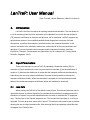
LanTraP: User Manual
Kyle Conrad, Jesse Maassen, Mark Lundstrom
1.
Introduction
LanTraP is an online tool aimed at assisting research and education. The tool allows for
a .txt file containing band structure information to be uploaded, from which the thermoelectric
(TE) transport coefficients for electrons and phonons can be calculated. LanTraP supports any
general band structure, from simplified parabolic/linear dispersions to accurate full band
descriptions, to perform thermoelectric calculations within the Landauer formalism. In this
manual, the basics of the calculation method are outlined and all of the input parameters are
described. For more information about transport and the Landauer formalism, see NearEquilibrium Transport: Fundamentals and Applications, by M. Lundstrom & C. Jeong (World
Scientific, Singapore, 2013).
2.
Input Parameters
There are a few ways to use LanTraP. By uploading a dispersion relation (E(k) for
electrons or E(q) for phonons) the user may then decide to calculate (i) just the distribution of
modes or (ii) calculate the distribution of modes and the transport coefficients simultaneously.
Alternatively the user may upload a distribution of modes file and proceed to calculate the
transport coefficients directly. When the calculation is complete, the tool produces plots and
tables of the modes and transport coefficients (which are available for download).
2.1
Load Data
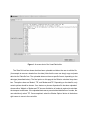
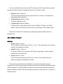
When starting LanTraP this is first slide the user will see. This slide will allow the user to
upload the electron or phonon dispersion (to calculate the thermoelectric properties and/or the
distribution of modes) or a pre-calculated distribution of modes (to calculate the TE properties
only). The first input is the 'Upload' drop down box. This is where the input data (in a .txt file) is
uploaded. From the drop down menu select 'upload'. This selection will prompt a pop up window
allowing the user to select the desired file. After selecting the file and pressing upload the data
will appear in the 'Data file' box.
Figure 1: A screen shot of the 'Load Data' slide.
The 'Data file' text box shows what has been uploaded and allows the user to edit the file
(for example to remove a header from the data). Note that the user can simply copy and paste
data into the 'Data file' box. The uploaded data must have a specific format, depending on the
data type (described below). The final option on this page is the 'What to calculate' drop down
box. The options here are 'Modes', 'TE', and 'Modes and TE'. Depending on the data file, only
certain options should be chosen. If an electron or phonon dispersion file has been uploaded
choose either 'Modes' or 'Modes and TE' since a distribution of modes is required to calculate
the transport coefficients. If the uploaded data was a pre-calculated distribution of modes, the
user should only select 'TE'. Once completed, select the 'Modes Options' button in the bottom
right corner to move to the next slide.
2.1.1 Format for the electron or phonon dispersion file
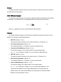
The basic format of a dispersion relation file is the following: each row vector lists the
eigenvalues (in increasing order) corresponding to a specific kx, ky, kz point, with the rows
iterating over all the k-points in the Brillouin zone. The k-grid mesh must be uniform within the
Brillouin zone along a given direction (
to
where is the box size in a given direction), but
the density may be different along kx, ky and kz. Note that the simulation box must be
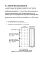
rectangular, with one direction corresponding to the transport direction. By labeling the k-points
by the number from smallest to largest (ikx=1 corresponding to the minimum kx and ikx=nx
corresponding to the max kx) the order of k-points in the dispersion file is as follows (see Figure
2):

Each row corresponds to a list of eigenvalues.

The rows iterate over all the k-points in the Brillouin zone.

The sequence of k-points iterates over kx, ky, kz (in this order).
Figure 2: The proper format for an uploaded dispersion file.
2.1.2 Format for a distribution of modes file
For a pre-calculated distribution of modes the uploaded file has 2 columns, the first is an
energy vector (in eV) in increasing order, and the second is the distribution of modes (in units of
m-(d-1) where d is the dimensionality) at each energy. The output 'Modes Table' from the tool
automatically has the correct format.
2.2
Modes Options
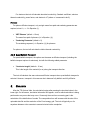
If on the 'Load Data' slide 'TE' was chosen from the 'What to calculate' drop down box, this
slide has no options and prompts the user to select the 'TE Options' button. If from the 'What to
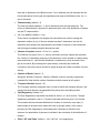
calculate' drop down box either 'Modes' or 'Modes and TE' was selected the user will need to
specify a number of parameters to calculate the modes, displayed on the 'Modes Options' slide.
Figure 3: A screen shot of the 'Modes Options' slide.

'Monkhorst-Pack k-grid?' (default = yes)
The 'Monkhorst-Pack k-grid?' boolean option allows for one of two uniformly spaced kgrid organization schemes to be chosen. The Monkhorst-Pack k-grid is chosen so that
there are no duplicates in the Brillouin zone. If no is selected, the tool assumes that the
first and last points of the k-grid are duplicates at the edge of the Brillouin zone, in kx, ky,
and kz directions.

'Dimensionality' (default = 3)
The user may select between 1, 2, and 3 dimensions from the drop down box. The
choice of dimensionality is important in determining the units of the distribution of modes
and the TE characteristics.

'Lx', 'Ly', and 'Lz' (default = 1 nm)
These values correspond to the lengths of the simulation box used in creating the
dispersion relation (in nm). If the user selects less than 3 dimensions, the tool will
determine which lengths are used based on the number of k-points in each dimension,
with the largest numbers being the dimensions used.

'Number of k-points' (default = 51 for kx, ky, and kz)
The 'Number of k-points' (for kx, ky, and kz) are used to correctly interpret the uploaded
file. If there is no periodicity along any of the directions, set the number of k-points along
those directions to 1. Note that the distribution of modes may not be accurate if the kgrid is too coarse. By increasing the k-point density, eventually the modes will
converge to the correct values and will no longer change with further increases in k-point
density.

'Number of Bands' (default = 1)
Along with 'Number of k-points', 'Number of Bands' is used to correctly interpret the
uploaded file. Note that the number of bands must be the same for all k-points.

'Transport direction' (default = Z)
The 'Transport direction' drop down menu is used to identify the transport direction, and
assigns the other directions as perpendicular k-points when calculating modes.

'Spin Degeneracy' (default = 2)
The 'Spin Degeneracy' drop down box allows for either 1 or 2 to be chosen. The spin
degeneracy parameter is set to 1 (2) when each band should only hold 1 (2) electron.
This ensures that the calculated distribution of modes, for electrons, is per spin (i.e.
identical spin-up and spin-down states will count as a single mode). In the case of
phonons the 'Spin Degeneracy' should always be 2 (different by definition from
electrons, the polarization of phonons is included in the calculation of the distribution of
modes).

'Emin', 'dE', and 'Emax' (default = -1eV, 0.001 eV, 1 eV respectively)
The next 3 options are 'Emin', 'dE', and 'Emax' which allow any value to be entered in
eV. These values determine the energy range (from 'Emin' to 'Emax') as well as the
resolution ('dE') for which modes will be calculated. There will always be 0 modes where
no band exists, so choose the energy range near the range of eigenvalues in the
dispersion. Note that using a 'dE' that is too large may lead to significant errors. Thus, it
is good practice to decrease 'dE' to ensure the distribution of modes is converged and
accurate. Some suggested values are:

Electrons
'dE' should be in the range of 0.01 eV to 0.001 eV

Phonons
'dE' should be in the range of 0.0001 eV to 0.000001 eV
After all of these options have been modified, the 'TE options' button in the lower right
will move the tool onto the next slide.
2.3
TE Options
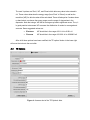
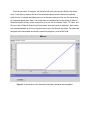
Figure 4: A screen shot of the 'TE Options' slide.
If on the 'Load Data' slide the user chose 'TE' or 'Modes and TE' this slide will have options,
otherwise the slide will show a message that there are no options to modify.

'Particle' (default = Electron)
The 'Particle' drop down box has two options 'Electron' or 'Phonon'. This determines
what properties are calculated.

'Temperature (K)' (default = 300K)
The lattice temperature (in K).

'Transport type' (default = Ballistic)
'Transport type' is a drop down box with choices of 'Ballistic', 'Diffusive', and 'QuasiBallistic', where the last option allows the user to set the length of the transport region.
The choice of 'Particle' and 'Transport type' changes the options available, which are
detailed below.
2.3.1 Ballistic Transport
Electrons

'Ef min' (default = -0.5 eV)
'Ef min' should be chosen such that 'Ef min' > 15 kbT + Emin where Emin is the minimum
energy of the distribution of modes.

'delta Ef' (default = 0.001 eV)
The value of 'delta Ef' is the resolution of the Fermi energy range for which transport
coefficients are calculated over.

'Ef max' (default = 0.5 eV)
'Ef max' should be chosen such that 'Ef max' < Emax -15 kbT where Emax is the
maximum energy of the distribution of modes.
The reason for the restrictions on the Ef-grid is to insure the tool performs a proper
integration. If the Fermi energy range is too wide, an error will occur and the calculation will stop
without completion. For electron ballistic transport the tool will calculate electrical conductance,
Seebeck coefficient, electron thermal conductance, power factor, and electronic zT (where KL is
assumed to be 0).
Phonons
For phonon ballistic transport there are no other options to modify and the tool will calculate
the lattice thermal conductance.
2.3.2 Diffusive Transport
For diffusive transport there are more options, especially when the particle being considered
is an electron. The tool allows for an energy dependent mean-free-path, with the form:
(1)
where
depends on the case considered and is defined below.
Electrons
For electron diffusive transport, all of the options for ballistic transport still need to be set in
addition to the following scattering parameters:

'MFP CB' (default = 10 nm)
The mean-free-path of electrons in the conduction band (

in Equation (1)).
'CB scattering parameter' (default = 0)
The scattering exponent ( in Equation (1)) of the conduction band.

'Conduction Band Minimum' (default = 0 eV)
The minimum energy of the conduction band. For the conduction band,
in Equation (1) where

is the 'Conduction Band Minimum'.
'MFP VB' (default = 10 nm)
The mean-free-path of electrons in the valence band (

in Equation (1)).
'VB scattering parameter' (default = 0)
The scattering exponent ( in Equation (1)) of the valence band.

'Valence Band Maximum' (default = -1 eV)
The minimum energy of the valence band. For the valence band,
in Equation (1) where
is the 'Valence Band Maximum'. The
'Conduction Band Minimum' and 'Valence Band Maximum' are required to be
different values, with 'Valence Band Maximum' being less than 'Conduction Band
Minimum' for the calculation to occur.
For electrons the tool will calculate electrical conductivity, Seebeck coefficient, electron
thermal conductivity, power factor, and electronic zT (where κL is assumed to be 0).
Phonons
For phonon diffusive transport, only a single mean-free-path and scattering parameter are
required, since

in Equation (1).
'MFP Phonon' (default = 10 nm)
The mean-free-path of phonons (

in Equation (1)).
'Scattering Parameter' (default = 0)
The scattering exponent ( in Equation (1)) for phonons.
For phonons, the tool will calculate the lattice thermal conductivity.
2.3.3 Quasi-Ballistic Transport
For quasi-ballistic transport, the options are the same as diffusive transport (including the
ballistic transport options for electrons), but with the following added parameter:

'Conductor length' (default = 10 nm)
This is the length of the material (in nm) along the transport direction.
The tool will calculate the same values as diffusive transport when quasi-ballistic transport is
selected. However, transport in this case can be in between fully ballistic and fully diffusive.
3.
Simulate
After the 'TE Options' slide, the calculation begins after pressing the simulate button in the
lower right. On the screen, simulation information will appear, such as which calculation is being
performed or any errors that may occur. Commonly the most time consuming part is the
calculation of the distribution of modes. The computation time will increase with the size of the
uploaded data file and the resolution of the Fermi energy grid. The tool will typically run for
anywhere between a few seconds to several minutes before completion.
Once the simulation is complete, the final slide will have a plot and the 'Result' drop down
menu. From the drop down menu all of the calculated values can be selected to be plotted
within the tool. If multiple simulations were run in the same instance of the tool, the results may
be compared against each other. If an output was not calculated due to the choice of 'What to
calculate' the plot will only contain one point at (0,0). As well, the 'Modes Table', 'TE Table', and
'Phonon Lattice Thermal Conductivity/Conductance' show the results in table form. Each output
may be downloaded from the tool using the button next to the 'Result' drop down. The tables are
designed to be downloaded and directly loaded into programs, such as MATLAB.
Figure 5: A screen shot of the 'Simulate' slide after calculation has completed.