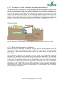
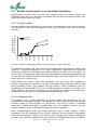
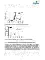
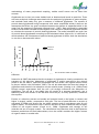
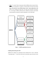
1
Bioforsk Rapport Bioforsk Report Vol. 8 Nr. 172 2013 National Scenarios - Norway Development of WISPE for surface- and groundwater modelling of pesticides in major crops Randi Iren Bolli1, Ole Martin Eklo1, Roger Holten2, Paulien Mulder2 1 Bioforsk, Plant Health and Plant Protection Division Norwegian Food Safety Authority 2 Head office Frederik A. Dahls vei 20 N-1430 Ås Tel.: (+47) 40 60 41 00 [email protected] Bioforsk Plant Health and Plant Protection Division Høgskoleveien 7 1432 Ås Tel.: (+47) 40 60 41 00 [email protected] Title: National Scenarios – Norway Development of WISPE for surface- and groundwater modelling of pesticides in major crops Author(s): Randi Iren Bolli, Ole Martin Eklo, Roger Holten, Paulien Mulder Date: Availability: Project No.: Archive No.: 16/12-2013 Open 1110330 2007/118 Report No.: ISBN-no: Number of pages: Number of appendices: 8(172) 2013 978-82-17-01184-2 61 1 Employer: Contact person: Norwegian Food Safety Authority Roger Holten Keywords: Field of work: WISPE, pesticides, modelling, national scenarios Pesticide fate Sammendrag: Dette arbeidet er en videreføring av prosjektet Norske Scenarier. Formålet med prosjektet var å inkludere de mest utbredte jordbrukskulturene til modellverktøyet WISPE, å utvide modellen med en funksjon som beregner eksponering av plantevernmidler til ulike vannmiljø og kalibrere modellen med hensyn på transport av partikler og partikkelbundne plantevernmidler. Prosjektet har vært et samarbeid mellom Bioforsk Plantehelse, Waterborne Environmental Inc. og Mattilsynet. Summary: This work is a continuation of the project Norwegian Scenarios. The aim of this project was to include the major crops in Norway to the model tool WISPE, to extend the model with an aquatic fate model and to make a better model adaption regarding transport of soil particles and particle bound pesticides. This project has been a cooperation between Bioforsk Plant Health and Plant Protection Division, Waterborne Environmental Inc. and Norwegian Food Safety Authority. Approved Project leader Børge Holen Ole Martin Eklo Preface This project has been a cooperation between Bioforsk Plant Health and Plant Protection Division, Waterborne Environmental Inc. and Norwegian Food Safety Authority. The project has been carried out as an assignment from the Norwegian Food Safety Authority. The aim of the project was to include the major crops in Norway into the scenarios from Bjørnebekk and Syverud to the model tool WISPE, to extend the model with an aquatic fate model (EXAMS) and to make a better model adaption regarding transport of soil particles and particle bound pesticides. Bioforsk Plant Health and Plant Protection Division have been responsible for the coordination, implementing of crops and calibration of soil loss and particle bound pesticides. Waterborne Environmental Inc. has been responsible for the software development, user manual of WISPE and the implementation of EXAMS. Project associates have been Randi Bolli and Ole Martin Eklo (project coordinator) from Bioforsk Plant Health and Plant Protection Division, Amy Ritter and Mark Cheplick from Waterborne Environmental Inc. and Roger Holten and Paulien Mulder from the Norwegian Food Safety Authority. Contents Preface .................................................................................................... 3 Contents .................................................................................................. 4 1. Summary ............................................................................................ 5 2. Sammendrag ........................................................................................ 6 3. Introduction ........................................................................................ 7 4. Exposure of pesticides in aquatic systems ..................................................... 9 5. Crop scenarios .................................................................................... 11 6. Transport of particles and particle bound glyphosate ...................................... 14 6.1 Materials and methods .................................................................... 14 6.1.1 Field description ....................................................................... 14 6.1.2 Treatment of sites, sampling procedure and analysis ............................ 15 6.1.3 Model and parameter estimation.................................................... 15 6.2 Results and discussion from the model simulations ................................... 16 6.2.1 Surface water .......................................................................... 16 6.2.2 Sediment loss .......................................................................... 16 6.2.3 Dissolved and particle bound glyphosate in surface water ...................... 17 6.2.4 Sediment loss and dissolved/particle bound glyphosate from Bjørnebekk .... 20 7. Conclusion ........................................................................................ 21 8. References ........................................................................................ 22 9. Appendix .......................................................................................... 24 Bolli, R.I. et al. Bioforsk Report vol. 8 nr. 172 2013 4 1. Summary Waterborne Environmental Inc. has together with Bioforsk, as an assignment from the Norwegian Food Safety Authorities, developed the risk assessment tool WISPE (The World Integrated System for Pesticide Exposure) which includes several environmental fate and transport models. WISPE is a computer modelling tool developed to evaluate the potential for pesticides to occur in aquatic environments. The scenarios Bjørnebekk and Syverud are included in WISPE which makes it possible to estimate pesticide exposure in surface- and groundwater resources considering Norwegian conditions. The first sub-goal has been to include an aquatic fate model into WISPE to predict exposure to aquatic living organisms. WISPE has been extended with EXAMS (The Exposure Analysis Modeling System), which is the U.S. standard model used to calculate the PEC (predicted environmental concentrations) values of pesticide discharge into a standard water body (pond, ditch or stream). This is similar to TOXSWA (TOXic substances in Surface Waters), which is a part of the FOCUS surface water exposure assessment. The second sub-goal has been to extend the model to major crops in Norway, taking into consideration the effect of the climate on the plant growth development including sowing, emergence and harvest. The third sub-goal was to calibrate PRZM (Pesticide Root Zone Model) according to transport of particles and particle bound pesticides, especially glyphosate, with existing field data. PRZM simulates the amount of surface water and soil loss from the Askim field adequately, and the results are within the acceptability limit for the deviation between simulated and observed values. Similar to earlier simulations with PRZM, also here there were problems in periods characterized by frozen soil, freezing and thawing cycles, and high surface runoff during snowmelt events (Eklo et al., 2008, Eklo et.al. 2009, Bolli et al., 2011). Glyphosate can be transported into water bodies both as dissolved and bound to particles. Pesticide losses in surface runoff are “event-driven” and therefore very strongly dependent on the weather conditions, especially rainfall immediately after application. There was a good correlation between the total simulated amount of dissolved glyphosate (34 mg) and the observed values (24 mg). The simulation indicated that the model did not time the runoff events well, which can be related to the daily resolution of the meteorological data. The model simulates too much loss of particle bound glyphosate compared to the calculated values. Erosion is a selective process and eroded soil materials tend to consist of smaller particles and higher content of organic carbon. Adsorption of glyphosate is mainly governed by the mineral phase of the soil matrix and not to the organic matter. PRZM uses an enrichment ratio to account for that eroded soils have a higher content of soil organic matter, which can lead to more inaccurate simulations of particle bound glyphosate due to the strong sorption to soil minerals. The soil properties for the Askim site are quite similar to the soil from Bjørnebekk, and the parameters used for the sediment loss calibration at Askim were also used for Bjørnebekk. The simulation showed that the cumulative simulated values were high compared to the calculated values, 91 kg and 3 kg respectively. These simulations confirmed that transfer of data from one site to another is not recommended since the soil properties and topography strongly influence the model simulations. Thus, the model has to be calibrated with the field properties that are found at each site (pers. comm. Cheplick, 2013). Bolli, R.I et al. Bioforsk Report vol. 8 nr. 172 2013 5 2. Sammendrag Waterborne Environmental Inc. har sammen med Bioforsk og på oppdrag fra Mattilsynet, utviklet risikovurderingsverktøyet WISPE (The World Integrated System for Pesticide Exposure) som inkluderer både transportmodeller og modeller som beregner eksponeringen av plantevernmidler i ulike vannmiljø. De norske scenariene fra Bjørnebekk og Syverud er inkludert i WISPE, noe som gjør det mulig å gjøre risikovurderinger i overflate- og grunnvannsressurser med hensyn på norske forhold. Det første delmålet i prosjektet var å inkludere en modell som kunne beregne plantevernmiddel eksponeringen for vannlevende organismer. WISPE har blitt utvidet med EXAMS (The Exposure Analysis Modeling System) som er standard modellen i USA for beregning av PEC (predicted environmental concentrations) verdier til plantevernmidler sluppet ut i et standard vannmiljø (pond, ditch, stream). EXAMS har de samme egenskapene som modellen TOXSWA (TOXic substances in Surface Waters), som brukes i risikovurderingsarbeidet i Europa. Det andre delmålet i prosjektet var å inkludere i modellen de mest utbredte jordbrukskulturene i Norge slik at det norske klimaet blir tatt hensyn til i forhold til planteutvikling, noe som inkluderer såing, modning og høsting. Det tredje delmålet var å bruke eksisterende norske feltdata fra Askim til å kalibrere PRZM (Pesticide Root Zone Model) med hensyn på transport av partikler og partikkelbundne plantevernmidler (glyfosat). Modellen viste god tilpassing mellom predikerte og observerte verdier både av overflatevann og jordtap. Som tidligere simuleringer med PRZM har vist, var det også her problemer i perioder som ofte er karakterisert av frossen jord, frysing/tining og stor overflateavrenning under snøsmeltingen (Eklo et al. 2008, Eklo et.al. 2009, Bolli et al. 2011). Glyfosat kan tapes i både løst og partikulær form. Tidspunkt og intensitet av nedbørsepisoder i forhold til sprøytetidspunktet er av stor betydning for hvordan plantevernmidlene transporteres. Det var god tilpassing mellom total mengde løst glyfosat (34 mg) og de observerte verdiene (24 mg). Simuleringen viste at modellen hadde problemer med tidspunktet for avrenningen, noe som kan skyldes at daglige verdier blir brukt i klimafilen. Modellen overestimerte avrenningen av partikkelbundet glyfosat. Erosjon er en selektiv prosess og erodert jord består ofte av mindre partikler og et høyere innhold av organisk karbon. Adsorpsjon av glyfosat skjer hovedsakelig til mineraldelen av jorda, og ikke til organisk materiale. Siden erodert jord ofte har et høyere innhold av organisk karbon enn utgangsmaterialet bruker PRZM en faktor (enrichment ratio) for å ta hensyn til dette i beregningene av mengde partikkelbundet glyfosat, noe som kan gi et avvik mellom simulerte og observerte verdier. Jordegenskapene for Askim er ganske lik jorda på Bjørnebekk, og derfor ble parameterne som ble brukt for kalibrering av jordtapet på Askim også brukt for Bjørnebekk. Simuleringene viste at de kumulative predikerte verdiene var høye sammenlignet med de beregnede observerte verdiene, henholdsvis 91 kg og 3 kg. Disse simuleringene har bekreftet at overføring av data fra et sted til et annet ikke er å anbefale siden jordegenskapene og topografien påvirker modellsimuleringene. Modellen må derfor kalibreres med data for hvert enkelt felt (pers. med. Cheplick, 2013). Bolli, R.I. et al. Bioforsk Report vol. 8 nr. 172 2013 6 3. Introduction The contamination of surface water bodies with agricultural pesticides can pose a significant threat to aquatic ecosystems, and has increased the need for tools which can predict the behaviour of chemicals entering the environment. Such a tool is The World Integrated System for Pesticide Exposure (WISPE) which is a modelling platform designed to evaluate the potential for pesticides to occur in surface- and groundwater resources. The structure of the model allows seamless executions of several environmental fate and transport models in the Windows environment and it also has the flexibility for the user to create, update and maintain databases on pesticides environmental fate properties and exposure scenarios (Cheplick et al., 2012). The following simulation models have been implemented into WISPE: PRZM (Pesticide Root Zone Model): Surface- and groundwater scenarios for different crops require simulations of PRZM for the terrestrial field. PRZM is a dynamic compartment model which can be used to simulate chemical movement in unsaturated soil systems within and below the root zone (Carsel et al., 2006). PRZM is used for pesticide risk assessments by the U.S. Environmental Protection Agency’s Office of Pesticide Programs (USEPA, 2007) and for pesticide risk assessment work in Europe and Canada (FOCUS, 2005; FOCUS, 2004; PMRA, 2003). WISPE uses Win-PRZM (version 4.5., April 2009) which is used for pesticide registration in Europe. Win-PRZM contains parts which is unavailable in the version published by the USEPA such as the Freundlich adsorption isotherm, aged sorption and soil moisture dependent degradation. RICEWQ (The Rice Water Quality Model): The RICEWQ model simulates the pesticide mass balance and water management practices in rice paddy environments (Williams et al., 2008). This part of the WISPE model is not activated for the Norwegian version. EXAMS (The Exposure Analysis Modeling System): The EXAMS model is a chemical fate and transport model combined with a hydraulic model which simulates different processes in aquatic environments (Burns et al., 2004). For the U.S. Environmental Protection Agency’s Office of Pesticide Programs (USEPA, 2007), EXAMS is the standard model used for ecological and drinking water pesticide risk assessments. ADAM (The Aquifer Dilution Assessment Model): The ADAM model predicts chemical dilution, partitioning and persistence in a shallow, unconfined aquifer receiving daily recharge water and chemical flux from PRZM (Williams, 2010). Water displacement in the aquifer is from recharge and lateral flow. The connection between PRZM and ADAM has been validated to groundwater monitoring studies conducted for pesticide registration in the United States. WISPE has had some changes since the User Manual was made in December 2012 (Cheplick et al., 2012). One of the changes is the Scenario Manager which allows us to implement our own scenarios into the WISPE software. This is a very useful tool, which makes us capable to do this work ourselves in an easy way. Waterborne Environmental Inc. has included the Norwegian surface- and groundwater scenarios from Bjørnebekk and Syverud (Eklo et al., 2008, Eklo et.al. 2009, Bolli et al., 2011) into WISPE, which makes it possible to do pesticide exposure assessments in surfaceand groundwater resources considering Norwegian conditions. A part of this project was to include the major crops into WISPE to make it more representative for Norway. The crop Bolli, R.I et al. Bioforsk Report vol. 8 nr. 172 2013 7 grown at each scenario and the practices used to manage the soil, contribute to a potential exposure of pesticides to surface water bodies. The size of the crop canopy influences the amount of pesticides reaching the soil, and the depth and distribution of root systems together with soil management practices affect the soil water balance and therefore indirectly the amount of runoff and drain flow (FOCUS, 2001). The major transport pathway for soil particles and particle bound pesticides is surface runoff, which to a large extent depends of soil properties and hydrological characteristics. Transport of particles and particle bound pesticides like glyphosate, is particularly affected by tillage, rainfall intensity, timing of rainfall in relation to spraying, and the interval between two rainfall events. The transport of pesticides is also affected by pesticide properties such as solubility, sorption and degradation. Uneven soil surface, soil with high content of organic carbon, high aggregate stability and porosity, as well as crop residues covering the soil, will reduce erosion and losses of pesticides to surface waters. In the south eastern part of Norway the erosion and transport of particle bound pesticides are highest during winter and spring. These transport processes are heavily dependent on climatic conditions and especially precipitation events shortly after application and melting-freezing episodes during winter. Bolli, R.I. et al. Bioforsk Report vol. 8 nr. 172 2013 8 4. Exposure of pesticides in aquatic systems There are many models available that are able to estimate the fate of a substance in different environmental compartments after its application in agriculture. The FOCUS Working Group on Surface Water Scenarios has chosen a specific set of models to account for the different contamination routes of surface waters. The models chosen are MACRO for estimating the contribution of drainage, PRZM for the estimation of the contribution of runoff and TOXSWA for the estimation of the final predicted environmental concentration (PEC) in surface waters (FOCUS, 2001). TOXSWA (TOXic substances in Surface Waters) is an aquatic fate model and does not simulate the drainage or runoff/erosion processes itself, but uses the fluxes calculated by other models as entries into the water body system. TOXSWA uses these output files as input to calculate exposure in water and in sediment at the downstream end of a ditch, stream or pond neighboring a treated field. TOXSWA considers the transport processes (advection, dispersion), transformation (hydrolysis, photolysis, biodegradation), sorption and volatilization (figure 1) (FOCUS, 2001). FOCUS Pond scenario 4500 m2 field treated with Inputpesticide from drainage or runoff plus baseflow with no pesticide Pond FOCUS Ditch Pond outflow regulated by a broadScenariocrested weir with a height of 1.0 m Eroded sediment (+ pesticide) input from a 20 m contributing margin along one side of pond (runoff scenarios only) 2 hectare field, not treated Input from drainage and baseflow (20 ha for D2) 100 m 1 hectare field treated with pesticide Input from drainage only FOCUS Stream Scenario Minimum water depth of 0.3 m maintained by a weir 100 ha upstream catchment. 20 % treated with pesticide Input from drainage or runoff plus baseflow with no pesticide. Eroded sediment (+ No sediment input pesticide) input from a 20 m 1 ha field treated contributing margin along with pesticide stream 100 m Input from (runoff scenarios only) drainage or runoff Minimum water depth of 0.3 m maintained by a weir Figure 1. Conceptual outline of the FOCUS surface water bodies (FOCUS, 2001) Bolli, R.I et al. Bioforsk Report vol. 8 nr. 172 2013 9 Because of problems with coupling WISPE and TOXSWA it was decided to combine the field scale runoff/leaching model PRZM with the surface model EXAMS in WISPE. EXAMS is the U.S. equivalent to TOXSWA with similar capabilities (USEPA, 2007). Like TOXSWA, EXAMS calculates the pesticide exposure in three different aquatic environments; pond, stream and ditch (figure 1). PRZM connected with EXAMS are the standard models used for ecological and drinking-water risk assessment for pesticides by the U.S. Environmental Protection Agency’s Office of Pesticide Programs (USEPA, 2007). PRZM produces runoff and erosion values that represent volumes and concentrations that are likely to be observed at the edge of the agricultural field. Each PRZM modelling scenario represents a combination of climatic conditions, crop specific management practices, soil specific properties, site specific hydrology, and pesticide specific application and dissipation processes. Each PRZM simulation is conducted using multiple years of rainfall data to cover year-to-year variability in runoff. Daily edge-of-field loadings of pesticides dissolved in runoff waters and sorbed to entrained sediment are discharged into a standard water body (pond, stream or ditch) simulated by the EXAMS model. EXAMS simulates the processes that occur in the water body rather than on the agricultural field. The EXAMS model accounts for hydrologic transport, volatilization, sorption, hydrolysis, biodegradation and photolysis of the pesticide. EXAMS takes the runoff and spray drift loading generated by PRZM and estimates the concentration of pesticides in the water body on a day-to day basis. The combination of substance specific data, scenario specific data and crop specific data result in an estimated environmental concentration (EEC) in surface water that is used for the risk assessment processes. More information can be obtained in the manuals for PRZM, EXAMS and WISPE (Carsel et al., 2006, Burns, 2004, Cheplick et al., 2012). In order to run the TOXSWA in FOCUS model, a set range of characteristics relating to the dimensions, sediment and organic components and hydrology of each water body are required to parameterize each scenario. It was important that the definitions in EXAMS were similar to the definitions in TOXSWA. Table 1 gives an overview over some important parameters that are similar between EXAMS and TOXSWA. Table 1. Parameters in EXAMS that is similar to TOXSWA Ditch Pond Width (m) 1 30 Total length (m) 100 30 Average water depth (m) 0.3 1 Concentration of suspended solids (mg/L) 15 15 Organic carbon content (%) 5 5 Dry bulk density (kg/m3) 800 800 Stream 1 100 0.3 15 5 800 More information about the parameters in EXAMS and TOXSWA can be found in the EXAMS manual (Burns et al., 2004) and the FOCUS document (FOCUS, 2001). Bolli, R.I. et al. Bioforsk Report vol. 8 nr. 172 2013 10 5. Crop scenarios In WISPE, the Norwegian scenarios from Bjørnebekk and Syverud have been calibrated for spring barley, which is one of the most common crops in Norway. An important part of this project was to implement other major crops into WISPE to make it more relevant for Norway. Table 2 shows the most widespread crops in Norway with dates for sowing, emergence and harvest. The collection of data regarding plant growth development for the main crops were received from the Norwegian Agricultural Extension Service, department Hedmark (potatoes, onion), SouthEast (cereals, oilseed, legumes) and Viken (vegetables, fruit, berries) (Eklo et al., 2008). Table 2. An overview over the main crops in Norway Cereals, winter Sowing date 8/9 Emergence date Harvest date Spring oilseed Sowing date Emergence date Harvest date Potatoes Sowing date Emergence date Harvest date Vegetables, root (Carrots) Sowing date Emergence date Harvest date Vegetables, leafy (Cabbage) Sowing date Emergence date Harvest date Vegetables, bulb (Onions) Sowing date Emergence date Harvest date Strawberries Emergence date Harvest date Freezing date Bush berries Emergence date Harvest date Freezing date 15/9 15/8 1/5 10/5 4/9 20/5 10/6 20/9 10/5 25/5 5/10 15/5 30/5 15/9 28/4 17/5 28/8 23/4 8/7 20/10 23/4 15/8 20/10 Bolli, R.I et al. Bioforsk Report vol. 8 nr. 172 2013 11 Orchard Emergence date Harvest date Freezing date Legumes Emergence date Harvest date 23/4 18/9 20/10 10/5 20/8 The selection of crop and management factors is an essential component of the derivation of input parameters (FOCUS, 2001). For instance, crop interception will decrease the amount of pesticides that reach the soil surface and thus ultimately enter the surface water body via runoff or drainage. Crop and management input parameters were selected for the PRZM model for each crop in the surface- and groundwater scenarios from Bjørnebekk and Syverud. Input parameters specific for each crop were: Maximum interception storage of crop Maximum rooting depth of crop Maximum area coverage of canopy Maximum canopy height at maturation date Runoff curve number Dates for sowing, emergence, maturation and harvest The remaining parameters were constant. Parameter selection for each crop was based on local information (table 2), the PRZM manual (Carsel et al., 2006), expert judgements and the FOCUS scenarios from Jokioinen. When the selection of the FOCUS scenarios was made, Europe was classified in different regions according to precipitation and temperature (figure 2). Climate region (FOCUS) 1 = 0-5 °C, < 400 mm 2 = 0-5 °C, > 400 mm 3 = 5-10 °C, < 400 mm 4 = 5-10 °C, > 400 mm Figure 2. Climate regions based on air temperature and precipitation. The average annual air temperature and average annual precipitation are shown in the legend (Lars Egil Haugen, personal communication, 2005). Bolli, R.I. et al. Bioforsk Report vol. 8 nr. 172 2013 12 The classification shows that the south eastern part of Norway is in the same region as the mid part of Sweden and the main part of Finland (climate region 1). The Finnish scenario Jokioinen, together with Bjørnebekk and Syverud, is located in climate region 1, which is characterized as a relatively dry and cold climate. Bolli, R.I et al. Bioforsk Report vol. 8 nr. 172 2013 13 6. Transport of particles and particle bound glyphosate A part of this project was to calibrate PRZM to achieve a better adaption of the sediment loss and the loss of pesticides which sorbs strongly to soil particles, i.e. glyphosate. Glyphosate can be transported in soil as dissolved or bound to particles. Results from monitoring glyphosate through the Norwegian (JOVA) and the Swedish pesticide monitoring programs indicate that glyphosate is mainly lost through transport with soil particles. In catchments and during runoff episodes with large particle losses, also large amounts of glyphosate are lost (Stenrød et al., 2007). 6.1 Materials and methods The calibration of PRZM was performed with data from controlled plot studies at the sites Askim, Bjørnebekk and Syverud. Data for suspended solids, turbidity and dissolved glyphosate was achieved from the study at Askim. Since there were no data describing the amount of suspended solids from Bjørnebekk and Syverud, data from Askim was used to calculate the amount of suspended solids in surface water using turbidity measurements from the other sites. Information about Bjørnebekk and Syverud are thoroughly described in earlier reports (Eklo et al., 2008, Eklo et.al. 2009 and Bolli et al., 2011). The field experiment at Askim was conducted by the Norwegian University of Life Sciences (Stenrød et al., 2007). 6.1.1 Field description Runoff of the pesticide glyphosate and its metabolite AMPA (aminomethylphosphonic acid) has been investigated in plot studies in an agricultural field at Askim. The field was artificially levelled, tile drained and established in 1986. The experimental plots are 26 m long and 6.2 m wide with a slope of 13 % (figure 3). The soil is a silty clay loam with a low content of organic carbon, poor aggregate stability and high erodibility (Stenrød et al., 2007). Figure 3. The experimental field at Askim (Source: Riise et al., 2012) Bolli, R.I. et al. Bioforsk Report vol. 8 nr. 172 2013 14 6.1.2 Treatment of sites, sampling procedure and analysis The plots at Askim were subject to autumn ploughing and spring ploughing. All plots were subject to harrowing in spring. The pesticide glyphosate were applied in September and the tracer kaliumbromide (KBr) was applied at the same time to follow the transport of water. Water proportional samples with a tipping bucket system were collected from both surface- and drainage water (figure 4). The sampling frequency varied from one to five weeks depending on volume of runoff. Analyses of glyphosate and AMPA were conducted at Bioforsk, Plant Health and Plant Protection. Measurements of suspended solids (SS) and turbidity was done by the Norwegian University of Life Sciences (Stenrød et al., 2007.). Figure 4. Illustration of the sampling of water proportional samples (Source: Riise et al., 2012) 6.1.3 Model and parameter estimation PRZM was used for calibration of sediment loss and particle bound pesticides from the experimental fields. A detailed description of PRZM can be achieved from the manual (Carsel et al., 2006) and from earlier reports (Eklo et al., 2008, Eklo et.al. 2009 and Bolli et al., 2011). The parameter estimation was performed at two stages: an uncalibrated simulation followed by a simulation with calibration using the sensitive parameters. The hydrology module is always calibrated first and the pesticide module last. This is important, as water is the carrier of pesticides through the soil. Knowledge of the water flow is therefore a prerequisite of a valid description of the movement of pesticides in soil. This is a suggested procedure of Good Modelling Practice (GMP) obtained in the Cost Action 66 project (Vanclooster et al., 2000). There were three main sources for the parameter estimations; measurements or calculation based on measurements, the PRZM manual, other literature sources and expert judgement. Bolli, R.I et al. Bioforsk Report vol. 8 nr. 172 2013 15 6.2 Results and discussion from the model simulations Measurements of water flow from both the drainage system and surface runoff were measured at the plot. For calibration of sediment loss and particle bound pesticides, only data from surface runoff were used. 6.2.1 Surface water Various strategies were attempted in order to get a good adaption of the runoff (figure 5). The parameter which had the biggest influence on the water flow was the rainfall intensity. Surface runoff (mm) 80 Simulated Observed 70 60 50 40 30 20 10 Apr-07 Mar-07 Feb-07 Jan-07 Dec-06 Nov-06 Oct-06 Sep-06 Aug-06 0 Figure 5. Cumulative calibrated simulation of surface water at Askim, 2006-2007 The difference between the total amount of simulated water and observed values were about 25 %. According to Resseler et al. (1996) a satisfactory simulation occurs when the difference between the simulated and observed amount of water do not exceed 25 % during a year. Reichenberger (2005) did some considerations about the acceptability limit for the deviation between simulated and measured values, and according to this, surface runoff was set to a factor of 10. PRZM predicts the surface water flow adequately, but there were some problems in periods characterized by frozen soil, freezing and thawing cycles and high surface runoff during snowmelt events. This problem was also found in earlier simulations done for Bjørnebekk and Syverud (Bolli et al., 2011). PRZM considers the effect of snowmelt in the runoff equation, but the curve numbers are not adjusted to account for the effects of snowpack or frozen ground on runoff generation (Reichenberger, 2005). 6.2.2 Sediment loss The sediment loss is highly dependent on erosion which again depends on the soil permeability and aggregate stability. Topographical conditions like the land slope and the hydraulic length is also important for the erosion. Soil loss by erosion is modelled empirically in PRZM using MUSS, a modification from the Modified Universal Soil Loss Equation (MUSLE), which is specifically designed for small watersheds. After recommendations from the model developer (pers. comm. Cheplick, 2013), parameters like the topographic factor USLELS (universal soil loss equation topographic factor) and the hydraulic length of the field (HL) were changed to get a better adaption of the data. The difference between the total amount of simulated and observed sediment Bolli, R.I. et al. Bioforsk Report vol. 8 nr. 172 2013 16 loss was about 9 % (figures 6 and 7). The timing of the largest runoff event and the amount simulated was very good. The simulated amount of sediment loss was 11 kg, while the observed amount was 9 kg. Sediment loss (kg) 12 Simulated Observed 10 8 6 4 2 Apr-07 Mar-07 Feb-07 Jan-07 Dec-06 Nov-06 Oct-06 Sep-06 Aug-06 0 Figure 6. Calibrated simulation of sediment loss at Askim, 2006-2007 Sediment loss, cumulative (kg) 25 Simulated Observed 20 15 10 5 Apr-07 Mar-07 Feb-07 Jan-07 Dec-06 Nov-06 Oct-06 Sep-06 Aug-06 0 Figure 7. Cumulative calibrated simulation of sediment loss at Askim, 2006-2007 6.2.3 Dissolved and particle bound glyphosate in surface water Glyphosate is quite easily soluble in water, but the risk of leaching has been regarded as low due to its relatively fast degradation in soil and strong sorption to soil particles. Particle bound pesticides are generally believed to have a lower potential to leakage to watercourses than pesticides with lower affinity to soil (Wauchope, 1978). Sorption of pesticides to soil is an equilibrium reaction which is dependent on the soil/water ratio and the contact time between pesticide and soil. During transport of glyphosate with soil particles to surface- and drainage water, a major change of soil/water ratio occurs and the glyphosate molecules might be released from the soil particles. The total amount of simulated dissolved glyphosate (34 mg) lost to the surface water is quite similar to the observed amount (28 mg) (figure 8 and 9). The simulated pesticide runoff losses are affected by uncertainty from both water transport and chemical transport Bolli, R.I et al. Bioforsk Report vol. 8 nr. 172 2013 17 25 Simulated Observed 20 15 10 5 Apr-07 Mar-07 Feb-07 Jan-07 Dec-06 Nov-06 Oct-06 Sep-06 0 Aug-06 Dissolved glyphosate (mg) simulation. The deviation between simulated and measured values can thus be expected to be higher for pesticide runoff than for the corresponding runoff water volumes. However, for the purpose of aquatic risk assessment, an under or over prediction of pesticide inputs into a surface water body by more than a factor of 10 cannot be considered as acceptable (Reichenberger et al., 2005). Figure 8. Calibrated simulation of dissolved glyphosate in surface water at Askim, 2006-2007 Dissolved glyphosate, cumulative (mg) 40 Simulated Observed 35 30 25 20 15 10 5 Apr-07 Mar-07 Feb-07 Jan-07 Dec-06 Nov-06 Oct-06 Sep-06 Aug-06 0 Figure 9. Cumulative calibrated simulation of dissolved glyphosate in surface water at Askim, 2006-2007 The timing of the runoff events do not fit well with the observed measurements (figure 8). Pesticide losses in surface runoff are event-driven and therefore very strongly dependent on the weather conditions immediately after application, in particular the rainfall pattern. Earlier simulations have showed that the model has the tendency to under predict for high intensity rainfalls and large runoff/erosion events (Bolli et al., 2011). According to Reichenberger (2005), this is probably due to the daily calculation step of PRZM and that the model does not consider actual rainfall. Meteorological data used for environmental fate modelling generally consists of daily values for precipitation, temperature and evapotranspiration. The daily resolution of weather data is used primarily because daily data is easier to obtain than data with finer temporal resolution. For transient processes such as runoff and erosion, which have time scales of minutes to days, the use of daily weather creates significant uncertainties (FOCUS, 2001). Sampling procedures from field experiments are important for the interpretation of the observed results. Due to the Bolli, R.I. et al. Bioforsk Report vol. 8 nr. 172 2013 18 methodology of water proportional sampling, sudden runoff events are not taken into account. 100 Simulated Observed 80 60 40 20 Apr-07 Mar-07 Feb-07 Jan-07 Dec-06 Nov-06 Oct-06 Sep-06 0 Aug-06 Particle bound glyphosate (mg) Glyphosate can be lost into water bodies both as dissolved and bound to particles. There are some analytical challenges associated with the analysis of glyphosate in water samples, and methods used today only give a measure of dissolved glyphosate. The amount of particle bound glyphosate being transported with water (suspended solids) is built on the assumption that there is a good correlation between the amount of suspended solids in the water and the amount of glyphosate (Stenrød et al., 2007). Data collected for suspended solids from the Askim field were used together with results for dissolved glyphosate and Kd to calculate the amount of particle bound glyphosate. The model simulates too much loss of particle bound glyphosate according to the calculated values (figure 10). It is difficult to decide whether the calculations of particle bound glyphosate is better than the simulations or not due to inaccurate Kd values. Figure 10. Calibrated simulation of particle bound glyphosate in surface water at Askim, 2006-2007 Stenrød et al (2007) documents that the transport of glyphosate is closely connected to the transport of soil particles. Adsorption of glyphosate is mainly governed by the mineral phase of the soil matrix, especially aluminium and iron oxides. Soil organic matter seems to play an indirect role (Vereecken, 2005). The soil pH determines the electrical charge of glyphosate and therefore its adsorption on the mineral phase. Gimsing et al. (2004) found through several experiments that the soil’s pH strongly influenced the adsorption of glyphosate. The soil pH is not added into the model as a separate parameter, but is indirectly taken into account in the Kd value since the pH, for many pesticides, influences the sorption. Erosion is a selective process and eroded soil material tends to be lighter in texture and higher in organic carbon, compared to field soils. The loss of pesticides due to erosion is expressed in PRZM with factors like the MUSS equation and an enrichment ratio for soil organic matter. The enrichment ratio is used to account for that eroded soils have a higher content of soil organic matter (Carsel et al., 2006). Glyphosate sorb strongly to soil minerals and not to organic matter. The calculations may therefore lead to discrepancies between predictions and field observations, since the model considers the higher content of organic matter in eroded soils. Bolli, R.I et al. Bioforsk Report vol. 8 nr. 172 2013 19 6.2.4 Sediment loss and dissolved/particle bound glyphosate from Bjørnebekk The parameters used for calibration of the Askim site regarding sediment loss and transport of glyphosate to the surface water, were also used for the simulations from Bjørnebekk since the soil from Askim is quite similar to the soil from Bjørnebekk. The sediment data from Bjørnebekk was limited to only turbidity measurements. Turbidity is a measure of water clarity, i.e. how much the suspended particles in water decrease the light transmission in the water. The more total suspended solids in the water, the higher the turbidity. Measured values of the amount of suspended solids present are more reliable than turbidity. Since there were no data describing the amount of suspended solids from Bjørnebekk, data from Askim was used to calculate the amount of suspended solids in the surface water. The simulation indicated high values compared to the calculated values, 91 kg and 3 kg respectively. This exercise confirms that the transfer of data from one site to another is not recommended as the properties of soil and topography strongly influence the model simulations. Thus, the model has to be calibrated with the field properties (soil, topography etc.) that are found at each site (pers. comm. Cheplick, 2013). Based on this experience, Syverud was not calibrated as values for suspended solids were lacking and the soil properties were different compared to Askim. Bolli, R.I. et al. Bioforsk Report vol. 8 nr. 172 2013 20 7. Conclusion Pesticide losses from agricultural fields can pose a significant threat to water bodies, and one has seen the need for tools which can predict the exposure of pesticides in both surface- and groundwater. WISPE is a computer modelling tool developed to evaluate the potential for pesticides to occur in aquatic environments. The model has been extended to eleven different crops taking into consideration the effect of the climate on the plant growth development including sowing, emergence and harvest. WISPE has been extended with EXAMS, which is the U.S. standard model used as an aquatic fate model to calculate the PEC values of pesticide discharge into a standard water body (pond, ditch or stream). This is similar to TOXSWA, which is a part of the FOCUS surface water exposure assessment. PRZM simulates the amount of surface water and soil loss from the Askim field adequately, and the results are within the acceptability limit for the deviation between simulated and observed values. As earlier simulations from Bjørnebekk and Syverud have shown, the model encounters difficulties when estimating exposure in periods with frozen soil, freezing and thawing cycles and high surface runoff during snowmelt events (Eklo et al., 2008, Eklo et.al., 2009, Bolli et al., 2011). Glyphosate can reach water bodies both in a dissolved state and bound to particles. The total simulated amount of dissolved glyphosate (34 mg) lost to surface water was similar to the observed amount (24 mg). The simulation showed that the model did not time runoff events well compared to the observed measurements. The model simulates too much loss of particle bound glyphosate compared to calculated values, due to the strong sorption of glyphosate to soil minerals and not to the organic matter. Transfer of data from one site to another is not recommended since the soil properties and topography strongly influence the model simulations. Thus, the model has to be calibrated with the field properties that are found at each site (pers. comm. Cheplick, 2013). The effect of soil particles on transport and analytical determination of glyphosate should be further investigated to give increased knowledge on the behaviour of glyphosate in a soil-sediment-water system. Bolli, R.I et al. Bioforsk Report vol. 8 nr. 172 2013 21 8. References Bolli, R.I., Haraldsen, T., Haugen, L.E., Holten, R., Eklo, O.M. 2011. National Scenarios – Norway. Introduction of national scenarios for approval of new pesticides in Norway. Bioforsk Report Vol. 6 Nr. 34 2011. ISNB 978-82-17-00764-7. Burns, Lawrence, 2004. Exposure Analysis Modeling System (EXAMS): User manual and system documentation. Version 2.98.04.06: EPA/600/R-00/081. Ecologist, Ecosystems Research Division U.S. Environmental Protection Agency, Athens, GA, 197 pp. Carsel, R.F., Imhoff, J.C., Hummel, P.R., et al. 2006. PRZM-3, A Model for Predicting Pesticide and Nitrogen Fate in the Crop Root and Unsaturated Soil Zones: Users Manual for Release 3.12.2. U.S. EPA. Athens, GA 30605-2700 Cheplick, J.M., Ritter, A.M., White, M.L., Williams, W.M. 2012. WISPE User Manual. “World Integrated System for Pesticide Exposure”. Waterborne Environmental, Inc. USA. Cheplick, Mark. 2013. Personal communication. Eklo, O.M., Almvik, M., Bolli, R.I., Haraldsen, T., Haugen, L.E., Holten, R., Lundekvam, H., Riise, G., Stenrød, M., Tveit, C.W. 2008. Norske Scenarier II. Sluttrapport for prosjektperioden 2005-2006. Bioforsk Rapport Vol. 3 Nr. 11 2008. ISBN 978-82-17-00325-0. Eklo, O.M., Almvik, M., Bolli, R.I., Børresen, T., Haraldsen, T., Haugen, L.E., Holten, R., Riise, G. 2009. Norwegian Scenarios II. Final Report from the period 2007-2008. Bioforsk Report Vol. 4 Nr. 187 2009. ISBN 978-82-17-00597-1. FOCUS, 2001. “FOCUS Surface Water Scenarios in the EU Evaluation Process under 91/414/EEC”. Report of the FOCUS Working Group on Surface Water Scenarios, EC Document Reference SANCO/4802/2001 rev.2, pp. 245. Forum for the Co-ordination of Pesticide fate Models and their Use (FOCUS). 2004. About PRZM. URL: http://viso.ei.jrc.it/focus/gw/models/PRZM/. Verified October 14, 2004. Forum for the Co-ordination of Pesticide Fate Models and their Use (FOCUS). 2005. “Landscape and Mitigation factors in Aquatic Risk Assessment. Volume Detailed Technical Reviews”. Report of the FOCUS Working Group on Landscape and Mitigation Factors in Ecological Risk Assessment, EC Document Reference, SANCO/10422/2005. 434 pp. Gimsing, A.L., Borggaard, O.K., Bang, M. 2004. Influence of soil composition on adsorption of glyphosate and phosphate by contrasting Danish surface soils. European Journal of Soil Science, 55: 183-191. Haugen, Lars Egil. 2005. Personal communication. Pest Management Regulatory Agency (PMRA). 2003. Genereal Principles for Performing Aggregate Exposure and Risk Assessments. Science Policy Notice SPN2003-04. Health Canada. July 28, 2003. http://www.hc.sc.gc.ca/cps-spc/pubs/pest/pol-guide/spn200304/index-eng.php. Reichenberger, S., 2005. Field-scale risk assessment for diffuse-source pesticide inputs into German surface waters. Phd Thesis, 228 p. Giessen, Germany. Bolli, R.I. et al. Bioforsk Report vol. 8 nr. 172 2013 22 Resseler, H., Schäfer, H., Gampp, H., Görlitz, G., Klein, M., Kloskowski, R., Mani, J., Moede, J., Müller, M., Sarafin, R., Stein, B., Winkler, R. 1996. Recommendations to conduct and assess model calculations for the validation of simulation models. In: Nachrichtenblatt des Deutschen Pflanzenschutzdienstes 48, no. 1, 4-9. Riise, G. and Børresen, T. 2012. Sluttseminar i Reduce prosjektet: Tap av glyfosat og nedbrytingsproduktet AMPA. Feltforsøk på et erosjonsutsatt område – Askim. Presentasjon. Stenrød, M., Ludvigsen, G.H., Riise, G., Lundekvam, H., Almvik, M., Tørresen, K.S., Øygarden, L. 2007. Redusert jordarbeiding og glyfosat. En sammenstilling av norske og internasjonale forsknings- og overvåkingsresultater, samt en småskala feltstudie av avrenning av glyfosat ved ulik jordarbeiding. Bioforsk Rapport Vol. 2 Nr. 145 2007. ISBN 978-82-17-00297-0. U.S. Environmental Protection Agency (USEPA). 2007. Water Exposure Models Used by the Office of Pesticide Programs. Science and Policy. 2007. http://www.epa.gov./oppefed1/models/water/models4.htm Vanclooster, M., Boesten, J.T.T.I., Trevisan, M., Brown, C., Capri, E., Eklo, O.M., Gottesbüren, B., Gouy, V., van der Linden, A.M.A. 2000. A European test of pesticideleaching models: methodology and major recommendations. Agric. Water Mgmt. Vol. 44, 99. 1-9. Vereecken, Harry. 2005. Mobility and leaching of glyphosate: a review. Pest Management Science, 61:1139-1151. Wauchope, R.D., 1978. The pesticide content of surface water draining from agricultural fields. J. Environ. Qual. 7, 459-472. Williams, W.M., Ritter, A.M., Cheplick, J.M., Zdinak, C.E. 2008. RICEWQ: Pesticide Runoff Model for Rice Crops – User’s Manual and Program Documentation, Version 1.7.3. Waterborne Environmental, Inc. Williams, W.M. 2010. ADAM: Aquifer Dilution/Advection Model. User’s Manual and Program Documentation. Version 1.12. Waterborne Environmental, Inc. Bolli, R.I et al. Bioforsk Report vol. 8 nr. 172 2013 23 9. Appendix I. WISPE user manual Bolli, R.I. et al. Bioforsk Report vol. 8 nr. 172 2013 24 WISPE USER MANUAL “WORLD INTEGRATED SYSTEM FOR PESTICIDE EXPOSURE” Version 1.00.00, December 2012 Prepared by: J. Mark Cheplick Amy M. Ritter Megan L. White W. Martin Williams Waterborne Environmental, Inc. 897 B Harrison St. SE Leesburg, VA 20175 USA Disclaimer The user manual includes instructions for surface water and rice scenarios. These are not currently available in the WISPE model but will be added in the future. -2- Introduction to WISPE The World Integrated System for Pesticide Exposure (WISPE) was developed to evaluate the potential impact of crop protection chemicals on the environment throughout the world. WISPE currently has been configured with scenarios containing crop, soil, and weather conditions for major agricultural areas in Brazil, Canada, Colombia, the European Union, Norway, the People’s Republic of China, and the United States. The architecture of WISPE allows seamless executions of several environmental fate and transport models including PRZM, RICEWQ, EXAMS, and ADAM operating under the Windows environment. A shared model input structure provides the flexibility for the user to create, update, and maintain databases on pesticide environmental fate properties and exposure scenarios. As of the date of this manual, the following exposure scenarios have been incorporated into WISPE: Table 1: Standard scenarios currently available in WISPE Endpoint Crop Location Receiving Water Groundwater Groundwater Groundwater Groundwater Cereals Cereals Beans Cabbage Carrots Grasses Maize Onions Orchard Peas Potatoes S. Cereals Strawberries Sugar beets Vines W. Oilseed W. Cereals Berries Cabbage Carrots Grasses Onions Bjornebekk Syverud Hamburg Hamburg Hamburg Hamburg Aquifer Aquifer Aquifer Aquifer Aquifer Aquifer Aquifer Aquifer Aquifer Aquifer Aquifer Aquifer Aquifer Aquifer Aquifer Aquifer Aquifer Aquifer Aquifer Aquifer Aquifer Aquifer Groundwater Groundwater Groundwater Groundwater Groundwater Groundwater Groundwater Groundwater Groundwater Groundwater Groundwater Groundwater Groundwater Groundwater Groundwater Groundwater Groundwater Groundwater Hamburg Hamburg Hamburg Hamburg Hamburg Hamburg Hamburg Hamburg Hamburg Hamburg Hamburg Jokioinen Jokioinen Jokioinen Jokioinen Jokioinen -3- Groundwater Groundwater Groundwater Groundwater Groundwater Groundwater Groundwater Groundwater Orchard Peas Potatoes S. Oilseed S. Cereals Strawberries Sugar beets W. Cereals Jokioinen Jokioinen Jokioinen Jokioinen Jokioinen Jokioinen Jokioinen Jokioinen Aquifer Aquifer Aquifer Aquifer Aquifer Aquifer Aquifer Aquifer WISPE has the ability to simulate multiple chemicals and metabolites within a single model execution and the flexibility to specify unique pesticide application conditions for different scenarios. Simulations are conducted using 30 years of historical meteorological data in order to evaluate pesticide transport under a variety of weather conditions. A statistical analysis is performed on model output to produce peak, 24-hour, 4-day, 21-day, 60-day, 90-day, and annual exposure durations. Tabular and graphical output can be exported to Windows metafile format. Figure 1 displays the organizational structure for WISPE. The simulation shell allows the user to create or use specific folders or directories for individual projects or assessments. Model simulations can be performed for any combination of the standard scenarios. Several input screens are used to provide input parameter values related to chemical properties and pesticide applications. Once these properties are specified, the user can create model input files and initiate model simulations. Surface water scenarios for terrestrial crops (e.g., corn and cotton) require sequential simulations of PRZM for the terrestrial field and EXAMS for the pond and/or river. Scenarios account for pesticide loads from the agricultural field into the aquatic environment from spray drift, water runoff, and soil erosion and into the aquatic environment. Groundwater scenarios for terrestrial crops require sequential simulations of PRZM for the terrestrial field and ADAM for aquifer system. Surface water scenarios for rice involve sequential simulations of RICEWQ and EXAMS. After a completed simulation is run, the relevant scenario output data is given in six ASCII files of the type *.ann, *.hyd, *.cnc, *.msb, *.out, and *.zts. The shell will analyze those files automatically and provide the user with result tables and graphics. WISPE’s Grapher can also export results for each simulated scenario in an ASCII file of the type *.tab. These files can be used for further data analysis. About the models The following simulation models have been incorporated into WISPE. -4- PRZM. The Pesticide Root Zone Model (PRZM) is a dynamic, compartmental model for use in simulating water and chemical movement in unsaturated soil systems within and below the plant root zone (Suárez, 2005). PRZM is the standard model used for ecological and drinking-water risk assessments for pesticides by the U.S. Environmental Protection Agency’s Office of Pesticide Programs (USEPA, 2004) and has been integrated into pesticide risk assessment procedures in Europe and Canada (FOCUS, 2005; FOCUS, 2004; PMRA, 2003). PRZM simulates time-varying hydrologic behavior on a daily time step, including physical processes of runoff, infiltration, erosion, and evapotranspiration. The chemical transport component of PRZM calculates pesticide uptake by plants, surface runoff, erosion, decay, vertical movement, foliar loss, dispersion, and retardation. PRZM includes the ability to simulate metabolites, irrigation, and hydraulic transport below the root zone. WISPE utilizes Win-PRZM (version 4.5, April 2009), which is supported for pesticide registration in Europe and contains features unavailable in the version distributed by the U.S. Environmental Protection Agency, including Freundlich adsorption isotherm, aged sorption, and soil-moisture dependent degradation. RICEWQ. The Rice Water Quality (RICEWQ) model simulates pesticide mass balance and water management practices in rice paddy environments (Williams et al., 2008). Water balance takes into account precipitation, evaporation, seepage, irrigation, overflow, and drainage. Pesticide mass balance can accommodate metabolites; volatilization; linear equilibrium sorption between water/sediment; firstorder or bi-phase decay on foliage, water, and sediment; and resuspension from sediment. The model has been endorsed by the European community (MED-Rice, 2003) and has been validated with a number of field and watershed applications. EXAMS. The Exposure Analysis Modeling System, version 2.98.04 (EXAMS) combines a chemical fate and transport model with a steady-state hydraulic model to simulate the following processes in aquatic environments: advection; dispersion; dilution; partitioning between water, biota, and sediment; and degradation in water, biota, and sediment (Burns et al., 1997). Model geometry is based on the segment/compartment approach in which the simulated system is divided into a number of discrete volumes that are connected by advective and dispersive fluxes. EXAMS is the standard model used for ecological and drinking-water risk assessments for pesticides by the U.S. Environmental Protection Agency’s Office of Pesticide Programs (USEPA, 2004). -5- ADAM. The Aquifer Dilution Assessment Model (ADAM) predicts chemical dilution, partitioning, and persistence in a shallow, unconfined aquifer receiving daily recharge water and chemical flux from PRZM (Williams, 2010). Water displacement in the aquifer is from recharge and lateral flow, with lateral flow calculated using Darcy’s law. The linkage of PRZM to ADAM has been validated to prospective groundwater monitoring studies conducted for pesticide registration in the United States. WISPE Figure 1: WISPE organizational structure Installing and starting the shell WISPE can be installed on any standard PC with a Windows 95, XP, Vista, or Windows 7 operating system. To install the shell follow the instructions given during the set-up -6- procedure. All required files will be installed automatically in the default installation path C:\WISPE\. WISPE requires 50 MB hard disk space for the installation plus additional 50 MB for temporary files. In very few cases it may be necessary to adjust the automatic installation by following amendment: - The ASCII file “pfdrv.ini” created during the installation in the directory C:\WISPE\ is also required in the directory C:\WINDOWS\ (this path is fixed and NOT dependant on the Windows installation). The file “pfdrv.ini” contains only two lines, one with the drive letter of the Windows drive (e.g., C:) and another with the drive letter of the CDROM (e.g., G:). The drive letters may be adjusted manually. After a successful installation the shell is started by double clicking on WISPE.EXE or by starting any shortcut “WISPE” to the executable. The starting screen should appear including a picture of a rice paddy. WISPE is optimized for a screen resolution of 1024x768 pixels. The starting window of WISPE is shown in Figure 2. Figure 2: WISPE opening display screen -7- The functions available from WISPE’s initial screen are Start a new project directory or navigate to an existing project directory Maintain all saved scenarios Prepare chemical and agronomic input data Start model simulations Analyze and display model results Project directory and the Master Project File Directly after starting WISPE, specify the active project directory in order to create the pesticide input data files for Win-PRZM. All relevant input/output data of a simulation run is saved under this working directory. Therefore, WISPE needs to have full read/write permission for the specified directory. New directories can be created on hard disks or network drives using the shell, Windows Explorer, or other tools. Long filenames are possible. A standard working directory to be automatically used as the default directly after start of WISPE, e.g., C:\WISPE\PROJECTS, may be defined in the first line of the file “startdir.ini” located in C:\WISPE. The default directory after installation of WISPE is not defined. Each simulation scenario may be rerun and reanalyzed later on by choosing the specific project directory. Each previously created project directory contains a special file called the Master Project File (MPF) file. The MPF named “MASTER.FPJ” contains all scenario-specific information necessary to characterize the project. By specifying an active project directory the shell returns an output window as given in Figure 3 asking for further input. -8- Figure 3: WISPE shell giving different options for use of the Master Project File It should be noted that the Master Project File contains all parameter information necessary to characterize a complete WISPE run. The MPF can be easily used to exchange simulation scenarios between different persons or bodies involved. A MPF from a different source only needs to be copied to a path that is valid to be used as an active working directory. By employing the MPF it is possible to validate and re-create each scenario, compound and application specific model input used to generate a particular scenario. Format of the Master Project File The definition of the scenario, compound and application specific parameters is done by corresponding to the formats used in the PRZM parameter file (*.inp). A typical example for a Master Project File is given below in Figure 4. The depicted Master Project File was created for a parent compound, a single application scenario, modified biodegradation factors, biphasic degradation, aged sorption, and multiple flood/drain events. -9- Figure 4: Example of the Master Project File The information included in the Master Project File is complete but minimized with regard to the FOCUS default settings. Information about metabolites, aging factors, or modified biodegradation factors are only included if relevant. The following information is coded in the individual lines of the Master Project File: Line 1: Line 2: Line 3: Line 4: Line 5: Line 6-9: Line 10: Line 11: Date on which the file was created by WISPE Version of WISPE Name of the parent compound Identification of Group File Scenario type (3 = Standard Tier II) Index of selected scenarios (1 = used; 0 = not used for the simulation) Region Crop Rotation (1 = no crop rotation, 26-year met file) Line 12: Relationship between parent and metabolites (e.g., 2 = parent with metabolite) Management practice Chemical properties (parent and metabolites) Application scenario (here six applications relative to emergence) Aging factors for parent and metabolites EXAMS input RICEWQ input ADAM input Number of RICEWQ events Line 13: Line 14-35: Line 36-99: Line 100-102: Line 103-115: Line 116-118: Line 119-122: Line 123-124: - 10 - Line 125-143: Drainage events Scenario Manager The “Scenario Manager” seen in Figure 5 allows the maintenance of conducted scenarios. You can enter an identifier or short help text as annotation for each conducted scenario. It is also possible to delete individual project directories. Figure 5: WISPE Scenario Manager - 11 - Data files and scenario definition The information necessary to run WISPE.EXE is divided into a number of input data files: parameter file including the scenario definition *.inp climate file providing the weather data used *.met file with definition of the PRZM run options *.run file with definition of the EXAMS run options *.exa file with definition of the RICEWQ run options *.rcq file with definition of the ADAM run options *.adm The shell WISPE.EXE allows you to create the required input files. All scenario, compound, and application specific information is also stored in the Master Project File, called “master.fpj.” In addition, a file of the type *.scn is created in order to support WISPE’s Grapher with necessary information for the data analysis and data visualization. Note that the PRZM 3.21 parameter and weather files are not compatible with older PRZM versions. Creating the data files for a WISPE simulation To start the scenario definition and begin entering the necessary pesticide input data, click on the “Scenario Generator” icon. The input generator (Figure 6) allows the specification of the necessary input data in six steps: 1) Selection of one of the predefined location and crop specific scenarios 2) Definition of the compound specific physical-chemical and terrestrial e-fate properties and activation of some major processes like foliar application, biphasic degradation or aged sorption. A separate e-fate screen is used for parent and each metabolite (max. three) as well as aged sorption. 3) Definition of the compound specific aquatic e-fate properties. 4) Definition of irrigation/drainage schedule. 5) Definition of the compound application scenario. 6) Creation of the input files in the specified working directory (“Write”). - 12 - Figure 6: WISPE Input Generator All the functions of the WISPE Input Generator can be selected simply by clicking on the specific menu points. The scenario, e-fate and application windows should be closed by clicking on OK. All six input steps should be completed in the given consecutive order (Scenario, E-fate-Terrestrial, E-fate-Aquatic, Irrigation/Drainage, Application, Write) to allow everything to work properly. WISPE users are expected to be familiar with the use of simulation models for environmental risk assessments in general. The creation of the input files should be then self-explanatory. For the most part, the metabolite properties can be defined independently from the parent properties (e.g., Freundlich, volatilization, temperature and moisture corrected degradation, biphasic degradation). The bio-degradation factors of a metabolite are handled in the parent check box as an independent data set. All compound-specific parameters (parent and metabolites) can be saved in a chemical database provided with the shell (Figure 7). This allows the use of the same compound parameters for additional simulations of different soil and crop scenarios. It is possible to delete single entries and still maintain the database. The whole database may be also deleted manually by starting the batch file CHM.BAT found in the directory - 13 - C:\WISPE\WPIC. See Figure 7–Figure 11 for screenshots of the various input screens for chemical e-fate, aged sorption, aquatic e-fate, and application parameters. Figure 7: WISPE Chemical database manager - 14 - Figure 8: Definition of the chemical parameters (here chemical 1 = parent) - 15 - Figure 9: Definition of aged sorption and biphasic degradation parameters - 16 - Figure 10: Definition of aquatic e-fate parameters - 17 - Figure 11: Definition of the application parameters After all the scenarios, e-fate and application data have been specified, the input files have to be written in the project directory by clicking on the “Write” button. A click on “Exit” will close the WISPE Input Generator and return you to the WISPE starting screen. Handling of degradation rates in WISPE For ease in specifying degradation rates, the degradation kinetics is specified in the new PRZM 3.21 differently than in the former DOS versions of PRZM. WISPE will automatically do the necessary calculations to produce the parameters as required in the PRZM 3.21 input file according to the User Input. Each compound to be used in the simulation scenario must be characterized by the total first-order degradation half-life (regardless of whether the dissipation is to a specified or unspecified metabolite, to CO2, or to bound residues). In addition to this, the formation percentage (in the FOCUS report also called “transformation fraction”) going from the - 18 - parent to a metabolite or from one metabolite to another has to be defined for each metabolite used in the simulation. The shell automatically uses the affiliated molecular weights to adjust the PRZM input formation fraction by the molecular weight relation. In doing so the correct mass flow and output concentrations are guaranteed. Starting a simulation To start the simulation of the defined scenario(s), simply click on the “Run” button. Then the shell will automatically start the executable WINPRZM.EXE, RICEWQ.EXE, EXAMS.EXE, and/or ADAM.EXE as applicable. During the simulation run, WISPE is not able to conduct other actions. It is impossible to run two simulations at the same time. Example execution windows during a simulation run of WISPE are given in Figure 12 and Figure 13. Figure 12: Execution window during a PRZM simulation - 19 - Figure 13: Execution window during a RICEWQ-EXAMS simulation Evaluating model output After the selected simulations have finished (i.e., the execution windows have been automatically closed) you may wish to evaluate the results of the conducted simulation. Clicking on the WISPE “Grapher” button will start the Grapher and automatically generate tables and figures required for risk assessment. The simulation models incorporated into WISPE (i.e., PRZM, RICEWQ, EXAMS, and ADAM) produce output on a daily time step. Daily output is converted into an annual series for tabular and graphical presentation. You can view the annual output for an individual scenario or compare the results for upper 10th percentile year across scenarios. The upper 10th percentile results correspond to a 10-year return period. Additional discussion on the derivation of the 10th percentile results is provided in Appendix A. If the selected simulations contain surface water scenarios, the initial image in Grapher will default to a comparison of the upper 10th percentile concentrations in the water column across all surface water scenarios (row crop and rice) as a bar chart. If the selected simulations only contain groundwater scenarios, the initial image will be the upper 10th percentile concentrations in groundwater across all groundwater scenarios. To switch between surface water and groundwater scenario comparisons, you must have a surface or groundwater scenario, respectively, highlighted in the middle panel of the right side of the screen. The panel on the right side of the screen contains options for different outputs. The top section of the panel allows you to select aquatic or groundwater output. The middle - 20 - panel allows you to select annual results for individual scenarios (i.e., site-specific results). If individual scenarios are selected, the results from all years of simulation are presented. The panel at the bottom of the screen switches the view from parent chemical to metabolite. The results can be displayed by the Grapher as tables or as graphics. All figures can be exported as Windows Meta Files or ASCII files or printed directly. To do so, simply select the table or graphic and click on “Print” or “Export.” The *.tab files may be also used for easy reporting or for further data analysis. Evaluation of the PRZM-EXAMS simulation Scenario comparison results The panel in the upper right of the Grapher program allows you to view a comparison of surface water scenarios by either 10th percentile dissolved concentration or 10th percentile concentration in sediment pore-water. Figure 14 presents the scenario comparison summary for dissolved concentrations in the aquatic environment. Each scenario is represented as a stacked bar and each section of the bar displays the 10th percentile estimated environmental concentration (EEC) for specific exposure durations, including the peak, 96-hr, 21-day, 90-day, and annual. Figure 15 shows the 10th percentile estimated environmental concentrations in sediment pore water for each scenario and exposure duration. The corresponding data can be displayed in tabular form. A scenario legend is contained within the tabular display. The selection of graphical or tabular output can be made at the bottom of the “Display Type” menu at the bottom of the screen. - 21 - Figure 14: Graphical display of dissolved concentrations in the surface water Figure 15: Graphical display of sediment pore-water concentrations in surface water scenarios - 22 - Site-Specific Results To evaluate the results of an individual scenario, use the controls on the middle panel on right side of the WISPE Grapher. Example output from PRZM is available for viewing under the Terrestrial Section of this panel. Select either chemical mass balance (Figure 16) or hydrologic balance (Figure 17). Figure 16: Chemical mass balance output screen Chemical mass balance includes the amount of chemical lost each year through microbial degradation, uptake by plants, leaching below the soil profile, volatilization, runoff, eroded soil, and remaining in the soil profile at the end of the year. - 23 - Figure 17: Hydrologic balance output screen Hydrologic balance includes annual rainfall plus irrigation and the amount of water lost from runoff, evapotranspiration, and leaching below the soil core. EXAMS output can be selected from Aquatic panel near the bottom right of the screen. Choose between viewing dissolved concentrations in the water column or concentrations in sediment pore water. The results appear as a probability graph (see example in Figure 18). The ordinate axis (Y-axis) provides the concentration in µg/L. The abscissa (X-axis) provides an exceedance probability as percentage. Each contains the annual maximum series for a specific exposure duration (e.g., instantaneous, 96-hr, etc.). The markers or points on a curve correspond to the maximum value for each year of simulation. The values on the red vertical line are the upper 10th percentile concentrations depicted in the scenario comparison (Figure 14). Tabular output can be selected from the “Display Type” menu at the bottom of the screen (see example in Figure 19). The year associated with each value can be identified by clicking on the button labeled “Display Results for Current Graph as Text File” at the lower left of the screen. - 24 - Figure 18: Figure 19: EXAMS output, graphical EXAMS output, tabular Similar results are available for concentrations in sediment pore water using the menu at the lower left of the screen. Results for other receiving water environments (e.g., pond - 25 - or river) can be viewed by selecting from the Environment Number menu at the bottom of the screen. Evaluation of the PRZM-ADAM simulation Scenario comparison results The panel in the upper right of the Grapher program allows you to compare groundwater scenarios. Scenarios can be compared by either 10th percentile dissolved concentration in groundwater, 10th percentile concentration in leachate at a depth of 1 meter, or 10th percentile concentration in leachate at the bottom of the soil core. If this panel is grayed out, either groundwater scenarios were not included in selected simulations or surface water scenario comparisons have been activated. If groundwater scenarios were run, the groundwater scenario comparison menu can be made active by selecting any available groundwater scenario in the pull down menu under “Site-specific Comparisons” in the middle section on the right of the screen. An example scenario comparison of groundwater concentrations is presented in Figures 20 and 21. These figures display the 10th percentile peak, 96-hr, 21-day, 90-day, and annual groundwater concentration calculated from ADAM. The “Display Type” menu at the bottom of the screen allows you to switch between graphical (Figure 22) and tabular (Figure 21) displays. The tabular output includes a key for interpreting the scenario abbreviation that is displayed at the bottom of the graph in Figure 21. - 26 - Figure 20: Graphical display of 10th percentile exposure groundwater concentrations from groundwater scenario comparison (ADAM). Figure 21: Tabular display of 10th percentile groundwater concentrations from groundwater scenario comparison (ADAM). - 27 - Examples of scenario comparison for concentrations in leachate are presented in Figure 22 and Figure 23. Leachate concentration is calculated as the sum of advective and dispersive flux of chemical past a specified depth (either 1 meter or the bottom of the soil core) divided by the water flux at the same depth. The ADAM groundwater concentration is calculated daily and averaged for the year. Figures 22 and 23 depict the 10th percentile annual average concentration at 1-m depth and at the bottom of the core, respectively. Leachate concentrations are not calculated for different exposure durations in WISPE. Values associated with the figure and a key for interpreting the scenario abbreviation can be obtained by selecting the tabular output in the “Display Type” menu. Figure 22: Graphical display of leaching concentration at 1m (µg/l) for groundwater scenarios - 28 - Figure 23: Graphical display of leaching concentration (µg/l) at bottom of the core for groundwater scenarios Site-specific results The middle panel on right side of the WISPE Grapher allows you to evaluate the results of an individual scenario. You can view PRZM output using the options in the Terrestrial section and the Groundwater section of this panel. The terrestrial PRZM display options are chemical mass balance (Figure 16) or hydrologic balance (Figure 17). Chemical mass balance includes the amount of chemical lost each year through microbial degradation, uptake by plants, leaching below the soil profile, volatilization, runoff, eroded soil, and remaining in the soil profile at the end of the year. Hydrologic balance includes annual rainfall plus irrigation and the amount of water lost from runoff, evapotranspiration, and leached below the soil core. The Groundwater section allows you to choose between soil-pore water concentrations concentration leached either below 1 m (Figure 24) or below the bottom of the soil core (Figure 25). Figure 26 shows the annual average concentration of leachate at 1-m depth in tabular form. - 29 - Figure 24: Average annual soil-pore water concentration leached below 1 meter Figure 25: Average annual soil-pore water concentration leached below soil core - 30 - Figure 26: Tabular display of annual average leaching concentrations at 1-m depth Groundwater concentrations predicted by ADAM are also available from this menu. The results appear as a probability graph (Figure 27). The ordinate axis (Y-axis) provides the concentration in µg/L. The abscissa (X-axis) provides an exceedance probability as percentage. Each contains the annual maximum series for a specific exposure duration (e.g., instantaneous, 96-hr, etc.). The markers, or points on the curve, correspond to the maximum value for each year of simulation. The values on the red vertical line are the upper 10th percentile concentrations depicted in the scenario comparison (Figure 20 and Figure 21). Tabular output can be selected from the “Display Type” menu at the bottom of the screen (see Figure 19). The year associated with each value can be identified by clicking on the “Display Results for Current Graph as Text File” button at the lower left of the screen. - 31 - Figure 27: Probability analysis of concentrations in groundwater predicted by ADAM Similar results are available for concentrations in sediment pore water using the menu at the lower right of the screen. Results for other receiving water environments (e.g., pond or river) can be viewed by selecting from the Environment Number menu at the bottom of the screen. Evaluation of the RICEWQ-EXAMS simulation Scenario comparison results The panel in the upper right of the Grapher program allows you to view a comparison of surface water scenarios by either 10th percentile dissolved concentration or 10th percentile concentration in sediment pore-water. Figure 14 presents the scenario comparison summary for dissolved concentrations in the aquatic environment. Each scenario is represented as a stacked bar and each section of the bar displays the 10th percentile estimated environmental concentration (EEC) for specific exposure durations, including peak, 96-hr, 21-day, 90-day, and annual. The data can also be displayed in tabular form. A scenario legend is contained within the - 32 - tabular display. The selection of graphical or tabular output can be made at the bottom of the “Display Type” menu at the bottom of the screen. Site-Specific Results You can evaluate the results of an individual scenario from the middle panel on right side of the WISPE Grapher. RICEWQ output is available for viewing as chemical mass balance in both graphical (Figure 28) and tabular (Figure 29) formats. Chemical mass balance includes annual losses from degradation (hydrolysis, microbial degradation, and photolysis), volatilization, drainage and overflow, seepage below the benthic compartment, and mass remaining in the paddy and sediment at the end of the year. The benthic compartment is considered the surficial 5 cm of sediment. Figure 28: RICEWQ mass balance output, tabular - 33 - Figure 29: RICEWQ mass balance output, tabular Hydrologic balance from RICEWQ is similar to that displayed for PRZM (Figure 17). EXAMS output can be selected from Aquatic panel near the bottom right of the screen. Choose to view either dissolved concentrations in the water column or concentrations in sediment pore water. The results appear as a probability graph (see example in Figure 18). The ordinate axis (Y-axis) provides the concentration in µg/L. The abscissa (Xaxis) provides an exceedance probability as percentage. Each contains the annual maximum series for a specific exposure duration (e.g., instantaneous, 96-hr, etc.). The markers or points on the curve correspond to the maximum value for each year of simulation. The values on the red vertical line are the upper 10th percentile concentrations depicted in the scenario comparison (Figure 14). Tabular output can be - 34 - selected from the “Display Type” menu at the bottom of the screen (see example in Figure 19). The year associated with each value can be identified by clicking on the “Display Results for Current Graph as Text File” button at the lower left of the screen. Similar results are available for concentrations in sediment pore water using the menu at the lower right of the screen. Results for other receiving water environments (e.g., pond or river) can be viewed by selecting from the Environment Number menu at the bottom of the screen. Program exit Exit the WISPE Tool by clicking on the x button in the upper right hand corner of the starting screen. References Burns, Lawrence, 2004. Exposure Analysis Modeling System (EXAMS): User manual and system documentation. Version 2.98.04.06: EPA/600/R-00/081. Ecologist, Ecosystems Research Division U.S. Environmental Protection Agency, Athens, GA, 197 pp. Forum for the Co-ordination of Pesticide Fate Models and their Use (FOCUS). 2005. “Landscape and Mitigation Factors in Aquatic Risk Assessment. Volume Detailed Technical Reviews.” Report of the FOCUS Working Group on Landscape and Mitigation Factors in Ecological Risk Assessment, EC Document Reference, SANCO/10422/2005. 434 pp. Forum for the Co-ordination of Pesticide Fate Models and their Use (FOCUS). 2004. About PRZM. URL: http://viso.ei.jrc.it/focus/gw/models/PRZM/. Verified October 14, 2004. Pest Management Regulatory Agency (PMRA). 2003. General Principles for Performing Aggregate Exposure and Risk Assessments. Science Policy Notice SPN2003-04. Health Canada. July 28, 2003. http://www.hc-sc.gc.ca/cps-spc/pubs/pest/_pol-guide/spn200304/index-eng.php Suárez, L., 2005. PRZM-3, a Model for Predicting Pesticide and Nitrogen Fate in the Crop Root and Unsaturated Soil Zones: Users Manual for Release 3.12.2. EPA/600/R05/111. U.S. Environmental Protection Agency, Office of Research and Development, Center for Exposure Assessment Modeling (CEAM), National Exposure Research Laboratory - Ecosystems Research Division. U.S. Environmental Protection Agency (USEPA). 2007. Water Exposure Models Used by the Office of Pesticide Programs. Science and Policy. Updated on Wednesday, October 10, 2007. http://www.epa.gov/oppefed1/models/water/models4.htm Jackson, S.H., P. Henley, and J.M. Cheplick. 2007. PLUS: A Regional Groundwater Assessment and Ranking Tool. J. Agric. Food Chem., 2007, 55 (14), 5408-5415. - 35 - MED-Rice, 2003. Guidance document for the environmental risk assessments of active substances used on rice in the EU for Annex I inclusion. Document prepared by working group on MED-Rice, EU document reference SANCO/1090/2000 – rev.1, Brussels, June 2003, 108 pp. Ritter, A.M., W.M. Williams, J. Tang, T.S. Ramanarayanan, D. Desmarteau, and S. Anderson, 2010. Comparison of aquatic exposure assessment models for pesticide use on rice. SCI International Conference: Pesticide Behavior in Soils, Water, and Air, September 14–16, 2009, York, U.K. Williams, W.M., 2010. ADAM: Aquifer Dilution/Advection Model. User’s Manual and Program Documentation, Version 1.12. Waterborne Environmental, Inc. Williams, W.M., A.M. Ritter, J.M. Cheplick, and C.E. Zdinak, 2008. RICEWQ: Pesticide Runoff Model for Rice Crops – User’s Manual and Program Documentation, Version 1.7.3. Waterborne Environmental, Inc. - 36 - Appendix A. Calculations of Temporal Probability of Occurrence The simulation models incorporated into WISPE (i.e., PRZM, RICEWQ, EXAMS, and ADAM) produce output on a daily time step. Daily output is converted into an annual series for tabular and graphical presentation in the model shell. The user can view the annual output for an individual scenario or compare the results for the upper 10th percentile year across scenarios. Daily output can be obtained from output files created by the individual models. To determine the 10th percentile values, a probability analysis is performed on the annual maximum series of predicted concentrations for a given exposure duration. The annual maximum series represents the maximum concentration for each year of simulation determined from a rolling average. For example, to calculate the maximum 21-day series, for each year of simulation, the average concentration is calculated for days 1 to 21, 2 to 22, 3 to 23, ..., 345 to 365 and the highest value from that year is assigned to the annual maximum series. The Weibull plotting position (Haan, 1977) is used to calculate the 10th percentile concentrations. The Weibull plotting position allows concentrations to be expressed in a temporal probability context (i.e., frequency of occurrence). For example concentrations of a 10th percentile are estimated to occur on average once in a 10-year period. The Weibull plotting position represents the probability that a specific event will be equaled or exceeded in any given year under the hydrologic and agronomic conditions simulated in the model for the scenario. Annual concentrations are ranked in descending order from 1 to 30 (corresponding to 30 years of simulation). For the annual values (n = 30), the highest value (ranked from high to low) has a rank of 1 and the lowest value has a rank of 30. The equation for the Weibull plotting position is shown below: Rank * 100 n 1 Weibull plotting position = (1) The 10th percentile Weibull plotting position is then determined by interpolation. - 37 -