1
Vocal Inventory Clustering Engine (VoICE): Manual and Walkthrough
1
TABLE OF CONTENTS
Installation Instructions
Windows
VoICE ........................................................................................................................................... 3
VoICE USV ................................................................................................................................... 4
Mac OS X
VoICE ........................................................................................................................................... 5
VoICE USV ................................................................................................................................... 6
Walkthroughs
VoICE
Introduction ................................................................................................................................... 7
Clustering a Single Recording Session ....................................................................................... 8
Step 1: Similarity Batch Module ........................................................................................ 9
Step 2: Determine Merging Threshold ............................................................................ 13
Step 3: Reassign Syllables ............................................................................................. 16
Assign New Recordings to Existing Clusters ............................................................................. 19
Step 1: Score Similarity ................................................................................................... 21
Step 2: Select a Global Similarity (GS) Threshold For Assignment ................................ 23
Step 3: Navigate Through Modules ................................................................................ 25
The Tiebreaking Module ..................................................................................... 25
The Novel Syllable Derivation Module ................................................................ 26
VoICE USV
Introduction ................................................................................................................................. 28
Step 1: Score Similarity Between USVs ..................................................................................... 30
Step 2: Assign Clustered Syllables to Canonical Call Types ...................................................... 31
The Assignment Module ................................................................................................. 32
2
VoICE (Windows Installation):
-Install MATLAB (R2014a) with Signal Processing Toolbox (and, optionally, Parallel Computing
Toolbox)
-Unzip VoICE.zip to its own directory and add this directory to the MATLAB Path
-Install ImageMagick (http://www.imagemagick.org/script/binary-releases.php#windows), make sure to
leave the “add to system path” option checked during install
Rename the “convert” application in the install directory to “imconvert”
-Install R (3.1.2; http://r-project.org) and add the \bin folder in the install directory to the system Path
variable
See https://www.java.com/en/download/help/path.xml for details specific to your Windows
version regarding modification of the Windows path
-Install a Perl interpreter if you don’t have one already. I recommend Strawberry Perl
(http://strawberryperl.com).
Add the \bin folder in the install directory to the system Path variable using the same procedure
as performed for R
-Launch R as an Administrator, then:
1. Install the ‘GO.db’ package
source(http://www.bioconductor.org/biocLite.R)
biocLite(“GO.db”)
2. Install the WGCNA package
install.packages(“WGCNA”)
3. Install the gdata package
install.packages(“gdata”)
4. Install the impute and preprocessCore packages from bioconductor
source(http://www.bioconductor.org/biocLite.R)
biocLite(“impute”)
biocLite(“preprocessCore”)
5. Install the ggmap and png packages
install.packages(“ggmap”)
install.packages(“png”)
-Install SoX (http://sox.sourceforge.net), then add the install directory to the system Path variable (see
Path modification instructions for R installation, above)
-Launch MATLAB, then type “voice” at the command line to launch the GUI
3
VoICE USV (Windows Installation):
-Install MATLAB (R2014a) with Signal Processing Toolbox
-Unzip VoICE_usv.zip to its own directory and add this directory to the MATLAB Path
-Install R (3.1.2; http://r-project.org) and add the \bin folder in the install directory to the system Path
variable
See https://www.java.com/en/download/help/path.xml for details specific to your Windows
version regarding modification of the Windows path
-Launch R as an Administrator, then:
1. Install the ‘GO.db’ package
source(http://www.bioconductor.org/biocLite.R)
biocLite(“GO.db”)
2. Install the WGCNA package
install.packages(“WGCNA”)
3. Install the impute and preprocessCore packages
source(http://www.bioconductor.org/biocLite.R)
biocLite(“impute”)
biocLite(“preprocessCore”)
-Install SoX (http://sox.sourceforge.net), then add the install directory to the system Path variable (see
Path modification instructions for R installation, above)
-Launch MATLAB, then type “voice_usv” at the command line to launch the GUI
4
VoICE (Mac OS X Installation):
-Install MATLAB (R2014a) with Signal Processing Toolbox (and, optionally, Parallel Computing
Toolbox)
-Unzip VoICE.zip to its own directory and add this directory to the MATLAB Path
-Install R (3.1.2; http://r-project.org)
-Launch R, then:
1. Install the ‘GO.db’ package
source(http://www.bioconductor.org/biocLite.R)
biocLite(“GO.db”)
2. Install the WGCNA package
install.packages(“WGCNA”)
3. Install the gdata package
install.packages(“gdata”)
4. Install the impute and preprocessCore packages from bioconductor
source(http://www.bioconductor.org/biocLite.R)
biocLite(“impute”)
biocLite(“preprocessCore”)
5. Install the ggmap and png packages
install.packages(“ggmap”)
install.packages(“png”)
-Install Homebrew
Note: Homebrew is a free command line package manager for OSX. It is, by no means, the only
way to install the software that I reference below. It is the easiest way to install this software and
have it placed where it needs to be for VoICE to run properly. Therefore, I will reference only
Homebrew for this installation guide. Troubleshooting Homebrew installation or other methods
of installing the proceeding software is beyond what I can support as an author. If you should
run into trouble and searching the Internet for answers is not fruitful, I can try to help via email.
1. Install Homebrew by opening Terminal and pasting the below at the command prompt:
ruby -e "$(curl -fsSL https://raw.githubusercontent.com/Homebrew/install/master/install)"
2. Install SoX by typing the following at the command prompt:
brew install sox
3. Install ImageMagick by typing the following at the command prompt:
brew install imagemagick
-Launch MATLAB, then type “voice” at the command line to launch the GUI
5
VoICE USV (Mac OS X Installation):
-Install MATLAB (R2014a) with Signal Processing Toolbox
-Unzip VoICE_usv.zip to its own directory and add this directory to the MATLAB Path
-Install R (3.1.2; http://r-project.org)
-Launch R, then:
1. Install the ‘GO.db’ package
source(http://www.bioconductor.org/biocLite.R)
biocLite(“GO.db”)
2. Install the WGCNA package
install.packages(“WGCNA”)
3. Install the impute and preprocessCore packages
source(http://www.bioconductor.org/biocLite.R)
biocLite(“impute”)
biocLite(“preprocessCore”)
-Use Homebrew (see above) to install SoX
-Launch MATLAB, then type “voice_usv” at the command line to launch the GUI
6
VoICE Walkthrough Introduction:
The walkthoughs for VoICE are in the following pages. It is strongly recommend to do them in order
before proceeding with your own analyses.
In the first tutorial (“Clustering a Single Recording Session”), I will present a walkthrough of how to
cluster a single recording session. The data for this first recording session are included in the VoICE
download .zip file and are in a directory entitled “sample_data” containing recordings from a bird,
Yellow119.
The second tutorial (“Assigning New Recordings to Existing Clusters”) will contain a walkthrough on
how to assign syllables from a second recording session to the clusters we create in the first tutorial.
For simplicity, we will assign the first recording session to itself.
The screenshots here are from the Mac OS X version of VoICE, but the Windows version should be
nearly identical.
Please be sure that you have VoICE and its dependencies properly installed before beginning these
tutorials.
7
Clustering a Single Recording Session:
The data you start with is a folder syllable containing a syllable table .XLS file (constructed in Sound
Analysis Pro) and .WAV files from which the syllable table was constructed. Each recording session
must fit this same format. (Note: A feature batch created by either the ‘Feature Batch’ module or
‘Explore and Score’ module is acceptable. We have determined that, while more time consuming, a
Feature Batch created by ‘Explore and Score’ results in a cleaner dataset.)
Launch VoICE by typing “voice” at the MATLAB command line. Click “Cluster a Single Recording
Session.”
8
Step 1: Similarity Batch Module
The “Similarity Batch Module” will launch. Use the “Select Syllable Table” button and navigate to the
“sample_data” folder, then select the “Yellow119_122013.xls” file and hit “Open”. The Similarity Batch
Module will now display the file path to the selected syllable table.
Once the “Current Syllable Table” field is populated with information, press “Cut .WAV Files.” The
button clicked will turn yellow while running and then green when done. (You will then see a new folder,
entitled “cut_wavs,” in the directory containing your data.)
9
Once the “Cut .WAV Files” button has turned green, you may begin running the Similarity Batch by
clicking the “Run Similarity Batch” button. (Note: The similarity batch code has been optimized to mimic
the settings in SAP’s feature batch as closely as possible.)
The similarity batch will begin running. A progress bar will spawn in the MATLAB desktop module.
(Note: A properly installed and configured Parallel Processing Toolbox will increase the speed of the
similarity batch by as many fold as there are usable processing cores.) The ‘Run Similarity Batch’
button turns green when the batch is complete. Depending on the number of syllables in the batch and
the processing capability of your machine, this can be a very time consuming process.
Note: The software may appear to be unresponsive upon initially clicking ‘Run Similarity Batch.’ If no
error message appears in red at the MATLAB Command Window, be assured the software is running
properly (note the ‘Busy’ notation in the bottom left hand corner of the command window).
10
Once the similarity batch has completed and its button has turned green, hit ‘Cluster Syllables.’ The
button will turn yellow and a separate status bar will launch as the clustering and dendrogram trimming
steps occur.
11
When the ‘Cluster Syllables’ button turns green, you can proceed to determining the merging threshold,
which will then yield the syllable clusters, by clicking ‘Determine Merging Threshold.’
12
Step 2: Determine Merging Threshold
After clicking ‘Determine Merging Threshold,’ a new window opens, which contains information
regarding the clusters at a number of merging thresholds.
At the top, a field is displayed describing the merging thresholds at which cluster N was stable over at
least one merge after that threshold. The first column in this field (‘Threshold’) is the Pearson
correlation subtracted from 1 at which stability was first achieved. Subsequent columns should be
viewed in pairs. Each pair of columns describe one cluster, where cluster names are unique colors. The
IGS is the intracluster global similarity, a measure of how homogeneous the cluster is on a 0 to 100
scale. The n is the number of syllables in the cluster.
13
Below, in the same window, an image is displayed, plotting the relationship between 1-merging
threshold and the number of clusters generated at this threshold. Points where the curve is flat
represent points at which the cluster N remained stable over at least two merging thresholds. These are
the points at which increased tolerance for variability in merging clusters was allowed, yet no clusters
merged together, indicating potentially stable configurations of the animal’s repertoire. The flat points in
the curve correspond to the rows of the table presented above.
14
Use the dropdown menu to select a merging threshold (for this tutorial, select 0.31). Press ‘Generate
Clusters’. The button will turn yellow while processing, then green when complete.
15
Step 3: Reassign Syllables
Once clusters have been generated at the desired merging threshold, proceed to the syllable
reassignment module by clicking ‘Reassign Syllables.’ The current window will not close automatically,
which will allow you to apply a new merging threshold should the clusters appear undesirable in the
reassignment module. The syllable reassignment module will display all the clusters in a scrollable
window.
All of the syllables for each syllable type, as determined by the merging threshold selected in the
previous window, will be presented together in a spectrogram. The user can use the zoom and drag
tools (see top left of window) to navigate through the clusters.
(Note: it is highly advised to use horizontal zoom only, which can be accomplished by first selecting the
zoom-in tool and right-clicking on a spectrogram, then navigating to ‘zoom options’ and selecting
‘horizontal zoom’.)
When the zoom or drag tools are not selected, the user is able to click on individual syllables within
each cluster, which will highlight them in gray.
16
The reassignment module offers a number of options:
Reassign to existing cluster: Highlighted syllables will be moved from their current cluster to the
cluster name selected from the dropdown menu. To use: Select a syllable(s), then press the
‘Reassign!’ button, below. VoICE will reassign the syllable(s), then re-launch the reassignment module
window.
Create a new cluster: Highlighted syllables will be moved from their current cluster to a new cluster
with a name from the dropdown menu of the user’s choice. To use: Select a syllable(s), then select a
cluster name from the dropdown menu within the ‘Reassign to existing cluster’ pane. Press the
‘Reassign!’ button, below. VoICE will move the selected syllable(s) to a new cluster, then re-launch the
reassignment module window.
Find subtypes: The cluster selected in this dropdown menu will be split into a user-dictated number of
individual clusters based on similarity relationships within the cluster. To use: within the ‘Find Subtypes’
panel, select a cluster from the ‘Select a cluster…’ dropdown. Next, choose a number of subtypes to be
returned from the ‘Choose a number…’ dropdown that has been activated. Finally, hit ‘Go!’. VoICE will
probe for the selected number of subtypes, then re-launch the reassignment module window with the
selected cluster divided into the number of requested subtypes.
Get syllable IDs: Not currently functional?
Delete syllables: Highlighted syllables will be deleted from your dataset. Your original data will be
preserved in separate Matlab/R files in the event you make an error.
No More Changes (Done): VoICE will perform final calculations and close the reassignment module.
In our example, no reassignments are necessary. We encourage the user to explore the various
options (using different merging thresholds) on their own in order to gain familiarity with how the
software works. When the reassignment module is closed, the analysis is considered complete. Close
the ‘Determine Merging Threshold’ window.
When finished, your original data folder will contain new items. Many are internal to VoICE’s function.
The ones containing data relevant to the result of clustering are summarized here:
syntax_summary.csv: A comma-separated file containing a transition probability table and syntax
entropy and stereotypy scores for the dataset that was clustered.
cluster_tables: A folder containing .csv files, named by cluster, with the acoustic data for each syllable
in the cluster.
joined_clusters: A folder containing joined .wav files of all the syllables in each cluster.
sorted_syllables: A folder containing subfolders, named by cluster, containing the individual .wav files
for all of the syllables in each cluster.
cluster_dendrogram.pdf: A dendrogram where leaves represent syllables and color stripes below
corresponding to the cluster assignments for each syllable.
Note: It is strongly suggested that the user not remove or rename files from this directory. Instead, copy
files to new locations for further analysis.
17
This concludes the “Clustering a Single Recording Session” tutorial.
18
Assigning New Recordings to Existing Clusters:
Here, we will assign the syllables from a second recording session to the clusters created in the
previous tutorial. As an example, this situation would arise if the user were to record and cluster the
vocalizations from a bird one day, then want to compare a second day’s recordings to those clusters.
Starting material:
1. The “sample_data” directory following the conclusion of the previous tutorial. (Think of this as
Day 1.)
2. A copy of the original “sample_data” directory before starting the previous tutorial. This directory
will be referred to as “sample_data 2”. (Think of this as Day 2.)
We expect a perfect match between Day 1 and Day 2, since they are actually the same recordings.
19
Launch VoICE by typing “voice” at the MATLAB command line. Click “Compare Two Recording
Sessions.”
This will launch the assignment module.
20
Step 1: Score Similarity
The Assignment Directory contains the to-be-assigned syllables (this is “sample_data 2”). The
Reference Directory contains the already-clustered syllables (this is “sample_data”).
Press “Select A Feature Batch” in the Assignment Directory panel, then navigate to the feature batch
.XLS file in “sample_data 2”.
Press “Select Directory” in the Reference Directory panel, then navigate to the “sample_data” directory.
The “Run Similarity Batch” button will become active.
21
Before running the similarity batch, consider the following in the “Similarity Batch” panel:
Reference cluster %: This setting dictates what percentage of the syllables in each cluster from the
first recording will be used for similarity scoring. These clusters should be highly homogeneous, thereby
making comparison with every single syllable in each cluster somewhat redundant. A higher
percentage will certainly not yield poorer results, but will certainly increase processing time. We set the
default to 50% and will use it for the tutorial.
The ‘Run Similarity Batch’ button will turn yellow and a progress bar will appear in the MATLAB
Command Window while the similarity batch runs. This may take some time. The progress bar will
reach 100% and the button will turn green when the similarity batch is complete.
22
Step 2: Select a Global Similarity (GS) Threshold for Assignment
When the similarity batch completes, the ‘Assignment Options’ panel becomes active. The information
in this panel determines the level of user involvement in finalizing cluster assignments.
A user-editable field for “Assignment GS Threshold”, which defaults to 50, can be altered. This
threshold is the level of average global similarity a syllable must reach with an existing cluster in order
to be considered for assignment to it. Consider the following when determining a GS threshold:
1. A high GS threshold requires a very good match, which will lead to assignments that the user
can have great confidence in. This will likely result in fewer automatic assignments.
2. A low GS threshold will lead to many automatic assignments, but the user will need to have
lower confidence in these, as less acoustic similarity is required for assignment.
3. Regardless of GS threshold chosen, the user will be able to, in the final step of the workflow,
reassign syllables that are placed incorrectly.
The assignment module will display the number of automatic assignments, manual tiebreaks, and
syllables that are considered novel at whichever GS threshold the user selects.
23
Depending on the GS Threshold selected, the VoICE pipeline will branch in a number of directions. In
order to illustrate all possible options for this tutorial, I will use a GS threshold (50) that will allow for
each module to be demonstrated.
To continue with the tutorial, enter a GS threshold of 50 and press ‘Assign Syllables.’ The following
pages will illustrate the different modules that can launch.
24
Step 3: Navigate Through Modules
The Tiebreaking Module
This module launches when one or more syllables were determined to need a manual tiebreak. The
user will proceed through these syllables one at a time in this module. For each syllable, the module
displays the syllable in question within the context of a motif, underlined in red. Below, spectrograms of
a representative from each cluster are shown. The representative spectrograms are ordered from left to
right in GS-descending order.
Use of this module is mostly self-explanatory. Of note, the dropdown menu displays the average GS
between a given syllable and each cluster. The user may also deem syllables as novel, in which case
they will be passed through to novel syllable type detection. (See next.)
Once all assignments are complete, the ‘Finalize’ button becomes active and the user will proceed on
to the next module.
25
The Novel Syllable Derivation Module
If novel syllables are deemed to be present in the Assignment Module and/or the Tiebreaking Module,
this module will launch. Otherwise, it will be skipped and the reassignment module will launch in its
place. A blank module will open, then the user must click the ‘Derive Novel Syllables’ button. A
similarity batch between the novel syllables will run and the user will be prompted to select a merging
threshold in a process similar to the one described for ‘Determine Merging Threshold’ (See page 13 for
more information.)
In the case of our example, since only four syllables were put into the module, only a single syllable
type was discovered. Thus, the choice for merging threshold is simple. Choose the merging threshold,
then hit ‘Generate Clusters.’ When the button turns green, hit ‘Reassign Syllables.’ This will launch the
Reassignment Module.
26
The Reassignment Module (within the assignment pipeline)
The reassignment module launches and appears similar to the one discussed in the ‘Clustering a
Single Recording Session’ tutorial. (See page 16.)
Our novel cluster (from the previous step) is now present. Since we know these syllables belong in a
different cluster, explore the reassignment tools to place them in their proper cluster.
When complete, hit ‘No More Changes (Done)’.
Once the reassignment module is complete, new items will appear in the “sample_data 2” folder. These
include:
syntax_summary_assign_(folderID)_ref_(folderID).csv: A comma-separated file containing
transition probability matrices and syntax entropy scores for the assignment session and the reference
session. Also present in this document are syntax similarity scores and frequencies of occurrence for
each syllable type in each recording session.
cluster_tables_assigned: A folder containing .csv files, named by cluster, with the acoustic data for
each syllable in the cluster.
joined_clusters_assigned: A folder containing joined .wav files of all the syllables in each cluster.
sorted_syllables_assigned: A folder containing subfolders, named by cluster, containing the
individual .wav files for all of the syllables in each cluster.
Note: It is strongly suggested that the user not remove or rename files from this directory. Instead, copy
files to new locations for further analysis.
This concludes the “Assigning New Recordings to Existing Clusters” tutorial.
27
VoICE USV Walkthrough Introduction:
The walkthough for VoICE USV are in the following pages. I strongly recommend your doing the tutorial
before proceeding with your own data.
In this tutorial, I will score similarity between the vocalizations of one mouse and then assign them to
canonical call types. VoICE USV offers the option to blind the user to the animal’s genotype, which I will
not do here. The sample data are included in the VoICE USV download .zip file, in a folder entitled
“sample_data_usv.”
The screenshots here are from the Mac OS X version of VoICE USV, but the Windows version should
be nearly identical.
Please be sure that you have VoICE USV and its dependencies properly installed before beginning
these tutorials.
28
VoICE USV Walkthrough
The data you start with is a folder containing USVs in individual .WAV files. This folder is entitled
“sample_data_usv”. It contains 20 USVs, each in their own .WAV files.
(Note: When collecting your USVs, please ensure that filenames are sequential. We do not have a
recommendation as how to generate your individual .WAV files. We have used custom-written
MATLAB code to generate these .wav files that we do not provide in the software package.)
29
Step 1: Score Similarity Between USVs
VoiCE USV is contained within two modules. To launch, type “voice_usv” at the MATLAB command
prompt. The interface will then open.
Press ‘Select a folder’ and then navigate to “sample_data_usv” and hit ‘Open’.
Enter an animal ID for the similarity batch, here I will use “example”. Once a valid ID has been entered,
the yellow status bar will change to green and say ‘Ready!’.
Press ‘Score Similarity’. The yellow status bar will turn red while similarity is scored (‘Running!’), then
yellow again when complete. (‘Done! Awaiting next animal.’)
30
Step 2: Assign Clustered Syllables to Canonical Call Types
After scoring similarity, the folder in the ‘Current Directory’ field of the ‘Similarity Scoring’ panel will
contain a .CSV file, which is the result of the similarity batch. Select this file in both the ‘Animal 1’ and
‘Animal 2’ panels by pressing the ‘Select a Similarity Batch’ button in each.
(Important Note: If the user wishes to be blind to the animal’s genotype when assigning calls, select
similarity batches from animals of different genotypes in ‘Animal 1’ and ‘Animal 2’ panels.)
Once similarity batches are loaded, the user can optionally edit the ‘Cohesion Threshold’ and ‘Min.
Cluster Size’ fields in the Assignment Options panel.
Cohesion Threshold: Clusters must display an average level of correlation with their eigencall at or
above this threshold in order to be assigned by inspection of the call most like the eigencall. Otherwise,
calls within the cluster are assigned individually.
Min. Cluster Size: Clusters must be at least this large in order to be considered for classification by
inspection of the call most like the eigencall. Otherwise, calls within the cluster are assigned
individually.
For the purposes of this tutorial, we are analyzing only 20 total calls. Thus, I will decrease the minimum
cluster size to 2 and proceed by pressing ‘Launch Assignment Module.’
31
The Assignment Module
The assignment module is self-explanatory. Based on your selections in the previous window, the total
number of calls that the user must assign will be higher or lower.
Proceed with assigning calls to their canonical categories, as defined by Scattoni et al. in 2008. (Note:
detailed descriptions of the call categories are in this manuscript.)
When all syllables are assigned, the buttons will turn gray and new options will appear.
32
First, hit the red ‘Finalize Assignments’ button. New options will then appear.
Create Cluster WAV Files will generate four folders within the directory for each animal in the analysis.
1. joined_clusters_clusters: A directory containing a single .WAV file containing all of the calls
for each cluster, as determined by the automated tree trimming algorithm.
2. sorted_syllables_clusters: A directory containing subdirectories for each cluster, as
determined by the automated tree trimming algorithm, with a .WAV file for each call in that
cluster.
3. joined_clusters_pie: A directory containing a single .WAV file containing all of the calls for
each call type, as determined by the user assignments in the assignment module.
4. sorted_syllables_pie: A directory containing subdirectories for each call type, as determined
by the user assignments in the assignment module, with a .WAV file for each call of that call
type.
Create Pie Charts will generate “pieChart.pdf” within the directory for each animal in the analysis. This
chart displays the percentage distribution of each call type, as determined by the user assignments in
the assignment module.
This concludes the VoICE USV tutorial.
33