Download Aero Troll - Hegedus Aerodynamics

Aero Troll
User’s Manual
v0.2.0b
by
Martin C. Hegedus
September 6, 2009
INTRODUCTION
Intent
Aero Troll is a preliminary aerodynamic analysis tool with a graphical user interface.
The goal of Aero Troll is to allow a user to describe and carry out aerodynamic analysis
on simplified geometries. The tool supports education, academic aerodynamic analysis,
and verification and validation efforts. The software was created to broaden my
knowledge of software development and aerodynamic modeling. It is hoped that the tool
will be helpful to others. Currently the code interfaces with PANAIR (A502) and
includes hypersonic impact methods. Work is underway to include additional methods.
Aero Troll is available for Linux (32 and 64-bit), Windows XP, and Mac (Intel). Aero
Troll was developed and extensively tested under Linux and Windows XP. Aero Troll
was ported over to the Mac using a friend’s machine. The Mac version of Aero Troll has
had very limited testing. Aero Troll has not been tested under Vista. Aero Troll requires
the publicly available PANAIR (A502) code which can be obtained from Public Domain
Aeronautical Software, www.pdas.com. Aero Troll also requires the publicly available
JOGL and Jython java libraries. The JOGL and Jython libraries are included in the Aero
Troll distribution. Aero Troll requires Java 1.5 or later.
What’s New
Listed below are the additions and modifications for the new release (v0.2.0b) since the
previous release (v0.01a).
1)
2)
3)
A PANAIR helper agent was added which displays the PANAIR abutments and
performs rudimentary checks on them.
Supersonic/Hypersonic local surface methods were added. The selection set of
windward methods are: 1) modified Newtonian, 2) tangent-wedge, and 3)
tangent-cone. The selection set of leeward methods are: 1) p∞ and 2) PrandtlMeyer expansion. The impact methods are based on those described in the Mark
IV
Supersonic-Hypersonic
Arbitrary-Body
Computer
Program
(http://handle.dtic.mil/100.2/AD778444). The current local surface methods in
Aero Troll do not take into account shielding.
The following components were added:
a)
Wing. The Wing component allows for deflected leading and trailing
edges and for changes in dihedral along the span. The current wing
component does not model thickness or camber.
b)
Box. One or more of the six Box component sides can be eliminated. The
forward face of the box can be specified to PANAIR as a flow through
face.
c)
Panel. The Panel component allows the user to specify a surface by means
of a quadrilateral or a python function.
d)
Ground Plane. The Ground Plane component specifies the X-Y plane
(Z=0) as a plane of symmetry for PANAIR. To correctly model a
1
4)
5)
6)
7)
8)
9)
10)
11)
12)
horizontal plane of symmetry, the PANAIR program must be patched with
a patch obtainable from www.hegedusaero.com. Instructions for applying
the patch are given below.
e)
Field Pts. The Field Pts component allows the user to specify a
rectangular grid of points at which the pressure in the field is calculated.
Circumferential segments were added to the Nose+Body component.
Individual circumferential segments for Nose+Body and Body components can be
deactivated.
Body component was modified to allow for varying radial distribution. Currently,
either a linear or circular arc (ogive) distribution can be selected.
Sweep for fins can be specified by either the leading or trailing edge.
The ability to copy, cut, and paste components has been added.
The ability to hide components has been added.
The ability to unset auto close has been added.
The ability to clear all the components from the component tree by selecting a
menu item from the component tree popup menu has been added.
The ability to specify whether a wake will stick to a component has been added.
LICENSES
Aero Troll License
Copyright (c) 2009 Martin C. Hegedus. All Rights Reserved.
Copying, reproduction, or publication of all or part of Aero Troll is prohibited, unless
expressly authorized by Martin C. Hegedus.
This program and components are distributed in the hope that they will be useful, but
WITHOUT ANY WARRANTY; without even the implied warranty of
MERCHANTABILITY or FITNESS FOR A PARTICULAR PURPOSE. The software
is offered AS IS. Martin C. Hegedus and anyone associated with the development and
distributions of any part of Aero Troll will not be liable to any party for any direct,
indirect, special, incidental, or consequential damages arising out of any use of this
software.
While every attempt has been made to identify and remove programming errors within
the software, there remains a high probability that programming errors remain in the
software. It is possible that some of these errors could cause results from an analysis to
be incorrect. In addition, the analysis results may also be affected by other identified,
unidentified, and unknown uncertainties and errors. The causes of these uncertainties and
errors are, but are not limited to, physical approximation, physical modeling, geometry
modeling, round-off, iterative convergence, discretization, and incorrect input.
Aero Troll and associated components are distributed WITHOUT ANY WARRANTY
that usage, errors, assumptions, uncertainties, or any other aspect associated with Aero
2
Troll, its components, and its analysis methods are documented or that the documentation
is accessible to the end user.
It is the responsibility of the end user to accept all analysis answers with GREAT
CAUTION and SKEPTISM.
JOGL License
Copyright (c) 2003-2007 Sun Microsystems, Inc. All Rights Reserved.
Redistribution and use in source and binary forms, with or without modification, are
permitted provided that the following conditions are met:
- Redistribution of source code must retain the above copyright notice, this list of
conditions and the following disclaimer.
- Redistribution in binary form must reproduce the above copyright notice, this list of
conditions and the following disclaimer in the documentation and/or other materials
provided with the distribution.
Neither the name of Sun Microsystems, Inc. or the names of contributors may be used to
endorse or promote products derived from this software without specific prior written
permission.
This software is provided "AS IS," without a warranty of any kind. ALL EXPRESS OR
IMPLIED CONDITIONS, REPRESENTATIONS AND WARRANTIES, INCLUDING
ANY IMPLIED WARRANTY OF MERCHANTABILITY, FITNESS FOR A
PARTICULAR PURPOSE OR NON-INFRINGEMENT, ARE HEREBY EXCLUDED.
SUN MICROSYSTEMS, INC. ("SUN") AND ITS LICENSORS SHALL NOT BE
LIABLE FOR ANY DAMAGES SUFFERED BY LICENSEE AS A RESULT OF
USING, MODIFYING OR DISTRIBUTING THIS SOFTWARE OR ITS
DERIVATIVES. IN NO EVENT WILL SUN OR ITS LICENSORS BE LIABLE FOR
ANY LOST REVENUE, PROFIT OR DATA, OR FOR DIRECT, INDIRECT,
SPECIAL, CONSEQUENTIAL, INCIDENTAL OR PUNITIVE DAMAGES,
HOWEVER CAUSED AND REGARDLESS OF THE THEORY OF LIABILITY,
ARISING OUT OF THE USE OF OR INABILITY TO USE THIS SOFTWARE, EVEN
IF SUN HAS BEEN ADVISED OF THE POSSIBILITY OF SUCH DAMAGES.
You acknowledge that this software is not designed or intended for use in the design,
construction, operation or maintenance of any nuclear facility.
Jython 2.2.1 License
Copyright (c) 2007 Python Software Foundation; All Rights Reserved.
PYTHON SOFTWARE FOUNDATION LICENSE VERSION 2
3
1. This LICENSE AGREEMENT is between the Python Software Foundation ("PSF"),
and the Individual or Organization ("Licensee") accessing and otherwise using this
software ("Jython") in source or binary form and its associated documentation.
2. Subject to the terms and conditions of this License Agreement, PSF hereby grants
Licensee a nonexclusive, royalty-free, world-wide license to reproduce, analyze, test,
perform and/or display publicly, prepare derivative works, distribute, and otherwise use
Jython alone or in any derivative version, provided, however, that PSF's License
Agreement and PSF's notice of copyright, i.e., "Copyright (c) 2007 Python Software
Foundation; All Rights Reserved" are retained in Jython alone or in any derivative
version prepared by Licensee.
3. In the event Licensee prepares a derivative work that is based on or incorporates
Jython or any part thereof, and wants to make the derivative work available to others as
provided herein, then Licensee hereby agrees to include in any such work a brief
summary of the changes made to Jython.
4. PSF is making Jython available to Licensee on an "AS IS" basis. PSF MAKES NO
REPRESENTATIONS OR WARRANTIES, EXPRESS OR IMPLIED. BY WAY OF
EXAMPLE, BUT NOT LIMITATION, PSF MAKES NO AND DISCLAIMS ANY
REPRESENTATION OR WARRANTY OF MERCHANTABILITY OR FITNESS FOR
ANY PARTICULAR PURPOSE OR THAT THE USE OF JYTHON WILL NOT
INFRINGE ANY THIRD PARTY RIGHTS.
5. PSF SHALL NOT BE LIABLE TO LICENSEE OR ANY OTHER USERS OF
JYTHON FOR ANY INCIDENTAL, SPECIAL, OR CONSEQUENTIAL DAMAGES
OR LOSS AS A RESULT OF MODIFYING, DISTRIBUTING, OR OTHERWISE
USING JYTHON, OR ANY DERIVATIVE THEREOF, EVEN IF ADVISED OF THE
POSSIBILITY THEREOF.
6. This License Agreement will automatically terminate upon a material breach of its
terms and conditions.
7. Nothing in this License Agreement shall be deemed to create any relationship of
agency, partnership, or joint venture between PSF and Licensee. This License Agreement
does not grant permission to use PSF trademarks or trade name in a trademark sense to
endorse or promote products or services of Licensee, or any third party.
8. By copying, installing or otherwise using Jython, Licensee agrees to be bound by the
terms and conditions of this License Agreement.
INSTALLATION
Two compressed archives exist. One of the archives, AeroTroll_v020b.tgz, is tarred and
gzipped. The other archive, AeroTroll_v020b.zip, is zipped. Please uncompress the one
4
appropriate for you. Once Aero Troll is uncompressed, you will need to modify a run
script inside the AeroTroll_v020b directory. Depending on your operating system
(Windows, Linux, or Mac), open with a text editor the AeroTroll_win.bat, AeroTroll_lin
(or AeroTroll_lin64 for a 64-bit Linux box), or AeroTroll_mac script located in the
AeroTroll directory. Then modify the AeroTroll_path and java_path variables located in
the script to correspond to your system setup.
After Aero Troll has been installed, PANAIR must be installed in the correct location of
the Aero Troll Data directory and named correctly. Currently, the only distributor for
PANAIR that I know of is Public Domain Aeronautical Software, www.pdas.com.
If you would like to model a ground plane with PANAIR, you will need to obtain version
14.0 (January 2009) of the “Public Domain Computer Programs for the Aeronautical
Engineer” CD from Public Domain Aeronautical Software and patch it with the
panair_v14_gp.patch file. This patch can be downloaded from the software page at
www.hegedusaero.com.
Patching PANAIR
If you intend to patch PANAIR, this must be done before installing PANAIR. To patch
PANAIR, first create a folder somewhere on your hard drive, give it any name, and copy
the SOURCE14.zip file from the PANAIR directory of the “Public Domain Computer
Programs for the Aeronautical Engineer” CD. Then unzip the file. Next, download the
panair_v14_gp.patch file from the software page of www.hegedusaero.com into your
PANAIR source directory. To patch PANAIR, the patch program must be installed on
your machine. The remaining patch instructions will depend on your OS.
Windows XP: It is probable that you will need to download and install the patch
program. I downloaded mine from http://gnuwin32.sourceforge.net/packages/patch.htm.
Next, open a Command Prompt tool and cd into the PANAIR source directory. Then
type the following command at the command prompt (you may need to modify the
command to reflect your patch program installation):
>C:\”Program Files”\GnuWin32\bin\patch --binary < panair_v14_gp.patch
Note, don’t close the command prompt since you will need it to compile PANAIR. For
compiling, I used gfortran. I downloaded the mingw build of gfortran from
http://gcc.gnu.org/wiki/GFortranBinaries. To compile PANAIR type the following
command at the command prompt:
>gfortran *.f90 –O -o panair -static-libgfortran
This completes the patch and compilation of PANAIR under Windows XP.
Linux: For me the patch program was included in my Linux distribution. But, if you
need to, you can download it from ftp://ftp.gnu.org/gnu/patch/.
5
To patch PANAIR, open a command prompt window and cd into the PANAIR source
directory. Then type the following command at the command prompt (you may need to
modify the command to reflect your patch program installation):
>patch --binary < panair_v14_gp.patch
Note, don’t close the command prompt since you will need it to compile PANAIR. For
compiling, I used gfortran. To compile PANAIR type the following command at the
command prompt:
>gfortran *.f90 –O -o Panair -static-libgfortran
This completes the patch and compilation of PANAIR under Linux.
Mac: Unfortunately I don’t own a Mac so I’m unable to give explicit instructions on how
to patch and compile PANAIR under the Mac OS. However, I guess it would be similar
to the Linux method.
Installing PANAIR
The installation of PANAIR depends on the OS under which Aero Troll is running.
Windows XP:
The PC version of PANAIR must be placed in the
AeroTroll_v020b\AT_Data\PC\at_panair directory and called panair.exe, i.e. the path to
PANAIR
from
the
AeroTroll_v020b
directory
would
be
AT_Data\PC\at_panair\panair.exe.
Linux 32 bit: The Linux 32 bit version of PANAIR must be placed in the
AeroTroll_v020b/AT_Data/LINUX/at_panair directory and called Panair, i.e. the path to
PANAIR
from
the
AeroTroll_v020b
directory
would
be
AT_Data/LINUX/at_panair/Panair. NOTE, the version of PANAIR from my copy of
version 14.0 of Public Domain Computer Programs for the Aeronautical Engineer was
not statically linked to the gfortran library. Therefore, to use this version of PANAIR,
either PANAIR must be recompiled statically (see instructions above in the Patching
PANAIR section) or the LD_LIBRARY_PATH environment variable in the
AeroTroll_lin run script must be appended with the directory containing the gfortran
libraries.
Linux 64 bit: If you did not compile PANAIR under the 64 bit OS, you will need to use
the Linux 32 bit version of PANAIR from the Public Domain Aeronautical Software CD.
PANAIR must be placed in the AeroTroll_v020b/AT_Data/LINUX64/at_panair directory
and called Panair, i.e. the path to PANAIR from the AeroTroll_v020b directory would be
AT_Data/LINUX64/at_panair/Panair.
Mac (Note: this has only been test under an Intel version): The Mac version of PANAIR
must be placed in the AeroTroll_v020b/AT_Data/MAC/at_panair directory and called
6
Panair, i.e. the path to PANAIR from the AeroTroll_v020b directory would be
AT_Data/MAC/at_panair/Panair.
BASIC USAGE
Startup
To start Aero Troll under Windows XP, double click on the AeroTroll_win run script.
Under Linux, execute the AeroTroll_lin script (or the AeroTroll_lin64 script for a 64-bit
Linux box) at the command line. Under Mac, open a terminal window and execute the
AeroTroll_mac script at the command line. The license will be shown. Please read it
and, if you accept the terms and conditions, select the Accept checkbox and click the OK
button. Once accepted, the license window will not be displayed at startup anymore. If
you would like to view the license terms and conditions at a subsequent time please select
the About menu item under the Help menu.
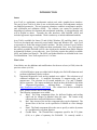
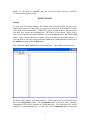
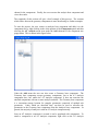
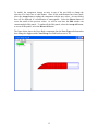
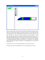
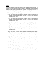
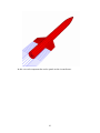
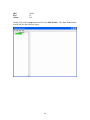
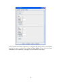
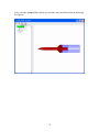
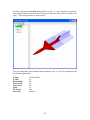
Once started, the Aero Troll window will be displayed. This window is shown below.
At the top of the window is the main menu bar. Below and to the left of the main menu
bar is the Components panel. The Components panel is the area where geometry
components will be shown as nodes in a hierarchical tree. The hierarchical tree will be
referred to as the component tree. To the right of the Components panel is the main
7
display panel. The width of the Components panel and main display panel can be
adjusted by selecting the divider, which separates the two panels, and moving the divider
left or right.
Main Menu Bar
To save an Aero Troll session, select the Save As..., or Save menu item under the File
menu. The Aero Troll session file will be saved as an ASCII XML file. To open a
session file, select the Open menu item under the File menu. If a model already exists in
Aero Troll, the newly opened model will be appended to the existing model.
To quit Aero Troll, select the Quit menu item under the File menu. After the Quit menu
item is selected, a dialog box will appear which asks for confirmation of the action. If the
action is confirmed, Aero Troll will quit immediately. It is up to the user to save any
work before Aero Troll is exited. Quitting Aero Troll will not automatically save the
current session.
Currently Aero Troll does not have the capability to print out a model.
Next to the File menu is the Edit menu. The Edit menu allows the user to cut and copy
components by selecting a component in the component tree and then selecting the Cut
or Copy menu item. To paste a component, select the node in the component tree under
which the component will be pasted and select the Paste menu item. If the component to
be pasted is not allowed under the selected node, the Paste menu item will disabled. The
Edit menu also allows the user to unselect the auto close check box in all PANAIR
execution windows.
The View menu will be described in a later section.
To view the terms and conditions of the Aero Troll license, select the About menu item
under the Help menu.
Problem Specification
The guiding principle behind the design of Aero Troll is to create an aerodynamic
analysis system based on a component buildup approach which allows a user to quickly
experiment with a variety of geometries and analysis approaches. The goal is to create a
tool which predicts preliminary aerodynamics for a given geometry and to create a tool
which can be used to determine the strengths and weaknesses of analysis methods. An
additional goal for Aero Troll is to run on desktops, laptops, and high end workstations
under a variety of operating systems.
To summarize the usage, the user creates an analysis base component and then populates
the analysis base component with geometry components. Flow conditions and reference
values are then specified for the analysis base component and analysis methods are
8
chosen for the components. Finally, the user executes the analysis base component and
views the results.
The remainder of this section will give a brief example of this process. The sections
which follow discuss the geometry components in more detail and give further examples.
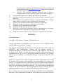
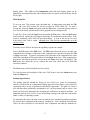
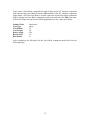
To start the process, the user creates an analysis base component and adds it to the
component tree by right clicking in the white portion of the Components panel and then
selecting the AT Analysis menu item under the Add submenu of the component tree
popup menu. This is shown in the figure below.
Under the Add menu the user can also create a Geometry base component. The
Geometry base component accepts geometry components, just as the AT Analysis
component does, but, unlike the AT Analysis component, it does not associate the
attached components with one or more analysis methods. The Geometry base component
is a convenient storage location for complex geometries comprised of multiple sub
geometries. Links, which are described later, can then be used to reference the
geometries in the Geometry base component from the Analysis base components. In
general, the majority of analysis is with an AT Analysis component only.
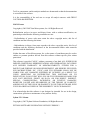
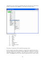
Once an AT Analysis component is created it can be populated with components. To
attach a component to an AT Analysis component, right click on the AT Analysis
9
component tree node to show the component popup menu and select one of the eleven
geometry components from the Add menu. This is shown in the figure below.
The eleven components are:
1)
Nose+Body
2)
Body
3)
Fin Set
4)
Wing
5)
Wedge
6)
Box
7)
Panel
8)
Ground Plane
9)
Field Pts
10)
Coordinate System
11)
Group
The catalog of components will be expanded in upcoming releases.
For this example a Nose+Body component is created with the approach given above.
After the component has been selected from the Add menu, a dialog box will appear
requesting a name for the component. The default can be accepted or a new name
entered. The Rename menu item of the component popup menu can be used to rename
10
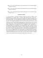
the component at a later time. Once the component is created it will be shown in the
Main Display panel, assuming the AT Analysis component is active (active base
components are described in the Views section below).
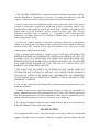
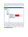
After the component is created, the component parameters can be modified by editing the
component. To edit the component, right click on the Nose+Body component node and
select the Edit menu item in the component popup menu. This is shown below.
11
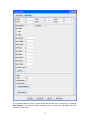
Once the Edit menu item is selected the Edit window with an Edit panel for the
Nose+Body component will be displayed. This is shown below.
12
To modify the component, change an entry in one of the text fields or change the
selection of a check box or radio button. Once all the modifications have been made,
select the Accept button to update the component with the new values. An error dialog
box will be displayed if a modification is unacceptable. Select the Revert button to
revert the entries to the previous values. As will be seen later, the Edit window can
contain multiple Edit panels. To update all the Edit panels, select the Accept All button,
to revert all the panels, select the Revert All button.
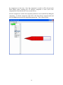
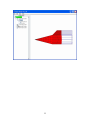
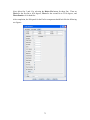
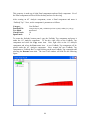
The figure below shows the Nose+Body component after the Nose Type radio button has
been changed to Ogive and the Nose Droop text field has been set to -0.5.
13
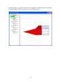
The analysis methodology for the component should be chosen before an analysis is
performed. To select the analysis method for a component, right click on the Nose+Body
component node in the components tree to show the component popup menu and then
select the desired analysis method under the Analysis Type submenu. PANAIR is
chosen in this case.
One of six supersonic/hypersonic local surface analysis methods can also be chosen. The
six local surface analysis methods are comprised of a windward and leeward analysis
method. The selection set of windward methods are: 1) modified Newtonian, 2) tangentwedge, and 3) tangent-cone. The selection set of leeward methods are: 1) p∞ and 2)
Prandtl-Meyer expansion. The impact methods are based on those described in the Mark
IV
Supersonic-Hypersonic
Arbitrary-Body
Computer
Program
(http://handle.dtic.mil/100.2/AD778444). The current set of local surface methods do not
account for shielding.
14
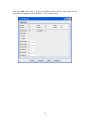
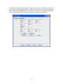
To modify the values associated with an analysis, such as flow conditions and reference
values, open the Analysis Edit panel by right clicking on the AT Analysis component
node and selecting the Edit menu item under the AT Analysis component popup menu.
The AT Analysis Edit panel for the AT Analysis component is shown below.
15
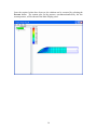
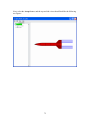
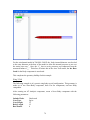
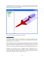
Once the required values have been set, the solution can be executed by selecting the
Execute button. The contour plot for the pressure, non-dimensionalized by the free
stream pressure, will be shown in the Main Display panel.
16
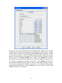
Select the Results button in the AT Analysis Edit panel or the Results menu item in the
AT Analysis component popup menu to view the integrated results, s. The AT Analysis
Results panel, which is contained in the Result window, is shown below.
Views
The base component must be activated to view it in the Main Display panel. Only one
base component can be active at a time. Select the Activate or Deactivate menu item
from the base component popup menu to activate or deactivate the base component.
The Main Display panel allows the user to translate, rotate, and zoom in and out. To
translate the image, hold down the left mouse button and move the mouse in the direction
the image should be translated. To rotate the image, hold down the right mouse button
and move the mouse forward or backward to rotate the image about the x axis of the
screen. Moving the mouse right or left will rotate the image about the y axis of the
screen. To zoom the image, hold down the middle mouse button and move the mouse
forward to zoom out of the image or move the mouse backward to zoom into the image.
The view for the Main Display panel can be reset to one of six predefined views (top,
bottom, right, left, front, and back) by selecting the view from the View menu located in
the main menu bar.
17
Checking PANAIR Abutments
An important step in the creation of a PANAIR solution is the inspection of the network
edge abutments. Each network has four edges and each edge has a top and bottom side.
Each side of the four edges of a panel network must do one of the following: 1) connect
to an edge side of this or another network, 2) connect to the opposite side of this edge, or
3) coalesce into a single point. In addition, each side of an edge is either an internal or
external type, depending on whether it is on the inside or outside of the geometry. An
edge side can only connect to another side of the same type. So, an internal side must
connect to an internal side and an external side must connect to an external side. If an
edge side incorrectly connects to another edge side or remains unconnected then the
solution from PANAIR will be erroneous.
To check the PANAIR network abutments, right click on the AT Analysis component
node in the example of the prior section and select the Check PANAIR menu item.
Aero Troll will do a rudimentary automatic check and will present a message dialog for
any errors encountered. To perform a manual investigation of the PANAIR networks and
abutments, first the PANAIR networks and abutments must be displayed and the
geometry components hidden. To show the PANAIR networks and abutments, right
click on the AT Analysis component and select the Show PANAIR menu item in the
component popup menu, as seen below.
18
Since the PANAIR networks and abutments overlay the geometry components, the
geometry components need to be hidden. To hide the geometry components, right click
on the AT Analysis component and select the Hide All menu item in the component
popup menu.
19
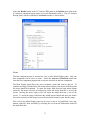
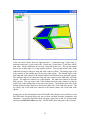
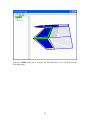
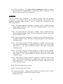
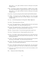
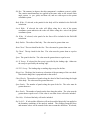
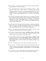
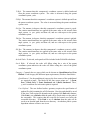
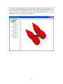
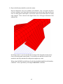
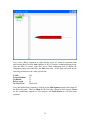
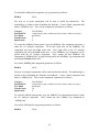
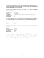
Once the geometry components are hidden, the Aero Troll window will look like the
image below.
20
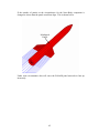
The various networks are shown in blue with a black or blue border in the figure above.
In this case, there are four networks: nose, body, base, and wake. The surface networks
(nose, body, and base) have a black border and the surface is colored in with blue. The
wake networks have a blue border and the wireframe of the wake network is colored
blue. The edge of the network is colored according to the type of abutment. A green
abutment indicates that the side of an edge has successfully connected to another edge. A
yellow abutment indicates that the side of an edge has either connected to the other side
of that edge or that the side belongs to a trailing edge of a wake which extends to infinity.
A clear abutment indicates that the edge coalesces to a single point. A red abutment
indicates that either the edge has connected to an incompatible edge or that it has not
connected at all.
It is up to the end user to ensure that the abutments are connected as expected.
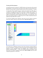
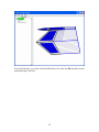
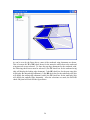
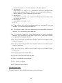
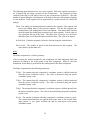
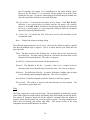
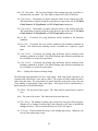
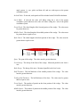
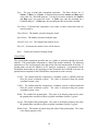
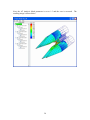
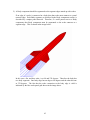
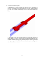
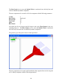
The figure below shows the PANAIR check view of a tank attached to a wing tip.
21
In the case shown above there are eight networks: 1) starboard wing, 2) port wing, 3)
starboard wing wake, 4) port wing wake, 5) tank nose, 6) tank body, 7) tank base, and 8)
tank wake. All the abutments are correctly connected in this case. The top and bottom
sides of the leading edge of a wing connect (yellow). The top and bottom sides of the
outboard (tip) edges of the port wing and wake connect (yellow). The trailing edge of the
wing connects to the leading edge of the wing wake (green). The inboard edges of the
port wing and wake connect to the inboard edges of the starboard wing and wake (green).
The outboard edge of the starboard wing and wake connect to the tank body and wake
(green). The tank nose coalesces to a point (blank). The tank nose connects to the tank
body (green). The top (outer) side of the trailing tank body edge connects to the top
(outer) side of the leading edge of the tank wake (green). The bottom (inner) side of the
trailing tank body edge connects to the bottom (inner) side of the tank base (green). The
top (outer) side of the tank base connects to the bottom (inner) side of the tank wake
(green).
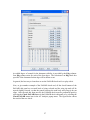
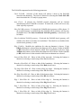
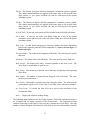
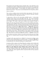
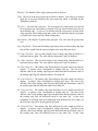
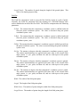
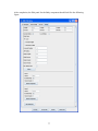
Seeing some of this information from the PANAIR check display can be difficult, so the
PANAIR check edit panel allows the user to show and hide networks, boundaries, and
abutments. To open the PANAIR check edit panel, right click on the AT Analysis node
and select the Edit PANAIR menu item. The PANAIR check edit panel is shown below.
22
The primary area of the PANAIR edit panel for modifying the visibility of the networks
and abutments is the table of check buttons located at the bottom of the window. The Net
column controls the visibility of the networks and the Bndr column controls the visibility
of the network boundary. The TE and BE columns determine whether the top and
bottom side of an abutment will be displayed. The behavior of these columns is affected
by the selection of the Edge Visibility radio buttons. If the ORed radio button is
selected then the abutment will be shown if one of the TE (or BE) check boxes for the
two networks comprising the abutment are selected. If the ANDed radio button is
selected, then the abutment will be shown if both of the TE (or BE) check boxes for the
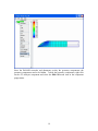
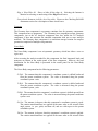
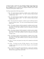
two networks comprising the abutment are selected. For example, the figure below
shows the PANAIR check view when the ORed radio button is selected and all the TE
and BE check boxes are unselected.
23
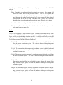
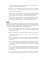
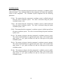
Next, the following view shows the PANAIR check view after the BE checkbox for the
starboard wing is selected.
24
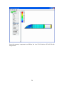
After the ANDed radio box is selected, the PANAIR check view will look like the
following image.
25
As can be seen by the figure above, none of the starboard wing abutments are shown.
This is because the TE or BE check boxes for the networks which abut to the starboard
wing network are not selected. To show the top edge abutments for the starboard wind,
the following check boxes must be selected: 1) the TE check box for the starboard wing
(this will display the leading edge abutment), 2) the BE check box for the port wing (this
will display the inboard edge abutment), 3) the BE check box for the starboard wake (this
will display the trailing edge abutment), and 4) the TE check box for the tank body (this
will display the outboard edge abutment). After the selections are made, the PANAIR
check edit panel will look like the figure below.
26
An added degree of control for the abutment visibility is provided by the Edg columns.
One Edg column exists for each of the four edges. The selection of an Edg check box
specifies if the abutment for that edge will be shown or not.
In general, the best way to learn how to use the PANAIR check tool is to play with it.
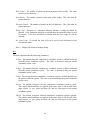
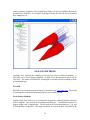
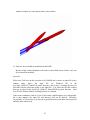
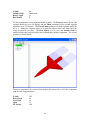
Now, to give another example of the PANAIR check tool, all the check buttons of the
PANAIR edit panel are reverted back to being selected and the wing tip tank will be
moved slightly forward, so that the panels between the tank body and wing tip do not
align. After the tank has been moved, the PANAIR check must be performed again by
selecting the Check PANAIR button in the PANAIR check edit panel or by selecting the
Check PANAIR menu item in the AT Analysis popup menu. The figure below shows
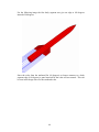
the result of the new check.
27
As can be seen from the figure above, after the shift, the starboard wing tip does not abut
with the tank body anymore; instead the starboard wing tip connects with itself. This will
create an erroneous result.
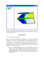
COMPONENTS
This section describes each component.
Some of the components below allow for specification of how a wake interacts with
components. This is done through advanced settings. The advanced settings for a
component can be accessed by selecting the More... button located in the edit panel for
that component. If a component supports these advanced settings, it will be mentioned in
the descriptions below. The current two advanced settings are described below. The
Accept button in the edit panel for a component must be selected after the advanced
setting for that component is changed.
Sticky Wakes: If the Sticky Wakes check box is selected and the inboard or outboard
edge of a wake from the component associated with the checkbox touches a
network edge of another component, then Aero Troll will attach the wake to that
network edge and the wake will follow along the length of that network edge. If
the Sticky Wakes check box is not selected, then the wake will not attach to the
network edge.
28
Reject Wake Attachments: If the Reject Wake Attachments checkbox is selected,
then the inboard or outboard edge of a wake from another component will not
attach to a network edge of this component.
AT Analysis
The AT Analysis base component is an analysis container class for geometry
components. As an analysis class it allows for the organization and execution of the
geometry component analysis methods. The AT Analysis base component has the
following parameters.
X Shift: The amount that this component’s coordinate system is shifted backward
from the global coordinate system. The value is measured along the x axis of the
global coordinate system.
Y Shift: The amount that this component’s coordinate system is shifted starboard
from the global coordinate system. The value is measured along the y axis of the
global coordinate system.
Z Shift: The amount that this component’s coordinate system is shifted upward from
the global coordinate system. The value is measured along the z axis of the global
coordinate system.
Psi Rot: The amount, in degrees, that this component’s coordinate system is yawed.
The rotation transformations are applied in the same order as the aircraft Euler
angle system, i.e. yaw, pitch, and then roll, and are with respect to the global
coordinate system.
Tht Rot: The amount, in degrees, that this component’s coordinate system is pitched.
The rotation transformations are applied in the same order as the aircraft Euler
angle system, i.e. yaw, pitch, and then roll, and are with respect to the global
coordinate system.
Phi Rot: The amount, in degrees, that this component’s coordinate system is rolled
about. The rotation transformations are applied in the same order as the aircraft
Euler angle system, i.e. yaw, pitch, and then roll, and are with respect to the
global coordinate system.
Mach: The Mach number for the analysis.
Gamma: The ratio of the specific heats.
Flow Angle Specification: The drop down selection box allows the user to choose
one of five methods to enter the free stream flow angle.
1) alphac-phi (αc, φ)
29
2)
3)
4)
5)
where u=V∞*cos(αc), v=-V∞*sin(αc)*sin(φ), w=V∞*sin(αc)*cos(φ) .
sin-sin (αs, βs)
where sin(αs)=w/V∞, sin(βs)=-v/V∞. Note that the u velocity is ambiguous when
both αs and βs are greater than 90. Therefore it is assumed in this formulation
that the intent of βs is to be in the range of ±90 degrees.
tan-tan (αt, βt)
where tan(αt)=w/u, tan(βt)=-v/u. This form is indeterminate when both αt and βt
are equal to ±90 degrees.
tan-sin (αt, βs)
where tan(αt)=w/u, sin(βs)==-v/V∞.
u, v, w
sRef: The reference area used to non-dimensionalize the aerodynamic forces and
moments. The value must be greater than zero.
lRef: The reference length used to non-dimensionalize the longitudinal aerodynamic
moments. The value must be greater than zero.
bRef: The reference length used to non-dimensionalize the lateral aerodynamic
moments. The value must be greater than or equal to zero. If the value is equal to
zero then lRef will substitute for bRef.
xMom: The x value for the moment center measured in the local coordinate system.
Positive is rearward.
yMom: The y value for the moment center measured in the local coordinate system.
Positive is starboard.
zMom: The z value for the moment center measured in the local coordinate system.
Positive is up.
Check PANAIR: Execute PANAIR check.
Edit PANAIR: Open PANAIR check edit panel.
Invalidate: Invalidate the current solution.
Execute: Execute a solution.
Results: Show the results window.
PANAIR Helper Agent
The general usage for the PANAIR helper agent was described above.
30
The PANAIR component has the following parameters.
Check PANAIR: Selection of this button will initiate a check of the PANAIR
networks and abutments. The action is identical to selecting the Check PANAIR
menu item under the AT Analysis popup menu.
Auto Check: If selected, the PANAIR network abutments will be checked
automatically before PANAIR is executed. If unselected, a check will occur only
when explicitly requested.
Show PANAIR geometry: If selected, the PANAIR check geometry will be shown. If
the overall geometry is modified then the PANAIR check geometry will become
invalidated and, if the Show Invalidated PANAIR geometry is unselected, will
be hidden.
Show Invalidated PANAIR geometry: If selected, the PANAIR check geometry will
continue to be shown even after it is invalidated. This check box is disabled if the
current check geometry is valid.
Edge Visibility: Modifies the conditions for when an abutment is shown. If the
ORed radio button is selected then the abutment will be shown if either of the TE
(or BE) check boxes for the networks which form an abutment is selected. If the
ANDed radio button is selected then the abutment will be shown if both of the TE
(or BE) check boxes for the networks which form an abutment are selected.
Network Show/Hide All: Show or hide all the networks. Selecting the buttons is
identical to selecting or unselecting all the Net check boxes.
Boundary Show/Hide All: Show or hide all the boundaries. Selecting the buttons is
identical to selecting or unselecting all the Bndr check boxes.
Top Edge Show/Hide All: Show or hide all the top edges. Selecting the buttons is
identical to selecting or unselecting all the TE check boxes.
Bot Edge Show/Hide All: Show or hide all the bottom edges. Selecting the buttons is
identical to selecting or unselecting all the BE check boxes.
Edge 1 Show/Hide All: Show or hide all the edge 1s. Selecting the buttons is
identical to selecting or unselecting all the Edg1 check boxes.
Edge 2 Show/Hide All: Show or hide all the edge 2s. Selecting the buttons is
identical to selecting or unselecting all the Edg2 check boxes.
Edge 3 Show/Hide All: Show or hide all the edge 3s. Selecting the buttons is
identical to selecting or unselecting all the Edg3 check boxes.
31
Edge 4 Show/Hide All: Show or hide all the edge 4s. Selecting the buttons is
identical to selecting or unselecting all the Edg4 check boxes.
Network and Abutment visibility check box table: Please see the Checking PANAIR
Abutments section for a description of these check boxes.
Geometry
The Geometry base component is a geometry container class for geometry components.
This component has no parameters. The Geometry base component accepts geometry
components, just as the AT Analysis component does, but, unlike the AT Analysis
component, it does not associate the attached components with one or more analysis
methods. The Geometry base component is a convenient storage location for complex
geometries comprised of multiple sub geometries.
Nose+Body
The Nose+Body component is an axisymmetric geometry which has either a cone or
ogive nose.
After executing the analysis method for this component, the final integrated loads and
moments are shown in the results panel of the base component. However, the load
distribution for the Nose+Body is presented in the results panel for the Nose+Body
component.
The Nose+Body component has the following parameters.
X Shift: The amount that this component’s coordinate system is shifted backward
from the parent coordinate system. The value is measured along the parent
coordinate system x axis.
Y Shift: The amount that this component’s coordinate system is shifted starboard
from the parent coordinate system. The value is measured along the parent
coordinate system y axis.
Z Shift: The amount that this component’s coordinate system is shifted upward from
the parent coordinate system. The value is measured along the parent coordinate
system z axis.
Psi Rot: The amount, in degrees, that this component’s coordinate system is yawed.
The rotation transformations are applied in the same order as the aircraft Euler
angle system, i.e. yaw, pitch, and then roll, and are with respect to the parent
coordinate system.
Tht Rot: The amount, in degrees, that this component’s coordinate system is pitched.
The rotation transformations are applied in the same order as the aircraft Euler
32
angle system, i.e. yaw, pitch, and then roll, and are with respect to the parent
coordinate system.
Phi Rot: The amount, in degrees, that this component’s coordinate system is rolled.
The rotation transformations are applied in the same order as the aircraft Euler
angle system, i.e. yaw, pitch, and then roll, and are with respect to the parent
coordinate system.
Include Wake: If selected, wake panels will be included in the PANAIR calculation.
Local Wake: If selected, the wake will follow along the x axis of the parent
coordinate system otherwise the wake will follow along the x axis of the global
coordinate system.
Nose Type: A radio button grouping for selecting either a Cone or Ogive nose.
Nose Radius: The maximum radius of the nose.
Nose Length: The length of the nose. Measured parallel to the local x axis from the
nose tip to the shoulder. This value must be greater than zero.
Body Length: The length of the body. Measured parallel to the local x axis from the
shoulder to the base. The value must be greater than or equal to zero.
Tip Radius: The nose tip radius. The value must be greater than or equal to zero.
Nose Droop: The droop of the nose. Measured parallel to the local z axis.
Tip Panels: The number of panels laid out along the nose tip center line from the
forward point of the nose tip to the junction of the nose tip and nose. The value
must be greater than zero.
Nose Panels: The number of panels laid out in the axial direction from the junction
of the nose tip to the shoulder. The value must be greater than zero.
Body Panels: The number of panels laid out in the axial direction from the shoulder
to the base. The value must be greater than zero.
Base Panels: The number of panels on the base along the radius. The value must be
greater than or equal to zero. If the value is zero then a base will not be included.
Inc. Base Load: If selected the base will not be used in the calculation of the
aerodynamic loads.
More...: Display the advanced settings dialog.
33
The following input parameters are for a nose segment. Each nose segment represents a
set of panels laid out along a portion of the circumference. The segments are then
connected side edge to side edge to loop over the circumference of the nose. The total
number of panels along the circumference of the body is the sum of the number of panels
in each segment. Each segment will be represented by a panel network for a PANAIR
analysis.
Theta: The ending circumferential theta location for the segment. The segment will
start at the ending theta of the previous segment. For the first segment, the
starting theta is the ending theta of the last segment. The ending theta location
must not match the ending theta location of any other segment. A theta value of
zero represents the top of the body. The theta value is positive in a clockwise
direction when viewed from the back towards the front. The value is in degrees.
Include Body: If unselected panels will not be laid out along the circumference.
Theta Panels: The number of panels in the theta direction for this segment. The
value must be greater than zero.
Body
The Body component is a circular geometry.
After executing the analysis method for this component, the final integrated loads and
moments are shown in the results panel of the base component. However, the load
distribution for the Body is presented in the results panel for the Body component.
The Body component has the following parameters.
X Shift: The amount that this component’s coordinate system is shifted backward
from the parent coordinate system. The value is measured along the parent
coordinate system x axis.
Y Shift: The amount that this component’s coordinate system is shifted starboard
from the parent coordinate system. The value is measured along the parent
coordinate system y axis.
Z Shift: The amount that this component’s coordinate system is shifted upward from
the parent coordinate system. The value is measured along the parent coordinate
system z axis.
Psi Rot: The amount, in degrees, that this component’s coordinate system is yawed.
The rotation transformations are applied in the same order as the aircraft Euler
angle system, i.e. yaw, pitch, and then roll, and are with respect to the parent
coordinate system.
34
Tht Rot: The amount, in degrees, that this component’s coordinate system is pitched.
The rotation transformations are applied in the same order as the aircraft Euler
angle system, i.e. yaw, pitch, and then roll, and are with respect to the parent
coordinate system.
Phi Rot: The amount, in degrees, that this component’s coordinate system is rolled.
The rotation transformations are applied in the same order as the aircraft Euler
angle system, i.e. yaw, pitch, and then roll, and are with respect to the parent
coordinate system.
Include Wake: If selected, wake panels will be included in the PANAIR calculation.
Local Wake: If selected, the wake will follow along the x axis of the parent
coordinate system otherwise the wake will follow along the x axis of the global
coordinate system.
Body Type: A radio button grouping for selecting whether the radius distribution
between the beginning and end of this component is a Cone, Forward Ogive, or
Backward Ogive.
Forward Radius: The radius at the beginning of the body. The value must be greater
than zero.
Aft Radius: The radius at the end of the body. The value must be greater than zero.
Body Length: The length of the body. Measured parallel to the local x axis. The
value must be greater than or equal to zero.
Body Droop: The amount by which the end of the body is higher than the beginning
of the body.
Body Panels: The number of panels laid out along the axis of the body. The value
must be greater than zero.
Base Panels: The number of panels on the base along the radius. The value must be
greater than or equal to zero. If the value is zero then a base will not be included.
Inc. Base Load: If selected the base will not be used in the calculation of the
aerodynamic loads.
More...: Display the advanced settings dialog.
The following input parameters are for a body segment. Each body segment represents a
set of panels laid out along a portion of the circumference. The segments are then
connected side edge to side edge to loop over the circumference of the body. The total
number of panels along the circumference of the body is the sum of the number of panels
35
in each segment. Each segment will be represented by a panel network for a PANAIR
analysis.
Theta: The ending circumferential theta location for the segment. The segment will
start at the ending theta of the previous segment. For the first segment, the
starting theta is the ending theta of the last segment. The ending theta location
must not match the ending theta location of any other segment. A theta value of
zero represents the top of the body. The theta value is positive in a clockwise
direction when viewed from the back towards the front. The value is in degrees.
Include Body: If unselected panels will not be laid out along the circumference.
Theta Panels: The number of panels in the theta direction for this segment. The
value must be greater than zero.
Fin Set
The Fin Set component is used to model fin sets. Each fin in the fin set has the same
planform shape. The fin planforms are modeled with straight leading edge and trailing
edges, and the root chord and tip chord are parallel. It is possible to deflect the entire fin
set but currently tailing edge flaps, leading edge flaps, and ailerons can not be specified.
The Fin Set component has the following parameters.
X Shift: The amount that this component’s coordinate system is shifted backward
from the parent coordinate system. The value is measured along the parent
coordinate system x axis.
Y Shift: The amount that this component’s coordinate system is shifted starboard
from the parent coordinate system. The value is measured along the parent
coordinate system y axis.
Z Shift: The amount that this component’s coordinate system is shifted upward from
the parent coordinate system. The value is measured along the parent coordinate
system z axis.
Psi Rot: The amount, in degrees, that this component’s coordinate system is yawed.
The rotation transformations are applied in the same order as the aircraft Euler
angle system, i.e. yaw, pitch, and then roll, and are with respect to the parent
coordinate system.
Tht Rot: The amount, in degrees, that this component’s coordinate system is pitched.
The rotation transformations are applied in the same order as the aircraft Euler
angle system, i.e. yaw, pitch, and then roll, and are with respect to the parent
coordinate system.
36
Phi Rot: The amount, in degrees, that this component’s coordinate system is rolled.
The rotation transformations are applied in the same order as the aircraft Euler
angle system, i.e. yaw, pitch, and then roll, and are with respect to the parent
coordinate system.
Body Wake: If selected, wake panels for the body will be included in the PANAIR
calculation.
Local Wake: If selected, the wake will follow along the x axis of the parent
coordinate system otherwise the wake will follow along the x axis of the global
coordinate system.
Fin Wake: If selected, wake panels for the fins will be included in the PANAIR
calculation.
Body Radius: The radius of the body. The value must be greater than zero.
Root Chord: The root chord for the fins. The value must be greater than zero.
Tip Chord: The tip chord for the fins. The value must be greater than or equal to
zero.
Span: The span for the fins. The value must be greater than or equal to zero.
Is L.E. Sweep: If selected, the fin sweep is specified by the leading edge. Otherwise
the sweep is specified by the trailing edge.
L.E./T.E. Sweep: The leading edge or trailing edge sweep for the fins.
Hinge Line: The hinge line location as a function of the percentage of the root chord.
Note that the hinge line is perpendicular to the surface.
Chord Panels: The number of panels along the chord of the fin and along the length
of the body. The value must be greater than zero.
Span Panels: The number of panels along the span of the fin. The value must be
greater than zero.
Base Panels: The number of panels on the base along the radius. The value must be
greater than or equal to zero. If the value is zero then a base will not be included.
Fins Only: If selected the body will not be included.
Def. In B.C.: If selected the deflection will not be modeled physically but applied to
the boundary conditions of the analysis method. The resulting integrated force
and moment values will be rotated to take into account the deflection. If selected,
37
the fin paneling will appear to be undeflected in the Main Display panel.
However the fin outline, if it is activated, will be deflected to provide visual
feedback to the user. In general, when using the PANAIR analysis method, this
check box should be selected for cases with deflection.
Show fin outlines: If selected the fin outline will be shown. If the Def. In B.C.
checkbox is not selected then fin outline and the fin panels will coincide.
However, if the Def. In B.C. checkbox is selected then fin outline will represent
the fin as it would appear if it were physically deflected while the fin panels
represent a physically undeflected fin.
Inc. Base Load: If selected the base will not be used in the calculation of the
aerodynamic loads.
More...: Display the advanced settings dialog.
The following input parameters are for a fin. Note that the deflection angle is applied
first then the dihedral angle is applied. This is to insure that the root chord does not
pierce the body.
Theta: The theta location of the fin hinge line. A theta value of zero represents the
top of the body. The theta value is positive in a clockwise direction when viewed
from the back towards the front. The value is in degrees.
Include Fin: If unselected, this section will not include a fin.
Dihedral: The dihedral of the fin. A positive value is in a counter clockwise
direction when viewed from the back towards the front. The value is in degrees.
Deflection: The deflection of the fin. A positive deflection is leading edge up when
viewed looking outward along the hinge line. The value is in degrees.
Include Body: If unselected panels will not be laid out on the body segment.
Theta Panels: The number of panels in the theta direction for this segment. The
value must be greater than zero.
Wing
The Wing component is used to model wings. The wing planform is modeled by regions
where each region has straight leading and trailing edges and straight root and tip chords.
The number of chordwise panels for all the regions is constant whiles the number of
spanwise panels for the regions can vary from region to region. The wing component can
model twist and leading and trailing edge flaps. The current version of the wing
component does not model thickness or camber.
38
Each wing has a true and paneled geometry associated with it. If any deflection or twist
is modeled in the boundary condition then the deflection and twisted will be incorporated
in the physical geometry layout of the true geometry and will not be incorporated in the
layout of the paneled geometry. For the analysis, the paneled geometry is used to
determine the pressures. The pressures are then transferred to the true geometry and the
loads are calculated.
There are three coordinate systems associated with the wing component. The first is the
wing component coordinate system, the second is the deflected wing hinge coordinate
system, and the third is the wing region root system.
A wing region is laid out in the wing region coordinate system. A wing region
coordinate system exists for every wing region of the wing. The x axis of wing region
coordinate system is aligned with the root chord of the wing region. The z axis of the
wing region coordinate system is parallel to the normal vector of the wing region before
twist is applied. The origin of wing region coordinate system depends on whether it
belongs to the first wing region (the inboard one) or one of the remaining wing regions.
If the wing region coordinate system is for the first wing region then the origin is located
at the hinge point of the wing. The hinge point of the wing is located on the wing root
chord and is a fraction of the root chord rearward from the wing root chord leading edge.
This fraction is specified by the Hinge Line parameter. A Hinge Line value of 0.0
indicates that the hinge point is located at the root chord leading edge and a Hinge Line
value of 1.0 indicates that the hinge point is located at the root chord trailing edge. If the
wing region is one of the remaining wing regions then the origin is located at the twist
point of the previous region. The twist point of a wing region is located on the wing
region tip chord and is a fraction of the tip chord rearward from the tip chord leading
edge. This fraction is specified by the Twist Loc. parameter. A Twist Loc. value of 0.0
indicates that the twist point is located at the region tip chord leading edge and a Twist
Loc. value of 1.0 indicates that the twist point is located at the region tip chord trailing
edge.
Assuming the first wing region has zero dihedral, the wing region coordinate system
coincides with the deflected hinge line coordinate system. The parameter Dihedral of
the first wing region specifies the amount the x axis of the wing region coordinate system
is rolled about the x axis of the deflected hinge line coordinate system.
Assuming no shifts or rotations, the deflected hinge line coordinate system coincides with
the wing component coordinate system. The wing hinge coordinate system is shifted and
rotated from the wing component coordinate system by amounts specified by the Y Shift,
Hinge Yaw Angle, Hinge Cant Angle, Incidence Angle, and Def. Angle parameters.
First the incidence and deflection angle are applied to pitch the wing. Then the hinge
cant angle is applied to roll the wing. Then the hinge yaw angle is applied to yaw the
wing. Finally, the y shift is applied to shift the wing outward from the wing component
coordinate system.
39
Assuming no shifts or rotations, the wing component coordinate system coincides with
the parent coordinate system. The parameters X Shift, Y Shift, Z Shift, Psi Rot, Tht
Rot, and Phi Rot specify the amount the wing component coordinate system is shifted
and rotated from the parent coordinate system
The Wing component has the following parameters.
X Shift: The amount that this component’s coordinate system is shifted backward
from the parent coordinate system. The value is measured along the parent
coordinate system x axis.
Y Shift: The amount that this component’s coordinate system is shifted starboard
from the parent coordinate system. The value is measured along the parent
coordinate system y axis.
Z Shift: The amount that this component’s coordinate system is shifted upward from
the parent coordinate system. The value is measured along the parent coordinate
system z axis.
Psi Rot: The amount, in degrees, that this component’s coordinate system is yawed.
The rotation transformations are applied in the same order as the aircraft Euler
angle system, i.e. yaw, pitch, and then roll, and are with respect to the parent
coordinate system.
Tht Rot: The amount, in degrees, that this component’s coordinate system is pitched.
The rotation transformations are applied in the same order as the aircraft Euler
angle system, i.e. yaw, pitch, and then roll, and are with respect to the parent
coordinate system.
Phi Rot: The amount, in degrees, that this component’s coordinate system is rolled.
The rotation transformations are applied in the same order as the aircraft Euler
angle system, i.e. yaw, pitch, and then roll, and are with respect to the parent
coordinate system.
Body Wake: If selected, wake panels for the body will be included in the PANAIR
calculation.
Local Wake: If selected, the wake will follow along the x axis of the parent
coordinate system otherwise the wake will follow along the x axis of the global
coordinate system.
Reflect: If selected the wing will be mirrored about the x-z plane of the component.
Well, mostly. If a leading or trailing edge has any roll deflection, then that
deflection will be opposite on the mirrored side.
40
Show wing outlines: If selected, an outline of the true geometry of the wing will be
shown in addition to the paneled geometry.
Y Shift: The amount that the wing hinge point (see Hinge Line below) is shifted
starboard from the wing x-z plane. The value is measured along the wing
component coordinate system y axis. The hinge point transformations are done in
the following order: 1) The Hinge Cant Angle, 2) The Hinge Yaw Angle, and 3)
Y Shift. The hinge point transformations do not effect the wing coordinate
system.
Hinge Yaw Angle: The amount, in degrees, that the wing is yawed about a line which
passes through the hinge point and is parallel to the wing component coordinate
system z axis. Positive values rotate the wing tip forward. The hinge point
transformations are done in the following order: 1) The Hinge Cant Angle, 2)
The Hinge Yaw Angle, and 3) Y Shift. The hinge point transformations do not
effect the wing coordinate system.
Hinge Cant Angle: The amount, in degrees, that the wing is canted up (wing tip up)
about the root chord. The hinge point transformations are done in the following
order: 1) The Hinge Cant Angle, 2) The Hinge Yaw Angle, and 3) Y Shift. The
hinge point transformations do not effect the wing coordinate system.
Hinge Line: The location of the hinge point (origin of hinge line coordinate system)
along the root chord measured as a fraction of the root chord.
Incidence Angle: Incidence angle of the wing. The Incidence Angle and Def. Angle
parameters have the same effect if the Def. In B.C. checkbox is unselected. The
incidence angle is always modeled as a physical parameter.
Def. Angle: Deflection angle of the wing. The Def. Angle and Incidence Angle
parameters have the same effect if the Def. In B.C. checkbox is unselected. If the
Def. In B.C. checkbox is unselected the deflection angle will be modeled as a
physical angle otherwise it will be modeled in the boundary condition of the
analysis method.
Root Chord: The length of the root chord. Must be greater than or equal to zero.
Main Chord Panels: The number of panels along the chord between the leading and
trailing edge flaps. The total number of panels along the wing chord is equal to
the sum of the Main Chord Panels, L.E. Flap Panels, and T.E. Flap Panels
parameters.
Root L.E. Flap Ratio: The root chord length of the leading edge flap specified as a
fraction of the root chord. The value must be between 0.0 and 1.0 inclusive.
41
Root T.E. Flap Ratio: The root chord length of the trailing edge flap specified as a
fraction of the root chord. The value must be between 0.0 and 1.0 inclusive.
L.E. Flap Panels: The number of panels along the chord of the leading edge flap.
The total number of panels along the wing chord is equal to the sum of the Main
Chord Panels, L.E. Flap Panels, and T.E. Flap Panels parameters.
T.E. Flap Panels: The number of panels along the chord of the trailing edge flap.
The total number of panels along the wing chord is equal to the sum of the Main
Chord Panels, L.E. Flap Panels, and T.E. Flap Panels parameters.
Def. In B.C.: If selected, the wing deflection will be modeled in the boundary
condition.
Twist In B.C.: If selected, the twist will be modeled in the boundary condition by
default. The default twist modeling can be overridden on a region by region
basis.
L.E. Def. In B.C.: If selected, the leading edge deflection will be modeled in the
boundary condition by default. The default leading edge deflection modeling can
be overridden on a region by region basis.
T.E. Def. In B.C.: If selected, the trailing edge deflection will be modeled in the
boundary condition by default. The default leading edge deflection modeling can
be overridden on a region by region basis.
More...: Display the advanced settings dialog.
The following input parameters are for a wing region. Each wing region represents a set
of panels laid out between a root and tip chord. The regions are then connected end to
end to form the wing. The total number of panels along the span of the wing is the sum
of the number of span panels along each region. Each region will be represented by a
panel network for a PANAIR analysis.
Tip Chord: The tip chord of the region. The value must be greater than or equal to
zero.
Span: The span of the region. The value must be greater than zero.
L.E./T.E. Sweep: The leading or tailing edge sweep of the wing specified in degrees.
Whether it is a leading or trailing edge value depends on the state of the Is L.E.
Sweep check box. The sweep must be between 90 and -90 degrees.
Is L.E. Sweep: If selected then the sweep is the leading edge sweep. Otherwise, the
sweep is the trailing edge sweep.
42
Dihedral: The dihedral of the wing region specified in degrees.
Twist: The twist of the wing region tip specified in degrees. The wing tip is rotated
about the twist point located on the wing region tip which is specified by the
Twist Loc. parameter.
Twist Loc.: Specified the twist point. The twist point of a wing region is located on
the wing region tip chord and is a fraction of the tip chord rearward from the tip
chord leading edge. A value of 0.0 indicates that the twist point is located at the
wing region tip chord leading edge and a value of 1.0 indicates that the twist point
is located at the wing region tip chord trailing edge.
Span Panels: The number of panels along the span. The value must be greater than
zero.
Copy Flap Ratios: If selected the leading edge flap tip ratio and the trailing edge flap
ratio will be copied from the previous region or the wing flap root ratios.
L.E. Flap Tip Ratio: The tip chord length of the leading edge flap specified as a
fraction of the tip chord. The value must be between 0.0 and 1.0 inclusive.
T.E. Flap Tip Ratio: The tip chord length of the trailing edge flap specified as a
fraction of the tip chord. The value must be between 0.0 and 1.0 inclusive.
L.E. Flap Pitch Def: The leading edge flap deflection for pitch control specified in
degrees. A positive value corresponds to leading edge up. The sum of the
absolute value of the leading edge flap pitch deflection and the absolute value of
the leading edge flap roll deflection must be less than 180.
T.E. Flap Pitch Def: The trailing edge flap deflection for pitch control specified in
degrees. A positive value corresponds to trailing edge down. The sum of the
absolute value of the trailing edge flap pitch deflection and the absolute value of
the trailing edge flap roll deflection must be less than 180.
L.E. Flap Roll Def: The leading edge flap deflection for roll control specified in
degrees. A positive value corresponds to leading edge up. The sum of the
absolute value of the leading edge flap pitch deflection and the absolute value of
the leading edge flap roll deflection must be less than 180. If this wing
component is reflected, then the leading edge flap deflection for roll control on
the reflected wing will be in the opposite direction.
T.E. Flap Roll Def: The tailing edge flap deflection for roll control specified in
degrees. A positive value corresponds to tailing edge down. The sum of the
absolute value of the trailing edge flap pitch deflection and the absolute value of
the trailing edge flap roll deflection must be less than 180. If this wing
43
component is reflected, then the trailing edge flap deflection for roll control on the
reflected wing will be in the opposite direction.
Twist in B.C.: A set of radio buttons to determine how the twist will be modeled.
The choices are to: 1) use the setting from the wing, 2) model twist in boundary
condition, 3) model twist physically.
L.E. Def. In B.C.: A set of radio buttons to determine how the leading edge deflection
will be modeled. The choices are to: 1) use the setting from the wing, 2) model
the deflection in boundary condition, or 3) model the deflection physically.
T.E. Def. In B.C.: A set of radio buttons to determine how the leading edge deflection
will be modeled. The choices are to: 1) use the setting from the wing, 2) model
the deflection in boundary condition, or 3) model the deflection physically.
Wedge
Currently the intent of the Wedge component is to use it as an independent component
which is not physically connected to the Nose+Body, Body, or Fin Set components. The
origin or the component coordinate system is located halfway along the span of the
leading edge. The Wedge component has the following parameters.
X Shift: The amount that this component’s coordinate system is shifted backward
from the parent coordinate system. The value is measured along the parent
coordinate system x axis.
Y Shift: The amount that this component’s coordinate system is shifted starboard
from the parent coordinate system. The value is measured along the parent
coordinate system y axis.
Z Shift: The amount that this component’s coordinate system is shifted upward from
the parent coordinate system. The value is measured along the parent coordinate
system z axis.
Psi Rot: The amount, in degrees, that this component’s coordinate system is yawed.
The rotation transformations are applied in the same order as the aircraft Euler
angle system, i.e. yaw, pitch, and then roll, and are with respect to the parent
coordinate system.
Tht Rot: The amount, in degrees, that this component’s coordinate system is pitched.
The rotation transformations are applied in the same order as the aircraft Euler
angle system, i.e. yaw, pitch, and then roll, and are with respect to the parent
coordinate system.
Phi Rot: The amount, in degrees, that this component’s coordinate system is rolled.
The rotation transformations are applied in the same order as the aircraft Euler
44
angle system, i.e. yaw, pitch, and then roll, and are with respect to the parent
coordinate system.
Include Wake: If selected, wake panels will be included in the PANAIR calculation.
Local Wake: If selected, the wake will follow along the x axis of the parent
coordinate system otherwise the wake will follow along the x axis of the global
coordinate system.
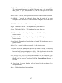
Front Chord: The chord length of the forward portion of the wedge. The value must
be greater than zero.
Middle Chord: The chord length of the middle portion of the wedge. The value must
be greater than or equal to zero.
Back Chord: The chord length of the back portion of the wedge. The value must be
greater than or equal to zero.
Front
Chord
Middle
Chord
Back
Chord
Span: The span of the wedge. The value must be greater than zero.
Front Droop: The droop of the front of the wedge. Measured parallel to the local z
axis.
Back Droop: The droop of the nose. Measured parallel to the local z axis.
Half Thickness: The half thickness of the middle portion of the wedge. The value
must be greater than zero.
Trailing Half Thickness: The half thickness of the base. The value must be greater
than or equal to zero.
Front Panels: The number of panels on the front portion of the wedge. The value
must be greater than zero.
Middle Panels: The number of panels on the middle portion of the wedge. The value
must be greater than zero.
45
Back Panels: The number of panels on the back portion of the wedge. The value
must be greater than zero.
Span Panels: The number of panels on the span of the wedge. The value must be
greater than zero.
Thickness Panels: The number of panels on the half thickness. The value must be
greater than zero.
Wedge Tips: Selection of a checkbox indicates whether a wedge tip should be
paneled. If the Starboard checkbox is selected then the starboard wedge tip will
be paneled. If the Port checkbox is selected then the port wedge tip will be
selected.
Inc. Base Load: If selected the base will not be used in the calculation of the
aerodynamic loads.
More...: Display the advanced settings dialog.
Box
The Box component has the following parameters.
X Shift: The amount that this component’s coordinate system is shifted backward
from the parent coordinate system. The value is measured along the parent
coordinate system x axis.
Y Shift: The amount that this component’s coordinate system is shifted starboard
from the parent coordinate system. The value is measured along the parent
coordinate system y axis.
Z Shift: The amount that this component’s coordinate system is shifted upward from
the parent coordinate system. The value is measured along the parent coordinate
system z axis.
Psi Rot: The amount, in degrees, that this component’s coordinate system is yawed.
The rotation transformations are applied in the same order as the aircraft Euler
angle system, i.e. yaw, pitch, and then roll, and are with respect to the parent
coordinate system.
Tht Rot: The amount, in degrees, that this component’s coordinate system is pitched.
The rotation transformations are applied in the same order as the aircraft Euler
angle system, i.e. yaw, pitch, and then roll, and are with respect to the parent
coordinate system.
46
Phi Rot: The amount, in degrees, that this component’s coordinate system is rolled.
The rotation transformations are applied in the same order as the aircraft Euler
angle system, i.e. yaw, pitch, and then roll, and are with respect to the parent
coordinate system.
Include Wake: If selected, wake panels will be included in the PANAIR calculation.
Local Wake: If selected, the wake will follow along the x axis of the parent
coordinate system otherwise the wake will follow along the x axis of the global
coordinate system.
Width: The width of the box. The width must be greater than zero.
Height: The height of the box. The height must be greater than zero.
Length: The length of the box. The length must be greater than zero.
Width Panels: The number of panels along the width. The width panels must be
greater than zero.
Height Panels: The number of panels along the height. The height panels must be
greater than zero.
Length Panels: The number of panels along the length. The length panels must be
greater than zero.
Include Face: A set of check boxes to specify if a face is active or not.
Two Sided: If selected, both sides of a box face are treated as external. If unselected
the outer side of each box face will be treated as external and the inner side will
be treated as if it was pointing inside the body. If this check box is selected then
at least one of the box faces should be disabled to open the box up.
Flow Through Front Face: If selected, the front face will be created as a flow
through face. A flow through face always has an inner and outer side so the Two
Sided check box must be unselected for Flow Through Front Face to be
selected.
Inc. Base Load: If selected the base will not be used in the calculation of the
aerodynamic loads.
More...: Display the advanced settings dialog.
47
Panel
The Panel component serves as a general surface component. Currently the user can
specify two types of surfaces. The first is a quadrilateral and the second is user defined.
For the quadrilateral, the x, y, and z coordinates for the four vertices are specified by the
user and panel corner points are determined by bilinear interpolation.
For the user defined option, the user specifies a python function in a script file and the
panel corner points are determined by executing that function once for each panel point.
The name of the function is expected to be ssToPt. Aero Troll uses jython for
interpreting the python file. An example of a Panel component python script file is
shown below
# beginning of file
#
# an example panel python script file
#
# ssx: chord ratio (0 <= ssx <= 1.0)
# ssy: span ratio (0 <= ssy <= 1.0)
# pp: a three element array to return point coordinates
#
pp[0]: x
#
pp[1]: y
#
pp[2]: z
def ssToPt(ssx,ssy,pp):
width = 2.0
length = 3.0
pp[0] = ssx*length
pp[1] = ssy*width
pp[2] = 1.0
#
# end of file
The script above will produce a rectangle 2 wide and 3 long. Three parameters are
passed to the ssToPt routine. The first two, ssx and ssy, are the ratios along the chord and
span for the panel corner points. The values will range between 0.0 and 1.0 inclusively.
The last parameter, pp, is a three element array which must be set inside the function to
the coordinates of the point specified by ssx and ssy. The first element of the array,
pp[0], is the x value. The second element of the array, pp[1], is the y value. And the
third element of the array, pp[2], is the z value.
A more complex exampling involving Panel components is given below in the NACA
RM L50H08 example section.
The Panel component has the following parameters.
X Shift: The amount that this component’s coordinate system is shifted backward
from the parent coordinate system. The value is measured along the parent
coordinate system x axis.
48
Y Shift: The amount that this component’s coordinate system is shifted starboard
from the parent coordinate system. The value is measured along the parent
coordinate system y axis.
Z Shift: The amount that this component’s coordinate system is shifted upward from
the parent coordinate system. The value is measured along the parent coordinate
system z axis.
Psi Rot: The amount, in degrees, that this component’s coordinate system is yawed.
The rotation transformations are applied in the same order as the aircraft Euler
angle system, i.e. yaw, pitch, and then roll, and are with respect to the parent
coordinate system.
Tht Rot: The amount, in degrees, that this component’s coordinate system is pitched.
The rotation transformations are applied in the same order as the aircraft Euler
angle system, i.e. yaw, pitch, and then roll, and are with respect to the parent
coordinate system.
Phi Rot: The amount, in degrees, that this component’s coordinate system is rolled.
The rotation transformations are applied in the same order as the aircraft Euler
angle system, i.e. yaw, pitch, and then roll, and are with respect to the parent
coordinate system.
Include Wake: If selected, wake panels will be included in the PANAIR calculation.
Local Wake: If selected, the wake will follow along the x axis of the parent
coordinate system otherwise the wake will follow along the x axis of the global
coordinate system.
Category: Currently the two types which can be chosen are Quadrilateral and User
Defined. Each category has different input requirements, which are listed below.
Quadrilateral: For the quadrilateral category the four corners of the quadrilateral
are required as input. The labels for the four corner points are: 1) Front,
Port, 2) Back, Port, 3) Front, Starboard, and 4) Back, Starboard. The x,
y, and z coordinate for each corner point is required.
User Defined: The user defined surface geometry requires the specification of
python file which contains the ssToPt function. How the path should be saved
to the Aero Troll session file depends on the setting of the Path radio buttons.
If the Path is set as Relative then the path will be saved relative to the path of
the executable. This requires that the script file be located at or below the
executable directory. If the Path is set as Absolute then the path will be
saved as an absolute path from the root directory. An absolute path is system
dependent whereas a relative one is not.
49
Type: The type of panel this component represents. The three choices are: 1)
Surface, 2) Base, or 3) Wake. A distinction between the Surface and Base types
exists only for a PANAIR analysis. For the local surface methods, the Surface
and Base types are treated the same. A Wake type only has meaning for a
PANAIR analysis. A Wake type does not influence the local surface method.
Two Sided: If selected this component is two sided, in other words both sides are
exterior surfaces.
Chord Panels: The number of panels along the chord.
Span Panels: The number of panels along the span.
Normal Vector Len.: The length of the normal vector.
Show NV: If selected, the normal vector will be shown.
More...: Display the advanced settings dialog.
Ground Plane
The ground plane component specifies that a x-y plane of symmetry should exist in the
analysis. The ground plane component is a flag to the analysis methods. The following
parameters are for visual purposes only and do not effect the interpretation of the flap. A
ground plane can only be added to an AT Analysis component. As mentioned in the
installation instructions in the beginning of this document, the PANAIR code must be
patched and recompiled for the Ground Plane component to work correctly.
X Shift: The amount that this component’s coordinate system is shifted backward
from the parent coordinate system. The value is measured along the parent
coordinate system x axis.
Y Shift: The amount that this component’s coordinate system is shifted starboard
from the parent coordinate system. The value is measured along the parent
coordinate system y axis.
Width: The width of the ground plane. This value is for display purposes only since
the ground plane extends to infinity in global coordinate systems x-y plane.
Length: The length of the ground plane. This value is for display purposes only since
the ground plane extends to infinity in global coordinate systems x-y plane.
Width Panels: The number of panels along the width of the ground plane. This value
is for display purposes only.
50
Length Panels: The number of panels along the length of the ground plane. This
value is for display purposes only.
Field Pts
The Field Pts component is used to query the flow field by means of a grid of points.
Currently, the Field Pts component only has meaning for a PANAIR analysis since
surface methods do not affect the flow field. The Field Pts component has the following
parameters.
X Shift: The amount that this component’s coordinate system is shifted backward
from the parent coordinate system. The value is measured along the parent
coordinate system x axis.
Y Shift: The amount that this component’s coordinate system is shifted starboard
from the parent coordinate system. The value is measured along the parent
coordinate system y axis.
Z Shift: The amount that this component’s coordinate system is shifted upward from
the parent coordinate system. The value is measured along the parent coordinate
system z axis.
Psi Rot: The amount, in degrees, that this component’s coordinate system is yawed.
The rotation transformations are applied in the same order as the aircraft Euler
angle system, i.e. yaw, pitch, and then roll, and are with respect to the parent
coordinate system.
Tht Rot: The amount, in degrees, that this component’s coordinate system is pitched.
The rotation transformations are applied in the same order as the aircraft Euler
angle system, i.e. yaw, pitch, and then roll, and are with respect to the parent
coordinate system.
Phi Rot: The amount, in degrees, that this component’s coordinate system is rolled.
The rotation transformations are applied in the same order as the aircraft Euler
angle system, i.e. yaw, pitch, and then roll, and are with respect to the parent
coordinate system.
Width: The width of the field points plane.
Length: The length of the field points plane.
Width Points: The number of points along the width of the field points plane.
Length Points: The number of points along the length of the field points plane.
51
Coordinate System
The Coordinate System component provides the means to introduce a coordinate system
within the model. Any component added to this component will inherit the coordinate
system of this component. The Coordinate System component has the following
parameters.
X Shift: The amount that this component’s coordinate system is shifted backward
from the parent coordinate system. The value is measured along the parent
coordinate system x axis.
Y Shift: The amount that this component’s coordinate system is shifted starboard
from the parent coordinate system. The value is measured along the parent
coordinate system y axis.
Z Shift: The amount that this component’s coordinate system is shifted upward from
the parent coordinate system. The value is measured along the parent coordinate
system z axis.
Psi Rot: The amount, in degrees, that this component’s coordinate system is yawed.
The rotation transformations are applied in the same order as the aircraft Euler
angle system, i.e. yaw, pitch, and then roll, and are with respect to the parent
coordinate system.
Tht Rot: The amount, in degrees, that this component’s coordinate system is pitched.
The rotation transformations are applied in the same order as the aircraft Euler
angle system, i.e. yaw, pitch, and then roll, and are with respect to the parent
coordinate system.
Phi Rot: The amount, in degrees, that this component’s coordinate system is rolled.
The rotation transformations are applied in the same order as the aircraft Euler
angle system, i.e. yaw, pitch, and then roll, and are with respect to the parent
coordinate system.
52
Group
The Group component has the same feature set as the Coordinate System component. In
addition, the Group component provides a container for which all the integrated loads and
moments of the attached components will be combined. The combined loads will be
non-dimensionalized by the Group component reference areas and lengths.
The Group component has the following parameters.
X Shift: The amount that this component’s coordinate system is shifted backward
from the parent coordinate system. The value is measured along the parent
coordinate system x axis.
Y Shift: The amount that this component’s coordinate system is shifted starboard
from the parent coordinate system. The value is measured along the parent
coordinate system y axis.
Z Shift: The amount that this component’s coordinate system is shifted upward from
the parent coordinate system. The value is measured along the parent coordinate
system z axis.
Psi Rot: The amount, in degrees, that this component’s coordinate system is yawed.
The rotation transformations are applied in the same order as the aircraft Euler
angle system, i.e. yaw, pitch, and then roll, and are with respect to the parent
coordinate system.
Tht Rot: The amount, in degrees, that this component’s coordinate system is pitched.
The rotation transformations are applied in the same order as the aircraft Euler
angle system, i.e. yaw, pitch, and then roll, and are with respect to the parent
coordinate system.
Phi Rot: The amount, in degrees, that this component’s coordinate system is rolled.
The rotation transformations are applied in the same order as the aircraft Euler
angle system, i.e. yaw, pitch, and then roll, and are with respect to the parent
coordinate system.
sRef: The reference area used to non-dimensionalize the aerodynamic forces and
moments. The value must be greater than zero.
lRef: The reference length used to non-dimensionalize the longitudinal aerodynamic
moments. The value must be greater than zero.
bRef: The reference length used to non-dimensionalize the lateral aerodynamic
moments. The value must be greater than or equal to zero. If the value is equal to
zero then lRef will be substituted for bRef.
53
xMom: The x value for the moment center measured in the local coordinate system.
Positive is rearward.
yMom: The y value for the moment center measured in the local coordinate system.
Positive is starboard.
zMom: The z value for the moment center measured in the local coordinate system.
Positive is up.
CREATING LINKS
A user can reference a geometry component from one location to another in the
component tree by creating a link. To create a link, move the mouse cursor over a
geometry component and select the geometry component by clicking and holding down
the left mouse button. The cursor appearance will change to that seen in the figure below
or a slash. Then drag the component to the desired location in the component tree. If the
location is an invalid location then the cursor will be a slash, otherwise it will be as seen
in the figure below. In the example shown below (my version of a pod racer), an AT
Analysis component has been created with four Coordinate System components. A
Group component has been added to the first Coordinate System component and a
Nose+Body and Fin Set component have been added to the Group component. For this
case, the body length for the Nose+Body is zero, the number of base panels for the
Nose+Body is zero, the wake for the Nose+Body is deactivated, the root chord for the Fin
Set is set to 1.0, the tip chord for the Fin Set is set to 0.5, the span for the Fin Set is set to
0.5, the Fin Set is shifted back by 2.0, fins 2 through 4 are deleted, and the Theta Panels
for the remaining fin is set to 12. Next the link is created by left clicking on the Group
component and holding down the mouse button. Then, the Group component is dragged
to the second Coordinate System component, as shown below, and released.
54
55
The above steps are repeated for the last two remaining Coordinate System components.
The Aero Troll window now appears as in the following figure.
56
Since the coordinate systems have the same position parameters, the four groups overlay
one another. To separate the the groups, the Z Shift, Y Shift, and Phi Rot parameters for
the Coordinate System components are set so the fin tips touch and a body is at 12
o’clock, 3 o’clock, 6 o’clock, and 9 o’clock. The configuration forms a “+”. After
changing the view, the image appears as follows.
57
Next, the AT Analysis Mach parameter is set to 1.5 and the case is executed. The
resulting image is shown below.
58
If the a geometry parameter of the original Nose+Body or Fin Set is modified, then all the
geometries are modified. For example, in the figure below the first Fin Set tip chord has
been changed to 1.0.
ANALYSIS METHODS
Currently Aero Troll has the capability to execute two classes of analysis methods: 1)
PANAIR, and 2) Local Surface Methods. In both cases, the description given will be
very brief. The reader is STRONGLY encouraged to read the references relating to these
two methodologies.
PANAIR
PANAIR is an external program and must be obtained from www.pdas.com. The reader
is encouraged to read the documentation which comes with PANAIR.
Local Surface Methods
Included with Aero Troll are a set of supersonic/hypersonic windward and leeward local
surface methods. The selection set of windward methods are: 1) modified Newtonian, 2)
tangent-wedge, and 3) tangent-cone. The selection set of leeward methods are: 1) p∞ and
2) Prandtl-Meyer expansion. The impact methods are based on those described in the
59
Program Formulation volume of the Mark 1V Supersonic-Hypersonic Arbitrary-Body
Computer Program documents (http://handle.dtic.mil/100.2/AD778444). The user is
encouraged to review the sections pertaining to the above method local surface methods
within the program formulation volume. The current local surface methods in Aero Troll
do not take into account shielding.
DISCUSION
PANAIR
Below are several topics regarding PANAIR and Aero Troll.
Paneling for PANIR
The setup of a proper input deck for PANAIR can be complex. Some of the issues to
insure are: 1) Control points are not overly influenced by panels other than the panel the
control point belongs to, 2) Network edges are abutted correctly to maintain continuity of
doublet and source strengths, 3) Wakes are set up correctly to adequately model the
physical wake and to ensure gaps between wake sheets do not exist.
Listed below are a couple of helpful remarks regarding usage. The example geometry
used in the remarks comes from the NASA TM-2001-210652, Body+Fin 11 example
which is described later.
1) Panels should match up.
An example of this is the need to match up the number of circumferential panels
between a forward and aft component. Shown below is a geometry with, going from
forward to back, a Nose+Body, Fin Set, and Body component.
60
In this case each component has twelve panels on the circumference.
61
If the number of panels on the circumference for the Nose+Body component is
changed to eleven then the panels would not align. This is shown below.
Misaligned
Panels
Under some circumstances this will cause the PANAIR panel networks to butt up
incorrectly.
62
2) A Body component should be segmented so the segment edges match up with wakes.
If an edge of a wake is connected to a body then that wake must connect to a panel
network edge. Each Body segment, as described in the Body component section, is
described by a unique panel network. Therefore, if a wake passes next to a Body
component, that Body component must be segmented so the wake connects to a
segment edge. This is shown in the image below.
In this case a fin, and thus wake, is at 90 and 270 degrees. Therefore the body has
two body segments. One body edge has an edge at 90 degrees and the other has one
at 270 degrees. The fact that the wake connection to the body edge is valid is
indicated by the blue wake panel grid shown in the image above.
63
For the following image the first body segment was give an edge at 100 degrees
instead of 90 degrees.
Since the wake from the starboard fin (90 degrees) no longer connects to a body
segment edge (100 degrees) a panel network for the wake was not created. This can
be seen in the image above for the starboard wake.
64
3) Physical deflections should be used with caution.
Physical deflections cause two problems for PANAIR. First, a fin panel may have
excessive influence on a body panel control point since the fin panel edge may be too
close to a body panel control point. Second, the wake will not attach itself to a body
edge segment. This is shown in the figure below for a 20 degree deflection of the
starboard fin.
In the figure above it can be seen that the root edge of the fin panel network passes
close to the body panel control points. It can also be seen that the fin wake is not
attached to the body and therefore odd panel strengths may result.
When using PANAIR, the deflections for the fins should be handled by the boundary
conditions. This is specified by selecting the Def. In B.C. checkbox.
65
4) Wakes should not intersect panels.
If panels intersect or overlay one another, then the results will be indeterminate or
incorrect. Two examples of wakes intersecting panels are given. The first example is
of a wake from a forward fin intersecting a rear fin. This is shown in the figure
below.
In this example the rear fins were shifted down by two degrees and then given an
upward dihedral of 10 degrees. If the rear fins were actually in the plane of the wake
a warning would have been given that “Multiple trailing legs can not be accounted
for.” Future versions of Aero Troll will be more robust in regards to handling a wake
from a forward fin set to a rear one.
66
Another example of a wake intersection is shown below.
5) Only one fin set should be modeled with PANAIR.
Because of the current limitations with wakes, as described in item 4 above, only one
fin set should be modeled.
Input files
When Aero Troll sets up the execution of a PANAIR run it creates an input file with a
random name, places the input file, for Windows XP, in the
AeroTroll_v020b\AT_Data\PC\at_panair directory, and creates a working directory for
PANAIR with the same base name as the input file. For Linux the file and working
directory is placed in the AeroTroll_v020b/AT_Data/LINUX/at_panair directory. Once
Aero Troll is finished with the working directory it is deleted.
Under some conditions, such as if Aero Troll crashes (which happens very infrequently,
but it does happen), the input file and directory will not be deleted. Therefore,
occasionally, it is necessary to go into the at_panair directory and delete any input files
and directories which exist.
67
One more item to mention about PANAIR input files. The input file for PANAIR is
formatted therefore the input fields are of fixed width. Aero Troll maximizes the number
of significant figures it can place in a field by selecting either scientific notation or
decimal floating point. The consequence is that scaling the geometry may change the
number of significant figures in the input file and thus affect the results a little.
Determination of pressure
Pressures are determined by Aero Troll using the compressible Bernoulli equation with
velocities calculated by PANAIR.
Determination of loads
The loads are determined by integrating p-p∞ over the body.
EXAMPLES
NASA TM-2001-210652, Body+Fin 11
The following example describes the construction of a simple Fin-Body configuration
given in NASA TM-2001-210653. A PDF version of the TM can be downloaded from
the NASA technical report server, ntrs.nasa.gov.
For this example the diameter of the body is 3.0, the nose length is 9.0, and the overall
length is 36.0. The body has an ogive nose. There are two fins, one on the starboard and
one on the port side. The fin span is 3.0, the root chord is 6.0, the tip chord is 3.0, and the
leading edge sweep is 45.0 degrees. The hinge line is located at 60% of the root chord
and connects with the body at 27.0 rearward from the nose tip. The reference area is
equal to the base area, the reference length is equal to the diameter, and the moment
center is located at an x location of 21.0.
Four components will be created: 1) an AT Analysis Component, 2) a Nose+Body
component, 3) a Fin Set component, 4) and a Body component.
The xml input file for this case is in the examples directory.
AT Analysis Component
First, start Aero Troll by double clicking on AeroTroll_win script under Windows XP or
executing AeroTroll_lin under Linux. Once Aero Troll is started, create the AT Analysis
component by right clicking on the working area of Components panel to show the
component tree popup menu and then select AT Analysis from the Add menu. Once the
AT Analysis component is created, right click on the AT Analysis component node and
select the Edit menu item from the component popup menu to show the AT Analysis edit
panel. In the At Analysis edit panel set the following parameters to the values given
below.
68
sRef:
lRef:
xMom:
7.0686
3.0
21.0
Finally click on the Accept button and close the Edit Window. The Aero Troll window
should look like the following figure.
69
Next, create a Nose+Body component by right clicking on the AT Analysis component
node and selecting Nose+Body from the Add submenu of the AT Analysis component
popup menu. Once the Nose+Body is created, right click on the Nose+Body component
node to display the Nose+Body component popup menu and select the Edit menu item.
In the Nose+Body edit panel set the following parameters to the values given below.
Include Wake:
Nose Type:
Nose Radius:
Nose Length:
Body Length:
Body Panels:
Base Panels:
Unselected
Ogive
1.5
9.0
14.4
16
0
After completion, the Edit panel for the Nose+Body component should look like the
following figure.
70
It is important that the wake is not included and that the base is removed by setting the
Base Panels to zero since the Body component, to be created later, will supply the wake
and base for the body.
71
Next, select the Accept button and the Aero Troll window should like the following
figure.
Next, create a Fin Set component by right clicking on the AT Analysis component node
and selecting Fin Set from the Add submenu of the AT Analysis component popup
menu. Once the Fin Set is created, right click on the Fin Set component node to display
the component popup menu and select the Edit menu item. In the Fin Set edit panel set
the following parameters to the values given below.
X Shift:
Body Wake:
Body Radius:
Root Chord:
Tip Chord:
Span:
LE Sweep:
Hinge Line:
Base Panels:
Def. In B.C.:
23.4
Unselected
1.5
6.0
3.0
3.0
45.0
0.6
0
Selected
72
Next, delete fins 3 and 4 by selecting the Delete Fin button for those fins. Then set
Theta for the first fin to 90.0 degrees, Theta for the second fin to 270.0 degrees, and
Theta Panels to 6 for both fins.
After completion, the Edit panel for the Fin Set component should look like the following
two figures.
73
Just as with the Nose+Body component, it is important that the body wake is not included
and that the base is removed by setting the Base Panels to zero since the Body
component, to be created next, will supply the wake and base for the body.
74
Next, select the Accept button, and the top and side views should look like the following
two figures.
75
Next, create a Body component by right clicking on the AT Analysis component node
and selecting Body from the Add submenu of the AT Analysis component popup menu.
Once the Body is created, right click on the Body component node to display the
component popup menu and select the Edit menu item. In the Body edit panel set the
following parameters to the values given below.
X Shift:
Forward Radius:
Aft Radius:
Body Length:
Inc. Base Load:
29.4
1.5
1.5
6.6
Unselected
Next, add another body segment by clicking on the Add Segment button at the bottom of
the Body edit panel. Then set Theta for the first body segment to 90.0 degrees, Theta
for the second body segment to 270.0 degrees, and Theta Panels to 6 for both body
segments.
76
After completion, the Edit panel for the Body component should look like the following
figure.
77
Next, select the Accept button, and the top and side views should look like the following
two figures.
78
For the wind tunnel model in TM-2001-210652 the “body internal diameter was beveled
to the outer diameter at the base of the model to allow the internal pressures to act over
the entire base area.” Also, the “CA due to cavity pressures was subtracted from the
measured balance CA.” Therefore, to mimic this in the Aero Troll model, the Inc. Base
Load for the Body component is unselected.
This completes the geometry buildup for this example.
Wing T-Tail
The following example is of a generic wing-body-tee tail configuration. This geometry is
made up of one Nose+Body component, three Fin Set components, and one Body
component.
After creating an AT Analysis component, create a Nose+Body component with the
following parameters.
Include Wake:
Nose Type:
Nose Length:
Body Length:
Base Panels:
Unselected
Ogive
3.5
1.5
0
79
The Base Panels is set to zero and Include Wake is unselected since the body base and
wake are handled by another component.
The next component to be created is a Fin Set component with the following parameters.
X Shift:
Body Wake:
Root Chord:
Tip Chord:
Span:
Base Panels:
5
Unselected
3.0
0.5
2.5
0
Next delete the fins at 0 degrees and 180 degrees and set the Theta Panels for the two
remaining fins to 6. The Base Panels is set to zero and Include Wake is unselected
since the body base and wake are handled by another component.
The geometry up to this point is shown in the figure below.
The next component to be created, which models the body segment between the wing and
tail, is a Body component with the following parameters.
80
X Shift:
Include Wake:
Body Length:
Base Panels:
8.0
Unselected
2.5
0
For this component a second segment should be added. The Theta parameter for the first
segment should be set to 90 degrees and the Theta parameter for the second segment
should be set to 270 degrees. The Theta Panels parameter for both segments should be
set to 6. Setting the segment edges at 90 and 180 degrees allows the wake from the
wings to attach to the body. The Base Panels is set to zero and Include Wake is
unselected since the body base and wake are handled by another component. The current
geometry is shown below.
The next component to be created, which models the vertical tail, is a Fin Set component
with the following parameters.
X Shift:
Root Chord:
Tip Chord:
Span:
LE Sweep:
10.5
2.0
1.0
1.5
50.0
81
For this component the Include Fin checkbox for fin 2, 3, and 4 should be unselected.
The segment edges located at 90 and 180 degrees allows the wing wakes to attach to the
body. The current geometry is shown below.
The next component, which models the horizontal tee tail, is a Fin Set component with
the following parameters.
X Shift:
Z Shift:
Body Radius:
Root Chord:
Top Chord:
Span:
LE Sweep:
Fins Only:
12.2876303889
2.0
0.0
1.0
0.5
1.5
30.0
Selected
82
Next delete the fins at 0 and 180 degrees. For this case the X Shift requires as many
significant figures as possible to insure that the horizontal fin matches up to the tip of the
vertical fin. The geometry is shown below.
This completes the geometry buildup for this example.
NACA RM L50H08
The following example describes the construction of the wing body configuration given
in NASA RM L50H08. A PDF version of the RM can be downloaded from the NASA
technical report server, ntrs.nasa.gov.
This example relies on the use of python scripts to define the body and wing. The python
scripts are somewhat involved so they will not be described in this section. However, the
scripts are included in the appendix and the user is encouraged to look them over or to
dig into the actual scripts located in the examples/NACA_RM_L50H08/Scripts directory.
Currently, Aero Troll does not have a graphical means of allowing the user to
interactively construct arbitrary geometry segments. However, python scripts can be
used to perform this task. Hopefully a user interface for constructing arbitrary geometry
segments will be available in future versions of Aero Troll.
83
This geometry is made up of eight Panel components and one Body component. Six of
the Panel components will be used for the body and two for the wing.
After creating an AT Analysis component, create a Panel component and name it
“ForBody Top”. Next, set the component’s parameters as follows.
Categroy:
Function File:
Two Sided:
Chord Panels:
Span Panels:
User Defined
examples\NACA_RM_L50H08\Scripts\NACA_RM_L50H08_for_body.py
unselected
10
6
To create the forebody bottom panel, copy the ForBody Top component and paste it
under the AT Analysis component. To do this, right click on the ForBody Top
component and select the Copy menu item. Next, right click on the AT Analysis
component and select the Paste menu item. A new ForBody Top component will be
placed under the AT Analysis component. Next, rename the new ForBody Top
component to “ForBody Bot” by right clicking on the new ForBody Top component and
selecting the Rename menu item. The Aero Troll window will look like the following
figure.
84
To finish the ForBody Bot component, set its parameters as follows.
Phi Rot:
180.0
The next set of panel components will be used to define the midsection. The
methodology is similar to that of building the forebody. Create a Panel component and
name it “MidBody Top”. Next, set the component’s parameters as follows.
Categroy:
Function File:
Two Sided:
Chord Panels:
Span Panels:
User Defined
examples\NACA_RM_L50H08\Scripts\NACA_RM_L50H08_mid_body.py
unselected
5
6
To create the midbody bottom panel, copy the MidBody Top component and paste it
under the AT Analysis component. To do this, right click on the MidBody Top
component and select the Copy menu item. Next, right click on the AT Analysis
component and select the Paste menu item. A new MidBody Top component will be
placed under the AT Analysis component. Next, rename the new MidBody Top
component to “MidBody Bot” by right clicking on the new MidBody Top component and
selecting the Rename menu item.
Next set the MidBody Bot component parameters as follows.
Phi Rot:
180.0
The next set of panel components will be used to define the aftbody. The methodology is
similar to that of building the forebody and midbody. Create a Panel component and
name it “AftBody Top”. Next, set the component’s parameters as follows.
Categroy:
Function File:
Two Sided:
Chord Panels:
Span Panels:
User Defined
examples\NACA_RM_L50H08\Scripts\NACA_RM_L50H08_aft_body.py
unselected
10
6
To create the aftbody bottom panel, copy the AftBody Top component and paste it under
the AT Analysis component. Next, rename the new AftBody Top component to
“AftBody Bot”.
Next set the AftBody Bot component parameters as follows.
Phi Rot:
180.0
85
The current wing component for Aero Troll requires that the root and tip chord be
straight. Since the wings in this example have curved root chords, panel components will
be used to describe the wings in this example.
Create a Panel component and name it “Star Wing”.
parameters as follows.
Include Wake:
Categroy:
Function File:
Chord Panels:
Span Panels:
Next, set the component’s
Two Sided
User Defined
examples\NACA_RM_L50H08\Scripts\NACA_RM_L50H08_wing.py
5
10
To create the port side wing panel, copy the Star Wing component and paste it under the
AT Analysis component. Next, rename the new Star Wing component to “Port Wing”.
Next set the Port Wing component parameters as follows.
Phi Rot:
180.0
The next component, which models the sting, is a Body component with the following
parameters.
X Shift:
Forward Radius:
Aft Radius:
Body Length:
33.3333
0.8333
0.8333
10.0
For this component a second segment should be added. The Theta parameter for the first
segment should be set to 90 degrees and the Theta parameter for the second segment
should be set to 270 degrees. The Theta Panels parameter for both segments should be
set to 6. Setting the segment edges at 90 and 180 degrees allows the wake from the
wings to attach to the body. The current geometry is shown below.
86
This completes the geometry buildup for this example.
87
APPENDIX A
Script Listings for NACA RM L50H08 Example
######## beginning of NACA_RM_L50H08.py script ########
import math
# Tridiagonal solver
# NOTE: order is as follows...
#
# [b1 c1
#
a2 b2 c2
#
a3 b3 c3
#
a4 b4]
#
def TriDiag(aa,bb,cc,dd):
# get size
mm = len(dd)
# set first value
dd[0] = dd[0]/bb[0]
# loop through other values
for ii in range(1,mm):
cc[ii-1] = cc[ii-1]/bb[ii-1]
bb[ii]
= bb[ii]-aa[ii]*cc[ii-1]
dd[ii]
= (dd[ii]-aa[ii]*dd[ii-1])/bb[ii]
# back substitute
for ii in range(mm-1,0,-1):
dd[ii-1] = dd[ii-1]-cc[ii-1]*dd[ii]
#
# end of TriDiag method
#
# Cubic Spline method
# Based on spline method from:
# Numerical Methods for Engineers, Second Edition
# Steven C. Chapra, Raymond P. Canale
def CubicSpline(xx,yy,dd,fDY1DX,fDYNDX):
# get number of points
mm = len(xx)
# create the arrays for the tridiagonal system
aa = [0]*mm
bb = [0]*mm
cc = [0]*mm
# set values
for ii in range(1,mm-1):
aa[ii] =
xx[ii] - xx[ii-1]
bb[ii] = 2.0*(xx[ii+1]-xx[ii-1])
cc[ii] =
xx[ii+1]-xx[ii]
dd[ii] = 6.0*((yy[ii+1]-yy[ii])/(xx[ii+1]-xx[ii]) - \
(yy[ii]-yy[ii-1])/(xx[ii]-xx[ii-1]))
# set first values
if (fDY1DX != 0): # set starting first derivative to zero
aa[0]
= 0.0
bb[0]
= 2.0
cc[0]
= 1.0
dd[0]
= 6.0*(yy[1]-yy[0])/((xx[1]-xx[0])*(xx[1]-xx[0]))
else:
# set starting second derivative to zero
aa[0]
= 0.0
bb[0]
= 1.0
cc[0]
= 0.0
dd[0]
= 0.0
# set last
if (fDYNDX
aa[mm-1]
bb[mm-1]
cc[mm-1]
dd[mm-1]
else:
aa[mm-1]
bb[mm-1]
cc[mm-1]
values
!= 0): # set ending first derivative to zero
= 0.0
= 2.0
= 1.0
=-6.0*(yy[mm-1]-yy[mm-2])/((xx[mm-1]-xx[mm-2])*(xx[mm-1]-xx[mm-2]))
# set ending second derivative to zero
= 0.0
= 1.0
= 0.0
88
dd[mm-1] = 0.0
# solve
TriDiag(aa,bb,cc,dd)
#
# end of cubic spline method
#
# Cublic Spline Evaluation method
# Based on spline method from:
# Numerical Methods for Engineers, Second Edition
# Steven C. Chapra, Raymond P. Canale
def CubicSplineYY(xin,xx,yy,dd):
# get number of points
mm = len(xx)
# find the bracketing values
for ii in range(1,mm):
if ((xin >= xx[ii-1] and xin <= xx[ii]) or
(xin <= xx[ii-1] and xin >= xx[ii])):
break
if (ii == mm):
raise Exception("CubicSplineYY: Bracketing values could not be found.")
# return value
dx = xx[ii] - xx[ii-1]
dx1 = xx[ii] - xin
dx2 = xin
- xx[ii-1]
return (dd[ii-1]*dx1*dx1*dx1 + dd[ii]*dx2*dx2*dx2)/(6.0*dx) + \
(yy[ii-1]/dx - dd[ii-1]*dx/6.0)*dx1 + \
(yy[ii]/dx
- dd[ii]*dx/6.0)*dx2
#
# end of cubic spline evaluation method
#
# Cublic Spline Derivative method
# Based on spline method from:
# Numerical Methods for Engineers, Second Edition
# Steven C. Chapra, Raymond P. Canale
def CubicSplineDY(xin,xx,yy,dd):
# get number of points
mm = len(xx)
# find the bracketing values
for ii in range(1,mm):
if ((xin >= xx[ii-1] and xin <= xx[ii]) or
(xin <= xx[ii-1] and xin >= xx[ii])):
break
if (ii == mm):
raise Exception("CubicSplineYY: Bracketing values could not be found.")
# return value
dx = xx[ii] - xx[ii-1]
dx1 = xx[ii] - xin
dx2 = xin
- xx[ii-1]
return 3.0*(-dd[ii-1]*dx1*dx1 + dd[ii]*dx2*dx2)/(6.0*dx) - \
(yy[ii-1]/dx - dd[ii-1]*dx/6.0) + \
(yy[ii]/dx
- dd[ii]*dx/6.0)
#
# end of cubic spline derivative method
#
#
# beginning of bodySSToPts method
#
def bodySSToPt(ssx,ssy,pp):
if (ssx == 1.0):
pp[0] = 33.3333
radius = 1.6666/2.0
else:
pp[0] = ssx*100/3
radius = 40*CubicSplineYY(ssx*5/6,xl,rl,dl)
if ssy == 1.0:
angle = 0.0
else:
angle = ssy*2.0*math.pi
pp[1] = radius*math.sin(angle)
pp[2] = -radius*math.cos(angle)
#
# end of bodySSToPts method
#
89
#
# beginning of forBodySSToPt method
#
def forBodySSToPt(ssx,ssy,pp):
if (ssx == 0.0):
pp[0] = 0.0
radius = 0.0
elif (ssx == 1.0):
pp[0] = xx1A
radius = yy1A
else:
pp[0] = ssx*xx1A
radius = 40*CubicSplineYY(pp[0]/40,xl,rl,dl)
if ssy == 0.0:
pp[1] = radius
pp[2] = 0.0
elif ssy == 1.0:
pp[1] = -radius
pp[2] = 0.0
else:
angle = ssy*math.pi
pp[1] = radius*math.cos(angle)
pp[2] = radius*math.sin(angle)
#
# end of forBodySSToPt method
#
#
# beginning of midBodySSToPt method
#
def midBodySSToPt(ssx,ssy,pp):
if (ssx == 0.0):
pp[0] = xx1A
radius = yy1A
elif (ssx == 1.0):
pp[0] = xx1B
radius = yy1B
else:
pp[0] = xx1A + ssx*(xx1B - xx1A)
radius = 40*CubicSplineYY(pp[0]/40,xl,rl,dl)
if ssy == 0.0:
pp[1] = radius
pp[2] = 0.0
elif ssy == 1.0:
pp[1] = -radius
pp[2] = 0.0
else:
angle = ssy*math.pi
pp[1] = radius*math.cos(angle)
pp[2] = radius*math.sin(angle)
#
# end of midBodySSToPt method
#
#
# beginning of aftBodySSToPt method
#
def aftBodySSToPt(ssx,ssy,pp):
if (ssx == 0.0):
pp[0] = xx1B
radius = yy1B
elif (ssx == 1.0):
pp[0] = 33.3333
radius = 1.6666/2.0
else:
pp[0] = xx1B + ssx*(33.333 - xx1B)
radius = 40*CubicSplineYY(pp[0]/40,xl,rl,dl)
if ssy == 0.0:
pp[1] = radius
pp[2] = 0.0
elif ssy == 1.0:
pp[1] = -radius
pp[2] = 0.0
else:
angle = ssy*math.pi
pp[1] = radius*math.cos(angle)
pp[2] = radius*math.sin(angle)
#
# end of aftBodySSToPt method
#
90
#
# beginning of wingSSToPt method
#
def wingSSToPt(ssx,ssy,pp):
# get root value
if (ssx == 0.0):
wx1 = xx1A
wy1 = yy1A
elif (ssx == 1.0):
wx1 = xx1B
wy1 = yy1B
else:
wx1 = xx1A + ssx*(xx1B - xx1A)
wy1 = 40*CubicSplineYY(wx1/40,xl,rl,dl)
# get tip value
if (ssx == 0.0):
wx2 = xx2A
wy2 = yy2A
elif (ssx == 1.0):
wx2 = xx2B
wy2 = yy2B
else:
wx2 = xx2A + ssx*(xx2B - xx2A)
wy2 = yy2A + ssx*(yy2B - yy2A)
# set values
if (ssy == 0.0):
pp[0] = wx1
pp[1] = wy1
elif (ssy == 1.0):
pp[0] = wx2
pp[1] = wy2
else:
pp[0] = wx1 + ssy*(wx2 - wx1)
pp[1] = wy1 + ssy*(wy2 - wy1)
pp[2] = 0.0
#
# end of wingSSToPt method
#
# set up global values
# define body shape
xl = [0.0000,
0.0050,
0.0075,
0.0125,
0.0250,
0.0500,
0.0750,
0.1000,
0.1500,
0.2000,
0.2500,
0.3000,
0.3500,
0.4000,
0.4500,
0.5000,
0.5500,
0.6000,
0.6500,
0.7000,
0.7500,
0.8000,
0.8333,
0.8500,
0.9000,
0.9500,
1.0000]
rl = [0.00000,
0.00231,
0.00298,
0.00428,
0.00722,
0.01205,
0.01613,
0.01971,
0.02593,
0.03090,
0.03465,
91
0.03741,
0.03933,
0.04063,
0.04143,
0.04167,
0.04130,
0.04024,
0.03842,
0.03562,
0.03128,
0.02526,
0.02083,
0.01852,
0.01125,
0.00439,
0.00000]
dl = [0]*len(xl)
# create slpine for body shape
CubicSpline(xl,rl,dl,0,0)
# calculate wing corner locations
cc1 = 20 - 5.5 # quarter chord location at centerline
cc2 = 20 + 6.5 # quarter chord location at wing tip
xx1A = cc1 - 0.25*7.5
yy1A = 0.0
xx1B = cc1 + 0.75*7.5
yy1B = 0.0
xx2A = cc2 - 0.25*4.5
yy2A = 12.0
xx2B = cc2 + 0.75*4.5
yy2B = 12.0
# calculate intercept of wing leading edge with body
xi
= xx1A # initial guess
dywdx = (yy2A - yy1A)/(xx2A - xx1A) # slope for wing
while 1:
yw
= yy1A + dywdx*(xi - xx1A)
yb
= 40*CubicSplineYY(xi/40.0,xl,rl,dl)
dy
= yw - yb
dybdx = CubicSplineDY(xi/40.0,xl,rl,dl)
dx
= dy/(dybdx - dywdx)
xi
= xi + dx
if (math.fabs(dx) < 1.0e-14):
break
# set values
yy1A = yy1A + dywdx*(xi - xx1A)
xx1A = xi
# calculate intercept of wing tail edge with body
xi
= xx1B # initial guess
dywdx = (yy2B - yy1B)/(xx2B - xx1B) # slope for wing
while 1:
yw
= yy1B + dywdx*(xi - xx1B)
yb
= 40*CubicSplineYY(xi/40.0,xl,rl,dl)
dy
= yw - yb
dybdx = CubicSplineDY(xi/40.0,xl,rl,dl)
dx
= dy/(dybdx - dywdx)
xi
= xi + dx
if (math.fabs(dx) < 1.0e-14):
break
# set values
yy1B = yy1B + dywdx*(xi - xx1B)
xx1B = xi
######## ending of NACA_RM_L50H08.py script ########
######## beginning of NACA_RM_L50H08_for_body.py script ########
import math
from examples.NACA_RM_L50H08.Scripts import NACA_RM_L50H08
reload(NACA_RM_L50H08)
def ssToPt(ssx,ssy,pp):
NACA_RM_L50H08.forBodySSToPt(ssx,ssy,pp)
######## ending of NACA_RM_L50H08_for_body.py script ########
######## beginning of NACA_RM_L50H08_mid_body.py script ########
import math
from examples.NACA_RM_L50H08.Scripts import NACA_RM_L50H08
92
reload(NACA_RM_L50H08)
def ssToPt(ssx,ssy,pp):
NACA_RM_L50H08.midBodySSToPt(ssx,ssy,pp)
######## ending of NACA_RM_L50H08_mid_body.py script ########
######## beginning of NACA_RM_L50H08_aft_body.py script ########
import math
from examples.NACA_RM_L50H08.Scripts import NACA_RM_L50H08
reload(NACA_RM_L50H08)
def ssToPt(ssx,ssy,pp):
NACA_RM_L50H08.aftBodySSToPt(ssx,ssy,pp)
######## ending of NACA_RM_L50H08_aft_body.py script ########
######## beginning of NACA_RM_L50H08_wing.py script ########
import math
from examples.NACA_RM_L50H08.Scripts import NACA_RM_L50H08
reload(NACA_RM_L50H08)
def ssToPt(ssx,ssy,pp):
NACA_RM_L50H08.wingSSToPt(ssx,ssy,pp)
######## ending of NACA_RM_L50H08_wing.py script ########
93