Download Phase 3 data release description

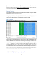
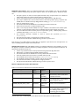
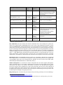
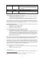
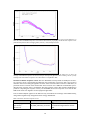
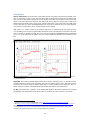
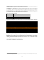
ESO Phase 3 Data Release Description for Internal Data Products
Data Collection
Release Number
Program Type
Data Provider
Document Date
Document version
Document Author
On-line version
XSHOOTER_ECHELLE
1
Internal
ESO, Quality Control Group
<09.05.2014>
1.0
Reinhard Hanuschik
http://www.eso.org/qc/PHOENIX/XSHOOTER/processing.html
Abstract
This is the release of reduced 1D spectra from the XSHOOTER1 spectrograph, ECHELLE (SLIT)
mode (as opposed to the IFU mode). All spectra have been reduced under the assumption of pointlike sources. This release is an open stream release, it includes so far archived XSHOOTER data and
will be continued into the future. The processing scheme is as homogeneous as possible.
The selected data cover the vast majority of the entire XSHOOTER data archive, from the begin of
operations in October 2009 until present. The data have been reduced with the XSHOOTER pipeline, version xshoo-2.3 and higher. All data have their instrument signature removed: they have
been de-biased, flat-fielded, wavelength-calibrated, order-merged, extracted, sky-subtracted and
finally flux-calibrated. Telluric absorption has not been corrected for. The pipeline output products
come in the ESO 1D standard binary table2, along with some ancillary files.
The processing is performed by the Quality Control Group in an automated process. The pipeline
processing uses the archived, closest-in-time, quality-controlled, and certified master calibrations.
It is important to note that the reduction process itself is automatic, while the quality assessment
and certification of the master calibrations was (and still is) human-supervised. The overall data
content will grow with time as new data are being acquired and processed (approximately with
monthly cadence and with a delay of 1 or 2 months).
These products are called Internal Data Products (IDPs) since they are produced in-house, as opposed to externally provided data products. The IDPs cover many different science cases (defined
by their parent programmes, in the case of XSHOOTER many hundreds).
The data format follows the ESO 1D spectroscopic standard2 for phase-3 data products. Each spectrum is a multi-column binary table. There is one product file for each set of input raw files. The set
of input raw files is template-based for the NODDING and OFFSET data, and file-based for STARE
data. The XSHOOTER IDPs always come per arm: UVB, VIS, or NIR.
This data release offers science-grade data products, with the instrumental signature and sky background removed, flux-calibrated, with error estimates and quality flags, and with a list of known
shortcomings. They are considered to be ready for scientific analysis. They are expected to be useful for any kind of medium-to-high resolution spectroscopic research, including abundance and
line profile studies, and radial velocity studies. For studies of energy distributions the researcher
should keep in mind that the XSHOOTER instrument is a medium-to-high resolution spectrograph,
designed for stability and throughput. It is usually not operated to achieve high-precision spectrophotometry, unless the wide slit is used. Slit losses have to be expected, and they may differ from
arm to arm. There has been no attempt to correct for telluric absorption lines; this might affect
certain science applications.
Disclaimer. Data have been pipeline-processed with the best available calibration data. However,
1
2
http://www.eso.org/sci/facilities/paranal/instruments/xshooter.html
http://www.eso.org/sci/observing/phase3/p3sdpstd.pdf
1
please note that the adopted reduction strategy may not be optimal for the original scientific purpose of the observations, nor for the scientific goal of the archive user.
You may also want to consult the on-line version of this documentation3 which is a living document and has further useful links and more details.
Release Content
The XSHOOTER_ECHELLE IDP release is a stream release. The overall data content is not fixed but
grows with time as new data are being acquired and processed. The data are tagged as "XSHOOTER_ECHELLE" in the ESO archive user interface4.
The first data were published under XSHOOTER_ECHELLE in May 2014, with XSHOOTER data from
the begin of operations (October 2009) until the end of 2013. The archive is being filled chronologically. New data are being added at roughly monthly intervals and with a delay of 1 or 2 months,
when all master calibrations for the corresponding time interval are available.
How to organize
The downloaded data come with their technical archive names:
Figure 1. List of downloaded files on the ESO Download Manager
The first useful step to do is the organization of the data on the local disk. The README file coming
with every download contains the information necessary to properly rename the files and establish their association. The fundamental unit of the renaming process is to capture column #2 in the
README file (technical name starting with ADP) and column #3 (original name, starting either
with XS_ for the fits and txt files, or with r.XSHOO/r.SHOO for the graphics) and use something like
'mv $2 $3'. The file type is in column #4, find the possible values listed in Table 6. The IDP is of
type SCIENCE.SPECTRUM while the other files are of type ANCILLARY.<subtype>. Once you have
renamed the files, they carry the names as also listed in the ASSON1, ASSON2 etc. header keys of
the first extension of the IDP. See further down for a description of the file types and their content.
Then, the easiest way to identify all files belonging together is the timestamp in their name, e.g.
2009-10-05T07:45.26.840 which is common to all file names belonging together.
3
4
http://www.eso.org/qc/PHOENIX/XSHOOTER/processing.html
http://archive.eso.org/wdb/wdb/adp/phase3_spectral/form
2
Data Selection
Data selection is entirely rule-based. It is organized along the following criteria:




instrument=XSHOOTER (or SHOOT as used until March 2010);
observing technique (DPR.TECH) = ECHELLE,SLIT,<obsmode> with obsmode being one
of STARE, NODDING or OFFSET (not: ECHELLE,IFU);
category (DPR.CATG) = SCIENCE;
type (DPR.TYPE) = OBJECT.
No selection is made on the basis of the observing mode (visitor or service), nor on settings.
XSHOOTER ECHELLE settings are defined by the combination of arm (UVB, VIS, or NIR), binning
(1x1, 1x2, or 2x2), and slit width.
We have processed only those science data for which certified master calibrations exist in the archive. Depending on their type, these master calibrations exist at daily frequency or less. They were
all processed by the Quality Control Group but earlier in time, close to the date of acquisition, in
order to provide quality feedback to the Observatory. All master calibrations used here were certified, meaning checked for quality and proper registration of instrument effects. For XSHOOTER,
the selection pattern for master calibrations was complete from the begin of operations on, covering both Service Mode (SM) and Visitor Mode (VM) science data and all settings.
Note that the fact that a certain set of XSHOOTER raw files does not have a product in this release
does not necessarily imply a quality issue with the raw data. There are sometimes acquisition patterns for which the processing jobs can be predicted to fail (e.g. NODDING with one raw file; see
“Rejected or failed processing” below). In some of those cases the raw data would probably
process fine with a fine-tuned strategy.
In general, the master calibrations were processed with different (earlier) pipeline versions than
the science data in this stream. The most significant change in the XSHOOTER pipeline was related
to version xshoo-2.0 and higher, reflecting the results of a major science-grade review in 2012 and
2013. This change was implemented in 2013-01. All science data acquired later than that date
have been processed with essentially the same pipeline version as their master calibrations. All
science data acquired earlier have still been processed with the current pipeline version but their
master calibrations were processed with earlier versions. See “Master calibrations” below for a
discussion of the main differences.
Science data with the PROG.ID starting with 60. or 060. have been de-selected, considering them as
test data. Data taken at daytime (with obviously wrong ‘SCIENCE’ tag) have been ignored. Otherwise the header tag ‘SCIENCE’ has been blindly accepted from the raw data (originally defined by
the PI), thus including sometimes standard stars intended by the PI for use as flux calibrator but
labeled wrongly. This is often evident from the OBJECT header key. Also, there are rare cases when
test observations were executed under the SCIENCE label. Some very short exposures with no signal fall into that category but have not been suppressed.
All data have been processed up to the flux calibration step. The flux calibration was done with
master response curves.
There is no raw science data selection based on quality. Likewise, we have not considered OB
grades5: the observations might have any grade between A and D (if taken in SM), or X (in VM).
The availability, or non-availability, of a particular file in this release does not infer any claim about
the data quality.
For the observing modes NODDING and OFFSET, we have combined all raw files taken in one template and from one arm in a single product file. Note that we have combined only within a template; multiple observations of the same OB, or observations across OBs, have not been co-added. In
the automatic quality checks of the products, we have flagged those rare cases when a template
5
As given by the observatory staff to assess the match with user-defined constraints, for SM data.
3
was aborted and an additional quality issue occurred (see section ‘Data Quality’).
For observing mode STARE, we have processed every single input raw file separately. While
processing of STARE data could also be done with all files from a single template stacked together, it
is not always reasonable to do so, since there might be cases when the template sequence was designed to follow a time variability pattern. Since it is impossible to automatically recognize this
case this case, it was decided to process the STARE data always one by one. A manual co-addition
or stacking of these IDPs by the user is straightforward.
Release Notes
Depending on the observing mode, the data reduction uses the standard XSHOOTER pipeline recipes xsh_scired_slit_stare, xsh_scired_slit_nod or xsh_scired_slit_offset.
Find a description of these science recipes in the Pipeline User Manual6.
Find the pipeline version used for processing in the header of the product file, under “HIERARCH
ESO PRO REC1 PIPE ID”, or in the QC database, key pipe_id. The version for the initial dataset (the
historical batch until 2013-12-31) was xshoo/2.3.12dev1 (despite its name, this was a stable
version).
All recipe parameters, including the extraction methods, were set by the pipeline defaults. The only
exceptions are purely technical7. Find more details in the User Manual6, sections 10.15-10.17 (for
version 12.1).
Pipeline Description
Information about the XSHOOTER pipeline (including downloads and manual) can be found under
the URL http://www.eso.org/sci/software/pipelines/. The QC pages8 contain valuable information
about the XSHOOTER data, their reduction and the pipeline recipes.
Data Reduction and Calibration
The main reduction steps of the XSHOOTER Echelle science data are the following:
STARE observations. Each STARE frame is reduced individually; multiple STARE observations
from the same template are not stacked. Reduction steps are:
 The input spectrum gets bias-corrected (UVB and VIS arm), or dark-corrected (NIR arm).
 Cosmic rays are detected on the input spectrum using Laplacian edge detection.
 The order table is used to locate the inter-order regions where the background is fit with a
polynomial, which is then subtracted from the science data.
 The master flat frame is divided into the science frame.
 The sky background is subtracted (sky-subtract=TRUE, sky-method=MEDIAN).
 The science frame is rectified order by order.
 The spectrum is localized (localize-method=MANUAL). A simple sum extraction is
done on the 2D rectified orders. No optimal extraction was performed (although the
pipeline offers it) since it has artefacts.
 The extracted 1D orders are merged into a single spectrum.
 The spectrum is finally flux calibrated using a master response curve.
The localization was done with the method MANUAL (localize-slit-position=0.0,
localize-slit-hheight=2.0). It is the most robust method but not always the correct one
(if the object is off-centre). The position of the peak signal can easily be checked on the preview
plot #2 (for VIS arm data).
Under the XSHOOTER link in http://www.eso.org/sci/software/pipelines/. There you will also
find the link to the Reflex tutorial, the current version is under ‘XSHOOTER Reflex Tutorial’.
7 Namely: generate-SDP-format=TRUE (to generate the output format of the IDPs), and
dummy-association-keys=4 for the technical ASSOC/ASSON keys.
8 http://www.eso.org/qc/XSHOOTER/pipeline/pipe_gen.html
6
4
NODDING observations. They get combined within the same template, per arm; the pipeline
assumes constant transparency and equal exposure times for all input frames. Reduction steps
are:
 All input spectra are bias-corrected (UVB and VIS arm). N input frames are combined
(alternating: object top, object bottom) where N must be even.
 Cosmic rays are detected on each input spectrum using Laplacian edge detection.
 The recipe combines the science frames taken at the same position (if e.g. sequence was
AA BB, data are combined as A B) doing median stacking (stack-method=median).
 Pairs are subtracted (e.g. A-B).
 The master flat frame is divided into each subtracted science frame pair.
 Each science frame pair is rectified order by order.
 Since correct-sky-by-median=TRUE, the recipe calculates and subtracts the median pixel
value for each wavelength column in the rectified frame from the column pixel values.
 For each subtracted science frame pair, the recipe forms [(A-B) – shifted (B-A)] and then
combines them using combinenod-method=MEAN.
 The standard extraction method is used to extract the spectrum (extractmethod=NOD).
 The extracted 1D orders are merged into a single spectrum.
 The spectrum is finally flux calibrated using a master response curve.
Note that in case of odd number of input files, the pipeline rejects the last one and processes all
others. Nodding with one input frame always fails.
OFFSET observations. SKY and OBJECT frames get combined within the same template, per arm;
the pipeline assumes constant transparency and sky brightness, and equal exposure times for all
input frames. Reduction steps are:
 Cosmic rays are detected on each input frame using Laplacian edge detection.
 SKY frames are subtracted from OBJECT frames in pairs.
 The master flat frame is divided into each sky-subtracted science frame.
 Each sky-subtracted science frame is rectified order by order.
 The rectified science frames are stacked (combinenod-method=MEAN).
 The standard extraction method is used to extract the spectrum.
 The extracted 1D orders are merged into a single spectrum.
 The spectrum is finally flux calibrated using a master response curve.
Master Calibrations used for data reduction9
Table 1. Set of master calibrations used for data reduction
Type* (pro.catg)
name
Mandatory**/
(first
optional
part)
MASTER_BIAS_<arm1>
XS_MBIA
optional (but
always
provided)
MASTER_DARK_NIR
XS_MDRK optional
(mandatory
for STARE)
ORDER_TAB_EDGES_SLIT_<arm>
XS_POES
mandatory
ORDER_TAB_AFC_SLIT_<arm>
XS_POTA
optional, in
addition
MASTER_FLAT_SLIT_<arm>
XS_MFSL
mandatory
9
content
master bias: created from 5 raw
bias frames; removes bias level
and bias structure.
master dark: created from 1 or 3
raw dark frames; removes dark
level and dark structure.
table with traces of order edges
same, corrected for flexure
master flat: created from 5 (VIS)
or 10 (UVB, NIR) raw flats; used
for: defining order edges,
removing gain noise, blaze
Please check Sect. 7 of the Pipeline User Manual for the description of calibration data.
5
Type* (pro.catg)
name
(first
part)
DISP_TAB_<arm>
DISP_TAB_AFC_<arm>
XS_PDT2
XS_PDTA
XSH_MOD_CFG_OPT_2D_<arm>
XSH_MOD_CFG_OPT_AFC_<arm>
XS_PMC2
XS_PMCA
SPECTRAL_FORMAT_TAB_<arm>
BP_MAP_RP_<arm>
XS_GSFT
XS_GBPM
MRESPONSE_MERGE1D_SLIT_
<arm>
XS_MRSP
ATMOS_EXT_<arm>
XS_GEXT
SKY_LINE_LIST_ARM
XS_GSLL
Mandatory**/
optional
optional
optional, in
addition
mandatory
optional, in
addition
mandatory
optional (but
always
provided)
optional (but
always
provided)
optional (but
always
provided)
optional (for
STARE mode)
content
function, slit noise; introducing
lamp energy distribution. In UVB,
two lamps are used, a D2 and a
quartz lamp.
dispersion table
same, corrected for flexure
physical model configuration file
same, corrected for flexure.
Static spectral format table
Static bad pixel map
Static response curve used for flux
calibration; derived from selected
sets of standard star
measurements; removes lamp
response and remaining
instrument signature
Static table with atmospheric
extinction
static table with sky line positions
* arm1 = UVB or VIS; arm = UVB|VIS|NIR
** if missing, pipeline would fail
Flux calibration (all three modes). For the flux calibration there were initially two options: for
almost every night used for XSHOOTER science, there exists a flux standard measurement. On the
other hand XSHOOTER is neither designed for, nor operated under strictly photometric conditions,
and for that reason the flux calibration cannot aim at photometric accuracy, but instead at removing the remaining instrumental signature (mainly from the spectral energy distribution of the flat
lamp). For this purpose master response curves are sufficient, which are carefully compiled from
individual (nightly) response curves, giving an accuracy of the flux scale in the science products of
about +/- 10% differentially (meaning the instrumental effects are removed with that accuracy).
Still the photometry could be off by larger amounts, due to uncontrolled transparency variations
and slit losses. See below for a discussion of the way the master response curves were constructed.
Wavelength scale. The XSHOOTER Echelle products are wavelength calibrated. The wavelength
scale is topocentric; no corrections for barycentric or heliocentric motion have been applied. The
corresponding values have been calculated by the pipeline and are stored in the header (HIERARCH.ESO.QC.VRAD.BARYCOR and …HELICOR, in km/s).
Telluric absorption. No correction for telluric absorption lines has been applied, although for
almost all products one or more telluric standard stars have been measured, within 2 hours of the
observation and within 0.1 in airmass. The telluric correction is not provided by the pipeline
because it requires some assumptions on the science spectrum. The user may want to download
the telluric standard stars from the ESO archive through the calSelector service, process them with
the Reflex tools and apply the products to the science spectra. Alternatively, users may want to visit
the ESO skytools web page10 for appropriate tools.
Bad pixel map. We used static bad pixel maps for the processing, selected per arm and binning 11.
10
11
http://www.eso.org/sci/software/pipelines/skytools/
The pipeline also supports dynamic bad pixel maps derived from flats, their advantage being a closer time
6
These are from 2013 and have been carefully reviewed for the pipeline versions xshoo-2.x.
Normal daytime calibrations and AFC frames (automatic flexure compensation). During the
lifetime of XSHOOTER three different association schemes were used for ORDER_EDGE, DISP_TAB,
and XSH_MOD_CFG_OPT master calibrations:



2009-10-01 ... 2011-03-08: the products from the daytime calibrations have been taken,
i.e. no AFC data (cf. Table 1).
2011-03-09 ... 2012-06-30: only the products from the AFC frames (XS_POTA, XS_PDTA,
XS_PMCA) have been used.
2012-06-30 ... now: products from both daytime calibrations and AFC frames are
associated.
A careful investigation of the shifts in X and Y direction to be compensated has shown that an
effective difference in quality was not noticeable. Hence we have decided to keep the historical
association scheme and process the data accordingly.
Master calibration names and recipe parameters used for reduction. The product header
contains a list of all used master calibrations, look for keys “HIERARCH ESO PRO REC1 CAL<n>
NAME” and “... CATG”, with the index n. The pipeline parameters and their values are listed as
“HIERARCH ESO PRO REC1 PARAM<n> NAME” and “... VALUE”.
Products. The XSHOOTER pipeline creates a large number of intermediate and final product files.
The final IDP in the spectroscopic data format combines information from the following products:


extracted spectrum (de-biassed, flat-fielded, sky-removed, extracted, wavelength-calibrated,
rebinned but not fluxed), including errors and quality flags;
flux-calibrated spectrum (same as above but also fluxed), including errors and quality
flags.
These products are combined into the final binary table FITS file which is the delivered main data
product, with the wavelength scale as first column and all other products as further columns (see
‘File Structure’ below).
There is also an ancillary FITS file:
 2D (not extracted but rectified) spectrum, not flux-calibrated, with the 2D information of
the signal available for quality checks.
There are further ancillary files for each product:
 a text file with OB-related information about the product file, including OB classification
and comments and QC information (Table 2);
 one or two (in the case of VIS arm) overview plots, displaying the spectrum, a smoothed
version, the unfluxed version, and the SNR; for the VIS arm, the second graphical file contains an overview plot of all three arms.
Table 2. Content of ANCILLARY.README text file
parameter
values
OB related information:
SM_VM
SM or VM
OB_GRADE
A/B/C/D; X
OB_COMMENTS
Free text
meaning
Data taken in Service Mode or Visitor Mode; VM data are
less constrained in terms of OB properties, have no user
constraints defined and therefore no grades (formally
graded X meaning ‘unknown’)
Immediate grade given by night astronomer, considering
ambient conditions checked against user constraints
Any optional comments added by the night astronomer,
together with the approximate UT hh:mm (truncated after
200 characters). [Note that OBs might have been executed
match, at the price of far less controlled quality.
7
parameter
values
QC related information:
QCFLAG
e.g. 0010010
QC_COMMENT
Free text
meaning
several times during the night, with or without comments.
In those cases the user should always carefully check that
the listed comment applies to the IDP with the closest previous timestamp.]
QC flag composed of 7 bits, see Table 4
Automatically added comment if a quality issue is discovered by the processing system (there are no humanprovided comments)
All XSHOOTER spectra come separated by arm, like the raw data. Typically there are three spectra
(from the UVB, VIS and NIR arm), but there are exceptions:
 in STARE mode, the number of input raw files, and therefore the number of output product files12, might be different from arm to arm;
 in all modes, it might have happened that a template was aborted, or the pipeline
processing of one product failed, in which case less than three products are available.
The three products have essentially no spectral gap. The UVB product has the nominal signal truncated beyond 556nm, to suppress a spurious pseudo-absorption at 570nm arising from artifacts
in the flat field (the suppression is controlled by the parameter cut-uvb-spectrum=TRUE).
Rejected or failed processing. Under the following conditions the pipeline processing always
fails, and no data products exist13:
 NODDING data sets with only one input file;
 OFFSET data sets with no OBJECT frames;
 OFFSET data sets with no SKY frames.
The possible reasons for the existence of such datasets are manifold:
 Aborted templates (then the data are likely to be useless).
 Extended sources: sometimes observations of extended sources are made with the OFFSET template in a mapping mode, without OBJECT-SKY pairs; unfortunately the acquisition template then does not encode properly the information of the extended nature of the
source in the headers, nor of the intended strategy of the observations. The proper reduction of these data would be possible with knowledge of the science case, which however is
beyond the scope of this project.
Furthermore there are occasionally processing failures. A typical case is a high number of nodding
input frames (20 or more) for which the pipeline sometimes, after long iterations, did not converge. No major attempts were made to understand and fix the situation, unless it was obvious.
Note that only in very rare cases we have rejected a product that was successfully created by the
pipeline. Even in case of heavy saturation we have decided to deliver the IDP to the archive, since
the saturated pixels are marked in the QUAL column (Table 5), and the unsaturated regions might
still be useful. Also, products with large parts of negative flux have not been rejected. Instead the
QCFLAGs have been set accordingly (see Section ‘Data Quality’, Table 4).
Only in the following cases we have rejected a product:
 the template has been aborted AND another issue showed up (e.g. saturation, or negative
fluxes);
 the product column FLUX is entirely 0.
Flux Calibration
One of the main improvements of the XSHOOTER pipeline over time was the flux calibration. In12
13
Remember that XSHOOTER STARE products are not stacked but come as one product per raw file.
Such data could probably be processed interactively, e.g. with Reflex.
8
itially (before pipeline version 2.0) the response curves, as derived from almost nightly flux standard stars, had a poor algorithmic quality (e.g. uncontrolled splines) and were almost useless. With
the review and improvements of version xshoo-2.x, these issues have been solved, and the response curves are of good quality and stability.
Nevertheless we decided against using nightly response curves. The main reason is that we are
aiming at a flux calibration, but not at a photometric calibration. XSHOOTER data have been taken
under conditions which were not photometrically controlled, and depending on the slit width used,
they suffer from slit losses. Without the goal of a photometric calibration, the use of daily, close-intime response curves would only be reasonable if instrument components were observed to vary
on short timescales. This is however not the case.
We followed therefore the same scheme as for UVES and derived a set of master response curves.
These are based on carefully compiled individual response curves. The selection criteria were:
 good transparency14 (in order not to introduce additional bias from unstable atmospheric
conditions),
 good algorithmic quality15.
In order to make use of the xshoo-2.x improvements, we started the compilation with data from
2013-01 and later. The master response curve for the NIR arm, averaged from all compiled response curves, and its +/- 10% envelope, are displayed in Figure 2.
We then took this master response curve and compared it to individual response curves from the
earlier epochs. Again the good (in the above sense) response curves were selected interactively 16
and averaged. That average, together with the +/-10% envelope, is plotted for the UVB arm in
Figure 3. Then the existing master response curve was multiplied by a fudge factor (to account for
differences in the normalization procedure for the master flats at that time), it is displayed as the
blue line. It is obvious that adopting that master response curve (originally defined for the 2013
time range) also for the earlier epochs is possible within the +/-10% range. It has small systematic
variations, possibly due to instrumental drifts (change of coating properties or flat-field lamp
energy distribution) and possibly also to different pipeline versions, but it is well-defined in terms
of spline robustness and also step size (in particular in the VIS and NIR telluric windows).
We have tested the validity of our approach with XSHOOTER observations of the flux standard star
Feige 110. These data have been observed in NODDING mode, with the widest slit size 5”, and have
been processed with the corresponding science recipe, including the final step of the flux
calibration with the master response curves for the three arms. A comparison of the flux
calibrated XSHOOTER spectrum (which should in this case have photometric quality) to the
tabulated energy distribution is reassuring (Figure 4). We did also a comparison to a fluxcalibrated UVES spectrum of the same star (Figure 5). Again, the agreement is very good.
Defined by the +/-10% envelope of the best response curves, see Figure 2.
Bumps and wiggles in the response curve are inacceptable if they do not correspond to instrument features
but are due to imperfect records of the standard star energy distribution, or to algorithmic flaws.
16 Amounting to several hundred individual curves, per arm.
14
15
9
Figure 2. Selection of good response curves, and construction of master response curve. For the NIR arm, we
show the selected individual response curves taken after 2013-01 (in purple), and the master response curve
(thin blue line) derived from averaging them, with its +/-10% envelope in bold.
Figure 3. Propagation of master response curve back into 2009-2012. For the UVB arm, we show the
average of all selected response curves from the pre-2013 period (plotted as thin red line), and its +/-10%
envelope. The scaled master response curve from 2013 is overplotted in blue.
Versions of master response curves. We have identified several periods of validity for the master response curves, separated by breakpoints. One breakpoint occurred on 2013-01-15 and is
related to the onset of using the pipeline versions xsh-2.x from that date on for the calibrations, in
particular for the creation of the master flats. Those versions use a different normalization procedure than the versions xsh-1.x used before. Because both the science data and the standard stars
(used for computing the response curves) are flat-fielded, the master response curve and the flatfields used need to be aligned in terms of pipeline algorithms.
The second breakpoint applies to the NIR arm only and reflects the exchange of the NIR flat lamp,
along with its significantly changed chromatic energy distribution.
Table 3. Versions of master response curves
Period
static master response curves
2009-10 (begin of
operations) –
2013-01-15
UVB, VIS, NIR:
XS_GRSF_090930A_<arm>.fits
10
end of period (“breakpoint”) defined
by:
pipeline versions xsh-1.x, old
normalization algorithm for master
flats
Period
static master response curves
2013-01-15 – now (for
UVB and VIS);
2013-01-15 – 2013-1105 (NIR)
2013-11-06 – now
(NIR)
XS_GRSF_130125A_<arm>.fits
XS_GRSF_131106A_NIR.fits
end of period (“breakpoint”) defined
by:
upgrade to xsh-2.x, implementing a
new normalization for the master
flats, and a much better definition
across telluric windows
exchange of NIR flat lamp, modified
chromatic energy distribution
Slit losses. In some cases PIs have taken their spectra with both the wide (5”) slit (for photometry) and a narrow slit (for resolution). In these cases it is possible to measure the slit losses, for the
prevailing seeing and transparency conditions.
Because of their photometric quality (at least with no slit losses), we have marked the wide-slit
data with the quality bit 0 for good photometry, while in all other cases they are flagged as 1 for
unknown photometric quality (depending on seeing, slit losses could still be negligible).
The flux-calibrated spectra are provided in units of erg/cm2/s/Å.
Figure 4. The XSHOOTER Feige 110 spectrum from 2012-06-03 (all three arms), processed with the
appropriate master response curves and plotted in blue, compared to the tabulated energy distribution (in
green, together with the 10% confidence range in purple which appears in the log plot as +/-0.04).
Figure 5. The same spectrum as above, compared to a UVES spectrum of Feige 110 overplotted in red (the
UVES spectrum comes in several chunks and extends to about 1000nm). The green line is again the tabulated
energy distribution.
11
Data Quality
Master calibrations. All used master calibrations have been quality-reviewed and certified at the
time of acquisition, as part of the closed QC loop with the Observatory which also includes trending17. The most important parameters for the quality of the IDPs are the SNR of the master flats,
and the rms of the dispersion solution. The SNR of the master flats was always high enough to be
dominated by the fixed-pattern (gain) noise, which is important to not compromise the SNR of the
science data. The rms of the wavelength dispersion was lower in the first few years (with pipeline
versions xsh-1.x) than later, due to a lower number of lines found.
SNR. There is a column “SNR” in the product table that is calculated from the signal and the
corresponding error. It has no independent information but is provided for convenience. Its mean
value is written as header key SNR. There are also the header keys HIERARCH.ESO.QC.FLUXn.SN
(n=1…2 or 3) that describe the SNR in various spectral windows, defined in the comment of the
key.
Figure 6. Evolution of the two QC parameters number of lines used for the dispersion solution (1), and rms
(4), for the VIS arm18.
SPEC_RES. The header key SPEC_RES contains the nominal resolving power, as derived from the
arclamp calibrations of the same slit width. The actual resolution of the science data has not been
measured but could actually be higher, depending on seeing conditions and exposure time 19. A
better estimate would be available from the half-width of the telluric absorption lines.
QC flag. The header key “QCFLAG” in the XSHOOTER products describes automatically assigned
quality flags. It is composed of seven binary bits. For each bit, the value 0 means “no concern”.
Check out for more under the XSHOOTER link of http://www.eso.org/qc/ALL/daily_qc1.html.
See http://www.eso.org/qc/XSHOOTER/reports/FULL/trend_report_ARC_SLIT_time_VIS_FULL.html for
the original plot, and replace VIS by UVB or NIR to check the other arms.
19 For a point-like source, the actual resolution is between the value corresponding to the seeing disk,
exposure-time integrated, and the value corresponding to the slit width.
17
18
12
Table 4. QC flags.
Bit
Content (if YES, value
is 0, otherwise 1)
seeing < slit width?
Motivation
#2 - airmass
below threshold value
1.8?
higher probability of flux losses
for higher airmass (if the ADC
did not work properly)
#3 – flux
calibration
#4 – mean
counts*
flux fully registered?
‘yes’ only if 5” slit used,
otherwise always ‘no’
If very small or negative 
extraction went wrong, or just
indicates low signal
#5 – mean
SNR
≥0
If negative  extraction went
wrong
#6 – saturated
pixels
number of saturated
pixels below 1000
(UVB, VIS) or 20,000
(NIR)
TPL.EXPNO =
TPL.NEXP?
quality issue if too many
saturated pixels
#1 - seeing
#7 – aborted
template
≥ 0.1
flux losses if seeing disk
truncated
if not, data reduction is likely
suffering, e.g. from upcoming
clouds during observation
Header keys
(HIERARCH ESO ...)
QC.SEEING = mean
of
TEL.FWHM.START
and
TEL.FWHM.END
QC.AIRM.MEAN =
mean of
TEL.AMBI.START
and TEL.AMBI.END
QC.SLITW
QC.COUNTS.MEAN
= mean of IDP
column
FLUX_REDUCED
QC.SNR.MEAN =
mean of IDP
column SNR
QC.NPIXSAT
TPL.EXPNO,
TPL.NEXP
* this is mean reduced counts, not flux
The final QC flag is composed of all binary values. For instance, 0000000 is a pristine product,
1011100 is a product that might have some slit losses, and also has negative flux indicating a
localization or extraction issue. The seeing check #1 is a rather coarse quality check and meant to
be indicative only (the two header keys TEL.FWHM.START and ...END refer to the first raw file).
The same is true for the airmass check (#2); the underlying values are also from the first raw file.
Taken together, they indicate mainly how reliable the flux scale is. With #1 and/or #2 being 1, it
becomes likely that the flux scale for spectra from the different arms may show jumps. Only if
check #3 returns 0 the flux calibration is likely to be free from slit losses, but still not necessarily
be of photometric quality since the transparency is not strictly controlled for XSHOOTER
observations.
Flags #4 and #5 assess the extraction quality. They are not entirely independent but not redundant
either. Their underlying values are averaged across the whole spectral range. Flag #6 indicates
possible saturation issues, while #7 is a technical indicator of template abortion, which might alert
the user to unusual observing conditions that might explain abnormal product properties.
Template abortion almost always indicates degradation of observational conditions, or
instrumental problems, and results often in data sequences which are incomplete at least for good
automatic processing, or violate quality assumptions of the pipeline. In case there were no quality
issues discovered other than flag #7 being set, we have delivered the product as IDP. If flag #7 was
found to be set, and another quality issue out of #4, #5 or #6 was found, we have decided to not
deliver the product since these products were always found to be useless.
Science products. There has been some internal quality control on the pipeline processing of the
science data, monitoring:
 the quality of the associations of calibration data (checking that the master calibrations
used are not more than a few days away from the science data);
 score flags for various properties of the products, among them the number of saturated
pixels (see above, Table 4);
 on-demand QC reports and quick-look overviews.
13
This information has largely been used to improve and fine-tune the reduction process. An
individual one-by-one inspection of the products has not been done.
Quality flags. The XSHOOTER pipeline supports pixel-based quality flags (not to be confused with
the QC flag that applies to the whole file), propagated through the entire calibration and reduction
procedure. They come as co-added bit codes and are available per wavelength bin in the spectrum
table as column “QUAL” (see Figure 7 below). The possible values for the bit codes are defined in
the User Manual (sect. 11.3). Some important values are listed here:
Table 5. List of important quality flags
2^12 = 4096
2^19 = 524288
2^20 = 1048576
2^21 = 2097152
2^22 = 4194304
Pixel saturation (UVB or VIS)
Missing data
Extrapolated flux in NIR
Raw pixel value zero or negative (saturation in NIR)
Interpolated flux during standard extraction
The logarithm of the quality flags is plotted in blue as lowest panel in the preview plots, labeled “log
Q”20.
Figure 7. Quality flags in the 2D product of the NIR arm. The colour map has been chosen to display bits 2^20
(extrapolated flux) and 2^21 (raw pixel zero or negative, white patches).
Previews. The preview plots have been originally developed as quick-look plots for process quality
control. It was felt that they might also be useful to the archive user. They are delivered as ancillary
files along with the IDPs. There are two plots:
1. the main preview plot (Figure 8), one per arm;
2. the overview plot (Figure 9), only for the VIS arm.
20
With bit 2^22 being suppressed in the plots (but not in the data) in order to avoid the plots being swamped.
14
Figure 8. Main preview plot, featuring: 1. from top to bottom the flux-calibrated IDP (column FLUX, both at
original resolution in black and as smoothed version in red); the unfluxed spectrum (column
FLUX_REDUCED); the SNR; log Q where Q is the pixel quality flags; 2. small spectral windows at full
resolution; 3. a set of related QC parameters, bottom; 4. labels for identification (top).
Figure 9. Second overview plot, featuring the (smoothed) signal in all three arms (1), and the collapsed signal
in cross-dispersion direction, as derived from the 2D product (2). This plot can be used to check the flux scale
(effect of slit losses) and the cross-dispersion profile. It also has the slit widths labelled.
15
Figure 10. Mean SNR vs. mean reduced spectrum, for all NODDING products of the VIS arm (a total of 5214
data points between 2009-10-01 and 2013-12-31). We distinguish between data for the high-gain mode (the
“standard” mode), the low-gain mode (in both cases all binnings and slits), and high-gain mode, 1x1 bin,
0.9x11 slit (the most frequently used setting). The data plotted in this figure are accessible under the URL
given below.
Figure 11. Same as Figure 10, for three selected runs (again NODDING products from the VIS arm only). Runs
#2 and #3 have delivered data for young stellar objects (panel C), while run #1 belongs to panel D (stellar
evolution). The data plotted in this figure are accessible under the URL given below.
Process quality control. The quality of the data reduction is monitored with quality control (QC)
parameters, which are stored in a database. The database is publicly accessible through a browser
and a plotter interface21.
QC parameters are used to monitor the reduction quality. The most obvious check is the SNR
versus signal control plot (the signal being expressed as the mean across the entire reduced
spectrum, before flux calibration, and the SNR being the mean over the entire spectral range). An
example for NODDING, VIS arm is displayed in Figure 10. The blue crosses represent the low gain
mode which is often used to obtain very high SNR of bright targets by combining many input
spectra. For that mode, the record SNR found so far is in excess of 1000, quite remarkable for a
21
Browser: http://archive.eso.org/qc1/qc1_cgi?action=qc1_browse_table&table=xshooter_science_public
Plotter: http://archive.eso.org/qc1/qc1_cgi?action=qc1_plot_table&table=xshooter_science_public
16
product that has been automatically pipeline-processed without any fine-tuning. The red filled
circles represent the “workhorse” high-gain mode, which is able to deliver SNR of up to 300 or
more. The spread in the achieved SNR for a given value of mean_reduced is likely to come from the
spectral slope of the products. This is illustrated by the next figure which displays these
parameters for three selected observing runs. Their SNR slopes are well confined, due to their
targets having roughly the same spectral slopes.
Known features and issues
This is a non-exhaustive list which might evolve with time. Please check also Sect. 6 of the Pipeline
User Manual and Sect. 7.6 of the Reflex Tutorial 22.
Issues
Localization and extraction. Sometimes STARE data might have the object off-center, with the
effect that sky and target get confused by the pipeline which uses pre-defined localization and extraction windows (see Figure 12). The spectrum then has negative values23. The method used for
localization of STARE targets is MANUAL which is the most robust one, but sometimes the wrong
choice. Check the User Manual for more information.
Figure 12. Cross-dispersion profile (all examples are cut out from the second overview plot), collapsed in X
direction. Both profiles come from the STARE mode. Left: target is properly centred, no issue with localization
and extraction. Right: Source is off-center (center being at 0), pipeline creates a negative spectrum by
confusing sky and target. The difference in FWHM is caused by seeing.
For NODDING and OFFSET data the extraction method assumes a point source. If true, the crossdispersion profile is well-defined as a single positive signal and two correlated negative signals
(Figure 13 a,b). Quite some spectra actually contain complex sources (multiple targets, complex
background, extended sources, Figure 13c). This is the main source for abnormal spectra (negative flux, negative SNR). The pipeline does not recognize these situations, and the user should always
carefully check the 2D spectra in case of doubts.
On the other hand the pipeline can safely extract spectra without continuum (from an emissionline object), with a cross-dispersion profile in Figure 13d. Such profile is not unusual.
Figure 13. Cross-dispersion profile in NODDING mode. From left to right: a) the target is properly centred and
well-behaved. The two negative signals come from the nodding pattern. b) The target is properly centred and
well-behaved. The negative peaks appear double reflecting a jittered NODDING pattern. c) Bad profile shape,
useless extraction. Possible reasons are: complex background, invalid NODDING pattern, extended/multiple
sources. d) No continuum signal, but extraction looks ok and spectrum likely to be valid (from an emissionline object).
http://www.eso.org/sci/software/pipelines/, go to ‘XSHOOTER Reflex Tutorial’.
In those cases, it might happen that the extracted spectrum is quite useful after correcting for
the wrong sign.
22
23
17
OFFSET data depend even more critically on the observer’s definition of the Observing Block
(Figure 14). The pipeline blindly trusts the labels OBJECT and SKY in the raw data. The user should
always check carefully if the OFFSET products have a cross-dispersion profile like in Figure 14 a,b
(well behaved) or e.g. in c (ill-defined). Remember that OFFSET data without OBJECT, or without
SKY, are suppressed.
Figure 14. Cross-dispersion profile in OFFSET mode. a: proper behaviour (object and sky well-defined). b:
target off-centre, the extraction still works fine. c: odd behaviour (object and/or sky not well defined).
It is not possible to tell from the header if the source is point-like or not. Furthermore it is
impossible to check whether the OBJECT and SKY labels are correctly set by the PI. In case of
doubt, the user should always check the 2D ancillary files and the VIS QC plot displaying the crossdispersion profile.
Saturation and gaps. Saturated pixels in the raw data get ignored by the pipeline. If there are too
many, so that no unsaturated pixels can be found by the pipeline for a given wavelength bin, the
flux in this wavelength range is set to zero. In the QUAL extension of the 2D ancillary spectra, these
regions can be easily spotted (the saturated pixels have the bit-code 4096 for “saturated pixels”). In
the extracted main output file the QUAL column has the bit-code 2^19=524288 (“missing data”)
(see Figure 15). Outside of these gaps, the data might still be useful.
Figure 15. Spectral gaps due to saturation. They are marked by the quality flag 2^19 (blue in lowest panel of
the QC plot).
In the NIR saturated raw data pixels might have negative pixel values. Affected spectral pixels are
flagged by bit 2^21 = 2097152 (see Figure 16), and the impact on the spectrum are troughs
embedded between peaks (unsaturated regions).
Negative flux. See “Localization and extraction” section for possible origins of negative fluxes in
the spectra. In the NIR, negative fluxes might appear in raw data and are the result of saturation
(Figure 16). Also, it might happen in rare cases that the reset anomaly causes negative pixels
which then are perfectly valid, except for the wrong sign.
18
Figure 16. Spectral regions affected by negative (saturated) raw pixels in NIR spectra. The affected regions
are visible as artificial depressions and flagged blue in the lowest panel of the QC plot.
Features
Issue with pick noise. At certain times (e.g. during most of 2010-03) the VIS arm detector
showed a strong pick noise pattern that the pipeline cannot remove from the data. The impact is a
high-frequency noise that is easily spotted in the spectral windows plot (2). See an example in Figure 17.
Figure 17. Pick noise in VIS data, which stands out prominently in the close-up plots.
Steps at begin of order. Occasionally there are a few steps at the begin of an order, apparently
induced by an imperfect flat-fielding (Figure 18).
19
Figure 18. Steps at begin of an order. In this example the feature at 360nm is rather pronounced. Such
features appear at the begin of an order (the orders are best visible in the S/N panel).
Find more documentation about features and issues on-line:
http://www.eso.org/qc/PHOENIX/processing.html.
Data Format
Files Types
The primary XSHOOTER Echelle product is the flux-calibrated spectrum, in binary spectroscopic
data format:
ORIGFILE
names starting
with
XS_SFLX
product category
HIERARCH.ESO.PRO.CATG
Description
SCI_SLIT_FLUX_IDP_<arm>
flux-calibrated product (arm=UVB, VIS or NIR)
The primary product has an ancillary FITS file delivered with it (useful for quality assessment; in
2D image format):
XS_SRE2
SCI_SLIT_MERGE2D_<arm>
Order-merged 2D product before extraction and
flux calibration (arm=UVB, VIS or NIR)
The following naming convention applies to the ORIGFILE product name (the ancillary FITS file
has the same name, with XS_SRE2 replacing XS_SFLX): e.g.
XS_SFLX_922346_2013-08-09T23:33:54.611_S1.5x11_1x1_VIS_NOD.fits
has the components:
ORIGFILE
component
XS
SFLX
922346
refers to …
XSHO
OTER
product type
(SFLX where
S stands for
science and
FLX for
fluxed, or
OB ID
20
2013-0809T23:33:54
.611
timestamp of
first raw file
archival
S1.5x11_1x1_VIS_NOD.fits
setup string:
S1.5x11 for the slit;
1x1 for the binning (dropped
in NIR);
VIS for the arm;
NOD for the technique.
ORIGFILE
component
XS
SFLX
922346
2013-0809T23:33:54
.611
S1.5x11_1x1_VIS_NOD.fits
RE2 for
reduced, 2D)
The ancillary files (always delivered with the primary IDP) have the following ORIGFILE names:
Table 6. Naming conventions of ANCILLARY files
type
ANCILLARY.2DSPECTRUM
ANCILLARY.PREVIEW
ANCILLARY.README
example
XS_SRE2_998129_2013-0926T08:49:39.394_S5.0x11_1x1_UVB_ST
A.fits
r.XSHOO.2013-0926T07:56:43.243_tpl_0000.fits_1.png
XS_SFLX_998167_2013-0926T07:56:46.364_S0.6x11_NIR_NOD.txt
rule
Same as primary IDP,
starting with XS_SRE2 (for
science, reduced 2D)
Technical filename of
primary IDP, with _1.png
appended; the VIS products
have also a second preview
file, called _2.png
Same as primary IDP, with
fits replaced by txt
The user may want to read the ORIGFILE header key and rename the archive-delivered FITS files.
File structure
The primary XSHOOTER product XS_SFLX comes as binary FITS table in multi-column format. The
columns are labeled as follows:
Table 7. Internal structure of the XSHOOTER IDP.
column
#1
#2
label
WAVE
FLUX
#3
#4
#5
#6
ERR
QUAL
SNR
FLUX_REDUCED
#7
ERR_REDUCED
content
wavelength in nm
extracted, wavelength-calibrated, sky-subtracted, flux-calibrated
SCIENCE signal in physical units [erg s-1 cm-2 Å-1]
Error of FLUX (same units)
Quality flag
Signal-to-noise ratio = FLUX/ERR
extracted, wavelength-calibrated, sky-subtracted, but not fluxed
SCIENCE signal in counts
corresponding error (not fluxed)
The difference between FLUX and FLUX_REDUCED is the flux calibration. The FLUX_REDUCED
data might become useful if the user wishes to apply his own response curve instead of the master response curve. The SNR column is provided for convenience. The QUAL column contains the
quality flag per wavelength bin, propagated throughout the reduction.
File Size
The (unbinned) XSHOOTER products have about 1.5 MB size. The ancillary 2D files have the same
spectral coverage and come as 15-29 MB files (depending on arm). Files are always uncompressed.
Acknowledgment text
According to the ESO data access policy, all users of ESO data are required to acknowledge the
source of the data with an appropriate citation in their publications. Find the appropriate text
here24.
All users are kindly reminded to notify Mrs. Grothkopf (esodata at eso.org) upon acceptance or
24
http://archive.eso.org/cms/eso-data-access-policy.html
21
publication of a paper based on ESO data, including bibliographic references (title, authors,
journal, volume, year, page-numbers) and the programme ID(s) of the data used in the paper.
22