1
December 2011
Manual
Seatrack Web Brofjorden
A user-friendly system for forecasts and backtracking of drift and
spreading of oil, chemicals and substances in water
1.
1.1
1.2
2
2.1
2.2
3.
3.1
3.2
4.
Introduction and Background .......................................................................3
The circulation model ............................................................................................. 3
The weather model .................................................................................................. 3
Installation of Seatrack Web Brofjorden .....................................................4
System Requirements.............................................................................................. 4
Java Web start ......................................................................................................... 4
Start and Stop Seatrack Web Brofjorden ....................................................5
Start ......................................................................................................................... 5
Stop ......................................................................................................................... 5
The graphical user interface ..........................................................................6
5. Calculation parameters and start a calculation ............................................7
5.1
Time ........................................................................................................................ 7
5.2
Substance ................................................................................................................ 8
5.3 Discharge ................................................................................................................. 9
5.4
Scenarios ................................................................................................................. 9
5.5
Calculation options ................................................................................................. 9
5.6
Calculation info ..................................................................................................... 10
5.7 Default values .......................................................................................................... 10
5.8
Compute/Cancel .................................................................................................... 10
5.9
Stop ....................................................................................................................... 10
5.10 Common Information............................................................................................ 10
6
6.1
Menues in the upper frame ..........................................................................11
Tool buttons for the map view, Define case, Continue case or Delete case. ....... 12
7.
The calculation is ready................................................................................13
7.1
7.2
7.3
7.4
Visualisation of the result ..................................................................................... 13
Plot the wind, the surface currents and ice............................................................ 14
Save a case .............................................................................................................. 15
Show results in a table or plot ................................................................................. 15
8
Support ..........................................................................................................16
2
1.
Introduction and Background
Seatrack Web Brofjorden is an application of Seatrack Web for the Brofjorden area
off the Swedish west coast north of Lysekil. The application has been set up by SMHI
commissioned by Preem Petroleum AB.
Seatrack Web Brofjorden’s main purpose is to calculate the spreading of oil in
Brofjorden. The program can also be used for other substances than oil, such as
chemicals or floating objects.
In addition to an oil drift forecast, it is possible to make a backward calculation. Then
a calculation starts at the position where a substance was found. The programme
calculates the drift backwards in time and traces the origin of the substance or an
object.
1.1
The circulation model
Seatrack Web Brofjorden has access to forecasted current fields of the high resolution
version of the Hiromb model for Brofjorden. The horizontal grid resolution for
Brofjorden is about 60 meters, the currents are calculated at every 60 meters.
Vertically the resolution is 1 meter down to 20 meters, 2 meters down to 44 meters, 3
meters down to 68 meters and 4 meters down to 84 meters.
It is possible to plot and animate the forecasted surface currents.
The forecasts for Brofjorden are made daily, and new +48 h forecasts are included into
Seatrack Web Brofjorden every morning. Brief forecasts are also made every 6th hour
in order to have the best starting values 24 hours after the earlier calculation. Every
hour a new current field is taken into account.
At the model boundaries currents, temperature and salinity values are given by the
operational Hiromb which covers the whole Baltic Sea out to the North Sea. Its
resolution is 1 n.m.
1.2
The weather model
The wind forecasts originate from the Hirlam weather model run in SMHI. The wind
forecasts used in Seatrack Web are from 10 meters height. The winds are calculated
with 5*5 km horizontal grid resolution. Every hour a new wind field is taken into
account.
Local wind effects, that might influence the oil drift at, are not included into the
Seatrack Web Brofjorden drift calculations.
3
2
Installation of Seatrack Web Brofjorden
2.1
System Requirements
OS
Windows XP, Windows
Vista, Windows 7
Linux Red Hat 6, Ubuntu
Computer Processor
1 GHz or more
Computer memory
512 MB or more
Screen resolution
1024x768 pixels
Web browser
Minimum Internet
Explorer 8, Firefox 5
Java
Java 6 from Oracle (not
IceTea or other java
provider)
2.2
Java Web start
This version runs via 'Java Web start'. This is included in Java and should
automatically be installed and used when starting Seatrack Web. If you have not
installed java, make sure to install the latest version.
4
3.
Start and Stop Seatrack Web Brofjorden
3.1
Start
Enter the Internet address, which is https://stw-brofjorden.smhi.se/ in your Web
browser.
The manual is found by clicking User manual.
Scientific documentation explains the physics in the system.
If you want support, click Contact. See figure 1.
Press Start Seatrack Web’, write User and Password, press Login and the map in
Figure 2 appears.
Figure 1.The Seatrack Web Brofjorden start page.
3.2
Stop
If you want to stop Seatrack Web, go to ‘File’ and click ‘Exit’.
5
4.
The graphical user interface
Figure 2. Map over the whole area with depth information.
Figure 3. Define a new case
Define Case, see figure 3.
1. Choose Outlet type:
Center point of spill
Line spill, a line composed of one or several connected straight lines is possible
Spill area, a multicornered polygon
Particle positions, make a great number of free particles in the map
Fetch the red star when you want to mark the outlet position in the map. Click once for
every outlet position. It is possible to move the corners of the spot. You can always
6
add more points between the green points which show the first chosen position and
last chosen position. To erase all the positions: doubleclick.
2. Draw, Import or Add starting point(s)
If you want to write the latitude and longitude in the table press ‘Add’. Remember that
it is degrees minutes and decimals of minutes. You can also ‘Edit’ or ‘Delete point(s)’
that are chosen positions in the table. It is also possible to import an algae file, but we
have no such files in Brofjorden yet.
Choose Model, in Brofjorden there is only one model, so it is already there.
Calculation Parameters, press this and you will be able to choose the rest of the
relevant input information.
5. Calculation parameters and start a calculation
5.1
Time
Figure 4. Start and stop time and outlet depth.
Forward calculation, make a forecast up to 48 hours ahead and start 14 days back in
time. Default of Stop time is tomorrow at 24.00 UTC. Default of Start time is present
time (now) UTC, Coordinated Universal Time.
Backward calculation, make a calculation backwards in time, to find the place where
the oil or object comes from. The Start time now has to be ‘later’ than the Stop time.
Outlet depth is the initial depth of the spill. The depth is given in meters, decimals are
possible.
7
Figure 5. Outlet specified by a polygon which partly covers land.
5.2
Substance
In Oil classes there are 3 different viscosity intervals, Light, Medium and Heavy oils.
A choice here is recommended if one does not have information about the oil type. See
fig. 6. Choosing one of those gives the default values among the oils below
Light: Light Diesel Fuel
Medium: Intermediate Oil
Heavy: Bunker C.
The oils that emulsify are Light-medium crude, Heavy crude and Bunker C.
Figure 6. Choice of viscosity range.
State of oil; you have to select state, if it is new oil choose Fresh oil, but if the oil has
been in the water for some time, choose Weathered oil. Evaporation and
emulsification has stopped at the maximum value for Weathered oil.
Below Oil, specific there are 38 specified oils to be chosen. This is a possibility, when
one has more information about the oil. Choose also State of oil.
Oil lumps gives 5, 10, 20 cm depth of the oil lumps.
Floating object/algae can be partly above the water surface. It is then possible to add
an extra wind drag for the part that is above the water surface.
Objects/substance, Constant depth or Three dimensional spreading which is a passive
tracer.
8
5.3
Discharge
Instantaneous spill, the Amount is m3 or tonnes. Decimals can be used e.g. 5.7 m3.
Continuous spill Total amount/Rate. Decimals can be used e.g. 0.4 m3/hour.
Duration of the spill is given in days or hours.
5.4
Scenarios
Figure 7. The table to fill in for a scenario calculation.
If you want to make scenarios (which has nothing to do with reality), you choose
Scenarios with prescribed currents and winds. The time period that is shown in the
window is the same as at Time & Position.
The user fills in the current every hour or at time steps of one’s own choice. Then by
pressing FILL, the hours in between the written data are filled with the nearest above
information. This gives a possibility to write new currents at fewer time steps then
every hour.
The Current speed is the current speed in knots. Current direction is the current
direction (towards) in degrees measured clockwise from north (90 degrees means
currents towards east, 180 degrees means currents towards south etc.). Note that the
prescribed current will be the same at all locations and at all depths.
Choose CLEAR to erase all data and give new ones.
To account for the uncertainty in the weather forecast the user can select Add
uncertainty which depends on uncertainty in the weather forecasts. When this
option is selected the area over which the oil (or substance) is spread during the
calculation will increase to reflect the possible spreading of the spill when the
uncertainty of the weather forecast is included. Hence, the increased spreading should
not be interpreted as a physical process, but as a consequence of the inherent
uncertainty in the weather forecast.
5.5
Calculation options
Calculation mode gives the possibility to choose Brief: 10 particles, Normal: 500
particles or Detailed: 2000 particles. Sometimes one needs a fast answer and then
Brief is recommended. When a high significance is needed many particles will
improve the result. This choice takes a longer time to calculate. Normal is the default
value.
9
5.6
Calculation info
Figure 8. The choice of a name of the calculation and a protocol.
Calculation name is the name you want to call the case. This is later written in the
grey square in the upper left corner of the map. Other info is of your own choice, but
is useful when you want to save the picture of the Calculation parameters by choosing
View and Input data.
5.7
Default values
Go back to Default values in the Calculation parameters if needed.
5.8
Compute/Cancel
When the parameters are given, press Compute and start the calculation.
If you want to go back to the map instead of starting a calculation, choose Cancel.
5.9
Stop
When a calculation is going on ‘Calculation status’ shows the hours where the
program is. If you want to stop the calculation, press Cancel.
5.10 Common Information
For scenarios the water temperature is a climatological value for each month Not
shown.
The surface current from the numerical model is the current representing the layer
between 0 and 1 meter.
10
6
Menues in the upper frame
The menu in Seatrack Web Brofjorden is similar to the windows system, with some
choices at the top of the screen. At the top frame are File, View, Layer and About.
File gives the following options:
Open Case- when you want to open an existing calculated case.
Save Case- when you want to save a calculated case. When Save is done you choose
the directory yourself. Use suffix .xml.
Save Map as image – saves the map in a jpg format.
Email map image - mails the map.
Exit - close the application.
View gives the following options:
Brofjorden 60 m, 2days forecast HIRLAM tells you which period you have data.
Forecasted currents and winds are generated once a day for every hour 2 days ahead.
Input data shows what parameters you have chosen for the calculation.
Results table shows weathering properties, currents and wind. They can be plotted by
your own choice.
Layer
Show/hide layer selection gives the following options
When box is checked a label for each selected layer is shown.
Tavlor means the letters A-F, as well as the numbers 1-4 in the map.
Stretudden -Predikstolarna means the dashed line between tavla A and tavla 1 in the
map. The area to the right of the dashed line indicates Preemraffs area of
responsibility.
Kajer namn, not used as default. When marked the names of the quays appears.
Name & Time & Layer description means the grey square in the upper left corner of
the map, showing the name of the calculation, the time it is made and the time of the
result, the model domain area and depth, see below.
11
Graphics, makes it possible to draw green lines anywhere in the map.
Model domain, shows the area of the model
Kajer, shows the 3 quais in the area
3m, 6m, 10m, 20m and 50m, coloured depth information.
About, information about the Seatrack Web system.
Contact, Contact persons
6.1
Tool buttons for the map view, Define case, Continue case or
Delete case.
Arrow shows an arrow where the cursor is.
Zoom is a zooming tool, it is important that the area chosen has the cursor/cross in the
lower right corner and not further down in the map. Otherwise another area is zoomed.
Center symbol gives the possibilty to move the map on the screen, where you put the
symbol, the new center will appear.
Zoom in gives one step zoom every time you click in the map.
Zoom out gives one step zoom out for every click in the map.
Maximize scale in current window, gives the whole map back.
Set map scale, choose your own scale and centre point. Scale, Centre (lower left)
shows your scale and centerpoint. If you later want to have the same map area.
Add, edit or delete text on map
Draw lines draw a green line, take away by doubleclick
Distance shows the distance in nautical miles and bearing (angle measured clockwise
from north) below the map. You stop this by a double-click.
Show/hide layer selection opens the window with the GIS layers.
Define Case, opens the window where you give: Outlet type, Starting points, Model
choice, Calculation parameters.
Continued Case, continue a calculation, which is just made. A default suggestion stop
time comes up, giving one more day.
You can also continue a calculation that has been made earlier and saved in Save case
below File, then go to File and press Open Case. You are asked where the saved file
is, and copy it to STW.
Most of the information in the Calculation parameters is given from the earlier
executed forecast in the saved case and can therefore not be changed. If the result from
an earlier made forecast is verified against observations and there is a discrepancy
12
between the last calculated position and the observation, the starting position can be
altered in Centre position by giving new Latitude and Longitude there. New Stop
time must be given, as the forecast now is prolonged from the previous forecast. The
start time of the Continued Case is the stop time of the previous case and the new stop
time is by default one day further ahead. This can be altered. New Other info below
Calculation info can be written.
Delete case, return to default settings in Define Case.
Position information and scale in the lower left corner. You can see any position
when moving the cursor in the map and the chosen scale.
7.
The calculation is ready
Figure 9. A result showing that the oil feels the coastline.
Figure 9 is shown when a calculation is ready. It shows how the oil stops at the
coastline and clearly shows the areas that are threatened.
This scale, shown in lower right corner, gives information about the depth intervals
where there is oil. Red is at the surface. Green is below the surface and less than 1
meter depth. Yellow is deeper than 1 meter and less than 5 meters. And so on.
7.1
Visualisation of the result
13
These parts of the upper frame are active when a calculation is made.
Trajectory ON/OFF– draws a line through the centre positions of the spots every 15
minute. To erase the trajectory click Trajectory again. Time, date and position are
written every 15 minute if there is space. If you then zoom, more data will be written.
.
Figure 10. Trajectory in a zoomed area.
Trace ON/OFF and Animate – all the results from the forecast are shown
automatically every 15 minute. To the left of Animate is Trace, which means that one
sees every spot in the same view. The time of the animation is shown in the popup
menu to the right. You can stop Animation by clicking Animate again.
To look at each spot specifically use Start spot. Choose Step+1 to step 15 minutes in
a forward calculation. The choice Step–1 steps one hour backward in a forward
calculation. End spot gives the spot of the last time step. Simultaneously one can see
the time of the actual spot in the popup menu and at ‘Now showing’ in the information
square in the upper left corner of the map. The popup menu can be used instead of the
steps.
7.2
Plot the wind, the surface currents and ice
Show wind plots the 10 meter wind. The scale is given in the upper left corner of the
map. Choose the time from which you want the plot. You can only look at a time
covered by a made calculation. If you want to look at an earlier made saved
calculation, then the data might be taken away from ‘Available current fields’ and they
can not be plotted. You can also animate the wind.
Show surface currents, plots the surface current, see figure 11. The scale is given in
the upper left corner of the map. You can also animate the currents.
14
Figure 11. Surface currents in a zoomed area, without depth information.
7.3
Save a case
Save Case- when you want to save a calculated case. When Save is done you choose
the directory yourself. Use suffix .xml..
7.4
Show results in a table or plot
View is shown in the upper frame.
Results table gives all the calculated data in ‘ready to make’ plots.
You can make a plot of the oil’s different states by marking the wanted variables and
press Create chart down to the left. The sum of all those makes 100 %. It is possible
to plot the other variables such as viscosity and so on by clicking the wanted variables
and press Create chart. Or make your own plot, by copying the table.
15
8
Support
Calculation, customer relations
Cecilia Ambjörn, Oceanographer
0709-784488, 011-4958174
Email : [email protected]
System or installation problems
Lina Ettling, Application Manager
Email : [email protected]
Address:
SMHI
60176 Norrköping
Sweden
SMHI Phone +46-11-4958000
SMHI Fax: +46-11-4958001
16