Download Strategy Parser User Manual - Computer Graphics and Visualization

Strategy Parser User Manual
W.Pasman, 27 august 2007
Introduction
This manual aims at introducing users to the strategy parser version 24 july 2007. It
consists of three parts: installing the parser, writing a strategy and using the parser.
Technical and implementation details can be found in the technical manual for this
parser.
A strategy is a set of permissible rewrite sequences on a given term. The strategy
parser can check, given a strategy, a term and a rewrite sequence, whether a given
rewrite sequence is a (prefix of a) permissible rewrite sequence.
The strategy is described with a set of strategy rules and rewrite rules. Each of these
rules defines a chain of possible rewrite actions on the problem term, i.e. a rewrite
sequence.
The grammar rules closely resemble a context free grammar (CFG) with a few
extensions. The terminals of the CFG refer to the rewrite rules, and a "string"
produced by the CFG is a rewrite sequence. This basic CFG was extended with
attributes, with a "not" operator and with a parallel operator. These added constructs
enable compact notation of the required strategies for linear algebra, and mathematics
in general. The rules also resemble Prolog, with the main difference that the parser
does a breath-first search instead of depth first which is usual for Prolog.
The parser is written in Mathematica, in order to fit nicely with the prototype of the
LA system. There are no hard dependencies on Mathematica, and the parser could be
written in any other language. For instance earlier versions were written in LISP
[Pasman91].
1
Table of Contents
INTRODUCTION
1
TABLE OF CONTENTS
2
INSTALLING THE PARSER
3
System Requirements
Installing the Parser
3
3
WRITING A STRATEGY
5
The Term
5
The Attributed Name
5
Code Block
6
The Rewrite Rules
The Mathpattern and Position
The Result
7
8
9
Grammar Rules
The Meaning of a Grammar Rule
Code Block
Not Operator
Parallel Operator
9
10
10
10
11
USING A PARSER
12
Initializing the Parser
Feeding Student Actions
Checking the Parse State
Creating a Hint
12
13
14
14
REFERENCES
16
2
Installing the Parser
This chapter discusses how to install the parser and the system requirements.
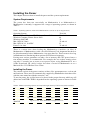
System Requirements
The parser has been run succesfully on Mathematica 4 to Mathematica 6.
Mathematica 6 currently is supported for a range of operating systems, as shown in
Table 1:
Table 1. Operating systems under which Mathematica 6 can be run (at 27 august 2007).
Operating System
Windows Vista, Windows XP, Windows Server 2003
Windows Compute Cluster Server 2003
Windows 2000, ME
Mac OSX 10.3 Intel
Mac OSX 10.3.9, 10.4 PPC
Linux 2.4 or later
32/64 bit
32 and 64
64
32
32 and 64
32
32 and 64
There is a minor issue when loading the Mathematica 6 modules (.m files) in
Mathematica 4: Mathematica 6 adds a few $CellContext`Code fragments that have to
be deleted manually before Mathematica 4 can open the files. There seems to be a bug
in Mathematica 6 introducing these spurious $CellContext fragments.
Parsing more serious grammars can take a lot of memory and CPU power, hence a
fast modern machine is recommended. For example, the row reduce strategy alone
can take 15 seconds just to create a new parser object, using Mathematica 4 on a
1GHz Powerbook G4, while it takes less than a second in Mathematica 6 on a
Macbook Pro 2.33 GHz Intel Core 2 Duo.
Installing the Parser
The current version of the parser consists of three files: parstratparser.m, code.m and
unification.m. These are files automatically compiled by Mathematica from three files
with the same name but with the extension ".nb".
To use the parser, the .m files have to be placed in the proper directory which we will
abbreviate with TDIR. TDIR is dependent on the operating system as shown in Table
2:
Table 2. Different operating systems and required target directory TDIR for the parser modules.
OS
Mac OSX
Linux
Windows 98/Me
Windows NT
Windows
2000/XP
TDIR
$HOME/Library/Mathematica/Applications
$HOME/.Mathematica/Applications
C:\Windows\Application Data\Mathematica\Applications
C:\WINNT\Profiles\username\
Application Data\Mathematica\Applications
C:\Documents and Settings\username\
Application Data\Mathematica\Applications
3
In general the directory is $UserBaseDirectory/Applications, and $UserBaseDirectory
is a Mathematica variable pointing to the system-dependent directory where
Mathematica expects the files.
Just drag all .m files into the TDIR directory, or use a shell command like
cd <directory where package was downloaded>
cp *.m $TDIR
If you want to use symbolic links instead of a copy: only symbolic links (made with
the -s option in ln) work properly. In OSX, it is possible to create another type of links
called 'alias' using option+apple+drag, but these links will not work for Mathematica.
4
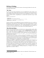
Writing a Strategy
The following sections describe the structure of the strategy definition, the rules, the
term and the start symbol.
The Term
In general, the term under manipulation can be any Mathematica object. Table 3 gives
a few sample terms. Sample terms supposedly are built using some formalization of a
domain that the student is working on, such as some computation, a puzzle or a linear
algebra problem. Such a formalization is essential but outside the scope of this
manual.
Table 3. A few sample terms
s[s[s[0]]]
times[plus[s[0],s[s[0]]],s[s[0]]]
LZMatrix[{1, 2, 3, 4}, {2, 3, 5, 7}, {3, 5, 7, 13}]
LZMatrix[{1,2},{RealVar["h"],LZTimes[2,5]}]
MUPuzzle[u,i,i,i,u,u,i]
Conflicts with the existing Mathematica function definitions have to be avoided, as
Mathematica would grab any object matching one of the existing functions, in order
to apply that function. For instance, the "Plus" symbol (with upper case P) is already a
'reserved' keyword in Mathematica, and a term Plus[Plus[0]] would instantly be
rewritten to 0, before the parser or the student would attempt anything on it.
The Attributed Name
Rewrite rules and grammar rules are referred to by a name, possibly together with a
number of attribute values. This reference is called an attributed name. An attributed
name is represented internally as a gterm structure. In Table 6 these names appear in
front of the ":" in each rule. Attributed names (gterms) occur very frequently in a
strategy specification, and therefore the text "gterm" is left out when prettyprinting to
make things more readable.
The name of the rewrite rule is a lower case string. The attributes are variables that
live inside the parser, and have the form $ followed by a lowercasestring, e.g. $row.
Attributes can be used more than once in an attributed name, as was illustrated by the
somerulename[$x,$x]. It is even possible to use general Mathematica-style constructs,
such as somename[gterm["2"],bla[$x,$y]] as an attributed name1.
Attributes are unified (e.g. [Baader01], p.454) with the 'function call'. For instance, if
somerulename[1,$y] is called using the definition of somerulename in Table 6, $x
would be set to 1, and if the rule can be applied, on return $y would also be set to 1.
As will be shown in subsequent sections, a rewrite rule can be applied on a term (see
the section The Term), by referring to the attributed name of the rule. Attributes can
be completely instantiated (e.g., RepExp[Strat25]]), may be left uninstantiated (e.g.,
aap[$pos] ) or instantiated partially (RepExp[aap[$pos]]). Example rewrite rule
applications are shown in Table 4.
1
This is unusual in attribute grammars, and not recommended. Also this feature was
not thoroughly tested.
5
Table 4. Few example rule applications with Table 6. On the right are the non-prettyprinted
versions of these rules
pretty printed
ruleexchrows[1,2]
Strat25
ruledeletevariable[$x]
RepExh[$s]
aap[beer[$x],$pos]
non pretty printed gterm
gterm["ruleexchrows",1,2]
gterm["Strat25"]
gterm["ruledeletevariable ",$x]
gterm["RepExh",$s]
gterm["aap",gterm["beer",$x],$pos]
Code Block
A Code block is a fragment of raw Mathematica code. Table 5 shows a few example
Code blocks.
Table 5. Some example Code blocks. The third example is showing the RuleAtPos embedding
the Code block, to make clear that the pattern variables "mat" and "vars" used in the Code
block get their values from the term at hand.
Code[If[$start > $end, $Failure, $var = $start]]
Code[Clear[$var]; $startp1 = $start + 1]
RuleAtPos[AugmentedMatrix[mat_LZMatrix,vars_],{},
Code[If[$k === 0 , $Failure,
$newmat = mat; $newmat[[$row]] = $k mat[[$row]];
AugmentedMatrix[$newmat, vars]]]
Only attribute variables should be used as a computational variable inside a code
block. Normal Mathematica variables (e.g. "k", as opposed to $k) should be avoided.
The reason is that any value given to normal Mathematica variables would be stored
in the global scope, and appear to all other evaluations at once. Proper scope
restriction to the rule at hand is provided only for the attribute variables.
If there is a problem evaluating the code contents by Mathematica, this will be caught.
An error message will be printed and the parser continues as if the Code returned
$Failure. For example, evaluating Code[3 = 4] (using CodeEval[{}, Code[3 = 4]])
gives
Set::setraw : Cannot assign to raw object 3. >>
Problem with strategy. Code block is incorrect. Intercepted
and returning $Failure instead. Code block: Code[3 = 4]
Code blocks have a number of important properties:
• A Code block has attribute HoldAll, so nothing inside a Code block is evaluated
until it is given to the CodeEval function.
• A Code block that returns $Failure causes all associated parser attempts to fail.
• Inside a Code block one can refer to $CurrentTerm, to determine the actual term at
that point.
• An attribute variable can be cleared using Mathematica's Clear[].
Although a Code block looks pretty straightforward, the technical implementation is
surprisingly tricky and may cause subtile problems. To overcome these, it may be
necessary to understand exactly what happens during evaluation of a code block.
First, all attribute variables occuring inside the Code block are collected, and shielded
from the general scope by using a Module call. Inside this shielded scope, the attribute
variables are set to their initial values. Then, Mathematica is asked to evaluate the
program inside the Code block. Control is passed directly to Mathematica, and
anything allowed by Mathematica can be done here. Next, the return value as well as
the new values of the attribute variables are collected. The Code block is analysed, to
6
determine which attribute variables occured on the left side of an equation or inside a
Clear. Only for these variables, the new values are saved, the other values are
discarded. While saving the values, it is checked for each variable if it actually still
has a value (it may have been Cleared), and if it was cleared the variable is removed
from the list of known variables instead of saved.
One known issue with this algorithm becomes clear in the following example with the
start condition $g=f[$x] and $k<0:
Code[If[$k<0,$x=6,$g=3]]
In this code block, $g might be changed (because $g is at the left of an assignment,
and we do no analysis of If-blocks), and therefore the value of $g is re-computed after
evaluation of this code block. In this case $x=6 after evaluation, and therefore $g=f[6]
after evaluation of this code block, even though $g was never modified in the code
block itself. In this case, a Clear[$x] in a subsequent Code block will NOT return
$g=f[$x] but leave us with $g=f[6].
The Rewrite Rules
This section discusses the rewrite rules in a top-down way. A rewrite rule contains
three parts:
1. The attributed name (the rule name and its attributes),
2. A mathematica pattern with a position, indicating when and where a rule can be
applied, and
3. The result, that specifies the new subterm replacing the current term at position pos.
In general, a rewrite rule looks as follows in pretty-printed format:
name(attributes): mathpattern @pos result
In un-pretty printed format, which is what has to be typed in by the strategy
programmer, this looks as follows:
RewriteRule[gterm["name",attributes...],
pos,result]
RuleAtPos[mathpattern,
In this manual we will usually use the pretty printed format, to keep things readable.
Informally, this rewrite rule stands for the following procedure: if someone wants to
apply a rewriterule, he gives the attributed name of that rule, but with some of the
attributes instantiated as needed.
First, a test is done if the pattern at the given position pos in the current problem term
matches the mathpattern. If the pattern matches, the matching subterm is replaced
with the (maybe computed) result. If the result is $Failure, the rewrite rule is
considered not to be applicable (even though the pattern matched the term).
The strategy specification contains a list of these rewrite rules. There should be at
most one rewrite rule matching the given attributed name, such that the result of the
rewrite is uniquely defined.
Before going in further detail, Table 6 shows a few example rules. The
ruledeletevariable shows that the result may even be empty.
7
Table 6. A few sample rules.
ruleplusx:= plus[s[x_],y_] @{} plus[x,s[y]]
ruleexchrows[$row1,$row2]:= mat_LZMatrix @$pos Code[$newmat = mat;
$newmat[[$row1]] = mat[[$row2]]; $newmat[[$row2]] = mat[[$row1]] ;$newmat]
rulescalerow[$row,$k]:= mat_LZMatrix @$pos Code[If[$k === 0 , $Failure,
$newmat = mat; $newmat[[$row]] = $k mat[[$row]]; $newmat];
ruledeletevariable[$pos]:= RealVar[x_] @$pos
somerulename[$x,$x]:= bla(1) @$pos $x
applyatpos[$pos]: bla(1) @$pos 1
To illustrate the use of a rewrite rule, we use the parser support function
ApplyRewriteRule that can apply a rule (the first argument) to a term (the third
argument) at a given position (2nd argument). For example, evaluating
ApplyRewriteRule[ RuleAtPos[aap[3], $pos, kat[3]],
{$pos == {3}},
beer[aap[4], aap[5], aap[3], aap[6], aap[3], aap[4]]]
gives
beer[aap[4], aap[5], kat[3], aap[6], aap[3], aap[4]]
More details are given in the following sections.
The Mathpattern and Position
The mathpattern is a standard Mathematica patterned object, see for instance
[Wolfram07a] or our previous report [Pasman07]. The pattern variables are set by
matching against the term at hand, and these variables are subsequently substituted in
the result.
Additional there is the pos information attached to it, indicating at which position in
the term the pattern should match. This position is using the conventional
Mathematica format to return positions as a list of child numbers, see for instance
[Wolfram07b].
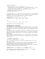
All used attributes, including the position, have to be set properly, so that the pattern
can be matched properly and the result can be computed if necessary. Figure 1
illustrates this
S:= Code[$m={}] myrule[$m]
myrule[$x]:= RuleAtPos[aap[3], $x, kat[3]]
Figure 1. Code snippet illustrating how the attribute $m is instantiated properly in the rule for S
before myrule is 'called'.
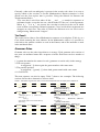
Note that the position only refers to the top level position. The mathpattern may still
contain ambiguities concerning the positions of subterms. Figure 2 uses
Mathematica's ReplaceList to show that Mathematica rewrite rules may be ambiguous
on more places than just the position of the top of the rule.
ReplaceList[aap[1, 2, 3, 4], aap[x__, y__] -> aap[X[x], Y[y]]]
{aap[X[1], Y[2, 3, 4]], aap[X[1, 2], Y[3, 4]], aap[X[1, 2, 3], Y[4]]}
Figure 2. ReplaceList example showing that the rewrite rule aap[x__, y__] -> aap[X[x],
Y[y]] can be applied in many – in this case, three – ways.
8
Currently, when such an ambiguity is present in the rewrite rule, there is no way to
specify which of the rewrites is needed. Mathematica's Replace function is used,
which uses the first replace that is possible. Citing the manual for Patterns and
Transformation Rules:
"The case that is tried first takes all the __ and ___ to stand for sequences of
minimum length, except the last one, which stands for "the rest" of the arguments.
When x_: v or x_. are present, the case that is tried first is the one in which
none of them correspond to omitted arguments. Cases in which later arguments are
dropped are tried next. The order in which the different cases are tried can be
changed using Shortest and Longest."
The Result
The result can be either a direct Mathematica construct as in ruleplusx (Table 6), or a
Code block returning the new subterm. In the Mathematica object, it is possible to
refer both to the pattern variables as used in the Pattern, and to the attributes as used
in the attributed name.
Grammar Rules
Grammar rules are the other ingredient to a strategy. Each grammar rule consists of
two parts: an attributed name and a sequence of terms. Each term can be a number of
things:
1. A gterm that matches the name of a rule (grammar or rewrite rule) in the strategy
2. The not operator:
A not[gterm[...]] where again the gterm matches with some name
3. The parallel operator:
A par[gterm[...], gterm[...]] where both gterms match with some name
4. A Code block
The term sequence can also be empty. Table 7 shows a few examples. The following
sections discuss these alternatives in more detail.
Table 7. Examples of grammar rules. The fourth example shows an empty term sequence.
pretty printed grammar rule
non-prettyprinted
GrammarRule[gterm["Strat25d1"],
{gterm["Strat25a"],
gterm["Strat25b"],
gterm["Strat25c"] }]
GrammarRule[
gterm["Strat25b2MaybeScale1",
$firstuncoveredrow, $j, $k],
{Code[
If[$k == 1 , $Failure, $factor
= 1/$k] ],
gterm["scalerow",
$firstuncoveredrow, $factor]}]
GrammarRule[gterm["RepExh", $s],
{$s, gterm["RepExh", $s]}]
GrammarRule[gterm["N", $s], {}]
GrammarRule[gterm["RepExh", $s],
{not[$s]}]
Strat25d1:=Strat25a Strat25b
Strat25c
MaybeScale1[$firstuncoveredrow, $j,
$k] :=
Code[If[$k == 1, $Failure,
$factor =
1/$k]]
scalerow[$firstuncoveredrow,
$factor]
RepExh[$s]:= $s RepExh[$s]
N[$s]:=
RepExh[$s]:=not[$s]
9
The parser can determine applicable positions for a pattern, but it does so only when
testing whether a strategy is applicable (e.g. when evaluating a "not(strategy)"
construct, see the section Not Operator).
The Meaning of a Grammar Rule
The presence of a grammar rule in a strategy means that the attributed name of the
rule can be applied if the sequence of terms associated with the rule can be applied in
the given order.
To give an example, assume we have the strategy
rewriterules:
setto0[$x,$pos]:= $x @pos 0
grammarrules:
S:=setto0[cat,{1}] setto0[bear,{2,1}]
S:=setto0[dog,{3}]
T:=setto0[cat,{2}]
then the first grammar rule for S can be applied succesful to the term
aap[cat,dog[bear,3]] because application of setto0[cat,{1}] on this term is
possible and results in the new term aap[0,dog[bear,3]]. setto0[bear,{2,1}]
can then be applied on the result, giving the final term aap[0,dog[0,3]]. The second
rule for S and the rule for T however can not be applied succesfully because they do
not have the right terms at the right place.
In the end, the grammar rules refer to rewrite rules. These rewrite rules are
transforming the term at hand; the grammar rules mainly serve to generate all good
sequences of rewrite rules.
Not all rewrite sequences defined by the strategy have to be applicable to the actual
term. But if it is applicable, the resulting term after rewriting should be a good
solution.
If multiple rules can be applied (for instance, with the start term aap[cat,0,dog]) ,
the grammar is ambiguous for the given term. In extreme cases the grammar could
even be ambiguous for any term.
A strategy is a set of rules, combined with a start name (with attributes). We say that
the strategy is applicable on the term if the start name can be applied to the term.
If a strategy is applicable, this means that application of one of the rewrite sequences
leads to a final result. That result then is supposed to be a "good" final answer to the
problem term.
Attributes are filled in as late as possible. For instance with a rule like
N[$x]:=$x [ $x = Substitute] $x [$x=Add] $x
A call to N[Mul] will effectively "unfold" into the strategy Mul Substitute Add.
Code Block
A Code block in a grammar rule has a slightly different meaning from a Code block in
a rewrite rule. If the Code block returns $Failure, the effect is the same as before: the
associated parse attempt fails. But all other return values are ignored. Here, the Code
block is used for its side effects: setting/clearing attribute values properly.
Not Operator
The not[X] operator checks that a attributed name X can not be applied. The not can
be "applied" if X can not be applied. In order to test this, the parser creates a
10
temporary parser for the current term at hand, and tries to apply X to it. If there is a
way to do that, the not fails and not[X] can not be applied. On the other hand, if there
is no way to apply X, the not[X] can be "applied". The temporary parser is then
thrown away, and the not[X] is thus applied without changing anything in the term at
hand.
The not operator is slightly special:whenever the parser is testing a not, rewrite rules
can be called without having the $pos variable being set. If it is not set, the parser will
try all potential positions where the rule can be applied. For each applicable position,
$pos will be set accordingly2 and further parsing is tried.
Parallel Operator
The par[X,Y] operator checks that attributed name X and Y can be applied in parallel,
interleaved. Either X or Y can "eat" the the next rewrite actions of the user.
The parser internally needs to keep track of all possible inbetween results of X and Y.
With excessive ambiguity, the parser may run out of memory. Therefore it is
important to minimize ambiguity of X and Y. This problem can also occur if one
parser makes multiple assignments to a variable. As with ambiguity, all these possible
assignments have to be tracked separately and excessive occurances may cause
excessive memory and CPU usage.
It is possible to share attributes between X and Y. Shared attributes are those
attributes that occur in both X and Y within the par[]. So in the call
par(T($x,5,aap($w),$z), U($z,ga($w),$c) ) the attributes $z and $w occur in both
heads and thus are shared between T and U. This way, the parsers for X and Y can
"communicate" about their progress and influence the other parser3.
Some restrictions apply on where two interleaved parsers X and Y can actually
interleave. This is currently hard-coded in the function CanInterruptHere, which
prevents switching the eating to the other parser when the eating parser is just before a
Code block.
2
This is not possible during normal parsing, as each different application position
requires a separate parser.
3
Due to a bug, it is currently necessary to use the exact name also in the called names.
So in given example, one should define T[...,$z] and refer to $z. T[...,$g] for instance
will not work properly, and $g would not work as a shared variable.
11
Using a Parser
Using the parser comprises four steps: creating an initial parse state, feeding student
rewrite steps to it, checking the status of the parse state and extracting a hint. Parsing
in this system means extending the parse state.
Initializing the Parser
In order to use the parser, the parser has to be initialized properly. This chapter
describes the parts that need to be set up: the strategy containing the rewrite rules, the
grammar rules and the start term, and the term under manipulation.
First, the parser has to be loaded. This can be done using
Needs["parstratparser`"];
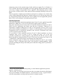
Next, the grammar and rewrite rules have to be defined. For example, we can enter a
set of rules and a grammar G3 as in Figure 3:
rulea = RewriteRule[gterm["a"],RuleAtPos[a,$somewhere,1]];
ruleb = RewriteRule[gterm["b"],RuleAtPos[b,$somewhere,1]];
G1 = {
GrammarRule[gterm["S"],{par[gterm["A",$x],gterm["B",$x]]}],
GrammarRule[gterm["A",$x],{gterm["a"],Code[$x=1]}],
GrammarRule[gterm["A",$x],{gterm["a"],Code[$x=2]}],
GrammarRule[gterm["B",$x],{gterm["b"],Code[If[$x=!=1,$Failure]]}]
};
Figure 3. Two rewrite rules and an example grammar doing parallel substitution of a and b in a
term.
Pretty printing is possible for all components of the parse state, making it easier to
assess the parse state and results. Any component of a parse state can be plugged into
the function PToString[object] , returning a prettyprinted string of the object.
PToString for Mathematica lists can be given an additional character to use for item
separator. For instance PToString[{1,2,3},"--"] will give "1--2--3".
The grammar can be pretty-printed using PToString, e.g. PToString[G1, "\n"],
giving
S:=(A[$x]//B[$x])
A[$x]:=a Code[$x = 1]
A[$x]:=a Code[$x = 2]
B[$x]:=b Code[If[$x =!= 1, $Failure]]
Then, a parser is set up with a call
ps = newparser[gramrules, rewrules,term,grammarstartsymbol]
where gramrules (a plain list of grammar rules) gives the grammar rules to be used,
rewrules (a plain list of rewrite rule items) is the set of rewrite rules to be used, term is
the start term, grammarstartsymbol is the start symbol (actually, an attributed name)
for the parser, and ps is an arbitrary Mathematica symbol used to store the resulting
initial parse state. The ps stands for "parse state", and is an intermediary parse result
whose properties, such as "parse finished" or "parse failed", can be checked as
described in the next chapter.
for our example, the call needs to be
12
ps=newparser[G1, {rulea, ruleb}, {a, b}, gterm["S"]];
The parser may output a lot of debug messages during parsing. You can turn these off
with Clear[DPPrint].
You can view the fresh parser using PToString, e.g. PToString[ps], giving
Head:S
<SET 1--term:{a, b}
items:<item$2401:S•(A[$x]//B[$x]) vars: pred:{} suc:{}>
pitem[1, subp$2469]
shiftpos:
SUBPARSER subp$2469 for (A[$x]//B[$x]){
***Pair with eatpattern ''. status:ontrack
Parser 1
Head:A[$x]
<SET 1--term:{a, b}
items:<item$2419:A[$x] •a Code[$x = 1] vars: pred:{} suc:{}>
<item$2431:A[$x] •a Code[$x = 2] vars: pred:{} suc:{}>
shiftpos:
>
Parser 2
Head:B[$x]
<SET 1--term:{a, b}
items:<item$2457:B[$x] •b Code[If[$x =!= 1, $Failure]] vars: pred:{}
suc:{}>
shiftpos:
>
***}
END SUBPARSER subp$2469
>
Explanation of these parser contents is out of the scope of this user manual, see the
technical reference manual for details [Pasman07b].
Nothing has been "parsed" at this point: what has to be parsed are actions made by the
student and these actions are not yet given. The subparser however tested that there
exists at least one way to complete the parse of A//B, as witnessed by the
"status:ontrack" tag in the subparser.
Feeding Student Actions
Parsing can be continued from any parse state, using Scanner[old state,
gterm[rewrite...], newterm] where
• old state is the parse state that is to be continued,
• gterm[terminal...] is the next action that the student took (which therefore must be
a rewrite step with its associated attributes) and
• new term is the result term after application of the rewrite step4.
Scanner returns the resulting new state. The old state is unaffected. To continue the
example, reflecting the student doing rewrite action a, enter
ps1 = Scanner[ps, gterm["a"], {1, b}];
4
If the rewrite rule is available, the new term could be computed. But in some cases
the rule may be known to the student support system but unknown to the parser.
13
and to reflect the student's next action "b" enter
ps2 = Scanner[ps1, gterm["b"], {1, 1}];
As described in the next sections, you can apply several functions on the resulting
parse states, to check the status, create parse graphs, etc.
Checking the Parse State
The easiest way to check the status of a parse is using Status[parsestate]. It returns
finished, ontrack or dead. finished means that the start symbol has currently been
recognised, so the start symbol ate exactly all student actions. ontrack means that the
parse is not yet finished but that it can be finished by adding appropriate actions. And
dead means that this parse is not finished and it can not be finished either.
So we can ask Status[ps1] or Status[ps2], giving ontrack and finished.
Testing for ontrack, which is part of the Status function, may be expensive. This is
because the parser will actually try to finish the parse by inventing new subsequent
actions and try how they work out. Checking for Finished only using the
Finished[state] function is much cheaper because it does not do this ontrack test.
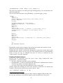
Creating a Hint
Internally, creating a hint is usually a two-step process. First, a given parse state is
extended using TryToComplete, which returns a new "finished" parse state by adding
actions to the given state if possible. If not possible, this returns $Failure. For
example,
suggestion = TryToComplete[ps1];
Finished[suggestion]
where Finished returns True.
Strictly, this new parse state contains all information about how to reach the finished
state from the given state. However, extracting this information is a complex task
because all possibile ambiguities are still in this parse state, as well as all failed parse
attempts. To create a hint, only one parse tree representing a good solution would be
more useful. The function ParseTreeForShift can extract a single unambiguous parse
tree from a parse state. The call is
tree = ParseTreeForShift[suggestion, FinishedShifts[suggestion][[1]]]
which returns in our example
node[gterm[ "S"], {parshift[par[gterm["A", $x], gterm["B", $x]], "01",
node[gterm["A", 1], {node[gterm["a"], {}]}],
node[gterm["B", 1], {node[gterm["b"], {}]}]]}]
There is a lot of debug output from this conversion, which can be turned off using
Clear[DHPrint].
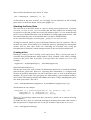
To make life easy, there is a function GetSuggestionTree[parsestate] that creates a
hint and generates a simple parse tree in one go. It returns a parse tree or $Failure:
tree = GetSuggestionTree[ps]
14
giving the same result as above. The parse tree is a very simple tree structure. It
contains objects node[nodeinfo,children], where nodeinfo is the relevant, instantiated
term from the rule sequence and children is an ordered list of children of that node.
With this tree, it should be easy to generate a proper hint, for instance by checking the
leaf nodes and checking where the student stands now, or by checking nodes higher
up in the tree and generate a higher-level hint. Currently, only extraction of the leaf
nodes is implemented, via GetTerminalsFromTree:
GetTerminalsFromTree[tree]
gives
{gterm["a"], gterm["b"]}
GetTerminalsFromTree accounts for the correct eat pattern as specified in parallel
nodes.
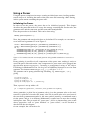
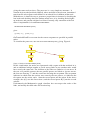
To visualize the parse tree, one can use VisualizeTree[tree], giving Figure 4.
S $13
(A[$x]//B[$x]) $14
//
01
A[1] $15
B[1] $17
a $16
b $18
Figure 4. Result of VisualizeTree[tree]
In this visualization, the nodes are represented with a square with the nodeinfo in it,
and an additional unique number to avoid wrong links in case another node would
have exactly the same info. The children of the nodes are linked to via an arrow. In
the case of a parallel operator, the two parallel parsers are linked to via two arrows,
the first one showing "//" and the second one showing the eat pattern. The eat pattern
indicates in which order the actions were eaten by the two parsers: a 0 indicates the
first parser ate the action, and a 1 that the second parser ate the action. In the above
example, the A[1] eats the first action a, and the second parser B[1] eats the second
action b.
Unfortunately the Mathematica graph visualizer does not respect the order of the
links, and usually the child order will be mixed up.
15
References
[Baader01]
Baader, F., & Snyder, W. (2001). Unification Theory. In J.A.
Robinson and A. Voronkov (Eds.), Handbook of Automated
Reasoning, 447–533. Elsevier Science Publishers
[Pasman91]
Pasman, W. (1991). Incremental Parsing. Master's thesis, University
of Amsterdam, Department of Computer Science, Amsterdam, the
Netherlands. Available Internet:
http://graphics.tudelft.nl/~wouter/publications/publ.html.
[Pasman07]
Pasman, W. (2007). Terms and Rules in the LA system. Technical
Report, Delft University of Technology, March.
[Pasman07b]
Strategy Parser Technical Reference Manual. Technical Report, Delft
University of Technology, August.
[Wolfram07a] http://reference.wolfram.com/mathematica/ref/Pattern.html.
[Wolfram07b] http://reference.wolfram.com/ mathematica/ref/Position.html.
16